Design of control network and survey for CSNS 、 Project Overview 2 、 Design of the Primary Control Network 3 、 Survey Scheme for the Surface Control Network 4 、 Design of the

Design of control network and survey for CSNS

Accelerator center of IHEPWang tong, Li bo

2012.09.11

1、Project Overview

2、Design of the Primary Control Network

3、Survey Scheme for the Surface Control Network

4、 Design of the Secondary Network

5、 Survey Scheme for the Tunnel Control Network

6、Alignment Scheme for Accelerator Components in Tunnel

Contents

1、Project Overview

China Spallation Neutron Source(CSNS) mainly consists of an H- linac and a proton rapid cycling synchrotron. It is designed to accelerate proton beam pulses to 1.6 GeV kinetic energy at 25 Hz repetition rate, striking a solid metal target to produce spallation neutrons.

1.1 Brief introduction

As shown in Table 1, the accelerator is designed to deliver a beam power of 100 kW with the upgrade capability to 500 kW by raising the linac output energy and increasing the beam intensity.

1.1 Brief introduction Table 1 CSNS primary parameters in

baseline Project phase I

Beam ave. power, kW 100Proton energy, GeV 1.6Ave. current, I, µA 62.5Repetition rate, Hz 25

Proton per pulse, 1013 1.63Pulse length, ns <500

Linac energy, MeV 80Linac peak current, mA 15

Target material TungstenNo. Moderators 3

No. neutron instruments 3

LinacRCS

Spectrometer

The length of the H- linac is about 197m, the circumference of the proton rapid cycling synchrotron(RCS) is about 228m, the length of the linac to RCS beam transport (LRBT) is about 40m, and length of the RCS to target transport(RTBT) is about 144m.

1.2 General layout of CSNS

CSNS locates in Guangdong province, which is in the south of China . The construction of CSNS is in progress.

2、Design of the primary network

2.1 Overall layout of primary networkThe control network of CSNS is classified into two

grades: the primary network and the secondary network.The primary network consists of 27 points, which is

distributed over the whole area of CSNS. It is used for the layout of buildings and facility and to provide high accuracy control for the secondary network .

The yellow points : permanent monuments based on bed rock in the tunnel.

The blue points : densification monuments built on the surface of ground.

2.2 Characteristic of primary networkThe permanent points in tunnel also belongs to the

secondary control network, they can’t directly connect with the other points on the ground. To carry out the survey, we should project them from tunnel to the roofs vertically. Wild NL nadir telescope will be considered for centering and projection.

the point is projected to the roof.

the permanent point in tunnel.

Perspective View

3、Survey scheme for the surface control network

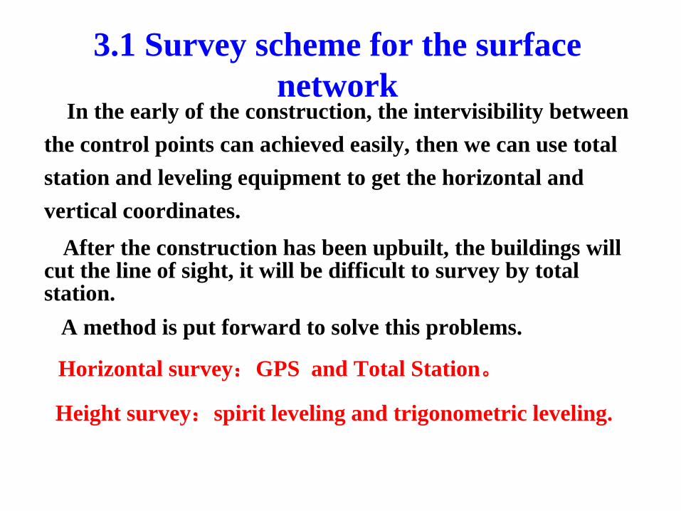
3.1 Survey scheme for the surface network

In the early of the construction, the intervisibility between the control points can achieved easily, then we can use total station and leveling equipment to get the horizontal and vertical coordinates.

After the construction has been upbuilt, the buildings will cut the line of sight, it will be difficult to survey by total station.

A method is put forward to solve this problems.

Horizontal survey：GPS and Total Station。

Height survey：spirit leveling and trigonometric leveling.

4 GPS receivers will be applied to measure the horizontal positions.

In each station, the GPS receivers are centered on every 4 monuments. With post-processing analysis ,we can finally get the length of baselines between these primary control points.

3.2 The method of horizontal survey

principle of GPS survey

baseline

G11HP11G12HP12

G13HP13G09HP09

G10HP10

P01 P02

P03P04

P05

P14

G15H

G16H

P06

P07

P08

Plan view of GPS survey

G11HP11

G12HP12

G13HP13

G09HP09

G10HP10

P01P02

P03P04

P05P14

G15H

G16H

P06P07

P08

Perspective view of GPS survey

G11HP11

G12HP12

G13HP13

G09HP09

G10HP10

P01P02

P03P04

P05P14

G15H

G16H

P06P07

P08

Side view of GPS survey

We can see that the lines of sight between points are cut off severely by the buildings. That’s the reason why we apply GPS to carry out the horizontal survey.

Owing to its many advantages, trigonometric leveling has been more and more applied in many fields.

The basic concept of trigonometric leveling can be seen from fig1. When measuring the vertical angle and the slant distance S is used, then the precision elevation difference between A and B is therefore:

3.3 The method of trigonometric leveling

( ) ( )( )

( )

2

2

2

tan

1 / 2

/ 2

/ 2

ABh D i v ff p r k D R

p D R

r k D R

α= • + − +

= + = −

=

= − •

“R” - the average radius of earth.“f” - effect of earth curvature and refraction.“p” - correction of earth's curvature.“r” – correction of atmospheric refraction.

total station

prism

To eliminate the uncertainty in the curvature and refraction correction, vertical-angle observations are measured at two ends of the lines as close in point of time as possible.

The correct difference in elevation between the two ends of the line is the mean of the two values computed by reciprocal observation. The formula are as follows:

3.3 The method of trigonometric leveling

total station

prism

G11HP11G12HP12

G13HP13G09HP09

G10HP10

P01 P02

P03P04

P05

P14

G15H

G16H

P06P07

P08G14L

G18H

G01H

Side view of trigonometric leveling

G11HP11G12HP12

G13HP13G09HP09

G10HP10

P01 P02

P03P04

P05

P14

G15H

G16H

P06P07

P08G14L

G18H

G01H

Side view of trigonometric leveling

To improve efficiency and reduce the working strength, a automatic measurement program based on Leica TDA5005 total station is developed in Visual C++ 6.0 visualization development environment.

By sending ASCII orders through the serial communication between computer and the instrument, it finally realize to control the total station as we want.

With this program, it can easily for us to measure with total station.

3.4 Automatic observation system based on Leica TDA5005

Interface of the programProgram debugging

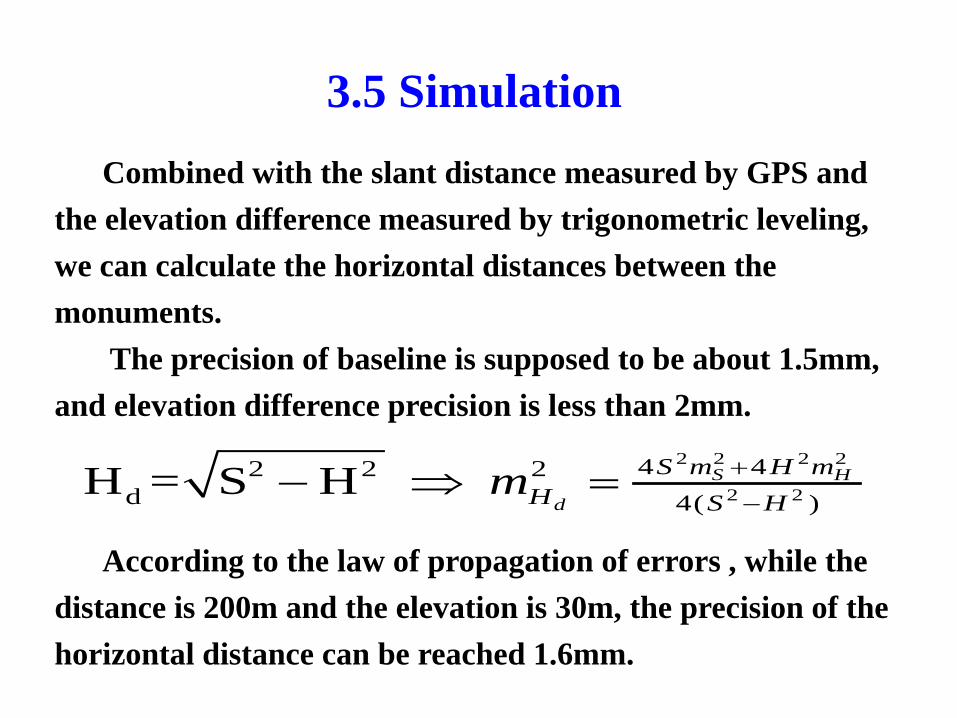
Combined with the slant distance measured by GPS and the elevation difference measured by trigonometric leveling, we can calculate the horizontal distances between the monuments.

The precision of baseline is supposed to be about 1.5mm, and elevation difference precision is less than 2mm.

3.5 Simulation

2 2 2 2

2 24 42 2 2

d 4( )H = S H S H

d

S m H mH S H

m +

−− ⇒ =

According to the law of propagation of errors , while the distance is 200m and the elevation is 30m, the precision of the horizontal distance can be reached 1.6mm.

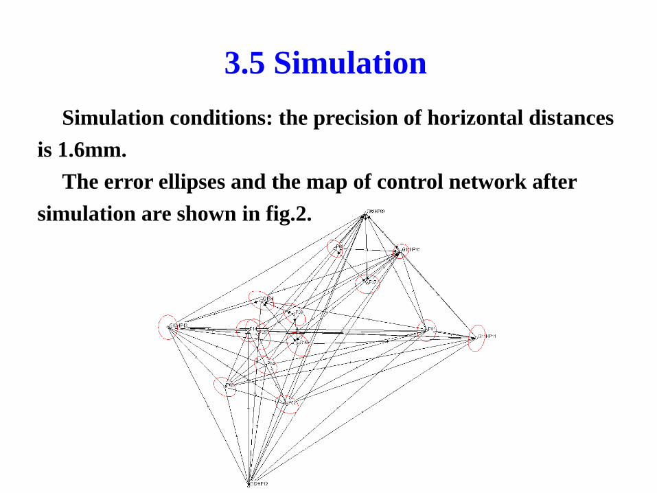
Simulation conditions: the precision of horizontal distances is 1.6mm.

The error ellipses and the map of control network after simulation are shown in fig.2.

3.5 Simulation

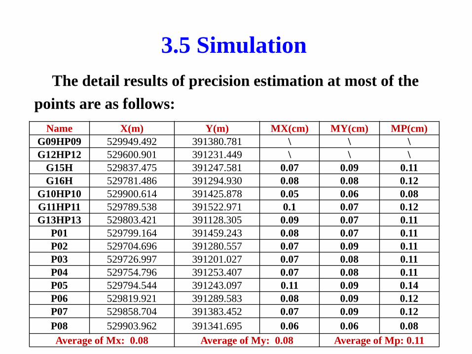
Name X(m) Y(m) MX(cm) MY(cm) MP(cm)G09HP09 529949.492 391380.781 \ \ \G12HP12 529600.901 391231.449 \ \ \

G15H 529837.475 391247.581 0.07 0.09 0.11G16H 529781.486 391294.930 0.08 0.08 0.12

G10HP10 529900.614 391425.878 0.05 0.06 0.08G11HP11 529789.538 391522.971 0.1 0.07 0.12G13HP13 529803.421 391128.305 0.09 0.07 0.11

P01 529799.164 391459.243 0.08 0.07 0.11P02 529704.696 391280.557 0.07 0.09 0.11P03 529726.997 391201.027 0.07 0.08 0.11P04 529754.796 391253.407 0.07 0.08 0.11P05 529794.544 391243.097 0.11 0.09 0.14P06 529819.921 391289.583 0.08 0.09 0.12P07 529858.704 391383.452 0.07 0.09 0.12P08 529903.962 391341.695 0.06 0.06 0.08Average of Mx: 0.08 Average of My: 0.08 Average of Mp: 0.11

3.5 SimulationThe detail results of precision estimation at most of the

points are as follows:

4、Design of the secondary network

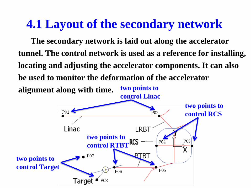
4.1 Layout of the secondary networkThe secondary network is laid out along the accelerator

tunnel. The control network is used as a reference for installing, locating and adjusting the accelerator components. It can also be used to monitor the deformation of the accelerator alignment along with time. two points to

control Linactwo points to control RCS

two points to control Target

two points to control RTBT

4.1 Layout of the secondary networkConsidering the capability of laser tracker and the precision

requirement of survey network, we plan to set control point sections with the interval of 6 m along the tunnel. In each section, there are five monuments, two on the floor, one on the inner wall, one on the outer wall and one on the roof.

There are 36 control point sections along the Linac tunnel, 7 sections in the LRBT tunnel, 44 sections along the RCS tunnel and 26 sections in the RTBT tunnel.

laser tracker

the wall monument in BEPCII

4.2 Constitution of the secondary network

According to the major structure of the accelerator complex, the network can be divided into the Linac-LRBT network, the RCS network, the RTBT network, the Target and Spectrometer network.

According to the ways of measurement and the methods of data processing, secondary control network can be divided into horizontal network and vertical network.

The secondary control network

Location

Linac-LRBT control network

RCS control network

RTBT control network

Target and Spectrometer control network

Application

Horizontal control network

Vertical control network

5、Survey scheme for the tunnel control network

5.1 Survey scheme for the tunnel networkLaser tracker is used to carry out the horizontal network survey and

vertical network survey together by free station method. The survey station is set between every two neighboring sections. At

each station, the laser tracker measures 3 backward sections and 3 forward sections. There are 5 control points in each section, so the laser tracker should measure 30 points at one station. The number of common control points between neighboring stations is 25. In order to obtain the horizontal coordinates and vertical coordinates, at each station we need to establish a horizontal datum for the laser tracker.

5.2 Enhanced survey for the tunnel network In order to improve the precision of Linac horizontal control network, we use a total station to carry out a enhanced hexagon network survey which covers the whole Linac.

As the vertical network surveyed by laser tracker is not closed, the yellow leveling line is added by Leica DNA03, which can effectively decrease the accumulated errors in the tunnel vertical network survey carried out by laser tracker.

5.3 Data process of the tunnel network

Horizontal adjustment schemeTake all the observations of every station as the input parameters,

including distances and angles measured by laser tracker and total stations, we can get the horizontal coordinates of the tunnel horizontal network.

Vertical adjustment schemeFrom the vertical coordinates measured by laser tracker and the height

differences of the monuments in the yellow line we can get a group of height differences of a closed leveling.

Using these height differences to do level adjust we can get the vertical coordinates of the tunnel level network.

5.4 Simulation

Horizontal Simulation

The Linac simulation results

The transverse point error:0.12mm (RMS)

The longitudinal point error:0.04mm (RMS)

The RCSsimulation results



The RTBTSimulation results



MSE of Laser Tracker:0.08mm 5″

MSE of Total Station:0.50mm 3″

Vertical SimulationMSE of Laser Tracker:0.074mm

MSE of Leveling:0.05mmThe height Simulation:0.058mm

The following diagram lists the simulation results of the tunnel control network :

6、Alignment scheme for accelerator components in tunnel

6.1 Tolerance requirement of major components

The alignment tolerance requirement of the major components in CSNS:

ΔX (mm)

Transverse offset

ΔY (mm)

Vertical offset

ΔZ (mm)

Longitudinal offset

Components in the RCS

0.20 0.20 0.30

DTL in the Linac

0.10 0.10 0.10

Components in the Linac

0.25 0.25 0.50

Components in the RTBT

0.25 0.25 0.50

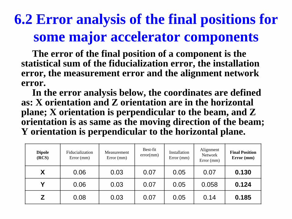
6.2 Error analysis of the final positions for some major accelerator componentsThe error of the final position of a component is the

statistical sum of the fiducialization error, the installation error, the measurement error and the alignment network error.

In the error analysis below, the coordinates are defined as: X orientation and Z orientation are in the horizontal plane; X orientation is perpendicular to the beam, and Z orientation is as same as the moving direction of the beam; Y orientation is perpendicular to the horizontal plane.

Dipole(RCS)

FiducializationError (mm)

Measurement Error (mm)

Best-fiterror(mm) Installation

Error (mm)

Alignment Network

Error (mm)

Final Position Error (mm)

X 0.06 0.03 0.07 0.05 0.07 0.130

Y 0.06 0.03 0.07 0.05 0.058 0.124

Z 0.08 0.03 0.07 0.05 0.14 0.185

Quadrupole

(RCS)

Fiducialization Error (mm)



Error (mm)

Alignment Network

Error (mm)


X 0.05 0.03 0.07 0.05 0.07 0.125

Y 0.05 0.03 0.07 0.05 0.058 0.119

Z 0.08 0.03 0.07 0.05 0.14 0.185

DTL

(Linac)




Error (mm)

Alignment Network

Error (mm)


X 0.04 0.03 0.06 0.04 0.12 0.149

Y 0.04 0.03 0.06 0.04 0.058 0.105

Z 0.04 0.03 0.06 0.04 0.04 0.096

6.2 Error analysis of the final positions for some major accelerator components

RFQ

(Linac)




Error (mm)

Alignment Network

Error (mm)


X 0.04 0.03 0.06 0.04 0.12 0.149

Y 0.04 0.03 0.06 0.04 0.058 0.105

Z 0.04 0.03 0.06 0.04 0.04 0.096

Quadrupole

(RTBT)




Error (mm)

Alignment Network

Error (mm)


X 0.05 0.05 0.07 0.05 0.16 0.195

Y 0.05 0.05 0.07 0.05 0.058 0.126

Z 0.08 0.05 0.07 0.05 0.10 0.162

6.2 Error analysis of the final positions for some major accelerator components

The end, thanks!

Documents

Design of control network and survey for CSNS 、 Project Overview 2 、 Design of the Primary Control Network 3 、 Survey Scheme for the Surface Control Network 4 、 Design of the