DESIGN OF AN OUTER-ROTOR BRUSHLESS DC MOTOR FOR CONTROLMOMENT GYROSCOPE APPLICATIONS

A THESIS SUBMITTED TOTHE GRADUATE SCHOOL OF NATURAL AND APPLIED SCIENCES

OFMIDDLE EAST TECHNICAL UNIVERSITY

BY

NECATI ÇAGAN

IN PARTIAL FULFILLMENT OF THE REQUIREMENTSFOR

THE DEGREE OF MASTER OF SCIENCEIN

ELECTRICAL AND ELECTRONICS ENGINEERING

FEBRUARY 2015

Approval of the thesis:

DESIGN OF AN OUTER-ROTOR BRUSHLESS DC MOTOR FOR CONTROLMOMENT GYROSCOPE APPLICATIONS

submitted by NECATI ÇAGAN in partial fulfillment of the requirements for the de-gree of Master of Science in Electrical and Electronics Engineering Department,Middle East Technical University by,

Prof. Dr. M. Gülbin Dural ÜnverDean, Graduate School of Natural and Applied Sciences

Prof. Dr. Gönül Turhan SayanHead of Department, Electrical and Electronics Engineering

Prof. Dr. H. Bülent ErtanSupervisor, Electrical and Electronics Eng. Dept., METU

Examining Committee Members:

Prof. Dr. Muammer ErmisElectrical and Electronics Eng. Dept., METU

Prof. Dr. H. Bülent ErtanElectrical and Electronics Eng. Dept., METU

Prof. Dr. M. Kemal LeblebiciogluElectrical and Electronics Eng. Dept., METU

Assoc. Prof. Dr. U. Murat LelogluGeodetic and Geographic Information Tech. Dept., METU

Dr. Burcu DönmezGuidance and Control Design Dept., ROKETSAN A.S.

Date:

I hereby declare that all information in this document has been obtained andpresented in accordance with academic rules and ethical conduct. I also declarethat, as required by these rules and conduct, I have fully cited and referenced allmaterial and results that are not original to this work.

Name, Last Name: NECATI ÇAGAN

Signature :

iv

ABSTRACT

DESIGN OF AN OUTER-ROTOR BRUSHLESS DC MOTOR FOR CONTROLMOMENT GYROSCOPE APPLICATIONS

Çagan, Necati

M.S., Department of Electrical and Electronics Engineering

Supervisor : Prof. Dr. H. Bülent Ertan

February 2015, 109 pages

Attitude control plays an important role in low-earth orbit (LEO) satellites. Agilityof such systems are quite crucial and degree of agility can be determined by the helpof the maneuver capability of actuators. Typical actuating systems in a low-earthorbit satellite are Control Moment Gyroscopes (CMG), and the electric motor typeused in such systems is the brushless DC motor. In this study, an outer-rotor designof permanent magnet brushless DC motor to be used in a satellite application isinvestigated and, the main characteristics and performance parameters such as torqueper unit weight, torque per unit volume, inertia contribution and power efficiency arediscussed. This design is compared with various designs in a finite-element analysisenvironment. In conclusion, the overall performance of the motor is handled anddistinct design advantages are stated.

Keywords: Control Moment Gyroscope, outer-rotor permanent magnet brushless DCmotor design, performance comparison

v

ÖZ

KONTROL MOMENT JIROSKOP UYGULAMALARI IÇIN ROTORU DISARIDAFIRÇASIZ DA MOTORU TASARIMI

Çagan, Necati

Yüksek Lisans, Elektrik ve Elektronik Mühendisligi Bölümü

Tez Yöneticisi : Prof. Dr. H. Bülent Ertan

Subat 2015 , 109 sayfa

Konum kontrolü, Alçak Dünya Yörüngesi uydularında önemli rol oynamaktadır. Butip sistemlerin atikligi kritiktir ve atiklik derecesi eyleyicilerin manevra yetenegi ilebelirlenir. Alçak Dünya Yörüngesi uydularındaki tipik eyleyici sistemler KontrolMoment Jiroskoplarıdır ve bu tip sistemlerde kullanılan elektrik motoru tipi FırçasızDogru Akım (DA) Motorudur. Bu çalısmada uydu uygulamasında kullanılmak üzererotoru dısarıda yer alan bir dogal mıknatıslı fırçasız DA motoru tasarımı incelenmekteve ana karakteristikler ile birim agırlık basına tork, birim hacim basına tork, eylemsizlikmomenti katkısı ve güç verimi gibi performans parametreleri tartısılmaktadır. Butasarım çesitli tasarımlarla sonlu elemanlar analizi ortamında kıyaslanmaktadır. Sonuçolarak, motorun toplu performansı ele alınmakta ve farklı tasarım avantajları ifadeedilmektedir.

Anahtar Kelimeler: Kontrol Moment Jiroskop, rotoru dısarıda dogal mıknatıslı fırçasızDA motoru tasarımı, performans karsılastırması

vi

To my family, my friends and all anxious souls...

vii

ACKNOWLEDGMENTS

I would like to express my sincere thanks to my thesis advisor Prof. H. Bülent ERTANfor his guidance, almost-infinite patience and endless support throughout the study.

I would also like to thank the examining committee members Prof. Muammer ERMIS,Prof. M. Kemal LEBLEBICIOGLU and Assoc. Prof. U. Murat LELOGLU forevaluating this study.

I would like to express my deepest thanks to Burcu DÖNMEZ, as well as my colleaguesand other chiefs in ROKETSAN.

I would like to give credits to Bagıs Altınöz and Reza Zeinali, for their help andwizardry on MATLAB and MAXWELL, respectively.

Additionally, thanks to everyone those somehow take part and provide necessaryencouragement during the whole study.

My final and the most important thanks go to my parents, M. Tugrul ÇAGAN andÖznur ÇAGAN, undoubtedly, for their worthy and unrequited love, support and trust.

viii

TABLE OF CONTENTS

ABSTRACT . . . . . . . . . . . . . . . . . . . . . . . . . . . . . . . . . . . . v

ÖZ . . . . . . . . . . . . . . . . . . . . . . . . . . . . . . . . . . . . . . . . . vi

ACKNOWLEDGMENTS . . . . . . . . . . . . . . . . . . . . . . . . . . . . . viii

TABLE OF CONTENTS . . . . . . . . . . . . . . . . . . . . . . . . . . . . . ix

LIST OF TABLES . . . . . . . . . . . . . . . . . . . . . . . . . . . . . . . . xiv

LIST OF FIGURES . . . . . . . . . . . . . . . . . . . . . . . . . . . . . . . . xvi

LIST OF ABBREVIATIONS . . . . . . . . . . . . . . . . . . . . . . . . . . . xx

CHAPTERS

1 INTRODUCTION . . . . . . . . . . . . . . . . . . . . . . . . . . . 1

1.1 Scope of Thesis . . . . . . . . . . . . . . . . . . . . . . . . 1

1.2 Outline of Thesis . . . . . . . . . . . . . . . . . . . . . . . . 1

2 ACTUATING SYSTEMS IN LEO SATELLITES AND TYPICALELECTRICAL MOTORS . . . . . . . . . . . . . . . . . . . . . . . 3

2.1 General Overview . . . . . . . . . . . . . . . . . . . . . . . 3

2.2 Motor Selection for CMG Applications . . . . . . . . . . . . 5

2.3 General Overview of Brushless DC Motors . . . . . . . . . . 8

2.3.1 Control of Brushless DC Motors . . . . . . . . . . 10

ix

3 PROBLEM DEFINITION AND MOTOR ARCHITECTURE SELEC-TION . . . . . . . . . . . . . . . . . . . . . . . . . . . . . . . . . . 13

3.1 Problem Definition and The Requirements . . . . . . . . . . 13

3.1.1 Problem Definition . . . . . . . . . . . . . . . . . 13

3.1.2 Requirements . . . . . . . . . . . . . . . . . . . . 15

3.1.2.1 Functional Requirements . . . . . . . 15

3.1.2.2 Motor Torque Characteristics . . . . . 15

3.1.2.3 Cooling and Temperature Characteristics 17

3.2 Material Selection . . . . . . . . . . . . . . . . . . . . . . . 20

3.2.1 Ferromagnetic Materials . . . . . . . . . . . . . . 20

3.2.2 Permanent Magnets (PM) . . . . . . . . . . . . . . 22

3.2.2.1 Permanent Magnet Selection Criteria . 24

3.3 Magnetic Circuit . . . . . . . . . . . . . . . . . . . . . . . . 26

3.4 Back emf and Torque Equations for PM Brushless DC Motors 29

3.4.1 Back EMF and Torque . . . . . . . . . . . . . . . 30

3.4.2 Radial Flux Motor Equations . . . . . . . . . . . . 30

3.4.2.1 Back emf and Torque Equations underSinusoidal Excitation . . . . . . . . . 30

3.4.2.2 Back emf and Torque Equations underSquarewave Excitation . . . . . . . . 31

3.4.3 Axial Flux Motor Equations . . . . . . . . . . . . 32

3.4.3.1 Back emf and Torque Equations underSinusoidal Excitation . . . . . . . . . 32

x

3.4.3.2 Back emf and Torque Equations underSquarewave Excitation . . . . . . . . 33

3.5 Literature Survey . . . . . . . . . . . . . . . . . . . . . . . 34

4 DESIGN PROCEDURE OF OUTER-ROTOR BRUSHLESS DC MO-TOR TOPOLOGIES . . . . . . . . . . . . . . . . . . . . . . . . . . 37

4.1 Introduction to the Design of an Outer-Rotor Permanent Mag-net Brushless DC Motor Configuration . . . . . . . . . . . . 37

4.1.1 Preliminary Design Considerations . . . . . . . . . 38

4.2 Design Procedure of RF Motors under Sinusoidal Excitation . 38

4.2.1 Magnetic Circuit of RF Motors . . . . . . . . . . . 39

4.2.2 Determination of Motor Dimensions for SinusoidalExcitation . . . . . . . . . . . . . . . . . . . . . . 42

4.2.3 Winding Design . . . . . . . . . . . . . . . . . . . 46

4.2.4 Equivalent Circuit Parameters . . . . . . . . . . . 47

4.2.4.1 Phase Resistance . . . . . . . . . . . 47

4.2.4.2 Phase Inductance . . . . . . . . . . . 48

4.2.5 Losses . . . . . . . . . . . . . . . . . . . . . . . . 50

4.2.6 Motor Mass, Volume, Inertia and Efficiency . . . . 51

4.3 Design Procedure of RF Motors under Squarewave Excitation 53

4.3.1 Determination of Motor Dimensions for Square-wave Excitation . . . . . . . . . . . . . . . . . . . 53

4.3.2 Winding Design . . . . . . . . . . . . . . . . . . . 55

4.3.3 Equivalent Circuit Parameters . . . . . . . . . . . 55

4.3.4 Losses . . . . . . . . . . . . . . . . . . . . . . . . 56

xi

4.3.5 Motor Mass, Volume, Inertia and Efficiency . . . . 56

4.4 Design Outputs . . . . . . . . . . . . . . . . . . . . . . . . 57

4.4.1 Comparisons between Pole Numbers . . . . . . . . 57

4.4.2 Comparisons between Excitations . . . . . . . . . 58

5 ANALYTICAL RESULTS . . . . . . . . . . . . . . . . . . . . . . . 63

5.1 Analytical Results . . . . . . . . . . . . . . . . . . . . . . . 63

5.1.1 Analytical Results of Sinusoidal Designs . . . . . 65

5.1.1.1 Sinusoidal 2-pole Design . . . . . . . 65

5.1.1.2 Sinusoidal 6-pole Design . . . . . . . 66

5.1.2 Sizes and Performance Evaluation of SquarewaveDesigns . . . . . . . . . . . . . . . . . . . . . . . 67

5.1.2.1 Squarewave 2-pole Design . . . . . . 67

5.1.2.2 Squarewave 6-pole Design . . . . . . 68

5.2 Overall Performance Comparison . . . . . . . . . . . . . . . 68

6 SIMULATION RESULTS . . . . . . . . . . . . . . . . . . . . . . . 71

6.1 Simulation Results . . . . . . . . . . . . . . . . . . . . . . . 71

6.1.1 Simulation Results of Sinusoidal Designs . . . . . 72

6.1.1.1 Sinusoidal 2-pole Design . . . . . . . 73

6.1.1.2 Sinusoidal 6-pole Design . . . . . . . 76

6.1.2 Simulation Results of Squarewave Designs . . . . 79

6.1.2.1 Squarewave 2-pole Design . . . . . . 80

6.1.2.2 Squarewave 6-pole Design . . . . . . 82

xii

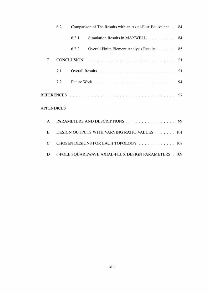
6.2 Comparison of The Results with an Axial-Flux Equivalent . . 84

6.2.1 Simulation Results in MAXWELL . . . . . . . . . 84

6.2.2 Overall Finite Element Analysis Results . . . . . . 85

7 CONCLUSION . . . . . . . . . . . . . . . . . . . . . . . . . . . . . 91

7.1 Overall Results . . . . . . . . . . . . . . . . . . . . . . . . . 91

7.2 Future Work . . . . . . . . . . . . . . . . . . . . . . . . . . 94

REFERENCES . . . . . . . . . . . . . . . . . . . . . . . . . . . . . . . . . . 97

APPENDICES

A PARAMETERS AND DESCRIPTIONS . . . . . . . . . . . . . . . . 99

B DESIGN OUTPUTS WITH VARYING RATIO VALUES . . . . . . . 101

C CHOSEN DESIGNS FOR EACH TOPOLOGY . . . . . . . . . . . . 107

D 6-POLE SQUAREWAVE AXIAL-FLUX DESIGN PARAMETERS . 109

xiii

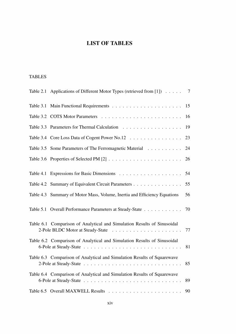
LIST OF TABLES

TABLES

Table 2.1 Applications of Different Motor Types (retrieved from [1]) . . . . . 7

Table 3.1 Main Functional Requirements . . . . . . . . . . . . . . . . . . . . 15

Table 3.2 COTS Motor Parameters . . . . . . . . . . . . . . . . . . . . . . . 16

Table 3.3 Parameters for Thermal Calculation . . . . . . . . . . . . . . . . . 19

Table 3.4 Core Loss Data of Cogent Power No.12 . . . . . . . . . . . . . . . 23

Table 3.5 Some Parameters of The Ferromagnetic Material . . . . . . . . . . 24

Table 3.6 Properties of Selected PM [2] . . . . . . . . . . . . . . . . . . . . . 26

Table 4.1 Expressions for Basic Dimensions . . . . . . . . . . . . . . . . . . 54

Table 4.2 Summary of Equivalent Circuit Parameters . . . . . . . . . . . . . . 55

Table 4.3 Summary of Motor Mass, Volume, Inertia and Efficiency Equations 56

Table 5.1 Overall Performance Parameters at Steady-State . . . . . . . . . . . 70

Table 6.1 Comparison of Analytical and Simulation Results of Sinusoidal2-Pole BLDC Motor at Steady-State . . . . . . . . . . . . . . . . . . . . 77

Table 6.2 Comparison of Analytical and Simulation Results of Sinusoidal6-Pole at Steady-State . . . . . . . . . . . . . . . . . . . . . . . . . . . . 81

Table 6.3 Comparison of Analytical and Simulation Results of Squarewave2-Pole at Steady-State . . . . . . . . . . . . . . . . . . . . . . . . . . . . 85

Table 6.4 Comparison of Analytical and Simulation Results of Squarewave6-Pole at Steady-State . . . . . . . . . . . . . . . . . . . . . . . . . . . . 89

Table 6.5 Overall MAXWELL Results . . . . . . . . . . . . . . . . . . . . . 90

xiv

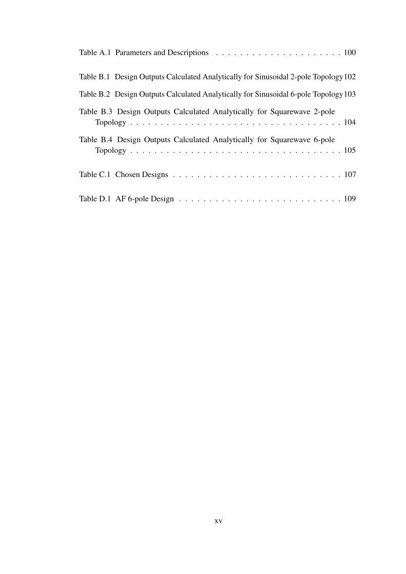
Table A.1 Parameters and Descriptions . . . . . . . . . . . . . . . . . . . . . 100

Table B.1 Design Outputs Calculated Analytically for Sinusoidal 2-pole Topology102

Table B.2 Design Outputs Calculated Analytically for Sinusoidal 6-pole Topology103

Table B.3 Design Outputs Calculated Analytically for Squarewave 2-poleTopology . . . . . . . . . . . . . . . . . . . . . . . . . . . . . . . . . . . 104

Table B.4 Design Outputs Calculated Analytically for Squarewave 6-poleTopology . . . . . . . . . . . . . . . . . . . . . . . . . . . . . . . . . . . 105

Table C.1 Chosen Designs . . . . . . . . . . . . . . . . . . . . . . . . . . . . 107

Table D.1 AF 6-pole Design . . . . . . . . . . . . . . . . . . . . . . . . . . . 109

xv

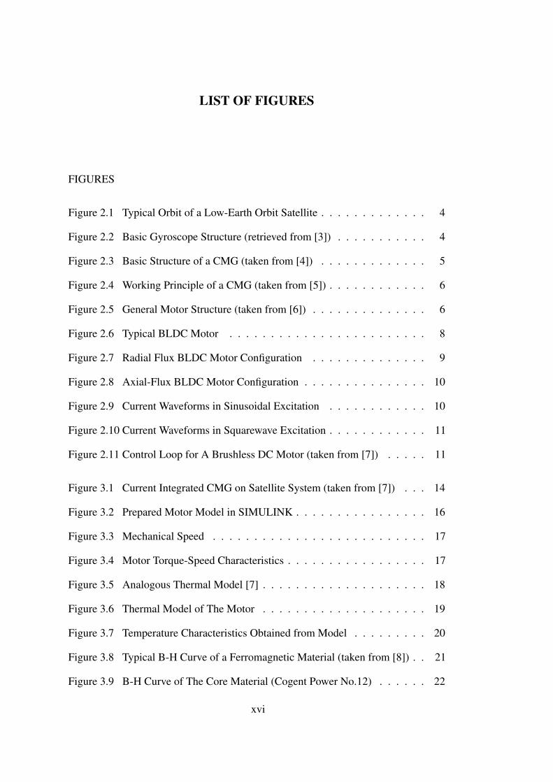
LIST OF FIGURES

FIGURES

Figure 2.1 Typical Orbit of a Low-Earth Orbit Satellite . . . . . . . . . . . . . 4

Figure 2.2 Basic Gyroscope Structure (retrieved from [3]) . . . . . . . . . . . 4

Figure 2.3 Basic Structure of a CMG (taken from [4]) . . . . . . . . . . . . . 5

Figure 2.4 Working Principle of a CMG (taken from [5]) . . . . . . . . . . . . 6

Figure 2.5 General Motor Structure (taken from [6]) . . . . . . . . . . . . . . 6

Figure 2.6 Typical BLDC Motor . . . . . . . . . . . . . . . . . . . . . . . . 8

Figure 2.7 Radial Flux BLDC Motor Configuration . . . . . . . . . . . . . . 9

Figure 2.8 Axial-Flux BLDC Motor Configuration . . . . . . . . . . . . . . . 10

Figure 2.9 Current Waveforms in Sinusoidal Excitation . . . . . . . . . . . . 10

Figure 2.10 Current Waveforms in Squarewave Excitation . . . . . . . . . . . . 11

Figure 2.11 Control Loop for A Brushless DC Motor (taken from [7]) . . . . . 11

Figure 3.1 Current Integrated CMG on Satellite System (taken from [7]) . . . 14

Figure 3.2 Prepared Motor Model in SIMULINK . . . . . . . . . . . . . . . . 16

Figure 3.3 Mechanical Speed . . . . . . . . . . . . . . . . . . . . . . . . . . 17

Figure 3.4 Motor Torque-Speed Characteristics . . . . . . . . . . . . . . . . . 17

Figure 3.5 Analogous Thermal Model [7] . . . . . . . . . . . . . . . . . . . . 18

Figure 3.6 Thermal Model of The Motor . . . . . . . . . . . . . . . . . . . . 19

Figure 3.7 Temperature Characteristics Obtained from Model . . . . . . . . . 20

Figure 3.8 Typical B-H Curve of a Ferromagnetic Material (taken from [8]) . . 21

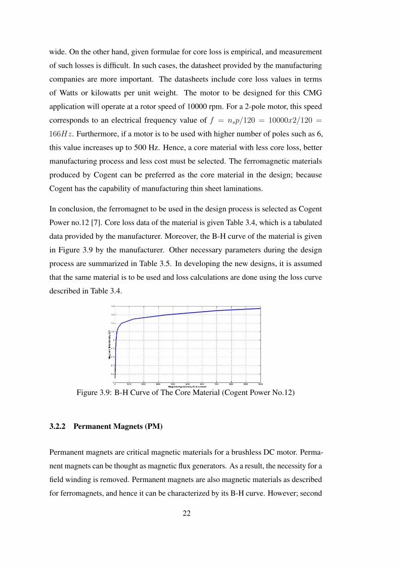
Figure 3.9 B-H Curve of The Core Material (Cogent Power No.12) . . . . . . 22

xvi

Figure 3.10 Demagnetization Curve of a PM . . . . . . . . . . . . . . . . . . . 24

Figure 3.11 Typical BLDC Motor (retrieved from [6]) . . . . . . . . . . . . . . 26

Figure 3.12 Magnetic Circuit of the BLDC Motor (retrieved from [6]) . . . . . 27

Figure 3.13 Simplified Magnetic Circuit (retrieved from [6]) . . . . . . . . . . 27

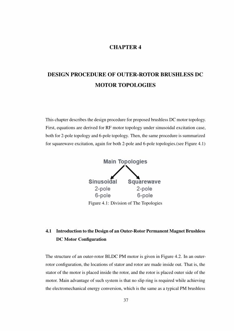
Figure 4.1 Division of The Topologies . . . . . . . . . . . . . . . . . . . . . 37

Figure 4.2 Structure of an Outer-Rotor BLDC Motor . . . . . . . . . . . . . . 38

Figure 4.3 Magnetic Circuit of Outer-Rotor BLDC Motor . . . . . . . . . . . 39

Figure 4.4 Equivalent Circuit of BLDC Motor (per phase) . . . . . . . . . . . 48

Figure 4.5 Typical Tooth-Slot Geometry . . . . . . . . . . . . . . . . . . . . 49

Figure 4.6 End Turn Geometry for Calculation of End-Turn Inductance . . . . 50

Figure 4.7 Volume Comparison of Designs Under Different Pole Numbers . . 57

Figure 4.8 Mass Comparison of Designs Under Different Pole Numbers . . . . 58

Figure 4.9 Inertia Comparison of Designs Under Different Pole Numbers . . . 58

Figure 4.10 Efficiency Comparison of Designs Under Different Pole Numbers . 59

Figure 4.11 Volume Comparison of Designs Under Different Excitation . . . . 59

Figure 4.12 Mass Comparison of Designs Under Different Excitation . . . . . . 60

Figure 4.13 Inertia Comparison of Designs Under Different Excitation . . . . . 60

Figure 4.14 Efficiency Comparison of Designs Under Different Excitation . . . 61

Figure 5.1 Tooth - Slot Dimensions . . . . . . . . . . . . . . . . . . . . . . . 64

Figure 5.2 Electrical Loading Variation with Increasing Ratio . . . . . . . . . 64

Figure 5.3 Analytical Results for Sinusoidal 2-pole Design . . . . . . . . . . . 65

Figure 5.4 Analytical Results for Sinusoidal 6-pole Design . . . . . . . . . . . 66

Figure 5.5 Analytical Results for Squarewave 2-pole Design . . . . . . . . . . 67

Figure 5.6 Analytical Results for Squarewave 6-pole Design . . . . . . . . . . 69

Figure 6.1 Simulation Model . . . . . . . . . . . . . . . . . . . . . . . . . . 72

xvii

Figure 6.2 Motor Model Prepared in MAXWELL (sinusoidal 2-pole) . . . . . 73

Figure 6.3 Magnetic Fields Obtained From MAXWELL for Sinusoidal 2-poleTopology . . . . . . . . . . . . . . . . . . . . . . . . . . . . . . . . . . . 74

Figure 6.4 Flux Density Along Air Gap and Tooth (sinusoidal 2-pole) . . . . . 74

Figure 6.5 Winding Current and Induced Voltage Obtained From MAXWELLfor Sinusoidal 2-pole Topology . . . . . . . . . . . . . . . . . . . . . . . 75

Figure 6.6 Torque and Speed Obtained From MAXWELL for Sinusoidal 2-pole Topology . . . . . . . . . . . . . . . . . . . . . . . . . . . . . . . . 76

Figure 6.7 Magnetic Fields Obtained From MAXWELL for Sinusoidal 6-poleTopology . . . . . . . . . . . . . . . . . . . . . . . . . . . . . . . . . . . 78

Figure 6.8 Flux Density Along Air Gap and Tooth (sinusoidal 6-pole) . . . . . 78

Figure 6.9 Winding Current and Induced Voltage Obtained From MAXWELLfor Sinusoidal 6-pole Topology . . . . . . . . . . . . . . . . . . . . . . . 79

Figure 6.10 Torque and Speed Obtained From MAXWELL for Sinusoidal 6-pole Topology . . . . . . . . . . . . . . . . . . . . . . . . . . . . . . . . 80

Figure 6.11 Magnetic Fields Obtained in MAXWELL for Squarewave 2-poleTopology . . . . . . . . . . . . . . . . . . . . . . . . . . . . . . . . . . . 82

Figure 6.12 Flux Density Along Air Gap and Tooth (squarewave 2-pole) . . . . 82

Figure 6.13 Winding Current and Induced Voltage Obtained From MAXWELLfor Squarewave 2-pole Topology . . . . . . . . . . . . . . . . . . . . . . 83

Figure 6.14 Torque and Speed Obtained From MAXWELL for Squarewave2-pole Topology . . . . . . . . . . . . . . . . . . . . . . . . . . . . . . . 84

Figure 6.15 Magnetic Fields Obtained in MAXWELL for Squarewave 6-poleTopology . . . . . . . . . . . . . . . . . . . . . . . . . . . . . . . . . . . 86

Figure 6.16 Flux Density Along Air Gap and Tooth (squarewave 6-pole) . . . . 86

Figure 6.17 Winding Current and Induced Voltage Obtained From MAXWELLfor Squarewave 6-pole Topology . . . . . . . . . . . . . . . . . . . . . . 87

Figure 6.18 Torque and Speed Obtained From MAXWELL for Squarewave6-pole Topology . . . . . . . . . . . . . . . . . . . . . . . . . . . . . . . 88

Figure 6.19 Magnetic Fields Obtained in MAXWELL for AF Squarewave 6-pole Topology . . . . . . . . . . . . . . . . . . . . . . . . . . . . . . . . 89

xviii

Figure 6.20 Parameters Obtained From MAXWELL for AF Squarewave 6-poleTopology . . . . . . . . . . . . . . . . . . . . . . . . . . . . . . . . . . . 90

Figure 7.1 Overall Volume Comparison of Chosen Designs . . . . . . . . . . 92

Figure 7.2 Overall Mass Comparison of Chosen Designs . . . . . . . . . . . . 92

Figure 7.3 Overall Inertia Comparison of Chosen Designs . . . . . . . . . . . 93

Figure 7.4 Overall Efficiency Comparison of Chosen Design . . . . . . . . . . 93

xix

LIST OF ABBREVIATIONS

AF Axial Flux

BLDC Brushless DC

CMG Control Moment Gyroscope

COTS Commercial off-the-shelf

DC Direct Current

emf Electromotive Force

FEA Finite-Element Analysis

LEO Low Earth Orbit

PM Permanent Magnet

RF Radial Flux

rms Root-Mean-Square

xx

CHAPTER 1

INTRODUCTION

1.1 Scope of Thesis

Actuating systems are widely used in aerospace applications, as well as other consumer

electronic systems or other household applications. In an actuating system within an

aerospace application such as satellites, brushless DC motors are coupled with the

momentum wheel and play an important role in controlling these systems in order to

stabilize and give required maneuver to the whole system.

This thesis study mainly focuses on the conventional brushless direct-current (DC) mo-

tors used in such applications and proposes certain outer-rotor topologies and discusses

the strengths and weaknesses between each other in terms of torque characteristics per

unit volume and mass, efficiency, and inertia.

1.2 Outline of Thesis

This thesis is divided into six main chapters,except from this chapter, and each of

which focuses on a certain topic as a milestone.

Chapter 2 presents the fundamentals of a typical control moment gyroscope actuating

system configuration and electrical motors used in these systems. Furthermore, the

electrical motor to be designed is presented such that types of the electrical motors are

stated.

Chapter 3 defines the main problem in current control moment gyroscope (CMG) sys-

1

tems and major requirements related to the wheel motors are stated. Then, fundamental

concepts related to permanent magnet brushless DC motors are defined. In this manner,

magnetic circuit characteristics and specific torque equations relating basic sizes of the

motors that will be used throughout the study are presented in corresponding sections.

Chapter 4 states the design of the proposed outer-rotor brushless DC motor topologies,

derives the main expressions used throughout the design process. Changes in the

design both for pole numbers and excitation such as squarewave or sinusoidal are

presented.

Chapter 5 presents the results and makes discussions on these results. Main advantages

and disadvantages of each design is discussed.

Chapter 6 presents the results obtained in a finite-element analysis tool in order to

verify the analytical results.

Chapter 7 concludes the thesis by summarizing the overall study and stating a brief

future work.

2

CHAPTER 2

ACTUATING SYSTEMS IN LEO SATELLITES AND TYPICAL

ELECTRICAL MOTORS

2.1 General Overview

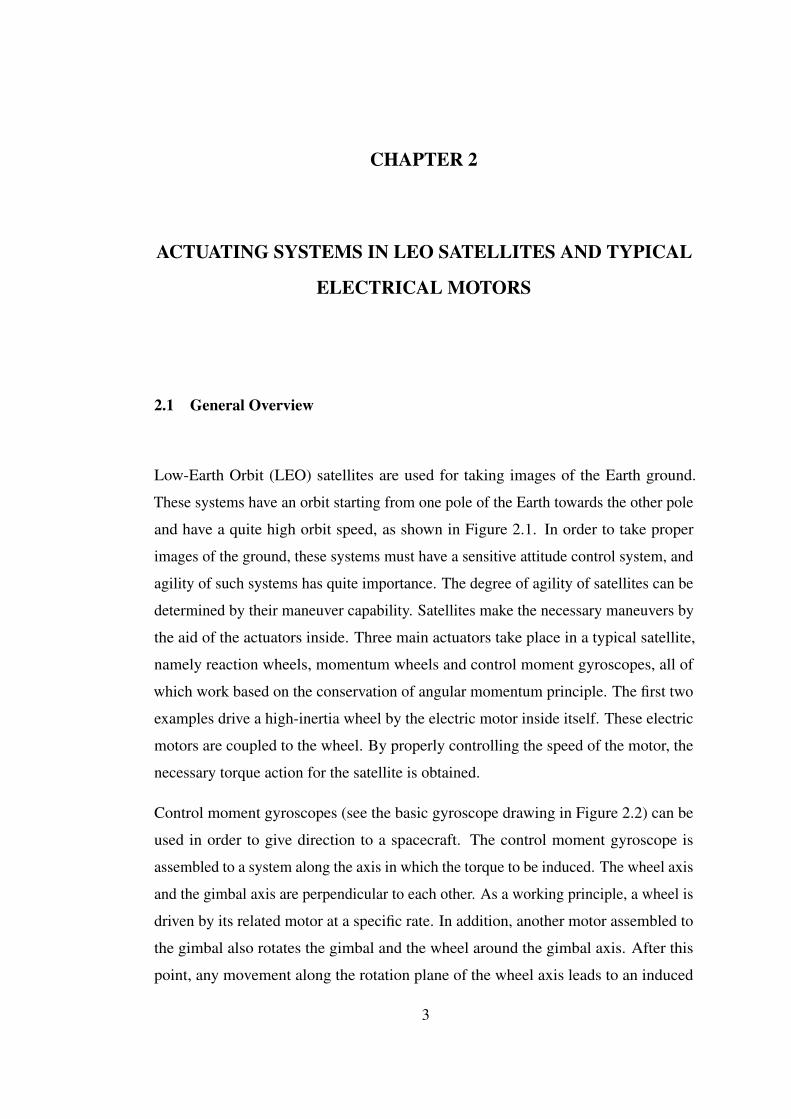
Low-Earth Orbit (LEO) satellites are used for taking images of the Earth ground.

These systems have an orbit starting from one pole of the Earth towards the other pole

and have a quite high orbit speed, as shown in Figure 2.1. In order to take proper

images of the ground, these systems must have a sensitive attitude control system, and

agility of such systems has quite importance. The degree of agility of satellites can be

determined by their maneuver capability. Satellites make the necessary maneuvers by

the aid of the actuators inside. Three main actuators take place in a typical satellite,

namely reaction wheels, momentum wheels and control moment gyroscopes, all of

which work based on the conservation of angular momentum principle. The first two

examples drive a high-inertia wheel by the electric motor inside itself. These electric

motors are coupled to the wheel. By properly controlling the speed of the motor, the

necessary torque action for the satellite is obtained.

Control moment gyroscopes (see the basic gyroscope drawing in Figure 2.2) can be

used in order to give direction to a spacecraft. The control moment gyroscope is

assembled to a system along the axis in which the torque to be induced. The wheel axis

and the gimbal axis are perpendicular to each other. As a working principle, a wheel is

driven by its related motor at a specific rate. In addition, another motor assembled to

the gimbal also rotates the gimbal and the wheel around the gimbal axis. After this

point, any movement along the rotation plane of the wheel axis leads to an induced

3

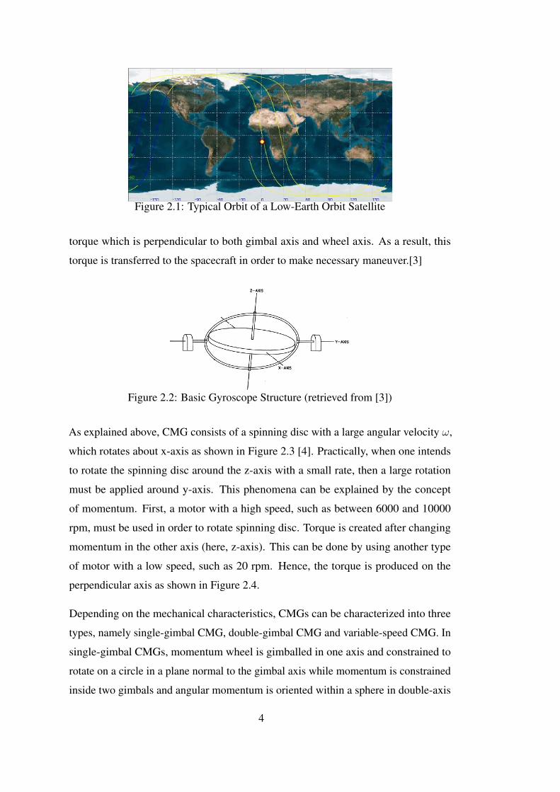
Figure 2.1: Typical Orbit of a Low-Earth Orbit Satellite

torque which is perpendicular to both gimbal axis and wheel axis. As a result, this

torque is transferred to the spacecraft in order to make necessary maneuver.[3]

Figure 2.2: Basic Gyroscope Structure (retrieved from [3])

As explained above, CMG consists of a spinning disc with a large angular velocity ω,

which rotates about x-axis as shown in Figure 2.3 [4]. Practically, when one intends

to rotate the spinning disc around the z-axis with a small rate, then a large rotation

must be applied around y-axis. This phenomena can be explained by the concept

of momentum. First, a motor with a high speed, such as between 6000 and 10000

rpm, must be used in order to rotate spinning disc. Torque is created after changing

momentum in the other axis (here, z-axis). This can be done by using another type

of motor with a low speed, such as 20 rpm. Hence, the torque is produced on the

perpendicular axis as shown in Figure 2.4.

Depending on the mechanical characteristics, CMGs can be characterized into three

types, namely single-gimbal CMG, double-gimbal CMG and variable-speed CMG. In

single-gimbal CMGs, momentum wheel is gimballed in one axis and constrained to

rotate on a circle in a plane normal to the gimbal axis while momentum is constrained

inside two gimbals and angular momentum is oriented within a sphere in double-axis

4

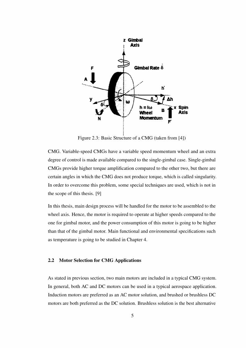
Figure 2.3: Basic Structure of a CMG (taken from [4])

CMG. Variable-speed CMGs have a variable speed momentum wheel and an extra

degree of control is made available compared to the single-gimbal case. Single-gimbal

CMGs provide higher torque amplification compared to the other two, but there are

certain angles in which the CMG does not produce torque, which is called singularity.

In order to overcome this problem, some special techniques are used, which is not in

the scope of this thesis. [9]

In this thesis, main design process will be handled for the motor to be assembled to the

wheel axis. Hence, the motor is required to operate at higher speeds compared to the

one for gimbal motor, and the power consumption of this motor is going to be higher

than that of the gimbal motor. Main functional and environmental specifications such

as temperature is going to be studied in Chapter 4.

2.2 Motor Selection for CMG Applications

As stated in previous section, two main motors are included in a typical CMG system.

In general, both AC and DC motors can be used in a typical aerospace application.

Induction motors are preferred as an AC motor solution, and brushed or brushless DC

motors are both preferred as the DC solution. Brushless solution is the best alternative

5

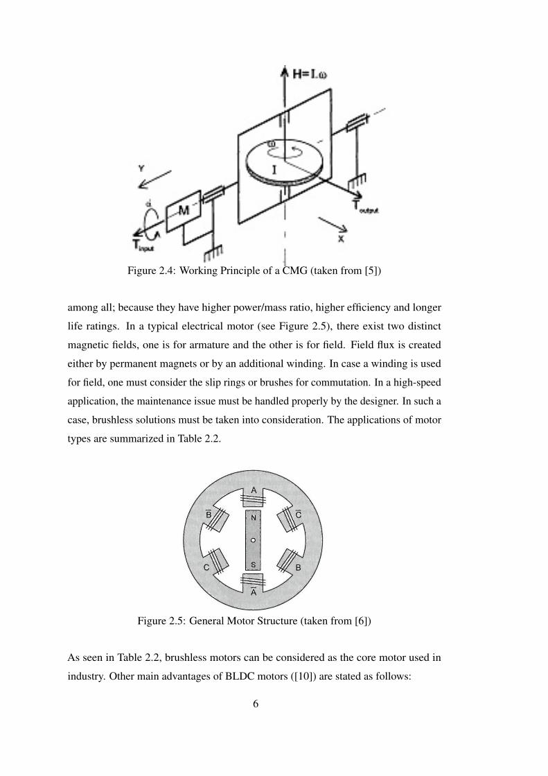
Figure 2.4: Working Principle of a CMG (taken from [5])

among all; because they have higher power/mass ratio, higher efficiency and longer

life ratings. In a typical electrical motor (see Figure 2.5), there exist two distinct

magnetic fields, one is for armature and the other is for field. Field flux is created

either by permanent magnets or by an additional winding. In case a winding is used

for field, one must consider the slip rings or brushes for commutation. In a high-speed

application, the maintenance issue must be handled properly by the designer. In such a

case, brushless solutions must be taken into consideration. The applications of motor

types are summarized in Table 2.2.

Figure 2.5: General Motor Structure (taken from [6])

As seen in Table 2.2, brushless motors can be considered as the core motor used in

industry. Other main advantages of BLDC motors ([10]) are stated as follows:

6

Table 2.1: Applications of Different Motor Types (retrieved from [1])

AC Induction Motors Brushed DC Motors Brushless DC Motors Stepper MotorsThrust Vector ControlApplications

Limited Life-Time Ap-plications

Thrust Vector ControlApplications

Optical Drives

High-Torque and High-rpm Applications

Low-rpm Applications Fuel Valve Control Ac-tuators

Solar Array Deploy-ment

High-Torque Applica-tions

Solar Array Deploy-ment

Gimbal Positioning

Control Moment Gyro-scopes

Low-Torque Applica-tions

High-rpm Applications Open-Loop Micro Posi-tioning

Light Weight Applica-tions

Timer Switching

Low Thermal EmissionApplications

• High speed which may increase up to 100.000 rpm

• High torque at high speeds

• Higher torque ratings (about double) when compared to brushed DC motor

equivalents with same size

• No winding on rotor, improvement on heat dissipation

• No brushes, no high maintenance cost

• Higher efficiency

• Vacuum compatible

On the other hand, the disadvantages of using a brushless DC motor in an aerospace

application may be counted as relatively higher electronic cost and increase in com-

plexity of the drive circuitry. [10] As a whole, brushless DC motors are preferred

as an electrical motor solution at all applications in industry, as well as aerospace

applications.

7

2.3 General Overview of Brushless DC Motors

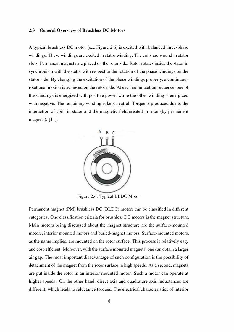
A typical brushless DC motor (see Figure 2.6) is excited with balanced three-phase

windings. These windings are excited in stator winding. The coils are wound in stator

slots. Permanent magnets are placed on the rotor side. Rotor rotates inside the stator in

synchronism with the stator with respect to the rotation of the phase windings on the

stator side. By changing the excitation of the phase windings properly, a continuous

rotational motion is achieved on the rotor side. At each commutation sequence, one of

the windings is energized with positive power while the other winding is energized

with negative. The remaining winding is kept neutral. Torque is produced due to the

interaction of coils in stator and the magnetic field created in rotor (by permanent

magnets). [11].

Figure 2.6: Typical BLDC Motor

Permanent magnet (PM) brushless DC (BLDC) motors can be classified in different

categories. One classification criteria for brushless DC motors is the magnet structure.

Main motors being discussed about the magnet structure are the surface-mounted

motors, interior mounted motors and buried-magnet motors. Surface-mounted motors,

as the name implies, are mounted on the rotor surface. This process is relatively easy

and cost-efficient. Moreover, with the surface mounted magnets, one can obtain a larger

air gap. The most important disadvantage of such configuration is the possibility of

detachment of the magnet from the rotor surface in high speeds. As a second, magnets

are put inside the rotor in an interior mounted motor. Such a motor can operate at

higher speeds. On the other hand, direct axis and quadrature axis inductances are

different, which leads to reluctance torques. The electrical characteristics of interior

8

motors and the buried-magnet motors are equivalent.

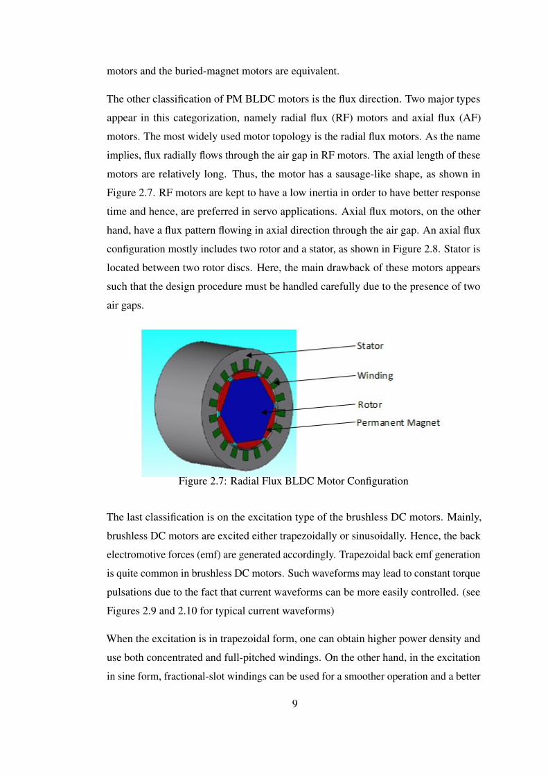
The other classification of PM BLDC motors is the flux direction. Two major types

appear in this categorization, namely radial flux (RF) motors and axial flux (AF)

motors. The most widely used motor topology is the radial flux motors. As the name

implies, flux radially flows through the air gap in RF motors. The axial length of these

motors are relatively long. Thus, the motor has a sausage-like shape, as shown in

Figure 2.7. RF motors are kept to have a low inertia in order to have better response

time and hence, are preferred in servo applications. Axial flux motors, on the other

hand, have a flux pattern flowing in axial direction through the air gap. An axial flux

configuration mostly includes two rotor and a stator, as shown in Figure 2.8. Stator is

located between two rotor discs. Here, the main drawback of these motors appears

such that the design procedure must be handled carefully due to the presence of two

air gaps.

Figure 2.7: Radial Flux BLDC Motor Configuration

The last classification is on the excitation type of the brushless DC motors. Mainly,

brushless DC motors are excited either trapezoidally or sinusoidally. Hence, the back

electromotive forces (emf) are generated accordingly. Trapezoidal back emf generation

is quite common in brushless DC motors. Such waveforms may lead to constant torque

pulsations due to the fact that current waveforms can be more easily controlled. (see

Figures 2.9 and 2.10 for typical current waveforms)

When the excitation is in trapezoidal form, one can obtain higher power density and

use both concentrated and full-pitched windings. On the other hand, in the excitation

in sine form, fractional-slot windings can be used for a smoother operation and a better

9

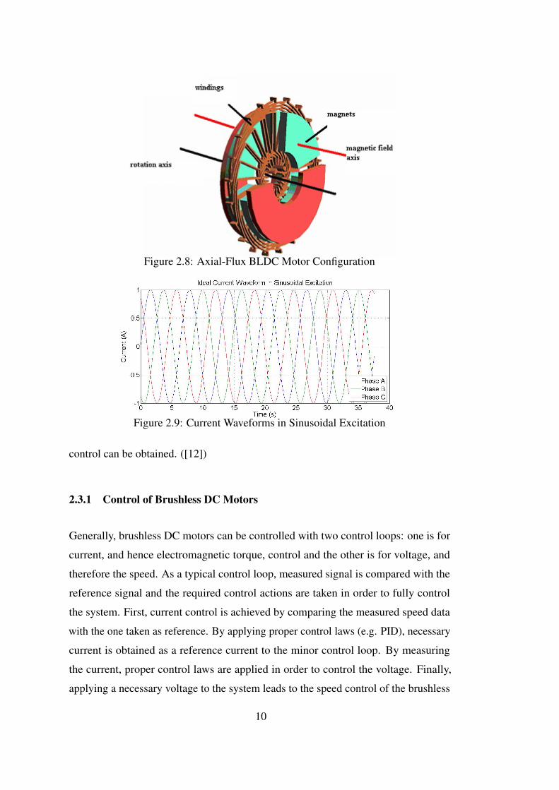
Figure 2.8: Axial-Flux BLDC Motor Configuration

Figure 2.9: Current Waveforms in Sinusoidal Excitation

control can be obtained. ([12])

2.3.1 Control of Brushless DC Motors

Generally, brushless DC motors can be controlled with two control loops: one is for

current, and hence electromagnetic torque, control and the other is for voltage, and

therefore the speed. As a typical control loop, measured signal is compared with the

reference signal and the required control actions are taken in order to fully control

the system. First, current control is achieved by comparing the measured speed data

with the one taken as reference. By applying proper control laws (e.g. PID), necessary

current is obtained as a reference current to the minor control loop. By measuring

the current, proper control laws are applied in order to control the voltage. Finally,

applying a necessary voltage to the system leads to the speed control of the brushless

10

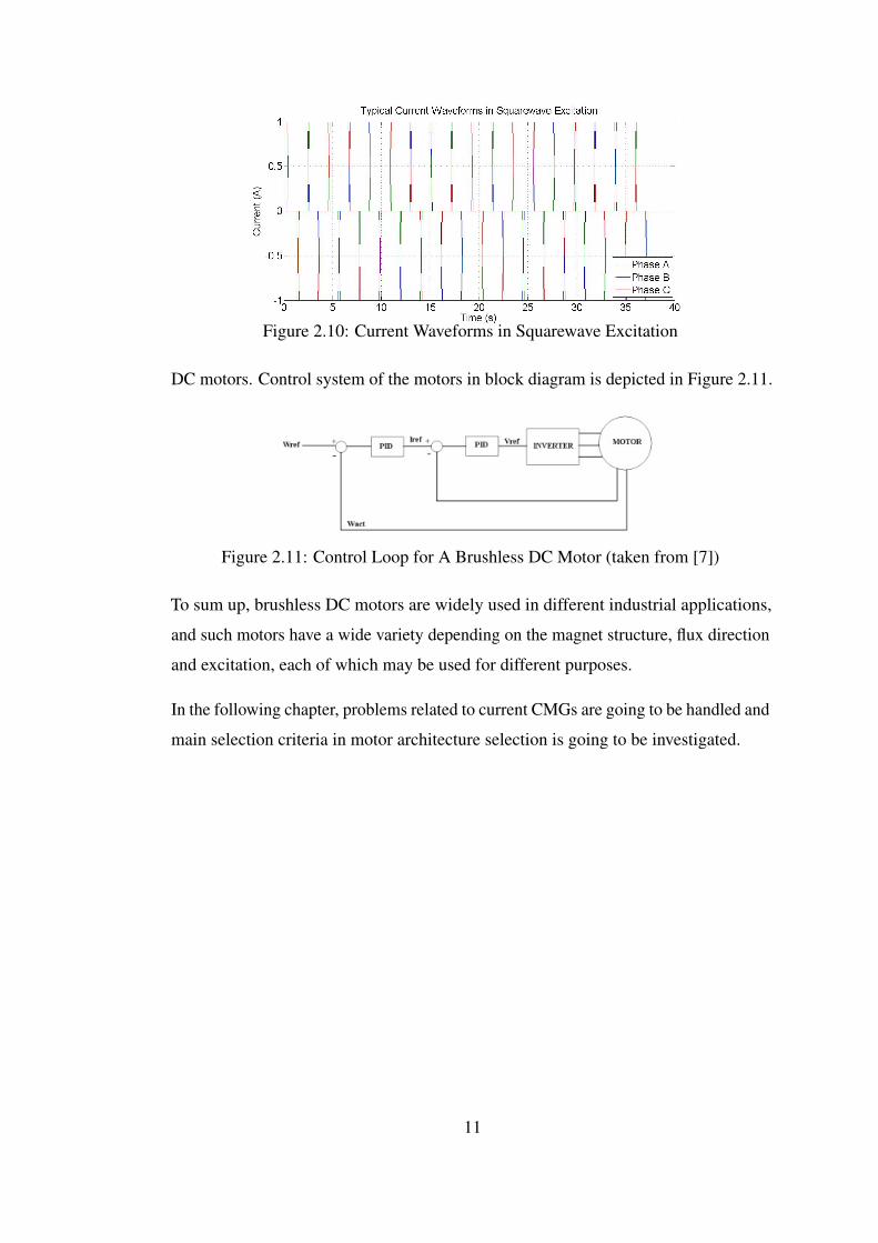
Figure 2.10: Current Waveforms in Squarewave Excitation

DC motors. Control system of the motors in block diagram is depicted in Figure 2.11.

Figure 2.11: Control Loop for A Brushless DC Motor (taken from [7])

To sum up, brushless DC motors are widely used in different industrial applications,

and such motors have a wide variety depending on the magnet structure, flux direction

and excitation, each of which may be used for different purposes.

In the following chapter, problems related to current CMGs are going to be handled and

main selection criteria in motor architecture selection is going to be investigated.

11

12

CHAPTER 3

PROBLEM DEFINITION AND MOTOR ARCHITECTURE

SELECTION

This chapter first states the problem in existing CMG motors and define the main

requirements and then, general expressions are derived for conventional BLDC motors.

Here, the term "conventional" is used for the topology, where the stator is located

outside the motor and the excitation is made, while the rotor is located inside the motor

where the mechanical power is obtained.

3.1 Problem Definition and The Requirements

3.1.1 Problem Definition

In this thesis, the BLDC motor to be designed is for the wheel motor. Wheel motor

operates at a relatively high constant speed, which is in the order of 10000 rpm. An

acceleration time between 1 and 2 minutes will be taken into consideration and friction

and windage torque components due to bearings will be investigated.

For CMG prototypes, commercial off-the-shelf (COTS) motor designs are being used.

This leads to the necessity of a new design; because COTS products are manufactured

as sausage-type BLDC motors. As a wheel motor, the inertia contribution of such a

design is relatively low. On the contrary, more inertia contribution is made for the

gimbal motor, which in turn leads to an increase in the power consumption of the

gimbal motor. Due to the fact that it is a sausage-type, the load must be coupled to

the motor with an external coupling. Furthermore, the distance between bearings are

13

relatively high; hence balancing problems may occur in such designs.

The second problem is the compatibility issues between the COTS design and the

requirements. For a motor design to be used in such applications, the major disturbance

component is the friction torque between shaft and bearings. Commercial motors

are usually designed for dynamic load conditions, which may make these designs

over-safe and over-designed, which in turn leads to an increase in mass or volume.

Hence, a motor must be designed to fulfill the requirements with total correspondence.

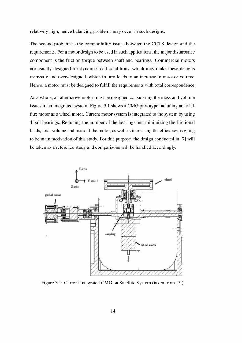
As a whole, an alternative motor must be designed considering the mass and volume

issues in an integrated system. Figure 3.1 shows a CMG prototype including an axial-

flux motor as a wheel motor. Current motor system is integrated to the system by using

4 ball bearings. Reducing the number of the bearings and minimizing the frictional

loads, total volume and mass of the motor, as well as increasing the efficiency is going

to be main motivation of this study. For this purpose, the design conducted in [7] will

be taken as a reference study and comparisons will be handled accordingly.

Figure 3.1: Current Integrated CMG on Satellite System (taken from [7])

14

3.1.2 Requirements

3.1.2.1 Functional Requirements

Functional requirements are derived from the requirements from the system-level

requirements. An existing CMG has a total wheel inertia of 4.83x10−4kg.m2. The

motor to be designed is desired to have an inertia as large as possible due to the fact that

it is desired to have a large inertia contribution to the total wheel system. In addition,

rotation of the wheel motor with a rate of 10.000 rpm is defined. Finally, accelerating

the wheel system in between 35 and 120 seconds is set to be as the acceleration time.

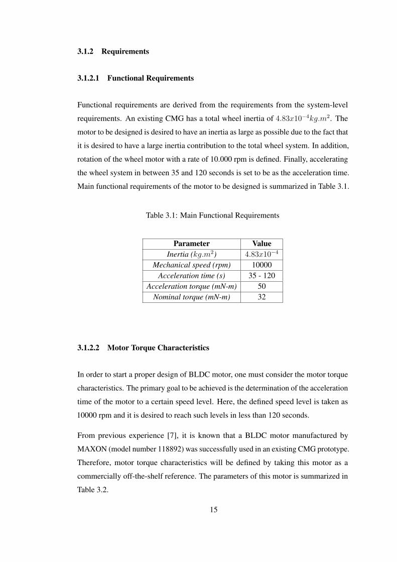
Main functional requirements of the motor to be designed is summarized in Table 3.1.

Table 3.1: Main Functional Requirements

Parameter ValueInertia (kg.m2) 4.83x10−4

Mechanical speed (rpm) 10000Acceleration time (s) 35 - 120

Acceleration torque (mN-m) 50Nominal torque (mN-m) 32

3.1.2.2 Motor Torque Characteristics

In order to start a proper design of BLDC motor, one must consider the motor torque

characteristics. The primary goal to be achieved is the determination of the acceleration

time of the motor to a certain speed level. Here, the defined speed level is taken as

10000 rpm and it is desired to reach such levels in less than 120 seconds.

From previous experience [7], it is known that a BLDC motor manufactured by

MAXON (model number 118892) was successfully used in an existing CMG prototype.

Therefore, motor torque characteristics will be defined by taking this motor as a

commercially off-the-shelf reference. The parameters of this motor is summarized in

Table 3.2.

15

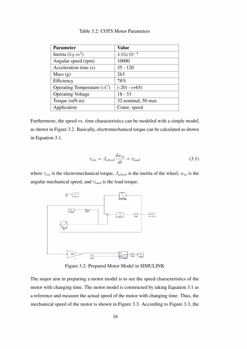
Table 3.2: COTS Motor Parameters

Parameter ValueInertia (kg.m2) 4.83x10−4

Angular speed (rpm) 10000Acceleration time (s) 35 - 120Mass (g) 263Efficiency 78%Operating Temperature (C) (-20) - (+65)Operating Voltage 18 - 33Torque (mN.m) 32 nominal, 50 maxApplication Const. speed

Furthermore, the speed vs. time characteristics can be modeled with a simple model,

as shown in Figure 3.2. Basically, electromechanical torque can be calculated as shown

in Equation 3.1.

τem = Jwheeldwmdt

+ τload (3.1)

where τem is the electromechanical torque, Jwheel is the inertia of the wheel, wm is the

angular mechanical speed, and τload is the load torque.

Figure 3.2: Prepared Motor Model in SIMULINK

The major aim in preparing a motor model is to see the speed characteristics of the

motor with changing time. The motor model is constructed by taking Equation 3.1 as

a reference and measure the actual speed of the motor with changing time. Thus, the

mechanical speed of the motor is shown in Figure 3.3. According to Figure 3.3, the

16

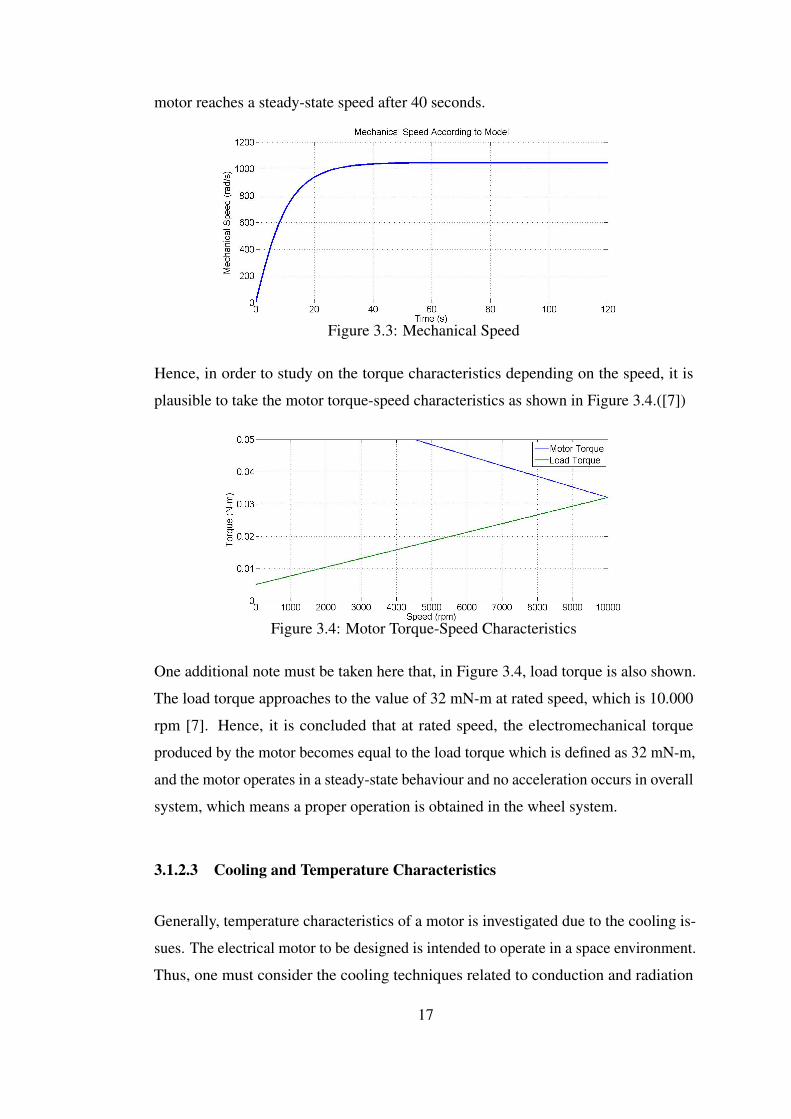
motor reaches a steady-state speed after 40 seconds.

Figure 3.3: Mechanical Speed

Hence, in order to study on the torque characteristics depending on the speed, it is

plausible to take the motor torque-speed characteristics as shown in Figure 3.4.([7])

Figure 3.4: Motor Torque-Speed Characteristics

One additional note must be taken here that, in Figure 3.4, load torque is also shown.

The load torque approaches to the value of 32 mN-m at rated speed, which is 10.000

rpm [7]. Hence, it is concluded that at rated speed, the electromechanical torque

produced by the motor becomes equal to the load torque which is defined as 32 mN-m,

and the motor operates in a steady-state behaviour and no acceleration occurs in overall

system, which means a proper operation is obtained in the wheel system.

3.1.2.3 Cooling and Temperature Characteristics

Generally, temperature characteristics of a motor is investigated due to the cooling is-

sues. The electrical motor to be designed is intended to operate in a space environment.

Thus, one must consider the cooling techniques related to conduction and radiation

17

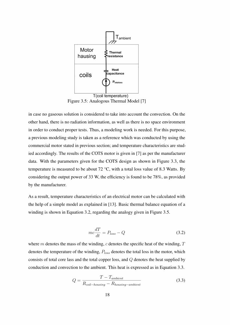
Figure 3.5: Analogous Thermal Model [7]

in case no gaseous solution is considered to take into account the convection. On the

other hand, there is no radiation information, as well as there is no space environment

in order to conduct proper tests. Thus, a modeling work is needed. For this purpose,

a previous modeling study is taken as a reference which was conducted by using the

commercial motor stated in previous section; and temperature characteristics are stud-

ied accordingly. The results of the COTS motor is given in [7] as per the manufacturer

data. With the parameters given for the COTS design as shown in Figure 3.3, the

temperature is measured to be about 72 °C, with a total loss value of 8.3 Watts. By

considering the output power of 33 W, the efficiency is found to be 78%, as provided

by the manufacturer.

As a result, temperature characteristics of an electrical motor can be calculated with

the help of a simple model as explained in [13]. Basic thermal balance equation of a

winding is shown in Equation 3.2, regarding the analogy given in Figure 3.5.

mcdT

dt= Ploss −Q (3.2)

where m denotes the mass of the winding, c denotes the specific heat of the winding, T

denotes the temperature of the winding, Ploss denotes the total loss in the motor, which

consists of total core lass and the total copper loss, and Q denotes the heat supplied by

conduction and convection to the ambient. This heat is expressed as in Equation 3.3.

Q =T − Tambient

Rcoil−housing −Rhousing−ambient(3.3)

18

Here, Tambient denotes the ambient temperature, Rcoil−housing is the thermal resistance

between coils and housing and Rhousing−ambient is thermal resistance between housing

and ambient. Copper losses and core losses are to be calculated in Chapter 4, and

the necessary values are taken from there by calculating all performance parameters

such as current as phase resistance. Hence, total losses are taken as 3.55 Watts. Total

copper weight is calculated as 163 grams. Other parameters are shown in Table 3.3.

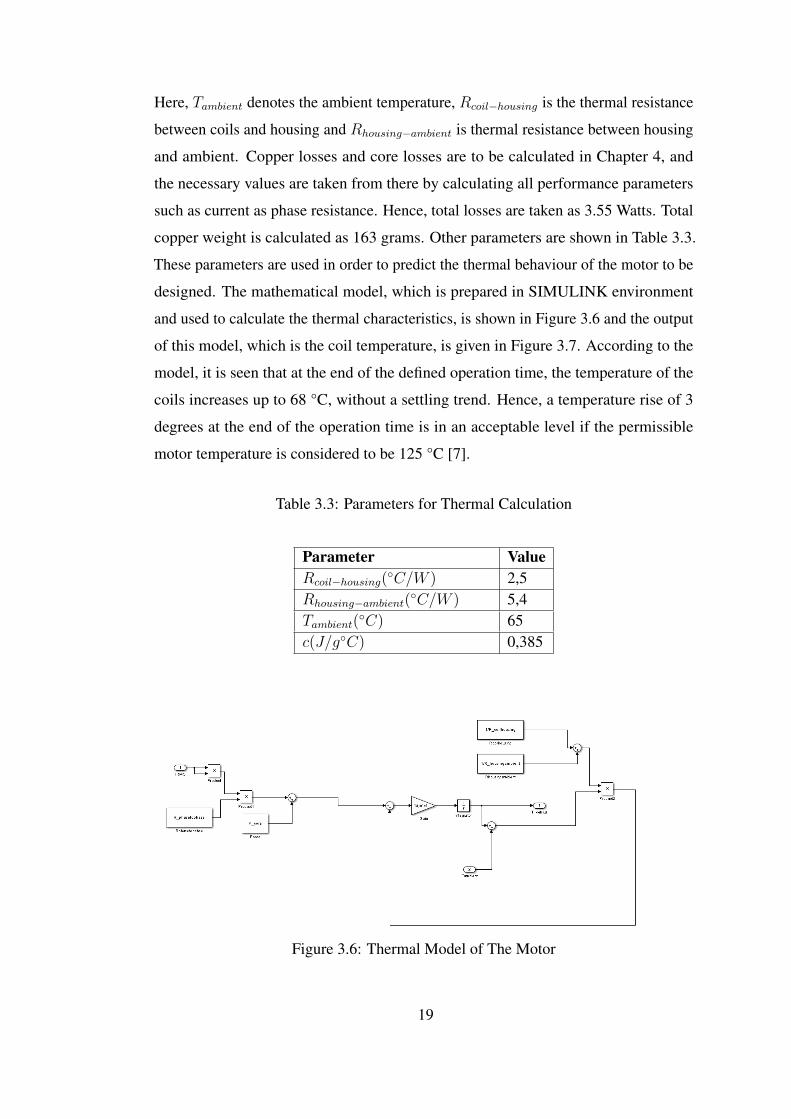
These parameters are used in order to predict the thermal behaviour of the motor to be

designed. The mathematical model, which is prepared in SIMULINK environment

and used to calculate the thermal characteristics, is shown in Figure 3.6 and the output

of this model, which is the coil temperature, is given in Figure 3.7. According to the

model, it is seen that at the end of the defined operation time, the temperature of the

coils increases up to 68 °C, without a settling trend. Hence, a temperature rise of 3

degrees at the end of the operation time is in an acceptable level if the permissible

motor temperature is considered to be 125 °C [7].

Table 3.3: Parameters for Thermal Calculation

Parameter ValueRcoil−housing(

C/W ) 2,5Rhousing−ambient(

C/W ) 5,4Tambient(

C) 65c(J/gC) 0,385

Figure 3.6: Thermal Model of The Motor

19

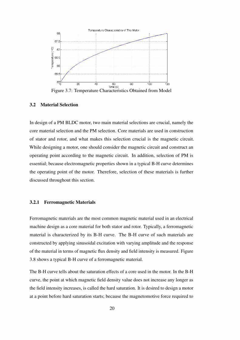
Figure 3.7: Temperature Characteristics Obtained from Model

3.2 Material Selection

In design of a PM BLDC motor, two main material selections are crucial, namely the

core material selection and the PM selection. Core materials are used in construction

of stator and rotor, and what makes this selection crucial is the magnetic circuit.

While designing a motor, one should consider the magnetic circuit and construct an

operating point according to the magnetic circuit. In addition, selection of PM is

essential; because electromagnetic properties shown in a typical B-H curve determines

the operating point of the motor. Therefore, selection of these materials is further

discussed throughout this section.

3.2.1 Ferromagnetic Materials

Ferromagnetic materials are the most common magnetic material used in an electrical

machine design as a core material for both stator and rotor. Typically, a ferromagnetic

material is characterized by its B-H curve. The B-H curve of such materials are

constructed by applying sinusoidal excitation with varying amplitude and the response

of the material in terms of magnetic flux density and field intensity is measured. Figure

3.8 shows a typical B-H curve of a ferromagnetic material.

The B-H curve tells about the saturation effects of a core used in the motor. In the B-H

curve, the point at which magnetic field density value does not increase any longer as

the field intensity increases, is called the hard saturation. It is desired to design a motor

at a point before hard saturation starts; because the magnetomotive force required to

20

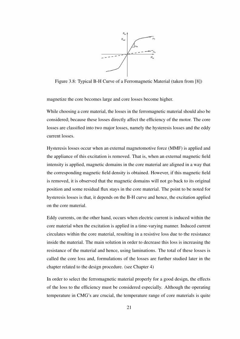
Figure 3.8: Typical B-H Curve of a Ferromagnetic Material (taken from [8])

magnetize the core becomes large and core losses become higher.

While choosing a core material, the losses in the ferromagnetic material should also be

considered; because these losses directly affect the efficiency of the motor. The core

losses are classified into two major losses, namely the hysteresis losses and the eddy

current losses.

Hysteresis losses occur when an external magnetomotive force (MMF) is applied and

the appliance of this excitation is removed. That is, when an external magnetic field

intensity is applied, magnetic domains in the core material are aligned in a way that

the corresponding magnetic field density is obtained. However, if this magnetic field

is removed, it is observed that the magnetic domains will not go back to its original

position and some residual flux stays in the core material. The point to be noted for

hysteresis losses is that, it depends on the B-H curve and hence, the excitation applied

on the core material.

Eddy currents, on the other hand, occurs when electric current is induced within the

core material when the excitation is applied in a time-varying manner. Induced current

circulates within the core material, resulting in a resistive loss due to the resistance

inside the material. The main solution in order to decrease this loss is increasing the

resistance of the material and hence, using laminations. The total of these losses is

called the core loss and, formulations of the losses are further studied later in the

chapter related to the design procedure. (see Chapter 4)

In order to select the ferromagnetic material properly for a good design, the effects

of the loss to the efficiency must be considered especially. Although the operating

temperature in CMG’s are crucial, the temperature range of core materials is quite

21

wide. On the other hand, given formulae for core loss is empirical, and measurement

of such losses is difficult. In such cases, the datasheet provided by the manufacturing

companies are more important. The datasheets include core loss values in terms

of Watts or kilowatts per unit weight. The motor to be designed for this CMG

application will operate at a rotor speed of 10000 rpm. For a 2-pole motor, this speed

corresponds to an electrical frequency value of f = nsp/120 = 10000x2/120 =

166Hz. Furthermore, if a motor is to be used with higher number of poles such as 6,

this value increases up to 500 Hz. Hence, a core material with less core loss, better

manufacturing process and less cost must be selected. The ferromagnetic materials

produced by Cogent can be preferred as the core material in the design; because

Cogent has the capability of manufacturing thin sheet laminations.

In conclusion, the ferromagnet to be used in the design process is selected as Cogent

Power no.12 [7]. Core loss data of the material is given Table 3.4, which is a tabulated

data provided by the manufacturer. Moreover, the B-H curve of the material is given

in Figure 3.9 by the manufacturer. Other necessary parameters during the design

process are summarized in Table 3.5. In developing the new designs, it is assumed

that the same material is to be used and loss calculations are done using the loss curve

described in Table 3.4.

Figure 3.9: B-H Curve of The Core Material (Cogent Power No.12)

3.2.2 Permanent Magnets (PM)

Permanent magnets are critical magnetic materials for a brushless DC motor. Perma-

nent magnets can be thought as magnetic flux generators. As a result, the necessity for a

field winding is removed. Permanent magnets are also magnetic materials as described

for ferromagnets, and hence it can be characterized by its B-H curve. However; second

22

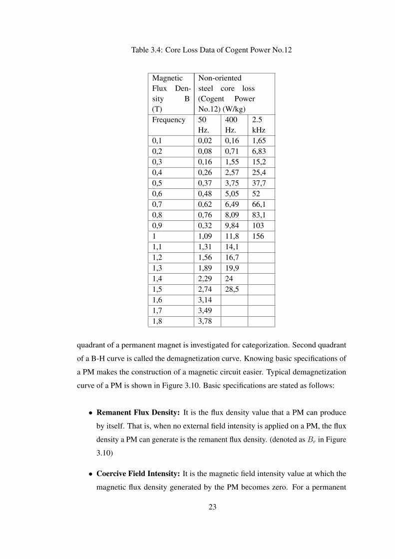
Table 3.4: Core Loss Data of Cogent Power No.12

MagneticFlux Den-sity B(T)

Non-orientedsteel core loss(Cogent PowerNo.12) (W/kg)

Frequency 50Hz.

400Hz.

2.5kHz

0,1 0,02 0,16 1,650,2 0,08 0,71 6,830,3 0,16 1,55 15,20,4 0,26 2,57 25,40,5 0,37 3,75 37,70,6 0,48 5,05 520,7 0,62 6,49 66,10,8 0,76 8,09 83,10,9 0,32 9,84 1031 1,09 11,8 1561,1 1,31 14,11,2 1,56 16,71,3 1,89 19,91,4 2,29 241,5 2,74 28,51,6 3,141,7 3,491,8 3,78

quadrant of a permanent magnet is investigated for categorization. Second quadrant

of a B-H curve is called the demagnetization curve. Knowing basic specifications of

a PM makes the construction of a magnetic circuit easier. Typical demagnetization

curve of a PM is shown in Figure 3.10. Basic specifications are stated as follows:

• Remanent Flux Density: It is the flux density value that a PM can produce

by itself. That is, when no external field intensity is applied on a PM, the flux

density a PM can generate is the remanent flux density. (denoted as Br in Figure

3.10)

• Coercive Field Intensity: It is the magnetic field intensity value at which the

magnetic flux density generated by the PM becomes zero. For a permanent

23

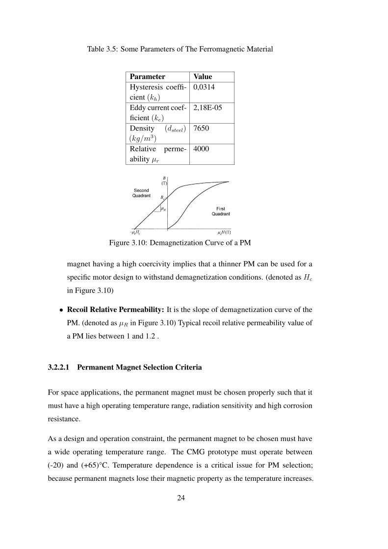
Table 3.5: Some Parameters of The Ferromagnetic Material

Parameter ValueHysteresis coeffi-cient (kh)

0,0314

Eddy current coef-ficient (ke)

2,18E-05

Density (dsteel)

(kg/m3)

7650

Relative perme-ability µr

4000

Figure 3.10: Demagnetization Curve of a PM

magnet having a high coercivity implies that a thinner PM can be used for a

specific motor design to withstand demagnetization conditions. (denoted as Hc

in Figure 3.10)

• Recoil Relative Permeability: It is the slope of demagnetization curve of the

PM. (denoted as µR in Figure 3.10) Typical recoil relative permeability value of

a PM lies between 1 and 1.2 .

3.2.2.1 Permanent Magnet Selection Criteria

For space applications, the permanent magnet must be chosen properly such that it

must have a high operating temperature range, radiation sensitivity and high corrosion

resistance.

As a design and operation constraint, the permanent magnet to be chosen must have

a wide operating temperature range. The CMG prototype must operate between

(-20) and (+65)°C. Temperature dependence is a critical issue for PM selection;

because permanent magnets lose their magnetic property as the temperature increases.

24

Remanent flux value Br of Samarium-Cobalt(Sa-Co) magnets is affected less than that

of Neodymium-Boron(Ne-B) equivalents. In addition, Curie temperature of PM’s is

essential in selecting a PM. Curie temperature is defined as the maximum temperature

value at which a PM loses its whole magnetic properties, that is no remanent flux

or coercive field intensity value is measured from the PM. For Samarium-Cobalt

permanent magnets, Curie temperature value is around 800 °C, while Neodymium-

Boron PM’s lie around 330°C. Considering the temperature conditions of the CMG,

both values are acceptable. As the final temperature constraint, maximum service

temperature is a parameter that must be taken into account. Service temperature is

the temperature value at which the thermal property of the magnet degrades such that

the magnetic properties cannot be reversed even the ambient or operating temperature

decreases. Maximum service temperature of Ne-B permanent magnets are around

110°C, while Sa-Co equivalents are around 330°C. A temperature value of 110°C can

be observed in a CMG, so selection of Ne-B permanent magnet may be risky.

As stated above, Sa-Co magnets have a better thermal characteristics. Another aspect

that must be pointed out is that these permanent magnets are highly resistant to

corrosion. Ne-B equivalents, on the other hand, appear to be more sensitive to the

corrosion issues. In order to decrease these effects, Ne-B permanent magnets can be

coated with an additional material. Yet, certain precautions must be taken for using

a Ne-B permanent magnet. To sum up, Sa-Co based permanent magnets such as

VACOMAX 225 HR have considerable thermal properties like thermal conductivity,

which makes these materials easy to remove heat on itself.

Additionally, radiation resistance is another issue that must be taken into consideration.

Radiation effects are highly dependent on the orbit, as well as the thickness of the

material used as a shield; but these effects are hardly known; but what is known is

that Sa-Co-based permanent magnets show an insensitive behaviour against radiation

whereas Ne-B equivalents degrade in performance depending on the radiation level.

Under these circumstances, due to the fact that Sa-Co permanent magnets have con-

siderably less temperature dependence, higher service and Curie temperature, better

thermal conductivity and less radiation sensitivity over Ne-B equivalents. VACOMAX

225 HR (Sm2Co17 Br at 1.03-1.1 T, Hr at 720-830 A/m) is chosen as the PM material

25

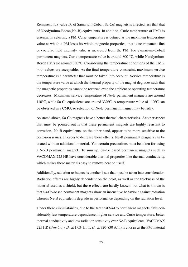
for the design process. Properties of the selected permanent magnet is given in Table

3.6, as the manufacturer data. As stated in core material selection, the permanent

magnet is assumed to be the same as the one used in previous CMG wheel motor

design conducted in [7].

Table 3.6: Properties of Selected PM [2]

Property ValueBr (T ) 1,03 - 1,1Hc (kA/m) 720 - 820µr 1,06 - 1,34Temperature coefficient -0,03Tcurie (C) 800Tservice (C) 350Thermal conductivity (W/(m. C)) 12

3.3 Magnetic Circuit

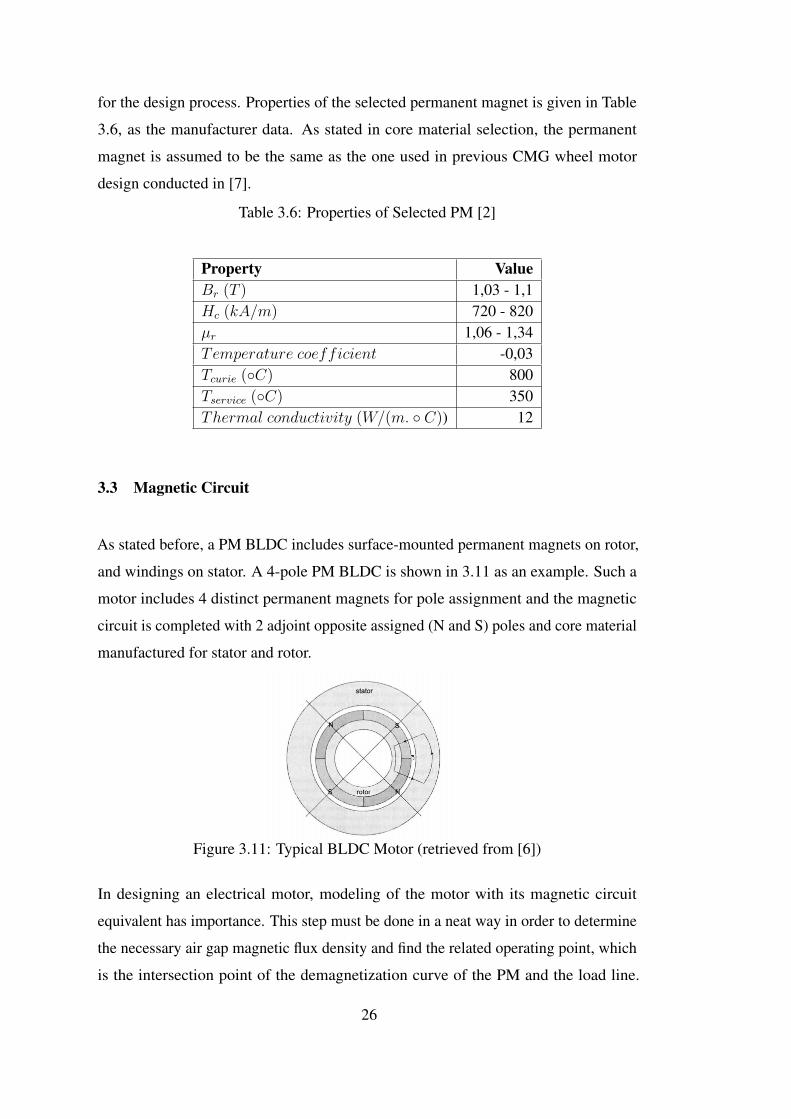
As stated before, a PM BLDC includes surface-mounted permanent magnets on rotor,

and windings on stator. A 4-pole PM BLDC is shown in 3.11 as an example. Such a

motor includes 4 distinct permanent magnets for pole assignment and the magnetic

circuit is completed with 2 adjoint opposite assigned (N and S) poles and core material

manufactured for stator and rotor.

Figure 3.11: Typical BLDC Motor (retrieved from [6])

In designing an electrical motor, modeling of the motor with its magnetic circuit

equivalent has importance. This step must be done in a neat way in order to determine

the necessary air gap magnetic flux density and find the related operating point, which

is the intersection point of the demagnetization curve of the PM and the load line.

26

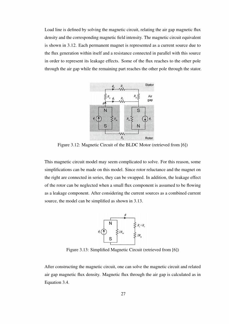
Load line is defined by solving the magnetic circuit, relating the air gap magnetic flux

density and the corresponding magnetic field intensity. The magnetic circuit equivalent

is shown in 3.12. Each permanent magnet is represented as a current source due to

the flux generation within itself and a resistance connected in parallel with this source

in order to represent its leakage effects. Some of the flux reaches to the other pole

through the air gap while the remaining part reaches the other pole through the stator.

Figure 3.12: Magnetic Circuit of the BLDC Motor (retrieved from [6])

This magnetic circuit model may seem complicated to solve. For this reason, some

simplifications can be made on this model. Since rotor reluctance and the magnet on

the right are connected in series, they can be swapped. In addition, the leakage effect

of the rotor can be neglected when a small flux component is assumed to be flowing

as a leakage component. After considering the current sources as a combined current

source, the model can be simplified as shown in 3.13.

Figure 3.13: Simplified Magnetic Circuit (retrieved from [6])

After constructing the magnetic circuit, one can solve the magnetic circuit and related

air gap magnetic flux density. Magnetic flux through the air gap is calculated as in

Equation 3.4.

27

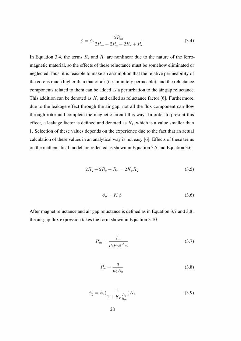
φ = φr2Rm

2Rm + 2Rg + 2Rs +Rr

(3.4)

In Equation 3.4, the terms Rs and Rr are nonlinear due to the nature of the ferro-

magnetic material, so the effects of these reluctance must be somehow eliminated or

neglected.Thus, it is feasible to make an assumption that the relative permeability of

the core is much higher than that of air (i.e. infinitely permeable), and the reluctance

components related to them can be added as a perturbation to the air gap reluctance.

This addition can be denoted as Kr and called as reluctance factor [6]. Furthermore,

due to the leakage effect through the air gap, not all the flux component can flow

through rotor and complete the magnetic circuit this way. In order to present this

effect, a leakage factor is defined and denoted as Kl, which is a value smaller than

1. Selection of these values depends on the experience due to the fact that an actual

calculation of these values in an analytical way is not easy [6]. Effects of these terms

on the mathematical model are reflected as shown in Equation 3.5 and Equation 3.6.

2Rg + 2Rs +Rr = 2KrRg (3.5)

φg = Klφ (3.6)

After magnet reluctance and air gap reluctance is defined as in Equation 3.7 and 3.8 ,

the air gap flux expression takes the form shown in Equation 3.10

Rm =lm

µoµrelAm(3.7)

Rg =g

µ0Ag(3.8)

φg = φr(1

1 +KrRgRm

)Kl (3.9)

28

φg = φrKl

1 +KrµrelgAmlmAg

(3.10)

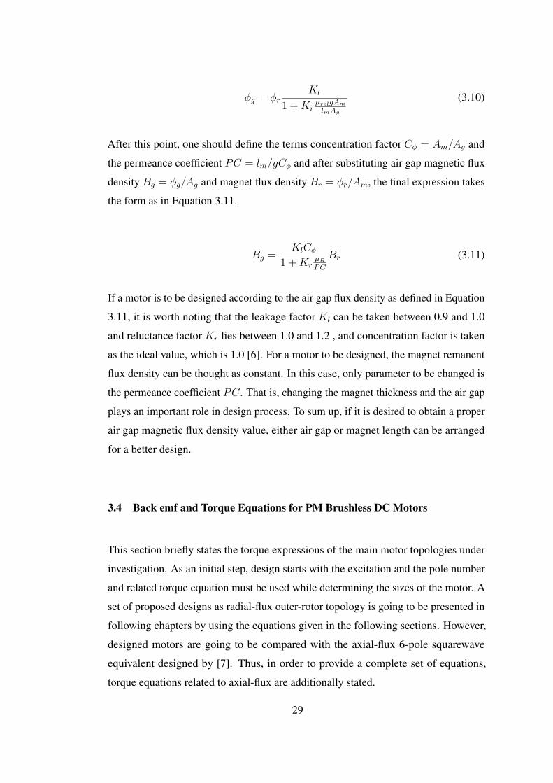
After this point, one should define the terms concentration factor Cφ = Am/Ag and

the permeance coefficient PC = lm/gCφ and after substituting air gap magnetic flux

density Bg = φg/Ag and magnet flux density Br = φr/Am, the final expression takes

the form as in Equation 3.11.

Bg =KlCφ

1 +KrµRPC

Br (3.11)

If a motor is to be designed according to the air gap flux density as defined in Equation

3.11, it is worth noting that the leakage factor Kl can be taken between 0.9 and 1.0

and reluctance factor Kr lies between 1.0 and 1.2 , and concentration factor is taken

as the ideal value, which is 1.0 [6]. For a motor to be designed, the magnet remanent

flux density can be thought as constant. In this case, only parameter to be changed is

the permeance coefficient PC. That is, changing the magnet thickness and the air gap

plays an important role in design process. To sum up, if it is desired to obtain a proper

air gap magnetic flux density value, either air gap or magnet length can be arranged

for a better design.

3.4 Back emf and Torque Equations for PM Brushless DC Motors

This section briefly states the torque expressions of the main motor topologies under

investigation. As an initial step, design starts with the excitation and the pole number

and related torque equation must be used while determining the sizes of the motor. A

set of proposed designs as radial-flux outer-rotor topology is going to be presented in

following chapters by using the equations given in the following sections. However,

designed motors are going to be compared with the axial-flux 6-pole squarewave

equivalent designed by [7]. Thus, in order to provide a complete set of equations,

torque equations related to axial-flux are additionally stated.

29

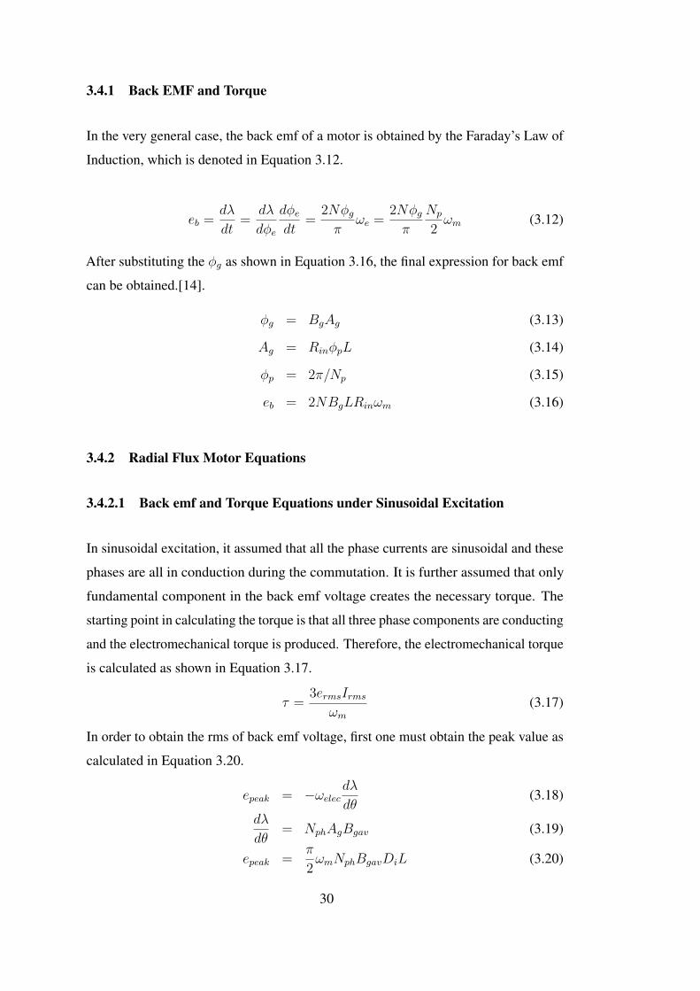
3.4.1 Back EMF and Torque

In the very general case, the back emf of a motor is obtained by the Faraday’s Law of

Induction, which is denoted in Equation 3.12.

eb =dλ

dt=

dλ

dφe

dφedt

=2Nφgπ

ωe =2Nφgπ

Np

2ωm (3.12)

After substituting the φg as shown in Equation 3.16, the final expression for back emf

can be obtained.[14].

φg = BgAg (3.13)

Ag = RinφpL (3.14)

φp = 2π/Np (3.15)

eb = 2NBgLRinωm (3.16)

3.4.2 Radial Flux Motor Equations

3.4.2.1 Back emf and Torque Equations under Sinusoidal Excitation

In sinusoidal excitation, it assumed that all the phase currents are sinusoidal and these

phases are all in conduction during the commutation. It is further assumed that only

fundamental component in the back emf voltage creates the necessary torque. The

starting point in calculating the torque is that all three phase components are conducting

and the electromechanical torque is produced. Therefore, the electromechanical torque

is calculated as shown in Equation 3.17.

τ =3ermsIrms

ωm(3.17)

In order to obtain the rms of back emf voltage, first one must obtain the peak value as

calculated in Equation 3.20.

epeak = −ωelecdλ

dθ(3.18)

dλ

dθ= NphAgBgav (3.19)

epeak =π

2ωmNphBgavDiL (3.20)

30

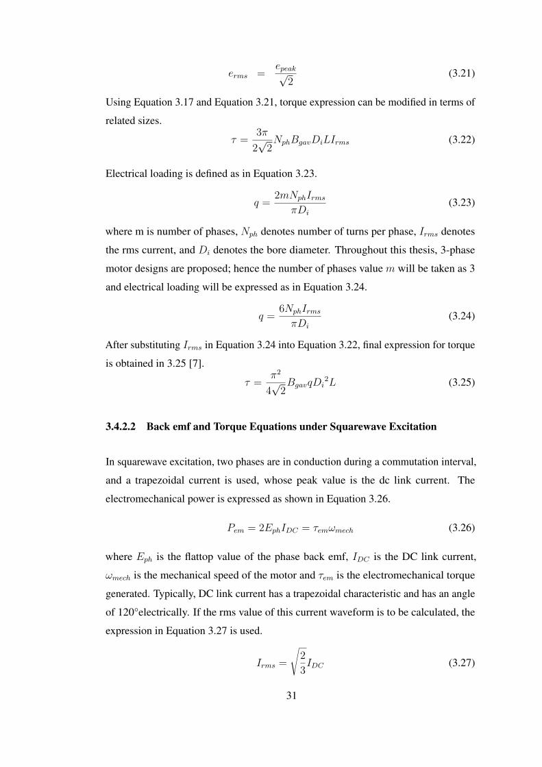
erms =epeak√

2(3.21)

Using Equation 3.17 and Equation 3.21, torque expression can be modified in terms of

related sizes.

τ =3π

2√

2NphBgavDiLIrms (3.22)

Electrical loading is defined as in Equation 3.23.

q =2mNphIrms

πDi

(3.23)

where m is number of phases, Nph denotes number of turns per phase, Irms denotes

the rms current, and Di denotes the bore diameter. Throughout this thesis, 3-phase

motor designs are proposed; hence the number of phases value m will be taken as 3

and electrical loading will be expressed as in Equation 3.24.

q =6NphIrmsπDi

(3.24)

After substituting Irms in Equation 3.24 into Equation 3.22, final expression for torque

is obtained in 3.25 [7].

τ =π2

4√

2BgavqDi

2L (3.25)

3.4.2.2 Back emf and Torque Equations under Squarewave Excitation

In squarewave excitation, two phases are in conduction during a commutation interval,

and a trapezoidal current is used, whose peak value is the dc link current. The

electromechanical power is expressed as shown in Equation 3.26.

Pem = 2EphIDC = τemωmech (3.26)

where Eph is the flattop value of the phase back emf, IDC is the DC link current,

ωmech is the mechanical speed of the motor and τem is the electromechanical torque

generated. Typically, DC link current has a trapezoidal characteristic and has an angle

of 120°electrically. If the rms value of this current waveform is to be calculated, the

expression in Equation 3.27 is used.

Irms =

√2

3IDC (3.27)

31

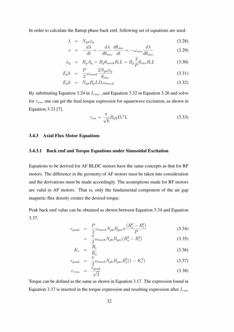
In order to calculate the flattop phase back emf, following set of equations are used.

λ = Nphφg (3.28)

e = −dλdt

= − dλ

dθelec

dθelecdt

= −ωelecdλ

dθelec(3.29)

φg = BgAg = BgθmechRiL = Bg2

PθelecRiL (3.30)

Eph =P

2ωmech

2Nphφgθelec

(3.31)

Eph = NphBgLDiωmech (3.32)

By substituting Equation 3.24 in Irms , and Equation 3.32 in Equation 3.26 and solve

for τem, one can get the final torque expression for squarewave excitation, as shown in

Equation 3.33 [7].

τem =π√6BgqDi

2L (3.33)

3.4.3 Axial Flux Motor Equations

3.4.3.1 Back emf and Torque Equations under Sinusoidal Excitation

Equations to be derived for AF BLDC motors have the same concepts as that for RF

motors. The difference in the geometry of AF motors must be taken into consideration

and the derivations must be made accordingly. The assumptions made for RF motors

are valid in AF motors. That is, only the fundamental component of the air gap

magnetic flux density creates the desired torque.

Peak back emf value can be obtained as shown between Equation 3.34 and Equation

3.37.

epeak =P

2ωmechNphBgavπ

(R2o −R2

i )

P(3.34)

=π

2ωmechNphBgav(R

2o −R2

i ) (3.35)

Kr =Ri

Ro

(3.36)

epeak =π

2ωmechNphBgavR

2o(1−K2

r ) (3.37)

erms =epeak√

2(3.38)

Torque can be defined as the same as shown in Equation 3.17. The expression found in

Equation 3.37 is inserted in the torque expression and resulting expression after Irms

32

is replaced with Equation 3.24 is given in Equation 3.40.

τem =3π

2√

2NphBgavR

2o(1−K2

r )Irms (3.39)

=π2

√2BgavqR

3oKr(1−K2

r ) (3.40)

3.4.3.2 Back emf and Torque Equations under Squarewave Excitation

While calculating the torque expression related to the squarewave excitation of the AF

motors, the initial point will also be the same as the derived expressions for RF motors.

Electromechanical power produced by such motors is expressed as stated in Equation

3.26.

The flux at air gap in AF motors is stated as in Equation 3.41.

φg = BgAg = Bgπ(R2

o −R2i )θmech

Pπ(3.41)

Eph, in addition, can be expressed as shown in Equation 3.45.

λ = Nphφg (3.42)

Eph = −dλdt

= − dλ

dθelec

dθelecdt

(3.43)

=P

2

2Nph

θmech

θmech(R2o −R2

i )

PωmechBg (3.44)

= NphBgR2o(1−K2

r )ωmech (3.45)

Kr =Ri

Ro

(3.46)

After substituting Eph found in Equation 3.45, one can obtain the torque expression as

shown in Equation 3.47.

τem = 2NphBgR2o(1−K2

r )IDC (3.47)

Substitution of IDC with it rms equivalent in Equation 3.47 and modifying the expres-

sion for electrical loading q yields the form given in Equation 3.48 .

τem =2√

2π√3BgqiR

3oKr(1−K2

r ) (3.48)

33

3.5 Literature Survey

In literature, there are several findings and results on the area of CMG designs and the

motor topologies related to CMG applications.

Radial flux motors can be used when relatively long shafts are to be included. As the

pole number increases, the torque capability of the motor increases but after a certain

increase, the increase in pole number leads to a decrease in torque capability; because

core losses inside the motor tend to increase. Furthermore, for an AF motor, making a

design with a small axial length, these motors are capable of delivering more torque

[15].

In [16], it is stated that an axial-flux topology has advantages on CMG applications

compared to the radial-flux topologies. Furthermore, increase in the pole number and

repeating the motor design process reduces the motor volume dramatically, which is

also discussed by [17], stating that single-sided axial-flux machines have a volumetric

advantage when compared to the radial-flux equivalents. [18] discusses the advantages

between RF topology and AF topology. According to [18], RF topologies show a

slightly better torque performance than AF topology, under the circumstances that

Di/L ratio does not exceed the value of 5. [12] gives a comprehensive information

about design guidelines, control strategies, cooling methods, PM selection and presents

the engineering tools used in a typical electrical motor design process as a FEA solution.

In [19], basic derivations are done for motors under different application types. These

include the maximum torque and acceleration limits, and acceleration capability is

presented for different applications. Reducing cogging torque effects in a permanent

magnet motor is well stated in [20], by explaining the effects of skewing, applying a

pole arc and defining notches in the stator teeth.

In general, there are not many papers on CMG design. Some patents such as [3]

explains the general working principles of the Control Moment Gyroscopes and states

that the main electrical motor used in such systems are brushless DC electrical motors.

In addition, [9] presents a comprehensive study on attitude control systems based

on Control Moment Gyroscopes. Here, [9] explains the working principles of these

systems clearly. Similar observations are made by [21] by explaining the Control

34

Moment Gyroscope types and the configurations in a typical satellite system.

In the next chapter, the design procedure of an outer-rotor brushless DC motor is

going to be stated, and necessary equations for sizing and performance are going to be

provided.

35

36

CHAPTER 4

DESIGN PROCEDURE OF OUTER-ROTOR BRUSHLESS DC

MOTOR TOPOLOGIES

This chapter describes the design procedure for proposed brushless DC motor topology.

First, equations are derived for RF motor topology under sinusoidal excitation case,

both for 2-pole topology and 6-pole topology. Then, the same procedure is summarized

for squarewave excitation, again for both 2-pole and 6-pole topologies.(see Figure 4.1)

Figure 4.1: Division of The Topologies

4.1 Introduction to the Design of an Outer-Rotor Permanent Magnet Brushless

DC Motor Configuration

The structure of an outer-rotor BLDC PM motor is given in Figure 4.2. In an outer-

rotor configuration, the locations of stator and rotor are made inside out. That is, the

stator of the motor is placed inside the rotor, and the rotor is placed outer side of the

motor. Main advantage of such system is that no slip ring is required while achieving

the electromechanical energy conversion, which is the same as a typical PM brushless

37

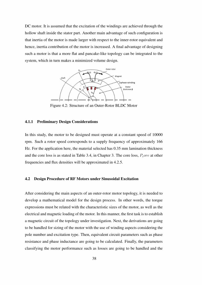
DC motor. It is assumed that the excitation of the windings are achieved through the

hollow shaft inside the stator part. Another main advantage of such configuration is

that inertia of the motor is made larger with respect to the inner-rotor equivalent and

hence, inertia contribution of the motor is increased. A final advantage of designing

such a motor is that a more flat and pancake-like topology can be integrated to the

system, which in turn makes a minimized volume design.

Figure 4.2: Structure of an Outer-Rotor BLDC Motor

4.1.1 Preliminary Design Considerations

In this study, the motor to be designed must operate at a constant speed of 10000

rpm. Such a rotor speed corresponds to a supply frequency of approximately 166

Hz. For the application here, the material selected has 0.35 mm lamination thickness

and the core loss is as stated in Table 3.4, in Chapter 3. The core loss, Pcore at other

frequencies and flux densities will be approximated in 4.2.5.

4.2 Design Procedure of RF Motors under Sinusoidal Excitation

After considering the main aspects of an outer-rotor motor topology, it is needed to

develop a mathematical model for the design process. In other words, the torque

expressions must be related with the characteristic sizes of the motor, as well as the

electrical and magnetic loading of the motor. In this manner, the first task is to establish

a magnetic circuit of the topology under investigation. Next, the derivations are going

to be handled for sizing of the motor with the use of winding aspects considering the

pole number and excitation type. Then, equivalent circuit parameters such as phase

resistance and phase inductance are going to be calculated. Finally, the parameters

classifying the motor performance such as losses are going to be handled and the

38

motor volume and mass is approximated. In this manner, the calculations are handled

according to the pole number and the excitation types, respectively. In this context,

the sinusoidal excitation case is investigated in this section, for both 2-pole and 6-pole

topologies. Afterwards, the squarewave excitation case is going to be discussed, again

for both 2-pole and 6-pole topologies.

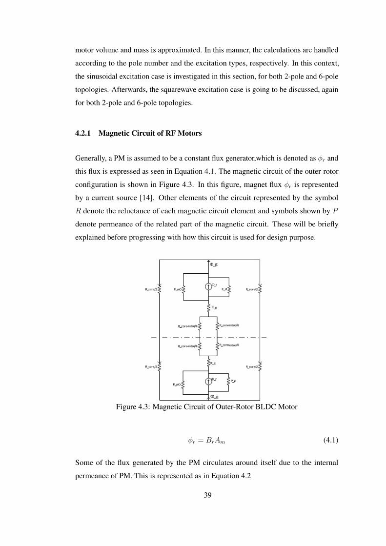
4.2.1 Magnetic Circuit of RF Motors

Generally, a PM is assumed to be a constant flux generator,which is denoted as φr and

this flux is expressed as seen in Equation 4.1. The magnetic circuit of the outer-rotor

configuration is shown in Figure 4.3. In this figure, magnet flux φr is represented

by a current source [14]. Other elements of the circuit represented by the symbol

R denote the reluctance of each magnetic circuit element and symbols shown by P

denote permeance of the related part of the magnetic circuit. These will be briefly

explained before progressing with how this circuit is used for design purpose.

Figure 4.3: Magnetic Circuit of Outer-Rotor BLDC Motor

φr = BrAm (4.1)

Some of the flux generated by the PM circulates around itself due to the internal

permeance of PM. This is represented as in Equation 4.2

39

Pm0 =µ0µrecAm

lm(4.2)

where µ0 is the permeability of vacuum, µrec is the relative permeability of the PM,

Am is the magnet area and lm is the magnet length. Magnet area is considered as

120°of magnet span and calculated according to the length at the middle, which indeed

gives a mean length when a 2-pole motor is considered. Furthermore, magnet area is

calculated as in Equation 4.3.

Am = α(Ri + g + lm/2)L (4.3)

In Equation 4.3, Ri denotes the stator radius, g denotes the air gap, L denotes the axial

length, and α denotes arc angle of the PM in radians. That is, if the magnet arc angle is

to be taken as 120°, then the term α becomes 23π. By adding the rotor leakage effects,

denoting as Prl and corresponding to a value of 10% of the internal permeance of the

internal permeance [14], the total permeance of the magnet is calculated in Equation

4.4. Additionally, the reluctance of the air gap is calculated as shown in Equation 4.5.

Pm = Pm0 + Prl = Pm0 + 0.1Pm0 = 1.1Pm0 (4.4)

Rg =g′

µ0Ag(4.5)

where g′ is the equivalent air gap calculated with the expression g′ = Kcg in which Kc

denotes the Carter’s Coefficient, and Ag is the area of the air gap. Carter’s Coefficient

must be taken into consideration in cases where slotting affects the mean air gap. In

this study, Carter’s Coefficient can be assumed to be as 1.05 [14]. Except from the air

gap, the reluctance of the air gap is dependent on the area of the air gap area and this

area is calculated as shown in Equation 4.6, following the same idea as the calculation

of magnet area.

Ag = (α(Ri + g/2) + 2g)(L+ 2g) (4.6)

The reluctance of the flux path in the stator core is calculated from Equation 4.7. In

40

Equation 4.7, µcore is the permeability of the flux path and lcore is the length of the

flux path (uniform flux distribution path is assumed) and calculated as in Equation 4.8.

Furthermore, area of the core is calculated as shown in Equation 4.9.

Rcore =lcore

µcoreAcore(4.7)

lcore =π(Di +Do)

2p(4.8)

Acore =L

2(Do −Di) (4.9)

where Do is the outer diameter of the core. In Equation 4.6, the core length is extended

by a “2g” term in order to take into account the fringing flux at the ends of the core

and give a proper margin. The air gap flux is assumed to cross the air gap only through

the magnets and is calculated from 4.10.

φg =φr

1 + Pm(Rg + Rcore4

)(4.10)

It must be noted that, this flux can also be written in terms of average air gap flux

density as in Equation 4.11.

BgAg =BrAm

1 + Pm(Rg + Rcore4

)(4.11)

The operating point of the magnet can be determined from the equivalent circuit, and

is found to be given by 4.12

Bm =1 + Prl(Rg + Rcore

4)

1 + Pm(Rg + Rcore4

)Br (4.12)

Now, the magnet flux density at the operating point Bm is determined for a given

geometry, using the slope of the B-H curve, magnetizing force Hm can be calculated

using Equation 4.13.

41

−Hm =Br −Bm

µ0µrec(4.13)

After substituting Br in 4.12 into 4.13, load line characteristics for the magnet can be

found as in Equation 4.14.

Bm = µ0µrecHm(1 + Prl(Rg + Rcore

4)

Pm0Rg

) (4.14)

The equations above describe how to establish the magnetic equivalent circuit of an

outer-rotor RF PM motor; given its dimensions and the properties of the core material

and the magnet. Once Bm, the operating point of the magnet is known, the flux

densities of various parts of the motor magnetic circuit can be found.

4.2.2 Determination of Motor Dimensions for Sinusoidal Excitation

In the design process, the torque requirement and the torque expression related to the

certain excitation the is the main starting point. Previously, it was stated that the torque

produced by the motor (τp) can be found from Equation 4.15 in case the BLDC motor

is excited from a sinusoidal voltage source.[22].

τp =π2

4√

2BgavqDi

2L (4.15)

In Equation 4.15, Bgav is the average flux density in the air gap, q is the electrical

loading, Di is the inner diameter and L is the axial length of the motor. Bgav and q

terms are given in Equations 4.16 and 4.17, respectively.

Bgav =φpoleApole

(4.16)

q =6NphIrmsπDi

(4.17)

where φpole denotes the flux at each pole and Apole denotes the pole area in Equation

4.16. In Equation 4.17, Nph denotes the number of turns per phase and Irms denotes

42

the rms current. Electrical loading basically clarifies total magnetomotive force per

unit length. Hence, number of turns per phase value must be first multiplied by 3 for

total number of turns, and total number of turns value must be multiplied by 2 for total

number of conductors within the motor. That is why the term 6 appears in Equation

4.17.

Bgav is a measure of saturation of the magnetic circuit and depends on the material

used as the core. This parameter is also related to core loss. q, on the other hand, is

related to copper loss and therefore is limited by the type of cooling. Previous study

conducted in [7] indicates that the current loading up to 6000 A/m can be handled

by the motor while the motor is accelerating with current density of J=7 A/mm2 in

the conductors. Once the motor reaches its steady-state speed, it is found that current

density falls down to 3 A/mm2 and the motor temperature remains within acceptable

limits.

One of the purposes of the investigation here is to compare the performance of the

two-rotor axial-flux PM motor designed in [7] with the outer-rotor radial-flux PM

motor. Because of this reason, both motors are designed with the same core material.

As in the axial flux motor design in [7], the value of the average air gap flux density is

limited to 0.43 T. The maximum flux density in any part of the motor is kept below

1.4 T, so that the material magnetic characteristics remain in its linear region and the

core loss is low.

At this point, the main aim here is to minimize the volume and the mass of the motor

with higher inertia and efficiency and to determine the main dimensions of the motor,

so that the motor is capable of producing the desired torque both in transient and

steady-state, satisfying the following requirements:

• Average air gap magnetic flux density Bgav must be 0.43 T, which is taken as

the same that in [7].

• JCu = 7 A/mm2 and less than 3 A/mm2 at steady-state.

• Electrical loading q must be less than 6000 A-turn/m during starting and less

than 3000 A-turn/m at steady-state.

• Acceleration torque must be 50 mN-m maximum.

43

• Steady-state torque (at 10000 rpm) must be 32 mN-m. This value is set so

that the net torque becomes zero and motor continues to operate without any

acceleration.

• The flux density in other parts of the core must be 1.4 T maximum. The average

air gap magnetic flux density is taken as 0.43 T. This create a constraint that

the average magnetic flux density at the core material must become 2 times the

average air gap magnetic flux density, which is 0.86 T. The peak value of such

averaged flux density value is found simply by multiplying with π/2, which

makes 1.35 T. Hence, a core flux density of 1.4 T is an acceptable value due to

the fact the core material starts to saturate after 1.4 T.

The problem can be handled in a simple way by setting the average air gap magnetic

flux density Bgav as 0.43 T and the current density of the copper to its maximum value,

which is 7 A/mm2.

The problem is now determination of basic dimensions such as slot area Aslot, slot

depth hs, back core length hsbc, inner diameterDi, core length L and the outer-diameter

of the motor Do.

The slot width and the tooth width are assumed to be equal in order to reduce the

number of unknowns. Therefore, three parameters are left unknown, namely hs,Di and

L, where hs and hsbc are dependent variables. Therefore, we need three equations to

solve the required variables. However, there are two known constraints, which are the

current density JCu and the average air gap flux densityBgav. Therefore,RDL = Di/L

ratio is chosen as a parameter so that the number of unknowns is reduced to two.

In the calculations below the shaft diameter Dshaft is chosen as 5 mm and is kept

constant throughout the whole design process. The flux density behind the slots Bsbc

can be written as shown in Equation 4.19.

φpole = BgavApole (4.18)

φsbc = BsbcAsbc (4.19)

φsbc =φpole

2(4.20)

44

Apole =πDiL

p(4.21)

Asbc = hsbcL (4.22)

BgavπDiL

2p= BsbchbcL (4.23)

In addition, the back core depth hsbc is expressed as in Equation 4.24.

hsbc =Di − 2hs −Dshaft

2(4.24)

By substituting Equation 4.24 in Equation 4.18, one can solve the quadratic equation

and slot depth hs can be found as in Equation 4.25.

hs =1

2[Di(1−

Bgavπ

Bsbcp)−Dshaft] (4.25)

It must be noted that the flux density at back core Bsbc is a dependent variable, which

is a function of Di. In addition, electrical loading of a motor can also be expressed as

shown in Equation 4.26.

q =JCuKCuAslot

πDi

(4.26)

where JCu is the current density of the copper wire, KCu is the slot fill factor (taken

0.4 here) and Aslot is the total slot area. Aslot can be expressed as shown in Equation

4.27. It must be noted that, the total number of slots are taken as 18 throughout the

design process. Since 3-phase designs are going to be handled with 2-pole and 6-pole

topologies, the chosen slot number is acceptable.

Aslot =π

2[(Di

2)2 − (

Di

2− hs)2] (4.27)

After substituting the slot depth hs found in Equation 4.25 in Equation 4.27, and the

resulting expression in 4.26, the electrical loading expression also becomes a function

of Di, as shown in 4.28.

45

q =JCuKCu

2Di

[(Di

2)2 − (

Di

2− hs)2] (4.28)

The torque equation of the electrical motor under sinusoidal excitation was previously

stated as in the form in Equation 4.15. When it is written by substituting RDL and is

solved for electrical loading, the equation takes the following form, as in Equation

4.29.

q =τpRDL

π2

4√2BgavDi

3(4.29)

The electrical loading values expressed as in Equation 4.29 and Equation 4.28 are

both functions of Di. All other parameters in the expressions such as peak torque τp,

average air gap flux density Bgav, current density JCu, slot fill factor KCu are known,

and ratio RDL can be changed easily. Therefore, for a given value of RDL; Di can be

solved from Equation 4.29. In addition, hs can be calculated from Equation 4.25. It

must be noted that Do can be calculated from Equation 4.30.

Do = Di + 2g + 2lm + 2hsbc (4.30)

4.2.3 Winding Design

After sizing is handled, the winding design must be made, so that the current density

requirement is met and the resulting winding fits into the slots properly. While doing

this, one must make sure that the electrical loading limits are not exceeded. Once these

dimensions are found, it becomes possible to adjust the inertia to the desired value

(by increasing the rotating rotor frame thickness, namely the outer diameter Do) and

compare the resulting volume and mass of the new design with other designs.

After the main sizes are obtained, the next task is considering the windings. The

motor in this work is supplied from a DC bus whose minimum voltage level is 18V.

Therefore, the winding design is made so that, even at this DC bus level, the motor

meets the requirements. The peak value of the line-voltage level, at minimum DC

bus voltage is estimated to be 16 V, taking into account the semiconductor voltage

46

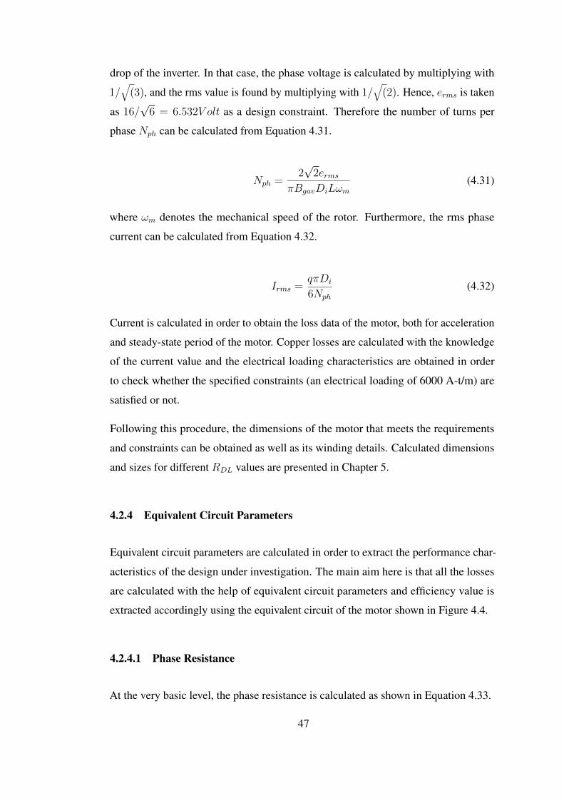
drop of the inverter. In that case, the phase voltage is calculated by multiplying with

1/√

(3), and the rms value is found by multiplying with 1/√

(2). Hence, erms is taken

as 16/√

6 = 6.532V olt as a design constraint. Therefore the number of turns per

phase Nph can be calculated from Equation 4.31.

Nph =2√

2ermsπBgavDiLωm

(4.31)

where ωm denotes the mechanical speed of the rotor. Furthermore, the rms phase

current can be calculated from Equation 4.32.

Irms =qπDi

6Nph

(4.32)

Current is calculated in order to obtain the loss data of the motor, both for acceleration

and steady-state period of the motor. Copper losses are calculated with the knowledge

of the current value and the electrical loading characteristics are obtained in order

to check whether the specified constraints (an electrical loading of 6000 A-t/m) are

satisfied or not.

Following this procedure, the dimensions of the motor that meets the requirements

and constraints can be obtained as well as its winding details. Calculated dimensions

and sizes for different RDL values are presented in Chapter 5.

4.2.4 Equivalent Circuit Parameters

Equivalent circuit parameters are calculated in order to extract the performance char-

acteristics of the design under investigation. The main aim here is that all the losses

are calculated with the help of equivalent circuit parameters and efficiency value is

extracted accordingly using the equivalent circuit of the motor shown in Figure 4.4.

4.2.4.1 Phase Resistance

At the very basic level, the phase resistance is calculated as shown in Equation 4.33.

47

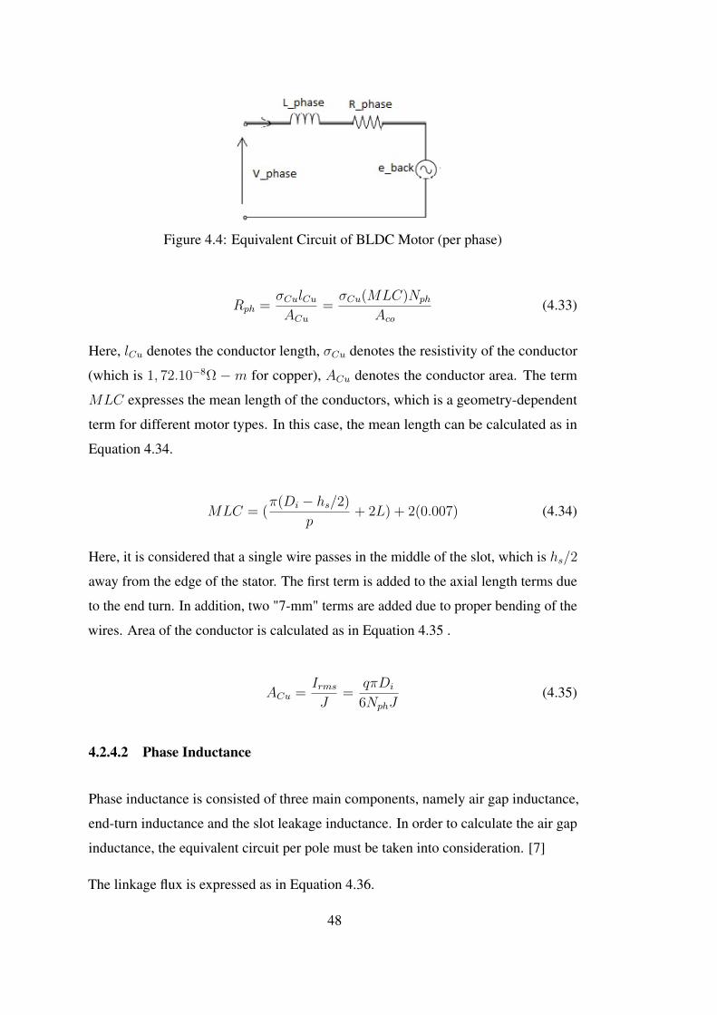
Figure 4.4: Equivalent Circuit of BLDC Motor (per phase)

Rph =σCulCuACu

=σCu(MLC)Nph

Aco(4.33)

Here, lCu denotes the conductor length, σCu denotes the resistivity of the conductor

(which is 1, 72.10−8Ω −m for copper), ACu denotes the conductor area. The term

MLC expresses the mean length of the conductors, which is a geometry-dependent

term for different motor types. In this case, the mean length can be calculated as in

Equation 4.34.

MLC = (π(Di − hs/2)

p+ 2L) + 2(0.007) (4.34)

Here, it is considered that a single wire passes in the middle of the slot, which is hs/2

away from the edge of the stator. The first term is added to the axial length terms due

to the end turn. In addition, two "7-mm" terms are added due to proper bending of the

wires. Area of the conductor is calculated as in Equation 4.35 .

ACu =IrmsJ

=qπDi

6NphJ(4.35)

4.2.4.2 Phase Inductance

Phase inductance is consisted of three main components, namely air gap inductance,

end-turn inductance and the slot leakage inductance. In order to calculate the air gap

inductance, the equivalent circuit per pole must be taken into consideration. [7]

The linkage flux is expressed as in Equation 4.36.

48

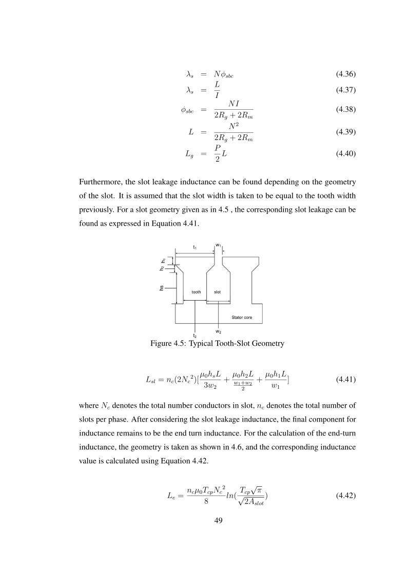
λs = Nφsbc (4.36)

λs =L

I(4.37)

φsbc =NI

2Rg + 2Rm

(4.38)

L =N2

2Rg + 2Rm

(4.39)

Lg =P

2L (4.40)

Furthermore, the slot leakage inductance can be found depending on the geometry

of the slot. It is assumed that the slot width is taken to be equal to the tooth width

previously. For a slot geometry given as in 4.5 , the corresponding slot leakage can be

found as expressed in Equation 4.41.

Figure 4.5: Typical Tooth-Slot Geometry

Lsl = nc(2Nc2)[µ0hsL

3w2

+µ0h2Lw1+w2

2

+µ0h1L

w1

] (4.41)

where Nc denotes the total number conductors in slot, nc denotes the total number of

slots per phase. After considering the slot leakage inductance, the final component for

inductance remains to be the end turn inductance. For the calculation of the end-turn

inductance, the geometry is taken as shown in 4.6, and the corresponding inductance

value is calculated using Equation 4.42.

Le =ncµ0TcpNc

2

8ln(

Tcp√π√

2Aslot) (4.42)

49

Figure 4.6: End Turn Geometry for Calculation of End-Turn Inductance

Aslot = w2hs +w1 + w2

2h2 + h1w1 (4.43)

4.2.5 Losses

Basically, the losses in an electromechanical environment are due to wiring and the

core material, as stated in Chapter 3. These losses are called as resistive losses and

core losses, respectively. Resistive losses represent the heat dissipation of the wires

due to their resistance, and the core losses represent the heat dissipation due to the

changing magnetic field in a core material. Core losses consist of hysteresis losses and

eddy current losses. These losses are expressed as in Equation 4.46 .

Ph = khfBn (4.44)

Pe = kef2B2 (4.45)

Pcore = Ph + Pe (4.46)

where kh is the hysteresis coefficient and ke is the eddy current coefficient, both of

which are material-dependent constant coefficients. Furthermore, f is the electrical

frequency, B is the peak magnetic flux density reached in the core. By using the

equations above, one can obtain the core loss Pcore in terms of Watts per unit mass

(Watts/kg) . Hence, this quantity must be multiplied with the total mass of the core

material in order to obtain the total core loss value. The term n is called Steinmetz

exponent and varies between 1.5 and 2.5, depending on the core material. For a typical

iron core, it can be taken as 1.6 . In this study, the Steinmetz exponent will be taken as

50

2 [23]. Core loss parameters are taken from Table 3.4, as stated in Chapter 3.

Resistive losses are calculated as shown from Equation 4.47 to Equation 4.50.

Pcopper = 3I2in−rmsRph (4.47)

Iin−rms = Irms +Pcore

3Vph−rms(4.48)

Vph−rms =√

(ZIrms)2 + e2rms (4.49)

Z =√

(ωLph)2 +R2ph (4.50)

where Pcopper denotes the resistive loss, Iin−rms denotes the input current in rms form,

Rph and Lph are the phase resistance and phase inductance, respectively, Irms is the

rms current, Pcore denotes the core losses, Vph−rms denotes the phase voltage in rms

form and Z denotes the total phase impedance.

4.2.6 Motor Mass, Volume, Inertia and Efficiency

While calculating the mass and the volume of the motor, the parts in which the

electromechanical energy conversion takes place are taken into consideration. That is,

all housing, bearing, winding and other terms are ignored for the ease of calculations.

In such a case, the mass of motor includes the mass of the stator, the mass of the rotor

and the mass of PM. Mass of the rotor is simply the mass of a cylinder with hollow

and the mass of the PM can be handled by multiplying the area with the axial length,

so calculation of these masses is quite easy. On the other hand, calculation of the mass

of the stator is relatively difficult due to the existence of slot geometry and teeth. Mass

of the rotor is expressed as in Equation 4.51.

Mrotor = π[(Do/2)2 − ((Do − 2hsbc)/2)2]Ldcore (4.51)

whereDo is the outer diameter, hsbc is the stator back core depth, which also determines

the thickness of the rotor shell, L is the axial length and dcore is the density of core

material. In addition, mass of the PM can be calculated as shown in Equation 4.52 .

51

Mmagnet =α

2(Di + 2g +

lm2

)lm2pLdmagnet (4.52)

where α is the arc angle of the magnet and dmagnet is the density of the magnet

material. All other parameters are previously calculated and known quantities. In

order to calculate the mass of the stator, it is plausible to divide this mass into sections.

That is, the stator is composed of two sections, one is a hollow cylinder and the other

is the group of teeth, number of which is equal to the number of slots. In this case,

calculation of the the mass of the stator is shown between Equations 4.53 and 4.56.

Mhollow = π(Dshaft + hsbc)hsbcLdcore (4.53)

Mteeth = SAtoothLdcore (4.54)

= ShswsLdcore (4.55)

Mstator = Mhollow +Mteeth (4.56)

Calculation of the volume of the motor is quite easy. In this case, only outer diameter

value Do and axial length L values are needed. Final expression is shown in Equation

4.57.

Vmotor = π(Ro)2L (4.57)

Additionally, inertia of the motor can be calculated as the inertia of the rotating part,

which is the rotor. Since the magnets are thinner as compared to the rotor, the effect of

magnet inertia is neglected. Calculation of the rotor inertia is simply calculation of a

cylindrical shell part, which can be calculated as shown in Equation

Jmotor =1

2Mrotor(R

2o + (Ro − hsbc)2) (4.58)

Finally, the efficiency of the motor, denoted as η can be calculated as in Equation

η =PoutPin

=Pout

Pout + Ptotal−loss=

PoutPout + Pcore + Pcopper

(4.59)

52

4.3 Design Procedure of RF Motors under Squarewave Excitation

As mentioned earlier, the design process of RF motors are divided into two major

sub-processes according to the excitation type and the sinusoidal case was covered.

Related expressions and other calculations are presented by considering the variations

in pole number, which can be thought as the minor processes for the design process.

In this section, the relations for squarewave excitation is presented. It must be noted

that the magnetic circuit derived for RF motor does not change for the excitation type,

the related section will not be covered again.

4.3.1 Determination of Motor Dimensions for Squarewave Excitation

The starting point of the design process in context of squarewave excitation is almost

similar to that of sinusoidal case. The torque expression as an initial point differs

from the one used in sinusoidal excitation. The torque τp produced by an RF motor, if

excited with a squarewave, is expressed in Equation 4.60.

τp =π√6BgqDi

2L (4.60)

In Equation 4.60, Bg is the flat top value of the flux density in the air gap, q is the

electrical loading, Di is the inner diameter and L is the axial length, all of which are

the same parameters for that of the sinusoidal excitation.

As stated previously,Bg is a measure of saturation of the magnetic circuit (and therefore

stated as magnetic loading in various sources) and depends on the material used for

the core. This parameter is also related to core loss. q, on the other hand, is related to

the copper loss and therefore is limited by the type of cooling. Experience from [7]

indicates that the current loading up to 6000 A-t/m can be handled by the motor while

the motor is accelerating with current density of J=7 A/mm2 in the conductors. Once

the motor reaches its steady-state speed, it is found that current density falls down to 3

A/mm2 and the motor temperature remains within acceptable limits.

At this point, the problem is determining the main dimensions of the motor, so that the

53

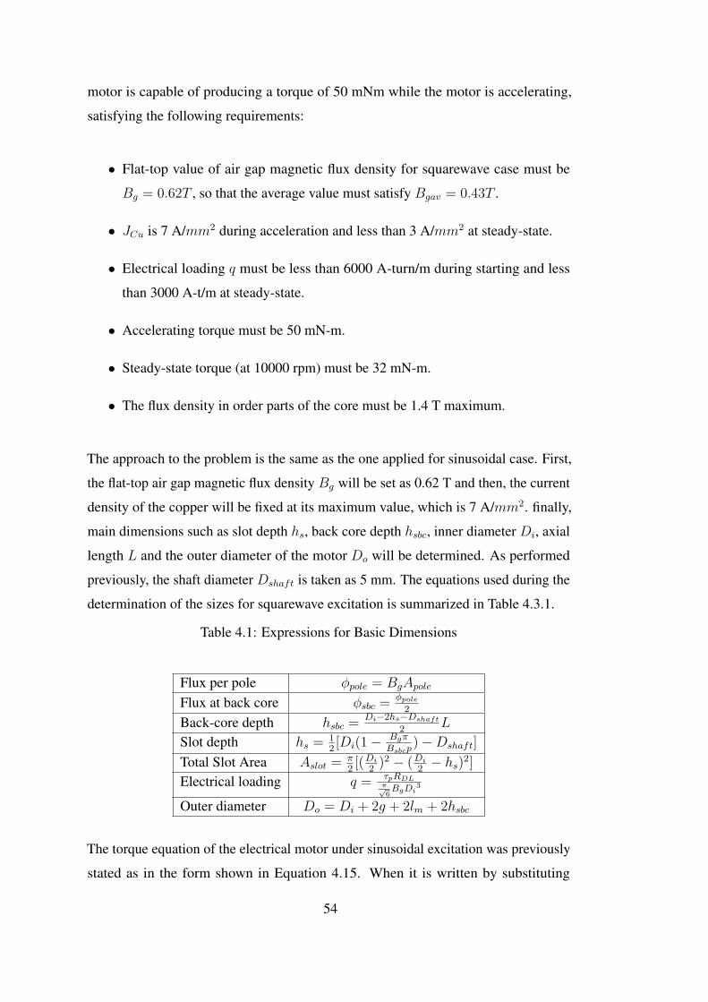
motor is capable of producing a torque of 50 mNm while the motor is accelerating,

satisfying the following requirements:

• Flat-top value of air gap magnetic flux density for squarewave case must be

Bg = 0.62T , so that the average value must satisfy Bgav = 0.43T .

• JCu is 7 A/mm2 during acceleration and less than 3 A/mm2 at steady-state.

• Electrical loading q must be less than 6000 A-turn/m during starting and less

than 3000 A-t/m at steady-state.

• Accelerating torque must be 50 mN-m.

• Steady-state torque (at 10000 rpm) must be 32 mN-m.

• The flux density in order parts of the core must be 1.4 T maximum.

The approach to the problem is the same as the one applied for sinusoidal case. First,

the flat-top air gap magnetic flux density Bg will be set as 0.62 T and then, the current

density of the copper will be fixed at its maximum value, which is 7 A/mm2. finally,

main dimensions such as slot depth hs, back core depth hsbc, inner diameter Di, axial

length L and the outer diameter of the motor Do will be determined. As performed

previously, the shaft diameter Dshaft is taken as 5 mm. The equations used during the

determination of the sizes for squarewave excitation is summarized in Table 4.3.1.

Table 4.1: Expressions for Basic Dimensions

Flux per pole φpole = BgApole

Flux at back core φsbc =φpole2

Back-core depth hsbc =Di−2hs−Dshaft

2L

Slot depth hs = 12[Di(1− Bgπ

Bsbcp)−Dshaft]

Total Slot Area Aslot = π2[(Di

2)2 − (Di

2− hs)2]

Electrical loading q = τpRDLπ√6BgDi

3

Outer diameter Do = Di + 2g + 2lm + 2hsbc

The torque equation of the electrical motor under sinusoidal excitation was previously

stated as in the form shown in Equation 4.15. When it is written by substituting

54

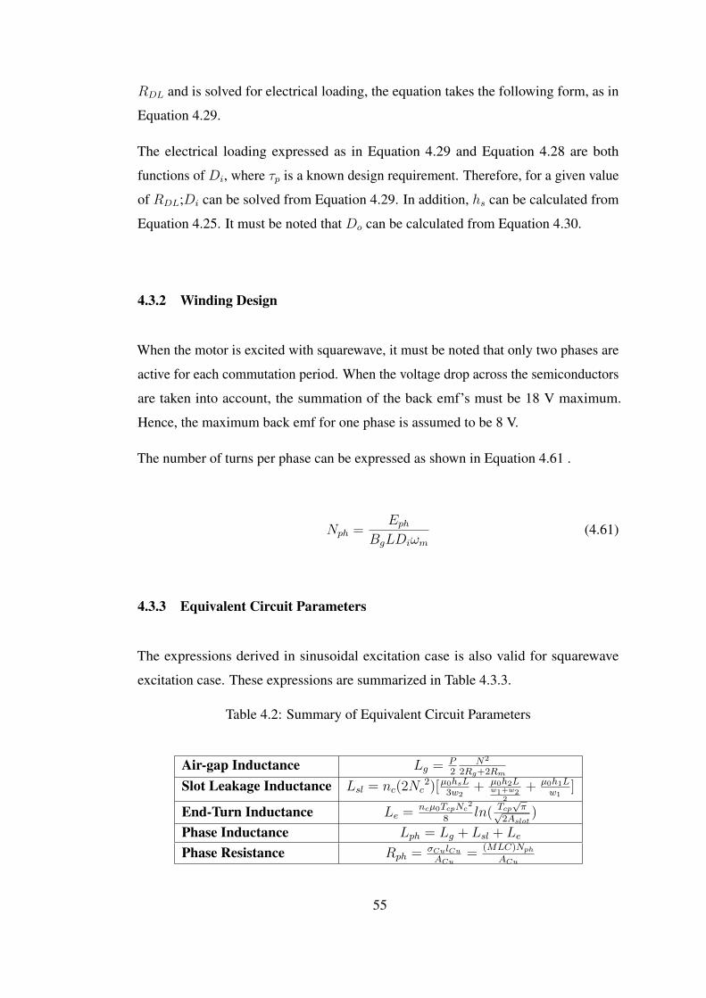
RDL and is solved for electrical loading, the equation takes the following form, as in

Equation 4.29.

The electrical loading expressed as in Equation 4.29 and Equation 4.28 are both

functions of Di, where τp is a known design requirement. Therefore, for a given value

of RDL;Di can be solved from Equation 4.29. In addition, hs can be calculated from

Equation 4.25. It must be noted that Do can be calculated from Equation 4.30.

4.3.2 Winding Design

When the motor is excited with squarewave, it must be noted that only two phases are

active for each commutation period. When the voltage drop across the semiconductors

are taken into account, the summation of the back emf’s must be 18 V maximum.

Hence, the maximum back emf for one phase is assumed to be 8 V.

The number of turns per phase can be expressed as shown in Equation 4.61 .

Nph =Eph

BgLDiωm(4.61)

4.3.3 Equivalent Circuit Parameters

The expressions derived in sinusoidal excitation case is also valid for squarewave

excitation case. These expressions are summarized in Table 4.3.3.

Table 4.2: Summary of Equivalent Circuit Parameters

Air-gap Inductance Lg = P2

N2

2Rg+2Rm

Slot Leakage Inductance Lsl = nc(2Nc2)[µ0hsL

3w2+ µ0h2L

w1+w22

+ µ0h1Lw1

]

End-Turn Inductance Le = ncµ0TcpNc2

8ln( Tcp

√π√

2Aslot)

Phase Inductance Lph = Lg + Lsl + Le

Phase Resistance Rph = σCulCuACu

=(MLC)Nph

ACu

55

4.3.4 Losses

In calculation of losses, the same procedure is applied as done for the sinusoidal

excitation. Here, the flat-top value for the magnetic air-gap flux density must be used.

While calculating the average flux density at tooth, fundamental component of the

air gap magnetic flux density is taken into account. The resulting peak flux density

at stator is compared with the maximum peak flux density value of the core and the

whether it is suitable or not is investigated. While calculating copper losses, DC

link current must be used due to the fact that two phases are excited in squarewave

excitation. The required equations are stated in Equations from 4.62 to 4.65.

Iin−rms = Irms +Pcore3VDC

√2

3(4.62)

VDC = 2IrmsRph + Eph (4.63)

IDC =

√3

2Iin−rms (4.64)

Pco = 2I2DCRph (4.65)

4.3.5 Motor Mass, Volume, Inertia and Efficiency

Motor volume, mass and inertia values are calculated in the way same as used in

sinusoidal case. The equations are summarized in Table 4.3.5.

Table 4.3: Summary of Motor Mass, Volume, Inertia and Efficiency Equations

Rotor Mass Mrotor = π[(Do/2)2 − ((Do − 2hsbc)/2)2]LdcoreMagnet Mass Mmagnet = α

2(Di + 2g + lm

2) lm

2pLdmagnet

Hollow Mass Mhollow = π(Dshaft + hsbc)hsbcLdcoreTeeth Mass Mteeth = ShswsLdcoreStator Mass Mstator = Mhollow +Mteeth

Volume Vmotor = πR2oL

Inertia Jmotor = 0.5Mrotor(R2o + (Ro − hsbc)2)

Efficiency η = PoutPin

56

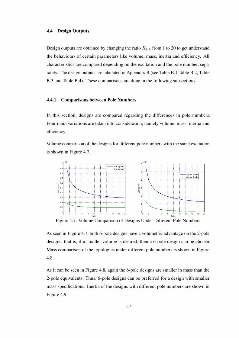
4.4 Design Outputs

Design outputs are obtained by changing the ratio RDL from 1 to 20 to get understand

the behaviours of certain parameters like volume, mass, inertia and efficiency. All

characteristics are compared depending on the excitation and the pole number, sepa-

rately. The design outputs are tabulated in Appendix B (see Table B.1,Table B.2, Table

B.3 and Table B.4). These comparisons are done in the following subsections.

4.4.1 Comparisons between Pole Numbers

In this section, designs are compared regarding the differences in pole numbers.

Four main variations are taken into consideration, namely volume, mass, inertia and

efficiency.

Volume comparison of the designs for different pole numbers with the same excitation

is shown in Figure 4.7.

Figure 4.7: Volume Comparison of Designs Under Different Pole Numbers

As seen in Figure 4.7, both 6-pole designs have a volumetric advantage on the 2-pole

designs, that is, if a smaller volume is desired, then a 6-pole design can be chosen.

Mass comparison of the topologies under different pole numbers is shown in Figure

4.8.

As it can be seen in Figure 4.8, again the 6-pole designs are smaller in mass than the

2-pole equivalents. Thus, 6-pole designs can be preferred for a design with smaller

mass specifications. Inertia of the designs with different pole numbers are shown in

Figure 4.9.

57

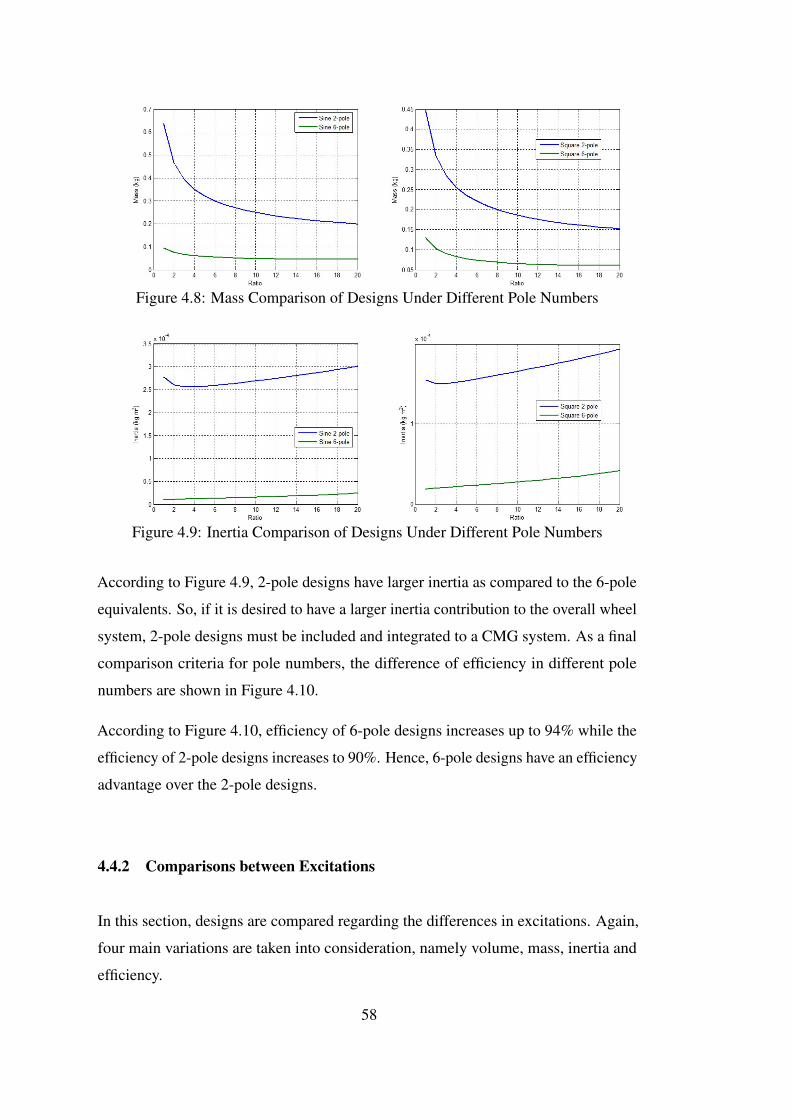
Figure 4.8: Mass Comparison of Designs Under Different Pole Numbers

Figure 4.9: Inertia Comparison of Designs Under Different Pole Numbers

According to Figure 4.9, 2-pole designs have larger inertia as compared to the 6-pole

equivalents. So, if it is desired to have a larger inertia contribution to the overall wheel

system, 2-pole designs must be included and integrated to a CMG system. As a final

comparison criteria for pole numbers, the difference of efficiency in different pole

numbers are shown in Figure 4.10.

According to Figure 4.10, efficiency of 6-pole designs increases up to 94% while the

efficiency of 2-pole designs increases to 90%. Hence, 6-pole designs have an efficiency

advantage over the 2-pole designs.

4.4.2 Comparisons between Excitations

In this section, designs are compared regarding the differences in excitations. Again,

four main variations are taken into consideration, namely volume, mass, inertia and

efficiency.

58

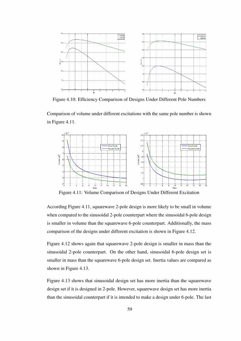
Figure 4.10: Efficiency Comparison of Designs Under Different Pole Numbers

Comparison of volume under different excitations with the same pole number is shown

in Figure 4.11.

Figure 4.11: Volume Comparison of Designs Under Different Excitation

According Figure 4.11, squarewave 2-pole design is more likely to be small in volume

when compared to the sinusoidal 2-pole counterpart where the sinusoidal 6-pole design

is smaller in volume than the squarewave 6-pole counterpart. Additionally, the mass

comparison of the designs under different excitation is shown in Figure 4.12.

Figure 4.12 shows again that squarewave 2-pole design is smaller in mass than the

sinusoidal 2-pole counterpart. On the other hand, sinusoidal 6-pole design set is

smaller in mass than the squarewave 6-pole design set. Inertia values are compared as

shown in Figure 4.13.

Figure 4.13 shows that sinusoidal design set has more inertia than the squarewave

design set if it is designed in 2-pole. However, squarewave design set has more inertia

than the sinusoidal counterpart if it is intended to make a design under 6-pole. The last

59

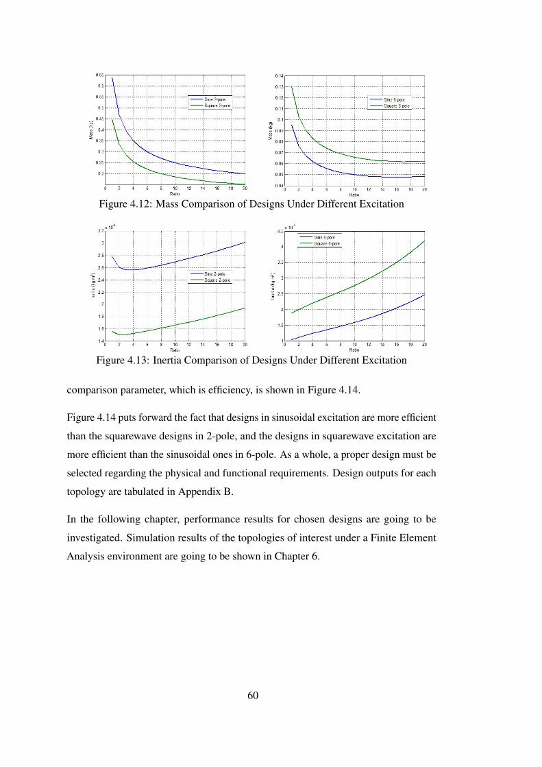
Figure 4.12: Mass Comparison of Designs Under Different Excitation

Figure 4.13: Inertia Comparison of Designs Under Different Excitation

comparison parameter, which is efficiency, is shown in Figure 4.14.

Figure 4.14 puts forward the fact that designs in sinusoidal excitation are more efficient

than the squarewave designs in 2-pole, and the designs in squarewave excitation are

more efficient than the sinusoidal ones in 6-pole. As a whole, a proper design must be

selected regarding the physical and functional requirements. Design outputs for each

topology are tabulated in Appendix B.

In the following chapter, performance results for chosen designs are going to be

investigated. Simulation results of the topologies of interest under a Finite Element

Analysis environment are going to be shown in Chapter 6.

60

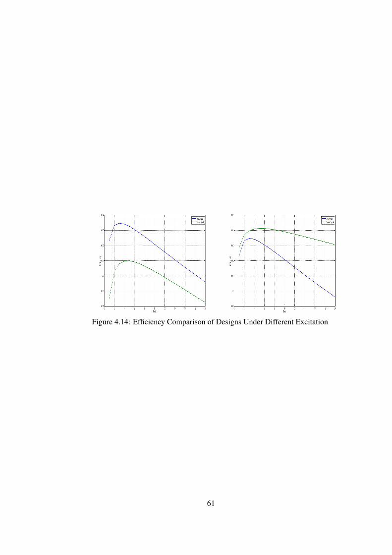
Figure 4.14: Efficiency Comparison of Designs Under Different Excitation

61

62

CHAPTER 5

ANALYTICAL RESULTS

This chapter includes the analytical results of the design procedure stated in Chapter

4. In order to determine the design outputs, MATLAB environment is used. In this

manner, script codes including sizing and performance equations are prepared for

each excitation and topology in separate m-files, and basic sizes, equivalent circuit

parameters and winding details, as well as some performance criteria such as losses,

efficiency, required current and back emf are calculated, as defined in Chapter 4. At

the end of the process, separate tables are prepared for each design by changing Di/L

ratio from 0.7 to 20 with irregular step sizes, and for a chosen ratio, related graphs

are presented. The point to be noted here is that the slot number in each proposed

design is taken to be 18, and full-pitched concentrated windings are assumed to be

used. Moreover, a coil extension is taken into account which has a value of 7 mm.

Parameter descriptions are given in Appendix A, and the dimensions related to slots

and teeth are defined based on Figure 5.1. Analytical results are presented in its related

section or subsection, with the motor torque profile shown in Figure 3.4.

5.1 Analytical Results

Analytical results are obtained by setting the electrical loading value as 6000 A.t/m,

motor torque as 50 mN-m while accelerating and 32 mN-m at rated speed, and phase

voltage as 16 Volts, as defined in Chapter 4. Furthermore, it is desired to have an

average air gap magnetic flux density value of 0.43 T. While conducting the design

procedure, it is guaranteed that the average air gap magnetic flux density value is

63

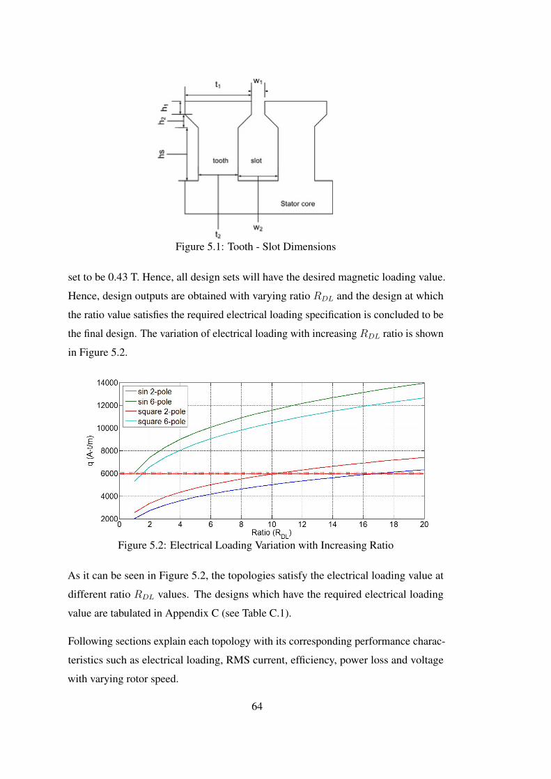
Figure 5.1: Tooth - Slot Dimensions

set to be 0.43 T. Hence, all design sets will have the desired magnetic loading value.

Hence, design outputs are obtained with varying ratio RDL and the design at which

the ratio value satisfies the required electrical loading specification is concluded to be

the final design. The variation of electrical loading with increasing RDL ratio is shown

in Figure 5.2.

Figure 5.2: Electrical Loading Variation with Increasing Ratio

As it can be seen in Figure 5.2, the topologies satisfy the electrical loading value at

different ratio RDL values. The designs which have the required electrical loading

value are tabulated in Appendix C (see Table C.1).

Following sections explain each topology with its corresponding performance charac-

teristics such as electrical loading, RMS current, efficiency, power loss and voltage

with varying rotor speed.

64

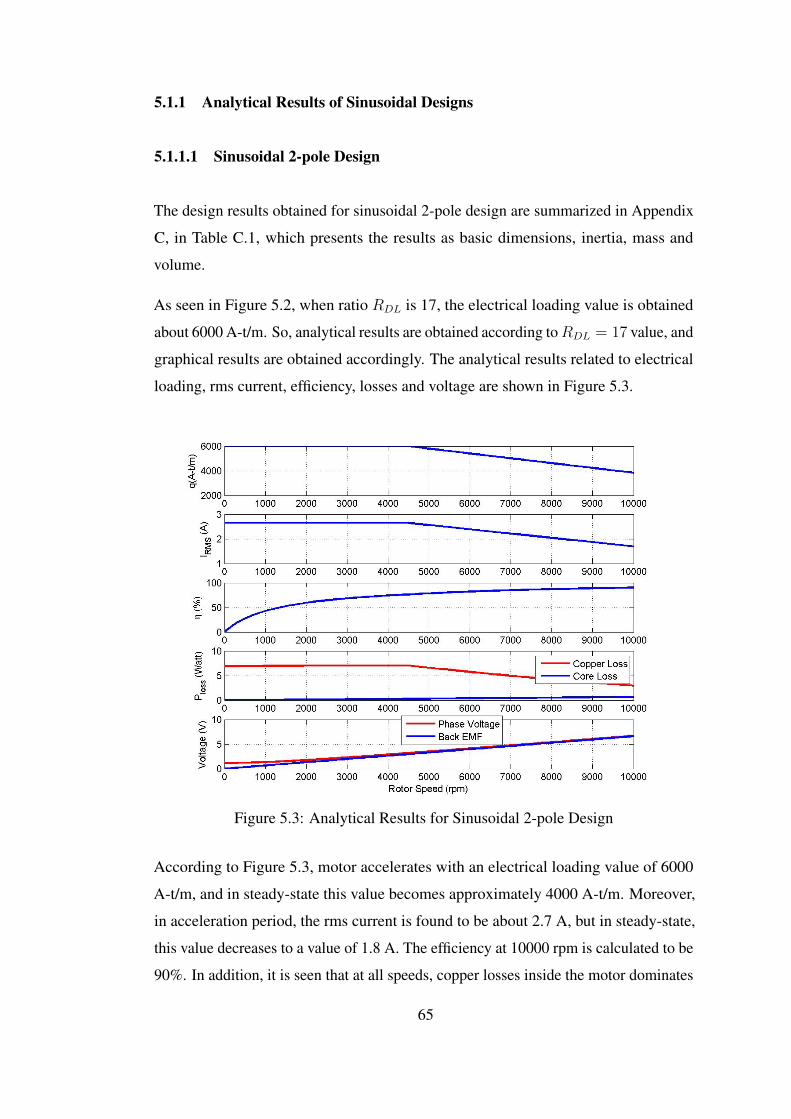
5.1.1 Analytical Results of Sinusoidal Designs

5.1.1.1 Sinusoidal 2-pole Design

The design results obtained for sinusoidal 2-pole design are summarized in Appendix

C, in Table C.1, which presents the results as basic dimensions, inertia, mass and

volume.

As seen in Figure 5.2, when ratio RDL is 17, the electrical loading value is obtained

about 6000 A-t/m. So, analytical results are obtained according toRDL = 17 value, and

graphical results are obtained accordingly. The analytical results related to electrical

loading, rms current, efficiency, losses and voltage are shown in Figure 5.3.

Figure 5.3: Analytical Results for Sinusoidal 2-pole Design

According to Figure 5.3, motor accelerates with an electrical loading value of 6000

A-t/m, and in steady-state this value becomes approximately 4000 A-t/m. Moreover,

in acceleration period, the rms current is found to be about 2.7 A, but in steady-state,

this value decreases to a value of 1.8 A. The efficiency at 10000 rpm is calculated to be

90%. In addition, it is seen that at all speeds, copper losses inside the motor dominates

65

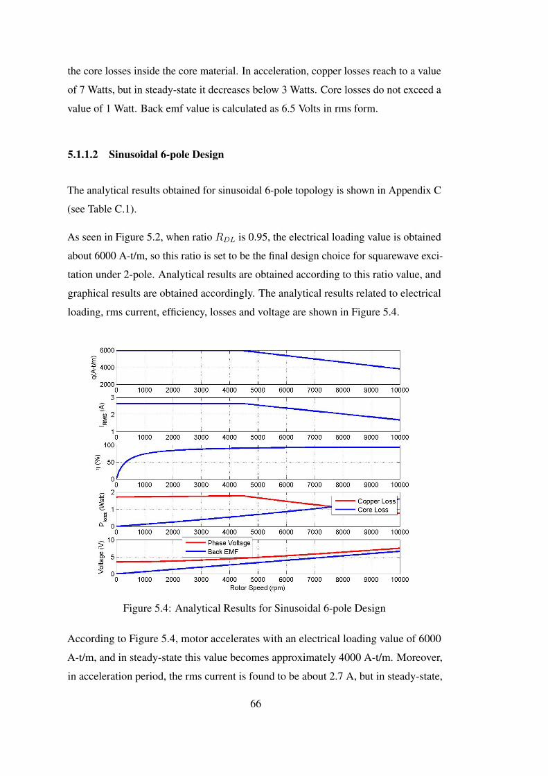
the core losses inside the core material. In acceleration, copper losses reach to a value

of 7 Watts, but in steady-state it decreases below 3 Watts. Core losses do not exceed a

value of 1 Watt. Back emf value is calculated as 6.5 Volts in rms form.

5.1.1.2 Sinusoidal 6-pole Design

The analytical results obtained for sinusoidal 6-pole topology is shown in Appendix C

(see Table C.1).

As seen in Figure 5.2, when ratio RDL is 0.95, the electrical loading value is obtained

about 6000 A-t/m, so this ratio is set to be the final design choice for squarewave exci-

tation under 2-pole. Analytical results are obtained according to this ratio value, and

graphical results are obtained accordingly. The analytical results related to electrical

loading, rms current, efficiency, losses and voltage are shown in Figure 5.4.

Figure 5.4: Analytical Results for Sinusoidal 6-pole Design

According to Figure 5.4, motor accelerates with an electrical loading value of 6000

A-t/m, and in steady-state this value becomes approximately 4000 A-t/m. Moreover,

in acceleration period, the rms current is found to be about 2.7 A, but in steady-state,

66

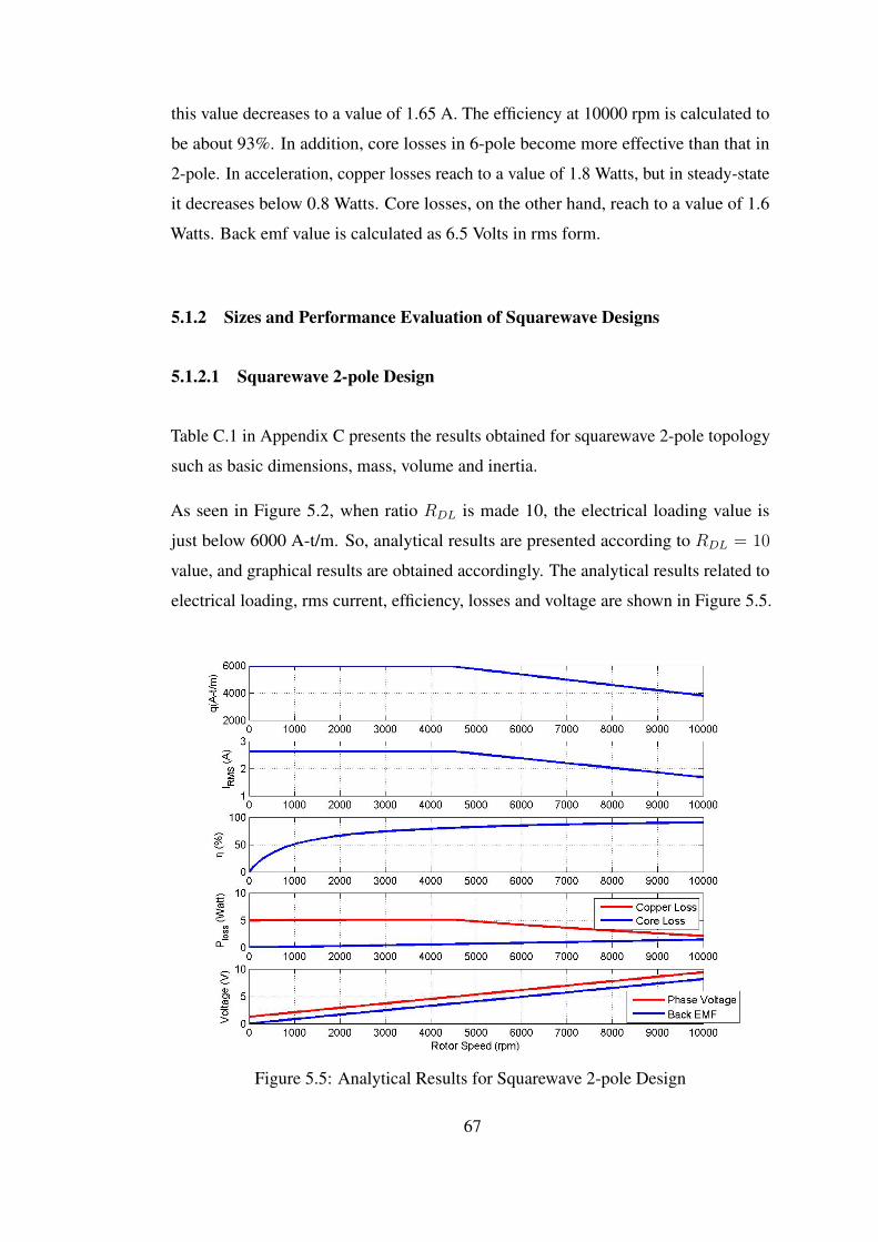
this value decreases to a value of 1.65 A. The efficiency at 10000 rpm is calculated to

be about 93%. In addition, core losses in 6-pole become more effective than that in

2-pole. In acceleration, copper losses reach to a value of 1.8 Watts, but in steady-state

it decreases below 0.8 Watts. Core losses, on the other hand, reach to a value of 1.6

Watts. Back emf value is calculated as 6.5 Volts in rms form.

5.1.2 Sizes and Performance Evaluation of Squarewave Designs

5.1.2.1 Squarewave 2-pole Design

Table C.1 in Appendix C presents the results obtained for squarewave 2-pole topology

such as basic dimensions, mass, volume and inertia.

As seen in Figure 5.2, when ratio RDL is made 10, the electrical loading value is

just below 6000 A-t/m. So, analytical results are presented according to RDL = 10

value, and graphical results are obtained accordingly. The analytical results related to

electrical loading, rms current, efficiency, losses and voltage are shown in Figure 5.5.

Figure 5.5: Analytical Results for Squarewave 2-pole Design

67

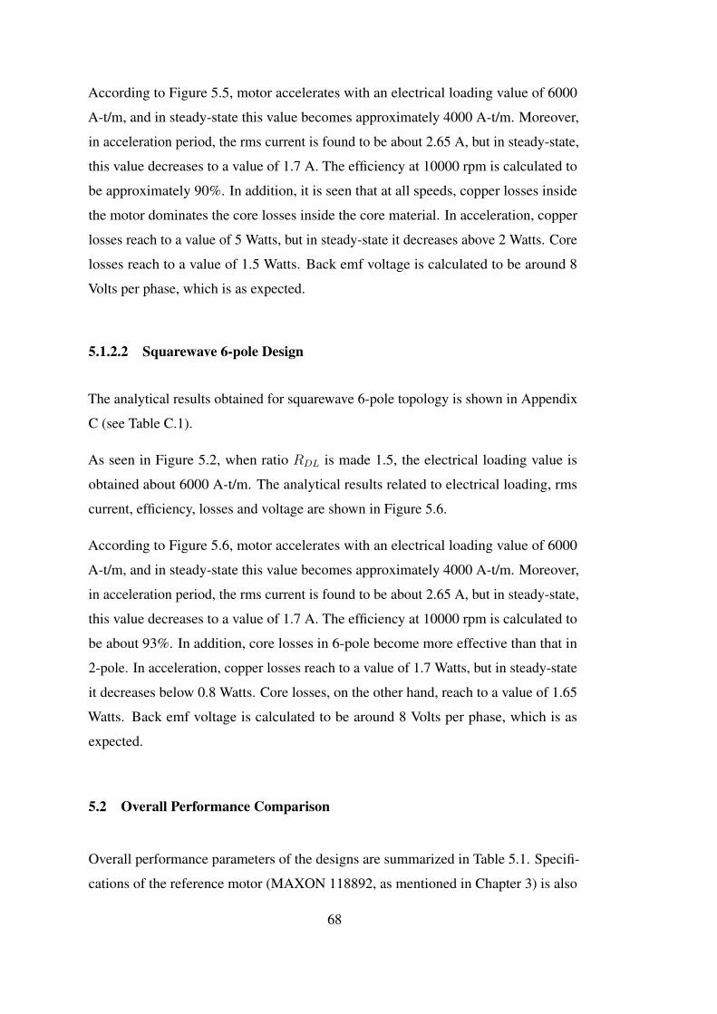
According to Figure 5.5, motor accelerates with an electrical loading value of 6000

A-t/m, and in steady-state this value becomes approximately 4000 A-t/m. Moreover,

in acceleration period, the rms current is found to be about 2.65 A, but in steady-state,

this value decreases to a value of 1.7 A. The efficiency at 10000 rpm is calculated to

be approximately 90%. In addition, it is seen that at all speeds, copper losses inside

the motor dominates the core losses inside the core material. In acceleration, copper

losses reach to a value of 5 Watts, but in steady-state it decreases above 2 Watts. Core

losses reach to a value of 1.5 Watts. Back emf voltage is calculated to be around 8

Volts per phase, which is as expected.

5.1.2.2 Squarewave 6-pole Design

The analytical results obtained for squarewave 6-pole topology is shown in Appendix

C (see Table C.1).

As seen in Figure 5.2, when ratio RDL is made 1.5, the electrical loading value is

obtained about 6000 A-t/m. The analytical results related to electrical loading, rms

current, efficiency, losses and voltage are shown in Figure 5.6.

According to Figure 5.6, motor accelerates with an electrical loading value of 6000

A-t/m, and in steady-state this value becomes approximately 4000 A-t/m. Moreover,

in acceleration period, the rms current is found to be about 2.65 A, but in steady-state,

this value decreases to a value of 1.7 A. The efficiency at 10000 rpm is calculated to

be about 93%. In addition, core losses in 6-pole become more effective than that in

2-pole. In acceleration, copper losses reach to a value of 1.7 Watts, but in steady-state

it decreases below 0.8 Watts. Core losses, on the other hand, reach to a value of 1.65

Watts. Back emf voltage is calculated to be around 8 Volts per phase, which is as

expected.

5.2 Overall Performance Comparison

Overall performance parameters of the designs are summarized in Table 5.1. Specifi-

cations of the reference motor (MAXON 118892, as mentioned in Chapter 3) is also

68

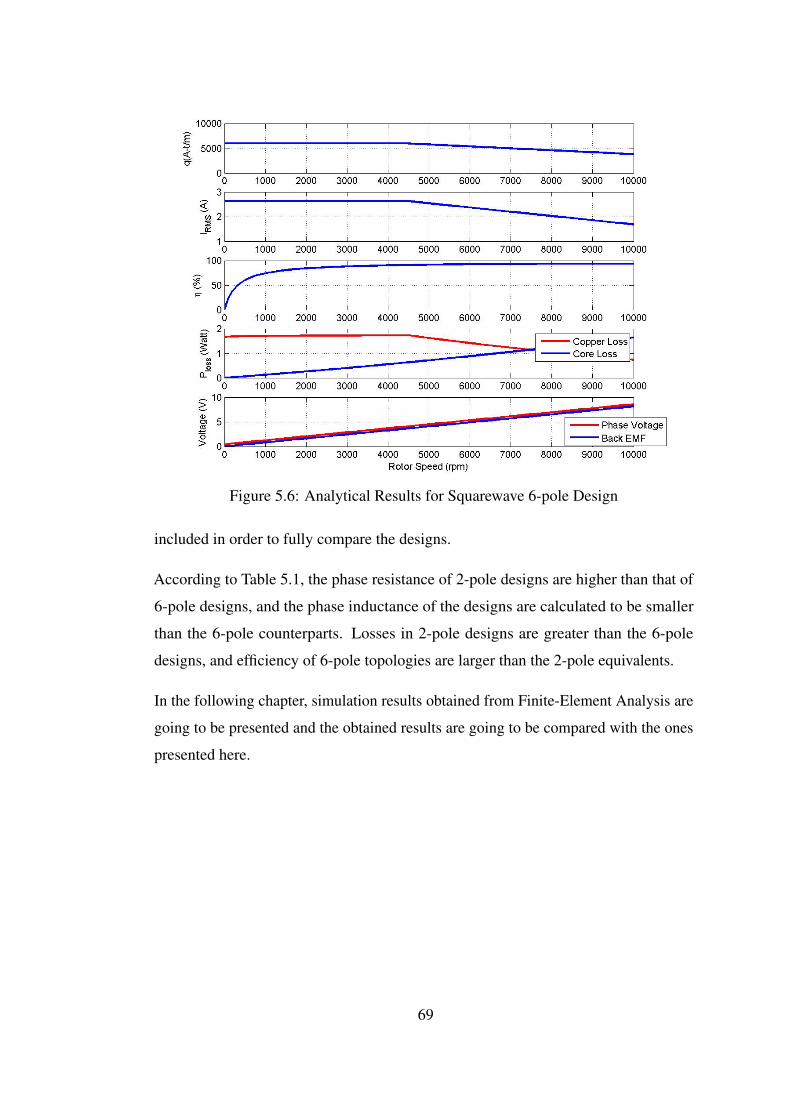
Figure 5.6: Analytical Results for Squarewave 6-pole Design

included in order to fully compare the designs.

According to Table 5.1, the phase resistance of 2-pole designs are higher than that of

6-pole designs, and the phase inductance of the designs are calculated to be smaller

than the 6-pole counterparts. Losses in 2-pole designs are greater than the 6-pole

designs, and efficiency of 6-pole topologies are larger than the 2-pole equivalents.

In the following chapter, simulation results obtained from Finite-Element Analysis are

going to be presented and the obtained results are going to be compared with the ones

presented here.

69

Table 5.1: Overall Performance Parameters at Steady-State

Parameter Sine2-pole

Sine6-pole

Square 2-pole

Square 6-pole

MAXON118892

Rph (mΩ) 327,45 82,73 238,38 80,30 481Lph (µH) 288,58 424,88 268,92 386,79 75Irms (A) 1,8 1,69 1,68 1,68 4,15eback−peak(V )

9,24 9,20 8 8 9

q (A.t/m) 4070 3795 3805 3847 -Bgav (T ) 0,43 0,43 0,43 0,43 -Bsbc−peak

(T )

1,45 1,46 1,43 1,44 -

PLoss (W ) 3,54 2,37 3,60 2,37 -η (%) 90,31 93,31 90,16 93,30 81τsteady−state(mN −m)

32 32 32 32 45,2

ns (rpm) 10000 10000 10000 10000 12700

70

CHAPTER 6

SIMULATION RESULTS

This chapter aims at verifying the analytical results obtained in Chapter 5. For this

purpose, Finite Element Analysis is made on the designs made in Chapter 4 and the

performance of the designs which are analytically made are compared with the results

found from the Finite-Element solution. Here, proper designs are chosen such that the

electrical loading value during the acceleration satisfies the design requirement, which

is 6000 A-t/m.

6.1 Simulation Results

As stated previously, ANSYS MAXWELL was used as the simulation tool for the

motors, as a Finite-Element Method solution tool. While solving the motors, the

meshes are assigned automatically by the program, so no additional assignment on

the meshes is made by the user in manual manner. In addition, core material and

permanent magnet properties are assigned as presented in Chapter 3. That is, a library

is constructed for both ferromagnetic material COGENT Power No. 12 by taking the

core loss data shown in Table 3.5 and Figure 3.9 and permanent magnet VACOMAX

225 HR as shown in 3.6. Core loss parameters and related B-H curves are entered

to the library, and stator and rotor materials are assigned accordingly, as well as

the assignment of permanent magnet material. The copper resistivity is taken as

1, 72.10−8Ω−m. Finally, transient solutions are applied in all motors. Boundaries are

assigned by the program automatically such that boundary conditions are defined just

outside the motor contour. In these regions, vector potential is taken to be zero, so no

71

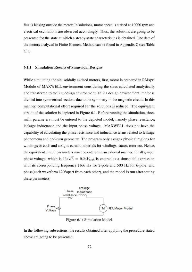
flux is leaking outside the motor. In solutions, motor speed is started at 10000 rpm and

electrical oscillations are observed accordingly. Thus, the solutions are going to be

presented for the state at which a steady-state characteristics is obtained. The data of

the motors analyzed in Finite-Element Method can be found in Appendix C (see Table

C.1).

6.1.1 Simulation Results of Sinusoidal Designs

While simulating the sinusoidally excited motors, first, motor is prepared in RMxprt

Module of MAXWELL environment considering the sizes calculated analytically

and transferred to the 2D design environment. In 2D design environment, motor is

divided into symmetrical sections due to the symmetry in the magnetic circuit. In this

manner, computational effort required for the solutions is reduced. The equivalent

circuit of the solution is depicted in Figure 6.1. Before running the simulation, three

main parameters must be entered to the depicted model, namely phase resistance,

leakage inductance and the input phase voltage. MAXWELL does not have the

capability of calculating the phase resistance and inductance terms related to leakage

phenomena and end-turn geometry. The program only assigns physical regions for

windings or coils and assigns certain materials for windings, stator, rotor etc. Hence,

the equivalent circuit parameters must be entered in an external manner. Finally, input

phase voltage, which is 16/√

3 = 9.24Vpeak is entered as a sinusoidal expression

with its corresponding frequency (166 Hz for 2-pole and 500 Hz for 6-pole) and

phase(each waveform 120°apart from each other), and the model is run after setting

these parameters.

Figure 6.1: Simulation Model

In the following subsections, the results obtained after applying the procedure stated

above are going to be presented.

72

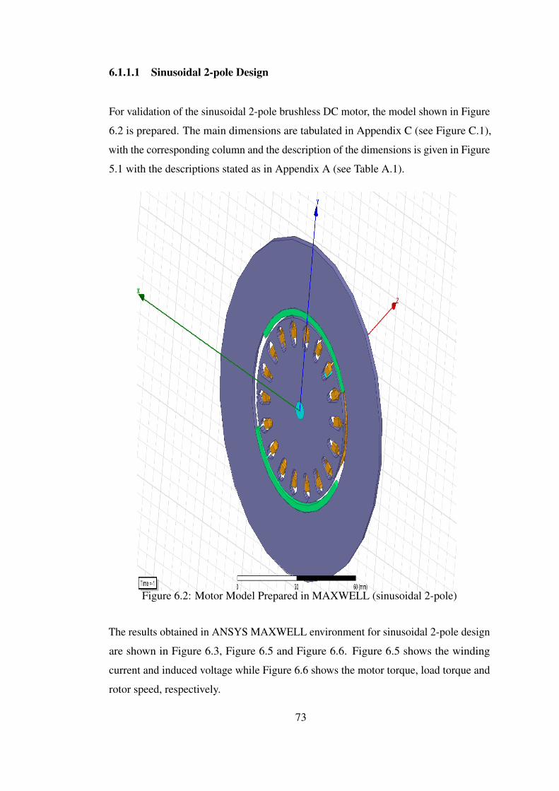
6.1.1.1 Sinusoidal 2-pole Design

For validation of the sinusoidal 2-pole brushless DC motor, the model shown in Figure

6.2 is prepared. The main dimensions are tabulated in Appendix C (see Figure C.1),

with the corresponding column and the description of the dimensions is given in Figure

5.1 with the descriptions stated as in Appendix A (see Table A.1).

Figure 6.2: Motor Model Prepared in MAXWELL (sinusoidal 2-pole)

The results obtained in ANSYS MAXWELL environment for sinusoidal 2-pole design

are shown in Figure 6.3, Figure 6.5 and Figure 6.6. Figure 6.5 shows the winding

current and induced voltage while Figure 6.6 shows the motor torque, load torque and

rotor speed, respectively.

73

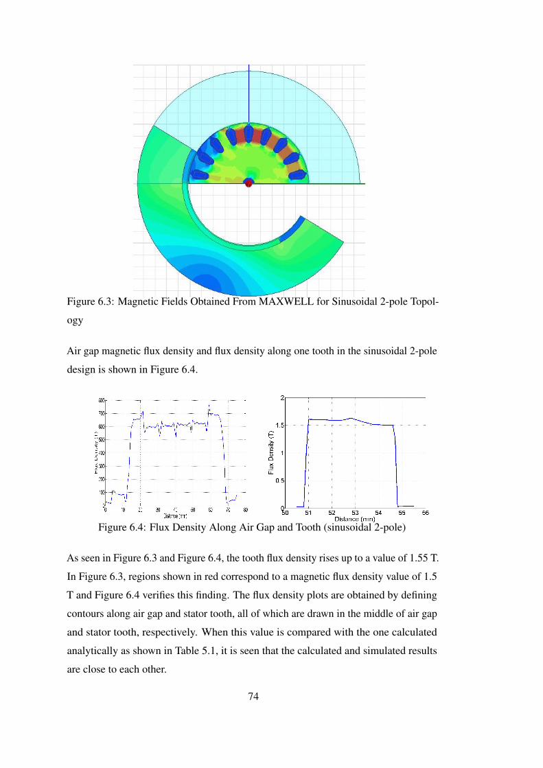
Figure 6.3: Magnetic Fields Obtained From MAXWELL for Sinusoidal 2-pole Topol-

ogy

Air gap magnetic flux density and flux density along one tooth in the sinusoidal 2-pole

design is shown in Figure 6.4.

Figure 6.4: Flux Density Along Air Gap and Tooth (sinusoidal 2-pole)

As seen in Figure 6.3 and Figure 6.4, the tooth flux density rises up to a value of 1.55 T.

In Figure 6.3, regions shown in red correspond to a magnetic flux density value of 1.5

T and Figure 6.4 verifies this finding. The flux density plots are obtained by defining

contours along air gap and stator tooth, all of which are drawn in the middle of air gap

and stator tooth, respectively. When this value is compared with the one calculated

analytically as shown in Table 5.1, it is seen that the calculated and simulated results

are close to each other.

74

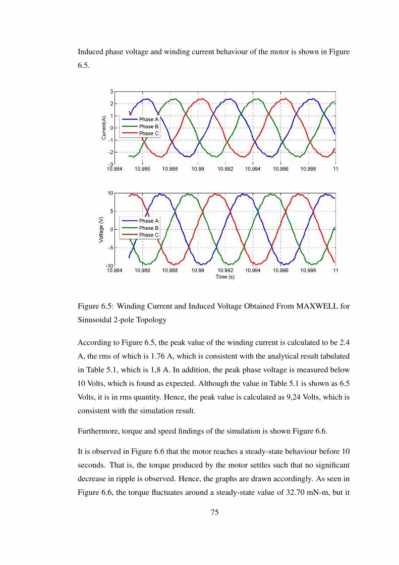
Induced phase voltage and winding current behaviour of the motor is shown in Figure

6.5.

Figure 6.5: Winding Current and Induced Voltage Obtained From MAXWELL for

Sinusoidal 2-pole Topology

According to Figure 6.5, the peak value of the winding current is calculated to be 2.4

A, the rms of which is 1.76 A, which is consistent with the analytical result tabulated

in Table 5.1, which is 1,8 A. In addition, the peak phase voltage is measured below

10 Volts, which is found as expected. Although the value in Table 5.1 is shown as 6.5

Volts, it is in rms quantity. Hence, the peak value is calculated as 9,24 Volts, which is

consistent with the simulation result.

Furthermore, torque and speed findings of the simulation is shown Figure 6.6.

It is observed in Figure 6.6 that the motor reaches a steady-state behaviour before 10

seconds. That is, the torque produced by the motor settles such that no significant

decrease in ripple is observed. Hence, the graphs are drawn accordingly. As seen in

Figure 6.6, the torque fluctuates around a steady-state value of 32.70 mN-m, but it

75

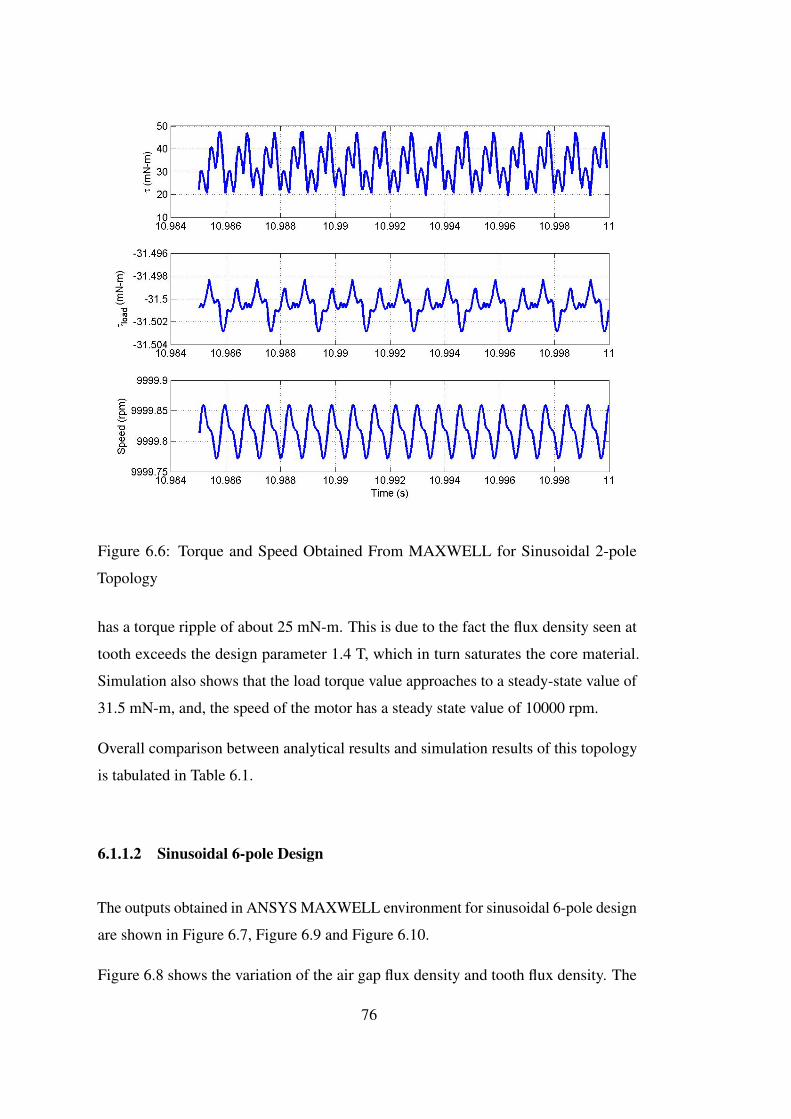
Figure 6.6: Torque and Speed Obtained From MAXWELL for Sinusoidal 2-pole

Topology

has a torque ripple of about 25 mN-m. This is due to the fact the flux density seen at

tooth exceeds the design parameter 1.4 T, which in turn saturates the core material.

Simulation also shows that the load torque value approaches to a steady-state value of

31.5 mN-m, and, the speed of the motor has a steady state value of 10000 rpm.

Overall comparison between analytical results and simulation results of this topology

is tabulated in Table 6.1.

6.1.1.2 Sinusoidal 6-pole Design

The outputs obtained in ANSYS MAXWELL environment for sinusoidal 6-pole design

are shown in Figure 6.7, Figure 6.9 and Figure 6.10.

Figure 6.8 shows the variation of the air gap flux density and tooth flux density. The

76

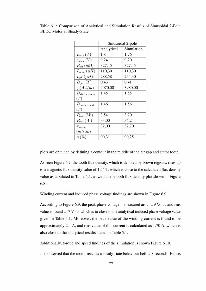
Table 6.1: Comparison of Analytical and Simulation Results of Sinusoidal 2-PoleBLDC Motor at Steady-State

Sinusoidal 2-poleAnalytical Simulation

Irms (A) 1,8 1,76eback (V ) 9,24 9,20Rph (mΩ) 327,45 327,45Lleak (µH) 110,30 110,30Lph (µH) 288,58 254,30Bgav (T ) 0,43 0,41q (A.t/m) 4070,00 3980,00Bstator−peak

(T )

1,45 1,55

Brotor−peak

(T )

1,46 1,56

Ploss (W ) 3,54 3,70Pout (W ) 33,00 34,24τmotor(mN.m)

32,00 32,70

η (%) 90,31 90,25

plots are obtained by defining a contour in the middle of the air gap and stator tooth.

As seen Figure 6.7, the tooth flux density, which is denoted by brown regions, rises up

to a magnetic flux density value of 1.54 T, which is close to the calculated flux density

value as tabulated in Table 5.1, as well as thetooth flux density plot shown in Figure

6.8.

Winding current and induced phase voltage findings are shown in Figure 6.9.

According to Figure 6.9, the peak phase voltage is measured around 9 Volts, and rms

value is found as 7 Volts which is to close to the analytical induced phase voltage value

given in Table 5.1. Moreover, the peak value of the winding current is found to be

approximately 2.4 A, and rms value of this current is calculated as 1.70 A, which is

also close to the analytical results stated in Table 5.1.

Additionally, torque and speed findings of the simulation is shown Figure 6.10.

It is observed that the motor reaches a steady-state behaviour before 8 seconds. Hence,

77

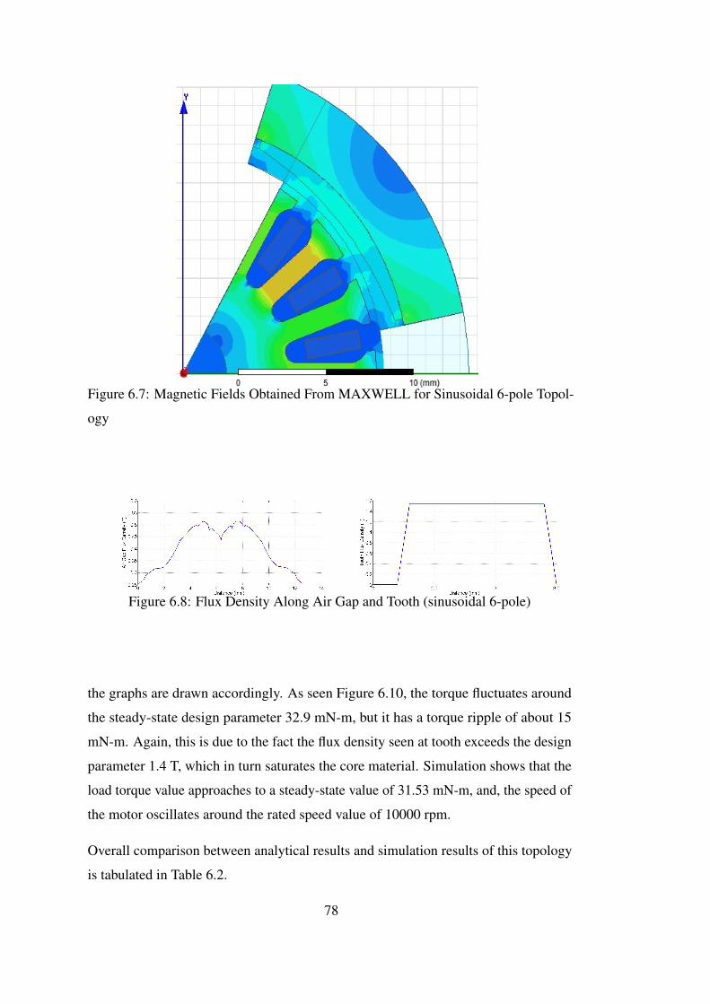
Figure 6.7: Magnetic Fields Obtained From MAXWELL for Sinusoidal 6-pole Topol-

ogy

Figure 6.8: Flux Density Along Air Gap and Tooth (sinusoidal 6-pole)

the graphs are drawn accordingly. As seen Figure 6.10, the torque fluctuates around

the steady-state design parameter 32.9 mN-m, but it has a torque ripple of about 15

mN-m. Again, this is due to the fact the flux density seen at tooth exceeds the design

parameter 1.4 T, which in turn saturates the core material. Simulation shows that the

load torque value approaches to a steady-state value of 31.53 mN-m, and, the speed of

the motor oscillates around the rated speed value of 10000 rpm.

Overall comparison between analytical results and simulation results of this topology

is tabulated in Table 6.2.

78

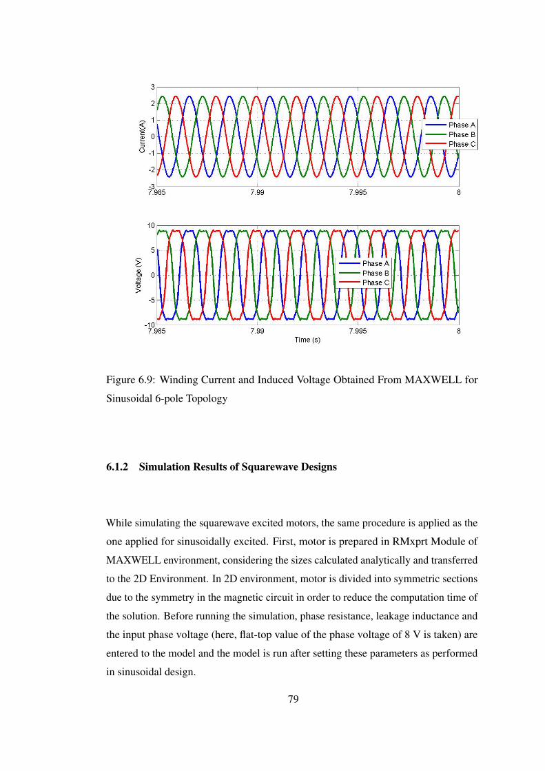
Figure 6.9: Winding Current and Induced Voltage Obtained From MAXWELL for

Sinusoidal 6-pole Topology

6.1.2 Simulation Results of Squarewave Designs

While simulating the squarewave excited motors, the same procedure is applied as the

one applied for sinusoidally excited. First, motor is prepared in RMxprt Module of

MAXWELL environment, considering the sizes calculated analytically and transferred

to the 2D Environment. In 2D environment, motor is divided into symmetric sections

due to the symmetry in the magnetic circuit in order to reduce the computation time of

the solution. Before running the simulation, phase resistance, leakage inductance and

the input phase voltage (here, flat-top value of the phase voltage of 8 V is taken) are

entered to the model and the model is run after setting these parameters as performed

in sinusoidal design.

79

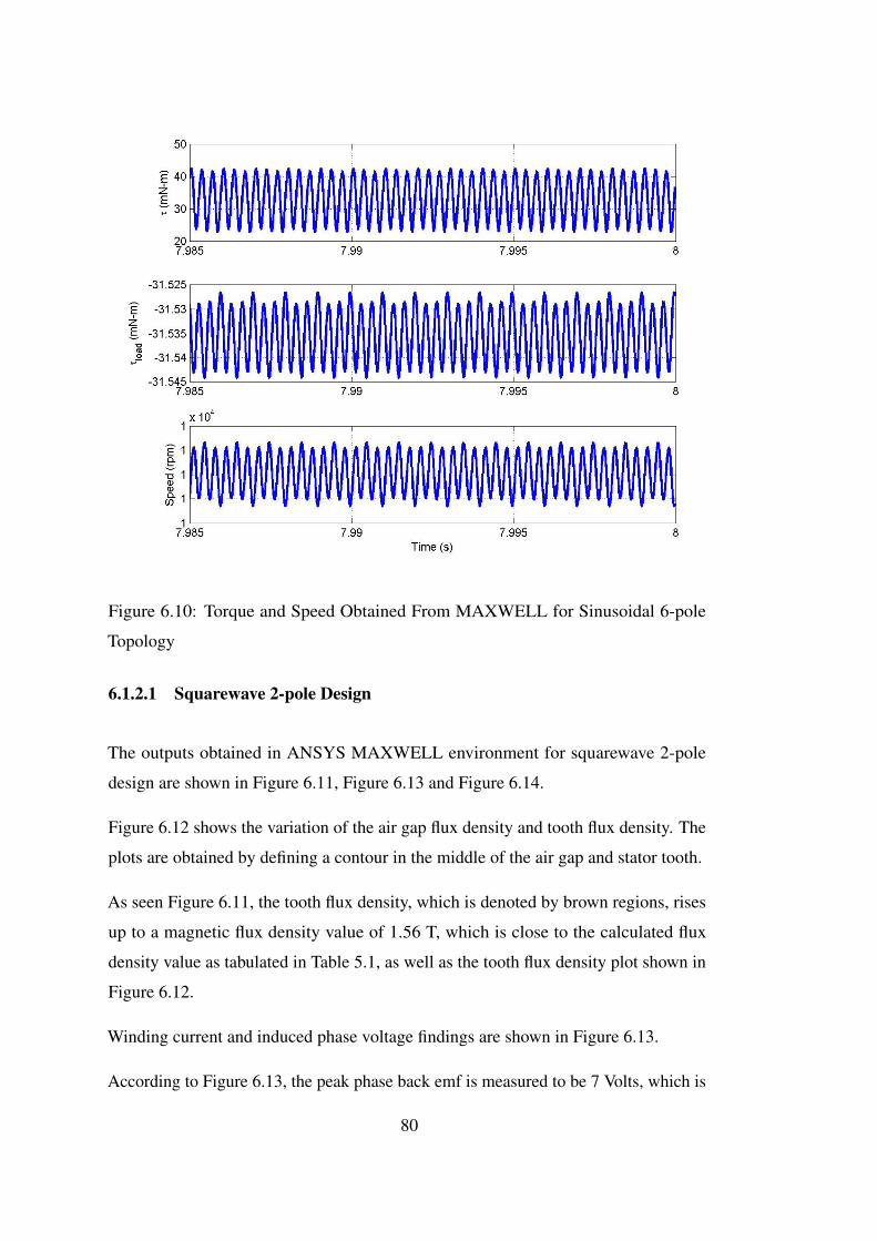
Figure 6.10: Torque and Speed Obtained From MAXWELL for Sinusoidal 6-pole

Topology

6.1.2.1 Squarewave 2-pole Design

The outputs obtained in ANSYS MAXWELL environment for squarewave 2-pole

design are shown in Figure 6.11, Figure 6.13 and Figure 6.14.

Figure 6.12 shows the variation of the air gap flux density and tooth flux density. The

plots are obtained by defining a contour in the middle of the air gap and stator tooth.

As seen Figure 6.11, the tooth flux density, which is denoted by brown regions, rises

up to a magnetic flux density value of 1.56 T, which is close to the calculated flux

density value as tabulated in Table 5.1, as well as the tooth flux density plot shown in

Figure 6.12.

Winding current and induced phase voltage findings are shown in Figure 6.13.

According to Figure 6.13, the peak phase back emf is measured to be 7 Volts, which is

80

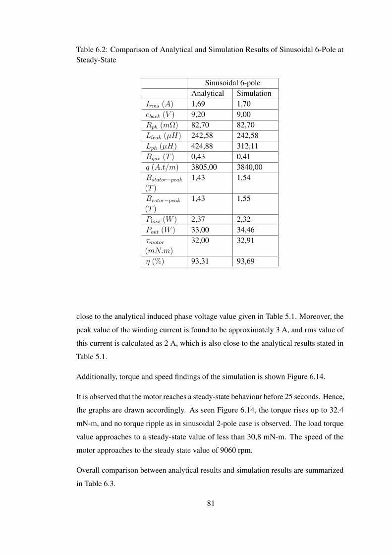
Table 6.2: Comparison of Analytical and Simulation Results of Sinusoidal 6-Pole atSteady-State

Sinusoidal 6-poleAnalytical Simulation

Irms (A) 1,69 1,70eback (V ) 9,20 9,00Rph (mΩ) 82,70 82,70Lleak (µH) 242,58 242,58Lph (µH) 424,88 312,11Bgav (T ) 0,43 0,41q (A.t/m) 3805,00 3840,00Bstator−peak

(T )

1,43 1,54

Brotor−peak

(T )

1,43 1,55

Ploss (W ) 2,37 2,32Pout (W ) 33,00 34,46τmotor(mN.m)

32,00 32,91

η (%) 93,31 93,69

close to the analytical induced phase voltage value given in Table 5.1. Moreover, the

peak value of the winding current is found to be approximately 3 A, and rms value of

this current is calculated as 2 A, which is also close to the analytical results stated in

Table 5.1.

Additionally, torque and speed findings of the simulation is shown Figure 6.14.

It is observed that the motor reaches a steady-state behaviour before 25 seconds. Hence,

the graphs are drawn accordingly. As seen Figure 6.14, the torque rises up to 32.4

mN-m, and no torque ripple as in sinusoidal 2-pole case is observed. The load torque

value approaches to a steady-state value of less than 30,8 mN-m. The speed of the

motor approaches to the steady state value of 9060 rpm.

Overall comparison between analytical results and simulation results are summarized

in Table 6.3.

81

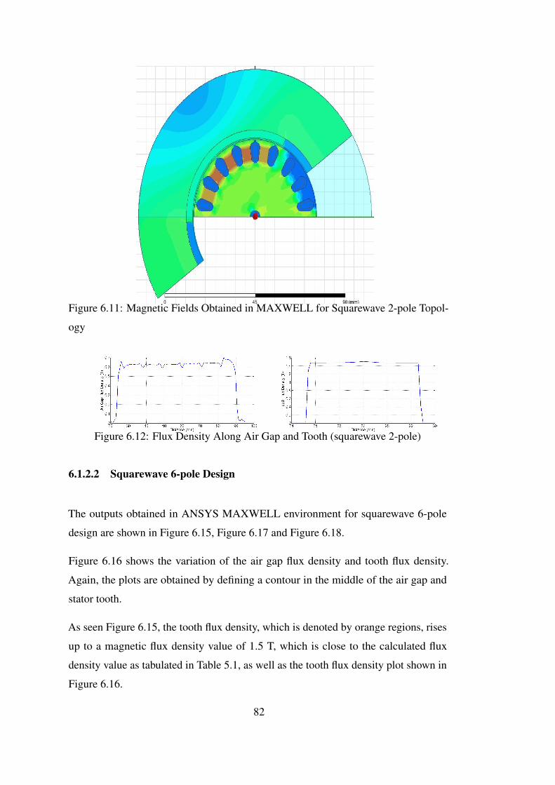
Figure 6.11: Magnetic Fields Obtained in MAXWELL for Squarewave 2-pole Topol-

ogy

Figure 6.12: Flux Density Along Air Gap and Tooth (squarewave 2-pole)

6.1.2.2 Squarewave 6-pole Design

The outputs obtained in ANSYS MAXWELL environment for squarewave 6-pole

design are shown in Figure 6.15, Figure 6.17 and Figure 6.18.

Figure 6.16 shows the variation of the air gap flux density and tooth flux density.

Again, the plots are obtained by defining a contour in the middle of the air gap and

stator tooth.

As seen Figure 6.15, the tooth flux density, which is denoted by orange regions, rises

up to a magnetic flux density value of 1.5 T, which is close to the calculated flux

density value as tabulated in Table 5.1, as well as the tooth flux density plot shown in

Figure 6.16.

82

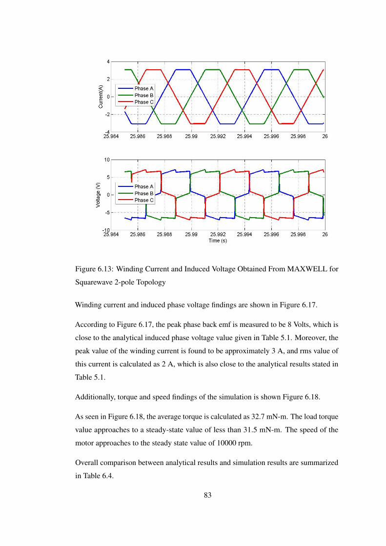
Figure 6.13: Winding Current and Induced Voltage Obtained From MAXWELL for

Squarewave 2-pole Topology

Winding current and induced phase voltage findings are shown in Figure 6.17.

According to Figure 6.17, the peak phase back emf is measured to be 8 Volts, which is

close to the analytical induced phase voltage value given in Table 5.1. Moreover, the

peak value of the winding current is found to be approximately 3 A, and rms value of

this current is calculated as 2 A, which is also close to the analytical results stated in

Table 5.1.

Additionally, torque and speed findings of the simulation is shown Figure 6.18.

As seen in Figure 6.18, the average torque is calculated as 32.7 mN-m. The load torque

value approaches to a steady-state value of less than 31.5 mN-m. The speed of the

motor approaches to the steady state value of 10000 rpm.

Overall comparison between analytical results and simulation results are summarized

in Table 6.4.

83

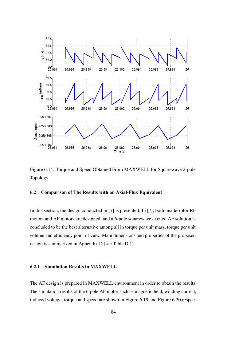
Figure 6.14: Torque and Speed Obtained From MAXWELL for Squarewave 2-pole

Topology

6.2 Comparison of The Results with an Axial-Flux Equivalent

In this section, the design conducted in [7] is presented. In [7], both inside-rotor RF

motors and AF motors are designed, and a 6-pole squarewave excited AF solution is

concluded to be the best alternative among all in torque per unit mass, torque per unit

volume and efficiency point of view. Main dimensions and properties of the proposed

design is summarized in Appendix D (see Table D.1).

6.2.1 Simulation Results in MAXWELL

The AF design is prepared in MAXWELL environment in order to obtain the results.

The simulation results of the 6-pole AF motor such as magnetic field, winding current,

induced voltage, torque and speed are shown in Figure 6.19 and Figure 6.20,respec-

84

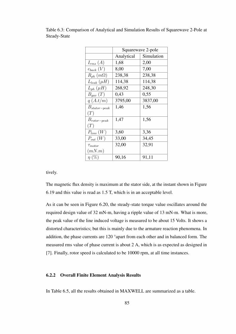
Table 6.3: Comparison of Analytical and Simulation Results of Squarewave 2-Pole atSteady-State

Squarewave 2-poleAnalytical Simulation

Irms (A) 1,68 2,00eback (V ) 8,00 7,00Rph (mΩ) 238,38 238,38Lleak (µH) 114,38 114,38Lph (µH) 268,92 248,30Bgav (T ) 0,43 0,55q (A.t/m) 3795,00 3837,00Bstator−peak

(T )

1,46 1,56

Brotor−peak

(T )

1,47 1,56

Ploss (W ) 3,60 3,36Pout (W ) 33,00 34,45τmotor(mN.m)

32,00 32,91

η (%) 90,16 91,11

tively.

The magnetic flux density is maximum at the stator side, at the instant shown in Figure

6.19 and this value is read as 1.5 T, which is in an acceptable level.

As it can be seen in Figure 6.20, the steady-state torque value oscillates around the

required design value of 32 mN-m, having a ripple value of 13 mN-m. What is more,

the peak value of the line induced voltage is measured to be about 15 Volts. It shows a

distorted characteristics; but this is mainly due to the armature reaction phenomena. In

addition, the phase currents are 120 °apart from each other and in balanced form. The

measured rms value of phase current is about 2 A, which is as expected as designed in

[7]. Finally, rotor speed is calculated to be 10000 rpm, at all time instances.

6.2.2 Overall Finite Element Analysis Results

In Table 6.5, all the results obtained in MAXWELL are summarized as a table.

85

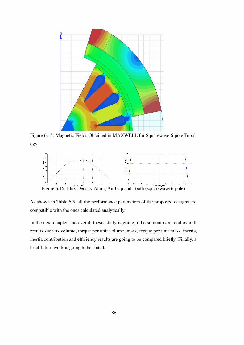
Figure 6.15: Magnetic Fields Obtained in MAXWELL for Squarewave 6-pole Topol-

ogy

Figure 6.16: Flux Density Along Air Gap and Tooth (squarewave 6-pole)

As shown in Table 6.5, all the performance parameters of the proposed designs are

compatible with the ones calculated analytically.

In the next chapter, the overall thesis study is going to be summarized, and overall

results such as volume, torque per unit volume, mass, torque per unit mass, inertia,

inertia contribution and efficiency results are going to be compared briefly. Finally, a

brief future work is going to be stated.

86

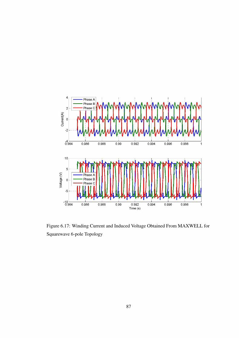
Figure 6.17: Winding Current and Induced Voltage Obtained From MAXWELL for

Squarewave 6-pole Topology

87

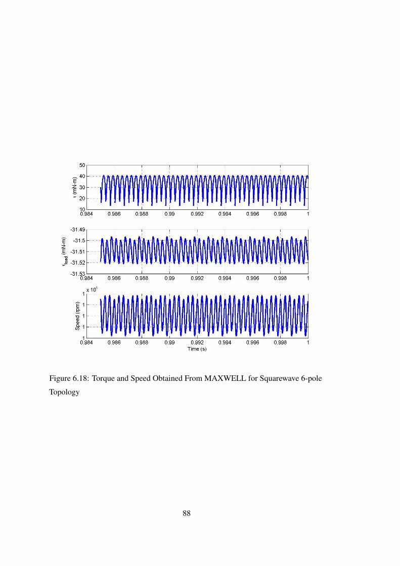
Figure 6.18: Torque and Speed Obtained From MAXWELL for Squarewave 6-pole

Topology

88

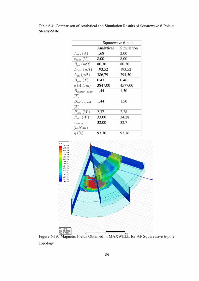
Table 6.4: Comparison of Analytical and Simulation Results of Squarewave 6-Pole atSteady-State

Squarewave 6-poleAnalytical Simulation

Irms (A) 1,68 2,00eback (V ) 8,00 8,00Rph (mΩ) 80,30 80,30Lleak (µH) 193,52 193,52Lph (µH) 386,79 294,50Bgav (T ) 0,43 0,46q (A.t/m) 3847,00 4577,00Bstator−peak

(T )

1,44 1,50

Brotor−peak

(T )

1,44 1,50

Ploss (W ) 2,37 2,28Pout (W ) 33,00 34,28τmotor(mN.m)

32,00 32,7

η (%) 93,30 93,76

Figure 6.19: Magnetic Fields Obtained in MAXWELL for AF Squarewave 6-pole

Topology

89

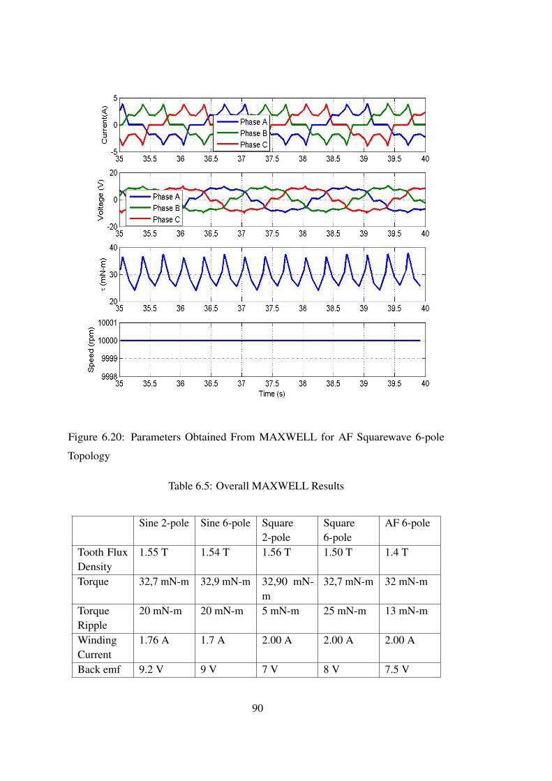
Figure 6.20: Parameters Obtained From MAXWELL for AF Squarewave 6-pole

Topology

Table 6.5: Overall MAXWELL Results

Sine 2-pole Sine 6-pole Square2-pole

Square6-pole

AF 6-pole

Tooth FluxDensity

1.55 T 1.54 T 1.56 T 1.50 T 1.4 T

Torque 32,7 mN-m 32,9 mN-m 32,90 mN-m

32,7 mN-m 32 mN-m

TorqueRipple

20 mN-m 20 mN-m 5 mN-m 25 mN-m 13 mN-m

WindingCurrent

1.76 A 1.7 A 2.00 A 2.00 A 2.00 A

Back emf 9.2 V 9 V 7 V 8 V 7.5 V

90

CHAPTER 7

CONCLUSION

This chapter briefly wraps up all the results obtained and stated in Chapter 5 and

Chapter 6, and makes deductions about the future work that can be derived afterwards.

7.1 Overall Results

In this thesis study, an alternative motor topology is proposed for Control Moment

Gyroscope applications, which is a crucial inertial system in a satellite. For this

purpose, first operation principle of CMGs is stated and typical electrical motors used

in an aerospace application are defined. Then, brushless DC motors are classified

depending on the permanent magnet location, flux direction and excitation. Problems in

the current CMG prototypes are defined and motor selection criteria is stated in Chapter

3. In Chapter 4, outer-rotor brushless DC motor design procedure is explained and the

first results are illustrated. In Chapter 5, a design is chosen for each topology, namely

for excitation and pole number and results obtained analytically are investigated. In

Chapter 6, the design set is prepared for validation under Finite-Element Analysis

and simulation results are illustrated, as well as the design conducted by [7]. Overall

results are summarized below.

Overall volume comparison is shown Figure 7.1.

As shown in Figure 7.1, volume comparison is made both with volume and torque per

unit volume. If volume is investigated, it is concluded that 6-pole designs are smaller

in volume when compared to the 2-pole designs. This fact leads to the explanation of

91

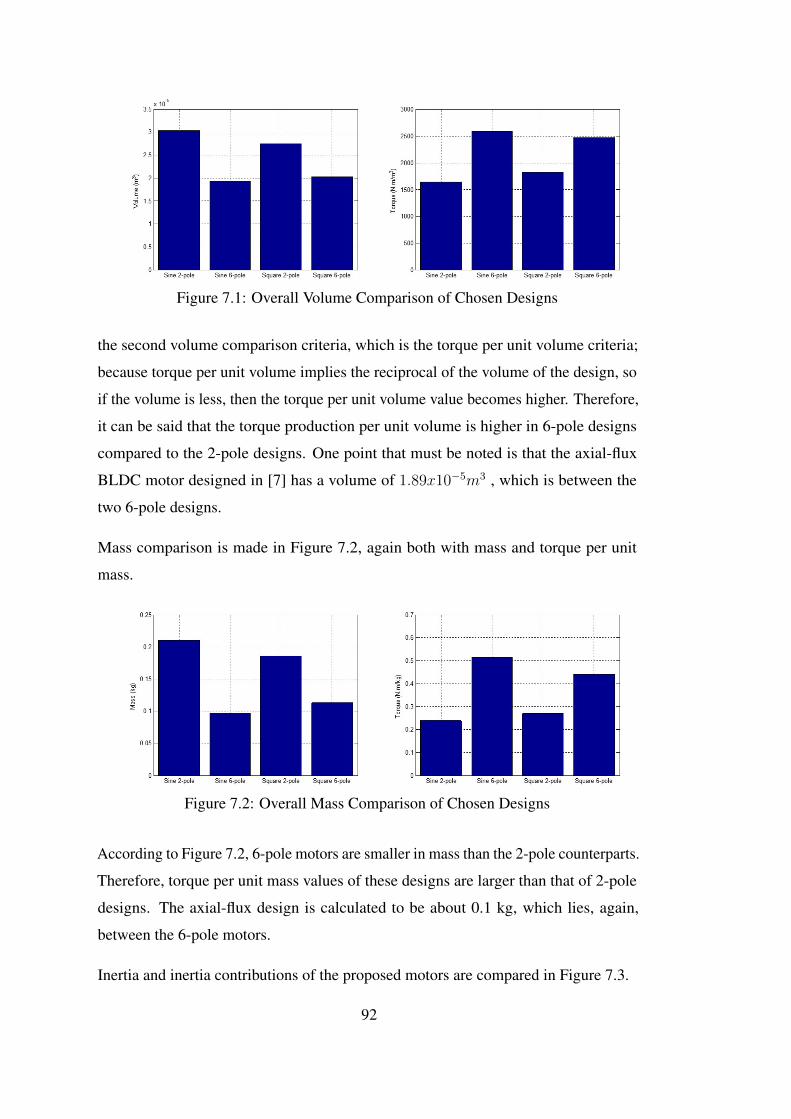
Figure 7.1: Overall Volume Comparison of Chosen Designs

the second volume comparison criteria, which is the torque per unit volume criteria;

because torque per unit volume implies the reciprocal of the volume of the design, so

if the volume is less, then the torque per unit volume value becomes higher. Therefore,

it can be said that the torque production per unit volume is higher in 6-pole designs

compared to the 2-pole designs. One point that must be noted is that the axial-flux

BLDC motor designed in [7] has a volume of 1.89x10−5m3 , which is between the

two 6-pole designs.

Mass comparison is made in Figure 7.2, again both with mass and torque per unit

mass.

Figure 7.2: Overall Mass Comparison of Chosen Designs

According to Figure 7.2, 6-pole motors are smaller in mass than the 2-pole counterparts.

Therefore, torque per unit mass values of these designs are larger than that of 2-pole

designs. The axial-flux design is calculated to be about 0.1 kg, which lies, again,

between the 6-pole motors.

Inertia and inertia contributions of the proposed motors are compared in Figure 7.3.

92

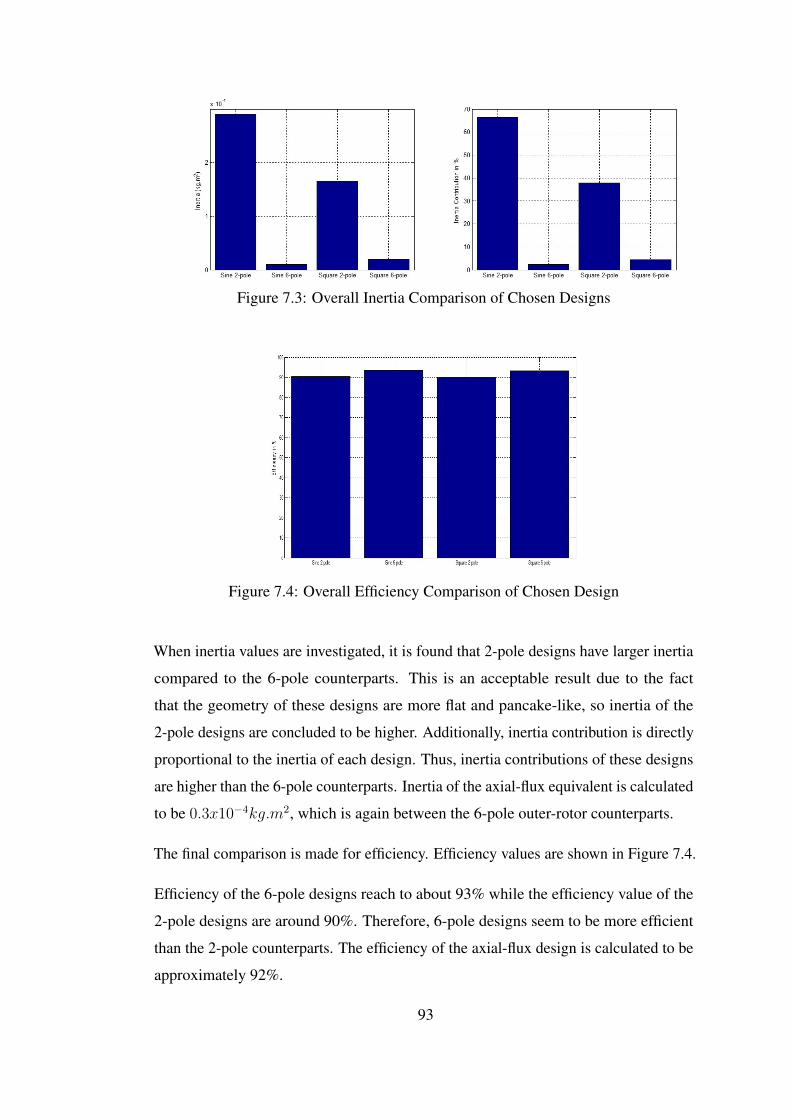
Figure 7.3: Overall Inertia Comparison of Chosen Designs

Figure 7.4: Overall Efficiency Comparison of Chosen Design

When inertia values are investigated, it is found that 2-pole designs have larger inertia

compared to the 6-pole counterparts. This is an acceptable result due to the fact

that the geometry of these designs are more flat and pancake-like, so inertia of the

2-pole designs are concluded to be higher. Additionally, inertia contribution is directly

proportional to the inertia of each design. Thus, inertia contributions of these designs

are higher than the 6-pole counterparts. Inertia of the axial-flux equivalent is calculated

to be 0.3x10−4kg.m2, which is again between the 6-pole outer-rotor counterparts.

The final comparison is made for efficiency. Efficiency values are shown in Figure 7.4.

Efficiency of the 6-pole designs reach to about 93% while the efficiency value of the

2-pole designs are around 90%. Therefore, 6-pole designs seem to be more efficient

than the 2-pole counterparts. The efficiency of the axial-flux design is calculated to be

approximately 92%.

93

As final remarks with the axial-flux design, it can be said that the mass of the 6-pole

squarewave RF outer-rotor motor solution is slightly heavier than the AF solution and

its volume is less than AF solution. Mass and volume calculation is made, considering

only the active material mass and volume of the motors. This however is of secondary

importance. What matters is the mass and volume of the system when it is configured

to have the required inertia. One must note here that the RF motor solution has a large

diameter and is thin. The contribution of the motor inertia to the required inertia is

about 2% of the total, while for the AF solution this ratio is 6%.

To conclude the results, 6-pole designs can be preferred if higher torque per unit

mass or volume with higher efficiency is desired. On the other hand, if larger inertia

contributions are desired in the system design, 2-pole designs can be preferred.

7.2 Future Work

Possible future work areas that can be derived from this work are summarized as

follows:

• It must be noted that, although the temperature model is presented in Chapter

3, the temperature characteristics are not deeply studied. The main point of

consideration is that since these motors are intended to be used in a satellite

application, cooling techniques must be well handled regarding heat transfer

by conduction or by radiation. Here, materials are selected depending on the

radiation sensitivity. Yet, cooling issue must not be ignored during an integration

of such motors to the system.

• Although inertia contributions are mentioned in this study, proper integration of

the motors of interest are not included in the thesis. A detailed investigation on

this issue must be carried out in order to fully understand the volumetric cost of

the electrical motors to the whole CMG system.

• Since the motors are designed in surface-mounted magnet topology, the mechan-

ical considerations can be further investigated. In order to protect magnets from

detachment, a non-magnetic ring can be put inside the magnet surface, which

94

may be counted as a solution for the mentioned issue.

• Further designs can be studied by considering torque minimization techniques

such as skewing and pole arcing. Improving the torque ripple ratings of the

designs may lead to a better wheel motor design for a typical CMG application.

• The design can be handled using multi-objective optimization techniques in

order to further minimize the mass and volume by defining certain constraints

such as electrical loading, air gap magnetic flux density and current density.

95

96

REFERENCES

[1] Public lessons learned entry 0893. http://www.nasa.gov/offices/oce/llis/0893.html. Accessed: 19/09/2014.

[2] Vacomax 225 hr properties. http://www.vacuumschmelze.com/en/products/permanent_magnets_assemblies/permanent_magnets/sm_co/vacomax/vacomax_225_hr.html. Accessed:10/08/2014.

[3] Douglas D. Havenhill. Direct torque control moment gyroscope, February 1995.

[4] V.J. Lappas, W.H. Steyn, and C.I. Underwood. Attitude control for small satellitesusing control moment gyros. Acta Astronautica, 51(1-9):101–111, July 2002.

[5] X Roser and M Sghedoni. Control moment gyroscopes (cmg’s) and their ap-plication in future scientific missions. In Spacecraft Guidance, Navigation andControl Systems, volume 381, page 523, 1997.

[6] D.C. Hanselman. Brushless Permanent Magnet Motor Design. Magna PhysicsPublishing, 2006.

[7] Kurtulus Yılmaz. Comparison of axial flux and radial flux brushless dc motortopologies for control moment gyroscope wheel applications. Master’s thesis,Middle East Technical University, April 2009.

[8] N. Mohan. Electric Machines and Drives. CourseSmart Series. Wiley, 2012.

[9] Vaios J. Lappas. A Control Moment Gyro (CMG) Based Attitude Control System(ACS) for Agile Small Satellites. PhD thesis, University of Surrey, October 2002.

[10] W Jaffe and TJ Sokira. Brushless dc motors: Electronics commutation andcontrol, 1990.

[11] Padmaraja Yedamale. Brushless dc (bldc) motor fundamentals. MicrochipTechnology Inc, page 20, 2003.

[12] David G Dorrell, M Hsieh, Mircea Popescu, Lyndon Evans, David A Staton, andVic Grout. A review of the design issues and techniques for radial-flux brushlesssurface and internal rare-earth permanent-magnet motors. Industrial Electronics,IEEE Transactions on, 58(9):3741–3757, 2011.

97

[13] F Sahin, AM Tuckey, and AJA Vandenput. Design, development and testing ofa high-speed axial-flux permanent-magnet machine. In Industry ApplicationsConference, 2001. Thirty-Sixth IAS Annual Meeting. Conference Record of the2001 IEEE, volume 3, pages 1640–1647. IEEE, 2001.

[14] T.J.E. Miller. Brushless permanent-magnet and reluctance motor drives. Mono-graphs in electrical and electronic engineering. Clarendon Press, 1989.

[15] A. Cavagnino, M. Lazzari, F. Profumo, and A. Tenconi. A comparison betweenthe axial flux and the radial flux structures for pm synchronous motors. In Indus-try Applications Conference, 2001. Thirty-Sixth IAS Annual Meeting. ConferenceRecord of the 2001 IEEE, volume 3, pages 1611–1618 vol.3, Sept 2001.

[16] H.B. Ertan and K. Yilmaz. Choice of pole number of two-rotor axial-flux pmmotor for control moment gyroscope. In Electrical Machines and Power Elec-tronics and 2011 Electromotion Joint Conference (ACEMP), 2011 InternationalAegean Conference on, pages 620–625, Sept 2011.

[17] Dean J. Patterson, Jessica L. Colton, Brad Mularcik, Byron J. Kennedy, StevenCamilleri, and Rafal Rohoza. A comparison of radial and axial flux structuresin electrical machines. 2009 IEEE International Electric Machines and DrivesConference, pages 1029–1035, May 2009.

[18] Z Rahman. Evaluating radial, axial and transverse flux topologies for’in-wheel’motor. In Power Electronics in Transportation, 2004, pages 75–81. IEEE,2004.

[19] Gordon R Slemon. On the design of high-performance surface-mounted pmmotors. Industry Applications, IEEE Transactions on, 30(1):134–140, 1994.

[20] Nicola Bianchi and Silverio Bolognani. Design techniques for reducing thecogging torque in surface-mounted pm motors. Industry Applications, IEEETransactions on, 38(5):1259–1265, 2002.

[21] Emre Yavuzoglu. Steering laws for control moment gyroscope systems used inspacecraft attitude control. Master’s thesis, Middle East Technical University,November 2003.

[22] H.B. Ertan and N. Cagan. Comparison of outer rotor radial flux and axial flux pmmotors for cmg application. In Electrical Machines (ICEM), 2014 InternationalConference on, pages 1031–1036, Sept 2014.

[23] C.A. Gross. Electric Machines. Electric Power Engineering Series. Taylor &Francis, 2006.

98

APPENDIX A

PARAMETERS AND DESCRIPTIONS

Table A.1 shows the parameters and descriptions used throughout the thesis study.

Other tables regarding the dimensions are prepared by considering this table.

99

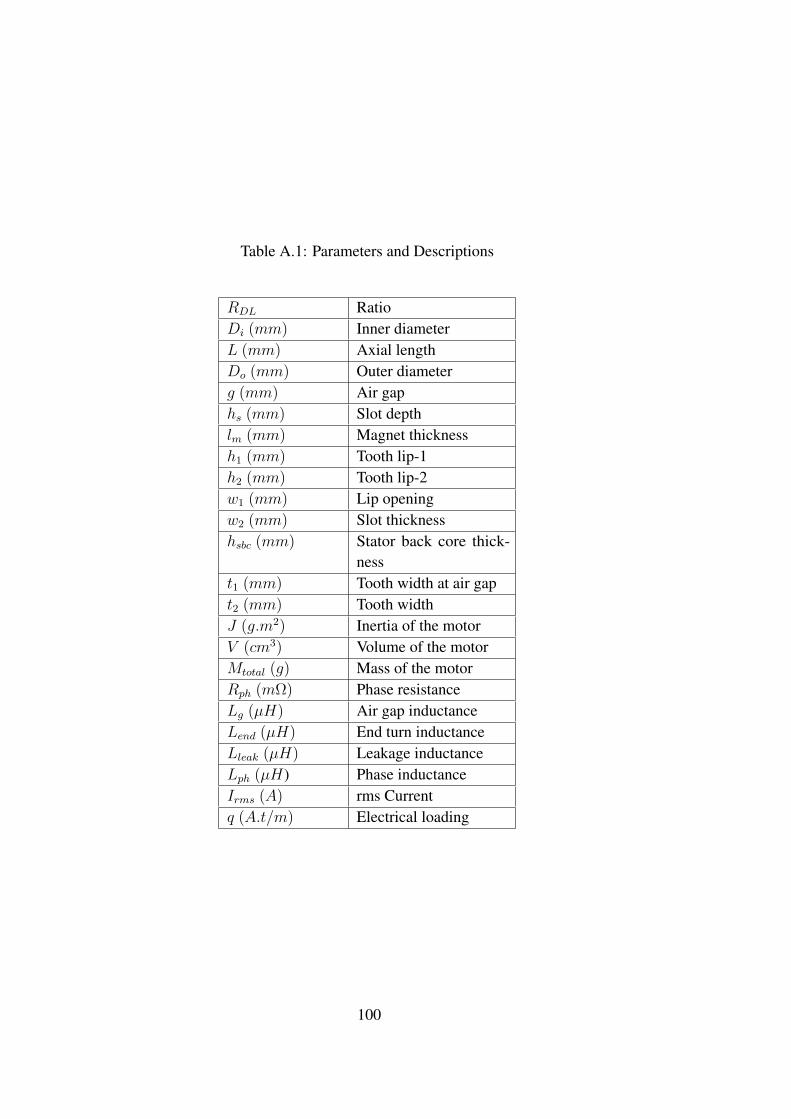
Table A.1: Parameters and Descriptions

RDL RatioDi (mm) Inner diameterL (mm) Axial lengthDo (mm) Outer diameterg (mm) Air gaphs (mm) Slot depthlm (mm) Magnet thicknessh1 (mm) Tooth lip-1h2 (mm) Tooth lip-2w1 (mm) Lip openingw2 (mm) Slot thicknesshsbc (mm) Stator back core thick-

nesst1 (mm) Tooth width at air gapt2 (mm) Tooth widthJ (g.m2) Inertia of the motorV (cm3) Volume of the motorMtotal (g) Mass of the motorRph (mΩ) Phase resistanceLg (µH) Air gap inductanceLend (µH) End turn inductanceLleak (µH) Leakage inductanceLph (µH) Phase inductanceIrms (A) rms Currentq (A.t/m) Electrical loading

100

APPENDIX B

DESIGN OUTPUTS WITH VARYING RATIO VALUES

This part shows the tabulated results upon applying the analytical solution with varying

ratio, in MATLAB. Sinusoidal 2-pole results are shown in Table B.1.

Sinusoidal 6-pole results are shown in Table B.2.

Squarewave 2-pole results are shown in Table B.3.

Squarewave 6-pole results are shown in Table B.4.

101

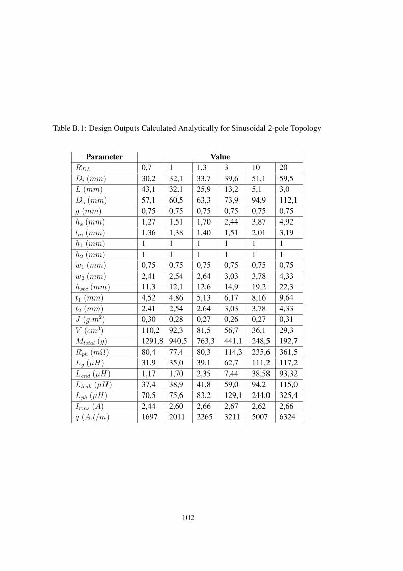
Table B.1: Design Outputs Calculated Analytically for Sinusoidal 2-pole Topology

Parameter ValueRDL 0,7 1 1,3 3 10 20Di (mm) 30,2 32,1 33,7 39,6 51,1 59,5L (mm) 43,1 32,1 25,9 13,2 5,1 3,0Do (mm) 57,1 60,5 63,3 73,9 94,9 112,1g (mm) 0,75 0,75 0,75 0,75 0,75 0,75hs (mm) 1,27 1,51 1,70 2,44 3,87 4,92lm (mm) 1,36 1,38 1,40 1,51 2,01 3,19h1 (mm) 1 1 1 1 1 1h2 (mm) 1 1 1 1 1 1w1 (mm) 0,75 0,75 0,75 0,75 0,75 0,75w2 (mm) 2,41 2,54 2,64 3,03 3,78 4,33hsbc (mm) 11,3 12,1 12,6 14,9 19,2 22,3t1 (mm) 4,52 4,86 5,13 6,17 8,16 9,64t2 (mm) 2,41 2,54 2,64 3,03 3,78 4,33J (g.m2) 0,30 0,28 0,27 0,26 0,27 0,31V (cm3) 110,2 92,3 81,5 56,7 36,1 29,3Mtotal (g) 1291,8 940,5 763,3 441,1 248,5 192,7Rph (mΩ) 80,4 77,4 80,3 114,3 235,6 361,5Lg (µH) 31,9 35,0 39,1 62,7 111,2 117,2Lend (µH) 1,17 1,70 2,35 7,44 38,58 93,32Lleak (µH) 37,4 38,9 41,8 59,0 94,2 115,0Lph (µH) 70,5 75,6 83,2 129,1 244,0 325,4Irms (A) 2,44 2,60 2,66 2,67 2,62 2,66q (A.t/m) 1697 2011 2265 3211 5007 6324

102

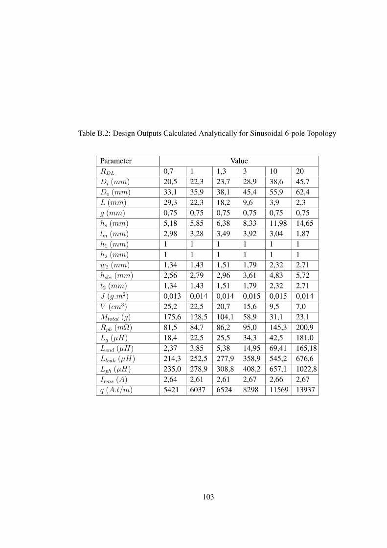
Table B.2: Design Outputs Calculated Analytically for Sinusoidal 6-pole Topology

Parameter ValueRDL 0,7 1 1,3 3 10 20Di (mm) 20,5 22,3 23,7 28,9 38,6 45,7Do (mm) 33,1 35,9 38,1 45,4 55,9 62,4L (mm) 29,3 22,3 18,2 9,6 3,9 2,3g (mm) 0,75 0,75 0,75 0,75 0,75 0,75hs (mm) 5,18 5,85 6,38 8,33 11,98 14,65lm (mm) 2,98 3,28 3,49 3,92 3,04 1,87h1 (mm) 1 1 1 1 1 1h2 (mm) 1 1 1 1 1 1w2 (mm) 1,34 1,43 1,51 1,79 2,32 2,71hsbc (mm) 2,56 2,79 2,96 3,61 4,83 5,72t2 (mm) 1,34 1,43 1,51 1,79 2,32 2,71J (g.m2) 0,013 0,014 0,014 0,015 0,015 0,014V (cm3) 25,2 22,5 20,7 15,6 9,5 7,0Mtotal (g) 175,6 128,5 104,1 58,9 31,1 23,1Rph (mΩ) 81,5 84,7 86,2 95,0 145,3 200,9Lg (µH) 18,4 22,5 25,5 34,3 42,5 181,0Lend (µH) 2,37 3,85 5,38 14,95 69,41 165,18Lleak (µH) 214,3 252,5 277,9 358,9 545,2 676,6Lph (µH) 235,0 278,9 308,8 408,2 657,1 1022,8Irms (A) 2,64 2,61 2,61 2,67 2,66 2,67q (A.t/m) 5421 6037 6524 8298 11569 13937

103

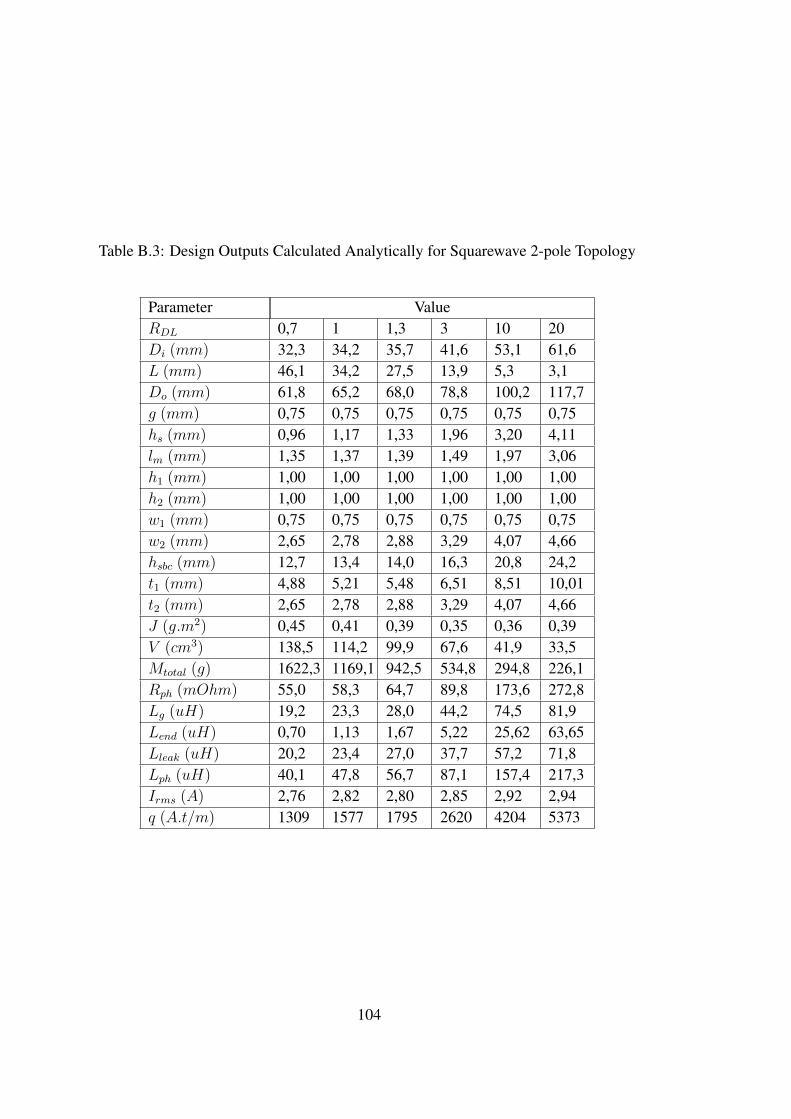
Table B.3: Design Outputs Calculated Analytically for Squarewave 2-pole Topology

Parameter ValueRDL 0,7 1 1,3 3 10 20Di (mm) 32,3 34,2 35,7 41,6 53,1 61,6L (mm) 46,1 34,2 27,5 13,9 5,3 3,1Do (mm) 61,8 65,2 68,0 78,8 100,2 117,7g (mm) 0,75 0,75 0,75 0,75 0,75 0,75hs (mm) 0,96 1,17 1,33 1,96 3,20 4,11lm (mm) 1,35 1,37 1,39 1,49 1,97 3,06h1 (mm) 1,00 1,00 1,00 1,00 1,00 1,00h2 (mm) 1,00 1,00 1,00 1,00 1,00 1,00w1 (mm) 0,75 0,75 0,75 0,75 0,75 0,75w2 (mm) 2,65 2,78 2,88 3,29 4,07 4,66hsbc (mm) 12,7 13,4 14,0 16,3 20,8 24,2t1 (mm) 4,88 5,21 5,48 6,51 8,51 10,01t2 (mm) 2,65 2,78 2,88 3,29 4,07 4,66J (g.m2) 0,45 0,41 0,39 0,35 0,36 0,39V (cm3) 138,5 114,2 99,9 67,6 41,9 33,5Mtotal (g) 1622,3 1169,1 942,5 534,8 294,8 226,1Rph (mOhm) 55,0 58,3 64,7 89,8 173,6 272,8Lg (uH) 19,2 23,3 28,0 44,2 74,5 81,9Lend (uH) 0,70 1,13 1,67 5,22 25,62 63,65Lleak (uH) 20,2 23,4 27,0 37,7 57,2 71,8Lph (uH) 40,1 47,8 56,7 87,1 157,4 217,3Irms (A) 2,76 2,82 2,80 2,85 2,92 2,94q (A.t/m) 1309 1577 1795 2620 4204 5373

104

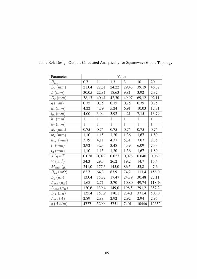
Table B.4: Design Outputs Calculated Analytically for Squarewave 6-pole Topology

Parameter ValueRDL 0,7 1 1,3 3 10 20Di (mm) 21,04 22,81 24,22 29,43 39,19 46,32L (mm) 30,05 22,81 18,63 9,81 3,92 2,32Do (mm) 38,13 40,41 42,30 49,97 69,12 92,11g (mm) 0,75 0,75 0,75 0,75 0,75 0,75hs (mm) 4,22 4,79 5,24 6,91 10,03 12,31lm (mm) 4,00 3,94 3,92 4,21 7,15 13,79h1 (mm) 1 1 1 1 1 1h2 (mm) 1 1 1 1 1 1w1 (mm) 0,75 0,75 0,75 0,75 0,75 0,75w2 (mm) 1,10 1,15 1,20 1,36 1,67 1,89hsbc (mm) 3,79 4,11 4,37 5,31 7,07 8,35t1 (mm) 2,92 3,23 3,48 4,39 6,09 7,33t2 (mm) 1,10 1,15 1,20 1,36 1,67 1,89J (g.m2) 0,028 0,027 0,027 0,028 0,040 0,069V (cm3) 34,3 29,3 26,2 19,2 14,7 15,4Mtotal (g) 241,0 177,3 145,0 86,5 53,8 47,6Rph (mΩ) 62,7 64,3 63,9 74,2 113,4 158,0Lg (µH) 13,04 15,82 17,47 24,79 30,48 27,11Lend (µH) 1,68 2,71 3,70 10,80 49,74 118,70Lleak (µH) 120,6 139,4 149,0 198,5 291,2 357,2Lph (µH) 135,4 157,9 170,1 234,1 371,4 503,0Irms (A) 2,89 2,88 2,92 2,92 2,94 2,95q (A.t/m) 4727 5299 5751 7401 10446 12652

105

106

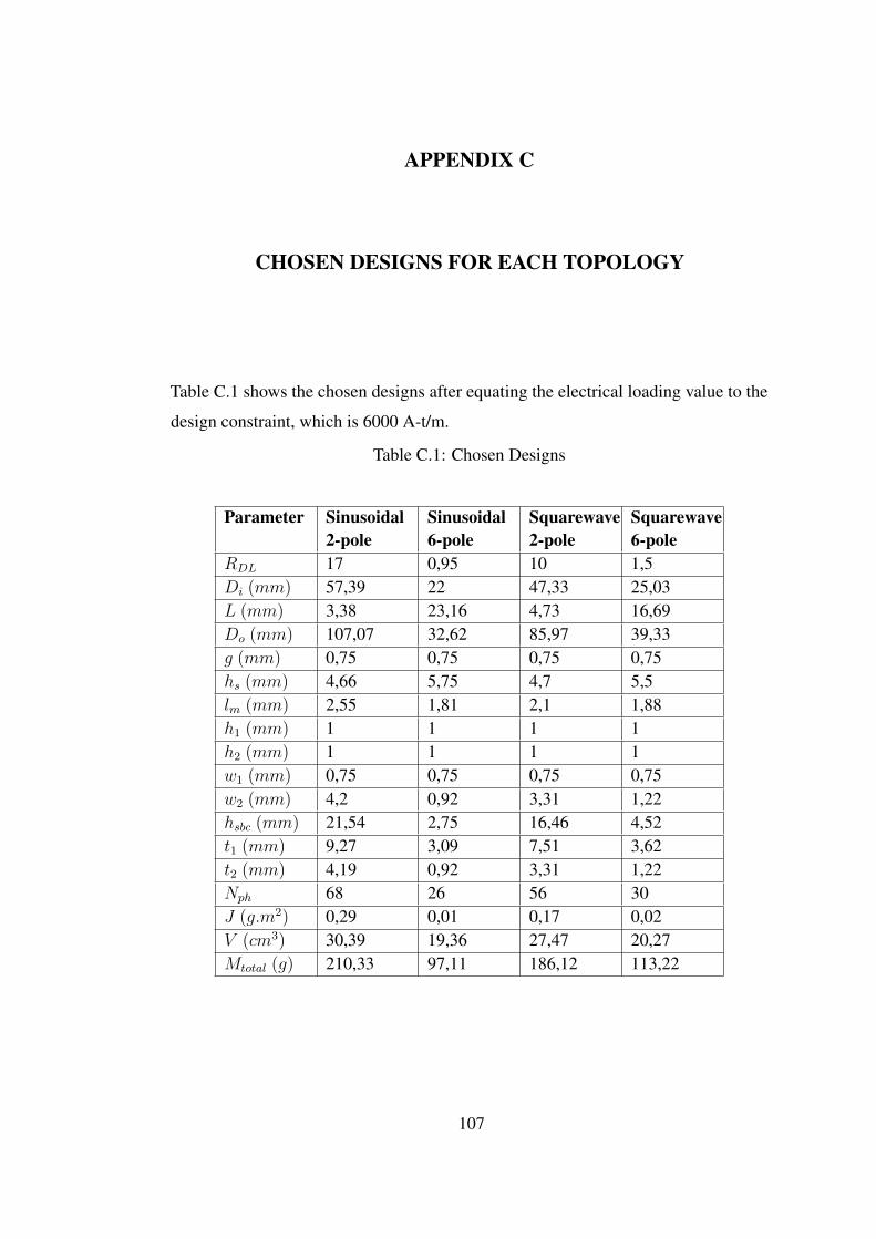
APPENDIX C

CHOSEN DESIGNS FOR EACH TOPOLOGY

Table C.1 shows the chosen designs after equating the electrical loading value to the

design constraint, which is 6000 A-t/m.

Table C.1: Chosen Designs

Parameter Sinusoidal2-pole

Sinusoidal6-pole

Squarewave2-pole

Squarewave6-pole

RDL 17 0,95 10 1,5Di (mm) 57,39 22 47,33 25,03L (mm) 3,38 23,16 4,73 16,69Do (mm) 107,07 32,62 85,97 39,33g (mm) 0,75 0,75 0,75 0,75hs (mm) 4,66 5,75 4,7 5,5lm (mm) 2,55 1,81 2,1 1,88h1 (mm) 1 1 1 1h2 (mm) 1 1 1 1w1 (mm) 0,75 0,75 0,75 0,75w2 (mm) 4,2 0,92 3,31 1,22hsbc (mm) 21,54 2,75 16,46 4,52t1 (mm) 9,27 3,09 7,51 3,62t2 (mm) 4,19 0,92 3,31 1,22Nph 68 26 56 30J (g.m2) 0,29 0,01 0,17 0,02V (cm3) 30,39 19,36 27,47 20,27Mtotal (g) 210,33 97,11 186,12 113,22

107

108

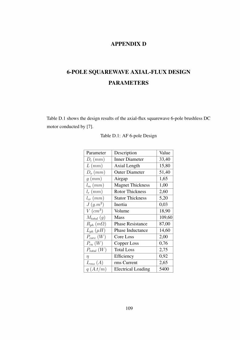
APPENDIX D

6-POLE SQUAREWAVE AXIAL-FLUX DESIGN

PARAMETERS

Table D.1 shows the design results of the axial-flux squarewave 6-pole brushless DC

motor conducted by [7].

Table D.1: AF 6-pole Design

Parameter Description ValueDi (mm) Inner Diameter 33,40L (mm) Axial Length 15,80Do (mm) Outer Diameter 51,40g (mm) Airgap 1,65lm (mm) Magnet Thickness 1,00lr (mm) Rotor Thickness 2,60lcr (mm) Stator Thickness 5,20J (g.m2) Inertia 0,03V (cm3) Volume 18,90Mtotal (g) Mass 109,60Rph (mΩ) Phase Resistance 87,00Lph (µH) Phase Inductance 14,60Pcore (W ) Core Loss 2,00Pcu (W ) Copper Loss 0,76Ptotal (W ) Total Loss 2,75η Efficiency 0,92Irms (A) rms Current 2,65q (A.t/m) Electrical Loading 5400

109