Embed Size (px)
Citation preview

Design of an eddy current damper for swing mode mitigation of the University of
Florida Torsion Pendulum
Undergraduate honors thesis
Brandon N. Bickerstaff
University of Florida
B.S. Mechanical Engineering
Summa Cum Laude
Spring 2017

Table of contents 1 Introduction .......................................................................................................................................... 1
1.1 Laser Interferometer Space Antenna [1] ...................................................................................... 1
1.2 University of Florida Torsion Pendulum [3] .................................................................................. 1
1.3 Motivation ..................................................................................................................................... 3
2 Engineering design process ................................................................................................................... 5
2.1 Identification of need .................................................................................................................... 5
2.2 Problem definition ........................................................................................................................ 5
2.3 Synthesis ....................................................................................................................................... 5
2.3.1 Bill of materials ..................................................................................................................... 6
2.3.2 Magnet case subassembly and corresponding assembly process ........................................ 6
2.3.3 ECD assembly and corresponding assembly process ............................................................ 8
2.3.4 Overview of parts ................................................................................................................ 11
2.4 Analysis and optimization ........................................................................................................... 19
2.4.1 Experimental setup ............................................................................................................. 19
2.4.2 Effect of gap distance .......................................................................................................... 19
2.4.3 Data summary ..................................................................................................................... 23
2.5 Evaluation ................................................................................................................................... 24
3 Conclusion ........................................................................................................................................... 25
4 Pictures ............................................................................................................................................... 26
5 References .......................................................................................................................................... 32

1
1 Introduction
1.1 Laser Interferometer Space Antenna [1] Although the use of electromagnetic radiation as a tool for extraterrestrial examination and discovery has
proven to be extremely powerful, to more comprehensively study and understand the universe, its
counterpart—gravity—must be more extensively perceived and employed as an investigative instrument.
Certainly, observing gravitational waves—ripples in the fabric of spacetime caused by some the most
violent and energetic processes in the universe [2] and gravity’s “messenger”—from cosmic sources will
allow otherwise inaccessible features of the universe to be explored.
In September of 2015, gravitational waves were identified for the first time by the two ground-based Laser
Interferometer Gravitational-Wave Observatory (LIGO) detectors—one in Livingston, Louisiana, and one
in Hanford, Washington. The undoubtedly groundbreaking discovery has since changed astronomy, as it
provided access to the high-frequency regime of gravitational waves—the realm of stellar mass objects at
low redshift and with relatively low mass. However, the low-frequency (below 1 Hz), relatively high-mass
realm—within which the heaviest and most diverse objects are expected to reside—will most likely not
be observable from the ground; rather, a space-based detector is needed.
Admittedly, the Laser Interferometer Space Antenna (LISA) is that needed space-based detector and will
allow further celestial exploration than currently possible via any alternative (e.g., LIGO). Associated with
a proposed launch year of 2030, it will provide a comprehensive view of the galaxy, using gravitational
waves as the advanced messengers, and subsequently disclose current scientific unknowns (e.g., the
histories of select black holes) related to outer space. Indeed, it will be the pioneer in gravitational wave-
based examinations of the universe and put Albert Einstein’s general theory of relativity to the test; it will
scan the entire sky, orbiting behind Earth and simultaneously acquiring both polarizations of gravitational
waves, and evaluate astrophysically relevant occurrences in a band from below 10-4 Hz to above 10-1 Hz.
Laser interferometry between free-flying test masses (TMs)—each one being contained within a
gravitational reference sensor (GRS)—housed inside drag-free spacecraft will be the foundation of LISA.
Within each spacecraft, two TMs will freely fall, with each one serving as a geodesic reference end mirror
for a single arm of the interferometer. Based on local interferometric position readouts, the spacecraft
will be forced to follow the TMs along the interferometric axes they respectively define (one each). Then,
the TMs will be electrostatically suspended to their corresponding spacecraft along the other degrees of
freedom, as both interferometric and capacitive position readouts control the dynamics. Finally, three
arms with six active laser links shared among three identical spacecraft in an equilateral triangular
formation with edge lengths of 2.5 Gm will constitute the layout of the observatory.
1.2 University of Florida Torsion Pendulum [3] At the University of Florida (UF), a unique torsion pendulum—the UF Torsion Pendulum—has been, and
continues to be, developed to test new technologies for the LISA GRS (described in Section 1.1), with
quantifying the acceleration noise performance of ultra-precise inertial sensors (i.e., GRSs) being the
primary focus of the corresponding research and development. The apparatus consists of a 1-meter-long,
50-micrometer-diameter, tungsten fiber that is enclosed in a vacuum chamber and supports an aluminum
crossbar with one hollow cubic TM at each of its four ends, allowing the rotation of the torsion pendulum
to be converted into translation of the TMs. Two opposing TMs are enclosed in capacitive sensors which
provide both position readout and actuation, and these test masses are electrically insulated from the

2
rest of the system and have their electrical charges controlled via photoemission using fiber-coupled
ultraviolet light-emitting diodes. Although the capacitive readout can accurately measure the TMs’
displacements, it is complemented by a more accurate laser interferometer.
Additionally, the system is equipped with various rotational and translational positioning stages used to
accurately align the pendulum with the sensors, as well as conductive shields that prevent electrostatic
interactions between the inertial member (i.e., the pendulum) and charges that may accumulate on
dielectric surfaces—e.g., the surfaces of the cables, windows, and other non-metallic parts. At the top of
the chamber, a relatively thick tungsten fiber is suspended; that fiber is connected to a threaded rod (the
transition rod) to which a conducting disc is fastened; then, the relatively thin tungsten fiber is linked to
the bottom of the aforementioned threaded rod, and the pendulum is mounted at the bottom of the
latter fiber (via a 10-centimeter-long shaft). The conducting disc passes through an inhomogeneous
magnetic field created by neodymium magnet arrays contained in cases adjacent to and above and below
the disc; the cases are suspended via three threaded rods (the suspension rods) that fasten into the
vacuum flange at the top of the chamber. When swinging, the two fibers behave like a single, longer fiber,
and the disc moves with respect to the magnetic field. Consequently, eddy currents are generated within
the disc and the kinetic swing-mode energy of the dynamic pendulum is dissipated as heat (due to the
disc having a non-zero resistivity). Therefore, the latter disc–magnetic field setup is referred to as the eddy
current damper (ECD) and mitigates the swing mode of the pendulum. Note that the previously explained
components are shown in Figure 1.
3
Figure 1: The above figure depicts an overview of the UF Torsion Pendulum. The ECD—the second
component from the top—is the primary focus of the research and development subsequently presented
in this report. It is suspended via three threaded suspension rods that fasten into tapped holes in the
vacuum flange at the top of the chamber. Also, threaded fiber caps are used for the vacuum flange-to-
thick fiber, thick fiber-to-transition rod, transition rod-to-thin fiber, and thin fiber-to-pendulum shaft
connections. (Note that the turbo pump is used to achieve a near-vacuum state within the chamber.)
1.3 Motivation Admittedly, the original ECD serves as the basis of the subsequent design. It uses two magnet-filled cases,
with central clearance holes, suspended via three threaded suspension rods (that run through clearance
holes in the cases) and held in place via nuts threaded onto both ends of the latter rods until they coincide
with the corresponding annular surfaces of the cases; i.e., three nuts (one corresponding to each
suspension rod) coincide with both the top and bottom of each case. The cases surround a conducting
disc with a central clearance hole; the transition rod runs through the latter clearance hole, and the disc
is held in place via nuts threaded onto both ends of the latter rod until they coincide with corresponding
annular surfaces of the disc.
However, the original ECD does not effectively damp the kinetic swing-mode energy of the pendulum,
resulting in dynamic range issues and nonlinear coupling in the readout related to the rotational motion
14-centimeter-long, 250-micrometer-diameter, tungsten fiber
ECD
Rotational and translational manipulators
Turbo pump
Electrostatic shields TM inside simplified GRS
10-centimeter-long shaft
1-meter-long, 50-micrometer-diameter, tungsten fiber
4
of the pendulum. First of all, the magnets are not optimally positioned, resulting in a magnetic field that
is weaker than desired within the disc’s range of motion and, subsequently, minimal damping.
Additionally, due to the nuts present between cases, the cases cannot be positioned as closely as desired,
also resulting in minimal damping (via the mechanism described in the second paragraph of Section 1.2).
Similarly, due to the nuts present between cases and coinciding with each annular surface of the disc, as
well as the suspension rods running through the cases, the disc is geometrically constrained and prone to
getting “stuck,” resulting in difficulty properly aligning the pendulum with the rotational and translational
manipulators. Therefore, due to the strict noise requirements that need to be met, an improved and highly
effective ECD—one that satisfies the need and meets the specs outlined in Sections 2.1 and 2.2,
respectively—is desired.

5
2 Engineering design process
2.1 Identification of need There is a need for an ECD that
effectively mitigates the swing mode of the UF Torsion Pendulum;
allows for interference-free, reasonable swing motion to occur;
is vacuum-compatible;
consists of non-magnetic suspended (i.e., non-fixed) parts;
fits inside and fastens near the top of the vacuum chamber;
and is more strictly toleranced.
2.2 Problem definition The design specs are as follows:
1. Reuse the
a. three tapped holes into which the suspension rods fasten,
b. thick and thin fibers,
c. fiber caps,
d. transition rod, and
e. magnets.
2. Design such that the maximum OD (outer diameter) of the ECD is less than 2.245 in. (57.02 mm);
i.e., design for a minimum of 1/16 in. of clearance—between the ECD’s OD and the cylindrical
housing’s ID (inner diameter)—all the way around the ECD.
3. Allow for gap adjustability.
4. Prevent the conducting disc from getting “stuck.”
5. Provide 3 mm (nominally) of clearance all the way around the ODs of both the transition rod and
conducting disc.
6. Force the oscillation to half of its original amplitude in 3 min (order of magnitude).
2.3 Synthesis After about ten iterations through the synthesis, analysis and optimization, and evaluation steps of the
engineering design process, the concept presented in the following subsections was ultimately selected.
Without a doubt, the most challenging aspects of the design were maximizing the number of magnets
while meeting the overall size requirement (spec 2) and allowing for gap adjustability (spec 3). The layout
of the magnets was changed numerous times, and the selected concept uses six more magnets than the
original ECD does, with all the magnets being more optimally positioned. Additionally, using flat washers
to vary the distance between the magnet cases was considered, but using slotted rails was ultimately
chosen (as shown and discussed in Figure 6.)
6
2.3.1 Bill of materials Table 1: The following table presents the bill of materials (BOM) related to the ECD.
Part number Part name Details (if applicable) Material Quantity
1 Magnet tray — Aluminum 2
2 Magnet — Neodymium 30
3 Magnet cover — Aluminum 2
4 Pan head screw 2-56 x 1/4" Brass 6
5 Conducting disc — Aluminum 1
6 Transition rod 10-32 external threads Brass 1
7 Rail — Aluminum 3
8 Flat washer 4-40 (clearance), 0.040" thick Stainless steel 6
9 Hex head screw 4-40 x 1/4" Stainless steel 9
10 Adapter — Aluminum 3
11 Suspension rod 10-32 external threads Low-strength steel 3
12 Hex nut 10-32 (tapped), 1/8" thick Brass 6
13 Thick fiber — Tungsten 1
14 Fiber cap — Aluminum 3
15 Top mounting rod 10-32 external threads Brass 1
2.3.2 Magnet case subassembly and corresponding assembly process
Figure 2: The above figure shows the front (in the upper left), bottom (in the bottom left), right cross-
sectional (in the upper right), and isometric (in the bottom right) views of the magnet case subassembly.
There are two magnet cases in the ECD assembly—one above the conducting disc and one below it.

7
Figure 3: The above figure shows the exploded view of the magnet case subassembly, including part-
number balloons and leaders that reference the BOM provided in Table 1. Each of the two magnet cases
consists of fifteen magnets, arranged in a symmetrical manner about the central axis; one magnet cover;
and three pan head screws. The screws go through their corresponding clearance holes in the cover and
fasten into their corresponding thru-tapped holes in the tray, consequently fastening the cover to the tray
and holding the magnets in place. Note that the magnet holes are slightly larger in diameter than the
magnets and have thin-walled features remaining at their bottoms to securely seat the magnets, as shown
by the cross-sectional view in Figure 2.
1
2
3
4

8
2.3.3 ECD assembly and corresponding assembly process
Figure 4: The above figure shows the front (on the left) and right-side (on the right) views of the ECD
assembly, which consists of two magnet case subassemblies (shown in Figure 2) and numerous hex head
screws, flat washers, hex nuts, threaded rods, etc. Note that the overall BOM is provided in Table 1.

9
Figure 5: The above figure shows an isometric view of the ECD assembly, which consists of two magnet
case subassemblies (shown in Figure 2) and numerous hex head screws, flat washers, hex nuts, threaded
rods, etc. Note that the overall BOM is provided in Table 1.

10
Figure 6: The above figure shows the exploded view of the ECD assembly, including part-number balloons
and leaders that reference the BOM provided in Table 1. Additionally, the rectangular text box and
corresponding leader denotes the magnet case subassembly shown and discussed in Figure 3. To
assemble the ECD, hex head screws are inserted through the flat washers and subsequently through the
clearance slot in the rails. With the conducting disc “sandwiched” between the two magnet cases, the hex
head screws are then fastened into their respective magnet cases. Next, the transition rod is threaded
through the conducting disc, a fiber cap is threaded onto the bottom end of the transition rod, and the
additional hex head fasteners are used to fasten the adapters onto the rails. The suspension rods are then
inserted through the top clearance holes in the adapters and held in place via hex nuts tightened both
above and below the flange features of the adapters. Finally, after carefully adhering the two fiber caps
to the thick fiber—one on each end—the one on the bottom end is fastened onto the transition rod,
whereas the one on the other/top end is fastened onto the top mounting rod.
6 9
7 10
8
11
13
14
12
15
5
Magnet case

11
2.3.4 Overview of parts In the following figures, the parts constituting the ECD assembly are shown, and their materials,
quantities, functions, mates, etc. are discussed in the corresponding captions. The figures are ordered in
the same manner as the BOM (Table 1). Also, note that all the parts—excluding the rails, adapters, flat
washers, and hex head screws—were present in the original ECD, although some of those original parts
were modified and, thus, remanufactured. Therefore, in the new (and improved) ECD, the same materials
are used for the parts related to the original ones, as some parts (e.g., the thick fiber and fibers caps) were
reused, and it is desired to maintain some similarity between the original and new ECDs. Additionally, the
magnet trays, magnet covers, and conducting disc were originally aluminum (and are aluminum in the
new ECD). Due to its high machinability, aluminum is used for the rails and adapters. Furthermore,
stainless steel is used for the hex head screws and flat washers, as McMaster-Carr does not carry brass
hex head screws of the needed dimensions, and is it desired for the washers to be harder than brass.
Figure 7: The above figure displays an aluminum magnet tray; there are two of them in the ECD assembly.
Its function is to house the magnets, and each tray can hold fifteen. The magnet holes are slightly larger
in diameter than the magnets themselves (close-fit clearance), and a small (about 0.5 mm thick) flange
resides at their bottoms to seat the magnets. The machining of such a thin flange is made possible by thru
drilling out most the corresponding hole before plunging with an endmill, hence why the magnet holes
do not simply have flat, uniform bases. There are three 2-56 thru-tapped holes on the top surface of the
tray into which the pan head screws fasten to secure the magnet cover. The thickness of the tray is less
than the height of the magnets, which ensures that the magnets will be properly seated / prevents axial
translation of the magnets when the cover is assembled onto the tray. Additionally, there are three 4-40
blind-tapped holes on the circumferential surface of the tray into which hex head screws fasten to secure
the magnet cases (discussed/shown in Section 2.3.2) on the rails. Note that clearance hole through its
center in the center allows for the fiber and conducting disc to translate freely.

12
Figure 8: The above figure displays a neodymium (grade N52) magnet; there are thirty of them in the ECD
assembly. The function of the magnets is to generate an inhomogeneous magnetic field between the two
magnet cases, with the magnets dispersed as in Figure 3. The diameter and height of each cylindrical
magnet are both 1/4 in.
Figure 9: The above figure displays an aluminum magnet cover; there are two of them in the ECD
assembly. Its function is to secure the magnets in the magnet tray, prohibiting them from falling out. There
are three 2-56 close-fit clearance holes on the annular surfaces of the cover through which the pan head
screws freely go before fastening into their respective threaded holes in the magnet tray.
13
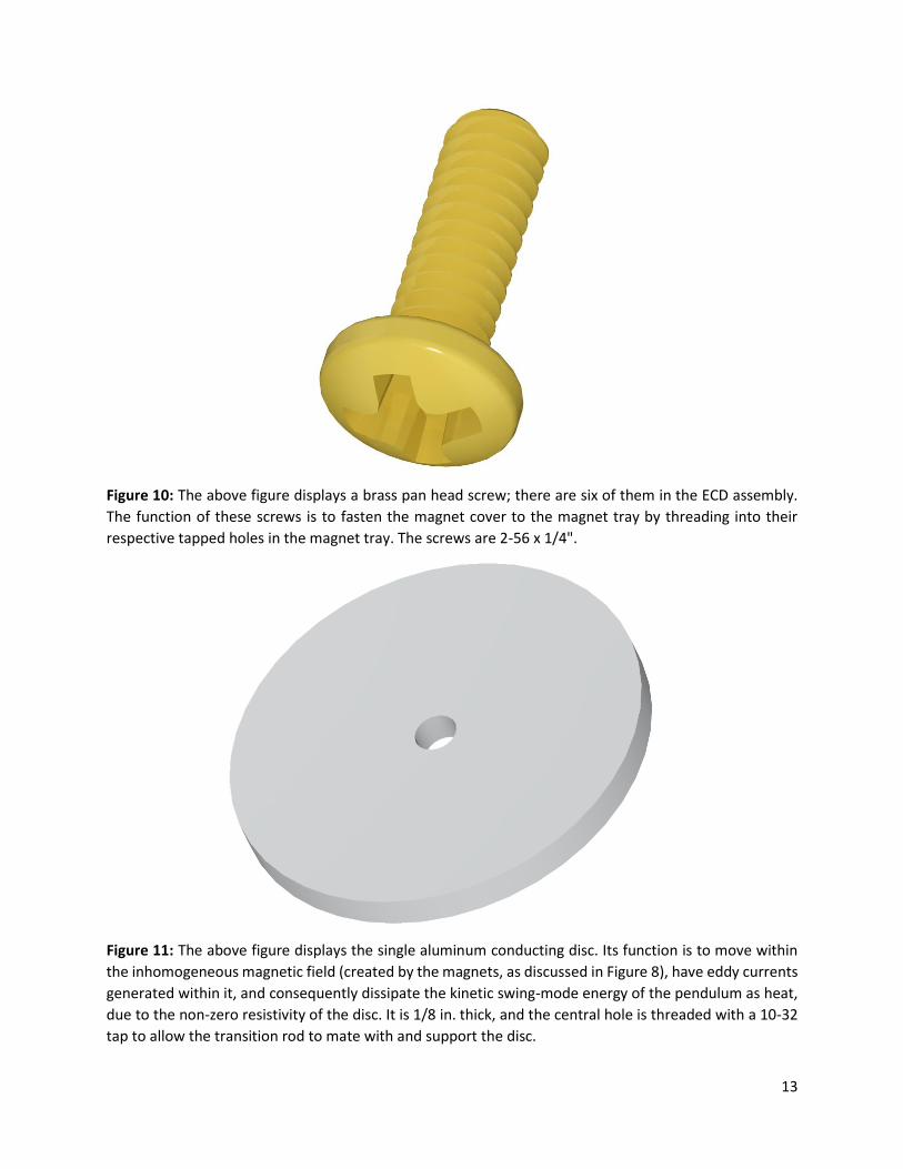
Figure 10: The above figure displays a brass pan head screw; there are six of them in the ECD assembly.
The function of these screws is to fasten the magnet cover to the magnet tray by threading into their
respective tapped holes in the magnet tray. The screws are 2-56 x 1/4".
Figure 11: The above figure displays the single aluminum conducting disc. Its function is to move within
the inhomogeneous magnetic field (created by the magnets, as discussed in Figure 8), have eddy currents
generated within it, and consequently dissipate the kinetic swing-mode energy of the pendulum as heat,
due to the non-zero resistivity of the disc. It is 1/8 in. thick, and the central hole is threaded with a 10-32
tap to allow the transition rod to mate with and support the disc.

14
Figure 12: The above figure displays the single brass transition rod. Its function is to provide the interface
between the interface and “transition” between the upper, thick fiber and the lower, thin fiber, while
supporting (i.e., threading into) the conducting disc. It is 2 in. long and has 10-32 external threads.
Figure 13: The above figure displays an aluminum rail; there are three of them in the ECD assembly. The
function of the rails is to hold the magnet cases while allowing them to be vertically adjustable. There is a
4-40 thru-tapped hole in the upper, cubic portion of the rail into which a hex head screw fastens (to mate
the rail with its corresponding adapter), and the vertical clearance slot is specifically sized for the 4-40 hex
head screws, allowing vertical adjustability of the magnet cases into which they fasten.

15
Figure 14: The above figure displays a stainless-steel flat washer; there are six of them in the ECD
assembly. The functions of the washers are to account for the possibility of the blind-tapped holes in the
magnet tray not being drilled and/or tapped deep enough and prevent damages to the rails by more
uniformly distributing the fastening contact stresses and protecting them from scarring via the screw
heads. Through the centers of the washers, free-fit clearance holes for 4-40 hex head screws are present.
Figure 15: The above figure displays a stainless-steel hex head screw; there are nine of them in the ECD
assembly. The function of these screws is to fasten both the magnet cases and adapters to the rails by
threading into their respective tapped holes in the magnet trays and rails. The screws are 4-40 x 1/4".

16
Figure 16: The above figure displays an aluminum adapter; there are three of them in the ECD assembly.
Its function is to provide the interface between a suspension rod and its corresponding rail. There is a 4-
40 close-fit clearance hole through the bottom of the part to allow a hex head screw to slide through
before mating with its corresponding rail. Additionally, there is a 10-32 close-fit clearance hole through
the upper flange to allow a suspension rod to slide through before being secured by hex nuts.
Figure 17: The above figure displays a low-strength-steel suspension rod. The function of these rods is to
support the adapter–rail–case assembly by passing through the upper flanges of the adapters and being
secured, above and below the flange, by hex nuts. It is about 5.7 in. long and has 10-32 external threads.

17
Figure 18: The above figure displays a brass hex nut; there are six of them in the ECD assembly. The
function of the nuts is to secure the suspensions rods to the adapter by threading onto each, both above
and below the upper flange of the corresponding adapter, tightly. The nuts have 10-32 internal threads.
Figure 19: The above figure displays the single tungsten thick fiber. Its function is to suspend the
conducting disc, as it is adhered to the upper fiber cap (that is fastened to the top mounting rod, which is
threaded into the vacuum flange at the top of the chamber), as well as the fiber cap on top of the transition
rod, and, thus, connected to the transition rod that supports the disc. It is about 16 cm long and has a
diameter of 250 μm.

18
Figure 20: The above figure displays an aluminum fiber cap and its cross section (internal threads not
shown); there are three of them in the ECD assembly. The function of the caps is to fasten onto the brass
rods and provide connection points for the tungsten fibers. With respect to the figure, at the bottom of
each cap, a 10-32 blind-tapped hole is present (for rod connection), whereas, at the top of each cap, a
0.028" (#70) thru hole is present (for fiber connection), as shown by the cross-sectional view. (When the
caps are incorporated into the UF Torsion Pendulum, smaller clearance holes will be used.)
Figure 21: The above figure displays the single brass top mounting rod. Its function is to provide the
interface between the top of the vacuum chamber / mounting point and the upper fiber cap which “holds”
the thick fiber. It is 0.5 in. long and has 10-32 external threads.

19
2.4 Analysis and optimization An experiment was set up to evaluate the performance of the new ECD, synthesized in Section 2.3. The
goal of the experiment was to measure the oscillatory behavior of a pendulum related to three different
ECD gap distances—where the gap distance is the distance between the inner surfaces of the magnet
cases—and the goal of the subsequent data analysis (presented in the following subsections) is to study
the acquired data and quantify the effectiveness of the ECD. Related to the former, the position of a
reference mass was measured by a data acquisition (DAQ) system that used a non-contact position sensor,
and each positional data point was timestamped using a computer program; and, related to the latter,
using spreadsheets and computational software, the data are processed to calcluate the average half-
amplitude decay time and additional statistics corresponding to each scenario, tabulated to determine
the most effective gap distance and predict the damping performance related to that scenario when the
ECD is incorporated into the UF Torsion Pendulum, and plotted to develop a functional relationship
between the decay time and gap distance.
2.4.1 Experimental setup The experiment was set up in a sturdy metal cabinet with two vertically adjustable shelves. The top shelf
had four thru holes machined in it that allow the three suspension rods and single top mounting ride to
slide through and be secured by 10-32 hex nuts on their upper ends. A fiber cap was mechanically affixed
to each end of a 1-meter-long, vertical copper wire; the top cap was fastened onto the bottom of the
transition rod, and the bottom cap was fastened onto a 10-32 stud that had a nut on one end and passed
through the clearnace hole in the center of a 0.45-kilogram, cylindrical “dummy” mass. For the purposes
of this experiment, the copper wire simulates the thin tungesten fiber, and the dummy mass simulates
the pendulum (including its weight), both of which are discussed in Section 1.2.
Furthermore, the bottom shelf was positioned just beneath the bottom surface of the suspended dummy
mass. The electronics used for DAQ—i.e., Raspberry Pi, breadboards, circuitry, and position sensor—were
mounted on the bottom shelf; and the monitor, keyboard, and mouse were connected to the Raspberry
Pi but located outside of the cabinet, which allowed the cabinet’s door to be closed during DAQ. (Acquiring
data with the door closed resulted in significanlty reduced unwanted oscillations, due to air currents, for
example.) The position sensor was set up to operate in its approximately linear region on the left-hand
side of the plot in the Engineering Data section of [4] related to “black paper” (which is adequate for the
purposes of this experiment); it was set up with its sensing direction normal to the cylindrical surface of
the dummy mass, outputs a signal that is (approximately) directly proportional to the distance between
the sensor and the near cylindrical surface of the dummy mass, and has an associated distance resolution
of about 25 μm. A Python program that captures the latter signal and its related timestamp at a sampling
frequency of 500 Hz, with the option to display and/or save (to .csv) those two values (at each program
iteration), was written and uploaded onto the Raspberry Pi, and the raw data were analyzed on an
external laptop using both Excel and MATLAB.
2.4.2 Effect of gap distance In this section, the effect gap distance has on the damping performance of the ECD is studied. Small,
intermediate, and large gaps distances of 5.62 mm, 9.97 mm, and 13.36 mm, respectively, were employed,
and each scenario is subsequently analyzed (in that order). For each setup, the north-pole vectors of all
the magnets were oriented in the same direction and data were acquired for two runs to generate more
representative statistics.

20
Figure 22: The above figure displays the oscillatory behavior of the dummy mass related to run 1 of the
small-gap distance scenario of 5.62 mm, shown in Table 2. The intentional impulse occurred at about the
10-second mark (shown on this figure only to depict the essentially consistent before-impulse behavior of
the dummy mass), and the amplitude associated with that impulse is about 5 mm. Because the sensor is
approximated as linear, to account for the signals not being “perfectly” symmetrically dispersed about the
average signal (which corresponds to the equilibrium positon of the dummy mass), the half-amplitude
decay time was determined for both the upper and lower profiles by determining the maximum and
minimum signals using Excel, calculating the corresponding half-amplitude signals using Excel, and probing
a MATLAB plot (of the same data displayed above) at its upper and lower profiles to find the times
associated with the previously calculated half-amplitude signals. For this run specifically, the average half-
amplitude decay time was calculated to be 138.5 s (2.3 min), and the sample standard deviation of the
half amplitude decay times was calculated to be 1.5 s.

21
Figure 23: The above figure displays the oscillatory behavior of the dummy mass related to run 1 of the
intermediate-gap distance scenario of 9.97 mm, shown in Table 2. The amplitude associated with the
intentional impulse (at the 0-second mark) is about 4.5 mm. Because the sensor is approximated as linear,
to account for the signals not being “perfectly” symmetrically dispersed about the average signal (which
corresponds to the equilibrium positon of the dummy mass), the half-amplitude decay time was
determined for both the upper and lower profiles by determining the maximum and minimum signals
using Excel, calculating the corresponding half-amplitude signals using Excel, and probing a MATLAB plot
(of the same data displayed above) at its upper and lower profiles to find the times associated with the
previously calculated half-amplitude signals. For this run specifically, the average half-amplitude decay
time was calculated to be 593.2 s (9.9 min), and the sample standard deviation of the half amplitude decay
times was calculated to be 7.9 s.
22
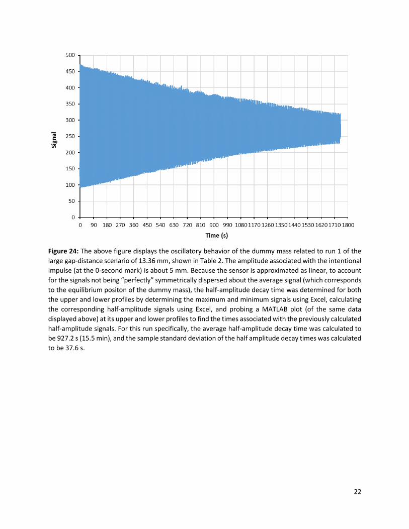
Figure 24: The above figure displays the oscillatory behavior of the dummy mass related to run 1 of the
large gap-distance scenario of 13.36 mm, shown in Table 2. The amplitude associated with the intentional
impulse (at the 0-second mark) is about 5 mm. Because the sensor is approximated as linear, to account
for the signals not being “perfectly” symmetrically dispersed about the average signal (which corresponds
to the equilibrium positon of the dummy mass), the half-amplitude decay time was determined for both
the upper and lower profiles by determining the maximum and minimum signals using Excel, calculating
the corresponding half-amplitude signals using Excel, and probing a MATLAB plot (of the same data
displayed above) at its upper and lower profiles to find the times associated with the previously calculated
half-amplitude signals. For this run specifically, the average half-amplitude decay time was calculated to
be 927.2 s (15.5 min), and the sample standard deviation of the half amplitude decay times was calculated
to be 37.6 s.

23
2.4.3 Data summary Table 2: Because the sensor is approximated as linear, to account for the signals not being “perfectly”
symmetrically dispersed about the average signal (which corresponds to the equilibrium positon of the
dummy mass), the half-amplitude decay time was determined for both the upper and lower profiles by
determining the maximum and minimum signals using Excel, calculating the corresponding half-amplitude
signals using Excel, and probing a MATLAB plot of the relevant data at its upper and lower profiles to find
the times associated with the previously calculated half-amplitude signals. Furthermore, for each
scenario, data were acquired for two runs to generate more representative statistics. Clearly, the small
gap distance of 5.62 mm resulted in the best/quickest damping and most precise results, as it had the
smallest associated standard deviation.
Gap Run Profile
Half-amplitude decay time
Average half-amplitude decay time
Standard deviation of half-amplitude
decay times
scenario distance (mm) (s) (min) (s) (min) (s) (min)
Small 5.62
1 Upper 139.6 2.3
134.6 2.2 4.9 0.1 Lower 137.5 2.3
2 Upper 128.6 2.1
Lower 132.6 2.2
Intermediate 9.97
1 Upper 598.8 10.0
603.2 10.1 13.2 0.2 Lower 587.7 9.8
2 Upper 607.6 10.1
Lower 618.7 10.3
Large 13.36
1 Upper 953.8 15.9
912.2 15.2 55.5 0.9 Lower 900.6 15.0
2 Upper 956.0 15.9
Lower 838.3 14.0

24
Figure 25: The above figure displays the relationship between the average half-amplitude decay time and
the gap distance by plotting the relevant values from Table 2. A linear trendline—given by the equation
𝑡 = 100.8𝑑 − 422.73, where 𝑡 is the average half-amplitude decay time and 𝑑 is the gap distance—was
fit to the three data points, and the associated coefficient of determination (𝑅2) is 0.9978. Thus, within
the gap distance domain from 5.62 mm to 13.36 mm, the latter equation can be used to predict 99.78%
of the variation in the average half-amplitude decay time based on the variation in the gap distance.
Vertical error bars corresponding to plus/minus one sample standard deviation are also shown but
difficult to see for the small-gap distance scenario.
2.5 Evaluation Based on the synthesis and analysis and optimization presented in Sections 2.3 and 2.4, respectively, the
need (presented in Section 2.1) was indeed satisfied, and the specs (presented in Section 2.2) were indeed
met. The designed ECD effectively damps the swing mode of the UF Torsion Pendulum; allows for
interference-free, reasonable swing motion to occur; is vacuum-compatible; consists of non-magnetic
suspended (i.e., non-fixed) parts; fits inside and fastens near the top of the vacuum chamber; and is more
strictly toleranced. Additionally, the designed ECD allows for the three tapped holes into which the
suspension rods fasten, thick and thin fibers, fiber caps, transition rod, and magnets to be reused; 1/16
in. of clearance is present between the ECD’s OD and the cylindrical housing’s ID, all the way around the
ECD, and 3 mm of clearance is nominally present all the way around the ODs of both the transition rod
and conducting disc; gap adjustability is allowed for (via the rails), and the disc cannot get “stuck” when
swinging between the magnet cases (due to the space between the interior surfaces of the magnet cases
being completely open); and the oscillation is forced to half of its original amplitude in less than 3 min—
in 2.2 ± 0.1 min, to be exact (for the small-gap distance scenario of 5.62 mm).
y = 100.8x - 422.73R² = 0.9978
0
100
200
300
400
500
600
700
800
900
1000
0 1 2 3 4 5 6 7 8 9 10 11 12 13 14
Ave
rage
hal
f-am
plit
ud
e d
eca
y ti
me
(s)
Gap distance (mm)

25
3 Conclusion In order to more comprehensively study and understand the universe, gravity must be better understood
and more frequently utilized. Although gravitational waves, the “messenger” of gravity, have been
detected within the high-frequency regime (by LIGO detectors), it is desired to detect them within the
low-frequency realm, as that is where the heaviest and most diverse objects are expected to reside [1].
Indeed, it will most likely only be possible to observe gravitational waves within the latter realm using a
space-based detector such as LISA. LISA will be capable of measuring astrophysically relevant occurrences
in a band from below 10-4 Hz to above 10-1 Hz by employing laser interferometry between free-flying TMs
housed within GRSs inside three identical spacecraft in an equilateral triangular formation with edge
lengths of 2.5 Gm [1].
At UF, a unique torsion pendulum has been continually developed for several years to test new
technologies for the LISA GRS, and the primary focus of the corresponding research and development has
been, and continues to be, quantifying the acceleration noise performance of ultra-precise inertial
sensors—the GRSs [3]. The apparatus consists of an aluminum crossbar with one hollow cubic TM at each
of its four ends suspended in a vacuum chamber such that the rotation of the torsion pendulum is
converted into translation of the TMs [3]. Capacitive sensors used (partly) for position readout enclose
two opposing test masses and measure the rotational displacement of the pendulum / translation of the
TMs [3]. However, when the swing mode of the pendulum is excessively disturbed, issues regarding
dynamic range and nonlinear coupling in the rotational readout arise. To mitigate the swing mode, an ECD
is used, consisting of an inhomogeneous magnetic field and a conducting disc (that is connected to the
pendulum’s suspension fiber via a fiber cap and threaded rod). As the pendulum swings, eddy currents
are generated within the disc, and the kinetic swing-mode energy of the dynamic pendulum is dissipated
as heat (due to the disc having a non-zero resistivity) [3].
Admittedly, the original ECD does not effectively damp the pendulum’s swing mode, due primarily to
geometric constraints. Consequently, it was desired to design an improved and highly effective ECD, and
that design process was presented in Section 2. At the end of the latter process, it was both qualitatively
and quantitatively shown that the need was satisfied and the specs were met. The designed ECD allows
for 3 mm of interference-free swing motion of the conducting disc to occur (horizontally/radially), which
translates to over 25 mm of interference-free swing motion of the pendulum—significantly more than
what occurs in practice; it also allows for gap adjustability and forces the swing oscillation to half of its
original amplitude in 2.2 ± 0.1 min (related to the optimal setup).
Although the modularity of the designed ECD proved to be helpful for frequent assembly/disassembly
(which was required for empirical testing purposes), it would be advantageous for structural and long-
term-use reasons to make the rail and adapter a single part. Furthermore, because manual assembly is
required, it would be worthwhile to determine whether larger fasteners could be used. Similarly, it would
be helpful to have variable-thickness shims made or incorporate geometric support features into the
design itself to assist in resisting the strong attraction/repulsion between the magnet cases during
assembly/disassembly. Lastly, on the experimental front, it is recommended that data be acquired for
more gap-distance scenarios, and for more runs related to each gap-distance scenario, to obtain more
accurate results and a more representative damping time vs. gap distance plot (Figure 25). It is also
suggested that various magnet polarity configurations be tested to determine which is the most effective
at damping the swing mode.

26
4 Pictures On the five following pages, pictures of the assembled ECD and experimental setup are shown.

27
Figure 26: The above picture shows the full view of the assembled ECD mounted in the cabinet. The copper
wire at the bottom is attached to the dummy mass (shown in Figure 28). Refer to Figure 6 and its
associated references for details about the individual components, assembly, etc.
Copper wire
Shelf

28
Figure 27: The above picture shows the zoomed view of the assembled ECD mounted in the cabinet. The
copper wire at the bottom is attached to the dummy mass (shown in Figure 28). Refer to Figure 6 and its
associated references for details about the individual components, assembly, etc.
Copper wire

29
Figure 28: The above picture shows the experimental setup. Refer to Section 2.4.1 for details.
Copper
wire
ECD
Shelf
Dummy
mass
DAQ
system

30
Figure 29: The above picture shows the DAQ system and dummy mass. Refer to Section 2.4.1 for details.
Raspberry Pi
Breadboards
and circuitry
Dummy
mass
Position
sensor

31
Figure 30: The above picture shows the monitor, keyboard, and mouse (bottom right), as well as the
external laptop (top right), used. Refer to Section 2.4.1 for details.

32
5 References [1] P. Amaro-Seoane et al., “Laser Interferometer Space Antenna” (2017), arXiv: 1702.00786 (astro-
ph.IM).
[2] LIGO Caltech. “What are Gravitational Waves.” Internet:
https://www.ligo.caltech.edu/page/what-are-gw [Apr. 8, 2017].
[3] G. Ciani, M. Aitken, S. Apple, A. Chilton, T. Olatunde, G. Mueller, and J. Conklin, “A New Torsion
Pendulum for Gravitational Reference Sensor Technology Development” (2017),
arXiv:1701.08911 (physics.ins-det).
[4] OMRON. “Microphotonic Devices (Light Convergent Reflective Sensor), B5W-LA01 STD.”
Internet: https://www.omron.com/ecb/products/pdf/en-b5w_la01.pdf [Apr. 2, 2017].