DESIGN OF A TSUNAMI BARRIER TO THE NORTH OF PENANG ISLAND

BAHMAN ESFANDIAR JAHROMI

A project report submitted in partial fulfilment of the

requirements for the award of the degree of

Master of Engineering (Civil-Hydraulics and Hydrology)

Faculty of Civil Engineering

Universiti Teknologi Malaysia

JUNE 2009

iii

To My Beloved Family

iv  

ACKNOWLEDGMENT

In preparing this thesis, I was in contact with many people, researchers, and

academicians. I have been looking forward to this moment to be able to thank everyone

whom has helped me to succeed in completing this thesis. They have contributed

towards my understanding and thoughts. In particular, I wish to express my sincere

appreciation to my supervisor, Assoc. Prof. Ir. Faridah Jaffar Sidek, for her

encouragement, guidance and advice.

My sincere appreciation also extends to Mr. Ibrahim research engineer from the

Coastal and Offshore Engineering Institute of Universiti Teknologi Malaysia for his

comprehensive support and help and Mr. Radzuan Sa'ari, a lecturer of the Faculty of

Civil Engineering at Universiti Teknologi Malaysia for his assistance and guidance on

SURFER. My colleague, Mr. Shahrizal Ab Razak, who has provided assistance at

various occasions should also be recognised for his support.

Last but not least, it is my pleasure to acknowledge my family whom have

always been supportive. They have motivated me a lot during the completion of this

Master Project. Their hope and encouragement have inspired me to complete this project

successfully.

 

 

 

v  

 

 

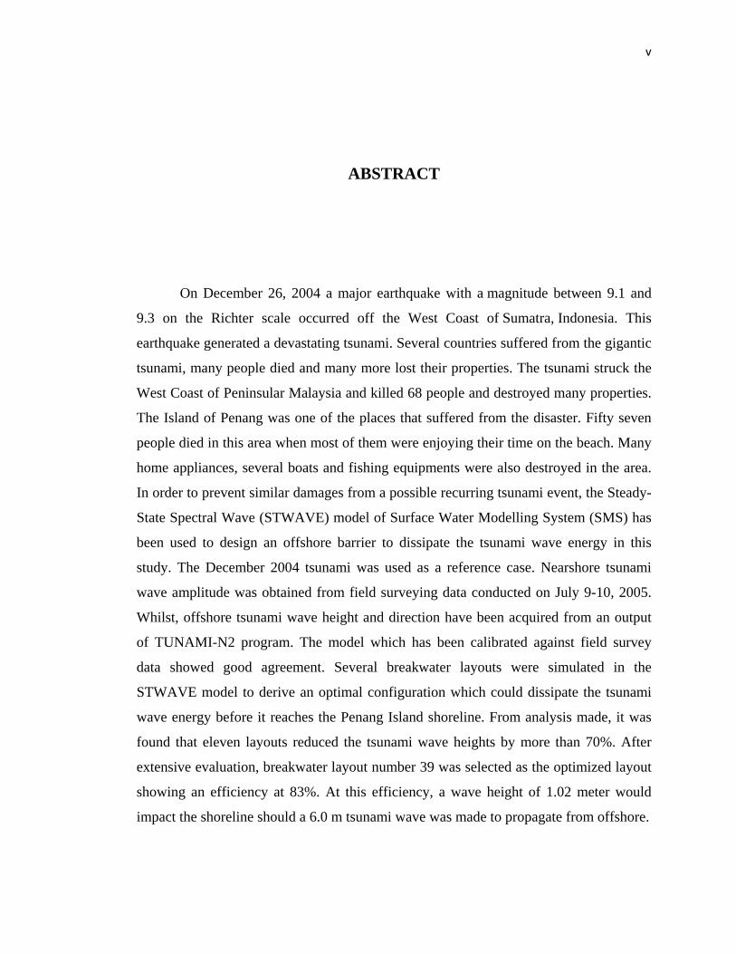
ABSTRACT  

 

 

On December 26, 2004 a major earthquake with a magnitude between 9.1 and

9.3 on the Richter scale occurred off the West Coast of Sumatra, Indonesia. This

earthquake generated a devastating tsunami. Several countries suffered from the gigantic

tsunami, many people died and many more lost their properties. The tsunami struck the

West Coast of Peninsular Malaysia and killed 68 people and destroyed many properties.

The Island of Penang was one of the places that suffered from the disaster. Fifty seven

people died in this area when most of them were enjoying their time on the beach. Many

home appliances, several boats and fishing equipments were also destroyed in the area.

In order to prevent similar damages from a possible recurring tsunami event, the Steady-

State Spectral Wave (STWAVE) model of Surface Water Modelling System (SMS) has

been used to design an offshore barrier to dissipate the tsunami wave energy in this

study. The December 2004 tsunami was used as a reference case. Nearshore tsunami

wave amplitude was obtained from field surveying data conducted on July 9-10, 2005.

Whilst, offshore tsunami wave height and direction have been acquired from an output

of TUNAMI-N2 program. The model which has been calibrated against field survey

data showed good agreement. Several breakwater layouts were simulated in the

STWAVE model to derive an optimal configuration which could dissipate the tsunami

wave energy before it reaches the Penang Island shoreline. From analysis made, it was

found that eleven layouts reduced the tsunami wave heights by more than 70%. After

extensive evaluation, breakwater layout number 39 was selected as the optimized layout

showing an efficiency at 83%. At this efficiency, a wave height of 1.02 meter would

impact the shoreline should a 6.0 m tsunami wave was made to propagate from offshore.

vi  

ABSTRAK  

Pada tanggal 26 Disember 2004, satu gempa bumi dengan magnitud antara

9.1dan 9.3 pada skala Ritcher telah melanda pantai barat Sumatera, Indonesia. Gempa

bumi yang kuat ini telah menyebabkan kejadian tsunami berlaku. Beberapa buah negara

telah terkena tempias tsunami yang mana banyak kematian dan kemusnahan harta benda

telah direkodkan. Malaysia juga tidak terkecuali daripada kejadian tersebut di mana

tsunami telah menyerang pantai barat Semenanjung Malaysia, membunuh sebanyak 68

nyawa dan memusnahkan sebahagian harta benda. Pulau Pinang merupakan di antara

negeri yang paling teruk dilanda gempa bumi ini di Malaysia. Lima puluh tujuh orang

meninggal dunia semasa kebanyakan mereka sedang menghabiskan masa di kawasan

perairan pantai. Bagi menangani kemusnahan yang hampir serupa daripada

kemungkinan kejadian tsunami berulang, model komputer STWAVE (Steady-State

Spectral Wave) yaug terdapat di dalam pakej SMS (Surface Water Modelling System)

telah digunakan untuk merekabentuk struktur airdalam bagi melemahkan tenaga ombak

tsunami di dalam kajian ini. Kejadian tsunami pada Disember 2004 digunakan sebagai

titik rujukan. Gelombang ombak tsunami dekat pantai telah diperolehi daripada data

ukur tapak yang telah dilakukan pada 9-10 Julai 2005. Manakala ketinggian dan arah

ombak diperolehi daripada hasil program TUNAMI-N2. Model yang telah dikalibrasi

dengan data ukur tapak telah menunjukkan persetujuan yang baik. Beberapa konfigurasi

pemecah ombak yang tenggelam telah disimulasi dengan menggunkan model STWAVE

untuk menghasilkan konfigurasi optimal yang dapat melemahkan tenaga ombak tsunami

sebelum menghampiri pantai di Pulau Pinang. Daripada analisis yang dilakukan,

terdapat sebelas pelan pemecah ombak berupaya menghasilkan kecekapan melebihi 70%

untuk melemahkan tenaga ombak tsunami. Pelan kedudukan pemecah ombak yang ke

39 telah dikenalpasti sebagai pelan konfigurasi yang sesuai untuk menyumbang

sebanyak 83% kecekapan. Pada kecekapan ini, jika ombak tsunami setinggi 6 m di

arahkan ke pantai, ketinggian ombak pada 1.02 m akan terhasil di kawasan pantai.

TABLE OF CONTENTS

CHAPTER TITLE PAGE

TITLE PAGE i

DECLARATION ii

DEDICATION iii

ACKNOWLEDGEMENT iv

ABSTRACT v

ABSTRAK vi

TABLE OF CONTENTS vii

LIST OF TABLES x

LIST OF FIGURES xi

LIST OF SYMBOLS xv

LIST OF APPENDICES xvii

I INTRODUCTION

1.1 Tsunami 1

1.2 Tsunami Barriers 2

1.3 Available Computer Models for Wave

Simulation 3

1.4 Problem Statement 4

1.5 Objectives of Study 6

1.6 Scope of Study 7

viii

II LITERATURE REVIEW

2.1 Tsunami 9

2.2 Causes of Tsunami Generation

2.2.1 Earthquakes

11

11

2.2.2 Landslides

2.2.3 Volcanic Eruptions

2.2.4 Meteor Impacts

15

16

17

2.3 Propagation of Tsunami Wave 17

2.4 The Interaction of Tsunami Wave with

Structures

2.4.1 Submerged Breakwater

2.4.2 Wave Transmission over Low-

Crested Structures (LCS)

20

20

24

2.5 The December 2004 Tsunami Event 27

III METHODOLOGY

3.1 Introduction 31

3.2 Design of the Rubblemound Breakwater 33

3.2.1 Breakwater Design Description 35

3.2.2 Design Parameters 35

3.2.3 Breakwater Design Procedure 36

3.3 Surface Water Modeling System (SMS) 40

3.3.1 Steady State Spectral Wave Model

(STWAVE Model)

41

3.3.2 Model Assumption and Limitation 42

3.3.3 Governing Equation of STWAVE 44

3.3.4 Numerical Discretization 46

3.3.5 Model Input and Output Files 47

3.3.5.1 Model Parameter File 48

3.3.5.2 Bathymetry File 48

3.3.5.3 Incident Wave Spectra

File

49

ix

IV DATA COLLECTION AND STWAVE

MODEL SETUP

4.1 Introduction 50

4.2 Data Collection 51

4.2.1 Bathymetric Data 51

4.2.2 Tsunami Wave Data 52

4.3 Generating Input Files 54

4.3.1 Application of Surfer Version 8.0 54

4.3.1 Application of Surface Water

Modeling System (SMS) Version

8.1 56

4.4 STWAVE Model Calibration 62

V DISCUSSION AND ANALYSIS OF THE

COMPUTATIONAL RESULTS

5.1 Introduction 65

5.2 Proposed Breakwater Layout and

Optimization 66

VI CONCLUSIONS AND

RECOMMENDATIONS

6.1 Conclusions 81

6.2 Recommendations 82

LIST OF REFERENCES 83

LIST OF APPENDICES

Appendix A 86

x

LIST OF TABLES

TABLE NO. TITLE PAGE

2.1 Summary of the ranges of parameters involved in 2D wave transmission tests at LCS 26

2.2 Damage and casualties due to the tsunami 2004

event 28

4.1 Results obtained upon calibration of the model 64 5.1 Details of various layouts generated to test for

efficiency as modeled in STWAVE 67 5.2 Performance of proposed breakwater layouts to

attenuate the tsunami wave height 71 5.3 Details of the tsunami wave heights at the

shoreline for barriers which performed at greater than 70% efficiency 74

xi

LIST OF FIGURES

FIGURE NO. TITLE PAGE

1.1 Tsunami disaster in Pulau Pinang 5 1.2 Location of the study area showing the coastline

to the North of Penang Island 7

2.1 Terminology of tsunami waves 10 2.2 Different types of faults which can generate an

earthquake 12 2.3 Tsunami generated by a normal fault 13 2.4 Rough estimates of the tsunami parameters in

the source versus earthquake magnitude using eqn. 2.1 14

2.5 Rough estimates of the tsunami parameters in

the source versus earthquake magnitude using eqn. 2.2 14

2.6 Typical changes in tsunami wave as it reaches

shallow water 18 2.7 Wave reduction caused by a submerged

structure 21 2.8 Wave transmission over reef structure in Amwaj

project 22 2.9 Wave propagation passing over (a) rigid mound

(b) flexible mound 23 2.10 Definitions of governing parameters involved in

wave transmission through LCS 25

xii

2.11 Typical armour type for submerged breakwater used in Van der Meer et al’s research works 26

2.12 Countries affected by the 2004 tsunami 28 2.13 Some of the tsunami affected areas in Penang 30 3.1 Flowchart of the proposed methodology 32 3.2 Parameters used in rubblemound design 36 3.3 Rubblemound section for seaward wave

exposure with zero-to-moderate overtopping conditions 38

3.4 Rubblemound section for wave exposure on

both sides with moderate overtopping conditions 39

3.5 Schematic grid of STWAVE 46 3.6 Schematic input/output files of STWAVE 47 4.1 Bathymetry map of study area 52 4.2 Offshore tsunami wave height generated using

TUNAMI N2 53 4.3 Tsunami wave direction generated using

TUNAMI N2 53 4.4 Application of SURFER to generate an ASCII

XYZ file for the study area 54 4.5 Contour map of study area as generated by

SURFER Version 8.0 55 4.6 3D seabed surface within study area as

generated by SURFER Version 8.0 55 4.7 Wire frame map of study area as generated by

SURFER Version 8.0 56 4.8 Window for opening the ASCII XYZ file in

SMS 57 4.9 Window for registering the bathymetry map of

the study area 58 4.10 Window to set the coverage type to STWAVE 59

xiii

4.11 Creating a polygon around the land 60 4.12 Map to 2-D grid window 60 4.13 Generated 2-D grid for the study area 61 4.14 STWAVE model control windows 62 4.15 Points used in the calibration works 63 4.16 Plot showing observed and computed wave

heights at the location points 64 5.1 Typical outputs of wave heights generated by

STWAVE for the existing condition without any structure 66

5.2 Distribution of wave height on the shoreline due

to the presence of breakwater layout 1 69 5.3 Distribution of wave height along the shoreline

due to the presence of breakwater with two arms 70 5.4 Distribution of wave height on the shoreline due

to the presence of (a) layout 12 (b) layout 26 (c) layout 31 (d) layout 32 (e) layout 34 (f) layout 35 75

5.5 Distribution of wave height on the shoreline due

to the presence of (a) layout 36 (b) layout 37 (c) layout 38 (d) layout 39 76

5.6 Attenuation of tsunami wave height on the

shoreline for without structure and with layouts 11, 12 and 26 conditions 77

5.7 Attenuation of tsunami wave height on the

shoreline for without structure and with layouts 31, 32 and 34 conditions 77

5.8 Attenuation of tsunami wave height on the

shoreline for without structure and with layouts 35, 36 and 37 conditions 78

5.9 Attenuation of tsunami wave height on the

shoreline for without structure and with layouts 38 and 39 conditions 78

5.10 Plan of the optimized breakwater for layout

no.39 79

xiv

5.11 Cross section of segment A for layout no.39 79 5.12 Cross section of segment B for layout no.39 80 5.13 Distribution of tsunami wave on the shoreline

with the construction of breakwater layout no. 39 80

xv

LIST OF SYMBOLS

B - Crest width

Bt - Toe apron width

C - Wave celerity

Dn50 - Nominal diameter of armour rock

d - Water depth

E - Energy density in a given frequency and direction

g - Gravitational acceleration

H - Wave height

He - Water displacement

Hi - Incident significant wave height

H0 - Wave height at deep water

Hr - Wave run-up

Hr max - Maximum tsunami run-up

Hs - Significant wave height in front of breakwater

Ht - Transmitted significant wave height

h - Water elevation

hc - Breakwater crest relative to DHW / structure height

ht - Depth of structure toe relative to still water level

J - Grid row index

K - Wave number

Kt - Transmission coefficient

L - Wave length

L0 - Wave length in deep water

Lc - Wave length on the crest

Lh - Wave length at the toe

xvi

Lom - Deepwater wave length corresponding to mean wave period

Lop - Deepwater wave length corresponding to peak wave period

M,Mw - Earthquake magnitude

Mp,Mu - Overturning moment around the heel

N - Total number of armour layer

Nod - Number of units displaced out of the armour layer

Ns - Number of wave

Ns* - Spectral stability number

P - Notional permeability

P - Wave pressure

Rc - Crest freeboard

Re - Effective radius

S - Arch length, Relative eroded area

Sm, Sop - Wave Steepness

T - Wave period

Tp - Peak period

t - Thickness of layers

tan α - Seaward slop of structure

U - Uplift force

u,v - Velocity

W - Armour unit weight

x,y - Orthogonal horizontal coordinate

α - Front slope (seaside)

αb - Back slope (lee)

δ - Direction of current relative to a reference frame

ζ,η* - Height of free surface above the still water level

ζop - Breaker parameter

η - Wave elevation

ρs - Mass density of rock

ρw - Mass density of water

ω - Angular frequency

xvii

LIST OF APPENDICES

APPENDIX TITLE PAGE

A Details of the tsunami wave heights at the

shoreline for all the proposed layouts 86

1  

CHAPTER 1  

 

 

 

INTRODUCTION

1.1 Tsunami

Tsunami is a Japanese word which means a “harbour wave”. The first

character (Tsu) means harbour and the second character (Nami) means wave. It is a

series of waves created when a body of water is rapidly displaced. In the past

tsunami waves were referred to as tidal waves by the general public and as seismic

sea waves by the scientific community. Although a tsunami wave impact upon a

coastline is dependent upon the tidal level at the time a tsunami strikes, it cannot be

named as tidal wave since tides result from the imbalanced gravitational influences

of the moon, sun and earth system.

2  

Tsunami can be generated by many causes such as earthquakes, submarine

landslides, volcanic activities, under water explosion and asteroid falls. Tsunami

cannot be felt in the open ocean due to its long wave length but as it leaves the deep

water and propagates into shallower water near the coast, it undergoes

transformations, its speed reduces and its wave height increases. Perhaps this natural

disaster cannot be prevented but its result and effects can be reduced through proper

planning.

1.2 Tsunami Barriers  

 

Different types of breakwaters, seawalls and even soft structures may provide

protection against tsunamis. It may decrease the inundation on land as well as reduce

the current velocities and wave magnitude. However, structures may also have

undesired effects on other areas (by reflection) or even on the area to be protected,

because it may affect the resonant period of bays and harbours so that wave height

increases instead of decreases. The energy of a tsunami wave, which is either

dissipated on land or reflected when there is no structure, must now be dissipated by

the structure (Van der Plas 2007).

Different types of structures which can be used for protection against tsunami waves

include:

(a) High-crested structures which have a crest-level that is at least

comparable with the height of the tsunami such as:

Vertical walls

Rubble-mound structures

(b) Low-crested and submerged structures (LCS) such as :

Detached breakwater

Artificial reefs

3  

(c) Soft structures such as:

Mangroves

Sea grasses

1.3 Available Computer Models for Wave Simulation

There are many different types of public domain and commercial software

available which can be used for wave modelling such as SWAN and STWAVE

model as well as CGWAVE model of the Surface-Water Modelling System (SMS).

SWAN is a third-generation wave model which can be used for estimating wave

parameters in coastal areas, lakes and estuaries from given wind, bottom and current

conditions. It also can be used on any scale relevant for wind-generated surface

gravity waves. This model is based on the wave action balance equation with sources

and sinks (Delft University of Technology 2008). CGWAVE is a model developed at

the University of Maine under a contract for the U.S. Army Corps of Engineers,

Waterways Experiment Station. It is a finite-element model that is interfaced to the

SMS model for graphics and efficient implementation. This model can be used for

estimation of wave fields in harbours, open coastal regions, coastal inlets, around

islands and around fixed or floating structures (Demirbilek and Panchang 1998).

STWAVE is a steady-state finite difference model based on the wave action

balance equation and it is formulated on a Cartesian grid. STWAVE simulates

depth-induced wave refraction and shoaling, current induced refraction and shoaling,

depth- and steepness-induced wave breaking, diffraction, wind-wave growth, wave-

wave interaction and whitecapping that redistribute and dissipate energy in a growing

wave field (Smith et al 2001).

4  

As mentioned in the previous paragraphs there are different types of models

which can be used for this research. But owing to availability, only the STWAVE of

SMS will be used for this research work.

1.4 Problem Statement

Tsunamis are infrequent high impact events. They are among the most

terrifying and complex physical phenomena which can cause a considerable number

of fatalities, major damages and significant economic losses.

Horikawa and Shuto (1981) used tsunami damage official records to

categorise the disaster caused directly by the tsunami. They summarized this into the

following groups:

(a) Death and injury.

(b) House destroyed, partly destroyed, inundated or flooded and burned.

(c) Property damage and loss.

(d) Boats washed away, destroyed and run on the rocks.

(e) Lumber washed away.

(f) Marine installations destroyed.

(g) Disastrous damage of public utilities such as roads, electric power supply

installations and water supply installation.

Secondary damages that are indirectly caused by the tsunami can also be

divided into four groups:

5  

(a) Burning houses, oil tank and gas stations

(b) Drifting matter such as houses, lumber, boats, drums, automobiles and sea

culture nursery rafts

(c) Environmental pollution caused by drifting materials, oil, polluted sea bed

and epidemic prevention

(d) Traffic obstruction due to the destruction of roads and railways

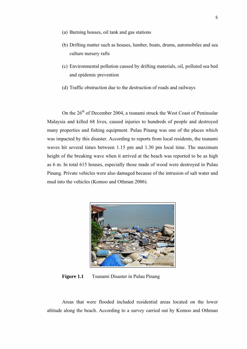
On the 26th of December 2004, a tsunami struck the West Coast of Peninsular

Malaysia and killed 68 lives, caused injuries to hundreds of people and destroyed

many properties and fishing equipment. Pulau Pinang was one of the places which

was impacted by this disaster. According to reports from local residents, the tsunami

waves hit several times between 1.15 pm and 1.30 pm local time. The maximum

height of the breaking wave when it arrived at the beach was reported to be as high

as 6 m. In total 615 houses, especially those made of wood were destroyed in Pulau

Pinang. Private vehicles were also damaged because of the intrusion of salt water and

mud into the vehicles (Komoo and Othman 2006).

Figure 1.1 Tsunami Disaster in Pulau Pinang

Areas that were flooded included residential areas located on the lower

altitude along the beach. According to a survey carried out by Komoo and Othman

6  

(2006) all observed areas showed evidence of flooding, such as mud marks on

buildings walls or mangrove trees, as well as damage to plants due to inundation. In

the coastal area, flood levels reached up to 1.5 m. The flood water which contained

mud damaged many agriculture and ornamental plants along the coastline.

To prevent similar damages due to the recurrence of tsunami wave as

mentioned above to Pulau Pinang, the present research work will focus on

undertaking a computer model investigation to design an offshore structure to

dissipate the tsunami wave energy before it reaches the shoreline. In the present work

the STWAVE module of SMS will be used due to its availability.

1.5 Objectives of Study

The objectives of this project are:

(a) To determine and design an appropriate layout of an offshore barrier to

dissipate the tsunami wave energy along the shoreline to the north of

Penang Island.

(b) To execute a computer model in particular the STWAVE module of

Surface Water Modelling System (SMS) to evaluate the performance of

the optimized structure layout in dissipating the tsunami wave energy.

7  

1.6 Scope of Study

This study is limited to the following scope of work in order to meet the

specified objectives:

(a) To collect existing data and information relevant to the Study Area, that is

the shoreline to the north of Penang Island.

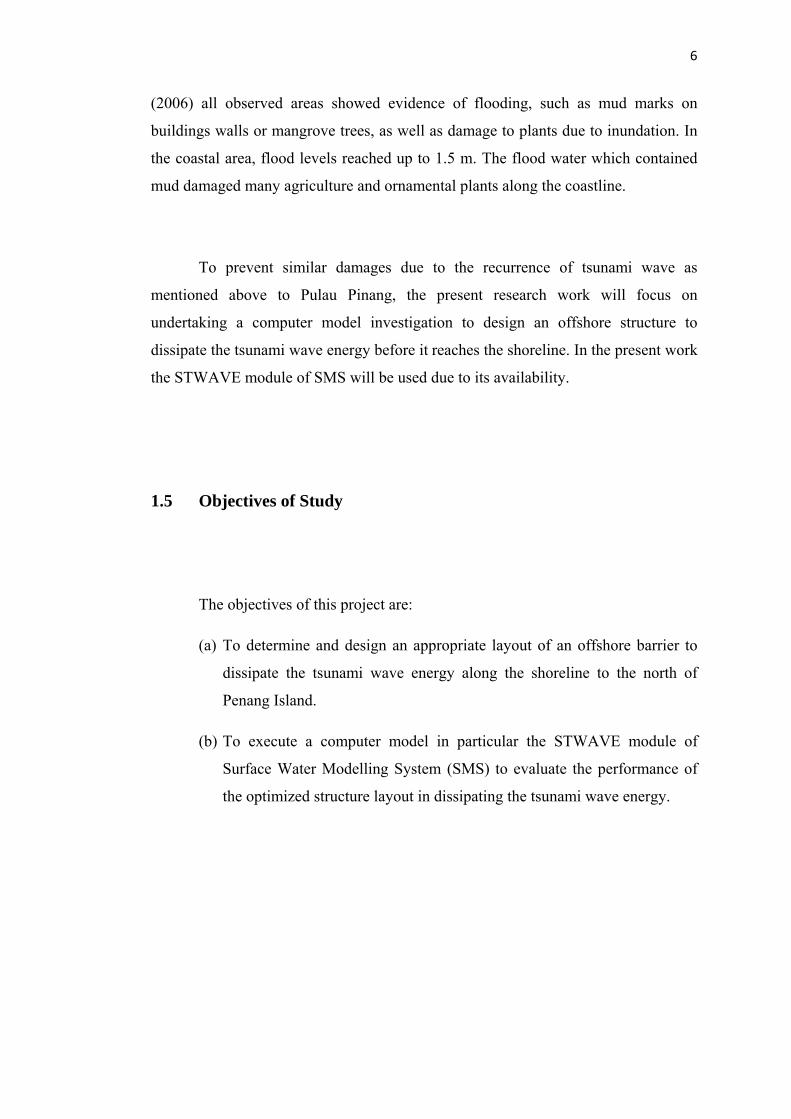
(b) To design offshore barriers to dissipate the tsunami wave energy at three

points namely points 1, 2 and 3 as shown in Figure 1.2.

(c) To evaluate the response of tsunami wave energy around the barrier by

running a computer model typically the STWAVE model of SMS.

Figure 1.2 Location of the Study Area Showing the Coastline to the North of

Penang Island

8  

The three points to be considered in the study area will include:

• Point 1: Point 1 which fronts a wide coastal area which is open and

vulnerable to tsunami waves.

• Point 2: There are two headlands near this point from which waves

can cause damage to the pocket beach.

• Point 3: This coast accommodates a residential area.

 

 

  

 

 

 

 

 

 

 

 

 

 

 

 

 

 

9  

CHAPTER 2 

LITERATURE REVIEW  

2.1 Tsunami 

The term tsunami comes from the Japanese word meaning harbour ("tsu", 津)

and wave ("nami", 波). For the plural form, one can either follow ordinary English

practice and add an” s”, or use an invariable plural as in Japanese. Tsunamis are

common throughout Japanese history; approximately 195 events in Japan have been

recorded. More than 1000 events occurred in the Pacific and about 100 events in the

Atlantic and Indian oceans.

10  

This kind of wave is defined as surface gravity waves. They occur in the

ocean as a result of large-scale short term perturbations. They can be generated by

many causes such as: underwater earthquakes, eruption of underwater volcanoes,

submarine landslides, underwater explosion, rock and asteroid falls, avalanche flows

in the water from land mountains and volcanoes and sometimes drastic changes of

water conditions.

In the open ocean, tsunamis would not be felt by ships because the

wavelength would be hundreds of miles long, with amplitude of only a few feet. This

would also make them unnoticeable from the air. As the waves approach the coast,

their speeds decrease and their amplitudes increase. Unusual wave heights have been

known to be over 30 m high. Waves that are 3 to 6 m high can be very critical and

cause many deaths or injuries. As these waves approach coastal areas, the time

between successive wave crests varies from 5 to 90 minutes. The first wave is

usually not the largest in the series of waves and it is not the most significant one.

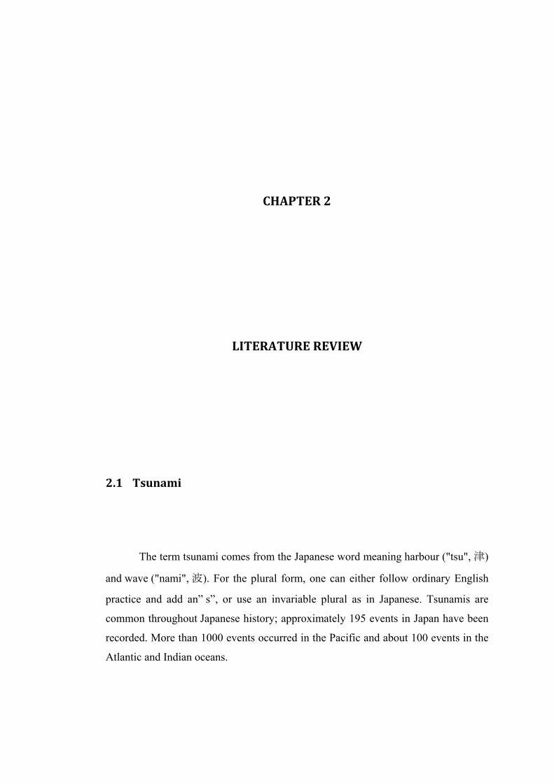
Terminology of the tsunami waves are illustrated in Figure 2.1.

H  =  Wave height (m) Hr  =  Wave run‐up (m) 

h  =  Water elevation (m) η  =  Wave elevation (m) d  =  Water depth (m) H0  =  Wave height in deep water L  =  Wavelength (m) 

Figure 2.1 Terminology of Tsunami Waves (Source: Van der Plas 2007)

11  

2.2 Causes of Tsunami Generation

Tsunami may be generated by different sources. Some of the most important

causes of tsunami generation are as follows:

2.2.1 Earthquakes

Thucydides, a Greek historian was the first person who related tsunami to the

earthquake in 426 BC (Shuto 2001). The most common cause of tsunamis is seismic

activity. Earthquakes are responsible for 75% of all events. Almost all large

earthquakes occur at the boundary of tectonic plates, where one plate slides over

another. Earthquakes can be classified into three types of faults, depending on how

the relative motion of adjacent plates affects the shape of the solid earth. They

include:

(a) Thrust fault- where one tectonic plate moves up and over an adjacent

.....................plate.

(b) Normal fault- occurs when one plate moves down relative to an adjacent

......................plate.

(c) Strike-slip- occurs when they slide past each other horizontally with

................. neither plate being raised or lowered significantly.

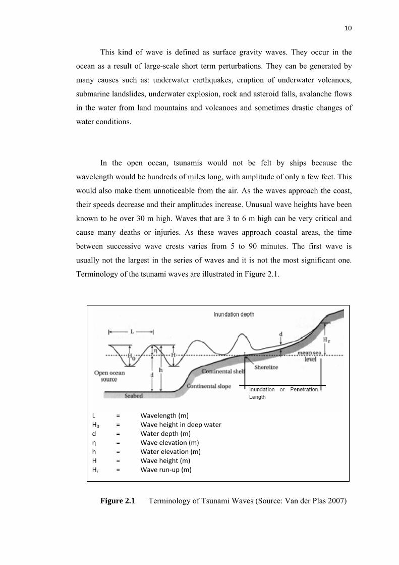
The different types of faults which can generate the tsunami are shown in

Figure 2.2. During tsunami generation, a thrust fault raises the floor of the ocean,

which in turn raises the water above it and creates a positive water wave. A normal

fault lowers the floor of the ocean, so it creates a negative water wave above it.

12  

Strike slip faults do not change the shape of the ocean floor and they do not generate

a tsunami. Therefore the magnitude of an earthquake by itself does not determine

whether that earthquake will generate a significant tsunami (Segur 2006). Figure 2.3

illustrates a fault which causes an earthquake and therefore generates a tsunami.

4

21 

3 

Figure 2.2 Different Types of Faults which can Generate an Earthquake

(Source: Van der Plas 2007)

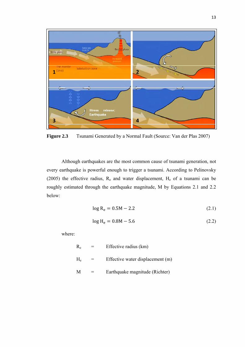
13  

1  2

3  4

Figure 2.3 Tsunami Generated by a Normal Fault (Source: Van der Plas 2007)

Although earthquakes are the most common cause of tsunami generation, not

every earthquake is powerful enough to trigger a tsunami. According to Pelinovsky

(2005) the effective radius, Re and water displacement, He of a tsunami can be

roughly estimated through the earthquake magnitude, M by Equations 2.1 and 2.2

below:

log R 0.5M 2.2

log H 0.8M 5.6 (2.2)

(2.1)

where:

Re = Effective radius (km)

He = Effective water displacement (m)

M = Earthquake magnitude (Richter)

14  

1.00

10.00

100.00

0.00 1.00 2.00 3.00 4.00 5.00 6.00 7.00 8.00 9.00 10.00

Source Rad

ius (Km)

Magnitude (Richter)

Figure 2.4 Rough Estimates of the Tsunami Parameters in the Source Versus

Earthquake Magnitude Using Eqn. 2.1 (Source: Pelinovsky 2005)

0.1

1

10

0.00 1.00 2.00 3.00 4.00 5.00 6.00 7.00 8.00 9.00 10.00

Displacem

en in

 th Sou

rce (m

)

Magnitude (Richter)

Figure 2.5 Rough Estimates of the Tsunami Parameters in the Source Versus

Earthquake Magnitude Using Eqn. 2.2 (Source: Pelinovsky 2005)

From Figures 2.4 and 2.5 it is clear that strong earthquakes with magnitudes

greater than 7 on the Richter scale can generate large tsunami wave several meters in

height and one hundred kilometres in length. For example, an earthquake with a

magnitude of 8.5 Richter can generate a tsunami wave of almost 3.32 meter height

and 7.7 kilometre length at the source.

15  

2.2.2 Landslides

According to Bardet et al (2003), the potential that a major tsunami could be

generated by massive submarine mass failure was recognized a century ago by many

scientists such as Milne (1898) and De Ballore (1907). In recent years, many studies

have supported this idea that a major tsunami could be generated by a large

submarine mass failure itself or triggered by a large earthquake in the coastal area.

Although there is not much information available to describe landslide

tsunami generated events, a few well documented events have helped focus the

attention on landslide generated tsunamis. This includes that during the 1992 Flores

Island, Indonesia earthquake, at the village of Riangkroko, where the run up was

measured to be 26 m, which was the highest on Flores Island. The waves which

destroyed the village and killed 122 people probably originated from a nearby

underwater landslide.

The most usual mechanism of the starting failure of submarine slopes is over

steepening which will happen because of rapid deposition of sediments, generation

of gas created by decomposition of organic matter, storm waves, and earthquakes,

which are the major causes of landslides on continental slopes (Todorovska et al

2001). The failed material is driven by gravity forces.

16  

Not all submarine landslides are capable of generating tsunamis. As

mentioned by Murty (2003) tsunami generation by submarine landslides depends

mainly on the volume of the slide material and to a lesser degree on other factors

such as: angle of the slide, water depth, density and speed of the slide material,

duration of the slide, etc. He also derived a simple linear regression relationship

between H “maximum amplitude of the resulting tsunami” and V “volume of the

slide material” as given in Eqn. 2.3 and 2.4 respectively. Normally, the wavelengths

and periods of landslide-generated tsunami are between 1 to 10 km and 1 to 5

minutes respectively. These values are much shorter than tsunami produced by

earthquakes (Van der Plas 2007).

H 0.3945 V (2.3)

V 2.3994 H (2.4)

where

H = Maximum amplitude of the resulting tsunami (m)

V = Volume of submarine landslide (million m3)

2.2.3 Volcanic Eruptions

Volcanic eruptions can generate tsunami in many different ways. Volcanic

activity can also induce submarine landslides and submarine eruptions/explosions.

Detailed experiments have been performed with underwater explosion with low

energies, when the generated waves have small wave lengths compared with the

water depth (Pelinovsky 2005). For example, the 1952-1953 Mijojin underwater

volcano eruption had energy of 1016 J and caused a tsunami where the parameters of

its source were, Re ≈ 2-3 kilometre and He ≈100-200 meter.

17  

2.2.4 Meteor Impacts

Asteroids larger than 200 meters in diameter hit the earth about every 3000-

5000 years. Most objects smaller than 100 - 200 m in diameter explode in the

atmosphere and will not produce significant waves. Unlike earthquakes the potential

tsunami height caused by meteor-impact is almost unlimited (Van der Plas 2007).

2.3 Propagation of Tsunami Wave

According to Segur (2006), Stokes was the first scientist who developed a

mathematical theory for water waves. He wrote down the equations for the motion of

an incompressible, inviscid fluid, subject to a constant gravitational force, in which

the fluid was bounded below by a rigid bottom and above by a free surface.

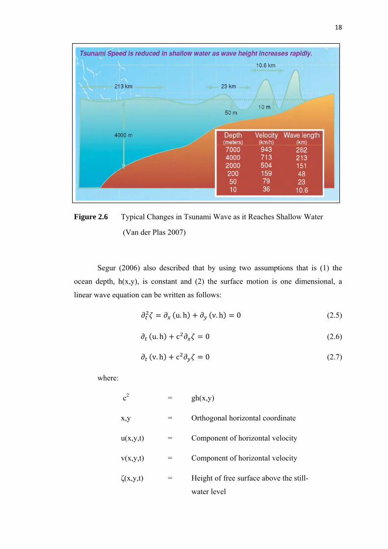
As discussed by Segur (2006) linear wave equation can be used to describe

the propagation of the tsunami far from the shoreline. In the coastal regions as water

depth decreases, wave lengths become shorter and wave amplitude becomes larger as

illustrated in Figure 2.6. Therefore the linear equations are not valid for use any

longer.

18  

Figure 2.6 Typical Changes in Tsunami Wave as it Reaches Shallow Water

(Van der Plas 2007)

Segur (2006) also described that by using two assumptions that is (1) the

ocean depth, h(x,y), is constant and (2) the surface motion is one dimensional, a

linear wave equation n i n s oca be wr tte a foll ws:

v. h 0 (2.5) u. h

(2.6) u. h c 0

v. h c 0 (2.7)

where:

c2 = gh(x,y)

x,y = Orthogonal horizontal coordinate

u(x,y,t) = Component of horizontal velocity

v(x,y,t) = Component of horizontal velocity

ζ(x,y,t) = Height of free surface above the still-

water level

19  

If the surface motion happens to be one dimensional then v in Equations 2.5

and 2.7 will be zero and can be ignored. Therefore, Equations 2.5 to 2.7 can be

combined into a si g ion le equivalent equat n:

. , . , (2.8)

Equation 2.8 is a two dimensional linear wave equation, with a spatially

variable speed of propagation. It can be solved numerically by a variety of methods.

Some conclusions can be drawn directly from the structure of this equation even

without solving it numerically.

One of the important conclusions that could be derived is that any solution of

Equation 2.8 propagate with local speed

c g. h x, y (2.9)

where:

c = Wave celerity (m/s)

g = Gravitational acceleration (m/s²)

h(x,y) = Water displacement (m)

Also the time required for a wave that starts at the epicentre of the earthquake

to reach any particular coastal region can be determined by

T,

(2.10)

where:

s = Arch length along the given starting point to the

identified coastal region

20  

c = Wave celerity (m/s)

T = Wave propagation time (s)

2.4 The Interaction of Tsunami Wave with Structures

As presented in Section 1.2, there are different types of structures which can

be used to protect coastal areas against tsunami waves. The energy of a tsunami

wave, which is either dissipated on land or reflected when there is no structure, must

now be reflected by the structure. The resulting forces on the structure as well as

current velocities depend highly on the wave height and waveform. The effect of

waves and wave transition over some types of structures is described in the following

sections.

 

2.4.1 Submerged Breakwaters

The efficiency of submerged structures and the resulting shoreline response

mainly depends on transmission characteristics and the layout of the structure.

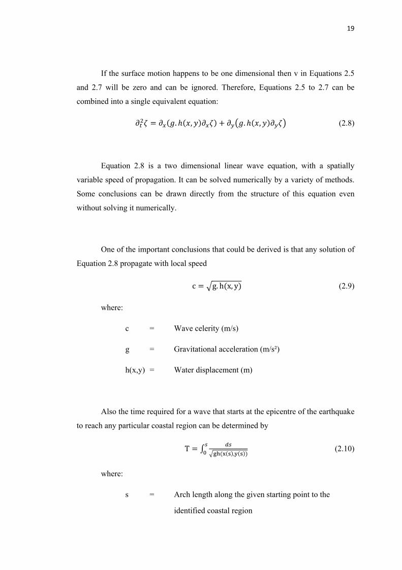
Pilarczyk (2003) gives an overview of the formula to determine the wave

transmission coefficient KT for different values of relative crest width, B/L0, and

crest height, Rc/Hsi, where Rc is the height of the breakwater above water level and

Hsi is the incident significant wave height (refer to Figure 2.7)

21  

Figure 2.7 Wave Reduction Caused by a Submerged Structure (Source: Pilarczyk 2003)

The wavelength on the crest can be determined by Lc= 0.5Tp(gRc), at the toe

by Lh= 0.5Tp(gRc) and in deepwater by Lo=gT2/2π .In order to find the efficiency of a

submerged breakwater he used the Lc definition (instead of Lo) and two numerical

coefficients that is, C=0.64 for a permeable and C=0.80 for an impermeable structure

in the original d’Angremond et al (1996) formula as given by Equation 2.11. By

using this equation he found a good agreement between calculated wave transmission

and the measured one for The Amwaj Islands Development Project in Bahrain. The

Amwaj Islands Development Project involves the construction of new islands on the

existing coral reef. In order to protect the waterfront developments on the mentioned

island from wave attack a submerged breakwater was proposed. The wave

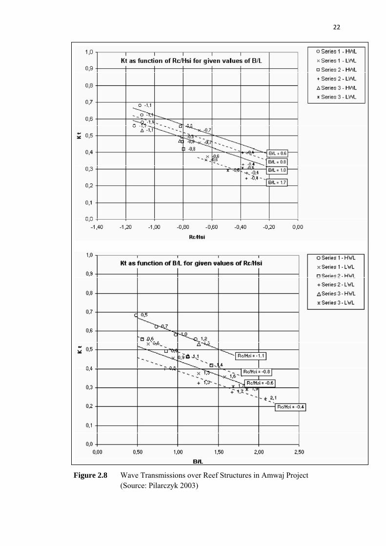
transmission for the proposed submerged breakwater is illustrated in Figure 2.8 and

demonstrated that the effectiveness of a submerged structure depended on the ratio

B/L and Rc/Hsi. Decreasing these ratios would increase the transmission and thus

decrease the effectiveness of the structure. The wave transmission over a submerged

breakwater formula is given by:

K 0.4 RH

0.64 BH

.1 e . (2.11)

where

Kt = Transmission coefficient

Rc = Crest freeboard (m)

Hsi = Incident significant wave height (m)

B = Crest width (m)

ζ = Surf similarity parameter

22  

Figure 2.8 Wave Transmissions over Reef Structures in Amwaj Project

(Source: Pilarczyk 2003)

23  

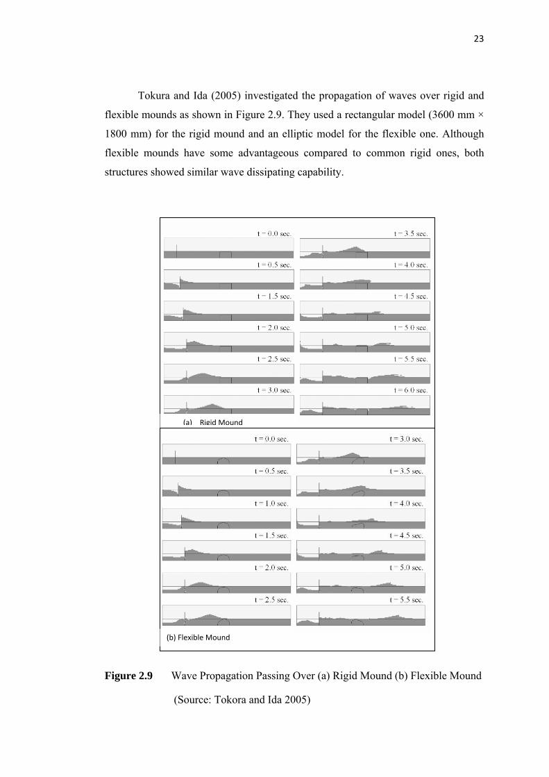
Tokura and Ida (2005) investigated the propagation of waves over rigid and

flexible mounds as shown in Figure 2.9. They used a rectangular model (3600 mm ×

1800 mm) for the rigid mound and an elliptic model for the flexible one. Although

flexible mounds have some advantageous compared to common rigid ones, both

structures showed similar wave dissipating capability.

(a) Rigid Mound

(b) Flexible Mound 

Figure 2.9 Wave Propagation Passing Over (a) Rigid Mound (b) Flexible Mound

(Source: Tokora and Ida 2005)

24  

2.4.2 Wave Transmission Over Low-Crested Structures (LCS)

Waves propagating from deep water may reach a structure after refraction,

shoaling and breaking. As soon as the waves reach a structure, they undergo several

processes. The waves may break on the structure, overtop it, generate waves behind

the structure and reflect from the structure. Also waves may penetrate through

openings between structures. Wave penetration and diffraction do not depend on the

fact whether the structure is low-crested or not. The main effect of an LCS is that

energy can pass over the crest and generate milder waves behind the structure.

There are at least 14 variables which control the relationship between an

offshore breakwater and response of the shoreline. Among these variables eight are

considered primary namely:

(a) distance offshore

(b) length of the structure

(c) transmission characteristics of the structure

(d) beach slope and/or depth at the structure (controlled in part by the sand

grain size)

(e) mean wave height

(f) mean wave period

(g) orientation angle of the structure

(h) predominant wave direction

For segmented detached breakwaters and artificial reefs, the gap between

segments becomes another primary variable. The main parameters that can describe

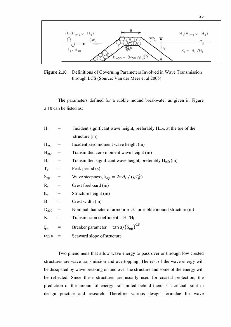
wave transmission over a low crested breakwater are illustrated in Figure 2.10.

25  

Figure 2.10 Definitions of Governing Parameters Involved in Wave Transmission

through LCS (Source: Van der Meer et al 2005)

The parameters defined for a rubble mound breakwater as given in Figure

2.10 can be listed as:

Hi = Incident significant wave height, preferably Hm0i, at the toe of the

structure (m)

Hmoi = Incident zero moment wave height (m)

Hmot = Transmitted zero moment wave height (m)

Ht = Transmitted significant wave height, preferably Hm0t (m)

Tp = Peak period (s)

Sop = Wave steepness, 2 /

Rc = Crest freeboard (m)

hc = Structure height (m)

B = Crest width (m)

Dn50 = Nominal diameter of armour rock for rubble mound structure (m)

Kt = Transmission coeff i Hic ent = Ht / i

ζop = Breaker parameter tan a/ S .

tan α = Seaward slope of structure

Two phenomena that allow wave energy to pass over or through low crested

structures are wave transmission and overtopping. The rest of the wave energy will

be dissipated by wave breaking on and over the structure and some of the energy will

be reflected. Since these structures are usually used for coastal protection, the

prediction of the amount of energy transmitted behind them is a crucial point in

design practice and research. Therefore various design formulae for wave

26  

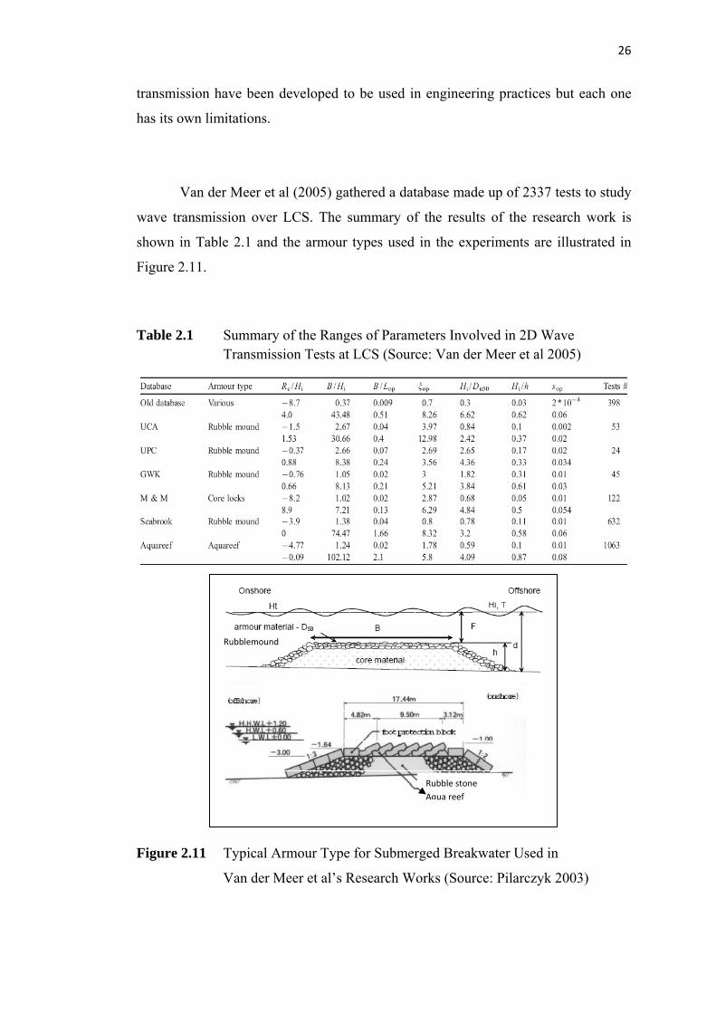
transmission have been developed to be used in engineering practices but each one

has its own limitations.

Van der Meer et al (2005) gathered a database made up of 2337 tests to study

wave transmission over LCS. The summary of the results of the research work is

shown in Table 2.1 and the armour types used in the experiments are illustrated in

Figure 2.11.

Table 2.1 Summary of the Ranges of Parameters Involved in 2D Wave Transmission Tests at LCS (Source: Van der Meer et al 2005)

Rubble stone Aqua reef

Rubblemound 

Figure 2.11 Typical Armour Type for Submerged Breakwater Used in

Van der Meer et al’s Research Works (Source: Pilarczyk 2003)

27  

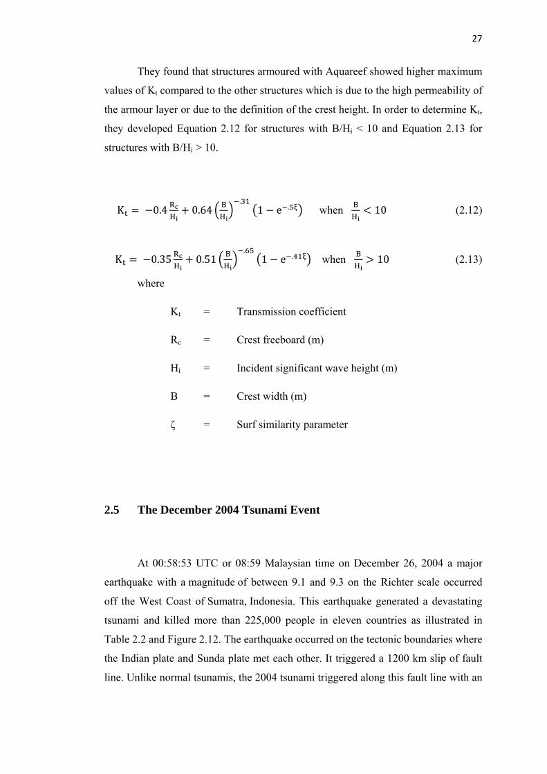
They found that structures armoured with Aquareef showed higher maximum

values of Kt compared to the other structures which is due to the high permeability of

the armour layer or due to the definition of the crest height. In order to determine Kt,

they developed Equation 2.12 for structures with B/Hi < 10 and Equation 2.13 for

structures with B/Hi > 10.

K 0.4 RH

0.64 BH

.1 e . when B

H10 (2.12)

K 0.35 RH

0.51 BH

.1 e . when B

H10 (2.13)

where

Kt = Transmission coefficient

Rc = Crest freeboard (m)

Hi = Incident significant wave height (m)

B = Crest width (m)

ζ = Surf similarity parameter

2.5 The December 2004 Tsunami Event

At 00:58:53 UTC or 08:59 Malaysian time on December 26, 2004 a major

earthquake with a magnitude of between 9.1 and 9.3 on the Richter scale occurred

off the West Coast of Sumatra, Indonesia. This earthquake generated a devastating

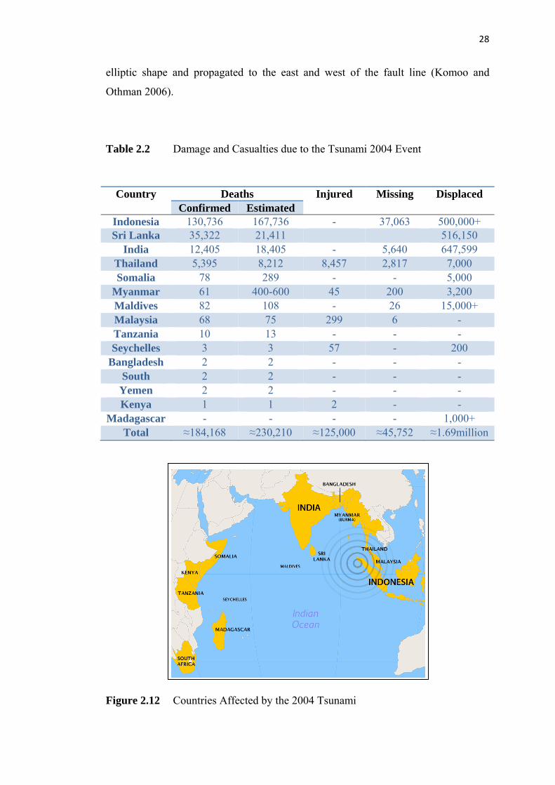
tsunami and killed more than 225,000 people in eleven countries as illustrated in

Table 2.2 and Figure 2.12. The earthquake occurred on the tectonic boundaries where

the Indian plate and Sunda plate met each other. It triggered a 1200 km slip of fault

line. Unlike normal tsunamis, the 2004 tsunami triggered along this fault line with an

28  

elliptic shape and propagated to the east and west of the fault line (Komoo and

Othman 2006).

Table 2.2 Damage and Casualties due to the Tsunami 2004 Event

 

Country Deaths Injured Missing Displaced Confirmed Estimated

Indonesia 130,736 167,736 - 37,063 500,000+ Sri Lanka 35,322 21,411 516,150

India 12,405 18,405 - 5,640 647,599 Thailand 5,395 8,212 8,457 2,817 7,000 Somalia 78 289 - - 5,000

Myanmar 61 400-600 45 200 3,200 Maldives 82 108 - 26 15,000+ Malaysia 68 75 299 6 - Tanzania 10 13 - - - Seychelles 3 3 57 - 200

Bangladesh 2 2 - - - South 2 2 - - -

Yemen 2 2 - - - Kenya 1 1 2 - -

Madagascar - - - - 1,000+ Total ≈184,168 ≈230,210 ≈125,000 ≈45,752 ≈1.69million

Figure 2.12 Countries Affected by the 2004 Tsunami

29  

An earthquake with a magnitude greater than 9.0 had not occurred in this area

since 200 years ago (Van der Plas 2007). It was the second largest earthquake ever

recorded on a seismograph and it had the longest fault duration, between 8.3 and 10

minutes. It caused the entire planet to vibrate as much as 1 cm and triggered other

earthquakes as far away as Alaska. After its generation, it took only a few minutes to

reach the northern shore of North Sumatra while it reached the coastline of Sri Lanka

and the eastern coast of India between 90 to 120 min. The north-western shoreline of

Peninsular Malaysia experienced this disaster after 3 to 4 hours. Due to the

morphology of the Malacca Straits and the reduction of sea water to about 50 meter

the tsunami became more widely disturbed and undergo refraction and reflection.

Therefore its speed and energy decreased and its wave height reduced to 2 to 5 m

(Komoo and Othman 2006).

Pulau Pinang was one of the places in Malaysia which was impacted by this

tsunami. It was believed that the tsunami hit the shoreline of Pulau Pinang several

times between 1.15 p.m. and 1.30 pm on that day. In total, thirteen places in the

western and northern parts of the island had recorded death and loss of property. The

tsunami killed 52 people in Penang. Most of them were trapped while swimming and

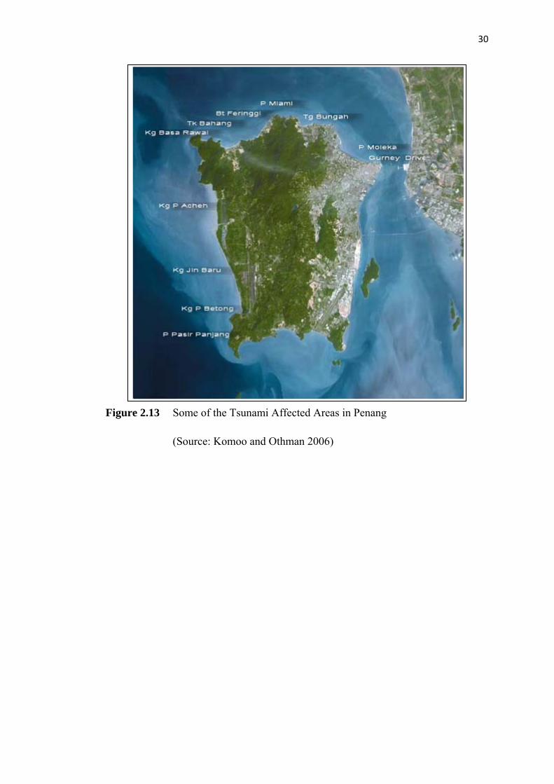
having a picnic on the beach. The areas in Penang affected by the tsunami (see

Figure 2.13) were Kg. Perlis, Kuala Jalan Baru, Kuala Sg. Pinang, Kg. Pantia

Malindo, Kg. Permatang Damar Laut, Kg. Pulau Bentong, Kg. Aceh, Sg. Batu, Kg.

Teluk Kumbar and Pantai Pasir Panjang which are in Balik Pulau to the west of the

Island and the northern coast of Island, i.e. Tg. Bungah, Tg. Tokong, Batu Ferringi,

Teluk Bahang and Pantai Miami (Komoo and Othman 2006). Although many areas

were affected in Penang, the study area sited in this research work is limited to the

Tg. Bungah area only.

30  

Figure 2.13 Some of the Tsunami Affected Areas in Penang

(Source: Komoo and Othman 2006)

31  

CHAPTER 3

METHODOLOGY

3.1 Introduction

The objectives of this research are two fold. The first is to design the layout

of an offshore barrier to dissipate tsunami wave energy. The second objective is to

execute a computer model to evaluate the performance of the structure in dissipating

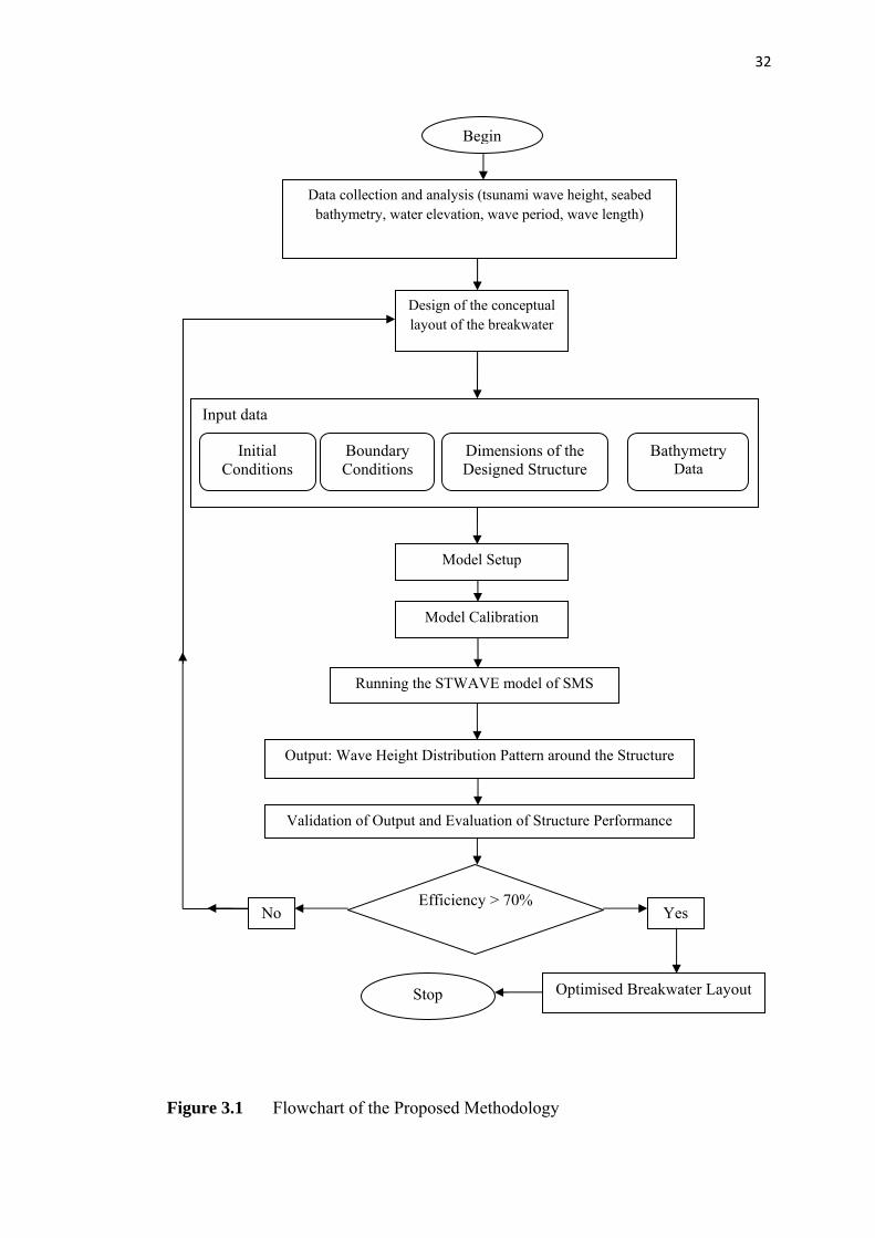
tsunami wave energy at the northern shoreline of Penang Island. The flowchart

shown in Figure 3.1 illustrates the proposed methodology adopted for the present

work. The design criteria utilized and the Surface Water Modelling System which

has been used to simulate wave propagation and to design the wave barrier is

discussed in detail in the following sections.

32  

Begin

Input data

Design of the conceptual layout of the breakwater

Initial Conditions

Boundary Conditions

Dimensions of the Designed Structure

Bathymetry Data

Model Setup

Running the STWAVE model of SMS

Output: Wave Height Distribution Pattern around the Structure

Validation of Output and Evaluation of Structure Performance

Efficiency > 70% Yes

Stop Optimised Breakwater Layout

No

Model Calibration

Data collection and analysis (tsunami wave height, seabed bathymetry, water elevation, wave period, wave length)

Figure 3.1 Flowchart of the Proposed Methodology

33  

Both partially and fully submerged breakwaters can be built as rubblemound

structures (Pencev 2004). In the following sections the design of a rubblemound

structure is discussed in detail.

3.2 Design of the Rubblemound Breakwater

Rubblemound breakwaters can be divided into two main groups. They are

include:

(a) Attached breakwater

(b) Detached breakwater

Due to the location of the shoreline and the area to be protected, the

breakwater can be designed to be attached or detached from the shoreline. An

attached breakwater is a breakwater which is extended from a natural headland and it

could be used to protect a pocket beach. On the other hand detached breakwaters are

those which are small, relatively short, non shore-connected and located near shore

(USACE 2006). If a breakwater were required to protect a coastal area which was

open to offshore waves and major wave crests approached parallel to the coastline, a

detached offshore breakwater might be the better option for use in design (Sheppard

2004).

Both attached and detached breakwaters have their own advantages and

limitations. An advantage of attached breakwaters is that they are easily accessible

for construction, operation and maintenance. However high construction cost and

negative impact on the neighbouring area are two main disadvantages. Detached

34  

breakwaters are more environmental friendly but their construction and maintenance

costs are higher.

According to Sheppard (2004) rubblemound breakwaters can be designed as

overtopped or non-overtopped structures. In overtopped structures, crown elevation

allows larger waves to move across the crest. Overtopped structures are more

difficult to design because their stability response is strongly affected by small

changes in the still water level. In non-overtopped structures the elevation of the

crown prevents any significant amount of wave energy from crossing the crest. They

can provide protection from many waves, but they are more costly to build because

of the increased volume of materials required.

Submerged breakwaters are commonly used for coastal protection and

erosion control at beaches. A desirable feature of submerged breakwaters (and low-

crested structures, in general) is that they do not interrupt the clear view of the sea

from the beach. This aesthetic feature is important for maintaining the touristic value

of many beaches and it is usually one of the considerations in using such structures

for shoreline protection (Prions et al 2004). The main idea of using this type of

structure is to reduce the wave energy reaching the beach by triggering wave energy

dissipation over the structure. In other words, their purpose is to reduce the hydraulic

loading to a required level that maintains the dynamic equilibrium of the shoreline.

To attain this goal, they are designed to allow the transmission of a certain amount of

wave energy over the structure by overtopping and also some transmission through

the porous structure as in permeable breakwaters or wave breaking and energy

dissipation on the shallow crest as at submerged structures (Pilarczyk 2003).

Usually, offshore breakwaters, and especially, the low-crested submerged

structures, provide environmentally friendly coastal solutions. However, high

construction cost and the difficulty of predicting the response of the beach are the

two main disadvantages that inhibit the use of offshore breakwaters.

35  

3.2.1 Breakwater Design Description

A typical breakwater can be described and constructed with at least three

major layers as follows:

(a) Outer layer called the armour layer (this is composed of the largest units,

stone or specially shaped concrete armour units)

(b) One or more stone underlayers.

(c) Core or base layer of quarry-run stone, sand or slag (as bedding or filter

layer below)

The armour layer may need to be covered with specially shaped concrete

armour units (such as Dolos, Tetrapod, Quadripod and Tribar) in order to provide an

economic construction of a stable breakwater (Sheppard 2004).

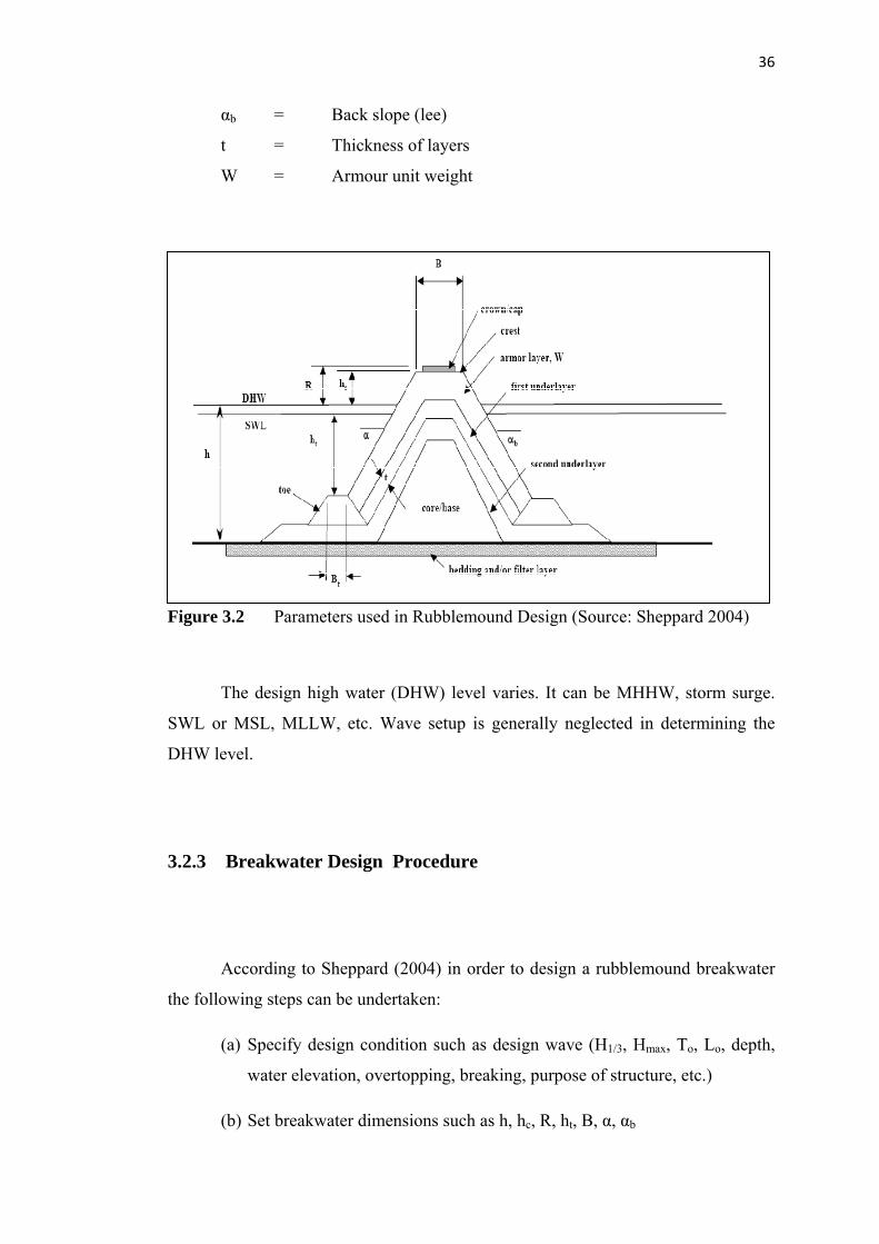
3.2.2 Design Parameters

In order to design a typical rubblemound breakwater there are some

parameters which should be considered and these are shown in Figure 3.2. They

include:

h = Water depth of structure relative to design high water (DHW)

hc = Breakwater crest relative to DHW

R = Freeboard, peak crown elevation above DHW

ht = Depth of structure toe relative to still water level (SWL)

B = Crest width

Bt = Toe apron width

Α = Front slope (seaside)

36  

αb = Back slope (lee)

t = Thickness of layers

W = Armour unit weight

Figure 3.2 Parameters used in Rubblemound Design (Source: Sheppard 2004)

The design high water (DHW) level varies. It can be MHHW, storm surge.

SWL or MSL, MLLW, etc. Wave setup is generally neglected in determining the

DHW level.

3.2.3 Breakwater Design Procedure

According to Sheppard (2004) in order to design a rubblemound breakwater

the following steps can be undertaken:

(a) Specify design condition such as design wave (H1/3, Hmax, To, Lo, depth,

water elevation, overtopping, breaking, purpose of structure, etc.)

(b) Set breakwater dimensions such as h, hc, R, ht, B, α, αb

37  

(c) Determine the armour unit size/ type and under layer requirements.

(d) Develop the toe structure and filter or bedding layer.

(e) Analyze the foundation settlement, bearing capacity and stability.

(f) Adjust parameters and repeat as necessary.

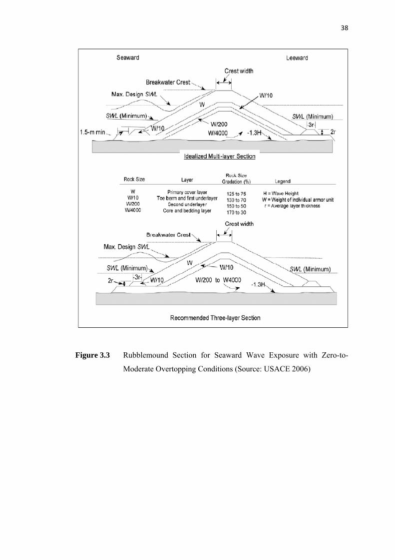
Typical rubblemound cross sections are shown in Figures 3.3 and 3.4 in

which the first figure illustrates the cross-sectional features typical of designs for

breakwaters exposed to waves on one side (seaward) and intended to allow minimal

wave transmission to the leeward side. Breakwaters of this type are usually designed

with crests elevated to allow overtopping only in very severe storms with long return

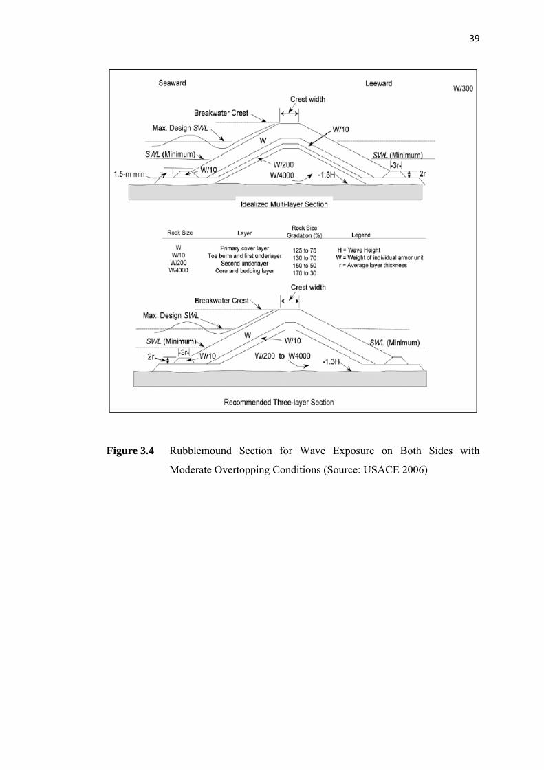
periods. Figure 3.4 shows features common to designs where the breakwater may be

exposed to substantial wave action from both sides and where overtopping is allowed

to be more frequent.

38  

Figure 3.3 Rubblemound Section for Seaward Wave Exposure with Zero-to-

Moderate Overtopping Conditions (Source: USACE 2006)

39  

Figure 3.4 Rubblemound Section for Wave Exposure on Both Sides with

Moderate Overtopping Conditions (Source: USACE 2006)

40  

3.3 Surface Water Modelling System (SMS)

Surface Water Modelling System (SMS) is a graphical program that allows

engineers and scientists to visualize, manipulate and understand numerical data. SMS

comprises one, two, and three dimensional numerical models including finite

element and finite difference models. This software is a product of the environmental

modelling research laboratory of Brigham Young University and new enhancements

and developments continue in cooperation with the U.S. Army Corps of Engineers

(USACE), Engineer Research and Development Centre (ERDC) and the U.S. Federal

Highway Administration (FHWA) (SMS Manual 2004).

 

SMS contains different tools for surface water modelling, analysis and

design. It includes tools for:

(a) Managing, editing and visualizing geometric and hydraulic data

(b) Creating, editing and formatting mesh/grid data for use in numerical

analysis which includes:

(i) Finite Element Meshes (unstructured grids). The tools support:

Linear and quadratic elements.

All triangular or mixture of triangular and quadrilateral

meshes.

Incorporation of 1D elements into 2D and 3D meshes.

(ii) Finite Difference Grids (structured grids). The tools support:

Rectilinear grids at specified rotation.

Boundary fitted (curvilinear) grids.

(iii) Triangulated Irregular Networks (TINS)

Interfaces have been specifically designed to facilitate the utilization of

several numerical models in SMS. Supported models in SMS include:

(a) United States Army Corps of Engineers (USACE)

(i) Engineer Research and Development Centre (ERDC)

TABS-MD (GFGEN, RMA2, RMA4, RMA10, SED2D-

WES)

41  

ADCIRC

CGWAVE

STWAVE (is a steady-state finite difference model based

on the wave action balance equation)

HIVEL2D

CH3D

(ii) Hydrologic Engineering Centre (HEC)

HEC-RAS

(b) Federal Highway Administration (FHWA)

(i) FESWMS-FlO2DH

(c) Independent/Commercial Licenses

(i) M2D

(ii) Generic 2D Finite Element Interface

(iii) Generic 2D Finite Difference Interface

In the SMS manual these models have been described to be able to compute a

variety of information applicable to surface water modelling. The principle

application is hydrodynamic modelling. This involves the calculation of water

surface elevations and flow velocities for shallow water flow problems. It supports

both a steady-state and dynamic model. Additional applications include the

modelling of contaminant migration, salinity intrusion, sediment transport (scour and

deposition), wave energy dispersion, wave properties (directions, magnitudes and

amplitudes) and many others.

3.3.1 Steady-State Spectral Wave Model (STWAVE Model)

Important work components in most coastal projects are to predict

bathymetric and shoreline change, to design or repair coastal structures, to assess

navigation conditions and to estimate the nearshore wave growth and transformation.

Nearshore wave propagation is influenced by many parameters such as complex

42  

bathymetry, tide, wind and wave generated currents, tide and surge induced water

level variation and coastal structures.

The purpose of applying nearshore wave transformation models is to describe

the change in wave parameters for example wave height, period, direction and

spectral shape between the offshore and the nearshore. In relatively deep water, the

wave field is fairly homogeneous on a scale of kilometres; but in the nearshore,

where waves are strongly influenced by variations in bathymetry, water level and

current, wave parameters may vary significantly on the scale of tens of meters.

Offshore wave information is typically available from a wave gauge, or a global

scale or regional scale wave hindcast or forecast (Smith et al 2001).

STWAVE simulates depth-induced wave refraction and shoaling, current

induced refraction and shoaling, depth- and steepness-induced wave breaking,

diffraction, wind-wave growth, and wave-wave interaction and whitecapping that

redistribute and dissipate energy in a growing wave field (Smith et al 2001).

3.3.2 Model Assumptions and Limitations

Like other computer models, STWAVE has been developed based on a few

assumptions. The assumptions made in STWAVE by Smith et al (2001) are as

follows:

(a) Mild bottom slope and negligible wave reflection.

Wave energy in the STWAVE model can only propagate from

offshore towards the nearshore. Therefore waves which are reflected from the

shoreline or from steep bottom features and travel in directions outside this

half plane (from shoreline to the sea) are neglected. Moreover forward-

43  

scattered waves, for example waves reflected off a structure but travelling in

the +x-direction are also neglected.

(b) Spatially homogeneous offshore wave conditions.

The input spectrum in STWAVE is constant along the offshore

boundary because the variation in the wave spectrum along the offshore

boundary with a large domain is expected to be small.

(c) Steady-state waves, currents and winds.

In order to reduce the computation time, STWAVE is formulated as a

steady-state model.

(d) Linear refraction and shoaling.

Only linear wave refraction and shoaling are included is STWAVE,

thus the accuracy of the model is reduced.

(e) Depth-uniform current.

The wave-current interaction is based on a current that is constant

through the water column.

(f) Bottom friction is neglected.

Bottom friction is neglected in STWAVE because determining the

proper friction coefficient is difficult and the cumulative bottom friction

dissipation in nearshore is small.

(g) Linear radiation stress.

Radiation stress in STWAVE is calculated based on linear wave theory.

44  

3.3.3 Governing Equations of STWAVE

Some of the governing equations which are used in STWAVE can be listed as

follows:

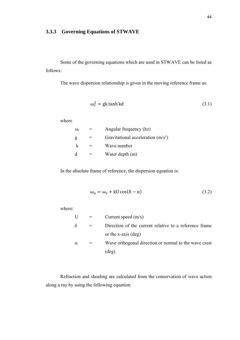
The wave dispersion relationship is given in the moving reference frame as:

ω gk tanh kd (3.1)

where

ωr = Angular frequency (hz)

g = Gravitational acceleration (m/s²)

k = Wave number

d = Water depth (m)

In the absolute frame of reference, the dispersion equation is:

ω ω kU cos δ α (3.2)

where:

U = Current speed (m/s)

δ = Direction of the current relative to a reference frame

or the x-axis (deg)

α = Wave orthogonal direction or normal to the wave crest

(deg)

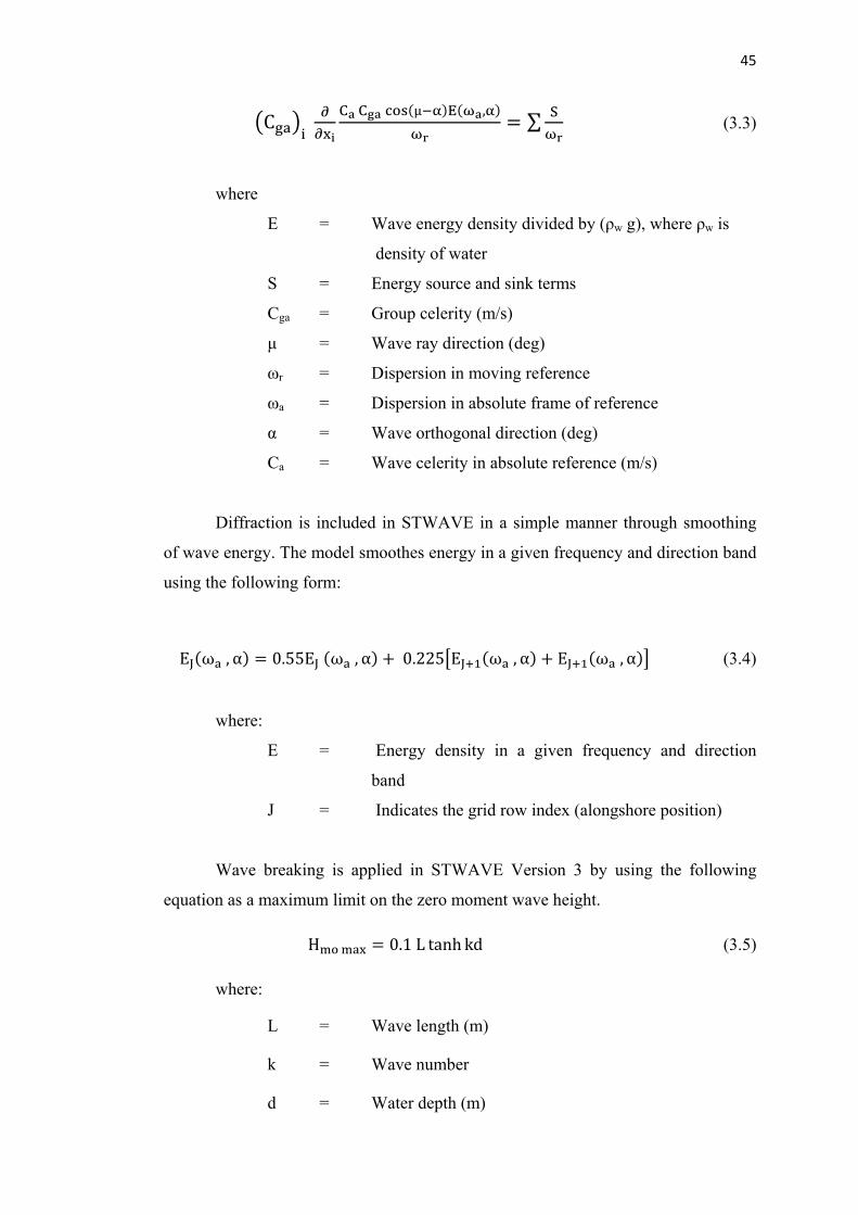
Refraction and shoaling are calculated from the conservation of wave action

along a ray by using the following equation:

45  

C C C µ E , ∑ S (3.3)

where

E = Wave energy density divided by (ρw g), where ρw is

density of water

S = Energy source and sink terms

Cga = Group celerity (m/s)

μ = Wave ray direction (deg)

ωr = Dispersion in moving reference

ωa = Dispersion in absolute frame of reference

α = Wave orthogonal direction (deg)

Ca = Wave celerity in absolute reference (m/s)

Diffraction is included in STWAVE in a simple manner through smoothing

of wave energy. The model smoothes energy in a given frequency and direction band

using the following form:

EJ ω , α 0.55EJ ω , α 0.225 EJ ω , α EJ ω , α (3.4)

where:

E = Energy density in a given frequency and direction

............band

J = Indicates the grid row index (alongshore position)

Wave breaking is applied in STWAVE Version 3 by using the following

equation as a maxim limit nt wave height. um on the zero mome

H 0.1 L tanh kd (3.5)

where:

L = Wave length (m)

k = Wave number

d = Water depth (m)

46  

3.3.4 Numerical Discretization

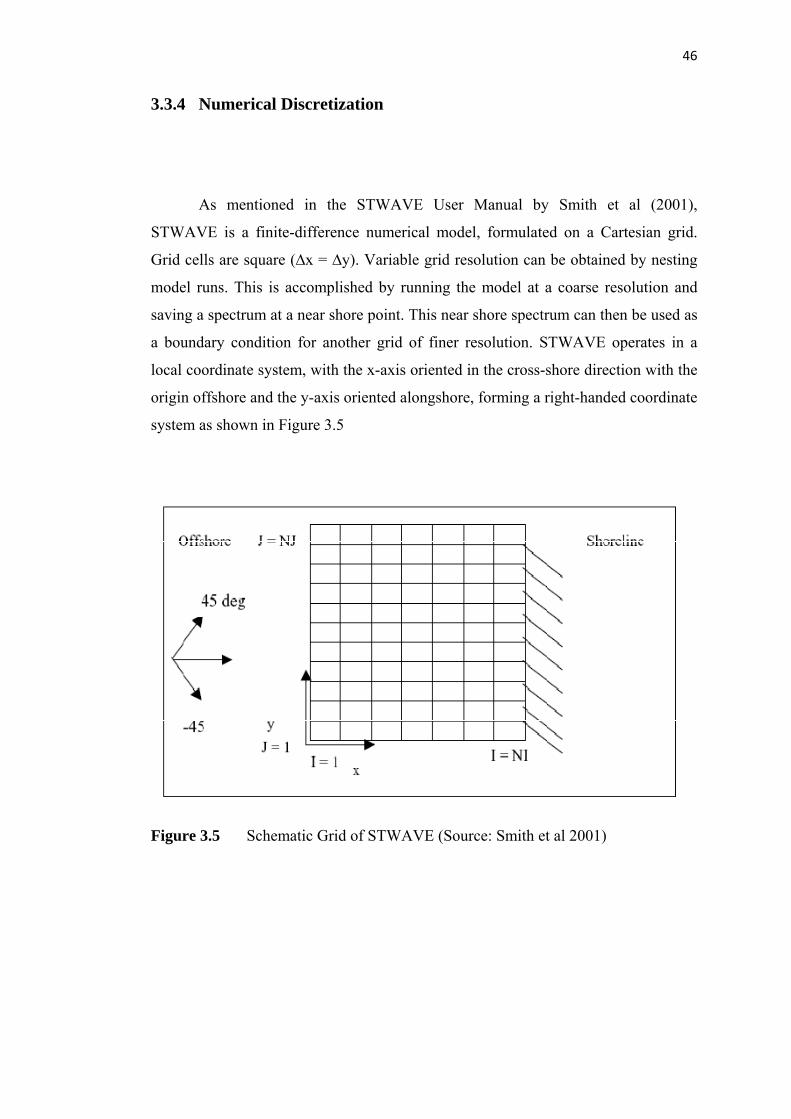
As mentioned in the STWAVE User Manual by Smith et al (2001),

STWAVE is a finite-difference numerical model, formulated on a Cartesian grid.

Grid cells are square (∆x = ∆y). Variable grid resolution can be obtained by nesting

model runs. This is accomplished by running the model at a coarse resolution and

saving a spectrum at a near shore point. This near shore spectrum can then be used as

a boundary condition for another grid of finer resolution. STWAVE operates in a

local coordinate system, with the x-axis oriented in the cross-shore direction with the

origin offshore and the y-axis oriented alongshore, forming a right-handed coordinate

system as shown in Figure 3.5

Figure 3.5 Schematic Grid of STWAVE (Source: Smith et al 2001)

47  

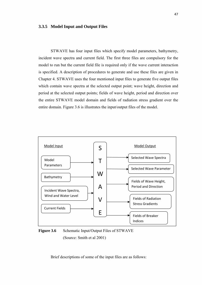
3.3.5 Model Input and Output Files

STWAVE has four input files which specify model parameters, bathymetry,

incident wave spectra and current field. The first three files are compulsory for the

model to run but the current field file is required only if the wave current interaction

is specified. A description of procedures to generate and use these files are given in

Chapter 4. STWAVE uses the four mentioned input files to generate five output files

which contain wave spectra at the selected output point; wave height, direction and

period at the selected output points; fields of wave height, period and direction over

the entire STWAVE model domain and fields of radiation stress gradient over the

entire domain. Figure 3.6 is illustrates the input/output files of the model.

Model Input  Model Output

 

 

 

 

 

 

Figure 3.6 Schematic Input/Output Files of STWAVE

(Source: Smith et al 2001)

 

Brief descriptions of some of the input files are as follows:

Model Parameters

Bathymetry 

Incident Wave Spectra, Wind and Water Level 

Current Fields 

S 

T 

W

A 

V 

E

 

Selected Wave Spectra 

Fields of Wave Height, Period and Direction 

Fields of Radiation Stress Gradients 

Fields of Breaker Indices 

Selected Wave Parameter 

48  

3.3.5.1 Model Parameter File

Model parameter file specifies option for running STWAVE and special

output points. These options include the following information:

a) Whether the model should consider propagation only or both propagation

and source terms.

b) Wave current interaction should be included or not.

c) Wave breaking should be written in a separate file or not.

d) If the calculation of radiation stress gradient is needed then it should be

specified in the model parameter file.

e) The number of special output points should also be specified in this file

therefore the two dimensional wave spectra will be saved only for these

points.

3.3.5.2 Bathymetry File  

 

The bathymetry files define the grid size, spacing and grid bathymetry for the

model. Therefore three values should be specified in this file. The number of cross

shore grid cells or columns which together with the grid spacing, determines the

cross shore extent of the modelling domain and the location of the offshore grid

boundary. The number of along shore grid cells or rows should be specified. This

value, together with grid spacing will determine the alongshore extent of the

modelling domain and location of the lateral grid boundary. The third parameter is

the grid spacing which is the same in both X and Y directions. After that the water

depth for each cell should be specified in this file.

49  

3.3.5.3 Incident Wave Spectra File

Incident wave spectra for STWAVE are specified as energy density which is

a function of frequency and direction. The number of frequency bins in the spectra

and the number of direction bins are the two first parameters in this file. Typically

20-30 bins are used for the number of frequency bins in the wave spectra. The value

of direction bins should be set to 35 in order to give 5-degree resolution in direction

(Smith et al 2001).

The other parameters which should be specified in this file include:

(a) Spectrum identifier

(b) Wind speed

(c) Wind direction

(d) Peak spectra frequency

(e) Water elevation

 

 

50  

 

 

 

 

CHAPTER 4 

DATA COLLECTION AND STWAVE MODEL SETUP  

4.1 Introduction 

In order to conduct an analysis of the physical phenomena of any coastal

engineering problem sufficient data and information are needed. Therefore prior to

the start of using the STWAVE model of SMS some initial data should be gathered.

These data will form the input files. In this chapter the source of the required data

obtained for this research and the procedure of generating the input files in SMS will

be presented.

51  

4.2 Data Collection

In order to achieve a reasonable output from a computer model it is important

to collect the necessary data for the modelling works. The required data for this

research are bathymetric data, tsunami wave height data and tsunami wave direction

for the study area. The study area which is located to the North East of Penang Island

affected by the 2004 tsunami is bounded between longitudes 100˚16΄ E and 100˚18΄

E and latitudes 5˚27΄40˝ N and 5˚30΄ N. Details of the compiled data are given in the

following subsections.

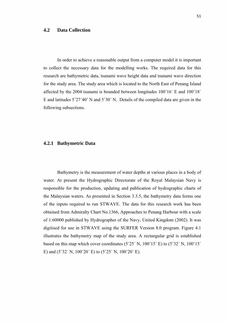
4.2.1 Bathymetric Data

Bathymetry is the measurement of water depths at various places in a body of

water. At present the Hydrographic Directorate of the Royal Malaysian Navy is

responsible for the production, updating and publication of hydrographic charts of

the Malaysian waters. As presented in Section 3.3.5, the bathymetry data forms one

of the inputs required to run STWAVE. The data for this research work has been

obtained from Admiralty Chart No.1366, Approaches to Penang Harbour with a scale

of 1:60000 published by Hydrographer of the Navy, United Kingdom (2002). It was

digitised for use in STWAVE using the SURFER Version 8.0 program. Figure 4.1

illustrates the bathymetry map of the study area. A rectangular grid is established

based on this map which cover coordinates (5˚25΄ N, 100˚15΄ E) to (5˚32΄ N, 100˚15΄

E) and (5˚32΄ N, 100˚20΄ E) to (5˚25΄ N, 100˚20΄ E).

52  

Study Area 

Figure 4.1 Bathymetry Map of Study Area (Source: Admiralty Chart No.1366)

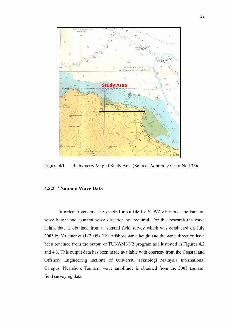
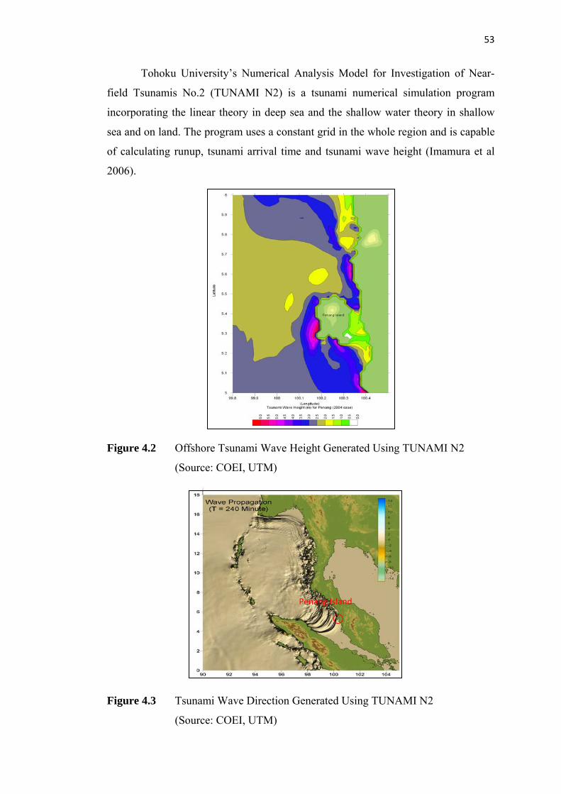
4.2.2 Tsunami Wave Data

In order to generate the spectral input file for STWAVE model the tsunami

wave height and tsunami wave direction are required. For this research the wave

height data is obtained from a tsunami field survey which was conducted on July

2005 by Yalciner et al (2005). The offshore wave height and the wave direction have

been obtained from the output of TUNAMI-N2 program as illustrated in Figures 4.2

and 4.3. This output data has been made available with courtesy from the Coastal and

Offshore Engineering Institute of Universiti Teknologi Malaysia International

Campus. Nearshore Tsunami wave amplitude is obtained from the 2005 tsunami

field surveying data.

53  

Tohoku University’s Numerical Analysis Model for Investigation of Near-

field Tsunamis No.2 (TUNAMI N2) is a tsunami numerical simulation program

incorporating the linear theory in deep sea and the shallow water theory in shallow

sea and on land. The program uses a constant grid in the whole region and is capable

of calculating runup, tsunami arrival time and tsunami wave height (Imamura et al

2006).

Figure 4.2 Offshore Tsunami Wave Height Generated Using TUNAMI N2

(Source: COEI, UTM)

Penang Island

Figure 4.3 Tsunami Wave Direction Generated Using TUNAMI N2

(Source: COEI, UTM)

54  

4.3 Generating Input Files

In order to generate the input files two programs have been applied as

described in following subsections.

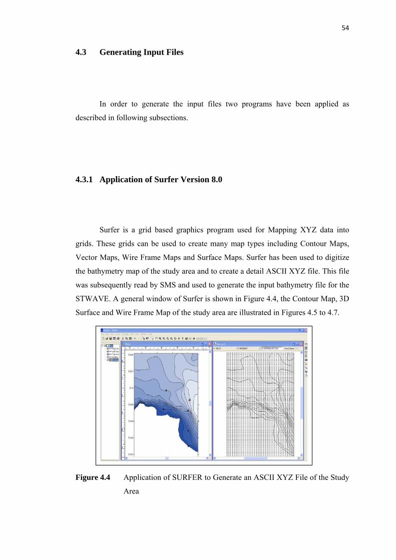
4.3.1 Application of Surfer Version 8.0

Surfer is a grid based graphics program used for Mapping XYZ data into

grids. These grids can be used to create many map types including Contour Maps,

Vector Maps, Wire Frame Maps and Surface Maps. Surfer has been used to digitize

the bathymetry map of the study area and to create a detail ASCII XYZ file. This file

was subsequently read by SMS and used to generate the input bathymetry file for the

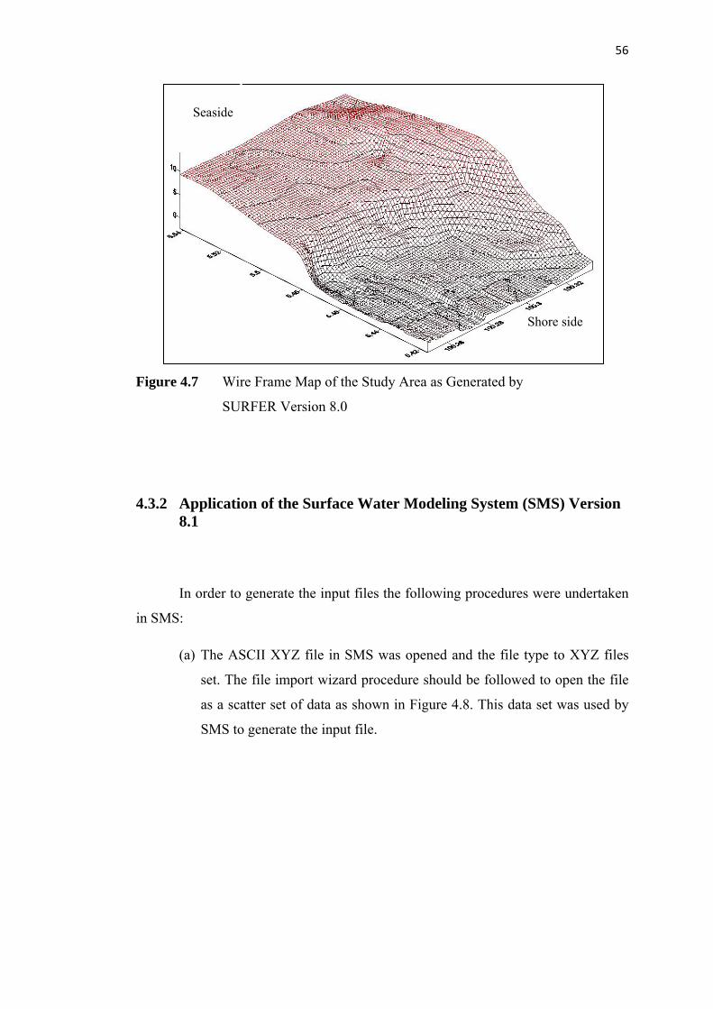
STWAVE. A general window of Surfer is shown in Figure 4.4, the Contour Map, 3D

Surface and Wire Frame Map of the study area are illustrated in Figures 4.5 to 4.7.

Figure 4.4 Application of SURFER to Generate an ASCII XYZ File of the Study

Area

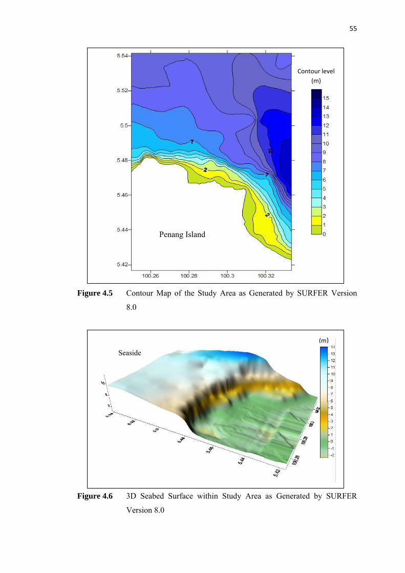
55  

Figure 4.5 Contour Map of the Study Area as Generated by SURFER Version

8.0

(m) 

Seaside

Penang Island

Contour level (m) 

Figure 4.6 3D Seabed Surface within Study Area as Generated by SURFER

Version 8.0

56  

Seaside

Shore side

Figure 4.7 Wire Frame Map of the Study Area as Generated by

SURFER Version 8.0

4.3.2 Application of the Surface Water Modeling System (SMS) Version 8.1

In order to generate the input files the following procedures were undertaken

in SMS:

(a) The ASCII XYZ file in SMS was opened and the file type to XYZ files

set. The file import wizard procedure should be followed to open the file

as a scatter set of data as shown in Figure 4.8. This data set was used by

SMS to generate the input file.

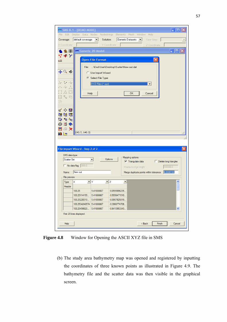
57  

 

Figure 4.8 Window for Opening the ASCII XYZ file in SMS

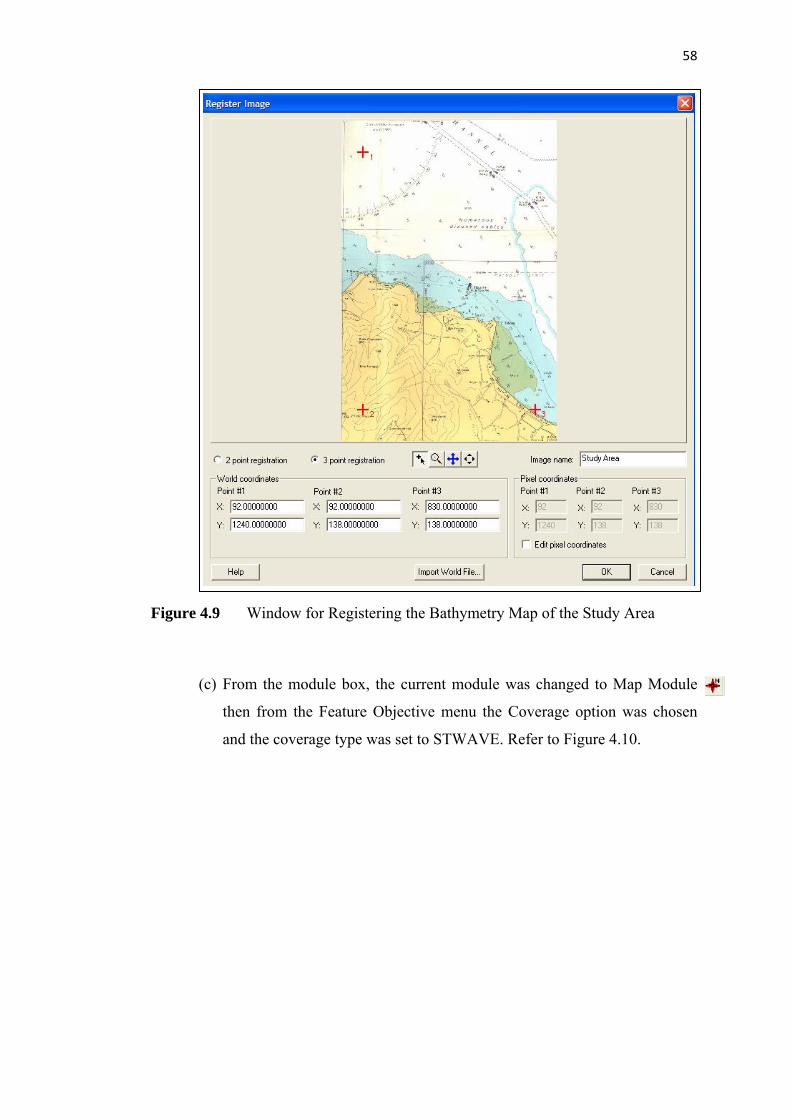
(b) The study area bathymetry map was opened and registered by inputting

the coordinates of three known points as illustrated in Figure 4.9. The

bathymetry file and the scatter data was then visible in the graphical

screen.

58  

Figure 4.9 Window for Registering the Bathymetry Map of the Study Area

(c) From the module box, the current module was changed to Map Module

then from the Feature Objective menu the Coverage option was chosen

and the coverage type was set to STWAVE. Refer to Figure 4.10.

59  

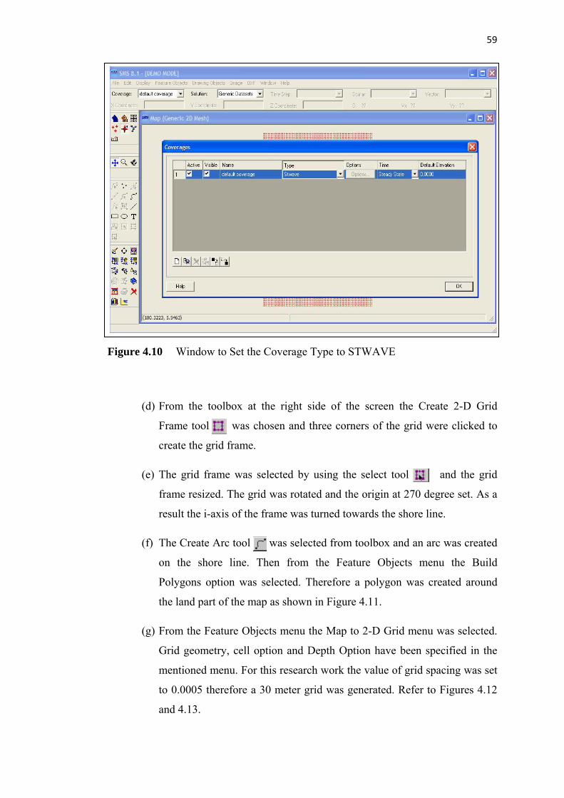
Figure 4.10 Window to Set the Coverage Type to STWAVE

(d) From the toolbox at the right side of the screen the Create 2-D Grid

Frame tool was chosen and three corners of the grid were clicked to

create the grid frame.

(e) The grid frame was selected by using the select tool and the grid

frame resized. The grid was rotated and the origin at 270 degree set. As a

result the i-axis of the frame was turned towards the shore line.

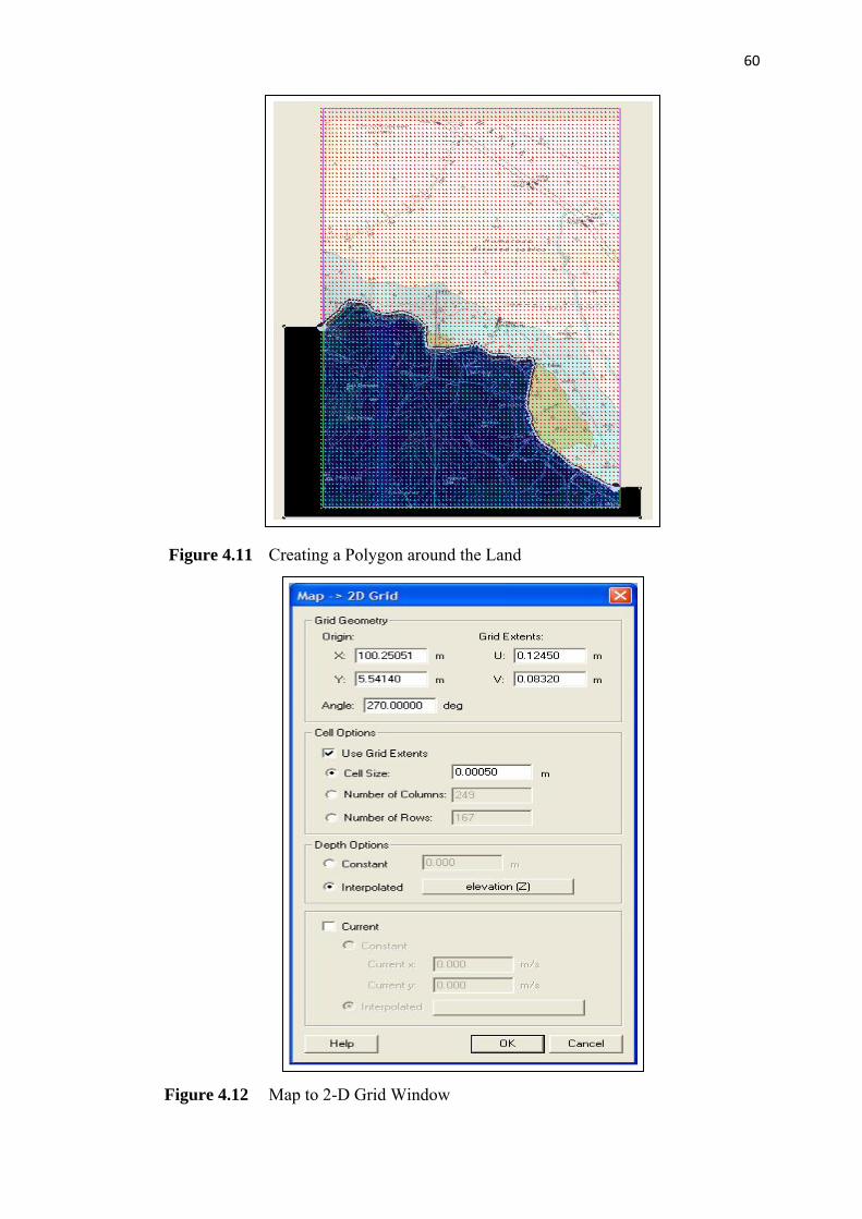
(f) The Create Arc tool was selected from toolbox and an arc was created

on the shore line. Then from the Feature Objects menu the Build

Polygons option was selected. Therefore a polygon was created around

the land part of the map as shown in Figure 4.11.

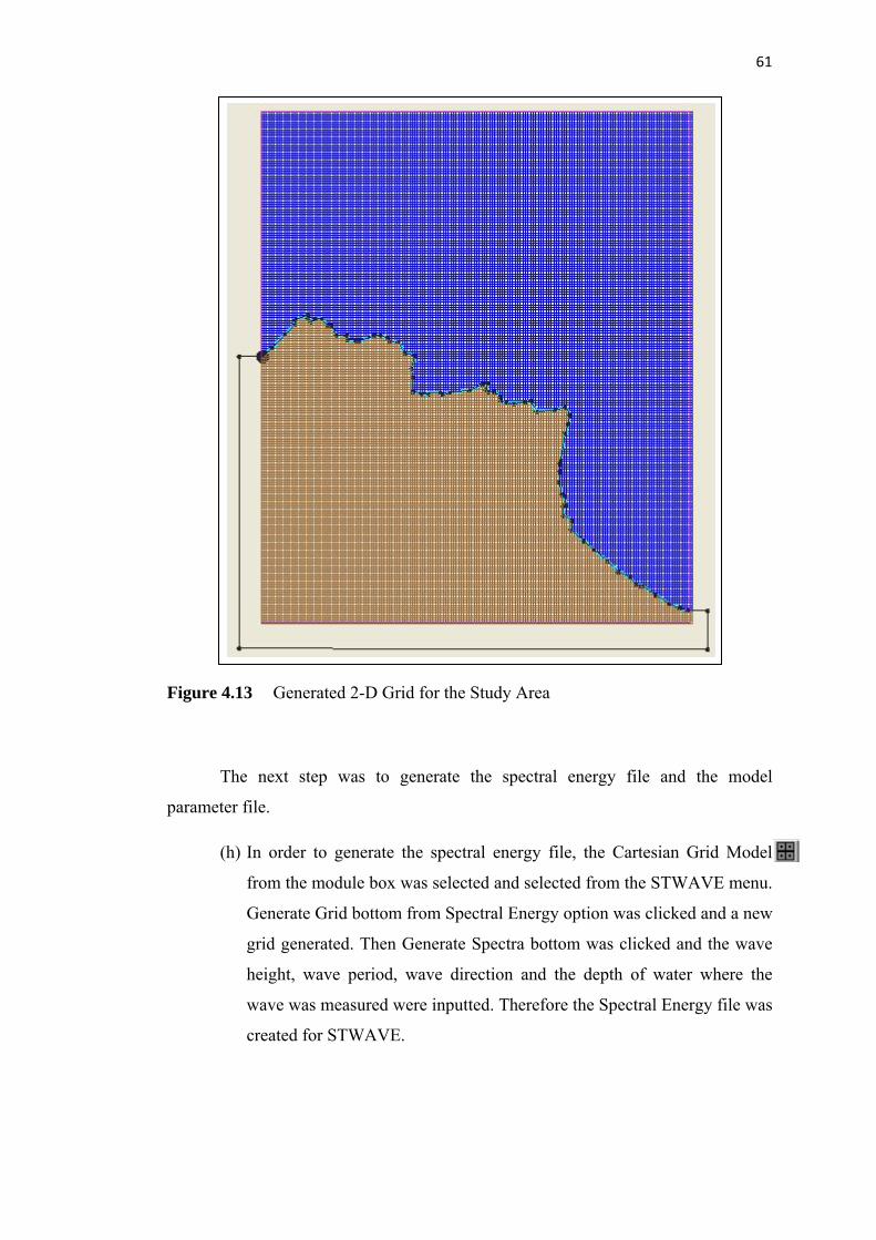
(g) From the Feature Objects menu the Map to 2-D Grid menu was selected.

Grid geometry, cell option and Depth Option have been specified in the

mentioned menu. For this research work the value of grid spacing was set

to 0.0005 therefore a 30 meter grid was generated. Refer to Figures 4.12

and 4.13.

60  

Figure 4.11 Creating a Polygon around the Land

Figure 4.12 Map to 2-D Grid Window

61  

 

Figure 4.13 Generated 2-D Grid for the Study Area

 

The next step was to generate the spectral energy file and the model

parameter file.

(h) In order to generate the spectral energy file, the Cartesian Grid Model

from the module box was selected and selected from the STWAVE menu.

Generate Grid bottom from Spectral Energy option was clicked and a new

grid generated. Then Generate Spectra bottom was clicked and the wave

height, wave period, wave direction and the depth of water where the

wave was measured were inputted. Therefore the Spectral Energy file was

created for STWAVE.

62  

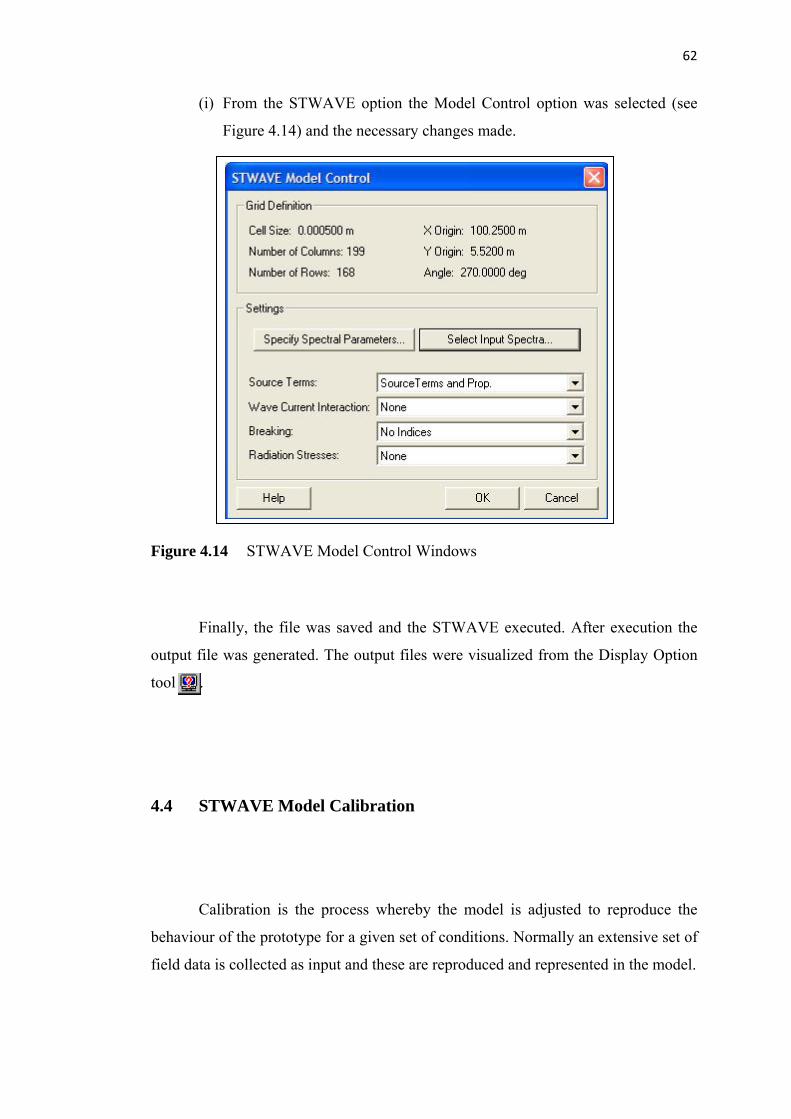
(i) From the STWAVE option the Model Control option was selected (see

Figure 4.14) and the necessary changes made.

Figure 4.14 STWAVE Model Control Windows

Finally, the file was saved and the STWAVE executed. After execution the

output file was generated. The output files were visualized from the Display Option

tool .

4.4 STWAVE Model Calibration

Calibration is the process whereby the model is adjusted to reproduce the

behaviour of the prototype for a given set of conditions. Normally an extensive set of

field data is collected as input and these are reproduced and represented in the model.

63  

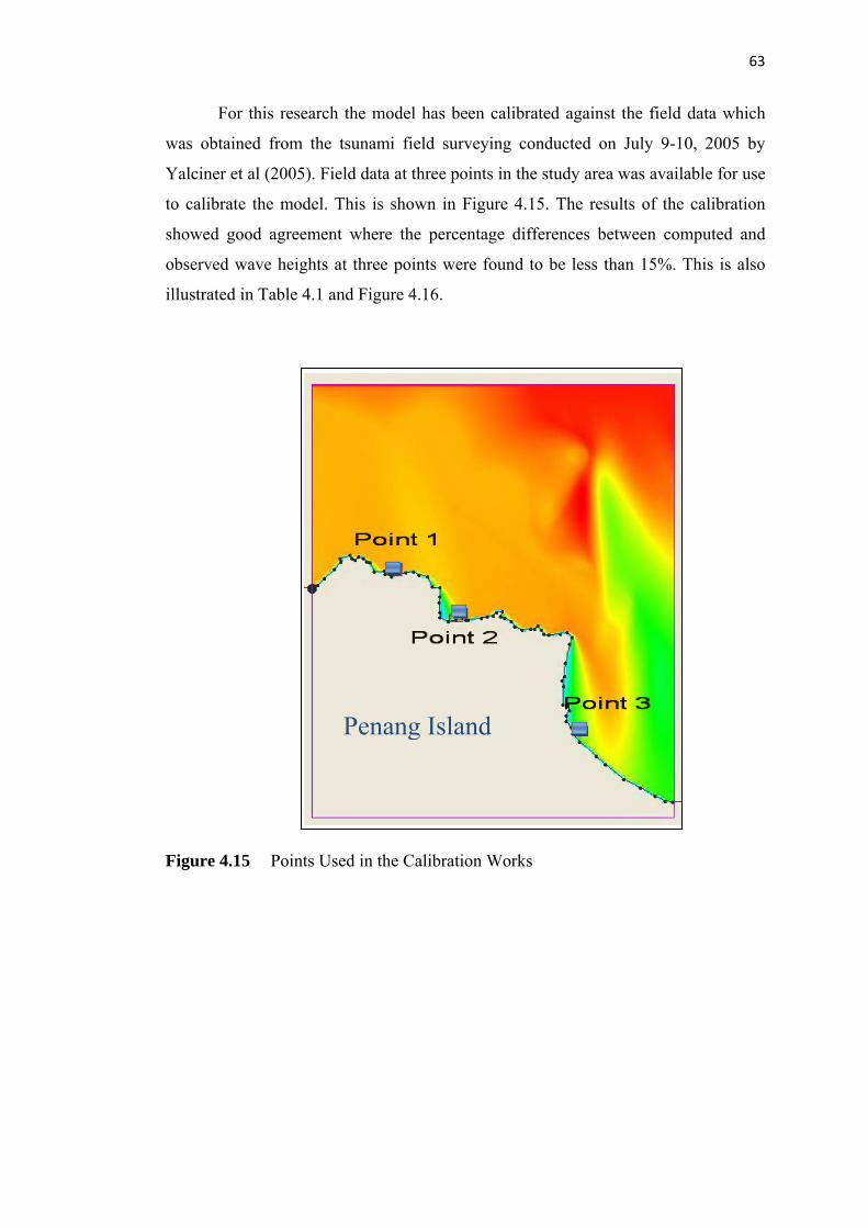
For this research the model has been calibrated against the field data which

was obtained from the tsunami field surveying conducted on July 9-10, 2005 by

Yalciner et al (2005). Field data at three points in the study area was available for use

to calibrate the model. This is shown in Figure 4.15. The results of the calibration

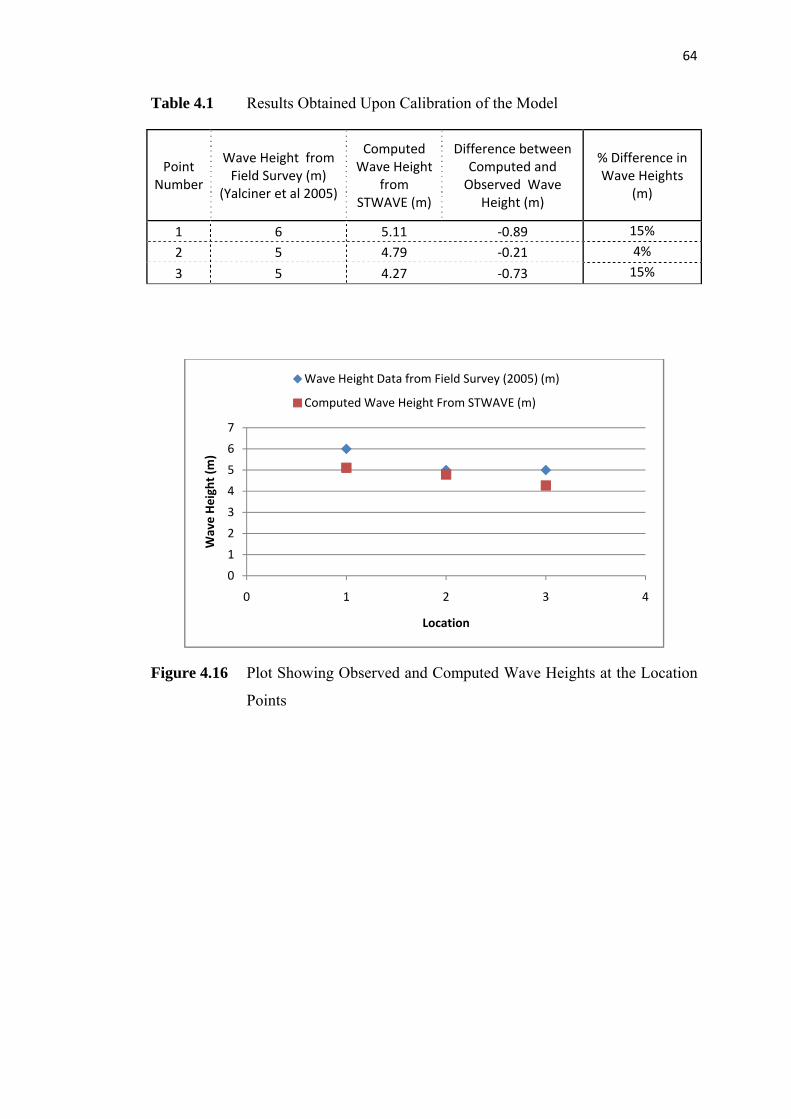
showed good agreement where the percentage differences between computed and

observed wave heights at three points were found to be less than 15%. This is also

illustrated in Table 4.1 and Figure 4.16.

 

Penang Island

Figure 4.15 Points Used in the Calibration Works

64  

Table 4.1 Results Obtained Upon Calibration of the Model

Point Number 

Wave Height  from Field Survey (m) 

(Yalciner et al 2005) 

Computed Wave Height  

from STWAVE (m) 

Difference between Computed and Observed  Wave 

Height (m) 

% Difference in Wave Heights 

(m) 

1  6  5.11  ‐0.89  15% 

2  5  4.79  ‐0.21  4% 

3  5  4.27  ‐0.73  15% 

 

0

1

2

3

4

5

6

7

0 1 2 3

Wave Height (m)

Location

 

4

Wave Height Data from Field Survey (2005) (m)

Computed Wave Height From STWAVE (m)

Figure 4.16 Plot Showing Observed and Computed Wave Heights at the Location

Points

 

 

 

65  

CHAPTER 5

DISCUSSION AND ANALYSIS OF THE COMPUTATIONAL

RESULTS

5.1 Introduction 

As presented earlier in Section 3.3.5, STWAVE is capable of producing five

output files which contained wave spectra at the selected output point; wave height,

direction and period at the selected output points; fields of wave height, period and

direction over the entire STWAVE model domain and fields of radiation stress

gradient over the entire domain.

Amongst these outputs the generated wave height distribution plot is more

significant for use in this research work. The main objective of the present research is

66  

to design an optimised offshore breakwater layout and to determine the wave height

distribution at the lee side of breakwater impacting on the shoreline. Therefore the

procedure employed to determine the optimal layout of the proposed breakwater

which could function to attenuate tsunami wave energy along the North East

coastline of Penang Island is discussed in this chapter.

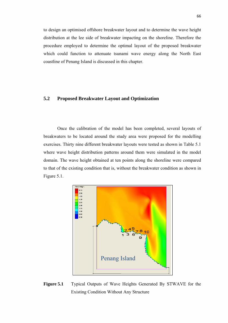
5.2 Proposed Breakwater Layout and Optimization

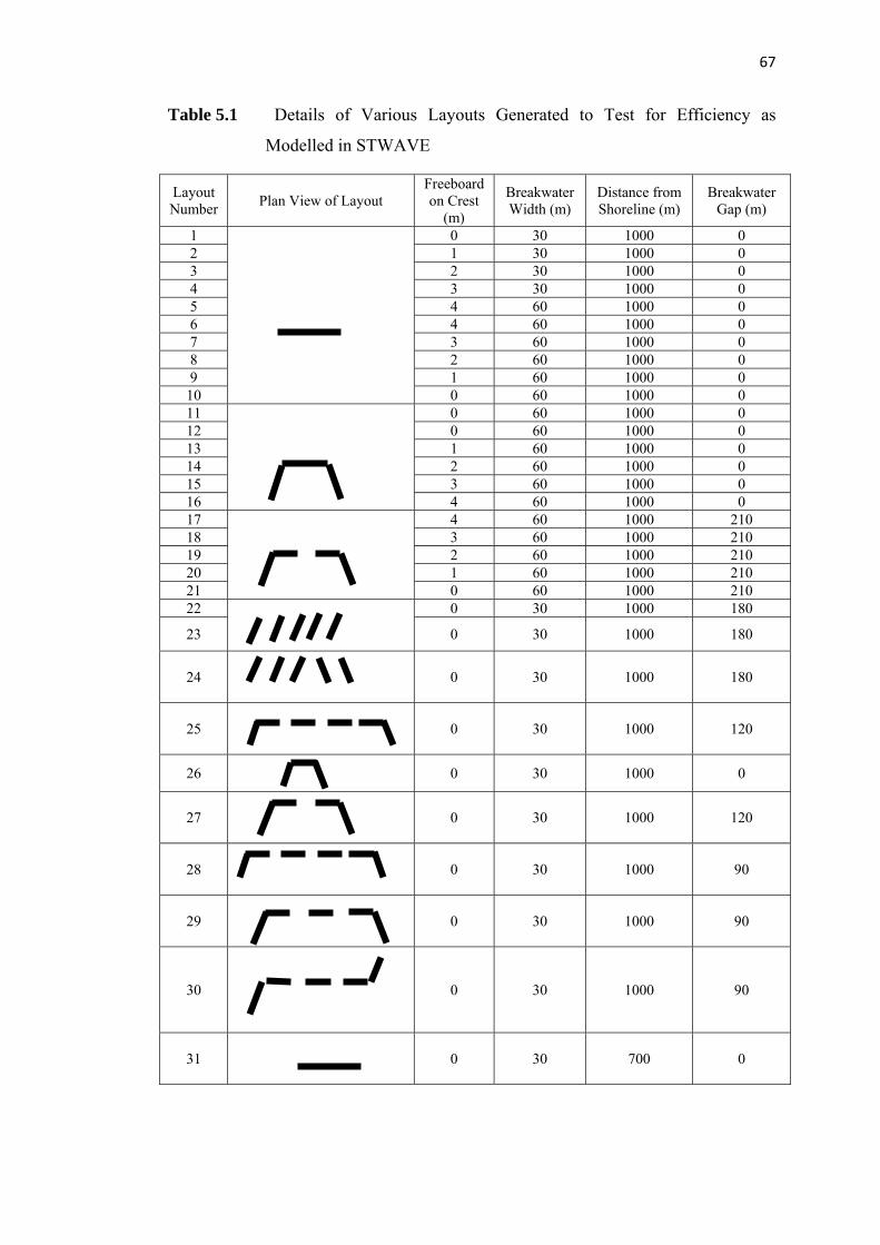
Once the calibration of the model has been completed, several layouts of

breakwaters to be located around the study area were proposed for the modelling

exercises. Thirty nine different breakwater layouts were tested as shown in Table 5.1

where wave height distribution patterns around them were simulated in the model

domain. The wave height obtained at ten points along the shoreline were compared

to that of the existing condition that is, without the breakwater condition as shown in

Figure 5.1.

Penang Island

Figure 5.1 Typical Outputs of Wave Heights Generated By STWAVE for the

Existing Condition Without Any Structure

67  

Table 5.1 Details of Various Layouts Generated to Test for Efficiency as

......................Modelled in STWAVE

Layout Number Plan View of Layout

Freeboard on Crest

(m)

Breakwater Width (m)

Distance from Shoreline (m)

Breakwater Gap (m)

1

0 30 1000 0 2 1 30 1000 0 3 2 30 1000 0 4 3 30 1000 0 5 4 60 1000 0 6 4 60 1000 0 7 3 60 1000 0 8 2 60 1000 0 9 1 60 1000 0

10 0 60 1000 0 11 0 60 1000 0 12 0 60 1000 0 13 1 60 1000 0 14 2 60 1000 0 15 3 60 1000 0 16 4 60 1000 0 17

4 60 1000 210

18 3 60 1000 210 19 2 60 1000 210 20 1 60 1000 210 21 0 60 1000 210 22

0 30 1000 180

23 0 30 1000 180

24

0 30 1000 180

25

0 30 1000 120

26 0 30 1000 0

27

0 30 1000 120

28

0 30 1000 90

29

0 30 1000 90

30

0 30 1000 90

31

0 30 700 0

 

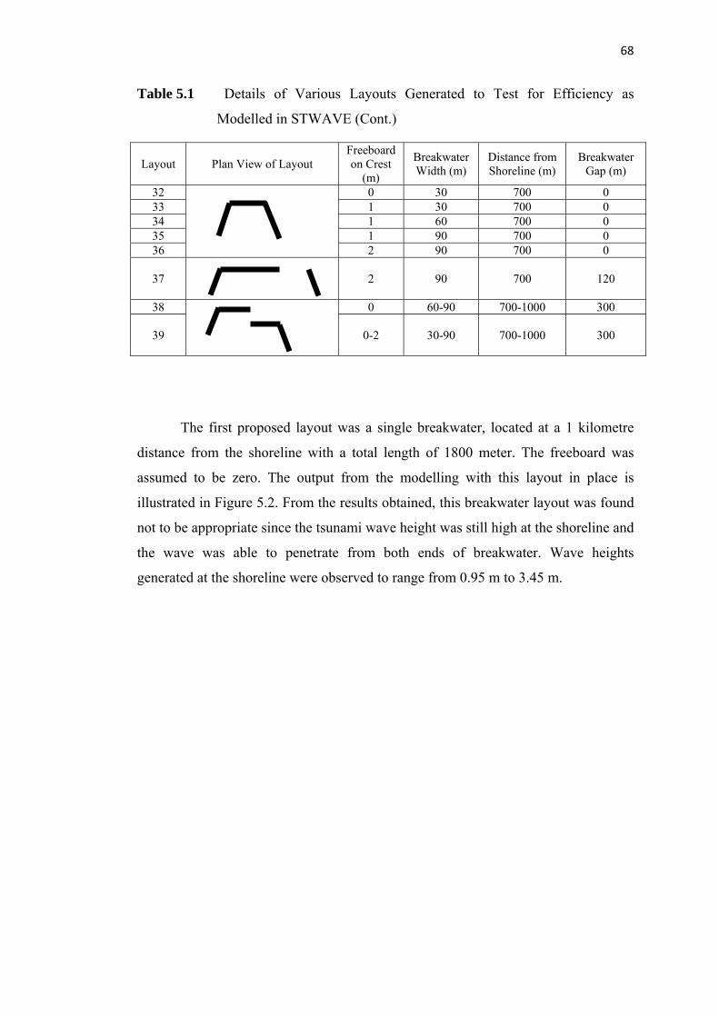
68  

Table 5.1 Details of Various Layouts Generated to Test for Efficiency as

......................Modelled in STWAVE (Cont.)

Layout Plan View of Layout Freeboard on Crest

(m)

Breakwater Width (m)

Distance from Shoreline (m)

Breakwater Gap (m)

32

0 30 700 0 33 1 30 700 0 34 1 60 700 0 35 1 90 700 0 36 2 90 700 0

37

2 90 700 120

38

0 60-90 700-1000 300

39 0-2 30-90 700-1000 300

The first proposed layout was a single breakwater, located at a 1 kilometre

distance from the shoreline with a total length of 1800 meter. The freeboard was

assumed to be zero. The output from the modelling with this layout in place is

illustrated in Figure 5.2. From the results obtained, this breakwater layout was found

not to be appropriate since the tsunami wave height was still high at the shoreline and

the wave was able to penetrate from both ends of breakwater. Wave heights

generated at the shoreline were observed to range from 0.95 m to 3.45 m.

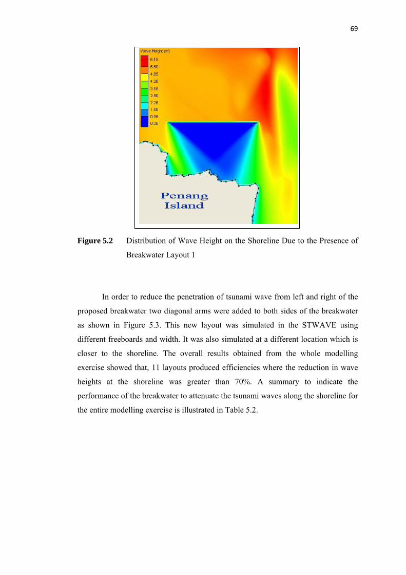
69  

Figure 5.2 Distribution of Wave Height on the Shoreline Due to the Presence of

Breakwater Layout 1

In order to reduce the penetration of tsunami wave from left and right of the

proposed breakwater two diagonal arms were added to both sides of the breakwater

as shown in Figure 5.3. This new layout was simulated in the STWAVE using

different freeboards and width. It was also simulated at a different location which is

closer to the shoreline. The overall results obtained from the whole modelling

exercise showed that, 11 layouts produced efficiencies where the reduction in wave

heights at the shoreline was greater than 70%. A summary to indicate the

performance of the breakwater to attenuate the tsunami waves along the shoreline for

the entire modelling exercise is illustrated in Table 5.2.

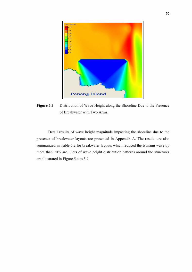
70  

Figure 5.3 Distribution of Wave Height along the Shoreline Due to the Presence

of Breakwater with Two Arms.

Detail results of wave height magnitude impacting the shoreline due to the

presence of breakwater layouts are presented in Appendix A. The results are also

summarized in Table 5.2 for breakwater layouts which reduced the tsunami wave by

more than 70% are. Plots of wave height distribution patterns around the structures

are illustrated in Figure 5.4 to 5.9.

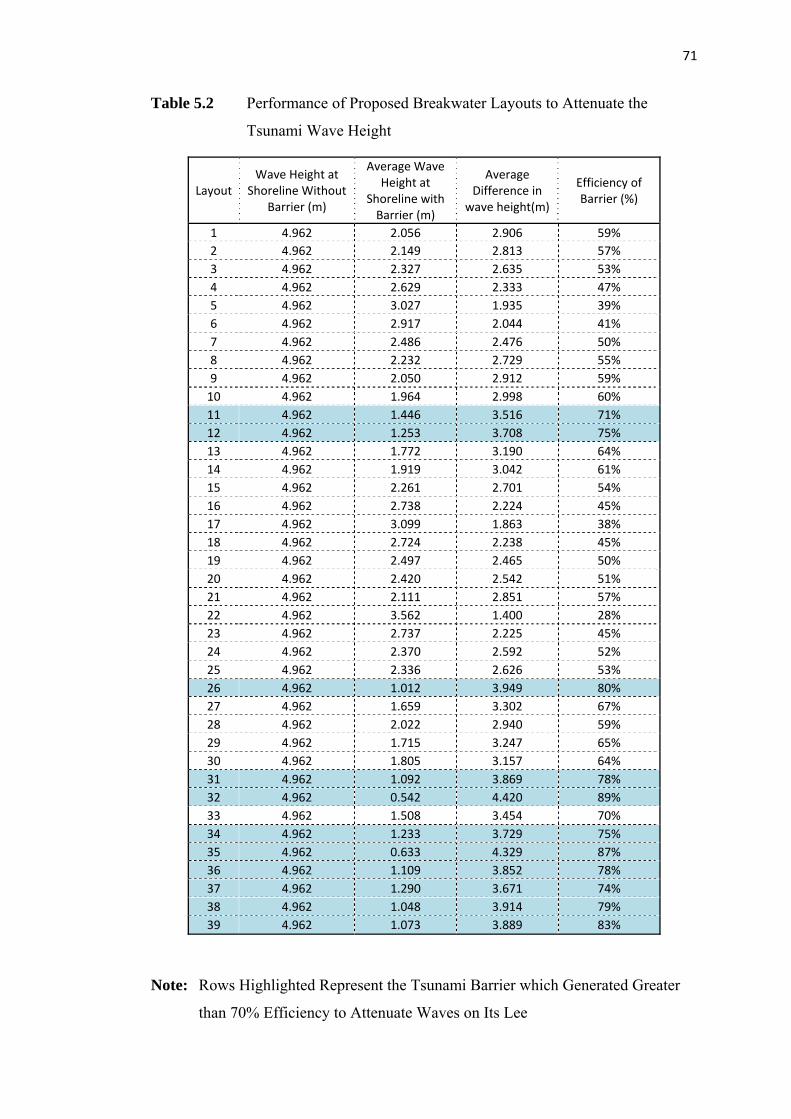
71  

Table 5.2 Performance of Proposed Breakwater Layouts to Attenuate the

Tsunami Wave Height

Layout Wave Height at 

Shoreline Without Barrier (m) 

Average Wave Height at 

Shoreline with Barrier (m) 

Average Difference in 

wave height(m) 

Efficiency of Barrier (%) 

1  4.962  2.056  2.906  59% 2  4.962  2.149  2.813  57% 3  4.962  2.327  2.635  53% 4  4.962  2.629  2.333  47% 5  4.962  3.027  1.935  39% 6  4.962  2.917  2.044  41% 7  4.962  2.486  2.476  50% 8  4.962  2.232  2.729  55% 9  4.962  2.050  2.912  59% 10  4.962  1.964  2.998  60% 11  4.962  1.446  3.516  71% 12  4.962  1.253  3.708  75% 13  4.962  1.772  3.190  64% 14  4.962  1.919  3.042  61% 15  4.962  2.261  2.701  54% 16  4.962  2.738  2.224  45% 17  4.962  3.099  1.863  38% 18  4.962  2.724  2.238  45% 19  4.962  2.497  2.465  50% 20  4.962  2.420  2.542  51% 21  4.962  2.111  2.851  57% 22  4.962  3.562  1.400  28% 23  4.962  2.737  2.225  45% 24  4.962  2.370  2.592  52% 25  4.962  2.336  2.626  53% 26  4.962  1.012  3.949  80% 27  4.962  1.659  3.302  67% 28  4.962  2.022  2.940  59% 29  4.962  1.715  3.247  65% 30  4.962  1.805  3.157  64% 31  4.962  1.092  3.869  78% 32  4.962  0.542  4.420  89% 33  4.962  1.508  3.454  70% 34  4.962  1.233  3.729  75% 35  4.962  0.633  4.329  87% 36  4.962  1.109  3.852  78% 37  4.962  1.290  3.671  74% 38  4.962  1.048  3.914  79% 39  4.962  1.073  3.889  83% 

Note: Rows Highlighted Represent the Tsunami Barrier which Generated Greater

than 70% Efficiency to Attenuate Waves on Its Lee

72  

As shown in Table 5.1, layouts 32 and 35 performed at an efficiency of 89%

and 87% respectively to reduce the tsunami wave height. This also has been

illustrated in Figures 5.4 to 5.9. Breakwater layout 32 was located at 700 meter from

the shoreline and the freeboard was assumed to be zero. Therefore it is visible during

the low tide and cannot preserve the aesthetic value of the area. Moreover, since

there is no gap proposed in this layout, it could affect the self circulation of water

nearshore and has adverse affect on the environment of neighbouring areas. It may

also create problems for any vessel movement in the area during normal conditions.

Layout number 35 was also located at the same position as layout number 32.

The freeboard of this layout was assumed to be one meter but it could also cause

problems for any vessel movement in the area during normal conditions. Besides that

the large crest width (90 meter) of layout 35 may cause this proposal to become less

cost effective.

Even though layouts 32 and 35 performed much better (at an efficiency of

89% and 87% respectively) than layout 39 which only performed at a lower

efficiency of 83%, this layout has been selected to be the most optimal layout. This is

because layout 39 has the advantages given below when compared to the other two

layouts:

a) Segment A with a total length of 1236 m was placed 1 km from the

shoreline in deep water in the model domain. Segment A is a partially

submerged breakwater which is visible during low tide but it is

located away from the shoreline to not affect the aesthetic value of the

shoreline in the study area.

b) Segment B with a total length of 1234 m is nearer to the shoreline

being at 700 meter from shoreline. Since the freeboard is 2 meter

below MSL the breakwater is totally submerged at all times and is not

visible at all during the low tide.

73  

c) A 300 m gap between the two segments allows self circulation of

water. During normal condition this gap may provide a safe passage

for vessels manoeuvring around its lee.

Schematic diagrams of layout 39 are represented in Figures 5.10 to 5.12.

Wave height distribution pattern around the breakwater as generated by STWAVE is

illustrated in Figure 5.13.

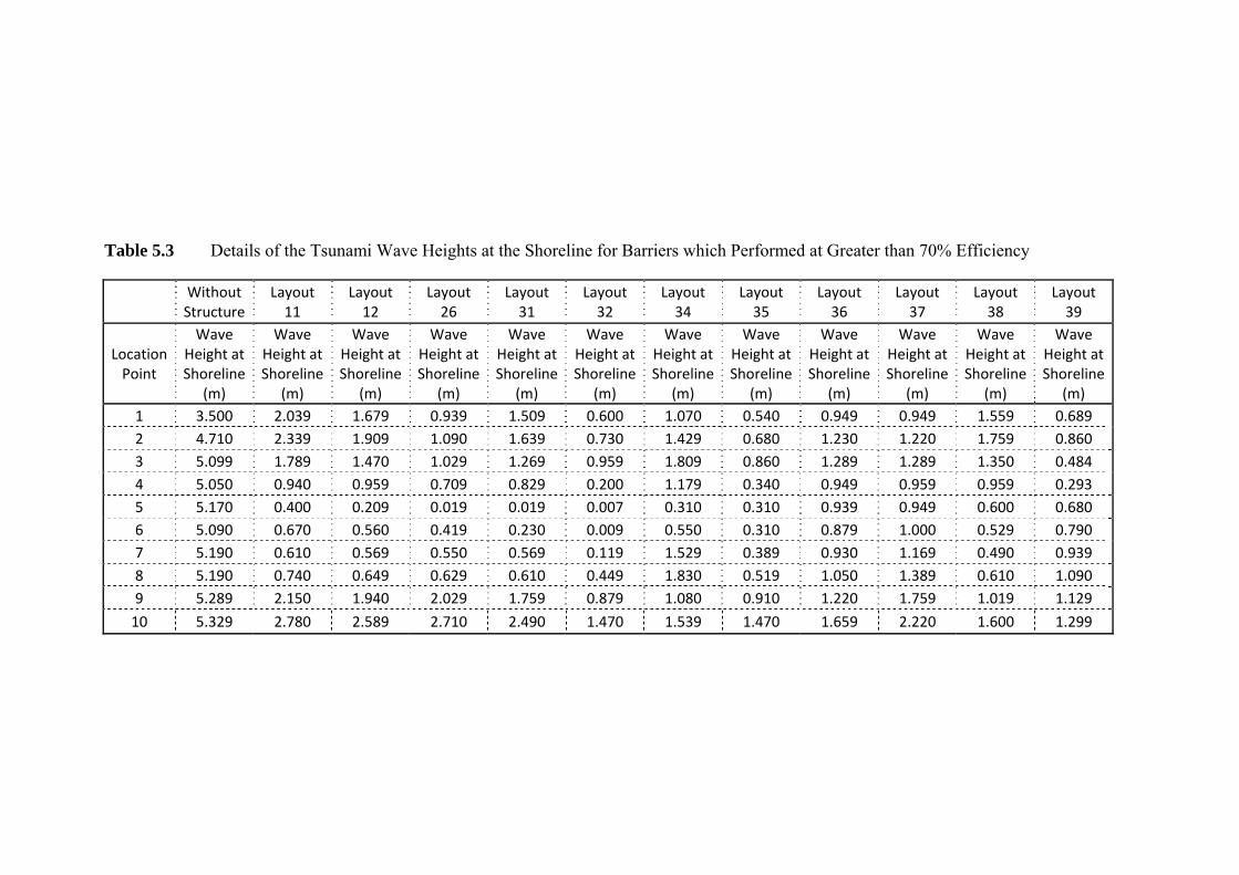
74  

Table 5.3 Details of the Tsunami Wave Heights at the Shoreline for Barriers which Performed at Greater than 70% Efficiency

  Without Structure

Layout 11 

Layout 12 

Layout 26 

Layout 31 

Layout 32 

Layout 34 

Layout 35 

Layout 36 

Layout 37 

Layout 38 

Layout 39 

Location Point  

Wave Height at Shoreline 

(m) 

Wave Height at Shoreline 

(m) 

Wave Height at Shoreline 

(m) 

Wave Height at Shoreline 

(m) 

Wave Height at Shoreline 

(m) 

Wave Height at Shoreline 

(m) 

Wave Height at Shoreline 

(m) 

Wave Height at Shoreline 

(m) 

Wave Height at Shoreline 

(m) 

Wave Height at Shoreline 

(m) 

Wave Height at Shoreline 

(m) 

Wave Height at Shoreline 

(m) 1  3.500  2.039  1.679  0.939  1.509  0.600  1.070  0.540  0.949  0.949  1.559  0.689 2  4.710  2.339  1.909  1.090  1.639  0.730  1.429  0.680  1.230  1.220  1.759  0.860 3  5.099  1.789  1.470  1.029  1.269  0.959  1.809  0.860  1.289  1.289  1.350  0.484 4  5.050  0.940  0.959  0.709  0.829  0.200  1.179  0.340  0.949  0.959  0.959  0.293 5  5.170  0.400  0.209  0.019  0.019  0.007  0.310  0.310  0.939  0.949  0.600  0.680 6  5.090  0.670  0.560  0.419  0.230  0.009  0.550  0.310  0.879  1.000  0.529  0.790 7  5.190  0.610  0.569  0.550  0.569  0.119  1.529  0.389  0.930  1.169  0.490  0.939 8  5.190  0.740  0.649  0.629  0.610  0.449  1.830  0.519  1.050  1.389  0.610  1.090 9  5.289  2.150  1.940  2.029  1.759  0.879  1.080  0.910  1.220  1.759  1.019  1.129 

10  5.329  2.780  2.589  2.710  2.490  1.470  1.539  1.470  1.659  2.220  1.600  1.299 

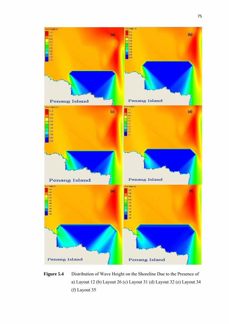
75  

(a) (b)

(c) (d)

(e) (f)

Figure 5.4 Distribution of Wave Height on the Shoreline Due to the Presence of

a) Layout 12 (b) Layout 26 (c) Layout 31 (d) Layout 32 (e) Layout 34

(f) Layout 35

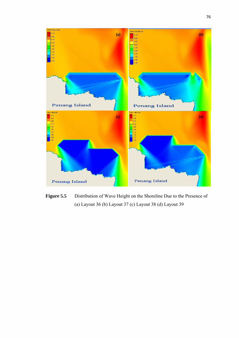
76  

(a) (b)

(c) (d)

Figure 5.5 Distribution of Wave Height on the Shoreline Due to the Presence of

(a) Layout 36 (b) Layout 37 (c) Layout 38 (d) Layout 39

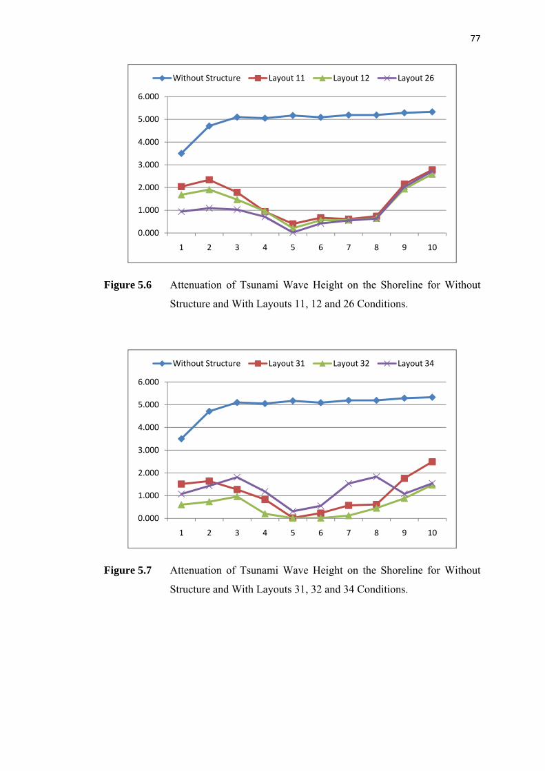
77  

0.000

1.000

2.000

3.000

4.000

5.000

6.000

1 2 3 4 5 6 7 8 9 10

Without Structure Layout 11 Layout 12 Layout 26

Figure 5.6 Attenuation of Tsunami Wave Height on the Shoreline for Without

Structure and With Layouts 11, 12 and 26 Conditions.

0.000

1.000

2.000

3.000

4.000

5.000

6.000

1 2 3 4 5 6 7 8 9 10

Without Structure Layout 31 Layout 32 Layout 34

Figure 5.7 Attenuation of Tsunami Wave Height on the Shoreline for Without

Structure and With Layouts 31, 32 and 34 Conditions.

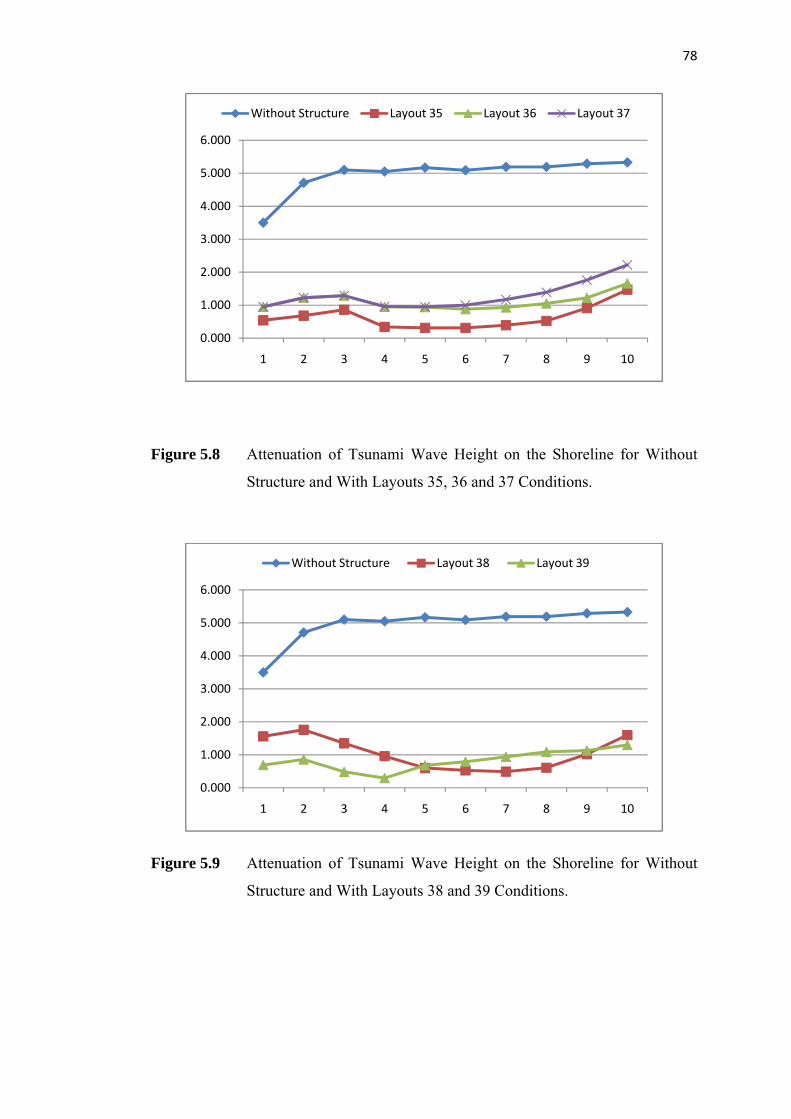
78  

0.000

1.000

2.000

3.000

4.000

5.000

6.000

1 2 3 4 5 6 7 8 9 10

Without Structure Layout 35 Layout 36 Layout 37

Figure 5.8 Attenuation of Tsunami Wave Height on the Shoreline for Without

Structure and With Layouts 35, 36 and 37 Conditions.

0.000

1.000

2.000

3.000

4.000

5.000

6.000

1 2 3 4 5 6 7 8 9 10

Without Structure Layout 38 Layout 39

Figure 5.9 Attenuation of Tsunami Wave Height on the Shoreline for Without

Structure and With Layouts 38 and 39 Conditions.

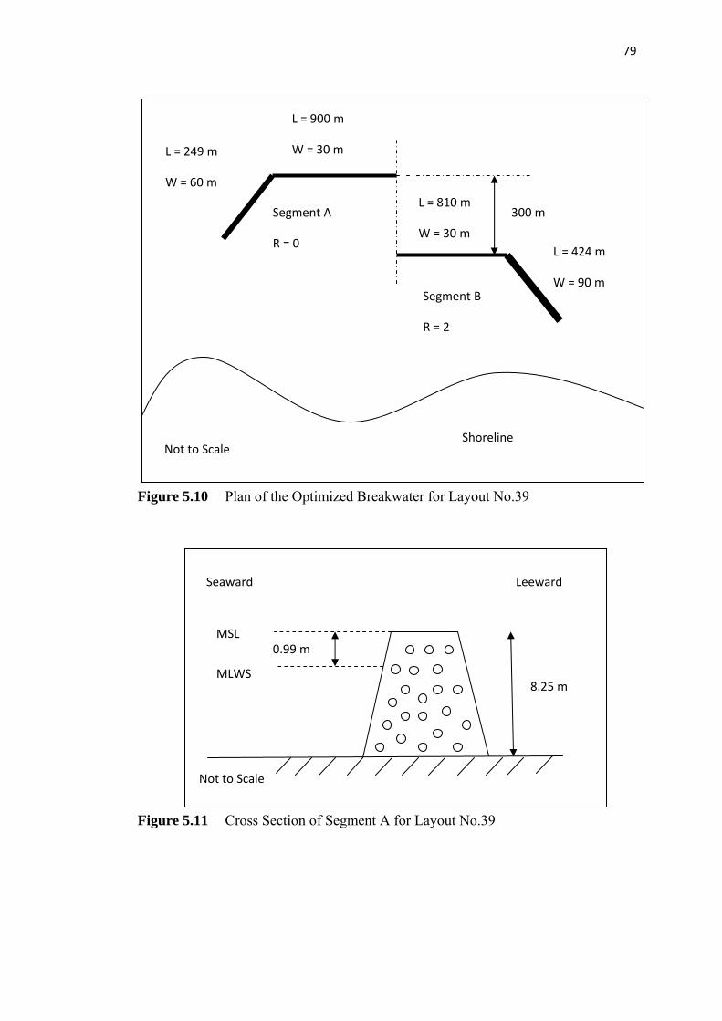
79  

 

 

 

 

 

 

 

Figure 5.10 Plan of the Optimized Breakwater for Layout No.39

 

 

L = 900 m 

W = 30 mL = 249 m 

W = 60 m

L = 810 m 

W = 30 m

Segment A 

R = 0

300 m 

L = 424 m 

W = 90 mSegment B 

R = 2

Shoreline Not to Scale 

Seaward  Leeward 

MSL 

Figure 5.11 Cross Section of Segment A for Layout No.39

8.25 m 

0.99 m

MLWS 

Not to Scale 

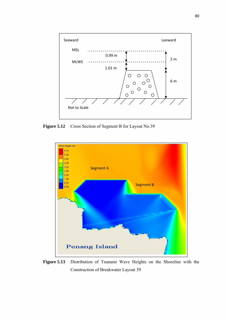
80  

 

  

 

 

 

 

 

 

 

 

Figure 5.12 Cross Section of Segment B for Layout No.39

 

Figure 5.13 Distribution of Tsunami Wave Heights on the Shoreline with the

Construction of Breakwater Layout 39

 

Seaward  Leeward 

MSL 0.99 m   2 m 

MLWS 

1.01 m 

6 m 

Not to Scale 

Segment B 

Segment A 

81  

CHAPTER 6

CONCLUSIONS AND RECOMMENDATIONS

6.1 Conclusions 

The Steady-State Spectral Wave (STWAVE) Module of the Surface Water

Modelling System (SMS) has been applied to simulate the impact of a tsunami wave

when directed towards the north of Penang Island. The model has been calibrated

against field data which was collected during a tsunami field survey by Yalciner et al

(2005) for three points in the study area.

An offshore breakwater has been conceptually designed to dissipate tsunami

wave energy. Thirty nine different layouts have been tested in the STWAVE model in

order to find the most suitable conceptualized layout to construct in the study area.

82  

Eleven layouts showed that an efficiency of greater than 70% was obtained whereby

the breakwaters managed to reduce the tsunami wave heights from a range of 0.6 to

1.5 meter at the shoreline. From the analysis, breakwater layout number 39 has been

selected as the optimized layout in which the breakwater performed to reduce the

tsunami wave height by 83%. Furthermore, it has been selected because layout

number 39 preserved the aesthetic value of the study area and provided sufficient safe

passage for vessel movements to manoeuvre nearshore during the normal conditions.

6.2 Recommendations

The following highlights some of the future works which could be included in

further study:

(a) A finer grid may be applied in order to find the wave height on the

submerged structure and also increase the accuracy of the design.

(b) Hydrodynamic and sediment transport models could be used to evaluate

the response of shoreline and its surroundings due to the effect of

constructing the proposed breakwater.

(c) A 3D numerical model could be utilized to evaluate the effect and

performance of the breakwater when a tsunami wave is directed on the

structure.

(d) Cost estimation and economic analysis could also be undertaken to check

the feasibility of construction of the proposed layout.

83  

LIST OF REFERENCES 

Bardet J.P. et al (2003). Landslide Tsunamis: Recent Findings and Research Directions,

In Bardet J.P. et al (Ed) Landslides Tsunamis: Recent Findings and Research

Directions Switzerland: Birkhauser.

Brigham Young University (2004). Surface Water Modelling System (SMS) Ver.8.1

Tutorial, Environmental Modelling Research Laboratory, Brigham Young

University, USA.

Delft University of Technology (2008). Swan Implementation Manual, Delft University

of Technology, Netherlands

Website: http://www.fluidmechanics.tudelft.nl/swan/index.htm

Demirbilek Z. and Panchang V. (1998). CGWAVE: A Coastal Surface Water Wave

Model of the Mild Slope Equation, Technical Report CHL-98-xx, US Army

Corps of Engineers.

Horikawa K. and Shuto N. (1981). Tsunami Disaster and Protection Measure in Japan,

In Iida K. and Lwasaki T. (Ed) Tsunamis: Their Science and Engineering,

TERRAPUB: Tokyo.

Imamura F. et al (2006). Tsunami Modelling Manual (TUNAMI Model), Tohoku

University, Japan

84  

Komoo I. and Othman M. (2006). The 26.12.04 Tsunami Disaster in Malaysia, an

Environmental, Socio-Economic and Community Well-Being Impact Study,

University Kebangsan Malaysia.

Murty T.S. (2003). Tsunami Wave Height Dependence on Landslide Volume, Pure and

Applied Geophysics, Birkhäuser Basel, 2147-2153.

Pelinovsky E. (2005). Hydrodynamic of Tsunami Waves. In J. Grue and K. Trulsen,

Waves in Geophysical Fluids. USA: Springer Wien New York.

Pencev V. (2004). Interaction of Waves and Reef Breakwaters, In Zimmermann C. et al.

(Eds), Environmental Friendly Coastal Protection, Netherlands: Springer.

Pilarczyk K.W. (2003). Design of Low-Crested (Submerged) Structures-An Overview,

6th International Conference on Coastal and Port Engineering in Developing

Countries, Colombo, Sri Lanka.

Prions P. et al (2004). Low-Crested Structures: Boussinesq Modeling of Waves

Propagation, In Zimmermann C. et al. (Eds), Environmental Friendly Coastal

Protection, Netherlands: Springer.

Segur H. (2006). Waves in Shallow Water, with Emphasis on the Tsunami 2004, In

Anjan Kundu (Ed) Tsunami and Nonlinear Waves, USA: Springer.

Sheppard (2004). EOC 6430 Coastal Structures- Lecture Notes, University of Florida,

Gainsville, USA

Website:http://www.users.coastal.ufl.edu/~sheppard/eco6430main.htm

Shuto N. (2001). Tsunami of Seismic Origin-Science Disaster and Mitigation, In

Yalciner A.C. et al (Eds) Submarine Landslides and Tsunamis, Netherlands:

Kluwer Academic Publishers.

Smith J.M. et al (2001). STWAVE: Steady-State Spectral Wave Model User’s Manual for

STWAVE, Version 3.0, US Army Corps of Engineers®, Engineer Research and

Development Centre.

85  

Todorovska M. I. et al (2001). Near-field Amplitudes of Tsunami from Submarine

Slumps and Slides, In Yalciner A.C. et al. (Eds) Submarine Landslides and

Tsunamis, Netherlands: Kluwer Academic Publishers.

Tokura S. and Ida T. (2005). Simulation of Wave-Dissipating Mechanism on Submerged

Structure Using Fluid-Structure Coupling Capability in LS-DYNA, 5th European

LS-DYNA User Conference.

USACE (2006). Coastal Engineering Manual Part VI: Chapter 2 and Chapter 5,

Coastal and Hydraulic Laboratory, Waterways Experiment Station, Vicksburgh,

USA.

Van der Meer J.W. et al (2005). Wave Transmission and Reflection at Low-Crested

Structures: Design Formulae, Oblique Wave Attack and Spectral Change,

Coastal Engineering 52 (2005) p 915-929.

Van der Plas T. (2007). A Study into the Feasibility of Tsunami Protection Structures for

Banda Aceh and a Preliminary Design of an Offshore Rubblemound Tsunami

Barrier, Master Thesis, Delft University of Technology.

Yalciner A.C. et al (2005). December 26, 2004 Indian Ocean Tsunami Field Survey at

North West Peninsular Malaysia Coast, Penang and Langkawi Islands.

 

86  

 

 

 

 

 

 

 

 

 

APPENDIX A

DETAILS OF THE TSUNAMI WAVE HEIGHTS AT THE

SHORELINE FOR ALL THE PROPOSED LAYOUTS  

 

 

 

 

 

 

 

 

 

 

 

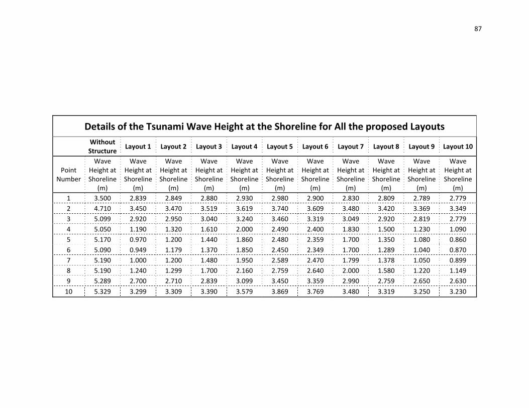
87  

 

 

 

 

Details of the Tsunami Wave Height at the Shoreline for All the proposed Layouts 

 Without Structure 

Layout 1  Layout 2  Layout 3  Layout 4  Layout 5  Layout 6  Layout 7  Layout 8  Layout 9  Layout 10

Point Number 

Wave Height at Shoreline 

(m) 

Wave Height at Shoreline 

(m) 

Wave Height at Shoreline 

(m) 

Wave Height at Shoreline 

(m) 

Wave Height at Shoreline 

(m) 

Wave Height at Shoreline 

(m) 

Wave Height at Shoreline 

(m) 

Wave Height at Shoreline 

(m) 

Wave Height at Shoreline 

(m) 

Wave Height at Shoreline 

(m) 

Wave Height at Shoreline 

(m) 1  3.500  2.839  2.849  2.880  2.930  2.980  2.900  2.830  2.809  2.789  2.779 2  4.710  3.450  3.470  3.519  3.619  3.740  3.609  3.480  3.420  3.369  3.349 3  5.099  2.920  2.950  3.040  3.240  3.460  3.319  3.049  2.920  2.819  2.779 4  5.050  1.190  1.320  1.610  2.000  2.490  2.400  1.830  1.500  1.230  1.090 5  5.170  0.970  1.200  1.440  1.860  2.480  2.359  1.700  1.350  1.080  0.860 6  5.090  0.949  1.179  1.370  1.850  2.450  2.349  1.700  1.289  1.040  0.870 7  5.190  1.000  1.200  1.480  1.950  2.589  2.470  1.799  1.378  1.050  0.899 8  5.190  1.240  1.299  1.700  2.160  2.759  2.640  2.000  1.580  1.220  1.149 9  5.289  2.700  2.710  2.839  3.099  3.450  3.359  2.990  2.759  2.650  2.630 

10  5.329  3.299  3.309  3.390  3.579  3.869  3.769  3.480  3.319  3.250  3.230  

 

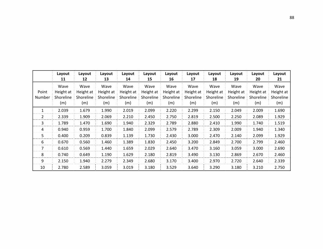
88  

 

 

 

 

 Layout 11 

Layout 12 

Layout 13 

Layout 14 

Layout 15 

Layout 16 

Layout 17 

Layout 18 

Layout 19 

Layout 20 

Layout 21 

Point Number 

Wave Height at Shoreline 

(m) 

Wave Height at Shoreline 

(m) 

Wave Height at Shoreline 

(m) 

Wave Height at Shoreline 

(m) 

Wave Height at Shoreline 

(m) 

Wave Height at Shoreline 

(m) 

Wave Height at Shoreline 

(m) 

Wave Height at Shoreline 

(m) 

Wave Height at Shoreline 

(m) 

Wave Height at Shoreline 

(m) 

Wave Height at Shoreline 

(m) 

1  2.039  1.679  1.990  2.019  2.099  2.220  2.299  2.150  2.049  2.009  1.690 2  2.339  1.909  2.069  2.210  2.450  2.750  2.819  2.500  2.250  2.089  1.929 3  1.789  1.470  1.690  1.940  2.329  2.789  2.880  2.410  1.990  1.740  1.519 4  0.940  0.959  1.700  1.840  2.099  2.579  2.789  2.309  2.009  1.940  1.340 5  0.400  0.209  0.839  1.139  1.730  2.430  3.000  2.470  2.140  2.099  1.929 6  0.670  0.560  1.460  1.389  1.830  2.450  3.200  2.849  2.700  2.799  2.460 7  0.610  0.569  1.440  1.659  2.029  2.640  3.470  3.160  3.059  3.000  2.690 8  0.740  0.649  1.190  1.629  2.180  2.819  3.490  3.130  2.869  2.670  2.460 9  2.150  1.940  2.279  2.349  2.680  3.170  3.400  2.970  2.720  2.640  2.339 

10  2.780  2.589  3.059  3.019  3.180  3.529  3.640  3.290  3.180  3.210  2.750  

 

 

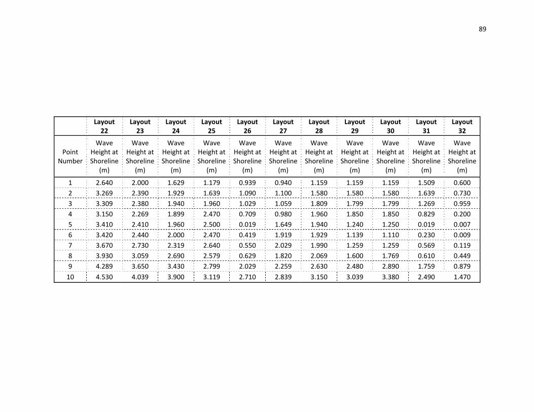
89  

 

 

 

 

 Layout 22 

Layout 23 

Layout 24 

Layout 25 

Layout 26 

Layout 27 

Layout 28 

Layout 29 

Layout 30 

Layout 31 

Layout 32 

Point Number 

Wave Height at Shoreline 

(m) 

Wave Height at Shoreline 

(m) 

Wave Height at Shoreline 

(m) 

Wave Height at Shoreline 

(m) 

Wave Height at Shoreline 

(m) 

Wave Height at Shoreline 

(m) 

Wave Height at Shoreline 

(m) 

Wave Height at Shoreline 

(m) 

Wave Height at Shoreline 

(m) 

Wave Height at Shoreline 

(m) 

Wave Height at Shoreline 

(m) 

1  2.640  2.000  1.629  1.179  0.939  0.940  1.159  1.159  1.159  1.509  0.600 2  3.269  2.390  1.929  1.639  1.090  1.100  1.580  1.580  1.580  1.639  0.730 3  3.309  2.380  1.940  1.960  1.029  1.059  1.809  1.799  1.799  1.269  0.959 4  3.150  2.269  1.899  2.470  0.709  0.980  1.960  1.850  1.850  0.829  0.200 5  3.410  2.410  1.960  2.500  0.019  1.649  1.940  1.240  1.250  0.019  0.007 6  3.420  2.440  2.000  2.470  0.419  1.919  1.929  1.139  1.110  0.230  0.009 7  3.670  2.730  2.319  2.640  0.550  2.029  1.990  1.259  1.259  0.569  0.119 8  3.930  3.059  2.690  2.579  0.629  1.820  2.069  1.600  1.769  0.610  0.449 9  4.289  3.650  3.430  2.799  2.029  2.259  2.630  2.480  2.890  1.759  0.879 

10  4.530  4.039  3.900  3.119  2.710  2.839  3.150  3.039  3.380  2.490  1.470  

 

 

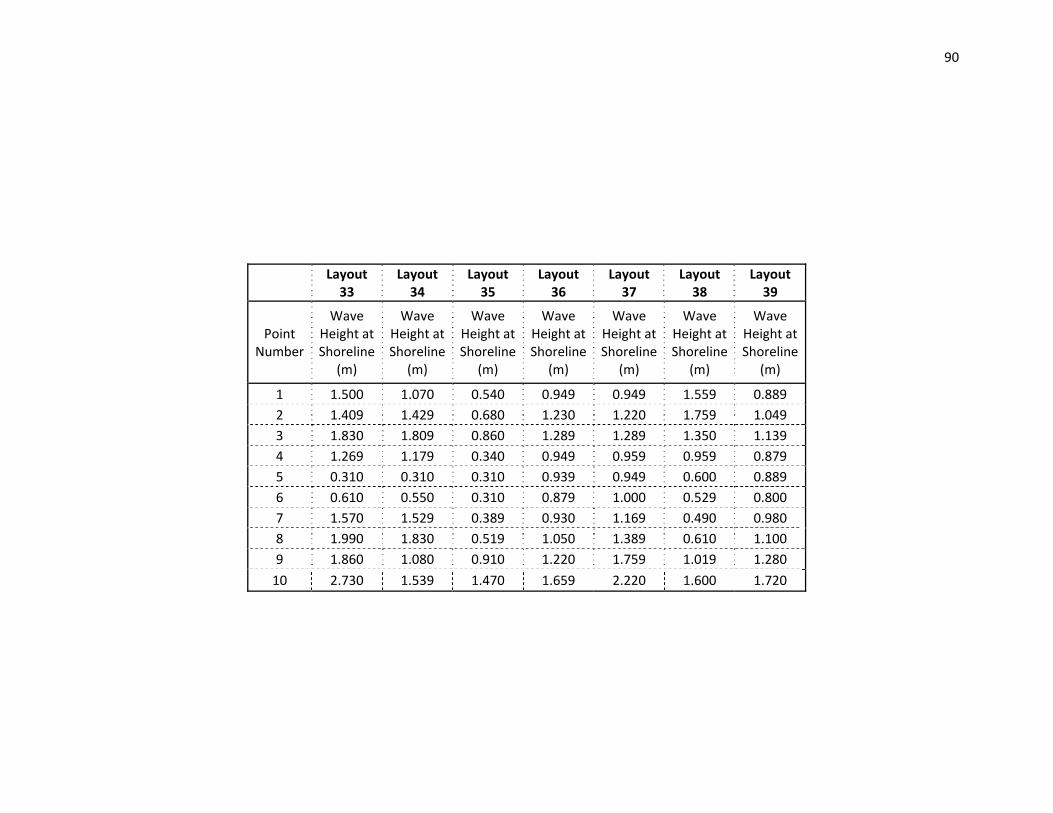
90  

 

 

 

 

 

 Layout 33 

Layout 34 

Layout 35 

Layout 36 

Layout 37 

Layout 38 

Layout 39 

Point Number 

Wave Height at Shoreline 

(m) 

Wave Height at Shoreline 

(m) 

Wave Height at Shoreline 

(m) 

Wave Height at Shoreline 

(m) 

Wave Height at Shoreline 

(m) 

Wave Height at Shoreline 

(m) 

Wave Height at Shoreline 

(m) 

1  1.500  1.070  0.540  0.949  0.949  1.559  0.889 2  1.409  1.429  0.680  1.230  1.220  1.759  1.049 3  1.830  1.809  0.860  1.289  1.289  1.350  1.139 4  1.269  1.179  0.340  0.949  0.959  0.959  0.879 5  0.310  0.310  0.310  0.939  0.949  0.600  0.889 6  0.610  0.550  0.310  0.879  1.000  0.529  0.800 7  1.570  1.529  0.389  0.930  1.169  0.490  0.980 8  1.990  1.830  0.519  1.050  1.389  0.610  1.100 9  1.860  1.080  0.910  1.220  1.759  1.019  1.280 

10  2.730  1.539  1.470  1.659  2.220  1.600  1.720