School of Engineering and Information Technology

ENG460 Engineering Thesis

Design of a Photovoltaic Data Monitoring System and Performance Analysis of the 56 kW the Murdoch

University Library Photovoltaic System

“A report submitted to the School of Engineering and Information Technology, Murdoch

University in partial fulfilment of the requirements for the degree of Bachelor of

Engineering”

2013

Mathew De Cerff

Unit Coordinator: Dr. Gareth Lee

Supervisor: Dr. Martina Calais

ii

Abstract

This paper discusses the design of a data monitoring system, for a PV system which would

enable the calculation of the performance ratio and a.c energy efficiency of a PV system

which the data monitoring system would be installed to. The requirement of this system

was to be at low cost and with reasonable accuracy.

The final design of the data monitoring system consists of a total of five sensors, this

includes a silicon pyranometer, energy meter, module temperature sensor, a.c voltage

sensor and a.c current sensor. The total cost of producing this system was $2002.48.

This paper also discusses the performance analysis of the 56 kW Murdoch University

Photovoltaic System. The time period of this analysis is from June 2011 to August 2013.

It was found that over the 27 month time period of the analysis the total system generation

was 202.67 MWh of electricity. It was seen in January 2013 a peak in monthly out of 10.17

MWh for this month, and it was seen in June 2012 the system production was at its lowest

generating 3.43 MWh. It was established that the sub array which had the best production

was sub array 2 generating a total of 24.48 MWh which is 12.08 % of total production, and

the worst producing sub array was sub array 3 generating a total of 19.97 MWh which is

9.85 % of total production.

The best yield factor month was in January 2013 producing a monthly average of 181.98

kWh/kWp, and the worst yield factor month was June 2012 producing a monthly average of

61.70kWh/kWp. The overall sub array monthly average yield factor for this 27 month period

was 134.47 kWh/kWp, and the poly- crystalline modules and mono- crystalline modules

produced a monthly average yield factor of 139.28 kWh/kWp and 135.77 kWh/kWp,

respectively.

It was established that the performance ratio of the overall system, poly- crystalline

modules and mono- crystalline modules were 0.724, 0.734 and 0.716, respectively. The a.c

energy efficiencies of the overall system, poly- crystalline modules and mono- crystalline

modules were 10.25%, 10.29% and 10.22%, respectively. This shows that the poly-

crystalline modules were the better performing photovoltaic technology.

iii

Acknowledgements

I would like to thank my supervisor Dr Martina Calais for her instrumental guidance and

assistance in my thesis and university studies.

Throughout this project I relied on the guidance of the following individuals:

- Dr David Parlevliet for his assistance is retrieving the data using in this thesis.

- Dr Trevor Pryor for his assistant in converting solar radiation data.

- Jon Lockwood from One Temp for his assistance in the required components needed

in the data monitoring system design.

Finally, I am greatly thankful to Murdoch University and my family and friends for the

continual support throughout my studies.

iv

Contents

Abstract ................................................................................................................................................... ii

Acknowledgements ................................................................................................................................ iii

Figures .................................................................................................................................................... vi

Tables .................................................................................................................................................... vii

1. Introduction .................................................................................................................................... 1

1.1. Project Objectives ................................................................................................................... 2

1.2. Scope of Work ......................................................................................................................... 2

1.3. Literature Review .................................................................................................................... 3

2. Background ..................................................................................................................................... 4

2.1. Murdoch University Photovoltaic System............................................................................... 4

2.1.1. PV Modules ..................................................................................................................... 6

2.1.2. Inverter............................................................................................................................ 7

2.2. Leeming Photovoltaic System ................................................................................................. 7

2.2.1. PV module ....................................................................................................................... 8

2.2.2. Inverter............................................................................................................................ 8

3. Design of Data Monitoring and Data Acquisition System ............................................................... 9

3.1. Requirement Criteria .............................................................................................................. 9

3.2. Selection Criteria ..................................................................................................................... 9

3.3. Design Process and Methodology ......................................................................................... 10

3.3.1. Selection for cost and accuracy comparison ................................................................ 10

3.3.2. Final Selections .............................................................................................................. 13

3.3.3. Design Development ..................................................................................................... 13

3.4. Final DMS Design .................................................................................................................. 14

3.4.1. Solar Radiation Sensor .................................................................................................. 15

3.4.2. Temperature Sensor ..................................................................................................... 15

3.4.3. AC Energy Sensor .......................................................................................................... 16

3.4.4. AC Voltage and Current Sensors ................................................................................... 16

3.4.5. HOBO H22-001 Energy Logger ...................................................................................... 16

3.5. Discussion of the DMS .......................................................................................................... 17

4. Performance Analysis.................................................................................................................... 19

4.1. Performance Analysis Method .............................................................................................. 19

4.1.1. Final Yield ...................................................................................................................... 20

4.1.2. Reference Yield ............................................................................................................. 20

v

4.1.3. Performance Ratio ........................................................................................................ 20

4.1.4. System AC Energy Efficiency ......................................................................................... 21

5. Performance Analysis Results of MULPVS .................................................................................... 22

5.1. Solar Radiation ...................................................................................................................... 22

5.1.1. Method for Solar Radiation Data .................................................................................. 22

5.1.2. Solar Radiation Data Trend ........................................................................................... 23

5.2. System Yields ........................................................................................................................ 26

5.2.1. June to December of 2011 System Yields ..................................................................... 27

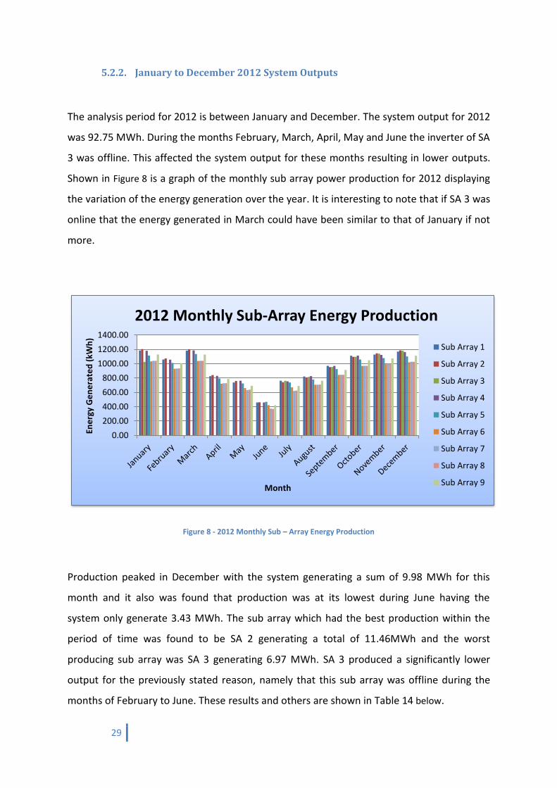
5.2.2. January to December 2012 System Yields .................................................................... 29

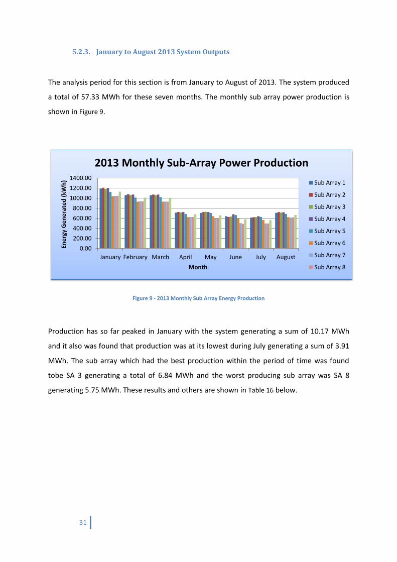
5.2.3. January to August 2013 System Yields .......................................................................... 31

5.2.4. Overall System Yield ...................................................................................................... 33

5.2.5. System Yield Discussion ................................................................................................ 36

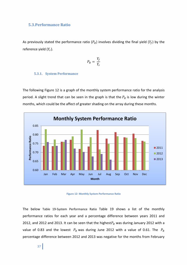
5.3. Performance Ratio ................................................................................................................ 37

5.3.1. System Performance ..................................................................................................... 37

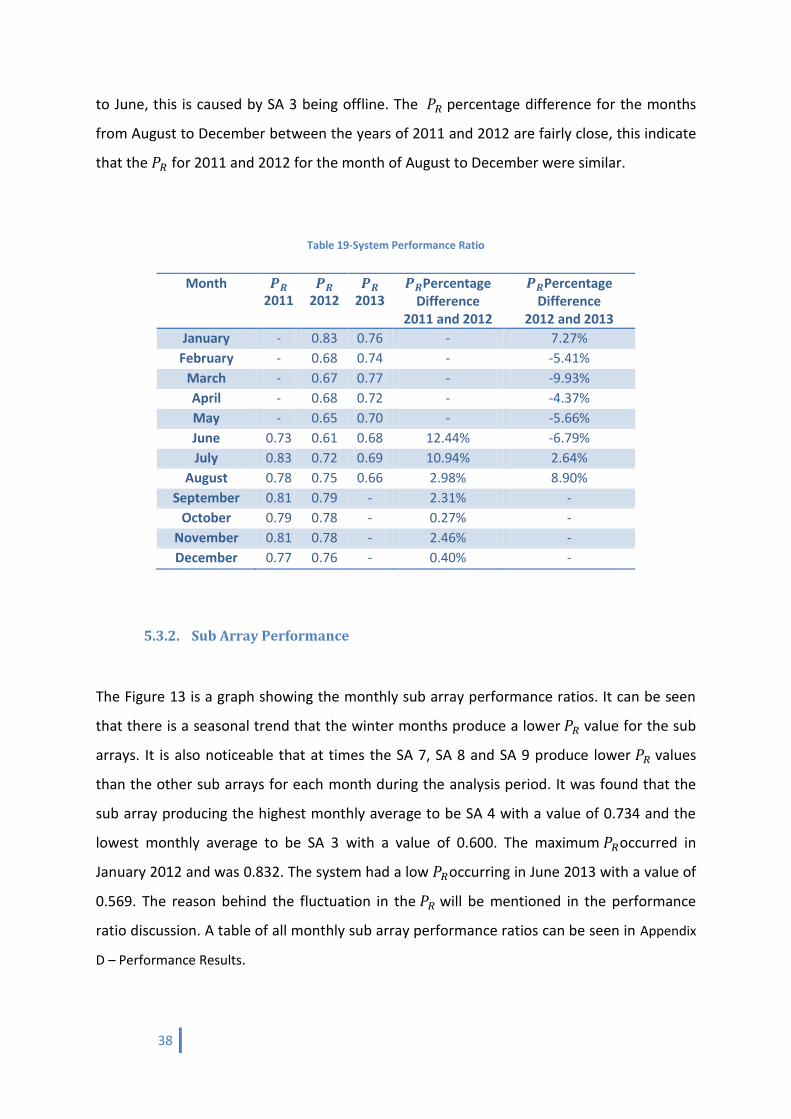
5.3.2. Sub Array Performance ................................................................................................. 38

5.3.3. Performance Ratio Discussion ...................................................................................... 40

5.5. Shading .................................................................................................................................. 40

5.6. System AC Energy Efficiency ................................................................................................. 45

5.7. Comparing PV Technologies ................................................................................................. 46

6. Future Works ................................................................................................................................ 47

7. Conclusion ..................................................................................................................................... 48

8. References .................................................................................................................................... 49

9. Appendix ....................................................................................................................................... 51

Appendix A – Design Specification .................................................................................................... 51

Appendix B – Solar Pathfinder Images .............................................................................................. 51

Appendix C – Sunny SensorBox Data Retrieval ................................................................................. 51

Appendix D – Performance Results .................................................................................................. 51

vi

Figures

Figure 1 - MULPVS Layout (Adapted from Stephen Rose thesis [3]) ...................................................... 5

Figure 2- Leeming PV System .................................................................................................................. 7

Figure 3- Diagram of DMS Design (For the purpose of observing the temperature sensor the

component is place above the array which in actual fact would be under the solar panels.) ............. 15

Figure 4 - Incident Radiation on Plane of Array for Murdoch (Slope: 23°) ........................................... 24

Figure 5 - Monthly Solar Radiation and Monthly System Output over Time ....................................... 25

Figure 6 -Monthly Solar Radiation vs. System AC Energy Efficiency over Time.................................... 26

Figure 7 - 2011 Monthly Sub-Array Energy Production ........................................................................ 27

Figure 8 - 2012 Monthly Sub – Array Energy Production ..................................................................... 29

Figure 9 - 2013 Monthly Sub Array Energy Production ........................................................................ 31

Figure 10 - Overall System Output ........................................................................................................ 33

Figure 11 - Monthly Average Yield Factor per Year (kWh/kWp) .......................................................... 35

Figure 12- Monthly System Performance Ratio .................................................................................... 37

Figure 13 - Monthly Sub Array Performance Ratio ............................................................................... 39

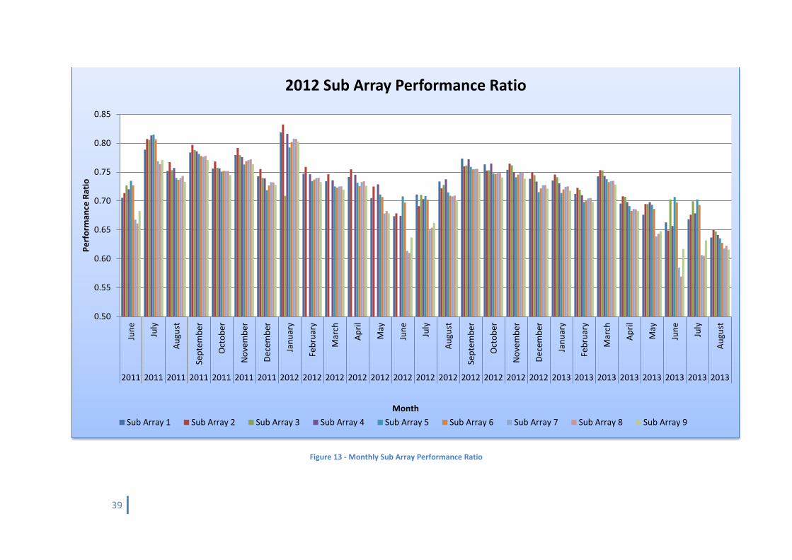
Figure 14 - Shading Effects on Sub Arrays (January) ............................................................................. 41

Figure 15 - Shading Effects on Sub-arrays 1 - 4 Output in June ............................................................ 42

Figure 16 - Shading Effects on Sub-arrays 5 and 6 Output in June ....................................................... 43

Figure 17 - Shading Effects on Sub-arrays 7, 8 and 9 Outputs in June ................................................. 44

vii

Tables

Table 1 - KD135GH-2P Specifications [8] ................................................................................................ 6

Table 2- SG-175M5 Specification [9]....................................................................................................... 6

Table 3- SMA SMC 6000A Specifications [10] ......................................................................................... 7

Table 4 - Sun Rise 190W Specification[11].............................................................................................. 8

Table 5 - SMA SB1100 Specifications[12] ............................................................................................... 8

Table 6 - SMA Webbox Options 1 and 2 ............................................................................................... 11

Table 7- SMA Option 3 .......................................................................................................................... 12

Table 8 - Onset Basic System[13, 19, 20] .............................................................................................. 12

Table 9 - Onset Final System Components[13, 17, 19, 20, 22-24] ........................................................ 14

Table 10 - IEC 61724 Measurement Accuracies [5] .............................................................................. 17

Table 11 - Summary of BoM solar radiation data for the analysis period ............................................ 25

Table 12- 2011 Performance Results .................................................................................................... 28

Table 13 - Sub Array Yield Factors (kWh/kWp) for 2011 ...................................................................... 28

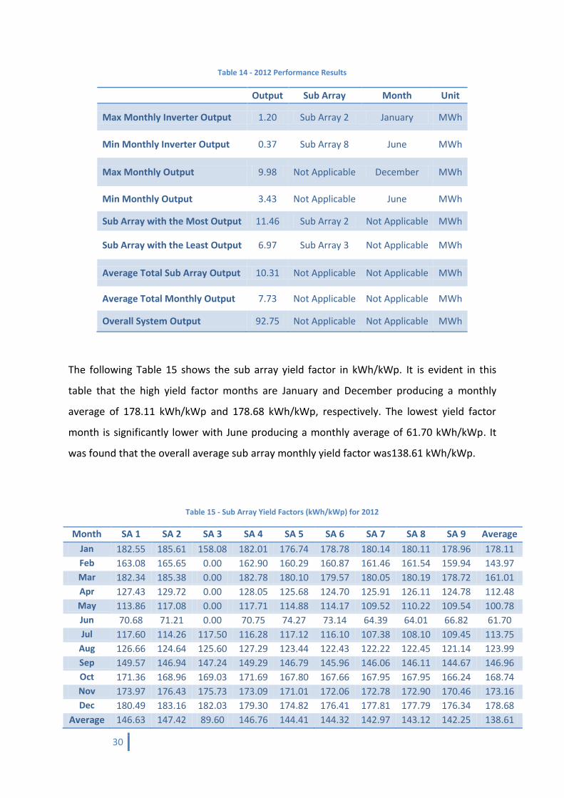
Table 14 - 2012 Performance Results ................................................................................................... 30

Table 15 - Sub Array Yield Factors (kWh/kWp) for 2012 ...................................................................... 30

Table 16 - 2013 Performance Results ................................................................................................... 32

Table 17 - Sub Array Yield Factors (kWh/kWp) for 2013 ...................................................................... 32

Table 18 - Performance Results of the Overall System ......................................................................... 34

Table 19-System Performance Ratio..................................................................................................... 38

Table 20 - Monthly AC Energy Efficiency .............................................................................................. 45

Table 21 - PV Cell Results ...................................................................................................................... 46

1

1. Introduction

Renewable resources accounted for 13.14 % of generation of Australia’s electricity in 2012.

There were 322,000 solar power systems installed nationwide in 2012 and currently there

are a total of over one million solar power systems installed in Australian homes[1].

Murdoch University has a number of renewable energy facilities which include the

Renewable Energy Engineering Lab, Renewable Energy Outdoor Test Area and the

Photovoltaic (PV) training Facility to name a few[2].The university is also producing 56 kW of

solar power into the grid by the Library PV System.

As there has been a rapid growth in PV technology and PV power systems some people

want to know more about their systems and how they are performing. The ability to

optimise the performance of PV systems is becoming more essential as the PV business

becomes more competitive.

The key focus of this thesis involves designing an affordable data monitoring system to be

applied to a residential PV system, in order to review the performance of the system.

Another key focus of this thesis is to complete a performance analysis of a PV system which

involves system yield, performance ratio, and ac energy efficiency, as well as exploring what

factors affects their parameters.

2

1.1. Project Objectives

There were two significant objectives completed within this thesis. The first of these

objectives was to design a data monitoring system (DMS) which had to be installed to a

residential PV system. The DMS had to have the ability to determine the performance ratio

and a.c energy efficiency of the system, at low cost, whilst being reasonably accurate and

being independent of the inverter.

The second main object was to complete a performance analysis on the Murdoch University

Library Photovoltaic System (MULPVS). The analysis parameters of this PV system include

the system and sub array yields, performance ratios, a.c energy efficiency, PV cell

technology comparison and shading effects.

1.2. Scope of Work

There are many tasks involved in this thesis project which allow the main objectives to be

achieved. These are as follows:

1. Research data monitoring systems

2. Design a data monitoring system which meets the design requirements

3. Liaise with Sales Engineers to acquire quotations

4. Arrange equipment for data monitoring system

5. Sensor positioning investigation relating to the solar radiation sensor

6. Data retrieval of MULPVS and documentation of this process

7. Performance analysis of the MULPVS

3

1.3. Literature Review

To gain an initial understanding of what a thesis entailed and what to include in this project,

the reading of two theses was completed. These theses were by Stephen Rose and by Mael

Riou titled ‘Performance evaluation, simulation and design assessment of the 56kWp

Murdoch University Library photovoltaic system’ [3]and ‘Monitoring and data acquisition

system for the photovoltaic training facility on the engineering and energy building’

[4]respectively.

The basis of the performance analysis completed in this paper was a continuation from S.

Rose’s thesis. The performance analysis also refers to IEC 61724 ‘Photovoltaic system

performance monitoring – Guidelines for measurement, data exchange and analysis’[5] and

also explores the ideas raised in the paper by David L. King ‘More efficient methods for

specifying and monitoring PV system performance’[6].

The design of the data monitoring system also refers to the paper by D.L. King and the IEC

61724. Other literature which was used included ‘SMA’ and ‘Oneset’ websites exploring the

different possible technologies to be used in the data monitoring system.

4

2. Background

2.1. Murdoch University Photovoltaic System

As apart the Murdoch University’s Environmental Sustainability Program 15% of electricity

at the university was to be produced from renewable energy resources[7]. In order for this

to become a possibility, the university installed a 56 kW photovoltaic (PV) system. The

installation of the Murdoch University Library Photovoltaic System (MULPVS) was

completed in two stages.

The first stage instalment consisted of 192 x 135 W Kyocera poly- crystalline (poly- Si) PV

panels. The size of this installation produced a peak rated power output of 26 kW. Included

in the instalment were four SMA SMC 6000A inverters. The system was installed by Solar

Unlimited and was completed in 2008.

The second instalment occurred in 2009 and consisted of an addition of 171 x 175 W Sun

Grid mono- crystalline PV panels. Again, SMA MC 6000A inverters were used and an

additional 5 inverters were added to the system. This instalment produces a peak rated

power output of 30 kW. The system was installed by Solar PV.

The layout of this system is made up of 9 sub arrays. Sub arrays 1 to 4 are made up of two

parallel strings with 24 panels in each string with a peak output of 6.48 kW, sub arrays 5 and

9 are made up of three parallel strings with 12 panels in each string with a peak output of

6.3 kW and sub arrays 6, 7 and 8 are made up of three parallel strings with 11 panels in each

string with a peak output of 5.775 kW. The following Figure 1shows a schematic diagram of

the layout, displays the locations of each sub array.

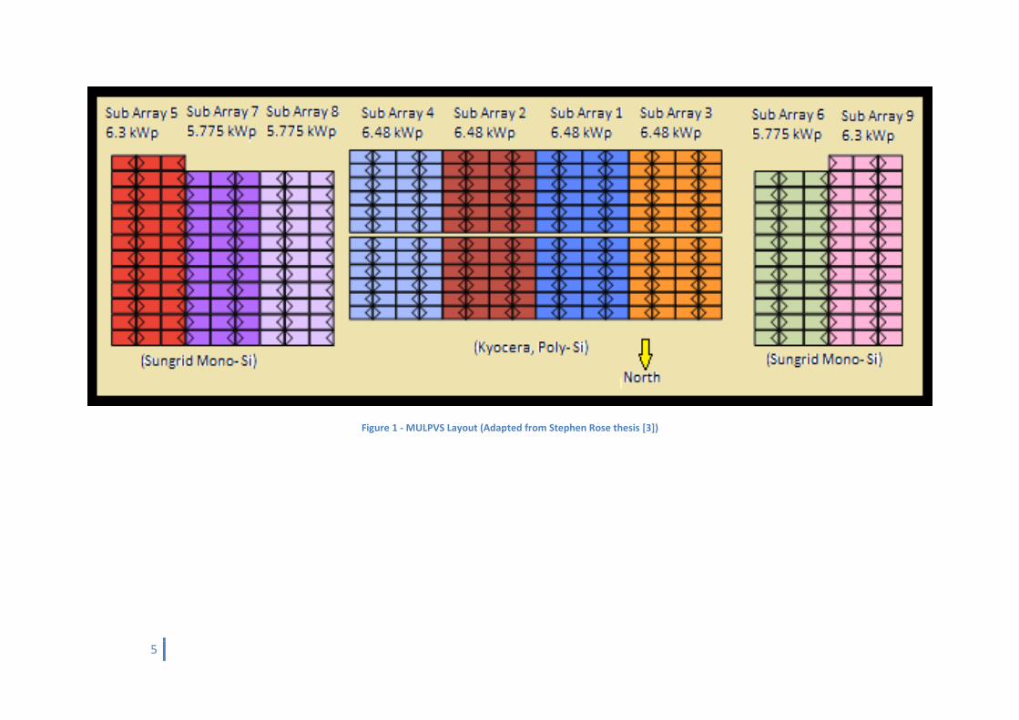
5

Figure 1 - MULPVS Layout (Adapted from Stephen Rose thesis [3])

6

2.1.1. PV Modules

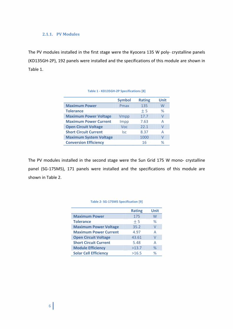
The PV modules installed in the first stage were the Kyocera 135 W poly- crystalline panels

(KD135GH-2P), 192 panels were installed and the specifications of this module are shown in

Table 1.

Table 1 - KD135GH-2P Specifications [8]

Symbol Rating Unit

Maximum Power Pmax 135 W Tolerance 5 % Maximum Power Voltage Vmpp 17.7 V Maximum Power Current Impp 7.63 A Open Circuit Voltage Voc 22.1 V Short Circuit Current Isc 8.37 A Maximum System Voltage 1000 V Conversion Efficiency 16 %

The PV modules installed in the second stage were the Sun Grid 175 W mono- crystalline

panel (SG-175M5), 171 panels were installed and the specifications of this module are

shown in Table 2.

Table 2- SG-175M5 Specification [9]

Rating Unit

Maximum Power 175 W Tolerance 5 % Maximum Power Voltage 35.2 V Maximum Power Current 4.97 A Open Circuit Voltage 43.61 V Short Circuit Current 5.48 A Module Efficiency >13.7 % Solar Cell Efficiency >16.5 %

7

2.1.2. Inverter

The inverter used in all nine sub arrays is the SMA Sunny mini Central 6000A inverter. The

specifications for this inverter can be seen in the following Table 3.

Table 3- SMA SMC 6000A Specifications [10]

Rating Unit

Maximum DC Input Power 6300 W Maximum DC Voltage 600 V PV Voltage rage, MPPT 246 – 480 V Maximum Input Current 26 A Nominal AC Output Power 6000 W Maximum AC Output Power 6000 W Maximum Output Current 26 A Maximum Efficiency 96.1 %

2.2. Leeming Photovoltaic System

The PV system which the data monitoring system (DMS) is applied to is located at Dr

Martina Calais’ residence. For the purpose of this report this system is referred to as the

Leeming PV System (LPVS). This system is a 1.1 kW system which includes 7 Sun Rise 190 W

mono- crystalline panels along with a SMA SB1100 inverter. The image shown in Figure 2 is

the LPVS.

Figure 2- Leeming PV System

8

2.2.1. PV module

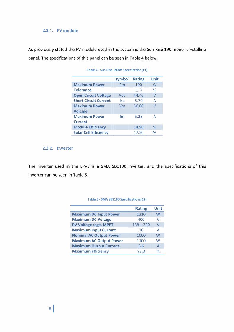
As previously stated the PV module used in the system is the Sun Rise 190 mono- crystalline

panel. The specifications of this panel can be seen in Table 4 below.

Table 4 - Sun Rise 190W Specification[11]

symbol Rating Unit

Maximum Power Pm 190 W Tolerance 3 % Open Circuit Voltage Voc 44.46 V Short Circuit Current Isc 5.70 A Maximum Power Voltage

Vm 36.00 V

Maximum Power Current

Im 5.28 A

Module Efficiency 14.90 % Solar Cell Efficiency 17.50 %

2.2.2. Inverter

The inverter used in the LPVS is a SMA SB1100 inverter, and the specifications of this

inverter can be seen in Table 5.

Table 5 - SMA SB1100 Specifications[12]

Rating Unit

Maximum DC Input Power 1210 W Maximum DC Voltage 400 V PV Voltage rage, MPPT 139 – 320 V Maximum Input Current 10 A Nominal AC Output Power 1000 W Maximum AC Output Power 1100 W Maximum Output Current 5.6 A Maximum Efficiency 93.0 %

9

3. Design of Data Monitoring and Data Acquisition System

3.1. Requirement Criteria

A major requirement of this project was to implement the design of a Data Monitoring

System (DMS). This DMS was to be a basic system which would monitor the LPVS. The

purpose of the monitoring system was to carry out a performance assessment of the LPVS.

In the paper “More efficient methods for specifying and monitoring PV system

performance” by David L. King, it suggests that a.c energy efficiency is an advantageous way

to analyse a PV system [6]. This was done because a basic monitoring system would be

needed, which would include solar radiation and a.c energy output sensors.

The DMS was to include a data logger, solar radiation sensor and an energy (kWh) sensor at

minimum. The solar radiation and energy measured are the only parameters necessary for

the calculation of the system’s a.c energy efficiency. Other requirements were that the

DMS was to be a low cost system and it was suggested that international standard IEC

61724 ‘Photovoltaic system performance monitoring – Guidelines for measurement, data

exchange and analysis’ should be referred to during the design[5].

3.2. Selection Criteria

The sensors for the DMS were selected on the basis of a combination of cost and accuracy.

On this note, a number of components were looked into and tables were produced which

outline the cost and accuracy of the components. These tables were used to help select the

most appropriate option for this system.

10

3.3. Design Process and Methodology

The design process was extensive and involved research and communication with suppliers

and supervisor Martina Calais. The first step for this process was to explore a range of

different possible technologies to select from. From the research it was found there were a

few possibilities for the design development of the DMS. This includes SMA technology,

Onset HOBO Data Loggers, Data Taker, Campbell Scientific Australia and Unidata. From the

research it was quickly evident that some technologies would be expensive, so the two main

equipment preferences were the SMA technology and Onset HOBO Data Loggers. After

narrowing down the companies to design the system, feasible design options were

developed to be analysed and compared against each other.

3.3.1. Selection for cost and accuracy comparison

As previously stated the two main design options which were to be considered were the

SMA technology or the HOBO data logger technology. The following sections explore the

process for final selection.

3.3.1.1. SMA Technology

Research into SMA technology was conducted and the components needed to be

compatible with the SMA SB1100 inverter. There were a number of components which were

possible options for the design which are shown in Table 6 and Table 7.

11

Table 6 - SMA Webbox Options 1 and 2

SMA Option

Component Accuracy (%)

Cost ($) Total Cost ($)

Option 1

SMA Sunny Sensorbox ±8 517

1312

SMA- Sunny Webbox Bluetooth Not specified

660

Inverter communication card Not Specified

$135

Sunny Portal Not Specified

Free website

Option 2

SMA Sunny Sensorbox ±8 517

1334

SMA-Sunny Webbox + RS485 interface cable

Not Specified

682

Inverter communication card Not Specified

$135

Sunny Portal Not Specified

Free website

Both designs shown in Table 6 include a SMA Sunny Sensorbox which is a component that

can measure solar radiation, wind speed, ambient temperature and module

temperature[13].They also include a Sunny Webbox which is a communication device, one

of these devices communicates via Bluetooth and no cables are needed while the other

communicates using cable connecting to the communication card[14, 15]. Both these

devices communicate with the PV inverter and collect all the data which is then transmitted

to the Sunny Portal. Sunny Portal is a website that stores and manages all the data and is

accessed via the internet, via PC’s or mobile phones. There are reporting functions within

Sunny Portal which provide regular updates via e-mail[16].

It was found that the use of a Sunny Webbox was not the only way to communicate with the

SMA SB1100 inverter. A SMA Bluetooth Piggy-Back card can be installed directly to the

inverter and from this device it can be communicated via Bluetooth to the Sunny Explorer

where all the data can be collected. Sunny Explorer is a free program which can be

downloaded from the SMA website[17, 18].

12

Table 7- SMA Option 3

SMA Option Component Accuracy (%) Cost ($) Total Cost ($)

Option 3 SMA Bluetooth Piggy-Back Not Specified 160.05

160.05 Sunny Explore Not Specified Free website

3.3.1.2. Onset HOBO Data Loggers

Onset is a company that develops data monitoring equipment. This company produces a

wide range of HOBO Data Loggers with different levels of capabilities to suit one’s personal

needs at an affordable price. A basic system design was put together and is shown in Table

8. This design was reasonably priced and the accuracies of all sensor devices were similar to

the IEC 61724 specifications.

Table 8 - Onset Basic System[13, 19, 20]

Design Option

Components Sensor Components

Accuracy Cost ($)

Total Cost($including GST)

Option 1

Data Logger Micro Station– H21-002

±5 sec per week at 25°C

266.90

1417.13

Keyspan USB-to-serial adaptor

Not Specified 90.95

Solar Radiation sensor

Silicon Pyranometer Sensor

±10 W/m2 or ±5 %

242.25

Energy sensor Components

Wattnode kWh transducer 240VAC

±0.50% of reading

355.00

15 Amp - Split-Core Current Transformer

±0.75% 70.00

Pulse Input Adapter Not specified 86.70

Other HOBOware Pro for Mac or PC

Not Specified 114.75

SA Freight - Interstate Air Bag

Not Specified 15.00

GST ($) 128.83

13

3.3.2. Final Selections

After exploring these two possible options HOBO data logger technology was selected for

the DMS. This was because the accuracy was better and the capabilities allowed for

additional sensors to be added. The overall price for the basic system was $1417.13 which is

only $105.13more than the cheapest SMA option 1.

This selection took place in meetings with supervisor Martina Calais after discussions of

both the advantages and disadvantages of the two technologies.

3.3.3. Design Development

Once the HOBO data logger technology was chosen, further development was then carried

out on the design and it was suggested that the cost of adding more sensors was feasible.

The suggestion of adding more sensors was put up for discussion by supervisor Martina

Calais during meetings. This lead to the development of the final design which required

communication with suppliers’ engineers to confirm the design and a final quotation was

requested which outlines all parts needed for the DMS. This can be seen in Appendix A–

Design Specification.

The additional sensors to be added to the design include module temperature, a.c voltage

and a.c current. These components are also recommended by the Australian Photovoltaic

Association (APVA)[21]and IEC 61724.

In order for these sensors to be applied to the design an upgrade in the data logger was

needed. The ‘Micro Station’ data logger which only had the capabilities for four sensors was

omitted and the ‘Energy logger’ was then selected as it had 15 channels.

14

3.4. Final DMS Design

The final design is made up of the following five sensors; solar radiation, energy (kWh),

module temperature, a.c voltage and a.c current. Table 9 below shows the cost and

accuracy of the components used in the design. Figure 3 shows a diagram of how the design

components will be connected.

Table 9 - Onset Final System Components[13, 17, 19, 20, 22-24]

Design Option

Components Sensor Components Accuracy Cost ($)

Total Cost ($ including GST)

Option 2

Data Logger Energy Logger – H22-001

±5 sec per week at 25°C

381.65 2002.48

Keyspan USB-to-serial adaptor Not Specified 90.95

Solar Radiation sensor

Silicon Pyranometer Sensor ±10 W/m2 or ±5

242.25

Energy sensor Wattnode kWh transducer 240VAC

±0.50% of reading

355.00

15 Amp - Class 1.2 ACT Series Split-Core Current Transformer

±0.75 70.00

Pulse Input Adapter Not specified 86.70

Temperature Sensor

Smart Temp Sensor ±0.2°C (from 0° to 50°C)

121.55

5m Smart Sensor Extension Cable

Not Specified 43.35

AC Voltage and Current Sensors

Flex Smart TRMS Module ±0.3% of reading

109.65

Trans,0-300V,333mV (Voltage Sensor)

±1% 136.85

Trans, Mini AC split, 10 amp 0.333vac CT (Current Sensor)

±1% 52.70

Other HOBOware Pro for Mac or PC Not Specified 114.75

SA Freight - Interstate Air Bag Not Specified 15.00

GST ($) 182.08

15

Figure 3- Diagram of DMS Design (For the purpose of observing the temperature sensor the component is place above the array which in actual fact would be under the solar panels.)

3.4.1. Solar Radiation Sensor

The selected solar radiation sensor is the ‘Silicon Pyranometer Sensor’ and all the

specification can be seen in Appendix A– Design Specification. This component was selected as

it had 5% accuracy and was reasonably priced. This component’s calibration parameters

are all stored inside the sensor and automatically communicate with the data logger without

the need to extensively set up or program the device[13].

3.4.2. Temperature Sensor

The selected temperature sensor is the ’12- Bit Temperature Smart Sensor’ and all the

specification can be seen in Appendix A– Design Specification. This component is designed to

16

work with the HOBO data loggers with the smart sensor plug-in, this allows for easy setup.

This component has all the sensing components stored inside the sensor and automatically

communicates with the data logger without any programming needed in the setup[17].

3.4.3. AC Energy Sensor

The selected energy sensor is comprised of three components a transducer, a current

transformer and a pulse input adapter cable. The transducer and current transformer (CT) is

connected together to measure energy generated. The CT is simply attached to the inverter

active cable via the transducers in order to measure the energy (kWh). The capabilities of

the transducer provide accurate measurement for energy metering [19]. Specification for

the transducer and CT can be found in the tables in Appendix A– Design Specification.

3.4.4. AC Voltage and Current Sensors

These two sensors operate in connection to a module which connects to the data logger.

This module supports a.c voltage and a.c current measurements[22]. An a.c potential

transformer is used to measure the a.c voltage [20] and a current transformer is used to

measure a.c current [23]. The specification of the a.c voltage and a.c current sensor can be

found in Appendix A– Design Specification.

3.4.5. HOBO H22-001 Energy Logger

The selected data logger was the ‘HOBO H22- 001 Energy Logger’. All the specifications for

this system can be seen in Appendix A– Design Specification. This logger was selected as it

is a 15 channel system and has the ability to log several different types of sensors. The

system is very functional as it is a plug and play system which makes it easy to set up, as the

sensors insert to the slots and no complex programming is needed in order for this system

to operate [24].

17

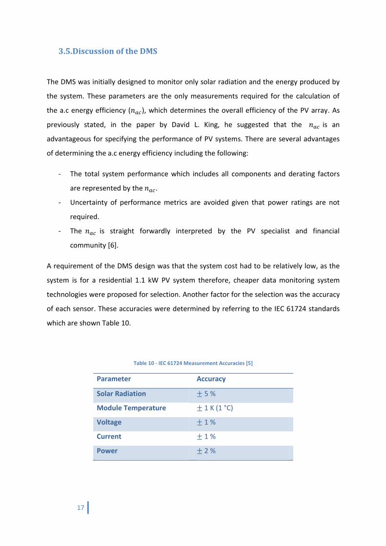
3.5. Discussion of the DMS

The DMS was initially designed to monitor only solar radiation and the energy produced by

the system. These parameters are the only measurements required for the calculation of

the a.c energy efficiency ( ), which determines the overall efficiency of the PV array. As

previously stated, in the paper by David L. King, he suggested that the is an

advantageous for specifying the performance of PV systems. There are several advantages

of determining the a.c energy efficiency including the following:

- The total system performance which includes all components and derating factors

are represented by the .

- Uncertainty of performance metrics are avoided given that power ratings are not

required.

- The is straight forwardly interpreted by the PV specialist and financial

community [6].

A requirement of the DMS design was that the system cost had to be relatively low, as the

system is for a residential 1.1 kW PV system therefore, cheaper data monitoring system

technologies were proposed for selection. Another factor for the selection was the accuracy

of each sensor. These accuracies were determined by referring to the IEC 61724 standards

which are shown Table 10.

Table 10 - IEC 61724 Measurement Accuracies [5]

Parameter Accuracy

Solar Radiation 5 %

Module Temperature 1 K (1 °C)

Voltage 1 %

Current 1 %

Power 2 %

18

The Onset HOBO data logger technology was selected to be used to design the DMS

because of the reasonable cost, the accuracy of all measurement components which were

all within close range of the IEC 61724 standard and the possibility to add more sensors if

desired. The SMA technology was similarly priced but the accuracy was of inferior quality

and the sensor capabilities were limited.

The chosen technology had the capabilities to add addition sensors, so more sensors were

added. Ultimately the HOBO data loggers were far superior in quality in term of accuracy

and cost. The total system cost for the DMS came to $2002.48 (including GST) which

includes solar radiation, energy (kWh), module temperature, a.c voltage and a.c current

sensors.

An investigation of where to mount the solar radiation sensor was also carried out. This was

done by using a solar pathfinder to determine the location on the array which was least

exposed to shading. Pictures of this investigation can be seen in Appendix B – Solar Pathfinder

Images.

19

4. Performance Analysis

A major task of this project is to analyse the performance of the MULPVS. As the MULPVS

has had a performance analysis carried out previously for the time period between August

2010 and May 2011 by Stephen Rose[3], there will be a continuation of this analysis for the

time period between June 2011 and August 2013.

4.1. Performance Analysis Method

The method for calculating the performance ratio and a.c energy efficiency follows the

method David L. King uses in his paper which was previously mentioned. This process

follows the IEC 61724 international standard. This method involves a number of

performance indices to complete a performance analysis. The main derived parameters are

as follows:

- Final Yield

- Reference Yield

- Performance Ratio

- System AC Energy Efficiency

Before the performance indices are calculated, the calculations of monthly yield were

obtained. Prior to this being done the sunny Webbox data files from the MULPVS have to be

converted to useable data. This process is outlined in Appendix C – Sunny SensorBox Data

Retrieval. Monthly ac energy produced are calculated by the following equation:

20

The monthly yield is calculated for each sub-array (inverter).Total system yields are obtained

by adding all the sub arrays outputs. The summary of these results can be found in Appendix

D – Performance Results. From this table an analysis was carried out exploring the best and

worst performing months, best and worst performing sub arrays, average output and total

system yield.

4.1.1. Final Yield

The final yield ( ) involves dividing the a.c energy produced ( ) by the system, by the

rated power output of the system ( ). is the measure of a.c energy (kWh) produced

by the PV system over time and is the array’s rated output (kWp) of the PV system

being measured.

4.1.2. Reference Yield

The reference yield ( ) involves dividing the cumulative plane of array irradiance ( ) by

thereference irradiance level ( ). is the measure of cumulative plane of array

irradiance (kWh/m2), and is the global reference irradiance level which is 1 kW/m2 as

suggested by IEC 61724[5].

4.1.3. Performance Ratio

The performance ratio ( ) involves dividing the final yield ( ) by the reference yield ( ).

The is the system’s and sub array’s overall conversion efficiency, of the energy received

21

to the energy exported to grid[3]. The accounts for the losses associated with the system

which include, temperature derating, dirt derating, cable losses, inverter efficiency, shading,

tolerances and degradation.

4.1.4. System AC Energy Efficiency

The system a.c energy efficiency ( ) involves cumulative plane of array irradiance ( ),

the array area (A) in m2 and the energy produced ( ) by the system. The in general

terms is the ratio of energy produced by the system to the energy supplied to system[6].

22

5. Performance Analysis Results of MULPVS

5.1. Solar Radiation

5.1.1. Method for Solar Radiation Data

The solar radiation data used for the performance analysis was initially obtained from the

Bureau of Meteorology (BoM) climate data [18]. The BoM has a Murdoch station (station

number 009187) which records the solar exposure for the latitude and longitude

coordinates of 32.08°S and 115.85°E respectively. The accuracy of this data is stated to be

7% for clear sky days and up to 20% for cloudy days[25].The BoM climate data website

produces the monthly mean daily solar radiation for each month from 1990 to present, for

solar exposure on a horizontal plane [26]. The PR results show abnormally high PR reaching

above 0.90, so it was assumed that there were some errors with these calculations and the

BoM solar radiation data was omitted.

Instead of using the BoM data, the solar radiation data produced by the Murdoch Met

Station, which is located at the latitude and longitude of 32.07 °S and 115.84 °E respectively,

was used. This data produced better results, as the radiation data showed higher readings

than that of the BoM. The low solar radiation data from the BoM and the high system yield

caused the performance ratio to be relatively high. The Met station had higher solar

radiation data measurements, which reduced the performance ratio values as there was

more available solar energy to be converted into power.

The horizontal data used was converted to plane of array data using an excel spreadsheet

which was provided by Dr Trevor Pryor of Murdoch University[27]. This spreadsheet was

produced by using the equations and theory from the text ‘Solar Engineering of Thermal

Processes’ by J.A. Duffie and W.A. Beckman[26]. Some of the equations to convert the

horizontal to in plane of array solar radiation used the sunset hour angle, extra-terrestrial

23

radiation, clearness index, beam radiation and diffuse radiation, the equations are then

applied using the KT method outline in the text.

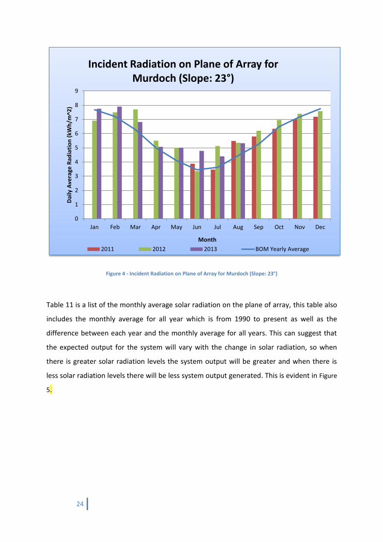
5.1.2. Solar Radiation Data Trend

The time period for the performance analysis of the MULPVS is from June 2011 to August

2013. Below, Figure 4is a graph showing the plane of array monthly mean daily solar

radiation for Murdoch for 2011, 2012 and 2013 during the analysis period. These results

were calculated from the Met Stations horizontal solar radiation measurements using the

method explained previously.

For the 2011 analysis period it can be seen that the months of July, October, November and

December produce results below average solar radiation levels, and June, August and

September produce results above average solar radiation levels. For 2012 it can be seen

that the months of January, June and December produce results below average solar

radiation levels and February, March, April, July, August, September, October and

November produce results above average solar radiation levels. For the 2013 analysis period

it can be seen that January to August all produce above average solar radiation levels.

24

Figure 4 - Incident Radiation on Plane of Array for Murdoch (Slope: 23°)

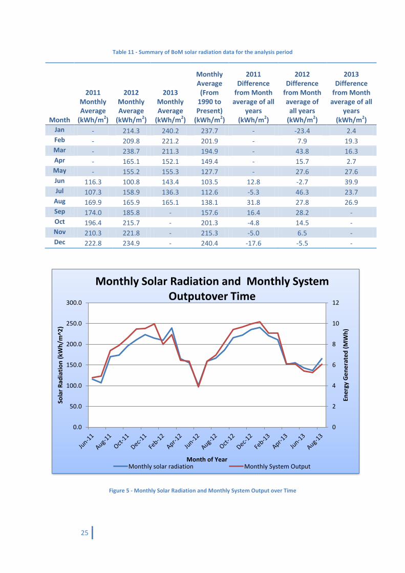
Table 11 is a list of the monthly average solar radiation on the plane of array, this table also

includes the monthly average for all year which is from 1990 to present as well as the

difference between each year and the monthly average for all years. This can suggest that

the expected output for the system will vary with the change in solar radiation, so when

there is greater solar radiation levels the system output will be greater and when there is

less solar radiation levels there will be less system output generated. This is evident in Figure

5.

0

1

2

3

4

5

6

7

8

9

Jan Feb Mar Apr May Jun Jul Aug Sep Oct Nov Dec

Dai

ly A

vera

ge R

adia

tio

n (

kWh

/m^2

)

Month

Incident Radiation on Plane of Array for Murdoch (Slope: 23°)

2011 2012 2013 BOM Yearly Average

25

Table 11 - Summary of BoM solar radiation data for the analysis period

Month

2011 Monthly Average

(kWh/m2)

2012 Monthly Average

(kWh/m2)

2013 Monthly Average

(kWh/m2)

Monthly Average

(From 1990 to Present)

(kWh/m2)

2011 Difference

from Month average of all

years (kWh/m2)

2012 Difference

from Month average of

all years (kWh/m2)

2013 Difference

from Month average of all

years (kWh/m2)

Jan - 214.3 240.2 237.7 - -23.4 2.4 Feb - 209.8 221.2 201.9 - 7.9 19.3 Mar - 238.7 211.3 194.9 - 43.8 16.3 Apr - 165.1 152.1 149.4 - 15.7 2.7 May - 155.2 155.3 127.7 - 27.6 27.6 Jun 116.3 100.8 143.4 103.5 12.8 -2.7 39.9 Jul 107.3 158.9 136.3 112.6 -5.3 46.3 23.7

Aug 169.9 165.9 165.1 138.1 31.8 27.8 26.9 Sep 174.0 185.8 - 157.6 16.4 28.2 - Oct 196.4 215.7 - 201.3 -4.8 14.5 - Nov 210.3 221.8 - 215.3 -5.0 6.5 - Dec 222.8 234.9 - 240.4 -17.6 -5.5 -

Figure 5 - Monthly Solar Radiation and Monthly System Output over Time

0

2

4

6

8

10

12

0.0

50.0

100.0

150.0

200.0

250.0

300.0

Ene

rgy

Ge

ne

rate

d (

MW

h)

Sola

r R

adia

tio

n (

kWh

/m^2

)

Month of Year

Monthly Solar Radiation and Monthly System Outputover Time

Monthly solar radiation Monthly System Output

26

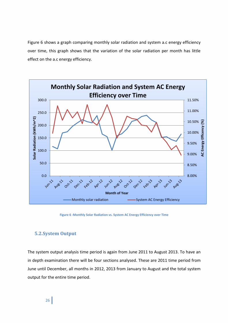
Figure 6 shows a graph comparing monthly solar radiation and system a.c energy efficiency

over time, this graph shows that the variation of the solar radiation per month has little

effect on the a.c energy efficiency.

Figure 6 -Monthly Solar Radiation vs. System AC Energy Efficiency over Time

5.2. System Output

The system output analysis time period is again from June 2011 to August 2013. To have an

in depth examination there will be four sections analysed. These are 2011 time period from

June until December, all months in 2012, 2013 from January to August and the total system

output for the entire time period.

8.00%

8.50%

9.00%

9.50%

10.00%

10.50%

11.00%

11.50%

0.0

50.0

100.0

150.0

200.0

250.0

300.0

AC

En

erg

y Ef

fice

ncy

(%

)

Sola

r R

adia

tio

n (

kWh

/m^2

)

Month of Year

Monthly Solar Radiation and System AC Energy Efficiency over Time

Monthly solar radiation System AC Energy Efficiency

27

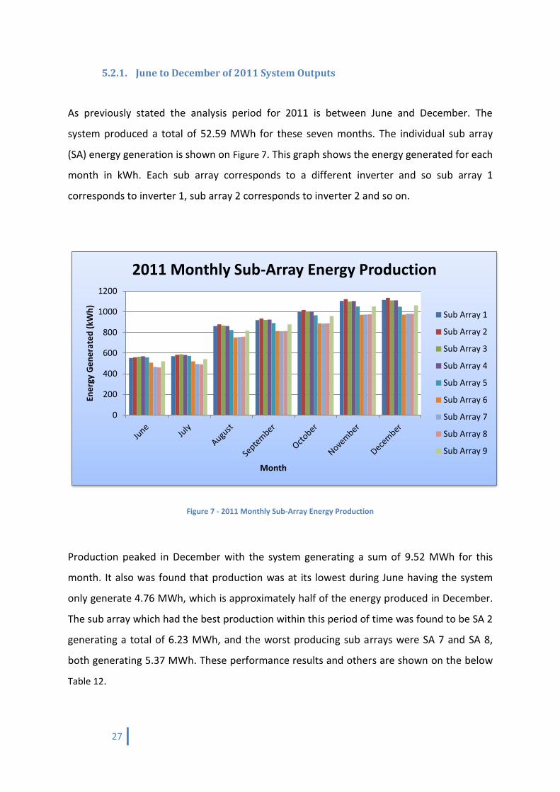
5.2.1. June to December of 2011 System Outputs

As previously stated the analysis period for 2011 is between June and December. The

system produced a total of 52.59 MWh for these seven months. The individual sub array

(SA) energy generation is shown on Figure 7. This graph shows the energy generated for each

month in kWh. Each sub array corresponds to a different inverter and so sub array 1

corresponds to inverter 1, sub array 2 corresponds to inverter 2 and so on.

Figure 7 - 2011 Monthly Sub-Array Energy Production

Production peaked in December with the system generating a sum of 9.52 MWh for this

month. It also was found that production was at its lowest during June having the system

only generate 4.76 MWh, which is approximately half of the energy produced in December.

The sub array which had the best production within this period of time was found to be SA 2

generating a total of 6.23 MWh, and the worst producing sub arrays were SA 7 and SA 8,

both generating 5.37 MWh. These performance results and others are shown on the below

Table 12.

0

200

400

600

800

1000

1200

Ene

rgy

Ge

ne

rate

d (

kWh

)

Month

2011 Monthly Sub-Array Energy Production

Sub Array 1

Sub Array 2

Sub Array 3

Sub Array 4

Sub Array 5

Sub Array 6

Sub Array 7

Sub Array 8

Sub Array 9

28

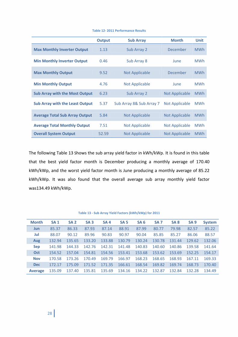
Table 12- 2011 Performance Results

Output Sub Array Month Unit

Max Monthly Inverter Output 1.13 Sub Array 2 December MWh

Min Monthly Inverter Output 0.46 Sub Array 8 June MWh

Max Monthly Output 9.52 Not Applicable December MWh

Min Monthly Output 4.76 Not Applicable June MWh

Sub Array with the Most Output 6.23 Sub Array 2 Not Applicable MWh

Sub Array with the Least Output 5.37 Sub Array 8& Sub Array 7 Not Applicable MWh

Average Total Sub Array Output 5.84 Not Applicable Not Applicable MWh

Average Total Monthly Output 7.51 Not Applicable Not Applicable MWh

Overall System Output 52.59 Not Applicable Not Applicable MWh

The following Table 13 Shows the sub array yield factor in kWh/kWp. It is found in this table

that the best yield factor month is December producing a monthly average of 170.40

kWh/kWp, and the worst yield factor month is June producing a monthly average of 85.22

kWh/kWp. It was also found that the overall average sub array monthly yield factor

was134.49 kWh/kWp.

Table 13 - Sub Array Yield Factors (kWh/kWp) for 2011

Month SA 1 SA 2 SA 3 SA 4 SA 5 SA 6 SA 7 SA 8 SA 9 System

Jun 85.37 86.33 87.93 87.14 88.91 87.99 80.77 79.98 82.57 85.22

Jul 88.07 90.12 89.96 90.83 90.97 90.04 85.85 85.27 86.06 88.57

Aug 132.94 135.65 133.20 133.88 130.79 130.24 130.78 131.44 129.62 132.06

Sep 141.98 144.33 142.76 142.31 141.48 140.83 140.60 140.86 139.58 141.64

Oct 154.52 157.04 154.81 154.56 153.41 153.68 153.62 153.69 152.25 154.17

Nov 170.58 173.26 170.49 169.79 166.97 168.23 168.65 168.93 167.11 169.33

Dec 172.17 175.09 171.52 171.35 166.61 168.54 169.82 169.74 168.73 170.40

Average 135.09 137.40 135.81 135.69 134.16 134.22 132.87 132.84 132.28 134.49

29

5.2.2. January to December 2012 System Outputs

The analysis period for 2012 is between January and December. The system output for 2012

was 92.75 MWh. During the months February, March, April, May and June the inverter of SA

3 was offline. This affected the system output for these months resulting in lower outputs.

Shown in Figure 8 is a graph of the monthly sub array power production for 2012 displaying

the variation of the energy generation over the year. It is interesting to note that if SA 3 was

online that the energy generated in March could have been similar to that of January if not

more.

Figure 8 - 2012 Monthly Sub – Array Energy Production

Production peaked in December with the system generating a sum of 9.98 MWh for this

month and it also was found that production was at its lowest during June having the

system only generate 3.43 MWh. The sub array which had the best production within the

period of time was found to be SA 2 generating a total of 11.46MWh and the worst

producing sub array was SA 3 generating 6.97 MWh. SA 3 produced a significantly lower

output for the previously stated reason, namely that this sub array was offline during the

months of February to June. These results and others are shown in Table 14 below.

0.00

200.00

400.00

600.00

800.00

1000.00

1200.00

1400.00

Ene

rgy

Ge

ne

rate

d (

kWh

)

Month

2012 Monthly Sub-Array Energy Production

Sub Array 1

Sub Array 2

Sub Array 3

Sub Array 4

Sub Array 5

Sub Array 6

Sub Array 7

Sub Array 8

Sub Array 9

30

Table 14 - 2012 Performance Results

Output Sub Array Month Unit

Max Monthly Inverter Output 1.20 Sub Array 2 January MWh

Min Monthly Inverter Output 0.37 Sub Array 8 June MWh

Max Monthly Output 9.98 Not Applicable December MWh

Min Monthly Output 3.43 Not Applicable June MWh

Sub Array with the Most Output 11.46 Sub Array 2 Not Applicable MWh

Sub Array with the Least Output 6.97 Sub Array 3 Not Applicable MWh

Average Total Sub Array Output 10.31 Not Applicable Not Applicable MWh

Average Total Monthly Output 7.73 Not Applicable Not Applicable MWh

Overall System Output 92.75 Not Applicable Not Applicable MWh

The following Table 15 shows the sub array yield factor in kWh/kWp. It is evident in this

table that the high yield factor months are January and December producing a monthly

average of 178.11 kWh/kWp and 178.68 kWh/kWp, respectively. The lowest yield factor

month is significantly lower with June producing a monthly average of 61.70 kWh/kWp. It

was found that the overall average sub array monthly yield factor was138.61 kWh/kWp.

Table 15 - Sub Array Yield Factors (kWh/kWp) for 2012

Month SA 1 SA 2 SA 3 SA 4 SA 5 SA 6 SA 7 SA 8 SA 9 Average

Jan 182.55 185.61 158.08 182.01 176.74 178.78 180.14 180.11 178.96 178.11

Feb 163.08 165.65 0.00 162.90 160.29 160.87 161.46 161.54 159.94 143.97

Mar 182.34 185.38 0.00 182.78 180.10 179.57 180.05 180.19 178.72 161.01

Apr 127.43 129.72 0.00 128.05 125.68 124.70 125.91 126.11 124.78 112.48

May 113.86 117.08 0.00 117.71 114.88 114.17 109.52 110.22 109.54 100.78

Jun 70.68 71.21 0.00 70.75 74.27 73.14 64.39 64.01 66.82 61.70

Jul 117.60 114.26 117.50 116.28 117.12 116.10 107.38 108.10 109.45 113.75

Aug 126.66 124.64 125.60 127.29 123.44 122.43 122.22 122.45 121.14 123.99

Sep 149.57 146.94 147.24 149.29 146.79 145.96 146.06 146.11 144.67 146.96

Oct 171.36 168.96 169.03 171.69 167.80 167.66 167.95 167.95 166.24 168.74

Nov 173.97 176.43 175.73 173.09 171.01 172.06 172.78 172.90 170.46 173.16

Dec 180.49 183.16 182.03 179.30 174.82 176.41 177.81 177.79 176.34 178.68

Average 146.63 147.42 89.60 146.76 144.41 144.32 142.97 143.12 142.25 138.61

31

5.2.3. January to August 2013 System Outputs

The analysis period for this section is from January to August of 2013. The system produced

a total of 57.33 MWh for these seven months. The monthly sub array power production is

shown in Figure 9.

Figure 9 - 2013 Monthly Sub Array Energy Production

Production has so far peaked in January with the system generating a sum of 10.17 MWh

and it also was found that production was at its lowest during July generating a sum of 3.91

MWh. The sub array which had the best production within the period of time was found

tobe SA 3 generating a total of 6.84 MWh and the worst producing sub array was SA 8

generating 5.75 MWh. These results and others are shown in Table 16 below.

0.00

200.00

400.00

600.00

800.00

1000.00

1200.00

1400.00

January February March April May June July August

Ene

rgy

Ge

ne

rate

d (

kWh

)

Month

2013 Monthly Sub-Array Power Production

Sub Array 1

Sub Array 2

Sub Array 3

Sub Array 4

Sub Array 5

Sub Array 6

Sub Array 7

Sub Array 8

32

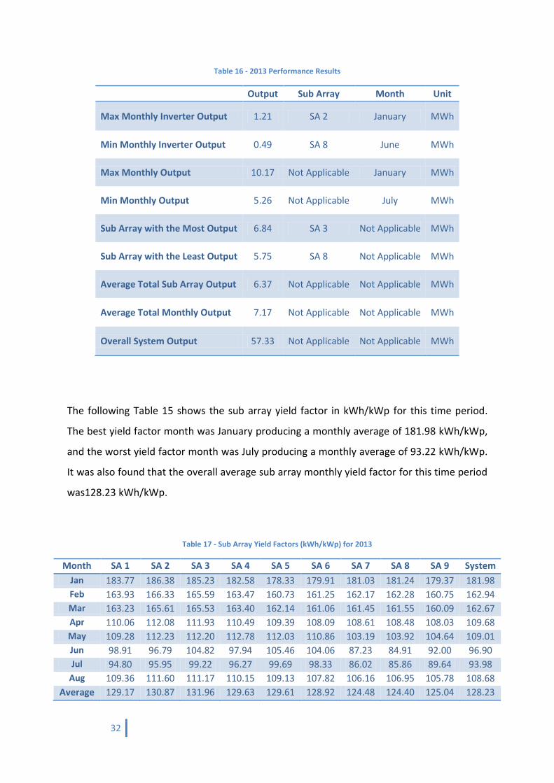
Table 16 - 2013 Performance Results

Output Sub Array Month Unit

Max Monthly Inverter Output 1.21 SA 2 January MWh

Min Monthly Inverter Output 0.49 SA 8 June MWh

Max Monthly Output 10.17 Not Applicable January MWh

Min Monthly Output 5.26 Not Applicable July MWh

Sub Array with the Most Output 6.84 SA 3 Not Applicable MWh

Sub Array with the Least Output 5.75 SA 8 Not Applicable MWh

Average Total Sub Array Output 6.37 Not Applicable Not Applicable MWh

Average Total Monthly Output 7.17 Not Applicable Not Applicable MWh

Overall System Output 57.33 Not Applicable Not Applicable MWh

The following Table 15 shows the sub array yield factor in kWh/kWp for this time period.

The best yield factor month was January producing a monthly average of 181.98 kWh/kWp,

and the worst yield factor month was July producing a monthly average of 93.22 kWh/kWp.

It was also found that the overall average sub array monthly yield factor for this time period

was128.23 kWh/kWp.

Table 17 - Sub Array Yield Factors (kWh/kWp) for 2013

Month SA 1 SA 2 SA 3 SA 4 SA 5 SA 6 SA 7 SA 8 SA 9 System

Jan 183.77 186.38 185.23 182.58 178.33 179.91 181.03 181.24 179.37 181.98

Feb 163.93 166.33 165.59 163.47 160.73 161.25 162.17 162.28 160.75 162.94

Mar 163.23 165.61 165.53 163.40 162.14 161.06 161.45 161.55 160.09 162.67

Apr 110.06 112.08 111.93 110.49 109.39 108.09 108.61 108.48 108.03 109.68

May 109.28 112.23 112.20 112.78 112.03 110.86 103.19 103.92 104.64 109.01

Jun 98.91 96.79 104.82 97.94 105.46 104.06 87.23 84.91 92.00 96.90

Jul 94.80 95.95 99.22 96.27 99.69 98.33 86.02 85.86 89.64 93.98

Aug 109.36 111.60 111.17 110.15 109.13 107.82 106.16 106.95 105.78 108.68

Average 129.17 130.87 131.96 129.63 129.61 128.92 124.48 124.40 125.04 128.23

33

5.2.4. Overall System Output

The time period for this performance analysis is from June 2011 to August 2013. The overall

system output for this 27 month time period is 202.67 MWh. Shown in Figure 10 is a graph of

the monthly system output for the analysis period. This shows the variation of the energy

generated from month to month.

Figure 10 - Overall System Output

The production of energy for the overall time period peaked during January 2013 with the

system generating a sum of 10.17 MWh in terms of monthly output. The system saw its

lowest production in June 2012 generating a low3.43MWh. It was found that the sub array

which had the best production was SA 2 generating a total of 24.48MWh which is 12.08 % of

total production and the worst producing sub array was SA 3 generating a total of 19.97

MWh which is 9.85 % of total production. These results and others are shown on the below

Table 18.

0

2

4

6

8

10

12

Jan Feb Mar Apr May Jun Jul Aug Sep Oct Nov Dec

Ene

rgy

Ge

ne

rate

d (

MW

h)

Month

System Monthly Output

2011

2012

2013

34

Table 18 - Performance Results of the Overall System

Output Sub Array Month Unit

Max Monthly Inverter Output 1.21 Sub Array 2 January 2013 MWh

Min Monthly Inverter Output 0.37 Sub Array 8 June 2012 MWh

Max Monthly Output 10.17 Not Applicable January 2013 MWh

Min Monthly Output 3.43 Not Applicable June 2012 MWh

Sub Array with the Most Output 24.48 Sub Array 2 Not Applicable MWh

Sub Array with the Least Output 19.97 Sub Array 3 Not Applicable MWh

Average Total Sub Array Output 22.52 Not Applicable Not Applicable MWh

Average Total Monthly Output 7.51 Not Applicable Not Applicable MWh

Overall System Output 202.67 Not Applicable Not Applicable MWh

The following Figure 11 shows the graph of the monthly average yield factor in kWh/kWp

over the 27 month period. It can be seen in this graph that the best yield factor month was

January in 2013 producing a monthly average of 181.98 kWh/kWp, and the worst yield

factor month was June in 2012 producing a monthly average of 61.70 kWh/kWp. It was also

found that the overall average sub array monthly average yield factor for this 27 month

period to be 134.47 kWh/kWp. In Appendix D – Performance Results a table of monthly sub

array and total system yield factor can be seen.

35

Figure 11 - Monthly Average Yield Factor per Year (kWh/kWp)

0

2

4

6

8

10

12

Jan Feb Mar Apr May Jun Jul Aug Sep Oct Nov Dec

Ene

rgy

Ge

ne

rate

d (

MW

h)

Month

Monthly Average Yield Factor per Year

2011

2012

2013

36

5.2.5. System Output Discussion

Factors that can affect the system output are shading, dirt build up, temperature and solar

radiation levels. The factors of dirt build up and temperatures are assumptions as

investigation of these aspects were not carried out. It can be assumed that the build up of

dirt has affected the PV system during the months of 2013. During the months of April, May,

July and August there were greater levels of solar radiation but the system outputs for these

months were lower than in the same month of 2012, this can also be caused by shading

from the trees which have grown from year to year. It was found that the average daily

temperature during January for 2012 and 2013 was 33.5 °C and 31.7 °C respectively, while

the system outputs were 9.94 MWh and 10.17 MWh respectively. This suggests that high

temperatures can affect the power output of the panels. When looking at the variation of

solar radiation this directly affects the power output of the PV system.

The best sub array in terms of energy generation was found to be SA 2. It can be assumed

that this was due to the location of the array as it is nearly in the middle of the system being

exposed to shading the least. The peak output of the array is 6.48 kW. It was found that the

worst sub array was SA 3.This is because during the months from February to June of 2012

the array was offline. It can be assumed that if SA 3 was online during the whole 27 month

period the worst array would then be SA 7 as it is affected by shading and the array has a

peak output of 5.775 kW.

The best producing month of the system was found to be January 2013.This is a result of

high levels of solar radiation and the lower temperatures present. The worst producing

month was June of 2012 and this is a result of low solar radiation levels, shading on the

system as well as the SA 3 being offline during this month.

37

5.3. Performance Ratio

As previously stated the performance ratio ( ) involves dividing the final yield ( ) by the

reference yield ( ).

5.3.1. System Performance

The following Figure 12 is a graph of the monthly system performance ratio for the analysis

period. A slight trend that can be seen in the graph is that the is low during the winter

months, which could be the affect of greater shading on the array during these months.

Figure 12- Monthly System Performance Ratio

The below Table 19-System Performance Ratio Table 19 shows a list of the monthly

performance ratios for each year and a percentage difference between years 2011 and

2012, and 2012 and 2013. It can be seen that the highest was during January 2012 with a

value of 0.83 and the lowest was during June 2012 with a value of 0.61. The

percentage difference between 2012 and 2013 was negative for the months from February

0.60

0.65

0.70

0.75

0.80

0.85

Jan Feb Mar Apr May Jun Jul Aug Sep Oct Nov Dec

Pe

rfo

rman

ce R

atio

Month

Monthly System Performance Ratio

2011

2012

2013

38

to June, this is caused by SA 3 being offline. The percentage difference for the months

from August to December between the years of 2011 and 2012 are fairly close, this indicate

that the for 2011 and 2012 for the month of August to December were similar.

Table 19-System Performance Ratio

Month 2011

2012

2013

Percentage Difference

2011 and 2012

Percentage Difference

2012 and 2013

January - 0.83 0.76 - 7.27%

February - 0.68 0.74 - -5.41%

March - 0.67 0.77 - -9.93%

April - 0.68 0.72 - -4.37%

May - 0.65 0.70 - -5.66%

June 0.73 0.61 0.68 12.44% -6.79%

July 0.83 0.72 0.69 10.94% 2.64%

August 0.78 0.75 0.66 2.98% 8.90%

September 0.81 0.79 - 2.31% -

October 0.79 0.78 - 0.27% -

November 0.81 0.78 - 2.46% -

December 0.77 0.76 - 0.40% -

5.3.2. Sub Array Performance

The Figure 13 is a graph showing the monthly sub array performance ratios. It can be seen

that there is a seasonal trend that the winter months produce a lower value for the sub

arrays. It is also noticeable that at times the SA 7, SA 8 and SA 9 produce lower values

than the other sub arrays for each month during the analysis period. It was found that the

sub array producing the highest monthly average to be SA 4 with a value of 0.734 and the

lowest monthly average to be SA 3 with a value of 0.600. The maximum occurred in

January 2012 and was 0.832. The system had a low occurring in June 2013 with a value of

0.569. The reason behind the fluctuation in the will be mentioned in the performance

ratio discussion. A table of all monthly sub array performance ratios can be seen in Appendix

D – Performance Results.

39

Figure 13 - Monthly Sub Array Performance Ratio

0.50

0.55

0.60

0.65

0.70

0.75

0.80

0.85

Jun

e

July

Au

gust

Sep

tem

be

r

Oct

ob

er

No

vem

be

r

De

cem

ber

Jan

uar

y

Feb

ruar

y

Mar

ch

Ap

ril

May

Jun

e

July

Au

gust

Sep

tem

be

r

Oct

ob

er

No

vem

be

r

De

cem

ber

Jan

uar

y

Feb

ruar

y

Mar

ch

Ap

ril

May

Jun

e

July

Au

gust

2011 2011 2011 2011 2011 2011 2011 2012 2012 2012 2012 2012 2012 2012 2012 2012 2012 2012 2012 2013 2013 2013 2013 2013 2013 2013 2013

Pe

rfo

rman

ce R

atio

Month

2012 Sub Array Performance Ratio

Sub Array 1 Sub Array 2 Sub Array 3 Sub Array 4 Sub Array 5 Sub Array 6 Sub Array 7 Sub Array 8 Sub Array 9

40

5.3.3. Performance Ratio Discussion

Similar to the factors that affect the system yield, shading, dirt build up, and solar radiation

levels also affect . It can be seen in Figure 13 the graph of monthly sub array performance

ratios, there seems to be a trend that the monthly values in 2013 have decreased when

compared to the previous year’s results. This decrease could be caused by dirt build up on

the panels, this inhibits the ability for the available solar radiation to be converted in power.

Another reason for this is the possibility of increased shading on the PV array, as trees grow

over time.

Fluctuation in the can be caused by the inaccuracies in the solar radiation

measurements, this is because the cumulative plane of array irradiance measurement is

used in the equations to determine the . If the pyranometer measurements were

recorded to be greater or less than the actual level of irradiance this will cause the

calculation to be less or more respectively, than the expected . The calculation used,

involved irradiance measurements which were recorded from a different site to that of the

PV array, this may have caused some discrepancies in the results.

5.5. Shading

The PV array located on the roof of Murdoch University Library is situated near numerous

large trees that cause shading. During the summer months shading minimally affects the PV

array and this is evident the results in Figure 14. SA 4 is only slightly affected by shading. The

day represented in this graph is a sunny day in January.

Shading mainly affects the months during winter, this is evident in Figure 15 to Figure 17.

The day represented in these graphs is a day with no cloud cover to inhibit the solar

radiation levels throughout the day.

41

Figure 14 - Shading Effects on Sub Arrays (January)

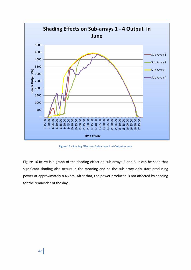
Figure 15 below is the graph of shading effects for sub arrays 1 to 4 for a sunny day in June.

It can be seen that shading is mostly present during the morning hours for the four sub

arrays.

0

1000

2000

3000

4000

5000

60005

:15

:00

5:5

0:0

0

6:2

5:0

0

7:0

0:0

0

7:3

5:0

0

8:1

0:0

0

8:4

5:0

0

9:2

0:0

0

9:5

5:0

0

10

:30

:00

11

:05

:00

11

:40

:00

12

:15

:00

12

:50

:00

13

:25

:00

14

:00

:00

14

:35

:00

15

:10

:00

15

:45

:00

16

:20

:00

16

:55

:00

17

:30

:00

18

:05

:00

18

:40

:00

19

:15

:00

Po

we

r O

utp

ut

(W)

Time of Day

Shading Effects on Sub Arrays (January) Sub Array 1

Sub Array 2

Sub Array 3

Sub Array 4

Sub Array 5

Sub Array 6

Sub Array 7

Sub Array 8

Sub Array 9

42

Figure 15 - Shading Effects on Sub-arrays 1 - 4 Output in June

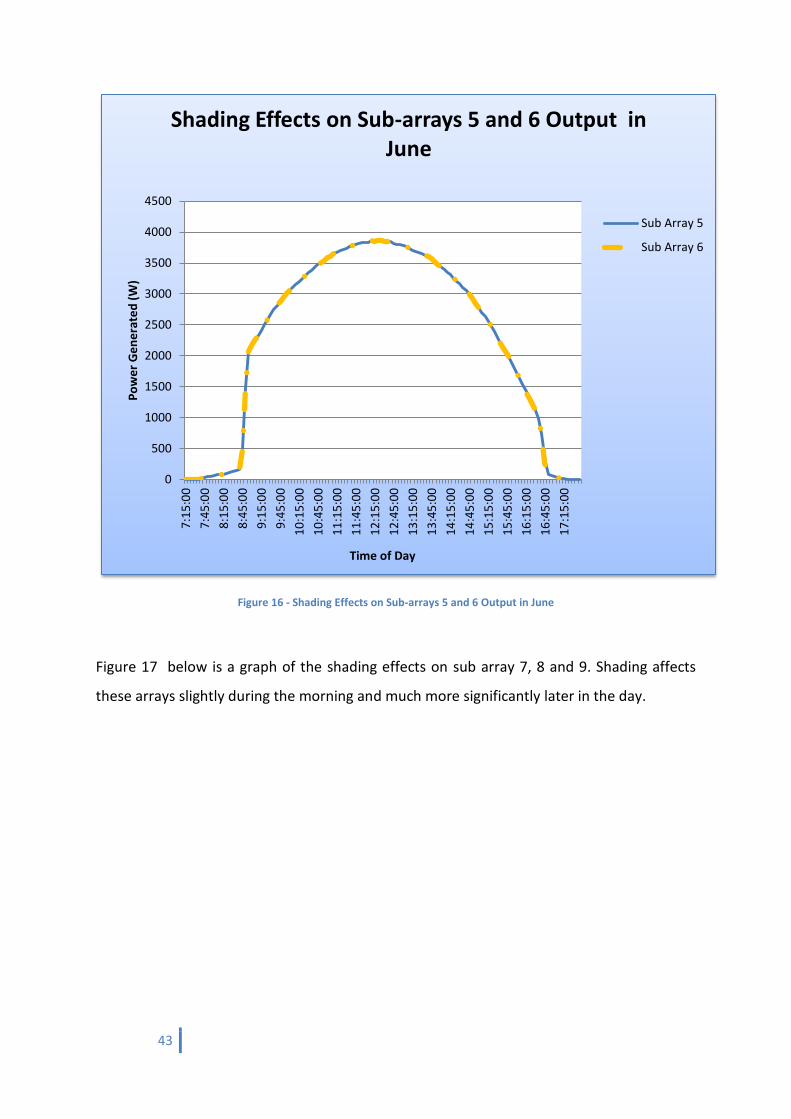
Figure 16 below is a graph of the shading effect on sub arrays 5 and 6. It can be seen that

significant shading also occurs in the morning and so the sub array only start producing

power at approximately 8.45 am. After that, the power produced is not affected by shading

for the remainder of the day.

0

500

1000

1500

2000

2500

3000

3500

4000

4500

50007

:15

:00

7:4

0:0

08

:05

:00

8:3

0:0

08

:55

:00

9:2

0:0

09

:45

:00

10

:10

:00

10

:35

:00

11

:00

:00

11

:25

:00

11

:50

:00

12

:15

:00

12

:40

:00

13

:05

:00

13

:30

:00

13

:55

:00

14

:20

:00

14

:45

:00

15

:10

:00

15

:35

:00

16

:00

:00

16

:25

:00

16

:50

:00

17

:15

:00

Po

we

r O

utp

ut

(W)

Time of Day

Shading Effects on Sub-arrays 1 - 4 Output in June

Sub Array 1

Sub Array 2

Sub Array 3

Sub Array 4

43

Figure 16 - Shading Effects on Sub-arrays 5 and 6 Output in June

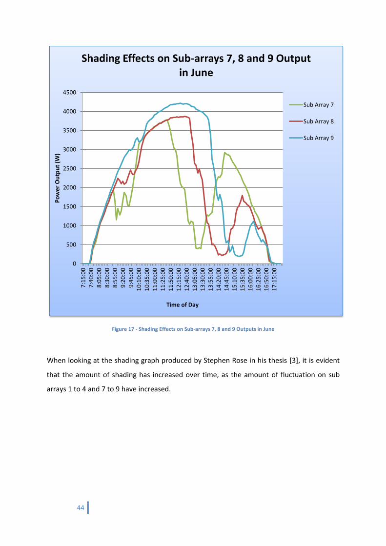
Figure 17 below is a graph of the shading effects on sub array 7, 8 and 9. Shading affects

these arrays slightly during the morning and much more significantly later in the day.

0

500

1000

1500

2000

2500

3000

3500

4000

4500

7:1

5:0

0

7:4

5:0

0

8:1

5:0

0

8:4

5:0

0

9:1

5:0

0

9:4

5:0

0

10

:15

:00

10

:45

:00

11

:15

:00

11

:45

:00

12

:15

:00

12

:45

:00

13

:15

:00

13

:45

:00

14

:15

:00

14

:45

:00

15

:15

:00

15

:45

:00

16

:15

:00

16

:45

:00

17

:15

:00

Po

we

r G

en

era

ted

(W

)

Time of Day

Shading Effects on Sub-arrays 5 and 6 Output in June

Sub Array 5

Sub Array 6

44

Figure 17 - Shading Effects on Sub-arrays 7, 8 and 9 Outputs in June

When looking at the shading graph produced by Stephen Rose in his thesis [3], it is evident

that the amount of shading has increased over time, as the amount of fluctuation on sub

arrays 1 to 4 and 7 to 9 have increased.

0

500

1000

1500

2000

2500

3000

3500

4000

4500

7:1

5:0

07

:40

:00

8:0

5:0

08

:30

:00

8:5

5:0

09

:20

:00

9:4

5:0

01

0:1

0:0

01

0:3

5:0

01

1:0

0:0

01

1:2

5:0

01

1:5

0:0

01

2:1

5:0

01

2:4

0:0

01

3:0

5:0

01

3:3

0:0

01

3:5

5:0

01

4:2

0:0

01

4:4

5:0

01

5:1

0:0

01

5:3

5:0

01

6:0

0:0

01

6:2

5:0

01

6:5

0:0

01

7:1

5:0

0

Po

we

r O

utp

ut

(W)

Time of Day

Shading Effects on Sub-arrays 7, 8 and 9 Output in June

Sub Array 7

Sub Array 8

Sub Array 9

45

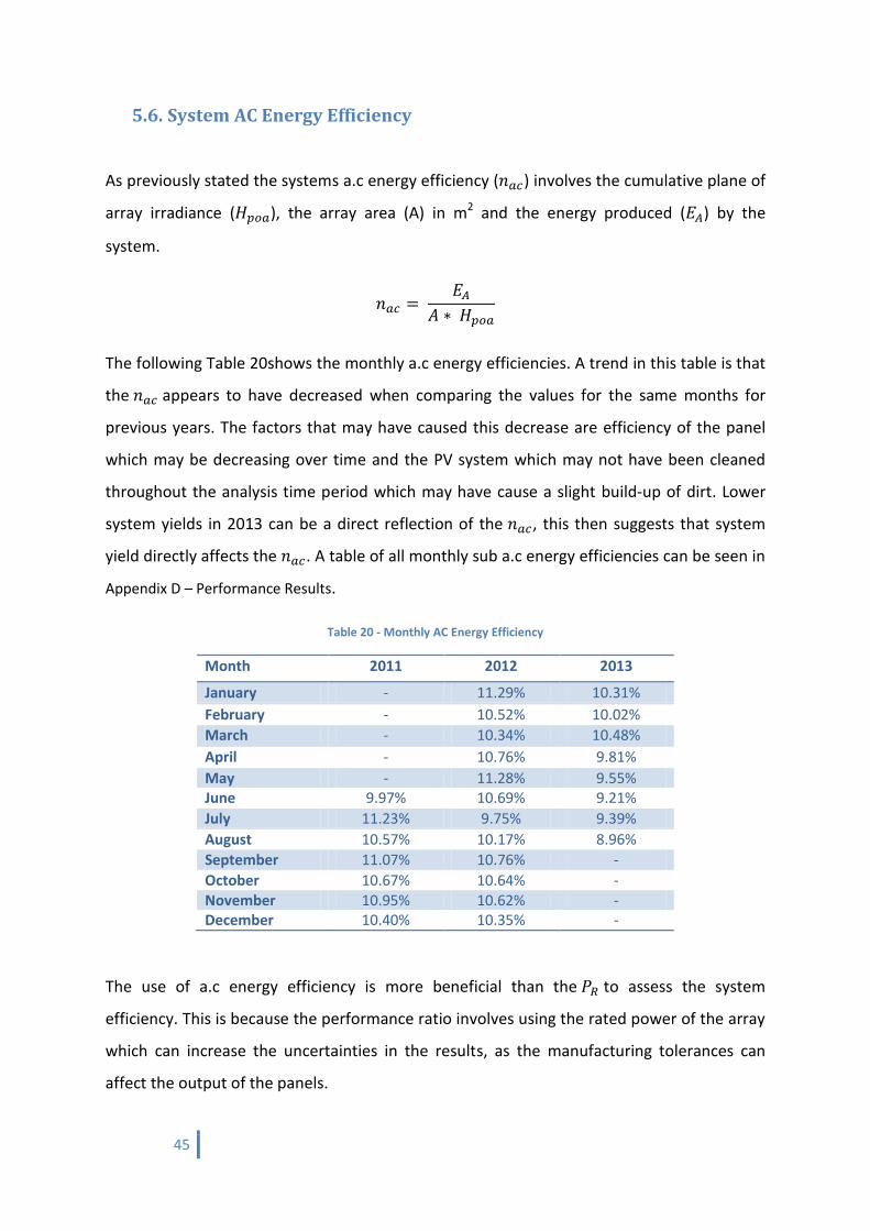
5.6. System AC Energy Efficiency

As previously stated the systems a.c energy efficiency ( ) involves the cumulative plane of

array irradiance ( ), the array area (A) in m2 and the energy produced ( ) by the

system.

The following Table 20shows the monthly a.c energy efficiencies. A trend in this table is that

the appears to have decreased when comparing the values for the same months for

previous years. The factors that may have caused this decrease are efficiency of the panel

which may be decreasing over time and the PV system which may not have been cleaned

throughout the analysis time period which may have cause a slight build-up of dirt. Lower

system yields in 2013 can be a direct reflection of the , this then suggests that system

yield directly affects the . A table of all monthly sub a.c energy efficiencies can be seen in

Appendix D – Performance Results.

Table 20 - Monthly AC Energy Efficiency

Month 2011 2012 2013

January - 11.29% 10.31%

February - 10.52% 10.02%

March - 10.34% 10.48%

April - 10.76% 9.81%

May - 11.28% 9.55% June 9.97% 10.69% 9.21%

July 11.23% 9.75% 9.39%

August 10.57% 10.17% 8.96%

September 11.07% 10.76% -

October 10.67% 10.64% - November 10.95% 10.62% - December 10.40% 10.35% -

The use of a.c energy efficiency is more beneficial than the to assess the system

efficiency. This is because the performance ratio involves using the rated power of the array

which can increase the uncertainties in the results, as the manufacturing tolerances can

affect the output of the panels.

46

5.7. Comparing PV Technologies

Performance ratio, AC energy efficiency and monthly average yield factor in kWh/kWp, are

the parameters which will be looked at when comparing the two PV technologies used in

the MULPVS, these two technologies are Kyocera 135 W multi- crystalline (Poly –Si) module

and the Sun grid 175 W mono- crystalline (Mono- Si) module. The following Table 21

displays the PV cell results of the monthly average sub array Performance ratio, ac energy

efficiency and the yield factor. It can be seen that the poly – Si module produces the best

result for all three parameters, indicating that it is the best performing module achieving a

closer rated output than the mono- Si module. The PV cell averages can be seen in the tables

in Appendix D – Performance Results.

Table 21 - PV Cell Results

Poly- Si Mono- Si System

Monthly Average Sub Array Performance Ratio

0.734 0.716 0.724

Monthly Average Sub Array AC Energy Efficiency

10.29% 10.22% 10.25%

Monthly Average Sub Array Yield Factor (kWh/kWp)

139.28 135.77 137.29

47

6. Future Works

Through this analysis it was found that the Sunny Sensorbox went offline during 2012 so

possible solutions should be looked at to solve this problem. When this issue has been

resolved, the analysis of module temperature, ambient temperature, and wind speed

should be applied in the performance analysis. A performance analysis using the solar

radiation measurements from the Sunny Sensorbox should be completed for more accurate

results. In saying this, it would be very useful if the continuation of the performance analysis

of the MULPVS is undertaken to assess the system as it ages.

Maintenance of the MULPVS should be look at, and the effects of shading and the dirt

derating factors should be analysed in depth.

The installation of the LPVS data monitoring system should be completed so a performance

analysis of this residential system can be carried out, to assess the performance of

residential PV System. Then a comparison between the performance of this system and the

MULPVS can be completed.

Another possible task is once the PV Training Facility data monitoring system is running on

the Energy and Engineering building at Murdoch University, performance analysis’ of this

system could be carried out and a comparison of all PV systems mentioned can be

compared.

48

7. Conclusion

The design of developing a data monitoring system entailed researching feasible and

accurate technologies. The requirements of this task were determined by reviewing

limitations and assessing the desired out comes. The selection process involved referring to

relevant standards. After comparison and consideration the HOBO Data Logger technology

was found to be most suitable for this project at it was cost effective and proved to have

acceptable accuracies. The purchased system comprised of five sensors; solar radiation, ac

output energy, module temperature, a.c voltage and a.c current sensors. This system has

the capabilities to add more sensors if desired.

The performance analysis of the Murdoch University Library Photovoltaic System was

completed over a 27 month period. A data retrieval process was produced as this was

completed in order to attain useful data for the performance analysis. It was uncovered that

sub array 3 was offline from February 2012 until June 2012. The analysis considered system

yield, performance ratio and a.c energy efficiency. Assumption were made as to what

factors could influence these parameters. It was found that the Kyocera poly- crystalline

modules performed slightly better in comparison to the Sun Grid mono- crystalline modules.

Problems with the Sunny SensorBox was found and recommendations for possible solution

have been suggested for future work.

49

8. References

1. Clean Energy Australia Report 2012. 2013 [cited 2013 15/8/13

]; Available from:

http://www.cleanenergycouncil.org.au/resourcecentre/reports/cleanenergyaustralia.h

tml.

2. Engineering and Information Technology. 2013 [cited 2013 15/8/13]; Available from:

http://www.murdoch.edu.au/School-of-Engineering-and-Information-

Technology/Facilities/.

3. Rose, S., Performance evaluation, simulation and design assessment of the 56kWp

Murdoch University Library photovoltaic system. 2011, Murdoch University.

4. Riou, M., Monitoring and data acquisition system for the photovoltaic training facility on

the engineering and energy building. 2012, Murdoch University.

5. IEC, IEC 61724: Photovoltaic system performance monitoring – Guidelines for

measurement, data exchange and analysis. 1998, International Electrotechnical

Commission: Geneva.

6. King, D.L. More efficient methods for specifying and monitoring PV system performance. in

2011 37th IEEE Photovoltaic Specialists Conference (PVSC 2011), 19-24 June 2011. 2011.

Piscataway, NJ, USA: IEEE.

7. Murdoch_University, 2009 Annual Report - A Year of Achievements. 2009: Western

Australia.

8. Kyocera, KD135GH-2P (Brochure). Kyocera Corperation.

9. Sungrid, Photovoltaic module type: SG-175M5 (brochure). Sungrid Ltd: Fremantle.

10. SMA, SMC 4000A 500A 6000A Technical Data Sheet. SMA Solar Technology AG: Niestetal.

11. SunRise, SR Module SR-M572200-1 SR-M572195-1 SR-M572190 SR-M572185 SR-

M572180 SR-M572175. SUNRISE SOLARTECH CO LTD.

12. SMA, Sunny Boy 1100/ 1700. SMA Solar Technology AG: Niestetal.

13. Corporation, O.C. Silicon Pyranometer Smart Sensor (Part # S-LIB-M003) 2010; Available

from: http://www.onsetcomp.com/files/manual_pdfs/6708-D-MAN-S-LIB.pdf.

14. SMA. SUNNY PORTAL. 2013; Available from: http://www.sma-

australia.com.au/en_AU/products/monitoring-systems/sunny-portal.html.

15. SMA. SUNNY EXPLORER. 2013; Available from: http://www.sma-

australia.com.au/en_AU/products/software/sunny-explorer.html.

16. SMA. Accessories. 2013; Available from: http://www.sma-

australia.com.au/en_AU/products/accessories.html.

50

17. Corporation, O.C. 12-Bit Temperature Smart Sensor (Part # S-TMB-M0XX) 2008 [cited

2013; Available from: http://www.onsetcomp.com/files/manual_pdfs/7105-G-MAN-S-

TMB.pdf.

18. Meteorology, B.o. Climate Data Online. 2013 [cited 2013; Available from:

http://www.bom.gov.au/climate/data/index.shtml.

19. Temp, O. WattNode Advanced Pulse - kilowatt hour kWh energy meter. 2013 [cited 2013;

Available from: http://www.onetemp.com.au/p/1176/wattnode-advanced-pulse-

kilowatt-hour-kwh-energy-meter.

20. Temp, O. 300 Volt AC Potential Transformer - T-MAG-SPT-300. 2013 [cited 2013;

Available from: http://www.onetemp.com.au/p/1170/300-volt-ac-potential-

transformer-t-mag-spt-300.

21. Jessie Copper, A.B., Ted Spooner, Martina Calais, Trevor Pryor, Muriel Watt, Draft -

Technical Guidelines for Monitoring and Analysing Photovoltaic Systems. 2013.

22. Temp, O. FlexSmart TRMS Module (2 channels) - S-FS-TRMSA for H22 2013 [cited 2013;

Available from: http://www.onetemp.com.au/p/1169/flexsmart-trms-module-2-

channels-s-fs-trmsa-for-h22.

23. Temp, O. Mini Split-core AC Current Transformers - T-MAG-0400 - for U30 and H22

Loggers. 2013 [cited 2013; Available from: http://www.onetemp.com.au/p/1522/mini-

split-core-ac-current-transformers-t-mag-0400-for-u30-and-h22-loggers.

24. Temp, O. HOBO Energy Logger - H22-001 - Multi Channel. 2013 [cited 2013; Available

from: http://www.onetemp.com.au/p/932/hobo-energy-logger-h22-001-multi-

channel.

25. Meteorology, B.o. Monthly mean daily global solar exposure - Murdoch. 2013 [cited 2013;

Available from:

http://www.bom.gov.au/jsp/ncc/cdio/weatherData/av?p_nccObsCode=203&p_display_

type=dataFile&p_startYear=&p_c=&p_stn_num=009187.

26. John Duffie, W.B., Solar Engineering of Thermal Processes. 3rd Edition ed. 2006, New

Jersey: John Wiley and Sons, Inc.

27. Pryor, T., Solar04. Unknown: Murdoch University: Perth.

51

9. Appendix

All the appendices can be found on the attached CD Rom.

Appendix A– Design Specification

Appendix B – Solar Pathfinder Images

Appendix C – Sunny SensorBox Data Retrieval

Appendix D – Performance Results