Embed Size (px)
Citation preview
ABSTRACT
Title of Document: DESIGN OF A NOVEL PORTABLE FLOW
METER FOR MEASUREMENT OF
AVERAGE AND PEAK INSPIRATORY
FLOW
Shaya Jamshidi, M.S., 2009
Directed By: Professor Dr. Arthur T. Johnson, Fischell
Department of Bioengineering
The maximum tolerable physical effort that workers can sustain is of
significance across many industrial sectors. These limits can be determined by
assessing physiological responses to maximal workloads. Respiratory response is the
primary metric to determine energy expenditure in industries that use respirator
masks to protect against airborne contaminants. Current studies fail to evaluate
endurance under conditions that emulate employee operating environments. Values
obtained in artificial laboratory settings may be poor indicators of respiratory
performance in actual work environments. To eliminate such discrepancies,
equipment that accurately measures peak respiratory flows in situ is needed. This
study provides a solution in the form of a novel portable flow meter design that
accurately measures average and peak inspiratory flow of a user wearing an M40A1
respirator mask.

DESIGN OF A NOVEL PORTABLE FLOW METER FOR MEASUREMENT OF
AVERAGE AND PEAK INSPIRATORY FLOW
By
Shaya Jamshidi
Thesis submitted to the Faculty of the Graduate School of the
University of Maryland, College Park, in partial fulfillment
of the requirements for the degree of
Masters of Science
2009
Advisory Committee:
Professor Dr. Arthur Johnson, Chair
Dr. Adel Shirmohammadi
Dr. Fredrick Wheaton

© Copyright by
Shaya Jamshidi
2009

ii
Acknowledgments No graduate student can write a thesis by themselves, and this graduate student is no
exception. I would like to thank my parents for being the wonderful and selfless
people that they are, and moving to two different countries to ensure the very best for
their children. I would like to thank my lovely sister, Sarah, who has always been an
inspiration in my life, and the best sister I could have ever asked for. I would also
like to thank Hamid, my new brother in law, for making me laugh and keeping camp
Hamid going. I would also like to thank my cousin Afrooz, for pushing me and
adopting me as her little sister.
I would also like to thank my committee members, Dr. Johnson, Dr, Adel and Dr.
Wheaton and other professors for giving me guidance when needed and quite frankly
– a wonderful education. I have learned a lot from you, and I appreciate every lesson
I have learned.
I would like to thank my friends, who are too many to name here, but have made my
life so wonderful. I would like to thank Kiri, for going above and beyond to help me
and also for enjoying coffee as much as I do. I would like to personally thank my
graduate BREGA sisters, Aisha, Melissa and Yin Phan for all of the wonderful times
we spent working and learning together. Graduate school would not have been the
same without you. I would like to thank Frank, for teaching me many things in the
human performance lab. I would like to also thank my college friends, Kolapo,
Stacey and Kat, for their encouragement. I would also like to thank Sara for being the
very best friend I could have asked for.
I would also like to thank my new coworkers for opening new doors of opportunity to
me. My new managers, Susan and Skip, and my coworkers Amber, Audrey, Carey,
D.J., Erica, Jack L., Jack Q., Jeff Sa., Jeff Sp., Jeremy, Jerry, Ken, Mark, Robin,
Tamara, Tony have made the journey to the “real world” more enjoyable than it
should be.
Finally, I would like to thank my lovely Fiancé, Chris, who has brought more joy than
I could have every imagined possible. I hope we continue to make each other’s
dreams come true.

iii
Table of Contents Acknowledgments ....................................................................................................... ii
Table of Contents ....................................................................................................... iii
Acronyms ..................................................................................................................... v
Chapter 1: Introduction and Justification ................................................................ 1
Chapter 2: Objectives and Requirements................................................................. 3
2-1. Main Objectives ................................................................................................. 3
2-1-1. Flow Meter Design ................................................................................... 3
2-1-2. Data Acquisition System .......................................................................... 3
2-1-3. Testing ....................................................................................................... 3
2-2. System Requirements ......................................................................................... 4
2-2-1. Flow Meter Design Requirements .......................................................... 4
2-2-2. Data Acquisition System Requirements ................................................. 4
2-2-3. Experimental Procedure Requirements ................................................. 4
Chapter 3: Literature Overview ................................................................................ 5
3-1. Basic Fluid Flow Concepts ................................................................................ 5
3-1-1. Laminar Flow ........................................................................................... 5
3-1-2. Turbulent Flow ......................................................................................... 6
3-1-3. Transitional Flow ..................................................................................... 6
3-2. Flow Meter Design ............................................................................................ 6
3-2-1. Flow Meter Selection ................................................................................ 7
3-2-2. Mass versus Volumetric Flow Meters .................................................... 9
3-2-3. Reduced Cross-Sectional Area Meters ................................................. 10
3-2-4. Flow Meters Employing Difference in Pressure for Volumetric
Measurement ..................................................................................................... 13
3-2-5. Rotational Flow Meters ......................................................................... 18
3-3. Human Respiratory System Characteristics and Responses ........................... 20
3-3-1. Respiratory Cycles ................................................................................. 20
3-3-2. Respiratory Volumes.............................................................................. 21
3-3-3. Average and Peak Inspiratory Flow ..................................................... 22
3-3-4. Inspiratory Resistance ........................................................................... 25
Chapter 4: Methods .................................................................................................. 27
4-1. System Development ........................................................................................ 27
4-1-1. Flow Meter Design ................................................................................. 27
4-1-2. Data Acquisition ..................................................................................... 34

iv
4-1-2-1. USB6009 ............................................................................................... 35
4-1-2-2. Virtual Instrument Program ................................................................. 36
4-1-3 Preliminary Data Acquisition Results ................................................... 42
4-2. Experimental Design ....................................................................................... 56
4-2-1. Simulated Breathing Tests..................................................................... 56
4-2-2. Human Subject Tests ............................................................................. 58
4-3. Data Collection and Analysis .......................................................................... 63
4-3-1. Breath by Breath Analysis ..................................................................... 64
4-3-2. Statistical Analysis.................................................................................. 65
Chapter 5: Results and Discussion .......................................................................... 67
5-1. Final Data Acquisition System ........................................................................ 67
5-2. Simulated Breathing Tests ............................................................................... 69
5-3. Subject Tests .................................................................................................... 71
Chapter 6: Conclusions and Future Considerations ............................................. 78
6-1. Future Consideration ...................................................................................... 78
6-1-1. Examination of Current Methods and Results .................................... 79
6-1-2. Examination of Applications ................................................................. 79
6-2. Conclusions ..................................................................................................... 80
Appendix A – Engineering Drawings ...................................................................... 82
Appendix B – Research Protocol ............................................................................. 89
Appendix C – Physical Activity Readiness Questionnaire .................................... 95
Appendix D – Program Code ................................................................................... 97
Appendix E – Pressure Sensor Specifications Sheet .............................................. 99
Appendix F – USB6009 Specifications Sheet ........................................................ 101
Appendix G – User Manual ................................................................................... 102
Appendix H – VPBS Testing at Low and High Flow Rates ................................ 106
Appendix I – Subject Testing at Rest and at 85% of Age Predicted Maximum
Heart Rate Work Loads ......................................................................................... 109
Bibliography ............................................................................................................ 112

v
Acronyms
C2A1 carbon filter canister
ERV Expiratory Reserve Volume
FP Fleisch Pneumotachograph
FRC Functional Residual Capacity
HRmax maximum heart rate
HRrest resting heart rate
IC Inspiratory Capacity
IRV Inspiratory Reserve Volume
M40A1 respirator mask
MFM mask flow meter
NIOSH National Institute for Occupational Safety and Health
PC Personal Computer
PDA Personal Digital Assistant
PIF peak inspiratory flow
R2 coefficient of determination
RV Residual Volume
SD standard deviation
TLC Total Lung Capacity
TV Tidal Volume
VC Vital Capacity
VIavg average inspiratory flow
VO2max maximal oxygen consumption
VPBS Variable Profile Breathing Simulator

1
Chapter 1: Introduction and Justification
The expected maximum daily workloads of employees play an important role in
many industries. As the success of a company depends greatly on the productivity of
its employees, it is important to understand how the energy requirements of daily
tasks affect an employee’s work output. To answer this question, one can measure
specific physiological response to various work loads. Indeed, the relationships
between the physical strain endured by employees and the physical stress applied at
discrete work loads lead to the predications and characterizations of productivity that
are of interest to management (Maxfield, 1971).
In occupations where employees are exposed to airborne contaminants, the
physiological relationship of interest is that between respiratory response and work
rate. Flow meters can be used to assess this relationship by measuring ventilation
rates and volumes. Moreover, as these occupations typically require the usage of
respirator masks to protect the individual from contaminant exposure, flow meters
can be used to evaluate the design of respirator masks and carbon filter cartridges.
Respirator mask design plays a role in the overall efficacy of human safety programs
that mandate their use. Respirator masks may be used as little as 20-30% of the time
even when their use in a work environment is compulsory (Harper et al., 1991). They
are often rejected due to difficulty in breathing from the added breathing resistance,
user discomfort, physiological effects, and the accumulation of sweat inside the mask
(Johnson et al., 1997).
The focus of this study is to provide a novel prototype for a flow meter that
accurately measures and logs the average inspiratory flow (VIavg) and Peak

2
Inspiratory Flow (PIF) of subjects wearing a U.S. Army M40A1 respirator mask
during exercise. The objectives are to utilize the prototype mask flow meter to
measure the maximum tolerable workload of a user wearing a mask, characterize the
respiratory health of users, gauge respirator mask comfort, and determine cartridge
life cycles.
Previous assessment of these variables were limited to laboratory testing due
to non-portable flow meter designs and were insufficient to characterize the
respiratory performance of workers in situ. Respiratory performance values obtained
in artificial laboratory conditions may vary considerably from actual performance in
the work environment. The design of an accurate portable flow meter mitigates the
difficulty of obtaining representative measurements and facilitates the assessment of
personnel respiratory requirements.
3
Chapter 2: Objectives and Requirements 2-1. Main Objectives
The goal of this research was to provide a means to measure the PIF and VIavg
values of a subject wearing a respirator mask (M40A1) and carbon filter canister
(C2A1) while exercising. This objective can be divided into three main components,
each of which is summarized below.
2-1-1. Flow Meter Design
Design a safe and portable miniature measurement device that accurately
measures inspiratory peak and average inhalation values of a subject wearing an
M40A1 respirator mask with a C2A1 filter cartridge. The flow meter must not
compromise the protection afforded to the user by the filter cartridge nor place the
user in undue physical or respiratory stress.
2-1-2. Data Acquisition System
With the aide of a programming language, provide a data acquisition system
that obtains and stores flow measurement values. Particular values of interest
include VIavg and PIF values. Furthermore, values should be stored in such a manner
as to allow data manipulation and statistical analysis. Finally, the system should be
designed so that it is easily transportable to field for measurement of real, non-
laboratory, values.
2-1-3. Testing
Assess the accuracy of the novel flow measurement device with a breathing
simulator, Krug’s (Life Science, KRUG International Company; San Antonio, TX)
Variable Profile Breathing Simulator (VPBS), used to mimic the natural breathing of

4
a human. Additional tests will be conducted with human subject at rest and at high
work loads.
2-2. System Requirements
With these objectives in mind, a list of system requirements was obtained.
This list was used to apply the research objectives to the flow meter system (flow
meter, respirator mask and data acquisition system). As such, there are two separate
lists of design requirements and design considerations. Design requirements are
objectives applied to system components and testing, while design considerations
apply to the system as a whole.
2-2-1. Flow Meter Design Requirements
- Measure VIavg at low, moderate and high work loads - Measure PIF at low, moderate and high work loads - Maintain measurement disturbance and outside noise at a minimum (high
signal to noise ratio) - Low-voltage requirements – less than 5 volts - Resistance ≤ 3% inhalation resistance of a M40A1 (2.73 cmH2O٠sec/L at
1.42 L/s flow rate) - Compact Design – approximately 1” in length - Uphold the safety capabilities of the respirator mask and carbon filter 2-2-2. Data Acquisition System Requirements
- Acquire accurate instantaneous measurements of airflow with a tolerance of + 1% for 5 to 600 L/min range
- Store data every 5 minutes - Support data sampling rate ≥ 50 Hz - Provide operation time ≥ 4 hours - Allow for calibration of the device - Allow data to be downloaded to a PC - Permit data manipulation in PC 2-2-3. Experimental Procedure Requirements
- Calibrate the flow meter – steady state and dynamic calibration - Perform standard operational tasks while performing exercise during
experiment

5
Chapter 3: Literature Overview
The following sections examine results from literature within the context of
the study’s objectives. The review was divided into three specific subject areas: basic
fluid flow concepts, existing flow meter technology, and known human respiratory
system characteristics and physiological responses.
3-1. Basic Fluid Flow Concepts
3-1-1. Laminar Flow
At relatively low speeds, when particles of fluid move in straight lines that are
parallel to the length of a tube, the flow is considered laminar. Under laminar flow,
the Reynolds number is below 2000 and the velocity of the particles in the center of
the stream flow is higher than those next to pipe walls. The stream lines remain intact
and the velocity profile takes on a parabolic shape. As fluid particles maintain their
path of flow, the surface roughness of the pipe is negligible and energy losses are at a
minimum. Under laminar conditions, the pressure drop across a pipe is considered
directly proportional to the flow. The Hagen-Poiseuille relationship shown in
equation 1 can be used to characterize laminar flow (Johnson, 1999).
Equation 1: η
π
l
PrQ
8
4
=
Where: Q = Flow rate
P = Pressure difference along the pipe
r = radius of the pipe
η = viscosity of the fluid
l = pipe length
6
3-1-2. Turbulent Flow
When fluid particles are highly mixed and the Reynolds number is greatly
above 4000, the flow is described as turbulent. Wall friction results in the formation
of eddies and vortices in the velocity profile. The rate of energy loss due to friction
between fluid particles, referred to as pipe loss, is greatly increased in turbulent flow.
Another source of energy loss, referred to as minor losses, is increased due to changes
in fluid speed and/or direction. The accumulated loss in fluid energy can be
transformed into heat energy, which is then absorbed by the fluid or the environment.
In turbulent flow, the pressure drop across the pipe is approximately proportional to
the square of the flow (Johnson, 1999).
3-1-3. Transitional Flow
If the Reynolds number is between 2000 and 4000, the flow is neither fully
laminar nor fully turbulent. In this type of flow, some signs of turbulence can be seen
such as local eddies or vortices. However, these local turbulences are usually reduced
further downstream. In this transition zone, calculations of the velocity profile and
fluid behavior are non-trivial and may be highly complex (Johnson,1999).
3-2. Flow Meter Design
In determining the most suitable flow design for this project it was necessary
to define the parameters of interest. This section describes the selection process
employed and examines the technologies of existing flow meters prior to prototype
mask flow meter design.
7
3-2-1. Flow Meter Selection
Currently, there are thousands of flow meters employing various technologies
on the market. Choosing the optimal device or technology amidst a vast assortment
of competing products requires identification of the design features that would make a
flow meter well suited for its intended application. The appropriate flow meter must
be able to handle the fluid of interest; in this case, compressible inspiratory air. In
addition, the system must be able to be incorporated into the M40A1 mask and C2A1
carbon filter canister for respiratory protective system measurements. This
integration should have minimal impact on safety, comfort and ease of use for the
user and should not degrade the accuracy of flow measurements. The impact on
accuracy can be assessed by computing the expected flow values and then measuring
the values produced by each design configuration until an optimal configuration is
found for those conditions. Finally, the flow meter must be economically feasible.
3-2-1-1. Selection with Regards to Fluid of Interest
One of the most important considerations in selecting a flow meter is the fluid
type to be measured. The limits of detection for flow meters depend on a specific
range of fluid properties. Certain flow meters are designed to work optimally with
only one fluid type: liquid, gas or vapor. The physical properties of the fluid must be
considered. The viscosity, density, temperature and pressure of the fluid can affect
how it is handled. The percentage and form of impurities in the fluid of interest are
additional factors that must be considered. In some cases, fluids with contaminants
must be purified before measurement (Miller, 1983).

8
3-2-1-2. Selection with Regards to Expectation of Flow Conditions
It is also important to have an expectation of the flow values that are to be
measured with the flow meter. The accuracy of flow meters is typically not
maintained irrespectively of the range of flow values. Flow meters may need to
provide accurate measurements for a single rate of flow, i.e., for a steady state flows;
alternatively, they may be used to measure flow of varying rates, i.e., dynamic flow.
Dynamic flows require robust measurement devices that produce accurate readings
when measuring a wide range of flows.
3-2-1-3. Selection with Regards to Conditions of Installation
The conditions of installation are critical to achieving accurate flow
measurements. Of primary concern are the size requirements of the flow meter.
Some flow meters have large volumes and cannot be easily scaled down for smaller
installation environments. The scaling may also affect the material selection of the
flow meter. Some flow meters require upstream flow conditioning with the addition
of pipe length to allow for contaminant filtration and removal of turbulent flow
effects. It must be noted that while an increase in pipe length may allow for ideal
flow conditions, it may also lead to excessive pipe vibrations. Additionally, the
environmental conditions of the room or the environment where the measurements
are taken are critical (Miller, 1996).
3-2-1-4. Selection with Regards to Economics and Manufacturability
Consideration of the financial implications of designing, manufacturing, and
using the flow meter must be examined. Typically such products have initial costs
associated with research and development as well as production. Sustainment costs,
9
i.e., life cycle costs of using the flow meter over an extended time, include
maintenance and upgrades and may eventually comprise the bulk of annual costs.
These costs include the labor to design the flow meter and the costs of the materials to
design a limited quantity. Estimation of cost requires making numerous assumptions
about factors including design quality, labor rates, material sources, and overhead.
Business cases are used to present these estimated costs and to weigh them against the
benefits anticipated to accrue from the use of the flow meter. In some business cases,
although the accuracy of the design may warrant a very precise flow measurement
system, the cost-benefit ratio may be prohibitively high. If high accuracy and
reliability can be obtained with a system that requires minimal upkeep, the flow meter
may be a valuable investment (Miller, 1996).
3-2-2. Mass versus Volumetric Flow Meters
Mass flow meters measure the amount of fluid in pounds per hour or
kilograms per second. These measurements are not subject to fluctuations due to
temperature and pressure oscillations. In contrast, volumetric flow meters are used
when the desired fluid measurement is needed in liters per minute or cubic feet per
hour. For measurements of volumetric flow rate of a gas, a reference temperature and
pressure is needed, as changes in temperature or pressure, affect the gas’s kinetic
energy and the measured volume. Therefore, these measurements must be specified
with reference to the sampling environment’s temperature and pressure (Goldstein,
1996). In pulmonary function tests, volumetric flow meters are used and for this
reason, only volumetric meters are examined hereafter.

10
3-2-3. Reduced Cross-Sectional Area Meters
Decreases in pipe diameter in flow meters with a reduced cross-sectional area
are compensated by an increase in the fluid velocity as dictated by the principle of
conservation of energy. That is, an increase in fluid velocity and consequent
increases in kinetic energy will lead to a corresponding decrease in the pressure
across the reduced cross-sectional area. The relative simplicity of reduced cross-
sectional area flow meters, lack of internal mobile components, and serviceability of
external electrical components has led to their widespread usage in various industries
(Hayward, 1979). Venturi tubes, orifice and nozzle flow meters are the most
common type of reduced cross-sectional area meter and are discussed below.
3-2-3-1. Venturi Tube
The classic Venturi tube can be divided into four sections: cylindrical inlet,
convergent entrance, throat and divergent outlet. The cylindrical inlet of the flow
meter is specified to be the same size as the air tube diameter, thus permitting
seamless integration. The convergent entrance, defined by a gradual decrease in tube
diameter, gives rise to an increase in velocity and a decrease in pressure head. The
throat has a fixed cross-sectional area in which the velocity will remain constant.
Anywhere from six to eight pressure taps are used to estimate the average pressure
midway in the throat. The final section of the Venturi tube, the divergent outlet, is
characterized by a steady increase in cross-sectional diameter up to the initial pipe
diameter. In this case, the velocity is gradually decreased and the pressure increases
nearly to the initial inlet pressure. To avoid high loss in pressure, the transitional
sections of the Venturi tube must be smooth and have gradual changes. With a cast

11
iron body and a stainless steel throat, this type of flow meter requires great accuracy
and experience in production. Furthermore, a long tube is needed for the full
development of flow and increased the accuracy of measurements (Doeblin, 1996).
However, a long tube would likely be difficult to integrate within a respirator mask
without impacting user comfort and is incompatible with the design specifications for
this project.
3-2-3-2. Orifice
An orifice flow meter is a thin plate with a central hole that is perpendicular to
the flow. The ratio of the plate thickness to hole diameter, as well as the placement of
the hole, can vary depending on the exact type of measurement that is desired. A
pressure differential on either side of the plate will allow the user to calculate the
volumetric flow rate (Doeblin, 1996). Its ease of construction, low cost, and readily
available literature renders it an advantageous flow meter to design.
The simplicity of the orifice, however, does pose several drawbacks. The
inherent drawback of this design is that the smoothness of the drilled hole can
negatively affect the turbulence of flow. Turbidity cannot be tolerated as it will clog
the hole and ultimately cause systemic errors. By the same logic, gases that contain
trace amount of liquids require a filtering or heating element to assure accuracy. This
is because wear results in the rounding of sharp edges of the hole, leading to
inaccurate measurements. Additionally, directly after the plate, eddies are formed
and the central flow distribution narrows into a section referred to as the vena
contracta. The eddies in the vena contracta cause a large loss in kinetic energy and
production of heat, generating a high head loss. Also, due to the inability to measure

12
the vena contracta, a coefficient of discharge is calculated based on the orifice plate
diameter instead. As a result, the coefficient is much lower than 1 and usually ranges
around the value of 0.6 implying a reduced effective to free area ratio (Hayward,
1979). The accuracy of the flow meter depends on the scale of pressure difference.
The greater the pressure difference, the more accurate the system. Flows that are
30% less than the maximum allowable flow are often inaccurate. Furthermore, the
condition of flow that is upstream from the flow meter makes a great difference in the
measurement (Doeblin, 1996). For these reasons, this device is not suited to high
environmental and mechanical stressors where respirator masks will likely be
required.
3-2-3-3. Nozzle
A nozzle flow meter is another variation on the classic orifice plate that allows
for smooth and controlled contractions. Due to its streamlined design, the interior
surface is more forgiving of harsh abrasive fluids. These flow meters are particularly
suited to conditions of high temperature and high velocity (Baker, 1988). Another
major advantage to nozzle systems is their relatively high operational accuracy. The
accuracy increases as the pressure differential increases; the meter is generally not
recommended for use below 10 inches of differential. These advantages, however,
are offset by their high cost; the higher the accuracy of the nozzle, the higher the cost.
Moreover, installation and cleaning of the interior is often difficult. Therefore,
nozzles are almost always used with clean fluids that require little flow meter
maintenance. It is not recommended with fluids that build up residue (Hayward,
1979). The low level of accuracy at lower pressure differential combined with the

13
high costs makes this flow meter an unlikely choice for this project.
3-2-4. Flow Meters Employing Difference in Pressure for Volumetric Measurement
3-2-4-1. Drag Plate
Although drag plate flow meters are not typically thought to be classical
differential pressure flow meters, the basic principal behind this flow meter is the use
of the difference in pressure to indirectly calculate flow. A drag flow meter contains
a drag plate that is circular and placed perpendicular to the flow of the fluid. The
plate is hinged to an externally supported cantilevered arm. The plate experiences
positive pressure on the upstream face and negative pressure on the downstream face
due to small eddies. The plate is then forced to move in the direction of the flow.
The arm functions to resist this movement with the aide of a tension wire. Flow
measurements are then made with the signal from the tension wire which is
proportional to the square of the volumetric flow rate of the fluid. This flow meter
does not require an external pressure transducer, as signals from the tension wire are a
measure of the pressure difference between the upstream and downstream faces of the
drag plate. Another advantage of this flow meter is the low likelihood of sediment
buildup due to unobstructed fluid flow along its interior. The flow rate measurement
range can also be adjusted with a change in the drag plate surface area. However, a
smaller diameter ratio of plate to pipe is needed for greater accuracy, leading to a high
head loss. In addition, the plate and hinge arm can support only a limited range of
fluid forces with typical diameters up to 100mm (Hayward, 1979). As it cannot be
used a wide range of fluid flow rates where accurate, quantitative data is needed, this
flow meter does not meet the project design specifications.

14
3-2-4-2. Rotameter
Another non-classical differential pressure flow meter is a variable area
rotameter. In this flow meter, a circular float is encased within a transparent pipe.
Fluid flowing within the pipe causes the float to move from its resting position (a
position indicated when the flow is zero) to a particular height. A table can be used to
correlate the height of the float to the volumetric fluid flow. The main principle
behind the movement of the float is the equilibrium of forces acting on it: the pressure
drop across the float corresponds to the forces of gravity of the system and the
buoyancy of the float material. Coaxial rotation of the float at a particular height is
enabled with surface veins on its body. There are several advantages to this flow
meter, where its ease of use is one of the foremost factors. Manufacturability and
maintenance of this flow meter is uncomplicated, reducing potential expenditures on
repairing and servicing. Indeed, its lack of complicated internal parts allows the flow
meter to perform at optimal levels for several years. These advantages come at the
expense of inaccuracy, typically at 3% of the reading (Hayward, 1979). This
precision is further affected when the flow meter is not stable, and should not be used
in applications where vibration and pulsation may occur. In addition, the flow meter
only works correctly when it is in the vertical position, as it must have gravity acting
on it for it to be in equilibrium. This fact requires design alterations in applications
with a horizontal placement (Baker, 1988) and is not applicable for this project.
Finally, although visual indications of flow rate may be desired in agricultural and
patient biofeedback application, the higher accuracy of digital readouts are more
desirable for exercise physiology tests and this application.

15
3-2-4-3. Pneumotachographs
Pneumotachographs utilize the concept of fixed orifice flow meter with a
variable decrease in pressure due to added resistance. The attainment of laminar flow
conditions is attempted with the usage of small diameter tubes. Whereas the pressure
differential is directly proportional to the square of the velocity and therefore the
square of the volumetric flow rate under turbulent flow, the pressure drop is directly
proportional to the flow under laminar flow conditions. For very low flow rates,
ranging around 0.5 cm3/min, the most basic laminar flow meter, a single capillary
tube, can be used (Hayward, 1979). This tube is connected to highly responsive
micro-manometer. To enable measurement of slightly higher flows, capillaries can
be grouped together in a bundle, thus dividing the flow by the number of tubes.
Bundles as large as 900 parallel capillary tubes have been built and are in use (Liptak,
1993). In the bundles, some negligible turbulence is experienced at the end of the
capillary tubes. This method can be rather expensive. For even higher flows, such as
those of approximating peak flow, a honeycomb scheme is used. The honeycomb is
typically composed of stacked layers of sheets with a series of triangular cross-
sectional areas. There are several advantages to this type of flow meter, the most
obvious being the linear flow rate versus pressure relationship over a large range of
flows. They require an approximately constant viscosity of fluid; fluctuations in
viscosity can upset the linearity of the system. Another major advantage is the
stability of internal components; no shifting parts exist. However, these flow meters
are typically more expensive and are difficult to clean. Dust and other debris can
easily clog the capillary tubes. Over an extended testing regime, the functionality and

16
accuracy of the system may be substantially impaired by the accumulation of debris
and may hinder its use in specific applications (Hayward, 1979).
3-2-4-4. A. Fleisch Pneumotachograph
A particular type of laminar flow meter is the Fleisch Pneumotachograph (FP)
designed by Alfred Fleisch that has gained considerable respect in the academic
community as an accurate flow meter. A cylindrical tube with a circular cross-section
houses the flow meter. This flow meter measures flow in terms of proportional
pressure differential measured via ducts across a honeycomb of parallel capillary
tubes. The capillary tubes of nearly triangular cross-sections are obtained by rolling a
corrugated metal sheet around a central pin of a 1.0mm radius (1981, Zock). Each
capillary tube measures to be 0.8 mm in diameter and 32 mm in length. Along the
circumference of the flow meter there are two rows of small holes equally distributed
in the outer tubes. This design option allows for the flow to be averaged around the
circumference of the honeycomb prior to its passage to the pressure measurement
ducts. The honeycomb design allows for laminar flow while also acting as a
resistance piece. The system’s resistance values, equal to or less than 15mm of water,
are not expected to hinder the respiratory system. The flow and pressure relationship
of the pneumotachographs are linear under capillary flow conditions. When the flow
surpasses these conditions, the relationship is no longer linear and deflections in
measurement can be observed. In such small tubes, clogging due to the vapor
condensations can often cause complications. A circumferential heating element,
consuming 6 volts and 1 ampere of electricity, alleviates this problem (1981, Zock).
Currently there are ten models of the FP available on the market. Each model

17
is specifically designed for linear pressure-flow relationship under certain flow
conditions. The diameter, length, dead space, and weight of each model are different.
The size of the meter is proportional to its maximum and advisable flow usages. In
total, the ten models are used for flows that range from 9ml/s to 25L/s. Undergoing
rigorous quality control procedures, each system is provided with calibration values
and reference pressure versus flow data points. More specifically, the pressure
difference between the two ducts leading to the transducer is related to flow. The
barometric pressure can be neglected as this relationship only concerns the flow and
air viscosity. Each system is further verified to ensure accurate and equal readings
when used for both inhalation and exhalation. Although an interesting prospect, the
FP in its current form is not applicable to usage in a portable flow meter where a
compact design that can be integrated with the M40A1 and C2A1.
3-2-4-5. Pitot Tube
Pitot tubes are essentially small tubes that act as pressure taps and are
perpendicular to the flow of the fluid. Two different values are obtained with pitot
tubes: stagnation or total pressure and static pressure of the free flowing stream. The
stagnation pressure is the pressure required to convert the kinetic energy of the fluid
into pressure. The static pressure is measured by pressure taps on the outside of the
pitot tube. The difference between the static pressure and the stagnation pressure is
referred to as the dynamic pressure and can be measured by a pressure transducer.
The dynamic pressure can be used to evaluate the flow velocity. Typically, pitot
tubes are used only to obtain the velocity of the fluid flow in the centre of the tube
from the dynamic tap. If several dynamic taps are used, however, the system of tubes

18
can determine the volume flow rate as an average of the pressure difference in the
taps.
The major issue with pitot tubes is the difficulty in attainting accurate
measurements. If the tube is misaligned with the velocity profile, the pressure taps
may yield readings of a component of the velocity rather than the true value. Thus
over a wide range of flow, the accuracy of pitot tubes is generally low and not a great
fit for this application (Liptak, 1993).
3-2-5. Rotational Flow Meters
Rotational flow meters contain revolving mechanical components that
measure volumetric flow rate of a particular fluid. These flow meters are typically
used for liquids. Some alterations must be made for flow meters to be suitable in gas
fluid usage. Due to their low density, and therefore low fluid energy, gasses typically
lack the energy to propel rotational meters. Therefore, such designs must endeavor to
reduce loss of energy. One of the simplest methods to accomplish this goal is to
decrease energy lost due to friction. This goal is manifested in various design
decisions for the rotational flow meters that are intended for gas measurement. There
are two types of meters that are examined: positive displacement root and turbine
flow meters.
3-2-5-1. Positive Displacement Root Meters
These flow meters have gears roughly in the shape of the number ‘8’. It
displaces a certain quantity of fluid portioned into volumetric sections and
subsequently counts the number of sections that are displaced. It is most accurate in
measurement from approximately 15% to 90% of the maximal flow rate. Within this

19
range where it is most linear, highly accurate measurements of +0.5% are easily
attained (Hayward, 1979). The peak measurement values are 2m3/s with pressure of
up to 80bar. As the flow and pressure increases, the weight of the system increases.
Thus, these flow meters are rarely used in applications requiring greater than 20bar
pressure. Another drawback is the linearity of the pressure versus flow relationship
that can become disturbed by upstream flow conditions. The velocity profile is
further disturbed with pulsations. Additionally, this flow meter can only tolerate
filtered fluids, as any dirt or debris will wear the gear system and reduce tightness of
seals and reliability of the readings (Hayward, 1979). With the possibility of reduced
seal capabilities and the high probability of pulsations affecting flow measurement,
this flow meter is not suited for application in this project.
3-2-5-2. Turbine Flow meters
In this type of flow meter, a rotary fan is used perpendicular to the flow of
fluid. The fan is large enough within the pipe to maintain seals with the side walls.
The speed at which the fan spins will depend on the flow rate of the fluid. The linear
velocity of the fluid determines the rotational velocity of the fan. A sensor is used to
determine the rotational velocity of the fan and thus determine the flow rate of the
fluid. The blades are either made of magnetic material or have magnetic inserts. A
magnetic sensor in the pipe wall measures the speed of the blade crossing a particular
point and outputs appropriate voltage values. A digital pulse rate flow meter can
measure the instantaneous flow rate. Integrating the pulses with respect to time will
attain the total flow of the fluid (Doeblin, 1999). The size of the flow meter affects
the speed of blade movement and therefore the volumetric flow rate measurements.

20
Large flow meters have heavier blades and correspondingly lower flow rates
(Hayward, 1979). The turbine’s speed is not necessarily linearly proportional with
fluid flow rate. By keeping energy losses at a minimum, such as friction and heat
buildup, one can aim for a more linear ratio. The effect of viscosity and temperature
fluctuations due to friction on the linearity of the meter is most prominent at low flow
rates. At higher flow rates, in turbulent flows, the effects of viscosity on linearity of
the flow meter are minimal. Manufacturability of a small flow meter is rather
difficult, as the geometry and smoothness of the blades and bearing can have
significant effects on the velocity profile. Furthermore, there is typically an inertial
lag in the response of the fan. Thus for usage in a dynamic system where compact
design is required, the turbine flow meter is not a desirable system to use (Doeblin,
1990).
3-3. Human Respiratory System Characteristics and Responses
The prototype mask flow meter is designed to measure the human respiratory
system’s reaction to assorted workloads. Of primary concern is the ability of the flow
meter to correctly capture the complexities of the respiratory cycle during both resting
and more dynamic flow conditions of higher work rates. Accordingly, respiratory
cycles and volumes as well as average and peak flow rates are examined; in addition,
the effects of additional resistance on the respiratory system are considered.
3-3-1. Respiratory Cycles
The respiratory system obtains oxygen and eliminates carbon dioxide by a
series of volume and pressure changes in the breathing cycle. This cycle is divided
into two phases - inspiration and expiration. The duration of the two phases in the

21
breathing cycle vary and has been deemed to depend on the workload. At rest, for
example, the inhalation portion is approximately one third of the total breathing cycle
(Johnson, 2006).
During inspiration, muscles in the thorax work to expand the total volume,
decreasing internal pressure and allowing fresh air to rush into the lungs. There are
two types of inspiratory modes – quiet and forced inspiration. In quiet inspiration, the
diaphragm and intercostal muscles work to increase the thoracic cavity by
approximately 500mL. Deep or forced inspiration utilizes additional muscles to
further increase the thoracic cavity volume and thus allow a greater volume of gas
exchange (Marieb and Hoehn, 2007).
At rest, respiratory muscles relax during expiration, thereby passively
compressing the thoracic cavity. This relaxation decreases the thoracic volume and
increases the internal pressure, which forces deoxygenated air out of lungs. Forced
expiration, on the other hand, can be achieved by actively contracting abdominal wall
muscles (Marieb and Hoehn, 2007).
3-3-2. Respiratory Volumes
In pulmonary function tests, several different terms are used to quantify the
exact volume of air in the lungs. The four terms used to define respiratory volumes
are tidal, inspiratory reserve, expiratory reserve, and residual. These volumes can
then be combined to form the four main lung capacities of total lung, vital,
inspiratory, and functional residual capacity (Marieb, 2007). These values are given
in Table 1.

22
Table 1. Respiratory Volumes and Capacities (adapted from Marieb, 2007)
Term Definition
Adult
Male
Average
(mL)
Adult
Female
Average
(mL)
Tidal Volume
(TV)
Inhalation and exhalation
volume with each breath
during rest
500 500
Inspiratory
Reserve
Volume
(IRV)
forced inhalation volume
after normal tidal volume
inhalation
3100 1900
Expiratory
Reserve
Volume
(ERV)
forced exhalation volume
after normal tidal volume
exhalation
1200 700
Residual
Volume (RV)
Remaining volume of air in
lungs after forced exhalation 1200 1100
Total Lung
Capacity
(TLC)
Max volume of air in lungs
after forced inspiration 6000 4200
Vital Capacity
(VC)
Max volume of air that can
be exhaled after forced
inspiration
4800 3100
Inspiratory
Capacity (IC)
Max volume of air that can
be inspired after normal
expiration
3600 2400
Functional
Residual
Capacity
(FRC)
Volume of air in lungs after
normal tidal volume
exhalation
2400 1800
3-3-3. Average and Peak Inspiratory Flow
Peak flows occur when the flow rate changes rapidly. PIF is defined as the

23
highest inhalation flow rate achieved over a particular time period.
Typically, PIF values fluctuate around 350 L/min. During exercise, PIF
values increase with work rates. More specifically, PIF has been measured by several
different laboratories at different levels of VO2 max. At 80% VO2 max, Jansen et al.
(2005) obtained 95th percentile peak flow of 365 L/min. At 80 to 85% of VO2 max,
Johnson (2006) attained 99th percentile of 359 L/min, with one subject peaking at 442
L/min. At 90%VO2max, peak flow of 321 L/min was found in subjects wearing
respiratory protective masks by Berndtssen (2004).
PIF values have been compared to average flow to gain a better understanding
of its significance. Specifically, the PIF/ VIavg ratio has been examined in subjects
with and without respirator masks during moderate and heavy workloads. This
allows researchers to determine the difference between what the subject typically
experiences (VIavg) as compared to strenuous conditions (PIF). The ratio depends on
the shape of the breathing wave form, with the highest ratio to be expected for a
sinusoidal waveform (Johnson, 1991). Peak flow rates can be estimated by
multiplying π with average flow rate for sinusoidal wave shapes (Coyne et al., 2006).
Jansen et al. (2005) determined values of 2.5 to 3.8 for inhalation only, with a rise in
variability with increasing work rate and a decrease in ratio at higher work rates.
Moreover, Jansen et al. noted that ratios were typically higher in female subjects than
male subjects. Johnson (2005) noted ratios of 2.85 for both sexes during the 50% duty
cycle. The assumptions from these methods of determining the peak flow rates are
reasonable but not ideal because breathing waveforms at high workloads are similar
to trapezoidal or rectangular shapes rather than to sinusoidal forms (Silverman et al.,

24
1943; La Fortuna et al., 1984; Kaufman and Hastings, 2004).
In subjects with healthy respiratory systems, approximately 1% of all
measurements obtained during exercise are PIF values (Johnson, 2006). The
relatively short duration of peak flow has allowed some researchers to challenge its
significance in measurement. Jansen et al. believe the short duration of PIF and
therefore small volume of inhaled unfiltered air render PIF an insignificant metric
(Jansen et al., 2005). Coyne et al. (2006), however, assert the significance of PIF by
noting that the frequency of occurrence of PIF is not known. If the frequency of PIF
occurrence is high, then the volume of inhaled unfiltered air may be high enough to
pose a considerable health risk to the user.
Johnson et al. (2006) highlighted yet other reasons for the significance of the
measurement of peak flow on filter protection. Johnson’s position was that the
subject should be an integral part of the mask system. PIF experienced during hard
work affects respiratory work, flow wave shape, and developed muscle pressure.
Indeed, high PIF can lead to an increase in pressure and thereby an increase in the
work rate of the user’s respiratory system. These factors, in turn, affect the user’s
comfort. Based on a survey, subjects who are uncomfortable and have difficulty
breathing are more likely to not wear masks, regardless of hazardous conditions.
Therefore, human needs cannot be dismissed in favor of practicality in mask design.
Furthermore, designing a flow meter that accurately measures the peak flow is
imperative in mask design and respiratory research (Johnson, 2006).
An ideal instrument is one that not only measures the normal values, but also
the minimum and maximum values as well. In the case of flow meters, the maximum

25
value corresponds to the peak flow. As such, it follows that peak flows should
inherently be measured to give users the full range of values experienced during
work.
3-3-4. Inspiratory Resistance
The effect of resistance on work performance is a critical factor that must be
considered in respiratory protective systems. Drastic decrease in work time and
misuse or lack of usage of the respirator masks are among the negative consequences
associated with the high resistance values.
Johnson et al. (1999) tested six men and women between the ages of 18 to 34
with an M17 full face piece mask. Each subject was tested with six discrete
resistance levels at a flow rate of 85L/m at 80 to 85% of their VO2 max. At a very
high level of significance, they observed that performance time decreased linearly as
resistance level increased.
When the resistance is increased, the inhalation flow characteristics change
from laminar to more turbulent flow. With this change, the percentage of expiration
in the breath cycle is reduced. Furthermore, as the exhalation percentage decreases
due to an increase in work load, the total work time decreases. Ultimately, any
increase in inspiratory resistance leads to turbulent inspiratory flow, a decrease in the
percentage of expiration, and a decrease in work performance (Johnson et al., 1973).
Inspiratory resistance must be translated into design goals, by aiming to
maintain as low a total resistance value as feasible. The respirator mask and carbon
filter cartridge alone, with a resistance level of approximately 2.73 cmH2O.sec/L,
accounts for a 25% decrease in performance (Johnson, 1999). Any great addition to

26
resistance will greatly hinder workers and is undesirable.
The design goal of decreasing resistance as safely as possible has been argued
by Deno et al. (1981) and Babb et al. (1989), who were unable to properly test the
relationship between inspiratory resistance and work performance. They concluded
that inspiratory resistance has minimal to no significant effect on performance times.
This conclusion, however, cannot be upheld in a general context as subjects were
tested outside of work rate that would induce respiratory stress, the respiratory
sensitivity range. When the performance time ranges from five to fifteen minutes, the
work is most sensitive to respiratory stress. Relatively higher workloads are sensitive
to cardiovascular stress, while lower ones are sensitive to thermal stress (Johnson and
Cummings, 1975). Therefore, unless subjects are under work loads that approach 80-
85% of their VO2 max, they will note little variation in their overall work function
due to increase in inspiratory resistance (Caretti et al.,1998).

27
Chapter 4: Methods
The methods of this project can be divided into two main components, each of
which is targeted toward the realization of the previously discussed objectives
(chapter 2). Methods detailing the system development, including final Mask Flow
Meter (MFM) design and data acquisition system, in addition to experimental tests
which verified the accuracy of the MFM system are presented in this section.
4-1. System Development
4-1-1. Flow Meter Design
The final MFM design was a pressure differential meter with a wire mesh
screen used as the resistance piece for a compact design (engineering drawings in
Appendix A).
Implementation of a compact design was made possible through the
employment of two aluminum mesh screens adhered together to form the resistive
element in the MFM. The usage of the two mesh screens was derived after several
iterative tests indicated their specific advantage in maintaining resistance small
enough to not hinder the natural breathing cycle while at the same time producing a
pressure difference detectable by the pressure transducer (results in section 4-1-1-1).
Ports were used to allow for the attachment of a pressure transducer (5 INCH
D-4V, manufactured by All sensors, Morgan Hill, CA) to the main body of MFM.
The inlets to the pressure transducer were positioned such that one inlet was placed
on either side of the mesh screen to measure the pressure difference across the screen.
A modular design was chosen so that all internal components can be easily
replaced and or upgraded, thus easing any needed maintenance (Figure 1). There are

28
six internal components: 2 inner tubes, 1 mesh mounting ring, 1 mesh resistance, 1
mesh locking ring, and 1 gasket. Two inner tubes are used as spacers for the pressure
transducer ports. With four small holes placed along the circumference of the inner
tubes, an average of the flow was obtained by the pressure transducer. The mesh
resistance piece was held in place with a mesh mounting and locking ring. Finally, a
single gasket was used to ensure tight seals. As the respirator mask is fitted with its
own rubber gasket, an additional gasket is not required for the MFM – respirator
mask connection.
Figure 1. Final form of Prototype Mask Flow Meter with Seven Components
For the simplest design, the MFM should be external to the mask and
connected to one of the M40A1 respirator mask inhalation outlets. In this way, there
is no need for additional cutouts or alterations to the respirator mask and the flow of
inhaled air must pass through the MFM. Two locations were identified that met these

29
conditions: outside the C2A1 filter canister or between the canister and the respirator
mask. Concerns about measuring laminar flow with a screen were addressed by
placing the flow meter in between the C2A1 filter canister and the M40A1 respirator
mask. In this way, the reduced diameter of the channel flow due to the carbon
particles embedded in the C2A1 can reduce the presence of eddies and vortices and
therefore decrease the Reynolds number. An additional advantage of this placement
is the low probability of having the mesh screen clogged as the C2A1 will filter
debris and particulates.
In the final design, the MFM body was connected to both the respirator mask
and carbon filter canister with unique National Institute for Occupational Safety and
Health (NIOSH) threads (Appendix A). On the side connecting the MFM to the
mask, male threads were utilized. The filter side of the MFM required female
threads. Determination of the number of threads presented an issue as it affects the
stability of the flow meter. On the one hand, a high number of threads decreases the
probability that the MFM will loosen during operations where the mask and carbon
filter canister are subject to the highest stress loads. Numerous threads, on the other
hand, unnecessarily elongate the body of the flow meter and add excessive torque to
the mask. Therefore, the smallest number of threads that would allow for a stable
system was determined. This number was derived from observations of C2A1 carbon
filter canister connection to the M40. When attaching the C2A1 carbon filter canister
to the M40, only two full threads are used. As stability of the carbon filter canister
and respirator mask combination has been demonstrated by its years of usage, the
same number of threads was chosen for the MFM.

30
Another direct advantage to a compact design is a decrease in the overall
weight of the MFM. The weight of the MFM must be kept to a minimum to avoid a
large increase in weight to respiratory protective equipment worn by users. Although
the thick straps act as the suspension system for the respirator mask and hold the
canister when the wearer is stationary, when the wearer is running the weight of the
carbon filter canister causes it to jump and pull on the wearer’s head. Furthermore,
when worn for long periods of time, the friction caused by straps rubbing on the
wearer’s head could result in sensitivity around the metal buckles. Friction of the
nose cup and jerky movements of the mask can lead to discomfort and even pain for
wearers. For these reasons, it was imperative that the MFM adhere to a compact size
and light weight.
4-1-1-1. Screen Mesh Resistance Determination
Meshes with a wide range of porosity values were individually inserted into a
tube of a six inch length. The material of the tube was consistent with the material of
the prototype (polyvinyl chloride) as to alleviate material frictional differences that
could lead to pipe loss. The tube was then attached to a steady state flow source and
the pressure difference was obtained at low flow values with a pressure transducer.
In addition, the tube alone was connected to a breathing simulator device to serve as a
control. The final mesh resistance choice was one with the least resistance needed for
a pressure difference measured by the pressure transducer.
Four varieties of mesh screens were iteratively used to determine the type for
which the optimal balance between the tolerated resistance and pressure differential
could be achieved. At a steady flow of approximately 50 L/min, the voltage output

31
and pressure equivalent of a single pressure transducer were measured for each screen
(Table 2).
Table 2. Voltage and Pressure Output from Pressure Transducer in Response to Various Mesh Resistance Values
Mesh Screen Description
Pressure
Transducer
Output (V)
Pressure
Equivalent
(cmH2O)
Control 1.4 -5.43198
High Porosity Fabric Screen – Nylon 1.44 -5.191608
High Porosity Fabric Screen – Cotton 1.45 -5.131515
Stainless Steel Screen* 2.01 -1.766307
2 Stainless Steel Screens* 2.98 4.062714 Note: Stainless Steel Screens were made of 16 wires per inch, with 0.018 inch wire diameter. The control was measured without a screen and represents the pressure
transducer output with zero resistance. Note that 0 V is not equal to 0 cmH2O
pressure. The negative pressure value is as a result of the operating pressure of the
pressure transducer which ranges nominally from + 5 V. The fabric screens with high
porosity had pressure drop values across the materials that were very similar to that of
the control. In these cases, there is essentially no resistance afforded by the screens
that can allow the pressure transducer to detect a pressure difference from its two
pressure ports. The fabric screens were therefore rejected for usage in the final MFM.
An improvement in the ability to detect a pressure difference is seen with the use of a
single stainless steel screen mesh. The voltage output of one screen, however, was
too low and therefore deemed inadequate. In the next iteration, two screens were
sewn together with stainless steel threads and was the first treatment that produced a

32
viable, non-negative pressure output result. To test the upper limit of detection, the
final treatment of low porosity polyester was used and resulted in excessive
resistance. It should be noted here that the alignment of the stainless steel threads of
the two screens is crucial to avoiding turbulence. Since the process of achieving
sewing the two screens is not a manufacturing process, care can be taken to achieve a
nearly perfect overlap of the two screens.
From the iterative mesh resistance experiment, the results indicated that the
combination of two mesh screens yielded the lowest resistance that was detectable by
the pressure transducer. Two stainless screens were used in the final MFM design
due to their low but detectable resistance. The use of stainless steel screens has an
additional hygiene advantage as it can be cleaned between uses. Additionally, when
compared to cloth screens, stainless steel does not absorb moisture and therefore does
not affect the resistance.
4-1-1-2. Variability in Pressure Transducers
There are two different pressure transducers (specifications in Appendix E)
that were used in experiments; one connected to the FP and deemed the true voltage
and the other connected to the MFM. It was necessary to verify the voltage output of
the two pressure transducers was equivalent for a given flow. Large differences in
the outputs of the pressure transducers could result in systematic errors in flow
measurement.
A comparison of the voltage output from the two pressure transducers (Figure
2) combined with the t-test results in Table 2, reveals a statistically insignificant
difference between the two pressure transducers. Therefore, systematic errors due to

33
the pressure transducer output variability were considered negligible.
Figure 2. Voltage Output Comparison of the Pressure Transducers Connected to the
MFM and FP
Table 3. T-Test Results from Two Pressure Transducers Used in the FP and MFM Systems
t-Test: Two-Sample Assuming
Unequal Variances
Pressure Transducer for MFM
Pressure Transducer
for FP
Mean 2.38707 2.38229
Variance 0.00387 0.00386
P(T<=t) two-tail 0.89684
t Critical two-tail 2.22814

34
4-1-2. Data Acquisition
A military grade pressure transducer (5-inch-d-4v manufactured by All
Sensors, Morgan Hill, CA) used in conjunction with the MFM will output a voltage
due to the measured pressure difference across the mesh screen. This voltage must be
converted to a flow value in order for the system to be of use as a portable flow
meter.
The conversion of pressure transducer (specification in Appendix E) voltage
output to measured flow occurs through a series of steps (Figure 3). In the first step,
the output of the pressure transducer is sent to a data acquisition card. In the second
step, an external data acquisition card, USB6009 (specifications in Appendix F)
acquires the voltage at 12 bits and outputs processed data in the form of an analog
signal at 12 bits. A third step, occurring with the aide of a computer program
developed in LabVIEW 7.1 (National Instruments, Austin, TX), converts the voltage
data to flow data (Appendix D).
Figure 3. Schematic of Information from the Pressure Transducer to Flow Output

35
4-1-2-1. USB6009
The National Instrument’s USB6009 is a full speed universal serial bus
interface with eight analog inputs, two analog outputs and 12 ports for digital input or
output. In additional to the ports in the USB6009 for data acquisition, there are also
two ports for powering external devices (+ 2.5V and +5 V) as well as 12 ports for
grounding. The particular ports and channels of USB6009 are displayed in Appendix
F. As the pressure transducer has an analog output, only the analog ports in the
USB6009 were needed. However, as the system is portable, the pressure transducer
was also powered and grounded with the USB6009. Specifically, the pressure
transducer requires 3.5 V and therefore the +5V port of USB6009 was used. The
pressure transducer was connected via three wires to four ports in the USB6009. A
schematic of the pressure transducer pin connections is shown in Figure 4. The
pressure transducer was connected to the analogue inputs of the USB6009 at 12 bits.
The sampling accuracy of the USB6009, and therefore the system overall, is at 2-12, or
0.00024414. For this reason, all measurements can be made safely at an accuracy of
0.001.
Figure 4. Pin Layout of Pressure Transducer

36
4-1-2-2. Virtual Instrument Program
The virtual instrument (VI) was created with LabVIEW which utilizes various
icons within the block diagram of the program. The final version of the program’s
block diagram and user interface are available in Appendix D. The program is
composed of five main phases: (A) initiation, (B) data acquisition, (C) data
manipulation, (D) data output, and (E) termination. Figure 5 depicts the manipulation
of the data within the virtual instrument program and highlights the phases.
Start Program
EquationMeasured
Flow
FilterMFM Pressure Transducer
Voltage
MFM Filtered Voltage
Write MeasurementFile
File Output: Time,
Voltage, Pressure,Flow
TerminateAcquisition
BA C C
C D
D D
E
Figure 5. Program Data Manipulation Process
Note: Program will run continuously unless terminated by user.
The data manipulation process occurred by a series of sub-components within
the program that converted voltage input to measured flow output. Figure 6
illustrates the operational sequence, user inputs and program outputs of each sub-
component in the virtual instrument program. Note the individual processes in the
block diagrams are labeled to indicate the particular phase goals they accomplish.

37
Figure 6. Program Operational Sequence Diagram
Note: Program will run continuously unless terminated by user.

38
4-1-2-2-1. Program Initiation
The program can be initiated by the user opening the program file and a
simple click of the run icon (Block A1).
4-1-2-2-2. DAQmx Create Channel (AI – Voltage BASIC).VI
This particular sub-component (Block A2) connects the USB6009 ports used
by the pressure transducer to those that are called in the program. The user specified
physical channel inputs and outputs in this sub-component acquire the raw data from
the USB6009 (Block A3). In addition, the user can specify the maximum and
minimum expected voltage values and thus increase the system’s sensitivity to
voltage changes (Block A4).
4-1-2-2-3. DAQmx Timing (Sample Clock).VI
This sub-component (Block A5) is used to set the sampling rate and particular
mode of acquiring samples. As specified in the objective (Chapter 2), the sampling
rate is 50Hz (Block A6). Another input to the sample clock is the sample modes
(Block A7). In finite sample mode, the user will specify a number of samples to be
acquired. This particular mode is typically used for systems that are characteristically
static, where a particular number of samples is needed for statistical evaluation. The
sample mode was set to continuous as other sample modes will lead to gaps in the
data acquisition and therefore a misrepresentation of the dynamic human respiratory
system.
4-1-2-2-4. DAQmx Start Task.VI
This sub-component (Block A8) is needed to assign a task name for internal

39
processing code used within LabVIEW. This is a precursor step to data acquisition.
A task name is assigned to each run of the program with this particular sub-
component. The program will not run without a specified task.
4-1-2-2-5. DAQmx Read (Analog 1-D wfm Nchan Nsample).VI
This sub-component (Block B1) reads the data and requires several user
inputs. The first user input (Block B2) is the samples taken or the number of samples
per input channel. Not to be confused with the finite number of samples, this input
specifies the number of samples that the program will ‘scan’ into the buffer. The
input is set to -1 to dictate collection of all the data simultaneously as opposed to
sequentially. This greatly increases the speed of sample collection. Moreover, in
cases where samples will be acquired for long durations, the speed of sample
collection will decrease if this input is not set to -1.
4-1-2-2-6. Collector.VI
Under normal circumstances, the virtual instrument program will take the data
and manipulate and store each instantaneous data point individually. This is a useful
option if the individual does not need to visualize the raw data as it is being acquired.
The collector (Block B3) is used as a temporary storage allowing the individual to see
all the acquired data in the graphs.
4-1-2-2-7. Filter.VI
A filter (Block C1) is needed to decrease the noise and therefore to increase
the signal to noise ratio for accurate readings. The filter specified in this program
(Block C2) is a Butterworth filter with a slow rolloff between the passband and
stopband frequencies, producing a smooth response at all frequencies. The specified

40
cut off frequency is set internally by National Instruments to correlated with the
sampling rate. With the aide of this filter, harsh spikes in raw data typically caused
by noise are dampened.
To avoid aliasing the data, there are options of filtering out the noise
externally with a simple low pass resistor capacitor circuit with a cutoff frequency of
25 Hz. For this specific case, however, it is best to perform this task internally within
the program and therefore decrease the number of external components that could
potentially decrease the lifecycle of the system as a whole. Ultimately, this decreases
the likelihood of damage to the system from a harsh external environment. This
option was chosen because the number of samples sufficiently depicted the sinusoidal
waves of the VPBS specified at 30 breaths per minute. Higher frequencies at 45
breaths per minute were also tested, and again, the data were displayed correctly.
4-1-2-2-8. Equation.VI
The equation (Block C3) used converted the collected filtered voltage output
from MFM’s pressure transducer into measured flow. The equation is presented in
section 5-1. The equation was derived from the results of a series of transformative
steps and calibration procedures. Details of procedures of the transformative and
calibration steps are discussed in section 5-1. A graphical output of instantaneous
flow versus time is presented to the user on the front panel (Block D1).
4-1-2-2-9. Write LabVIEW Measurement File.VI
The different outputs (voltage, pressure and flow) are collected in a signal
merger and transferred to a Write LabVIEW Measurement File sub-component
(Block D2). The merger allows for the data to be consolidated and displayed in

41
separate columns of an Excel file. There are several inputs to this sub-component,
only two of which were deemed necessary. The first is the file name (Block D3) that
allows the user to specify the file name and the particular location where the file will
be saved. The format should be similar to C:\voltage_file\ run1.lvm where the file is
called “run1” and is saved in the “voltage_file” folder. It should be noted here that
LabVIEW does not properly process spaces and punctuation marks. Therefore, the
file name and location should be only in the format shown. An added advantage of
using numerical values after the file name such as “run1” is the automated ability of
the virtual instrument program to save additional files sequentially. There are no
limits to the numbers and multiple digits can be used. New files are saved under the
same name with an increase in the previous filename’s number, ie., “run2”.
An additional input is the “OK” to write all virtual button (Block D4). This
button is a binary true or false input button that can be pressed by the user in the front
panel to logically control whether all data is written to the file or not. The default
condition of this button is false and only when it is pressed will there be a switch to a
true condition. Under the true condition, all the data that is stored in the buffer will
be written to a file at the sample rate specified in the Sample Clock.VI of 50Hz. This
input is useful in testing situations where the user can first determine whether the data
should be written to a file and subsequently press the button and generate a file with a
complete set of acquired data.
Once the user inputs are made, the output of Write LabVIEW Measurement
File.VI is an Excel file (D5) with four columns of time, voltage, pressure and flow
outputs.

42
4-1-2-2-10. Simple Error Handler.VI
This sub-component (E1) is one of the most important in the program as it
determines whether a programmatic error has occurred. When an error has occurred,
this sub-component displays the error and provides guidance for correcting it. The
complete list of errors is set by National Instruments and is inherent in the source
code of the LabVIEW 7.1 program.
4-1-2-2-11. Terminate Acquisition Button
The program can be terminated by the user (Block E2) by depressing a virtual
stop button on the front panel. This button is a binary true or false input button. The
default condition of this button is off (false condition) and only when it is pressed will
there be a switch to an on position (true condition). In the on position, the program
will terminate.
4-1-2-2-12. Clear Task.VI
This sub-component (Block E3) is required to work in conjunction with the
Create_Task.VI sub-component so that it can clear the task that was previously
created. Once the task is cleared, the program will terminate automatically.
4-1-3 Preliminary Data Acquisition Results
The development of the MFM system was an iterative design process that
required the results from one method for the refinement of the proceeding step. The
preliminary methods and results utilized for the development of the MFM hardware
and software components are discussed in the following sections.
The data acquisition system used in this study converted the voltage output of
the pressure transducer connected to the MFM to measured flow values. A

43
preliminary attempt at accomplishing this goal was made with a Personal Digital
Assistant (PDA) and LabVIEW PDA module. Initial design incorporated a PDA that
would enable the user to easily transport the data acquisition system and provide the
same computing and storage capabilities of a computer. At the time of conception,
the state of PDA technology commercially available and the novelty of the LabVIEW
PDA module made this attempt unproductive. At the time, LabVIEW PDA module
was new on the market and had numerous documented issues including software
requirements, software tools required, supported devices, creating and sharing
variables, exportation of data from PDA to the computer and overall program errors
requiring several versions and their updates. When the program was implemented on
the PDA, the program was often automatically aborted due to either LabVIEW
module source code or PDA processing issues. Given the requirements of this study,
where a minimum operational time of four hours was required, this system was not
reliable and therefore abandoned.
The present technology of small, portable laptops has presented itself as a
superior option for a portable flow meter system. By meeting the requirements
specified in Table 4, any small portable laptop can be used. It should be noted that
the laptop can be smaller laptops, or mini notebooks, such as the Dell Mini 12. With
the addition of memory and Windows XP operating system, this mini notebook can
perform at the same level as a laptop and weighs only three pounds.

44
Table 4. Minimum Requirements for MFM Computing System
System Characteristic Minimum Specifications
Requirement
Processor Speed 1.3 GHz
Operating System Windows XP
Memory 8 GB
Hard Drive 40 GB, 5400 RPM
Battery Option
24WHr Lithium-Ion
Battery
External Connections USB
4-1-3-1. Preliminary Program Development Results:
The overarching equation used in the program described above was derived
from a series of subordinate steps. As the accuracy of this equation depends heavily
on these subordinate steps, a series of experiments were utilized to assure the
accuracy and precision of each step. The subordinate steps were used in the
computation of measured flow rate from voltage output of the pressure transducer.
The accuracy of these steps was assessed with comparative analysis of measured and
true values. The true values in all experiments were provided by the FP and the
pressure transducer connected to the FP. One comparative analysis evaluated the raw
voltage of the MFM to voltage (section 4-1-3-1-1). A second analysis was used to
transform the measured voltage into pressure (section 4-1-3-1-2). Finally, the
measured pressure values of the MFM were compared with flow (section 4-1-3-1-3).
4-1-3-1-1. Raw Measured Voltage to Voltage Comparison
A setup shown in Figure 7 compared the voltage readings from the pressure
transducers connected to the MFM and true voltage provided by pressure transducer

45
connected to the FP. A steady state flow source was used when recording the
pressure transducers’ outputs to a 26 flow levels from zero to approximately 400
L/min. This was possible by acute changes in the valve position of the steady state
flow source. At each flow level, readings were taken for 30 seconds constituting one
trial. Furthermore, three trials were taken at each flow level.
The measured voltage values were compared to true voltage, and an equation
was derived to relate the two voltages. Consequently, the voltage readings from the
MFM were fit to a nearly linear equation.
Figure7. Setup for steady state measurement of flow comparing FP to MFM
A total of 4500 data points for each flow level and a total of 117,000 data
points in total were collected for this procedure. To reduce the data points to a more
manageable format and make the system more statistically robust, only the mean
values for each flow level were considered. Finally, an average of each trial result
was taken and used for analysis. In this way, only the means of the means were
considered. The results for this process are summarized in Table 5. The methodology
for this process resulted in a series of experimental errors. Initially, the outputs from

46
the pressure transducers were used as indicator of the flow value. Changes in flow
level, however, were observed to be on the order of 10-3 voltage output, including
substantial variation in the flow levels of the trials.
Table 5. MFM Measured Voltage to Voltage Comparison
Flow Level MFM Measured Voltage (V) True Voltage (V)
0 2.282 2.291
1 2.285 2.296
2 2.290 2.301
3 2.296 2.307
4 2.302 2.314
5 2.313 2.319
6 2.328 2.332
7 2.348 2.343
8 2.366 2.351
9 2.376 2.356
10 2.385 2.356
11 2.402 2.367
12 2.405 2.364
13 2.435 2.373
14 2.449 2.383
15 2.469 2.386
16 2.484 2.400
17 2.491 2.402
18 2.509 2.403
19 2.523 2.406
20 2.542 2.412
21 2.555 2.416
22 2.581 2.423
23 2.603 2.429
24 2.627 2.436
25 2.635 2.437
26 2.646 2.437

47
To examine this relationship further, the pressure transducer outputs of the FP
and MFM were plotted against each other (Figure 8). Although it was expected that a
linear regression would best characterize this relationship, polynomial curve-fitting
was performed (Figure 9).
Figure 8. MFM Measured Voltage Compared to True (FP) Voltage at 26 Flow Levels from a Continuous Flow Source – Linear Relationship Examined
Figure 9. MFM Measured Voltage Compared to True (FP) Voltage at 26 Flow Levels from a Continuous Flow Source – Polynomial Relationship Examined

48
As Figure 9 demonstrates, a polynomial model best describes the relationship
at low and high flows. A higher coefficient of determination (R2 = 0.9965) was
observed with the polynomial model. From the results of this experiment, the
formula used in the MFM program was a third-order polynomial (equation 2).
Equation 2: Y = 2.2753X3 - 17.477X2 + 45.007X - 36.437
Where: X = voltage from the MFM pressure transducer (V)
Y = True Voltage (V)
4-1-3-1-2. Measured Voltage to Pressure Comparison
A second equation was used to compare the output voltage readings from the
pressure transducers to input pressure values in cmH2O. A syringe, connected to an
inlet port of the pressure transducer, was used to inject air at different pressures into
the pressure transducer. A manometer was used to monitor actual input pressure.
The MFM pressure transducer was calibrated for 0, 0.2, 0.4, 0.6, 0.8 and 1 cmH2O of
pressure and the pressure-voltage relationship was obtained. Three separate samples
were taken for each of the six treatments with pressures ranging from 0 to 1 cmH2O
pressure (Table 6, as well as Figures 9 and 10). The low standard deviation indicated
very low variability in the samples of each treatment.

49
Table 6. Voltage Output from a Single Pressure Transducer due to Applied Pressure
Measured with Manometer
Applied
Pressure
(cmH2O)
Outputs from Pressure Transducer
Trial 1 (V) Trial 2 (V) Trial 3 (V) Average (V)
Stand
ard
Deviat
ion
(V)
0 2.299 2.303 2.309 2.303 0.005
0.2 2.337 2.343 2.3309 2.337 0.006
0.4 2.374 2.375 2.361 2.370 0.008
0.6 2.413 2.405 2.395 2.404 0.009
0.8 2.445 2.438 2.435 2.440 0.005
1 2.475 2.471 2.457 2.468 0.010
Figure 10. Comparison of Average Voltage Output from Pressure Transducer to
Pressure Values

50
The pressure – voltage relationship of the pressure transducer was determined
from the equation derived in Figure 10. With a very high coefficient of determination
(R2 = 0.9993), the voltage to pressure transformation of the pressure transducer was
determined to be linear in keeping with the design of many pressure transducers. In
the program, the output of the voltage reading from the pressure transducer was
converted to actual pressure readings using the linear regression model from this
experiment (equation 3).
Equation 3: Y = 6.0093X – 13.845
Where: X = Output from forced MFM voltage values (V)
Y = Pressure values (cmH2O)
4-1-3-1-3. Measured Pressure to Flow Comparison
A third procedure compared the pressure outputs to flow. Since the FP served
as the flow standard, the pressure-flow calibration values provided by the
manufacturer for the particular FP used (model number 3, Phipps and Bird;
Richmond, VA) determined the flow outputs for pressure inputs. The manufacturer’s
FP calibration values are shown in Table 7.
Table 7. Fleisch Pneumotachograph Calibration Values
Pressure Flow
(mm H2O) (L/s)
1 0.858
5 4.29
10 8.254

51
The comparative equation for the pressure-flow relationship was determined
from the calibration values given for the particular FP (Type 3) used. Figure 11
demonstrates the linear trend that is a trademark of FPs. The following equation was
derived (equation 4).
Equation 4: Y = 499.28X
Where: X = Pressure (cmH2O)
Y = Flow (L/min)
y = 499.28x
R2 = 0.9992
0
100
200
300
400
500
600
0 0.2 0.4 0.6 0.8 1 1.2
Pressure (cmH2O)
Flo
w (L
/min
)
Figure 11. Pressure-Flow Comparative Curve for the Model Number 3 FP Used
As observed in Figure 11, the flow slope (499.28 L/min٠cmH2O) indicates
small changes in pressure for large flow values. This ratio dictates the sensitivity of
the FP and consequently the sensitivity necessary for the pressure transducer.
4-1-3-2. Overall Accuracy and Calibration
To decrease the error accumulated over the subordinate steps that converted

52
pressure transducer voltage to flow (sections 4-1-3-1-1 to 4-1-3-1-3), the overall
accuracy of the system was tested. The dynamic process used in this step is one that
can be used in the future for calibrations of the MFM system. A breathing simulator
device was chosen to simulate the breathing of a human subject. As shown in the
setup (Figure 12), inhaled air passes through a tube where the MFM and FP are
connected in series. The LabVIEW program was allowed to accumulate data for 30
seconds and the flow outputs of the two different types of flow meters were
compared. A formula was derived for the MFM measured flow-flow relationship and
incorporated within the program to compensate for any errors accumulated.
Figure 12. Breathing Simulator Device Setup with the Two Flow Meters
It was not possible to have several replicates of each test or to establish the
relationship between the outputs of the two flow meters. The VPBS was not
accurately adjusted and outputted values varied such that the maximal amplitude of
the breathing waveform decreased with time. As such, the VPBS was allowed to
operate for a duration equivalent to three trials (180 seconds) and all data points were
utilized in the formulation process. The following results were obtained.

53
Upon inspection, the relationship between the two flow meters was seen to be
linear (Figure 13). This was plausible given the incorporation of a polynomial
relationship in the first transformation step (i.e., forcing the MFM output to be that of
the FP). Indeed with a coefficient of determination of 0.9944, a nearly linear
relationship was demonstrated between the two outputs. Upon closer examination,
however, the non-linearity at both low (below MFM 20 L/min) and high flows (above
MFM 118 L/min) was observed. This non-linearity could be due to the FP and/or the
MFM. For this reason, a polynomial relationship was examined (Figure 14).
Figure 13. Dynamic Subordinate Calibration Results MFM for VPBS – Linear Relationship Highlighted

54
Figure 14. Dynamic Subordinate Calibration Results MFM for VPBS – Polynomial Relationship Highlighted A slight increase in the correlation of determination value (+0.002) is seen in
the polynomial relationship, suggesting that although a linear formula would suffice,
a slight increase in accuracy was gained using a polynomial fit. The coefficients of
each term in the polynomial can indicate the role of that particular factor at a given
point. For example, the 0.00004 coefficient for X3 shows that the relationship
between the two meters can be described as cubic, but that the coefficient for X and
constant values dominate the output. Interestingly, while the offset was reduced, the
span was increased as the relationship was transformed from a linear to a polynomial
curve. These factors corroborate the assumption that the relationship between the two
meters is generally linear.
The polynomial relationship below was used in the program as the final

55
formula to account for any non-linearity.
Equation 5: Y = 0.00004X3 - 0.006X2 + 1.3596X - 3.9204
Where: X = MFM Inspiratory flow (L/min)
Y = Inspiratory flow (L/min)
As mentioned previously, this process was used as a quality control method
for premeditating any systemic errors in the system. Given that three equations were
used to convert the voltage output of MFM pressure transducer to a flow
approximating the FP, there is a risk that errors have accumulated and propagated
through the system. Incorporation of Equation 5, therefore, is one method that was
used to reduce errors.
The American Thoracic Society (1995) recommends calibration of the flow
meter system at least daily. If a dynamic calibration procedure, like the dynamic
procedure described above is not possible, then calibration with a 3-L syringe is
advised. With a syringe, the injections and withdrawals are completed separately.
Withdrawals from the syringe are equivalent to inhaled air, while injections are the
equivalent exhalations. With the syringe connected to the system, and no flow
applied, the average of the data accumulated is the zero off-set. To determine the
span, the syringe injects air into the system and the flow values are integrated to
obtain the volume. This volume is then compared with the volume of the syringe thus
forming the span. Every six months, different flows should be tested with the volume
syringe. That is, the flow rate should be changed between 2 and 12L/s. That is, a
volume of 3 liters must be injected in approximately 1, 6, and between 2 and 6
seconds. Note that some practice is required to produce a constant flow.

56
It is also recommended that this calibration procedure be performed in the
environment where the system is to be utilized. This is particularly important in
environments where the ambient temperature is constantly changing where the
syringe is acclimatized to both temperature and humidity (American Thoracic
Society, 1995).
4-2. Experimental Design
The system was validated with a series of test by VPBS and human subject
tested at rest and at 85% of their age-predicted maximum heart rate.
4-2-1. Simulated Breathing Tests
The VPBS was used to mimic the natural breathing of a human as selected by
various breathing profiles. By selecting a profile (Table 9), the respiratory response
due to various work loads and stresses was simulated. The advantage of using this
machine is its ability for selecting various breathing profiles without the requirement
of inducing stressful work loads on a human subject. Another advantage is the ability
to repeat tests with a high degree of accuracy.
The operation of a VPBS relies on incremental changes to the volume of a
welded stainless steel bellows. The changes are made by a processor controlled
operation of a lead screw drive system. The user can alter the profile, breaths per
minute (BPM) and amplitude to attain the respiratory conditions desired. The profile
is the pattern of changes to the screw drive system programmed into the processor.
The BPM or breaths per minute is altered with an internal potentiometer. Lastly, the
amplitude is the percentage increase in a profile’s simulated flow rate at a particular
BPM and was altered from 50% to 100%. This allows scaling of the inspiratory

57
volume flow rate to suit a particular need. The specifications of the VPBS are shown
in Tables 8 and 9.
Table 8. VPBS Specifications (Krug’s Life Science, KRUG International Company; San Antonio, TX)
Maximum Flow Rate 450 liter/min (STP)
Breath Rate 2 to 50 BPM
Maximum Stroke Volume 6.757 liters
Volume Resolution 1.622 ml
Where: Maximum Flow Rate: Maximum flow rate possible Breath Rate: Maximum rate of inhalation and exhalation Maximum Stroke Volume: Maximum volume displaced by bellows Volume Resolution: Volumetric tolerance of the steel bellows Table 9. VPBS Profiles Breathing Characteristics (Krug’s Life Science, KRUG International Company; San Antonio, TX)
Profile
Breath
Cycle
Shape
Volume
Flow Rate
(L/min)
Breaths
Per
Minute
Volume per
Breath (L)
1 Sinusoidal 33.3 30 10.5
2 Sinusoidal 100 30 31.8
3 Sinusoidal 300 30 96
Three different profiles, or pre-set breathing characteristics, were available on
the VPBS. In all experimental setups, VPBS profile number 3 was used to provide
the maximum flow rate possible within the normal sinusoidal breath cycle and
therefore maximum challenge to the MFM system. The amplitude was adjusted
between 50% and 100% to adjust the maximal flow rate. At 50% amplitude for
profile 3, the maximum flow should be approximately 150 L/min. At 100% of the

58
amplitude, the maximum flow should was to be 300 L/min. Attempts were made to
operate the VPBS at 150% of the amplitude of profile 3, at 450 L/min. The condition
of the machine, however, did not permit such high flow rates.
4-2-2. Human Subject Tests
4-2-2-1. Subject Recruitment
Ten untrained subjects were chosen based on a voluntary agreement of
participation and overall health conditions. As the American College of Sports
Medicine (6th edition, 2000) states, medical clearance for those within the age group
of 18 to 40 years is not required. Only participants that fell within this age group
were chosen (Table 10).
Table 10. Demographic Information for Subject Participants
Subject
# Gender
Height
(cm)
Weight
(Kg) Age
Calculated
Maximum
Heart Rate
(beats/min)
Measured
Resting
Heart Rate
(beats/min)
Calculated
Target
Heart Rate
(beats/min)
1 Female 165 65.3 26 194 84 177.5
2 Male 174 68.1 24 196 75 177.85
3 Female 172 65.7 33 187 79 170.8
4 Male 174 79.8 34 186 68 168.3
5 Male 172 83.9 29 191 82 174.65
6 Female 168 56.2 22 198 74 179.4
7 Female 169 73.9 24 196 70 177.1
8 Female 168 49.9 25 195 66 175.65
9 Female 163 66.7 25 195 78 177.45
10 Female 176.5 74.4 25 195 74 176.85 Note: Calculations for maximum heart rate and target heart rate are shown in
equations 6 and 7. Prior to performing any subject testing, the subjects were invited to participate
59
in the orientation session. At this time, the subjects were given an overview of the
objective and methods of test sessions. They also received a written consent form
and a brief medical history document. The written consent form (Appendix B)
highlighted the procedures and methods of the tests. The brief medical questionnaire
(Appendix C) was used to gather information on previous and currently known
medical conditions that might make testing unsafe for the subject. Completed forms
were reviewed by the testing coordinator and the subjects were selected based on
overall health criteria. In particular, subjects were screened for cardiovascular
problems and respiratory conditions. As no medical conditions that could imply
health risks were identified in the orientation sessions, all subjects who initially
volunteered were allowed to proceed to testing.
4-2-2-2.Test Set-up
Each subject was recruited for the completion of two separate procedures on
multiple days: measurement of breathing while at rest and during exercise. As such,
there were two separate test setups, each described in the sections below.
4-2-2-2-1 Test Set-up – Breathing While at Rest
The purpose of this test was to show the MFM’s accuracy in measurement of
inspiratory flow rates of subjects. As before, the FP flow was deemed the true flow
and a human subject wearing a respirator mask was the flow source instead of the
VPBS (Figure 12). The respirator mask was worn by a human subject sitting on a
chair to allow for a respiratory rate of a sedentary individual. A picture of the setup is
in Figure 15.

60
Figure 15. Human Subject Testing of Breathing While at Rest
4-2-2-2-2 Test Set-up – Breathing During Exercise at 85% Age Predicted Maximum Heart Rate
The purpose of this test was to show the feasibility of taking measurements of
subject running on a treadmill to determine the ability of the MFM to capture
complex breathing patterns. To demonstrate the usage of the MFM in a real setting, it
was connected to a C2A1 carbon filter canister and M40A1 respirator mask only. No
FP was used to compare flow rates in this setup (Figure 16).

61
Figure 16. Human Subject Testing of Breathing during Exercise at 85% Age Predicted Maximum Heart Rate
4-2-2-3. Testing Procedures
Participants were invited to the laboratory for testing on two separate
occasions for a sedentary and exercising test sessions. To complete a sedentary
breathing test, the test was similar to that in Figures 6 and 7. Each volunteer was
asked to be seated on a chair for five minutes. This allowed the subjects to establish a
resting heart rate and dissipate any possible anxiety regarding donning a respirator
mask. After five minutes, the subjects were given their respirator mask. The test
coordinator helped the subjects in donning the M40A1 and insured a snug but
comfortable fit. The LabVIEW program was initiated and data were collected for
62
sixty seconds at fifty Hertz. The data were saved to a particular file for analysis with
only the subject number and the testing condition (ie. “subject1sitting”), thus ensuring
privacy.
To measure inspiratory flow characteristics during exercise, volunteers were
asked to return to the laboratory for a second testing session. The participants were
fitted with a heart rate monitor (Polar Electro Oy; Kemple, Finland). The monitor
consisted of an electrode band worn around the chest and a wireless wrist monitor
indicating the heart rate. Resting heart rates and 85% of their age predicted maximal
heart rates (target heart rate) were determined. The equations below (equations 6 and
7) were used to calculate the age predicted maximum and target heart rates.
Equation 6: HRmax = 220 – age (Johnson, 1999)
Where: HR max = age predicted maximum heart rate (beats/min) Age = age of human subject (years)
Equation 7: Target Heart Rate = [(HRmax- HRrest)*0.85] + HRrest
Where: HRrest = Resting heart rate (beats/min)
These heart rate values were obtained to elicit the desired work rate of
moderate and high levels expected in a real world setting. This particular rate of
exercise was chosen to elicit the highest occurrence of PIFs without overstressing the
subjects.
To reduce cardiovascular stress, participants’ heart rates were monitored
through a five minute warm up period. The subjects were asked to straddle the belt of
a Quinton (Bothell, WA) motorized treadmill. The belt was started and the subjects
were asked to step carefully onto the moving belt. The speed and grade of the

63
treadmill was then increased gradually to enable the subject to reach approximately
50% to 60% of their age predicted maximal heart rate. After five minutes, the belt
was stopped.
Immediately pursuant to this warm up period, subjects were seated and fitted
with a respirator mask, MFM and carbon filter canister. Hoses were not necessary in
this session as inspiratory flow measurements were made only with the MFM. The
MFM was connected to the USB6009 and pressure transducer, and the program was
initiated. The subject was then allowed to start jogging on the treadmill. The speed
and grade of the treadmill were increased once per two minutes such that the person
reached their target heart rate. Once the target heart rate was attained, the speed and
grade were held constant and data were obtained for approximately 60 seconds.
When the target heart rate was reached, the program was allowed to log data for
roughly 60 seconds. Other reasons for cessation of experiments could be indications
by the subject such as abnormal and sudden increase in heart rate, difficulty in
breathing and/or paleness. Finally, the experiments could be truncated due to the
volunteer’s request to terminate the test. Across the board, the duration of
experiments conducted with subjects were 60 seconds and not terminated due to
voluntary cessation.
4-3. Data Collection and Analysis
The computer program (Appendix D) was initiated once subjects reached their
unique target heart rates and terminated due to time limits (reaching 60 seconds) or
voluntary termination. In this way, the warm up and recovery periods were not used
in the data. As the main purpose of this project is to determine the PIF, data from the

64
entire 60 second duration of exercise were examined. In each output Excel file, the
time, pressure and flow values for each subject were recorded at the specified
sampling rate along with a time stamp.
As the data were sampled at a rate of 50 Hz, large amounts of data were
obtained for each trial. In some cases, exercise duration was greater than 60 seconds.
In those cases, data taken after the sixty second mark was removed from analysis.
The methods, described below, were used to analyze the pertinent data.
4-3-1. Breath by Breath Analysis
The method of data analysis was chosen to be similar to a novel approach
used by Coyne et al. (2006). In this approach, the data were examined breath by
breath, where a breath is defined as a complete inhalation and exhalation. As the
MFM was connected to the valved inhalation port of the respirator mask, only
inhalation values were used. The exhalation values were shown as approximating
zero flow and were removed from analysis. The instantaneous inspiratory flow rate
data points were analyzed to determine the PIF and average inspired minute
ventilation value (VIavg).
The beginning and end of each breath were determined by a series of IF-
THEN statements in Excel. The results of these IF-THEN statements were gauged
for accuracy with visual representations of the instantaneous flow. The PIF was
determined as the highest instantaneous inspiratory flow rate data point from each
inhalation period. The VIavg was calculated as the average of all instantaneous
inspiratory flow rate data points in a given inhalation period.
The PIF was obtained by obtaining the maximum instantaneous inspiratory

65
flow rate for each breath. The maximum PIF was the calculated as the maximum PIF
for each subject experimentation session and the PIFavg measured by averaging the
PIF values.
4-3-2. Statistical Analysis
Statistical analysis was performed on the data to determine the difference
between the MFM and the industry standard FP. In this case, there are two
treatments, MFM and FP, as well as two dependent variables, PIF and VIavg. To
assess the accuracy of the program results from the labVIEW program for the MFM,
it must be gauged against the FP results. Two statistical tests were used for this
purpose: goodness of fit test and t-test.
4-3-2-1. Goodness of fit test
The goodness of fit test is measured by a coefficient of determination, R2.
This value is an indication of the agreement of the measured values to the true values.
In this case, the measured values were from the MFM and the true values from FP.
The coefficient of determination was used to determine the amount of variance
between the measured value and true value. This value is best for linear relationships.
4-3-2-1. t-Test
A simple t-test can compare the statistical significance of sample means. A t-
test was chosen as the method of statistical analysis. This test is particularly well
suited as it can be used even when the sample size is low. Indeed, it can be used for
sample sizes of 10 or less. Furthermore, the assumptions of this test are well suited to
the characteristics of this project. One of the assumptions of the t-test is that the
errors are normally distributed within each group. Finally, the samples can be

66
independent or dependent. Independent samples are two randomly selected sample
groups. Dependent samples, on the other hand, are either two sample groups that are
matched on the same variable or one sample group that is tested twice (ie. before and
after treatment tests). For this reason, an independent t-test is chosen. As the
difference can be either positive or negative, a two-tailed t-test is preferred (Ott and
Longnecker, 2001).
Data analysis was performed using Microsoft Excel. The probability of Type
I error was used to determine if variations between the two flow meters are due to real
differences or due to random noise. In other words, this is the probability that there is
no difference between the two groups or flow meters. The results were interpreted by
evaluations of the level of significance value referred to as p value. T-tests are often
evaluated at a 5% significance level. That is, the p value obtained from the t-test is
compared against a tabled value at p=0.05 to determine its statistical significance.
For p values of 0.05 or less, statistical significance is present between the two
samples being compared. In this study, p values of 0.05 or greater are desired to
demonstrate statistical insignificant differences between the two treatments, the true
flow as measured by the FP and the measured flow from the MFM.

67
Chapter 5: Results and Discussion
5-1. Final Data Acquisition System
In the final design, the mask flow meter system comprised MFM body, 5-
inch-d-4v pressure sensor, Dell Latitude D505 laptop, USB6009 data acquisition card
and connection wires. The final version of the program used in this study, converted
the raw voltage output from the MFM pressure transducer to flow with one equation,
equation 9. This equation was derived by merging the data from several subordinate
steps. Specifically, measured voltage and flow data from steady state, breathing
machine at low and high flow levels, as well as human subjects at rest were
combined. The overall MFM measured voltage and flow relationship was obtained
(Figure 17).
y = 6311.6x3 - 48583x2 + 125422x - 108240
R2 = 0.9963
-100
-50
0
50
100
150
200
250
300
350
400
450
2.25 2.3 2.35 2.4 2.45 2.5 2.55 2.6 2.65 2.7
Prototype Meter Pressure Transducer Voltage Output (V)
Fle
isch
Pn
eum
ota
cho
gra
ph
Insp
irat
ory
Flo
w (
L/m
in)
Static VPBS (Low) VPBS (High) Human Subject (Resting)
Figure 17. Accuracy Assessment of Data Pooled from Steady State, Variable Profile Breathing Simulator device (VPBS) and Human Subject Testing While at Rest

68
From Figure 17, it can be seen that there are three non-convergent clusters that
fall on a large range of flow obtained from static flow conditions. Significantly, the
clusters appear at different sections of the steady state MFM voltage and flow curve.
This was explained by the difference in the average flow value of each cluster; the
average inspiratory flow of human subject resting is 9.14 L/min, low flow VPBS is at
34.95 L/min and high flow VPBS is at 64.45 L/min.
The measured voltage-flow relationship is encompassed by the third order
polynomial below (Equation 9). This equation was used in the final version of the
virtual instrument program.
Equation 9: Y = 6311.6X3 – 48583X2 + 125422X - 108240
Where: X = Voltage from the MFM pressure transducer (V)
Y = Flow (L/min)
With a coefficient of determination of 0.9963, the equation was deemed to
accurately depict the MFM voltage-flow relationship. The large constant coefficients
indicate small changes in the voltage correlate to large changes in the flow.
Therefore, a very accurate system is needed since pressure transducer errors at a very
small order of magnitude can affect the measured flow output. The pressure
transducer manufacturer has specified a + 0.06 V accuracy due to temperature
fluctuations, + 0.01 V accuracy for measurements made prior to pressure transducer
warm up, and + 0.005 V due to positioning. According to the specifications, the
largest possible alteration from true flow is due to the temperature fluctuation and
should be avoided. Calibration should be completed in the location where the MFM
will be used to avoid fluctuations in the flow due to temperature.

69
5-2. Simulated Breathing Tests
Following the incorporation of the formula obtained from the dynamic
calibration into the program, the system was prepared for testing. The most reliable
method of testing is that of simulated breathing by a machine for which a highly
predictable breathing pattern was established. The predictable breathing pattern
provides a control and is the key to highlighting errors, if any, in flow measurements
made by the MFM. The predictable breathing pattern establishes a known reference
point against which anomalies may be more easily detected (Figure 18).
-20
0
20
40
60
80
100
120
140
0 5 10 15 20 25 30
Relative Time (s)
Insp
irat
ory
Flow
(L/m
in)
MFM FP
Figure 18. Sample VPBS Inspiratory Flow as Measured by Both MFM and FP Tests were completed at the lowest and highest possible flow rates by the
Krug VPBS. The VIavg (Figure 19) and PIF (Figure 20) were calculated for each flow
condition. A sample of the instantaneous flow versus time output is in Appendix H.

70
63.581 64.295
35.117 35.016
0
10
20
30
40
50
60
70
1 2
Low and High Flow Treatment Levels
Ave
rag
e In
spir
ato
ry F
low
(L
/min
)
MFP FP
Figure 19. Average Inspiratory Flow of VPBS at High and Low Flow rates as Measured by the MFM and FP
127.042 FP, 127.363
65.304 65.890
0
20
40
60
80
100
120
140
1 2
Low and High Flow Treatment Levels
Pea
k In
spir
ato
ry F
low
(L
/min
)
MFM FP Figure 20. Average Peak Inspiratory Flow of VPBS at High and Low Flow rates as Measured by the MFM and FP
The figures above illustrate that measurements made by the MFM and FP are

71
very similar and have very low standard deviations. The variability of measurements
were higher in the MFM (SD = 0.891) than the FP (SD = 0.538) for VIavg. In
measurements of average PIF, however, the FP (SD = 0.952) had a higher variability
than the MFM (SD = 0.689).
The accuracy of measurements made by the MFM was gauged with a t-test.
The results indicating the p values and the level of statistical significance are shown
in Table 11. Without exception, the p values indicate that there is no significant
difference between the MFM and flow values in measuring both the VIavg and
average PIF.
Table 11. Statistical Significance of Average Inspiratory Flow and Average Peak Inspiratory Flow of VPBS at Low and High Flow Rates
Condition
T-test P-value Results for
Average Inspiratory
Flow Rate
T-test P-value
Results for
Average PIF
VPBS Low Flow
Trial 1 0.602909 0.055952
VPBS Low Flow
Trial 2 0.202728 0.499695
VPBS Low Flow
Trial 3 0.268263 0.057367
VPBS High Flow
Trial 1 0.207421 0.364375
VPBS High Flow
Trial 2 0.057929 0.138936
VPBS High Flow
Trial 3 0.189835 0.183323
5-3. Subject Tests
Subject testing was the final measure of the usability of this flow meter. The

72
goal of the first set of experiments was to test the accuracy of the flow meter in
measuring VIavg and PIF of seated subjects at resting heart rates (Figure 21).
Figure 21: Example of Instantaneous Inspiratory Measured for a Single Study Participant at Resting Heart Rate The second set of experiments was used to determine the VIavg and PIF in
subjects at 85% of their age-predicted maximum heart rate (Figure 22).
The physical demand placed on the individuals was reflected in their
respiratory response. The VIavg rate was increased in all cases at a higher work load.
PIF, likewise, increased with an increase in workloads.

73
Figure 22: Example of Instantaneous Inspiratory Measured Flow for a Single Study Participant at 85% of Age Predicted Maximum Heart Rate as Measured by MFM Table 12 summarizes the results determined from these two tests. The
complete set of breath by breath data and a sample of the instantaneous flow versus
time output is available in Appendix I.
Across the board, the VIavg values obtained from both flow meters were lower
than expected. The average resting inspiratory flow rate of all subjects was 8.72
L/min. Although the values were lower than expected, the average resting flow rate
was higher for females (9.30 L/min) than males (6.96 L/min). At 85% of the age
predicted maximum heart rate, all subjects were running, and the average flow was
51.03 L/min for all subjects. Again, the females (52.28 L/min) had a slightly higher
flow rate than the males (47.28 L/min).

74
Table 12. Average and Peak Inspiratory Flow of Subjects at Resting and 85% of their age-predicted maximum heart rate as measured with the MFM and FP
At Rest
At 85% Age Predicted
Maximum Heart Rate
Average
Inspiratory Flow
(L/min)
Average Peak
Inspiratory Flow
(L/min)
Average
Inspiratory
Flow
(L/min)
Average
Peak
Inspiratory
Flow
(L/min)
Measurement MFM Flow MFM Flow MFM Flow
Subject Gender
1 Female 9.63 10.33 21.72 23.63 66.98 140.72
2 Male 5.28 5.04 8.47 9.25 56.77 124.7
3 Female 11.07 36.63 15.05 37.42 56.69 110.77
4 Male 8.65 11.76 28.62 29.24 37.8 73.85
5 Male 14.6 15.1 24.8 25.6 81.47 139.9
6 Female 10.76 10.35 17.56 18.17 67.8 135.14
7 Female 8.47 8.91 15.14 16.72 17.25 36.9
8 Female 8.56 9.28 18.3 19.4 55.15 117.84
9 Female 8.12 8.37 13.65 14.1 42.88 73.66
10 Female 10.27 10.44 17.65 18.14 63.65 104.05
It follows that the average PIF values were also lower than expected. At rest,
the average PIF values were 18.58 L/min. Interestingly, the values for female
subjects (average PIF = 18.36) was lower than for male subjects (average PIF =
19.24). At 85% of the age predicted maximum heart rate, all subjects were running,
and the average flow was 100.86 L/min for all subjects (female subjects’ average PIF
= 101.39 L/min; male subjects’ average PIF = 99.28 L/min).
The discrepancies described above in the average flow rate and PIF may be
the result of inherent variability of breath by breath data analysis that can arise from

75
biological variability and high sampling frequency (Myers et al., 1990). However, it
may possibly be attributed to systematic errors. This discrepancy was examined by
analyzing the two parameters using a t-test for resting conditions only (Table 13).
Table 13. Statistical Significance for Average Inspiratory Flow and Average Peak Inspiratory Flow Rate of Subjects at Rest
p value from t-test
Subjects
Average
Inspiratory
Flow
Average
PIF
1 0.3676 1.08E-08
2 0.586 0.50429
3 0.3788 0.8432
4 0.1568 0.9168
5 0.4158 0.185
6 0.4919 0.596
7 0.09803 0.000241
8 0.340066 0.403466
9 0.305877 0.120451
10 0.746049 0.5365
With the exception of two cases, subjects 1 and 7, all results indicated that
there were no statistically significant differences found in the measurement of VIavg
and average PIF. The average p value for VIavg (p = 0.386) and average PIF ( p =
0.385) indicate there was essentially no difference in the ability of the MFM to
measure VIavg and average PIF. This result was consistent with the VPBS tests; at
low flow rates, the MFM meter may be considered as accurate as the FP.
At higher flow rates, it was not possible to perform a t-test as the FP was not
connected to the respirator mask. Therefore, the ratio of maximum PIF to VIavg rate

76
was used as an alternative metric to assess the accuracy of the MFM at higher work
rates (Table 14).
Table 14. Maximum PIF and Maximum PIF to Average Inspiratory Flow Rate Average for subjects at 85% Age Predicted Maximum Heart Rate Work Load
85% Age Predicted Maximum Heart
Rate
Subjects Maximum PIF
(L/min)
(Maximum PIF/
Average
Inspiratory Flow
Rate) Ratio
1 254.03 3.793
2 136.07 2.397
3 230.9 4.07
4 153.91 4.072
5 172.79 2.12
6 166.36 2.454
7 40.51 2.348
8 218.03 3.953
9 90.95 2.121
10 122.24 1.921
Average: 147.76 2.882
The average maximum PIF value was 147.76 L/min, with the highest value
from subject 1. Observations from the flow rate values of subject 1 revealed a sharp
increase in inspiratory flow. Post experimental comments from the subject revealed
that the subject felt uncomfortable at this time and needed a higher inhalation to
overcome fear of receiving insufficient oxygen. Subject 7, on the other hand, had an
astonishingly low PIF compared to all others. Post experimental comments from the
subjects revealed that the subject is a SCUBA diver and has trained herself to have

77
low flow rates and therefore consume less oxygen.
The average ratio of maximum PIF and VIavg was 2.882. This value correlates
with literature findings in which the average ratio of PIF to VIavg typically ranges
from 2.5 to 3.8 with values decreasing at higher work rates (Jansen, Anderson and
Cassidy et al., 2005 and Johnson, 2005). From the low ratio, it was reasonably
concluded that the subjects were under respiratory stress on average despite the low
VIavg at the higher work rate. Furthermore, it is possible to presume the MFM to be
accurate in measuring the maximum PIF and VIavg at higher work loads.

78
Chapter 6: Conclusions and Future Considerations
The main goal of this study was to provide a means to measure the PIF and
VIavg of a subject wearing an M40A1 respirator mask and C2A1 carbon filter canister.
The objectives numerated below were successfully fulfilled with a portable flow
meter system comprised MFM body, an All Sensors’ 5-inch-d-4v pressure sensor,
Dell Latitude D505 laptop, National Instrument’s USB6009 data acquisition card and
10 pin connection wires. The MFM successfully:
1) Provided a safe and portable miniature measurement device that accurately
measured the VIavg and the PIF without compromising the integrity of the system
seals or placing undue stress upon the user.
2) Provided a data acquisition system that obtained and stored PIF and VIavg in
such a manner as to allow data manipulation for statistical analysis.
3) Ensured measurement accuracy of the flow meter system with laboratory
experiments including steady state flow, VPBS at low and high flow rates, as well as
human subject testing at rest and at 85% of age predicted maximum heart rate.
The MFM body was connected to the M40A1 respirator mask and C2A1
carbon filter canister with unique NIOSH threads. With a Microsoft Excel format,
manipulation and statistical analysis of the system data output was possible. Indeed,
across the board, a high degree of accuracy of + 0.02% was revealed in a breath by
breath comparison of the measured VIavg and PIF data and true flow values.
6-1. Future Consideration
Overall this study was successful in attaining its objective. In the process of
achieving the goals, two avenues were identified that could be taken to explore the

79
results of this project to the fullest extent possible. The first is further examination of
processes and results discussed in this project. The second is further examination of
applications of usage of this system. Each is discussed below.
6-1-1. Examination of Current Methods and Results
First, calibration setups can be re-examined for measurement variations due to
the effect of carbon filter and pressure transducer placement, as well as accuracy of
VPBS utilized. Second, human subject experimental data can be supplemented with
tests at 85% of VO2 max exercise levels to verify that 85% of age predicted
maximum heart rate properly elicited respiratory stress in subjects. As the current
method tested 7 female subjects, and 3 male subjects, a more even distribution of
female and male subjects can be tested to avoid gender-skewed results. Additionally,
the setup used for seated subject testing can be modified for use in exercise testing
such that both meters are used at the higher work loads. The validity of the system
can be investigated in a real world setting, outside of the laboratory. The system was
designed to be portable, and it is best to test the system in the setting for which it was
intended. Finally, given the technology level of PDAs and or small notebook
computers, the program can be transferred to a smaller footprint or handheld system.
6-1-2. Examination of Applications
Aside from usage of this system for determination of the respiratory stress
associated with certain tasks, this system can be used to disentangle several
misconceptions regarding the influx of contaminants that concerns respirator users.
These concerns fall into two categories. The first concern is the filtering capacity of
carbon filter canister during usage. By correlating the occurrence of PIF and accurate

80
VIavg of certain tasks, one can determine the exact volume of air passing through the
carbon filter canister over a period of interest and thus determine the true lifecycle of
the canister. The second concern is the sealing capabilities of respirator masks. This
system can be to determine the presence of leakage in respirator masks. With slight
modifications, this system can be used in both the inhalation and exhalation ports of
M40 respirator mask. With preliminary studies to determine the difference between
the inspiratory and expiratory average flow volumes, instantaneous leakage can be
identified.
6-2. Conclusions A flow meter system was devised such that it satisfied the study goals. The
system comprised a portable, pressure-differential wire mesh resistance flow meter
attached by NIOSH threads between the M40A1 respirator mask and C2A1 cartridge.
Voltage output from a pressure transducer connected to the flow meter was used to
derive the instantaneous flow through a series of data transformative steps in a virtual
instruments program.

81
Appendix
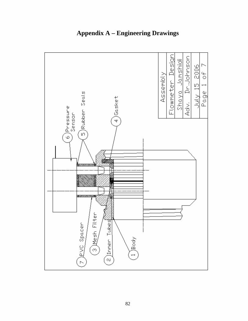
82
Appendix A – Engineering Drawings

83

84

85

86

87

88

89
Appendix B – Research Protocol
The Detection of Inhalation Flow Using Respiratory Protective Masks
Abstract: A key step in the proper design of respirators, as well as in the regulation of
occupational safety, is the determination of inhalation during exercise. A non-
invasive portable meter that detects average and peak inhalation is valuable step in
obtaining this overall goal. This meter will be attached externally to a military style
respirator mask (M-40A1). A study is being developed at the University of Maryland,
College Park that is working to achieve this goal. Results from such a study can be
used to determine the effectiveness of respirators in protecting individuals during
high intensity labor conditions.
Purpose: This project is intended to determine peak and average inhalation values
during exercise at a moderate exercise intensity of 80 % VO2max. Exercise at this
intensity will be completed once in a controlled laboratory environment, and a final
time outside under moderate environmental conditions.
1. Subject Selection:
a) Who will be the subjects, how will you persuade them to participate, and how
many do you expect to participate? If you plan to advertise for subjects,
please include a copy of the advertisement.
We plan to recruit 10 participants from the University of Maryland, College
Park. A portion of this sample will be drawn from a database stored in the
Human Performance Laboratory located in the Biological Resources
Engineering Department. Additional subjects will be selected through day-to-
day interaction within the campus community.
b) Will the subjects be selected for any specific characteristics (e.g. age, sex, race,
ethnic origin, religion, or any social or economical qualifications)?
We will be selecting subjects between the ages of 18-40 years.
c) State why the selection will be made on the basis or the bases given in 2(b)?

90
The selection criteria stipulated in 2(b) reflects a desire to recruit individuals
who are at minimal risk while taking part in vigorous physical activities.
Vigorous exercise may induce life-threatening cardiovascular responses in
older populations with known cardiovascular diseases; therefore, this group
may not be ideal for this project. The American College of Sports Medicine
(ACSM) in the Guidelines for Exercise Testing and Prescription (6th edition),
states that vigorous physical exercise is appropriate for asymptomatic
individuals between the ages of 18-40 years, and that medical clearance is not
required for this group prior to initiating a vigorous exercise program. This
project will not provide medical clearance for prospective participants, and as
a result, it is important to select individuals (aged 18-40 years) who do not
require medical clearance and are at minimal risk for cardiovascular events
while performing vigorous exercise.
2. Describe precisely what will be done to the subject.
Orientation
All participants will be asked to report for a one-hour orientation session. An
investigator will be present at this session to explain the test procedures and methods
applicable to this project. Volunteers will be provided with a written informed
consent document outlining these procedures and methods. Participants will be asked
to read and sign this document before being allowed to take part in this study.
Volunteers will be asked to complete several questionnaires. The first questionnaire
will be a brief medical history document designed to provide investigators with the
individual’s present and past health background as related to the study. Next, the
subject will be administered a Physical Activity Readiness Questionnaire (PAR-Q) to
determine whether exercise is appropriate at this time without first seeking medical
clearance. The American College of Sports Medicine, in the Guidelines for Exercise
Testing and Prescription, suggests administering this questionnaire to asymptomatic
individuals prior to instituting vigorous exercise programs. The medical history and
physical activity questionnaires will be used as screening tools to exclude individuals
who are at risk for cardiovascular events when performing vigorous physical
activities. The Spielberger State-Trait Anxiety Inventory will be the final
questionnaire administered to volunteers, providing investigators with information on
the individual’s present and general anxiety disposition. These questions provide
feedback on anxiety and are not intended to diagnose any psychological state.

91
All participants will be provided the opportunity to have any questions regarding this
study answered at this time or throughout the duration of the remaining test sessions.
Maximal Aerobic Capacity
All participants will undergo a maximal oxygen consumption assessment using a
Quinton motorized treadmill. First, participants will be allowed to warm-up on the
treadmill for approximately 5 minutes at 50-60% of his or her age-predicted
maximum heart rate, followed immediately by a brief stretching period. Next, the
volunteer will be seated and fitted with a Hans Rudolph breathing mask for the
collection of expiratory air. The test will begin with the treadmill speed and grade
gradually ramped to the desired work rate (50-60% age-predicted maximum heart rate
response) with this moment signifying the initial stage and lasting approximately 3
minutes. At the completion of this stage, a new work rate will be selected and the
participant will be required to work at this intensity for another 3 minutes. Work
rates will be modified every third minute during the maximal aerobic assessment
period. The session will be terminated If the participant fails to display a sufficient
rise in oxygen consumption rate (<150 ml/min) to correspond to the new work rate, If
the individual reaches his or her age-predicted maximal heart rate, If the individual
displays a response that contraindicates continued assessment (e.g. irregular EKG
tracings), or If the participant requests that the session be terminated. The maximal
aerobic assessment will last approximately 9-15 minutes.
A noninvasive Polar heart rate monitor will be used to assess heart rate responses
during the session.
Test Conditions
Participants will be asked to report to the lab on 2 separate days to exercise once on a
Quinton motorized treadmill at 80% of their maximal aerobic capacity as determined
by VO2max. On the second day, the subject will exercise at roughly this same
intensity outdoors, on Ludwig Field/Kehoe Track. Test sessions may or may not be
completed on consecutive days, as based on subject availability. Due to the weather
conditions, it may be necessary to run some of the tests on consecutive days. All of
the test will be done with the subject wearing a military-style respiratory mask with
an external flow meter attached. All tests will be run in the same manner, the only
difference being that in one test the subject is indoors on a treadmill, or outdoors on a

92
racetrack.
Test sessions will include warm-up or stretching periods directly prior to
commencement of the exercise. This is to ensure that the subject is adequately
prepared to exercise for a period without the risk of muscle injury or cardiovascular
abnormalities.
After arriving in the Human Performance Lab, subjects will be asked to start walking
on a treadmill for roughly five minutes as warm-up. Next they will be asked to
stretch their muscles for 5-10 minutes in an attempt to ensure that all their muscles
are properly stretched and that they are ready for exercise. The subjects will then be
fitted with a M40 military-style negative pressure respiratory mask with the attached
external flow meter that has been adjusted for standard conditions (contains the
standard filter). The indoor testing condition will be run on a treadmill at 0% grade
until volitional fatigue; only the speed of the treadmill belt will be adjusted to elicit
the specific work rate desired. The grade will be held constant during the exercise
tests for enhanced comparison and result interpretation. The speed of the treadmill
will be set to the appropriate level to elicit the specified work rate, and the treadmill
will be turned on while the subject is standing over the belt. Once outdoors, the
subject will be asked to maintain a particular speed based on previously obtained data
from their VO2max. Data logging and timing of the test will initiate once the subject
starts moving on belt, or on outdoor racing track. When the subject is no longer able
to proceed with the test as based on his or her fatigue level, data logging will stop, the
treadmill will be slowed before coming to a stop, and the time duration of the test will
be recorded. When outdoors, the subject can voluntarily stop moving as they please.
It is important to note that for all exercise tests, a short five minute cool-down period
will follow completion of the test to ensure subject safety and return to physical
control.
A Polar heart rate monitor will be used to provide heart rate responses during the
exercise sessions. Rating of Perceived Exertion and Breathing Apparatus Comfort
scales will be taken periodically during each test to provide investigators with
subjective feedback regarding the independent variables (e.g. exercise intensity and
subject-perceived mask comfort). Tests will be run at approximately the same time of
day in an attempt to ensure that physiological conditions are constant and any diurnal
cycles are not influencing the results obtained. All of the procedures listed above will

93
be employed for all exercise test sessions, namely all respiratory mask conditions
(with or without) and at all exercise intensities.
At 80% VO2max exercise intensities, it is anticipated that exercise will last
approximately 15-20 minutes. A single test condition, including the preparation time will last up to approximately 30-45 minutes; therefore, this project will necessitate that individuals commit roughly 2 hours to fulfill the requirements (1 orientation session with a maximal aerobic capacity test and 2 test conditions) outlined in this study. Participants are free to withdraw from this project at anytime without incurring a penalty. This request may be expressed to an investigator through verbal or written communication.
3. Risks and Benefits: Are there any risks to the subjects? If so, what are these
risks? What potential benefits will accrue to justify taking these risks?
Risks
Vigorous physical exercise may produce undesired cardiovascular responses in at-risk
populations, leading to possibly life-threatening situations. The medical history and
physical activity questionnaires will be used as screening tools to exclude this at-risk
group. An Automated External Defibrillator (AED) will be available for use should a
cardiovascular incident arise during test sessions. Investigators are trained and
certified in the use of the AED.
Benefits
Participants will not receive monetary benefits from taking part in this study;
however, individuals will be provided with test results upon completion of this
project.
Confidentiality
All participants will be assigned an identification number and will be referred to by
this descriptor in any presentation or publication of test findings. All files will be
stored and maintained in the assistant investigator’s office with access permitted to
only those individuals directly responsible for the collection and analysis of test data.
Information and Consent Form
An investigator will meet with each participant to explain the test procedures and
methods applicable to this project prior to the test date. The participant will be
provided with a written informed consent document outlining these procedures and

94
methods. Volunteers will be asked to read and sign this document before being
allowed to participate in the investigation.
Conflict of Interest
Investigators do not have a conflict of interest in this project.
HIPPA Compliance
This investigation will not be using protected health information. Identification
numbers will be assigned to help ensure the patient’s anonymity. Investigators plan
to adhere to the guidelines outlined by the University of Maryland at College Park
regarding any sensitive information.
Research Outside of the United States
a) Did the investigators previously conduct research in the country where the
research will take place? Briefly describe the Investigators’ knowledge and
experience working with the study population.
Not applicable. All research is taking place in the United States.
b) Are there any regulations, rules or policies for human subjects research in the
country where the research will take place? If so, please describe and explain
how you will comply with the local human subject protection requirements.
Not applicable. All research is taking place in the United States.
c) Do you anticipate any risks to the research participants in the country where the
research will take place, taking into account the population involved, the
geographic location, and the culture? If so, please describe. Risks could
include physical, psychological, social or economic risks. Do you anticipate
that subjects who participate in this research will be placed at risk of criminal or
civil liability? If so, please describe.
Not applicable. All research is taking place in the United States.
Research Involving Prisoners Not applicable. All research is being done using subjects from the University of
Maryland population and will not include prisoners.

95
Appendix C – Physical Activity Readiness Questionnaire
PAR-Q is designed to help you help yourself. Many health benefits are associated with regular
exercise, and the completion of PAR-Q is a sensible first step to take If you are planning to increase
the amount of physical activity in your life.
For most people, physical activity should not pose any problems or hazard. PAR-Q has been designed
to identify the small number of adults for whom physical activity might be inappropriate or those who
should have medical advise concerning the type of activity most suitable for them.
Common sense is your best guide in answering these few questions. Please read the carefully and
check YES or NO opposite the question If it applies to you. If yes, please explain.
YES NO
____ ____ 1. Has your doctor ever said you have heart trouble?
Yes, ______________________________________________________
____ ____ 2. Do you frequently have pains in your heart and chest?
Yes, ______________________________________________________
____ ____ 3. Do you often feel fain or have spells of severe dizziness?
Yes, ______________________________________________________
____ ____ 4. Has a doctor ever said your blood pressure was too high?
Yes, ______________________________________________________
____ ____ 5. Has your doctor ever told you that you have a bone or joint problem(s),
such as arthritis that has been aggravated by exercise, or might be made
worse with exercise?
Yes, ______________________________________________________
____ ____ 6. Is there a good physical reason, not mentioned here, why you should not
follow an activity program even If you wanted to?
Yes, ______________________________________________________
____ ____ 7. Are you over age 60 and not accustomed to vigorous exercise?
Yes, ______________________________________________________
____ ____ 8. Do you suffer from any problems of the lower back, i.e., chronic pain, or
numbness?
Yes, ______________________________________________________

96
____ ____ 9. Are you currently taking any medications? If YES, please specify.
Yes, ______________________________________________________
____ ____ 10. Do you currently have a disability or a communicable disease? If YES,
Please specify,
Yes, ______________________________________________________
If you answered NO to all questions above, it gives a general indication that you may participate in
physical and aerobic fitness activities and/or fitness evaluation testing. The fact that you answered NO
to the above questions, is no guarantee that you will have a normal response to exercise. If you
answered Yes to any of the above questions, then you may need written permission from a physician
before participating in physical and aerobic fitness activities and/or fitness evaluation testing at the
Deneka Fitness Center.
______________________ _____________________ _____________________
Print Name Signature Date
Please Note: If you contract a communicable disease, it is your responsibility to inform the staff of the
Clarkson University Fitness Center of this condition and your membership may be suspended until this
condition is cured or in a state of remission.

97
Appendix D – Program Code Front Panel

98
Block Diagram

99
Appendix E – Pressure Sensor Specifications Sheet

100

101
Appendix F – USB6009 Specifications Sheet

102
Appendix G – User Manual

103
Calibration Technique:
1. Connect Mask Flow Meter (MFM) (labeled 1) to the M40A1 respirator mask
and C2A1 filter.
2. Connect pressure transducer (labeled 2) to MFM body with the screws
provided.
3. Connect blue wire (labeled 3) to pressure traducer via the grey connecter
(labeled 4) ports highlighted.
4. Secure connector to wire with grey clip provided (labeled 5).
5. Connect wires to USB6009 (labeled 6).
6. Connect USB6009 to computer via a Universal Serial Bus (USB) port.
7. Place M40A1 mask to head form of breathing machine for dynamic data
calibration.
8. Set the parameters of the breathing machine to Profile of 3, Amplitude of 100.
9. Turn on the breathing machine and allow the machine to remain on for five
minutes prior to starting the simulated breathing cycles.
10. Turn on Computer
11. If you are using other programs, close all unrelated programs.
12. Select “MFM program” from program list and allow LabVIEW Program to
operate.
13. If physical channels are different from 0, please select physical channel.
14. If voltage input is different from + 5V, then set appropriate voltage range.
15. If sample rate is different from 50Hz, then set sample rate.
16. If sample mode is desired to be different from continuous, then set sample
mode.
17. If set sample scan mode is different from continuous, set sample scan mode.
18. If filtration mode is different from “smoothing”, set filtration mode.
19. Set file name path as desired.
20. Click on “run” to initiate the program.
21. Allow data to accumulate for thirty seconds.
22. Observe data on “Flow” chart.
23. Press “Stop” at anytime to terminate program.
24. Open Microsoft Excel program.
25. Open the file of data, saved in the location specified under file path name.
26. When the dialogue box opens, select “Finish” and the file path name will
open. Note: if the number 54728 data points, the duration of exercise time
must be saved under different file names to avoid truncation of data points.

104
27. Manipulate the data as needed, noting that the data is stored in separate
columns. Relative time is plotted in column one with units of seconds.
Voltage is plotted on the second column with units of Volts. Flow is plotted
in the second column with units of L/min.
28. Compare the voltage values observed from “standard” flow to the provided set
of values (labeled calibration data).
29. Plot the standard voltage values, x values, from calibration procedure against
the “standard” flow values, y values, in an excel chart.
30. Click on a data point, and select “add trend line” and select a “polynomial”
trend line with an order of 3.
31. Under the options tab, select display equation on chart. This will be the new
calibration equation.
32. Select the MFM program block diagram. Select “Formula” icon and insert the
calibration equation.
33. Save the program file. It is now ready for usage.
34. Calibrate the MFM system per ASTM
35. If any errors arise at any time, observe the error number, and determine the
error code at the National Instruments website www.ni.com.
User Manual Technique:
1. Connect Mask Flow Meter (MFM) (labeled 1) to the M40A1 respirator mask
and C2A1 filter.
2. Connect pressure transducer (labeled 2) to MFM body with the screws
provided.
3. Connect blue wire (labeled 3) to pressure traducer via the grey connecter
(labeled 4) ports highlighted.
4. Secure connector to wire with grey clip provided (labeled 5).
5. Connect wires to USB6009 (labeled 6).
6. Connect USB6009 to computer via a Universal Serial Bus (USB) port.
7. Turn on Computer
8. If you are using other programs, close all unrelated programs.
9. Select “MFM program” from program list and allow LabVIEW Program to
operate.
10. If physical channels are different from 0, please select physical channel.
11. If voltage input is different from + 5V, then set appropriate voltage range.

105
12. If sample rate is different from 50Hz, then set sample rate.
13. If sample mode is desired to be different from continuous, then set sample
mode.
14. If set sample scan mode is different from continuous, set sample scan mode.
15. If filtration mode is different from “smoothing”, set filtration mode.
16. Set file name path as desired.
17. Click on “run” to initiate the program.
18. Observe data on “Flow” chart.
19. Press “Stop” at anytime to terminate program.
20. Close LabVIEW program.
21. Open Microsoft Excel program.
22. Open the file of data, saved in the location specified under file path name.
23. When the dialogue box opens, select “Finish” and the file path name will
open. Note: if the number 54728 data points, the duration of exercise time
must be saved under different file names to avoid truncation of data points.
24. Manipulate the data as needed, noting that the data is stored in separate
columns. Relative time is plotted in column one. Flow is plotted in the
second column.
25. If any errors arise at any time, observe the error number, and determine the
error code at the National Instruments website www.ni.com.

106
Appendix H – VPBS Testing at Low and High Flow Rates Sample VPBS Instantaneous Flow versus Time:
VPBS High Flow - Run 1
-20
0
20
40
60
80
100
120
140
0 5 10 15 20 25 30 35
Relative Time (Seconds)
Insp
irat
ory
Flo
w (
L/m
in)
MFM FP Sample Data:
Breathing Machine RUN1 Breathing Machine RUN1
Low Flow Rate T-test Results for Average Inspiratory Flow
MFM FP t-Test: Two-Sample Assuming Unequal Variances
Breath VIavg PIF VIavg PIF
1 36.168 65.518 33.057 65.225 Variable 1 Variable 2
2 34.287 65.895 35.466 67 Mean 35.651809 35.478962
3 33.502 67.051 35.596 68.776 Variance 1.8387935 1.4362801
4 36.701 65.846 34.384 65.816 Observations 30 30
5 36.998 67.831 36.846 68.776 Hypothesized Mean Difference 0
6 36.9 67.718 36.579 68.184 df 57
7 35.958 65.302 34.645 65.225 t Stat 0.5231333
8 33.725 65.307 35.081 66.408 P(T<=t) one-tail 0.3014546
9 33.919 66.069 37.195 68.184 t Critical one-tail 1.6720289
10 34.399 66.112 36.253 67 P(T<=t) two-tail 0.6029093
11 35.058 65.895 35.507 67 t Critical two-tail 2.0024654

107
12 38.298 66.561 35.847 66.408
13 36.581 64.171 35.644 64.041 T-test Results for PIF
14 37.181 67.658 37.443 68.776 t-Test: Two-Sample Assuming Unequal Variances
15 34.461 67.094 35.249 68.776
16 33.902 65.677 35.081 67 Variable 1 Variable 2
17 36.954 65.216 33.631 65.225 Mean 65.846121 66.506959
18 35.574 65.067 33.827 65.816 Variance 1.2838078 2.152102
19 37.543 66.104 35.212 65.816 Observations 30 30
20 36.85 66.112 36.411 67 Hypothesized Mean Difference 0
21 35.756 64.904 34.843 64.041 df 55
22 36.406 67.546 37.24 68.184 t Stat -1.952696
23 36.311 65.017 33.008 64.633 P(T<=t) one-tail 0.0279761
24 36.059 64.783 34.747 65.225 t Critical one-tail 1.673034
25 35.963 66.519 35.673 66.408 P(T<=t) two-tail 0.0559522
26 35.462 64.148 37.492 65.816 t Critical two-tail 2.0040448
27 35.36 66.873 36.183 67.592
28 33.624 65.634 36.188 67
29 36.423 63.431 34.765 64.041
30 33.229 64.324 35.277 65.816
average 35.652 65.846 35.479 66.507
Breathing Machine RUN2
Low Flow Rate
MFM FP
Breath VIavg PIF VIavg PIF T-test Results for Average Inspiratory Flow
1 37.274 66.654 35.656 66.408
t-Test: Two-Sample Assuming Unequal
Variances
2 34.203 65.68 34.207 67
3 35.121 63.43 35.408 64.041 Variable 1
Variable
2
4 34.53 65.635 34.744 65.816 Mean 35.61133 35.14334
5 35.944 66.263 35.963 67 Variance 1.930656 1.892498
6 35.353 65.75 34.952 65.816 Observations 29 29
7 35.455 65.992 34.022 65.225 Hypothesized Mean Difference 0

108
8 35.984 66.783 36.326 67 df 56
9 35.166 66.108 35.925 66.408 t Stat 1.288911
10 35.126 65.171 35.602 65.816 P(T<=t) one-tail 0.101364
11 34.908 65.635 34.436 65.816 t Critical one-tail 1.672522
12 35.459 66.783 34.699 67 P(T<=t) two-tail 0.202728
13 34.62 65.287 34.807 65.816 t Critical two-tail 2.003241
14 33.923 61.063 32.442 61.082
15 34.814 64.457 31.993 63.449 T-test Results for PIF
16 33.753 65.964 33.264 66.408 t-Test: Two-Sample Assuming Unequal Variances
17 36.01 65.935 36.389 66.408
18 38.377 63.925 37.873 64.041 Variable 1
Variable
2
19 39.152 66.453 37.967 66.408 Mean 65.52474 65.77564
20 37.992 65.606 36.77 65.816 Variance 1.805052 2.150089
21 35.789 64.959 34.799 65.225 Observations 29 29
22 37.101 65.663 35.912 65.816 Hypothesized Mean Difference 0
23 35.371 63.741 33.677 63.449 df 56
24 35.311 64.988 34.953 65.225 t Stat -0.67938
25 36.379 67.787 35.668 68.184 P(T<=t) one-tail 0.249847
26 37.204 67.285 36.667 67.592 t Critical one-tail 1.672522
27 33.49 64.26 34.943 65.225 P(T<=t) two-tail 0.499695
28 34.454 66.61 34.56 67 t Critical two-tail 2.003241
29 34.465 66.35 34.532 67
average 35.611 65.525 35.143 65.776

109
Appendix I – Subject Testing at Rest and at 85% of Age Predicted Maximum Heart Rate Work Loads Sample VPBS Instantaneous Flow versus Time:
Subject #1 - At Rest
-5
0
5
10
15
20
25
30
0 10 20 30 40 50 60 70
Relative Time (seconds)
Insp
irat
ory
Flo
w (
L/m
in)
Smeter Fleisch Subject 1 - At Work Load of 85% Age Predicted Maximum Heart Rate
-30
0
30
60
90
120
150
180
210
240
270
0 10 20 30 40 50 60
Time (s)
Inst
anta
eno
us
Insp
irat
ory
Flo
w (
L/m
in)

110
Sample Data: Subject 1 At 85% Maximum Heart
Rate
Breath VI avg PIF
1 72.1872126 155.578153
2 77.7378253 152.460845
3 74.813698 145.528962
4 73.0688525 137.539294
5 71.2072288 121.795883
6 71.6079451 122.85178
7 81.7490635 130.91446
8 75.1344699 138.235163
9 91.756317 183.729311
10 55.9311488 154.539099
11 59.1239245 179.187195
12 107.761682 254.029442
13 63.7480195 135.10169
14 75.3363973 138.235163
15 52.4546657 111.170653
16 57.498847 133.3584
17 56.0155989 131.263848
18 46.651269 107.598227
19 55.5888319 110.814165
20 55.2941522 142.058347
21 51.6263801 112.594993
22 54.4241731 112.239146
23 59.7348091 125.662434
average 66.9761961 140.716811
Subject 1 At Rest
MFM FP
Breath VI avg PIF Vi avg PIF
1 12.604502 23.05783 13.512692 25.068351
2 10.764166 20.875121 11.561538 22.70092
3 11.573586 21.421922 12.419015 23.292778
4 9.8034781 21.783376 10.525008 23.68735
5 10.696072 22.139372 11.497902 24.081921
6 13.717211 22.504547 14.721643 24.476493
7 8.0448977 21.420201 8.6115671 23.292778
8 9.9053563 21.419228 10.624674 23.292778
9 8.5534122 22.507935 9.1647546 24.476493
10 9.0299149 22.492757 9.7218316 24.476493
11 10.622809 21.959266 11.419142 23.884636
12 8.5320633 20.872966 9.1398113 22.70092
13 7.7657969 20.873204 8.3191154 22.70092
14 6.7995825 21.422861 7.280486 23.297
15 9.9766927 21.414939 10.708586 23.292778
16 5.6804059 21.417951 6.0619052 23.294778
average 9.6293716 21.723967 10.330604 23.626087

111
Subject 2 At 85% Maximum Heart Rate
Breath Viavg PIF
1 55.353412 121.66938
2 53.839175 114.03458
3 48.095401 114.03458
4 43.566587 109.85796
5 50.386164 125.86688
6 60.140784 136.07012
7 54.013187 123.378
8 60.027938 124.9067
9 63.652406 132.49326
10 68.766208 136.07012
11 62.800452 126.05936
12 60.5704 126.44474
13 53.887085 119.59708
14 55.730754 125.09844
15 55.229074 134.87253
16 60.462639 133.87859
17 56.561132 122.23761
18 57.930139 126.63766
19 56.075429 121.10246
20 57.400152 118.101
21 56.88655 126.44474
22 57.579591 124.52365
average 56.770666 124.69907
Subject 2 At Rest
Prototype Fleisch
Breath VI avg PIF VI avg PIF
1 5.6038943 11.769323 5.2031033 12.829692
2 5.4551764 5.8250132 5.2989642 6.3357878
3 5.9998042 8.836987 5.8305494 9.739318
4 5.8977365 7.4712499 5.7082806 8.1635858
5 6.1589868 10.985016 5.7755635 11.943145
6 5.0571263 7.4162663 4.8384364 8.0874803
7 4.3098313 5.6821563 4.1302447 6.1730807
8 5.7724151 9.7845293 5.5079292 10.717409
9 6.6734282 13.837132 6.2280314 15.110677
10 5.8674961 10.607402 5.5385177 11.58047
11 6.0589098 11.061404 5.655326 12.009925
12 5.0418496 6.9806263 4.8590841 7.6317529
13 1.1288369 2.0069262 1.1259066 2.2568084
14 5.4876899 8.8447832 5.2173933 9.6470829
15 4.8052615 5.9692219 4.623707 6.4865527
average 5.2878962 8.4718691 5.0360692 9.2475179

112
Bibliography
American Thoracic Society. 1995. Standardization of Spirometry. American journal
of Respiratory & Critical Care Medicine 152: 1107-1136.
Babb, T., Tuner, N., Saupe, K., and Pawelczyk, J. 1989. Physical Performance During
Combinations of Hypercapnic, Resistive and Hot-air Breathing. American Industrial
Hygiene Association Journal 50:105-111.
Baker, R. 1988. An Introductory Guide to Flow Measurement. Oxford: Alden Press.
Beckwith, T., Buck, NL and Morgan, R. 1982. Mechanical Measurement Third
Edition. Redding: Addison Wesley Publishing Co.
Benchetrit, G. 2000. Breathing Pattern in Humans: Diversity and Individuality.
Respiratory Physiology 123-129.
Berndtsson, G. 2003. A New Simplified Technique for Measuring Inspiratory Flow
Characteristics. Journal of International Respiratory Protection 20:91-101.
Berndtsson, G. 2004. Peak Inhalation Air Flow and Minute Volumes Measured in a
Bicycle Ergometer Tests. Journal of ISRP 21:21-30.
Blackie, S., McElvaney, N., and Morrison, N. 1991. Normal Values and Ranges for
Ventilation and Breathing Pattern at Maximal Exercise. Chest 100:136-142.
Caretti, D., Coyne, K., Johnson, A., Scott, W., and Koh, F. 2001. Work Performance
When Breathing Through Different Respirator Inhalation and Exhalation Respiratory
Inhalation and Exhalation Resistance During Hard Work. Journal of Occupational
and Environmental Hygiene 3: 214-224.
Caretti D., and Whitely, J. 1998. Exercise Performance during Inspiratory Resistance
Breathing Under Exhaustive Constant Load Work. Ergonomics 41: 501-511.
Coyne, K., Caretti, D., Scott, W., Johnson, A., and Koh, F. 2006. Inspiratory Flow

113
Rates During Hard Work When Breathing Through Different Respirator Inhalation
and Exhalation Resistances. Journal of Occupational and Environmental Hygiene 3:
490-500.
Deno, N.S., Kamon, E., and Kaiser, D.M. 1981. Physiological Responses to
Resistance Breathing during short and prolonged exercise. American Industrial
Hygiene Association Journal 42: 616-623.
Doeblin, E.O. 1996. Fourth Edition Measurement Systems Application and Design.
New York: McGraw Hill Inc.
“Fleisch Pneumotacograph.” [Online] Available at
http://www.phippsbird.com/fleisch2.html (Accessed June 1, 2008)
Goldsmith, J. and Young, A. 1956. A New Type of Flow Resistor for Respiratory
Studies. 8:562-564.
Goldstein, R. 1996. Fluid Mechanics Measurements. Oxfod: Taylor & Francis.
Hansen, D. 1990. Chapter 14 pg 303 of The Work Environment. Volume 1.
Harper, P., Brown, CL., and Becks, J.G. 1991. Respirator Physiology Research:
Answers in Search of the Question. Journal of Occupation Medicine 33: 38-43.
Hayward, A.T.J. 1979. Flow meters. New York: Halsted Press.
Heus R., Den Hartog E., and Kistermaker L. 2004. Influence of Inspiratory
Resistance on Performance During Graded Exercise Tests on a Cycle Ergometer.
Applied Ergonomics 35:583-590.
Holmer, I. 2007. Minute Volume and Inspiratory Flow Rates During Exhaustive
Treadmill Walking Using Respirator. British Occupational Hygiene Society 51: 327-
335.
Holmer I., and Kuklane K. 2002. Respiratory Flow Patterns During Physical Work
with Respirators. National Institute for Working Life Research Report 2002:12.

114
Janssen L., Anderson N., Cassidy, P. et al. 2005. Interpretation of Inhalation Airflow
Measurements for Respirator Design and Testing. Journal of the International Society
for Respiratory Protection 22:122-141.
Johnson, A.T., and Cummings, E.G. 1975. Mask Design Considerations. American
Industrial Hygiene Association Journal 36:220-228.
Johnson, A.T. 1976. The Energetics of Mask Wear. American Industrial Hygiene
Association Journal 37(8): 479-488.
Johnson, A.T. 1999. Biological Process Engineering: An Analogical Approach to
Fluid Flow, Heat Transfer, and Mass Transfer Applied to Biological Systems. New
York: John Wiley & Sons, Inc.
Johnson, A.T. 1999. Effect of Respirator Inspiratory Resistance Level on a Constant
Load Treadmill Work Performance. American Industrial Hygiene Association
Journal. 60:474-479.
Johnson, A.T. 2006. Why Peak Flow Matters. Journal of International Society for
Respiratory Protection 23: 100-110.
Johnson, A.T., and Cummings, E. 1975. Mask Design Considerations. American
Industrial Hygiene Association Journal 36(3):220-228.
Johnson, A.T., Koh, F.C., et al. 2005. Inhalation Flow Rates During Strenuous
Exercise. Journal of International Society for Respiratory Protection 22:79-96.
Johnson, A.T., Mackey, K. et al. 2005. Exercise Performance While Wearing a Tight
Fitting Powered Air Purifying Respirator with Limited Flow. Journal of
Occupational and Environmental Hygiene 2:368-373.
Johnson, A.T., Scott, W.H. et al. 1997. Sweat Rate Inside a Full Face Piece
Respirator. American Industrial Hygiene Association Journal 58:881-894.
Johnson, A.T., Micelli, T.M., and Masitis, C. 1973. Flow Regimes in Protective

115
Masks. (Technical Report EATR 4712). Edgewood Arsenal, Md.: Department of the
Army, Directorate of Development and Engineering.
Kaufman, J.W. and Hastings, S. 2005. Respiratory Demand During Rigorous Physical
Work in a Chemical Protective Ensemble. Journal of Occupational and
Environmental Hygiene 2: 98-110.
Larson, K. 1994 Sizing Up Micro-machined Instruments. Controls 52.
Liptak, B.G. 1993. Flow Measurement. CRC Press
Marieb, E. and Hoehn, K. 2007. Human Anatomy & Physiology Seventh Edition. San
Francisco: Pearson Benjamin Cummings.
Maxfield, Mary. 1971. The Indirect Measurement of Energy Expenditure in Industrial
Situation. The American Journal of Clinical Nutrition 24:1126-38.
Miller, M.R., Pedersen, O.F., and Quanjer, P.H. 1998. The Rise and Dwell Time for
Peak Expiratory Flow in Patients With and Without Airflow Limitation. American
Journal of Respiratory Critical Care Medicine 158:23-27.
Miller, M.R., Pedersen, O.F., and Sigsgaard, T. 1997. Spirometry with a Fleisch
Pneumotachograph: Upstream Heat Exchanger Replaces Heating Requirements.
Journal of Applied Physiology 82: 1053-1057.
Miller, R.W., 1983. Flow Measurement Engineering Handbook. New York: McGraw
Hill Inc.
Miller, R.W., 1996. Flow Measurement Engineering Handbook Third Edition. New
York: McGraw Hill Inc.
Nikishikawq, T., Kobayashi, T., and Mikami et al. 1993. Intelligent Differential
Pressure Transmitter Using a Resonant Single Crystal Silicon Sensor. ISA
Ott, R.L., and Longnecker, M. 2001. An Introduction to Statistical Methods and Data
Analysis. PacIfic Grove: Duxbury.

116
Rebar, J., Johnson, A.T., Cohen, E., 2004. Effect of Differing Facial Characteristics
on Breathing Resistance Inside a Respirator Mask. Journal of Occupational and
Environmental Hygiene 1:343-348.
Roca, J et al. 1997. Clinical Exercise Testing with Reference to Lung Disease
indication, Standardizations and Interpretation Strategies. European Respirator
Journal 10:2662-89.
Saati, E. 2004. Dynamic Deadspace in Face Masks Used with Non-Invasive
Ventilators: a Lung Model Study. European Respirator 129-135.
Silver, L., Davidson, G., Janssen, D., et al. 1971. Analytical Modeling of Respiratory
Protective Devices. American Industrial Hygiene Association Journal 32(12): 775-
785.
Silverman, L., Robert, C.L., George, L., Drinker, K.R., and Carpenter, T.M. 1943.
Fundamental Factors in the Design of Protective Respiratory Equipment, Inspiratory
Air Flow Measurements on Human Subjects with and without Resistance. OSRD
report No.1222 Harvard School of Public Health, Boston MA.
Stocks, J., Sly, P., Tepper, R.S., and Morgan, W.J. Infant Respiratory Testing.
Published by John Wiley and Sons, 1996.
Stromberg, N.O., and Gronkvist, M.J. 1999. Improved Accuracy and Extended Flow
Range for a Fleisch Pneumotachograph. Medical and Biological Engineering &
Computing Journal 37: 456-460.
Tirimana, P., Herwaddrden, C. et al. 1996. Evaluation of the Suitability of Weekly
Peak Expiratory Flow Rate Measurements in Monitoring Annual Decline in Lung
Function Among Patients with Asthma and Chronic Bronchitis. British Journal of
General Practice 46:15-18.
Upp, E.L. 1993. Fluid Flow Measurement – A Practical Guide to Accurate Flow
Measurement. Houston: Gulf Publishing Company.

117
Yamashiro, S.M. and Grodins, F.S. 1971. Optimal Regulation of Respiratory Airflow.
Journal of Applied Physiology 30:597-602.
Yeh, M.P., Gardner, R.M., Adams, T.D., and Yanowitz, F.G. 1982. Computerized
determination of pneumotachometer characteristics using a calibrated syringe .
Journal of Applied Physiology 53:280-285.
Yeh, M.P., Adams, T.D., Gardner, R.M., and Yanowitz, F.G. 1984. Effect of O2, N2,
and CO2 composition on nonlinearity of FPCharacteristics. Journal of Applied
Physiology 56:1423-1425.
Zock, J. 1981. Linearity and Frequency Response of Fleisch Type
Pneumotachometer. European Journal of Physiology 391:345-352.


![[Drum] Bob Moses - Drum Wisdom](https://img.pdfslide.us/doc/110x75/577cbfd31a28aba7118e36ec/drum-bob-moses-drum-wisdom.jpg)