Design of a configurable LDPC decoder forhigh-speed wireless.

Miquel Esteve Martin

June 2012

1

Abstract

The proposed solution for a LDPC decoder according the IEEE 802.11nstandard is a multicode and multi rate solution, being capable to decode thecodes defined in it and also it can be reused, after adding extra blocks, todecode turbo codes for example defined in 3GPP standard.Moreover the proposed solution uses very low memory compared with otherexisting architectures, without a relevant penalty in terms of performanceand area, and has a very high throughput performance.

2

Acknowledgements

I would like to specially thank my supervisor Di Wu who help me a lotspecially at the begining when I dindn’t know how to focus a project likethis one. However after a deep study and reading a bunch of papers overand over, and the value advices of my supervisor always in the most criticalmoments when I was lost.I would also like to mention Eric Tell, because he gave me the oportunity towork at Coresonic AB, implementing my solution in a profesional enviroment.Before ending this section, I want to dedicate this thesis to my classmatesand also the friends I had over all those years of hard study Juanjo, Xavi,Roger, Alex, Tery, Santi and Cristina, as well as the swedish people I goalong well and really appreciate, therefore this thesis is also dedicated to youErilk Hagglund, Madeleine Englund, Per Fagrell and Bjorn Salang.

3

Contents

Contents . . . . . . . . . . . . . . . . . . . . . . . . . . . . . . . . . 4

1 Introduction and purpose of this work 7

2 LDPC codes 82.1 Introduction . . . . . . . . . . . . . . . . . . . . . . . . . . . . 82.2 TPMP algorithm . . . . . . . . . . . . . . . . . . . . . . . . . 92.3 Implementation contraints . . . . . . . . . . . . . . . . . . . . 11

3 Improved architecture 123.1 Introduction . . . . . . . . . . . . . . . . . . . . . . . . . . . . 123.2 Trellis topology . . . . . . . . . . . . . . . . . . . . . . . . . . 123.3 Efficient implementation of L(u1 ⊕ u2) . . . . . . . . . . . . . 153.4 Structured LDPC codes . . . . . . . . . . . . . . . . . . . . . 173.5 Soft-input soft-output concept . . . . . . . . . . . . . . . . . . 193.6 TDMP decoding algorithm . . . . . . . . . . . . . . . . . . . . 213.7 TPMP versus TDMP algorithm . . . . . . . . . . . . . . . . . 23

4 LDPC decoder architecture proposed 254.1 LDPC decoder performance . . . . . . . . . . . . . . . . . . . 254.2 LDPC decoder architecture . . . . . . . . . . . . . . . . . . . 274.3 Comparison with other architectures . . . . . . . . . . . . . . 324.4 Conslusions . . . . . . . . . . . . . . . . . . . . . . . . . . . . 364.5 Future work . . . . . . . . . . . . . . . . . . . . . . . . . . . . 36

A Throughput specifications 40

B Parity-check matrices definitions 42

4

List of Figures

1 Trellis graph representation for every check-node . . . . . . . . 132 g(x) = ln(1 + e−|x|) . . . . . . . . . . . . . . . . . . . . . . . . 163 Example of a matrix definition in IEEE 802.11n (Z = 27, R =

1/2) . . . . . . . . . . . . . . . . . . . . . . . . . . . . . . . . 174 Iterative soft-input soft-output . . . . . . . . . . . . . . . . . . 205 BER comparision using BP and TDMP algorithm . . . . . . . 236 FER comparision using BP and TDMP algorithm . . . . . . . 247 FER at 5 iterations, all code rates and 1944 bits . . . . . . . . 258 LDPC decoder architecture . . . . . . . . . . . . . . . . . . . 279 SISO unit architecture . . . . . . . . . . . . . . . . . . . . . . 2810 Dataflow for the i-th layer, and a single SISO unit . . . . . . . 2911 DFU schematic . . . . . . . . . . . . . . . . . . . . . . . . . . 3012 Permuter implementation . . . . . . . . . . . . . . . . . . . . 3113 LCW = 648, Z = 27 and R = {1/2, 2/3, 3/4, 5/6} . . . . . . . . 4214 LCW = 1296, Z = 54 and R = {1/2, 2/3, 3/4, 5/6} . . . . . . . 4315 LCW = 1944, Z = 81 and R = {1/2, 2/3, 3/4, 5/6} . . . . . . . 44

5

Glossary

LDPC (Low-Density Parity-Check)H (Parity-Check Matrix)Z (Permutation matrix size)R (Code rate)LCW (Codeword length)TPMP (Two-Phase Message-Passing)BP (Belief Propagation)SPA (Sum-Product Algorithm)LUT (Look-Up Table)TDMP (Turbo-Decoding Message-Passing)LLR (Log-Likelihood Ratio)APP (A Posteriori Probability)SISO (Soft-Input Soft-Output)BER (Bit Error Rate)FER (Frame Error Rate)PER (Packet Error Rate)DFU (Decoding Function Unit)BR (Barrel Shifter)MUX (Multiplexer)IFS (Inter-Frame Space)MCS (Modulation and Coding Scheme)GI (Guard Interval)Nss (Number of spatial streams)

6

1 Introduction and purpose of this work

This thesis is separated in three parts. The first one explains the basic con-cepts of LDPC codes, such as the grah representation of a code and the BP orTPMP decoding algorithm, as well as the problems to implement a randomLDPC codes.After this brief introduction to the basic concepts, an alternative representa-tion for an LDPC code is presented. This in combination with an the efficientserial computation of a parity operations, will allow the implementation ofthe check-node update messages with very efficient and small area withouta throughput, performance or area penalty. Additionally, a kind of pseudo-random or structured codes which are used in the standard are presented.This kind of codes turn the LDPC decoding problem into a turbo decodingproblem, and therefore a faster convergence speed is achieved. This sectionends explaining the TDMP decoding algorithm for structured LDPC codes.In the last section the proposed hardware architecture is described and com-pared with other existing architectures, proving that the proposed design inthis work is a good solution.

7

2 LDPC codes

2.1 Introduction

An LDPC code is a linear block code defined by a sparse parity-check matrixH = [hij]MxN , which can be represented by a bipartite graph. A low-densityparity-check matrix is tipically be very large, and as its name indicates thereare few ones randomly placed, which are spread out over the matrix. Inorder to show the bipartite graph representation for a parity-check matrix,a reduced matrix is proposed as an example, so condirering the followingparity-check matrix:

H =

1 1 1 1 0 0 0 01 0 1 1 1 0 0 00 0 0 1 1 1 0 10 0 0 0 1 1 1 1

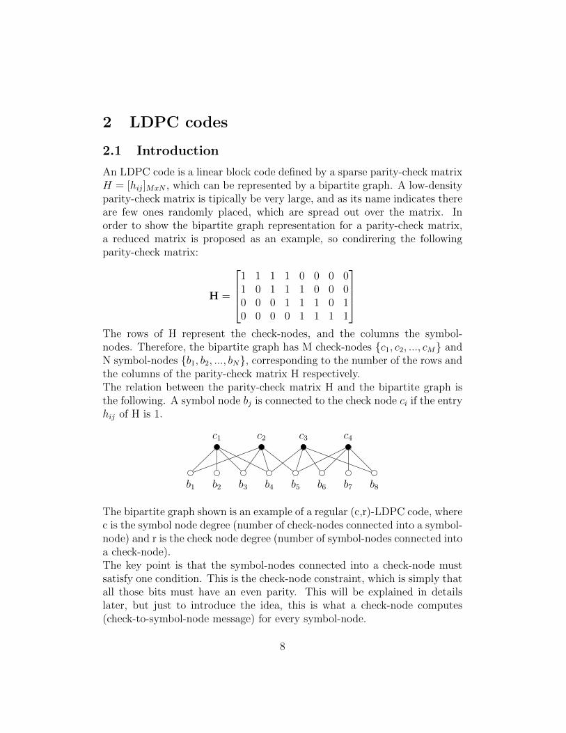
The rows of H represent the check-nodes, and the columns the symbol-nodes. Therefore, the bipartite graph has M check-nodes {c1, c2, ..., cM} andN symbol-nodes {b1, b2, ..., bN}, corresponding to the number of the rows andthe columns of the parity-check matrix H respectively.The relation between the parity-check matrix H and the bipartite graph isthe following. A symbol node bj is connected to the check node ci if the entryhij of H is 1.

c1 c2 c3 c4

b1 b2 b3 b4 b5 b6 b7 b8

The bipartite graph shown is an example of a regular (c,r)-LDPC code, wherec is the symbol node degree (number of check-nodes connected into a symbol-node) and r is the check node degree (number of symbol-nodes connected intoa check-node).The key point is that the symbol-nodes connected into a check-node mustsatisfy one condition. This is the check-node constraint, which is simply thatall those bits must have an even parity. This will be explained in detailslater, but just to introduce the idea, this is what a check-node computes(check-to-symbol-node message) for every symbol-node.

8

2.2 TPMP algorithm

The TPMP algorithm (Two-Phase Message-Passing Algoritm), also knownas BP (Belief Propagation) or SPA (Sum-Product Algorithm), is describedin this section. Basically, it consist in two types of messages between thesymbol-nodes and the check-nodes (symbol-to-check-node messages and check-to-symbol-node messages).

Then taking into account the trellis structure of a LDPC matrix HMxN , andconsidering the transmitted codeword u = [u1, ..., uN ], and the recieved code-word y = [y1, ..., yN ], the following notation is introduced before to presentformally the decoding algorithm:

M(n) set of check-nodes connected to the symbol-node nM(n)\m excluding the m-th check-nodeN (m) set of symbol-nodes connected to the the check-node mN (m)\n excluding the n-th symbol-nodeλn→m(un) symbol-node to check-node messageΛm→n(un) check-node message to symbol-node

Before explaining the meaning of λn→m(un) and Λm→n(un), must be definedthe LLR (log-likelihood ratio) of a binary random variable U = {0,1}, thisis:

L(U) = ln

(P (U = 0)

P (U = 1)

)(1)

Then, knowing that qn→m(x) is the message that the symbol-node n sendsto check-node m indicating the probability of being 0 or 1 of symbol n andrm→n(x) the message from check-node m to symbol node n indicating theprobability of symbol n being 0 or 1, the meaning of λn→m(un) and Λm→n(un),will be clarified. Both are defined as the LLR as follows:

λn→m(un) = ln

(qn→m(0)

qn→m(1)

)(2)

Λm→n(un) = ln

(rm→n(0)

rm→n(1)

)(3)

9

Then the formal desciption of the TPMP algorithm in log domain consistin the following steps:

Step 0) InitializationFirst of all the symbol-node are initialised to the recieved soft bits. Thereforethe symbol-to-check node and the check-to-symbol node are:

λn→m(un) = L(un)

Λm→n(un) = 0

Step 1) Check-node update ∀m,n ∈ N (m)The check-nodes generates the incremental soft information for every symbol-node, computing the check-node constraint. This is what the following ex-pression means:

Λm→n(un) = 2 · tanh−1

{ ∏n′∈N (m)\n

tanh

(λn′→m(u′n)

2

)}(4)

Step 2) Symbol-node update ∀n,m ∈M(n)Every check-node recieves the check-to-symbol-node messages, and adds thisincremental information to the recieved soft bits:

λn(un) = L(un) +∑

m∈M(n)

Λm→n(un) (5)

Then the symbol-to-check-node message is calculated to start a new decodingiteration. At this point, one decoding iteration has been completed, whichmeans that steps 1 and 2 will be executed as many times as desired decodingiterations.

λn→m(un) = L(un) +∑

m′∈M(n)\m

Λm′→n(un) (6)

Step 3) Hard decisionWhen the final decoding iteration is reached, is time for the hard decision ofthe symbol-nodes information. Going back to the LLR definition, it’s easyto see that, the hard decision consist in taking the sign bits of each soft bit.

un =

{0 if λn(un) ≥ 01 if λn(un) < 0

10

2.3 Implementation contraints

The implementation of the TPMP algorithm of randomly constructed LDPCcodes implies an important hardware complexity in terms of interconnect andmemory overhead.One possible way to do that, is implementing the bipartite graph, this is a setof symbol-nodes and check-nodes, and interconnect them. Due the randomstructure of the parity-check matrix, the interconnection between the nodesis random too. Therefore, for a large number of symbol and check-nodes theinterconnection problem becomes significant, in terms of placement, routingand timing. This can be, approximately, only for routing a chip area usagearound 50%.It is also possible to communicate the symbol and check-nodes through mem-ories instead of through an interconnection matrix, an then saving the ran-dom interconnection problem. Unfortunately, using this technique a largememory overhead will be required.

11

3 Improved architecture

3.1 Introduction

In this section, a new way to compute the check-node operations will be intro-duced, as well as an efficient hardware implementation for those operations.This is performed by using an alternative representation for the bipartitegraph, also referred as the trellis graph representation.Additionally, the structured codes (turbo-like codes) will be presented, whichavoids the randomness of the conventional codes, will turn the LDPC decod-ing problem into a turbo-decoding problem. This kind of codes, are definedand used in the IEEE 802.11n standard, so the archiecture proposed will tryto achieve an efficient implementation to be used as a decoder for that stan-dard. Moreover, the turbo-decoding algorithm for LDPC codes, or TDMPalgorithm (Turbo-Decoding Message-Passing algorithm) will converge faster,as it will be explained later on.To sum up, the theoretical background concepts to understand an efficientarchitecture for the IEEE 802.11n, will be exposed, as well as the TDMPalgorithm. Once this concepts are explained, the reader will be able to un-derstand the proposed architecture.

3.2 Trellis topology

There is an alternative representation for an LDPC code instead of the bi-partite graph. Taking into account that the j-th row of HMxN , has dc onesat postitions {j1, ..., jc}, then taking the bits {uj1 , ...ujc} of the codeword uwill have to satisfy the parity-check constraint of each row has to have evenparity:

uj1 ⊕ uj2 ⊕ ...⊕ ujc = 0 (7)

If the LLR values are used, the parity-check constraint can be expressed as:

L(uj1 ⊕ uj2 ⊕ ...⊕ ujc) = 0 (8)

This is also expressed using the boxplus or Hagenhauer’s opeator � as:

L(uj1) � L(uj2) � ...� L(ujc) = 0 (9)

In other words, all elements connected to a check-node will have to satisfy aneven parity. Then the trellis representation for every a check-node (Figure 1)

12

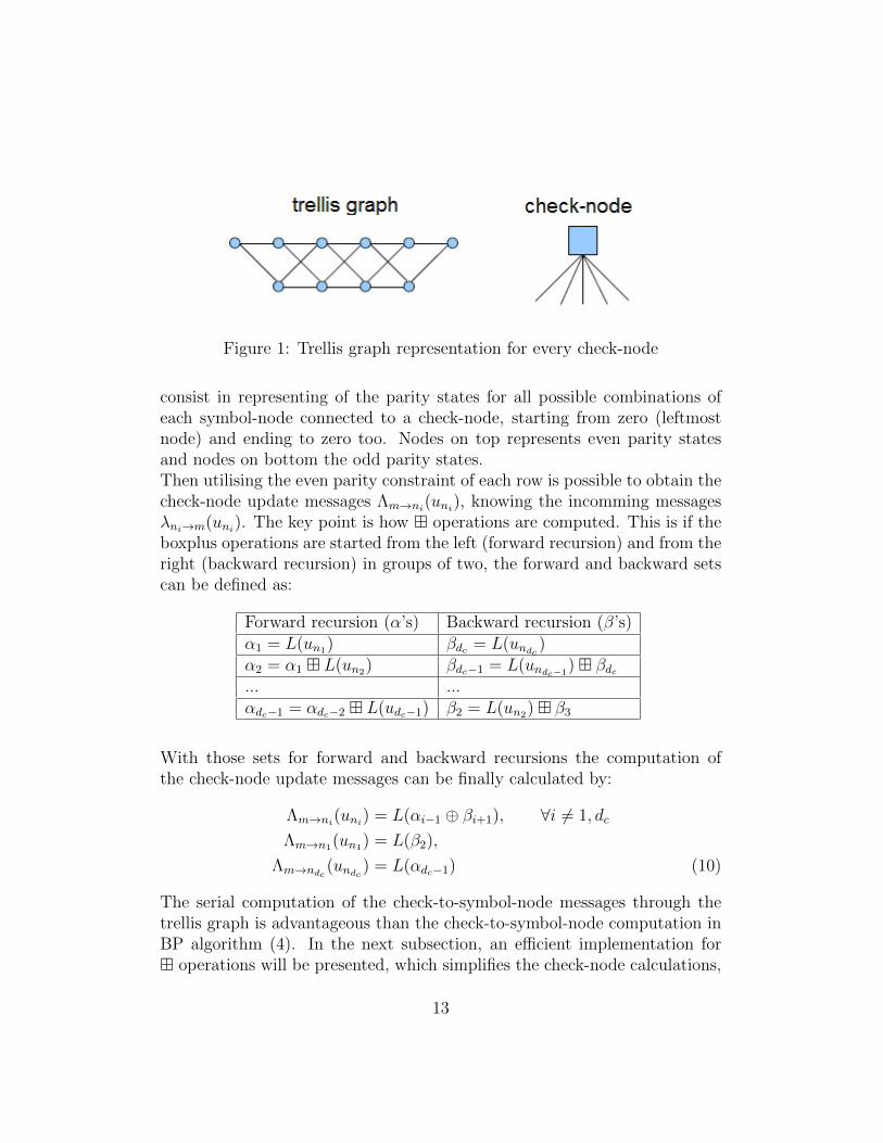
Figure 1: Trellis graph representation for every check-node

consist in representing of the parity states for all possible combinations ofeach symbol-node connected to a check-node, starting from zero (leftmostnode) and ending to zero too. Nodes on top represents even parity statesand nodes on bottom the odd parity states.Then utilising the even parity constraint of each row is possible to obtain thecheck-node update messages Λm→ni(uni), knowing the incomming messagesλni→m(uni). The key point is how � operations are computed. This is if theboxplus operations are started from the left (forward recursion) and from theright (backward recursion) in groups of two, the forward and backward setscan be defined as:

Forward recursion (α’s) Backward recursion (β’s)α1 = L(un1) βdc = L(undc )α2 = α1 � L(un2) βdc−1 = L(undc−1

) � βdc... ...αdc−1 = αdc−2 � L(udc−1) β2 = L(un2) � β3

With those sets for forward and backward recursions the computation ofthe check-node update messages can be finally calculated by:

Λm→ni(uni) = L(αi−1 ⊕ βi+1), ∀i 6= 1, dc

Λm→n1(un1) = L(β2),

Λm→ndc (undc ) = L(αdc−1) (10)

The serial computation of the check-to-symbol-node messages through thetrellis graph is advantageous than the check-to-symbol-node computation inBP algorithm (4). In the next subsection, an efficient implementation for� operations will be presented, which simplifies the check-node calculations,

13

compared with the two hyperbolic tangents that must be carried out in (4),that implies using a LUT for tanh and its inverse, becoming significant whenrepresenting a wide range of values.Moreover, a compact hardware implementaion will be introduced through asimple aproximation. Later on will also shown that its performance is veryclose to the floating point case, and at the end of the report, a comparisionwith other hardware architectures will be done, proving that the proposedsolution stands out in many aspects, and this will imply a reduced core area.

14

3.3 Efficient implementation of L(u1 ⊕ u2)The trellis representation of a LDPC code was presented in the previoussection, and was exposed how Λm→ni(uni) can be expressed as LLR of theXOR of forward and backward recursion L(αi−1 ⊕ βi+1). In this section, anefficient computation of XOR operations will be presented.Let’s start from the formal definition of L(u1⊕ u2). It can be demonstrated,that for statistically and independent random variables u1 and u2:

L(u1 ⊕ u2) ≡ L(u1) � L(u2)

L(u1 ⊕ u2) = ln

(1 + eL(u1) · eL(u2)

eL(u1) + eL(u2)

)(11)

Note that:L(u) �±∞ = ∓∞ and L(u) � 0 = 0

In order to reduce the computation complexity of L(u1 ⊕ u2) the expressionwill be aproximated. First of all, rewriting the :

L(u1 ⊕ u2) = ln(1 + eL(u1) · eL(u2))− ln(eL(u1) + eL(u2))

The following expression for L(u1⊕u2) is purposed in [10], using the Jacobianalgorithm for the numerator and the denominator obtaining:

L(u1 ⊕ u2) = max(0, L(u1) + L(u2)) + ln(1 + e−|L(u1)+L(u2)|)

− max(L(u1), L(u2))− ln(1 + e−|L(u1)−L(u2)|) (12)

where the Jacobian algorithm approximates this expression:

f(x, y) = ln(ex + ey) (13)

to the following one:

f(x, y) ≈ max(x, y) + ln(1 + e−|x−y|) (14)

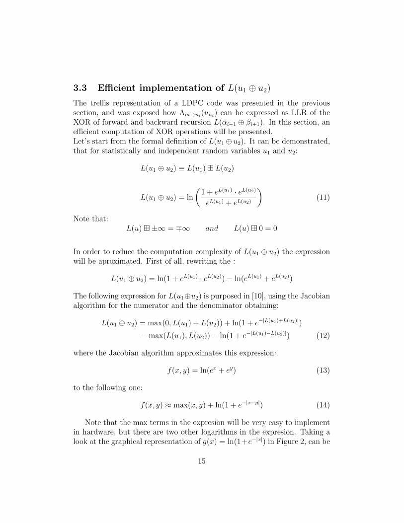
Note that the max terms in the expresion will be very easy to implementin hardware, but there are two other logarithms in the expresion. Taking alook at the graphical representation of g(x) = ln(1+e−|x|) in Figure 2, can be

15

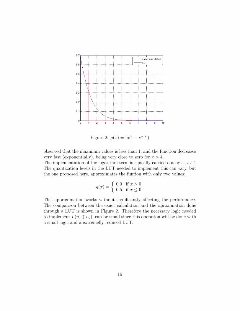
Figure 2: g(x) = ln(1 + e−|x|)

observed that the maximum values is less than 1, and the function decreasesvery fast (exponentially), being very close to zero for x > 4.The implementation of the logarithm term is tipically carried out by a LUT.The quantization levels in the LUT needed to implement this can vary, butthe one proposed here, approximates the funtion with only two values:

g(x) =

{0.0 if x > 00.5 if x ≤ 0

This approximation works without significantly affecting the performance.The comparison between the exact calculation and the aproximation donethrough a LUT is shown in Figure 2. Therefore the necessary logic neededto implement L(u1⊕u2), can be small since this operation will be done witha small logic and a extremelly reduced LUT.

16

Figure 3: Example of a matrix definition in IEEE 802.11n (Z = 27, R = 1/2)

3.4 Structured LDPC codes

As it was introduced before, the random structure of the parity-check matriximplies an implementation challenge. However, another kind of parity-checkmatrices can be used, pseudo-randomly constructed, with a BER permor-mance close to random-constructed codes. This are called structured codes.A structured LDPC code, consist in decomposing the parity-check matrixHMxN in smaller ZxZ submatrices, having n = N/Z block columns, andm = (1−R) ·n block rows. The ZxZ submatrices can be the idendty matrixshifted a certain number of positions, or a null matrix.The IEEE defines three different codeword lengths, as well as four differentcode rates for each codeword. Note that the number of block columns is fixedto 24 for all parity-check matrices in the standard, therefore:

Codeword (bits) Z Code rate (R)648 27 1/2, 2/3, 3/4, 5/61296 54 1/2, 2/3, 3/4, 5/61944 81 1/2, 2/3, 3/4, 5/6

This codes have the advantage of a hardware-efficient implementation, anda very compact definition, which means that can be stored using a relativesmall memory. This is easy to see taking a look at one parity-check matrixdefinition in the standard (Figure 3), only the ZxZ matrices have been rep-resented, indicating the number of positions that the idendity matrix has tobe rotated, or “-1” to denote a null ZxZ matrix.By the other hand, having the parity-check matrix decomposed into dif-ferent block rows (equivalent to supercodes for turbo codes), which can be

17

viewed as a concatenation of m submatrices, and the trellis representationof an LDPC code, can turn the LDPC decoding problem into a turbo de-coding problem. Therefore a new decoding algorithm, known as TDMP(Turbo-Decoding Message-Passing) algorithm will be used to decode struc-tured LDPC codes.Viewing the parity-check matrix as a turbo-like code, have some advantages.First of all, the communication between adjacent supercodes is done throughan interleaver or permuter. Taking into account that the non-zero ZxZ sub-matrices are the idendity matrix shifter a certain number of positions insteada random submatrix, the permuter becomes simply in a barrel shifter.Additionally, another advantage of this turbo-like codes is that the Turbo-Decoding Message-Passing algorithm converges faster than the traditionalalgorithm.These concepts will be probably understood better when the TDMP algo-rithm is explained, later on.

18

3.5 Soft-input soft-output concept

For communications engineering, the Baye’s theorem [14] is very useful forhypotesis testing, and estimate the probability of the transmited data whenan AWGN channel may corrupt the information. Then, considering the trans-mited data ‘d’ and the recieved data plus noise ‘x’ (continous and observablevalue):

P (d = i|x) =p(x|d = i)P (d = i)

p(x)(15)

where:

P (d = i|x) represents the a posteriori probability (APP).p(x|d = i) is the probability density function of the continous-valued data-plus-noise signal ‘x’.P (d = i) is the a priori probability.p(x) is the probability density function of the recieved signal ‘x’.

and ‘i’ is a set of M classes, but taking into account the binary case fora BSPK modulation i = {-1,+1}.

Once this was introduced, if the LLR definition is applied to the Baye’srule, and L′(d) is used to denote the LLR of the APP:

L′(d) = ln

(P (d = +1|x)

P (d = −1|x)

)Then the LLR of the Baye’s rule, the APP can be expressed as an additionof LLR, therefore the soft decision out of a detector is shown in the followingequation as:

L(d|x) = L(x|d) + L(d) (16)

L′(d) = Lc(x) + L(d) (17)

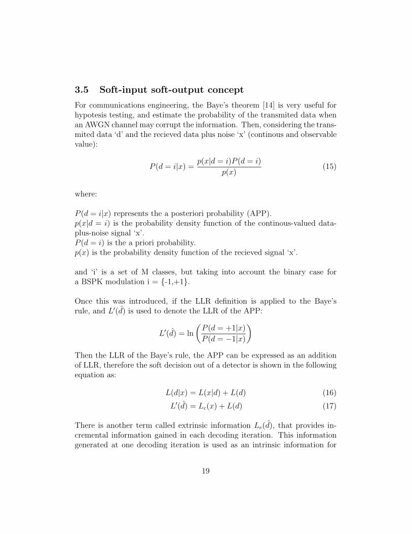
There is another term called extrinsic information Le(d), that provides in-cremental information gained in each decoding iteration. This informationgenerated at one decoding iteration is used as an intrinsic information for

19

Figure 4: Iterative soft-input soft-output

the next decoding iteration. Then considering extrinsic information, theAPP LLR is:

L(d) = Lc(x) + L(d) + Le(d) (18)

Note that assuming an AWGN channel, the LLR channel value or Lc(x) iscalculated as:

Lc(x) = ln

(p(x|d = +1)

p(x|d = −1)

)= ln

(1

σ·√2πe{−

12·(x−1

σ)2}

1σ·√2πe{−

12·(x+1

σ)2}

)=

2 · xσ

The iterative siso decoding scheme is ilustrated in Figure 4. For the firstdecoding iteration the data is supposed to be equally likely, and thereforeL(d) = 0. After every decoding iteration the extrinsic information generatedis going to be used as a priori information for the next iteration.

20

3.6 TDMP decoding algorithm

Once the soft decodig was introduced, the turbo decoding principle is goingto be used to decode LDPC codes. This algorithm is described in [2] and [3].Before exposing the algorithm, the notation will be presented. Taking intoaccount the soft decoding parameters introduced in the previous section, thisis the a priori and channel value as inputs, and extrinsic and posterior mes-sage as outputs, will be denoted as:

- Recieved channel LLR value δ.- A priori or intrinsic information λ.- Extrinsic information Λ.- Output posterior messages Γ.

Additionally Πi and Π−1i will be used to denote the permutation and in-verse permutation of a full block row. That means that the LLR values willbe sorted according to the permutation matrices in H. The way to do it isthe following. Consider the j-th block row of the LDPC matrix H, with cpermutation matrices {Πj1, ...,Πjc} in that block row of size SxS, where eachpermutation matrix is a ciclic permutation of the identity matrix. Then if SLLR messages have to be permuted according to one of those permutationmatrices, implies that Πji operation will perform a circular left shift and Π−1jia circular right shift as much as the permutation matrix indicates.After introducing the notation, the algorithm will be presented below, andconsist in the following 3 steps.1) First fo all, the posterior memory γ is initialized to the recieved channelvalue δ the intrinsic memory λ is set to zero.

γ = δ

After the initialization, the steps 2 and 3 are going to be done for all con-stituent codes in the LDPC matrix HMxN , from i = 1 to D to complete onedecoding iteration, where D is the number of block rows in HMxN .2) Then the decoder input is computed as the following equation states. Notethat in order to avoid the correlation between the messages the λi is sub-tracted. This is the same that was done in the TPMP algorithm to computethe symbol to check-node update messages.

ρ = Πi(γ)− λi

21

3) Finally, the SISO decoder generates the extrinsic message output Λi. Thisis going to be used at the next iteration as an intrinsic information, and ther-fore it is written back to the intrinsic memory replacing the old intrinsic valueλi. The decoder output is also used to generate the posterior information Γ,which is going to be written back to the posterior memory γ.

Γ = ρ+ Λi

γ = Π−1i (Γ)

When steps 2 and 3 are done for all block rowsm this is D time, a singledecoding iteration is completed. After that, it can be done for a certainnumber of iterations.

22

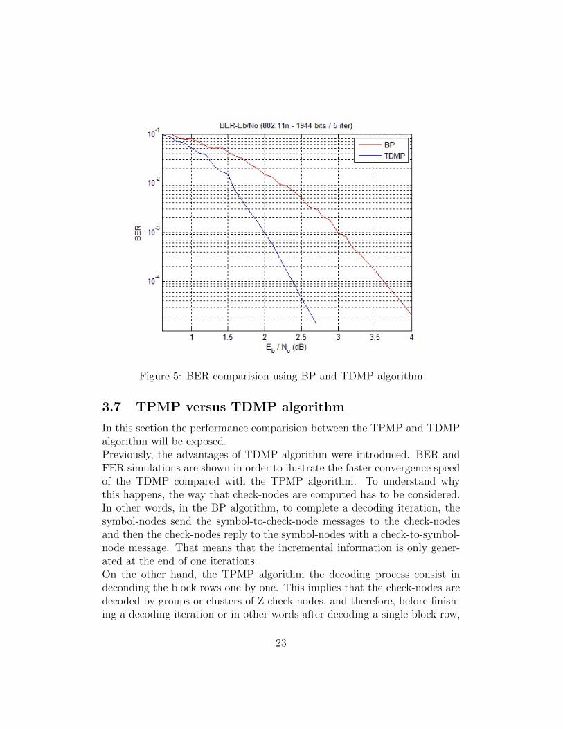
Figure 5: BER comparision using BP and TDMP algorithm

3.7 TPMP versus TDMP algorithm

In this section the performance comparision between the TPMP and TDMPalgorithm will be exposed.Previously, the advantages of TDMP algorithm were introduced. BER andFER simulations are shown in order to ilustrate the faster convergence speedof the TDMP compared with the TPMP algorithm. To understand whythis happens, the way that check-nodes are computed has to be considered.In other words, in the BP algorithm, to complete a decoding iteration, thesymbol-nodes send the symbol-to-check-node messages to the check-nodesand then the check-nodes reply to the symbol-nodes with a check-to-symbol-node message. That means that the incremental information is only gener-ated at the end of one iterations.On the other hand, the TPMP algorithm the decoding process consist indeconding the block rows one by one. This implies that the check-nodes aredecoded by groups or clusters of Z check-nodes, and therefore, before finish-ing a decoding iteration or in other words after decoding a single block row,

23

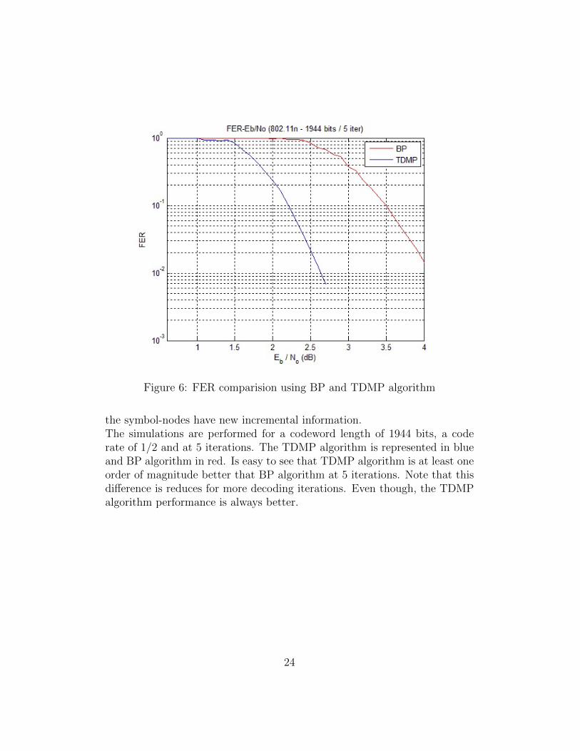
Figure 6: FER comparision using BP and TDMP algorithm

the symbol-nodes have new incremental information.The simulations are performed for a codeword length of 1944 bits, a coderate of 1/2 and at 5 iterations. The TDMP algorithm is represented in blueand BP algorithm in red. Is easy to see that TDMP algorithm is at least oneorder of magnitude better that BP algorithm at 5 iterations. Note that thisdifference is reduces for more decoding iterations. Even though, the TDMPalgorithm performance is always better.

24

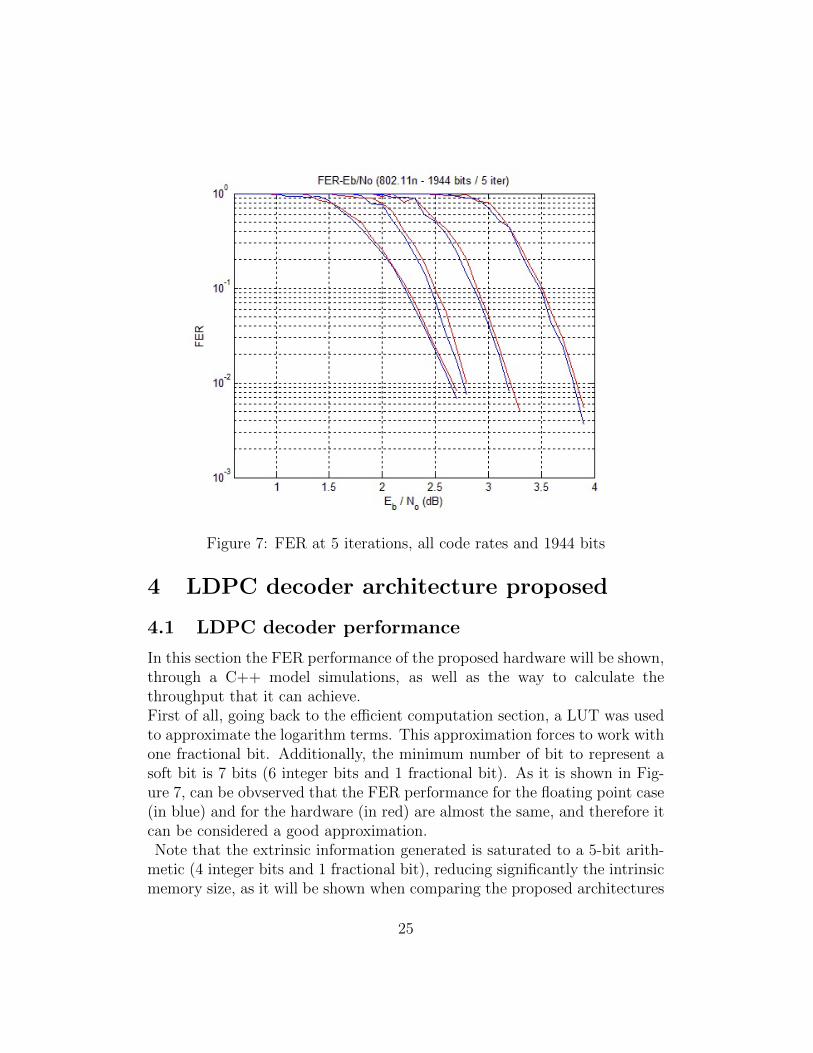
Figure 7: FER at 5 iterations, all code rates and 1944 bits

4 LDPC decoder architecture proposed

4.1 LDPC decoder performance

In this section the FER performance of the proposed hardware will be shown,through a C++ model simulations, as well as the way to calculate thethroughput that it can achieve.First of all, going back to the efficient computation section, a LUT was usedto approximate the logarithm terms. This approximation forces to work withone fractional bit. Additionally, the minimum number of bit to represent asoft bit is 7 bits (6 integer bits and 1 fractional bit). As it is shown in Fig-ure 7, can be obvserved that the FER performance for the floating point case(in blue) and for the hardware (in red) are almost the same, and therefore itcan be considered a good approximation.Note that the extrinsic information generated is saturated to a 5-bit arith-

metic (4 integer bits and 1 fractional bit), reducing significantly the intrinsicmemory size, as it will be shown when comparing the proposed architectures

25

with other existing designs.Then, knowing that the number of cycles needed to compute one block row istwo times the check-node degree, a single iteration needs to decode m blockrows, the throughput can be expressed with the following formula:

Θ =Lcw ·R · fclk

Niter · 2 ·∑m

i=1 ci(19)

where:Lcw is the codeword length.R is the code rate.fclk is the clock frequency.Niter is the number of decoding iterations performed.2 · ci are the cycles to decode a block row (ci is the check-node degree).∑m

i=1 ci is the addition all block row check-node degree.

Note that the latency (in cycles), is:

` = Niter · 2 ·m∑i=1

ci (20)

Lcw (bits) Code rate∑m

i=1 ci648 1/2, 2/3, 3/4, 5/6 88, 88, 88, 881296 1/2, 2/3, 3/4, 5/6 86, 88, 88, 851944 1/2, 2/3, 3/4, 5/6 86, 88, 85, 79

26

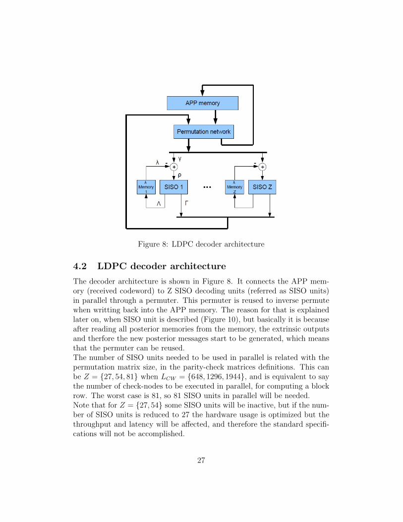
Figure 8: LDPC decoder architecture

4.2 LDPC decoder architecture

The decoder architecture is shown in Figure 8. It connects the APP mem-ory (received codeword) to Z SISO decoding units (referred as SISO units)in parallel through a permuter. This permuter is reused to inverse permutewhen writting back into the APP memory. The reason for that is explainedlater on, when SISO unit is described (Figure 10), but basically it is becauseafter reading all posterior memories from the memory, the extrinsic outputsand therfore the new posterior messages start to be generated, which meansthat the permuter can be reused.The number of SISO units needed to be used in parallel is related with thepermutation matrix size, in the parity-check matrices definitions. This canbe Z = {27, 54, 81} when LCW = {648, 1296, 1944}, and is equivalent to saythe number of check-nodes to be executed in parallel, for computing a blockrow. The worst case is 81, so 81 SISO units in parallel will be needed.Note that for Z = {27, 54} some SISO units will be inactive, but if the num-ber of SISO units is reduced to 27 the hardware usage is optimized but thethroughput and latency will be affected, and therefore the standard specifi-cations will not be accomplished.

27

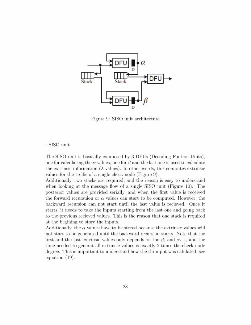
Figure 9: SISO unit architecture

- SISO unit

The SISO unit is basically composed by 3 DFUs (Decoding Funtion Units),one for calculating the α values, one for β and the last one is used to calculatethe extrinsic information (λ values). In other words, this computes extrinsicvalues for the trellis of a single check-node (Figure 9).Additionally, two stacks are required, and the reason is easy to understandwhen looking at the message flow of a single SISO unit (Figure 10). Theposterior values are provided serially, and when the first value is receivedthe forward recursuion or α values can start to be computed. However, thebackward recursion can not start until the last value is recieved. Once itstarts, it needs to take the inputs starting from the last one and going backto the previous recieved values. This is the reason that one stack is requiredat the begining to store the inputs.Additionally, the α values have to be stored because the extrinsic values willnot start to be generated until the backward recursion starts. Note that thefirst and the last extrinsic values only depends on the β2 and αc−1, and thetime needed to generat all extrinsic values is exactly 2 times the check-nodedegree. This is important to understand how the throuput was calulated, seeequation (19).

28

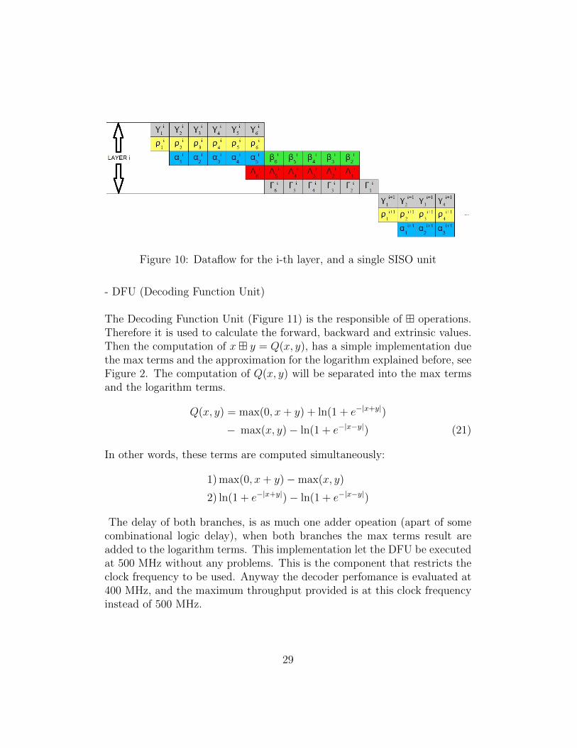
Figure 10: Dataflow for the i-th layer, and a single SISO unit

- DFU (Decoding Function Unit)

The Decoding Function Unit (Figure 11) is the responsible of � operations.Therefore it is used to calculate the forward, backward and extrinsic values.Then the computation of x� y = Q(x, y), has a simple implementation duethe max terms and the approximation for the logarithm explained before, seeFigure 2. The computation of Q(x, y) will be separated into the max termsand the logarithm terms.

Q(x, y) = max(0, x+ y) + ln(1 + e−|x+y|)

− max(x, y)− ln(1 + e−|x−y|) (21)

In other words, these terms are computed simultaneously:

1) max(0, x+ y)−max(x, y)

2) ln(1 + e−|x+y|)− ln(1 + e−|x−y|)

The delay of both branches, is as much one adder opeation (apart of somecombinational logic delay), when both branches the max terms result areadded to the logarithm terms. This implementation let the DFU be executedat 500 MHz without any problems. This is the component that restricts theclock frequency to be used. Anyway the decoder perfomance is evaluated at400 MHz, and the maximum throughput provided is at this clock frequencyinstead of 500 MHz.

29

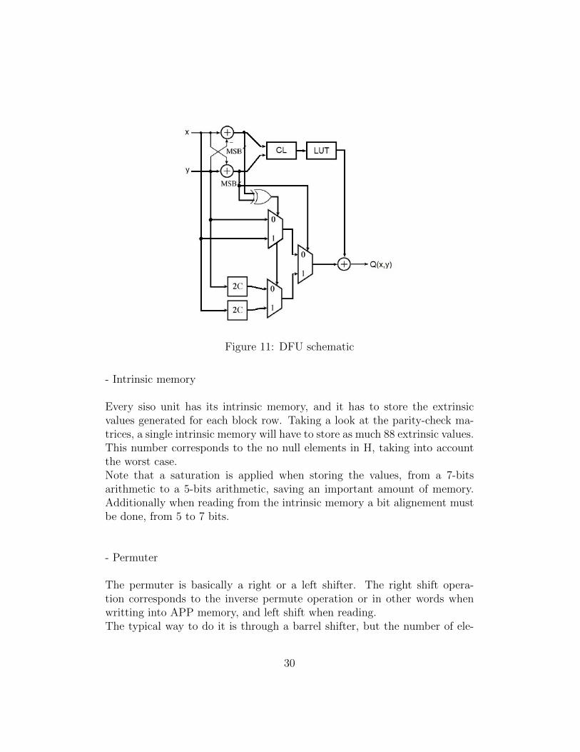
Figure 11: DFU schematic

- Intrinsic memory

Every siso unit has its intrinsic memory, and it has to store the extrinsicvalues generated for each block row. Taking a look at the parity-check ma-trices, a single intrinsic memory will have to store as much 88 extrinsic values.This number corresponds to the no null elements in H, taking into accountthe worst case.Note that a saturation is applied when storing the values, from a 7-bitsarithmetic to a 5-bits arithmetic, saving an important amount of memory.Additionally when reading from the intrinsic memory a bit alignement mustbe done, from 5 to 7 bits.

- Permuter

The permuter is basically a right or a left shifter. The right shift opera-tion corresponds to the inverse permute operation or in other words whenwritting into APP memory, and left shift when reading.The typical way to do it is through a barrel shifter, but the number of ele-

30

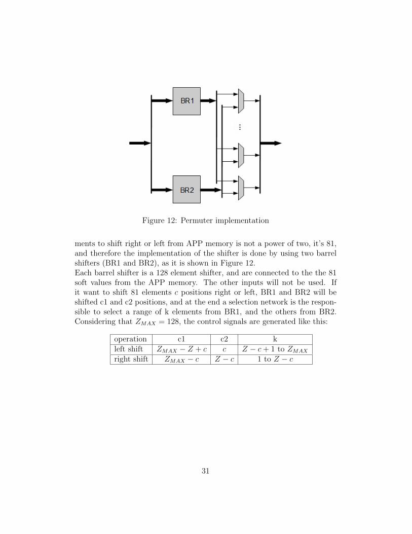
Figure 12: Permuter implementation

ments to shift right or left from APP memory is not a power of two, it’s 81,and therefore the implementation of the shifter is done by using two barrelshifters (BR1 and BR2), as it is shown in Figure 12.Each barrel shifter is a 128 element shifter, and are connected to the the 81soft values from the APP memory. The other inputs will not be used. Ifit want to shift 81 elements c positions right or left, BR1 and BR2 will beshifted c1 and c2 positions, and at the end a selection network is the respon-sible to select a range of k elements from BR1, and the others from BR2.Considering that ZMAX = 128, the control signals are generated like this:

operation c1 c2 kleft shift ZMAX − Z + c c Z − c+ 1 to ZMAX

right shift ZMAX − c Z − c 1 to Z − c

31

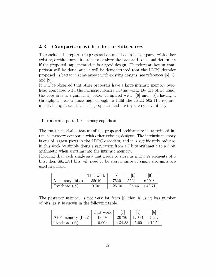
4.3 Comparison with other architectures

To conclude the report, the proposed decoder has to be compared with otherexisting architectures, in order to analyze the pros and cons, and determineif the proposed implementation is a good design. Therefore an honest com-parison will be done, and it will be demonstrated that the LDPC decoderproposed, is better in some aspect with existing designs, see references [6], [8]and [9].It will be observed that other proposals have a large intrinsic memory over-head compared with the intrinsic memory in this work. By the other hand,the core area is significantly lower compared with [6] and [8], having athroughput performance high enough to fulfil the IEEE 802.11n require-ments, being faster that other proposals and having a very low latency.

- Intrinsic and posterior memory coparison

The most remarkable feature of the proposed architecture is its reduced in-trinsic memory compared with other existing designs. The intrinsic memoryis one of largest parts in the LDPC decoders, and it is significantly reducedin this work by simply doing a saturation from a 7 bits arithmetic to a 5 bitarithmetic when writting into the intrinsic memory.Knowing that each single siso unit needs to store as much 88 elements of 5bits, then 88x5x81 bits will need to be stored, since 81 single siso units areused in parallel.

This work [8] [9] [6]λ-memory (bits) 35640 47520 55224 62208Overhead (%) 0.001 +25.00 +35.46 +42.71

The posterior memory is not very far from [9] that is using less numberof bits, as it is shown in the following table.

This work [8] [9] [6]APP memory (bits) 13608 20736 12960 15552Overhead (%) 0.001 +34.38 -5.00 +12.50

32

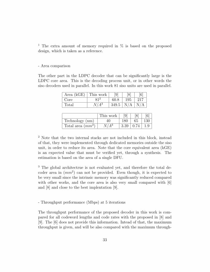
1 The extra amount of memory required in % is based on the proposeddesign, which is taken as a reference.

- Area comparison

The other part in the LDPC decoder that can be significantly large is theLDPC core area. This is the decoding process unit, or in other words thesiso decoders used in parallel. In this work 81 siso units are used in parallel.

Area (kGE) This work [9] [8] [6]Core 812 60.8 195 217Total N/A3 349.5 N/A N/A

This work [9] [8] [6]Technology (nm) 40 180 65 130Total area (mm2) N/A3 3.39 0.74 1.9

2 Note that the two internal stacks are not included in this block, insteadof that, they were implemented through dedicated memories outside the sisounit, in order to reduce its area. Note that the core equivalent area (kGE)is an expected value that must be verified yet, through a synthesis. Theestimation is based on the area of a single DFU.

3 The global architectrue is not evaluated yet, and therefore the total de-coder area in (mm2) can not be provided. Even though, it is expected tobe very small since the intrinsic memory was significantly reduced comparedwith other works, and the core area is also very small compared with [6]and [8] and close to the best implentation [9].

- Throughput performance (Mbps) at 5 iterations

The throughput performance of the proposed decoder in this work is com-pared for all codeword lengths and code rates with the proposed in [8] and[9]. The [6] does not provide this information. Intead of that, the maximumthroughput is given, and will be also compared with the maximum through-

33

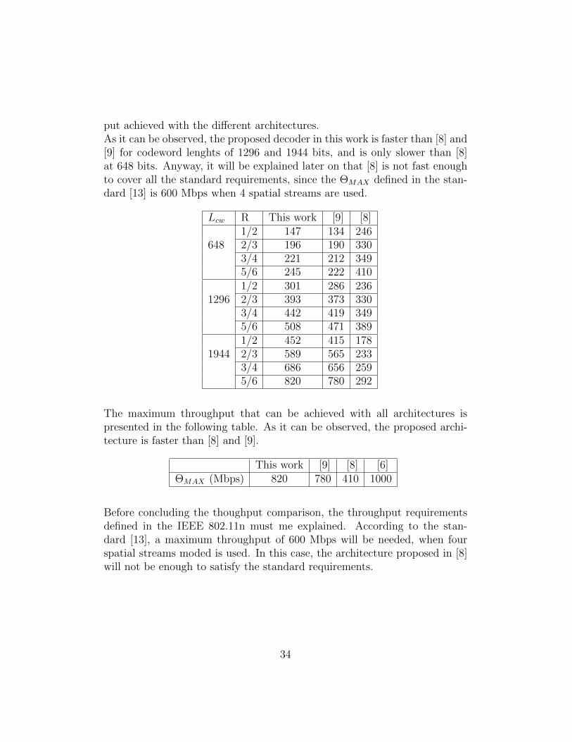
put achieved with the different architectures.As it can be observed, the proposed decoder in this work is faster than [8] and[9] for codeword lenghts of 1296 and 1944 bits, and is only slower than [8]at 648 bits. Anyway, it will be explained later on that [8] is not fast enoughto cover all the standard requirements, since the ΘMAX defined in the stan-dard [13] is 600 Mbps when 4 spatial streams are used.

Lcw R This work [9] [8]1/2 147 134 246

648 2/3 196 190 3303/4 221 212 3495/6 245 222 4101/2 301 286 236

1296 2/3 393 373 3303/4 442 419 3495/6 508 471 3891/2 452 415 178

1944 2/3 589 565 2333/4 686 656 2595/6 820 780 292

The maximum throughput that can be achieved with all architectures ispresented in the following table. As it can be observed, the proposed archi-tecture is faster than [8] and [9].

This work [9] [8] [6]ΘMAX (Mbps) 820 780 410 1000

Before concluding the thoughput comparison, the throughput requirementsdefined in the IEEE 802.11n must me explained. According to the stan-dard [13], a maximum throughput of 600 Mbps will be needed, when fourspatial streams moded is used. In this case, the architecture proposed in [8]will not be enough to satisfy the standard requirements.

34

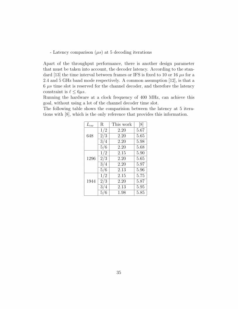
- Latency comparison (µs) at 5 decoding iterations

Apart of the throughput performance, there is another design parameterthat must be taken into account, the decoder latency. According to the stan-dard [13] the time interval between frames or IFS is fixed to 10 or 16 µs for a2.4 and 5 GHz band mode respectively. A common assumption [12], is that a6 µs time slot is reserved for the channel decoder, and therefore the latencyconstraint is ` ≤ 6µs.Running the hardware at a clock frequency of 400 MHz, can achieve thisgoal, without using a lot of the channel decoder time slot.The following table shows the comparision between the latency at 5 itera-tions with [8], which is the only reference that provides this information.

Lcw R This work [8]1/2 2.20 5.67

648 2/3 2.20 5.653/4 2.20 5.985/6 2.20 5.681/2 2.15 5.90

1296 2/3 2.20 5.653/4 2.20 5.975/6 2.13 5.961/2 2.15 5.75

1944 2/3 2.20 5.873/4 2.13 5.955/6 1.98 5.85

35

4.4 Conslusions

At this point, a detailed description of the decoder and its performance wasexposed. Additionally, it was compared with other existing architectures, interms of memory usage, core area, and latency.To sum up, the intrinsic memory saturation from a 7-bits arithmetic to a5-bit arithmetic, allows the decoder reduce significantly me intrinsic memorysize compared with the other architectures without an important distortion.This is probably the main merit of this work, because the intrinsic memoryis probably one of the biggest components in the decoder. This importantreduction compensates the stacks area. The core uses this stacks in order toreuse the architecture for any other kind of codes and standards.The core area is also another big part in the LDPC decoder, and the ap-proximation done was in a very compact and fast implementation. It wasshown that is not that far from [9], which is probably the most compactimplementation, but as it was said before the prposed architecture in thiswork is intended to be for multi-code and a multi-standard solution.To end this section, the the proposed architecture, is shown to be fast enoughto satisfy the sandard requirements, and also one of the fastest implementa-tions, only slower than [6].Therefore, all these aspects conrtribute to a compact, fast and the possibil-ity to extend it to other codes and standards. Looking at the results, theproposed architecture is not the best in terms of thoughput, and area, butin all cases its performance is very close to the best one. The best proposaltaking into account all aspects is [6], which offers a very good throughputperfomance and a very small core area.By the other hand [8] and [9] have a very large core area, but even thatthroughput can be higher, is more important to provide a throughput thatcan satisfy the standard requirements, and try to reduce the area instead offocus the design in provide a massive throughput.For all these reasons, it can be concluded that the architectures proposed inthis work can be considered a very good solution.

4.5 Future work

The full architecture has to be evaluated yet, that means that the memories,the permuter, the decoder core and the control unit have to be connected,and parameters such as the total area and the power consumption must be

36

analyzed, even though the area is spected to be small.In addition, once the full architecture is completed, the next step add theextra part to make the solution reusable for other codes and standards. TheSISO unit, was designed taking into account this. In [7], a turbo-LDPC de-coder architecture is introduced, which uses the same structure, so to extendthe proposed architecture in this work, this is a good point to get started.

37

References

[1] Muhammad M. Mansour and Naresh R. Shanbhag, “High-ThroughputLDPC Decoders”, IEEE Transactions on very large scale integrationsystems, vol. 11, no. 6, pp. 976-996, Dec. 2003.

[2] Muhammad M. Mansour and Naresh R. Shanbhag, “A 640-Mbs 2048-Bit Programmable LDPC Decoder Chip”, IEEE Journal of solid-statecircuits, vol. 41, no. 3, pp. 684-697, March 2006.

[3] Muhammad M. Mansour, “A Turbo-Decoding Message-Passing Algo-rithm for Sparse Parity-Check Matrix Codes”, IEEE Transactions onsignal processing, vol. 54, no. 11, pp. 4376-4392, Nov. 2006.

[4] Yang Sun, Marjan Karkooti and Joseph Caballaro, “High throughput,parallel scalable LDPC encoder/decoder architecture for OFDM sys-tems”, IEEE Dallas/CAS Workshop on design, applications, integrationand software, pp. 39-42, Oct. 2006.

[5] Yang Sun and Joseph Caballaro, “A low-power 1-Gbps reconfigurableLDPC decoder design for multiple 4G wireless standards”, IEEE SOCconference, pp. 4376-4392, Sep. 2008.

[6] Yang Sun, Marjan Karkooti and Joseph Caballaro, “VLSI DecoderArchitecture for High Throughput, Variable Block-size and Multi-rateLDPC Codes”, IEEE International Symposium on Circuits and Systems,pp. 2104-2107, May. 2007.

[7] Yang Sun and Joseph Caballaro, “A Flexible LDPC/Turbo DecoderArchitecture”, Springer Journal of Signal Processing Systems, vol. 64,no. 1, pp. 1-16, 2011.

[8] Massimo Rovini, Giuseppe Gentile, Francesco Rossi and Luca Fanucci,“A Scalable Decoder Architecture for IEEE 802.11n LDPC Codes”,IEEE GLOBECOM, pp. 3270-3274, Nov. 2007.

[9] C. Studer, N. Preyss, C. Roth and A. Burg, “Configurable High-Throughput Decoder Architecture for Quasi-Cyclic LDPC Codes”,IEEE Conference on signals, systems and computers, pp. 1137-1142,Oct. 2008.

38

[10] Xiao-Yu Hu, Evangelos Eleftheriou, Dieter-Michael Arnold and AjayDholakia, “Efficient implementations of the SPA for decoding LDPCCodes”, IBM Research, Zurich Research Laboratory / IEEE GLOBE-COM, vol. 2, pp. 1036-1036E, 2001.

[11] Joachim Hagenauer, “The Turbo Principle - Tutorial introduction andstate of the art”, International Symposium on Turbo Codes (Brest,France) / Technical University of Munich, 1997.

[12] Raffaele Riva, “LDPC codes for W-LAN IEEE 802.11n: an overview”,LDPC@work (Pisa, Italy) / ST, 6th October 2006.

[13] IEEE 802.11n, IEEE Standard for Information technology - Part 11:Wireless LAN Medium Acces Control (MAC) and Physical Layer (PHY)Specifications. Amendment 5: Enhancements for Higher Throughput,29th Oct. 2009.

[14] Bernard Sklar, Digital Communications. Fundamentals and applications,Prentice Hall (2nd edition).

[15] Jorge Castineira Moreira and Patrick Guy Farrel, Essentials of error-control coding, John Wiley and sons (2006).

[16] David J. C. MacKay, Information Theory, Inference and Learning Al-gorithms, Cambridge University Press (2003).

[17] David J. C. MacKay’s website, www.inference.phy.cam.ac.uk.mackay.

[18] IT++ libraries, itpp.sourceforge.net/current/index.html.

39

A Throughput specifications

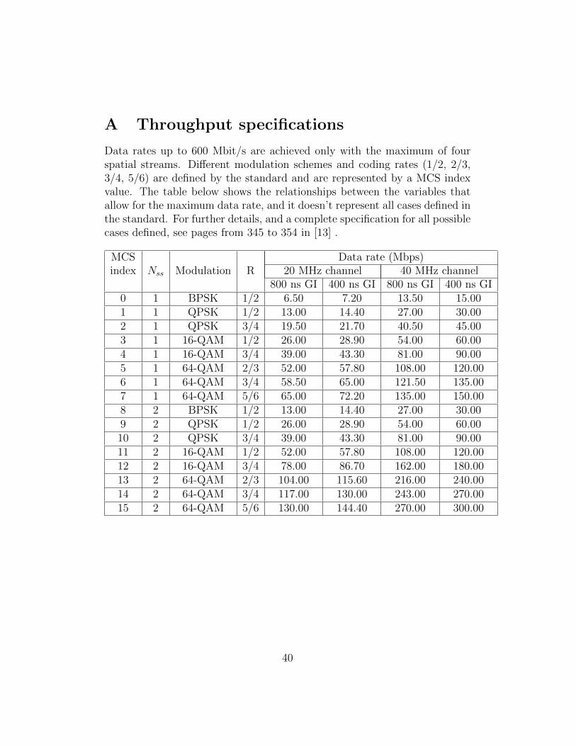
Data rates up to 600 Mbit/s are achieved only with the maximum of fourspatial streams. Different modulation schemes and coding rates (1/2, 2/3,3/4, 5/6) are defined by the standard and are represented by a MCS indexvalue. The table below shows the relationships between the variables thatallow for the maximum data rate, and it doesn’t represent all cases defined inthe standard. For further details, and a complete specification for all possiblecases defined, see pages from 345 to 354 in [13] .

MCS Data rate (Mbps)index Nss Modulation R 20 MHz channel 40 MHz channel

800 ns GI 400 ns GI 800 ns GI 400 ns GI0 1 BPSK 1/2 6.50 7.20 13.50 15.001 1 QPSK 1/2 13.00 14.40 27.00 30.002 1 QPSK 3/4 19.50 21.70 40.50 45.003 1 16-QAM 1/2 26.00 28.90 54.00 60.004 1 16-QAM 3/4 39.00 43.30 81.00 90.005 1 64-QAM 2/3 52.00 57.80 108.00 120.006 1 64-QAM 3/4 58.50 65.00 121.50 135.007 1 64-QAM 5/6 65.00 72.20 135.00 150.008 2 BPSK 1/2 13.00 14.40 27.00 30.009 2 QPSK 1/2 26.00 28.90 54.00 60.0010 2 QPSK 3/4 39.00 43.30 81.00 90.0011 2 16-QAM 1/2 52.00 57.80 108.00 120.0012 2 16-QAM 3/4 78.00 86.70 162.00 180.0013 2 64-QAM 2/3 104.00 115.60 216.00 240.0014 2 64-QAM 3/4 117.00 130.00 243.00 270.0015 2 64-QAM 5/6 130.00 144.40 270.00 300.00

40

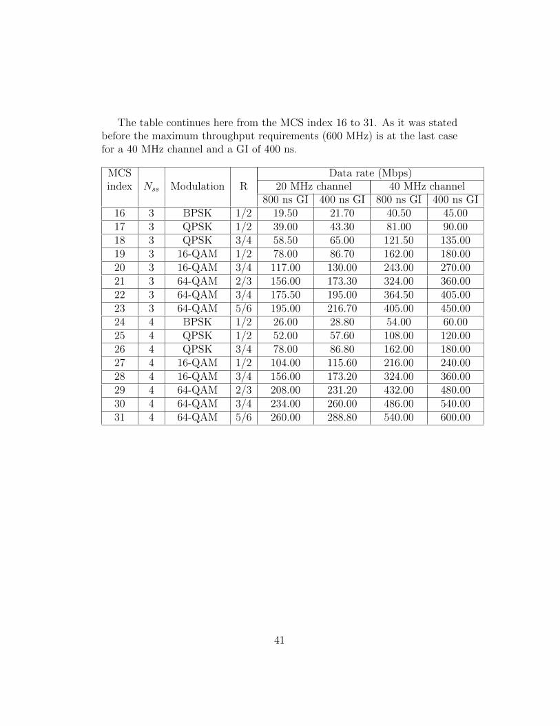
The table continues here from the MCS index 16 to 31. As it was statedbefore the maximum throughput requirements (600 MHz) is at the last casefor a 40 MHz channel and a GI of 400 ns.

MCS Data rate (Mbps)index Nss Modulation R 20 MHz channel 40 MHz channel

800 ns GI 400 ns GI 800 ns GI 400 ns GI16 3 BPSK 1/2 19.50 21.70 40.50 45.0017 3 QPSK 1/2 39.00 43.30 81.00 90.0018 3 QPSK 3/4 58.50 65.00 121.50 135.0019 3 16-QAM 1/2 78.00 86.70 162.00 180.0020 3 16-QAM 3/4 117.00 130.00 243.00 270.0021 3 64-QAM 2/3 156.00 173.30 324.00 360.0022 3 64-QAM 3/4 175.50 195.00 364.50 405.0023 3 64-QAM 5/6 195.00 216.70 405.00 450.0024 4 BPSK 1/2 26.00 28.80 54.00 60.0025 4 QPSK 1/2 52.00 57.60 108.00 120.0026 4 QPSK 3/4 78.00 86.80 162.00 180.0027 4 16-QAM 1/2 104.00 115.60 216.00 240.0028 4 16-QAM 3/4 156.00 173.20 324.00 360.0029 4 64-QAM 2/3 208.00 231.20 432.00 480.0030 4 64-QAM 3/4 234.00 260.00 486.00 540.0031 4 64-QAM 5/6 260.00 288.80 540.00 600.00

41

B Parity-check matrices definitions

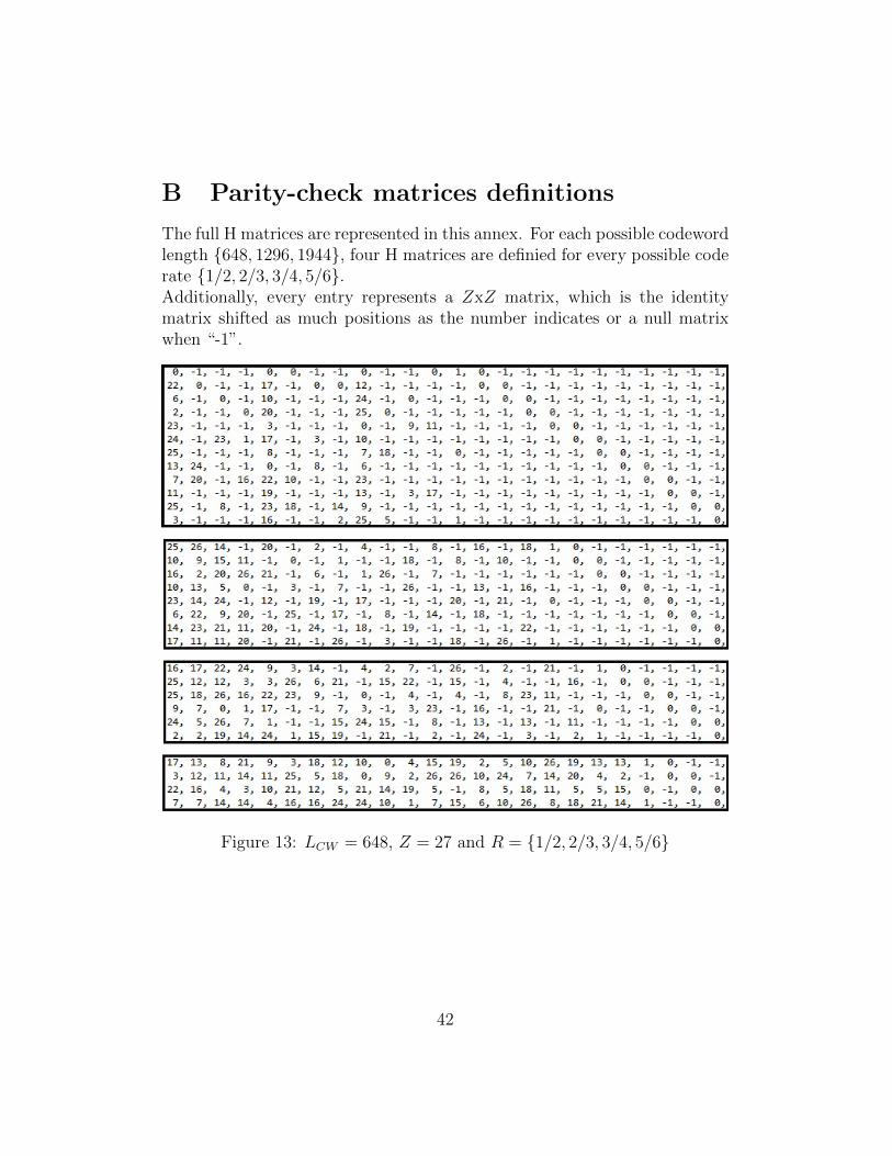
The full H matrices are represented in this annex. For each possible codewordlength {648, 1296, 1944}, four H matrices are definied for every possible coderate {1/2, 2/3, 3/4, 5/6}.Additionally, every entry represents a ZxZ matrix, which is the identitymatrix shifted as much positions as the number indicates or a null matrixwhen “-1”.

Figure 13: LCW = 648, Z = 27 and R = {1/2, 2/3, 3/4, 5/6}

42

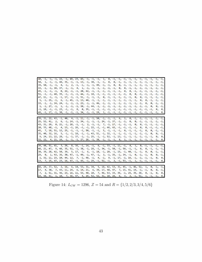
Figure 14: LCW = 1296, Z = 54 and R = {1/2, 2/3, 3/4, 5/6}

43

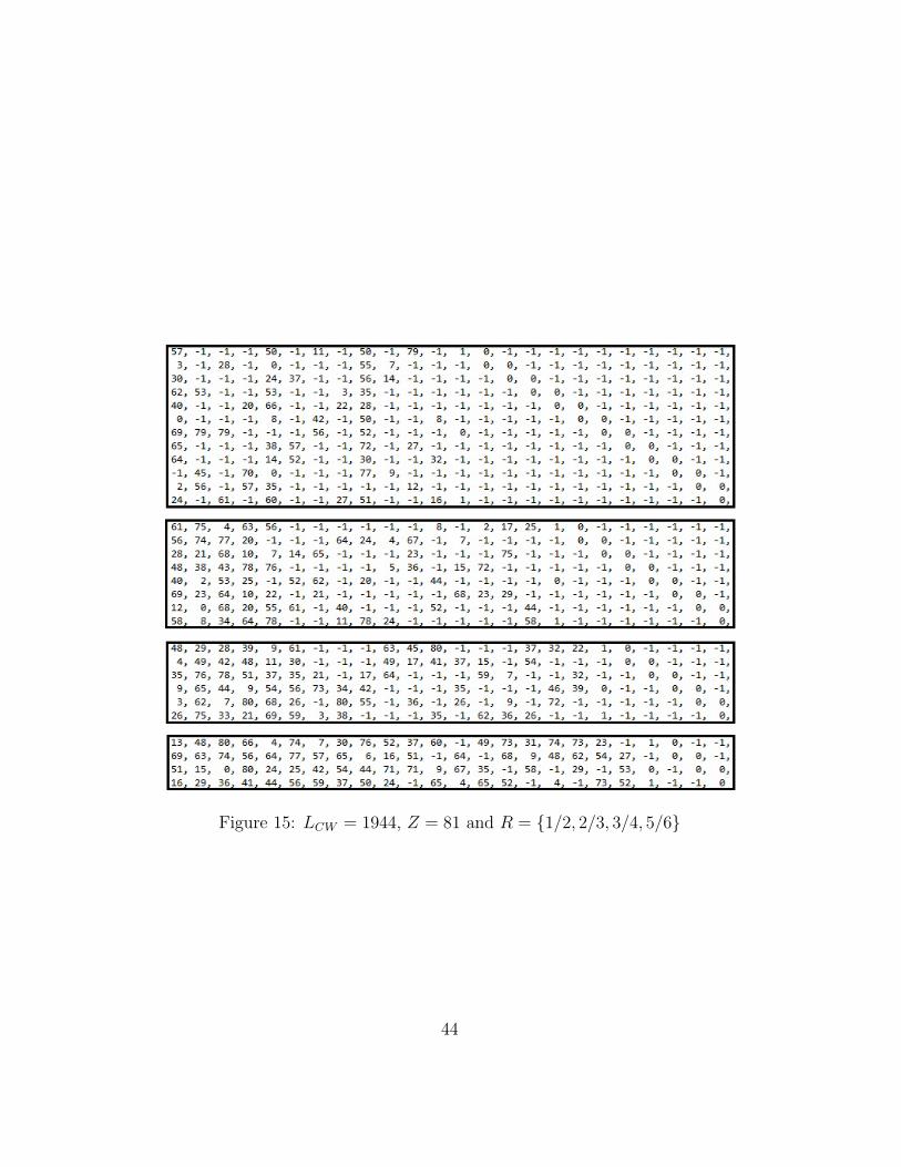
Figure 15: LCW = 1944, Z = 81 and R = {1/2, 2/3, 3/4, 5/6}

44