Embed Size (px)
Citation preview
DESIGN METHODOLOGIES FOR
INSTRUCTION-SET EXTENSIBLE
PROCESSORS
YU, PAN
NATIONAL UNIVERSITY OF SINGAPORE
2008
Design Methodologies for Instruction-Set
Extensible Processors
Yu, Pan
(B.Sci., Fudan University)
A thesis submitted for the degree of Doctor of Philosophy
in Computer Science
Department of Computer Science
National University of Singapore
2008

List of Publications
Y. Pan, and T. Mitra, Characterizing embedded applications for instruction-set
extensible processors, In the Proceedings of Design Automation Conference (DAC),
2004.
Y. Pan, and T. Mitra. Scalable custom instructions identification for instruction-set
extensible processors. In the Proceedings of International Conference on Compilers,
Architectures, and Synthesis for Embedded Systems (CASES), 2005.
Y. Pan and T. Mitra. Satisfying real-time constraints with custom instructions. In
the Proceedings of International Conference on Hardware/Software Codesign and
System Synthesis (CODES+ISSS), 2005.
Y. Pan and T. Mitra. Disjoint pattern enumeration for custom instructions iden-
tification. In the Proceedings of International Conference on Field Programmable
Logic and applications (FPL), 2007.
Acknowledgement
I would like to thank my advisor professor Tulika Mitra for her guidance. Her
broad knowledge and working style as a scientist, care and patience as a teacher
have always been the example for me. I feel very fortunate to be her student. I
wish to thank the members of my thesis committee, professor Wong Weng Fai,
professor Samarjit Chakraborty and professor Laura Pozzi for their discussions and
encouraging comments during the early stage of this work. This thesis would not
have been possible without their support.
I would like to thank my fellow colleagues in the embedded system lab. They
are, Kathy Nguyen Dang, Phan Thi Xuan Linh, Ge Zhiguo, Edward Sim Joon, Zhu
Yongxin, Li Xianfeng, Liao Jirong, Liu Haibin, Hemendra Singh Negi, Hariharan
Sandanagobalane, Ramkumar Jayaseelan, Unmesh Dutta Bordoloi, Liang Yun, and
Huynh Phung Huynh. The common interests shared among the brothers and sisters
of this big family have been my constant source of inspiration. My best friends Zhou
Zhi, Wang Huiqing, Miao Xiaoping, Ni Wei and Ge Hong have given me tremendous
strength and back up all along. And most importantly, thanks to Yang Xiaoyan,
my fiancee, for her accompany and endurance during all these years.
My parents and my grand parents, they raised, inspired me, and always stand
by me no matter what. My love and gratitude to them is beyond words. I wish my
grand parents in heaven would be proud of my achievements, and to hug my parents
tightly in my arms — at home.
ii

Contents
List of Publications i
Acknowledgement ii
Contents iii
Abstract ix
List of Figures x
List of Tables xv
1 Introduction 1
1.1 Specialization . . . . . . . . . . . . . . . . . . . . . . . . . . . . . . . 2
1.1.1 Inefficiency of General Purpose Processors . . . . . . . . . . . 3
1.1.2 ASICs — the Extreme Specialization . . . . . . . . . . . . . . 5
1.1.3 Software vs. Hardware . . . . . . . . . . . . . . . . . . . . . . 6
iii

CONTENTS iv
1.1.4 Spectrum of Specializations . . . . . . . . . . . . . . . . . . . 6
1.1.5 FPGAs and Reconfigurable Computing . . . . . . . . . . . . . 11
1.2 Instruction-set Extensible Processors . . . . . . . . . . . . . . . . . . 14
1.2.1 Hardware-Software Partitioning . . . . . . . . . . . . . . . . . 16
1.2.2 Compiler and Intermediate Representation . . . . . . . . . . . 18
1.2.3 An Overview of the Design Flow . . . . . . . . . . . . . . . . 19
1.3 Contributions and Organization of this Thesis . . . . . . . . . . . . . 20
2 Instruction-Set Extensible Processors 24
2.1 Past Systems . . . . . . . . . . . . . . . . . . . . . . . . . . . . . . . 24
2.1.1 DISC . . . . . . . . . . . . . . . . . . . . . . . . . . . . . . . . 25
2.1.2 Garp . . . . . . . . . . . . . . . . . . . . . . . . . . . . . . . . 26
2.1.3 PRISC . . . . . . . . . . . . . . . . . . . . . . . . . . . . . . . 28
2.1.4 Chimaera . . . . . . . . . . . . . . . . . . . . . . . . . . . . . 30
2.1.5 CCA . . . . . . . . . . . . . . . . . . . . . . . . . . . . . . . . 31
2.1.6 PEAS . . . . . . . . . . . . . . . . . . . . . . . . . . . . . . . 33
2.1.7 Xtensa . . . . . . . . . . . . . . . . . . . . . . . . . . . . . . . 34
2.2 Design Issues and Options . . . . . . . . . . . . . . . . . . . . . . . . 36
2.2.1 Instruction Encoding . . . . . . . . . . . . . . . . . . . . . . . 36
2.2.2 Crossing the Control Flow . . . . . . . . . . . . . . . . . . . . 38

CONTENTS v
3 Related Works 41
3.1 Candidate Pattern Enumeration . . . . . . . . . . . . . . . . . . . . . 42
3.1.1 A Classification of Previous Custom Instruction Enumeration
Methods . . . . . . . . . . . . . . . . . . . . . . . . . . . . . . 43
3.2 Custom Instruction Selection . . . . . . . . . . . . . . . . . . . . . . 46
4 Scalable Custom Instructions Identification 50
4.1 Custom Instruction Enumeration Problem . . . . . . . . . . . . . . . 51
4.1.1 Problem Definition . . . . . . . . . . . . . . . . . . . . . . . . 52
4.2 Exhaustive Pattern Enumeration . . . . . . . . . . . . . . . . . . . . 56
4.2.1 SingleStep Algorithm . . . . . . . . . . . . . . . . . . . . . . . 56
4.2.2 MultiStep Algorithm . . . . . . . . . . . . . . . . . . . . . . . 57
4.2.3 Generation of Cones . . . . . . . . . . . . . . . . . . . . . . . 59
4.2.4 Generation of Connected MIMO Patterns . . . . . . . . . . . 61
4.2.5 Generation of Disjoint MIMO Patterns . . . . . . . . . . . . . 69
4.2.6 Optimizations . . . . . . . . . . . . . . . . . . . . . . . . . . . 73
4.3 Experimental Results . . . . . . . . . . . . . . . . . . . . . . . . . . . 79
4.3.1 Experimental Setup . . . . . . . . . . . . . . . . . . . . . . . . 79
4.3.2 Comparison on Connected Pattern Enumeration . . . . . . . . 80
CONTENTS vi
4.3.3 Comparison on All Feasible Pattern Enumeration . . . . . . . 82
4.4 Summary . . . . . . . . . . . . . . . . . . . . . . . . . . . . . . . . . 85
5 Custom Instruction Selection 87
5.1 Custom Instruction Selection . . . . . . . . . . . . . . . . . . . . . . 88
5.1.1 Optimal Custom Instruction Selection using ILP . . . . . . . . 88
5.1.2 Experiments on the Effects of Custom Instructions . . . . . . 90
5.2 A Study on the Potential of Custom Instructions . . . . . . . . . . . 94
5.2.1 Crossing the Basic Block Boundaries . . . . . . . . . . . . . . 95
5.2.2 Experimental Setup . . . . . . . . . . . . . . . . . . . . . . . . 98
5.2.3 Results and Analysis . . . . . . . . . . . . . . . . . . . . . . . 100
5.3 Summary . . . . . . . . . . . . . . . . . . . . . . . . . . . . . . . . . 107
6 Improving WCET with Custom Instructions 108
6.1 Motivation . . . . . . . . . . . . . . . . . . . . . . . . . . . . . . . . . 109
6.1.1 Related Work to Improve WCET . . . . . . . . . . . . . . . . 110
6.2 Problem Formulation . . . . . . . . . . . . . . . . . . . . . . . . . . . 111
6.2.1 WCET Analysis using Timing Schema . . . . . . . . . . . . . 112
6.3 Optimal Solution Using ILP . . . . . . . . . . . . . . . . . . . . . . . 113

CONTENTS vii
6.4 Heuristic Algorithm . . . . . . . . . . . . . . . . . . . . . . . . . . . . 116
6.4.1 Computing Profits for Patterns . . . . . . . . . . . . . . . . . 117
6.4.2 Improving the Heuristic . . . . . . . . . . . . . . . . . . . . . 119
6.5 Experimental Evaluation . . . . . . . . . . . . . . . . . . . . . . . . . 122
6.6 Summary . . . . . . . . . . . . . . . . . . . . . . . . . . . . . . . . . 126
7 Conclusions 127
A ISE Tool on Trimaran 141
A.1 Work Flow . . . . . . . . . . . . . . . . . . . . . . . . . . . . . . . . . 142
A.2 Limitations of the Tool . . . . . . . . . . . . . . . . . . . . . . . . . . 144

Abstract
The machine unmakes the man. Now that the machine is so perfect, the
engineer is nobody. – Ralph Waldo Emerson
Customizing the processor core, by extending its instruction set architecture
with application specific custom instructions, is becoming more and more popular
to meet the increasing performance requirement of embedded system design. The
proliferation of high performance reprogrammable hardware makes this approach
even more flexible. By integrating custom functional units (CFU) in parallel with
standard ALUs in the processor core, the processor can be configured to accelerate
different applications. A single custom instruction encapsulates a frequently occur-
ring computation pattern involving multiple primitive operations. Parallelism and
logic optimization among these operations can be exploited to implement the CFU,
which leads to improved performance over executing the operations individually in
basic function units. Other benefits of using custom instructions, such as compact
code size, reduced register pressure, and less memory hierarchy overhead, contribute
to improved energy efficiency.
The fundamental problem of the instruction-set extensible processor design is
the hardware-software partitioning problem, which identifies the set of custom in-
structions for a given application. Custom instructions are identified on the dataflow
graph of the application. This problem can be further divided into two subproblems:
viii

ABSTRACT ix
(1) enumeration of the set of feasible subgraphs (patterns) of the dataflow graph as
candidates custom instructions, and (2) choosing a subset of these subgraphs to
cover the application for optimized performance under various design constraints.
However, solving both subproblems optimally are intractable and computationally
expensive. Most previous works impose strong restrictions on the topology of pat-
terns to reduce the number of candidates, and then use heuristics to choose a suitable
subset.
Through our study, we find that the number of all the possible candidate pat-
terns under relaxed architectural constraints is far from exponential. However, the
current state-of-the-art enumeration algorithms do not scale well when the size of
dataflow graph increases. These large dataflow graphs pack considerable execution
parallelism and are ideal to make use of custom instructions. Moreover, modern
compiler transformations also form large dataflow graphs across the control flow to
expose more parallelism. Therefore, scalable and high quality custom instruction
identification methodologies are required.
The contributions of this thesis are the following. First, we propose efficient
and scalable subgraph enumeration algorithms for candidate custom instructions.
Through exhaustive enumeration, isomorphic subgraphs embedded inside the dataflow
graphs, which can be covered by the same custom instruction, are fully exposed.
Second, based on our custom instruction identification methodology, we conduct a
systematic study of the effects and correlations between various design constraints
and system performance on a broad range of embedded applications. This study
provides a valuable reference for the design of general extensible processors. Finally,
we apply our methodologies in the context of real-time systems, to improve the
worst-case execution time of applications using custom instructions.

List of Figures
1.1 Performance overhead of using general purpose instructions, for a bit
permutation example in DES encryption algorithm (adapted from [44]). 3
1.2 Architecture of a 16-bit, 3-input adder (adapted from [32]). . . . . . . 5
1.3 Spectrum of system specialization. . . . . . . . . . . . . . . . . . . . 8
1.4 MAC in a DSP. (a) Chaining basic operations on the dataflow, (b)
Block diagram of a MAC unit. . . . . . . . . . . . . . . . . . . . . . . 9
1.5 General structure of a FPGA. . . . . . . . . . . . . . . . . . . . . . . 11
1.6 Typical LUT based logic block. (a) A widely used 4-input 1-output
LUT, (b) Block diagram of the logic block. . . . . . . . . . . . . . . . 13
1.7 General architecture of instruction-set extensible processors. (a) Cus-
tom functional units (CFU) embedded in the processor datapath, (b)
A complex computation pattern encapsulated as a custom instruction. 15
1.8 Intermediate representation. (a) Source code of a function (adapted
from Secure Hash Algorithm), (b) Its control flow graph, (c) Dataflow
graph of basic block 1. . . . . . . . . . . . . . . . . . . . . . . . . . . 19
x
LIST OF FIGURES xi
1.9 Compile time instruction-set extension design flow. . . . . . . . . . . 21
2.1 DISC system (adapted from [81]). . . . . . . . . . . . . . . . . . . . . 25
2.2 PRISC system (adapted from [70]). (a) Datapath, (b) Format of the
32-bit FPU instruction. . . . . . . . . . . . . . . . . . . . . . . . . . . 28
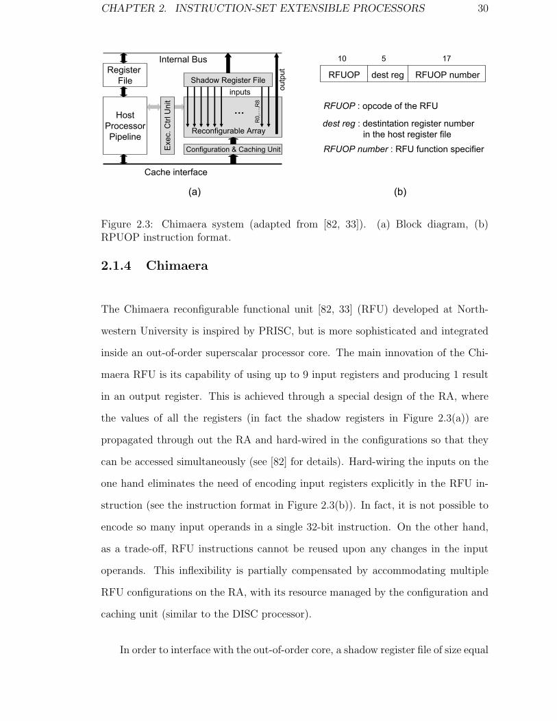
2.3 Chimaera system (adapted from [82, 33]). (a) Block diagram, (b)
RPUOP instruction format. . . . . . . . . . . . . . . . . . . . . . . . 30
2.4 The CCA system (adapted from [21, 20]). (a) The CCA (Configurable
Compute Accelerator), (b) System architecture. . . . . . . . . . . . . 31
2.5 The PEAS environment (adapted from [71, 46]). (a) Main functions
of the system, (b) Micro-operation description of the ADDU instruction. 33
2.6 Ways of forming custom instructions across the control flow. (a)
Downward code motion, (b) Predicated execution, (c) Control local-
ization. . . . . . . . . . . . . . . . . . . . . . . . . . . . . . . . . . . . 38
3.1 Dataflow graph. (a) Two non-overlapped candidate patterns, (b)
Overlapped candidate patterns, (c) Overlapped patterns cannot be
scheduled together. . . . . . . . . . . . . . . . . . . . . . . . . . . . . 43
4.1 An example dataflow graph. Valid nodes are numbered according
to reverse topological order. Invalid nodes corresponding to memory
load operations (LD) are unshaded. Two regions are separated by a
LD operation. . . . . . . . . . . . . . . . . . . . . . . . . . . . . . . . 52

LIST OF FIGURES xii
4.2 Forming a feasible connected MIMO pattern through partial decom-
position. Decomposition cones are dashed on each step. Trivial de-
composition cones, like {1} for every downward extension and {2} in
pd3, are omitted. They are eliminated in the algorithm. . . . . . . . . 62
4.3 Generating all feasible connected patterns involving node 1. . . . . . 64
4.4 A recursive process of collecting patterns for the example in Fig. 4.3. 64
4.5 Non-connectivity/Convexity check based on upward scope. (a) p2
connects with p1. (b) p2 introduces non-convexity. . . . . . . . . . . 71
4.6 Bypass pointers (dashed arrows) on a linked list of patterns. . . . . . 78
4.7 Run time speedup (MultiStep/SingleStep) for connected patterns. . . 82
4.8 Run time speedup (MultiStep/SingleStep) for all feasible patterns. . . 84
5.1 Subgraph convexity. (a) A non-convex subgraph, (b) Two interde-
pendent convex subgraphs, (c) The left subgraph turns non-convex
after the right one is reduced to a custom instruction; consequently
the left subgraph cannot be selected. . . . . . . . . . . . . . . . . . . 89
5.2 Potential effect of custom instructions. . . . . . . . . . . . . . . . . . 92
5.3 Effect of custom instructions. . . . . . . . . . . . . . . . . . . . . . . 93
5.4 Possible correlations of branches. (a) Left (right) side of the 1st
branch is always followed by the left (right) side of the 2nd one,
(b) Left (right) side of the 1st branch is always followed by the right
(left) side of the 2nd one. . . . . . . . . . . . . . . . . . . . . . . . . . 96
LIST OF FIGURES xiii
5.5 WPP for basic block sequence 0134601346013460134602356023567
with execution count annotations. . . . . . . . . . . . . . . . . . . . . 97
5.6 Comparison of MISO and MIMO. . . . . . . . . . . . . . . . . . . . . 101
5.7 Effect of Number of Input Operands. . . . . . . . . . . . . . . . . . . 102
5.8 Effect of area constraint. . . . . . . . . . . . . . . . . . . . . . . . . . 103
5.9 Effect of constraint on total number of custom instructions. . . . . . . 103
5.10 Effect of relaxing control flow constraints. . . . . . . . . . . . . . . . 104
5.11 Reduction across basic blocks under varying area budgets. . . . . . . 105
5.12 Effect of number of input operands under 3 outputs across basic blocks.105
5.13 Contributions of cycle count reduction due to custom instructions
across loop or if branches. . . . . . . . . . . . . . . . . . . . . . . . . 106
6.1 An motivating example. . . . . . . . . . . . . . . . . . . . . . . . . . 109
6.2 CFG and syntax tree corresponding to the code in Figure 6.1 . . . . . 112
6.3 Efficient computation of profit function. . . . . . . . . . . . . . . . . . 118
6.4 Limitation of the heuristic. . . . . . . . . . . . . . . . . . . . . . . . . 120
A.1 Pattern {1, 3} cannot be used without resolving WAR dependency
between node 2 and 3 (caused by reusing register R3). . . . . . . . . . 142
A.2 Work flow of ISE enabled compilation. . . . . . . . . . . . . . . . . . 143

LIST OF FIGURES xiv
A.3 Order of custom instruction insertion. (a) Original operations is topo-
logically ordered correctly (adapted from [22]), (b) The partial order
is broken (node 4 and 3) after custom instruction replacement. . . . 144
List of Tables
1.1 Software vs. Hardware. . . . . . . . . . . . . . . . . . . . . . . . . . . 7
1.2 GPP vs. ASIC . . . . . . . . . . . . . . . . . . . . . . . . . . . . . . 7
4.1 Benchmark characteristics. The size of basic block and region are
given in terms of number of nodes (instructions). . . . . . . . . . . . 80
4.2 Comparison of enumeration algorithms – connected patterns . . . . . 81
4.3 Comparison of enumeration algorithms – disjoint patterns . . . . . . 83
5.1 Benchmark characteristics. . . . . . . . . . . . . . . . . . . . . . . . . 91
5.2 Characteristics of benchmark programs . . . . . . . . . . . . . . . . . 99
6.1 Benchmark Characteristics. . . . . . . . . . . . . . . . . . . . . . . . 122
6.2 WCET Reduction under 5 custom instruction constraint with con-
strained topology. . . . . . . . . . . . . . . . . . . . . . . . . . . . . . 124
6.3 WCET Reduction under 5 custom instruction constraint with relaxed
topology. . . . . . . . . . . . . . . . . . . . . . . . . . . . . . . . . . . 124
xv

LIST OF TABLES xvi
6.4 WCET Reduction under resource constraint of 20 32-bit full adders
with relaxed topology. . . . . . . . . . . . . . . . . . . . . . . . . . . 125
6.5 WCET Reduction under 10 custom instruction constraint with re-
laxed topology. . . . . . . . . . . . . . . . . . . . . . . . . . . . . . . 125

Chapter 1
Introduction
The breeding of distantly related or unrelated individuals often produces
a hybrid of superior quality. – The American Heritage Dictionary, in the
paraphrase of “outbreeding”.
Driven by the advances of semiconductor industry during the past three decades,
electronic products with computation capability have permeated into every aspect of
our daily work and life. Such devices like industrial machines, household appliances,
medical equipments, automobiles, or recently popular cell phones, MP3 player and
digital cameras, are very different from general purpose computer systems such as
workstations and PCs in both appearance and functions. As their cores of compu-
tation are usually small and hidden behind the scenes, they are called Embedded
Systems. In fact, there are far more embedded applications than those using gen-
eral purpose computers. There is research showing that everyone among the urban
population is surrounded by more than 10 embedded devices.
Though there is no standard definition for embedded systems, the most impor-
tant characteristic is included in a general one: an Embedded System is any computer
system or computing device that performs a dedicated function or is designed for
1

CHAPTER 1. INTRODUCTION 2
use with a specific embedded software application. Most embedded computers
run the same application during their entire lifetime, and such applications usually
have relatively small and well-defined computation kernels and more regular data
sets than general-purpose applications [69]. The additional knowledge of the deter-
minacy, on the one hand, offers more opportunities to explore system effectiveness;
on the other hand, it raises the design challenges in that the hardware architecture
should be specialized to best suit the given application.
1.1 Specialization
An effective embedded system for a given application is always designed around var-
ious constraints. A product should not only meet its computational requirements,
i.e., the performance constraints, but also needs to be cost effective and efficient,
in terms of silicon area and power consumption constraints. A general purpose
computer for a simple task like operating a washing machine is overkill and very
expensive. On the other hand, the same general purpose computer may be ineffi-
cient or even infeasible for certain I/O, data or computational intensive applications
requiring very high throughput, such as network processing, image processing, en-
cryption among others. Power consumption is frequently a major concern of many
portable devices, which renders power hungry general purpose computers less favor-
able. For real-time embedded systems, timing constraints must be assured for task
executions to meet their deadlines. Ideally, an embedded system should provide suf-
ficient performance at minimum cost and power consumption. One way to achieve
this is specialization — the exploitation and translation of application peculiarities
into the system design. Specialization involves many aspects such as the design of
processing unit, memory system, interconnecting network topology and others. This
thesis focuses on the processing unit design — the heart of the computation.
CHAPTER 1. INTRODUCTION 3
srl $13, $2, 20andi $25, $13, 1srl $14, $2, 21andi $24, $14, 6or $15, $25, $24srl $13, $2, 22andi $14, $13, 56or $25, $15, $14sll $24, $25, 2
Sequence of MIPS instructions
27 26 25 23 22 20
7 6 5 4 3 20. . . 0 . . .
Actual bit-level logic (wiring only)
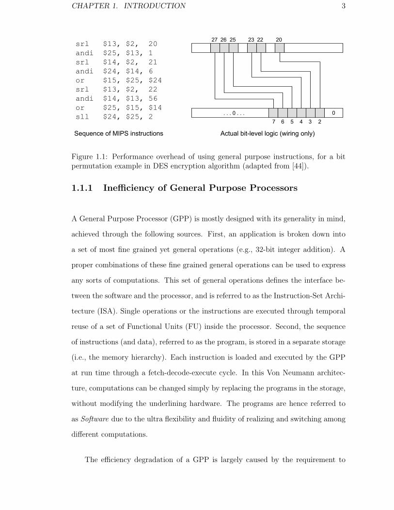
Figure 1.1: Performance overhead of using general purpose instructions, for a bitpermutation example in DES encryption algorithm (adapted from [44]).
1.1.1 Inefficiency of General Purpose Processors
A General Purpose Processor (GPP) is mostly designed with its generality in mind,
achieved through the following sources. First, an application is broken down into
a set of most fine grained yet general operations (e.g., 32-bit integer addition). A
proper combinations of these fine grained general operations can be used to express
any sorts of computations. This set of general operations defines the interface be-
tween the software and the processor, and is referred to as the Instruction-Set Archi-
tecture (ISA). Single operations or the instructions are executed through temporal
reuse of a set of Functional Units (FU) inside the processor. Second, the sequence
of instructions (and data), referred to as the program, is stored in a separate storage
(i.e., the memory hierarchy). Each instruction is loaded and executed by the GPP
at run time through a fetch-decode-execute cycle. In this Von Neumann architec-
ture, computations can be changed simply by replacing the programs in the storage,
without modifying the underlining hardware. The programs are hence referred to
as Software due to the ultra flexibility and fluidity of realizing and switching among
different computations.
The efficiency degradation of a GPP is largely caused by the requirement to
CHAPTER 1. INTRODUCTION 4
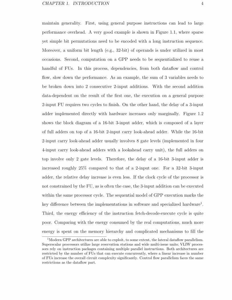
maintain generality. First, using general purpose instructions can lead to large
performance overhead. A very good example is shown in Figure 1.1, where sparse
yet simple bit permutations need to be encoded with a long instruction sequence.
Moreover, a uniform bit length (e.g., 32-bit) of operands is under utilized in most
occasions. Second, computation on a GPP needs to be sequentialized to reuse a
handful of FUs. In this process, dependencies, from both dataflow and control
flow, slow down the performance. As an example, the sum of 3 variables needs to
be broken down into 2 consecutive 2-input additions. With the second addition
data-dependent on the result of the first one, the execution on a general purpose
2-input FU requires two cycles to finish. On the other hand, the delay of a 3-input
adder implemented directly with hardware increases only marginally. Figure 1.2
shows the block diagram of a 16-bit 3-input adder, which is composed of a layer
of full adders on top of a 16-bit 2-input carry look-ahead adder. While the 16-bit
2-input carry look-ahead adder usually involves 8 gate levels (implemented in four
4-input carry look-ahead adders with a lookahead carry unit), the full adders on
top involve only 2 gate levels. Therefore, the delay of a 16-bit 3-input adder is
increased roughly 25% compared to that of a 2-input one. For a 32-bit 3-input
adder, the relative delay increase is even less. If the clock cycle of the processor is
not constrained by the FU, as is often the case, the 3-input addition can be executed
within the same processor cycle. The sequential model of GPP execution marks the
key difference between the implementations in software and specialized hardware1.
Third, the energy efficiency of the instruction fetch-decode-execute cycle is quite
poor. Comparing with the energy consumed by the real computations, much more
energy is spent on the memory hierarchy and complicated mechanisms to fill the
1Modern GPP architectures are able to exploit, to some extent, the lateral dataflow parallelism.Superscalar processors utilize large reservation stations and wide multi-issue units; VLIW proces-sors rely on instruction packages containing multiple parallel instructions. Both architectures arerestricted by the number of FUs that can execute concurrently, where a linear increase in numberof FUs increase the overall circuit complexity significantly. Control flow parallelism faces the samerestrictions as the dataflow part.

CHAPTER 1. INTRODUCTION 5
16-BIT CARRY LOOK-AHEAD ADDER
FA
X15 Y15 Z15
C16 S15
B15
FA
X14 Y14 Z14
C15 S14
B14
FA
X0 Y0 Z0
C1 S0
B0
FA
X1 Y1 Z1
C2 S1
B1 A0A1A15 A2
…
S[15:0]
0
Figure 1.2: Architecture of a 16-bit, 3-input adder (adapted from [32]).
execution pipeline (to name a few, branch prediction, out-of-order execution and
predicated execution) for sustained performance.
1.1.2 ASICs — the Extreme Specialization
As opposed to software running on a GPP, the Application-Specific Integrated Cir-
cuit (ASIC) is referred to as the Hardware implementation of the application. ASICs
hard-wire the application logic across the hardware space — a “sea of gates”. The
hardware logic can be directly derived from the application (e.g., the application
fragment in Figure 1.1 only needs simple wiring), combined for gate level optimiza-
tions and adapted to exact bit-widths. Most importantly, unlike GPPs that rely on
the reuse of FUs over time, ASICs exploit spatial parallelism offered in the hardware
space. The inherently concurrent execution model is able to exploit virtually all the
parallelism. Without the instruction fetch-decode-execute cycle, high performance
and low power consumption can be achieved simultaneously.
However, the efficiency of ASICs does come at the cost of programmability.
ASICs are totally inflexible. Once the device is fabricated, its functionalities are
fixed. Every new product, even with small differences, needs to go through a new

CHAPTER 1. INTRODUCTION 6
design and mask process2, which drastically increases the design time and Non-
Recurring Engineering (NRE3) cost. Updating existing equipments for new stan-
dards is not possible without hardware replacement. This inflexibility is especially
undesirable for small volume products with minor functional changes (e.g., different
models of cell phones in the same series), or under tight time-to-market pressure.
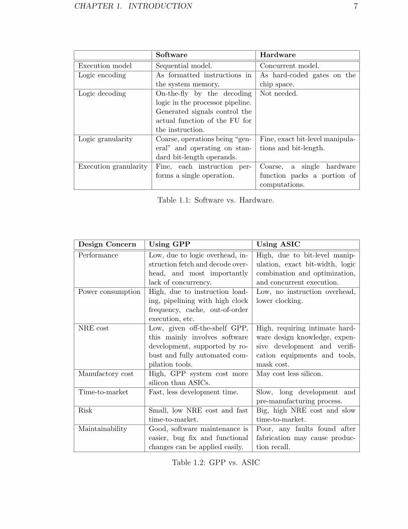
1.1.3 Software vs. Hardware
The differences between software and hardware are further elaborated in Table 1.1.
Table 1.2 summarizes and expands a little on the general pros and cons of using
GPPs or ASICs over common design concerns.
As we can imagine, GPPs and ASICs sit at the very two ends of the spectrum
with exactly opposite pros and cons. Either choice causes sacrifice of the benefits
from the other one. Consequently, the current industrial practice couples GPPs and
ASICs to different extents so as to take advantage of the combined strength, yielding
a spectrum of possible choices.
1.1.4 Spectrum of Specializations
Specialized circuits can be integrated to cooperate with the processor at various lev-
els. Fine grained specialization can be done at the instruction level of the processor.
In this way, frequently occurring computational patterns (which include multiple
operations) can be executed more efficiently as complex instructions in specialized
functional units directly on the processor’s datapath.
2Mask process creates photographic molds for multi-layered IC, and is usually very expensive.3NRE refers to the one-time cost of researching, designing, and testing a new product, and is
supposed to be amortized in the later per-product sales.
CHAPTER 1. INTRODUCTION 7
Software Hardware
Execution model Sequential model. Concurrent model.Logic encoding As formatted instructions in
the system memory.As hard-coded gates on thechip space.
Logic decoding On-the-fly by the decodinglogic in the processor pipeline.Generated signals control theactual function of the FU forthe instruction.
Not needed.
Logic granularity Coarse, operations being “gen-eral” and operating on stan-dard bit-length operands.
Fine, exact bit-level manipula-tions and bit-length.
Execution granularity Fine, each instruction per-forms a single operation.
Coarse, a single hardwarefunction packs a portion ofcomputations.
Table 1.1: Software vs. Hardware.
Design Concern Using GPP Using ASIC
Performance Low, due to logic overhead, in-struction fetch and decode over-head, and most importantlylack of concurrency.
High, due to bit-level manip-ulation, exact bit-width, logiccombination and optimization,and concurrent execution.
Power consumption High, due to instruction load-ing, pipelining with high clockfrequency, cache, out-of-orderexecution, etc.
Low, no instruction overhead,lower clocking.
NRE cost Low, given off-the-shelf GPP,this mainly involves softwaredevelopment, supported by ro-bust and fully automated com-pilation tools.
High, requiring intimate hard-ware design knowledge, expen-sive development and verifi-cation equipments and tools,mask cost.
Manufactory cost High, GPP system cost moresilicon than ASICs.
May cost less silicon.
Time-to-market Fast, less development time. Slow, long development andpre-manufacturing process.
Risk Small, low NRE cost and fasttime-to-market.
Big, high NRE cost and slowtime-to-market.
Maintainability Good, software maintenance iseasier, bug fix and functionalchanges can be applied easily.
Poor, any faults found afterfabrication may cause produc-tion recall.
Table 1.2: GPP vs. ASIC

CHAPTER 1. INTRODUCTION 8
DSPRISC CISC ASICLoosely coupledProcessor + ASIC
Processor +Coprocessor
Software Hardware
SIMD
Fine grained specialization
Coarse grained specialization
PerformanceFlexibility
ASIP
Figure 1.3: Spectrum of system specialization.
CISC, DSP, SIMD, ASIP architectures in Figure 1.3 are light weight fine grained
specialization of processor’s instruction set. For a RISC (Reduced Instruction-set
Computer) processor on the leftmost side, each operation is executed with a sin-
gle word-level instruction. A CISC (Complex Instruction-set Computer) processor
allows a computational instruction to operate directly on operands in the system
memory. This essentially is a coarser grained instruction consisting of both the
memory access operations for the operands and the computational operation.
Digital Signal Processors (DSP) employ the single cycle MAC (Multiply-Accumulate)
instruction to accelerate intensive product accumulations, i.e., Sum =∑Xi ∗ Yi. A
MAC instruction computes the repeating pattern Sumi = Xi ∗ Yi + Sumi−1 each in
a single cycle, and accumulate the sum in an internal register progressively in the
MAC unit. Note that in a GPP, the same pattern will be executed as a multiply in-
struction (maybe multi-cycle) followed by an add instruction, with the result of each
instruction output to the register file. The block diagram and computation logic of
a MAC unit are depicted in Figure 1.4. In order to achieve high performance, MAC
units often use high speed combinational multipliers at the cost of the number of
transistors.
Unlike collapsing data dependent operations as the MAC instruction, a SIMD
(Single Instruction, Multiple Data) architecture exploits the parallelism among the
operations. A single SIMD instruction applies the same operation on several in-

CHAPTER 1. INTRODUCTION 9
(a) (b)
XY
Output
OutputRegister
Multiplier
Accumulator
MAC Unit*
+
*+
Xi Yi
Xi+1 Yi+1
Sumi-1
Sumi
Sumi+1
Figure 1.4: MAC in a DSP. (a) Chaining basic operations on the dataflow, (b) Blockdiagram of a MAC unit.
dependent data sources concurrently. Instructions of this kind are employed in
supercomputers for long vector operations in scientific computation. They are also
widely adapted in multimedia instruction-set extensions, such as MMX, SSE and
3DNOW!, to enhance short vector operations in multimedia and communication
applications. SIMD units are usually assisted by wide registers and register ports
for larger operand bandwidth.
ASIPs (Application Specific Instruction-set Processor) have their instruction-
set tailored to a specific application or application domain. For example, special
instructions are used in processors specialized in encryption for bit permutation and
s-box operations [72], and in fast fourier transform to perform or assist butterfly
operations [52]. In fact, DSPs and SIMDs are instances of ASIPs originally in the
domain of digital signal processing and scientific computation, even though their
functions tend to become an integral part of general purpose processors for wide
range of consumer applications.
In a coarse grained specialization approach, computationally intensive tasks or
kernel loops are mapped to the hardware, loosely coupled with the host processor as

CHAPTER 1. INTRODUCTION 10
a co-processor. The host processor works with the co-processor in a “master/slave”
fashion. Special communication instruments are used for data transfer and syn-
chronization via system bus or network in between. The co-processor has a higher
degree of independence but it incurs longer communication latency with the proces-
sor, compared to specialized functional units. Computation kernels mapped to the
co-processor usually require intensive algorithmic and hardware oriented optimiza-
tions to exploit full performance potential. In this sense, the intimate knowledge of
hardware and effort required from the designers and tools are comparable to that of
a pure ASIC design. However, the decoupling of computation kernels does provide
opportunities of reusing the hardware component. Through proper parametrization
and interfacing, verified high performance hardware components of useful algorithms
can be plugged into a different system with less design and manufacturing effort.
An example of loosely coupled hardware module is reviewed in Section 2.1.2.
In general, specialization on larger execution granularity carries more perfor-
mance advantages. More effort, mainly focusing on loop transformation and op-
timization to expose more parallelism or even algorithm changes to adapt to the
concurrent execution model, is needed to achieve optimized performance. On the
other hand, fine grained specialization is more flexible, as smaller computation pat-
terns strike a more balanced distribution of software/hardware execution, and can
be reused wherever they appear. Computation patterns can be deduced from the
software implementation of the application, which fits well in the software compila-
tion process. The trade-off goes to the less performance gain compared to a coarse
grained approach.

CHAPTER 1. INTRODUCTION 11
LogicBlock
LogicBlock
LogicBlock
LogicBlock
LogicBlock
LogicBlock
LogicBlock
LogicBlock
LogicBlock
I/O pin
RoutingResources
i0
MUXi2i1
i3out
SRAM bits
(a)
4-input LUT
4-inputLUT Reg
outinputs
(b)
i0i1i2i3
Logic Block
Clock
Figure 1.5: General structure of a FPGA.
1.1.5 FPGAs and Reconfigurable Computing
Coupling hard-wired logic with microprocessors strikes the balance between perfor-
mance and design effort. However, it does not break the “fixed once fabricated”
model. A more flexible solution has only unfolded with recent availability of high
density, high performance reconfigurable hardware, which is capable of being re-
programmed conveniently and swiftly after fabrication. Reconfigurable hardware is
also able to achieve high performance through concurrent execution model of com-
putation. Therefore, it is considered as the glue technology connecting the worlds of
software and hardware. The methodologies and applications of utilizing hardware
reconfigurability are known as Reconfigurable Computing .
The basis of reconfigurable computing is reconfigurable devices, a common ex-
ample being Field-Programmable Gate Arrays (FPGAs). As indicated with the
phrase “Field-Programmable”, the functionality of an FPGA can be determined
on-site, rather than at the time of its fabrication. An FPGA contains an array of
small computational elements known as logic blocks, surrounded and connected by
programmable routing resources. The functionality of logic blocks and connectivity
of routing resources are determined through multiple programmable configuration
CHAPTER 1. INTRODUCTION 12
points. Each configuration point is associated with SRAM bits in SRAM based
FPGAs. Reconfiguration is merely the process of loading organized bitstream to
the SRAM. Figure 1.5 shows the general structure of a FPGA. In a real product,
hundreds of thousands of logic blocks can be integrated on a single chip (e.g., 330K
logic blocks on a Xilinx Virtex-5 chip [41] comparable roughly to the logic capacity
of a million gates), onto which even large and complex algorithms can be mapped.
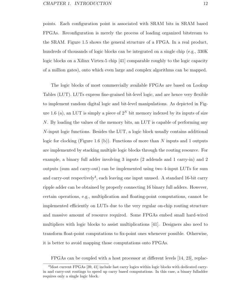
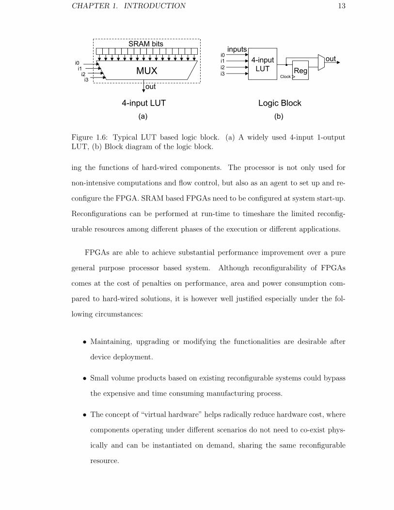
The logic blocks of most commercially available FPGAs are based on Lookup
Tables (LUT). LUTs express fine-grained bit-level logic, and are hence very flexible
to implement random digital logic and bit-level manipulations. As depicted in Fig-
ure 1.6 (a), an LUT is simply a piece of 2N bit memory indexed by its inputs of size
N . By loading the values of the memory bits, an LUT is capable of performing any
N -input logic functions. Besides the LUT, a logic block usually contains additional
logic for clocking (Figure 1.6 (b)). Functions of more than N inputs and 1 outputs
are implemented by stacking multiple logic blocks through the routing resource. For
example, a binary full adder involving 3 inputs (2 addends and 1 carry-in) and 2
outputs (sum and carry-out) can be implemented using two 4-input LUTs for sum
and carry-out respectively4, each leaving one input unused. A standard 16-bit carry
ripple adder can be obtained by properly connecting 16 binary full adders. However,
certain operations, e.g., multiplication and floating-point computations, cannot be
implemented efficiently on LUTs due to the very regular on-chip routing structure
and massive amount of resource required. Some FPGAs embed small hard-wired
multipliers with logic blocks to assist multiplications [41]. Designers also need to
transform float-point computations to fix-point ones whenever possible. Otherwise,
it is better to avoid mapping those computations onto FPGAs.
FPGAs can be coupled with a host processor at different levels [14, 23], replac-
4Most current FPGAs [39, 41] include fast carry logics within logic blocks with dedicated carry-in and carry-out routings to speed up carry based computations. In this case, a binary fulladderrequires only a single logic block.
CHAPTER 1. INTRODUCTION 13
LogicBlock
LogicBlock
LogicBlock
LogicBlock
LogicBlock
LogicBlock
LogicBlock
LogicBlock
LogicBlock
I/O pin
RoutingResources
i0
MUXi2i1
i3out
SRAM bits
(a)
4-input LUT
4-inputLUT Reg
outinputs
(b)
i0i1i2i3
Logic Block
Clock
Figure 1.6: Typical LUT based logic block. (a) A widely used 4-input 1-outputLUT, (b) Block diagram of the logic block.
ing the functions of hard-wired components. The processor is not only used for
non-intensive computations and flow control, but also as an agent to set up and re-
configure the FPGA. SRAM based FPGAs need to be configured at system start-up.
Reconfigurations can be performed at run-time to timeshare the limited reconfig-
urable resources among different phases of the execution or different applications.
FPGAs are able to achieve substantial performance improvement over a pure
general purpose processor based system. Although reconfigurability of FPGAs
comes at the cost of penalties on performance, area and power consumption com-
pared to hard-wired solutions, it is however well justified especially under the fol-
lowing circumstances:
• Maintaining, upgrading or modifying the functionalities are desirable after
device deployment.
• Small volume products based on existing reconfigurable systems could bypass
the expensive and time consuming manufacturing process.
• The concept of “virtual hardware” helps radically reduce hardware cost, where
components operating under different scenarios do not need to co-exist phys-
ically and can be instantiated on demand, sharing the same reconfigurable
resource.

CHAPTER 1. INTRODUCTION 14
• For an application with certain data values changing slowly over time, e.g., a
key-specified encrypter, the set of values lasting for a period of time can be
used to create an optimized configuration for the time window. By treating
those data values as constants, logic of the configuration can be greatly sim-
plified through partial evaluation techniques. As inputs are instantiated, such
a customized system may achieve even higher performance than the ASICs.
1.2 Instruction-set Extensible Processors
The efforts of this thesis go to the fine grained specialization of the processor’s
instruction-set. In particular, we focus on the processors with configurable instruction-
set. Such a processor core is usually divided into two parts: the static logic for the
basic ISA, and the configurable logic for the application specific instructions. The
configurable part of the processor can either be implemented in reconfigurable logic
for flexibility and run-time reconfigurability, or hard-wired for higher performance
and lower power consumption. In either case, with well defined hardware interfaces
between the two parts, the complexity of the design effort to tailor the processor for
a particular application is narrowed down to defining the new instructions [47].
As the set of configurable application specific instructions is usually referred to
as the Instruction-set Extension (ISE), we call such a processor, under the category
of ASIP, an Instruction-set Extensible Processor (ISEP), or Extensible Processor.
While instructions from the basic ISA are base instructions, an instruction cus-
tomizable for specific applications is a Custom Instruction.
The general architecture of an extensible processor is shown in Figure 1.7. Cus-
tom Functional Units (CFU) are integrated in the base processor core at the same
level as other base functional units, and access the input and output operands stored

CHAPTER 1. INTRODUCTION 15
CPU
+ + LD/ST CFU1 CFU2
Register files
Instruction dispatcherAND AND
ORAND2_OR
(a) (b)
*
Figure 1.7: General architecture of instruction-set extensible processors. (a) Cus-tom functional units (CFU) embedded in the processor datapath, (b) A complexcomputation pattern encapsulated as a custom instruction.
in the register file. A custom instruction is an encapsulation of a frequently occur-
ring computation pattern involving a cluster of basic operations (see Figure1.7(b)),
and can be executed with a single fetch-decode-execute pass. Hardware implementa-
tion of the operation cluster with the CFU exploits the concurrency among parallel
operations (e.g., the two ANDs in Figure1.7(b)), optimizes performance of chained
(dependent) operations at the gate level (e.g., a 3-input adder); thus it is able to
improve the overall execution time. Besides, as the clock period of the processor
pipeline is often not constrained by the ALUs5, the increase of actual latency of
the combined logic may not prolong the clock period or require extra cycles. For
example, logic operations as in Figure 1.7(b) are only one level logic, and several of
them can be easily chained within a clock period.
A custom instruction may require more input and output operands than the
typical 2-input 1-output instructions; but it also brings about better register usage
by eliminating the need to output intermediate values, which otherwise need to
5For example, the out-of-order issue logic of a superscalar processor often becomes the bottleneckfor the clock period since its latency increases quadratically with the size of the issue window [78].Also, while gate level logic benefits much from process technology advances, bypass network latencydoes not [62], and can become the bottleneck as well. After all, most processors run at frequencieslower than their technology limits. For portable embedded systems, a slower clock frequency isoften required and essential to reduce power consumption. Reduced execution overhead due tocustom instructions also creates opportunities to lower the clock frequency.

CHAPTER 1. INTRODUCTION 16
be written back to the register file (e.g., the results of the two AND operations in
Figure 1.7(b)). The denser code leads to smaller code size. Energy consumption
can also be reduced due to improved memory hierarchy performance (code size
reduction, less cache footprints) and other factors mentioned earlier.
In specific designs, coarser grained ALU based logic blocks can be used to imple-
ment the reconfigurable CFUs, trading off bit-level manipulation flexibility against
faster reconfiguration and execution performance. Instead of using a single unified
register file with large number of read/write ports for CFU inputs and outputs,
multiple or dedicated register banks can be used. The design space has conflicting
objective functions such as performance, flexibility and complexity. We will study
specific extensible processors and some of the design options later in Chapter 3.
1.2.1 Hardware-Software Partitioning
The main design effort of tailoring an extensible processor is to define the custom
instructions for the given application to meet design goals. Identifying suitable
custom instructions is the hardware-software partitioning process that divides the
computations between the processor execution (using base instructions) and hard-
ware execution (using custom instructions). Various design constraints must be
satisfied in order to deliver a viable system, including performance, silicon area
cost, power consumption and architectural limitations. This problem is frequently
modeled as a single objective optimization procedure by optimizing a certain as-
pect (usually performance), while putting constraints on the others. Specifically,
the custom instruction identification process extracts suitable computation patterns
from the application to derive the ISE for the maximal performance under design
constraints.

CHAPTER 1. INTRODUCTION 17
A general hardware-software partitioning practice usually starts with the soft-
ware implementation of the application written in high-level languages (e.g., C/C++,
FORTRAN). The application is compiled, and profiled by executing it with typical
data sets on the target processor. Based on the profiling information, hot spots,
which occupy noticeable potions of the total execution time, are located. These hot
spots indicate the code locations that may benefit from hardware execution, and
are candidates for hardware implementations. The designer then tries to map the
functionality corresponding to the hot spots to hardware (custom instructions, in
our case). If the hardware area exceeds the preset budget, the designer will need
to optimize the hardware functions for area while possibly trading off some per-
formance. Unfortunately, the process of mapping software code to the hardware is
tedious, time consuming and highly dependent on the knowledge of the designer.
Although an experienced designer can even perform algorithmic changes to expose
more opportunities for efficient hardware implementation, regularities embedded
inside large and complicated computation paths are sometimes hard to discover.
Manual effort is therefore unlikely to cover the computation optimally with limited
hardware resource.
In order to overcome these difficulties of manual partitioning, we present a com-
piler based automatic custom instruction identification flow. In a software devel-
opment environment, the compiler breaks down high-level language statements into
basic operations and map these operations to processor instructions to produce the
machine executable. In our design flow, the compiler in addition performs ISE iden-
tification to find suitable computation patterns and generates the executable with
custom instructions. Instead of manual algorithmic changes, we rely on modern
compiler transformations to expose potential parallelism among base operations.
Large computation paths can be efficiently explored by methodologies devised in
this thesis. Software programmers can also easily adapt to the ISEP design flow

CHAPTER 1. INTRODUCTION 18
without in depth hardware knowledge.
1.2.2 Compiler and Intermediate Representation
A generic compiler processes the code of the application as follows. High-level
language statements are first transformed by the compiler front-end to the Inter-
mediate Representation (IR), structured internally as graphs. Various analysis and
re-arrangements of operations known as machine independent optimizations are car-
ried out on the IR. Then, the back-end of the compiler generates binary executables
for the target processor by binding IR objects to actual architectural resources, op-
erations to instructions, operands to registers or memory locations, concurrencies
and dependencies to time slots, through instruction binding, register allocation, and
instruction scheduling, respectively. Various machine dependent optimizations are
also performed at the back-end.
The IR consists of Control Flow Graph (CFG) and Dataflow Graph (DFG,
also called Data Dependence Graph) that are used for the ISE identification. CFG
expresses the structure of the application’s logic flow (if-else, loops and function
calls) by partitioning the code into basic blocks over control flow altering operations,
i.e., jumps and branches. An edge between two basic blocks indicates a possible
control flow direction to take, depending on the outcome of the branch condition
(if any). For each basic block, DFG is constructed to express the dataflow6, with
operations as nodes and edges attributing the dependencies among the operands.
Figure 1.8 shows an example of CFG and DFG corresponding to a code segment. For
a GPP, each operation on the DFG is usually covered with one machine instruction
6A basic blocks is the basic unit for instruction scheduling because control flow within it does notchange. However, basic blocks are usually very small (average 4-5 instructions each) and severelyconstraint the performance of modern Instruction Level Parallelism processors (superscalars andVLIWs). Larger blocks containing multiple basic blocks, e.g., traces, superblocks and hyperblocks,are exploited with architectural support. DFGs can be built upon those blocks as well. We willsee how custom instructions can be used in those cases in Section 2.2.2.

CHAPTER 1. INTRODUCTION 19
int f(f_no, x, y, z)int f_no, x, y, z;
{int res;if(f_no==1)
res = (x & y) | (~x & z);else
res = x ^ y ^ z;return res;
}
. . .if (f_no==1)
res = (x & y) | (~x & z);
res = x ^ y ^ z;
return res;
BB0
BB1
BB2
BB3
&
y x
z~&
|
res
BB1
(a) (b) (c)
Figure 1.8: Intermediate representation. (a) Source code of a function (adaptedfrom Secure Hash Algorithm), (b) Its control flow graph, (c) Dataflow graph ofbasic block 1.
during instruction binding. However, a custom instruction intends to cover a cluster
of operations and is hence captured as a Subgraph of the DFG.
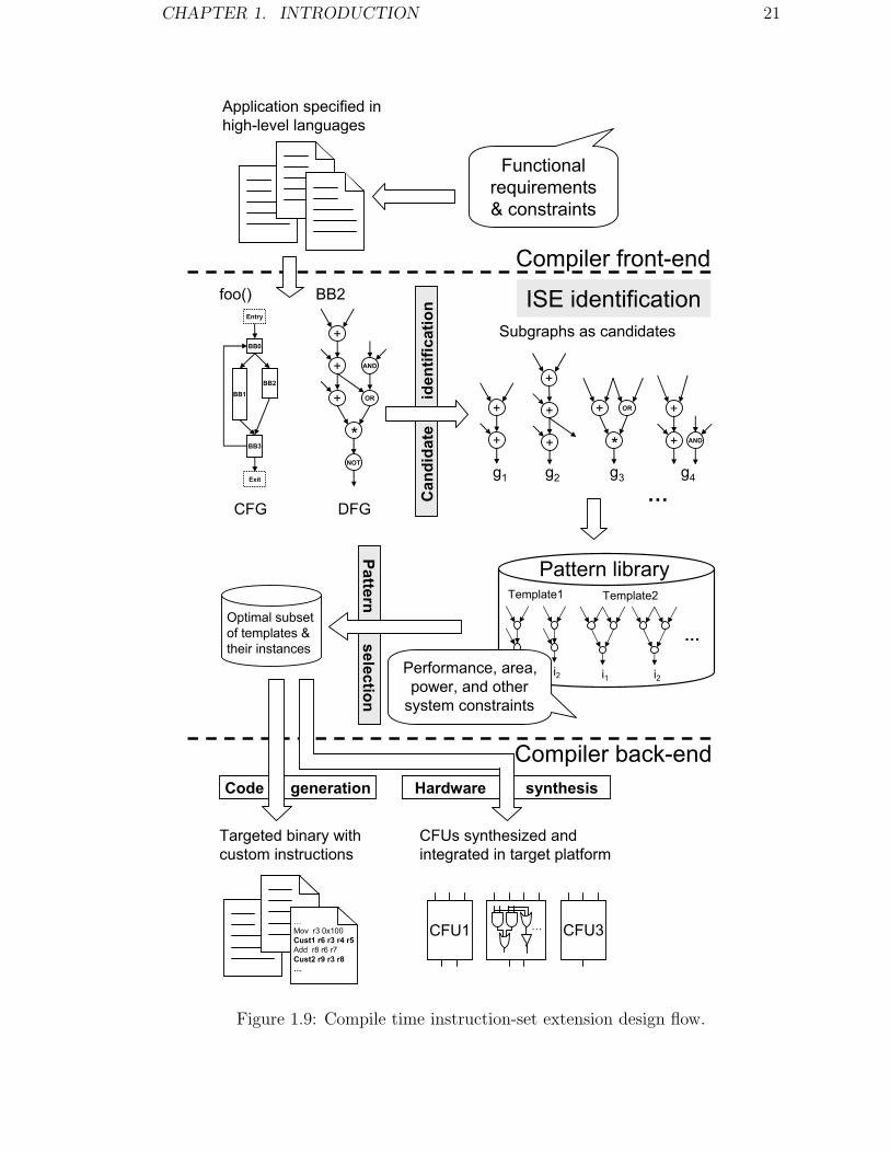
1.2.3 An Overview of the Design Flow
In our design flow, the compiler should perform three additional tasks: identify-
ing the ISE, generating the binary executables under the new instruction-set, and
producing the new CFUs.
ISE identification is essentially a problem of regularity extraction, which at-
tempts to find common substructures in a set of graphs. Topologically equivalent
DFG subgraphs perform the same logic function, forming a template pattern for a
potential custom instruction. Each occurrence is an instance of the template. The
target of ISE identification problem is to find a small number of templates along
with their instances to cover the DFGs for the fastest execution. This problem
involves the following two subproblems. (1) Candidate pattern enumeration — enu-
merate a set of subgraphs from the application’s DFG and build the pattern library
of templates and their instances. (2) Custom instruction selection — evaluate each
candidate in the library and select an optimal subset under various design con-

CHAPTER 1. INTRODUCTION 20
straints. The first subproblem is a subgraph enumeration problem, while the second
is an optimization problem.
The work flow of the partitioning process is depicted in Figure 1.9. ISE identifi-
cation is plugged in between the compiler front-end and back-end. Heavily executed
hot spots of the application, identified through program profiling, are processed by
ISE identification algorithms. The resultant templates are then passed to the com-
piler back-end. During instruction binding, the instances of these templates will
be mapped to custom instructions, either by simple peephole substitution or by
the pattern matcher that recognizes the new templates, to produce the executables.
Hardware description of the templates are generated and fed to the synthesis tool
chain to build the CFUs on the target hardware. Decoding logic of the processor
also needs to be modified for the new instructions.
1.3 Contributions and Organization of this Thesis
The main contributions of this thesis are the efficient and scalable custom instruc-
tion identification methodologies. The capabilities of handling very large dataflow
graphs and subgraphs with relaxed architectural constraints are essential for the
custom instructions to exploit greater parallelism and operation chaining oppor-
tunities exposed by modern compiler transformations. Thus it is crucial for the
automatic design flow to generate high quality solution for the given application.
Specific contributions are listed as follows:
1. We present efficient and scalable subgraph enumeration algorithms for the
candidate pattern enumeration problem. Through exhaustive enumeration,
isomorphic subgraphs embedded inside the dataflow graphs, which can be
CHAPTER 1. INTRODUCTION 21
CFU3CFU1
Hardware synthesisCode generation
Application specified in high-level languages
foo()
BB1BB2
BB0
BB3
Entry
Exit
CFG
+ AND
+
OR+
NOT
*
BB2
DFG
Compiler front-end
Subgraphs as candidates
+
+
g1
+
+
+
g2
OR+
*g3
+ AND
+
g4
…Can
dida
te
id
entif
icat
ion
…
i1
Template1
i2 i1
Template2
i2
Pattern library
Pattern selection
Optimal subset of templates &their instances
Compiler back-end
Targeted binary withcustom instructions
…Mov r3 0x100Cust1 r6 r3 r4 r5Add r8 r6 r7Cust2 r9 r3 r8…
…
CFUs synthesized and integrated in target platform
Functional requirements & constraints
Performance, area, power, and other
system constraints
ISE identification
Figure 1.9: Compile time instruction-set extension design flow.
CHAPTER 1. INTRODUCTION 22
covered by the same custom instructions, are fully exposed to the selection
process. Our custom instruction selection method based on integer linear
programming (ILP) is able to exploit subgraph isomorphism optimally. Given
this, the resulting effect indicates that a small set of custom instructions can
usually achieve most performance improvement of the applications.
2. Based on our custom instruction identification methodology, we then con-
duct a systematic study of the effects and correlations between various design
constraints and system performance on a broad range of embedded bench-
mark applications. In particular, a dynamic execution trace based method is
adapted to broaden the scope of custom instruction identification beyond ba-
sic blocks, which allows us to characterize the limit potential of using custom
instructions. This study provides a valuable reference for the design of general
extensible processors.
3. We explore a novel application of using custom instructions to meet timing
constraints of real-time systems. Custom instructions are selected using a
modified ILP formulation to minimize the worst-case execution time of the
application. We also devise high quality heuristic selection algorithms to avoid
the complexity of solving ILP formulations, which yield identical selections to
the optimal ones most of the times within very short run time.
This thesis is organized as follows. We discuss existing extensible processors
and several important design issues in Chapter 2 in order to provide a more compre-
hensive background for the ISEP scene. Related works on the custom instruction
identification problem are reviewed in Chapter 3. In Chapter 4, we present the
scalable subgraph enumeration algorithms for the candidate pattern enumeration
problem. We describe the optimal custom instruction selection based on integer
linear programming in Chapter 5. In the same chapter, we present the study on

CHAPTER 1. INTRODUCTION 23
the performance impact using custom instructions under various design constraints.
Methodologies of applying custom instructions to improve worst-case execution time
for real-time applications are presented in Chapter 6. Finally, Chapter 7 concludes
the thesis.
Chapter 2
Instruction-Set Extensible
Processors
A huge gap exists between what we know is possible with today’s ma-
chines and what we have so far been able to finish. – Donald E. Knuth
We review previous works on instruction-set extensible processors in this chap-
ter. Note that this review does not intend to be exhaustive, but highlights different
options and important design issues, and serve as a more comprehensive background
of the ISEP scene.
2.1 Past Systems
The order of the presentation in this section shows the trace of system evolvement.
We study seven systems, which grow in features and sophistication. The focus of
systems with reconfigurable ISE are mainly on the architecture design of effective re-
configurable CFUs that can be swiftly reconfigured, and relaxing the I/O constraints
24
CHAPTER 2. INSTRUCTION-SET EXTENSIBLE PROCESSORS 25
of the CFUs. The focus of configurable extensible processors with synthesized CFUs
are on the design environment which provides a high-level interface to specify the
logic of custom instructions and evaluate their effects, the automatic generation of
the compilation tool chain and hardware descriptions. The techniques studied in
this section merely show the possibilities. Again, a real life extensible processor is a
trade-off among different aspects, satisfying various design constraints.
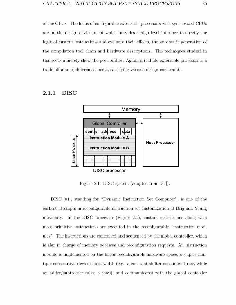
2.1.1 DISC
Global Controller
Line
ar H
W s
pace
Memory
Host Processor
DISC processor
control address data
Instruction Module B
Instruction Module A
Figure 2.1: DISC system (adapted from [81]).
DISC [81], standing for “Dynamic Instruction Set Computer”, is one of the
earliest attempts in reconfigurable instruction set customization at Brigham Young
university. In the DISC processor (Figure 2.1), custom instructions along with
most primitive instructions are executed in the reconfigurable “instruction mod-
ules”. The instructions are controlled and sequenced by the global controller, which
is also in charge of memory accesses and reconfiguration requests. An instruction
module is implemented on the linear reconfigurable hardware space, occupies mul-
tiple consecutive rows of fixed width (e.g., a constant shifter consumes 1 row, while
an adder/subtracter takes 3 rows), and communicates with the global controller

CHAPTER 2. INSTRUCTION-SET EXTENSIBLE PROCESSORS 26
through the underlining bus. The instruction modules are also relocatable, such
that they can fit into consecutive rows available anywhere on the RA (Reconfig-
urable Array). In fact, the row based RA design turns out to be very effective for
relatively small dataflow computations due to its simplicity and predictable timing
model, and is adapted in most later systems, such as Garp [34], PRISC [70] and
Chimaera [82].
At run time, the global controller takes an instruction from the memory, exe-
cutes it if its corresponding instruction module is available. Otherwise, the global
controller halts the execution, and sends a request to the host processor for the
missing instruction module. According to the current status of the resource occu-
pation, the host processor either allocates the rows if available, or free up other
instruction modules using simple LRU (Least-Recently-Used) algorithm to make
room for the new instruction module. After the instruction module is loaded from
the pre-synthesized instruction library to the allocated space of the RA, the global
controller resumes execution.
The problem of DISC is its uniform treatment of custom instructions and simple
primitive instructions. Primitive operations executing on hard-wired ALUs can be
more efficient than executing them on reconfigurable logic. Executing primitive
operations on hard-wired ALUs will also reduce the complexity of run-time resource
management. The full fledged host processor used for only resource allocation and
reconfiguration is highly under utilized. Instead, a much simpler processor, even
integrated with the global controller, can achieve the same functionality.
2.1.2 Garp
The Garp project at UC Berkeley [34] has a similar reconfiguration array architec-
ture as DISC (linear hardware space and row based reconfiguration), and addresses
CHAPTER 2. INSTRUCTION-SET EXTENSIBLE PROCESSORS 27
several of DISC’s limitations. Instead of executing primitive operations on the RA,
the host – a MIPS II processor takes over the primitive operations. The MIPS
II instruction set is augmented to manage the RA. There is no explicit run-time
resource management in Garp, partially because mapping only the computational
intensive kernels reduces total resource requirement and hence configuration swaps.
In addition, Garp can cache upto four configurations, allowing fast configuration
switches in a transparent fashion. This way, resource management is replaced by
cache management.
Some additional instructions are added to the MIPS II core to control the RA.
A configuration in the main memory is loaded (or switched to if cached) through
a gaconf instruction. Input data is set up by mtga instructions, which transfers
the value of a MIPS II register to an RA register. Meanwhile, mtga is able to set
the internal clock counter of RA to a positive value, indicating the cycles needed to
complete the custom function. Finally, mfga waits the counter to decrease to zero,
and reads the result data back to a MIPS II register from an RA register.
As the RA has no direct access to MIPS II registers, small dataflow graph com-
putation would carry communication overhead due to the use of explicit data transfer
instructions (e.g., mtga and mfga). This may offset the performance improvements.
In fact, the RA is built with direct access to the memory, targeting coarser grained
innermost loop computations [13], where communication overhead can be amortized.
Although the RA in DISC processor also has memory access (through the global
controller), all instruction modules (primitive and custom operations) are architec-
turally equal. In contrast, custom functions in Garp are executed differently from
the normal instructions; the RA works more like a slave to the MIPS II processor.
Technically, Garp is a loosely coupled reconfigurable architecture. However, the im-
provements over DISC project as suggested above do provide useful guidelines for
later extensible processor designs.

CHAPTER 2. INSTRUCTION-SET EXTENSIBLE PROCESSORS 28
RegisterFileand
BypassLogic
FU1 FU2 PFU
Result operand bus
Source operands bus
Paddr
Pdata
expfu rs rt rd LPnum
6 5 5 5 11
(a) (b)
expfu : opcode of the FPUrs, rt : fields of source registersrd : field of destination registerLPnum : FPU configuration specifier
Figure 2.2: PRISC system (adapted from [70]). (a) Datapath, (b) Format of the32-bit FPU instruction.
2.1.3 PRISC
PRISC (PRogrammable Instruction Set Computer) [70] is the very first work that
defines the typical architectural of an ISEP (see Section 1.2). As depicted in Fig-
ure 2.2(a), a single 2-inputs 1-output PFU (Programmable Functional Unit) is added
at the execution stage of a RISC processor pipeline in parallel with standard FUs.
The PFU behaves the same way as other FUs that have direct access to the register
file and bypassing network, and is restricted to 1 cycle execution latency for simpler
synchronization.
The PFU instruction is encoded with a standard 32-bit format shown in Fig-
ure 2.2(b). expfu is the opcode triggering the PFU, while LPnum specifies a certain
PFU configuration, each corresponding to a different custom function. At run time,
the current PFU configuration specifier is hold in a special 11-bit register. A mis-
match between the register and the LPnum field of a PFU instruction causes an
exception. The exception handler will then reconfigure the PFU to the configura-
tion specified by LPnum, and update the special register accordingly. Configuration
bits are sent to the PFU via Paddr and Pdata ports (Figure 2.2(a)). This is done
either by the processor using augmented load instructions sequentially for a low
speed solution, or by a dedicated configuration controller with fast memory access
CHAPTER 2. INSTRUCTION-SET EXTENSIBLE PROCESSORS 29
for a high speed solution. The minimum reconfiguration latency is reported to be
around 100 cycles. As there is only 1 PFU and configuration switches within a loop
body is highly undesirable, a 1 configuration per loop restriction is imposed.
Automatic but straight forward hardware-software partitioning is used to group
operations for the PFU. At first, the operations of the target application are ana-
lyzed, and the ones not suitable for mapping to the PFU are marked (i.e., memory
operations, floating-point operations, multiplication and division). Starting with a
suitable operation on the dataflow graph, the algorithm follows the data dependen-
cies backwards and greedily includes suitable operations in the function along the
way. The backward traversal terminates when the next operation is a non-suitable
one, or including it yields a function requiring more than 2 source operands or more
than 1 destination operand. The resultant group of suitable operations is called a
maximal, and will be fed to the hardware synthesizer to produce the corresponding
configuration image.
The main limitation of PRISC is that the PFU is restricted to 2-input 1-output
functions. Even though this simplifies operands encoding and minimizes modifi-
cation to the register file, it severely restrains the PFU from implementing larger
groups of operations with more number of input/output operands which stand for
higher performance improvements. Furthermore, no reuse of equivalent logic func-
tion at different locations with the same PFU is considered, even though encoding
input/output registers in the PFU instruction format already provides this flexibil-
ity. However, this kind of reuse may not really be beneficial due to the single PFU
setup, unless the equivalent functions occur consecutively without being replaced by
the other configurations in the middle.
CHAPTER 2. INSTRUCTION-SET EXTENSIBLE PROCESSORS 30
RFUOP dest reg RFUOP number
10 5 17
RFUOP : opcode of the RFU
dest reg : destintation register number in the host register file
RFUOP number : RFU function specifier
(b)
HostProcessorPipeline
Register File
Configuration & Caching Unit
Reconfigurable Array
Shadow Register File
R0,
…,R
8
…
Exe
c. C
trl U
nit
Internal Bus
Cache interface
inputs outp
ut
(a)
Figure 2.3: Chimaera system (adapted from [82, 33]). (a) Block diagram, (b)RPUOP instruction format.
2.1.4 Chimaera
The Chimaera reconfigurable functional unit [82, 33] (RFU) developed at North-
western University is inspired by PRISC, but is more sophisticated and integrated
inside an out-of-order superscalar processor core. The main innovation of the Chi-
maera RFU is its capability of using up to 9 input registers and producing 1 result
in an output register. This is achieved through a special design of the RA, where
the values of all the registers (in fact the shadow registers in Figure 2.3(a)) are
propagated through out the RA and hard-wired in the configurations so that they
can be accessed simultaneously (see [82] for details). Hard-wiring the inputs on the
one hand eliminates the need of encoding input registers explicitly in the RFU in-
struction (see the instruction format in Figure 2.3(b)). In fact, it is not possible to
encode so many input operands in a single 32-bit instruction. On the other hand,
as a trade-off, RFU instructions cannot be reused upon any changes in the input
operands. This inflexibility is partially compensated by accommodating multiple
RFU configurations on the RA, with its resource managed by the configuration and
caching unit (similar to the DISC processor).
In order to interface with the out-of-order core, a shadow register file of size equal

CHAPTER 2. INSTRUCTION-SET EXTENSIBLE PROCESSORS 31
input1 input2 input3 input4
output1 output2
CCA
(a)
ID
EX
MEM
WB Control Generator
CCA configcache
CCA
@ 1 R1, R6, R8
Branchtarget
Configcacheentry
Inputregisters
BTB
…
(b)
Figure 2.4: The CCA system (adapted from [21, 20]). (a) The CCA (ConfigurableCompute Accelerator), (b) System architecture.
to the number of logical registers (9, in Chimaera) is used1. A shadow register is
read-only to the RA and is synchronized with the corresponding physical register for
the RFU operation through the register renaming logic. The single result is written
back to the host register file like normal instructions. Due to register renaming,
extra read/write ports must be added to the host register file to communicate with
the RA, which implies drastic increase in power and area of the host register file.
However, cost is a secondary concern in the design of Chimaera.
2.1.5 CCA
A CCA (Configurable Compute Accelerator) is used instead of the reconfigurable
array in the system developed at University of Michigan [21, 20]. Unlike the fine-
grained configurable RA, CCA is composed of a layered network of FUs, each capable
of several fast word-level dataflow operations, i.e., logical, addition/subtraction,
move or shift (see Figure 2.4(a)). The function of each FU and their connectivity
1In a out-of-order core, usually there are more physical registers than logical registers to solvefalse dependencies through register renaming.

CHAPTER 2. INSTRUCTION-SET EXTENSIBLE PROCESSORS 32
can be specified by only a few bits, while hundreds are needed in an LUT based
RA. Coarser logic granularity guarantees faster reconfiguration time. In fact, the
whole CCA can be defined using around 200 bits, such that configuring the CCA
on-the-fly with control signals rather than writing to the associated SRAM is made
possible2. The trade-off here is that the CCA is unable to exploit bit/sub-word
level optimizations, and only the subgraphs, which are able to fit in the fixed CCA
topology, can be used.
In the first CCA system, the CCA configuration is conventionally encoded in the
instruction stream [21]. Under the assumption of a Pentium P6 microarchitecture,
where a µop takes 118 bits, each custom instruction can be encoded with 2 consec-
utive µops. However, it easily takes 6, 7 consecutive instructions in a normal 32-bit
format, which carries large overhead. The problem of lengthy encoding is tackled in
the second CCA system [20], where the control bits for a particular CCA function is
generated during program execution. Here, the original group of instructions is not
directly replaced by a custom instruction, but wrapped up in a small function that
remains in the code space. In particular, it is replace by a modified brl (branch and
link instruction for function calls) instruction jumping to the small function. The
brl instruction indicates a custom function. The architecture of this CCA system is
depicted in Figure 2.4(b). During the first encounter of a custom function, the brl
instruction is executed as a normal function call. The control generator records the
corresponding group of instructions and generates the control bits for the custom
function. It also marks live-in registers as input registers for the custom function.
The control bits are later sent to an entry in the config cache, while the index of
the config cache entry and input registers are encoded in the Branch Target Buffer
(BTB) entry corresponding to the brl instruction. Upon later encounters of the
brl instruction, the additional encoded information is retrieved from its BTB entry
2For fine-grained RA, it is impractical to generate the control signals simultaneously for thelarge number of configuration points. Writing to the SRAM, a.k.a., reconfiguration, is needed toaccumulate the control signals.

CHAPTER 2. INSTRUCTION-SET EXTENSIBLE PROCESSORS 33
Resourcedeclaration
GUI
HDL generatorFHM-DB
S1: IR:=IMEM[PC];PC.inc();
S2: DECODE(IR);$sr1:=freg.read0(opr2);$sr2:=freg.read1(opr3);
S3: ($res,$flg):=ALU.addu($sr1,$sr2,’0’);flg:=$flg(2)&$flg(3);freg.write0(opr1,$res);
(a) (b)
Micro-operationdescription
HDL description for simulation and synthesis
Applicationprogramanalyzer
Processorparameters
Figure 2.5: The PEAS environment (adapted from [71, 46]). (a) Main functions ofthe system, (b) Micro-operation description of the ADDU instruction.
during instruction decoding, according to which the CCA is configured and used in
the execution stage.
2.1.6 PEAS
PEAS (Practical Environment for ASIP development) is a workbench for ASIP de-
sign, resulting from the collaboration of several universities in Japan [71, 46]. The
PEAS system yields a simple in-order pipelined processor core from the designer’s
specifications of key architecture/micro-architecture parameters and functionalities.
A complex custom instruction can be defined using micro-operation description by
specifying the operations and dataflow on each pipeline stage. Figure 2.5(b) depicts
the description of a simple ADDU instruction execution in three pipeline stages. Al-
though similar to micro-code programming, the micro-operation description of an
instruction will be eventually hard-wired. The data path and control logic such
as pipeline interlock and interrupt manipulation are automatically constructed by
PEAS. The designer can further fine tune the custom instruction by assigning pa-
rameterizable resources to its constituent operations, such as changing the bit width
and algorithm of the operation (e.g., carry-lookahead for addition). Other architec-
ture parameters like the number of pipeline stages, registers and delayed branch
slots can also be manipulated.

CHAPTER 2. INSTRUCTION-SET EXTENSIBLE PROCESSORS 34
The main functions of PEAS are depicted in Figure 2.5(a). The application
is profiled using the application program analyzer to identify the hot spots of the
application and evaluate a particular design later. The GUI accepts the designer
specifications and consults the hardware database (FHM-DB) for appropriately pa-
rameterized hardware modules assigned to the operations through resource declara-
tion. The HDL generator then generates the hardware description of the processor
including required architecture/micro-architecture features. Two version of hard-
ware description are available — the behavior level version for fast simulation and
evaluation, and the RTL/gate level version ready for synthesis. The output also
includes the C compiler and assembler tool chain retargeted for the new processor.
The design can be improved through the iterative modify-simulate circle.
Being able to customize the entire instruction set effectively makes use of limited
hardware resources and yields more compact design. However, it also makes the pro-
cessor hard to verify. Therefore PEAS is restricted to the simple in-order pipelined
architecture. In contrast, most commercial configurable processor solutions (e.g.,
Tensilica’s Xtensa [29], ARC’s ARCtangent processor, CoWare’s Processor Designer
[26], 3DSP’s SP-5flex [1], etc.) consists of a proven base processor, which is aug-
mented to the minimum extent necessary to achieve the required efficiency.
2.1.7 Xtensa
Tensilica’s Xtensa processor is the leading industrial solution for instruction set
customization [29]. Built around a base 16/24-bit instruction set architecture, and
designed from scratch to be customizable, Xtensa allows customization on a wide
range of architectural parameters. Application specific parallelism and performance
improvement can be exploited through three ways: VLIW like instruction bundle
being able to pack and execute several instructions in parallel, SIMD instructions

CHAPTER 2. INSTRUCTION-SET EXTENSIBLE PROCESSORS 35
with wide registers for vector processing, or user defined custom instructions.
The behavior of a custom instruction is defined by using the Tensilica Instruc-
tion Extension (TIE) language [79]. TIE is similar to Verilog, but with additional
syntax to handle the pipelining of multi-cycle custom instructions, and additional
constructs to define various internal hardware structures, such as function for re-
source sharing and table of constants. Processor correctness (exceptions, pipeline
hazards, etc.) with the custom instruction is ensured by the TIE compiler. The TIE
compiler generates the software interface to the custom instructions as an intrinsic
C/C++ function, so that the user can invoke it using function call semantics (e.g.,
use variable names rather than registers). The format of the Xtensa instruction set
allows only 2 input and 1 output operands in the instruction. This restriction can
be relaxed by using user defined state registers, which are hard-wired and can be
implicitly accessed by the custom instruction. Reading from and writing to a state
register outside the custom instruction must be explicitly managed by using move
instructions that transfer data between the normal register file and the particular
state register. This overhead makes state registers best suitable to hold loop invari-
ants or values shared among consecutive custom instructions (e.g., the accumulated
value of a series of MAC instructions).
The latest iteration of Xtensa development tools include the XPRES compiler,
which automatically generates the optimized processor and custom instructions from
the C/C++ code of the application [30]. This is in accordance with the goal of this
thesis.

CHAPTER 2. INSTRUCTION-SET EXTENSIBLE PROCESSORS 36
2.2 Design Issues and Options
2.2.1 Instruction Encoding
The encoding of custom instructions defines the interface between the software and
custom hardware. It is often trivial to assign opcodes to custom instructions when
enough unused opcodes are available; otherwise an extra input field should be used to
specify the differences. The difficulties mainly lie in the encoding of more operands
required by larger subgraphs of operations for higher performance. However, a vari-
able length instruction solution is undesirable for its global impact on the whole
system (decoding logic, pipeline bandwidth, memory/cache alignment, etc.). Differ-
ent approaches attempt to squeeze the operands in a fixed-length instruction format,
usually in 32 bits. Operands can be encoded directly, indirectly or implicitly.
Direct encoding expresses an operand as it is. The difference is, instead of the
whole register file (or large immediate values), the length of a operand field can be
reduced to address a subset. For example, encoding R0 to R7 out of all 32 registers
in the register file only needs 3 bits. The effect of this is studied in [51]. Here, an
operand field of a particular custom instruction instance can be encoded with its
shortest bit requirement (e.g., R3 with 2 bits), or longer. With this, multiple 32-bit
formats are generated for the same custom instruction. The format with longer fields
is able to cover more of its instances, while consuming the code space more quickly.
The rest of the custom instruction instances can be utilized by moving their inputs
to appropriate registers through extra MOVE instructions3. Algorithms are devised
to select the instruction formats for the best performance.
The limitation of direct encoding is that instances of the same custom function
may require more than one encoding format, which are eventually treated as different
3Actually, a smart register allocator, which attempts to assign registers according to a particularformat and eliminates the extra MOVEs with a global view, is more desirable.

CHAPTER 2. INSTRUCTION-SET EXTENSIBLE PROCESSORS 37
custom instructions. Special treatment to adapt to a different format may intro-
duce overhead (e.g., MOVEs). However, direct encoding only requires the instruction
decoding stage to support more operands formats, which involves relatively simpler
hardware modification.
Implicit encoding like Chimaera (Section 2.1.4) does not specify the operands
at all; instead it hard-codes them in the configuration with addressing flexibility en-
tirely sacrificed. This is different from indirect encoding, where short length “hints”
are encoded in the instruction format, and extra hardware is used to restore the
hints to actual operands. In [68], the authors observe that only a small subset of
registers may appear in a field of a particular custom instruction. For example,
among all its instances, if only {R6, R7, R10, R21} ever appear as the first input
operand, the field can be encoded with 2 bits. The decoding logic is customized
(hard-coded) to translate the shortened operands to the original locations for this
custom instruction. Similarly, in [61], a hardware look-up-table index is used to
replace a long immediate value in the custom instruction, and is referred to by the
decoding logic. In [24], instead of encoding the input operands in the consuming
custom instruction, they are encoded with their producer instructions. A small sep-
arate register bank is added before the CFU to hold at most 3 input values. Two
bits are encoded in every normal instruction to indicate whether and where to copy
their single output value to the small register bank4. In [42], forwarding latches
after the EX and MEM stages in a single issue pipeline are exploited to provide
up to 2 extra inputs to the next custom instruction. Five bits are required in the
custom instruction to encode the extra operands for all input possibilities. Both
the last two works make use of small temporary storages. The order of the custom
instruction and instructions providing its inputs must be carefully arranged, and
context switches and exceptions must be properly managed in this core. A dynamic
4These 2 bits are usually automatically available as most instruction formats do not use up thefull 32 bits. Otherwise there will be overhead.
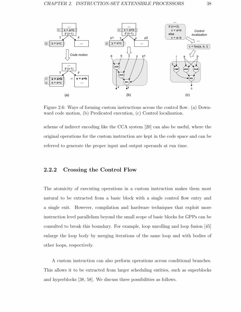
CHAPTER 2. INSTRUCTION-SET EXTENSIBLE PROCESSORS 38
(a)
…
…s = a+bif (i>1)
s = s+c
T F
s = a+b…
…if (i>1)
s = a+bs = s+c
T F
Code motion
i1:
i2:
i1:
i2:
i1’:
(c)(b)
ADD
SEL
ba p1
y
ADD
c
x
y
…
…x = a+bif (i>1)
y = x+c
p1 p2T F
i1:
i2:
if (i==2)c = a+b
elsec = a–b
c = foo(a, b, i)
…
…
Controllocalization
ADD SUB
SEL
CMP
a bi
2
c
Figure 2.6: Ways of forming custom instructions across the control flow. (a) Down-ward code motion, (b) Predicated execution, (c) Control localization.
scheme of indirect encoding like the CCA system [20] can also be useful, where the
original operations for the custom instruction are kept in the code space and can be
referred to generate the proper input and output operands at run time.
2.2.2 Crossing the Control Flow
The atomicity of executing operations in a custom instruction makes them most
natural to be extracted from a basic block with a single control flow entry and
a single exit. However, compilation and hardware techniques that exploit more
instruction level parallelism beyond the small scope of basic blocks for GPPs can be
consulted to break this boundary. For example, loop unrolling and loop fusion [45]
enlarge the loop body by merging iterations of the same loop and with bodies of
other loops, respectively.
A custom instruction can also perform operations across conditional branches.
This allows it to be extracted from larger scheduling entities, such as superblocks
and hyperblocks [38, 58]. We discuss three possibilities as follows.

CHAPTER 2. INSTRUCTION-SET EXTENSIBLE PROCESSORS 39
First, code motion techniques can be used to move operations of the custom
instruction originally spanning across the conditional branch together in a single
basic block. The correctness of the program is preserved by adding compensation
code and/or instruction reordering within the basic block and surrounding ones.
This process is essentially the same as the bookkeeping code induced through code
motion used in trace scheduling [27]. An example of a custom instruction identified
across a conditional branch consisting of two operations i1 and i2 is shown in
Figure 2.6(a). In this example, we move operation i1 originally before the branch
downwards to the taken side, where operation i2 resides. Here, the branch condition
must not be dependent on the moving operation (i1). If any operation on the other
side of the branch depends directly or indirectly on the result of the moving operation
(variable s), the moving operation must be duplicated there (i1’) to maintain the
semantic correctness of the program. After code motion, the custom instruction will
be able to safely replace operations i1 and i2.
Second, given architectural support, predicated execution can be exploited to
handle operations across conditional branches. In predicated execution, the execu-
tion of an instruction is data-dependent on an extra boolean operand, referred to as
the predicate, determined by the outcome of the branch condition. If the predicate
of the instruction is true, it is executed normally; otherwise, it will be “squashed”
by being converted to a no op before entering the execution stage of the pipeline.
By using predicates, the original control dependence is converted to data depen-
dencies, and the conditional branch is eliminated [36]. This conversion process is
called “if-conversion”. For a custom instruction, each predicate of the constituent
operations is an extra input to a selector (multiplexor). All the included operations
are executed, and the correct results are selected to output. Figure 2.6(b) shows
an example. After if-conversion, the code is merged into a single big basic block,
with operations on the two sides of the original branch associated with predicate p1

CHAPTER 2. INSTRUCTION-SET EXTENSIBLE PROCESSORS 40
and p2 respectively (p2 = p1). The lower part of the figure shows the logic of the
custom instruction consisting of operation i1 and i2. Note that even though y is
a destination operand in operation i2, it is still required as an input, because its
original value is needed if predicate p1 is not true5. Unlike code motion, a custom
instruction using predicates can include operations on both sides of the conditional
branch.
Third, control localization transforms the entire branch into a temporary, ag-
gregate function [54]. This function can be implemented as a custom instruction in
a similar way to that of predicated execution (execute both branches and select the
correct output). It also can be treated as a single unit that can be further combined
with other operations. Figure 2.6(c) shows an example of control localization.
5However, this input can be eliminated if certain mechanism is devised not to overwrite y if itsvalue does not need to be changed (depending on the value of the predicate).
Chapter 3
Related Works
As people are walking all the time, in the same spot, a path appears.
– Lu Xun, in “Village Opera”
Identifying the set of custom instructions for the given application is the hardware-
software partitioning problem that divides the computation between the processor
execution (by base instructions) and hardware execution (by custom instructions).
The goal of this process is to find a relatively small set of patterns from the appli-
cation for custom instructions so as to meet design objectives (e.g., performance,
energy improvement). It further involves the following two subproblems. (1) Candi-
date pattern enumeration, which enumerates suitable patterns from the application
as potential candidates for custom instructions. (2) Custom instruction selection,
which selects an optimal subset of the patterns as custom instructions under various
design constraint. A large body of research has been devoted into custom instruction
identification. We review the related works in this chapter.
41

CHAPTER 3. RELATED WORKS 42
3.1 Candidate Pattern Enumeration
Some early works generates candidate complex instructions directly on the linear
code space by iteratively combining operations in subsequent lines of code [10]. It
is restrictive, since the linear layout of the code sequence reflects only one possible
partial order of the operations from the exact dependencies among them. Instead,
dataflow graph (DFG) is used as a general model across nearly all other works. A
DataFlow Graph G(V,E) represents the computation flow of data corresponding
to a code fragment of the application. The nodes V represent the operations and
the edges E represent the dependencies among the operations. G(V,E) is a directed
acyclic graph (DAG). Given a DFG, a pattern is an induced subgraph of the DFG.
A pattern can be a possible candidate for custom instruction. The candidate pattern
enumeration problem is to enumerate subgraphs suitable for custom instructions.
The number of patterns of a DFG is exponential in terms of the number of nodes
of the DFG. Fortunately, not all the patterns are feasible for custom instructions.
For example, a non-convex pattern which involves inter-dependency with operations
outside the pattern is infeasible, because it cannot be executed atomically (e.g.,
pattern {1, 3} consisting of node 1 and 3 in Figure 3.1 is not convex, because an
outside node, node 2, depends on the outcome of node 3, while node 1 depends on the
outcome of node 2). Architectural constraints also impose feasibility requirement on
the number of input/output operands of a pattern. Other constraints may also be
imposed artificially to reduce the complexity of the enumeration. Here, we classify
the previous works in pattern enumeration according to the restrictions imposed on
the feasibility of patterns and properties of the pattern enumeration process.

CHAPTER 3. RELATED WORKS 43
&
+
+&
+
+
|0
1
2
3
4
5
6
&
+
+&
+
+
|0
1
2
3
4
5
6
(a) (b)
+
>>
&+
&
–0
1
3
5
2
4
6
(c)
+
Figure 3.1: Dataflow graph. (a) Two non-overlapped candidate patterns, (b) Over-lapped candidate patterns, (c) Overlapped patterns cannot be scheduled together.
3.1.1 A Classification of Previous Custom Instruction Enu-
meration Methods
Topology Only tree patterns are considered in [57, 73]. The rationale behind
this is that dynamic programming can be applied to cover the DFG (tree) optimally
using as few tree patterns as possible in polynomial time [2]. This simplifies the code
generation process using the pattern matcher. However, as pointed out in [56], trees
are heuristic formulation of the original DFGs, which are DAGs. When the DFG
is not a tree, it will be decomposed into a forrest of disjoint trees. This artificially
breaks some dependent operations in the original DFG apart, and deprives them of
being included in the same pattern. Most other works identify DAG subgraphs for
candidates.
Number of Operands The maximum number of input and output operands of
custom instructions is typically constrained by the length of the instruction and/or
the number of ports to the register files. However, these restrictions can sometime
lead to very efficient enumeration algorithms. For example, Pozzi et al.[67] has
developed a greedy algorithm that can identify the maximal Multiple Inputs Single
Output (MISO) patterns. The complexity of the algorithm is linear in the number of

CHAPTER 3. RELATED WORKS 44
nodes in the DFG. The problem of using Multiple Inputs Multiple Outputs (MIMO)
patterns is that there can potentially be exponential number of them in terms of
the number of nodes in the DFG. Arnold et al. [6] use an iterative technique that
replaces the occurrences of previously identified smaller patterns with single nodes
to avoid the exponential blowup. Cong et al. [25] enumerate all possible K-feasible
cones (a K-feasible cone is a special case of MIMO subgraph which has a single sink
node and at most K input operands.) through a single pass of the DFG. Choi et al.
[19] restrict the number of operations that can be included in a pattern. Clark et al.
[22] use a heuristic algorithm that starts with small MIMO patterns and expands
their patterns only in the directions that can possibly lead to good patterns through
a guiding function. Baleani et al. [9] use another heuristic algorithm that adds
nodes to the current pattern in topological order till input or output constraint is
violated; the algorithm then starts a new pattern only with the node that caused the
violation. All these algorithms only generate a small subset of the candidate patterns
that meet input and output constraints. They may miss opportunities to produce
the globally optimal set of custom instructions. During the course of research in
this thesis, Atasu’s work [8] is the only approach that exhaustively enumerates all
possible patterns. However, scalability becomes a major obstacle when the DFG
size increases. Since we are targeting the same goal, we will describe [8] in detail
later in Section 4.2.1. Later, Chen et. al. propose another algorithm [17] to this
problem, which reports similar run time to that in this thesis.
Connectivity A candidate subgraph (pattern) may contain one or more disjoint
components. Including multiple components in a subgraph increases the potential to
exploit parallelism and thus may provide better performance if the base architecture
does not support instruction-level parallelism (ILP). On the other hand, doing so
may not be beneficial for an ILP processor that would have been able to exploit this
parallelism anyway. In [35] and [37], independent operations which can be scheduled

CHAPTER 3. RELATED WORKS 45
in the same time step form a candidate pattern. [8, 19, 28] consider independent
operations as well as dependent ones within a candidate pattern. Others [6, 9, 22,
25, 67, 57, 73] identify subgraphs with only one component.
Overlap As the final set of selected custom instructions do not normally overlap
in the DFG, some works [9, 67] do not consider overlapped candidate patterns (e.g.,
patterns {0, 1, 2} and {1, 2, 3} overlaps at node 1 and 2, so only one of them will be
enumerated). Enumerating non-overlapping candidate patterns requires only linear
time since each node on the DFG is visited only once. However, isomorphic patterns
embedded inside the DFG may be missed, which yields poor result when the design
constraints are tight. For example in Figure 3.1(a), when only 1 custom instruction
is allowed, pattern {0, 1, 2} may be chosen, ignoring the possibility that {4, 5, 6}
and {1, 2, 3} are isomorphic and can be accelerated by the same custom instruction.
Other works [8, 6, 9, 22, 25] enumerate overlapped patterns as they may be used to
produce a better optima considering custom instruction reuse. Figure 3.1(b) shows
all the 3-input, 1-output convex patterns of the DFG, where isomorphic patterns
are exposed so as to be properly reused.
Implicit pattern enumeration Two recent works [7, 55] use ILP formulation
to generate a single best performing subgraph in each iteration of their algorithms.
In this way, all the subgraphs are potentially enumerated in an implicit manner
and evaluated by the ILP solver. Only the best one is produced. However, in
order for the algorithms to terminate, the constituent nodes in the current best
subgraph cannot be included in further subgraphs, which means candidate subgraphs
generated during the iterations cannot be overlapped. These methods therefore
may miss custom instruction reuse opportunities. All other works identify patterns
explicitly.

CHAPTER 3. RELATED WORKS 46
Order of pattern identification and selection Many previous works take a
two step approach where the first step identifies the set of candidate patterns and
the second step does the selection. Some combine the two steps. For such works like
[7, 22], candidate enumeration step is by itself a screening process that eliminates
patterns unlikely to be selected during the selection step. This reduces the time and
storage complexity of the algorithm at the risk of missing the global optima. In [37],
potential candidate patterns are generated as part of the neighbor states during the
simulated annealing process to produce the best schedule time (with the selection
of complex instructions).
3.2 Custom Instruction Selection
In custom instruction selection, the benefit of a candidate pattern is evaluated as
the product of its speedup cycles (if implemented as a custom instruction) and its
execution frequency via profiling. Each pattern also has a cost value in terms of
silicon area. The process generally aims at selecting a subset from the candidate
patterns under the cost budget for the best performance gain.
Usually, only a subset of the enumerated candidate patterns will be selected for
implementation by custom instructions. There are two reasons behind this. First,
the resource is limited for custom instructions and custom functional units. Adding
many custom instructions for the application does not only cost extra resource (in
terms of silicon area, or reconfiguration time in case of reconfigurable implemen-
tation), but also complicates the circuit design (e.g., decoder, bypass network).
Therefore, only the most cost-effective custom instructions will be selected. Second,
only a subset of patterns will be used to cover the code of the application in code
generation. Usually the code is covered by a non-overlapping set of patterns, such
that a base operation is covered by at most one custom instruction. The potential
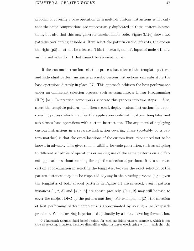
CHAPTER 3. RELATED WORKS 47
problem of covering a base operation with multiple custom instructions is not only
that the same computations are unnecessarily duplicated in these custom instruc-
tions, but also that this may generate unschedulable code. Figure 3.1(c) shows two
patterns overlapping at node 4. If we select the pattern on the left (p1), the one on
the right (p2) must not be selected. This is because, the left input of node 4 is now
an internal value for p1 that cannot be accessed by p2.
If the custom instruction selection process has selected the template patterns
and individual pattern instances precisely, custom instructions can substitute the
base operations directly in place [37]. This approach achieves the best performance
under an omniscient selection process, such as using Integer Linear Programming
(ILP) [51]. In practice, some works separate this process into two steps — first,
select the template patterns, and then second, deploy custom instructions in a code
covering process which matches the application code with pattern templates and
substitutes base operations with custom instructions. The argument of deploying
custom instructions in a separate instruction covering phase (probably by a pat-
tern matcher) is that the exact locations of the custom instructions need not to be
known in advance. This gives some flexibility for code generation, such as adapting
to different schedules of operations or making use of the same patterns on a differ-
ent application without running through the selection algorithms. It also tolerates
certain approximation in selecting the templates, because the exact selection of the
pattern instances may not be respected anyway in the covering process (e.g., given
the templates of both shaded patterns in Figure 3.1 are selected, even if pattern
instances {1, 2, 3} and {4, 5, 6} are chosen precisely, {0, 1, 2} may still be used to
cover the subject DFG by the pattern matcher). For example, in [25], the selection
of best performing pattern templates is approximated by solving a 0-1 knapsack
problem1. While covering is performed optimally by a binate covering formulation.
10-1 knapsack assumes fixed benefit values for each candidate pattern template, which is nottrue as selecting a pattern instance disqualifies other instances overlapping with it, such that the

CHAPTER 3. RELATED WORKS 48
Liem et al. [57] use dynamic programming to select patterns by covering the
subject DFG (tree) with the minimum number of tree patterns (instances). Arnold
[5] modifies the dynamic programming to handle the DAGs instead of just trees.
This is similar to the technology mapping problem in hardware synthesis. However,
the process of dynamic programming is unaware of subgraph isomorphism, that is, it
does not minimize the number of pattern templates and hence custom instructions.
Brisk et al. [11] use All-Pairs Common Slack Graph (APCSG) to capture the
extent of feasibility that two operations may be paired (grouped) together. At each
step, the pairs are evaluated. The value of the same pair type is accumulated so
as to account for isomorphism. The top ranked pairs are merged as single nodes
on both APCSG and the subject DFG at the end of each step. These nodes can
be paired iteratively and grow in the later steps. The algorithm terminates after
a certain coverage of the subject DFG is reached. Other greedy heuristics are also
proposed based on the priority ranking of the candidate patterns [18, 22, 49]. Even
though heuristic methods may miss the global optima, they are very useful as they
often give good enough results typically with quadratic time complexity.
In order to achieve better optima, genetic algorithm (GA) is employed in [73].
A chromosome represents a selection of the patterns. The cross-over between two
feasible chromosomes is ensured to produce a feasible off-spring by removing the con-
flicting patterns (which cover the same base operation). Mutation of a chromosome
is done by adding a random pattern which is not yet included to the chromosome,
and removing the other patterns conflicting with the added one. The fitness function
favors the case where more number of base operations are covered with less number
of pattern templates. The GA terminates after a certain number of generations,
and the result with the best fitness value is used to cover the application. In [65],
GA is extended to optimize performance using run-time reconfigurable CFUs. A
actual benefit values of templates involving those instances need to be updated.
CHAPTER 3. RELATED WORKS 49
Multi-objective GA based method is described in [15] to discover the Pareto front of
the performance improvement under different values of the area constraint instead
of a single solution. Simulated annealing (SA) is used in [37].
Integer linear programming formulation is described in [51] with the objective
to maximize performance under the constraints of chip area and number of custom
instructions. Branch-and-bound algorithm is used in [77]. While guaranteeing the
optimal result, these approaches have exponential run time complexity, and thus
need to be used selectively.
Chapter 4
Scalable Custom Instructions
Identification
More knowledge means less search. – Patrick Henry Winston
Modern compiler techniques such as trace, superblock/hyperblock formation,
and loop unrolling often explore opportunities across basic block boundaries. Dataflow
graphs involving multiple basic blocks can be much larger than those of individual
ones. Moreover, datapath intensive embedded applications (such as encryption al-
gorithms) usually contain huge basic blocks themselves. These large DFGs pack
considerable amount of operations suitable for custom instructions, such that larger
subgraphs involving more operations can be formed for greater performance improve-
ment. It is important that the custom instruction identification algorithm is scalable
enough to explore large DFGs and produce subgraphs under relaxed architectural
constraints. In this chapter, we address the scalability issues of custom instruction
enumeration and describe an efficient algorithm for the exact enumeration of all
possible candidate instructions.
50

CHAPTER 4. SCALABLE CUSTOM INSTRUCTIONS IDENTIFICATION 51
4.1 Custom Instruction Enumeration Problem
Custom instruction identification attempts to find a relatively small set of common
subgraphs from the application’s dataflow graph for custom instructions, so as to
improve the system performance at reasonable hardware cost. Suitable subgraphs
(or patterns) need to be identified first, as candidates for custom instructions among
which the best ones can be selected. Obviously, the effect of the final selection
depends critically on the property of the candidate subgraphs.
Enumerating all possible subgraphs of a given graph is intractable and compu-
tationally expensive. The number of subgraphs or patterns for a DFG is, in general,
exponential in terms of the number of nodes in the DFG. However, some of these
subgraphs are infeasible due to various microarchitectural constraints (e.g., max-
imum number of input and output operands, area, and delay of each subgraph).
Moreover, a subgraph is infeasible if the custom instruction cannot be executed
atomically (named as convexity constraint – see Section 4.1.1 for details).
As we have discussed in Chapter 3, previous approaches either put very limiting
constraints on the number of operands [25, 67] or use heuristics [9, 22] to explore
the design space quickly. However, tight constraints can significantly restrict the
performance potential of using custom instructions. The custom instruction identi-
fication approach proposed in [8] is the only work targeting exhaustive enumeration
of feasible patterns. The algorithm walks through the design space represented by a
binary decision tree, and prunes unnecessary design points effectively based on con-
straint violation of patterns. However, in the worst case, it will look at 2N patterns
where N is the number of nodes in the DFG. Therefore, scalability issues may still
occur when it deals with very large DFGs.
Next, we formally define the custom instruction enumeration problem and no-
tions used in the later part of this chapter.
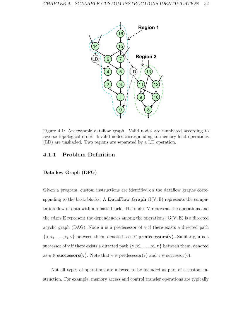
CHAPTER 4. SCALABLE CUSTOM INSTRUCTIONS IDENTIFICATION 52
0
1
3
5
7
15
16
2
4
6LD
14
LD
8
10
12
9
11
13
Region 1
Region 2
Figure 4.1: An example dataflow graph. Valid nodes are numbered according toreverse topological order. Invalid nodes corresponding to memory load operations(LD) are unshaded. Two regions are separated by a LD operation.
4.1.1 Problem Definition
Dataflow Graph (DFG)
Given a program, custom instructions are identified on the dataflow graphs corre-
sponding to the basic blocks. A DataFlow Graph G(V,E) represents the compu-
tation flow of data within a basic block. The nodes V represent the operations and
the edges E represent the dependencies among the operations. G(V,E) is a directed
acyclic graph (DAG). Node u is a predecessor of v if there exists a directed path
{u, x1, . . . , xi, v} between them, denoted as u ∈ predecessors(v). Similarly, u is a
successor of v if there exists a directed path {v, x1, . . . , xi, u} between them, denoted
as u ∈ successors(v). Note that v ∈ predecessor(v) and v ∈ successor(v).
Not all types of operations are allowed to be included as part of a custom in-
struction. For example, memory access and control transfer operations are typically

CHAPTER 4. SCALABLE CUSTOM INSTRUCTIONS IDENTIFICATION 53
not included. Therefore, we mark the nodes of the DFG as valid nodes or invalid
nodes. A node is a valid node if its corresponding operation can be included as
part of a custom instruction; otherwise, it is an invalid node. An example DFG is
shown in Figure 4.1.
A DFG can be partitioned into multiple regions. Given a DFG G(V,E), we
define a region R(V′,E′) as the maximal subgraph of G s.t. (1) V′ contains only
valid nodes, (2) there exists a path between any pair of nodes of V′ in the undirected
graph that underlies R, and (3) there does not exist any edge between a node in V′
and a valid node in (V − V′). Invalid nodes do not belong to any region. Figure 4.1
shows a DFG divided into two regions by a memory load operation.
Patterns
Given a DFG, a pattern is an induced subgraph of the DFG. A pattern can be a
possible candidate for custom instruction. For convenience, we represent a pattern
by its set of nodes. A pattern p is connected if for any pair of nodes 〈u, v〉 in
p, there exists a path between u and v in the undirected graph that underlies the
directed induced subgraph of p. A pattern is disjoint if it is not connected. The
number of input and output operands of p are denoted as IN(p) and OUT(p),
respectively. A node of p connected to an input (output) operand is called an input
(output) node, and we denote p’s input nodes and output nodes as IN SET(p)
and OUT SET(p), respectively. Note that immediate operands are also counted
as input operands. Since isomorphic subgraphs with different immediate values
are exploited with the same custom instruction, the immediate values need to be
explicitly encoded in the instructions.
The following special patterns are of interest for the custom instruction enumer-
ation problem.
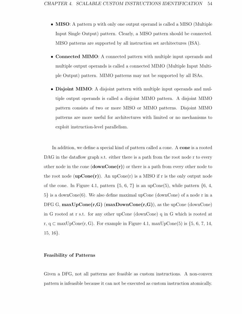
CHAPTER 4. SCALABLE CUSTOM INSTRUCTIONS IDENTIFICATION 54
• MISO: A pattern p with only one output operand is called a MISO (Multiple
Input Single Output) pattern. Clearly, a MISO pattern should be connected.
MISO patterns are supported by all instruction set architectures (ISA).
• Connected MIMO: A connected pattern with multiple input operands and
multiple output operands is called a connected MIMO (Multiple Input Multi-
ple Output) pattern. MIMO patterns may not be supported by all ISAs.
• Disjoint MIMO: A disjoint pattern with multiple input operands and mul-
tiple output operands is called a disjoint MIMO pattern. A disjoint MIMO
pattern consists of two or more MISO or MIMO patterns. Disjoint MIMO
patterns are more useful for architectures with limited or no mechanisms to
exploit instruction-level parallelism.
In addition, we define a special kind of pattern called a cone. A cone is a rooted
DAG in the dataflow graph s.t. either there is a path from the root node r to every
other node in the cone (downCone(r)) or there is a path from every other node to
the root node (upCone(r)). An upCone(r) is a MISO if r is the only output node
of the cone. In Figure 4.1, pattern {5, 6, 7} is an upCone(5), while pattern {6, 4,
5} is a downCone(6). We also define maximal upCone (downCone) of a node r in a
DFG G, maxUpCone(r,G) (maxDownCone(r,G)), as the upCone (downCone)
in G rooted at r s.t. for any other upCone (downCone) q in G which is rooted at
r, q ⊂ maxUpCone(r,G). For example in Figure 4.1, maxUpCone(5) is {5, 6, 7, 14,
15, 16}.
Feasibility of Patterns
Given a DFG, not all patterns are feasible as custom instructions. A non-convex
pattern is infeasible because it can not be executed as custom instruction atomically.
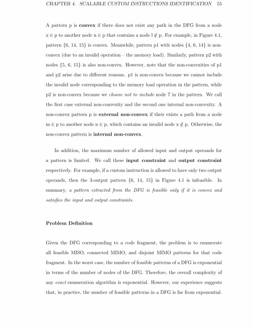
CHAPTER 4. SCALABLE CUSTOM INSTRUCTIONS IDENTIFICATION 55
A pattern p is convex if there does not exist any path in the DFG from a node
x ∈ p to another node n ∈ p that contains a node l /∈ p. For example, in Figure 4.1,
pattern {6, 14, 15} is convex. Meanwhile, pattern p1 with nodes {4, 6, 14} is non-
convex (due to an invalid operation – the memory load). Similarly, pattern p2 with
nodes {5, 6, 15} is also non-convex. However, note that the non-convexities of p1
and p2 arise due to different reasons. p1 is non-convex because we cannot include
the invalid node corresponding to the memory load operation in the pattern, while
p2 is non-convex because we choose not to include node 7 in the pattern. We call
the first case external non-convexity and the second one internal non-convexity. A
non-convex pattern p is external non-convex if their exists a path from a node
m ∈ p to another node n ∈ p, which contains an invalid node x /∈ p. Otherwise, the
non-convex pattern is internal non-convex.
In addition, the maximum number of allowed input and output operands for
a pattern is limited. We call these input constraint and output constraint
respectively. For example, if a custom instruction is allowed to have only two output
operands, then the 3-output pattern {6, 14, 15} in Figure 4.1 is infeasible. In
summary, a pattern extracted from the DFG is feasible only if it is convex and
satisfies the input and output constraints.
Problem Definition
Given the DFG corresponding to a code fragment, the problem is to enumerate
all feasible MISO, connected MIMO, and disjoint MIMO patterns for that code
fragment. In the worst case, the number of feasible patterns of a DFG is exponential
in terms of the number of nodes of the DFG. Therefore, the overall complexity of
any exact enumeration algorithm is exponential. However, our experience suggests
that, in practice, the number of feasible patterns in a DFG is far from exponential.

CHAPTER 4. SCALABLE CUSTOM INSTRUCTIONS IDENTIFICATION 56
Therefore, it is possible to design an efficient algorithm for exact enumeration of
feasible patterns.
4.2 Exhaustive Pattern Enumeration
During the course of the work in this thesis, method in [8, 66] is the only previous
approach that exhaustively enumerates all feasible patterns of a DFG1. We call this
the SingleStep algorithm as it enumerates all feasible MISO, connected MIMO, and
disjoint MIMO patterns through a combined design space exploration. In contrast,
we call our algorithm MultiStep algorithm as it generates MISO, connected MIMO,
and disjoint MIMO patterns in three different stages. We first describe SingleStep
algorithm in this section, followed by our own algorithm.
4.2.1 SingleStep Algorithm
The SingleStep algorithm first assigns labels 0 . . .N− 1 to the valid operations
(nodes) of the DFG in reverse topological order, where N is the number of valid
operations in the DFG. It then searches an abstract binary tree containing N + 1
levels and 2N+1 − 1 nodes to generate feasible patterns. The root node at level 0
represents the empty pattern. The two children of the root represent the presence
and absence of operation 0, i.e., an empty pattern and a pattern containing opera-
tion 0, respectively. The nodes at level i (0 < i ≤ N) represent all possible patterns
with operations 0 . . . i− 1. Basically, the search tree visits the operations in reverse
topological order and explores the patterns corresponding to presence/absence of
each operation. Clearly, the search space is exponential. However, the algorithm
1[66] describes an improved version of the algorithm in [8] by the same authors. We use [66] asthe baseline for efficiency comparison.

CHAPTER 4. SCALABLE CUSTOM INSTRUCTIONS IDENTIFICATION 57
uses a clever strategy to prune the search space. If the pattern corresponding to
a node s in the abstract search tree violates output and/or convexity constraint,
then there is no need to explore the subtree of s. As the operations in the DFG are
visited in reverse topological order, all the patterns corresponding to the nodes in
the subtree of s are guaranteed to violate output and/or convexity constraint. Due
to the same reasoning, certain cases of input violation caused by permanent inputs,
which once introduced cannot be resolved in the deeper subtree, can also be used
to prune the search space.
4.2.2 MultiStep Algorithm
In contrast to the SingleStep algorithm, our MultiStep algorithm does not attempt
to generate all feasible patterns in a single step. It breaks up the pattern generation
process into three steps corresponding to cone, connected MIMO, and disjoint MIMO
patterns. The first step generates upCones and downCones. Recall that a MISO
pattern is a downCone with only one output node. Therefore, the first step implicitly
generates all the MISO patterns. The second step combines two or more cones to
generate connected MIMO patterns, and finally the third step combines two or more
cones/MIMO patterns to generate disjoint MIMO patterns.
The MultiStep algorithm is based on the intuition that it is advantageous to
separate out connected and disjoint MIMO pattern generation. The reason is the
following. On one hand, connected MIMO pattern generation algorithm does not
need to consider nodes that are far apart and have no chance of participating in a
connected pattern together. Therefore the design space is reduced considerably. On
the other hand, lots of infeasible patterns are filtered out during connected pattern
generation step and are not considered subsequently during disjoint pattern gener-
ation step. Thus the separation of concern speeds up the algorithm substantially.

CHAPTER 4. SCALABLE CUSTOM INSTRUCTIONS IDENTIFICATION 58
Our enumeration algorithm is supported by the following two theorems.
Theorem 1 Any connected MIMO pattern p with IN(p) input operands and OUT(p)
output operands can be generated by combining convex upCones with at most IN(p)
input operands or convex downCones with at most OUT(p) output operands.
Proof Let v1, . . . , vN be the nodes of p, where N is the number of nodes in p. Clearly,
maxCone(v1, p) ∪ . . .∪ maxCone(vN, p) = p, where maxCone(vi, p) can either be
maxUpCone(vi, p) or maxDownCone(vi, p). First, we prove that for pi = maxUpCone(vi, p),
IN(pi) ≤ IN(p) for any 1 ≤ i ≤ N by showing that any input operand of pi should
also be an input operand of p. We prove this by contradiction. Let us assume the
input operand of pi is not an input to p, it must be produced by a node v such that
v /∈ pi and v ∈ p. However, if such v exists, then v ∈ maxDownCone(vi, p), which
is a contradiction since pi = maxUpCone(vi, p). Second, we prove by contradiction
that pi is convex. Let us assume that pi is non-convex. Then, there exists at least
a pair of nodes m, n ∈ pi such that there exists a path from m to n that contains a
node y /∈ pi. As pi is the maxUpCone of node vi in p, if y /∈ pi, then y /∈ p. There-
fore, p is also non-convex, which is a contradiction. Similarly, we can prove the case
for downCones through the use of maxDownCone(vi, p). �
In other words, it is possible to generate any feasible connected MIMO patterns
by combining one or more cones. For example, the pattern {6, 7, 14, 15} in Fig-
ure 4.1 can be generated by combining upCone(6) = {6, 14, 15} with downCone(15)
= {7, 15}. The above theorem provides a key search space reduction technique by
excluding some combination of cones. Specifically, to generate all the connected
MIMO patterns, MultiStep algorithm only needs all upCones that satisfy convex-
ity/input constraints and all downCones that satisfy convexity/output constraints.
This allows the algorithm to prune aggressively.

CHAPTER 4. SCALABLE CUSTOM INSTRUCTIONS IDENTIFICATION 59
Theorem 2 Any connected component pi of a feasible disjoint pattern dp must be
a feasible connected pattern.
Proof A connected component pi of a disjoint MIMO pattern dp is a maximal
connected subgraph in dp. An input of pi must also be an input of dp. So
IN(pi) ≤ IN(dp). As dp satisfies input constraint, pi must also satisfy the input
constraint. The same reasoning holds for the output constraint.
We prove by contradiction that pi is convex. Let us assume pi is non-convex.
Then there exists at least a pair of nodes m, n ∈ pi s.t. there exists a path from m
to n that contains a node x /∈ pi. There are two cases for x. (1) x /∈ dp: In this
case dp is also non-convex, which is a contradiction; (2) x ∈ dp: As pi is a maximal
connected subgraph, x is not connected to pi. So there must be two nodes y, z /∈ pi
and connected to pi on a path 〈m, y, . . . , x, . . . , z, n〉. We have y, z /∈ dp, otherwise
they will belong to pi too. So now we have two paths 〈m, y, . . . , x〉 and 〈x, . . . , z, n〉
that make dp non-convex, which is again a contradiction. So pi must be convex. �
Theorem 2 shows that a feasible disjoint pattern can be generated from one or
more feasible connected patterns. The possible combination of feasible patterns is
much smaller than that of arbitrary patterns, resulting in more efficient enumeration.
The rest of this section describes our MultiStep algorithm in detail.
4.2.3 Generation of Cones
The first step generates all the convex upCones that satisfy input constraints and
convex downCones that satisfy output constraints. Recall that a cone is a connected
pattern and hence cannot contain nodes from different regions of a DFG. Therefore,
we generate cones for each region individually. First, we traverse the nodes of each

CHAPTER 4. SCALABLE CUSTOM INSTRUCTIONS IDENTIFICATION 60
Algorithm 1: Enumeration of upCones of region RConeGen
beginfor all nodes v of R in topological order do1
upConeSet(v) := {{v}};2
for all possible combination of immediate predecessors of v do3
Let v1, . . . , vi be the selected immediate predecessors;4
tmpConeSet := CrossProduct(upConeSet(v1), . . . , upConeSet(vi), {{v}});5
prune tmpConeSet for convexity and input violation;6
upConeSet(v) := upConeSet(v) ∪ tmpConeSet;7
end
CrossProduct (set1, . . . , setn)begin
resSet := φ;8
set := set1 × . . .× setn;9
for each s ∈ set do10
Let s = 〈s1, . . . , sn〉;11
resSet := resSet ∪ {s1 ∪ . . . ∪ sn};12
return resSet;13
end
region in topological order and calculate the set of possible convex upCones that
satisfy input constraints at each node. Similarly, we traverse the nodes of each
region in reverse topological order to calculate the set of possible convex downCones
at each node that satisfy output constraints.
Algorithm 1 details the generation of upCones for a region R. We define
upConeSet(v) as the set of upCones for node v satisfying both the input operands
and convexity constraints. Recall that each upCone (pattern) in the set upConeSet(v),
in turn, is again represented as a set of nodes. Given a node v, let v1, . . . , vk be its
immediate predecessors in the region. As we are traversing the nodes in topologi-
cally sorted order, the set of upConeSet(vi) (vi ∈ predecessors(v)) is known when v is
visited. Therefore, we can compute upConeSet(v). For example, the upConeSet(14)
and upConeSet(15) (in Figure 4.1) are {{14}} and {{15}, {15, 16}}, respectively.
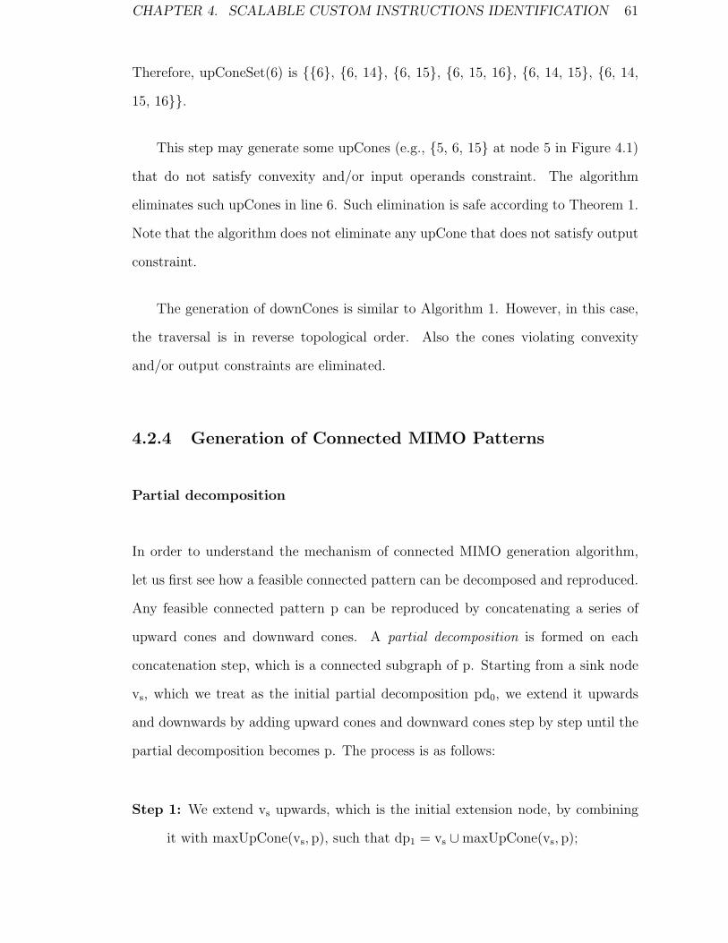
CHAPTER 4. SCALABLE CUSTOM INSTRUCTIONS IDENTIFICATION 61
Therefore, upConeSet(6) is {{6}, {6, 14}, {6, 15}, {6, 15, 16}, {6, 14, 15}, {6, 14,
15, 16}}.
This step may generate some upCones (e.g., {5, 6, 15} at node 5 in Figure 4.1)
that do not satisfy convexity and/or input operands constraint. The algorithm
eliminates such upCones in line 6. Such elimination is safe according to Theorem 1.
Note that the algorithm does not eliminate any upCone that does not satisfy output
constraint.
The generation of downCones is similar to Algorithm 1. However, in this case,
the traversal is in reverse topological order. Also the cones violating convexity
and/or output constraints are eliminated.
4.2.4 Generation of Connected MIMO Patterns
Partial decomposition
In order to understand the mechanism of connected MIMO generation algorithm,
let us first see how a feasible connected pattern can be decomposed and reproduced.
Any feasible connected pattern p can be reproduced by concatenating a series of
upward cones and downward cones. A partial decomposition is formed on each
concatenation step, which is a connected subgraph of p. Starting from a sink node
vs, which we treat as the initial partial decomposition pd0, we extend it upwards
and downwards by adding upward cones and downward cones step by step until the
partial decomposition becomes p. The process is as follows:
Step 1: We extend vs upwards, which is the initial extension node, by combining
it with maxUpCone(vs, p), such that dp1 = vs ∪maxUpCone(vs, p);
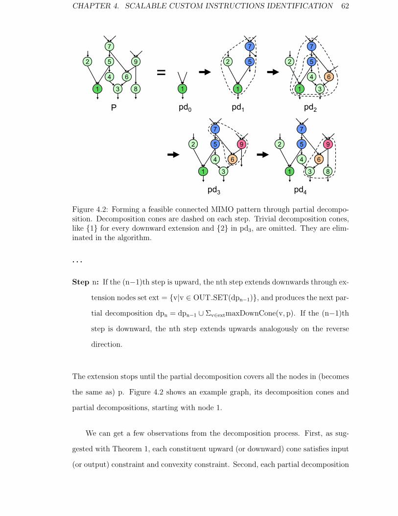
CHAPTER 4. SCALABLE CUSTOM INSTRUCTIONS IDENTIFICATION 62
1
pd0
=5
7
1
2
4
3
6
9
8
P pd1
5
7
1
2 5
7
1
2
4
3
56
pd2
5
7
1
2
4
3
5
9
6
pd3
5
7
1
2
4
3
5
9
8
6
pd4
Figure 4.2: Forming a feasible connected MIMO pattern through partial decompo-sition. Decomposition cones are dashed on each step. Trivial decomposition cones,like {1} for every downward extension and {2} in pd3, are omitted. They are elim-inated in the algorithm.
. . .
Step n: If the (n−1)th step is upward, the nth step extends downwards through ex-
tension nodes set ext = {v|v ∈ OUT SET(dpn−1)}, and produces the next par-
tial decomposition dpn = dpn−1 ∪ Σv∈extmaxDownCone(v, p). If the (n−1)th
step is downward, the nth step extends upwards analogously on the reverse
direction.
The extension stops until the partial decomposition covers all the nodes in (becomes
the same as) p. Figure 4.2 shows an example graph, its decomposition cones and
partial decompositions, starting with node 1.
We can get a few observations from the decomposition process. First, as sug-
gested with Theorem 1, each constituent upward (or downward) cone satisfies input
(or output) constraint and convexity constraint. Second, each partial decomposition
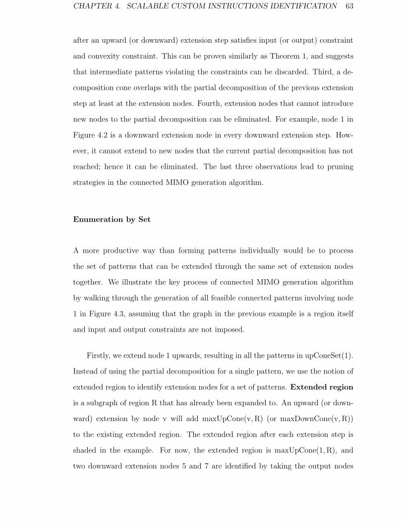
CHAPTER 4. SCALABLE CUSTOM INSTRUCTIONS IDENTIFICATION 63
after an upward (or downward) extension step satisfies input (or output) constraint
and convexity constraint. This can be proven similarly as Theorem 1, and suggests
that intermediate patterns violating the constraints can be discarded. Third, a de-
composition cone overlaps with the partial decomposition of the previous extension
step at least at the extension nodes. Fourth, extension nodes that cannot introduce
new nodes to the partial decomposition can be eliminated. For example, node 1 in
Figure 4.2 is a downward extension node in every downward extension step. How-
ever, it cannot extend to new nodes that the current partial decomposition has not
reached; hence it can be eliminated. The last three observations lead to pruning
strategies in the connected MIMO generation algorithm.
Enumeration by Set
A more productive way than forming patterns individually would be to process
the set of patterns that can be extended through the same set of extension nodes
together. We illustrate the key process of connected MIMO generation algorithm
by walking through the generation of all feasible connected patterns involving node
1 in Figure 4.3, assuming that the graph in the previous example is a region itself
and input and output constraints are not imposed.
Firstly, we extend node 1 upwards, resulting in all the patterns in upConeSet(1).
Instead of using the partial decomposition for a single pattern, we use the notion of
extended region to identify extension nodes for a set of patterns. Extended region
is a subgraph of region R that has already been expanded to. An upward (or down-
ward) extension by node v will add maxUpCone(v,R) (or maxDownCone(v,R))
to the existing extended region. The extended region after each extension step is
shaded in the example. For now, the extended region is maxUpCone(1,R), and
two downward extension nodes 5 and 7 are identified by taking the output nodes

CHAPTER 4. SCALABLE CUSTOM INSTRUCTIONS IDENTIFICATION 64
Extend ({5,7}, down){7}
Node 1, OUT_SET(maxUpCone(1))={5,7}
{5} {5,7}
Extend ({3}, up) Extend ({6}, up){3} {6}
Eliminated
Collect patternsinvolving 1
Collect patternsinvolving 1,5
Collect patternsinvolving 1,5,7
Extend ({9}, down){9}
Extend ({9}, down){9}
Collect patternsinvolving 1,3,5
Collect patternsinvolving 1,5,6,7
Collect patternsinvolving 1,3,5,9
Collect patternsinvolving 1,5,6,7,9
(b) (c) (d)
(e) (f) (g)
Extendedregion
New sub-regionintroduced
{5,7}
{5}
{3}
{6}
{9}
{9}
5
7
1
2
4
3
6
9
8
P
exten
d
extend
5
7
1
2
4
3
6
9
8
(a)
5
7
1
2
4
3
6
9
8
5
7
1
2
4
3
6
9
8
5
7
1
2
4
3
6
9
8
5
7
1
2
4
3
6
9
8
5
7
1
2
4
3
6
9
8
5
7
1
2
4
3
6
9
8
Figure 4.3: Generating all feasible connected patterns involving node 1.
Extend ({5,7}, down)
Node 1, OUT_SET(maxUpCone(1))={5,7}Collect patternsinvolving 1
{7} {5} {5,7}
Extend ({3}, up) Extend ({6}, up)
Eliminated Collect patternsinvolving 1,5
Collect patternsinvolving 1,5,7
5
7
2 9
{3} {6}
Extend ({9}, down){9}
Extend ({9}, down){9}
Collect patternsinvolving 1,3,5
Collect patternsinvolving 1,5,6,71
4
3
6
8
P {9} {9}Collect patternsinvolving 1,3,5,9
Collect patternsinvolving 1,5,6,7,9
E t d d
P
5
7
2
4 6
9 5
7
2
4 6
9 5
7
2
4 6
9
Extendedregion
New sub-regionintroduced
{3} {9}
5
7
2 9
1 3 8 1 3 8 1 3 8
(b) (c) (d){5}
1
4
3
6
8 5
7
2
4 6
9 5
7
2
4 6
9 5
7
2
4 6
9
( )
{5,7}
{6} {9}
1
4
3
6
8 1
4
3
6
8 1
4
3
6
8
(a)
(e) (f) (g)
Figure 4.4: A recursive process of collecting patterns for the example in Fig. 4.3.
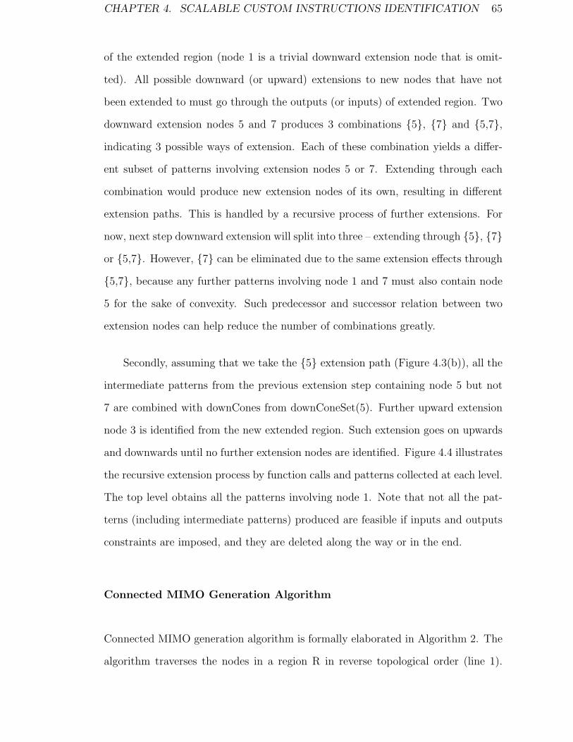
CHAPTER 4. SCALABLE CUSTOM INSTRUCTIONS IDENTIFICATION 65
of the extended region (node 1 is a trivial downward extension node that is omit-
ted). All possible downward (or upward) extensions to new nodes that have not
been extended to must go through the outputs (or inputs) of extended region. Two
downward extension nodes 5 and 7 produces 3 combinations {5}, {7} and {5,7},
indicating 3 possible ways of extension. Each of these combination yields a differ-
ent subset of patterns involving extension nodes 5 or 7. Extending through each
combination would produce new extension nodes of its own, resulting in different
extension paths. This is handled by a recursive process of further extensions. For
now, next step downward extension will split into three – extending through {5}, {7}
or {5,7}. However, {7} can be eliminated due to the same extension effects through
{5,7}, because any further patterns involving node 1 and 7 must also contain node
5 for the sake of convexity. Such predecessor and successor relation between two
extension nodes can help reduce the number of combinations greatly.
Secondly, assuming that we take the {5} extension path (Figure 4.3(b)), all the
intermediate patterns from the previous extension step containing node 5 but not
7 are combined with downCones from downConeSet(5). Further upward extension
node 3 is identified from the new extended region. Such extension goes on upwards
and downwards until no further extension nodes are identified. Figure 4.4 illustrates
the recursive extension process by function calls and patterns collected at each level.
The top level obtains all the patterns involving node 1. Note that not all the pat-
terns (including intermediate patterns) produced are feasible if inputs and outputs
constraints are imposed, and they are deleted along the way or in the end.
Connected MIMO Generation Algorithm
Connected MIMO generation algorithm is formally elaborated in Algorithm 2. The
algorithm traverses the nodes in a region R in reverse topological order (line 1).
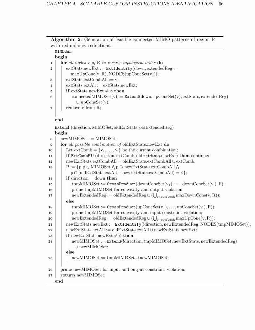
CHAPTER 4. SCALABLE CUSTOM INSTRUCTIONS IDENTIFICATION 66
Algorithm 2: Generation of feasible connected MIMO patterns of region Rwith redundancy reductions.MIMOGenbegin
for all nodes v of R in reverse topological order do1
extStats.newExt := ExtIdentify(down, extendedReg :=2
maxUpCone(v,R),NODES(upConeSet(v)));extStats.extCombAll := v;3
extStats.extAll := extStats.newExt;4
if extStats.newExt 6= φ then5
connectedMIMOSet(v) := Extend(down,upConeSet(v), extStats, extendedReg)6
∪ upConeSet(v);remove v from R;7
end
Extend (direction,MIMOSet, oldExtStats, oldExtendedReg)begin
newMIMOSet := MIMOSet;8
for all possible combination of oldExtStats.newExt do9
Let extComb = {v1, . . . , vi} be the current combination;10
if ExtCombEli(direction, extComb, oldExtStats.newExt) then continue;11
newExtStats.extCombAll = oldExtStats.extCombAll ∪ extComb;12
P := {p|p ∈ MIMOSet∧
p ⊇ newExtStats.extCombAll∧
13
p ∩ (oldExtStats.extAll− newExtStats.extCombAll) = φ};if direction = down then14
tmpMIMOSet := CrossProduct(downConeSet(v1), . . . ,downConeSet(vi),P);15
prune tmpMIMOSet for convexity and output violation;16
newExtendedReg := oldExtendedReg ∪ (⋃
v∈extComb maxDownCone(v,R));17
elsetmpMIMOSet := CrossProduct(upConeSet(v1), . . . ,upConeSet(vi),P));18
prune tmpMIMOSet for convexity and input constraint violation;19
newExtendedReg := oldExtendedReg ∪ (⋃
v∈extComb maxUpCone(v,R));20
newExtStats.newExt := ExtIdentify(!direction,newExtendedReg,NODES(tmpMIMOSet));21
newExtStats.extAll := oldExtStats.extAll ∪ newExtStats.newExt;22
if newExtStats.newExt 6= φ then23
newMIMOSet := Extend(!direction, tmpMIMOSet, newExtStats,newExtendedReg)24
∪ newMIMOSet;else
newMIMOSet := tmpMIMOSet ∪ newMIMOSet;25
prune newMIMOSet for input and output constraint violation;26
return newMIMOSet;27
end

CHAPTER 4. SCALABLE CUSTOM INSTRUCTIONS IDENTIFICATION 67
Algorithm 3: Auxiliary functions for the connected MIMO generation algo-rithm.ExtIdentify (direction, extendedReg, wetReg)begin
/* Identify downward extension nodes */
if direction = down then1
newExt := OUT SET(extendedReg);2
for v ∈ newExt do3
if maxDownCone(v,R) ⊆ extendedReg then remove v from4
newExt;else if v /∈ wetReg then remove v from newExt;5
else// Upward case is analogous.6
return newExt;7
end
bool ExtCombEli (direction, extComb, newExt)begin
for any pair u and v ∈ newExt, where u ∈ predecessor(v) do8
if direction = down∧
u ∈ extComb∧
v /∈ extComb then return true;9
else if direction = up∧
v ∈ extComb∧
u /∈ extComb then return10
true;return false;11
end
It maintains the following invariant: when the traversal of a node v is completed,
all the feasible connected patterns involving v have been enumerated. Therefore,
node v need not be considered further and can be masked, along with existing
subgraphs/cones involving v.
For each starting node v as the initial extension node, which must be a sink
node for the rest of region R, the algorithm resembles the process in the example
of Figure 4.3. It identifies new extension nodes (line 2, 21) and enumerates their
combinations (line 9) upwards and downwards, and splits the search recursively
along each extension node combination with the Extend function. Extend takes in
four arguments: (1) direction can take values up or down, and indicates whether
the current extension step is upward or downward. (2) MIMOSet is a set of patterns

CHAPTER 4. SCALABLE CUSTOM INSTRUCTIONS IDENTIFICATION 68
passed from the previous level, as the base set of patterns to be combined with
cones of extension nodes. (3) oldExtStats contains three sets of extension nodes,
expressing the progress of the extension: newExt is the set of new extension nodes
identified from the previous level, combinations of which will be enumerated and
extended at the current level; extAll is the set of all the extension nodes identified
so far along the recursive extension up to the current level; extCombAll is the set
of all the extension nodes that have actually been extended up to the previous
level. For example, at the bottom level of the middle path (in the dashed box) in
Figure 4.4, node 9 is the only extension node identified from the previous level, so
newExt={9}; extAll={1, 5, 7, 3, 9} and extCombAll={1, 5, 3}. For each extension
node combination (only {9} in this case), the new extCombAll is generated (line
12), and used together with extAll to pick up a subset of patterns in MIMOSet to
extend (line 13). (4) oldExtendedReg is the extended region from the previous step
used to identify further extension nodes (line 2, 21).
Extension nodes are identified in the ExtIdentify function depicted in Algo-
rithm 3. Possible downward extension nodes are identified as the output nodes of
extended region. However, extension nodes that can not produce new patterns are
eliminated in two ways. First, extension nodes that introduce no new extended
region are eliminated (line 4). Second, extension nodes falling outside the wet re-
gion are eliminated (line 5). Wet region (as computed in line 21 of Algorithm 2)
is a subregion of R that contains nodes appearing in at least one subgraph pro-
duced in the current extension step (tmpMIMOSet). These subgraphs are the base
set to be further extended. If none of these subgraphs covers the extension node,
the extension node can be eliminated (recall that a partial decomposition must be
overlapping with the decomposition cone at least on the extension node so as to be
extended). For instance, in the example of Figure 4.3(a), if a 2-input constraint is
imposed, then upConeSet(1) = {{1}, {1, 2}, {1, 5}, {1, 2, 5}}. Extension node 7 will

CHAPTER 4. SCALABLE CUSTOM INSTRUCTIONS IDENTIFICATION 69
be eliminated since it is not covered by the wet region {1, 2, 5}. In other words,
if we see the extended region as the area that have been explored in sight, the wet
region will be the footsteps.
Function ExtCombEli tests a given extension node combination and bypasses it
if it is redundant (line 11 in Algorithm 2). For two downward extension nodes u and
v identified, if u ∈ predecessor(v), the extension node combination with u but not
v has the same effects with the combination containing both, thus can be bypassed
safely (line 9). The reasoning for this is partial decompositions with node u must
also contain node v, thus further extensions of two cases will be the same. Suppose
previous upward extension node e is successor of both u and v (such e must exist
obviously). All the partial decompositions contain node e. As a result, if a partial
decomposition contains u, it must also contain v to ensure the convexity to node e.
Line 10 is the test along upward direction analogously.
4.2.5 Generation of Disjoint MIMO Patterns
Disjoint pattern enumeration algorithm produces the set of all feasible disjoint
MIMO patterns denoted as DPS. According to Theorem 2, each disjoint pattern
dp ∈ DPS is composed of more than one connected patterns that satisfy the input,
output and convexity constraints. We use the the set of all feasible connected MIMO
patterns denoted as CPS as the base to produce all the disjoint patterns.
We observed that the number of output nodes of any feasible disjoint pattern
is simply the summation of those of its constituent connected patterns. Based on
this observation, we classify the patterns according to the the number of output
nodes. We define CPSi and DPSi as the set of all the feasible connected patterns
and disjoint patterns with exactly i output nodes, respectively. Note that according
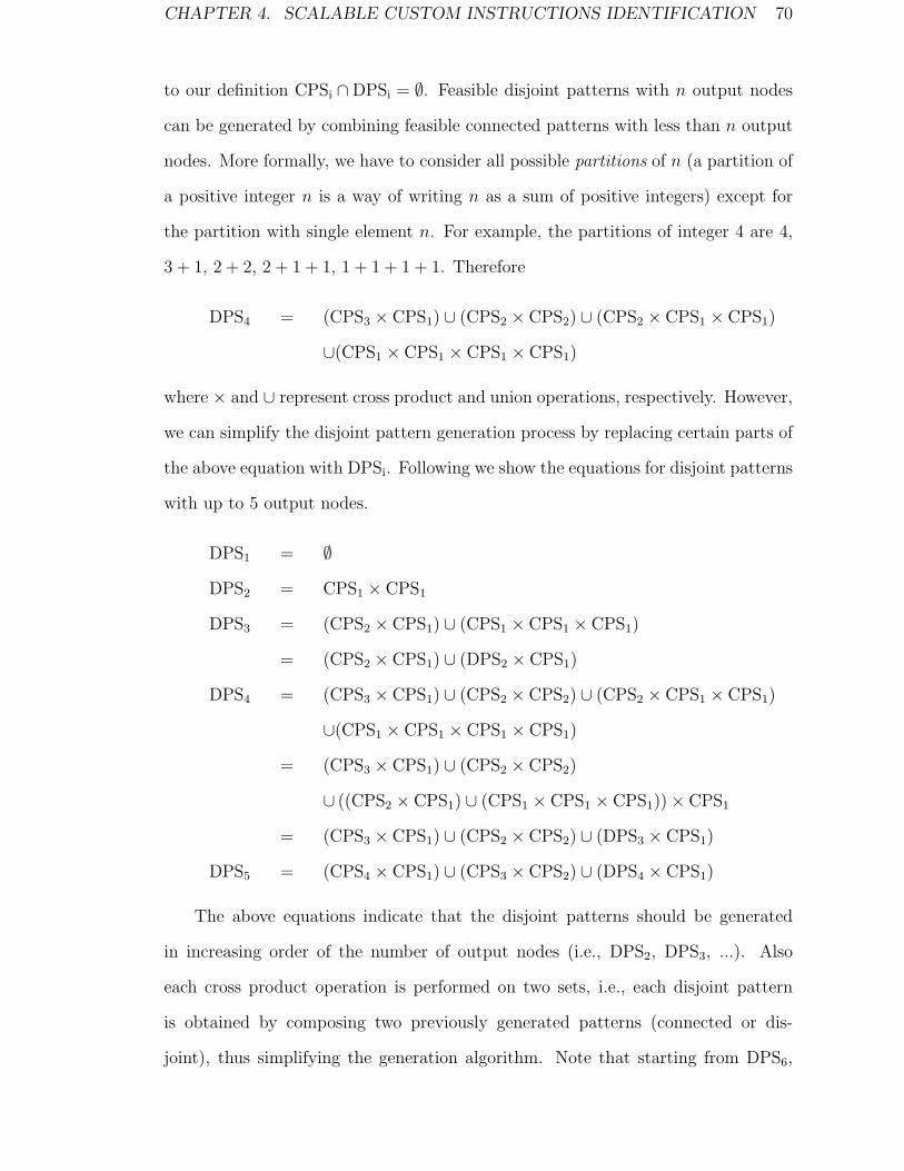
CHAPTER 4. SCALABLE CUSTOM INSTRUCTIONS IDENTIFICATION 70
to our definition CPSi ∩DPSi = ∅. Feasible disjoint patterns with n output nodes
can be generated by combining feasible connected patterns with less than n output
nodes. More formally, we have to consider all possible partitions of n (a partition of
a positive integer n is a way of writing n as a sum of positive integers) except for
the partition with single element n. For example, the partitions of integer 4 are 4,
3 + 1, 2 + 2, 2 + 1 + 1, 1 + 1 + 1 + 1. Therefore
DPS4 = (CPS3 × CPS1) ∪ (CPS2 × CPS2) ∪ (CPS2 × CPS1 × CPS1)
∪(CPS1 × CPS1 × CPS1 × CPS1)
where × and ∪ represent cross product and union operations, respectively. However,
we can simplify the disjoint pattern generation process by replacing certain parts of
the above equation with DPSi. Following we show the equations for disjoint patterns
with up to 5 output nodes.
DPS1 = ∅
DPS2 = CPS1 × CPS1
DPS3 = (CPS2 × CPS1) ∪ (CPS1 × CPS1 × CPS1)
= (CPS2 × CPS1) ∪ (DPS2 × CPS1)
DPS4 = (CPS3 × CPS1) ∪ (CPS2 × CPS2) ∪ (CPS2 × CPS1 × CPS1)
∪(CPS1 × CPS1 × CPS1 × CPS1)
= (CPS3 × CPS1) ∪ (CPS2 × CPS2)
∪ ((CPS2 × CPS1) ∪ (CPS1 × CPS1 × CPS1))× CPS1
= (CPS3 × CPS1) ∪ (CPS2 × CPS2) ∪ (DPS3 × CPS1)
DPS5 = (CPS4 × CPS1) ∪ (CPS3 × CPS2) ∪ (DPS4 × CPS1)
The above equations indicate that the disjoint patterns should be generated
in increasing order of the number of output nodes (i.e., DPS2, DPS3, ...). Also
each cross product operation is performed on two sets, i.e., each disjoint pattern
is obtained by composing two previously generated patterns (connected or dis-
joint), thus simplifying the generation algorithm. Note that starting from DPS6,
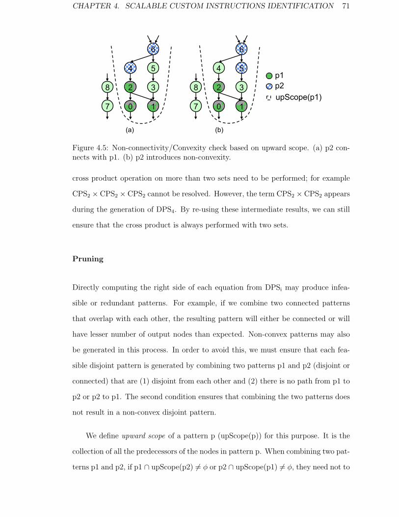
CHAPTER 4. SCALABLE CUSTOM INSTRUCTIONS IDENTIFICATION 71
2
10
(a) (b)
p1
p2
upScope(p1)
4 5
3
6
7
8 2
10
4 5
3
6
7
8
Figure 4.5: Non-connectivity/Convexity check based on upward scope. (a) p2 con-nects with p1. (b) p2 introduces non-convexity.
cross product operation on more than two sets need to be performed; for example
CPS2 × CPS2 × CPS2 cannot be resolved. However, the term CPS2 × CPS2 appears
during the generation of DPS4. By re-using these intermediate results, we can still
ensure that the cross product is always performed with two sets.
Pruning
Directly computing the right side of each equation from DPSi may produce infea-
sible or redundant patterns. For example, if we combine two connected patterns
that overlap with each other, the resulting pattern will either be connected or will
have lesser number of output nodes than expected. Non-convex patterns may also
be generated in this process. In order to avoid this, we must ensure that each fea-
sible disjoint pattern is generated by combining two patterns p1 and p2 (disjoint or
connected) that are (1) disjoint from each other and (2) there is no path from p1 to
p2 or p2 to p1. The second condition ensures that combining the two patterns does
not result in a non-convex disjoint pattern.
We define upward scope of a pattern p (upScope(p)) for this purpose. It is the
collection of all the predecessors of the nodes in pattern p. When combining two pat-
terns p1 and p2, if p1 ∩ upScope(p2) 6= φ or p2 ∩ upScope(p1) 6= φ, they need not to

CHAPTER 4. SCALABLE CUSTOM INSTRUCTIONS IDENTIFICATION 72
be combined because either non-connectivity and/or convexity condition will be vio-
lated. Let us assume that p2 ∩ upScope(p1) 6= φ, there must exists node v ∈ p2 and
u ∈ p1 such that v ∈ predecessors(u). Now that there exists a path 〈v, . . . , xi, . . . , u〉
between v and u, if all xi belongs to either p1 or p2, then the combined subgraph
will be a connected one; otherwise, the combined subgraph should be non-convex.
Figure 4.5 shows these two cases. In disjoint pattern generation process, the upward
scope for each pattern need to be computed and stored to perform this check.
To further prune the search space, we first number the nodes according to reverse
topologically sorted order. Next we define CPSvi as the set of feasible connected
patterns with i output nodes and v as the smallest numbered node. Similar definition
applies to DPSvi . Clearly,
DPSi =⋃
v∈valid nodes
DPSvi
DPS =MAXOUT⋃
i=2
DPSi
where MAXOUT is the output constraint.
Algorithm 4 details the disjoint pattern generation steps. It computes DPSvi for
each valid node v in the innermost loop according to the corresponding equation
(line 8), aggregates them to form DPSi (line 20) and finally DPS (line 21).
DPSvi is computed by combining pattern sets of node v with pattern sets of
node u, where u is bigger than v in reverse topologically sorted order (line 6).
Non-symmetrical terms, such as CPS1 × CPS2 should be combined twice with their
place exchanged (line 18–19). Upward scope check helps reduce the design space
at two places. First, node u can be entirely bypassed if it falls in upScope(v) (line
7); otherwise non-connectivity or convexity will be violated. Second, constituent
pattern p1 from pattern set of v can be bypassed if upScope(p1) overlaps with u
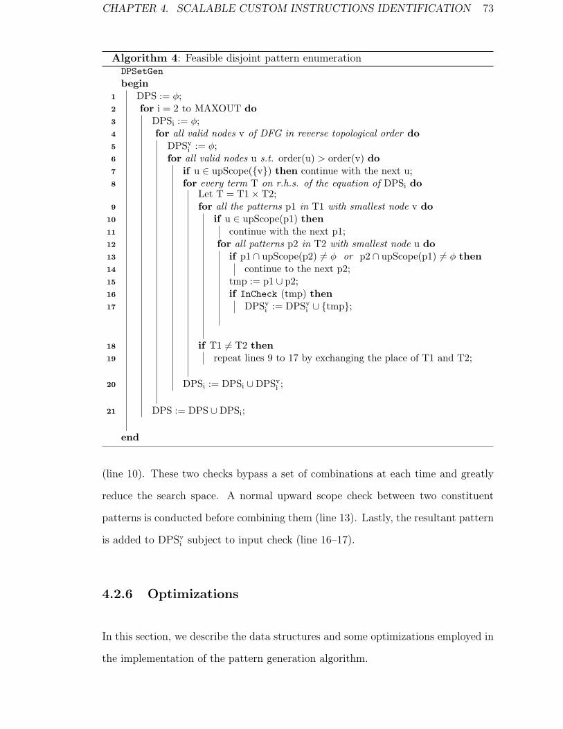
CHAPTER 4. SCALABLE CUSTOM INSTRUCTIONS IDENTIFICATION 73
Algorithm 4: Feasible disjoint pattern enumerationDPSetGenbegin
DPS := φ;1
for i = 2 to MAXOUT do2
DPSi := φ;3
for all valid nodes v of DFG in reverse topological order do4
DPSvi := φ;5
for all valid nodes u s.t. order(u) > order(v) do6
if u ∈ upScope({v}) then continue with the next u;7
for every term T on r.h.s. of the equation of DPSi do8
Let T = T1× T2;for all the patterns p1 in T1 with smallest node v do9
if u ∈ upScope(p1) then10
continue with the next p1;11
for all patterns p2 in T2 with smallest node u do12
if p1 ∩ upScope(p2) 6= φ or p2 ∩ upScope(p1) 6= φ then13
continue to the next p2;14
tmp := p1 ∪ p2;15
if InCheck (tmp) then16
DPSvi := DPSv
i ∪ {tmp};17
if T1 6= T2 then18
repeat lines 9 to 17 by exchanging the place of T1 and T2;19
DPSi := DPSi ∪DPSvi ;20
DPS := DPS ∪DPSi;21
end
(line 10). These two checks bypass a set of combinations at each time and greatly
reduce the search space. A normal upward scope check between two constituent
patterns is conducted before combining them (line 13). Lastly, the resultant pattern
is added to DPSvi subject to input check (line 16–17).
4.2.6 Optimizations
In this section, we describe the data structures and some optimizations employed in
the implementation of the pattern generation algorithm.

CHAPTER 4. SCALABLE CUSTOM INSTRUCTIONS IDENTIFICATION 74
Data structures
We use fixed-length bit vectors to represent each pattern. The length of the bit
vectors is equal to the number of nodes in the DFG. Given the bit vector of a pattern,
each bit simply indicates the presence and absence of a node in that pattern. Bit
vector representation provides a very natural and efficient means to combine two or
more patterns (as in line 12 of Algorithm 1 through bit-wise OR operation). Many
other information related to node set, such as max upward cone, predecessors and
successors of a node, extended region, upward scope of a pattern, are also represented
with bit vectors, and inter-operate efficiently with patterns using bit-wise operations.
We also need to remove duplicates while constructing a set of patterns. This
requires both efficient search as well as insertion that cannot be achieved either with
sorted array or linked list. We maintain a set of patterns as a 2-3 Tree [3]. The
patterns in a 2-3 tree are sorted by the value of their bit-vectors; every query or
insertion of a pattern can be achieved within O(log2(n)) time, where n is the total
number of patterns present in the 2-3 tree. A pattern is inserted in the 2-3 tree only
if it is not present already.
Checking for Input/Output constraints
Given a pattern p generated by combining patterns p1, . . . , pn, IN SET(p)⊆ IN SET(p1)
∪ . . . ∪ IN SET(pn) (similarly for OUT SET(p)). Therefore, in order to check for
violation of input/output operand constraints in a pattern, we will need to look at
the input/output nodes of the constituent patterns. For this purpose, we maintain
the set of input/output nodes with each pattern.

CHAPTER 4. SCALABLE CUSTOM INSTRUCTIONS IDENTIFICATION 75
Checking for convexity constraint
Convexity check of DPSetGen algorithm (Algorithm 4) is done using upward scope
checks because of the peculiarity of non-connectivity. Here we discuss convex-
ity check in ConeGen and MIMOGen algorithms (Algorithm 1 and 2). In order to
check for convexity of a produced pattern p, we consider all immediate succes-
sors from the nodes in OUT SET(p). If, for one such immediate successor u /∈ p,
successors(u) ∩ p 6= φ, then p fails the convexity constraint.
Furthermore, we can use the notion of external non-convexity to prune some
of the participating patterns, including which will definitely cause non-convexity,
before forming new patterns by cross production. This is very helpful in reducing
the intensity of the cross production. Recall that external non-convexity is caused
by invalid nodes. Specifically, for any node v, there exists an external conflicting
set (ECS(v), can be empty) such that any node within cannot coexist with v in
a valid pattern, otherwise external non-convexity will occur. Let us now see the
cross production of ConeGen (as in line 5 of Algorithm 1). As any resultant pattern
contains v, participating patterns from upConeSet(v1), . . . , upConeSet(vi) involving
any node in ECS(v) can be filtered out before the actual cross production. Similarly,
in MIMOGen, because any resultant pattern contains all the selected extension nodes
(newExtStats.extCombAll), participating patterns involving nodes in⋃
viECS(vi)
(vi ∈ newExtStats.extCombAll) should be filtered out before the cross productions
(line 15 and 18).
Computing external conflicting sets involve a pre-processing step. Given a region
R, we first identify special pairs of nodes, called boundary pairs. Two nodes u and
v in R are called a boundary pair if there exists a path 〈u, x1, . . . xn, v〉 in the DFG
s.t. x1, . . . xn do not belong to R. For example in Figure 4.1, 〈4, 14〉 and 〈0, 15〉 are
boundary pairs. Clearly, if 〈u, v〉 is a boundary pair, then u and v cannot coexist
CHAPTER 4. SCALABLE CUSTOM INSTRUCTIONS IDENTIFICATION 76
in any convex pattern. Moreover for any node x ∈ maxUpCone(u,R), it cannot
coexist with any node y ∈ maxDownCone(v,R) in a convex pattern and vice versa.
ECS(v) is the collection of v’s predecessors and successors that cannot coexists with
v. Such predecessor set of v can be computed as the union of such predecessors of
v’s immediate predecessors and the ones that introduced by v if v forms a boundary
pair. Hence the computation for all nodes in the region can be done through a single
pass according to topological order. Analogously, such successor sets for all nodes
can be obtained through a pass according to reverse topological order.
Refinement before cross productions
The number of patterns generated from a cross production is the product of the
number of patterns in the participating pattern sets. Refinement filters away
unnecessary patterns from constituent sets before the cross production, combining
which will certainly produce infeasible or redundant results. This filtering reduces
the design space greatly.
Refinement can be used before cross production throughout the algorithm, ac-
cording to different refinement conditions. As discussed, refinement can be applied
according to external conflict sets. Line 13 in Algorithm 2 refines the base pattern
set to be extended. Further refinement can be applied to cone sets too before the
cross productions (at line 15 or 18). Here, any pattern p in the base pattern set
P contains all the selected extension nodes. In a downward extension case, a new
pattern is formed by taking the union of p and one or several downward cones.
For a downward cone dc from a current downward extension node v and a selected
(maybe previously selected) extension node e that e ∈ successors(v), e appears in
the new pattern irrespective of whether e is part of dc or not. In other words, the
effect of a downward cone with e and one without e are the same. Here we filter out
CHAPTER 4. SCALABLE CUSTOM INSTRUCTIONS IDENTIFICATION 77
the downward cone without e. For example in Figure 4.3(b), we extend downwards
through node 5. Only the cones in downConeSet(5) containing node 1 are kept.
On the implementation part, in order to traverse all the patterns (which are
stored as leaf nodes of a 2-3 tree) of a pattern set quickly, the patterns are also
linked as a linked list. Refinement is done by bypassing unnecessary patterns on the
linked list before the cross production. The refined linked list should be restored
before the set is used again, because other cross production may require different
refinements.
On demand downward cone set generation
The generation of downward cone sets of each node can be pushed to the time
when they are needed in MIMOGen. The full set of downConeSet(v) is not useful
if v never becomes a downward extension node, or when it does, some nodes in
maxDownCone(v) have already been masked (downCones including these nodes
will not be used then). For instance, for the region in Figure 4.3, downConeSet(2)
is not needed because it will never become a downward extension node. Another
example is suppose we visit node 3 instead of 1 first, node 7 is not a downward
extension node for node 3. Node 7 will only become a downward extension node
when MIMOGen visits other nodes (e.g., 1 or 8) after node 3 is done and masked. At
that time, we only generate downConeSet(7) without the presence of node 3.
More pruning in DPSetGen
In DPSetGen, when combining p1 and p2 fails upScope check (line 13–14), p2 is
skipped. Moreover, all the patterns in the set that are super graphs of p2 can also
be skipped. Unfortunately, these patterns are scattered throughout the pattern list.

CHAPTER 4. SCALABLE CUSTOM INSTRUCTIONS IDENTIFICATION 78
0011 0100 0101 01100000 0001 0010 1010 1100 1101 1110 11110111 1000 1001 1011 END
Figure 4.6: Bypass pointers (dashed arrows) on a linked list of patterns.
Due to the sorted pattern list, we can still efficiently skip the patterns that are super
graphs of p2, which contains additional nodes having higher reverse topologically
sorted order than those in p2. Similar reasoning applies to line 10–11 for p1.
Suppose node i occupies the ith bit from the left (i.e., node 0 is represented as
the leftmost bit). Under such representation, the patterns can be safely skipped with
p are the ones with the same bit sequence up to p’s rightmost “1”. For example, if
p is 0101000, at most 8 patterns can be bypassed whose values range from 0101000
to 0101111. So we can safely jump to the first pattern with bit vector value larger
than 0101111 (this pattern may not be 0110000 because patterns in the set may
not be continuous). In order to make use of this, we add a bypass pointer to
each pattern, pointing to the next pattern that can be skipped to if upScope check
is failed. Figure 4.6 illustrates a list of patterns with their bypass pointers. To
compute the bypass pointers, we traverse the linked list once sequentially while
maintaining a stack. We define bypass value as the largest value that can be
skipped for each pattern (e.g., for 0101000, the bypass value is 0101111). When we
are at pattern p, we pop out all the patterns on the top of the stack whose bypass
value is less than p’s bit vector value and set their bypass pointers to p, and then we
push p onto the stack. At the end of the list, we set the bypass pointers of remaining
patterns on the stack to the END of the linked list.

CHAPTER 4. SCALABLE CUSTOM INSTRUCTIONS IDENTIFICATION 79
Miscellaneous
In coneGen, for two immediate predecessors of node v – v1 and v2, if v1 is pre-
decessor of v2, v1 can be eliminated from all immediate predecessor combinations.
Similar elimination holds when generating downward cone sets along the reverse di-
rection. This elimination is very helpful to reduce combinations in some benchmark
programs.
4.3 Experimental Results
We compare the efficiency of MultiStep algorithm against SingleStep algorithm in
this section. Since designers may have different concerns on connected patterns and
disjoint patterns, we compare both cases separately.
4.3.1 Experimental Setup
Table 4.1 shows the characteristics of the benchmarks used in our experiments.
Benchmarks marked with † are taken from MiBench [31], and § from the internet2.
These benchmarks fall in the encryption and multimedia encoding domains, which
are typically computation oriented and involve very large DFGs. We choose one
frequently executed basic block from each benchmark for the DFG. The regions for
the DFGs are also shown in Table 4.1. For example, the DFG in rijndael consists
of seven regions with 562, 68, 4, 4, 4, 4, 1 nodes, respectively. Note that except for
cjpeg, a large portion of execution time is spent in the chosen basic block for the
benchmarks, which justifies the effort in selecting patterns from these large basic
blocks.
2http://sourceforge.net/projects/libmd5-rfc by L. Peter Deutsch

CHAPTER 4. SCALABLE CUSTOM INSTRUCTIONS IDENTIFICATION 80
Benchmark DomainBB Size of % of TotalSize Regions Exec. Time
rijndael† Encryption 894 {562, 68, 4, 4, 4, 4, 1} 61%blowfish† Encryption 334 {133, 120, 2} 46%
cjpeg† Encoding 154 {92, 40, 1, 1, 1} 7%MD5§ Encryption 943 {667, 1×56} 67%
sha(unroll)† Encryption 1468 {1367, 1} 54%
Table 4.1: Benchmark characteristics. The size of basic block and region are givenin terms of number of nodes (instructions).
The benchmarks are compiled and evaluated under SimpleScalar tool set using
SimpleScalar ported gcc-2.7.2.3 with -O3 optimization [12]. We have run all the
experiments on a 3.0GHz Pentium 4 machine with 1GB memory. The time taken
by the enumeration algorithms is measured using the Pentium time-stamp cycle
counter.
4.3.2 Comparison on Connected Pattern Enumeration
The first two steps of our MultiStep algorithm generate all the feasible connected
patterns. Note that the original SingleStep algorithm enumerates both connected
and disjoint patterns, and therefore it works on the entire DFG as opposed to in-
dividual regions in a DFG. To enumerate connected patterns, we invoke SingleStep
algorithm for each region separately for comparison purpose. Also, for each gener-
ated pattern, we do an additional check to see if it is connected. We perform a depth
first search of the pattern subgraph starting with the most recently added node. If
the depth first search reaches all the nodes, then the pattern is connected. Experi-
mental results indicate that the overhead for this additional check is insignificant.
Table 4.2 shows the results for all the benchmarks under different input/output
constraints. Two algorithms produce the same sets of feasible connected patterns for
each benchmark (under “No. of Feasible Connected Patterns” column). Compared
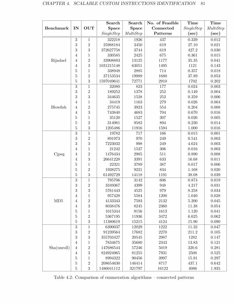
CHAPTER 4. SCALABLE CUSTOM INSTRUCTIONS IDENTIFICATION 81
Search Search No. of Feasible Time TimeBenchmark IN OUT Space Space Connected SingleStep MultiStep
SingleStep MultiStep Patterns (sec) (sec)
Rijndael
3 1 322218 1926 437 0.339 0.0123 2 25988184 3450 619 27.10 0.0213 3 372627758 3744 619 427.2 0.0304 1 330585 2425 675 0.361 0.0154 2 33908883 13125 1177 35.35 0.0414 3 1031215148 63051 1495 1121 0.1435 1 338948 2885 714 0.357 0.0185 2 37153534 19989 1680 37.89 0.0535 3 1597049641 72771 2910 1702 0.202
Blowfish
3 1 32080 823 177 0.024 0.0033 2 189252 1378 252 0.149 0.0043 3 344635 1528 252 0.359 0.0064 1 34419 1163 279 0.026 0.0044 2 275745 3923 554 0.204 0.0084 3 743840 4683 704 0.670 0.0165 1 35120 1527 307 0.026 0.0055 2 314981 9582 894 0.230 0.0145 3 1205486 11916 1594 1.000 0.016
Cjpeg
3 1 19782 717 166 0.015 0.0013 2 891973 970 249 0.541 0.0033 3 7223032 998 249 4.624 0.0034 1 21242 1537 306 0.016 0.0034 2 1476434 2985 511 0.890 0.0084 3 26641228 3391 633 16.68 0.0115 1 22321 3789 387 0.017 0.0065 2 1938275 9221 834 1.168 0.0205 3 61492729 14118 1191 38.08 0.039
MD5
3 1 795706 3142 606 0.874 0.0193 2 3349367 4399 948 4.217 0.0313 3 5761443 4525 979 8.258 0.0344 1 957428 5584 1200 1.040 0.0284 2 4133343 7593 2132 5.200 0.0454 3 8038476 8245 2360 11.38 0.0545 1 1015344 9156 1613 1.120 0.0415 2 5367195 11936 3472 6.625 0.0625 3 11380619 15215 4124 15.90 0.090
Sha(unroll)
3 1 6390037 12029 1222 11.32 0.0473 2 91239564 17682 2270 211.2 0.1053 3 355703427 20545 2987 1282 0.1474 1 7834675 35680 2343 13.83 0.1214 2 147686544 57246 5019 320.6 0.2814 3 824924965 81255 7931 2508 0.5255 1 8994322 90456 3997 15.91 0.2975 2 208654630 146414 8717 437.1 0.6425 3 1486041112 321797 16122 4086 1.935
Table 4.2: Comparison of enumeration algorithms – connected patterns

CHAPTER 4. SCALABLE CUSTOM INSTRUCTIONS IDENTIFICATION 82
1424087217839 8426
0000
3/1
28 46
241
1290
37
180136
2011
60
1541
243
2437
114
862
26
111 116
1141
42
1516
211
4777
27
54
715
58107
681
63
976
177
2112
100
1000
10
Spee
dup
3/1
3/2
3/3
4/1
4/2
4/3
8 15
24
75
2620
53
2716
1 10
Rijndael Blowfish Cjpeg MD5 Sha(unroll)
S
5/1
5/2
5/3
139 243
1761
61
113
657 471
128 117 154
1170
114 115 113
77
471
84 89
411
98 79
62 63
331 279
0010
00up
3/1
3/2
3/3
4/137
21 20
61 41
50 42
7
43
22 16
6
26
14
37 54 62
16
63 52 60
9 6 10
1Sp
eedu 4/1
4/2
4/3
5/1
5/2
5/3
1
Rijndael Blowfish Cjpeg MD5 Sha(unroll)
Figure 4.7: Run time speedup (MultiStep/SingleStep) for connected patterns.
to the size of the regions, the number of feasible connected patterns is quite small.
Therefore, it is possible to apply an optimal selection method, such as the ILP
formulation in Chapter 5, in the later stage for an optimal set of custom instructions.
The “Search Space” columns are the number of patterns subjected to different
constraint checks by the two algorithms. In general, as MultiStep algorithm pro-
duces connected patterns by extending existing ones with neighbors, it is far more
effective in pruning infeasible patterns. The last two columns presents the actual
execution time of the two algorithms. MultiStep algorithm takes at most seconds to
get connected feasible patterns in all cases, while SingleStep algorithm sometimes
require thousands of seconds (e.g., 5-input 3-output cases of Rijndael and Sha).
Run time speedups of MultiStep algorithm over SingleStep is shown in Figure 4.7.
4.3.3 Comparison on All Feasible Pattern Enumeration
The third step of MultiStep algorithm generates all feasible disjoint MIMO pat-
terns. Meanwhile, for the SingleStep algorithm, the overhead of ensuring pattern

CHAPTER 4. SCALABLE CUSTOM INSTRUCTIONS IDENTIFICATION 83
Search Additional No. of Time TimeBenchmark IN OUT Space Combination Feasible SingleStep MultiStep
SingleStep MultiStep Patterns (sec) (sec)
Rijndael
3 1 412567 0 437 0.446 0.0123 2 33014612 116666 3612 36.99 0.0213 3 434738397 812455 3612 518.7 1.1024 1 424929 0 675 0.754 0.0154 2 44573604 169762 54203 54.85 0.4864 3 1280116614 13599267 66785 1564 18.545 1 437287 0 714 0.475 0.0185 2 49440953 176534 115434 56.75 0.7225 3 2095522364 26956483 520993 2296 43.93
Blowfish
3 1 65226 0 177 0.063 0.0033 2 430665 3354 522 0.547 0.0093 3 751917 11634 522 2.297 0.0184 1 70145 0 279 0.168 0.0044 2 645364 4580 2577 0.769 0.0184 3 1671412 44452 2937 5.534 0.0625 1 71550 0 307 0.069 0.0055 2 746739 4608 4728 1.662 0.0275 3 2876509 73442 8428 7.498 0.126
Sha(unroll)
3 1 6391404 0 1222 11.41 0.0473 2 94121024 79072 6172 217.6 0.3313 3 365542922 515750 9796 1328 1.1354 1 7836042 0 2343 13.93 0.1214 2 152320527 116723 38728 331.5 0.7044 3 866118119 3905462 78566 2616 6.3595 1 8995689 0 3997 15.91 0.2975 2 215044666 166911 82022 449.8 1.3605 3 7577280675 7487850 280809 4312 15.44
Cjpeg
3 1 34715 0 166 0.020 0.0013 2 2571515 39945 911 1.507 0.0373 3 37250374 228304 960 22.53 0.1924 1 37343 0 306 0.022 0.0034 2 4234944 84718 13590 2.485 0.1134 3 122703827 4771054 18180 73.35 4.6625 1 39406 0 387 0.223 0.0065 2 5571468 116771 37603 3.277 0.2105 3 271219380 15162301 142348 161.4 17.68
MD5
3 1 996513 0 606 2.632 0.0193 2 4489507 75841 1255 17.58 0.1553 3 8210790 118955 1328 37.92 0.2474 1 1124690 0 1200 3.186 0.0284 2 7006628 110519 43106 27.36 0.3544 3 13460076 6703984 46028 60.60 9.7455 1 1194981 0 1613 4.030 0.0415 2 9730310 134698 79737 34.27 0.5435 3 21367000 9921718 119155 90.94 15.38
Table 4.3: Comparison of enumeration algorithms – disjoint patterns

CHAPTER 4. SCALABLE CUSTOM INSTRUCTIONS IDENTIFICATION 84
1424087217839 8426
0000
3/1
28 46
241
1290
37
180136
2011
60
1541
243
2437
114
862
26
111 116
1141
42
1516
211
4777
27
54
715
58107
681
63
976
177
2112
100
1000
10
Spee
dup
3/1
3/2
3/3
4/1
4/2
4/3
8 15
24
75
2620
53
2716
1 10
Rijndael Blowfish Cjpeg MD5 Sha(unroll)
S
5/1
5/2
5/3
139 243
1761
61
113
657 471
128 117 154
1170
114 115 113
77
471
84 89
411
98 79
62 63
331 279
0010
00up
3/1
3/2
3/3
4/137
21 20
61 41
50 42
7
43
22 16
6
26
14
37 54 62
16
63 52 60
9 6 10
1Sp
eedu 4/1
4/2
4/3
5/1
5/2
5/3
1
Rijndael Blowfish Cjpeg MD5 Sha(unroll)
Figure 4.8: Run time speedup (MultiStep/SingleStep) for all feasible patterns.
connectivity in previous experiments is removed. However, its search space is also
increased because it works on the entire DFG instead of individual regions.
The results are shown with Table 4.3. The “Additional Combination Multi-
Step” is the total number of pattern pairs subject to various checks in the third
step of MultiStep algorithm. When output constraint is 1, no additional combina-
tion is required because the third step is not performed. Each valid node has at
least 1 output, hence a 1-output pattern must also be a connected one. The time
to produce all feasible patterns is compared in the last 2 columns. Due to reasons
discussed in Section 4.2.2, MultiStep is faster than SingleStep by orders of 10X to
1000X. Detailed speedup numbers are shown in Figure 4.8. The “No. of Feasible
Patterns” column is obtained by summing up the total number of connected pat-
terns and disjoint patterns. As can be seen, the number of all the feasible patterns
is far greater than that of connected ones in most cases. For example, the number
of patterns increases 179 times for Rijndael and 120 times for Sha in 5-input, 3-
output cases, respectively. The large number of feasible patterns renders optimal
custom instruction selection methods seemingly infeasible. Heuristics to filter out

CHAPTER 4. SCALABLE CUSTOM INSTRUCTIONS IDENTIFICATION 85
most insignificant subgraphs are then crucial to cut down the search space. For
example, Sun [77] removes patterns with priority values that do not meet a certain
percentage of the best discovered candidate so far. Note however, pruning unvalued
patterns after exhaustive enumeration is not the same as using heuristics for enu-
meration right from the beginning. Exhaustive enumeration provides a complete
set of patterns for reuse and scheduling possibilities, which cannot be provided by
current enumeration heuristics.
4.4 Summary
In this chapter, we have described a scalable algorithm that exhaustively enumer-
ates all feasible candidate patterns for custom instructions under architectural con-
straints. These patterns will be organized in a pattern library according to topology
isomorphism. Because all the feasible patterns are enumerated, all the isomorphic
patterns embedded inside the DFG can be exposed to the pattern selection process,
which is then able to explore better custom instruction reuse. The result is that
fewer custom instructions would be necessary to cover the application for optimized
performance.
Furthermore, the greatly reduced running time of the enumeration process pro-
vides opportunity to explore large DFGs, either from datapath intensive applications
or ones resulting from modern compiler transformations. It makes it possible to in-
tegrate optimal custom instruction selection into state-of-the-art ISEP tool chains
in the early stage of the design.
Finally, input/output and convexity constraints are the most general and mini-
mal constraints on the dataflow subgraphs for CFU implementation. The specialty

CHAPTER 4. SCALABLE CUSTOM INSTRUCTIONS IDENTIFICATION 86
of particular CFU architectures, if any, can further cut down the number of can-
didates for the later custom instruction selection phase. It can be applied in the
enumeration process to further cut down the search space, or directly on the com-
plete set of enumerated subgraphs to obtain the conforming ones.
Chapter 5
Custom Instruction Selection
Look beyond what you see. – Rafiki, in “Lion King 1/2”
The second subproblem of custom instruction identification is custom instruc-
tion selection. Only a subset of the enumerated candidate patterns (subgraphs)
will be selected for custom instructions due to resource constraints on custom in-
structions and custom functional units. Other constraints, such as schedulability
of the custom instruction, or that a base operation should be covered by at most
one custom instruction, also need to be satisfied in order to guarantee proper code
generation. In this chapter, we first define and formulate the custom instruction
selection problem using integer linear programming (ILP) formulation for the max-
imum performance. Based on our custom instruction identification methodology,
we carry out a systematic study to evaluate how different values of various typical
design constraints will impact the system performance. This study is set out to
provide a valuable reference for the design of general extensible processors.
87

CHAPTER 5. CUSTOM INSTRUCTION SELECTION 88
5.1 Custom Instruction Selection
Given the set of candidate subgraphs, we first identify the isomorphic subgraphs
and build the pattern library. A template pattern represents the group of isomor-
phic subgraphs that can be mapped to the same custom instruction or CFU; each
occurrence of the subgraph is an instance of the pattern. The execution frequen-
cies of subgraph instances are different and results in different performance gains.
The selection process attempts to cover each original instruction in the code with
zero/one custom instruction to maximize performance.
5.1.1 Optimal Custom Instruction Selection using ILP
Let us first define the variables. We have N custom instructions defined by C1 . . . Cn.
A custom instruction Ci can have ni different instances occurring in the program
denoted by ci.1 . . . ci.ni. Each instance has execution frequency given by fi.j. Let Ri
be the area requirement of the custom instruction Ci and Pi be the performance
gain obtained by implementing Ci in hardware as opposed to software (given in
number of clock cycles). Finally, we define binary variables si.j which is equal to 1 if
custom instruction instance ci.j is selected and 0 otherwise. The objective function
maximizes the total performance gain using custom instructions:
max :N∑
i=1
ni∑j=1
(Pi × fi.j × si.j)
We optimize the objective function under the constraint that a primitive opera-
tion can be covered by at most one custom instruction instance. If custom instruc-
tion instances ci1.j1 . . . cik.jkcan cover a particular primitive operation, then
si1.j1 + . . .+ sik.jk≤ 1

CHAPTER 5. CUSTOM INSTRUCTION SELECTION 89
AND XOR
OR
XOR_ADD
ADD
AND
OR
XOR
AND
OR
(a) (b) (c)
Figure 5.1: Subgraph convexity. (a) A non-convex subgraph, (b) Two interdepen-dent convex subgraphs, (c) The left subgraph turns non-convex after the right one isreduced to a custom instruction; consequently the left subgraph cannot be selected.
In order to model the area constraint or the constraint on the total number of
custom instructions, we first define the variable Si. Si is the binary variable which
is equal to 1 if Ci is selected and 0 otherwise. Si is defined in terms of si.j.
Si = 1 if
ni∑j=1
si.j > 0
= 0 otherwise
However, the above equation is not a linear one. We substitute it with the
following equivalent linear equations.
ni∑j=1
si.j − U × Si ≤ 0
ni∑j=1
si.j + 1− Si > 0
where U is a large constant greater than ni.
It is not sufficient to ensure the convexity of each individual subgraph. As shown
with Figure 5.1 (b) and (c), two non-overlapping convex subgraphs interdependent

CHAPTER 5. CUSTOM INSTRUCTION SELECTION 90
on each other cannot be both selected. For each pair of interdependent subgraphs
ci.j and ci′.j′ , then we have
si.j + si′.j′ ≤ 1
Or let ck.l, . . . , cm.n be the set of subgraphs non-overlapping and interdependent
with ci.j, we have
sk.l + . . .+ sm.n = 0 if si.j = 1
= don′t− care otherwise
We linearize it as
sk.l + . . .+ sm.n ≤ U × (1− si.j)
If R is the total area budget for all the CFUs, then
N∑i=1
(Si ×Ri) ≤ R
Similarly, if M is the constraint on the total number of custom instructions, then
N∑i=1
Si ≤M
5.1.2 Experiments on the Effects of Custom Instructions
We use the same set of benchmarks used in Chapter 4 as shown in Table 5.1. They
are compiled under SimpleScalar tool set using SimpleScalar ported gcc-2.7.2.3 with
-O3 optimization. The last column shows the number of valid operations within
each of these basic blocks that can be potentially accelerated by custom instructions.
The remaining operations, being invalid ones, account for roughly 20% of the total
operations.

CHAPTER 5. CUSTOM INSTRUCTION SELECTION 91
BenchmarkBB Number ofSize valid nodes
rijndael 894 647blowfish 334 255
cjpeg 154 135MD5 943 723
sha(unroll) 1468 1368
Table 5.1: Benchmark characteristics.
We consider only the connected patterns here. For each benchmark, all feasible
connected subgraphs satisfying given number of input/output operands constraints
are enumerated. Then we form the pattern library based on the isomorphism check
algorithm described in [43]. At last, we build the ILP formulation. ILP formula-
tions are solved using ILOG CPLEX (v9.1), which is the leading commercial linear
programming solver, to obtain the optimal custom instructions for these big basic
blocks.
We calculate hardware latency and area for each of the base operations in the
SimpleScalar ISA using Synopsys design tool with a popular cell library. The hard-
ware latency of a custom instruction is approximated as the summation of the hard-
ware latencies of the operations along the critical path of its dataflow graph, and the
area simply as the summation of the hardware area of the constituent operations.
Note that the approximations are actually pessimistic because combined logic can
be optimized for both latency and area. Execution cycles of a custom instruction
is computed by normalizing its latency (rounded up to an integer) against that of a
multiply-accumulate (MAC) operation, which we assume takes exactly one cycle.
To evaluate the effects of custom instructions on system performance, we cal-
culate the percentage of cycle reduction. We use a single-issue, in-order pipelined
architecture with 100% cache hit rate. As many of the recent embedded proces-
sors, such as ARM11 and PowerPc602, are in-order processors, this is an realistic
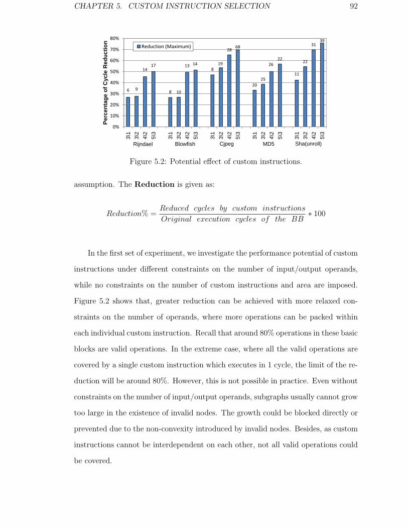
CHAPTER 5. CUSTOM INSTRUCTION SELECTION 92
2868 31
39
70%
80%
ctio
n
Reduction (Maximum)
6 9
1417
8 10
13 148
19
2025
2622
11
22
20%
30%
40%
50%
60%
age
of C
ycle
Red
u
0%
10%
20%
3\1
3\2
4\2
5\3
3\1
3\2
4\2
5\3
3\1
3\2
4\2
5\3
3\1
3\2
4\2
5\3
3\1
3\2
4\2
5\3
Perc
enta
Rijndael Blowfish Sha(unroll)Cjpeg MD5
1417 13 14
8
19
2868
2622
11
22
3139
55 5
76
7
910
2019
8
9
77
50%
60%
70%
80%
cle
Red
uctio
n Reduction (Maximum)Reduction (Effective)
6 9 8 1020
25
3 5 4 3
1315
8
0%
10%
20%
30%
40%
Perc
enta
ge o
f Cyc
0%
3\1
3\2
4\2
5\3
3\1
3\2
4\2
5\3
3\1
3\2
4\2
5\3
3\1
3\2
4\2
5\3
3\1
3\2
4\2
5\3
Rijndael Blowfish Sha(unroll)Cjpeg MD5
Figure 5.2: Potential effect of custom instructions.
assumption. The Reduction is given as:
Reduction% =Reduced cycles by custom instructions
Original execution cycles of the BB∗ 100
In the first set of experiment, we investigate the performance potential of custom
instructions under different constraints on the number of input/output operands,
while no constraints on the number of custom instructions and area are imposed.
Figure 5.2 shows that, greater reduction can be achieved with more relaxed con-
straints on the number of operands, where more operations can be packed within
each individual custom instruction. Recall that around 80% operations in these basic
blocks are valid operations. In the extreme case, where all the valid operations are
covered by a single custom instruction which executes in 1 cycle, the limit of the re-
duction will be around 80%. However, this is not possible in practice. Even without
constraints on the number of input/output operands, subgraphs usually cannot grow
too large in the existence of invalid nodes. The growth could be blocked directly or
prevented due to the non-convexity introduced by invalid nodes. Besides, as custom
instructions cannot be interdependent on each other, not all valid operations could
be covered.

CHAPTER 5. CUSTOM INSTRUCTION SELECTION 93
2868 31
39
70%
80%
ctio
n
Reduction (Maximum)
6 9
1417
8 10
13 148
19
2025
2622
11
22
20%
30%
40%
50%
60%
age
of C
ycle
Red
u
0%
10%
20%
3\1
3\2
4\2
5\3
3\1
3\2
4\2
5\3
3\1
3\2
4\2
5\3
3\1
3\2
4\2
5\3
3\1
3\2
4\2
5\3
Perc
enta
Rijndael Blowfish Sha(unroll)Cjpeg MD5
1417 13 14
8
19
2868
2622
11
22
3139
55 5
76
7
910
2019
8
9
77
50%
60%
70%
80%
cle
Red
uctio
n Reduction (Maximum)Reduction (Effective)
6 9 8 1020
25
3 5 4 3
1315
8
0%
10%
20%
30%
40%
Perc
enta
ge o
f Cyc
0%3\
13\
24\
25\
3
3\1
3\2
4\2
5\3
3\1
3\2
4\2
5\3
3\1
3\2
4\2
5\3
3\1
3\2
4\2
5\3
Rijndael Blowfish Sha(unroll)Cjpeg MD5
Figure 5.3: Effect of custom instructions.
The numbers on top of each bar in Figure 5.2 show the numbers of custom
instructions (pattern templates) required to achieve the maximum cycle reductions.
As ILP formulation is single objective, while maximizing cycle reduction, it does not
minimize the values of its constraints. Without constraining the number of custom
instructions (or area), the ILP solver simply produces one feasible assignment of
variables that first reaches the optimal objective. Isomorphisms among the sub-
graphs are not fully exploited. Consequently, the numbers of custom instructions
required are quite large (e.g., 68 custom instructions for Cjpeg).
In practice, we do not need to exhaust every single cycle reduction at an un-
necessary cost level. Instead, we are often more interested in exploiting most of
the cycle reduction with minimum number of custom instructions, which we call
effective cycle reduction. To achieve this, we solve the ILP formulations multiple
times by trying different values on the number of custom instructions constraint,
until we find the minimum number that can obtain more than a certain percentage
of the maximum reduction (95% in our case). After that, we increase the number of
custom instructions one at a time, until the additional reduction obtained becomes
less than a certain variance (1% of the maximum reduction in our case). Figure 5.3
shows the results of effective reduction. In general, much less number of custom
CHAPTER 5. CUSTOM INSTRUCTION SELECTION 94
instructions are required to achieve more than 95% of the maximum reduction. For
example, 10 custom instructions instead of 68 yield more than 99% of the maximum
reduction for Cjpeg under 5-input 3-output operands constraint. In some cases, ef-
fective reductions are the same as the maximum reductions. The tightened number
of custom instructions constraint simply enforces the use of isomorphic subgraphs.
5.2 A Study on the Potential of Custom Instruc-
tions
Based on our custom instruction identification methodology, in this section, we in-
vestigate the potential of performance improvement using custom instructions under
relaxed design constraints. We vary the design constraints from very restricted to
very relaxed. This allows us to systematically study the effects of different de-
sign constraints and provides insights on the relative importance of these design
restrictions. These constraints, which come from architectural, cost, and compiler
limitations and affect the choice of custom instructions, are listed as follows:
• Number of Operands: The performance speedup of a custom instruction
typically increases with increasing number of operands. However, it may be
difficult to accommodate large number of operands in the standard format of
the base ISA. Moreover, the number of input and output ports to the register
file has to be proportional to the number of input and output operands required
by an instruction. The cost and energy consumption of a processor increase
significantly with increasing number of register file ports. These considerations
may impose limits on the maximum number of operands.
• Number of custom instructions: The instruction format of the base ISA
may limit the number of custom instructions that can be introduced. For
CHAPTER 5. CUSTOM INSTRUCTION SELECTION 95
example, if the base ISA implements 26 instructions using fixed length 5-bit
opcode, then it can accommodate six new instructions.
• Area: As cost is a major consideration for embedded systems, only a limited
amount to die area is expected to be available for the implementation of the
CFUs.
• Control Flow: Custom instruction identification is typically performed within
basic block boundaries. The assumption is that the compiler cannot exploit
instructions that cross basic block boundaries.
Among these constraints, we are particularly interested in the impact of relaxing
the control flow constraint. By identifying custom instructions across basic blocks,
their true performance potential under modern compiler techniques can be revealed.
Note that we do not consider run-time reconfiguration of CFUs in the study, as the
effect is similar to having no constraints on number of custom instructions and area.
Run-time reconfiguration can only be beneficial when performance improvement of
static configuration is well restricted by the above two constraints.
5.2.1 Crossing the Basic Block Boundaries
Most of the research in candidate pattern identification are based on analyzing the
basic blocks in isolation. The only exception to this is the work by Arnold and
Corporaal [6], which identifies patterns based on the dynamic execution trace of
the program. Dynamic execution trace is the record of the program’s complete run
time execution sequence. As we are interested in identifying the performance poten-
tial of customization, our identification process is also based on dynamic execution
trace. This way we can identify patterns and their frequencies across basic block
boundaries. Using execution trace we can group operations across branches in the

CHAPTER 5. CUSTOM INSTRUCTION SELECTION 96
(a) (b)
50 5050 50
BB0(100)
BB6(100)
BB3(100)
BB1(50) BB2(50)
BB4(50) BB5(50)
BB0(100)
BB6(100)
BB3(100)
BB1(50) BB2(50)
BB4(50) BB5(50)
Figure 5.4: Possible correlations of branches. (a) Left (right) side of the 1st branchis always followed by the left (right) side of the 2nd one, (b) Left (right) side of the1st branch is always followed by the right (left) side of the 2nd one.
execution sequence more accurately. This is because certain dynamic behavior can-
not be deduced from profiling of basic block execution counts. Figure 5.4 shows an
example control flow graph where correlation of biased branches cannot be correctly
inferred from only the execution counts. However, Arnold [6] constructs a huge
dataflow graph for the entire trace and builds patterns incrementally by traversing
this graph multiple times. This approach is computationally expensive, thereby lim-
ited to small patterns. Instead we base our study on a compact representation of
the dynamic execution trace called Whole Program Path (WPP) [48], which allows
identification of patterns within and across basic blocks in an efficient manner.
Whole Program Path (WPP)
Larus developed the notion of Whole Program Path (WPP) [48], which captures
the entire execution trace of a program. The storage overhead for the trace is
reduced drastically by employing on-line string compression techniques called SE-
QUITUR [60]. SEQUITUR algorithm represents a finite string σ (the control flow

CHAPTER 5. CUSTOM INSTRUCTION SELECTION 97
S(1)
S AACC7A BBB 01346
Interior node(basic block
)
S(1)
B 01346C 02356
sequence)A(2)
B(4) C(2)
L f dLeaf node(basic block)
0(6) 1(4) 2(2) 3(6) 4(4) 5(2) 6(6) 7(1)
Figure 5.5: WPP for basic block sequence 0134601346013460134602356023567 withexecution count annotations.
trace in our case) as a context free grammar whose language is the singleton set {σ}.
The grammar is synthesized on-the-fly with time complexity linear in the length of
the input string. It works by appending symbols from the input string, in order, to
the end of the grammar’s start production. Upon each addition, SEQUITUR adjusts
the grammar to preserve the following two invariants. The first invariant is referred
to as the Diagram Uniqueness property, where a pair of consecutive symbols, called
a diagram, should occur at most once in the rules of the grammar. If adding a
symbol from the input string introduces a recurring diagram, its occurrences will
be replaced with the non-terminal symbol for a rule (possibly already constructed)
with the diagram as its right side. This first invariant constructs the rules and builds
the hierarchy to express the redundancy. The second invariant is referred to as the
Rule Utility property, where all non-terminal symbols of the grammar (except for
the start symbol) must be referred more than once by other rules; otherwise, a rule
will be eliminated. The reference count of a non-terminal symbol may reduce when
its occurrence is replaced by other non-terminal symbols on the higher hierarchy.
The second invariant eliminates the useless rules.
The execution trace of a program can be viewed as a string over an alphabet
CHAPTER 5. CUSTOM INSTRUCTION SELECTION 98
of basic blocks. The grammar produced by SEQUITUR can be represented as a
directed acyclic graph (DAG), called WPP. Figure 5.5 shows an example of WPP.
Each node of the WPP is annotated by the execution count of the sub-DAG rooted
at that node. The leaf nodes of the WPP are the basic blocks; an interior node
represents a sequence of basic blocks appearing in the execution trace. This example
illustrates how the correlations of the two branches in Figure 5.4(a) can be captured
in the WPP (by non-terminal symbols B and C).
During candidate pattern enumeration, we first start with the basic blocks and
identify subgraphs within the basic blocks. To identify subgraphs across basic block
boundaries, we look at frequently occurring interior nodes in the WPP and treat
the sequence of basic block corresponding to that node as the unit for pattern
identification process.
5.2.2 Experimental Setup
Table 5.2 shows the benchmark programs used in this study. All the benchmarks,
except for md5, are from MiBench [31]: a free, representative embedded benchmark
suite. We have selected benchmark programs from all the different categories such as
security, network, telecomm etc. We consider integer-intensive benchmarks here, as
including float-point operations in patterns seldom results in speedup. Table 5.2 also
shows the total number of basic blocks and hot basic blocks for each program. We
define hot basic blocks as the ones whose aggregate contribution exceed 95% of the
total execution time of the program. ISE identification methodology only explores
these hot basic blocks and basic block sequences involving them. Including patterns
from the rest of the basic blocks has negligible effect on performance improvement.
The average size of hot basic blocks varies from very small (2.6 instructions) to very
big (495.7 instructions).

CHAPTER 5. CUSTOM INSTRUCTION SELECTION 99
Benchmark Class Total Hot Avg. HotBB BB BB Size
rawcaudio Telecomm 68 22 2.6rawdaudio Telecomm 66 18 2.6fft Telecomm 129 24 6.8sha Security 76 6 17.2strsearch Office 148 4 6qsort Automotive 30 26 4.9bitcnts Automotive 79 13 12.4basicmath Automotive 94 28 6patricia Network 203 37 2.8dijkstra Network 77 6 5djpeg Consumer 317 96 6.8rijndael Security 168 7 184.3blowfish Security 81 13 30.3sha(unroll) Security 68 3 495.7cjpeg Consumer 3756 145 7.8md5 Security 107 39 29.6
Table 5.2: Characteristics of benchmark programs
The execution traces of the programs are generated using Simplescalar tool
set [12] which is a cycle-accurate simulation platform for RISC-like processor archi-
tectures. The benchmarks are compiled by gcc version 2.7.2.3 with -O3 optimization.
We build the Whole Program Path (WPP) from the execution traces using a modi-
fied version of the Sequitur grammar [59]. DFGs for the hot basic blocks and paths
(internal nodes of WPP) are constructed to identify custom instructions within and
spanning across multiple basic blocks. Only connected candidate subgraphs are
enumerated. The ILP formulations for custom instruction selection are solved us-
ing ILOG CPLEX (v9.1). There are cases (a few ones for sha(unroll) and md5)
for which CPLEX cannot return their optimal cycle reductions within 2 hours on a
3Ghz Pentium4 Linux workstation. For these cases, we use the best cycle reductions
CPLEX have achieved with 2 hours running time, which are provable to be at most
5% less than the optimal ones.
Evaluation of latencies and area of custom instructions is the same as that
described in Section 5.1.2. Similarly, under the assumption of a single-issue, in-order

CHAPTER 5. CUSTOM INSTRUCTION SELECTION 100
pipelined architecture with 100% cache hit rate, the percentage of cycle reduction
is given as:
Reduction% =Reduced cycles by custom instructions
Original execution cycles of the benchmark∗ 100
5.2.3 Results and Analysis
We describe the findings of the limit study in this section. We first look at the reduc-
tion obtained by limiting the patterns to basic blocks. Later, we explore reduction
achievable with patterns that can cross basic block boundaries.
Operand Constraint
The restriction on number of operands either comes from inherent limitations of the
ISA or the register file design decisions of the base processor. However, sometimes
this is an artificial restriction imposed by the tool that automatically selects the
extensions in order to prune the deign space [67, 30]. The most popular choices are
(1) 2-input, 1-output patterns and (2) multiple-input single-output (MISO) patterns.
We investigate how these choices affect the cycle reduction due to extended ISA.
First, we restrict the patterns to 2-input, 1-output without imposing any other
constraint. The results indicate that for most benchmarks, it is extremely difficult
to find any such pattern. Even for benchmarks for which such patterns exist, the
reduction is insignificant (maximum is around 3.1% for dijkstra). However, we
observe that as memory operations are not allowed within a pattern, we cannot
exploit 2-input, 1-output structures like x = a[i].
Figure 5.6 shows the reduction with MISO and MIMO (multiple-input, multiple-
output) instructions. While we put very relaxed constraints on the number of inputs

CHAPTER 5. CUSTOM INSTRUCTION SELECTION 101
50%
60%MISOMIMO(2-out)
20%
30%
40%
50%
Red
uctio
n
MIMO(2 out)MIMO(3-out)
0%
10%
raw
caud
io
raw
daud
io fft
sha
strs
earc
h
qsor
t
bitc
nts
basi
cmat
h
patri
cia
dijk
stra
djpe
g
rijnd
ael
blow
fish
cjpe
g
MD
5
sha(
unro
ll)
40%
50%
60%
n
rawcaudiorawdaudiofftshastrsearchqsortbitcntsbasicmath
t i i
0%
10%
20%
30%
Red
uctio
patriciadijkstradjpegrijndaelblowfishcjpegmd5sha(unroll)
-10%2 3 4 5 6 inf
Number of Input
60%rawcaudiorawdaudio
20%
30%
40%
50%
Red
uctio
n
rawdaudiofftshastrsearchqsortbitcntsbasicmathpatriciadijkstradjpegrijndaelblowfishcjpeg
-10%
0%
10%
2 3 4 5 6 inf
R
Number of Input
jp gmd5sha(unroll)
Figure 5.6: Comparison of MISO and MIMO.
(10-inputs for the last 5 benchmarks, and infinite for the rest), we study the per-
formance impact of number of outputs by varying it from one to three. For all the
benchmarks, identifying custom instructions beyond three outputs results in little
or no further reduction. Thereby, the reduction for 3-output MIMO instructions can
almost represent the theoretical limit of the reduction obtainable when the patterns
are restricted to basic blocks. Except for strsearch, which has little reduction with
MISO instructions, in average, MIMO achieves 48.9% more cycle reduction than
that by MISO1. We also observe that the majority of the benchmarks achieve the
theoretical reduction with only 2 output operands.
As the number of output operands can be easily restricted to two, we vary the
number of input operands while the number of output operands is set to one or two
(see Figure 5.7) with no other restrictions. As we can see from the figure, 4-input
operands seem most effective to achieve reasonable reductions. We conclude that
even though 2-input, 1-output is quite a restrictive option, 4-input, 2-output can
achieve the marjority of the reductions.
1The number is relative to the reduction of MISO instructions. For example, for cjpeg from15.1% (MISO) to 23.1% (MIMO 3-out), MIMO achieves 53.1% more reduction than that of MISO.
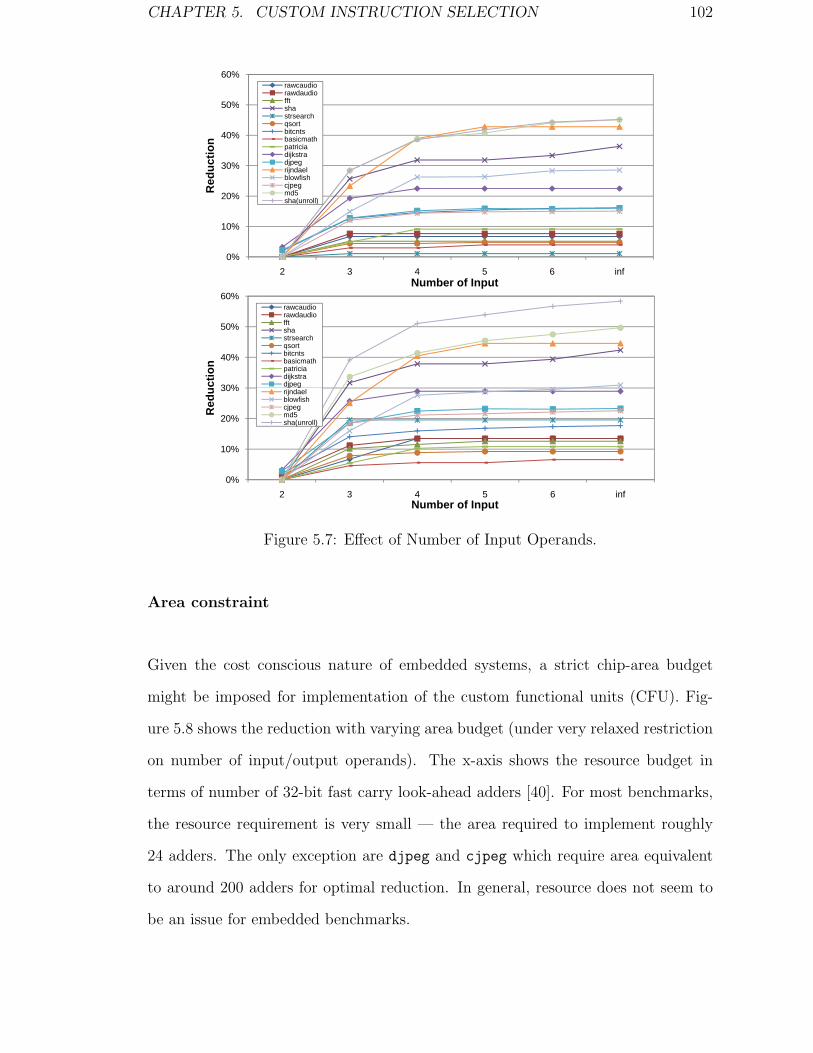
CHAPTER 5. CUSTOM INSTRUCTION SELECTION 102
50%
60%rawcaudiorawdaudiofft
20%
30%
40%
50%
Red
uctio
n
shastrsearchqsortbitcntsbasicmathpatriciadijkstradjpegrijndaelblowfishcjpegmd5sha(unroll)
0%
10%
2 3 4 5 6 infNumber of Input
sha(unroll)
30%
40%
50%
60%
ctio
n
rawcaudiorawdaudiofftshastrsearchqsortbitcntsbasicmathpatriciadijkstradjpeg
0%
10%
20%
30%
Red
u jp grijndaelblowfishcjpegmd5sha(unroll)
2 3 4 5 6 infNumber of Input
50%
60%rawcaudiorawdaudiofft
20%
30%
40%
50%
Red
uctio
n
shastrsearchqsortbitcntsbasicmathpatriciadijkstradjpegrijndaelblowfishcjpegmd5sha(unroll)
0%
10%
2 3 4 5 6 infNumber of Input
sha(unroll)
30%
40%
50%
60%
ctio
n
rawcaudiorawdaudiofftshastrsearchqsortbitcntsbasicmathpatriciadijkstradjpeg
0%
10%
20%
30%
Red
u jp grijndaelblowfishcjpegmd5sha(unroll)
2 3 4 5 6 infNumber of Input
Figure 5.7: Effect of Number of Input Operands.
Area constraint
Given the cost conscious nature of embedded systems, a strict chip-area budget
might be imposed for implementation of the custom functional units (CFU). Fig-
ure 5.8 shows the reduction with varying area budget (under very relaxed restriction
on number of input/output operands). The x-axis shows the resource budget in
terms of number of 32-bit fast carry look-ahead adders [40]. For most benchmarks,
the resource requirement is very small — the area required to implement roughly
24 adders. The only exception are djpeg and cjpeg which require area equivalent
to around 200 adders for optimal reduction. In general, resource does not seem to
be an issue for embedded benchmarks.

CHAPTER 5. CUSTOM INSTRUCTION SELECTION 103
50%
60%rawcaudiorawdaudio
20%
30%
40%
50%
Red
uctio
n
fftshastrsearchqsort-exambitcntsbasicmathpatriciadijkstradjpeg
200
0%
10%
20%
4 8 12 16 24 32 40 infResource (# of 32-bit adders)
jp grijndaelblowfishcjpegmd5sha(unroll)
Figure 5.8: Effect of area constraint.
50%
60%No. instr = infNo. instr = 5
20%
30%
40%
50%
Red
uctio
n
No. instr = 4No. instr = 3No. instr = 2No. instr = 1
0%
10%
raw
caud
io
raw
daud
io fft
strs
earc
h
qsor
t
basi
cmat
h
patri
cia
dijk
stra
sha
bitc
nts
djpe
g
rijnd
ael
blow
fish
cjpe
g
md5
sha(
unro
ll)
Figure 5.9: Effect of constraint on total number of custom instructions.
Total instructions constraint
Some extensible processors impose a limit on the total number of custom instruc-
tions that can be added. To illustrate this concern in the study, we vary the total
number of custom instruction constraint from 1 to 5 for each benchmark. As shown
in Figure 5.9, many benchmarks achieve maximum reduction under 5 instruction
constraint, while the others achieve the majority. Five instruction constraint may
not be good for some programs like djpeg and cjpeg whose datapaths vary a lot,
but effective enough for most others to exploit most of the benefits from custom

CHAPTER 5. CUSTOM INSTRUCTION SELECTION 104
instructions.
Control flow constraint
A common restriction imposed by most of the design automation tools is that the
patterns should be limited to basic blocks. The rationale being that it is hard
for the compiler to exploit patterns that span multiple basic blocks. We study
the performance potential that can be achieved by relaxing this constraint. Note
that as the kernel computation is already included in a few large basic blocks for
rijndael, blowfish, md5 and sha(unroll), there will be little difference exploiting
opportunities across basic blocks. Therefore, we omit these benchmarks in the
comparison here. Also, we must note that as we are using whole program path
to find hot paths consisting of multiple basic blocks, there is no artificial limit on
the number of basic blocks in a path. However, the experiments indicated that for
all the benchmarks opportunities exist only among 2–3 consecutive basic blocks.
The dataflow dependence is quite local and attempting to find patterns across more
basic blocks is not fruitful. However, patterns across 2–3 basic blocks can sometimes
achieve impressive improvement.
50%
60%MISO within BBMISO across BB
30%
40%
50%
Red
uctio
n
MIMO within BBMIMO across BB
0%
10%
20%
rawcaudio rawdaudio fft sha strsearch qsort bitcnts basicmath patricia dijkstra djpeg
40%
50%
60%
n
sha (within BB)
sha (across BB)
10%
20%
30%
Red
uctio
n
0%4 8 12 16 20 24 28 32 36 40 inf
Resource (# of 32-bit adder)
60%rawcaudiorawdaudio
30%
40%
50%
Red
uctio
n
rawdaudiofftshastringsearchqsortbitcntsbasicmathpatriciadijkstradjpeg
0%
10%
20%
2 3 4 5 6 inf
R
No of Input
Figure 5.10: Effect of relaxing control flow constraints.

CHAPTER 5. CUSTOM INSTRUCTION SELECTION 105
Figure 5.10 shows the effect of relaxing the control flow constraints for both
MISO and MIMO (no area constraint). In general, without the restriction of a
single output operand, MIMO patterns are more flexible, thus can exploit more
opportunities for performance improvement across basic block boundaries. Some
benchmarks (e.g., dijkstra) do not get any improvement by allowing patterns to
cross basic block boundaries. However, for others the relative improvement (relative
to the reduction of MISO and MIMO within basic blocks) ranges from a modest 5%
to as much as 95%.
50%
60%sha (within BB)sha (across BB)
20%
30%
40%
50%
Red
uctio
n
( )fft (within BB)fft (across BB)
0%
10%
20%
4 8 12 16 20 24 28 32 36 40 infResource (# of 32-bit adder)
40%
50%
60%
n
rawcaudiorawdaudiofftshastringsearchqsortbitcntsbasicmath
10%
20%
30%
Red
uctio
n patriciadijkstradjpeg
0%2 3 4 5 6 inf
No. of Input
Figure 5.11: Reduction across basic blocks under varying area budgets.
50%
60%sha (within BB)sha (across BB)
20%
30%
40%
50%
Red
uctio
n
( )fft (within BB)fft (across BB)
0%
10%
20%
4 8 12 16 20 24 28 32 36 40 infResource (# of 32-bit adder)
40%
50%
60%
n
rawcaudiorawdaudiofftshastringsearchqsortbitcntsbasicmath
10%
20%
30%
Red
uctio
n patriciadijkstradjpeg
0%2 3 4 5 6 inf
No. of Input
Figure 5.12: Effect of number of input operands under 3 outputs across basic blocks.
One question that may naturally arise is whether the resource consumption
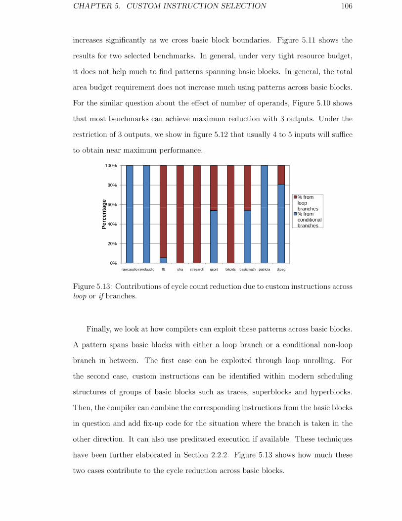
CHAPTER 5. CUSTOM INSTRUCTION SELECTION 106
increases significantly as we cross basic block boundaries. Figure 5.11 shows the
results for two selected benchmarks. In general, under very tight resource budget,
it does not help much to find patterns spanning basic blocks. In general, the total
area budget requirement does not increase much using patterns across basic blocks.
For the similar question about the effect of number of operands, Figure 5.10 shows
that most benchmarks can achieve maximum reduction with 3 outputs. Under the
restriction of 3 outputs, we show in figure 5.12 that usually 4 to 5 inputs will suffice
to obtain near maximum performance.
60%
80%
100%
age % from
loop b h
0%
20%
40%
rawcaudio rawdaudio fft sha strsearch qsort bitcnts basicmath patricia djpeg
Perc
enta branches
% from conditional branches
Figure 5.13: Contributions of cycle count reduction due to custom instructions acrossloop or if branches.
Finally, we look at how compilers can exploit these patterns across basic blocks.
A pattern spans basic blocks with either a loop branch or a conditional non-loop
branch in between. The first case can be exploited through loop unrolling. For
the second case, custom instructions can be identified within modern scheduling
structures of groups of basic blocks such as traces, superblocks and hyperblocks.
Then, the compiler can combine the corresponding instructions from the basic blocks
in question and add fix-up code for the situation where the branch is taken in the
other direction. It can also use predicated execution if available. These techniques
have been further elaborated in Section 2.2.2. Figure 5.13 shows how much these
two cases contribute to the cycle reduction across basic blocks.
CHAPTER 5. CUSTOM INSTRUCTION SELECTION 107
5.3 Summary
Custom instruction selection based on ILP formulation can make good use of isomor-
phic subgraphs which are exposed by exhaustive candidate enumeration. Due to this
benefit, a small set of custom instructions can be selected to cover the application
effectively to achieve near to theoretical performance improvement.
We have also studied the performance potential of extensible processors for a
broad range of embedded applications. Using a compressed execution trace based
methodology, we are able to investigate improvement for the ISE even under ex-
tremely relaxed conditions. The summary of our major findings are:
1. Relaxing control flow constraints can achieve 5–95% relative improvement for
the selected set of benchmarks without major impact on total resource re-
quirement. Most of this improvement can be realized with existing compiler
techniques such as predication and loop unrolling.
2. One can put a reasonable limit on resource and number of custom instructions
without affecting speedup.
3. Restrictions on number of operands (such as allowing only MISO or 2-input,
1-output patterns) can significantly limit the performance. However, 5-input,
3-output patterns achieve close to maximal cycle reduction.

Chapter 6
Improving WCET with Custom
Instructions
The man who invented the first wheel was an idiot. The man who
invented the other three, he was a genius. – Sid Caesar
A large portion of embedded systems are real-time systems. In a real-time
system, a task must meet its deadline for the system to operate properly or handle
critical missions responsively. In order to satisfy real-time constraints (deadlines),
the worst-case execution time (WCET) of a task should be reduced as opposed
to its average-case execution time. However, normal custom instruction selection
techniques based on profiling information aim to improve the average-case execution
time; these techniques may not reduce a task’s WCET. In this chapter, we explore
a novel application of instruction-set extensions to meet tight timing constraints in
real-time embedded systems.
108
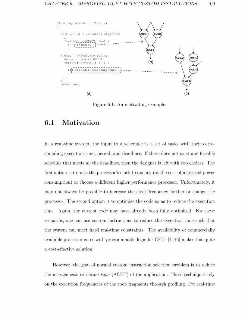
CHAPTER 6. IMPROVING WCET WITH CUSTOM INSTRUCTIONS 109
float expint(int n, float x){
…if(x > 1.0) { //Lentz’s algorithm
…for(i=1; i<=MAXIT; i++) {
a = -i*(nm1+i);…
}} else { //Evaluate series
ans = … -log(x)-EULER;for(i=1; i<=MAXIT; i++) {
…if( fabs(del)<fabs(ans)*EPS )…
}}return ans;
}
SUBUADDU
MULT
(a)
(b)
(c)
ABS.D
CMP.D
ABS.D
MUL.D
Figure 6.1: An motivating example.
6.1 Motivation
In a real-time system, the input to a scheduler is a set of tasks with their corre-
sponding execution time, period, and deadlines. If there does not exist any feasible
schedule that meets all the deadlines, then the designer is left with two choices. The
first option is to raise the processor’s clock frequency (at the cost of increased power
consumption) or choose a different higher performance processor. Unfortunately, it
may not always be possible to increase the clock frequency further or change the
processor. The second option is to optimize the code so as to reduce the execution
time. Again, the current code may have already been fully optimized. For these
scenarios, one can use custom instructions to reduce the execution time such that
the system can meet hard real-time constraints. The availability of commercially
available processor cores with programmable logic for CFUs [4, 75] makes this quite
a cost-effective solution.
However, the goal of normal custom instruction selection problem is to reduce
the average case execution time (ACET) of the application. These techniques rely
on the execution frequencies of the code fragments through profiling. For real-time

CHAPTER 6. IMPROVING WCET WITH CUSTOM INSTRUCTIONS 110
tasks, on the other hand, custom instructions should reduce the worst case execution
time (WCET). The WCET of a task is defined as its maximum execution time for all
possible inputs. Let us illustrate the difference with an example. Figure 6.1 shows
a code fragment that computes the value of the exponential integral. There are two
candidate patterns — one from each side of a conditional branch. Let us assume
that we can implement only one custom instruction. For reducing the ACET, the
pattern selection will depend on the frequency of execution of these two patterns.
However, this selection may not be beneficial for WCET reduction as the frequently
executed pattern may not contribute to the worst-case execution path. For example,
if the else part of the conditional branch contributes towards the worst case path,
then the pattern on the else part should be selected for WCET reduction.
Moreover, it is not sufficient to use the execution frequencies corresponding to
the WCET path and then employ the traditional custom instruction selection tech-
niques. The WCET path may not remain the same throughout the selection process.
Once we have selected some custom instructions to reduce the current WCET path,
a new path may become the WCET path. Therefore, custom instruction selection
problem for WCET reduction is more challenging compared to ACET reduction.
6.1.1 Related Work to Improve WCET
Compiler techniques to reduce the WCET of a program have started to receive
attention only very recently. Reduction of WCET in [53] is achieved through dual
instruction set ARM processor. Based on WCET path analysis, they consider apply-
ing the full length (32-bit) ARM instruction on the WCET path for faster execution,
whilst the reduced Thumb instruction set on the remaining code to save space and
energy. In [84], the influence of WCET upon different orders of compiler optimiza-
tion techniques is studied through a genetic algorithm approach. [85] presents a code
CHAPTER 6. IMPROVING WCET WITH CUSTOM INSTRUCTIONS 111
positioning method by trying to place basic blocks on WCET paths in continuous
position so as to avoid branch taken penalties on embedded processors. [83] reduces
WCET by applying superblock formation guided by WCET paths. Suhendra et al.
[76] minimizes the WCET by using scratch pad memory, which provides fast access
to data objects that are statically allocated to it hence with fully predictable timing.
Most of these works improve the current WCET path iteratively. They may miss
the global optima as closely competing paths are not considered simultaneously.
Here, we explore the possibility of using instruction-set extensions to improve
the WCET of real-time applications. We propose an ILP formulation for the optimal
solution, followed by heuristics with a more global perspective that selects a pattern
to reduce the WCET across all the paths.
6.2 Problem Formulation
Given an application, all possible feasible computation patterns are identified us-
ing techniques proposed in Chapter 4. Let us assume that we have identified N
candidate pattern templates in a program defined by C1 . . . CN . A template Ci can
have ni different instances occurring in the program denoted by ci.1 . . . ci.ni. Let Pi
be the performance gain obtained by implementing Ci in hardware as opposed to
software. Ri is the amount of area required to implement the CFU corresponding
to Ci. Suppose we have a constraint on the total number of custom instructions
that can be implemented in the architecture, say M (M < N). Then our goal is
to cover each original instruction in the code with zero/one instances of at most M
custom instructions, such that the WCET of the task is minimized. Similarly, we
may have a constraint that the total amount of area required by the selected custom
instructions should not exceed R.

CHAPTER 6. IMPROVING WCET WITH CUSTOM INSTRUCTIONS 112
A: seq
B: if
C: loop
9
1
2 3 F: loop
5 G: if
7
8
6
D: seq
4 E: func log
log(x)
if(x>1.0)1
for loop2
loop body3 for loop5
…7
…8
if(abs…)6
return ans9
T F
TF
4 …
(a) CFG (b) Syntax tree
Figure 6.2: CFG and syntax tree corresponding to the code in Figure 6.1
As we need to improve the WCET, the problem formulation is intrinsically
related to the method used for WCET estimation. We use the Timing Schema
approach to estimate the WCET of a task in this work.
6.2.1 WCET Analysis using Timing Schema
Timing schema is an efficient technique to estimate the WCET of a structured pro-
gram [63]. The structure of the program is represented as a hierarchical syntax
tree with basic blocks as leaf nodes and control structures (i.e., sequences, branches,
and loops) as interior nodes. The entire program is represented at the root of the
syntax tree. Figure 6.2 shows the control flow graph1 and syntax tree corresponding
to the code in Figure 6.1. An interior node corresponding to a conditional branch
(e.g., nodes B and G in Figure 6.2(b)) has at most three children. The first child
is the basic block containing the branch condition. The second and the third chil-
dren represent the code fragments corresponding to taken and non-taken branches
respectively. Loop construct (e.g., nodes C and F) is essentially a sequence node
1We build CFG for optimized assembly code. The figure uses source code for illustration purposeonly.

CHAPTER 6. IMPROVING WCET WITH CUSTOM INSTRUCTIONS 113
except for the first child as the loop entry basic block. Function calls are represented
by leaf nodes (e.g., node E). A separate syntax tree is constructed for each function.
The entire program is represented as a syntax forest.
WCET of a program is estimated by traversing its hierarchical syntax tree in
a bottom-up fashion. First, the execution times of the leaf nodes, i.e., basic blocks
are obtained (e.g., by counting the number of execution cycles for each basic block).
For each interior node V of the syntax tree, this method computes wcet(V ) that
represents the WCET of the code fragment corresponding to V as a function of the
WCETs of its children. These functions are defined by a simple timing schema as
follows:
Basic block: wcet(V ) = constant
Sequence: wcet(V 1;V 2) = wcet(V 1) + wcet(V 2)
Branch: wcet(if V 1 then V 2 else V 3) =
wcet(V 1) + max(wcet(V 2), wcet(V 3))
Loop: wcet(for V 1 loop V 2) =
(n+ 1)× wcet(V 1) + n× wcet(V 2)
where the loop iterates at most n times. The WCET of a function is computed at
the root node of its syntax tree. The WCET of a program is computed at the root
node of its main function. There are other sophisticated schemas [64] for capturing
infeasible paths, unstructured programs as well as timing effects due to cache and
pipeline. However, this simple timing schema suffices to illustrate the concept.
6.3 Optimal Solution Using ILP
We formulate the selection of optimal instruction-set extensions for minimizing the
WCET as an Integer Linear Programming (ILP) problem. The objective function

CHAPTER 6. IMPROVING WCET WITH CUSTOM INSTRUCTIONS 114
minimizes the WCET of the root node of the main function:
minimize : wcetmain
The first part of the ILP formulation defines wcetmain in terms of the WCET of the
basic blocks by using timing schema. The rules of the timing schema can be easily
mapped to a set of linear equations. The second part defines the WCET of the basic
blocks in the presence of custom instructions.
wcetmain depends on the WCET of its children as discussed in Section 6.2.1. Let
V be a non-leaf node in the syntax tree and let V1 . . . Vk be its children. If V is
a sequence node, then following timing schema, we have wcetV =∑k
i=1wcetVi. If
V is a conditional branch, then it has at most three children corresponding to the
condition (V1), taken (V2), and non-taken (V3, if any) paths, respectively. Then,
wcetV ≥ wcetV1 + wcetV2
wcetV ≥ wcetV1 + wcetV3
If V is a loop node with loop bound n and two children corresponding to the con-
dition (V 1) and the loop body (V 2), then,
wcetV = (n+ 1)× wcetV1 + n× wcetV2
If node V represents a call to a function func, then
wcetV = wcetfunc
Now, we define the WCET of the leaf nodes (basic blocks) in the presence of
custom instructions. WCET of a basic block depends on the selection of the custom

CHAPTER 6. IMPROVING WCET WITH CUSTOM INSTRUCTIONS 115
instructions and their instances. The variables and their relations are defined much
the same way as those described in Section 5.1.1 in our limit study. Let us define
binary variables si.j (1 ≤ i ≤ N ; 1 ≤ j ≤ ni) corresponding to each of the custom
instruction instances. si,j is equal to 1 if custom instruction instance ci.j is selected
and 0 otherwise. Similarly, we define binary variable Si (1 ≤ i ≤ N) to be equal to
1 if custom instruction template Ci is selected and 0 otherwise. That is,
Si = 1 if
ni∑j=1
si.j > 0
= 0 otherwise
Let TV be the original execution time of a basic block V without any custom
instruction. Let ca.b . . . ce.f be the custom instruction instances that can possibly
cover instructions of basic block V . Then,
wcetV = TV − (Pa × sa.b + . . .+ Pe × se.f )
Now, similar to Section 5.1.1, we express the various constraints for this opti-
mization problem. First, a base instruction in the program can be covered by at
most one custom instruction instance. If cx.y . . . cw.z cover a base instruction, then
sx.y + . . . + sw.z ≤ 1. Second, to ensure the schedulability of selected instances, for
each pair of interdependent si.j and si′.j′ , we have si.j + si′.j′ ≤ 1. Furthermore, if
M is the constraint on the maximum number of custom instructions allowed, then∑Ni=1 Si ≤ M . Similarly, if R is the total area budget for implementing all custom
instructions, then∑N
i=1 Si ×Ri ≤ R.

CHAPTER 6. IMPROVING WCET WITH CUSTOM INSTRUCTIONS 116
Algorithm 5: Custom Instruction Selection Heuristic.
Input: P , M : all patterns, number of custom instructions allowedOutput: pat, ins: selected patterns, instancesm := 0; pat := φ; ins := φ;1
while m < M do2
∀p ∈ P compute profit(p);3
Let p ∈ P be the pattern with max profit;4
if profit(p) = 0 then return pat;5
add p to pat;6
remove p from P ;7
add selected instances of p to ins;8
remove all the instances of p, and instances overlapping or9
interdependent with selected instances of p from further consideration;m := m+ 1; wcet := wcet− profit(p);10
6.4 Heuristic Algorithm
We first describe a greedy heuristic algorithm. Subsequently we improve the heuris-
tic to take care of its limitations.
Algorithm 5 shows the heuristic for selecting custom instructions to improve the
WCET of the program. We iteratively select the pattern that reduces the WCET
most (defined by the profit function). The profit of a pattern is defined as the
reduction in the program’s WCET if the pattern is chosen as custom instruction.
Computing the profit for a pattern p requires first counting the execution cycle
reductions of the basic blocks caused by instances of p and then merging these values
in a bottom-up fashion on the syntax tree according to timing schema rules till we get
the WCET reduction at the root node of main. In case two patterns have the same
profit value, the one with greater ACET reduction2 will be selected. Detailed profit
computation is described later in Section 6.4.1. The algorithm terminates when
either the maximum number of custom instructions allowed in the architecture is
reached (M in Algorithm 5) or no further reduction is possible (line 5).
2ACET reduction is calculated by simply accumulating the production of the reduction cyclesfor a pattern instance and its frequency. This dose not require the presence of the syntax tree.
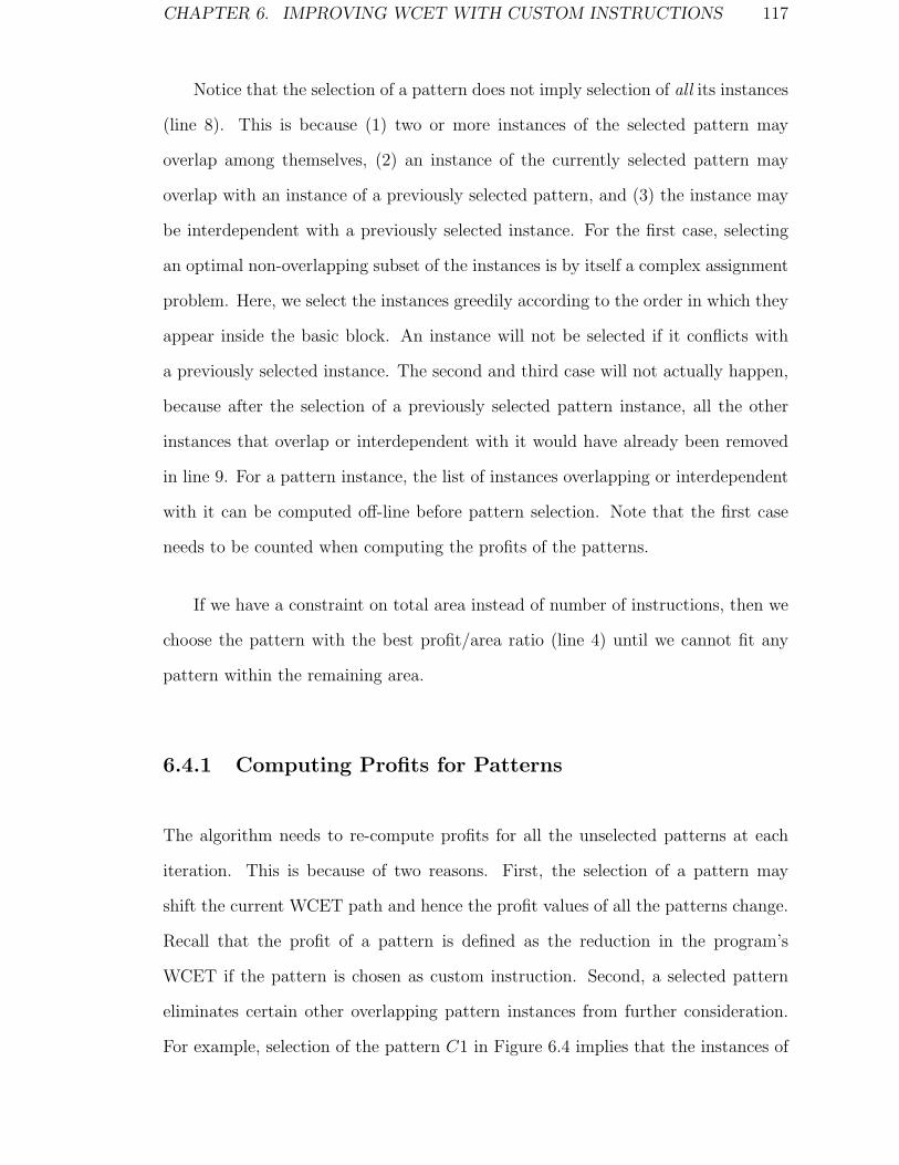
CHAPTER 6. IMPROVING WCET WITH CUSTOM INSTRUCTIONS 117
Notice that the selection of a pattern does not imply selection of all its instances
(line 8). This is because (1) two or more instances of the selected pattern may
overlap among themselves, (2) an instance of the currently selected pattern may
overlap with an instance of a previously selected pattern, and (3) the instance may
be interdependent with a previously selected instance. For the first case, selecting
an optimal non-overlapping subset of the instances is by itself a complex assignment
problem. Here, we select the instances greedily according to the order in which they
appear inside the basic block. An instance will not be selected if it conflicts with
a previously selected instance. The second and third case will not actually happen,
because after the selection of a previously selected pattern instance, all the other
instances that overlap or interdependent with it would have already been removed
in line 9. For a pattern instance, the list of instances overlapping or interdependent
with it can be computed off-line before pattern selection. Note that the first case
needs to be counted when computing the profits of the patterns.
If we have a constraint on total area instead of number of instructions, then we
choose the pattern with the best profit/area ratio (line 4) until we cannot fit any
pattern within the remaining area.
6.4.1 Computing Profits for Patterns
The algorithm needs to re-compute profits for all the unselected patterns at each
iteration. This is because of two reasons. First, the selection of a pattern may
shift the current WCET path and hence the profit values of all the patterns change.
Recall that the profit of a pattern is defined as the reduction in the program’s
WCET if the pattern is chosen as custom instruction. Second, a selected pattern
eliminates certain other overlapping pattern instances from further consideration.
For example, selection of the pattern C1 in Figure 6.4 implies that the instances of
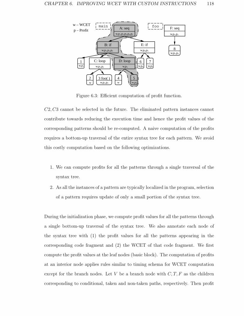
CHAPTER 6. IMPROVING WCET WITH CUSTOM INSTRUCTIONS 118
1, 47 {C1}
{ c11,c12,c13 }
m=0, prevW=50prevCset={φ} prevcset={φ}
1, 48 {C2} { c21 }
2, 46 {C2, C1}
{ c21,c12,c13 }
2, 46 {C2, C3} { c21,c31 }
3, 45 {C2, C3, C1} { c11,c31,c12 }
1, 47 {C1}
{ c11,c12,c13 }
m=0, prevW=50 prevCset={φ} prevcset={φ}
1, 48 {C2} { c21}
2, 46 {C2, C1}
{ c21,c11,c12 }
A: seq
54 2
1 6
B: if E: if
C: loop D: loop w,p1
3 foo( ) w,p1,p2 w,p3
w,p4w,p3w,p1,p2
w,p1,p2,p3 w,p4,p5
w,p1,p2,p3,p4,p5
7w,p5
w w
F: seq w,p1,p2
8 w,p1,p2
main foo w – WCET p – Profit
Figure 6.3: Efficient computation of profit function.
C2, C3 cannot be selected in the future. The eliminated pattern instances cannot
contribute towards reducing the execution time and hence the profit values of the
corresponding patterns should be re-computed. A naive computation of the profits
requires a bottom-up traversal of the entire syntax tree for each pattern. We avoid
this costly computation based on the following optimizations.
1. We can compute profits for all the patterns through a single traversal of the
syntax tree.
2. As all the instances of a pattern are typically localized in the program, selection
of a pattern requires update of only a small portion of the syntax tree.
During the initialization phase, we compute profit values for all the patterns through
a single bottom-up traversal of the syntax tree. We also annotate each node of
the syntax tree with (1) the profit values for all the patterns appearing in the
corresponding code fragment and (2) the WCET of that code fragment. We first
compute the profit values at the leaf nodes (basic block). The computation of profits
at an interior node applies rules similar to timing schema for WCET computation
except for the branch nodes. Let V be a branch node with C, T, F as the children
corresponding to conditional, taken and non-taken paths, respectively. Then profit
CHAPTER 6. IMPROVING WCET WITH CUSTOM INSTRUCTIONS 119
of a pattern p at the branch node V is defined as
profit(p, V ) = wcet(V )− (wcet(C)− profit(p, C))−
max (wcet(T )− profit(p, T ), wcet(F )− profit(p, F ))
The root node is annotated with all the patterns in the program. As the instances
of a pattern are typically localized, number of patterns is quite small for most of the
interior nodes, as shown in Figure 6.3.
Once a pattern is chosen at an iteration, we focus to the leaf nodes (basic blocks)
in which its selected instances appear. In these leaf nodes, we re-compute the profits
for all the unselected patterns which have instances eliminated due to overlapping
or interdependence with the current selected instances. Changes in a leaf node are
propagated towards the root of the syntax tree. At a interior node, the profit values
of all the patterns annotated on it will be reevaluated. The only nodes that need
to be updated in this phase are the nodes that lie on the path from the root to a
modified leaf node. The shaded nodes in Figure 6.3 gives an example of updates
after the selection of pattern p3.
With this optimization, the complexity of the algorithm is bounded by O(M ×
|P | × D × A), where M is the number of patterns to be selected from a library of
|P | patterns, D is the height of the syntax tree and A is the maximum number of
instances of a pattern.
6.4.2 Improving the Heuristic
The greedy heuristic presented in the previous subsection runs pretty fast. Unfor-
tunately, it makes inferior choices in the presence of subsumed patterns. We define
p as a subsumed pattern of q if there exists at least one instance of pattern p that is
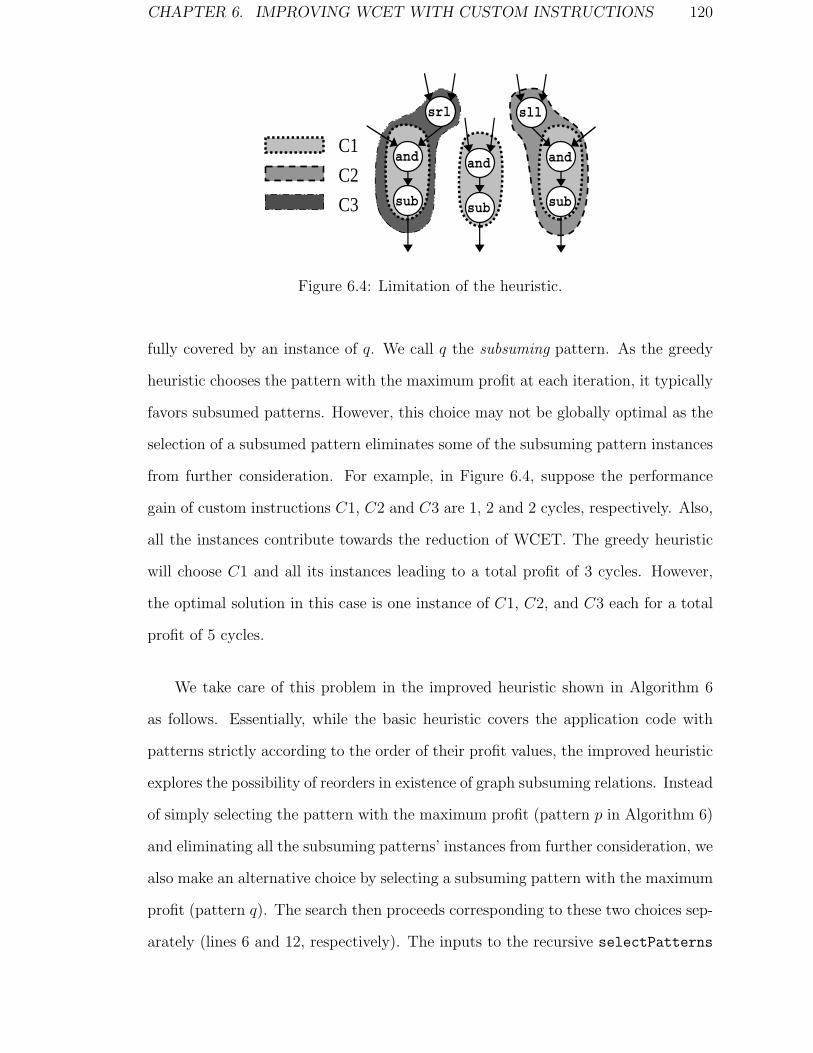
CHAPTER 6. IMPROVING WCET WITH CUSTOM INSTRUCTIONS 120
and
sub C3 C2 C1
and
sub
and
sub
sll
and
sub
and
sub
srlsll
and
sub
C3 C2 C1
and
sub
sll
and
sub
and
sub
srl
if branch
...
Same cycle
T F
sll srl
and
sub
sll
and
sub
and
sub C3C2C1
and
sub
and
sub
Figure 6.4: Limitation of the heuristic.
fully covered by an instance of q. We call q the subsuming pattern. As the greedy
heuristic chooses the pattern with the maximum profit at each iteration, it typically
favors subsumed patterns. However, this choice may not be globally optimal as the
selection of a subsumed pattern eliminates some of the subsuming pattern instances
from further consideration. For example, in Figure 6.4, suppose the performance
gain of custom instructions C1, C2 and C3 are 1, 2 and 2 cycles, respectively. Also,
all the instances contribute towards the reduction of WCET. The greedy heuristic
will choose C1 and all its instances leading to a total profit of 3 cycles. However,
the optimal solution in this case is one instance of C1, C2, and C3 each for a total
profit of 5 cycles.
We take care of this problem in the improved heuristic shown in Algorithm 6
as follows. Essentially, while the basic heuristic covers the application code with
patterns strictly according to the order of their profit values, the improved heuristic
explores the possibility of reorders in existence of graph subsuming relations. Instead
of simply selecting the pattern with the maximum profit (pattern p in Algorithm 6)
and eliminating all the subsuming patterns’ instances from further consideration, we
also make an alternative choice by selecting a subsuming pattern with the maximum
profit (pattern q). The search then proceeds corresponding to these two choices sep-
arately (lines 6 and 12, respectively). The inputs to the recursive selectPatterns

CHAPTER 6. IMPROVING WCET WITH CUSTOM INSTRUCTIONS 121
Algorithm 6: Improved Custom Instruction Selection Heuristic
selectPatterns(in)Input: in: partial selection of patterns, instances, and corresponding wcetOutput: complete selection of patterns, instances, and corresponding wcet
if in.m = M then return in;1
Let p ∈ (P − in.pat) be the pattern with max profit;2
if profit(p) = 0 then return in;3
Let ins(p) be the selected instances of pattern p;4
tmp.m := m+ 1; tmp.wcet := in.wcet− profit(p); tmp.pat := in.pat ∪ p;5
tmp.ins := in.ins ∪ ins(p);choice1 := selectPatterns (tmp);6
if subsuming(p)− in.pat = φ then return choice1;7
Let q ∈ subsuming(p)− in.pat be the pattern with max profit;8
if profit(q) = 0 then return choice1;9
Let ins(q) be the selected instances of pattern q;10
tmp.m := m+ 1; tmp.wcet := in.wcet− profit(q); tmp.pat := in.pat ∪ q;11
tmp.ins := in.ins ∪ ins(q);choice2 := selectPatterns (tmp);12
if choice1.wcet ≤ choice2.wcet then return choice1;13
else return choice2;
function are the patterns and instances selected so far and the corresponding WCET.
The function returns with the complete selection of up to M patterns. Finally, the
WCET corresponding to the two choices are compared (line 13) and the better one
is selected.
There are two more things to be noted. First, for the recursive selectPatterns
at line 6 (or line 12), because it assumes pattern p (or q) is selected, instances of
other patterns that are overlapping or interdependent with instances of p (or q)
should be excluded. Second, instead of exploring any subsuming case with possibly
little profit, we can impose a threshold, such as a certain percentage of p’s profit,
to the profit of the subsuming subgraph q. Only when q’s profit is greater than
the threshold, the other choice will be explored. This helps to constrain the run
time explosion at some cost of optima, depending on the threshold. However, in our
experiments, we do not impose such a threshold, since all test cases returns quickly
with the improved heuristic. The results show that this simple modification reduces
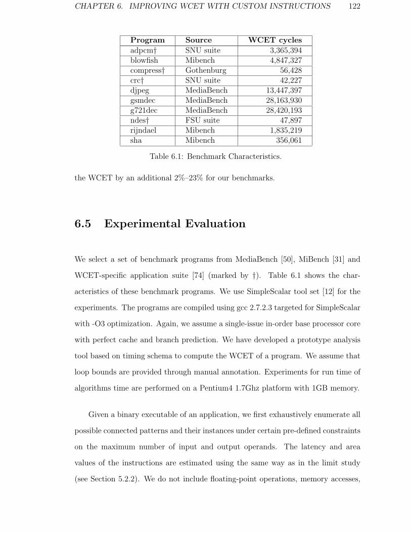
CHAPTER 6. IMPROVING WCET WITH CUSTOM INSTRUCTIONS 122
Program Source WCET cycles
adpcm† SNU suite 3,365,394blowfish Mibench 4,847,327compress† Gothenburg 56,428crc† SNU suite 42,227djpeg MediaBench 13,447,397gsmdec MediaBench 28,163,930g721dec MediaBench 28,420,193ndes† FSU suite 47,897rijndael Mibench 1,835,219sha Mibench 356,061
Table 6.1: Benchmark Characteristics.
the WCET by an additional 2%–23% for our benchmarks.
6.5 Experimental Evaluation
We select a set of benchmark programs from MediaBench [50], MiBench [31] and
WCET-specific application suite [74] (marked by †). Table 6.1 shows the char-
acteristics of these benchmark programs. We use SimpleScalar tool set [12] for the
experiments. The programs are compiled using gcc 2.7.2.3 targeted for SimpleScalar
with -O3 optimization. Again, we assume a single-issue in-order base processor core
with perfect cache and branch prediction. We have developed a prototype analysis
tool based on timing schema to compute the WCET of a program. We assume that
loop bounds are provided through manual annotation. Experiments for run time of
algorithms time are performed on a Pentium4 1.7Ghz platform with 1GB memory.
Given a binary executable of an application, we first exhaustively enumerate all
possible connected patterns and their instances under certain pre-defined constraints
on the maximum number of input and output operands. The latency and area
values of the instructions are estimated using the same way as in the limit study
(see Section 5.2.2). We do not include floating-point operations, memory accesses,

CHAPTER 6. IMPROVING WCET WITH CUSTOM INSTRUCTIONS 123
and conditional branches in custom instructions as they introduce non-deterministic
behavior.
We use ILOG CPLEX (v9.1) to obtain the optimal solutions for the ILP for-
mulations. lp solve, a popular public domain linear programming solver, fails to
terminate within reasonable time for most problem. We compute WCET reduction
as follows:
Reduction =Original WCET −Reduced WCET
Original WCET× 100%
We perform the custom instruction selection under a variety of scenarios in or-
der to stress our heuristic algorithm. The number of patterns and instances has
direct impact on the time required to solve the optimization problem. We control
the number of patterns generated for a benchmark by imposing different constraints
on the number of input and output operands allowed for a pattern. First, we con-
sider a constrained topology that allows at most 2 register inputs, 1 immediate input
and 1 register output for each custom instruction. This is realistic for most mod-
ern processors without major impact on their ISA format and micro-architecture.
Second, we consider a more aggressive relaxed topology that allows at most 4 inputs
(either register or immediate value) and 2 outputs. The relaxed topology results in
significantly more number of patterns and instances compared to the constrained
topology.
Table 6.2 and Table 6.3 show the WCET reduction if we can implement at
most 5 custom instructions under constrained and relaxed topology, respectively.
We confirm that custom instructions can indeed reduce the WCET of a program
significantly and make it easier for a real-time task to meet its deadline. Even with
constrained topology and a limit of only 5 custom instructions, we can still achieve
up to 22% reduction in worst case execution time. Allowing relaxed topology obtains

CHAPTER 6. IMPROVING WCET WITH CUSTOM INSTRUCTIONS 124
Program No. No. WCET Red. Run Time (s)Pat. Inst. Heur Opt. Heur Opt.
adpcm 51 150 9% 9% 0.002 0.02blowfish 15 276 16% 16% 0.002 0.02compress 37 92 2% 2% 0.002 0.01crc 12 23 15% 15% 0.001 0.01djpeg 64 485 7% 7% 0.017 0.12gsmdec 158 2312 21% 22% 0.031 0.10g721dec 73 180 4% 4% 0.006 0.03ndes 22 77 10% 10% 0.002 0.12rijndael 49 2520 16% 16% 0.034 1.25sha 9 40 12% 12% 0.001 0.01
Table 6.2: WCET Reduction under 5 custom instruction constraint with constrainedtopology.
Program No. No. WCET Red. Run Time (s)Pat. Inst. Heur Opt. Heur Opt.
adpcm 101 258 14% 14% 0.005 0.04blowfish 56 1221 39% 39% 0.012 11.1compress 141 248 6% 6% 0.003 0.02crc 24 39 17% 17% 0.001 0.01djpeg 226 1056 11% 11% 0.028 0.30gsmdec 796 6782 26% 26% 0.064 0.28g721dec 220 392 11% 11% 0.010 0.05ndes 77 182 17% 18% 0.003 0.03rijndael 156 9032 39% 39% 0.096 943sha 47 148 31% 31% 0.002 0.04
Table 6.3: WCET Reduction under 5 custom instruction constraint with relaxedtopology.
further reduction of WCET.
We also note that our improved heuristic (Heur in the Tables) obtains close to
the optimal results at a fraction of the ILP (Opt.) solving time. A comparison of the
Time column in Table 6.2 and Table 6.3 shows that the heuristic is quite scalable
as we increase the problem size; but ILP is not. For example, ILP solution time
increases from 1.25 sec to 943 seconds for the rijndael benchmark as we increase the
number of patterns. In fact, with even more relaxed topology constraint, there are a
few cases that CPLEX ILP solver cannot solve even after 24 hours. The heuristics
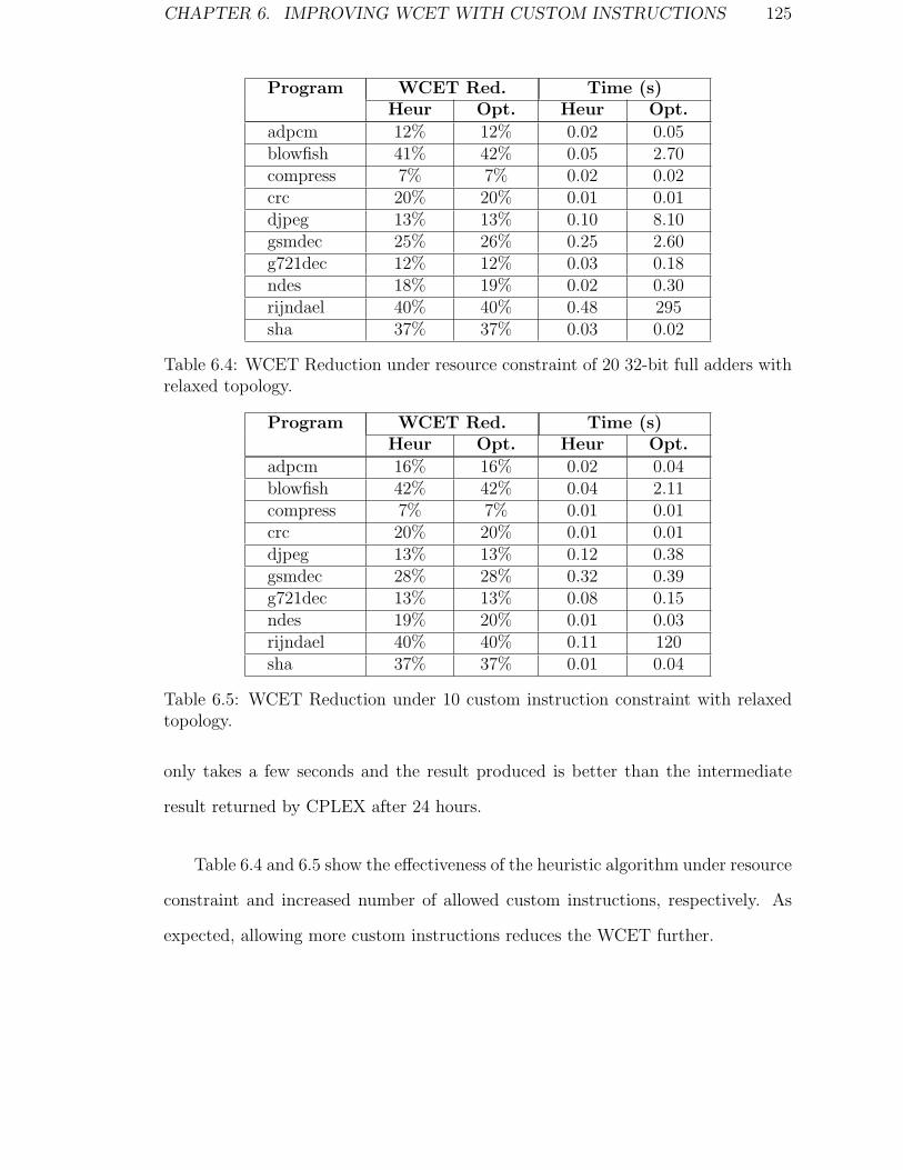
CHAPTER 6. IMPROVING WCET WITH CUSTOM INSTRUCTIONS 125
Program WCET Red. Time (s)Heur Opt. Heur Opt.
adpcm 12% 12% 0.02 0.05blowfish 41% 42% 0.05 2.70compress 7% 7% 0.02 0.02crc 20% 20% 0.01 0.01djpeg 13% 13% 0.10 8.10gsmdec 25% 26% 0.25 2.60g721dec 12% 12% 0.03 0.18ndes 18% 19% 0.02 0.30rijndael 40% 40% 0.48 295sha 37% 37% 0.03 0.02
Table 6.4: WCET Reduction under resource constraint of 20 32-bit full adders withrelaxed topology.
Program WCET Red. Time (s)Heur Opt. Heur Opt.
adpcm 16% 16% 0.02 0.04blowfish 42% 42% 0.04 2.11compress 7% 7% 0.01 0.01crc 20% 20% 0.01 0.01djpeg 13% 13% 0.12 0.38gsmdec 28% 28% 0.32 0.39g721dec 13% 13% 0.08 0.15ndes 19% 20% 0.01 0.03rijndael 40% 40% 0.11 120sha 37% 37% 0.01 0.04
Table 6.5: WCET Reduction under 10 custom instruction constraint with relaxedtopology.
only takes a few seconds and the result produced is better than the intermediate
result returned by CPLEX after 24 hours.
Table 6.4 and 6.5 show the effectiveness of the heuristic algorithm under resource
constraint and increased number of allowed custom instructions, respectively. As
expected, allowing more custom instructions reduces the WCET further.

CHAPTER 6. IMPROVING WCET WITH CUSTOM INSTRUCTIONS 126
6.6 Summary
We have introduced methodologies for using custom instructions to reduce the worst-
case execution time for real-time embedded systems. Other than increasing the
processor’s clock frequency or changing the software’s algorithm significantly, ISEP
provides another choice to meet timing constraints for real-time tasks.
The heuristic of custom instruction selection is based on pattern reuse, where
the potential of exhaustive enumeration of candidate subgraphs are explored. It
can be easily modified to adapt to normal custom instruction selection problem to
improve the average case execution, by replacing the profit function of a pattern
template with its average case cycle reduction.

Chapter 7
Conclusions
If people never did silly things, nothing intelligent would ever get done.
– Ludwig Wittgenstein
In this thesis, we have presented efficient methodologies for the optimal identifi-
cation of custom instructions. To this end, we exhaustively enumerate all the feasi-
ble subgraphs of relaxed topology, and then select the optimal subset under various
design constraints. Based on exhaustive enumeration, where all the isomorphic sub-
graphs can be exposed, custom instruction selection optimizes the performance by
maximizing the reuse of custom instructions. Both our enumeration algorithms and
selection methodologies are scalable and can be applied to applications with very
large DFGs especially resulting from modern compiler transformations for more in-
struction level parallelism. As a practical application, methodologies of using custom
instruction to improve the worst-case execution time to meet tight timing constraint
of real-time applications are also presented.
We discuss two other possible directions to explore for the software-hardware
partitioning problem of extensible processors in the future. First, while we consider
extensible processors for embedded applications, they are also great candidates for
127

CHAPTER 7. CONCLUSIONS 128
desktop and other high-end computations under superscalar/VLIW processor model.
In this context, optimal covering of the code with custom instructions may not yield
the best performance improvement. The selection algorithm need to work together
with the instruction scheduler to reduce the critical scheduling paths. Second, there
exists opportunities to cross optimize the CFUs to reduce the combined area such
that more custom instructions can be packed under tight area budget. Side effects
of latency increases for individual custom instructions need to be considered at the
same time in the selection process.
We envision that hardware-software interlaced custom architectures will set the
trend for future computing devices. With maturing automated design techniques,
performance and design flexibility are no longer unachievable at the same time.
The compiler for software design, and the high-level synthesis tools for hardware
design, previously holding two diverse philosophies (compute-in-time and compute-
in-space respectively) will finally merge. Under a unified framework, instruction
level customizable extensible processors would work with function level customizable
components to meet challenging design requirements.

Index
2-3 tree, 74
ACET – average case execution time, 109
ASIC — application-specific integrated cir-
cuit, 5
ASIP — application specific instruction-set
processor, 9
Bit vector, 74
BTB – branch target buffer, 32
CCA, 31
CFG – control flow graph, 18
CFU — custom functional unit, 14
Chimaera, 30
CISC — complex instruction-set computer,
8
Code motion, 39
Compiler, 17
Connected MIMO, 54
Connected pattern set, 69
Connectivity, 44
Control localization, 40
Convexity, 55
Custom instruction, 14
Custom instruction identification, 16
Custom instruction instance, 19, 88
DAG – directed acyclic graph, 98
DFG – dataflow graph, 18, 52
DISC, 25
Disjoint MIMO, 54
downCone – downward cone, 54
DPS – Disjoint pattern set, 69
DSP — digital signal processor, 8
Embedded System, 1
Feasibility of pattern, 55
FPGA — field-programmable gate array, 11
FU — functional units, 3
Garp, 26
GPP — general purpose processor, 3
Hardware, 5, 7
Hardware-Software partitioning, 16
ILP – instruction level parallelism, 38
Interdependent subgraphs, 89
Invalid node, 53
IR – intermediate representation, 18
ISA — instruction set architecture, 3
ISE — instruction-set extension, 14
ISEP — instruction-set extensible proces-
sor, 14
129
INDEX 130
Isomorphism, 88
Logic block, 11
LUT — lookup table, 12
MAC — multiply-accumulate, 8
MIMO – multiple input multiple output, 44
MISO – multiple input single output, 43, 54
NRE — non-recurring engineering, 6
Overlap, 45
Partial decomposition, 61
Partial evaluation, 14
Pattern, 53
PEAS, 33
Predicated execution, 39
PRISC, 28
Reconfigurable Computing, 11
Region, 53
RISC — reduced instruction-set computer,
8
SIMD — single instruction, multiple data, 8
Software, 3, 7
Specialization, 2
SRAM — static random access memory, 12
Subsumed pattern, 119
Subsuming pattern, 120
Superscalar architecture, 4
Template pattern, 19, 88
Timing schema, 112
upCone – upward cone, 54
Upward scope, 71
Valid node, 53
VLIW — very long instruction word archi-
tecture, 4
WCET – worst case execution time, 110
WPP – whole program path, 96

Bibliography
[1] 3DSP. Sp-5flex dsp core. http://www.3dsp.com/sp5_flex.shtml/.
[2] A. Aho, M. Ganapathi, and S. W. K. Tjiang. Code generation using tree match-
ing and dynamic programming. ACM Transactions on Programming Language
and Systems (TOPLAS), 11(4), 1989.
[3] A. Aho, J. Hopcroft, and J. Ullman. Data structures and Algorithms. Addison-
Wesley, 1987.
[4] Altera. Nios embedded processor system development. http://www.altera.
com/products/ip/processors/nios/nio-index.html.
[5] M. Arnold. Instruction set extension for embedded processors. PhD thesis, Delft
University of Technology, 2001.
[6] M. Arnold and H. Corporaal. Designing domain-specific processors. In The 9th
International Symposium on Hardware/Software Codesign (CODES), 2001.
[7] K. Atasu, G. Dundar, and C. Ozturan. An integer linear programming ap-
proach for identifying instruction-set extensions. In International Conference
on Hardware/Software Codesign and System Synthesis (CODES+ISSS), 2005.
[8] K. Atasu, L. Pozzi, and P. Ienne. Automatic application-specific instruction-set
extensions under microarchitectural constraints. In Design Automation Con-
ference (DAC), 2003.
131

BIBLIOGRAPHY 132
[9] M. Baleani, F. Gennari, Y. Jiang, Y. Patel, R. K. Brayton, and A. Sangiovanni-
Vincentelli. HW/SW partitioning and code generation of embedded control ap-
plications on a reconfigurable architecture platform. In The 10th International
symposium on Hardware/Software Codesign (CODES), May 2002.
[10] J. E. Bennett. A methodolgy of automated design of computer instruction sets.
PhD thesis, University of Cambridge, Computer laboratory, 1988.
[11] P. Brisk, A. Kaplan, R. Kastner, and M. Sarrafzadeh. Instruction genera-
tion and regularity extraction for reconfigurable processors. In International
Conference on Compilers, Architectures, and Synthesis for Embedded Systems
(CASES), October 2002.
[12] D. Burger, T. Austin, and S. Bennett. Evaluating future microprocessors: the
SimpleScalar toolset. In Technical Report CS-TR96-1308. Univ. of Wisconsin
- Madison, 1996. Available from http://www.simplescalar.com.
[13] T. J. Callahan and J. Wawrzynek. Instruction-level parallelism for reconfig-
urable computing. In Proceedings of the 8th International Workshop on Field-
Programmable Logic and Applications, From FPGAs to Computing Paradigm,
1998.
[14] J. M. P. Cardoso and M. P. Vestias. Architectures and compilers to support
reconfigurable computing. ACM Crossroads, 5(3):15–22, 1999.
[15] B. Chakraborty, T. Chen, T. Mitra, and A. Roychoudhury. Handling constraints
in multi-objective GA for embedded system design. In International Conference
on VLSI Design: VLSI in Mobile Communication (VLSID), 2006.
[16] L. N. Chakrapani, J. Gyllenhaal, W. W. Hwu, S. A. Mahlke, K. V. Palem, and
R. M. Rabbah. Trimaran, an infrastructure for research in instruction level
parallelism. In International Workshop on Languages and Compilers for High
Performance Computing (LCPC), 2004.

BIBLIOGRAPHY 133
[17] X. Chen, D. L. Maskell, and Y. Sun. Fast identification of custom instructions
for extensible processors. IEEE Transactions on Computer-Aided Design of
Integrated Circuits and Systems (TCAD), 26(2), 2007.
[18] N. Cheung, S. Parameswaran, and J. Henkel. INSIDE: Instruction selec-
tion/identification & design exploration for extensible processors. In Inter-
national Conference on Computer Aided Design (ICCAD), 2002.
[19] H. Choi, J. S. Kim, C. W. Yoon, I. C. Park, S. H. Hwang, and C. M. Kyung.
Synthesis of application specific instructions for embedded DSP software. IEEE
Transactions on Computers, 48(6), June 1999.
[20] N. Clark, J. Blome, M. Chu, S. Mahlke, S. Biles, and K. Flautner. An archi-
tecture framework for transparent instruction set customization in embedded
processors. In International Symposium on Computer Architecture (ISCA),
2005.
[21] N. Clark, M. Kudlur, H. Park, S. Mahlke, and K. Flautner. Application-specific
processing on a general-purpose core via transparent instruction set customiza-
tion. In Annual IEEE/ACM International Symposium on Microarchitecture
(MICRO), 2004.
[22] N. Clark, H. Zhong, and S. Mahlke. Processor acceleration through automated
instruction set customization. In Annual IEEE/ACM International Symposium
on Microarchitecture (MICRO), 2003.
[23] K. Compton and S. Hauck. Configurable computing: A survey of systems and
software. ACM Computing Surveys, 34(2):171–210, June 2002.
[24] J. Cong, Y. Fan, G. Han, A. Jagannathan, G. Reinman, and Z. Zhang. In-
struction set extension with shadow registers for configurable processors. In
International Symposium on Field Programmable Gate Arrays (FPGA), 2005.
BIBLIOGRAPHY 134
[25] J. Cong, Y. Fan, G. Han, and Z. Zhang. Application-specific instruction gener-
ation for configurable processor architectures. In International Symposium on
Field Programmable Gate Arrays (FPGA), 2004.
[26] CoWare. Coware processor designer. http://www.coware.com/products/
processordesigner.php/.
[27] J. A. Fisher. Trace scheduling: A technique for global microcode compaction.
IEEE Transactions on Computers, 30(9):478–490, July 1981.
[28] C. Galuzzi, E. Moscu Panainte, Y.D. Yankova, K.L.M. Bertels, and S. Vassil-
iadis. Automatic selection of application-specific instruction-set extensions. In
International Conference on Hardware/Software Codesign and System Synthe-
sis (CODES+ISSS), 2006.
[29] R. E. Gonzalez. Xtensa: A configurable and extensible processor. Annual
IEEE/ACM International Symposium on Microarchitecture (MICRO), 20(2),
2000.
[30] D. Goodwin and D. Petkov. Automatic generation of application specific pro-
cessors. In International Conference on Compilers, Architectures, and Synthesis
for Embedded Systems (CASES), 2003.
[31] M. R. Guthaus, J. S. Ringenberg, D. Ernst, T. M. Austin, T. Mudge, and R. B.
Brown. Mibench: A free, commercially representative embedded benchmark.
In IEEE 4th Annual Workshop on Workload Characterization (WWC), 2001.
Benchmark available from http://www.eecs.umich.edu/mibench/.
[32] P. K. Hanumolu. Design techniques for clocking high performance signaling
systems. PhD thesis, Oregon State University, 2006.
[33] S. Hauck, T. W. Fry, M. M. Hosler, and J. P. Kao. The Chimaera reconfigurable
functional unit. IEEE Transactions on VLSI Systems, 12, 2004.

BIBLIOGRAPHY 135
[34] J. R. Hauser and J. Wawrzynek. Garp: A MIPS processor with a reconfigurable
coprocessor. In IEEE Symposium on Field-Programmable Custom Computing
Machines (FCCM), April 1997.
[35] B. Holmer. Automatic design of computer instruction sets. PhD thesis, Uni-
versity of California, Berkeley, 1993.
[36] P. Y T Hsu and E. S. Davidson. Highly concurrent scalar processing. ACM
SIGARCH Computer Architecture News, 14(2), 1986.
[37] I. Huang and A. M. Despain. Synthesis of application specific instruction sets.
IEEE Transactions on Computer-Aided Design of Integrated Circuits and Sys-
tems (TCAD), 14(6), June 1995.
[38] W. W. Hwu, S. A. Mahlke, W. Y. Chen, P. P. Chang, N. J. Water, R. A.
Bringmann, R. G. Ouellette, R. E. Hank, T. Kiyohara, G. E. Haab, J. G.
Holm, and D. M. Lavery. The superblock: An effective structure for VLIW and
superscalar compilation. Journal of Supercomputing, 7, 1993.
[39] Altera Inc. Altera devices. http://www.altera.com/products/devices/.
[40] Synopsys Inc. DesignWare library datapath and building block IP. http:
//www.synopsys.com/dw/buildingblock.php.
[41] Xilinx Inc. Virtex-5 multi-platform FPGA. http://www.xilinx.com/virtex5.
[42] R. Jayaseelan, H. Liu, and T. Mitra. Exploiting forwarding to improve data
bandwidth of instruction-set extensions. In Design Automation Conference
(DAC), 2006.
[43] R. Kastner, A. Kaplan, S. Ogrenci Memik, and E. Bozorgzadeh. Instruction
generation for hybrid reconfigurable systems. ACM Transactions on Design
Automation of Electronic Systems (TODAES), 7(4):605–627, October 2002.

BIBLIOGRAPHY 136
[44] B. Kastrup. Automatic synthesis of reconfigurable instruction set accelerators.
PhD thesis, Philips Research, 2001.
[45] K. Kennedy and K. S. McKinley. Maximizing loop parallelism and improving
data locality via loop fusion and distribution. In Workshop on Languages and
Compilers for Parallel Computing (LCPC), Portland, Ore., 1993.
[46] A. Kitajima, M. Itoh, J. Sato, A. Shiomi, Y. Takeuchi, and M. Imai. Effective-
ness of the ASIP design system PEAS-III in design of pipelined processors. In
Asia and South Pacific Design Automation Conference (ASPDAC), 2001.
[47] K. Kucukcakar. An ASIP design methodology for embedded systems. In The
7th International Workshop on Hardware/Software Codesign (CODES), 1999.
[48] J. R. Larus. Whole program paths. In ACM International Conference on
Programming Language Design and Implementation (PLDI), 1999.
[49] L. Lavagno, A. La Rosa, and C. Passerone. Hardware/software design space
exploration for a reconfigurable processor. In Design, Automation and Test in
Europe (DATE), 2003.
[50] C. Lee, M. Potkonjak, and W. H. Mangione-Smith. Mediabench: a tool for
evaluating and synthesizing multimedia and communicatons systems. In Annual
IEEE/ACM International Symposium on Microarchitecture (MICRO), 1997.
[51] J. Lee, K. Choi, and N. Dutt. Efficient instruction encoding for automatic
instruction set design of configurable ASIPs. In International Conference on
Computer Aided Design (ICCAD), 2002.
[52] J. S. Lee, Y. S. Jeon, and M. H. Sunwoo. Design of new DSP instructions and
their hardware architecture for high-speed FFT. In IEEE workshop on signal
processing systems (SiPS), 2001.

BIBLIOGRAPHY 137
[53] S. Lee et al. A flexible tradeoff between code size and WCET using a dual
instruction set processor. In International Workshop on Software and Compilers
for Embedded Systems (SCOPES), 2004.
[54] W. Lee, R. Barua, M. Frank, D. Srikrishna, J. Babb, V. Sarkar, and S. Amaras-
inghe. Space-time scheduling of instruction-level parallelism on a raw machine.
In Architectural Support for Programming Languages and Operating Systems
(ASPLOS), pages 46–57, 1998.
[55] R. Leupers, K. Karuri, S. Kraemer, and M. Pandey. A design flow for con-
figurable embedded processors based on optimized instruction set extension
synthesis. In Design, Automation and Test in Europe (DATE), 2006.
[56] S. Liao, S. Devadas, K. Keutzer, and S. Tjiang. Instruction selection using
binate covering for code size optimization. In International Conference on
Computer Aided Design (ICCAD), 1995.
[57] C. Liem, T. May, and P. Paulin. Instruction-set matching and selection for DSP
and ASIP code generation. In European Design and Test Conference (EDTC),
1994.
[58] S. A. Mahlke, D. C. Lin, W. Y. Chen, R. E. Hank, and R. A. Bringmann.
Effective compiler support for predicated execution using the hyperblock. In
Annual IEEE/ACM International Symposium on Microarchitecture (MICRO),
1992.
[59] N. Manning and I. Witten. Sequitur source code. http://sequitur.info.
[60] C. Nevill-Manning and I. Witte. Identifying hierarchical structure in sequences:
A linear-time algorithm. Journal of Artificial Intelligence Research, 7, 1997.

BIBLIOGRAPHY 138
[61] T. Okuma, H. Tomiyama, A. Inoue, E. Fajar, and H. Yasuura. Instruction
encoding techniques for area minimization of instruction ROM. In International
Symposium on System Synthesis (ISSS), 1998.
[62] S. Palacharla, N. P. Jouppi, and J. E. Smith. Complexity-effective superscalar
processors. In International Symposium on Computer Architecture (ISCA),
1997.
[63] C. Y. Park and A. C. Shaw. Experiments with a program timing tool based on
source-level timing schema. IEEE Computer, 24(5), 1991.
[64] G. Pospischil et al. Developing real-time tasks with predictable timing. IEEE
Software, 9(5), 1992.
[65] L. Pozzi. Methodologies for the design of application-specific reconfigurable
VLIW processors. PhD thesis, Politecnico Di Milano, 2000.
[66] L. Pozzi, K. Atasu, and P. Ienne. Exact and approximate algorithms
for the extension of embedded processor instruction sets. IEEE Transac-
tions on Computer-Aided Design of Integrated Circuits and Systems (TCAD),
25(7):1209–29, July 2006.
[67] L. Pozzi, M. Vuletic, and P. Ienne. Automatic topology-based identification of
instruction-set extensions for embedded processor. In Technical Report 01/377.
Swiss Federal Institute of Technology Lausanne (EPFL), 2001.
[68] S. Radhakrishnan, Hui Guo, S. Parameswaran, and A. Ignjatovic. Application
specific forwarding network and instruction encoding for multi-pipe ASIPs. In
International Conference on Hardware/Software Codesign and System Synthe-
sis (CODES+ISSS), 2006.
[69] B. R. Rau and M. S. Schlansker. Embedded computer architecture and au-
tomation. Computer, 34(4):75–81, April 2001.

BIBLIOGRAPHY 139
[70] R. Razdan and M.D. Smith. A high-performance microarchitecture with
hardware-programmable functional units. In Annual IEEE/ACM International
Symposium on Microarchitecture (MICRO), 1994.
[71] J. Sato, A. Y. Alomary, Y. Honma, T. Nakata, A. Shiomi, N. Hikichi, and
M. Imai. PEAS-I: A hardware/software codesign system for ASIP development.
Transactions on Fundamentals of Electronics, Communications and Computer
Sciences (IEICE), March 1994.
[72] H. Scharwaechter, D. Kammler, A. Wieferink, M. Hohenauer, K. Karuri,
J. Ceng, R. Leupers, G. Ascheid, and H. Meyr. ASIP architecture exploration
for efficient IPSec encryption: A case study. ACM Transactions on Embedded
Computing Systems (TECS), 6(2):12, 2007.
[73] J. Shu, T. C. Wilson, and D. K. Banerji. Instruction-set matching and GA-based
selection for embedded-processor code generation. In International Conference
on VLSI Design: VLSI in Mobile Communication (VLSID), 1996.
[74] F. Stappert. WCET benchmarks. Available from http://www.c-lab.de/
home/en/download.html.
[75] Stretch inc. Stretch S5000 Product Brief. http://www.stretchinc.com/
products_s5000.php.
[76] V. Suhendra, T. Mitra, A. Roychoudhury, and T. Chen. WCET centric data al-
location to scratchpad memory. In The Real-Time Systems Symposium (RTSS),
2005.
[77] F. Sun, S. Ravi, A. Raghunathan, and N.K.Jha. Custom-instruction synthe-
sis for extensible-processor platforms. IEEE Transactions on Computer-Aided
Design of Integrated Circuits and Systems (TCAD), 23(2), 2004.

BIBLIOGRAPHY 140
[78] E. Talpes and D. Marculescu. Increased scalability and power efficiency by using
multiple speed pipelines. In International Symposium on Computer Architecture
(ISCA), 2005.
[79] Tensilica, Inc. Tensilica instruction extension language, user’s guide. Issue
date: 11/2006.
[80] Trimaran. Trimaran Documentation. Avaliable from http://www.trimaran.
org/documentation.shtml.
[81] M. J. Wirthlin and B. L. Hutchings. DISC: the dynamic instruction set com-
puter. In Field Programmable Gate Arrays (FPGAs) for Fast Board Develop-
ment and Reconfigurable Computing (SPIE), 1995.
[82] A. Ye, A. Moshovos, S. Hauck, and P. Banerjee. Chimaera: A high-performance
achitecture with a tightly-coupled reconfigurable functional unit. In Interna-
tional Symposium on Computer Architecture (ISCA), 2000.
[83] W. Zhao, W. Kreahling, D. Whalley, C. Healy, and F. Mueller. Improving
WCET by optimizing worst-case paths. In IEEE Real-Time and Embedded
Technology and Applications Symposium (RTAS), 2005.
[84] W. Zhao, P. Kulkarni, and D. Whalley. Tuning the WCET of embedded ap-
plications. In IEEE Real-Time and Embedded Technology and Applications
Symposium (RTAS), 2004.
[85] W. Zhao, D. Whalley, C. Healy, and F. Mueller. WCET code positioning. In
The Real-Time Systems Symposium (RTSS), 2004.

Appendix A
ISE Tool on Trimaran
To facilitate research on instruction-set extension for advanced processors, we de-
veloped an ISE module based on the Trimaran compiler infrastructure [16, 80]. Tri-
maran front-end is a C compiler equipped with a large suite of machine independent
optimizations. Internal transformations are based on its intermediate representation
graphs called Elcor. The back-end of the compiler performs instruction scheduling,
register allocation, machine dependent optimizations for the state-of-the-art VLIW
architecture. Finally, the executable is simulated with cycle accurate simulator for
performance evaluation and other run-time statistics.
Our ISE module is inserted as an extra phase of the Trimaran back-end right
before instruction scheduling and register allocation. The module is kept as in-
dependent as possible to the rest of the modules in Trimaran so that it can be
used elsewhere with little modification Custom instruction formation before register
allocation ensures that it is not hindered by false data dependencies (a.k.a., write-
after-read and write-after-write dependencies). Figure A.1 shows a case where a
pattern cannot be used as custom instruction due to WAR dependency introduced
by register allocation.
141

APPENDIX A. ISE TOOL ON TRIMARAN 142
1
2
3
R1 R2
R3R4
R6
R3
R5
Figure A.1: Pattern {1, 3} cannot be used without resolving WAR dependencybetween node 2 and 3 (caused by reusing register R3).
A.1 Work Flow
The work flow includes the following three steps.
Step 1: ISE generation — ISE enumeration and selection algorithms work together
to identify and select a set of optimized custom instructions;
Step 2: modify the target machine (Mdes in Trimaran) and compiler in order to
support the new ISE;
Step 3: ISE utilization - replace selected custom instructions in the application.
At the end of the 3rd step, the simulator should be able to execute the ISE
enabled version of the given application.
After the ISE generation step, the selected patterns cannot be directly replaced
with corresponding custom instructions. This is because the compiler for the old
architecture does not recognize the new custom instructions and is unable to assign
opcode for them; the simulator also has no idea how to execute them. After mod-
ifying the target machine architecture mainly by inserting descriptions of custom
instructions (format, semantics, various execution requirements and properties), we
recompile the compiler and simulator to reflect the changes. After that, custom

APPENDIX A. ISE TOOL ON TRIMARAN 143
Selected patternsand instances
G t C t i t ti Simulatable executableGenerate new compiler for ISE
Custom instructionreplacementISE Identification
Simulatable executablewith
custom instructions
Machine Descriptionfor new instructions
& setup files
Figure A.2: Work flow of ISE enabled compilation.
instruction replacement is taken place by the new compiler, followed by instruction
scheduling and register allocation. The produced executable with custom instruc-
tions can now be understood and simulated by the new simulator. A simple run of
the compilation flow is presented in Figure A.2.
In custom instruction replacement, a subgraph of multiple operations is replaced
with the single corresponding custom instruction. We have to take note of two
things here. First, the position of an input register or output register of the custom
instruction must match with that of its topologically equivalent register on the
custom instruction template (from which we defined the format and semantics of
the custom instruction). We use a procedure similar to the isomorphism check
to identify these correspondences and sort the order. Second, we must maintain
the partial order between the custom instruction and other instructions to ensure
correctness of the assembly code. Figure A.3 shows an example how the partial
order can be infringed due to the reduction of multiple operations to a single custom
instruction. As discussed in [22], if a successor (node 3 in Figure A.3) of the custom
instruction comes before the last predecessor of the custom instruction (node 4), the
successor along with any operations dependent on it should be reordered after the
last predecessor. The custom instruction is inserted after its last predecessor.

APPENDIX A. ISE TOOL ON TRIMARAN 144
1
2
3
4
5
6
1
x
3
4
(a) (b)
Figure A.3: Order of custom instruction insertion. (a) Original operations is topo-logically ordered correctly (adapted from [22]), (b) The partial order is broken (node4 and 3) after custom instruction replacement.
A.2 Limitations of the Tool
The current version of the ISE module is at the basic block level. Trimaran infras-
tructure supports various larger structures to exploit more instruction level paral-
lelism for the underlining VLIW architecture, such as trace, superblock and hyper-
block. When the ISE module is applied on trace and superblock level, the operations
of a selected custom instruction must be moved to a single basic block, with patch
code inserted (bookkeeping) to ensure the semantic correctness after code motion.
On hyperblock level with predicated execution support, predicate registers should
be counted for as input/output operands when identifying custom instructions.
Furthermore, due to restrictions of Trimaran instruction format, up to 4-input
and 4-output operands are allowed in a custom instruction. However, this is a
reasonable architectural restriction for processor realization. Our limit study in
Chapter 5 also suggests that going beyond these numbers only provides marginal
benefit. Lastly, only single source file benchmarks are supported currently. Trimaran
compilation is triggered separately on each source file (before the link stage), while
the selection of custom instructions concerning pattern reuse requires a global view
of the whole application.