DESIGN, MANUFACTURE AND TESTING OF A

Bend-Twist D-spar Cheng-Huat Ong & Stephen W. Tsai Department of Aeronautics &Astronautics Stanford University Stanford CA 94305-4035

-8

SAND99-1324 Unlimited Release Printed June 1999

@I Sandia National Laboratories

Issued by Sandia National Laboratories, operated for the United States Department of Energy by Sandia Corporation.

NOTICE: This report was prepared as an account of work sponsored by an agency of the United States Government. Neither the United States Government, nor any agency thereof, nor any of their employees, nor any of their contractors, subcontractors, or their employees, make any warranty, express or implied, or assume any legal liability or responsibility for the accuracy, completeness, or usefulness of any information, apparatus, product, or process disclosed, or represent that its use would not infringe privately owned rights. Reference herein to any specific commercial product, process, or service by trade name, trademark, manufacturer, or otherwise, does not necessarily constitute or imply its endorsement, recommendation, or favoring by the United States Government, any agency thereof, or any of their contractors or subcontractors. The views and opinions expressed herein do not necessarily state or reflect those of the United States Government, any agency thereof, or any of their contractors.

Printed in the United States of America. This report has been reproduced directly from the best available copy.

Available to DOE and DOE contractors from Office of Scientific and Technical Information P.O. Box 62 Oak Ridge, TN 37831

Prices available from (703) 605-6000 Web site: http://www.ntis.gov/ordering.htm

Available to the public from National Technical Information Service U.S. Department of Commerce 5285 Port Royal Rd Springfield, VA 22161

NTIS price codes Printed copy: A03 Microfiche copy: A01

i

SAND 99-1324Unlimited Distribution

Printed June 1999

Design, Manufacture and Testing of A Bend-Twist D-spar

Cheng-Huat Ong & Stephen W. Tsai

Department of Aeronautics & Astronautics

Stanford University

Stanford CA 94305-4035

Sandia Contract: BB-6066

Abstract

Studies have indicated that an adaptive wind turbine blade design cansignificantly enhance the performance of the wind turbine blade on energy capture andload mitigation. In order to realize the potential benefits of aeroelastic tailoring, a bend-twist D-spar, which is the backbone of a blade, was designed and fabricated to achievethe objectives of having maximum bend-twist coupling and fulfilling desirable structuralproperties (EI & GJ). Two bend-twist D-spars, a hybrid of glass and carbon fibers and anall-carbon D-spar, were fabricated using a bladder process. One of the D-spars, the hybridD-spar, was subjected to a cantilever static test and modal testing.

Various parameters such as materials, laminate schedule, thickness and internalrib were examined in designing a bend-twist D-spar. The fabrication tooling, the lay-upprocess and the joint design for two symmetric clamshells are described in this report.Finally, comparisons between the experimental test results and numerical results arepresented. The comparisons indicate that the numerical analysis (static and modalanalysis) agrees well with test results.

ii

Acknowledgements

This project was supported by Sandia National Laboratories under Contract No.BB-6066. The Technical Monitor is Dr. Paul S. Veers. The authors would like to thankDr. D. W. Lobitz and Dr. P. S. Veers for their participation in many beneficialdiscussions. The authors would like to thank Dr. Thomas G. Carne and his staff, fromSandia National Laboratories, for sharing his experience on modal testing and test data.The authors would also like to thank the staffs and researchers from Materials ResearchLaboratories/ Industrial Technology Research Institute (Taiwan) for their support andassistance in the fabrication and static testing of D-spars. The authors would like to thankMs. Julie Wang for her contribution and effort on D-spar fabrication and testing.

iii

Contents

1. Introduction 1

2. 3D-Beam Software Modifications & Verification 3

2.1 3D-Beam Modifications2.2 3D-Beam Verification

3. Parametric Study 15

3.1 Theoretical Estimation of the Coupling Coefficient, α3.2 Numerical Estimation of the Coupling Coefficient, α3.3 Summary

4. D-spar Design 44

4.1 D-spar Design Specification4.2 Theoretical Approach in Estimating Maximum Tip Rotation4.3 Numerical Estimation of Tip Rotation4.4 D-spar Structural Integrity4.5 D-spar Configurations for Demonstration

5. D-spar Fabrication 62

5.1 Tooling and Materials Used in D-spars Fabrication5.2 Fabrication Process5.3 Earlier Phase Fabrication Problems5.4 Staggered Overlap Joint Design

6. D-spar Static & Modal Testing 79

6.1 Static Test Set-up6.2 Static Test Results6.3 Comparison Between Estimated and Experimental Results6.4 Post Modal Test Analysis

7. Conclusions 104

References 105

1

Chapter 1

Introduction

Researchers are exploring the potential benefits of the anisotropic characteristicsof composite materials. A composite design that exhibits various degrees of anisotropyhas tremendous advantages not seen in an orthotropic composite structure. The benefitsare seen either in fixed wing, helicopter blade or wind turbine blade design.

One of the applications of aeroelastic tailoring is the use of a bend-twist coupledcomposite wing to prevent divergence of the forward swept wing.1 Weisshaar1 alsohighlighted other potential benefits for a fixed wing design, such as load relief, vibrationcontrol and increase of lift coefficients, resulting from the application of bend-twistcoupling.

Smith & Chopra2 proposed that composite designs exhibiting various couplingsappear to have great potential for use in helicopter blades and tilt-rotor blades to reducevibration, enhance aeroelastic stability, and improve aerodynamic efficiency. Theyformulated an analytical model for composite box-beam in the shape of a rectangle orsquare for rotor blade application. Their model can predict the behavior of a compositebox-beam that exhibits bend-twist or extension-twist coupling. Their analyticalpredictions agree generally well with the results of the finite element model (FEM) andthe experimental model.3 The highlight of their findings is that torsion-related out-of-plane warping can substantially influence torsion and coupled torsion deformations in asymmetric lay-up box-beam.

The application of elastic (or aeroelastic) tailoring can also be found in windturbine applications. Karaolis4, 5 demonstrates the concept of anisotropy lay-ups in bladeskin to achieve different types of twist coupling for wind turbine applications. Kooijman6

investigated the optimum bend-twist flexibility distribution of a rotor blade to improverotor blade design. Lobitz and Veers7 studied generic coupling effects on the annualenergy production of a stall-regulated wind turbine. They concluded that, with a smalltwist, a stall-controlled, fixed-pitch system could be operated with a larger rotor toachieve net energy enhancements.

Our interests here are related to the physical application of elastic tailoring ofcomposite materials to enhance load mitigation as studied by Lobitz and Laino8.Although there are potential benefits to elastic tailoring, there are key issues that need tobe resolved before the actual realization of a bend-twist coupled wind turbine blade. Twoof the key issues are dynamic stability and the ability to manufacture a bend-twist coupleblade. Lobitz and Veers9 address two of the most common stability constraints, namely,flutter and divergence. A coupling coefficient, α, is used to facilitate the genericexamination of the flutter and divergence boundary of a combined experiment blade(CEB). The study indicates that the flutter and divergence airspeeds are a function of thestrength of the coupling; the strength of the coupling increases as the magnitude of thecoupling coefficient, α, increases.

2

Mathematically, the range of α is between -1 and 1 as indicated by Lobitz andVeers.9 The implicit question that needs to be addressed is the feasible range of α ifcomposite materials are used. In the present study, an airfoil-type structure, a D-spar, isused as a test case to establish the achievable α range and the critical key parameters thatexhibit a higher degree of coupling. The D-spars were designed to meet specificdimensions, desirable structural properties, and the maximum bend-induced twist per unitpound. The ability to manufacture bend-twist coupled D-spars is also demonstrated.Finally, one of the D-spars was subjected to a cantilever static test and the test results arecompared to numerical results.

3

Chapter 2

3D-Beam Software Modifications & Verification

The 3D-Beam10 program is for analyzing composite beam and frame structureswith arbitrary cross-sections by the finite element method. The backbone of this programis a spreadsheet based software, Microsoft Excel. Therefore, the 3D-Beam is usable onany personal computer that runs the spreadsheet program.

This program is further modified to include the following features:

a. Option for "Plane Stress" input,

b. Option for "Thin Wall" input, and

c. Torsion-related Out-of-Plane warping for closed cell.

A series of cantilevered static tests (bending and torsion) has been conducted to verify the3D-Beam predictions. The types of beams tested consisted of aluminum boxes,orthotropic and anisotropic sandwich beams, and composite box beams.

2.1 3D-Beam Modifications

2.1.1 Option for "Plane Stress" input

One of the basic assumptions used in the formulation of 3D-Beam equations isthat the transverse strain (e2, see Figure 2.1 for the notation) is zero. This is a naturalconsequence of the one-dimensional nature of beam theory itself. Smith & Chopra2

stressed that when the walls of the box-beam are made of laminated composite materialplies, transverse in-plane normal stress and strain can be quite important. They furtherexamined three different methods for accounting for skin in-plane elastic behavior. Thethree methods are

� Method 1

Based only on an initial kinematics assumption about the deformations of thebeam leads to,

0e2 =

� Method 2

In this method, the following assumption is made;

02 =σ

4

2e is then calculated from the constitutive relation by substitution.

� Method 3

In this method, the conditions on the in-plane stresses and strains are imposed sothat there are no in-plane forces and moments. Smith & Chopra2 prefer to use this methodin their beam formulation.

The 3D-Beam program has been modified to let a user have a choice for eitherMethod 1 or 2. We define Method 1 as Plane Strain and Method 2 as Plane Stress. Ourpreference is Method 2, because our experimental results indicated that 2e is not equal tozero and has the same order of magnitude as 1e .

2.1.2 Option for "Thin Wall" input

The 3D-Beam software was originally formulated on the assumption that theshear stress through the skin thickness is not negligible. This assumption is applicable ifthe skin of a beam is thick. In the modification, we create an input option for a user tochoose either a "Thick Wall" or "Thin Wall" formulation.

In the "Thin Wall" formulation, the approach is similar to that given in Section14.99, ANSYS Theory Reference. In that section, it is suggested that to avoid shearlocking, a flush factor be used to reduce the magnitude of transverse out-of-plane shearmodulus. This flush factor depends on the element area in the 1-2 plane and average totalthickness. Our approach is to divide the ply out-of-plane shear modulus by a large factorif "Thin Wall" is selected.

2.1.3 Torsion-related Out-of-Plane Warping for a Closed Cell

To include the effect of torsion-related out-of-plane warping, a warping function,λ (=β*x1*x2), is used. The axial displacement (x1 direction) due to warping is,

1

11 x

U∂φ∂∗λ= , (2.1)

where φ1 is the twist angle in the x1 direction. This term is then added to thecorresponding displacement kinematic equation.

5

2.2 3D-Beam Verification

A series of cantilevered static tests on various types of beams were conducted toverify the prediction of 3D-Beam software before and after the modifications. Theexperimental set up is described in Ong.11 The beams tested included both the isotropicand composite beams.

2.2.1 Aluminum Box Beam

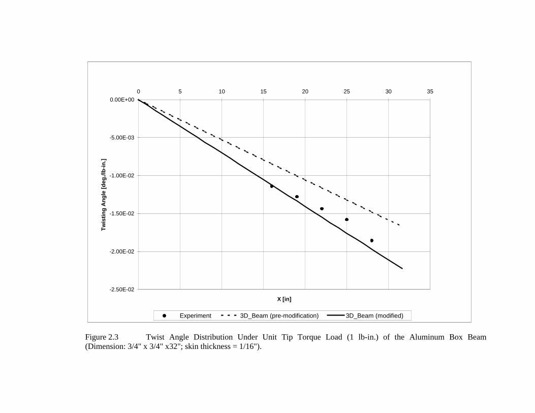
The external dimensions of the aluminum box beam are 3/4" (width), 3/4" (depth)and 32" (long). The skin thickness is 1/16". The aluminum box beam was subjected toboth bending and torsion tests. The normalized test and numerical results are shown inFigure 2.2 and 2.3. Before the modifications, the predicted results underestimated theexperimental values. The modifications based on Plane Stress assumption improve theprediction. It should be noted that the effect of torsion-related out-of-plane warping is notseen in Figure 2.3 as there is no warping for a square aluminum box with constant skinthickness.

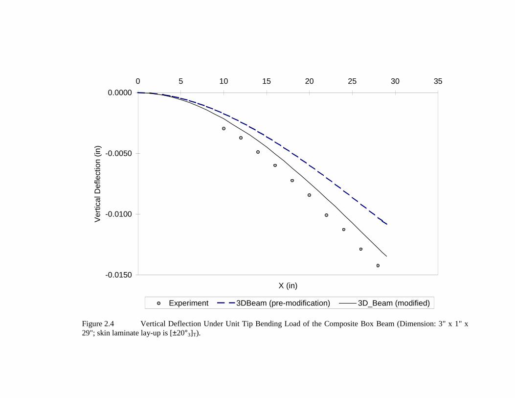
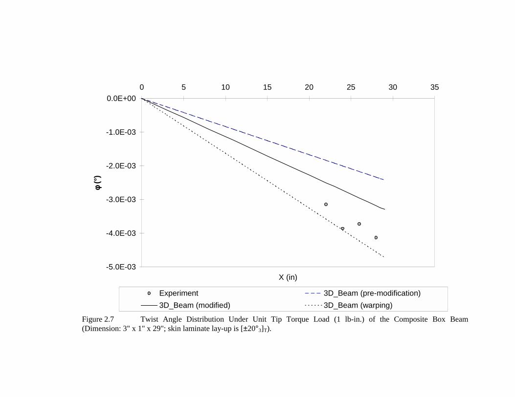
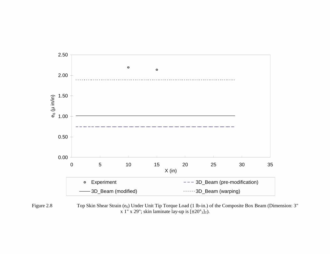
2.2.2 Composite Box Beam

The external dimensions of the composite box beam are 3" (width), 1" (depth) and29" (length). The lay-up of the composite skin is [±20°3]T. The ply material of thelaminate skin is LTM-45, and the properties of the ply are given in Table 2.1.

The composite box beam was subjected to both the bending and torsion tests. Themeasured parameters were the vertical deflection, the twisting angle and strains at twolongitudinal locations (x=10" and 15" from the built-in end).

Comparisons between the experimental results and numerical results for thebending test are shown in Figures 2.4 - 2.6. The 3D-Beam's prediction improves after themodifications. It is also noted that the transverse strain (e2) is not negligible and, in fact,has the same order of magnitude as longitudinal strain (e1). The data shows that ourformulation based on the assumption that the transverse stress (σ2) equals zero is moreeffective than that of zero transverse strain (e2).

The comparisons between the experimental results and numerical results for thetorsion test are shown in Figures 2.7 and 2.8. The comparsion indicates the 3D-Beampredictions (modified with warping effect) are close to the experimental results. It is alsonoted that the shear strain (e6) is nearly double if the warping effect is included.

6

Description LTM-45

(Graphite/Epoxy)

Ex(msi) 18.3

Ey(msi) 1.3

Es(msi) 0.9

νx 0.28

Table 2.1 Ply Properties of LTM-45. Ex is the elastic modulus of the ply inthe x (longitudinal axis of the fiber) direction. Ey is the elastic modulus of theply in the y (transverse) direction. And Es refers to the shear modulus of theply.

X1

X2

X3

θ

1

2

3

σ4σ5

σ3

σ6σ1

σ5

σ2

σ6

σ4

Figure 2.1 Definition of Coordinate System & Notations (X1 is along the beam axis)

-0.1

-0.08

-0.06

-0.04

-0.02

00 5 10 15 20 25 30 35

X (in)

Vert

ical

Def

lect

ion

(in/lb

)

Experiment 3D_Beam (pre-modification) 3D-Beam (modified)

Figure 2.2 Vertical Deflection Under Unit Tip Bending Load of the Aluminum Box Beam (Dimension: 3/4" x 3/4"x32"; skin thickness = 1/16").

-2.50E-02

-2.00E-02

-1.50E-02

-1.00E-02

-5.00E-03

0.00E+000 5 10 15 20 25 30 35

X [in]

Twis

ting

Ang

le [d

eg./l

b-in

.]

Experiment 3D_Beam (pre-modification) 3D_Beam (modified)

Figure 2.3 Twist Angle Distribution Under Unit Tip Torque Load (1 lb-in.) of the Aluminum Box Beam(Dimension: 3/4" x 3/4" x32"; skin thickness = 1/16").

-0.0150

-0.0100

-0.0050

0.00000 5 10 15 20 25 30 35

X (in)

Verti

cal D

efle

ctio

n (in

)

Experiment 3DBeam (pre-modification) 3D_Beam (modified)

Figure 2.4 Vertical Deflection Under Unit Tip Bending Load of the Composite Box Beam (Dimension: 3" x 1" x29"; skin laminate lay-up is [±20°3]T).

0

5

10

15

20

250 5 10 15 20 25 30 35

X (in)

e 1 (µ

in/in

)

Experiment 3D_Beam (pre-modification) 3D_Beam (modified)

Figure 2.5 Top Skin Longitudinal Strain (e1) Under Unit Tip Bending Load of the Composite Box Beam(Dimension: 3" x 1" x 29"; skin laminate lay-up is [±20°3]T).

-40

-30

-20

-10

0

100 5 10 15 20 25 30 35

X (in)

e 2 ( µ

in/in

)

Experiment 3D_Beam (pre-modification) 3D_Beam (modified)

Figure 2.6 Top Skin Transverse Strain (e2) Under Unit Tip Bending Load of the Composite Box Beam (Dimension:3" x 1" x 29"; skin laminate lay-up is [±20°3]T).

-5.0E-03

-4.0E-03

-3.0E-03

-2.0E-03

-1.0E-03

0.0E+000 5 10 15 20 25 30 35

X (in)

φφ φφ (°

)

Experiment 3D_Beam (pre-modification) 3D_Beam (modified) 3D_Beam (warping)

Figure 2.7 Twist Angle Distribution Under Unit Tip Torque Load (1 lb-in.) of the Composite Box Beam(Dimension: 3" x 1" x 29"; skin laminate lay-up is [±20°3]T).

0.00

0.50

1.00

1.50

2.00

2.50

0 5 10 15 20 25 30 35X (in)

e 6 (µ

in/in

)

Experiment 3D_Beam (pre-modification)

3D_Beam (modified) 3D_Beam (warping)

Figure 2.8 Top Skin Shear Strain (e6) Under Unit Tip Torque Load (1 lb-in.) of the Composite Box Beam (Dimension: 3"x 1" x 29"; skin laminate lay-up is [±20°3]T).

Chapter 3

Parametric Study

Before we start to design a D-spar that meets specific structural properties and hasmaximum bend-induced twist, we would like to understand how various designparameters influence the bend-twist coupling coefficient. We first derive a simpleexpression of the coupling coefficient for a flat-plate laminate. We then use 3D-Beamsoftware to carry out the parametric study for the D-spar.

3.1 Theoretical Estimation of the Coupling Coefficient, α

Instead of immediately performing a numerical estimation of the α interaction

parameter for the D-spar, we explored the possibility of estimating the maximum value ofthe α interaction parameter theoretically to gain some physical insight into bend-twistand extension-twist coupling.

We assume the problem we are looking at is a two-dimensional flat laminate andthe in-plane normal stress in the ‘2’ direction has the value of zero; i.e., σ2 = 0.

The constituent relationship between stress and strain is

=

6

2

666261

262221

161211

6

2

1 1

εεε

σσσ

QQQQQQQQQ

(3.1)

If σ2 = 0, we can reduce the Qs matrix as follows,

=

6

1

6661

1611

6

1

εε

σσ

QQQQ

where

22

21121111

*Q

QQQQ −=

22

26121616

*Q

QQQQ −=

22

21626161

*Q

QQQQ −=

22

26626666

*Q

QQQQ −= (3.2)

The relationship between the in-plane strains ( 01ε , 0

6ε ), ( 1κ , 6κ ) and N1, N6, M1,M6 is as follows

=

6

1

06

01

66616616

16116111

66616661

16111611

6

1

6

1

κκεε

DDBBDDBBBBAABBAA

MMNN

(3.3)

where

∫= dzQA ijij

∫= dzzQB ijij *

∫= dzzQD ijij2*

curvaturestwistingandbendingstrainsshearandnormalplanein

::,

6,1

06

01

κκεε −

N1, N6 : in-plane normal force and shear force per unit width

M1, M6 : bending moment and twisting moment per unit width

z : the vertical distance between the mid-plane and the ply layer

For a symmetric (symmetry with respect to the mid-plane) laminate, the relationreduces to

=

6

1

06

01

6661

1611

6661

1611

6

1

6

1

0000

0000

κκεε

DDDD

AAAA

MMNN

(3.4)

For a symmetric laminate, there are two types of coupling:

a. Extension – Shear coupling

b. Bend – Twist coupling.

For an anti-symmetric laminate, the relation reduces to

=

6

1

06

01

6616

1161

6166

1611

6

1

6

1

000000

00

κκεε

DBDBBA

BA

MMNN

(3.5)

In this case, the coupling is different from the previous case. The couplings are

a. Extension – Twist coupling

b. Bend – Shear coupling.

If a laminate is not symmetric or anti-symmetric, there will be more than twomodes of coupling. The stiffness and compliance matrix will be fully populated.

How do the ijijij DBA ,, values relate to the “EI”, “GJ” and “g” of Lobitz’swork? Let us reprint some of the equations in Lobitz’s work9 that are applicable to ourderivation. The equations that Lobitz used for the extension-twist coupling are given inmatrix form below:

=

∂∂∂∂

−

−

tMF

x

xu

GJggEA

ϕ (Eq. 1 in Lobitz and Veers9)

=

∂∂∂∂

−

−

t

bMM

x

xGJg

gEIϕ

θ

(Eq. 6 in Lobitz and Veers9)

The terms are defined in Lobitz.9 For the strain terms, the terms xu

∂∂ ,

x∂∂ϕ and

x∂∂θ

equal to 01ε , 6κ and 1κ respectively. For the force terms, the F, Mt and Mb equal to b*N1

b*M6 and b*M1 respectively. The parameter “b” is the width of the flat laminate.

The “EI”, “GJ”, “g” can be expressed by Aij, Bij and Dij as follows:

Bend-Twist Coupling (Symmetry)

6611

16

16

66

11

** DDD

GJEIg

bgD

bGJD

bEID

−==

−=

=

=

α

If a laminate has a lay-up of [θ]S (single orientation), the α is further reduced to

)*(*)*(

**

* 2262266

2122211

26122216

6611

16

QQQQQQ

QQQQ

QQ

Q

−−

−−=−=α (3.6)

Extension-Twist Coupling (Antisymmetry)

6611

16

16

66

11

** DA

BGJEA

g

bgB

bGJD

bEAA

−==

−=

=

=

α

If a laminate has a lay-up of [θ]AS (single orientation), the α is further reduced to

)*(*)*(

***43

**

43

2262266

2122211

26122216

6611

16

QQQQQQ

QQQQ

QQ

Q

−−

−−=

−=α

(3.7)

The α interaction parameters are related to the normal coupling coefficient (ν16) and theshear coupling coefficient (ν61). The two coefficients are defined as follows12:

2122211

1622261216

***

QQQQQQQ

−−=ν

2266622

1622261261

***

QQQQQQQ

−−=ν (3.8)

Therefore, the α interaction parameters are reduced to the simplest form:

Bend-Twist Coupling

61162 *ννα = (3.9)

Extension-Twist Coupling

61162 **

43 ννα = (3.10)

It is interesting to note that after all the algebraic manipulations, we have obtaineda simple form for the α interaction parameter for a flat-plate laminate. This leads to somephysical insights: first, the interaction parameter, α, is highly dependent on the plymaterial, since both the ν16 and ν61 coefficients are material-dependent; second, thegeometry parameters do not appear in the simplified equation. This implies that thegeometrical parameters may not affect the determination of the range of the α. However,for the second observation, we are dealing with a simple type of laminate; that is a flatsurface, symmetric or anti-symmetric laminate.

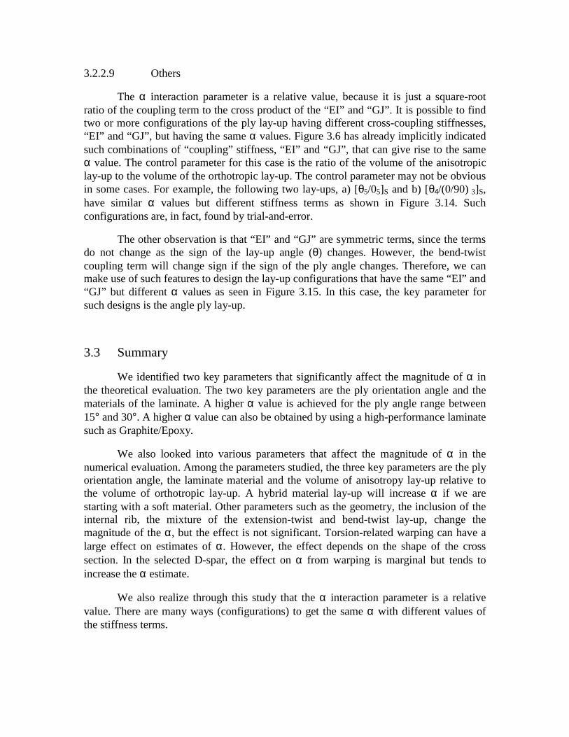
Two typical ply materials, a) T800/3900-2 (Graphite/Epoxy) and b) Scotchply(Glass/Epoxy) are being studied. The ply properties of these materials are given in Table3.1. The α interaction parameters for a flat plate laminate made out of these two types ofmaterials are shown in Figure 3.1.

It is clearly seen that the range of α interaction parameters depends very much onthe type of material chosen. Graphite/Epoxy has a maximum value close to 0.8, andGlass/Epoxy has a maximum value close to 0.5. The maximum values of α for thesematerials occur at different ply orientations. In general, we can state that the highervalues of α occur in ply orientation, θ , between 15° and 30°. In subsequent sections, welook into other parameters that affect the α interaction parameters numerically.

3.2 Numerical Estimation of the Coupling Coefficient, α

3.2.1 D-spar Geometry

In the numerical study, we study a D-spar composite structure, which is part ofthe airfoil shape. The basic dimension of the D-spar is 72" (long), 6" (wide) and 3"(height) as shown in Figure 3.2. The radius of the semi-circle is 1.5”. Effectively, thewidth of the horizontal surface is 4.5".

The lay-up sequence at the top and bottom surface affects the lay-up sequence atthe left vertical and right semi-circular walls. If the top and bottom laminates are

symmetric lay-ups, then the lay-up at the two walls will be anti-symmetric. On the otherhand, if the top and bottom laminates are anti-symmetric lay-ups, then the lay-up at thetwo walls will be symmetric.

We also need to standardize the lay-up notation. The notation [θn]s refers to ‘n’layers of θ ply, and the subscript ‘s’ denotes that the lay-up is symmetric in reference tothe mid-plane between top and bottom surfaces. The notation [θn]AS refers to ‘n’ layers ofθ ply, and the subscript ‘AS’ denotes that the lay-up is anti-symmetric in reference to themid-plane between top and bottom surfaces.

3.2.2 Parametric Study

In this parametric study we investigate various parameters that affect the range ofα interaction parameters (mainly for Bend-Twist coupling). The parameters that we haveconsidered are:

a. geometry,

b. ply materials (Graphite/Epoxy and Glass/Epoxy),

c. laminate thickness,

d. volumetric fraction of the anisotropy,

e. internal spar or rib,

f. hybrid materials,

g. mixtures of extension-twist and bend-twist lay up,

h. torsion-related out-of-plane warping, and

i. others such as

(i) configurations that exhibit the same “α” but have different “EI”and “GJ”

(ii) configurations that exhibit different “α” but have the same “EI”and “GJ”

3.2.2.1 Geometry Effect

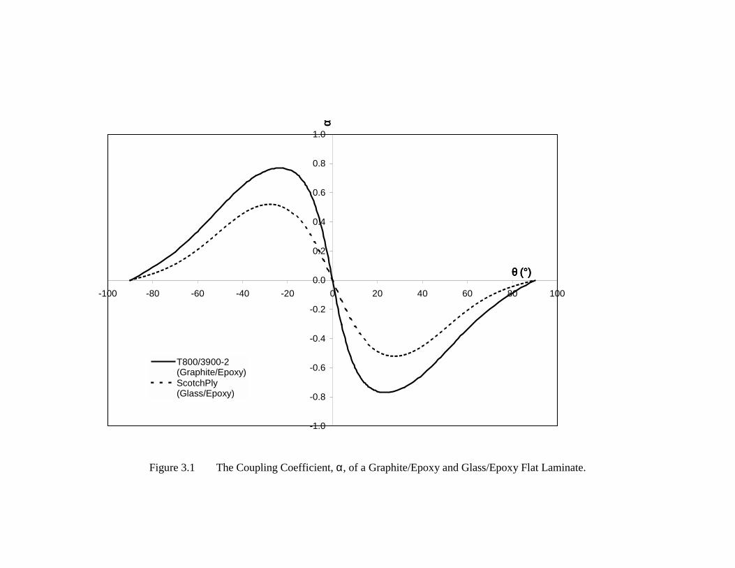
We looked into two different cross-sectional dimensions of the D-spar: a) 6” x 3”and b) 6” x 4”. The results are shown in Figures 3.3a-c. The α interaction parameter doeschange as we change the height of the D-spar. However, the variation is negligible.

A relevant case for wind turbine blades is to compare the D-spar with an airfoilshape. We compute the α interaction parameter for a 3-inch thick NACA0012 airfoil (25”chord) and compare the results against the 6” x 3” D-spar. We observe that there are

negligible effects from the geometry factor in the case of the thin-wall assumption as seenin Figure 3.3b.

We assume that the transverse shear through the thickness is negligible in thethin-wall case. On the other hand, the transverse shear effect is included in the thick-wallformulation. This leads to increasing the torsion rigidity of the D-spar and results in asmaller α as seen in Figure 3.3d. Since the wall thickness (0.2” to 0.3”) of the D-spar issmall as compared with the height (3” to 4”) of the D-spar, the thin-wall formulation ismore appropriate .

3.2.2.2 Material Effect

From the theoretical estimation of the α interaction parameter, we find that the αis highly dependent on the types of material used. For the D-spar, we also expect to see asignificant effect of the material as we look at both the Graphite/Epoxy and Glass/Epoxy.The numerical results are shown in Figures 3.4a-c. The maximum α achievable for thegraphite and glass materials is 0.62 and 0.42 respectively. The results indicate that theratio of the maximum α for the two materials is about 3/2 (Graphite/Glass).

3.2.2.3 Thickness Effect

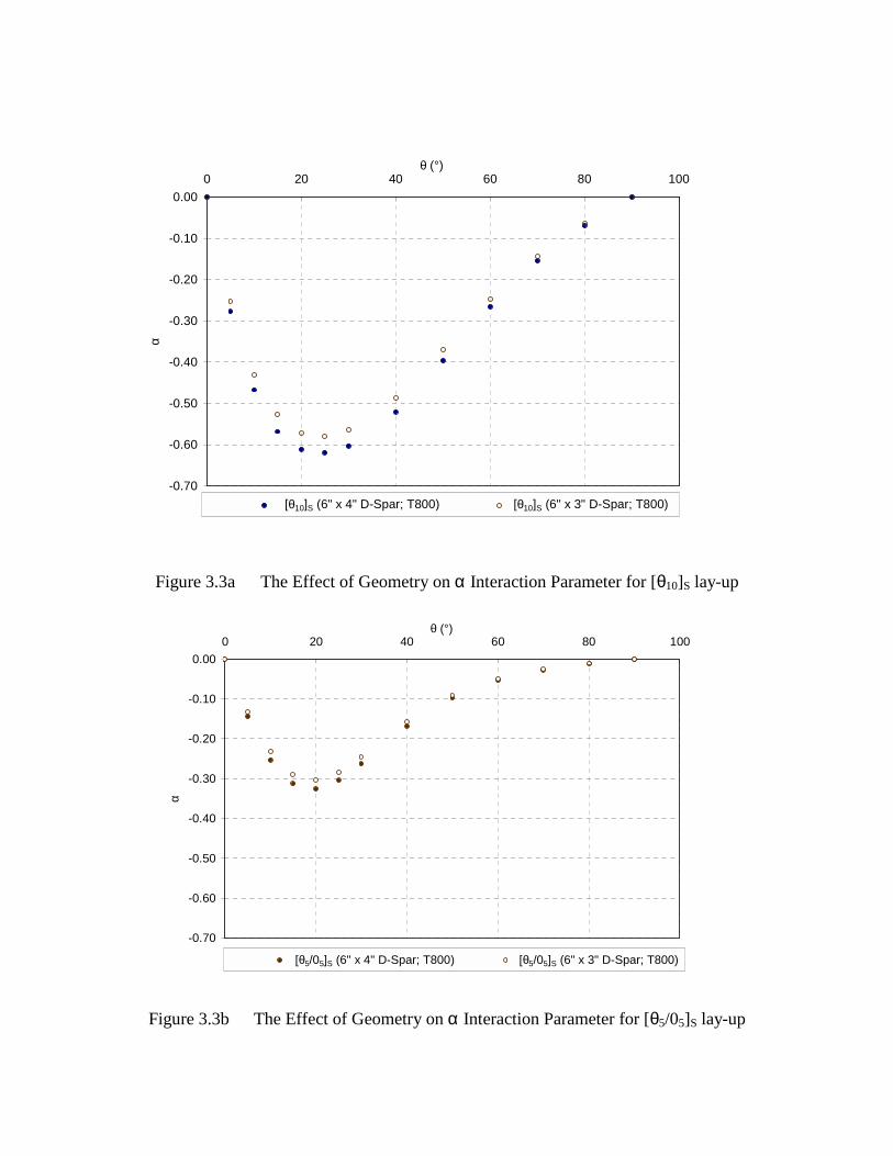
We have two approaches to studying the effects of the laminate thickness. Thefirst approach is to fix the ply distribution, but to increase or decrease the total laminatethickness. For example, if we have a [θn/φm]S laminate, the distribution ratio is n/m(orm/n). If we assume each ply has the same thickness (t), then the total thickness is(m+n)*t. We proceed with changing the total thickness by varying the “m”, “n” layers ofplies but keeping the distribution ratio (n/m or m/n) constant. With this arrangement, wesee that the α interaction parameter remains constant as shown in Figure 3.5a.

The second approach is to keep the total laminate thickness constant and vary thedistribution ratio. We looked into various configurations. We observed that the αinteraction parameter varies with the distribution ratio as in Figure 3.5b.

3.2.2.4 Anisotropy Volumetric Effect

Figure 3.5 indicates that the volumetric distribution of the ply within the laminatehas a dominant effect on the α interaction parameter. To further study this effect welooked into a laminate that has ply orientation, [20n/[45/-45]m]S, where m=2, 3, 4. Wethen varied the parameter ‘n’ to simulate change in the total thickness as well as thedistribution ratio (the volume fraction Va of anisotropic fibers is then n/(2*m+n)). Theresults are shown in Figure 3.6. The upper portion of the figure shows that for the samenumber of 20° plies but different values of Va, we have different values of α. However, ifwe adjust the number of layers of 20° plies (n) in such a way that the three configurationshave the same value of Va, we will get a single value of α as seen in the lower portion ofFigure 3.6.

Therefore, for a laminate with a fixed set of ply orientations, the α interactionparameter for that laminate is determined by the volume fraction of the anisotropic pliesregardless of distribution ratio.

3.2.2.5 Internal Spar Effects

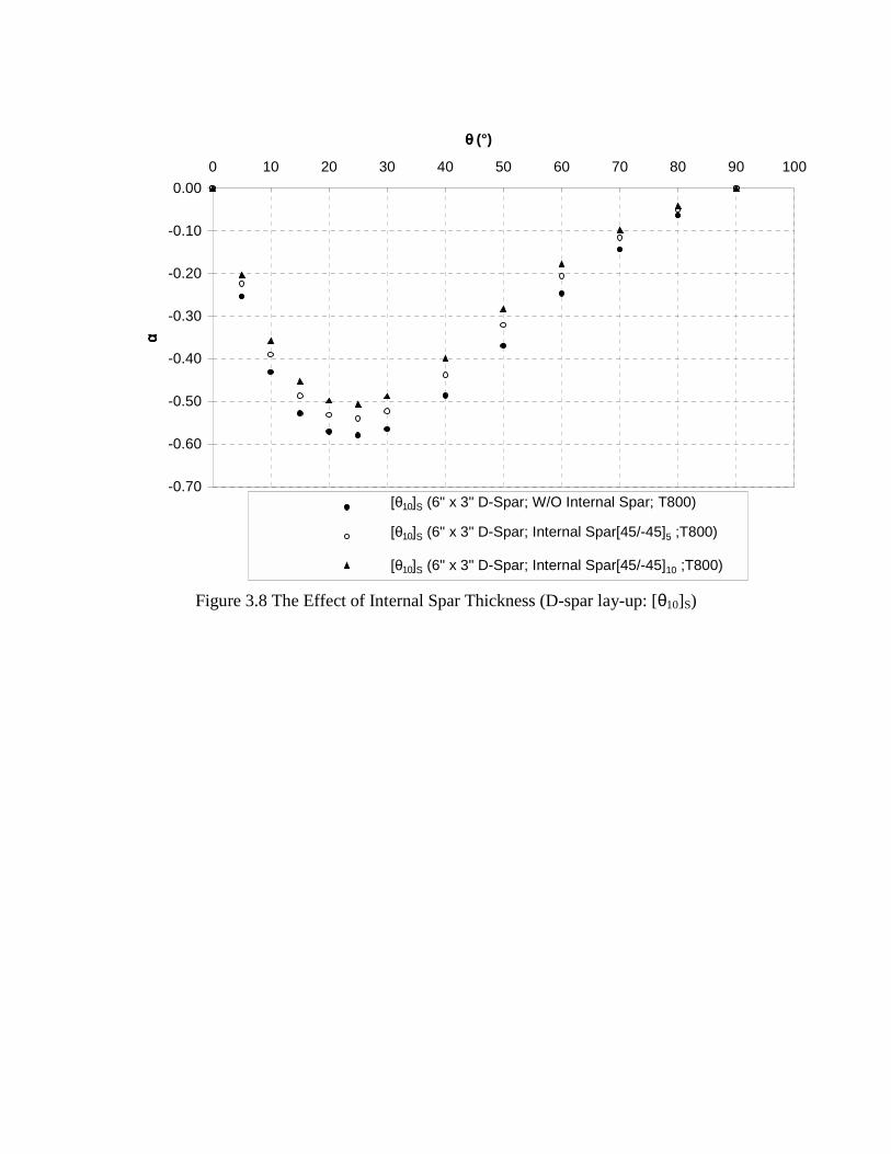
An internal spar is inserted at the end-edge of the semi-circle as shown in Figure3.7. The insertion of an internal spar increases the “EI” and “GJ”, and will result in areduction of the α interaction parameter. We look into both the effects of the thicknessand ply orientation of the internal spar. If we increase the thickness of the internal sparwhile having the same ply orientation, the α interaction parameter reduces, as shown inFigure 3.8.

The next case considered the constant thickness of the internal spar while varyingthe ply orientation of the internal spar. The result is shown in Figure 3.9a. The resultindicates that the ply orientation of the D-spar has small effect on the α interactionparameter. The variation of the α interaction parameter with and without an internal sparis about 10%.

In fact, the internal spar has changed significantly the stiffness properties of theD-spar in the lead-lag direction. Figure 3.9b shows the Dij of the D-spar with and withoutan internal spar (same thickness but different orientation). We can see that the D22 (lead-lag) changes substantially.

3.2.2.6 Hybrid Materials Effect

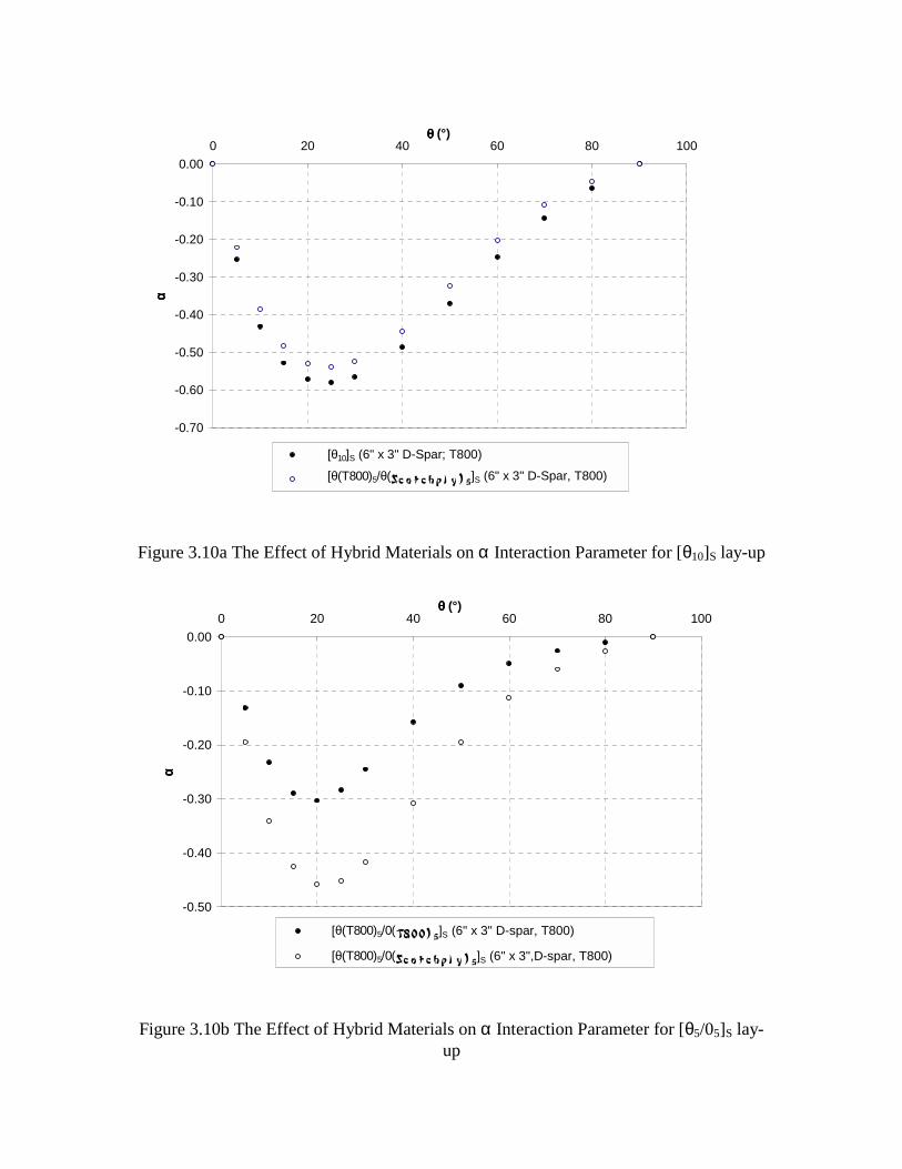
To study this effect, we looked at three baseline configurations and comparedtheir results against the same configurations with hybrid material (for all the cases wesubstituted graphite/epoxy for glass/epoxy). The three configurations we studied are[θ(T800)5/θ(Scotchply)5]S, [θ(T800)5/0(Scotchply)5]S, [θ(T800)5/90(Scotchply)5]S andthe results are shown in Figures 3.10a-c.

In the first case, we have 50% graphite fibers and 50% glass fibers all at the sameply orientation. The α interaction parameter of this hybrid case should be lower than theall-graphite case and higher than the all-glass case (see Figure 3.10a). Therefore, thereduction or increase of α depends on the baseline configurations. The lower bound ofthe α interaction parameter is limited by the low-performance fibers (glass) and the upperbound is limited by the high-performance fibers (graphite).

In the second case (see Figure 3.10b), the change is at the 0° material. Wereplaced 0° graphite fibers with 0° glass fibers or vice versa. The substantial change in αcomes mainly from a large change in “EI” because the ratio of the Ex (graphite/fiber) isabout 4 to 1. We can deduce that if the volume fraction of non-anisotropic fibers is oflower stiffness than the anisotropic ones, then we can achieve a higher α value.

In the third case (see Figure 3.10c), the change is at the 90° material. We replaced90° graphite fibers with 90° glass fibers or vice versa. The change in α is marginal

because there is marginal change in the Ey (transverse ply stiffness) and the Es (shearmodulus) for both materials.

In fact, the dominant effect of using hybrid materials is the significant change inflapping stiffness as shown in Figure 3.11. Note that the change of D12 between the solidand hollow cross sections cannot be seen in Figure 3.11 because the change is small

3.2.2.7 The Effect of Mixtures of Antisymmetry and Symmetry Lay-Up

Until now we have been looking at a D-spar with symmetric lay-up, and thebehavior of the D-spar is quite clear (bend-twist or tension-shear mode). If we replacesome of the symmetric lay-up with an anti-symmetric lay-up, the behavior of the D-sparwill be very complicated. The following matrices show the change in stiffness matrixfrom the symmetric ply lay-up to the mixture of symmetric and antisymmetric ply lay-up.

]&[

00

00

0000

0000

666116

161161

616661

161611

6661

1611

6661

1611

ryantisymmetsymmetrymixtureSymmetry

DDBDDB

BAABAA

DDDD

AAAA

→

→

Instead of just bend-twist coupling for the symmetric lay-up, we have complexcoupling among bend, twist and shear modes. In fact, the compliance matrix of thismixture is fully populated, therefore it is difficult to control the desired mode of coupling.In addition to that, the α interaction parameter reduces as we increase the degree ofmixture as shown in Figure 3.12. The insertion of core is just to clarify the notation, andit does not affect the calculation. The term “core” signifies that the D-spar is hollow.

3.2.2.8 Torsion-Related Out-of-Plane Warping

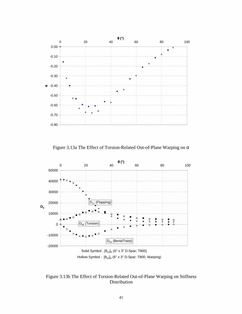
The effect of warping on the α interaction parameter is hard to evaluate. Thereason is that it is difficult to include a warping function applicable to all cases in the 3D-Beam software. The warping function depends greatly on the geometry of the cross-sectional shape. We assume the shape of the D-spar is “similar” to the shape of arectangular section, therefore, a simple bi-linear warping function was implemented inthe 3D-Beam.

The torsion-related warping, as seen in Figures 3.13a-b, generally increases the αinteraction parameter. The changes in the α values come from the reduction in “GJ” andincrease in the “coupling” stiffness, while the “EI” remains unchanged. For other cross-section shapes, we expect the α will change if the torsion-related warping is included.

3.2.2.9 Others

The α interaction parameter is a relative value, because it is just a square-rootratio of the coupling term to the cross product of the “EI” and “GJ”. It is possible to findtwo or more configurations of the ply lay-up having different cross-coupling stiffnesses,“EI” and “GJ”, but having the same α values. Figure 3.6 has already implicitly indicatedsuch combinations of “coupling” stiffness, “EI” and “GJ”, that can give rise to the sameα value. The control parameter for this case is the ratio of the volume of the anisotropiclay-up to the volume of the orthotropic lay-up. The control parameter may not be obviousin some cases. For example, the following two lay-ups, a) [θ5/05]S and b) [θ4/(0/90) 3]S,have similar α values but different stiffness terms as shown in Figure 3.14. Suchconfigurations are, in fact, found by trial-and-error.

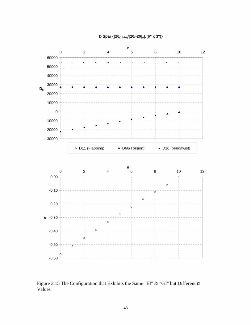
The other observation is that “EI” and “GJ” are symmetric terms, since the termsdo not change as the sign of the lay-up angle (θ) changes. However, the bend-twistcoupling term will change sign if the sign of the ply angle changes. Therefore, we canmake use of such features to design the lay-up configurations that have the same “EI” and“GJ” but different α values as seen in Figure 3.15. In this case, the key parameter forsuch designs is the angle ply lay-up.

3.3 Summary

We identified two key parameters that significantly affect the magnitude of α inthe theoretical evaluation. The two key parameters are the ply orientation angle and thematerials of the laminate. A higher α value is achieved for the ply angle range between15° and 30°. A higher α value can also be obtained by using a high-performance laminatesuch as Graphite/Epoxy.

We also looked into various parameters that affect the magnitude of α in thenumerical evaluation. Among the parameters studied, the three key parameters are the plyorientation angle, the laminate material and the volume of anisotropy lay-up relative tothe volume of orthotropic lay-up. A hybrid material lay-up will increase α if we arestarting with a soft material. Other parameters such as the geometry, the inclusion of theinternal rib, the mixture of the extension-twist and bend-twist lay-up, change themagnitude of the α, but the effect is not significant. Torsion-related warping can have alarge effect on estimates of α. However, the effect depends on the shape of the crosssection. In the selected D-spar, the effect on α from warping is marginal but tends toincrease the α estimate.

We also realize through this study that the α interaction parameter is a relativevalue. There are many ways (configurations) to get the same α with different values ofthe stiffness terms.

Description T800/3900-2

(Graphite/Epoxy)

Scotchply

(Glass/Epoxy)

Ex(msi) 23.2 5.6

Ey(msi) 1.0 1.2

Es(msi) 0.9 0.66

νx 0.28 0.3

Table 3.1 Ply Properties of T800/3900-2 and Scotchply. Ex is the elastic modulus of theply in the x (longitudinal axis of the fiber) direction. Ey is the elastic modulus of the plyin the y (transverse) direction. And Es refers to the shear modulus of the ply.

-1.0

-0.8

-0.6

-0.4

-0.2

0.0

0.2

0.4

0.6

0.8

1.0

-100 -80 -60 -40 -20 0 20 40 60 80 100

θ (°)θ (°)θ (°)θ (°)

αα αα

T800/3900-2(Graphite/Epoxy)ScotchPly(Glass/Epoxy)

Figure 3.1 The Coupling Coefficient, α, of a Graphite/Epoxy and Glass/Epoxy Flat Laminate.

radius=1.5"

4.5"

6"

3"

Figure 3.2 D-spar Cross-Section Shape

4.5"

6"

3"

Inte

rnal

Spa

r

Figure 3.7 D-spar with Internal Spar

-0.70

-0.60

-0.50

-0.40

-0.30

-0.20

-0.10

0.000 20 40 60 80 100

θ (°)α

[θ10]S (6" x 3" D-Spar; T800)[θ10]S (6" x 4" D-Spar; T800)

Figure 3.3a The Effect of Geometry on α Interaction Parameter for [θ10]S lay-up

-0.70

-0.60

-0.50

-0.40

-0.30

-0.20

-0.10

0.000 20 40 60 80 100

θ (°)

α

[θ5/05]S (6" x 3" D-Spar; T800)[θ5/05]S (6" x 4" D-Spar; T800)

Figure 3.3b The Effect of Geometry on α Interaction Parameter for [θ5/05]S lay-up

-0.70

-0.60

-0.50

-0.40

-0.30

-0.20

-0.10

0.000 20 40 60 80 100

θ (°)α

[θ5/905]S (6" x 3" D-Spar; T800)[θ5/905]S (6" x 4" D-Spar; T800)

Figure 3.3c The Effect of Geometry on α Interaction Parameter for [θ5/905]S lay-up

-0.70

-0.60

-0.50

-0.40

-0.30

-0.20

-0.10

0.000 10 20 30 40 50 60 70 80 90 100

θ θ θ θ (°)

α α α α

[θ10]S (6" x 3" D-Spar; Thick Wall)

[θ10]S (NACA0012; 25" Chord; Thick Wall) [θ10]S (NACA0012; 25" Chord; Thin Wall)

[θ10]S (6" x 3" D-Spar; Thin Wall)

Figure 3.3d The Effects of Thick/Thin Wall Assumption on α Interaction Parameter

-0.7

-0.6

-0.5

-0.4

-0.3

-0.2

-0.1

00 10 20 30 40 50 60 70 80 90

θθθθ (°)

α α α α

[θ10]S (6" x 4" D-Spar;Scotchply)[θ10]S (6" x 4" D-Spar;T800)

Figure 3.4a The Effects of Materials on α Interaction Parameter for [θ10]S lay-up

-0.7

-0.6

-0.5

-0.4

-0.3

-0.2

-0.1

00 10 20 30 40 50 60 70 80 90

θθθθ (°)

α α α α

[θ5/05]S (6" x 4" D-Spar; T800) [θ5/05]S (6" x 4" D-Spar; Scotchply)

Figure 3.4b The Effects of Materials on α Interaction Parameter for [θ5/05]S lay-up

-0.7

-0.6

-0.5

-0.4

-0.3

-0.2

-0.1

00 20 40 60 80 100

θθθθ (°)α α α α

[θ5/905]S (6" x 4" D-Spar; Scotchply)[θ5/905]S (6" x 4" D-Spar; T800)

Figure 3.4c The Effects of Materials on α Interaction Parameter for [θ5/905]S lay-up

-0.7

-0.6

-0.5

-0.4

-0.3

-0.2

-0.1

00 5 10 15 20 25 30 35 40

Total # of Layers (n)α α α α

[200.6n/600.4n]S[20n]S [200.6n/[60/−6060/−6060/−6060/−60]0.2n]S

Figure 3.5a The Effects of Ply Thickness for a given distribution for 6" x 4" D-spar

-0.7

-0.6

-0.5

-0.4

-0.3

-0.2

-0.1

00 2 4 6 8 10 12

n

α α α α

[20n/0(10-n)]S [20n/90(10-n)]S[20n/45(10-n)]S [20n/60(10-n)]S[20n/30(10-n)]S

Figure 3.5b The Effects of Ply Thickness & Distribution for 6" x 4" D-spar

-0.7

-0.6

-0.5

-0.4

-0.3

-0.2

-0.1

00 5 10 15 20 25 30 35 40 45 50

n Layers of 20° ply α α α α

[20n/[45/−4545/−4545/−4545/−45]3]S[20n/[45/−4545/−4545/−4545/−45]4]S [20n/[45/−4545/−4545/−4545/−45]2]S

Va

-0.7

-0.6

-0.5

-0.4

-0.3

-0.2

-0.1

00 0.1 0.2 0.3 0.4 0.5 0.6 0.7 0.8 0.9 1

α

[20n/[45/−4545/−4545/−4545/−45]3]S[20n/[45/−4545/−4545/−4545/−45]4]S [20n/[45/−4545/−4545/−4545/−45]2]S

Figure 3.6 The Effect of Anisotropic Volumetric Ratio on α for 6" x 4" D-Spar

-0.70

-0.60

-0.50

-0.40

-0.30

-0.20

-0.10

0.000 10 20 30 40 50 60 70 80 90 100

θ θ θ θ (°)α α α α

[θ10]S (6" x 3" D-Spar; W/O Internal Spar; T800)

[θ10]S (6" x 3" D-Spar; Internal Spar[45/-45]5 ;T800)

[θ10]S (6" x 3" D-Spar; Internal Spar[45/-45]10 ;T800)

Figure 3.8 The Effect of Internal Spar Thickness (D-spar lay-up: [θ10]S)

-0.60

-0.50

-0.40

-0.30

-0.20

-0.10

0.00[No RIB] [0]_20 [30]_20 [45]_20 [60]_20 [90]_20 [30/-30]_10 [45/-45]_10 [60/-60]_10

Internal Spar Lay Up [θθθθ]20 or [θ/−θθ/−θθ/−θθ/−θ]10αα αα

Figure 3.9a The Effect of Internal Spar Ply Orientation (D-spar lay-up: [2010]S)

-2.E+04

0.E+00

2.E+04

4.E+04

6.E+04

8.E+04

1.E+05

1.E+05

1.E+05

[No RIB] [0]_20 [30]_20 [45]_20 [60]_20 [90]_20 [30/-30]_10 [45/-45]_10 [60/-60]_10

Internal Spar Lay Up [θθθθ]20 or [θ/−θθ/−θθ/−θθ/−θ]10

Dij

D66(Torsion) D11(Flapping) D22(Lead-Lag) D16(Flap/Twist)

Figure 3.9b The Effect of Internal Spar Ply Orientation (D-spar lay-up: [2010]S)

-0.70

-0.60

-0.50

-0.40

-0.30

-0.20

-0.10

0.000 20 40 60 80 100

θθθθ (°)

α α α α

[θ10]S (6" x 3" D-Spar; T800)[θ(Τ800)5/θ(Sc o t c h p l y ) 5]S (6" x 3" D-Spar, T800)

Figure 3.10a The Effect of Hybrid Materials on α Interaction Parameter for [θ10]S lay-up

-0.50

-0.40

-0.30

-0.20

-0.10

0.000 20 40 60 80 100

θθθθ (°)

α α α α

[θ(Τ800)5/0(T800) 5]S (6" x 3" D-spar, T800)

[θ(Τ800)5/0(Sc o t c hp l y ) 5]S (6" x 3",D-spar, T800)

Figure 3.10b The Effect of Hybrid Materials on α Interaction Parameter for [θ5/05]S lay-up

-0.60

-0.50

-0.40

-0.30

-0.20

-0.10

0.000 20 40 60 80 100

θθθθ (°)

α α α α

[θ(Τ800)5/90(T800) 5]S (6" x 3" D-spar, T800)

[θ(Τ800)5/90(Sc o t c hp l y ) 5]S (6" x 3" D-spar,T800)

Figure 3.10c The Effect of Hybrid Materials on α Interaction Parameter for [θ5/905]S lay-up

-10000

0

10000

20000

30000

40000

500000 20 40 60 80 100

θθθθ (°)

Dij

D66 (Torsion) D11 (Flapping) D12(Bending_twist)D66 (Torsion) D11 (Flapping) D12(Bending_twist)

Solid : [θ5/05]S (6" x 3" ; T800)

Hollow: [θ(Τ800)5/0(Scotchply) 5]S (6" x 3")

Figure 3.11 The Effect of Hybrid Materials on Dij

-0.70

-0.60

-0.50

-0.40

-0.30

-0.20

-0.10

0.000 20 40 60 80 100

θθθθ (°)α α α α

[θ10/CORE/θ10]

[θ8/θ2/CORE/−θ2/θ8]

[θ6/θ4/CORE/−θ4/θ6]

[θ4/θ6/CORE/−θ6/θ4]

[θ2/θ8/CORE/−θ8/θ2]

"CORE" is hollow.

Figure 3.12 The Effect of Antisymmetry on α Interaction Parameter

41

-0.80

-0.70

-0.60

-0.50

-0.40

-0.30

-0.20

-0.10

0.000 20 40 60 80 100

θθθθ (°)

α α α α

Figure 3.13a The Effect of Torsion-Related Out-of-Plane Warping on α

-20000

-10000

0

10000

20000

30000

40000

500000 20 40 60 80 100

θθθθ (°)

Solid Symbol : [θ10]S (6" x 3" D-Spar; T800)

Hollow Symbol : [θ10]S (6" x 3" D-Spar; T800; Warping)

D11 (Flapping)

D66 (Torsion)

D16 (Bend/Twist)

Dij

Figure 3.13b The Effect of Torsion-Related Out-of-Plane Warping on StiffnessDistribution

42

-0.35

-0.30

-0.25

-0.20

-0.15

-0.10

-0.05

0.000 20 40 60 80 100

θθθθ (°)α α α α

[θ5/05]S (6" x 3" D-Spar; T800) [θ4/[0/90]3]S (6" x 3" D-Spar; T800)

-10000

0

10000

20000

30000

40000

500000 10 20 30 40 50 60 70 80 90

θθθθ (°)

Solid Symbol : [θ5/05]S (6" x 3" D-Spar; T800)

Hollow Symbol : [θ4/[0/90]3]S (6" x 3" D-Spar; T800)

D11 (Flapping)

D66 (Torsion)

D16 (Bend/Twist)

Dij

Figure 3.14 The Configuration that Exhibits Close α values but Different "EI & "GJ"

43

D Spar {[20(20-2n)/[20/-20]n]s(6" x 3")}

-30000

-20000

-10000

0

10000

20000

30000

40000

50000

600000 2 4 6 8 10 12

n

D11 (Flapping) D66(Torsion) D16 (bend/twist)

Dij

-0.60

-0.50

-0.40

-0.30

-0.20

-0.10

0.000 2 4 6 8 10 12

n

α α α α

Figure 3.15 The Configuration that Exhibits the Same "EI" & "GJ" but Different αValues

44

Chapter 4

D-Spar Design

In the previous chapter, we looked at various parameters that affect the range ofbend-twist coupling parameter and the critical parameters are,

a. Ply orientation: To have higher bend-twist coupling, the plyorientation should be between 15° and 30°.

b. Material: As the α interaction parameter depends implicitly on thenormal and shear coupling coefficients (ν16 and ν61), we should use the ply thathas higher values of ν16 and ν61. The graphite/epoxy gives higher α value thanthat of the glass/epoxy.

c. Volume fraction of the anisotropic layers: Any non-anisotropic layerwill definitely decrease the α’s value resulting in reduction in bend-twistcoupling. The volume ratio of the anisotropic layers and non-anisotropic layershelps to control the desired degree of coupling.

4.1 D-Spar Design Specification

The D-spar's length is 72 inches and the cross-section dimension is shown inFigure 3.2. The D-spar that has constant cross-section properties should have both thebending and torsion stiffness close to the following values,

a. EI (flapwise) : 4.027 x 107 lb-in^2

b. GJ : 1.795 x 107 lb-in^2.

The EI and GJ are extracted from the data of a typical wind turbine blade (the CombinedExperiment Blade, CEB). In addition to that, the D-spar must exhibit a certain degree ofbend-twist coupling without compromising the structural integrity. The guideline is todesign a D-spar that has tip rotation of at least 1 degree without exceeding a certain factorof safety for the static test (factor of safety of 2 is used in the design).

4.2 Theoretical Approach In Estimating Maximum Tip Rotation

We want to know the maximum tip rotation that is acheivable for a cantilevered,symmetric, composite D-spar. The equations for the bending-twist coupling are given inmatrix form below:

45

=

∂ϕ∂

∂θ∂

−

−

t

bMM

x

xGJg

gEI (Eq.6 of Lobitz and Veers9)

The bending slope, θ, and bending-induced twist, ϕ in a uniform, constant cross-section,cantilevered, symmeteric D-spar subjected to a tip load P are obtained from the aboveequations as:

)xx**2()gGJ*EI(2

g*P

)xx**2()GJ/gEI(2

P

22

22

−−

=ϕ

−−

=θ

l

l

(4.1)

where l is the length of the D-spar.

At the tip (x = l), the tip rotation is equal to )gGJ*EI(2

P**g2

2

−

l . If we substitute the

α interaction parameter, we get the )1(GJ*EI2

P**2

2tip

α−

α=ϕ l . The tipϕ depends on the

length of the D-spar, the load, P, the α interaction parameter and the square root of theproduct of the EI and GJ. If the load and the length of the D-spar are fixed, to maximize

the tip rotation we need to maximize the )1(GJ*EI 2α−

α term. In fact, we can further

split the term into the product of GJ*EI

1 and )1( 2α−

α . And we know that the value

of )1( 2α−

α increases as the α increases, and the maximum value of the )1( 2α−

α goes

to infinity as α approaches one. Therefore, to maximise the tip rotation, we need tominimise the product of the EI*GJ and maximise the α value.

The lower bound of the EI and GJ should be the same as the design values, whichare equal to 4.027 x 107 lb-in2 and 1.795 x 107 lb-in2 respectively. As such, the theoreticalestimation of the maximum tip rotation depends entirely on the α interaction parameter.

In the previous chapter, we found that the maximum α interaction parameteroccurs at the ply orientation between 15°and 30°. The α interaction parameter alsodepends on the types of ply materials with which we fabricate the D-spar. The αmax isequal to 0.58 and 0.42 for all-graphite (T800/3900) and all-glass (ScotchPly) D-spar

46

respectively. The upper bound of the tip rotation ( tipϕ ) of the built-in D-spars that havethe length of 72 inches and have the same stiffness as the specification is obtained as:

a. all graphite case : -0.00483 °/lb

b. all glass case : -0.00282 °/lb

Figure 4.1 shows the variation of the tip rotation against the α interaction parameter forthe desired D-spar. The D-spar has the specified structural properties, and the bend-induced tip rotation is based on the assumption that we can meet the stiffness designcriteria.

4.3 Numerical Estimation of Tip Rotation

In this section, we want to assess whether we can design a D-spar that meets thestiffness requirements as well as fulfills the maximum tip rotation requirement. We lookinto two typical cases: all-graphite D-spar and all-glass D-spar. The material plyproperties for a) T800/3900-2 (Graphite/Epoxy) and b) Scotchply (Glass/Epoxy) aregiven in Table 3.1.

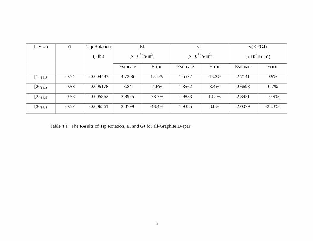
The estimated results of the tip rotation, the EI and GJ properties for the all-graphite D-spar and the all-glass D-spar cases are tabulated in Table 4.1 and 4.2respectively. The results indicate that EI decreases and GJ increases as the ply orientationangle increases (between 15° and 30°). The results also indicate that it is not possible toachieve the specified EI and GJ with a single ply orientation lay up. The best laminate layup that is close to the design criteria is the all-graphite case with 20° ply orientation.

It is possible to fulfill the EI and GJ requirements by replacing some of theunidirectional plies with a combination of angle plies, 0° and 90° ply orientation. Atypical example is shown in Table 4.2. The lay up of [2526/033]S for all-glass D-sparprovides a single-digit percentage error in EI and GJ. However, the tip rotation is reducedto half (from –0.002787°/lb to –0.001245°/lb) as the α interaction parameter has beenreduced from 0.43 to 0.19. The reduction of the α interaction parameter is caused by theinclusion of the orthotropic layers.

Therefore, in designing the D-spar, we need to relax the EI and GJ requirementsand maximize the tip rotation by maximizing value of the α interaction parameter. Thenext consideration for the D-spar design is structural integrity.

4.4 D-Spar Structural Integrity

One of the factors to consider in the structural analysis is the type of loadingexerted on the structure. In the current design, we focus our analysis only on cantileveredloading.

47

4.4.1 D-spar Modelling Using 3D-Beam Program

We need to mention some features about the 3D Beam program. The failurecriteria used in the 3D Beam software are based on the Tsai-Wu12 quadratic failurecriteria. If the strength/stress index (R) is greater than one, then the structure is safe. Requals 1 when the allowable or ultimate stress is reached.

The 3D Beam software outputs the distribution of the R along the cross-section atvarious longitudinal locations. Since we are analysing a constant cross-section D-spar,which has constant structural properties (EI, GJ), the failure should occur at the rootsection of a built-in structure. Therefore, only the output at the root (Element GroupNumber 1 as in 3D Beam notation) of the D-spar is presented.

The pin-point location of the failure at any cross-section is identified by the“brick” where the R index is less than or equal to one (or the lowest R value on the cross-section that is used to predict the failure load). The D-spar has been modelled with 26Bricks (Brick No. 1 to 26) for every cross-section at various longitudinal stations. And 4additional Bricks (Brick No. 27 to 30) are used to model the butt joint at the mid-planesection. The brick numbers of the D-spar are shown in Figure 4.2.

4.4.2 D-Spar Structural Analysis

Butt Joint

The selection of laminate schedule at the butt-joint layers depends on the strengthof the joint and the effect of these additional layers on the EI, GJ and α. We look intofour common sets of ply lay-up; i.e. [0/90], [+/-30], [+/-45], [+/-60]. The effects of thebutt joint reinforcement on the EI, GJ and α are shown in Tables 4.3 and 4.4 for the all-graphite and the all-glass D-spars respectively. The results indicate the additional layersat the joint do not significantly change D-spar structural properties.

The [0°/90°] ply lay-up for these additional layers at the joint is the best selectionbecause of the highest factor of safety (FS is similar to the R index). Therefore [0°/90°]ply lay-up is used for the ply layers at the joint.

Body

Three different D-spars have been studied, and the results are summarized insubsequent paragraphs.

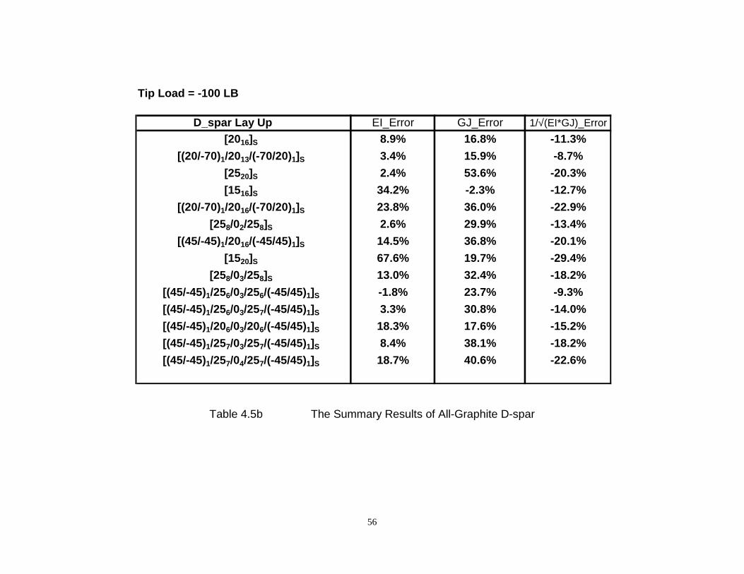
Tables 4.5a & 4.5b show the summarized results for the all-graphite D-spar. Theresults indicate that the [20°16] off-axis unidirectional ply gives the highest tip rotation.For a tip load of 420 lb., the tip rotation is about 1.9° at the factor of safety (or the Rindex) of 2. In addition, the EI and GJ errors are within 10% and 20% respectively.

Tables 4.6a & 4.6b show the summarized results for the all-glass D-spar. Theresults indicate the all [25°60] off axis unidirectional ply gives the highest tip rotation perunit pound load. The EI and GJ errors are –22.9% and 41.7% respectively, but the error

48

of 1/√(EI*GJ) is less than 5%. At safety factor of 2, the tip rotation and tip load of the[25°60] configuration are at 2.2° and 725 lb. respectively

Tables 4.7a & 4.7b show the summarized results for the hybrid D-spar. Theresults indicate the best laminate lay up for the hybrid D-spar is the combination of glassand graphite at the [20°] off-axis unidirectional ply because the α interaction parameter isbetween 0.5-0.56, and the error of the EI is less than 10%. The ratio of the mixture shouldbe one layer of glass material with two layers of graphite material.

4.5 D-Spar Configuration for Demonstration

The above analysis implies that the best laminate lay up to achieve the maximumtip rotation, as well as not to compromise the structural integrity, is 20°-25° off-axisunidirectional lay up. This lay up has one major disadvantage; the failure is catastrophicfailure. Since the same D-spars will undergo both the static test and modal test, it is betterto design the D-spars to fail at the first outer layer under static load. The D-spars are thendesigned for first-ply failure.

The following configurations are studied,

(i) Case a: the all-graphite D-spar ([θ1/2015/θ1]S)

(ii) Case b: the all-glass D-spar ( [θ1/2560/θ1]S)

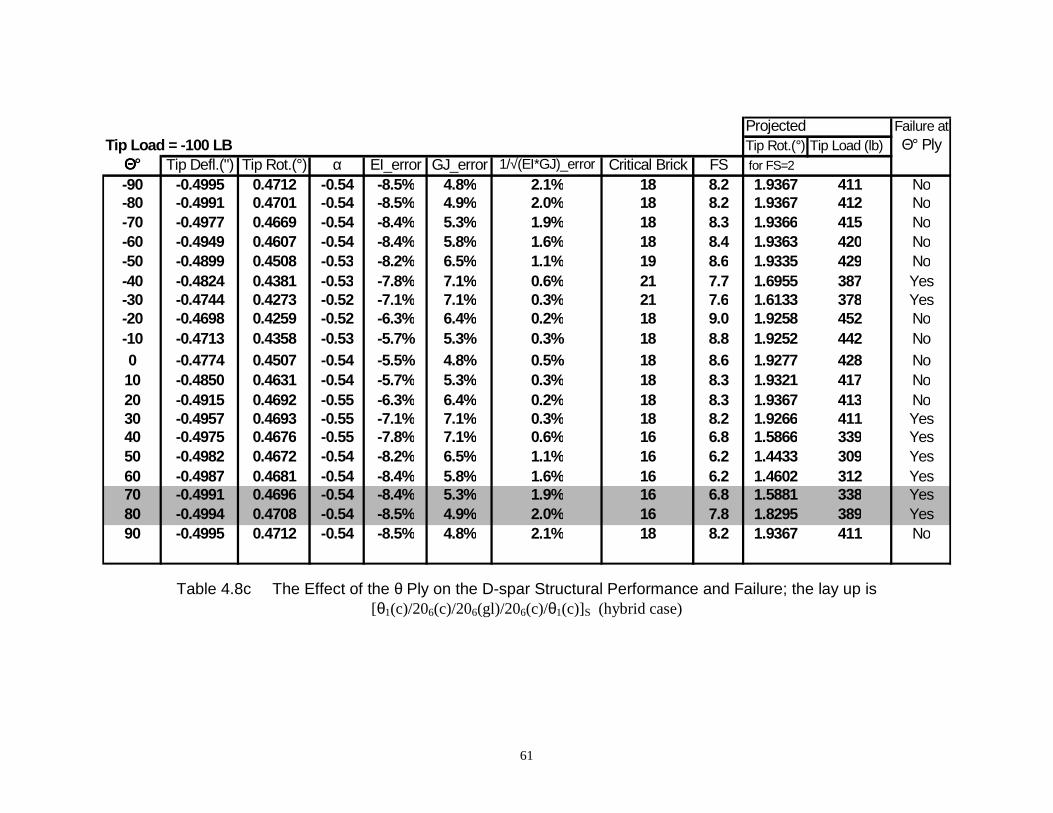
(iii) Case c: the hybrid D-spar ([θ1(c)/206(c)/206(gl)/206(c)/θ1(c)]S; ‘c’denotes graphite and ‘gl’ denotes glass)

Tables 4.8a, 4.8b and 4.8c show the summarized results for cases (a), (b) and (c)respectively. The results indicate the θ angle of the first-ply, which will fail first, shouldbe between,

(i) 60° and 70° [case (a)],

(ii) –50° and –60° [case (b)], and

(iii) 70° and 80° [case (c)].

4.6 Summary

To achieve the maximum tip rotation per unit pound load, the ply orientation ofthe laminate should be at 20° for the all-graphite D-spar and at 25° for the all-glass D-spar. The hybrid D-spar will have higher tip rotation if the mixture is one layer of theglass material to two layers of the graphite material. It is not possible to have the bendingand torsion stiffness of the D-spar close to the design values by just using one off-axisunidirectional lay up. The inclusion of non-anisotropic layers helps to meet the stiffness

49

criteria but fails to fulfill the requirement of the maximum tip rotation. The analysisindicates that the D-spar will be able to achieve at least 1° tip rotation without structurefailure under static tip loading.

50

-8.0

-7.0

-6.0

-5.0

-4.0

-3.0

-2.0

-1.0

0.0-0.8 -0.7 -0.6 -0.5 -0.4 -0.3 -0.2 -0.1 0

αααα

Tip

Roa

tion

( x 1

0 -3

° / l

b )

EI = 4.027E7 lb-in2

GJ = 1.795E7 lb-in2

D-spar Length (in) = 72

All "Glass" D-spar

All "Graphite" D-spar

Figure 4.1 The Tip Rotation Variation of a D-spar Exhibiting Specified StructuralProperties but Different α

Element Group #1

1-1.5

-1

-0.5

0

0.5

1

1.5

-3 -2 -1 0 1 2 3 4

X2

X3

21

3

4

5

6

7

8

9101112131415

16

17

18

19

20

21

22 23 24 25 26

27

28

30

29

Figure 4.2 The Modeling of D-spar Cross-Section with 30 "Brick" Elements

51

EI

(x 107 lb-in2)

GJ

(x 107 lb-in2)

√(EI*GJ)

(x 107 lb-in2)

Lay Up α Tip Rotation

(°/lb.)

Estimate Error Estimate Error Estimate Error

[1514]S -0.54 -0.004483 4.7306 17.5% 1.5572 -13.2% 2.7141 0.9%

[2014]S -0.58 -0.005178 3.84 -4.6% 1.8562 3.4% 2.6698 -0.7%

[2514]S -0.58 -0.005862 2.8925 -28.2% 1.9833 10.5% 2.3951 -10.9%

[3014]S -0.57 -0.006561 2.0799 -48.4% 1.9385 8.0% 2.0079 -25.3%

Table 4.1 The Results of Tip Rotation, EI and GJ for all-Graphite D-spar

52

EI

(x 107 lb-in2)

GJ

(x 107 lb-in2)

√(EI*GJ)

(x 107 lb-in2)

Lay Up α Tip Rotation

(°/lb.)

Estimate Error Estimate Error Estimate Error

[1564]S -0.35 -0.002183 4.2937 6.6% 2.1161 17.9% 3.0143 12.1%

[2064]S -0.41 -0.002553 3.8392 -4.7% 2.4335 35.6% 3.0566 13.7%

[2564]S -0.43 -0.002787 3.3135 -17.7% 2.7084 50.9% 2.9957 11.4%

[2526/033]S -0.19 -0.001245 3.8742 -3.8% 1.9125 6.5% 2.7220 1.2%

[3064]S -0.43 -0.002905 2.7781 -31.0% 2.8806 60.5% 2.8289 5.2%

Table 4.2 The Results of Tip Rotation, EI and GJ for all-Glass D-spar

53

Table 4.3 The Effect of the Ply Orientation of the Butt Joints for the all-graphite D-spar ( [(45/-45)1/257/04/257/(-45/45)1]S ).

Tip Load = -100 LBTip Defl.(") Tip Rot.(°) α EI_error GJ_error 1/sqrt(EI*GJ) Error Critical Brick FS

W/O Butt Joint Reinforcement -0.3356 0.2868 -0.42 18.16% 30.64% -19.51% 21 9.15Butt Joint Reinforcement

(0/90)8 -0.3279 0.2625 -0.40 18.69% 40.58% -22.58% 21 9.82(30/-30)8 -0.3199 0.2299 -0.38 18.51% 58.25% -26.98% 21 10.88(45/-45)8 -0.3241 0.2440 -0.39 18.30% 50.35% -25.02% 21 10.39(60/-60)8 -0.3273 0.2557 -0.40 18.24% 44.35% -23.46% 21 10.02

Safety Factor for the Bricks (27, 28, 29 and 30 ) at the butt jointBrick No 27 28 29 30

(0/90)8 35.04 30.44 25.45 28.56(30/-30)8 13.58 17.79 14.05 11.28(45/-45)8 15.57 16.83 13.60 12.76(60/-60)8 21.09 19.46 16.01 17.09

54

Table 4.4 The Effect of the Ply Orientation of the Butt Joints for the all-glass D-spar ([(45/-45)2/2515/034/2515/(-45/45)2]S

Tip Load = -100 LBTip Defl.(") Tip Rot.(°) α EI_error GJ_error 1/sqrt(EI*GJ) Error Critical Brick FS

W/O Butt Joint Reinforcement -0.3028 0.1038 -0.19 8.16% 30.18% -15.73% 16 18.03Butt Joint Reinforcement

(0/90)8 -0.3018 0.1000 -0.19 8.27% 35.23% -17.36% 16 18.51(30/-30)8 -0.3012 0.0969 -0.18 8.26% 39.74% -18.70% 16 18.90(45/-45)8 -0.3014 0.0974 -0.18 8.22% 39.12% -18.50% 16 18.84(60/-60)8 -0.3017 0.0988 -0.18 8.20% 37.11% -17.90% 16 18.66

Safety Factor for the Bricks (27, 28, 29 and 30 ) at the butt jointBrick No. 27 28 29 30(0/90)8 167.19 78.04 58.64 86.43

(30/-30)8 58.04 71.46 32.72 29.50(45/-45)8 67.50 52.65 26.99 30.52(60/-60)8 116.69 51.19 29.65 45.18

55

Table 4.5a The Summary Results of All-Graphite D-spar

Tip Load = -100 LB ProjectedTip Rot.(°) Tip Load (lb)

D_spar Lay Up Tip Rot.(°) α Critical Brick FS for FS=2

[2016]S 0.4615 -0.58 18 8.40 1.9380 420[(20/-70)1/2013/(-70/20)1]S 0.4375 -0.56 18 8.83 1.9323 442

[2520]S 0.4286 -0.59 18 7.91 1.6959 396[1516]S 0.4003 -0.54 18 11.37 2.2746 568

[(20/-70)1/2016/(-70/20)1]S 0.3792 -0.56 18 10.16 1.9260 508[258/02/258]S 0.3592 -0.51 18 9.21 1.6531 460

[(45/-45)1/2016/(-45/45)1]S 0.3414 -0.52 21 7.49 1.2783 374[1520]S 0.3296 -0.55 18 13.73 2.2636 687

[258/03/258]S 0.3090 -0.48 18 10.54 1.6292 527[(45/-45)1/256/03/256/(-45/45)1]S 0.2620 -0.40 21 8.84 1.1586 442[(45/-45)1/256/03/257/(-45/45)1]S 0.2570 -0.41 21 9.09 1.1687 455[(45/-45)1/206/03/206/(-45/45)1]S 0.2564 -0.42 21 9.33 1.1955 466[(45/-45)1/257/03/257/(-45/45)1]S 0.2526 -0.42 21 9.33 1.1781 466[(45/-45)1/257/04/257/(-45/45)1]S 0.2223 -0.40 21 10.44 1.1606 522

56

Table 4.5b The Summary Results of All-Graphite D-spar

Tip Load = -100 LB

D_spar Lay Up EI_Error GJ_Error 1/√(EI*GJ)_Error[2016]S 8.9% 16.8% -11.3%

[(20/-70)1/2013/(-70/20)1]S 3.4% 15.9% -8.7%[2520]S 2.4% 53.6% -20.3%[1516]S 34.2% -2.3% -12.7%

[(20/-70)1/2016/(-70/20)1]S 23.8% 36.0% -22.9%[258/02/258]S 2.6% 29.9% -13.4%

[(45/-45)1/2016/(-45/45)1]S 14.5% 36.8% -20.1%[1520]S 67.6% 19.7% -29.4%

[258/03/258]S 13.0% 32.4% -18.2%[(45/-45)1/256/03/256/(-45/45)1]S -1.8% 23.7% -9.3%[(45/-45)1/256/03/257/(-45/45)1]S 3.3% 30.8% -14.0%[(45/-45)1/206/03/206/(-45/45)1]S 18.3% 17.6% -15.2%[(45/-45)1/257/03/257/(-45/45)1]S 8.4% 38.1% -18.2%[(45/-45)1/257/04/257/(-45/45)1]S 18.7% 40.6% -22.6%

57

Table 4.6a The Summary Results of All-Glass D-spar

Table 4.6b The Summary Results of All-Glass D-spar

Tip Load = -100 LB ProjectedTip Rot.(°) Tip Load (lb)

D_spar Lay Up Tip Rot.(°) α Critical Brick FS for FS=2

[2560]S 0.2965 -0.43 18 14.5 2.1506 725[2060]S 0.2716 -0.41 18 18.5 2.5120 925

[01/2064/01]S 0.2385 -0.40 18 20.9 2.4931 1045[2017/1530/2017]S 0.2332 -0.38 18 21.1 2.4548 1053

[1560]S 0.2322 -0.35 18 25.4 2.9510 1271[(45/-45)2/2515/034/2515/(-45/45)2]S 0.1000 -0.19 16 18.5 0.9266 927

Tip Load = -100 LB

D_spar Lay Up Tip Rot.(°) EI_Error GJ_Error 1/√(EI*GJ)_Error[2560]S 0.2965 -22.9% 41.7% -4.3%[2060]S 0.2716 -10.7% 27.4% -6.3%

[01/2064/01]S 0.2385 -0.8% 38.1% -14.6%[2017/1530/2017]S 0.2332 2.1% 29.3% -13.0%

[1560]S 0.2322 -0.1% 10.8% -5.0%[(45/-45)2/2515/034/2515/(-45/45)2]S 0.1000 8.3% 35.2% -17.4%

58

Table 4.7a The Summary Results of Hybrid D-spar

Table 4.7b The Summary Results of Hybrid D-spar

Tip Load = -100 LB ProjectedTip Rot.(°) Tip Load (lb)

D_spar Lay Up Tip Rot.(°) α Critical Brick FS for FS=2

[207(c)/02(gl)/207(c)]S 0.4717 -0.56 18 8.2 1.9298 409[01(gl)/206(c)/206(gl)/206(c)/01(gl)]S 0.4507 -0.54 18 8.5 1.9256 427

[208(c)/02(gl)/207(c)]S 0.4471 -0.56 18 8.6 1.9284 431[01(gl)/205(c)/2020(gl)/205(c)/01(gl)]S 0.3598 -0.50 18 10.6 1.9076 530

[(45/-45)2(gl)/257(c)/014(gl)/257(c)/(-45/45)2(gl)]S 0.2481 -0.42 16 10.7 1.3326 537

Tip Load = -100 LB

D_spar Lay Up Tip Rot.(°) EI_Error GJ_Error 1/√(EI*GJ)_Error[207(c)/02(gl)/207(c)]S 0.4717 -0.8% 6.0% -2.4%

[01(gl)/206(c)/206(gl)/206(c)/01(gl)]S 0.4507 -5.5% 4.8% 0.5%[208(c)/02(gl)/207(c)]S 0.4471 6.0% 12.7% -8.5%

[01(gl)/205(c)/2020(gl)/205(c)/01(gl)]S 0.3598 1.8% 20.0% -9.6%[(45/-45)2(gl)/257(c)/014(gl)/257(c)/(-45/45)2(gl)]S 0.2481 3.4% 46.6% -18.8%

Note : "gl" denotes glass and "c" denotes graphite

59

Projected Failure atTip Load = -100 LB Tip Rot.(°) Tip Load (lb) Θ° Ply

ΘΘΘΘ° Tip Defl.(") Tip Rot.(°) α EI_error GJ_error 1/√(EI*GJ)_error Critical Brick FS for FS=2-90 -0.4558 0.4487 -0.56 3.3% 15.1% -8.3% 18 8.6 1.9399 432 No-80 -0.4540 0.4451 -0.56 3.3% 15.3% -8.4% 18 8.7 1.9394 436 No-70 -0.4504 0.4375 -0.56 3.4% 15.9% -8.7% 18 8.9 1.9386 443 No-60 -0.4435 0.4239 -0.55 3.7% 17.0% -9.2% 18 9.1 1.9371 457 No-50 -0.4313 0.4005 -0.53 4.3% 18.9% -10.2% 21 7.6 1.5127 378 Yes-40 -0.4098 0.3630 -0.51 5.9% 21.5% -11.8% 21 6.1 1.1022 304 Yes-30 -0.3773 0.3133 -0.47 9.4% 24.1% -14.2% 21 5.7 0.8858 283 Yes-20 -0.3447 0.2776 -0.44 15.7% 23.4% -16.3% 21 7.2 0.9939 358 Yes-10 -0.3371 0.2951 -0.46 21.1% 18.2% -16.4% 18 12.7 1.8716 634 No0 -0.3575 0.3536 -0.52 22.8% 15.1% -15.9% 18 10.7 1.8897 534 No10 -0.3896 0.4097 -0.56 21.1% 18.2% -16.4% 18 9.4 1.9173 468 No20 -0.4214 0.4378 -0.58 15.7% 23.4% -16.3% 18 8.8 1.9338 442 Yes30 -0.4420 0.4428 -0.58 9.4% 24.1% -14.2% 18 6.9 1.5190 343 Yes40 -0.4507 0.4433 -0.57 5.9% 21.5% -11.8% 18 6.9 1.5190 343 Yes50 -0.4541 0.4451 -0.57 4.3% 18.9% -10.2% 16 7.2 1.5959 359 Yes60 -0.4557 0.4476 -0.56 3.7% 17.0% -9.2% 16 7.4 1.6608 371 Yes70 -0.4564 0.4494 -0.56 3.4% 15.9% -8.7% 16 8.0 1.7872 398 Yes80 -0.4565 0.4500 -0.56 3.3% 15.3% -8.4% 18 8.6 1.9406 431 No90 -0.4559 0.4490 -0.56 3.3% 15.1% -8.3% 18 8.6 1.9400 432 No

Table 4.8a The Effect of the θ Ply on the D-spar Structural Performance and Failure; the lay up is [θ1/2015/θ1]S (allgraphite case)

60

Table 4.8b The Effect of the θ Ply on the D-spar Structural Performance and Failure; the lay up is [θ1/2560/θ1]S (all glasscase)

Projected Failure atTip Load = -100 LB Tip Rot.(°) Tip Load (lb) Θ° Ply

ΘΘΘΘ° Tip Defl.(") Tip Rot.(°) α EI_error GJ_error 1/√(EI*GJ)_error Critical Brick FS for FS=2-90 -0.4942 0.2864 -0.42 -22.1% 44.3% -5.7% 11 8.2 1.1683 408 Yes-80 -0.4940 0.2860 -0.42 -22.1% 44.4% -5.7% 11 9.0 1.2823 448 Yes-70 -0.4933 0.2845 -0.42 -22.0% 44.7% -5.9% 11 10.6 1.5126 532 Yes-60 -0.4916 0.2816 -0.42 -22.0% 45.3% -6.1% 11 13.9 1.9543 694 Yes-50 -0.4883 0.2767 -0.41 -21.8% 46.0% -6.4% 19 13.7 1.8902 683 Yes-40 -0.4829 0.2700 -0.41 -21.4% 46.6% -6.8% 21 11.5 1.5577 577 Yes-30 -0.4759 0.2635 -0.40 -20.7% 46.6% -7.2% 21 10.6 1.3947 529 Yes-20 -0.4704 0.2617 -0.40 -19.9% 45.8% -7.5% 21 13.1 1.7119 654 Yes-10 -0.4692 0.2661 -0.41 -19.3% 44.8% -7.5% 18 16.0 2.1353 802 No0 -0.4721 0.2739 -0.41 -19.1% 44.3% -7.5% 18 15.6 2.1401 781 No10 -0.4775 0.2815 -0.42 -19.3% 44.8% -7.5% 18 15.2 2.1464 762 No20 -0.4838 0.2863 -0.43 -19.9% 45.8% -7.5% 18 15.0 2.1520 752 No30 -0.4891 0.2876 -0.43 -20.7% 46.6% -7.2% 18 12.9 1.8563 646 Yes40 -0.4922 0.2868 -0.43 -21.4% 46.6% -6.8% 16 9.9 1.4158 494 Yes50 -0.4935 0.2860 -0.42 -21.8% 46.0% -6.4% 16 8.4 1.2027 421 Yes60 -0.4939 0.2858 -0.42 -22.0% 45.3% -6.1% 16 8.0 1.1423 400 Yes70 -0.4941 0.2860 -0.42 -22.0% 44.7% -5.9% 11 7.9 1.1309 395 Yes80 -0.4942 0.2864 -0.42 -22.1% 44.4% -5.7% 11 7.8 1.1167 390 Yes90 -0.4942 0.2864 -0.42 -22.1% 44.3% -5.7% 11 8.1 1.1604 405 Yes

61

Projected Failure atTip Load = -100 LB Tip Rot.(°) Tip Load (lb) Θ° Ply

ΘΘΘΘ° Tip Defl.(") Tip Rot.(°) α EI_error GJ_error 1/√(EI*GJ)_error Critical Brick FS for FS=2-90 -0.4995 0.4712 -0.54 -8.5% 4.8% 2.1% 18 8.2 1.9367 411 No-80 -0.4991 0.4701 -0.54 -8.5% 4.9% 2.0% 18 8.2 1.9367 412 No-70 -0.4977 0.4669 -0.54 -8.4% 5.3% 1.9% 18 8.3 1.9366 415 No-60 -0.4949 0.4607 -0.54 -8.4% 5.8% 1.6% 18 8.4 1.9363 420 No-50 -0.4899 0.4508 -0.53 -8.2% 6.5% 1.1% 19 8.6 1.9335 429 No-40 -0.4824 0.4381 -0.53 -7.8% 7.1% 0.6% 21 7.7 1.6955 387 Yes-30 -0.4744 0.4273 -0.52 -7.1% 7.1% 0.3% 21 7.6 1.6133 378 Yes-20 -0.4698 0.4259 -0.52 -6.3% 6.4% 0.2% 18 9.0 1.9258 452 No-10 -0.4713 0.4358 -0.53 -5.7% 5.3% 0.3% 18 8.8 1.9252 442 No0 -0.4774 0.4507 -0.54 -5.5% 4.8% 0.5% 18 8.6 1.9277 428 No10 -0.4850 0.4631 -0.54 -5.7% 5.3% 0.3% 18 8.3 1.9321 417 No20 -0.4915 0.4692 -0.55 -6.3% 6.4% 0.2% 18 8.3 1.9367 413 No30 -0.4957 0.4693 -0.55 -7.1% 7.1% 0.3% 18 8.2 1.9266 411 Yes40 -0.4975 0.4676 -0.55 -7.8% 7.1% 0.6% 16 6.8 1.5866 339 Yes50 -0.4982 0.4672 -0.54 -8.2% 6.5% 1.1% 16 6.2 1.4433 309 Yes60 -0.4987 0.4681 -0.54 -8.4% 5.8% 1.6% 16 6.2 1.4602 312 Yes70 -0.4991 0.4696 -0.54 -8.4% 5.3% 1.9% 16 6.8 1.5881 338 Yes80 -0.4994 0.4708 -0.54 -8.5% 4.9% 2.0% 16 7.8 1.8295 389 Yes90 -0.4995 0.4712 -0.54 -8.5% 4.8% 2.1% 18 8.2 1.9367 411 No

Table 4.8c The Effect of the θ Ply on the D-spar Structural Performance and Failure; the lay up is[θ1(c)/206(c)/206(gl)/206(c)/θ1(c)]S (hybrid case)

62

Chapter 5

D-Spar Fabrication

In the previous chapter, the design of three D-spars was described. Only thehybrid D-spar and the all-carbon D-spar were fabricated. The fabrication of all-glass D-spar did not materialize because of budget constraints. The fabrication was done at theMaterial Research Laboratory, Industrial Technology Research Institute (ITRI) inTaiwan. The engineers of the laboratory are familiar with the bladder process and theyhave been using this process in sporting goods applications. The fabrication was jointlycarried out by a team composed of ITRI's engineers and researchers from StanfordUniversity.

The bladder process uses an inflatable mandrel to pressurize the laminate surface.The inflatable mandrel is inflated from an external source, and the pressure is transferredto the laminate panel surface. The laminate surface is pressed against a female mold to agive smooth surface finish.

In this chapter, we describe the tooling used in the D-spar fabrication, thefabrication process, and problems faced at the earlier stages of D-spar fabrication.

5.1 Tooling and Materials Used in D-Spar Fabrication

5.1.1 Materials

In previous chapters, we indicated T800/3900-2 Graphite/Epoxy material wasused in D-spar design. However a different category of Graphite/Epoxy material wasused in D-spar fabrication. The material used for D-spar fabrication wasTorayca/P3051F. The difference in ply properties of these materials is shown in Table5.1. There is not much difference in structural performance, as shown in Table 5.2.However, the manufactured D-spars are thicker than the designed one, because moreplies are added to compensate for axial ply stiffness reduction (see Table 5.2).

5.1.2 Tooling

There are two types of tooling used in D-spar fabrication. A wooden mold wasused for the lay-up process, and a hard female mold was used to produce a smoothsurface finish.

5.1.2.1 Wooden Mold

The shape of the wooden mold is similar to that of the D-spar, and the dimensionof the wooden mold is close to the D-spar internal dimension. However the D-sparinternal dimension depends on skin thickness. The average skin thickness of the hybrid

63

D-spar and the all carbon D-spar is 0.14 inches and 0.13 inches respectively. The woodenmold was sized based on the internal dimension of the hybrid D-spar.

5.1.2.2 Female Tooling

The female tooling consists of four parts. They are two end plates, one base plateand one U-shaped plate (see Figure 5.1). The length of the base plate and U-shaped plateis about 82 inches.

5.2 Fabrication Process

The whole fabrication process can be broken into five stages.

5.2.1 Pre-Lay-up Preparation

At this stage, the pre-impregnated aligned fibers (called prepregs) are sized to thecorrect length, width and ply orientation according to the laminate schedule of therespective D-spar. Tables 5.3 and 5.4 show the laminate schedule of the hybrid and theall-carbon D-spars respectively. The width of prepregs is determined by the amount ofoverlap and the D-spar half-circumference length. The last step of this stage is to arrangethe prepared prepregs into two stacks at each side of the wooden mold. The stackingsequence of the prepregs of each pile is according to the laminate schedule for the lay-up.

5.2.2 Lay-up

The steps are

a. Make markings at both ends of the wooden mold as shown in Figure 5.2.Each marking is about 1 cm. The marking is to facilitate the formation ofthe staggered overlap joint.

b. Wrap the wooden mold with a sheet of peel ply. This peel ply separatesthe wooden mold from the laminate and facilitates the removal of thewooden mold before the assembly of female tooling.

c. Lay the prepregs onto the wooden mold according to the laminateschedule (see Table 5.3 and 5.4). A long ruler is used to facilitate the lay-up (see Figure 5.3).

5.2.3 Inflatable Bag Preparation

The steps are:

a. Select a nylon bag that is slightly larger than the size of the D-spar.

b. Cut the bag at a length 6 inches more than the fabricated D-spar length.

64

c. Seal one end of the bag and fold the sealed end inward. The inwardfolding is a critical step. As the bag is being pressurized, the inwardfolding of the sealed end causes this end to push outward instead ofexpanding outward.

d. Attach a rubber nozzle to the other end of the bag (see Figure 5.4a). Thesealing is done by wrapping a string of prepregs and shrinkage tape (seeFigure 5.4b).

5.2.4 Assembly

The steps are

a. Clean the two end-plates, base plate and U-shaped plate. Spray releaseagent on all surfaces of the plates.

b. Turn the U-shaped plate with the legs pointing upward.

c. Transfer the wooden mold (with uncured D-spar) to the U-shaped tooling.

d. Remove the wooden mold from the uncured D-spar (see Figure 5.5).

e. Insert the bag into the hollow section.

f. Attach both ends with a set of [±45°2]T laminate (see Figure 5.6). This isto avoid physical contact between the nylon bag and the two end-plates.

g. Assemble the base plate and two end-plates. After the assembly, theuncured D-spar is enclosed, and the rubber nozzle remains outside.

h. Supply slight pressure to the bag through the nozzle and check for airleakage.

5.2.5 Curing

The whole assembly is then transferred to an oven for curing (see Figure 5.7). Thecuring steps are

a. Connect the nozzle to an air compressor unit.

b. Set the pressure to 85-90 MPa.

c. Set the oven temperature according to the curing cycle (see Figure 5.8).

65

5.3 Earlier Phase Fabrication Problems

Seven D-spars were made. Table 5.5 shows the order of the D-spar beingfabricated and the condition of each D-spar. The first and second D-spars were the 8-layer all-carbon D-spars. This was to check and fine-tune the fabrication process. Therewas problem on removing the first 8-layer all-carbon D-spar. The U-shaped plate wasmodified with the legs opened outward by 1.9° in order to remove the D-spar from thetooling. Therefore, the cross-section of the fabricated D-spar is different from the designone (see Figure 5.11). The third and fourth D-spars have surface imperfection problems,and both D-spars are also not symmetric (see Figure 5.9) with reference to the mid-plane.The sixth D-spar was damaged because of a leakage of the bag during curing. The fifthand seventh D-spars were successfully fabricated with good surface finish and therequired symmetry (see Figure 5.10). The fifth D-spar made is the hybrid D-spar, and theseventh is the all-carbon one. The surface imperfections and the non-symmetry problemsmay be related. The problem on non-symmetry D-spar was fixed by having a symmetriclay-up at the joints (staggered overlap joint). No surface imperfections were observedafter fixing the non-symmetry problem.

5.4 Staggered Overlap Joint Design

One critical point in D-spar fabrication is the joint design. As mentioned earlier,the bend-twist coupled D-spar consists of two symmetric clamshells held together byeither a butt joint or an overlap joint. Both the butt joint and overlap joint designs werenot adopted in fabrication, as both designs have more disadvantages than the preferreddesign invented during the learning curve of the fabrication process. The new joint designis called staggered overlap joint design. Figure 5.12 shows the three possible jointdesigns. The disadvantages of a single overlap joint design are the thickness at the joint isdoubly thicker than the thickness at the main skin and the strength of the joint isweakened by step-change in thickness distribution. The butt joint design carries the samedisadvantages as those of the single overlap joint design and has an additionaldisadvantage of requiring more lay-up operation steps. The main advantages of thestaggered overlap joint are that the step-change in skin thickness surrounding the joint isreduced to a minimum and the joint is strengthened.

Tables 5.3 and 5.4 show the lay-up sequence for the hybrid and the all carbon D-spar respectively. The symmetry of the lay-up is clearly seen in both tables. In addition tothat, the number of ply layers near the mid-plane of the hybrid D-spar has been reducedfrom 56 (if a single overlap joint were used) to 39. Further away from the mid-plane, thenumber of ply layers reduce to 28. The stagger overlap joint design of the all-carbon D-spar is even better than that of the hybrid D-spar. At the mid-plane of the all-carbon D-spar, the number of ply layers is 34. Further away from the mid-plane, the number of plylayers reduces to 26.

66

Description T800/3900-2

(Graphite/Epoxy)

Torayca/P3051F

(Graphite/Epoxy)

Ex(msi) 23.2 17.5

Ey(msi) 1.3 1.3

Es(msi) 0.9 0.8

νx 0.28 0.3

Table 5.1 Ply Properties of T800/3900-2 and Torayca/P3051F.

67

Tip Load = -100 LB

D-Spar Material Laminate Schedule Tip Defl.(") Tip Rot. (°) α EI_error GJ_error 1/√EI*GJ_error Remark

Hybrid T800/3900-2 [70*/206/206*/206/70*] -0.499 0.470 -0.54 -8.4% 5.3% 1.9% *: glass

Hybrid Torayca/P3051F [70*/209/208*/209/70*] -0.499 0.434 -0.51 -13.1% 3.5% 5.4% *: glass

Carbon T800/3900-2 [60/2515/60] -0.456 0.448 -0.56 3.7% 17.0% -9.2%

Carbon Torayca/P3051F [60/2524/60] -0.450 0.417 -0.54 0.0% 15.0% -6.8%

Table 5.2 Structural Performance of the Hybrid and the Carbon D-spars Made by Two Different Carbon Materials.

68

Lay from Wooden Mold's MarkingSequenceNo:

Layers ofPrepregs

Ply Orientation

(°)

Type of Material Prepregs Width

(cm) Left-Side Right-Side

1 1 70 Glass 22 0 -2

2 8 20 Carbon 22.1 0 -2

3 4 20 Glass 22.5 -2 -4

4 2 20 Carbon 22.7 1 -1

5 4 20 Glass 22.8 4 2

6 8 20 Carbon 23.0 2 0

7 1 70 Glass 23.4 2 0

Table 5.3 Lay-up Laminate Schedule for the Hybrid D-spar (see also Figure 5.2)

69

Lay from Wooden Mold's MarkingSequenceNo:

Layers ofPrepregs

Ply Orientation

(°)

Type of Material Prepregs Width

(cm) Left-Side Right-Side

1 1 60 Carbon 22 1 -1

2 6 20 Carbon 22.2 0 -2

3 6 20 Carbon 22.7 2 0

4 6 20 Carbon 23.1 -2 -4

5 6 20 Carbon 23.7 4 2

6 1 60 Carbon 23.8 1 -1

Table 5.4 Lay-up Laminate Schedule for the All-Carbon D-spar (see also Figure 5.2)

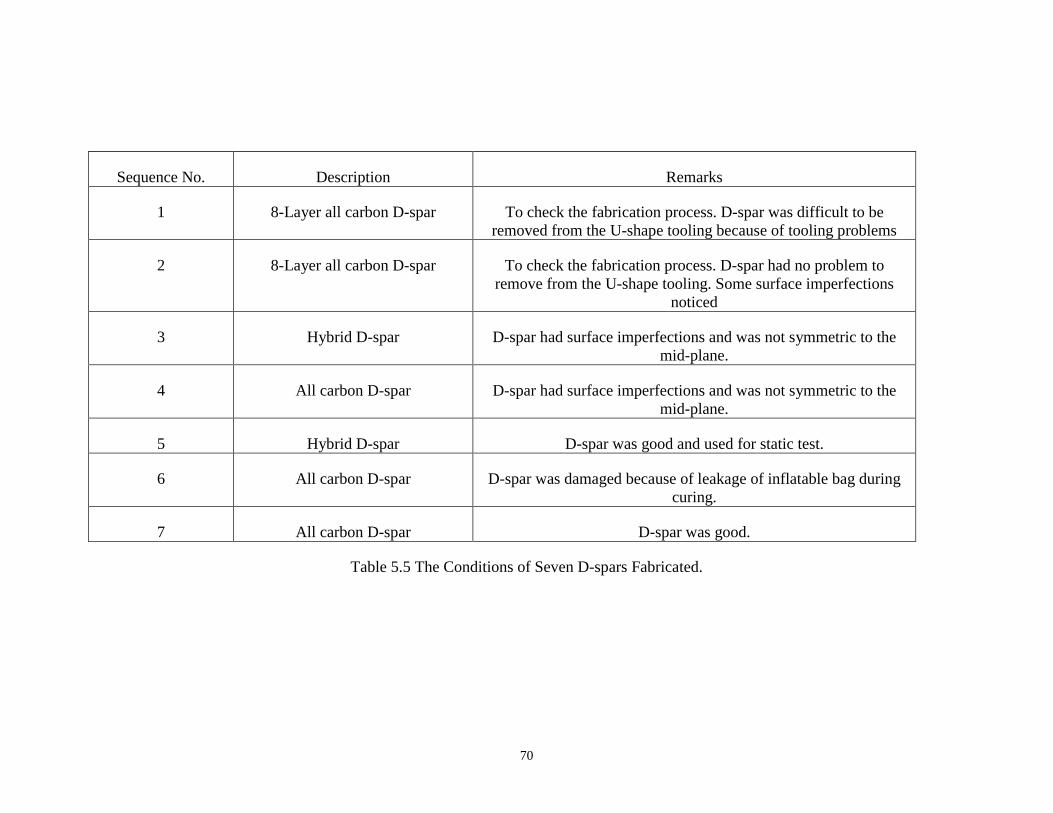
70

Sequence No. Description Remarks

1 8-Layer all carbon D-spar To check the fabrication process. D-spar was difficult to beremoved from the U-shape tooling because of tooling problems

2 8-Layer all carbon D-spar To check the fabrication process. D-spar had no problem toremove from the U-shape tooling. Some surface imperfections

noticed

3 Hybrid D-spar D-spar had surface imperfections and was not symmetric to themid-plane.

4 All carbon D-spar D-spar had surface imperfections and was not symmetric to themid-plane.

5 Hybrid D-spar D-spar was good and used for static test.

6 All carbon D-spar D-spar was damaged because of leakage of inflatable bag duringcuring.

7 All carbon D-spar D-spar was good.

Table 5.5 The Conditions of Seven D-spars Fabricated.

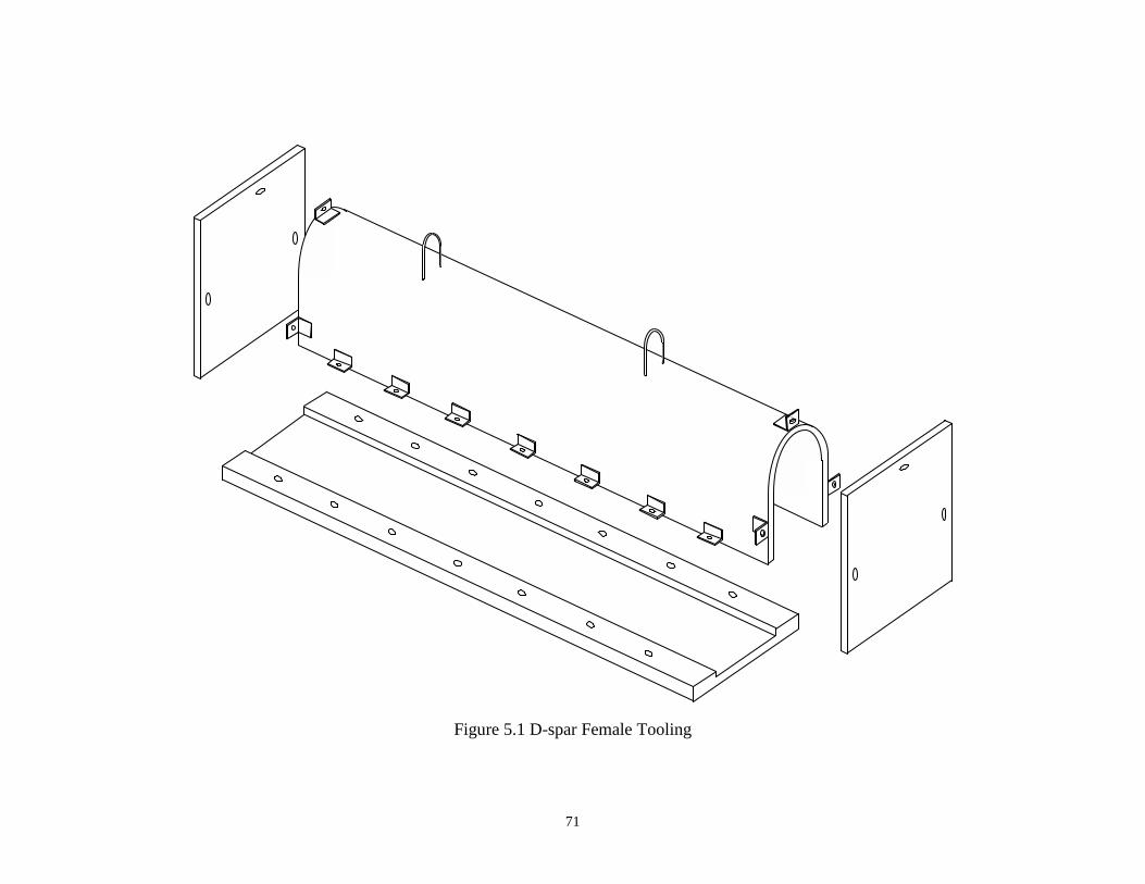
71

Figure 5.1 D-spar Female Tooling

72

-1-2

-3-4

0 1 23

4

RightLeft

Figure 5.2 End-Marking on Wooden Mold for the Lay-up.

Figure 5.3 A Long Ruler Used for the Alignment.

73

Figure 5.4a Place a Nozzle at the End of the Bag

Figure 5.4b Strings of Prepregs Wrapped around the Nozzle for Sealing

74

Figure 5.5 Remove the Wooden Mold Out of the Uncured D-spar

Figure 5.6 Protect Two Ends with a Sheet of [±45°2]T Laminate

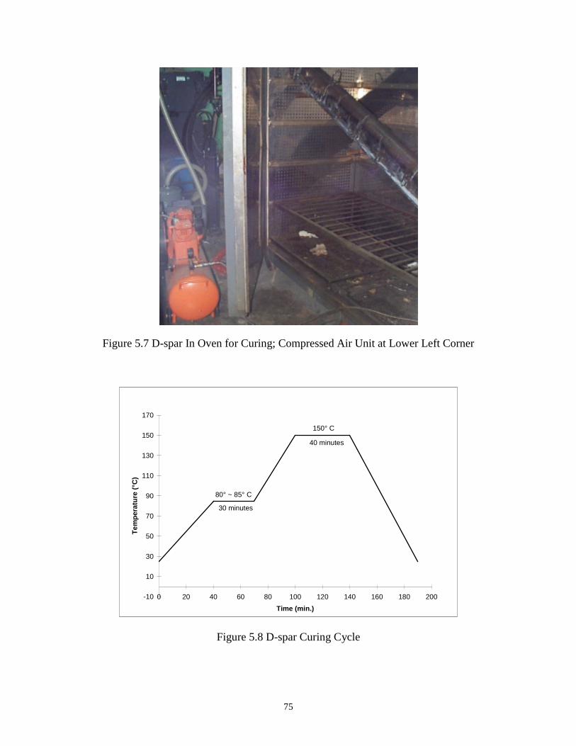
75

Figure 5.7 D-spar In Oven for Curing; Compressed Air Unit at Lower Left Corner

-10

10

30

50

70

90

110

130

150

170

0 20 40 60 80 100 120 140 160 180 200Time (min.)

Tem

pera

ture

(°C

)

80° ~ 85° C

150° C

30 minutes

40 minutes

Figure 5.8 D-spar Curing Cycle

76

Figure 5.9 The Non-symmetric D-spar

Figure 5.10 The Hybrid and All-Carbon D-spars

77

0.3"

0.15"

0.15"

1.9°

Figure 5.11 The Cross-Section Difference Between the Fabricated D-spar and the DesignOne

Wooden Mold

Overlap Joint(a)

-1-2-3

-4

0 1 23

4

(c)Staggered Joint

Wooden Mold

(b)

Wooden Mold

Butt Joint

Figure 5.12 Three Possible Joint Designs.

Chapter 6

Static & Modal Testing

Two D-spars were successfully fabricated. Only the hybrid D-spar of the twogood D-spars has been subjected to testing. The tests are the cantilever static test and themodal test. The static test was conducted at ITRI's testing facility, and the modal test wasdone at Sandia National Laboratories.

This chapter covers the static test set-up, the quality of the static test results, thecomparison between the test results and the numerical predictions, and the post-modaltest analysis.

6.1 Static Test Set-Up

The hybrid D-spar was subjected to the cantilever static test. The test set-up isshown in Figure 6.1. An aluminum block was inserted at the built-in end of the D-spar forreinforcement. The D-spar was then clamped tightly onto the test jig. The loads (deadweights were used) were applied vertically at the free end and were at a transversedistance 2.25" from the vertical wall of the D-spar (see Figures 6.2a and 6.2b). The deadweights were 5.84, 14.24, 21.04, 30.84, 37.04, 42.24, and 47.44 kg.

The measured parameters were vertical deflection, strains, and bend-inducedtwist. Displacement dial gauges were placed at locations x=56", 66" and 72" from thebuilt-in end to measure respective vertical deflection. Two cross-bars (about 12" long)were positioned at locations x=66" and 72" to determine the bend-induced twist (seeFigure 6.3). The strain gauges were attached at three longitudinal locations (see Figure6.4). Two single-strain gauges were placed at x=0" at the top and bottom flat-skins. ThreeRosettes were at x=6" (top and bottom skins) and at x=18" (top skin only).

6.2 Test Results

Each measured parameter was plotted against the loads, and a linear regressionmethod was used to curve-fit the data to obtain normalized parameters (per unit poundforce). Figures 6.5 and 6.6 show the vertical deflection measurements and the derivedbend-induced twist under various tip loads, respectively. The strains at three locations areshown in Figures 6.7, 6.8 and 6.9. The plots indicate that all results are linearly correlatedto loads except the bend-induced twist. The poor result on the bend-induced twistmeasurement may be due to inherent measurement error because the rotation is verysmall.

6.3 Comparison Between Estimated and Experimental Results

The normalized experimental results are compared to the results of two numericalmodels: 3D Beam and ANSYS models (the final geometry and material properties areused). Figures 6.10 to 6.14 show the vertical deflection, bend-induced twist, top skinlongitudinal strain (e1), transverse strain (e2) and shear strain (e6) comparisons,respectively. The hollow symbols in the graphs represent the experimental results dividedby the respective tip loads. The solid symbol in the figures represents the normalizedresults after linear curved fitting through the experimental results. The scatter of theexperimental results without linear curved fitting is clearly seen in those figures.

The comparisons between the experimental results and ANSYS results areexcellent except for results located near the ends of the D-spar. The ANSYS modelindicates that there are local deformation effects from the fixed boundary condition andapplied load. As for the case of the 3D-Beam model, the experimental results are higherthan the estimated results if no warping is included in the 3D-Beam model. The 3D-Beamestimated results are close to the test results once the torsion-related out-of-plane warpinghas been included. As observed in Figures 6.11 and Figure 6.14, torsion-related out-of-plane warping has a significant effect on the magnitude of bend-induced twist andtransverse shear. Both the twist angle and shear strain (e6) are nearly doubled if warpingis considered. The effect from warping tends to marginally increase the α estimate buthas significant effect on the bend-induced twist angle.

6.4 Post-Modal Testing Analysis

The modal testing was completed by Sandia National Laboratories13. This sectiondescribes the parameter sensitivity study done in order to reduce the discrepancy betweenthe experimental results and modal analysis results (ANSYS model).

Table 6.1 shows initial comparisons on modal frequencies between theexperimental results and ANSYS results. The initial frequency discrepancy is huge andthe minimum error is about 10%. The discrepancy is mainly because the D-spar was notfabricated to exact dimensions and the measured material properties are different fromthe specification. The dimensional deviation was discussed in Chapter 5. The differenceson material properties are reflected in Tables 6.2a and 6.2b. The main differences are onthe Ex modulus and the ply thickness.

The ANSYS model has been updated to include all the changes. The new resultsare shown in Table 6.3. Table 6.3 is not in the same order as Table 6.1; the beam modes,torsion modes and oval modes are re-grouped together for clarity. The percentage oferrors for the beam modes (Seq. No. 1-4) is less than 4%; for the torsion modes (Seq. No.5-7) less than 10% and for the oval modes (Seq. No. 9-14) less than 20%. To furtherreduce errors, especially those errors related to the beam and torsion modes, a parametersensitivity study was carried out.

The basic input to the ANSYS modal analysis model is the geometry of the D-spar, the ply properties, and the laminate schedule at every section (including the overlapregion) of the D-spar. The ply properties are the major uncertainty data input because thevolume fraction of the resin usually is unknown. Therefore, the sensitivity study mainlyfocuses on ply property variations. It is also expected that the adjustments to plyproperties are small, because the errors of the beam modes are less than 4%.

The adjustments are

a. reduction of Ex (both glass and graphite fibers) by a factor of 1.05,

b. increase of ply thickness (both glass and graphite fibers) by the samefactor of 1.05,

c. changing of ply orientation of the main skins from 20° to 20.5°.

The same adjustment factor is used for both (a) and (b). This is to keep the product of Exand ply thickness constant. By reducing Ex and increasing ply thickness by the sameamount we approximate the situation where the amount of fibers is known, but theamount of resin could vary.

Table 6.4 shows the comparisons for modal frequencies after the adjustments. Theimprovements are clearly seen on the first flatwise bending mode, the first twisting mode,the cross-section shear mode and the oval modes --- about a 3% improvement. Additionaladjustments are not required because the weight of the D-spar and the skin thickness areclose to the measured values (see bottom of Table 6.4). The first and second flatwisebending and torsion mode shapes for both the analytical model and modal test model areshown from Figures 6.15 to 6.18.

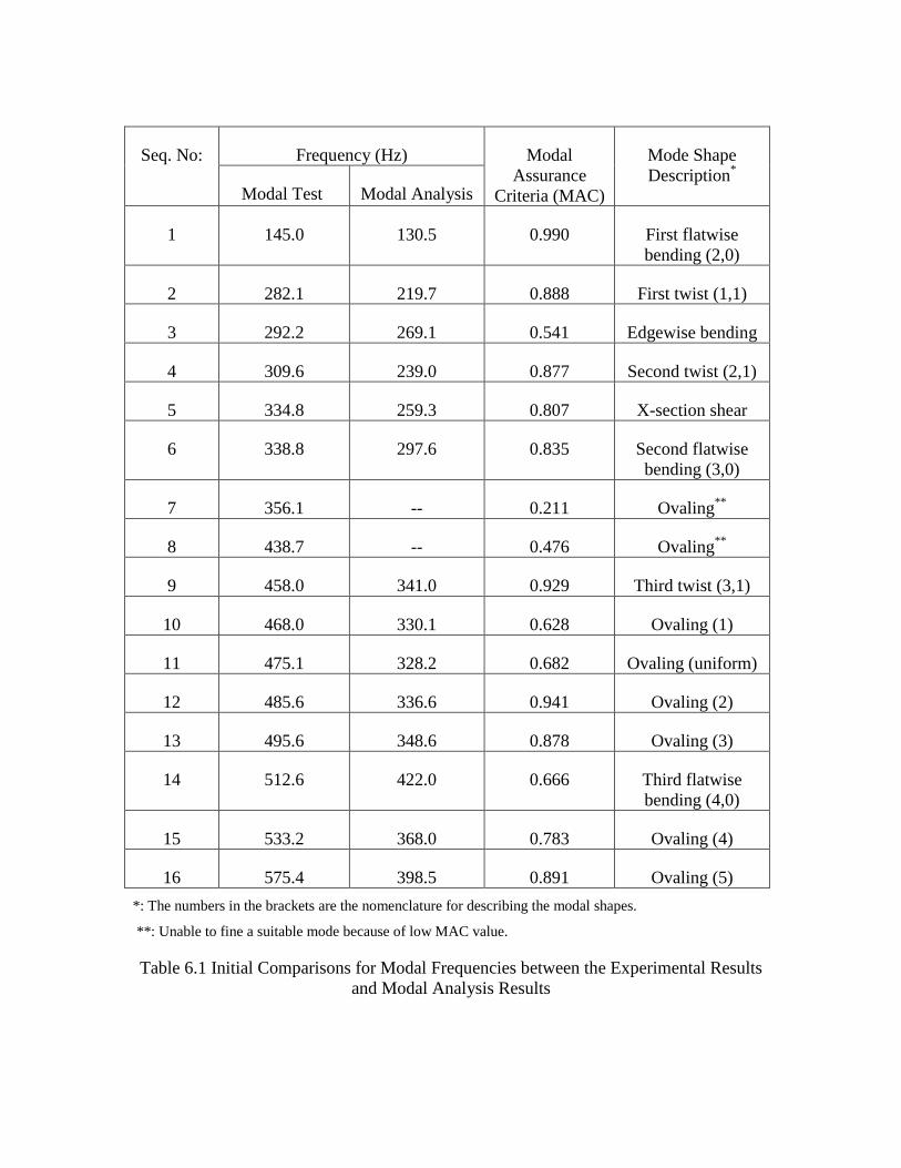
Frequency (Hz)Seq. No:

Modal Test Modal Analysis

ModalAssurance

Criteria (MAC)

Mode ShapeDescription*

1 145.0 130.5 0.990 First flatwisebending (2,0)

2 282.1 219.7 0.888 First twist (1,1)

3 292.2 269.1 0.541 Edgewise bending

4 309.6 239.0 0.877 Second twist (2,1)

5 334.8 259.3 0.807 X-section shear

6 338.8 297.6 0.835 Second flatwisebending (3,0)

7 356.1 -- 0.211 Ovaling**

8 438.7 -- 0.476 Ovaling**

9 458.0 341.0 0.929 Third twist (3,1)

10 468.0 330.1 0.628 Ovaling (1)

11 475.1 328.2 0.682 Ovaling (uniform)

12 485.6 336.6 0.941 Ovaling (2)

13 495.6 348.6 0.878 Ovaling (3)

14 512.6 422.0 0.666 Third flatwisebending (4,0)

15 533.2 368.0 0.783 Ovaling (4)

16 575.4 398.5 0.891 Ovaling (5)*: The numbers in the brackets are the nomenclature for describing the modal shapes.

**: Unable to fine a suitable mode because of low MAC value.

Table 6.1 Initial Comparisons for Modal Frequencies between the Experimental Resultsand Modal Analysis Results

Description Graphite/Epoxy Glass/Epoxy

Ex(msi) 17.5 5.6

Ey(msi) 1.3 1.2

Es(msi) 0.8 0.66

νx 0.28 0.3

Ply Thickness(inches)

0.00605 0.00496

Table 6.2a The Material Properties used for D-spars Design.

Description Graphite/Epoxy Glass/Epoxy

Ex(msi) 19.35 6.2

Ey(msi) 1.3 1.2

Es(msi) 0.7 0.60

νx 0.28 0.3

Ply Thickness(inches)

0.0055 0.00425

Table 6.2b The Measured Material Properties.

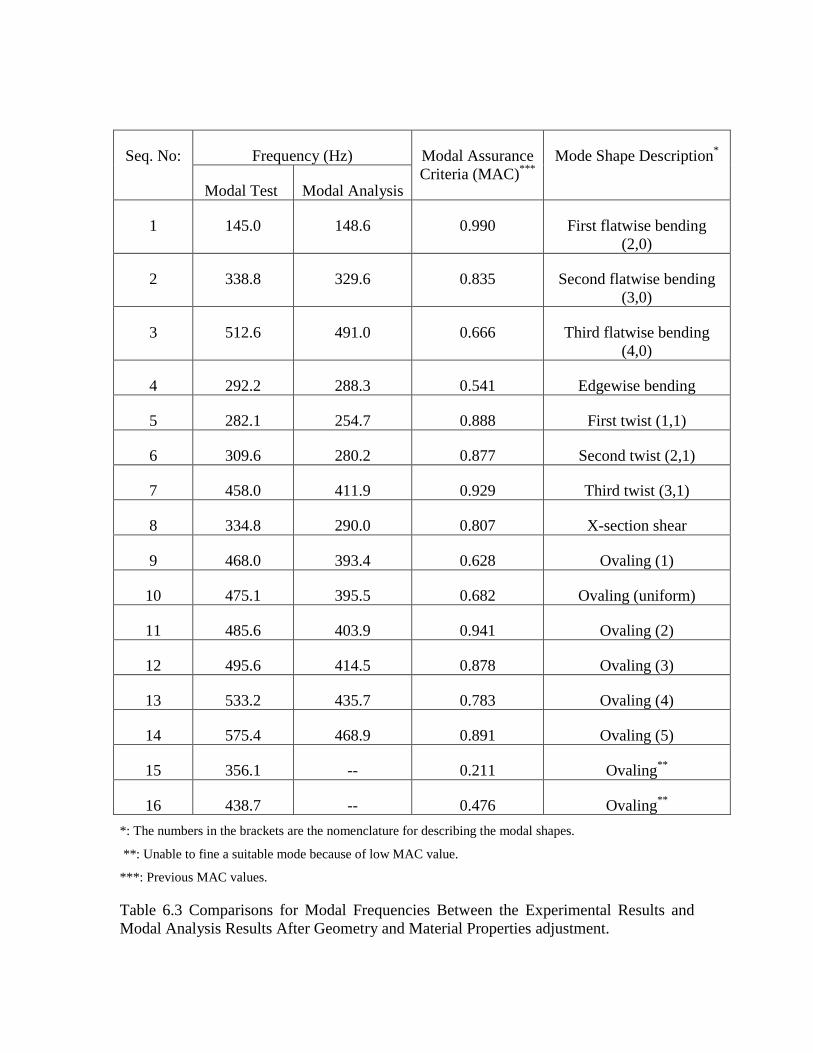
Frequency (Hz)Seq. No:

Modal Test Modal Analysis

Modal AssuranceCriteria (MAC)***

Mode Shape Description*

1 145.0 148.6 0.990 First flatwise bending(2,0)

2 338.8 329.6 0.835 Second flatwise bending(3,0)

3 512.6 491.0 0.666 Third flatwise bending(4,0)

4 292.2 288.3 0.541 Edgewise bending

5 282.1 254.7 0.888 First twist (1,1)

6 309.6 280.2 0.877 Second twist (2,1)

7 458.0 411.9 0.929 Third twist (3,1)

8 334.8 290.0 0.807 X-section shear

9 468.0 393.4 0.628 Ovaling (1)

10 475.1 395.5 0.682 Ovaling (uniform)

11 485.6 403.9 0.941 Ovaling (2)

12 495.6 414.5 0.878 Ovaling (3)

13 533.2 435.7 0.783 Ovaling (4)

14 575.4 468.9 0.891 Ovaling (5)

15 356.1 -- 0.211 Ovaling**

16 438.7 -- 0.476 Ovaling**

*: The numbers in the brackets are the nomenclature for describing the modal shapes.

**: Unable to fine a suitable mode because of low MAC value.

***: Previous MAC values.

Table 6.3 Comparisons for Modal Frequencies Between the Experimental Results andModal Analysis Results After Geometry and Material Properties adjustment.

Frequency (Hz)Seq. No:

Modal Test Modal Analysis

(Baseline)

Modal Analysis

(Final)

Mode Shape Description*

1 145.0 148.6 146.2 First flatwise bending(2,0)

2 338.8 329.6 330.3 Second flatwise bending(3,0)

3 512.6 491.0 496.1 Third flatwise bending(4,0)

4 292.2 288.3 281.3 Edgewise bending

5 282.1 254.7 264.6 First twist (1,1)

6 309.6 280.2 289.1 Second twist (2,1)

7 458.0 411.9 413.6 Third twist (3,1)

8 334.8 290.0 302.3 X-section shear

9 468.0 393.4 409.9 Ovaling (1)

10 475.1 395.5 412.2 Ovaling (uniform)

11 485.6 403.9 421.1 Ovaling (2)

12 495.6 414.5 431.4 Ovaling (3)

13 533.2 435.7 452.6 Ovaling (4)

14 575.4 468.9 485.5 Ovaling (5)

(a) 11.9 lb. 11.2 lb. 11.8 lb. D-spar Weight

(b) 0.147" 0.142" 0.148" Average Thickness*: The numbers in the brackets are the nomenclature for describing the modal shapes.

Table 6.4 Comparisons for Modal Frequencies Between the Experimental Results andModal Analysis Results After Fine Tuning.

Figure 6.1 Static Test Set-Up

P

�

�

x

y

x

y

z

Figure 6.2a Definition of Reference Axis

Kevlar String

W, (dead weight)

2.25 " y

z

Figure 6.2b Application of Load

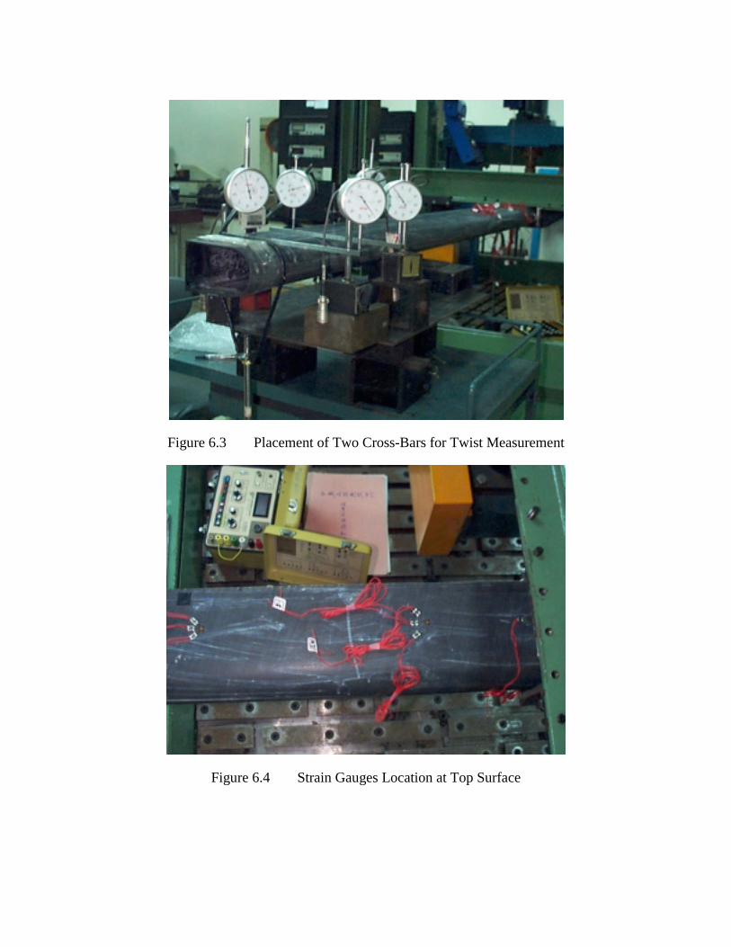
Figure 6.3 Placement of Two Cross-Bars for Twist Measurement

Figure 6.4 Strain Gauges Location at Top Surface

y = -0.0037xR2 = 0.9518

y = -0.0051xR2 = 0.9705

y = -0.006xR2 = 0.9925

-0.70

-0.60

-0.50

-0.40

-0.30

-0.20

-0.10

0.000 20 40 60 80 100 120

Weight (lb)

Def

lect

ion

(in)

x= 54" x= 66" x= 72" Linear (x= 54") Linear (x= 66") Linear (x= 72")

Figure 6.5 Vertical Deflection at the Measured Locations under Various Tip Loads

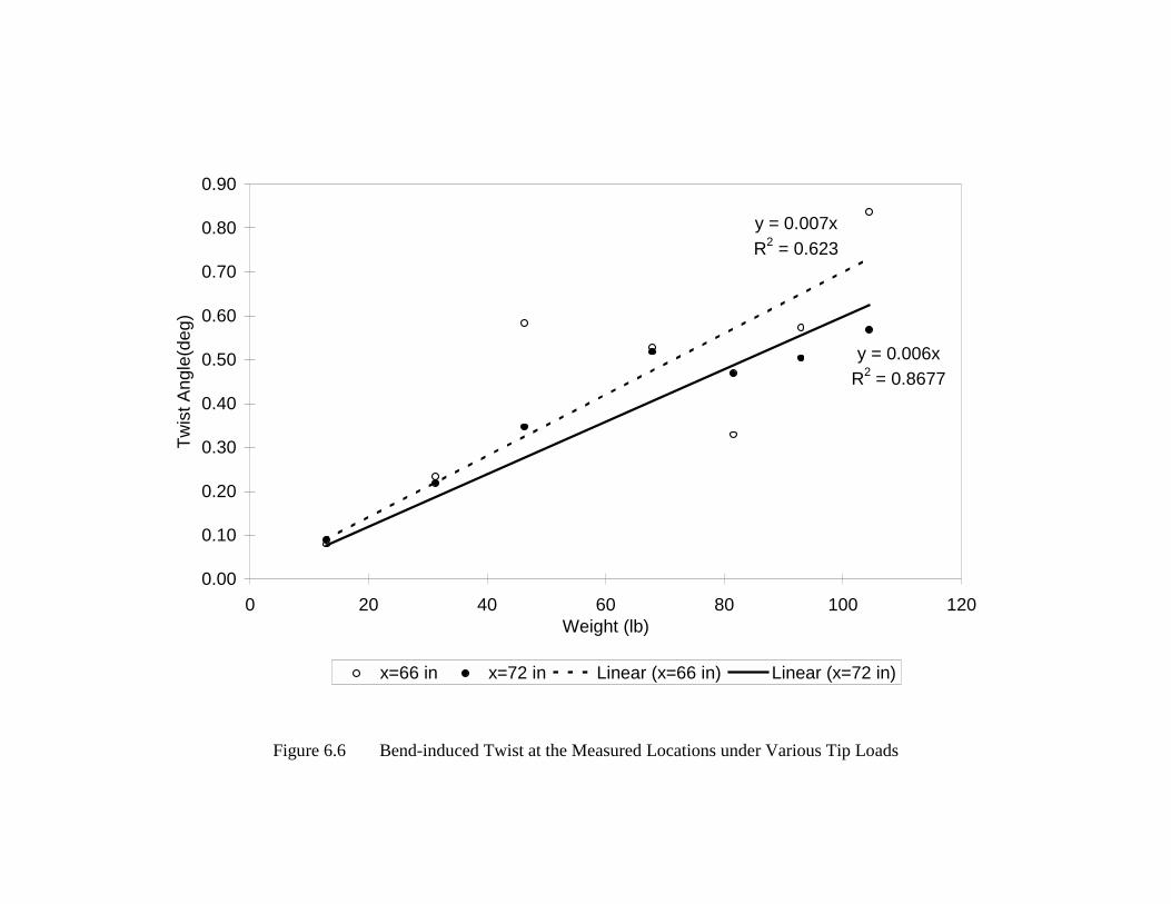
y = 0.007xR2 = 0.623

y = 0.006xR2 = 0.8677

0.00

0.10

0.20

0.30

0.40

0.50

0.60

0.70

0.80

0.90

0 20 40 60 80 100 120Weight (lb)

Twis

t Ang

le(d

eg)

x=66 in x=72 in Linear (x=66 in) Linear (x=72 in)

Figure 6.6 Bend-induced Twist at the Measured Locations under Various Tip Loads

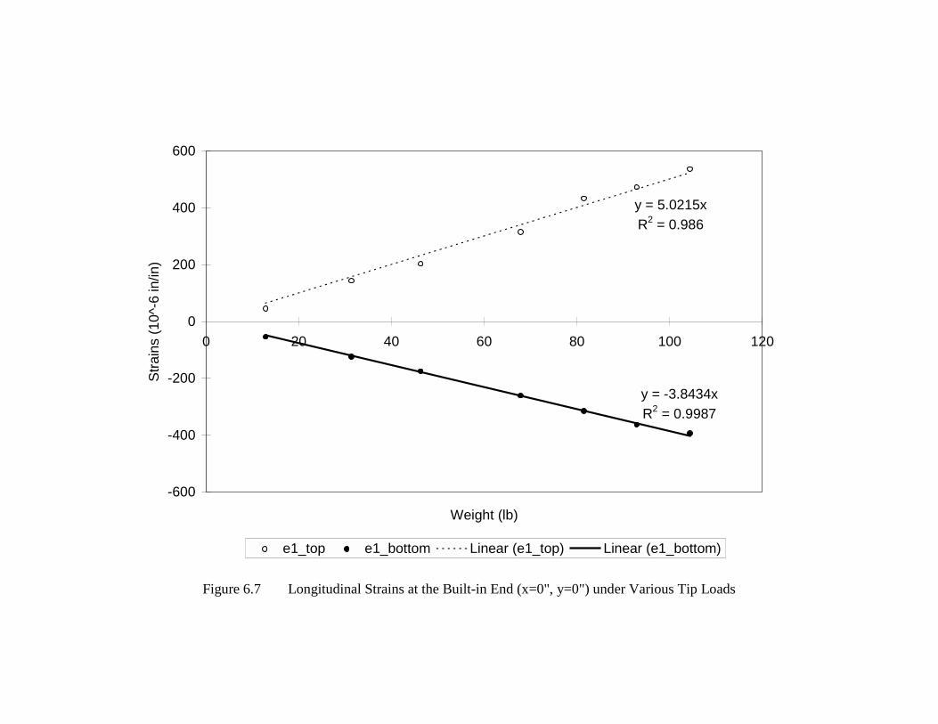
y = 5.0215xR2 = 0.986

y = -3.8434xR2 = 0.9987

-600

-400

-200

0

200

400

600

0 20 40 60 80 100 120

Weight (lb)

Stra

ins

(10^

-6 in

/in)

e1_top e1_bottom Linear (e1_top) Linear (e1_bottom)

Figure 6.7 Longitudinal Strains at the Built-in End (x=0", y=0") under Various Tip Loads

y = 4.6856xR2 = 0.9935

y = -2.7007xR2 = 0.9342

y = -6.8459xR2 = 0.9916

-800

-600

-400

-200

0

200

400

600

800

0 20 40 60 80 100 120

Weight (lb)

Stra

ins

(10^

-6 in

/in)

e1_top e2_top e6_top Linear (e1_top) Linear (e2_top) Linear (e6_top)

Figure 6.8a Strains at the Top Surface (x=6", y=0") under Various Tip Loads

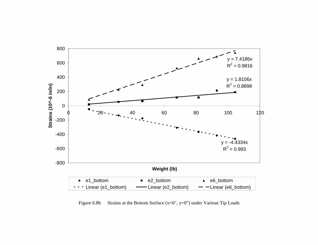
y = -4.4334xR2 = 0.993

y = 1.8106xR2 = 0.8898

y = 7.4186xR2 = 0.9816

-800

-600

-400

-200

0

200

400

600

800

0 20 40 60 80 100 120

Weight (lb)

Stra

ins

(10^

-6 in

/in)

e1_bottom e2_bottom e6_bottomLinear (e1_bottom) Linear (e2_bottom) Linear (e6_bottom)

Figure 6.8b Strains at the Bottom Surface (x=6", y=0") under Various Tip Loads

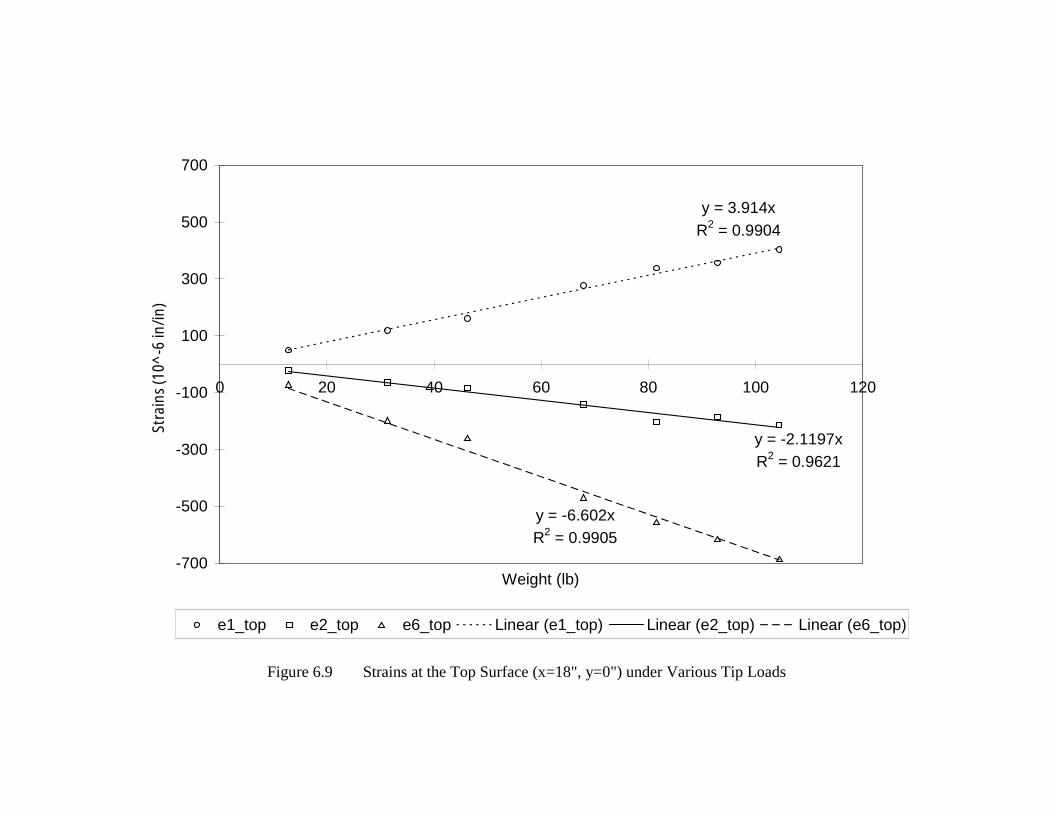
y = 3.914xR2 = 0.9904

y = -2.1197xR2 = 0.9621

y = -6.602xR2 = 0.9905

-700

-500

-300

-100

100

300

500

700

0 20 40 60 80 100 120

Weight (lb)

Stra

ins

(10^

-6 in

/in

)

e1_top e2_top e6_top Linear (e1_top) Linear (e2_top) Linear (e6_top)

Figure 6.9 Strains at the Top Surface (x=18", y=0") under Various Tip Loads

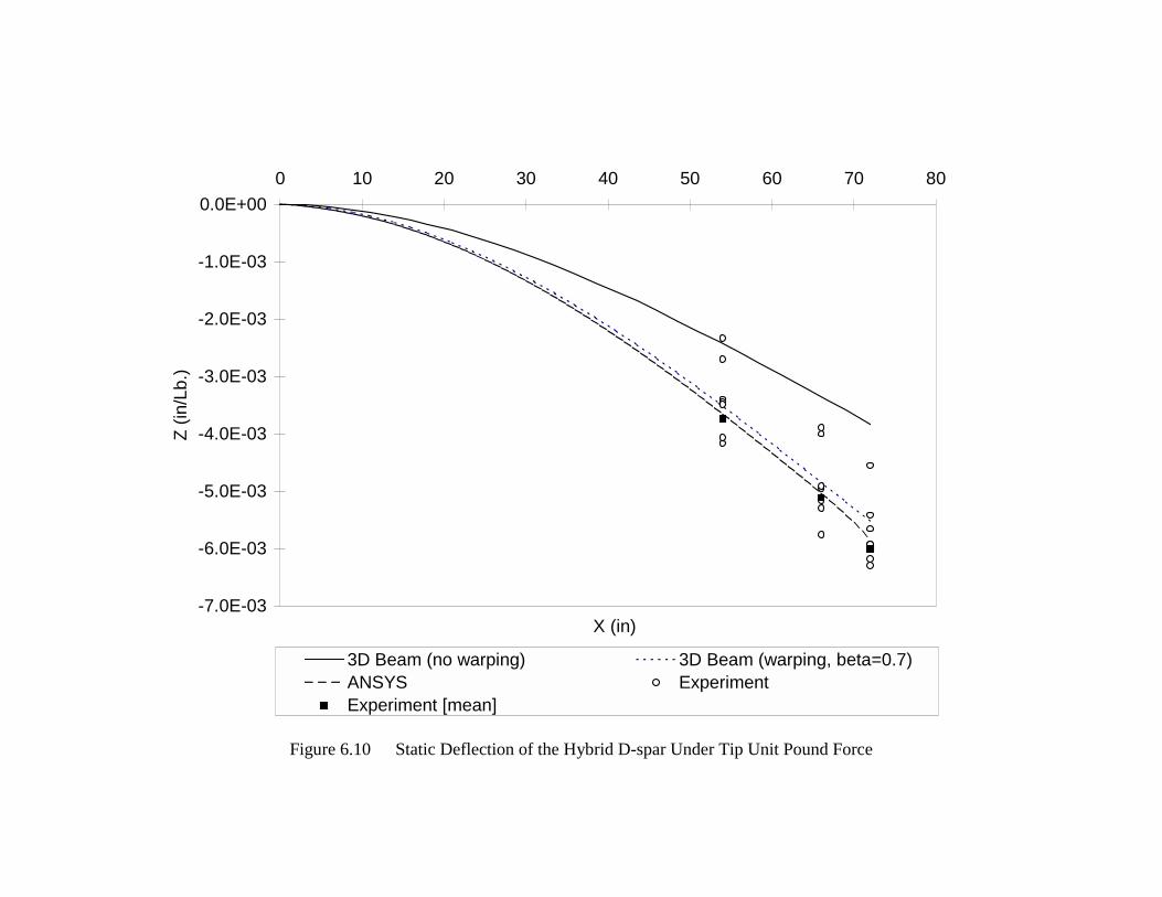
-7.0E-03

-6.0E-03

-5.0E-03

-4.0E-03

-3.0E-03

-2.0E-03

-1.0E-03

0.0E+000 10 20 30 40 50 60 70 80

X (in)

Z (in

/Lb.

)

3D Beam (no warping) 3D Beam (warping, beta=0.7)ANSYS ExperimentExperiment [mean]

Figure 6.10 Static Deflection of the Hybrid D-spar Under Tip Unit Pound Force

-2.0E-03

0.0E+00

2.0E-03

4.0E-03

6.0E-03

8.0E-03

1.0E-02

1.2E-02

1.4E-020 10 20 30 40 50 60 70 80

X (in)

Twis

t Ang

le (°

/Lb.

)

3D Beam (no warping) 3D Beam (warping, beta=0.7)ANSYS ExperimentExperiment (mean)

Figure 6.11 Bend-induced Twist of the Hybrid D-spar Under Tip Unit Pound Force

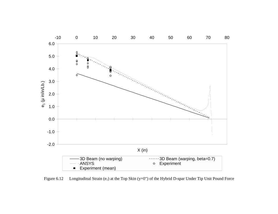
-2.0

-1.0

0.0

1.0

2.0

3.0

4.0

5.0

6.0-10 0 10 20 30 40 50 60 70 80

X (in)

e 1 (µ

in/in

/Lb.

)

3D Beam (no warping) 3D Beam (warping, beta=0.7)ANSYS ExperimentExperiment (mean)

Figure 6.12 Longitudinal Strain (e1) at the Top Skin (y=0") of the Hybrid D-spar Under Tip Unit Pound Force

-4.0

-3.0

-2.0

-1.0

0.0

1.0-10 0 10 20 30 40 50 60 70 80

X (in)

e 2 ( µ

in/in

/Lb.

)

3D Beam (no warping) 3D Beam (warping, beta=0.7)ANSYS ExperimentExperiment (mean)

Figure 6.13 Transverse Strain (e2) at the Top Skin (y=0") of the Hybrid D-spar Under Tip Unit Pound Force

-10.0

-8.0

-6.0

-4.0

-2.0

0.0

2.0-10 0 10 20 30 40 50 60 70 80

X (in)

e 6 ( µ

in/in

/Lb.

)

3D Beam (no warping) 3d Beam (warping, beta=0.7)ANSYS ExperimentExperiment (mean)

Figure 6.14 Shear Strain (e6) at the Top Skin (y=0") of the Hybrid D-spar Under Tip Unit Pound Force

Figure 6.15(a) First Flatwise Bending Mode (ANSYS; frequency= 146.2Hz)

Figure 6.15(b) First Flatwise Bending Mode (Modal Test; frequency= 145.0 Hz)

Figure 6.16(a) Second Flatwise Bending Mode (ANSYS; frequency= 330.3Hz)

Figure 6.16(b) Second Flatwise Bending Mode (Modal Test; frequency= 338.8Hz)

Figure 6.17(a) First Torsion Mode (ANSYS; frequency= 264.6Hz)

Figure 6.17(b) First Torsion Mode (Modal Test; frequency= 282.1Hz)

Figure 6.18(a) Second Torsion Mode (ANSYS; frequency= 289.1Hz)

Figure 6.18(b) Second Torsion Mode (Modal Test; frequency= 309.6Hz)

Chapter 7

Conclusions

The three key parameters that have the greatest effect on the coupling coefficientare the ply orientation, the laminate material, and the proportional volume of anisotropylayers in a laminate. A higher α value is achieved by having the ply orientation between15° and 30° and by using a high-performance ply material such as Graphite/Epoxy.Graphite/Epoxy D-spars have a maximum coupling around α=0.55, while those withGlass/Epoxy have a maximum coupling around α=0.4. The hybrid lay-up configurationhas an α close to that of the Graphite/Epoxy D-spar. Other parameters, such as thegeometry and the inclusion of internal rib, change the magnitude of α, but the effect isnot significant.

The three critical parameters have been fully utilized in the D-spar design. Toachieve the maximum tip rotation per unit pound force, the α value must be maximizedand the square root of the product of "EI" and "GJ" must be minimized. With using justone off-axis unidirectional lay-up, the desired structural properties were achieved towithin 15% for two of the three D-spar configurations.

Two D-spars, the all-carbon and the hybrid D-spars, were successfully fabricated.The staggered overlap joint that was invented during the fabrication eases the problemscaused by a butt joint or a single overlap joint design. The step-change in thicknesssurrounding the joint is drastically reduced with this new design. The cantilevered statictest demonstrated that the manufactured hybrid D-spar does produce the desired coupling.The test results generally indicate greater coupling than the numerical results (predictedby 3D-Beam) without torsion-related warping effect. When warping is included in thepredictions, much better agreement with test data is obtained, indicating a significantbeneficial effect on the bend-induced twist.

The predicted results of the ANSYS model (both static and modal analysis) areclose to the experimental results after the adjustments were made to better match the as-built D-spar geometry and material properties. Extensive study of parameter sensitivitywas not required because the baseline results are close to the modal test results. Minoradjustments on the modulus (Ex) and the thickness bring the average prediction error toless than 5% for the beam modes and torsion modes.

References

1. T. Weisshaar, "Aeroelastic Tailoring - Creative Uses of Unusual Materials," AIAAPaper No. 87-0976-CP, 1987.

2. E. C. Smith and I. Chopra, "Formulation and Evaluation of an Analytical Model forComposite Box-Beams," AIAA-90-0962-CP, 1990.

3. Ramesh Chandra, Alan D. Stemple, and Inderjit Chopra, “Thin-Walled CompositeBeams Under Bending, Torsional, and Extensional Loads,” Journal of Aircraft, Vol.27, No. 7, July 1990.

4. N.M. Karaolis, P.J. Mussgrove and G. Jeronimidis, "Active and Passive AerodynamicPower Control Using Asymmetric Fiber Reinforced Laminates for Wind TurbineBlades," Proc. 10th British Wind Energy Conf., D.J. Milbrow Ed., London, March 22-24, 1988.

5. N.M. Karaolis, G. Jeronimidis and P.J. Mussgrove, "Composite Wind TurbineBlades: Coupling Effects and Rotor Aerodynamic Performance," Proc., EWEC'89,European Wing Energy Conf., Glasgow, Scotland, 1989.

6. H.J.T. Koijman, "Bending-Torsion Coupling of a Wind Turbine Rotor Blade," ECN-I-96-060, December 1996.

7. D.W. Lobitz, P.S. Veers and P.G. Migliore, "Enhanced Performance of HAWTsUsing Adaptive Blades," Proc. Wind Energy '96, ASME Wing Energy Symposium,Houston, Jan. 29 - Feb. 2, 1996.

8. D.W. Lobitz and D.J. Laino, "Load Mitigation with Twist-Coupled HAWT Blades,"Proceedings of the 1999 ASME Wing Energy Symposium, Reno, January 11-14, 1999.

9. D.W. Lobitz and P.S. Veers, "Aeroelastic Behavior of Twist-Coupled HAWTBlades," AIAA-98-0029, Proc. 1998 ASME Wind Energy Symposium held at 36th

AIAA Aerospace Sciences Meeting and Exhibition, Reno, NV, Jan. 12-15, 1998.

10. S. Shinh, "Composite Blade Model and Software," XAF-4-14076-01, September1997.

11. C.H. Ong., "Composite Tubular Structures," Proceedings of the Fifth JapanInternational SAMPE Symposium, October 38-31, 1997

12. S.W. Tsai and H. T. Hahn, Introduction to Composite Materials, TechnomicPublishing Company, Inc., 1980.

13. T.G. Carne and B.D. Boughton, "Modal Testing of the Graphite and Hybrid D-Sparsfor Model Validation," Internal Memorandum, Sandia National Laboratories, March25, 1999.