Design fine tuning using MATLAB and SIMULINK for flow ... · PDF fileTitle Design fine tuning using MATLAB and SIMULINK for flow control devices Authors: Ramakumar Methrukovil Pradeep

Title

Design fine tuning using MATLAB and

SIMULINK for flow control devices

Authors:

Ramakumar Methrukovil

Pradeep Bhagavath

Thara Manohar

WHITE PAPER Design fine tuning using MATLAB and SIMULINK

Wipro Technologies Page 2 of 25

Abstract

Linear Drive System is a fluid control device used to control the suction volume of the fluid drained from human body during Endoscope surgery. The product comprises of Disposable cassette, Drive mechanism and power supply used in conjunction with Endoscope and Suction source.

Different types of the fluids like water, urografin, gas mixed liquids, gases and waste fluids are required to be drained during endoscope surgery. Controlled outflow rate of the fluid depends on many parameters like pressure, temperature, viscosity, pipe length, type of valve, fluid parameters, etc.

In this white paper, for better understanding, entire system is divided in to four parts: motor, drive unit, valve and pipe flow. Only water properties are considered for the calculation. Since the system requirement is linear relationship between flow rate and valve position, linear stepper motor is a preferred choice. So suitable stepper motor can be selected after calculating maximum force required to close the valve completely.

Drive unit will convert step position i.e. input knob position in to linear travel of stepper motor. Drive hardware and motor driver circuit will control the accurate movement of the motor.

Valve or disposable cassette is a heart of this system through which controlled outflow is achieved. Different innovative valve concepts can be developed based on the flow requirement but flow calculation procedure will remain almost same for any of the concepts. In this white paper flow calculation and behavior is studied only for diaphragm type cassette or valve.

As flow rate depends on many variable parameters, it is necessary to check the system behavior with different variables. So mathematical relationship is derived between flow rate and other dependent parameters on the basis of fluid dynamics theory.

These derived relationships are used in MATLAB to study the system behavior graphically. MATLAB results are used for fine tuning many design parameters like: optimum diameter of the diaphragm for complete valve closing, selection of stepper motor for maximum force requirement, fixing the pipe length to achieve required flow rate, fine tuning the flow rate vs. linear travel relationship for different pressure and temperatures.

Similarly SIMULINK model is designed for entire system. For ease of usage, model is divided into main and sub-system. In the main system suction pressure, temperature, pipe length and step position are inputs. Based on these input values, fluid calculation is done in subsystem and suitable output is displayed.



Table of Contents

1 INTRODUCTION ................................................................................................................ 4 2 LINEAR DRIVE SYSTEM (LDS) ........................................................................................ 4 3 REQUIREMENTS AND SPECIFICATION ......................................................................... 5 4 METHODOLOGY ............................................................................................................... 6

4.1 Motor ........................................................................................................................... 6 4.2 Linear Drive Unit ......................................................................................................... 6 4.3 Valve ........................................................................................................................... 6 4.4 Flow Rate: ................................................................................................................. 10

5 CONCLUSION ................................................................................................................. 23

Figures

Figure 1: System Configuration ................................................................................................. 4 Figure 2: Input-Output relationship of different blocks............................................................... 6 Figure 3 : Diaphragm Concept Figure 4 : Deformed shape of the diaphragm ......................... 7 Figure 6 : Displacement and stress vs. r/h ratio ........................................................................ 8 Figure 7 : Relationship force vs. linear travel of LDU ................................................................ 9 Figure 8 : Concept of entrance length ..................................................................................... 10 Figure 9 : Moody Chart ............................................................................................................ 11 Figure 12 : AEB-Effective area after deformation .................................................................... 13 Figure 13 : Inflow rate vs. pipe length for water at 0.50kPa pressure ..................................... 16 Figure 14 : Inflow rate vs. pipe length for water at 26.7kPa pressure ..................................... 16 Figure 15 : Inflow rate vs. pipe length for water at 50kPa pressure ........................................ 17 Figure 16 : Inflow rate vs. pipe length for water at 100kPa pressure ...................................... 17 Figure 17 : Outflow rate vs. linear travel of LDU for water at 0.5kPa pressure ....................... 18 Figure 18 : Outflow rate vs. linear travel of LDU for water at 26.7kPa pressure ..................... 18 Figure 19 : Outflow rate vs. linear travel of LDU for water at 50kPa pressure ........................ 19 Figure 20 : Outflow rate vs. linear travel of LDU for water at 100kPa pressure ...................... 19



1 INTRODUCTION

Flow is a general term has different meaning in different context. According to Fluid mechanics flow is nothing but fluids in motion and theory which deals with it is called as Fluid Dynamics. There are many types of flow control devices available in medical industry. Applications of these devices are for controlled drug delivery, draining of waste fluid from the body, Respiratory control and so on. Rate of flow of fluid through these devices depends on many parameters like Pressure, Area of cross section, Density and Viscosity of fluid, Temperature variation, friction losses and length of the pipe.

This white paper describes the behavior of flow control device, used during endoscope surgery, for variation of different parameters. This flow control device is called as linear drive system used for draining waste fluid from body during endoscope operation. Most flexible and user friendly nature of MATLAB and SIMULINK software helps in understanding relationship of flow rate with various other parameters.

2 LINEAR DRIVE SYSTEM (LDS)

The system configuration consisting of linear drive unit (LDU) is intended to use along with endoscope and suction pump for fluid flow control from endoscope.

The product features of linear drive system are:

Product has three subsystems

Linear drive unit

Disposable Cassette and

Power unit

The LDU consists of drive and controlling hardware.

The power unit consists of power supply and user interface for Linear Drive Unit.

The suction end of cassette shall be connected to Endoscope and the discharge end to the suction pump.

The fluid flow through the cassette shall be controlled using a Rotary knob in 60 steps.

This system will be used along with disposable cassette designed for fluid flow control from Endoscope and also with any other cassettes designed in future.

Figure 1: System Configuration



3 REQUIREMENTS AND SPECIFICATION Following are the major requirements of the flow control device.

Target fluid:

High viscous fluids - Egg white, Urografin 76%

Low viscous fluids- Water, gas mixed liquid

Maximum fluid flow: 630 ~ 730 ml/min @ suction pressure of 26.7kPa

Suction Pressure: Varies from 0-100KPa

Flow control gradient count: 60 steps

ON and OFF Response Time: Target for Water Response time is 150ms or less

The maximum linear action shall be 10mm

The set stroke distance shall be within +/-0.01 mm accuracy

Speed of movement: Not less than five round/trip per second

Tube diameter: 4.0mm ID

Working temperature : 10 – 40 Deg C

Following material specifications are considered for Analysis.

Modulus of elasticity of silicon rubber: 90x106 Pa

Poisson‟s Ratio of silicon rubber : 0.3

Internal Fluid pressure:26.7 KPa

Thickness of the diaphragm : 0.40mm

Operating Voltage : 12V

Stepper motor coil Resistance : 84 Ohms

Stepper motor coil Inductance : 33.6 mH



4 METHODOLOGY

For mathematical modeling the entire system is divided in to four blocks namely:

Motor Linear Drive Unit Valve Flow rate

Figure 2: Input-Output relationship of different blocks

4.1 Motor

To achieve linear relationship between outflow rate and displacement, linear stepper motor will be used to drive the system. Schematically linear stepper motor consists of Resistance and Inductor connected in series to DC source. According to Kirchhoff‟s voltage law, Voltage

…… (1) Above equation can be written as:

…… (2)

Where XL is the inductive reactance given by XL = 2∏fL therefore inductor offers resistance to DC source, and equation (1) reduces to V = IR. Power required to drive is given by,

…… (3) By substituting values of Voltage and current, we can find out the power required to drive the system.

4.2 Linear Drive Unit As per the functional requirement, flow control gradient count= 60 steps. That means the LDU has to complete its movement in 60 steps. In the present problem the linear drive unit has to move „d‟ mm in 60 steps, therefore linear travel per step is d/60. If n is number of cycles per second then number of steps/sec = 60n. Since in this case it has to complete one cycle in second, n=1.Linear travel per second is given by number of steps per second times linear travel per step.

4.3 Valve Many valve concepts are developed to meet flow rate requirement. Only diaphragm concept is discussed in this white paper. In this concept as linear drive unit moves by a distance δ it applies a displacement boundary condition on the diaphragm and thus displacement of diaphragm is equal to linear travel of LDU.



Figure 3 : Diaphragm Concept Figure 4 : Deformed shape of the diaphragm

Calculation of radius and thickness of the diaphragm:

Static displacement of diaphragm is obtained by considering it as a circular plate constrained from all the edges subjected to a uniform pressure as shown in the below sketch.

According to plate theory, formula for deflection of the diaphragm is given by,

……. (4)

Where „a‟ varies from 0 to r. Maximum deflection occurs at the center of the diaphragm when a=0. And effective pressure P=Pext-Pin

D is effective flexural rigidity given by,

…… (5)

So maximum deflection at the center is given by,

Figure 5 : Uniform load on the diaphragm



…… (6)

And stress induced in the diaphragm is given by,

…… (7)

From maximum deflection formula (6), it can be derived that net pressure exerted on the diaphragm P is equal to 10Kpa when suction pressure is set at 26.7kPa.

So external pressure on the diaphragm is Pext=Pin + P = 36.7KPa.

From the above two equations (6) and (7), graph of deflection and stress with respect to r/h ratio can be plotted, as shown below.

Figure 6 : Displacement and stress vs. r/h ratio

Form the graph; to close the 4.0mm diameter pipe (i.e. for 4.0mm deflection) r/h ratio should be 28 which correspond to a stress of 6MPa which is well below its ultimate strength of silicone rubber. Considering manufacturing point of view thickness of the diaphragm is fixed to 0.40mm. So r=28*0.40=11.20mm

MATLAB Code:

% Matlab code for r/h ratio calculation clear all clc E=90e6;% Modulus of Elasticity of Silicone Rubber Membrane in Pa r=linspace(0.1e-3,20e-3,1000); % Radius of the diaphragm, range from 0.1 to 20mm h=0.4e-3; % Thickness of the diaphragm, assumed nu=0.48; % Poisson's Ratio for Silicone rubber D=E*h^3/(12*(1-nu^2)); % Flexural Rigidity q=10e3; % Effective pressure delta=q.*(r.^2).^2./(64*D); %Deflection of the diaphragm sigma=3*q.*r.^2./(4*h^2); % Stress induced in the diaphragm plot(r./h,delta*1e3,r./h,sigma*1e-6,'--'); grid



Calculation of force required to compress the diaphragm:

Force required from the linear motor to have δ mm displacement of diaphragm is given by,

F=Pext*A…. (8)

Where „Pext‟ is external pressure required to have δ mm displacement of diaphragm and it varies depends on internal pressure of fluid. „A‟ is area of diaphragm=∏r2.

Figure 7 : Relationship force vs. linear travel of LDU

MATLAB Code:

% Matlab code shows relation between Drive force and linear travel of LDU % for DIAPHRAGM CONCEPT clear all; clc; E=90e6; % Modulus of Elasticity of Silicone Rubber Membrane in Pa r=11.2e-3; % Radius of the diaphragm in mtrs h=0.4e-3; % Thickness of the diaphragm in mtrs nu=0.48; % Poisson's Ratio for Silicone Rubber Pin=26.7e3; % Suction Pressure varies from 0.5KPa to 100Kpa D=E*h^3/(12*(1-nu^2)); % Flexural Rigidity Delta=linspace(0,4e-3,100); % Required deflection of the diaphragm in mtrs P=64*D*Delta/r^4; %Net Pressure acting on the diaphragm in Pa Pt=Pin+P; %External pressure acting on the diaphragm in Pa F=Pt*pi*r^2; % Force acting on the diaphragm in newton plot(Delta,F); % Graph of force vs deflection grid xlabel('Linear Travel of LDU in m') ylabel('Froce Required from Linear Motor in Newton')

So from the graph it can be concluded that selected stepper motor should exert at least 44N force to work under suction pressure of 100KPa.



4.4 Flow Rate:

Flow in a pipeline can be classified into laminar, turbulent or transition regime based on the value of Reynolds number which is the ratio of inertial forces to viscous force given by expression,

…… (9)

Where ρ is the density of fluid, v is velocity of the fluid particle, d is diameter of pipe and µ is dynamic viscosity of the fluid. If “Q” is the flow rate at inlet section then using continuity equation Q = av we get the velocity. Depending upon the value of Reynolds number we classify the flow regime and suitable formulations are used.

Any fluid flowing in a pipe has to enter the pipe at some location. The region of flow near where the fluid enters the pipe is termed as entrance region and is illustrated in figure 8. Here entrance region is from patient body to endoscope.

Figure 8 : Concept of entrance length

As shown in figure 8, the fluid typically enters the pipe with nearly uniform velocity profile at the entrance. As the fluid moves through the pipe, viscous effects cause to stick to the pipe wall. At a finite distance from the entrance, the boundary layers merge and inviscid core disappears. The tube flow is the entirely viscous, and axial velocity adjust slightly further until at x=Le, it no longer changes with x and said to be fully developed. The boundary layer has grown in thickness to completely fill the pipe. Viscous effects are of considerable importance within the boundary layer. For fluid outside the boundary layer viscous effects are negligible.

The shape of velocity profile in the pipe depends on whether the flow is laminar or turbulent, as does the length of entrance region, Le. As with many other pipe flow, the dimensionless entrance length, correlates quite well with the Reynolds number. Typical lengths are given by,

…… (10)

…… (11)



Calculation of velocity and pressure distribution within the entrance region is quite complex. However, once the fluid reaches the end of entrance region, the flow is simpler to describe because velocity is function of only distance from the pipe centerline, r, and independent of x this is termed as fully developed flow. So in this scenario, it is necessary to calculate the length of the pipe required to achieve required flow rate and has to see whether flow is in entrance region or is in fully developed region. Head loss due to friction:

Using Darcy weisbach formula we have head loss due to friction as:

….... (12) Where „f‟ is a constant depends upon the value of Reynolds number known as friction factor. Assuming smooth pipe, close expression for calculation of „f‟ for laminar flow is given by,

…… (13)

And that for turbulent flow is given by moody chart as shown in figure 9. The closed form expression for friction factor in smooth pipes with turbulent flow is given by,

…… (14)

Figure 9 : Moody Chart

Minor Losses:

For any pipe system in addition to Moody-type friction loss computed for the length of pipe, there are additional so-called minor losses due to

a) Pipe entrance or exit.

b) Sudden expansion or contraction.

c) Bends, elbows, tees, and other fittings.

d) Valves, open or partially closed.

e) Gradual expansion or contractions.



The losses may not be so minor, e.g.: a partially closed valve can cause a greater pressure drop than long pipe. Since the flow pattern in fittings and valves is quite complex, the theory is very week. The losses are commonly measured experimentally and correlated with the pipe flow parameters. The data, especially for valves are somewhat dependent upon the particular manufacturer's design, so that the values listed there must be taken as average design estimates. The measured minor losses are usually given as a ratio of the head loss, hm=∆P / (ρg), through the device to the velocity head v2/ (2g) of the associated pipe system

…… (15)

A single pipe system may have many minor losses. Since all are correlated with v2/ (2g) they can be summed into a single total system loss if the pipe has constant diameter

….. (16) There are many different valve designs in commercial use. Figure 10 shows the gate valve, which slides down across the section. Figure 11 shows the variation of loss coefficient as a function of fractional opening. It can be seen that as the fractional opening reduces the loss coefficient shoots up thus minor losses play an important role when the fractional opening is very small.

Inflow Rate:

It can be seen from figure 10 that, when the valve is completely open minor loss coefficient, K = 0, therefore the loss is only due to friction, and equation (16) reduces to:

…….. (17) ** The curve shown is experimental that accounts for generalized shape variations. For more exact solutions, either experiments have to be done or a CFD simulation of that region is required.

As per the requirement for flow rate is 700 ml/min at a suction pressure of 26.7KPa, Flow will be in turbulent region. So for turbulent flow, using equation (14) we get, total head loss to be:

Figure 11 : Gate Valve Figure 10 : Minor loss coefficient for different valve

openings



…….. (18) Writing Reynolds number in terms of density and viscosity of fluid equation (19) reduces to:

…… (19) Applying continuity equation and expressing equation (19) in terms of pressure we get inflow rate as,

…….. (20)

Outflow Rate:

From equation (16) we have total pressure head as

……. (21) From figure 11 Friction loss coefficient, K depends upon the valve type and displacement of LDU. Making a polynomial fit with the data provided in figure 10 we get:

….. (22)

Where x=h/d.

Equation (21) can be written as:

……. (23) From equation (23) outflow can be expressed as:

….. (24) Where a‟ is the cross-sectional area of the pipe after deformation. After deflection of diaphragm by δ mm area of segment of pipe is ABE (Ref. Figure 12)

…… (25)

Figure 12 : AEB-Effective area after deformation



If θ is the angle between OA and OB then area of the segment ABD is given by,

…… (26) From right angled triangle OAC we have,

…… (27) And the effective area, a‟ is given by,

……. (28) Variation of viscosity with respect to change in temperature:

Temperature variation has a strong effect when compared to the pressure variation on viscosity. Liquid viscosity decreases with increase in temperature. From the experimental results relation between viscosity and temperature for the liquids can be arrived as,

……. (29) Where µ0 is the viscosity at given standard temperature T0.

For water,

T0 = 273.16K,

µ0 = 0.001792 Kg/m.s.

a = -1.94,

b = -4.80,

c = 6.74.

µ is the calculated viscosity for a given temperature T.

The error of calculated value of viscosity will be with in +/- 1 percent.

To calculate viscosity variation with respect to temperature for other liquids, we should know value of a, b and c.

MATLAB Code Inflow rate vs. pipe length for water: % Matlab Code shows relation between Inflow rate and pipe length for WATER % for DIAPHRAGM CONCEPT clear all clc P=26.7e3; %Suction Pressure in Pa, varies from 0.5KPa to 100KPa d=4e-3; % Diameter of the pipe in mtrs. Assumed constant throughout a1=pi.*d.^2./4; % Area of cross section of the pipe mue0=1.7922e-3; % Viscosity of water at 0 Deg C Tk0=273.16; % 0 Deg temperature in Kelvin Tk=273.16+20; % Water temperature in Kelvin y=-1.94-4.80.*(Tk0./Tk)+6.74.*(Tk0./Tk).^2; mue=mue0*exp(y); % Viscosity at given temperature Tk rho=1000; % Density of water in Kg/m3 l=linspace(50e-3,6,1000); % Length of the pipe varies from 50mm to 10mtrs num=P.*d^(5/4); den=0.158*rho^(3/4)*mue^(1/4).*l; Q=a1.*(num./den).^(4/7); % Inflow rate to the cassette in m3/s plot(l,Q*60e6) % Pipe length 'mtrs' vs Inflow rate 'ml/min' grid xlabel('Length of the pipe in m') ylabel('Inflow rate in ml/min')



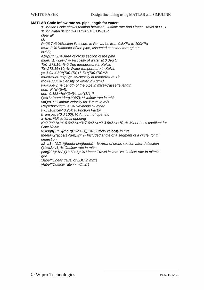
MATLAB Code Inflow rate vs. pipe length for water: % Matlab Code shows relation between Outflow rate and Linear Travel of LDU % for Water % for DIAPHRAGM CONCEPT clear all clc P=26.7e3;%Suction Pressure in Pa, varies from 0.5KPa to 100KPa d=4e-3;% Diameter of the pipe, assumed constant throughout r=d./2; a1=pi.*r.^2;% Area of cross section of the pipe mue0=1.792e-3;% Viscosity of water at 0 deg C Tk0=273.16; % 0 Deg temperature in Kelvin Tk=273.16+10; % Water temperature in Kelvin y=-1.94-4.80*(Tk0./Tk)+6.74*(Tk0./Tk).^2; mue=mue0*exp(y); %Viscosity at temperature Tk rho=1000; % Density of water in Kg/m3 l=6+50e-3; % Length of the pipe in mtrs+Cassette length num=P.*d^(5/4); den=0.158*rho^(3/4)*mue^(1/4)*l; Q=a1.*(num./den).^(4/7); % Inflow rate in m3/s v=Q/a1; % Inflow Velocity for 'l' mtrs in m/s Rey=rho*v*d/mue; % Reynolds Number f=0.316/(Rey^0.25); % Friction Factor h=linspace(0,d,100); % Amount of opening x=h./d; %Fractional opening K=2.2e2.*x.^4-6.6e2.*x.^3+7.6e2.*x.^2-3.9e2.*x+70; % Minor Loss coeffient for Gate Valve v1=sqrt(2*P./(rho.*(f.*l/d+K))); % Outflow velocity in m/s theeta=2*acos(1-(d-h)./r); % Included angle of a segment of a circle, for 'h' deflection a2=a1-r.^2/2.*(theeta-sin(theeta)); % Area of cross section after deflection Q1=a2.*v1; % Outflow rate in m3/s plot((d-h)*1e3,Q1*60e6); % Linear Travel in 'mm' vs Outflow rate in ml/min grid xlabel('Linear travel of LDU in mm') ylabel('Outflow rate in ml/min')



Graphs of Inflow rate vs. length of the Pipe for Water for different Pressures:

Figure 13 : Inflow rate vs. pipe length for water at 0.50kPa pressure

Figure 14 : Inflow rate vs. pipe length for water at 26.7kPa pressure



Figure 15 : Inflow rate vs. pipe length for water at 50kPa pressure

Figure 16 : Inflow rate vs. pipe length for water at 100kPa pressure



Graphs of Outflow rate vs. linear travel of LDU for Water for different Pressures: (Pipe length of 6m is considered)

Figure 17 : Outflow rate vs. linear travel of LDU for water at 0.5kPa pressure

Figure 18 : Outflow rate vs. linear travel of LDU for water at 26.7kPa pressure



Figure 19 : Outflow rate vs. linear travel of LDU for water at 50kPa pressure

Figure 20 : Outflow rate vs. linear travel of LDU for water at 100kPa pressure



SIMULINK Models: SIMULINK models are designed based on the derived mathematical equation. In the main system suction pressure, temperature, pipe length and step position are inputs. Based on these input values, fluid calculation is done in subsystem and suitable output is displayed.

A. Main System

B. Viscosity Model



C. Inflow Rate:



D. Outflow Rate:



5 CONCLUSION

1. Inflow rate

From the derived equation (20) it can be concluded that inflow rate is directly proportional to the suction pressure, pipe diameter and inversely proportional to the density, viscosity and pipe length. Viscosity in turns depends on liquid temperature. From the graphs of Inflow rate vs. pipe length plotted using MATLAB, we can say that, as temperature increases, for set pressure, pipe length also increases to achieve required flow rate. But practically it is not possible to vary pipe length every time as fluid and its temperature changes, to achieve required inflow rate. So if pipe length is kept constant then variable is only suction pressure. From the plotted graphs, we can calculate that inflow rate increase by 10.5% for given pipe length, as the temperature varies from 10 to 40 deg C for any set pressure.

2. Outflow rate

From the derived equation (24) it can be concluded that outflow rate is directly proportional to the suction pressure and effective area of pipe and inversely proportional to the density, friction factor, pipe length and minor loss coefficient. Effective area of pipe after deflection of δ mm is calculated theoretically. Graphs of outflow rate vs. linear travel are plotted considering 6mtrs pipe length. From the graphs we can see variation of outflow rate as fluid temperature changes. Major conclusion from the graph is that out flow vs. linear travel relation is not exactly linear. It starts with zero slopes in the beginning, and then become nearly linear in the middle region and ends again with zero slopes.

3. Drive Force

From the graph of force vs. linear travel (figure-7), it can be concluded that selected stepper motor should exert at least 44N force to work under maximum suction pressure of 100KPa.

4. Usage of MATLAB and SIMULINK

As shown in the beginning of this paper, MATLAB software is effectively used to find out best suitable diameter of the diaphragm, which is a core part of the valve, for maximum deflection value. By using this software we could able to see the behavior of inflow rate vs. pipe length as the temperature and suction pressure of the system changes. Also using MATLAB software helped in finding out exact relationship between outflow rate and linear travel of LDU at different temperature and pressures. We can conclude by saying that it is not possible to get exact linear relationship between outflow rate and linear travel for this type of valve concept.



References

1. Fluid Mechanics by Frank M White, Sixth edition, TATA McGraw - Hill Publication.

2. Fluid Mechanics by Yunus A. Cengel and John M. Cimbala, 2006 edition, TATA McGraw - Hill Publication.

3. Getting Started with MATLAB 7 by Professor Rudra Pratap, Oxford University press Publication.

4. A guide to MATLAB by Brian R. Hunt, Ronald L. Lipsman and Jonathan M. Rosenberg, Cambridge University press publication.

About the Authors

Ramakumar is a Bachelor in Mechanical Engineering having around 16 years experience different functions like Quality assurance and Product development for multiple domains, e.g. Medical, Telecom etc.. Presently he is working as Project manager in Engineering Design services for Wipro Technologies.

Pradeep is a Bachelor in Mechanical Engineering having around 7 years experience in design and development of variety of products for different domains like Auto-electrical, Electro-mechanical, Connectors and Medical. Presently he is working as senior project engineer in Engineering Design services for Wipro Technologies.

Thara Manohar is a Diploma engineer in Mechanical Engineering having around 13 years experience in design and development and manufacturing area of variety of products for different domains like Industrial components, Electro-mechanical, and Medical domain. Presently he is working as senior project engineer in Engineering Design services for Wipro Technologies.



About Wipro Technologies

Wipro is the first PCMM Level 5 and SEI CMMi Level 5 certified R & D, IT and Enterprise Services Company globally. Wipro provides comprehensive IT solutions and services (including systems integration, IS outsourcing, package implementation, software application development and maintenance) and Research & Development services (hardware and software design, development and implementation) to corporations globally. Wipro's unique value proposition is further delivered through our pioneering Offshore Outsourcing Model and stringent Quality Processes of SEI and Six Sigma.

© Copyright 2002. Wipro Technologies. All rights reserved. No part of this document may be reproduced, stored

in a retrieval system, transmitted in any form or by any means, electronic, mechanical, photocopying, recording, or

otherwise, without express written permission from Wipro Technologies. Specifications subject to change without

notice. All other trademarks mentioned herein are the property of their respective owners. Specifications subject to

change without notice.

Documents

Design fine tuning using MATLAB and SIMULINK for flow ... · PDF fileTitle Design fine tuning using MATLAB and SIMULINK for flow control devices Authors: Ramakumar Methrukovil Pradeep