Embed Size (px)
Citation preview

DIPLOMA THESIS
DESIGN DEVELOPMENT AND
PRODUCTION OF
ELECTROMAGNETIC COILS FOR
ATTITUDE CONTROL OF
A PICO SATELLITE
Ali Aydinlioglu
Matr. Nr. 183875
Supervisors:
Prof. Dr.-Ing. W. Ley
Prof. Dr.-Ing. G. Schmitz
Dipl.-Ing. Jens Gieselmann
Aachen, February 2006

II
I assure that I have composed the thesis autonomously with a support of the group and
that I have only used references as mentioned. References are marked in the report and
listed in a table.
This thesis is prepared to the best of my knowledge.
Aachen, February 2006
Ali Aydinlioglu


Abstract
IV
Abstract
The Compass-1 CubeSat is an actively controlled picosatellite utilizing magnetic coils
as only means of attitude control. The Attitude Determination and Control System
(ADCS) provides the three-axis stabilizing capability. The ADCS was developed to
stabilize the spacecraft against disturbances resulting from the spacecraft LEO
environment. Magnetic coils are strapped to the satellite structure to generate the control
torques.
This thesis presents the study carried out to establish three identical magnetorquer for an
actively controlled picosatellite.
The design and development of the magnetorquer as well as the essential hardware for
producing the magnetorquer, the coil winder, is elaborated.
Keywords
CubeSat, picosatellite, Compass-1, ADCS Attitude Determination and Control System,
three- axis stabilizing, magnetorquer

Acknowledgements
V
Acknowledgements
I would like to acknowledge Prof. –Dr. –Ing. W. Ley, the head of Aeronautical and
Astronautical Technology at the University of Applied Sciences Aachen in Germany,
for his support during all the time of my studies.
Special thanks to Prof. Dr. rer. nat. H. J. Blome and Dipl.-Ing. E. Plescher for their
efforts and support for me personally and the Compass-1 project in general.
I express my gratitude to Dipl.- Ing. J. Gießelmann, for sharing his knowledge, giving
fruitful comments and for the time.
I also want to express my thanks to the head of the mechanical workshop Mr. Backhaus
and his assistant Mr. Schnell for the precise and proper production results.
Furthermore I like to show appreciation to the members of the Compass-1 team,
especially Rico Preisker, Georg Kinzy, Marco Hammer for the suggestions, the
discussions and inspirations I received.
Aachen February 2006

Table of Contents
VI
Table of Contents
1 Introduction _______________________________________________ 1
2 ADCS System Overview ____________________________________ 2
3 Magnetorquer______________________________________________ 4
3.1 Mathematical Background _____________________________________ 4
3.2 Requirements ________________________________________________ 7
3.3 Design ______________________________________________________ 9
3.4 Production __________________________________________________ 15
4 Coil Winder _______________________________________________ 17
4.1 Layout _____________________________________________________ 17
4.2 Requirements _______________________________________________ 19
4.3 Hardware Design & Development______________________________ 20
4.3.1 Base Plate______________________________________________________ 20
4.3.2 Wire Carrier / Wire Cover Brake ___________________________________ 22
4.3.3 Pulley __________________________________________________________ 24
4.3.4 Guidance_______________________________________________________ 26
4.3.5 Winding Unit ____________________________________________________ 31
4.3.6 Coil Mould ______________________________________________________ 32
4.3.7 Force Measuring Unit ____________________________________________ 34
4.3.8 Electrical Drives and Measuring Unit _______________________________ 36
5 Coil Winder Production____________________________________ 38
5.1 Technical Drawings __________________________________________ 38
5.2 Material and COTS Orders____________________________________ 38
6 Control Unit Design _______________________________________ 40
6.1 Electrical Hardware Design ___________________________________ 40
6.2 Circuit Design _______________________________________________ 41
6.3 PCB Layout_________________________________________________ 42

Table of Contents
VII
6.3 PCB Layout_________________________________________________ 42
6.4 Electrical Hardware Production ________________________________ 43
6.5 Software Design & Development ______________________________ 44
7 Magnetorquer Production__________________________________ 45
7.1 Prototype___________________________________________________ 45
7.2 Coil Connection _____________________________________________ 48
7.3 Results_____________________________________________________ 49
8 Modification ______________________________________________ 52
8.1 Magnetorquer _______________________________________________ 52
8.2 Coil Winder _________________________________________________ 52
9 Controlling Test___________________________________________ 54
9.1 Oscillation Test______________________________________________ 54
9.1.1 Mathematical Concept ___________________________________________ 55
9.1.2 Setup __________________________________________________________ 56
9.1.3 Preparation of Equipment_________________________________________ 59
9.1.4 Conduction of Test_______________________________________________ 60
9.1.5 Results_________________________________________________________ 61
9.1.6 Error Analysis ___________________________________________________ 66
9.1.7 Gaussian Distribution ____________________________________________ 69
9.1.8 Test Summary __________________________________________________ 70
9.2 Demonstration Test __________________________________________ 72
10 Control Unit Development _________________________________ 73
10.1 Cabling_____________________________________________________ 73
10.2 Software Result _____________________________________________ 73
10.3 Calibration __________________________________________________ 74
10.4 Automatic Coil Winding_______________________________________ 74
10.5 Results_____________________________________________________ 75

Table of Contents
VIII
11 Outlook __________________________________________________ 77
12 Conclusion _______________________________________________ 78
References ___________________________________________________ 79
Abbreviations ________________________________________________ 80
Nomenclature ________________________________________________ 81
List of Figures ________________________________________________ 82
List of Tables_________________________________________________ 85
Appendix ____________________________________________________ 86
Appendix - A _________________________________________________ 87
Appendix - B _________________________________________________ 94
Appendix - C _________________________________________________ 97
Appendix - D ________________________________________________ 102

Table of Contents
1
1 Introduction
The Compass-1 satellite is the first picosatellite being developed at the University of
Applied Sciences Aachen, Germany1. The project is managed and carried out by
students of different engineering departments, with a majority being undergraduate
students from the Astronautical Department.
The Compass-1 satellite is based on the CubeSat specification started by Stanford
University and California Polytechnic State University (Cal Poly)2 in the USA.
The primary goal of the CubeSat program is to provide students the opportunity to
develop satellite systems at universities. Students are able to gain essential practical
experience in realizing a research and development project from start to finish.
The goal of this thesis are the design, development and production of electromagnetic
coils for the active Attitude Control System (ACS) of the Compass-1 satellite3.
The design and development activities for the electromagnetic coils were largely carried
out in the constituted engineering laboratory at the University of Applied Sciences
Aachen.
The outcome of this work is a crucial system component for the Attitude Determination
and Control System of the Compass-1 satellite, which is being developed at the
University of Applied Sciences Aachen & the Royal Melbourne Institute of Technology
(RMIT)4 Melbourne, Australia.
The expected results are the production of several developed and tested electromagnetic
coils on engineering model (EM) level for testing of the integrated spacecraft.
The time frame was initially defined within three month, beforehand within a
preparation time of about 8 months.
The software which was used for the required mechanical hardware was CATIA V5
R13 and Protel 2005 for the electrical hardware.
1 http://www.fh-aachen.de 2 http://cubesat.calpoly.edu 3 http://www.raumfahrt.fh-aachen.de 4 http://www.rmit.edu.au

ADCS System Overview
2
2 ADCS System Overview
The Attitude Determination and Control System (ADCS) stabilizes the spacecraft
against attitude disturbing influences resulting from the environment in the earth orbit
within orient its payload, a VGA camera, into the desired nadir orientation.
The interaction with the local geomagnetic field is an important means of controlling
the attitude or orientation of the spacecraft. A control torque to change the attitude of a
satellite can be generated by a magnetic moment that interacts with the local
geomagnetic field. These magnetic moments, a physical vector, can be produced by a
coil or by a permanent magnet.
The permanent magnet has relatively large magnetic moments arising from the
“intrinsic” moment of their atoms and can be used only with the decision of a passive
control system. With a passive control system, the measurement of the geomagnetic
field, for attitude control aspects is not necessary and in addition the satellite will “flip
over” at the magnetic poles. This motion is repeated twice per orbit close to the Earth's
magnetic poles.
In consideration of taking pictures of the surface of the Earth by downloading to
different ground stations, only active control with actuators such as reaction wheels or
magnetorquer fulfils these requirements. It should be pointed out that existing reaction
wheels are set up for bigger satellites and this technology needs to be miniaturized so
that it can fit into a CubeSat. The miniaturization of existing components is an
enormous challenge, in contrast the production of magnetorquer seems a realizable
challenge for Compass-1.
For the general design layout of the ADCS and its components, firstly, a mathematical
concept was established, then, the hardware is been built around the mathematical
equations. Finally the mathematical concepts needed to be revised by adapted test
setups. The decision making process for the measurement and the actuator components
can be consulted in the Phase B Documentation of the Attitude Determination and
Control System of the Compass 1 project [1].
No other subsystem makes it more obvious than a dynamics related spacecraft system
like the ADCS: the hardware carries the software, so the theoretical concept translated
into a numerical and hardware solutions.

ADCS System Overview
3
Figure 2-1: ADCS hardware interface
The upper Figure 2-1 reflects the interfaces between the ADCS Printed Circuit Board
(PCB) and the adjacent components, subsystems and aids in obtaining an overall
perspective on the ADCS hardware configuration.
The ADCS Hardware is separated mainly into two units:
- one unit determines the spacecraft attitude and position
- the second unit stabilizes the spacecraft.
The determination unit comprises the GPS system, the magnetometers and the Sun
Sensors. The exposition of the operating modes of these hardware components are not a
part of the thesis and would exceed its scope. Extensive documentation about the
hardware definition can be gleaned in the Phase B Documentation of the ADCS. [1]
The stabilizing unit consists of magnetic coils (also referred to as magnetic torquer) as
the only devices for actuation on board the Compass-1 picosatellite.
ADCS
PCB
GPS
Antenna
CDHS
Magnetometer
Sun Sensors
PWM
5V GND
3V GND
Electrical Interface Physical Interface Data Interface
Connector
Data
I²C Bus
Connector
Data
3V GND

Magnetorquer
4
3 Magnetorquer
3.1 Mathematical Background Magnetorquers are actually nothing else than coils, whereas coils are nothing else than
wires wound into “large” loops, generating a mechanical torque in an ambient magnetic
field.
How do the coils generate the mechanical torque?
Magnetostatics fields are established by static electric current flows and therefore by
moving charged particles. Observations show that force influences exist on an unloaded
but current-carrying conducting lead, force influences exist. The magnetic field is
described in terms of a vector and is denoted with B.
The magnetic force also called “Lorentz force” on moving charge depends on its charge
size, its velocity and the external magnetic field. [2] It took a long time for physicists of the 19th century to discover what a current actually is, and the reinterpretation of it in terms of moving point charges didn’t occur until about 1880. The force law is often called the “Lorentz force” after the physicist who worked out the theory.
)( BvqF ×⋅= (1)
A current in a wire is the average of many moving charges, so the force on a wire can be
determined by adding the forces on the individual charges.
Considering an infinitesimal section of wire as shown in Figure 3-1, with the current
indicated by the direction of the current density. The number of charge carriers per unit
volume is x, and each carrier has charge of q.
If the physical average velocity is dv , then vqJ ⋅= . In the volume dlA ⋅ of the
infinitesimal section, there are dlAx ⋅⋅ moving charges.
The total force on these charges is as follows:
)()()( AdlBJdlAxBvqdF ×=⋅⋅⋅×⋅= (2)

Magnetorquer
5
Figure 3-1: Lorentz force in a conductor
It is useful to write the equation (2) in terms of the total current in the wire, which
is AJI ⋅= . The expression of a magnetic force on a current element in an external
magnetic field is written as:
dlBIdF ⋅×= )( (3)
The total force on a finite piece of wire (or a whole circuit) is found by integrating this
expression along the wires.
lBIF ⋅×= )( (3.1)
A rectangular coil is in essence a long current carrying conductor wound into loops, for
which the force on each side are given by the formula (3.1) which is shown in the
following Figure 3-2.
The direction of the forces on each side can be visualized with the “right-hand-rule”,
where the thumb indicates in direction of the current and the forefinger in direction of
the magnetic field vector, resulting that the middle finger shows the force direction, if
all three fingers are in the right angle. The Figure shows the four resulting Lorentz
forces in a single turn loop and shows clearly the elimination of the forces on the y-
axes, labelled with b, and the operating forces on the x-z axes, by the sides labelled with
a. The forces on each side are determined by the formula 3.1 and are given as:
aBIlBIF ⋅×=⋅×= )()( (3.2)

Magnetorquer
6
Figure 3-2: Lorentz force on coil sides
The resulting torque M of both forces is:
φsin)(2
2 ⋅⋅⋅⋅=⋅×⋅=⋅⋅= BIbabBIabFM (4.0)
The determination of the Lorentz forces and the magnetic moment of the coil with N
loops are generated simply by multiplication with N.
φsin⋅⋅⋅⋅= BIANM (4.1)
The coil parameters ba ⋅ , simplify to the area A and form with the current I, a vector
property called magnetic moment, given by the vector m in Figure3-2.
AIm ⋅= (4.2)
With the second “right-hand rule”, the direction of the magnetic moment m is also
easily visualized:
Figure 3-3: The second „Right-Hand-Rule“ used for a circular Coil
M
i
Circular copper coil i physically
current flow in
the coil
i
m
i R.H.
i
Magnetorquer
7
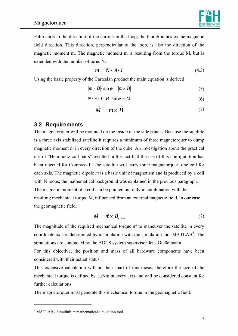
Palm curls in the direction of the current in the loop; the thumb indicates the magnetic
field direction. This direction, perpendicular to the loop, is also the direction of the
magnetic moment m. The magnetic moment m is resulting from the torque M, but is
extended with the number of turns N.
IANm ⋅⋅= (4.3)
Using the basic property of the Cartesian product the main equation is derived
BmBm ×=⋅⋅ φsin (5)
MBIAN =⋅⋅⋅⋅ φsin (6)
BmM ×= (7)
3.2 Requirements The magnetorquer will be mounted on the inside of the side panels. Because the satellite
is a three axis stabilized satellite it requires a minimum of three magnetorquer to dump
magnetic moment m in every direction of the cube. An investigation about the practical
use of “Helmholtz coil pairs” resulted in the fact that the use of this configuration has
been rejected for Compass-1. The satellite will carry three magnetorquer, one coil for
each axis. The magnetic dipole m is a basic unit of magnetism and is produced by a coil
with N loops, the mathematical background was explained in the previous paragraph.
The magnetic moment of a coil can be pointed out only in combination with the
resulting mechanical torque M, influenced from an external magnetic field, in our case
the geomagnetic field.
earthBmM ×= (7)
The magnitude of the required mechanical torque M to maneuver the satellite in every
coordinate axis is determined by a simulation with the simulation tool MATLAB5. The
simulations are conducted by the ADCS system supervisor Jens Gießelmann.
For this objective, the position and mass of all hardware components have been
considered with their actual status.
This extensive calculation will not be a part of this thesis, therefore the size of the
mechanical torque is defined by 1µNm in every axis and will be considered constant for
further calculations.
The magnetorquer must generate this mechanical torque in the geomagnetic field.
5 MATLAB / Simulink = mathematical simulation tool

Magnetorquer
8
The intensity of the geomagnetic field is a function of the altitude of the cube which
again is depending on the launcher of Compass-1. The Cube Sat launchers usually go
into a sun-synchronous orbit with an altitude of 500-800 km and an inclination of up to
98 degrees. The design altitude of Compass-1 was defined in the phase B study as 600
km. [1]
The cross product ( earthBmM ×= ) in scalar solution denotes the angle between two
vectors. With the knowledge of using three magnetorquer is the angle between the
generated magnetic moment vector and the geomagnetic field intensity vector defined
as °= 90ϕ . The produced magnetic moment m is calculated with the multiplication of
the current I, the number of turns N and the enclosed area A established in the previous
paragraph:
AINm ⋅⋅= (8)
A CubeSat has strict limitation on available power and maximum weight for all
hardware components. Having in mind an average of 1 Watt that is constantly available
for the total system, the coil has to be supplied with 250mW. The configuration of the
coils allows an operation of two coils at the same time, but including a restriction that
the coils are not in use constantly.
The mass budget is derived from the literature [3] and from the AAU CubeSat group.
[4] The budget was defined during the development of the Phase B study of this student
project with 20g for each coil.
The available space and size of the coils have been limited by the structure team; details
are shown in the table 3-1.
Parameter Symbol Value Unit
Max width b 74 mm
Max height h 83 mm
Max cross sectional width d 2,1 mm
Max cross sectional height sh 5 mm
Total mass limit Mges 60 g
Coil mass limit Mc 20 g
Table 3-1: Physical design dimensions
The maximum width and this altitude define the physically available area. The cross
sectional breath was defined in the early stage of the project. Other components e.g. the
coil holder; have been designed under consideration of this definition. The cross
sectional altitude can be designed in sizes between 1 and 6 mm.

Magnetorquer
9
The operational temperature was analyzed in another diploma thesis of the Compass-1
group member, who has determined the first thermal result considering the status of the
hardware components in September 2004. [5] The analysis was executed with the
thermal calculation tool ANSYS6. The results was a set of temperature distributions
during earth orbits and temperature ranges for specific hardware components, e.g.
camera, battery, solar cells, electronics and structure. Table 3-2 displays the defined
operational temperatures, which consider the estimation about the self heating of the
wire and the position of the coil inside the panels. They are results of the analysis
performed:
Minimum temperature T min -50 °C Nominal temperature T Nominal 20 °C
Maximum temperature T max 100 °C Table 3-2: Defined operation temperatures
3.3 Design The coils will require a significant portion of the critical mass and power budgets of the
ADCS subsystem. The design of the magnetorquer is following the “as simple as
possible” principle. As mentioned before the magnetorquer are nothing else than copper
wire wound into large loops. The mass of every coil is calculated using the following
expression:
wwc aCNM ρ⋅⋅⋅= (9)
The total mass of a magnetorquer is depending on the number of turns N, its average
circumference C, which is depending on the mechanical dimensions, the cross sectional
area wa of every single wire and the material density wρ of the used wire.
Parameter Symbol Value (Cu) Value (Al) Unit
Material density ρ 8.93E-03 2.7E-03 g/mm^3
Material resistivity σ 1.55E-05 2.5E-05 Ώmm
Temperature coefficient of resistivity α0 3.90E-03 3.90E-03 1/K
Table 3-3: Wire data for copper and aluminium
The wire will be operating under space conditions, relatively quick changes of working
temperatures, which result in a design which considers the “worst case” scenarios. The
resistance of the wire is a function of the operating temperature and the used wire
dimensions.
6 ANSYS / Thermal simulation tool

Magnetorquer
10
waTCNR )(σ⋅⋅= (10)
)1()( 00 TT ∆⋅+⋅= ασσ (11)
A 5 V power supply is considered in the magnetorquer development.
The power stage (Coil Driver) used to control the magnetorquer will cause an additional
power loss, this will be considered separately after being chosen and designed.
The power loss is considered with an additional function of about 200mV for these
calculations. The dissipated electrical power is described by the following electrical
equation:
RIIUP c ⋅=⋅= 2 (12)
The produced magnetic moment m is calculated with the multiplication of the current I,
the number of turns N and the enclosed area A affiliated in the chapters before:
AINm ⋅⋅=
With the equations (9) till (12), the power consumption of a single coil is expressed as: 22
⎟⎠⎞
⎜⎝⎛=
AC
Mm
PC
Twσρ (13)
The ambition is to ensure the efficiency of the coil, with consideration of mass and
power consumption. It becomes obvious at this stage that the design process will be a
trade-off between mass and power consumption. It is possible to reduce the weight, by
reducing the number of turns but the power consumption will increase, and vice versa.
Solving equation (13) for the achievable magnetic moment m yields
Tw
c PMCAm
σρ= (14)
The maximum of this equation is given with a minimized product of the material
density (ρ) and the material resistance Tσ . This product can be minimised by the choice
of adequate wire material.
As wire material options we have the choice between copper and aluminium wire.
Copper has the lowest resistance, but aluminium has the lowest resistance-density
product. Due to the fact that volume is expected to be more of a constraint than mass,
copper seems the obvious choice.
It should be noted that the design of the coils does not only depend on the required
mechanical torque and the selected number of turns. The commercial availability of the
right wire with the qualified wire properties is becoming a more important argument.

Magnetorquer
11
The first research yielded a contact with the biggest wire supplier in Europe,
Elektrisola7. The company is characterised by a divers set of applications; many
different wire variants are in use in many different engineering areas, e.g. in cars,
computer, watches etc.
A large variety of available copper wire with a suitable insulation as well as the low cost
outweighs the variety of the available aluminium wire.
After several discussions with the supplier about the available wire properties two wire
types have been selected types based on the European IEC 60317 standard [6] the
copper wire type Polysol 180 and the ML 240 type copper wire. [7] The special copper
wire ML 240 is qualified for military and space applications, whereas very high cost is
linked to such a high quality wire type. In addition, the wire type ML 240 is produced in
the U.S. and can be delivered only on special order. This has resulted in the fact that the
only available wire type can be matched with the Poysol 180 type wire.
Polysol 180 is a self-bonding wire available from the diameter 0.1mm through 0.5mm.
For this reason of the right wire diameter, the environmental conditions need to be
included into the mathematical design of the “rectangular” coil.
The intensity of the geomagnetic field is a function of the altitude of the orbit. For the
determination of the geomagnetic field intensity is the radius considered from the geo
centre with orbitearth hRR += . With the constant sizes of the earth radius 6371=earthR km
the dipole moment of the earth as 221096.7 ⋅=em Am² and the magnetic
permeabilityAmVs7
0 104 −⋅⋅= πµ .
³40
min, Rm
B eearth ⋅⋅
⋅=
πµ
(15)
Minimum geomagnetic intensity, at 600 km altitude is calculated as 51035.2 −⋅=earthB T.
This magnetic moment needs to be generated at any scenario, with the limited amount
of power. For the acceleration of the design task, an Excel programme was developed.
The programme considers all requirements and delivers the necessary parameter, the
wire diameter and the number of turns.
As explained before, the design process is a trade-off between mass and power
consumption. Therefore the minimum required mass is determined first with the
following expression.
7 www.elektrisola.com

Magnetorquer
12
PAmCM C
202 ρσ⋅⎟
⎠⎞
⎜⎝⎛= (16)
The minimum required mass is determined at 20 °C, with the magnetic dipole moment
²1026.4 2 Amm −×= , the maximum available power mWP 250= and the mechanical
dimensions mmC 294= ²6142mmA = .
The first calculations have resulted in a minimum required mass of 3,2 gram for each
coil. With the knowledge about the minimum mass, the minimum wire cross section
area is determined with the following expressions:
PUR coil min,
2
max = (17.0)
min,
maxmin,2
maxw
coil
anC
PUR
σ== (17.1)
ρ
σ maxmin
min,min,
1 PMU
a c
coilw = (17.2)
The minimum cross section area ²00818.0min, mmaw = of the wire delivers the minimum
wire diameter as shown in the following matrix.
Wire Diameter [mm]
Cross Area
[mm^2]
Diameter incl. Insulation [mm]
Area incl. Insulation
[mm^2]
Filling Factor
0,100 0,007854 0,108 0,0091609 9124
0,106 0,008825 0,115 0,0103868 8154
0,110 0,009503 0,119 0,0111220 7571
0,112 0,009852 0,121 0,0114990 7331
0,118 0,010936 0,128 0,0128680 6627
0,120 0,01131 0,13 0,0132732 6431
0,125 0,012272 0,135 0,0143139 5934
0,130 0,013273 0,141 0,0156145 5454
0,132 0,013685 0,143 0,0160606 5307
0,140 0,015394 0,151 0,0179079 4775
0,150 0,017671 0,162 0,0206120 4165
0,160 0,020106 0,172 0,0233522 3686
0,170 0,022698 0,183 0,0263022 3250
0,180 0,025447 0,193 0,0292553 2931
0,190 0,028353 0,204 0,0326851 2618
0,200 0,031416 0,214 0,0359681 2386
Table 3-4: Datasheet of available Copper Wire IEC 60317 [6]
Magnetorquer
13
With the knowledge about the available wire displays that every wire diameter bigger
than 0.106 mm can be used for the magnetorquer of Compass-1.
T
PCNCAm
σ⋅⋅⋅
= wa (17.3)
Equation (17.3) displays the direct proportionality of the magnetic moment to wa
with constant number of turns N, constant circumference C and constant area A.
After selecting a suitable wire diameter, the new wire cross sectional area needs to be
implemented for the number of turn calculations. Modulation of equation (17.2) delivers
the required number of turns.
ρavailw
c
CaMN
,
= (17.4)
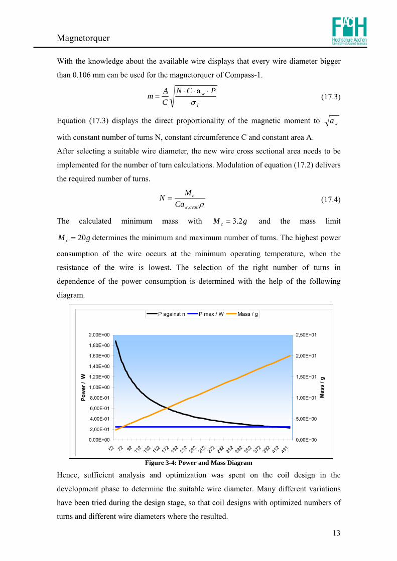
The calculated minimum mass with gM c 2.3= and the mass limit
gM c 20= determines the minimum and maximum number of turns. The highest power
consumption of the wire occurs at the minimum operating temperature, when the
resistance of the wire is lowest. The selection of the right number of turns in
dependence of the power consumption is determined with the help of the following
diagram.
Figure 3-4: Power and Mass Diagram
Hence, sufficient analysis and optimization was spent on the coil design in the
development phase to determine the suitable wire diameter. Many different variations
have been tried during the design stage, so that coil designs with optimized numbers of
turns and different wire diameters where the resulted.
0,00E+00
2,00E-01
4,00E-01
6,00E-01
8,00E-01
1,00E+00
1,20E+00
1,40E+00
1,60E+00
1,80E+00
2,00E+00
52 72 92 112
132
152
172
192
212
232
252
272
292
312
332
352
372
392
412
431
Pow
er /
W
0,00E+00
5,00E+00
1,00E+01
1,50E+01
2,00E+01
2,50E+01
Mas
s / g
P against n P max / W Mass / g

Magnetorquer
14
Figure 3-5: Design results
The design results shows the varieties of winded coils with constant mechanical size
established by increasing the wire diameter by the smaller wire. An increase of the
magnetic moment an increase of the power consumption and at the same time
depending on the wire diameter is displayed.
The result shows a margin percentage of the generated magnetic moment, of up to
120%. Despite an overrun of the power consumption value 9 stands out compared to the
other values, whereas the power consumption “change” to an adjustable function. The
power consumption is drawn to the temperature limit at -50°C. The next matrix displays
a possible coil design: Parameter Symbol Value Unit
Number of Turns n 400 -
Bare wire diameter dw 0.15 mm
Mass of one coil Mc 19.20 g
Current through coil I (20°C) 41.30 mA
Magnetic dipole moment m 9.19E-02 A*m^2
Needed cross section area Ac 9.604 mm^2
Power consumption (223K) P 256.5 mW
Power consumption (293K) P 202.3 mW
Coil resistance @ -50°C R-50 93.55 Ω
Coil resistance @ 20°C R20 116.21 Ω
Coil resistance @ 100°C R100 161.53 Ω
Table 3-5: Coil design result
Design Results Parameter Symbol Value 7 Value 8 Value 9 Unit
wire diameter d 0,106 0,13 0,15 mmnumber of turns n 830 553 416
mass of one coil Mc 19,969 19,995 19,968 gneeded cross section area Ac 10,179 10,139 9,988 mm²
nominal current I (293K) 9,85 22,23 39,35 mAsupply voltage U 5 5 5 V
Power consumption P(223K) 65,95 148,87 263,46 mW
magnetic dipole moment m 4,86E-02 7,07E-02 9,41E-02 Am²
Margin of m4,26E-02 14,08% 65,96% 120,89%
Margin 4.26 E-02 Am² 14.08 % 65.96% 120.89%
N

Magnetorquer
15
3.4 Production For the production of magnetorquer at universities several possibilities exist.
Maybe some few universities have very good connections to their national space
agencies so they can get the knowledge of producing space qualified magnetorquer, or
even can get a installable magnetorquer for their cube.
Universities are able to cooperate with national space agencies and specialised
companies, but not every university has existing connection to specialized companies.
A project like Compass-1 was initiated at the FH Aachen for the first time. It is
financially supported by the DLR (German Aero Space Centre), the FH Aachen, the
Ministry of NRW (Nordrhein-Westfalen) and ESA (European Space Agency).
About 4 weeks have been invested on research activities, which have resulted in
contacts with diverse companies and universities, especially to CHK Wickeltechnik8.
This company is producing coils for any conceivable application. Several telephone
calls and e-mails have resulted in the best offer of CHK Wickeltechnik. The company
offered a production of six coils for a net cost of about 2000 – 3000 Euro. This
contained the coil mould, the wire material and production costs, so that every new coil
order will get charged with the wire and production expenses.
Considering the quality aspects, the development aspects in combination with the
educational aspects and especially the financial aspects approves an in-house production
of electromagnetic coils. The in-house production of coils will allow high flexibility; the
production of magnetorquer can be converted into a relatively inexpensive procedure
compared to a company production. Therefore an own automated coil winder needs to
be designed, developed and produced. Prior to the design tasks, a feasibility study was
accomplished. The study has shown that the coil winder can be designed with the same
software tool used for the design of the satellite structure, CATIA. Afterwards, the
production of the mechanical hardware can be accomplished at the own mechanical
workshop. The in-house production of magnetorquer requires many different facilities
and components. First of all the wire needs to be selected and ordered from the supplier,
so that the available wire diameter can be taken into account throughout the coil winder
design. Remembering that Compass-1 is a student project with very limited financial
budget it was agreed upon with the company Elektrisola that two different diameters
can be chosen.
8 www.chk-wickeltechnik.de

Magnetorquer
16
Figure 3-6: Bonding wire type S180
Elektrisola has spent surprisingly two 2 kg coils with special bonding wire of the wire
type S180 with the chosen nominal diameter of 0.15mm and 0.16mm displayed in the
picture. For further production aspects all available facilities will be used for the
production of the magnetorquer. The electrical workshop in our own laboratory will be
used for different electrical activities. Moreover a vacuum chamber, also a part of our
own laboratory will be used for the space qualification of the coil.
But as a next challenge the design of a moderate-complexity coil winder will be
presented in the next chapter.

Coil Winder
17
4 Coil Winder The following chapter describes the construction of the magnetorquers; which was
theoretically designed in the chapter before.
To wind the coil manually with an easy mould; i.e. 4 screws mounted on a flat board,
seems as the fastest and easiest way at first sight.
By considering the electrical specification, it might be right, but due to the fact that
three identical coils with a very small wire diameter and a relatively high number of
turns will be integrated are getting the mechanical dimensions even more attention.
It should be noted that the coils will operate under space conditions, for this aspect the
coils need to pass all space qualification tests later on. Compass-1 space qualification
tests include a vibration test of the whole cube, a thermal test and finally a vacuum test.
In the design status of the Coil shape it becomes obvious that the manufacturing of three
coils which will produce a mechanical torque under space conditions requires a
development of a customized coil winder.
The coil winder guarantees, a higher quality of produced coils compared to the manual
wound coils.
4.1 Layout To wind wire automated into a coil; different hardware components need to be
designed.
First of all a coil mould is needed. The mould should be integratable into a winding unit
with an integrated drive mechanism. To wind an accurate coil, a tracking package seems
to be useful. For monitoring the wire tensions a force measuring unit need to be
implemented, without integrating additional stress. Resulting from the not round coil
architecture the wire will be under different stresses during the winding, to distribute
these stresses; pulleys can be used. To finish the open cycle and in consideration of
producing diverse coils a wire stock need to be generated and implemented.
The simplified layout which is shown in Figure 4-1 depicts the architectural concept of
the main components of the winder.
The winder can be splinted into seven mechanical areas as follows a coil mould, a
winding unit, a track package, a force measuring unit, the pulley´s, the wire holder and
the base plate.

Coil Winder
18
Figure 4-1 Winder architecture concept
The mechanical dimension of the coil mould is driven by the mechanical layout
dimension of the magnetorquer. The maximum allowed dimension of the magnetorquer
is given the available structural dimension of the cube; as 83 x 74 mm². From the
theoretical cross section altitude of the coil with 5mm results the dimension of the coil
mould with 73 x 64 mm².
The thickness of the coil was defined at 2,1mm. The shape of the coil mould needs to be
rectangular and the mould needs to be hinged in the coil winding unit. The material and
the mechanical dimension of the coil mould will be specifically discussed in an extra
paragraph.
At this design stage the important aspects of the coil mould is expressed as:
• the mould has been integrable into the coil shape
• pivoted in any preferred way.
Next to the pivoted coil mould; the design of the other coil winder components must
consider a constant stream of wire.
Figure 4-2: Coil Mould Sketch
+=

Coil Winder
19
The knowledge of the coil shape and the noted production setup (the rotation) need to
be deferred at this stage of the design status.
Usually mechanical constructions are designed from the inside (main task) of the body
to the outer surfaces, some winding subsystems are designed in consideration of this
“construction Rule”.
To get more clearness about the function of the respective mechanical components the
design of the winder is explained from one geometric sequence to another, starting from
the fundamental hardware, the base plate.
All design and development activities are generated with 3D construction software
CATIA V5 R13. The software CATIA V5 allows a full design and development of all
mechanical parts including an assembly mode where all mechanical parts can packetize
and assimilate with each other.
During the design and development phase and later on with the possible modifications
phase; this software accelerate the different work packages for hardware production.
Figure 4-3: Catia V5 R13 screenshot of Compass-1 (EM)
4.2 Requirements The design of the coil winder considers a modular mechanical body to provide a flexible
configuration for any changes during the development phase.
The coil winder assumes in the whole design and development phase, in consideration
of the production expenses and the financial budget, as simple as possible, without
losing the focus for a sensitive winding tool an easy hardware construction.

Coil Winder
20
The important recommended values for all hardware components is driven by the used
copper wire. The maximum tension of the copper wire is appointed by the isolation
characteristics of the copper wire. [6]
To manufacture high quality coils, the packing density of the coil needs to be as high as
possible, so the wire needs to be winded as constant as possible. A high packing density
is achievable with a combination of a relative high preliminary tension, in view of the
coil volume and a good wire guidance.
The guidance needs to operate synchronously with the winding unit to appoint the
required sensibility the increment of the guidance needs to be in the area of a quarter of
the used wire diameter.
Next to all material limits the winder needs to be designed including as much as
possible commercial of the self products (COTS). COTS products are performed on the
basis of low cost, commercial availability and reliability hardware.
The material of the designed mechanical parts will be standard aluminium. Aluminium
compared to steel has the advantage that the mechanical parts are not oxidizing and in
the same time aluminium is easier and faster to handle at the FH mechanical workshop.
4.3 Hardware Design & Development
4.3.1 Base Plate The base plate should offer a flexible modular platform, which allows less restraint for a
general design. For the layout of the base plate different opportunities are given:
A base plate could be manufactured at the FH mechanical workshop, therefore all
hardware interfaces including the base plate itself need to be defined from the beginning
of this design task. The same base plate can also be machined also from time to time,
depending on the improvement of the winder. Nevertheless this kind of manufacturing
will take much more production time and furthermore the accuracy of all hardware
interfaces could be imprecise. The base plate should offer a relative flexible design of
the coil winder parts. A modular and at the same time a relative flexible base plate is in
use at usual CNC milling machines, a so called T groove profile plate. This kind of base
plate will be the best solution, and in addition the T groove plates are offered very cheap
by the company ISEL9.
9 www.isel.com

Coil Winder
21
At the home page of the provider several aluminium profiles are displayed, which are
actually differentiated from the mechanical sizes and their application area.
A good solution for the required coil winder modularity is given with aluminium PT-
Profiles. [8]
Figure 4-4: Different PT-Aluminium-Profiles
The PT-Profiles require universal surfaces which are naturally anodized, thick walled,
without distortions, dimensionally stable and double sided mill cut.
The PT 25 Profile offers an middle flute distance of 25 mm with a constant height of 20
mm and is in its width available in 125mm steps.
PT 25 Profile Catia Model (front view)
Figure 4-5: PT 25 Profile 3 D Catia Model

Coil Winder
22
T-Groove blocks show a good opportunity for the interface between the T groove plate
and the different hardware parts. The T-Groove blocks allow a flexible interface with
only one condition, that all interfaces need to be established with M 6 screws, therefore
all trough hole drills need to be laid out for M6 screws DIN EN 20273 with the fine
diameter of 6,4mm or middle diameter of 6,6mm.
This T groove screw nuts are offered relatively cheap from the supplier Maedler10. In
consideration of the hardware accuracy the DIN EN 20273 middle norm was chosen for
further model layouts.
Figure 4-6: T Groove Screw Nut M6 DIN 650
4.3.2 Wire Carrier / Wire Cover Brake
Figure 4-7: Wire Stock as 3 D Model
The main function of the wire stock coil is to deliver constant wire for more than only
one coil. This body is build up with two sidewalls with integrated FAG bearings with a
thread bolt (spindle) where the wire stock cover can mount on. The cover is fixed with a
10 www.maedler.de

Coil Winder
23
customized screw nut, which helps to centre the wire cover compared to the thread bolt.
This sanction guarantees the concentricity of the system. Both ends of the “M 10”
threaded bolt are reduced to a size of 8 mm and are secured against horizontal
movements with usual retaining rings. The wire at the wire stock transacts the wire
constantly so it decreases its circumference constantly, therefore a relative flexible
transaction level (high) is implemented into the system. The limiter is constructed with
a standard aluminium rod with integrated FAG bearings and a small standard spindle
with a diameter of 5 mm. This spindle is also secured with retaining rings against
vertical movements.
To avoid an uncontrolled unwinding of the wire, a friction brake needs to be
implemented. The wire brake has the function to hold an initial load of the wire at a
constant level. With the consideration of the small wire diameter and its allowed forces,
it was decided to design a wire brake, which allows a small friction force resulting in a
low brake momentum at the wire stock coil. All commercial available brakes, i.e. drum
brakes, are either not proper for this force area or show the problem that the brake is not
adjustable very fine for this use. Therefore a mobile unit was designed where easily a
spring steel rod is integrated. Usual screws are used for folding the spring steel rod and
transforming a frictional force to the wire carrier.
Figure 4-8: Wire Carrier & Wire Brake mounted on the base plate

Coil Winder
24
After construction of the wire carrier part, the wire needs to appease during the recoil
movements. A reassurance of the system can be managed by deflection pulleys in
special configurations.
4.3.3 Pulley
Figure 4-9: Deflection pulleys mounted on an aluminium rod with different offsets
Relative big buffers with different configurations are needed so that all wire movements
can be distributed and controlled. The first movement which needs to be under control
is the recoil movement of the wire which is moving from one side to another.
The second movement is caused by the rectangular coil mould, which affects the wire
with different pull forces. The deflection pulleys have the function to turn round the
wire and therefore generate a buffer for the agent forces. The same pulleys, but with a
“smaller” offset of the rods (Figure 4-9) in a different configuration are used to appease
the recoil movement of the wire. The pulleys are mounted on standard aluminium rods
and these again are screwed on a socket.
The deflection rollers are deliverable in four different variations. [9]
The variations differentiate only in the milled groove. The deflection roller are
deliverable with edged groove, V-grooved, round groove and without any groove. This
groove enables a safe wire stream at a defined height. The next figure shows the offered
pulleys from the bearing provider GedeHemer11.
11 www.gedehemer.com

Coil Winder
25
Figure 4-10: Deflection pulleys
The size of the groove is depending on the size of the wire and the wish of the
customers. In order that the guided wire is not getting extra punctual stress, the pulley
with an outer diameter of 12 mm with a round groove of 0.25 mm was selected.
Figure 4-11: Pulleys placed on the base plate

Coil Winder
26
4.3.4 Guidance
Figure 4-12: Redesigned guidance unit Figure 4-13: First design of the guidance
The manufacturing of high quality coils with a high packing density requires guidance
of the wire during the winding process. The guidance needs to be very accurate, because
of the very thin copper wire with a nominal diameter of 0.15mm . This means that the
guidance accuracy needs to be at least the wire diameter, better a quarter of the wire
diameter. To guarantee such guidance special units, possibly COTS products, needs to
be implemented into the guiding unit. The unit needs to reciprocate the wire “only” in
the horizontal axis but with a very high accuracy. A good solution for a reciprocate
movement is given with a threat rod with an integrated interface, which transform the
rotation into an accurate horizontal reciprocate flow.
Figure 4-14: Moved threat rod with interface
Threat rod Special guidance

Coil Winder
27
The guidance needs high precision, therefore the unit needs to be best with ± zero
tolerance. The practice shows that high quality COTS products are also relative high in
cost. For this reason some companies have student discounts up to 20%. Not infrequent
the companies offer their different possibilities to support student activities as best with
a complete sponsoring of the hardware product.
Anyway, a very fine guidance is established in every CNC milling cutter with special
ball screw spindles [10].
Figure 4-15: Several spindles with different guide interfaces
The special ball screw spindles offer high tracking precision which are not depending
only on the spindle itself, but rather on the quality of interfaced units.
The spindles are usually delivered in combination with the adequate bearings and every
supplier offers also variations of guide blocks, gear units and drive mechanisms. The
only limit for ready units is set actually with the financial budget. Ready units can costs
up to 1000 Euro and more therefore this unit is setup with cheaper COTS products but
with similar functions.
Stepping motors as the drive mechanism offer compared to the usual electric motors
(DC motors) the possibility of linear guide by dividing a whole circle of a rotation into
steps. The drive mechanism could be designed also with a DC motor but in combination
with a very expensive measurement technology, e.g. Exposed Linear Encoders from the
supplier HEIDENHEIN12.
The “Body” of the guidance is designed around the special spindle. The body is
constructed with two main blocks and two sidewalls. The special screw spindle bearings
(blue) are integrated into both sidewalls for an easy integration of the spindle. The main
block offers the integration of special guide rails, which are needed in consideration of
the horizontal movement.
12 www.heidenhain.de

Coil Winder
28
Figure 4-16: Base construction with guide rails Figure 4-17: Interface unit
To transfer the spindle movement to a guidance movement an extra interface is
designed. The interface is built-on with two perpendicular screwed plates, one plate
interfaces with the spindle and the other plate interfaces with the “roll board”.
The “roll board” enables easy integration of two perpendicular guidance rolls and
creates the interface between the guidance unit and the guided wire.
Before the “roll board” can be designed into a final version, the kind of usable rolls
needs to be identified, while every roll offers different surface properties.
A research about guidance rolls has resulted that different “rolls” exist. Just to name a
few: Guide rolls, cone rolls, straightening rollers, roller crosses, guide units and so on.
[9]
The last two expressions are actually ready build units, where different rolls are in use.
Considering the financial budget of the winding unit and the view of a new design
possibility, the ready units will require too much of the available budget, therefore the
different rolls should help to solve the guidance design. The next figure shows the
offered rolls from the bearing provider GedeHemer13
13 www.gede-hemer.de

Coil Winder
29
Figure 4-18: Guide rolls, Cam Followers, Roller Followers
A good solution is given with the guide rolls Type 2, these rolls are screw-mountable
from one side, which is advantageous for integration aspects and in addition these rolls
are in use for similar uses in production lines of big winding companies.
Figure 4-19: Roll board
During the development phase of this unit, the Linear Actuator [11] have been
referenced by a Compass-1 team member. The institute which he is working for is
using this actuator for “hexapod” applications.
The linear actuators compromise actually a stepping motor with a small increment, a
high tracking guidance with an easy assembly possibility.

Coil Winder
30
Figure 4-20: Linear Actuator LC 15
This unit is the smallest commercially available linear actuator in the world, with a step
accuracy of 0.02mm per step. The drive mechanism of this unit compromises a stepping
motor with also 200 steps per revolution.
The unit is used for medical instrumentation, optics, machinery automation and many
more automated devices which require precise remote controlled linear movements in a
very small package size. [11] This unit combines, compared to the other solution, the
threat rod with the special interface, the FAG bearings and a clutch with a
corresponding stepping motor. These huge advantages will increase the quality of this
unit by reducing the costs in the same time.
Hence these facts drove this unit to a redesign. At the redesign of the guidance unit all
designed parts, except the basic unit, have been transferred to the new required unit.
The huge advantages of this COTS product caused a redesign of the guidance unit.
Figure 4-21: Coil winder model with additional the guidance unit

Coil Winder
31
4.3.5 Winding Unit The main design idea of this unit considers the easy integration and later an easy
demounting of the coil mould for further activities. An easy unit can be established e.g.
with an easy construction where every part fits into only one position. The winding unit
is built around the coil mould and is built-on a flat base plate. The hardware offers a
static defined Holder (figure left) where the coil mould can easily installed.
Figure 4-22: Winding unit mounted on a flat plate
The holder itself is actually nothing else than a sidewall with an integrated FAG
bearing, with a spindle which is secured against the vertical movement with a retaining
ring. To get a mechanical contact for rotation aspects, between the coil mould and the
shaft; an easy solution is to impose a brass sleeve over the shaft, which is locked with a
pin. It should be noted that the rotation frequency will not be so high compared to long
run production.
To avert a handicap between the shaft and the bearing, the shaft diameter (red) must be
smaller than the diameter of the inner ring of the FAG bearing.
The coil mould and the shaft are made up of different materials to block the internal
wear out. The shaft is made up of brass material and the coil mould of standard
aluminium.
Next to the locking devices the pin has an additional function. It is helping to create an
interface between the coil mould and the mechanical drive (Stepping motor).
To accomplish the interface a slotted hole needs to be milled into the coil mould where
the pin is fitting in. In addition the interface will be greased with standard machine oil,
lubrication grease, for a better integration and removal of the adequate coil mould.
The design of the spindle considers the bending loads causing from the weight of the
coil mould.
Coil Winder
32
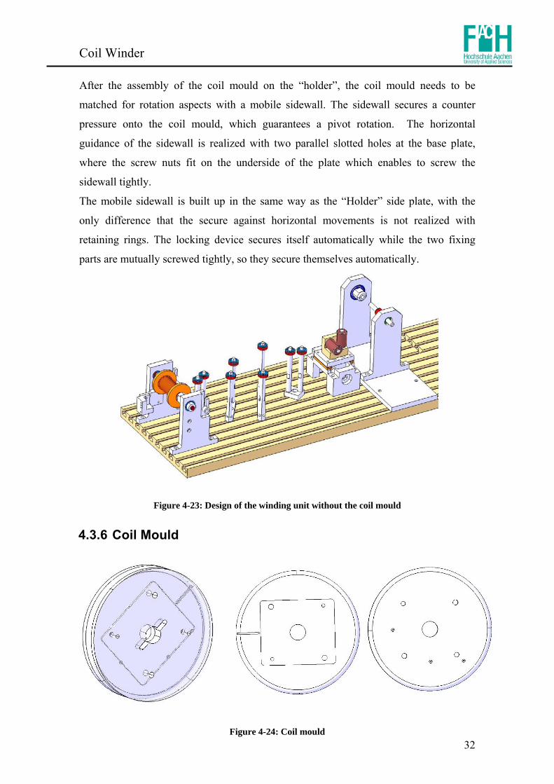
After the assembly of the coil mould on the “holder”, the coil mould needs to be
matched for rotation aspects with a mobile sidewall. The sidewall secures a counter
pressure onto the coil mould, which guarantees a pivot rotation. The horizontal
guidance of the sidewall is realized with two parallel slotted holes at the base plate,
where the screw nuts fit on the underside of the plate which enables to screw the
sidewall tightly.
The mobile sidewall is built up in the same way as the “Holder” side plate, with the
only difference that the secure against horizontal movements is not realized with
retaining rings. The locking device secures itself automatically while the two fixing
parts are mutually screwed tightly, so they secure themselves automatically.
Figure 4-23: Design of the winding unit without the coil mould
4.3.6 Coil Mould
Figure 4-24: Coil mould

Coil Winder
33
The mould simply consists of two round plates, one plate to wrap up the wire and a
second plate to generate the counter plate, with three small drills to thread the wire to
the desired position. These two plates are fixed with two converse oriented dowel pins
and are also screwed with two converse oriented hexagon socket screws.
In order not to destroy the wire during the winding a round winding mould with
rounded edges with an integrated rectangular coil mould was designed. The edges of the
rectangular coil mould, at the inside, are also rounded with a minimum size of 3 mm.
The rectangular coil mould with 73 x 64 mm² is resulting from the theoretical coil
thickness of 5 mm.
The coil mould is built up with standard round aluminium which is relative easy to
manufacture and in addition aluminium shows a relatively good thermal character. This
thermal character will be important for further connection activities, whereas the
bonding will be established by heating up the wire.
The coil will have a thickness of 2,1mm which results from 2 mm winding place, which
was available at the cube, plus a safety margin of 5 %. The margin will upgrade the
connection quality of the coil on the panels, due the fact that the coil holder will have
only 2.0 mm space. The small difference will cause a small squeeze effect at the coil
itself but without any mechanical deformations.
Figure 4-25: Design result of the coil winder

Coil Winder
34
4.3.7 Force Measuring Unit
Figure 4-26: Force measuring unit
The force measuring unit is an additive unit which is designed to monitor and record the
wire forces during the winding. The tension of the wire has in the calculation no direct
influence to the electrical characteristics, but to the mechanical dimensions. Low
tensions cause an unconstant dimension of winded coils; the result of the first
prototypes will confirm this proposition.
The maximum force limit is governed by the wire isolation, which is around 1.5N. The
force measuring is challenging the design task with a transferring of the horizontal wire
stream forces into a digital signal, without temper the measuring. Electrical units i.e.
potentiometers can help to transfer mechanical movement to a digital signal, but the
friction of the potentiometer transforms this solution to an inoperative solution.
The measuring unit should introduce a very small error into the measurement otherwise
it makes no sense, especially at this small measurement range, to record the wire
tensions. The recording of the wire tensions at big cable companies are measured with
special instruments. This instruments use the measuring principle of a tackle which
creates the basis for the design of this unit.
The wire needs to be positioned and controlled before and after the force measuring
unit, in order to carry out the measurement inside the tackle.

Coil Winder
35
spring
wire mobile unit
Figure 4-27: Tackle principia
The wire stream forces are transformed with the tackle design into a horizontal
movement, where the middle pulley is mounted on a fine guide rail with a low self
locking. With the aid of this mobile pivoted roll, the wire force changes are visible,
assumed that this pivoted roll is “fixed” to another system. A fix and in the same time
mobile roll is established by the integration of a spring into the fastener cable. This
arrangement enables the transformation of the horizontal drive into a rotation, assuming
that the referenced system is also pivoted.
A pivoted measuring unit, an incremental driver from the model making have been
recommended for this special feeding. With the known spring stiffness the wire forces
are recordable from the proportion between the rotation-angles enabled from the
expansion of the spring. The incremental driver has in case of an angle measurement a
unique resolution up to a half degree. The compound between the pivoted roll and the
incremental driver is designed flexible, so that during the manufacturing the right spring
can be chosen and integrated easily.
Figure 4-28: Coil winder with force measuring unit

Coil Winder
36
4.3.8 Electrical Drives and Measuring Unit During the design task of the coil winder the electrical drives have been considered. The
electro-mechanical units are stepping motors; stepping motors fill a unique niche in the
motion control world. These motors are commonly used for measurement and control
applications. Sample applications include CNC machines and volumetric pumps.
Several features common to all stepper motors make them ideally suited for these types
of applications. These features are as follows:
1. Open Loop Positioning - Stepper motors move in quantified increments or
steps. As long as the motor runs within its torque specification, the position of
the shaft is known at all times without the need for a feedback mechanism.
2. Holding Torque - Stepper motors are able to hold the shaft stationary.
3. Excellent Response - to start-up, stopping and reverse movements.
There are three basic types of stepping motors: permanent magnet, variable reluctance
and hybrid. Permanent magnet motors have a magnetized rotor, while variable
reluctance motors have toothed soft-iron rotors. The stator or stationary part of the
stepping motor holds multiple windings. The arrangement of these windings is the
primary factor that distinguishes different types of stepping motors from an electrical
point of view. From the electrical and control system perspective, variable reluctance
motors are distant from the other types. Variable Reluctance Motors have three to five
windings connected to a common terminal.
Unipolar stepping motors are composed of two windings, each with a center tap. The
center taps are brought outside the motor as two separate wires as a result unipolar
motors have five or six wires. The center tap wires are tied to a power supply and the
ends of the coils are alternately grounded.
Bipolar stepping motors are composed of two windings and have four wires. Unlike
unipolar motors, bipolar motors have no center taps. The advantages of not having
center taps is that current runs through an entire winding at a time instead of just half of
the winding. As result, bipolar motors produce more torque than unipolar motors of the
same size. The draw back of bipolar motors, compared to unipolar motors, is that more
complex control circuitry is required by bipolar motors.
The selected stepping motor for the drive mechanism of the coil winder offer the
possibility to share a whole revolution into 200 steps ore more.
The used stepping motor is a unipolar motor but used as a bipolar stepping motor,
which increase the rotation torque of the stepping motor.

Coil Winder
37
Figure 4-29: Bipolar stepping motor Figure 4-30: Incremental driver, rotary encoder
The drive mechanism of the guidance unit is realized with the Linear Actor LC 15
which is actually also a stepping motor with the respective electrical supply.
The gauge of the force measuring unit is the MATSUSHITA Rotary Encoder. The
datasheets of the used unit have not been found from at the supplier, this could result
from the fusion of the producer MATSUSHITA Electric Works LTD14 by Panasonic15.
Nevertheless this encoder allows a determination of the rotation angle with a resolution
up to 0.5°, depending on the electrical supply. The important features of the encoder are
as follows:
• electrical supply 5 V
• contact less angle determination with a integrated optical encoder
• open collector measurement
• resolution: 360 pulses per rotation
14 http://www.mew.co.jp/e/corp/ 15 http://www.mew.com.br/

Coil Winder Production
38
5 Coil Winder Production
5.1 Technical Drawings Diverse commercial off-the-shelf (COTS) are implemented into the coil winder, to
guarantee a given amount of quality. The remaining units of the coil winder have been
custom-designed and developed at the FH Aachen. Following the coil winder design
and development all unit parts have been drawn as technical drawings which were
required for the production tasks at the own FH mechanical workshop. The technical
drawings are constructed with the same software used for the model design and
development of the coil winder, with CATIA V5 R13.
All drawings are coordinated, so that the required accuracy can be manufactured.
After the drawings of different hardware parts, all drawings have been checked from an
assistant of the FH mechanical workshop. For this project the head of the FH
mechanical workshop has checked all drawings and in addition he was contact person in
charge for manufacturing problems.
After the checks some technical drawings needed to be modified. These small
modifications which are usual at the development of specific parts will be not discussed
in details. The final drawings of the coil winder units are ready for access at the
Appendix –A.
5.2 Material and COTS Orders
After the technical drawings were finished, the needed material has been ordered from
diverse suppliers, depending on the cost. The majority of the coil winder unit parts are
milled from standard 10mm or 12mm aluminium plates, ordered from Olimex16. The
thickness resulted from the column width of the PT25 base plate and the particular
functions. The PT 25 T-groove plate was ordered from the supplier ISEL17. The FAG
bearings the majority of the screws and diverse accessories have been ordered from the
supplier KSA18 in Aachen.
16 www.olimex.de / 17 www.isel.com 18 www.ksa-aachen.de

Coil Winder Production
39
The different pulleys, except of the long roll at the wire carrier are chosen and ordered
from the supplier GEDE Hemer19. The standard 10 mm aluminium sticks and the round
aluminium for the coil mould have also been ordered with the aluminium plates from
Olimex. As written in the production part of this thesis Elektrisola has spent the special
bonding copper wire type S180 in two different types.
The stepping motor of the winding unit, the incremental driver of the force measuring
unit and the three guidance rails were sponsored by a Compass-1 group member. The
Linear Actuator LC 15 of the guidance unit was ordered from the European supplier A-
drive20.
The manufacturing of the coil winder has been carried out at our own mechanical
workshop. The diverse unit parts were constructed and produced with different
dimension limits depending on the function. Details of the manufacturing activities are
displayed by the Appendix-B.
19 www.gede-hemer.de 20 www.a-drive.de

Control Unit Design
40
6 Control Unit Design
This part describes the needed electrical hardware interfaces and their software
programmating. The adjustments like the synchronicity of the driving mechanisms are
integrated into the software. The different automated tasks of the coil winder are split
into the electrical and the corresponding software design tasks. Hardware and software
design (and development) generally goes hand in hand.
However, the software is by nature the more flexible part that can be modified more
easily. Therefore it is very advisable to finish the hardware design first but wait with the
development until the software has advanced far enough, so that modifications can still
be integrated in the hardware design.
The electrical hardware components and the software for this control unit are designed
and developed with the layout software Protel 2005.
The transaction of these activities was actually not part of this thesis but different tasks
e.g. layout, selection, ordering activities have been accomplished in a work group.
The documentation of the generated hardware will be limited in this thesis.
The required functions and the interfaces to the different electrical units have been
layout and defined together.
6.1 Electrical Hardware Design
The design process shall derive a physical architecture from the functional analysis and
requirement allocations. The electrical design of the coil winder is affected by the used
drive mechanisms and the used measurement hardware. The principal design of these
electrical components is shown as follows:

Control Unit Design
41
Figure 6-1: Electrical interfaces of the coil winder
The M1 & M2 in Figure 6-1 represent the stepping motors, M1 embodies the drive
mechanism of the winding unit and M2 the stepping motor, Linear Actuator of the
guidance. The Inc.1 represents the incremental unit used in the force measuring unit, the
second incremental unit was considered for the determination of the total coil length.
The unit was planned for the case that the length needs to be determined, while the main
aspect of the coil is described with its resistance.
The electrical box represents a PCB where different hardware components, e.g. the
MCU, power amplifier or voltage regulator and much more components are soldered
on.
At this stage the decision about the integration of a COTS controller unit for the
stepping motor drive seems to be the best and easiest way. But the consideration of the
gauge an incremental, rotary encoder with a high resolution and the financial budget
have resulted in the decision of the design development and production of the own
controller unit, which combines the control of the used different electrical components.
6.2 Circuit Design The circuit design includes the selection and implementation of necessary parts in order
to adjust the main devices in a proper form, e.g. capacitors, resistors, power amplifier,
reset buttons. It should be underlined that the circuit design activities are the most time
consuming parts of the electrical hardware design.
Coil winder
Inc.2 Inc.1 M 2 M 1
Electrical Box P.C. Power suppl RS 232

Control Unit Design
42
For the selection of the main electrical hardware, the microcontroller unit (MCU), the
required digital pins have been determined.
The triggering of both stepping motors is established by using two stepper driver types
IMT 901 from the supplier Nanotec21, which require seven digital I/O pin per driver.
The incremental drivers or rotary encoders require three digital I/O pins each.
It was decided to configure the board for a stand alone function, therefore an interface
for a LCD and a keyboard is provided. The standard LCD is characterised with 4 lines x
20 symbols. The I²C Bus will be used for the connection of the keyboard.
Summarizing all I/O pins results in more than 30 necessary I/O pins for the MCU. The
selected MCU for this control application is the AVR ATMega 12822. The ATMega 128
combines an easy software development with the debug interface called JTAG and a
free available Integrated Development Environment (IDE) AVR Studio.
Circuit design details of the coil winder PCB are displayed in the Appendix-C.
After the circuit has been proven the PCB layout has been started as next.
6.3 PCB Layout
The PCB layout consists of the definition of the physical board layout which is
displayed in Figure 6-3. The layout activities comprise the definition of the board layout
combining with the part placement and manual routings.
Figure 6-2: PCB layout without electrical parts
21 http://nanotec.de/page_steuerungen_imt901_de.html 22 www.atmel.com

Control Unit Design
43
Figure 6-3: PCB layout with electrical parts
All required electrical parts have been ordered and delivered. It is sometimes possible,
that some parts are not deliverable in general or in the small quantity. The required
electrical components are ordered from different suppliers, e.g. Reichelt23, Farnell24,
Conrad Elektronik25, RS components26.
6.4 Electrical Hardware Production
After the software had an advanced status, the fabrication of the PCB has been
accomplished. Therefore the designed PCB has been handed over to the manufacturer
Multi PCB27 through the internet in form of Gerber files.
Figure 6-4: Soldered PCB
23 www.reichelt.de 24 www.farnell.de 25 www.conrad.de 26 www.rsonline.de 27 www.multipcb.de

Control Unit Design
44
The manufacturer produces the tracks by chemically removing of the conduction copper
and drills the holes and Vias (connection between layers) including all system checks.
The soldering of the components onto the board has been undertaken by a very
experienced Compass-1 group member. Thereby the soldering activities have been
shortened to some hours.
6.5 Software Design & Development The software coding is a big activity which can take much more energy from the coder
as imagined. The software has the function to order the movements of the electrical
hardware. By each turn of the coil mould the guidance should move a “step”. The drive
mechanism of the winder is acting only to one side, whereas the stepping motor of the
guidance is changing the direction for every layer. Such setups are defined with the
software.
The software also needs to perform a record function of the wire forces during the
winding. The record of these data needs some memory capacity, which influences the
electrical design of the required hardware. Plenty choices represent the software
languages: C, assembler or even Pascal can be used as software language. The most
practical language is given with C and Assembler, depending on the software compiler.
The software for the coil winder is written completely in the computer language C with
the AVR Studio whereas the software for the visualization and configuration of the
board is running on a PC and is developed with Borland Delphi 7.0. The
communication between the two software modules (ATMEL and PC) is realized by a
RS232 serial interface.
The software development of the control unit took more time as scheduled concerning
the complexity of this task. Different challenges e.g. the communication between the
two software modules or the fine synchronization of the steppers needed more attention
as expected.
The whole teamwork was a learning process with different errors, reasonable on the one
hand from the understandings and on the other hand from the new experiences.
Anyway the software delay caused that the first experience of producing coils have been
accomplished with manual winded coils.
The hand winding gave the opportunity for functionality tests of the coil winder for
further modification activities.

Magnetorquer Production
45
7 Magnetorquer Production The manual production of the coil will save general development time, so that other
activities like the connection to the ADCS PCB are possible to analyse.
The coil winder has been modified with a crank arm for the manual fabrication of the
coils.
Figure 7-1: Assembled coil winder without sensors
After the assembly of the coil winder the coil material, the wire has been winded on the
wire cover. With the manufacturing of the first manually wound coils, the analyses of
the sensible fabrication has started.
7.1 Prototype The first prototype of the coils was made by hand indeed with an accent that except of
the guidance and the drive mechanism all units were used. The wire tensions have been
increased by every new produced coil so that the wire-string-fixing possibilities are
analysed in the beginning. The wire of the produced coils is made of bonding wire. This
wire is able to connect every wire string with each other through the self bonding
methods [7]. The self bonding of the coil is possible with two different methods. The
first method requires solvent for the self bonding which increases the complexity of this
feeding, where in contrast the second method requires the heating of the wire. The
heating of the wire is established with the resistive self bonding method. The required
subjects of this method are only an electrical supply unit and a thermal control unit. The
prototype production has been analysed in the same time the increasing tension and the
bonding dependencies. Therefore several coils have been winded with different winding
tensions for the bonding analysis.

Magnetorquer Production
46
Figure 7-2: Manual winded coil inside the coil mould
This analysis describes the dependency of the needed power consumption for an
inseparable connection of every wire. An inseparable connection of every wire is
achieved by a bonding temperature, ranging from 160 °C to 190°C. Hence two target
temperatures, firstly 110°C and later 160°C were investigated. A power supply unit with
a working voltage of 115 V was in use. The next matrix displays the bonding results of
seven manual winded coils, where the cooling down process was analysed also.
Figure 7-3: Coil protoype Nr. I
Winding character Manual I manual II manual III Unit
wire diameter 0,15 0,15 0,15 mm
number of turns 406 506 402
mass 18,5 22,5 17,7 g
bonding voltage 78 78,8 78 V
bonding current 0,56 0,47 0,56 A
resistance 123,4 161,5 131,56 Ω
Room temp. 27,4 24,7 29,4 °C
max bonding temp 118,7 107,1 109,1 °C
bonding time 35 40 30 min
cool down time 60 40 35 min
cooling method Freezer, -5 Freezer, -6 Freezer, -6 °C
bonding power 43,68 37,04 43,68 W
surface quality bad o.k. o.k.
Table 7-1: Boning test result with low voltage supply

Magnetorquer Production
47
Winding character manual IV manual V manual VI manual VII Unit
wire diameter 0,15 0,15 0,15 0,15 mm
number of turns 400 405 400 400
Mass 17,6 18,2 17,6 17,6 g
bonding voltage 110 95 110 110 V
bonding current 0,78 0,71 0,80 0,82 A
Resistance 124,72 122,67 124,43 122,52 Ω
Room temp. 26,9 26,8 29,1 28,4 °C
max bonding temp 163,4 134,4 160,7 161,4 °C
bonding time 25 24028 30 5029 ³ min
cool down time 45 40 50 30 min
cooling method Air Air Air MCU °C
bonding power 85,8 67,45 88 90,2 W
surface quality good good good very good
Table 7-2: Bonding test results with high voltage supply
The matrix shows the dependency between the needed power and the different
achievable bonding temperatures. The results show that the resistive self bonding
method is working very well by high voltage supply and results at the recommended
bonding temperature a high quality of bonded coils.
Figure 7-4: Cooling with MCU cooler
The cooling down method with two MCU cooler was efficient and very comfortable at
the same time.
28 =the coil mould was not placed correctly 29 =bonding time included a constant bonding period of 30 minutes at 160°C
MCU Cooler 8V
Coil Mould Thermal Insulations

Magnetorquer Production
48
7.2 Coil Connection
Next to the production of coils, the electrical interface to the ADCS subsystem PCB has
been designed. Many different connection types exist to connect the coils with the
ADCS PCB. It gives the impression that the easiest and the fastest connection method
should be the soldering of the copper wire directly onto the ADCS Board.
The technical feasibility of the connection extracts some requirements as follows:
• small connection size • easy assembly • one way polarization • mechanically and electrically stable connection
The connection is solved in a satisfied way with plug-and-socket connection. The
ADCS require a lot of electrical hardware on PCB with very limited space, therefore all
electrical hardware has been selected as small as possible.
The contact between the cable and the ADCS PCB is established with special two-core
SMT connectors [12], available from the supplier Farnell30.
Figure 7-5: Micro SMT multiway Figure 7-6: SMT crimp connector housing
This connector configuration requires crimped cable ends for a smooth required
connection. It is not possible to crimp the sleeves directly with the copper wire therefore
thicker cables are required. In consideration of the operating conditions Teflon cable is
creating the best solution. Teflon or Polytetrafluoroethylene (PTFE) has the lowest
coefficient of friction of any known solid material. The PTFE is non-reacting, have a
non-stick surface and a melting point of about 327 °C[13] so that out gassing
possibilities in vacuum conditions will be prevented. The Crimp contact guarantees on
one hand that the isolation of the cable conducted in a mechanical robust way and in the
other hand a simple and safe electrical interface. For the crimping of the wire
connection a Crimp nipper is needed. 30 http://de.farnell.com

Magnetorquer Production
49
Nevertheless varieties of crimped cable are available with an advisable price but not
with Teflon isolation. The crimped cables from the producer Molex31 are proper for the
chosen SMT crimp connector housings and have been ordered from the supplier Farnell.
The isolation of the cable is Nylon but with an operating temperature range of -40°C to
85°C, which is compatible for this operation. Independent from the isolation material
the cable needs to be fixed with the copper wire. The twist of the copper wire around the
bared cable provides a mechanical stabile connection next to the electrical connection.
A soldering of both units combines the connection. The mechanical security against a
wire break, caused from any traction is established with Kapton tape. This special tape
is actually in the implementation similar to sellotape, which a huge contrast that
sellotape is not properly for space application. Concerning the fixing method is the
solder point coated with a Teflon tube
7.3 Results The winding tensions have been increased by every new manual winded coil, resulting
in a improvement of the quality. The differences are visible at the pictures of the winded
coils in Figure 7-3 and figure 7-7. The best result was achieved with the last produced
coil no. VII, which had a the highest winding tension and a bonding time of 50 minutes
included a constant bonding period of 30 minutes at 160°C. The winding with high
tension in combination with the long bonding time results in an upgrade of the stiffness
which is advantageous in two ways. A stable produced coil will generate a more
accurate magnetic field resulting in a better activation and will cause less problems at
the general scheduled tests of the satellite specially the vibration tests.
Figure 7-7: Produced coil Nr. VII
31 www.molex.com

Magnetorquer Production
50
After the production of the coils the inductance and the resistance have been measured
for the electrical specification. The inductances have been determined with an LCR
Meter type Agilent 4284 A at different frequencies. The LCR Meter allows the
determination of the inductance between 20 kHz and 1.0 MHz. The gage delivers also a
measurement of the quality of the coil Q which is not decisive for the configuration of
the coils. Where against the size of the inductance need to be determined precisely and
implemented into the coil driver software, which is part of the ADCS main software.
Figure 7-8: LCR meter Agilent 4284
Winding character manual I manual II manual III Unit
wire diameter 0,15 0,15 0,15 mm
number of turns 406 506 402 --
Inductance Ls at 10 kHz 27,73 42,80 27,77 mH
Q 14,0 16,8 11,0 --
Inductance Ls at 100 kHz 39,72 71,79 31,99 mH
Q 39,5 39,4 38,4 --
Winding character manual IV manual V manual VI manual VII Unit
wire diameter 0,15 0,15 0,15 0,15 mm
number of turns 400 405 400 400 --
Inductance Ls at 10 kHz 28,15 28,23 27,58 26,25 mH
Q 14,0 14,3 13,9 13,8
Inductance Ls at 100 kHz 35,64 34,24 34,18 31,78 mH
Q 59,1 66,8 62,5 63,7 --
Table 7-3: Inductance measurement results
The LCR Meter features the possibility to measure and record the inductance depending
on the frequencies, so that also the eigenfrequency of the coil can be displayed. Such a
record action has not been accomplished for these prototypes considering a drive of the
coils with a Pulse-width modulation (PWM) signal of 10 kHz. The inductances of the

Magnetorquer Production
51
coils in this measurement area around 27mH. In spite of increasing the winding tensions
shows the mechanical dimension of the coil an overrun of the limits.
Parameter Symbol Value Limit overflowwidth b [mm] 78 74 5.41 % height h [mm] 87 83 4.82 %
cross sectional width d [mm] 2.1 2.1 0.00 % cross sectional height sh [mm] 7 5 40.0 %
mass of coils Mc [g] 17.6 20.0 -12.0 % Table 7-4: Prototype Nr. VII dimension
The cross sectional height overflow is forcing a modification of the coil mould which is
explained in the next chapter.

Modification
52
8 Modification
8.1 Magnetorquer The mechanical overload of the coil is justified from the manual winding of the
magnetorquer. The space for the coil at the side plate of the cube is strictly limited, so
that for a proper solution a meeting with the structure team for available space have
been accomplished. This meeting had the function to determine the available space for
imminent modifications. It has resulted that at the outer dimensions no changes can be
managed but a change at the inside area with a total of 3 mm space for each side could
be realizable. With the knowledge of manual produced coil it is assumed that the
automated guidance will manage a better winding of the coils resulting in proper
dimensions, but it is not possible to eliminate an overload of total 4 mm only with the
proper guidance. The coil moulds have been modified within the scope of the
manageable dimensions at the inside area of the side plate into a rectangular mould of
71 x 62 mm² which had a dimension of 73 x 64 mm² before.
This modification could delete 2 mm of the total overload where the rest will be
eliminated with a very accurate guidance.
8.2 Coil Winder The small modifications of the coil winder have resulted from the manual winding
activities. The less modification of the coil winder shows that the design and production
activities have been performed very well. Nevertheless the implemented transaction
level could not be fixed precisely with the retaining rings. The integration of a screw
thread at one side of the rod have able a precise and in the same time an easy calibration
possibility of the transaction level, with a usual nut. The brake at the wire carrier unit
could not fulfil the right function, therefore an adapter for a better torque transference
has been integrated. The adapter allows a higher brake torque compared to the bare
spring steel. The general winding activities show that the winding tensions for proper
produced coils need to be as high as possible, which challenges the basic necessity of
the force measuring unit. At this point it is to underline that alternating loads caused
from the rectangular coil are existent. The force(s) measuring unit has been designed for
additional verification of the tensions where the record about the high tension would
display an interesting outcome and inspection. The measurement system of the force-
measuring unit has been modified with the integration of an adapter onto the
incremental driver for a smooth rotation. The used conventional spring was replaced by

Modification
53
a tension spring with the adequate stiffness. The modification of the coil winder
comprised also the fabrication of the rack for the used stepping motor, which needs to
be designed, drawn and produced, too.
Figure 8-1: Modified Coil Winder

Controlling Test
54
9 Controlling Test
During the development time of the magnetorquer, the question about the right
inspection method of the designed magnetorquer has been initialised. The verification
of the produced mechanical torque of the coils has required an external magnetic field.
The geomagnetic field on the earth surface shows a very low value for this kind of
measuring.
At the physic laboratory Helmholtz coils in different sizes with adequate Tesla-Meter
are available for this function. The gage allows the measurement of the generated
(almost) homogeneous magnetic field.
9.1 Oscillation Test
Measuring the mechanical torque of the magnetorquers is a time-consuming/intricate
procedure. Hence, instead of applying this method, a phenomenon related to the
mechanical torque is experimentally investigated. This mechanical torque results in an
oscillating motion of a coil suspended in an external homogeneous magnetic field
generated by a Helmholtz coil pair, which will be analysed in the following oscillation
test.
The coil is adjusted in order to achieve a low mounting stiffness of the oscillating
system, whereas the oscillation period is measured by a photoelectric barrier.
The primary function of the oscillation test is the analysis of the generated magnetic
moment depending on the number of turns and the current flow in the magnetorquer.
The accuracy of the test results obtained by an experimentally appointed, physical
dimension of the generated magnetic moment is extraordinary. To generate such
accuracy in an experiment, the mathematical concept needs to be set up first of all.

Controlling Test
55
9.1.1 Mathematical Concept
Figure 9-1: Dynamical test setup with current flow in the coil
The relationship between the external torque and the angular acceleration is of the same
kind as Newton's second law. This is why it is sometimes called Newton's second law
for rotation. They differentiate by a less linear relationship than usual because the
moment of inertia is not strictly a scalar quantity. The moment of inertia ( yxI ; ) is the
name given to rotational inertia, the rotational analogy of mass for linear motion. They
are related in the same way as the dynamics of rotational motion. The moment of inertia
must be specified with respect to a chosen axis of rotation.[14] ..
; ρ⋅=∑ yxIM (1)
The external torque in the dynamical test is the result of the sum of the mechanical
torque arising from the current flow within the copper coil and the mechanical torque
resulting from suspension stiffness.
..ρ
MMM kc =+ (2)
The strained wire at both ends of the coil becomes twisted in the activated system and
reacts with a reverse torque. (Inside the area of validity) Within the range of Hook's law
this reverse torque shows proportionality to the twisting angle.
ρρ ⋅−= kM k (3)
m
..ρ
M
M k
M c
B
..ρ
M =
Moment of inertia of
the system
M k =
Moment resulting from
the suspension
stiffness
M c =
Mechanical moment
+
ρ

Controlling Test
56
The constant dimension ρk describing the stiffness of the strained wire is mostly called
“Direktionsmoment”. The mechanical torque cM resulting from the Cartesian product
of the magnetic moment of the copper coil together with the external magnetic field is
shown in Figure 9-1.
BmMc
×= ρsin⋅⋅−= BmMc
(4)
The depicted equation is described as: ..
,sin ρρρρ ⋅=⋅−⋅⋅− yxIkBm (5)
For harmonic oscillation the move angle needs to average out 5°, therefore the
expression ρsin is reduced to ρ .
ρρ ≈sin ( ρ < 5° ; 15°) (5.1)
..
,)( ρρρ ⋅=⋅+⋅− yxIkBm (5.2)
Harmonic oscillation can be expressed as: )sin( 0)( ρϖρ +⋅⋅= tAt
The cycle starting conditions of the oscillation test is integrated with the dimension 0ρ ,
in this test defined by 0ρ = 0. The angular acceleration of harmonic oscillation is shown
in the following formula:
)(2
)( tt ρωρ ⋅−=••
When inserted into the torque equation (5.2) the move angle is eliminated.
ρωρρ ⋅⋅−=⋅+⋅− ²)( ,yxIkBm (5.3)
The measured magnetic moment is calculated with the following expression.
BkI
m yx )( 2; ρω −⋅
= (5.4)
9.1.2 Setup Before the magnetorquer oscillation test is accomplished, the four coils are set up for
the test. First of all, every test coil is weighed and all physical measures are documented
for further analyzing aspects. The coils are suspended in their center of gravity and are
positioned in the suspension frame shown in Figure 9-2 & Figure 9-3.

Controlling Test
57
The external magnetic field is simulated by Helmholtz coils, which generates a
magnetic flux density the size of up to 40 times of the earth’s magnetic field at sea level
(Figure9-8).
In order to get an oscillation the coil are activated from its basic position. The
oscillation periods are influenced by coils suspension and air friction [14]. In order to
achieve a low mounting stiffness the coil is positioned very tightly in the suspension
framework. However, the suspension stiffness has to be determined experimentally and
separately for every coil. The air friction can be reasonably neglected owing to its very
small size.
Figure 9-2: Suspension disposition of coils
COIL X:
N = 369
m = 16.2 g
COIL XIII:
N = 360
m = 15 8 g 77
68Suspension
X
Y
77
68
SuspensionY
X
COIL XI:
N = 350
m = 15.3 g
COIL XII:
N = 359
m = 15.7 g

Controlling Test
58
Figure 9-3: Schematic suspension setup
Electrical Setup In order to enable the electrical supply both ends of the coil are soldered on a connector
which is interfaced with the test frame. The external magnetic field is generated by a
constant current supply of 3.5A; this results in a field intensity of up to 40 times
compared to the Earth’s magnetic field intensity.
Figure 9-4: Electrical setup
Coil
suspension
Stiffness kρ
Magnetorquer
Helmholtz
Coils
Photodiode
Light source
A
Magnetorquer
current = 0 – 60 mA
Helmholtz coils
current = 3.50 A
A +
-
+ -

Controlling Test
59
9.1.3 Preparation of Equipment
After the test installation is set up the measurement instruments need to be added.
For the purpose of measuring the oscillation period a light barrier are implemented into
the coil suspension frame. The light barrier is divided into two main hardware
components: a laser source and a photodiode connected to a timer.
Two power supply units are in use, one for the magnetorquer supply and one for the
external Helmholtz coils supply. In addition two multimeter (Voltcraft, VC 120 & VC
880) for the corresponding current flow measurements are arranged in serial connection.
Before starting the test, the suspended coil is balanced in an equilibrium position
Figure 9-5: Frame position setup Figure 9-6: Suspended coil
Figure 9-7: Oscillation dial gauge
Light source;
Suspension
Electrical
interface

Controlling Test
60
Figure 9-8: Test setup
To minimize the error modes of the oscillation test several requirements need to be in
focus during the test. The external Helmholtz coils are getting warm during the
operation, therefore the current flow need to be matched to a constant 3.5 A. The
resulting magnetic field intensity of the Helmholtz coils is approximately 2.49 mT –
2.56 mT. The heating of the magnetorquer can be neglected because of the very low
current flow, and the relative short operation time. The test conditions of every coil
oscillation measurement should be constant.
9.1.4 Conduction of Test
Once the single coil is in rest position, the measurement, which is divided into 2 stages,
can be started. The first stage of the measurement describes the influences of the coil
suspension stiffness and the second measurement describes the oscillation of the
magnetorquer with constant current supplies. To further analyze the second dependency
of the magnetic moment, the test coils are wound with different number of turns.
The first oscillation period is measured without electrical supply of the coils, therefore
to obtain the stiffness of the suspended coil. The amplitude of this oscillation can be
selected arbitrarily within practical limits, but the amplitude of the oscillation with
current supply should be in the area of about 15°, actually less than 5° when considering
the mathematical simplification of sinρ = ρ. To minimize the error of the light barrier,
the oscillation period is given as an average period resulting from ten separate
oscillation periods.

Controlling Test
61
Figure 9-9: Excited coil during oscillation
9.1.5 Results The test coils are labeled with increasing roman numbers, starting with the produced
coils from the beginning of the coil production for this project.
The moment of inertia is determined separately for every coil with the CAD software
Catia V5. For these determinations the average exterior area and the volume of every
coil is held constant as A= 5205 mm² or 3524 mm³. Four magnetorquers are tested, each
with a different number of turns. Considered a constant volume for each magnetorquer,
the different number of turns results in different volume densities, which are considered
in the moment of inertia determinations with the CAD software. The results are
explained in detail in coil X. The remaining results are analyzed in an analogous
manner. At the end of this chapter the results of all coils are presented.
Figure 9-10: Magnetorquer Figure 9-11: Average exterior area
5205 mm²

Controlling Test
62
Coil Nr.: X
moment of inertia Ix [E-05 kgm²] 1,26955Iy [E-05 kgm²] 1,52352
number of turns N 369
current I [mA] free oscillation 20 40 60oscillation period T1 [msec.] 5443,7 2249,3 1640,6 1394,2
T2 [msec.] 5421,7 2251,6 1640 1394,4T3 [msec.] 5442 2245,9 1649,2 1397T4 [msec.] 5427,2 2250,3 1645,1 1396,6T5 [msec.] 5424,8 2239,4 1647,1 1392,1T6 [msec.] 5432,7 2239,1 1647 1394,7T7 [msec.] 5417,7 2234,6 1644,4 1396,1T8 [msec.] 5428,2 2238,8 1642,1 1395,7T9 [msec.] 5431,4 2238,1 1642,7 1394
T10 [msec.] 5421,7 2239,5 1644 1393,6T average [sec] 5,429 2,243 1,644 1,395
ext.magnetic field intensity B [E-03T] 0 2,55 2,55 2,55suspension stiffness k [E-05 Nm] 2,0406
determined magn. moment m* 0 3,889 7,924 11,323m=NIA m 0 3,841 7,683 11,524
(relative) error ∆m 0,00% 1,25% 3,15% 1,74% Table 9-1: Oscillation results coil X
magnetic moment m - I
0
3,889
7,924
11,323
0,00%
1,25%
3,15%
1,74%
0
2
4
6
8
10
12
14
free oscillation 20 40 60
current [mA]
m [
E-02
Am
²]
0,00%
0,50%
1,00%
1,50%
2,00%
2,50%
3,00%
3,50%
(rel
ativ
e) e
rror
[%
]
m* m = NIA Error [%] Figure 9-12: Magnetic moment analogy of coil X

Controlling Test
63
Coil Nr.: XI
moment of inertia Ix [E-05 kgm²] 1,19896Iy [E-05 kgm²] 1,43881
number of turns N 350
current I [mA] free oscillation 20 40 60oscillation period T1 [msec.] 4350 2007,3 1486,1 1280,3
T2 [msec.] 4343 2005,4 1484 1285,9T3 [msec.] 4335,7 2001,7 1484,5 1283,5T4 [msec.] 4332,3 2003,8 1484,6 1281,5T5 [msec.] 4332,3 2002,6 1483,3 1280,3T6 [msec.] 4331,1 2004,5 1483,1 1279,8T7 [msec.] 4334,8 2004,5 1481,8 1278,6T8 [msec.] 4327,4 2004,9 1482 1278,1T9 [msec.] 4328,5 2003,6 1482,3 1277,3
T10 [msec.] 4327,1 2003,7 1483 1276T average [sec] 4,3342 2,0042 1,4835 1,2801
ext.magnetic field intensity B [E-03T] 0 2,55 2,55 2,55suspension stiffness k [E-05 Nm] 2,5197
determined magn. moment m* 0 3,633 7,447 10,339m=NIA m 0 3,6435 7,2870 10,9305
(relative) error ∆m*/m/100% 0,00% 0,29% 2,19% 5,41% Table 9-2: Oscillation results coil XI
magnetic moment m - I
0
3,633
7,447
10,339
0,00%0,29%
2,19%
5,41%
0
2
4
6
8
10
12
free oscillation 20 40 60
current [mA]
m [
E-02
Am
²]
0,00%
1,00%
2,00%
3,00%
4,00%
5,00%
6,00%
(rel
ativ
e) e
rror
[%
]
m* m = NIA Error [%]
Figure 9-13: Magnetic moment analogy of coil XI

Controlling Test
64
Coil Nr.: XII
moment of inertia Ix [E-05 kgm²] 1,23031Iy [E-05 kgm²] 1,47643
number of turns N 359
current I [mA] free oscillation 20 40 60oscillation period T1 [msec.] 5535,5 2092,7 1525,3 1280,6
T2 [msec.] 5538,5 2088,6 1524,5 1280,1T3 [msec.] 5542,2 2092,4 1522,3 1279,8T4 [msec.] 5542,9 2085,5 1522,7 1281,8T5 [msec.] 5534,6 2086,3 1523,3 1279,1T6 [msec.] 5537,8 2086,7 1524,1 1280,9T7 [msec.] 5540,9 2084,5 1524,8 1281,6T8 [msec.] 5539,7 2085,9 1523,6 1281,9T9 [msec.] 5537,5 2083,8 1521,8 1280,6T10 [msec.] 5535,9 2084,4 1522,3 1280,1
T average [sec] 5,5386 2,0871 1,5235 1,2807ext.magnetic field intensity B [E-03T] 0 2,55 2,55 2,55
suspension stiffness k [E-05 Nm] 1,5834determined magn. moment m* 0 3,752 7,586 10,993
m=NIA m 0 3,7372 7,4744 11,2116(relative) error ∆m*/m/100% 0,00% 0,39% 1,49% 1,95%
Table 9-3: Oscillation results coil XII
magnetic moment m - I
0
3,752
7,586
10,993
0,00%
0,39%
1,49%
1,95%
0
2
4
6
8
10
12
free oscillation 20 40 60
current [mA]
m [
E-02
Am
²]
0,00%
0,50%
1,00%
1,50%
2,00%
2,50%
(rel
ativ
e) e
rror
[%
]
m* m = NIA Error [%]
Figure 9-14: Magnetic moment analogy of coil XII

Controlling Test
65
Coil Nr.: XIII
moment of inertia Ix [E-05 kgm²] 1,23815Iy [E-05 kgm²] 1,48584
number of turns N 360
current I [mA] free oscillation 20 40 60oscillation period T1 [msec.] 5310,9 2219,9 1677,2 1402,9
T2 [msec.] 5301,7 2218,9 1678,7 1404,7T3 [msec.] 5298,9 2216,9 1677,8 1402,7T4 [msec.] 5296,6 2218,3 1677,9 1403,4T5 [msec.] 5298,3 2218,5 1678,7 1401,7T6 [msec.] 5299,1 2218,2 1678 1403,1T7 [msec.] 5289,1 2218,2 1678,2 1401,9T8 [msec.] 5294,1 2217,9 1678,9 1403,3T9 [msec.] 5289,5 2218,5 1678,3 1401,5T10 [msec.] 5274,2 2218,1 1678,9 1403,2
T average [sec] 5,2952 2,2183 1,6783 1,4028ext.magnetic field intensity B [E-03T] 0 2,5 2,5 2,5
suspension stiffness k [E-05 Nm] 2,0920determined magn. moment m* 0 3,931 7,494 11,086
m=NIA m 0 3,7476 7,4952 11,2428(relative) error ∆m*/m/100% 0,00% 4,90% 0,02% 1,40%
Table 9-4: Oscillation results coil XIII
magnetic moment m - I
0
3,931
7,494
11,086
0,00%
4,90%
0,02%
1,40%
0
2
4
6
8
10
12
free oscillation 20 40 60
current [mA]
m [
E-02
Am
²]
-1,00%
0,00%
1,00%
2,00%
3,00%
4,00%
5,00%
6,00%
(rel
ativ
e) e
rror
[%
]
m* m = NIA Error [%] Figure 9-15: Magnetic moment analogy of coil XIII

Controlling Test
66
m - N
0,000
2,000
4,000
6,000
8,000
10,000
12,000
14,000
350 359 360 369
Number of turns
mag
netic
mom
ent m
[E-
02 A
m²]
m* 20 m* 40 m* 60 m 20 m 40 m 60 Figure 9-16: Magnetic moment depending on number of turns
9.1.6 Error Analysis The measurements contain a number of error sources, as usual for physical tests.
Random errors occurring during the test series, e.g. static errors and system errors are
caused by the used measurement hardware and their exactness. The error analysis is
based on the equation describing the magnetic moment.
BkI
m yx )( 2; ρω −⋅
=
The total maximum error of each influence has been calculated and is shown in details
in tables five, six and seven. In the end a detailed error analysis of the determined
magnetic moment of the coil X will be given.
Measuring Hardware: o Voltcraft VC 120 used for the current supply of the Helmholtz coils o Voltcraft VC 860 used for the current supply of the magnetorquer o Period timer
Accuracies of the hardware:
o Voltcraft VC 120 for DC current supply in the measurement range 10 A ±(2.0%+5dgts) [15]
o Voltcraft VC 860 for DC current supply in the measurement area 400mA ±(0.80%+10dgt) [16]
o Tesla Digital Multimeter error BB∆
= ± 2.0% [17]
o Period time clock deviation determined by the average period time
m* 20
m* 40
m* 60
m 20
m 40
m 60

Controlling Test
67
o Suspension stiffness deviation determined by the average stiffness
o Moment of inertia deviation determined mainly by the weight error
∆T x 0 ∆T x 20 ∆T x 40 ∆T x 60 Unit
(Tmittel – T1)2 212.87 44.09 13.10 0.41 msec2
(Tmittel – T2)2 54.91 79.92 17.81 0.19 msec2
(Tmittel – T3)2 166.15 10.50 24.80 4.67 msec2
(Tmittel – T4)2 3.65 58.37 0.77 3.10 msec2
(Tmittel – T5)2 18.58 10.63 8.29 7.51 msec2
(Tmittel – T6)2 12.89 12.67 7.73 0.02 msec2
(Tmittel – T7)2 130.19 64.96 0.03 1.59 msec2
(Tmittel – T8)2 0.83 14.90 4.49 0.74 msec2
(Tmittel – T9)2 5.24 20.79 2.31 0.71 msec2
(Tmittel – T10)2 54.91 9.99 0.05 1.54 msec2
Σ1/n (Tmittel-Ti)2 66.02 32.68 7.94 2.05 msec2
± ∆T = (Σ)1/2 8.13 5.72 2.82 1.43 msec
3 ∆T 24.38 17.15 8.45 4.29 msec
∆T / T 0.15 % 0.25 % 0.17% 0.10 %
Table 9-5: Period time clock deviation
ω 2.80 3.82 4.50 1/sec.
∆ω12 6.84 E-05 7.11 E-05 4.28 E-06 (1/sec.)2
∆ω22 1.24 E-04 9.67 E-05 2.02 E-06 (1/sec.)2
∆ω32 1.63 E-05 1.33 E-04 4.85 E-05 (1/sec.)2
∆ω42 9.05 E-05 4.18 E-06 3.22 E-05 (1/sec.)2
∆ω52 1.66 E-05 4.46 E-05 7.86 E-05 (1/sec.)2
∆ω62 1.98 E-05 4.16 E-05 2.04 E-07 (1/sec.)2
∆ω72 1.02 E-04 1.75 E-07 1.65 E-05 (1/sec.)2
∆ω82 2.33 E-05 2.43 E-05 7.70 E-06 (1/sec.)2
∆ω92 3.26 E-05 1.25 E-05 7.37 E-06 (1/sec.)2
∆ω102 1.56 E-05 2.62 E-07 1.61 E-05 (1/sec.)2
Σ1/n (ωmittel-ωi)2 5.09 E-05 4.29 E-05 2.14 E-05 (1/sec.)2
∆ω = (Σ)1/2 7.14 E-03 6.55 E-03 4.62 E-03 1/sec.
∆ω / ω 0.25 % 0.17 % 0.10 %
Table 9-6: Angular velocity deviation

Controlling Test
68
k1 2.0296 E-05 Nm (kmittel – k1)2 1.20 E-04
k2 2.0461 E-05 Nm (kmittel – k2)2 3.10 E-05
k3 2.0309 E-05 Nm (kmittel – k3)2 9.35 E-05
k4 2.0420 E-05 Nm (kmittel – k4)2 2.02 E-06
k5 2.0438 E-05 Nm (kmittel – k5)2 1.04 E-05
k6 2.0379 E-05 Nm (kmittel – k6)2 7.34 E-06
k7 2.0492 E-05 Nm (kmittel – k7)2 7.38 E-05
k8 2.0413 E-05 Nm (kmittel – k8)2 4.50 E-07
k9 2.0338 E-05 Nm (kmittel – k9)2 3.01 E-06
k10 2.0461 E-05 Nm (kmittel – k10)2 3.10 E-05
kmittel = (Σ1/n ki) 2.0406 E-05 Nm ∆k2 3.72 E-05
± ∆k = (Σ1/n ∆k2)1/2 0.00610 E-05 Nm
∆k / k 0.30 %
Table 9-7: Stiffness deviation
The error analysis is based on equation 5.4, affiliated in chapter “mathematical concept”
BkI
m yx )( 2; ρω −⋅
= (6.0)
The equation is replaced by two terms in order to simplify the analysis
BI
a yx )( 2; ω⋅
= & Bkb ρ−
= (6.1) &
(6.2)
The absolute error of the substituted term “a” is determined with the partially
differentiation of each influence.
⎟⎟⎠
⎞⎜⎜⎝
⎛∆⋅
∂∂
+∆⋅∂∂
+∆⋅∂∂
±=∆ ωωmB
BmI
Ima yx
yx;
; (6.1.1)
Application of the equation 6.1
BB
IB
II
Ba yxyx
yx ∆⋅⋅
−+∆⋅⋅⋅
+∆⋅±=∆²
)(2 2;;
;
2 ωω
ωω (6.1.2)
The absolute error of the substituted term b is determined in the same way as before.
BBmk
kmb ∆⋅
∂∂
+∆⋅∂∂
±=∆ ρρ
(6.2.1)
Bkb ρ−
= (6.2)
Application of the equation 6.2

Controlling Test
69
BBkk
Bb ∆⋅+∆⋅−±=∆
²1 ρ
ρ (6.2.2)
Addition of both substituted terms “a” and “b”, results in the absolute maximum error of
m.
bam += ; absolute maximum error bam ∆+∆=∆
Relative maximum error m
bamm )( ∆+∆=
∆ (6.3 )
BBkk
BB
BI
BI
IB
m yxyxyx ∆⋅+∆⋅−+∆⋅
⋅−+∆⋅
⋅⋅+∆⋅=∆
²1
²)(2 2
;;;
2 ρωω
ωωρ (6.3.1)
The term 6.3.1 is transferred into a excel sheet in order to simplify the analysis of the
remaining coils. ∆m ± (ω²/B)∆I + ((2 I ω)/B) ∆ω + I *ω² * (∆B/B²) + (1/B) ∆k + (k/B)*(∆B/B)
± (4*pi²/T²B)∆I + (4*pi* I /T*B)∆ω + (I *ω²/B) * (∆B/B) + (1/B) ∆k + (k/B)*(∆B/B) ∆m ∆m/m *100%
∆m 20 0,0469 + 0,0239 + 0,0938 + 0,0024 + 0,0160 = 0,1830 E-02 Am² 4,70%∆m 40 0,0872 + 0,0299 + 0,1745 + 0,0024 + 0,0160 = 0,3100 E-02 Am² 3,91%∆m 60 0,1212 + 0,0249 + 0,2425 + 0,0024 + 0,0160 = 0,4070 E-02 Am² 3,59%
Table 9-8: Maximum absolute and relative error coil X ∆m (∆m / m)*100%
∆m 20 4,62E-02 + 6,73E-03 + 9,24E-02 + 3,14E-03 + 1,98E-02 = 0,1683 E-02 Am² 4,63%∆m 40 8,43E-02 + 1,45E-02 + 1,69E-01 + 3,14E-03 + 1,98E-02 = 0,2904 E-02 Am² 3,90%∆m 60 1,13E-01 + 4,27E-02 + 2,27E-01 + 3,14E-03 + 1,98E-02 = 0,4054 E-02 Am² 3,92%
Table 9-9: Maximum absolute and relative error Coil XI I
∆m (∆m / m)*100%∆m 20 4,37E-02 + 1,27E-02 + 8,75E-02 + 6,04E-04 + 1,24E-02 = 0,1569 E-02 Am² 4,18%∆m 40 8,21E-02 + 1,22E-02 + 1,64E-01 + 6,04E-04 + 1,24E-02 = 0,2714 E-02 Am² 3,58%∆m 60 1,16E-01 + 1,58E-02 + 2,32E-01 + 6,04E-04 + 1,24E-02 = 0,3772 E-02 Am² 3,43%
Table 9-10: Maximum absolute and relative error Coil XII ∆m (∆m/ m)*100%
∆m 20 4,77E-02 + 5,66E-03 + 9,54E-02 + 2,90E-03 + 1,67E-02 = 0,1683 E-02 Am² 4,49%∆m 40 8,33E-02 + 9,53E-03 + 1,67E-01 + 2,90E-03 + 1,67E-02 = 0,2791 E-02 Am² 3,72%∆m 60 1,19E-01 + 2,82E-02 + 2,38E-01 + 2,90E-03 + 1,67E-02 = 0,4055 E-02 Am² 3,61%
Table 9-11: Maximum absolute and relative error Coil XIII
9.1.7 Gaussian Distribution The occurrence of a maximum error is very unlikely in reality. The average error is
determined by applying the Gaussian distribution of the magnetic moment [18], as can
be seen in the following:

Controlling Test
70
Relative Gauß error: bb
aa
mm ∆
+∆
±=∆ (6.4 )
222
;
; 2BB
II
aa
yx
yx ∆+
∆⋅+
∆±=
∆ωω (6.4.1 )
∆a/a ( ∆I / I )² + ( 2 ∆ω / ω )² + ( ∆B / B )²
∆a/a 20 1,00E-04 + 2,59E-05 + 4,00E-04 ∑ ∆a/a = 5,29E-04∑ ∆a/a = 5,13E-04∑ ∆a/a = 5,05E-04
Table 9-12: Relative error ratio of term “a²”
22
BB
kk
bb ∆
+∆
±=∆
ρ
ρ (6.4.2 )
∆b/b ( ∆k / k )² + ( ∆B / B )²∆b/b 9,93E-06 + 4,00E-04
∑ ∆b/b 4,10E-04 = ∆b/b const at all measurings
Table 9-13: Relative error ratio of term “b²”
bb
aa
mm ∆
+∆
±=∆
∆m/m 20 ∆a/a + ∆b/b = 3,06E-02∆m/m 40 ∆a/a + ∆b/b = 3,04E-02∆m/m 60 ∆a/a + ∆b/b = 3,02E-02
∆m/m 20*100% = 3,06%∆m/m 40*100% = 3,04%∆m/m 60*100% = 3,02%
Table 9-14: Relative error of coil X
9.1.8 Test Summary After this experimental oscillation test, the generated magnetic moment in an external
magnetic field shows a direct proportionality to the number of turns (Figure 9-16) and
the size of the current flow (Figure 9-12 to Figure 9-15).

Controlling Test
71
The analysis of the dependency on the number of turns is actually not proven 100 %,
because a narrow range of the number of turns has been considered in the measurement,
driven by the mathematical simplification of the constant volume of 3524 mm³.
The current dependency of the generated magnetic moment has been proven by this
analysis, shown in the results of this report. In the main analysis, the generated magnetic
moment has been compared to the relatively trivial equation m= NIA.
It needs to be emphasised that the errors of the generated magnetic moment are not
mentioned in the charts given but described in the error analysis. The equation m = NIA
can be used for further calculation aspects in the control loop for the satellite attitude
control. The absolute error has been determined by applying the measurement principles
described above and the results show a satisfactory error size with a maximum of 4.70
%. Nevertheless these relative errors describe a maximum range, i.e. all influencing
factors need to be at maximum at the same time. This turns this error into an improbable
error. A more probable occurrence of an error can be explained by a Gaussian
distribution of the magnetic moment errors, shown in paragraph 9.1.6.
The Gaussian distribution is expressed with a relative error. This average error describes
a relative constant size for different current flows referring to this measurement. It can
be rounded off to 3 %.
Underlining the good measurement and the corresponding error analysis it must be
emphasized that mass produced coils bear an absolute error range of ±15%. The
expected size and the real dependencies of the magnetic moment (m ≈ 7.5 E-02 Am²)
generated by the magnetorquer have been verified successfully by applying this
extensive and phenomenon related oscillation test.
AINmaverage ⋅⋅= ≤ 3.00 % (7)
AINm ⋅⋅=max ± 4.70 % (8)

Controlling Test
72
9.2 Demonstration Test Besides the oscillation test have been used the Helmholtz coils for demonstration
activities of the whole cube. The coils are mounted at the inside of the side panels.
During the general development time of this project the structure team has built a
prototype of the satellite. The cube was used for further set up and visualisation aspects,
which was used also for this demonstration.
The main idea of this demonstration contains the verification of the coil driver placed on
the ADCS PCB. Therefore the cube was suspended onto a frame in the centre of mass
and was placed inside the Helmholtz coil pairs. Two coils with less than 400 turns,
which fits into the coil holder, were produced with the not modified coil mould. At this
stage the modified coil moulds was not produced. Except of the production of the two
connected magnetorquer mounted at the side panels have been built and perform this
demonstration by the ADCS supervisor.
Figure 9-17: Suspended cube place at the inside of the Helmholtz coils
The demonstration have displayed the manoeuvre time of the cube with different drive
scenarios, which was working very well. The driving software for the visualization was
running on the laptop and was developed with Borland Delphi 7.0. The communication
between the microchip module and the laptop was realized by RS232 serial interface.
A lot of pictures exist and even a short video about this demonstration.

Control Unit Development
73
10 Control Unit Development
10.1 Cabling After the production of the drive units the drive board has been cabled with the required
sensors and the PC. The connection between the drive unit and the PC was established
by using an extra PCB. At the small PCB all electric equipment are clipped where the
connection to the drive board is made by RS232 connections. The particular boards will
be placed in plastic housings so that the RS232 will allow a comfortable alliance of the
electric equipment. The housings will be equipped with compatible fuses and the
integrated RS 232 plug connector, a male plug for the stepping motors and a female
plug for the incremental drivers. The different layouts of the plugs will avoid a
permutation. For the first setup of the automated coil winder have been connected the
electrical units directly without the using of the small PCB, which have considered an
operation of the winder close to the PC.
Figure 10-1: Cabling without board body
10.2 Software Result The software is coded in the language C with the AVR Studio, whereas the
configuration and the visualization software is processing on the PC and is developed
with Borland Delphi 7.0.

Control Unit Development
74
Different challenges e.g. the correct adjustment of guidance steps or the final software
coding and integrating of the incremental driver needed more attention as expected.
To realize the main task of automatic produced coils could be the software of the force
measuring unit not finished in time. The decision was boosted additionally by
considering the wire brake performances during the first automated drive tests.
Nevertheless the software and visualization has resulted in a clear and satisfying user
interface. The user interface contains the input of the following parameter: the wire
diameter, the number of turns and the coil width.
The user interface is explained in detail in the Appendix-D. But before the automated
winding can be started the coil winder must be calibrated..
10.3 Calibration
First of all the vertical limiter at the wire carrier unit must be calibrated to a constant
level for proper recoil of the wire. The diverse pulleys need to be oriented in a proper
way so that the recoiling movements of the wire depot need to be balanced and pacified.
As mentioned in the prototyping and development of the coil, the coils must be winded
with the highest possible tension. The force measuring unit could not be finished in time
so that the detection of the right brake tension is determined experimentally.
The first automated winding test extracted that the wire brakes just until the wire
isolation gets riff by a high tension. The surfaces of the guidance rolls at the guidance
unit are very slick so that the rolls are getting in rotation after a certain tension. Hence
the rolls help to find out a very good orientation for the setup of the brake tension. The
guidance of the coil winder is adjustable very fine with the driver software where
different tasks need to be fulfilled before.
10.4 Automatic Coil Winding
The starting point for an automated winding is dependent on the wire mounting. The
copper wire is integrated through the counter plate of the coil mould which appoints the
maximum value as the starting point. The wire diameter, the number of turns and the
coil width need to be entered at the next user surface

Control Unit Development
75
Figure 10-2: Parameter input surface
As displayed in the head figure the wire diameter and the coil width are entered in
micrometers and not in millimetres. All set parameters need to be uploaded into the
drive unit, by firstly overtaking and later uploading the parameter with using the
overtake “Übernehmen” and “Upload” button. With this, upload finishes the calibration
activities for the automated winding. The automated winding of the magnetorquer can
be started and stopped by using the respective buttons also in the first line of the general
user surface.
10.5 Results The automated produced coils have been winded with the highest possible tension,
resulting in a high quality of winded and bonded coil. The mechanical overload of total
2 mm after the prototyping have been erased with the proper guidance of the wire in
combination with the high winding tension, so that the magnetorquer got the dimension
of exact 74.20mm x 83.20 mm. The calculated mass had a size for one coil with nearly
20 gram as result. The produced magnetorquer have a mass of 17.5 gram including the
cables and plug connection.
The ready crimped cable selected before is used for the cabling, where the respective
lengths are depending from the position of the plug connection on the ADCS PCB.

Control Unit Development
76
These positions were defined in considering a correct assembly sequence of the
mounted magnetorquer with the ADCS supervisor together. The automated production
of the magnetorquer results in a much more accurate and stabile coil as with manual
winding. The guidance is working very well, so that the produced coils result in a much
more homogenous mechanical body.
Figure 10-3: Ready produced coil
Parameter Symbol Value Unit
max width b 74.2 mm
max height h 83.2 mm
max cross sectional width d 2.1 mm
max cross sectional height sh 5.7 mm
Mass of coils Mc 17.5 g
Table 10-1: Automatic winded coil result
Parameter Symbol Manual Automatic Advancementwidth b [mm] 78 74.2 + 4.87 %height h [mm] 87 83.2 + 4.37 %
cross sectional width d [mm] 2.1 2.1 0.00 % cross sectional height sh [mm] 7 5.7 + 18.57 %
mass of coils Mc [g] 17.6 17.5 + 0.57 %Table 10-2: Manual and automatic winded coil analogy

Outlook
77
11 Outlook
During the development time of the magnetorquer it has been considered that for the
Engineering Model (EM) and later Flight Model (FM) the magnetorquer need to be
bonded under vacuum conditions. The reason for this decision is founded that air in
normal environment could be caged between the windings during the bonding activities.
This air could cause a inflation under space conditions which may end in worst case in a
mechanical deformation of the coil. Therefore it has been decided that the only actuators
on board of Compass-1 will be bonded in the vacuum chamber. The University of
Applied Sciences offers a small high-vacuum chamber with a volume of about 50 litres
which can generate a pressure of up to 5101 −⋅ mbar. The chamber has the mechanical
inner diameter of 24 cm and a length of 58 cm, which will be used also for the general
vacuum test of the satellite Compass-1.
Figure 11-1: Vacuum Chamber with cabling for the vacuum bonding
The vacuum bonding activity has been scheduled with an integration of an automated
thermal control loop. The vacuum bonding activities couldn’t be finished with a
automated thermal control in time but it is to point out, that the vacuum cabling for the
bonding activity has been already set up. The bonding method will be the same as in the
prototyping but with a difference that the bonding of the coil will accomplished under
vacuum. The coil mould and the wire will therefore achieve faster the bonding
temperature as under room conditions, previously from the less heat transfer through the
environment under vacuum conditions.
Three Engineering Models of ready vacuum bonded and connected coils are required
until February for following general qualification test of the whole satellite.

Conclusion
78
12 Conclusion
The task of the design, development and production of three equal coils as
magnetorquer was carried out successful. The existing overload of 0.2mm will be
handled by the following production task. The whole laid software of the coil winder
couldn’t be finished at time, but considering the main functions, the winder is operating
very well. The additional force measuring unit can be finished by implementing the
software code into the main drive software. A LC-display and a keyboard can be also
integrated for a “Stand-alone-function” by updating the software. As the past has
shown, there is always a discrepancy between theory and reality.
Nevertheless the new coil production methods has resulted in a very good coil
configuration.
It needs to be underlined that automated winded and bonded coils have a much higher
density, stiffness and stability compared to not bonded coils.
A more secure cable connection of the magnetorquer could be established by using
Teflon cables but as explained before ready crimped Teflon cables are not existing for a
fair price. Diverse Teflon cables will be used in the Compass-1 satellite, so that the
connection could be upgraded by ordering special crimp ends and the respective crimp
nipper.
The primary goal of the main CubeSat program is to provide students the opportunity to
develop complete mechanical or electrical satellite systems. This goal has been
accomplished by gaining practical experience in realizing several magnetorquer as
prototypes and nearly space qualified magnetorquer for the Attitude Control System.
References
79
References [1] Jens Giesselmann, Ali Aydinlioglu, Phase B Study of ADCS for COMPASS-1,
June 2004 [2] W. Nolting, Grundkurs Theoretische Physik 3 – Elektrodynamik, 6. Auflage
Springer Verlag, 2002, ISBN 3-540-42113-0
[3] J.R. Wertz, W. J. Larson, Space Mission Analysis and Design, Third Edition, Space Technology Library, Kluwer Academic Publishers Group, the Netherlands, 1999 ISBN 1-881883-10-8
[4] Torben Graveresen, Michael Kvist Frederisen, Soren Vejlgaard Vedstesen, Attitude Control System for AAU CubeSat, June 2002, Aalborg University, Institude of Electronic Systems. [5] Sylwia Czernik, Phase B Study of TCS for COMPASS-1,
June 2004
[6] Elektrisola, Data specification: Technical Data by size, IEC 317
[7] Elektrisola, Data specification: Bonding wire types [8] ISEL, Data specification: Aluminium Profiles Overview
[9] Gede Hemer, Data specification: Richttechnologien [10] ISEL, Data specification: Linearantriebe KG-Spindel [11] A-drive, Data specification: Linear Actuator LC-15 [12] Farnell, Data specification: SMT Connections
[13] Wikipedia, The free encyclopedia, http://www.wikipedia.org/ [14] Paul A. Tipler, Physik, Das Torsionspendel, 1. Auflage,
Spektrum AkademischerVerlag, Heidelberg, Berlin, Oxford, 1995, ISBN 3-86025-122-8
[15] Voltcraft VC 120; Operation Instruction; Version 05/03
[16] Voltcraft VC 860; Operation Instruction; Version 11/04 [17] PhyWE 2004/05, User manual: Tesla Digital Multimeter 13610.930
[18] Paul A. Tipler, Physik, Einheitssysteme, 1. Auflage,
Spektrum AkademischerVerlag, Heidelberg, Berlin, Oxford, 1995, ISBN 3-86025-122-8

Abbreviations
80
Abbreviations
ADCS Attitude Determination and Control System
ACS Attitude Control System
COTS Commercial Of The Shelf
CNC Computerized Numerically Controlled
DLR German Aero Space Centre
EM Engineering Model
ESA European Space Agency
FM Flight Model
GPS Global Position System
IDE Integrated Development Environment
LCD Liquid Crystal Display
LEO Low-Earth-Orbit
MCU Microcontroller Unit
NRW Nordrhein-Westfalen
PCB Printed Circuit Board
PC Personal Computer
PTFE Polytetrafluoroethylene / Teflon
PWM Pulse-width Modulation
Q Quality
STR Structure
VGA Video Graphics Array

Nomenclature
81
Nomenclature A face area of coil [mm²]
wa Wire cross sectional area [mm²]
B Geomagnetic field intensity [T]
b Maximum coil width [mm]
C amount of coil area [mm]
dw Bare wire diameter [mm]
F magnetic force of a coil [N]
h Maximum coil height [mm]
horbit Orbit altitude [km]
I Current through the coil [A]
Ix,y Moment of inertia [kg m²]
J Current density [A/mm²]
kρ Wire stiffness “Direktionsmoment” [Nm]
l Conductor length [mm]
Ls Inductance [H]
M mechanical torque [Nm]
Mc Mass of the coil [g]
m producible magnetic moment [Am²]
N number of turns
P dissipated electrical power [W]
Q Coil quality
R total resistance [Ω]
Rearth Earth radius [km]
T Period time [s]
Uc Coil Driver output voltage [V]
vd Average velocity [1/s]
µ Magnetic permeability [Vs/Am]
ρα Twist angle [°]
ρ density of wire material [kg/m³]
σ(T) Material resistance with temperature coefficient α0 [Ωmm]
ω Angular acceleration [1/s²]
∆m Absolute error of the magnetic moment [Am²]

List of Figures
82
List of Figures Figure 2-1 : ADCS hardware interface 3
Figure 3-1 : Lorentz force in a conductor 5
Figure 3-2 : Lorentz force on coil sides 6
Figure 3-3 : The second „Right-Hand-Rule“ used for a circular coil 6
Figure 3-4 : Power and mass diagram 13
Figure 3-5 : Design results 14
Figure 3-6 : Bonding wire type S180 16
Figure 4-1 : Winder architecture concept 18
Figure 4-2 : Coil mould sketch 18
Figure 4-3 : Catia V5 R13 screenshot of Compass-1 (EM) 19
Figure 4-4 : Different PT-aluminium-profiles 21
Figure 4-5 : PT 25 profile 3 D Catia model 21
Figure 4-6 : T groove screw nut M6 DIN 650 22
Figure 4-7 : Wire stock as 3 D model 22
Figure 4-8 : Wire carrier & wire brake mounted on the base plate 23
Figure 4-9 : Deflection pulleys with different offsets 24
Figure 4-10 : Deflection pulleys 25
Figure 4-11 : Pulleys placed on the base plate 25
Figure 4-12 : Redesigned guidance unit 26
Figure 4-13 : First design of the guidance 26
Figure 4-14 : Moved threat rod with interface 26
Figure 4-15 : Several spindles with different guide interfaces 27
Figure 4-16 : Base construction with guide rails 28
Figure 4-17 : Interface unit 28
Figure 4-18 : Guide rolls, Cam Followers, Roller Followers 29
Figure 4-19 : Roll board 29
Figure 4-20 : Linear Actuator LC 15 30
Figure 4-21 : Coil winder model with additional the guidance unit 30
Figure 4-22 : Winding unit mounted on a flat plate 31
Figure 4-23 : Design of the winding unit without the coil mould 32
Figure 4-24 : Coil mould 32

List of Figures
83
Figure 4-25 : Design result of the coil winder 33
Figure 4-26 : Force measuring unit 34
Figure 4-27 : Tackle principia 35
Figure 4-28 : Coil winder with force measuring unit 35
Figure 4-29 : Bipolar stepping motor 37
Figure 4-30 : Incremental driver, rotary encoder 37
Figure 6-1 : Electrical interfaces of the Coil winder 41
Figure 6-2 : PCB layout without electrical parts 42
Figure 6-3 : PCB layout with electrical parts 43
Figure 6-4 : Soldered PCB 43
Figure 7-1 : Assembled coil winder without sensors 45
Figure 7-2 : Manual winded coil inside the coil mould 46
Figure 7-3 : Coil prototype Nr.I 46
Figure 7-4 : Cooling with MCU cooler 47
Figure 7-5 : Micro SMT multiway 48
Figure 7-6 : SMT crimp connector housing 48
Figure 7-7 : Produced coil Nr. VII 49
Figure 7-8 : LCR Meter Agilent 4284 50
Figure 8-1 : Modified coil mould and coil winder 53
Figure 9-1 : Dynamical test setup with current flow in the coil 55
Figure 9-2 : Suspension disposition of coils 57
Figure 9-3 : Schematic suspension test setup 58
Figure 9-4 : Electrical setup 58
Figure 9-5 : Frame position setup 59
Figure 9-6 : Suspended coil 59
Figure 9-7 : Oscillation dial gauge 59
Figure 9-8 : Test setup 60
Figure 9-9 : Excited coil during oscillation 61
Figure 9-10 : Magnetorquer 61
Figure 9-11 : Average exterior area 61
Figure 9-12 : Magnetic moment analogy of coil X 62
Figure 9-13 : Magnetic moment analogy of coil XI 63

List of Figures
84
Figure 9-14 : Magnetic moment analogy of coil XII 64
Figure 9-15 : Magnetic moment analogy of coil XIII 65
Figure 9-16 : Magnetic moment depending on number of turns 66
Figure 9-17 : Suspended cube place at the inside of the Helmholtz coils 72
Figure 10-1 : Cabling without board body 73
Figure 10-2 : Parameter input surface 75
Figure 10-3 : Ready produced coil 76
Figure 11-1 : Vacuum chamber with cabling for vacuum bonding 77
Figure B-1 : Adjustment of work piece for mill aspects 95
Figure B-2 : Manufactured hardware parts at the FH workshop 95
Figure B-3 : Wire carrier, guidance block, pulleys and the winding unit in
assembled configuration 95
Figure B-4 : Assembled coil winder without pulleys and coil mould 96
Figure C-1 : MCU circuit design 98
Figure C-2 : Stepping motor circuit design 99
Figure C-3 : Connector circuit design 100
Figure C-4 : Power unit circuit design 101
Figure D-1 : Connection surface 103
Figure D-2 : Guidance user surface 103

List of Tables
85
List of Tables Table 3-1 : Physical design dimensions 8 Table 3-2 : Defined operation temperatures 9 Table 3-3 : Wire data for copper and aluminium 9 Table 3-4 : Datasheet of available copper wire IEC317 12 Table 3-5 : Coil design result 14
Table 7-1 : Boning test results with a low power supply 46 Table 7-2 : Bonding test results with high power supply 47 Table 7-3 : Inductance measurement results 50 Table 7-4 : Prototype Nr. VII dimension 51 Table 9-1 : Oscillation result of coil X 62 Table 9-2 : Oscillation result of coil XI 63 Table 9-3 : Oscillation result of coil XII 64 Table 9-4 : Oscillation result of coil XIII 65 Table 9-5 : Period time clock deviation 67 Table 9-6 : Angular velocity deviation 67 Table 9-7 : Stiffness deviation 68 Table 9-8 : Maximum absolute and relative error coil X 69 Table 9-9 : Maximum absolute and relative error coil XI 69 Table 9-10 : Maximum absolute and relative error coil XII 69 Table 9-11 : Maximum absolute and relative error coil XIII 69 Table 9-12 : Relative error ratio of term “a²” 70 Table 9-13 : Relative error ratio of term “b²” 70 Table 9-14 : Relative error of the coil X 70 .
Table 10-1 : Automatic winded coil result 76 Table 10-2 : Manual and automatic winded coil analogy 76

86
Appendix

87
Appendix - A Coil Winder Drawings

94
Appendix - B Coil Winder Manufacturing
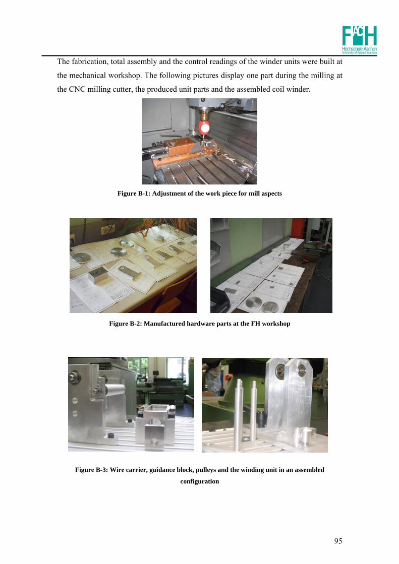
95
The fabrication, total assembly and the control readings of the winder units were built at
the mechanical workshop. The following pictures display one part during the milling at
the CNC milling cutter, the produced unit parts and the assembled coil winder.
Figure B-1: Adjustment of the work piece for mill aspects
Figure B-2: Manufactured hardware parts at the FH workshop
Figure B-3: Wire carrier, guidance block, pulleys and the winding unit in an assembled
configuration

96
Figure B-4: Assembled coil winder without pulleys and the coil mould

97
Appendix - C Coil Winder Circuit Design

98
Figure C-1: MCU circuit design

99
Figure C-2: Stepping motor circuit design

100
Figure C-3: Connector circuit design

101
Figure C-4: Power unit circuit design

102
Appendix - D Coil Winder Calibration Interface

103
The connection between the drive unit and the PC is established by pushing the
“connect” button at the user surface shown in the next figure 10-3.
Figure D-1: Connection surface
The communication port and the baud rate are actually automated adjusted, but it is
never a disadvantage to control the icons before the connection will be activated. The
guidance is driven with the user surface as follows:
Figure D-2: Guidance user surface
1
2

104
The red marked window number one is supposed to drive the stepping motor of the
winding unit. This section is actually able to drive the stepping motor in both rolling
directions, but because of safety reasons only the winding direction is activated. The
second section allows a very fine drive of the linear actuator of the guidance unit. The
particular direction of motion is adjustable with (the) two arrows, whereby the step size
of the motions is manually adjustable from one to 100 steps. For a proper guidance
calibration run the linear actuator must be to his absolute zero point which need to be
countersigned with pushing of the button “Lin=0”. The operation borders of the
guidance are adjusted manually by the turning points of the traverse paths of the
guidance unit. The lower reversal point must be tuned manually as a minimum value
which is set by pushing the button “Set Min” at the user surface. The second reversal
point can also be appointed manually but with the knowledge about the defined coil
width, allows the software the definition of the maximum value by entering the size of
the coil width which is displayed in figure 10-5. The minimum and maximum values
can be checked by using the “Move Min” and “Move Max” buttons.