DESIGN, CONSTRUCTION, AND VALIDATION OF THE AFIT

SMALL SCALE COMBUSTION FACILITY AND SECTIONAL MODEL OF THE ULTRA-COMPACT COMBUSTOR

THESIS

Wesly S. Anderson, Second Lieutenant, USAF

AFIT/GAE/ENY/07-M01

DEPARTMENT OF THE AIR FORCE AIR UNIVERSITY

AIR FORCE INSTITUTE OF TECHNOLOGY

Wright-Patterson Air Force Base, Ohio

APPROVED FOR PUBLIC RELEASE; DISTRIBUTION UNLIMITED

The views expressed in this thesis are those of the author and do not reflect the official policy or position of the United States Air Force, Department of Defense, or the United States Government.

AFIT/GAE/ENY/07-M01

DESIGN, CONSTRUCTION, AND VALIDATION OF THE AFIT SMALL SCALE COMBUSTION FACILITY AND SECTIONAL MODEL OF THE ULTRA-COMPACT

COMBUSTOR

THESIS

Presented to the Faculty

Department of Aeronautics and Astronautics

Graduate School of Engineering and Management

Air Force Institute of Technology

Air University

Air Education and Training Command

In Partial Fulfillment of the Requirements for the

Degree of Master of Science in Aeronautical Engineering

Wesly S. Anderson, BS

Second Lieutenant, USAF

March 2007

APPROVED FOR PUBLIC RELEASE; DISTRIBUTION UNLIMITED.

iv

AFIT/GAE/ENY/07-M01

Abstract The AFIT small-scale combustion facility is complete and its first experiment designed

and built. Beginning with the partially built facility, detailed designs have been

developed to complete the laboratory in order to run small-scale combustion experiments

at atmospheric pressure. A sectional model of the Ultra-Compact Combustor has also

been designed and built. Although the lab’s specific design intent was to study the

UCC’s cavity-vane interaction, facility flexibility has also been maintained for future

work. The design enabled the completion of liquid fuel and air delivery systems, power

and control systems, and test equipment. The design includes failsafe operation, remote

control, and adherence to SAE ARP 1256 testing standards. Construction of the

laboratory has forced design changes as new obstacles arose. As system construction has

been completed validation and troubleshooting have been undertaken. The AFIT facility

can now deliver air in two separately controlled air lines at up to 530 K (500 °F), at

delivery rates of 0.12 kg/s (200 SCFM) for the main line and 0.03 kg/s (60 SCFM) for the

secondary. A continuous dual syringe pump can deliver liquid fuel at up to 5.67 mL/s for

JP-8 equivalence ratios up to 4. Safe, remote ignition and shutdown are in place and all

test equipment fundamental to combustion is installed. The addition of an advanced laser

combustion diagnostics system adds more unique capability to the laboratory. The laser

system will provide instantaneous Raman and Raman spectroscopy, Coherent Anti-

Stokes Raman Scattering, Planar Laser-Induced Fluorescence, Laser-Induced

Incandescence and Planar Imaging Velocimetry diagnostic techniques.

v

Acknowledgements I would like to thank my wife for handling her first few years of marriage in a

new place and to a husband that is always working with such grace and show of support.

I want to thank my parents for raising me how they did. My brother and I won’t easily

forget their lessons of, “If you are gonna do something, do it right,” and a thousand

others.

I would like to thank my advisor, Major Richard Branam, for taking me on mid-

stride, providing direction and being so knowledgeable and approachable. I owe a thank

you to my first advisor, Dr. Ralph Anthenien for his foresight and expertise. I am very

thankful for Eric Dittman and his extra efforts on my behalf, and John Hixenbaugh for his

technical know-how, approachability, effort, and attitude.

Thank you to my friends for making things easier to bear. Special thanks to

Joshua Crouse, Tim Pitzer, Tim Booher, Erik Saladin and Barth Boyer for their extra

support. Also, I would like to thank Ryan Carr for always being up for some fun and a

run in the wildest places we could find in Ohio.

Finally, I owe everything to Jesus Christ, my refuge. It is all worthless apart from

you. Soli Deo Gloria.

Wesly S. Anderson

vi

Table of Contents

Page

Abstract .............................................................................................................................. iv

Acknowledgements............................................................................................................. v

Table of Contents............................................................................................................... vi

List of Figures .................................................................................................................. viii

List of Tables ..................................................................................................................... xi

List of Symbols ................................................................................................................. xii

List of Abbreviations ....................................................................................................... xiii

I. .........Introduction............................................................................................................. 1

1.1 Research and Design Perspective ............................................................... 1

1.2 Description of the Ultra Compact Combustor ............................................ 2

1.3 Objectives ................................................................................................... 4

1.4 Methods....................................................................................................... 5

II.........Theory and Background.......................................................................................... 7

2.1 History of UCC Research ........................................................................... 7

Standard Combustor Design ....................................................................... 7

Inter-Stage Turbine Burning ....................................................................... 8

Trapped Vortex Combustion..................................................................... 10

Centrifugally Loaded Combustion............................................................ 11

Experimental Research on the UCC ......................................................... 11

Computational Fluid Dynamics Research on the UCC ............................ 13

2.2 2-D Sector Rig Design .............................................................................. 14

2.3 Existing Experimental Facility and Intended Measurements ................... 16

Emissions measurements .......................................................................... 17

Mass Flow Measurement .......................................................................... 22

Pressure Transducers and Thermocouples................................................ 23

2.4 Laser Diagnostic Systems......................................................................... 23

Instantaneous Raman and Raman Spectroscopy....................................... 23

Page

vii

CARS ........................................................................................................ 29

PLIF .......................................................................................................... 32

LII ............................................................................................................. 39

PIV ............................................................................................................ 41

III........Methodology......................................................................................................... 44

3.1 System Design and Operation................................................................... 44

Computer Control and Data Acquisition .................................................. 45

Data Acquisition and Control Software.................................................... 47

Power supply systems ............................................................................... 49

Combustor Rig Air.................................................................................... 54

Fuel Supply ............................................................................................... 58

Remote Ignition ........................................................................................ 60

Nitrogen Purge .......................................................................................... 61

Gas Analyzer............................................................................................. 64

Emissions Collection ................................................................................ 65

Instrument Air........................................................................................... 68

Combustor Stand....................................................................................... 69

Exhaust System......................................................................................... 70

Laser Diagnostic System........................................................................... 71

3.2 Real Combustor Design ............................................................................ 72

IV. ......Results and Discussion ......................................................................................... 76

V.........Conclusions........................................................................................................... 79

5.1 Overview of Project .................................................................................. 79

5.2 Future Work and Recommendations ........................................................ 80

Appendix A: System Technical Information .................................................................... 82

Appendix B: Operational Checklist for System Startup.................................................. 94

Bibliography ..................................................................................................................... 96

viii

List of Figures

Page

Figure 1: Orginial UCC experimental setup without RVC’s. (Zelina, Sturgess and Shouse, 2004)..................................................................................................... 3

Figure 2: Detail of UCC with RVC’s, this model was used in CFD research. (Greenwood, 2005:1-4) ...................................................................................... 3

Figure 3: Detail of air and fuel injection in the UCC. (Anthenien et al, 2001:6) ............. 4

Figure 4: Standard combustor design (Wilson, 1998:528) ................................................. 8

Figure 5: Engine cycle for a typical gas turbine (dashed) and those with turbine burning included (solid). (Sirignano and Liu, 2000:9) ..................................... 8

Figure 6: The Trapped Vortex Combustion concept. (Greenwood, 2005:1-2)............... 10

Figure 7: Curved sectional 2-D rig used by Moenter for CFD comparisons of the final design. This plot shows contours of temperature (K). Airflow is to the right in the cavity and out of the page in the main vane. (Moenter, 2006: 112) ....................................................................................... 14

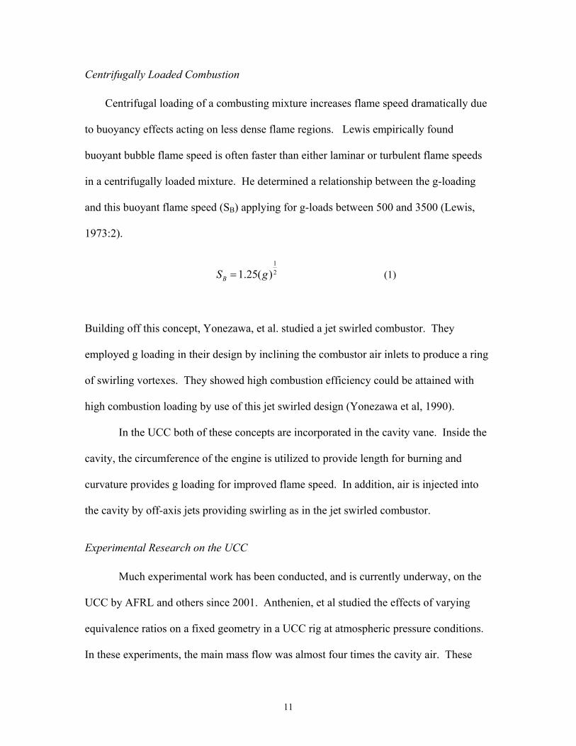
Figure 8: Comparison of the 2-D curved cavity rig used as the final curved 2-D sectional design (top) with the baseline configuration using boundary conditions to simulate a full 360 cavity (bottom). Cavity airflow is left to right in both cases; main airflow is out of the page. Velocity vectors are shown colored with temperature (K). The large eddy in the center of the field clearly shows the interaction of the RVC with the cavity flow. The large amount of air entrained into the room in the experimental rig is also shown. (Moenter 2006: 117)...................................... 16

Figure 9: Paramagnetic oxygen detector theory (Supplemental Oxygen Manual, Sec. 6:17-19) .................................................................................................... 19

Figure 10: Principle of operation of the paramagnetic oxygen detector (Supplemental Oxygen Manual, Sec. 6:17-19)................................................ 20

Figure 11: NDIR Analyzer for CO and CO2 (Manual for Infrared Analyzers, Sec 2: 9) .................................................................................................................. 21

Figure 12: Incoherent light scattering and resulting spectra. The upper diagram indicates two electronic energy states with vibrational energy levels. Upward arrows indicate increasing energy. Raman and Rayleigh scattering are shown. The symbol λ indicates signal wavelength. (Eckbreth, 1988:11).......................................................................................... 25

Figure 13: Basic setup for a time averaged Raman measurement. CCD cameras are commonly in use today in place of photomultipliers. (Eckbreth, 1988:190) ......................................................................................................... 29

Page

ix

Figure 14: Example of dual-pump CARS experimental setup for N2-CO2 measurements. OSC is oscillator, AMP is amplifier, NBDL is a narrowband dye laser, BBDL is a broadband dye laser and the SPEX 1000M is a 1.0m spectrometer. (Roy, Meyer, Lucht, et al, 2005:22, used with permission) ...................................................................................... 32

Figure 15: Fluorescent absorption, emission and resulting spectra. The upper diagram indicates two electronic energy states with vibrational energy levels. Upward arrows indicate increasing energy. The symbol λ indicates signal wavelength. (Eckbreth, 1988:11) ........................................... 34

Figure 16: Fluorescent absorption and emission spectra for the OH radical at 2000K and 1 atm in air. These plots were produced with the LIFBASE software. They show maximum absorption at nearly 283 nm and maximum emission at 309 nm. ........................................................................ 37

Figure 17: Schematic of experimental setup for conducting simultaneous LII and OH PLIF measurements. The OH PLIF is provided by the pumped dye laser at 284 nm. (Meyer and Roy, 26:2003, used with permission)................. 38

Figure 18: California Analytical Instruments raw exhaust analyzer test bench (l) and laboratory computer control station (r). .................................................... 44

Figure 19: Diagram of control systems connectivity........................................................ 45

Figure 20: Peripheral hardware what provides direct control of the laboratory systems by the CPU. ........................................................................................ 47

Figure 21: Combustion facility control software flow of operation. (Dittman, 2006:32) ........................................................................................................... 49

Figure 22: AC Power wiring diagram............................................................................... 51

Figure 23: DC power wiring diagram............................................................................... 52

Figure 24: Power distribution and signal lines in pressure transducer boxes. .................. 53

Figure 25: Rig airlines upstream of electric heaters. ........................................................ 54

Figure 26: Rig airflow control loop. ................................................................................. 55

Figure 27: Signal line connection schematic of rig air control loop and data transmission. .................................................................................................... 56

Figure 28: Heater emergency shutoff and data transmission............................................ 58

Figure 29: Liquid fuel pump and control system.............................................................. 59

Figure 30: ISCO fuel pump system. ................................................................................. 60

Figure 31: Solenoid valves controlling ignition and purge systems and their connection to the combustor stand................................................................... 61

Figure 32: Liquid and gas systems in the laboratory. ....................................................... 63

Page

x

Figure 33: Oil heated emissions probe and electrically heated line on test stand............. 66

Figure 34: Mokon heater and pump unit for heat transfer oil used to cool emissions probe................................................................................................ 67

Figure 35: Temperature control loop of exposed emissions line. ..................................... 68

Figure 36: Combustor stand with exhaust probe assembly. ............................................. 70

Figure 37: Flat combustor cavity design with main vane. Airflow direction is shown in red. .................................................................................................... 72

Figure 38: Cross-section of curved combustor cavity. Airflow is shown in red; fuel flow is shown in blue. The location of airflow through the main vane (moving into the page) and the radial vane cavity (RVC) is also indicated. .......................................................................................................... 73

xi

List of Tables

Page

Table 1: Fundamental vibrational frequencies of selected molecules of interest. The vibrational frequencies represent the Stokes shift of the incident light for Raman techniques. ............................................................................. 26

Table 2: Major allowed electronic transitions for species of interest . These transitions represent the bands active to fluorescent absorption. (Eckbreth, 1979:260-265) ................................................................................ 36

Table 3: Ranges for gases analyzed by CAI test bench. ................................................... 65

Table 4: Wiring code for NI SCXI 1100 DAQ measurement and control system. .......... 82

Table 5: Wiring code for Opto 22 PB24 solid state relay board used for control of systems throughout the room. .......................................................................... 85

Table 6: Wiring and digital channel code for Opto 22 G4PB24 optically isolated solid-state relay board used for controlling range selection on the raw emissions test bench......................................................................................... 86

Table 7: Type, concentration and connection for all laboratory gases. ............................ 87

Table 8: Compiled list of major equipment and technical data by system. ...................... 88

List of Symbols Symbol C2 Diatomic carbon

CH4 Methane

CO Carbon Monoxide

CO2 Carbon Dioxide

C2H2 Acetylene

C2H4 Ethylene

g Gravitational constant

h Water content

HC Heat of combustion of fuel

H2O Water

k Turbulent kinetic energy

M Molecular Mass

Na Sodium

N2 Nitrogen

NO Nitric Oxide

NOX Oxides of Nitrogen

NO2 Nitrogen Dioxide

OH Hydroxide

O2 Oxygen

SB Buoyant flame speed

X Molar fraction air to fuel

x Number of carbon atoms, undefined quantity

y Number of hydrogen atoms

Z Constituent Z

α Ratio of hydrogen to carbon atoms

ε Rate of turbulent kinetic energy dissipation

ηb Combustion efficiency %

xii

List of Abbreviations Abbreviation AC Alternating current

AFIT Air Force Institute of Technology

AFRL Air Force Research Laboratory

ARP Aerospace Recommended Practice

CAI California Analytical Insturments

CARS Coherent Anti-Stokes Raman Spectroscopy

CCD Charge coupled device

CFD Computational Fluid Dynamics

CPU Central Processing Unit

CTB Continuous turbine burner

DAQ Data acquisition

DC Direct current

EI Emissions Index

FID Flame ionization detector

HCLD Heated chemiluminescent detection

HID High image density

I/O Input/output

IGV Inlet guide vanes

ISSI Innovative Scientific Solutions Inc.

ITB Inter-stage turbine burner

LDV Laser Doppler Velocimetry

LID Low image density

LII Laser-Induced Incandescence

LSV Laser speckle Velocimetry

mA milli-Amps

NDIR Non-dispersive infrared

Nd:YAG Neodymium-doped yttrium aluminium garnet

NI National Instruments

xiii

nm nanometer

PAH Polycylic aromatic hydrocarbons

PC Personal computer

PID Proportional-integral-derivative

PIV Particle Imaging Velocimetry

PLIF Planar Laser Induced Fluorescence

ppm Parts per million

PRV Pressure reducing valve

RNG Renormalization group theory

RVC Radial Vane Cavity

SAE Society of Automotive Engineers

SCFM Standard cubic feet per minute

SCXI Signal Conditioning Extension for Instrumentation

SSR Solid state relay

ST Specific thrust

TSFC Thrust specific fuel consumption

TVC Trapped Vortex Combustion

UCC Ultra Compact Combustor

USB Universal Serial Bus

VAC Volts alternating current

VDC Volts direct current

VI Virtual Instrument

2-D Two dimensional

3-D Three dimensional

xiv

DESIGN, CONSTRUCTION, AND VALIDATION OF THE AFIT SMALL SCALE COMBUSTION FACILITY AND SECTIONAL MODEL OF THE ULTRA-

COMPACT COMBUSTOR

I. Introduction

1.1 Research and Design Perspective

Efficient use of energy has always been highly desirable and this is true more today

than ever. The cost of energy in terms of economic and environmental impact is being

felt more and more as the world’s demand increases. The Department of Defense

requires enormous amounts of fuel for all of its endeavors. The vast majority of this goes

to air operations. Increasing demand for energy from the Air Force and the world is not

going away anytime soon, so better technology is the best and only answer to this

problem. In the case of aircraft operations, improvements in turbine engine cycle

performance can provide significant steps in the right direction.

The Ultra Compact Combustor (UCC) may be a partial solution for this problem. By

making significant changes in airflow direction and fuel mixing in the combustor, the

UCC will greatly reduce the axial length required for efficient combustion in a gas-

turbine engine. This has the potential for two major advantages: First, advanced engine

concepts such as inter-stage turbine burners (ITB) to improve thermodynamic cycle

efficiencies may be utilized. Secondly, the UCC may be used as a standard combustor

positioned between the compressor and turbine, reducing the weight and length of the

engine. (Anthenien et al, 2001)

Previous experiments and Computational Fluid Dynamics (CFD) studies have been

conducted on variations of the UCC design with promising results. However, due to

geometry constraints no one has been able to directly study the flow field and combustion

1

inside much of the UCC. In order to do this it was necessary to build a sectional model

and find an associated laboratory facility to provide the necessary diagnostics. It was

determined that a new testing facility at the Air Force Institute of Technology (AFIT)

would be constructed to investigate the cavity-vane interactions of the UCC sectional

models and provide future combustion test capability for AFIT.

1.2 Description of the Ultra Compact Combustor

The full UCC (shown in Figure 2) is a product of research at the US Air Force

Research Laboratory (AFRL), Propulsion Directorate at Wright-Patterson Air Force Base

in Dayton, Ohio. Inspiration for the combustor came from a paper written by researchers

at the University of California, Irvine demonstrating the use of inter-stage turbine burners

(ITB) to significantly improve major engine performance measurements.

The combustor consists of an annular main flow around a blunt body positioned

along the axial direction. A cavity surrounds this body running circumferentially around

the main flow as shown in Figure 1. The cavity provides the main mixing and

combustion region. The air-fuel mixture travels around this cavity providing necessary

residence time for combustion without significant axial length. Air is injected into the

cavity through 24 jets in the outer wall of the cavity. These jets are angled away from

radial direction to provide swirling as shown in Figure 3. This jet swirling, along with

the circumferential motion of the mixture through the cavity vane increases the flame

speed. Fuel injects through an atomizer into six recessed chambers, utilizing trapped

vortex combustion (TVC) to stabilize the flame and improve combustion efficiency.

The cavity vane is open to the axial main flow of air through the combustor. Six

evenly spaced, radially extending airfoils hold the annular blunt body in place. These

2

airfoils also simulate inlet guide vanes (IGV) or stator blades, envisioning the use of the

UCC as an ITB in the future. In order to provide for mass transport from the cavity flow

to the main flow, radial vane cavities (RVC) are cut into the airfoil blades. This creates

an intermediate combustion zone and provides a pressure gradient, drawing mass from

the cavity vane into the main vane flow stream. A shown in Figure 3 the six fuel

injection points are located directly over the RVC’s and the 24 air injection jets are

evenly spaced between the fuel injectors.

Figure 1: Orginial UCC experimental setup without RVC’s. (Zelina, Sturgess and Shouse, 2004)

Fuel

Cavity Air Jets

Main Airflow

Vanes

Fuel

Cavity Air Jets

Main Airflow

Vanes

RVC

Figure 2: Detail of UCC with RVC’s, this model was used in CFD research. (Greenwood, 2005:1-4)

3

CenterBody

Annulus (MainAir Flow)

CavityFuel

Air Jets

Figure 3: Detail of air and fuel injection in the UCC. (Anthenien et al, 2001:6)

1.3 Objectives

Construction of the AFIT small-scale combustion facility began in 2005 in building

641 room 258 under the direction of Dr. Ralph Anthenien and the efforts of Lt. Eric

Dittman. At the completion of Lt. Dittman’s work most of the major components of the

facility were selected and in place. Also, a general plan for the integration of these

components into a system had been developed, and much construction had been

undertaken.

The facility was primarily intended to study the UCC cavity-vane interaction.

However, as AFIT’s first combustion facility it would also need to be expandable for

future experiments. Safe, centralized control of the process through a computer station

increases manageability of such a complex and potentially dangerous system. This

station also allows for automated recording of data for accuracy and repeatability.

Emissions analysis provides valuable information by using a gas analyzer and samples

taken from the test section. Liquid fuel and heated air are provided in a controlled

manner producing equivalence ratios between 0.2 and 4 at flows of 0.1 to 0.3 Mach at

4

low pressures in the test section (Dittman, 2006: 2). Safety systems allow safe operation

to be observed at all times. Finally, ready access for laser diagnostics is provided by the

final installation of a laser diagnostics system.

At the beginning of the author’s work, many of the specific details of the facility

design were undetermined, and much construction still needed to be accomplished, along

with an overall evaluation of the systems functionality. Also, calibration, operational

procedures and repair documentation needed to be developed. Finally, a sectional UCC

rig needed to be designed and built to provide the facility with its first experiment and

fulfill its original intent.

1.4 Methods

To complete the facility and accomplish all the previous goals several steps were

undertaken:

1) Study of existing project objectives and design. It was necessary to understand

the full intent of the project and the intent of the original facility design in order to begin

the completion of the facility. A good working knowledge of the particular pieces was

also necessary. In addition, previous CFD studies and work on the UCC needed to be

well understood in order to work on the sectional UCC rigs.

2) Assessment of project progress, system by system. To develop a to-do list the

project’s actual progress needed to be understood in detail. For example, approximately

half of the signal wiring from various instruments had been run to the computer station.

It thus became necessary to know what particular signals were necessary and still needed

to be constructed. Similar scenarios existed in many of the sub-systems.

5

3) Design or re-design of systems. Although general plans were often in place,

specifics of a system design or its integration often were not. Detailed questions needed

answering, such as: what type of valve would work best, or what materials are compatible

with a particular gas? Also, the addition of systems with no existing plans made it

necessary to begin new designs from the ground up.

4) Purchase of necessary parts to complete design. Selection and purchase of

parts was a major effort of this project. This was often concurrent with the final design of

the system as most of the pieces for the design were off-the-shelf.

5) Construction and troubleshooting. Construction often provided its own unique

challenges, forcing on-the-spot redesign and creative solutions. This project has re-

enforced the lesson that “the devil is in the details” as many design and construction

challenges remained even with a good plan and major infrastructure in place.

6

II. Theory and Background

2.1 History of UCC Research

Standard Combustor Design

A standard combustor in most modern gas turbines uses some variation of the

combustor can, or flame tube, concept. As seen in Figure 4 this type of combustor uses

fuel injection along the axial direction of the engine in the center of the combustion can.

Air enters the can from the compressor through turning vanes positioned around the fuel

injection point or multiple holes in the can’s side. Air entry is in two zones. A primary

zone provides near stoichiometric air for combustion and forces flow patterns for mixing.

The secondary (dilution) zone adds the remaining air to the mixture, cooling the gas and

providing an even temperature profile so it can safely enter the turbine (Wilson, 1998:

528). This standard combustor design relies almost entirely on axial length to provide

residence time for combustion. It causes significant pressure loss, as the axial flow must

decelerate for combustion to occur. It is also fixed in-between the compressor and

turbine of an engine and it thus limits possible variations of the engine’s thermodynamic

cycle.

7

Film-Cooling Air

Fuel In Fuel Injector

Primary Air Secondary or Dilution Air

From Compressor Diffuser or Heat Exchanger

Swirl Flow

Flame Tube

Primary Zone Secondary Dilution Zone

Recirculation Flow

Figure 4: Standard combustor design (Wilson, 1998:528)

Inter-Stage Turbine Burning

In 1999 Sirignano and Liu proposed a concept that would significantly improve the

efficiency of this gas turbine engine cycle. Figure 5 shows the T-S diagram for the major

types of cycles studied.

Figure 5: Engine cycle for a typical gas turbine (dashed) and those with turbine burning included (solid). (Sirignano and Liu, 2000:9)

S

T 03

T06

04 05

06 06’

07’

07

05

Qb

QtbQab

T04

Inlet

8

As one can see, addition of heat in the turbine can add a considerable amount of

energy to the cycle while remaining under the critical temperature limits of the turbine

blades. Using this concept on many types of gas turbine cycles, Sirgnano and Liu found

that use of a continuous turbine burner (CTB) would improve both the major engine

performance parameters: Specific thrust (ST) would increase dramatically with only

slight increases in thrust specific fuel consumption (TSFC). Using a CTB model, they

report an improvement in ST of up to 50% with little or no change in TSFC on a turbofan

engine (Sirignano and Liu, 1999:8). However, early in their paper the researchers admit

the i r

r,

er

,

savings. If used

as a

nherent difficulty of burning in a rotor stage of the turbine, and instead focus thei

efforts on the more practical use of inter-stage turbine burners (ITB’s). These ITB’s

would ideally burn in the stator stages throughout the turbine. This design provides a

more practical way to approach the desirable performance of the CTB.

The advantages of an ITB engine over a conventional design are obvious; howeve

stator burning is still a very difficult proposition. The most significant issue is the large

axial length necessary in a standard combustor to provide for adequate residence time to

efficiently mix and burn fuel. This is many times longer than the typical stator stage.

The Ultra Compact Combustor (UCC) provides a solution to the problem of

residence time in a stator. The literature states that this combustor may be used as eith

a standard burner at the inlet guide vanes (IGV) of the turbine or an ITB. In either case

it would reduce the length of the engine significantly, resulting in weight

n ITB it would significantly improve the cycle efficiency.

9

The UCC uses two major combustion concepts in an effort to burn fuel efficiently

over a short axial length: Trapped vortex combustion (TVC) and use of centrifugal-force

effe

Trapped Vortex Combustion

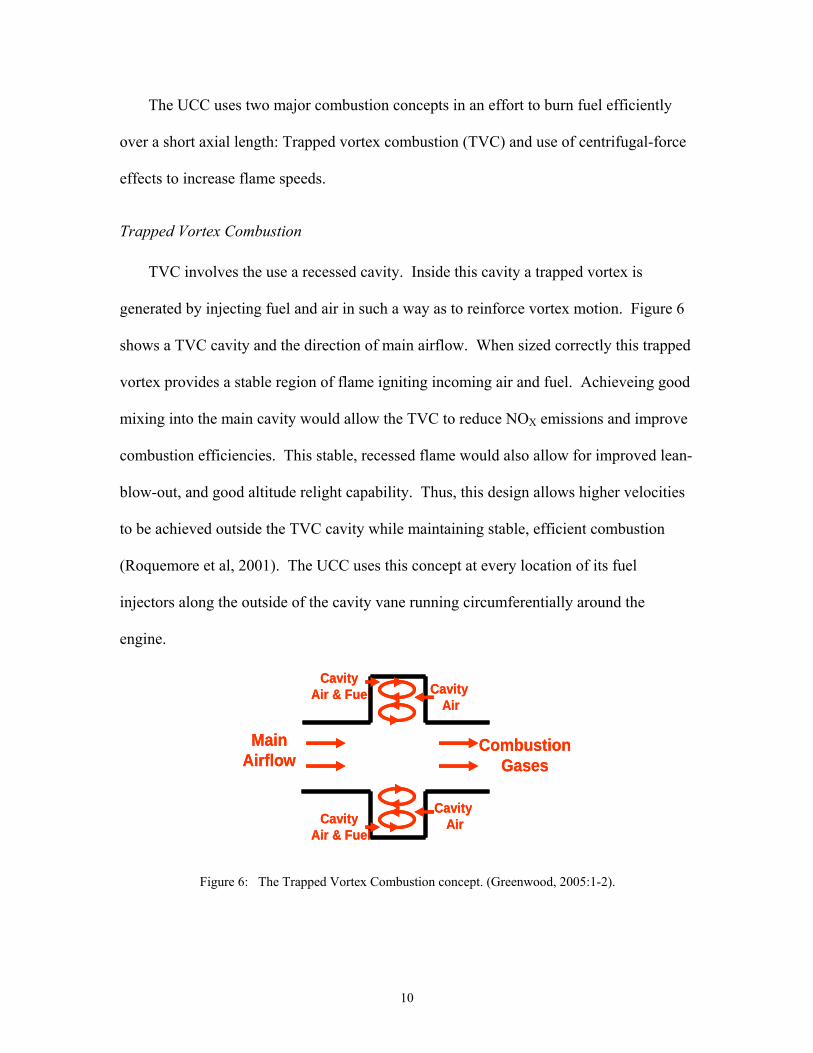
TVC involves the use a recessed cavity. Inside this cavity a trapped vortex is

generated by injecting fuel and air in such a way as to reinforce vortex motion. Figure 6

shows a TVC cavity and the direction of main airflow. When sized correctly this trapped

vortex provides a stable region of flame igniting incoming air and fuel. Achieveing good

mixing into the main cavity would allow the TVC to reduce NOX emissions and improve

combustion efficiencies. This stable, recessed flame would also allow for improved lean-

light capability. Thus, this design allows higher velocities

to b n

cts to increase flame speeds.

blow-out, and good altitude re

e achieved outside the TVC cavity while maintaining stable, efficient combustio

(Roquemore et al, 2001). The UCC uses this concept at every location of its fuel

injectors along the outside of the cavity vane running circumferentially around the

engine.

Main Airflow

Cavity Air & Fuel

CombustionGases

Cavity Air

Cavity AirCavity

Air & Fuel

Main Airflow

Cavity Air & Fuel

CombustionGases

Cavity Air

Cavity AirCavity

Air & Fuel

Figure 6: The Trapped Vortex Combustion concept. (Greenwood, 2005:1-2).

10

Centrifugally Loaded Combust

Centrifugal loading of a combusting mixture increases flame speed dramatically due

to buoyancy effects acting on less dense flame regions. ally found

buoyant bubble flame speed is often faster than either laminar or turbulent flame speeds

in a centrifugally loaded mixt termined a relationship between the g-loading

and this buoyant flame speed (SB) applying for g-loads between 500 and 3500 (Lewis,

1973:2).

g

ustion loading by use of this jet swirled design (Yonezawa et al, 1990).

In the UCC both of these concepts are incorporated in the cavity vane. Inside the

cavity, the circumference of the engine is utilized to provide length for burning and

urvature provides g loading for improved flame speed. In addition, air is injected into

Experimental Research on the UCC

Much experimental work has been conducted, and is currently underway, on the

UCC by AFRL and others since 2001. Anthenien, et al studied the effects of varying

equivalence ratios on a fixed geometry in a UCC rig at atmospheric pressure conditions.

In these experiments, the main mass flow was almost four times the cavity air. These

ion

Lewis empiric

ure. He de

Building off this concept, Yonezawa, et al. studied a jet swirled combustor. They

employed g loading in their design by inclining the combustor air inlets to produce a rin

of swirling vortexes. They showed high combustion efficiency could be attained with

high comb

121.25( )BS g= (1)

c

the cavity by off-axis jets providing swirling as in the jet swirled combustor.

11

experiments used JP-8 and ethanol fuels over a large range of operating conditions.

Significantly shorter flame lengths were observed as compared to a standard, swirl

stabilized combustor. High efficiencies of +99% were achieved up to cavity equivalence

ratios greater than 2 and lean blowout was found down to a cavity equivalence ratio of

0.5 (Anthenien et al, 2001).

Zelina et al in 2001 also conducted studies into the effect of fuel injection method

and angle. They found fuel injector type and angle greatly affected the UCC’s

combustion efficiency. From the data, they proposed two modes of operation. For low

loadings, the flame seemed to be injector-stabilized. At higher loadings, the flame was

bulk-flow stabilized. They found the combustor had stable and efficient operation with

little pressure drop (2%). Finally, they noted increased g loading improved combustion

efficiency by creating high radial turbulence in the cavity. (Zelina, et al, 2001)

Laser Doppler Velocimeter (LDV) experiments on the UCC found

circumferential velocities of 20-45 m/s with accelerations of 1000-4000g in the cavity.

Quaale et al compared these results to CFD models and found good agreement. These

experiments found the cavity velocities were insensitive to the main flow velocity.

Again, combustion efficiencies increased with g-loading, while residence time decreased.

This increase in g loading also increased the CO Emission Index (Quaale et al, 2003).

Higher pressure rigs (Zelina, Shouse, and Neuroth, 2005) and the incorporation of

the RVC (Radial Vane Cavity) (Zelina, Sturgess, and Shouse, 2004) were also introduced

in several other experiments. These continued to show promise as the UCC performed

well. Work continues today with the introduction of changes based on previous

experiments and CFD research.

12

Computational Fluid Dynamics Research on the UCC

AFRL researchers and previous AFIT students have also conducted

c tational fluid dynamics (CFD) studies to examine the mixing and combustion

inside the UCC. The AFIT work was begun by Greenwood using the commercial

software FLUENT and standard k-ε turbulence models with second order, implicit

solvers for steady state solutions. Greenwood first developed the proper heat tran

fuel injection models and made a

ompu

sfer and

comparison of a one-sixth sector model of the

changes in the geometry of the cavity (Greenwood, 2005). Anisko continued this work

by improving periodic boundaries to include fuel particles, and investigations of further

geometric variations (Anisko, 2006).

Moenter built on this work but used a model based on a statistical technique

known as renormalization group theory (RNG). This RNG k-ε model was intended to

provide greater accuracy and reliability than previous models. Moenter also corrected

some mistakes from previous research. Notably he found pressure boundary conditions

used incorrectly in Greenwood and Anisko’s work. He then evaluated several numerical

models at three cases of pressure and mass flow rates to develop both a 2-D flat and

curved cavity rig expected to closely behave like the entire UCC in a one-sixth (60°)

model. He soon found that a larger section of one-third (120°) was necessary. The

combustor’s behavior was compared to experiment based on the examination of velocity,

temperature and other properties of the flow field at pre-defined locations to give a

quantitative measurement. Also, measurements such as efficiency, emissions,

combustor to experimental data from AFRL for the full UCC rig. He also studied

13

temperature distribution and pressure loss across the combustor were used as a qualit

basis of comparison (Moenter, 2006).

ative

RVC

2.2 2-D Sector Rig Design

The purpose of these new sector rig CFD models created by Moenter was to

design real experimental 2-D flow rigs allowing greater optical access to study flow

patterns and combustion in the UCC. Also, the creation of both a flat and curved cavity

combu

ombustor’s performance.

mined the flow behavior of the RVC and its wake were

of inter o

ter

Figure 7: Curved sectional 2-D rig used by Moenter for CFD comparisons of the final design. This plot shows contours of temperature (K). Airflow is to the righ of the page in the main vane. (Moenter, 2006: 112)

t in the cavity and out

stor would allow for empirical study into the effect of centrifugal loading on the

c

Specifically, it was deter

est and no good access could be gained with existing full (360°) UCC rigs. T

simulate this cavity-vane interaction on a sectional rig allowing optical access, Moen

14

found the most important areas to be reproduced were of the circumferential flow over

the axial vane (representing a stator vane) and the main flow approaching this area.

a

eful

optical

l

Extra mass flow into the cavity was necessary in order to properly account for the

mass entrained in the full combustor. As Figure 7 shows, two 60° segments, each with

fuel injection point, were deemed necessary to provide similar combustion behavior at

the RVC. Additional air inlets at the cavity start provided the proper local equivalence

ratio at the first fuel injection point. The main flow cavity was squared to provide us

access to the RVC. The design was then simplified by imbedding half the axial

vane in a side wall not used for viewing and adjusting the geometry of the rig accordingly

(Moenter, 2006:36). The size of the design was also reduced to one-sixth of the origina

UCC in order to match airflow capabilities of the experimental facility (Dittman, 2006:

17).

15

Figure 8: Comparison of the 2-D curved cavity rig used as the final curved 2-D sectional design (top) with the baseline configuration using boundary conditions to simulate a full 360 cavity (bottom). Cavity airflow is left to right in both cases; main airflow is out of the page. Velocity vectors are shown colored with temperature (K). The large eddy in the center of the field clearly shows the interaction of the RVC with the cavity flow. The large amount of air entrained into the room in the experimental rig is also shown. (Moenter 2006: 117)

2.3 Existing Experimental Facility and Intended Measurements

In order to generate useful information from any combustion experiment

performed on the UCC it is necessary to measure several quantities considered

fundamental to any combustion test facility. With the addition of laser diagnostics, the

16

facility can take necessary measurements on the UCC 2-D sectional rig as proposed.

Thus, the facility can also provide more advanced experiments for any suitable

combustion device. This section will examine these measurement techniques.

Emissions measurements

One of the fundamental quantities of interest is the emissions index (EI) of major

combustion products. In general the emissions index (as defined in SAE ARP 1533:

Section A1) is as follows:

Moles of Pollutant Molecular Weight of Pollutant* *(1000)Moles of Fuel Molecular Weight of FuelxEI = (2)

The emissions index is useful in calculating the efficiency of the combustor.

Combustion efficiency gives an indication of how well the energy contained in fuel

converts into heat addition to the air traveling through the combustor. According to the

SAE standards, this can be calculated by the following:

1.00 4.346 (100)1000

x yC HCOb

C

EIEIH

η⎡ ⎤

= − −⎢⎢ ⎥⎣ ⎦

⎥ (3)

Where HC is the heat of combustion of the fuel and ηb is the efficiency in percent. EICO

and EICxHy are defined as:

[ ][ ] [ ]

[3

2

10 1 ( / )COCO

C Hx y

CO MEI T X mM MCO CO C H α

= ++⎡ ⎤+ + ⎣ ⎦

] (4)

17

[ ] [ ][

3

2

101 ( / )x y

x y

C Hx yC H

C Hx y

MC HEI T X m

M MCO CO C H α

⎡ ⎤⎣ ⎦= ++⎡ ⎤+ + ⎣ ⎦

] (5)

Here [ ] indicates the concentration of the molecule enclosed. M represents the

molecular weight and α is the ratio y/x. T is the molecular fraction of carbon dioxide in

air. Its value is assumed to be 0.00034. X/m is defined as:

[ ] 2/4(1 / 2)

ZX mh TZ

α−=

+ − (6)

Where X is the molar fraction of air to fuel. The value h is the water content of

the inlet air. Also, Z is defined as:

[ ] [ ]

[ ] [ ]2

2

222 x y

x y

yCO C H NOx xZ

CO CO C H

⎛ ⎞ ⎡ ⎤− − − +⎜ ⎟ ⎣ ⎦⎝ ⎠=⎡ ⎤+ + ⎣ ⎦

(7)

The AFIT facility uses a probe to capture emissions from a combustion device

such as the UCC. Gases entering the probe are then pumped to several sensors,

combined into a single gas analyzer unit. The sensors in the unit are used to measure the

concentrations of important combustion products and thus calculate the Emissions Index

of that product. The gas analyzer measures total hydrocarbons, nitric oxide, carbon

monoxide, carbon dioxide and oxygen concentrations in emission gases and meets SAE

ARP 1256 standards for accuracy (Dittman, 2006:24).

18

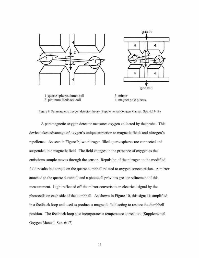
1 quartz spheres dumb-bell 3 mirror 2 platinum feedback coil 4 magnet pole pieces

Figure 9: Paramagnetic oxygen detector theory (Supplemental Oxygen Manual, Sec. 6:17-19)

A paramagnetic oxygen detector measures oxygen collected by the probe. This

device takes advantage of oxygen’s unique attraction to magnetic fields and nitrogen’s

repellence. As seen in Figure 9, two nitrogen filled quartz spheres are connected and

suspended in a magnetic field. The field changes in the presence of oxygen as the

emissions sample moves through the sensor. Repulsion of the nitrogen to the modified

field results in a torque on the quartz dumbbell related to oxygen concentration. A mirror

attached to the quartz dumbbell and a photocell provides greater refinement of this

measurement. Light reflected off the mirror converts to an electrical signal by the

photocells on each side of the dumbbell. As shown in Figure 10, this signal is amplified

in a feedback loop and used to produce a magnetic field acting to restore the dumbbell

position. The feedback loop also incorporates a temperature correction. (Supplemental

Oxygen Manual, Sec. 6:17)

19

1 measuring cell 4 feedback amplifier 2 “led” light beam 5 output amplifier 3 photo cell 6 meter indication

Figure 10: Principle of operation of the paramagnetic oxygen detector (Supplemental Oxygen Manual, Sec. 6:17-19) A Non-Dispersive Infrared (NDIR) sensor measures carbon monoxide and carbon

dioxide. As shown in Figure 11 the sample gas is exposed in a circulating sample cell to

infrared light modulating at a regular frequency by a chopper blade. The detector then

absorbs residual light. The detector consists of pure CO or pure CO2 in two chambers.

Absorption of differing amounts of energy from the infrared light by the gas in the

detector causes a pressure difference across the two chambers; this is measured by a

micro flow sensor. This pressure difference relates to the amount of carbon monoxide

present in the sample. (Operation and Maintenance Manual for Infrared Analyzers, Sec

2: 9-10)

20

Infrared Source Infrared Source Unit

Chopper Motor

Chopper Blade

Sample Cell Micro-Flow Sensor

Detector

Rear Chamber Front Chamber

Sample In Exhaust

Figure 11: NDIR Analyzer for CO and CO2 (Manual for Infrared Analyzers, Sec 2: 9)

A heated chemiluminescent detection (HCLD) sensor measures oxides of

nitrogen. This sensor has two modes. In the NO mode, it first converts all NO to NO2 by

oxidation with molecular ozone derived from cylinder air. This reaction causes 10 to 15

percent of the NO2 molecules to be raised to an excited state and then emit photons. A

photodiode detector collects these photons and generates a DC current proportional to the

NO contained in the sample gas. This signal is amplified and sent to readouts and

outputs. In the NOX mode, the sensor first uses a NOX converter to reduce all NO2 to NO

and then repeats the same procedure as above. (Model 400 HCLD Instruction Manual:

23)

A flame ionization detector (FID) determines total Hydrocarbons (THC). This

sensor uses a hydrogen/helium burner sustained with carbon free cylinder air. When

sample gases pass through the flame, an ionization process produces electrons and

positive ions from any hydrocarbons present. A polarized electrode ring then collects the

21

ions and produces a low current. This current is proportional to the carbon content of the

sample gas. The sample is maintained at an elevated temperature for this process.

(Heated Hydrocarbon Analyzer Instruction Manual:26)

Mass Flow Measurement

Another fundamental quantity for combustion experimentation is equivalence

ratio. This is the ratio of the mass of fuel to the mass of oxidizer in the combustion

process. With enough information given it can describe a local region, parts of the

combustor, or the entire process. Usually of interest is the variation of emissions

products with equivalence ratio. In order to know this value the mass flow rate of both

the oxidizer and the fuel must be known.

Thermal mass flow meters measure the flow rate of air into the combustor in the

AFIT facility. The device measures airflow by two electronically heated elements. The

first element is isolated away from the flow; the second is placed in the air stream. When

convective heat transfer with the air cools the exposed element, more energy is sent to the

element to maintain the same temperature as the isolated element. This energy difference

between the two elements is proportional to the mass flow rate. (Fox Thermal

Instruments, Rev. E:1)

Finely controlled syringe pumps control the fuel flow directly. Thus, the user

determines the flow rate directly from supplied equipment. Therefore, the fuel flow rate

is also a known quantity.

22

Pressure Transducers and Thermocouples

To establish the thermodynamic state of the air and fuel entering the combustor

and for determining losses across the combustor both pressure and temperature are

measured at several locations. Pressure is measured by the use of pressure transducers.

These devices use deflection of a small diaphragm measured by strain gauges and related

to pressure. This signal is amplified and transmitted to an output. Temperature is

measured by thermocouples. These consist of two dissimilar metals brazed together at a

point. The connection generates a small voltage between the two metals proportional to

the temperature of the brazed point.

2.4 Laser Diagnostic Systems

The AFIT combustion facility includes the capability of remote combustion

diagnostics using optical techniques. This system uses a double pulsed neodymium-

doped yttrium aluminium garnet or Nd:YAG laser with associated equipment to provide

six diagnostic techniques useful for combustion phenomena. This includes instantaneous

Raman, Particle Image Velocimetry (PIV), Laser Induced Incandescence (LII), Planar

Laser-Induced Fluorescence (PLIF), Coherent Anti-Stokes Raman Scattering (CARS)

and Raman Spectroscopy. Each one of these techniques provides useful information

from the combustor in addition to the data generated from the gas analyzer,

thermocouples and pressure transducers.

Instantaneous Raman and Raman Spectroscopy

Instantaneous Raman or spontaneous Raman scattering is a method of scattering

laser light off matter to determine its composition. The process is known as

instantaneous because the laser energy is returned and collected at a rate faster than the

23

Kolmogorov characteristic time scale of the flow. Therefore, the measurement is made

before the flow field under study has time to change. Most commonly, a single laser in

the visible wavelength (400 to 700 nm) is used as a monochromatic source of radiation.

Scattering is a momentum interaction between photons. Visible wavelengths are

generally used for scattering processes as the strength of the scattered signal scales to the

fourth power of the incident wavelength. When this laser light hits matter, Raman,

Rayleigh, and Mie scattering occur simultaneously. Rayleigh and Mie scattering consist

of elastic exchanges of momentum between photons and different sizes of particles.

Rayleigh scattering is when the particle diameter is much less than the wavelength of the

incident light, Mie scattering is when larger particles interact with the incident beam. In

these cases, there is no change in the frequency of the light as no energy is exchanged

with the particles.

Raman scattering is an inelastic scattering of light by the particles of interest. As

the term inelastic implies, energy is exchanged with the molecules struck. Depending on

the nature of the interaction, the scattering is described as rotational, vibrational, or

electronic. Rotational Raman refers to the part of the process where no change in the

vibrational quantum number is observed. Otherwise, the process is known as vibrational-

rotational or vibrational Raman. Vibrational Raman bands are commonly the most useful

for diagnostic use. The returned Raman signal is incoherent, or un-laser like, in nature.

The process is often called spontaneous as the interaction is extremely fast compared to

other methods, on the order of 10-12 seconds or less (Eckbreth, 1988: 12). Due to the

exchange of energy between molecule and light, the Raman signal shifts in frequency

from the incident source. When energy transfers from the photon to the molecule, the

24

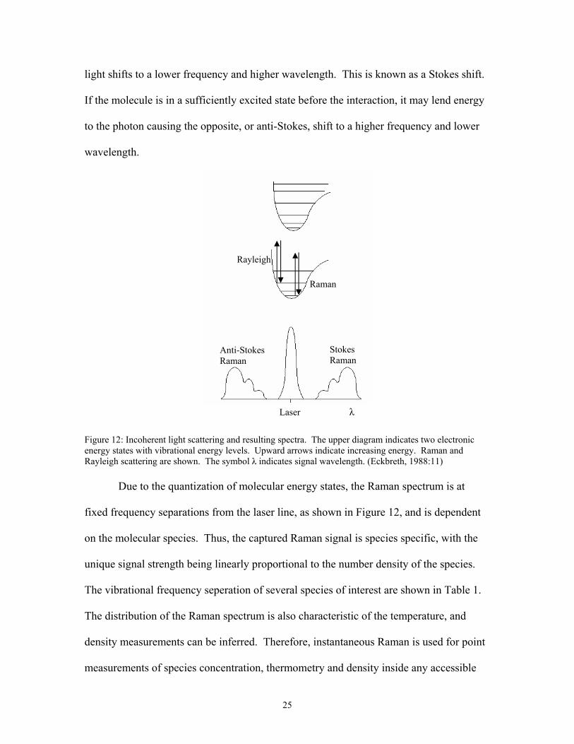
light shifts to a lower frequency and higher wavelength. This is known as a Stokes shift.

If the molecule is in a sufficiently excited state before the interaction, it may lend energy

to the photon causing the opposite, or anti-Stokes, shift to a higher frequency and lower

wavelength.

Rayleigh

Raman

Laser λ

Stokes Raman

Anti-Stokes Raman

Figure 12: Incoherent light scattering and resulting spectra. The upper diagram indicates two electronic energy states with vibrational energy levels. Upward arrows indicate increasing energy. Raman and Rayleigh scattering are shown. The symbol λ indicates signal wavelength. (Eckbreth, 1988:11)

Due to the quantization of molecular energy states, the Raman spectrum is at

fixed frequency separations from the laser line, as shown in Figure 12, and is dependent

on the molecular species. Thus, the captured Raman signal is species specific, with the

unique signal strength being linearly proportional to the number density of the species.

The vibrational frequency seperation of several species of interest are shown in Table 1.

The distribution of the Raman spectrum is also characteristic of the temperature, and

density measurements can be inferred. Therefore, instantaneous Raman is used for point

measurements of species concentration, thermometry and density inside any accessible

25

part of a combustion device. Like most laser diagnostic techniques, it is considered non-

intrusive, although the addition of energy to the flow field of interest by the laser does

have a small effect.

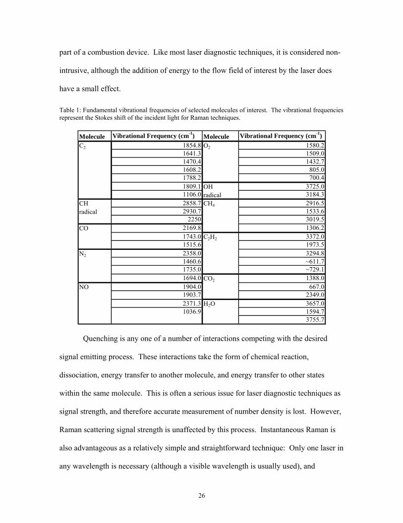
Table 1: Fundamental vibrational frequencies of selected molecules of interest. The vibrational frequencies represent the Stokes shift of the incident light for Raman techniques.

Molecule Vibrational Frequency (cm-1) Molecule Vibrational Frequency (cm-1)1854.8 1580.21641.3 1509.01470.4 1432.71608.2 805.01788.2 700.41809.1 3725.01106.0 3184.32858.7 2916.52930.7 1533.6

2250 3019.52169.8 1306.21743.0 3372.01515.6 1973.52358.0 3294.81460.6 ~611.71735.0 ~729.11694.0 1388.01904.0 667.01903.7 2349.02371.3 3657.01036.9 1594.7

3755.7

CH radical

CO

C2

NO

O2

N2

OH radicalCH4

H2O

C2H2

CO2

Quenching is any one of a number of interactions competing with the desired

signal emitting process. These interactions take the form of chemical reaction,

dissociation, energy transfer to another molecule, and energy transfer to other states

within the same molecule. This is often a serious issue for laser diagnostic techniques as

signal strength, and therefore accurate measurement of number density is lost. However,

Raman scattering signal strength is unaffected by this process. Instantaneous Raman is

also advantageous as a relatively simple and straightforward technique: Only one laser in

any wavelength is necessary (although a visible wavelength is usually used), and

26

collection of the signal does not require through optical access to the region of interest.

Calibration requires only the use of nitrogen for comparison. It also has the capability to

monitor several species simultaneously, with the same laser. In fact, the same process is

used to analyze solids, liquids or gases. In addition, resonant frequency enhancement can

increase the signal up to six orders of magnitude if the laser is tuned to be near the

resonant frequency of the molecule of interest (Eckbreth, 1988: 13). Spectral

interferences between the vibrational Raman bands of different gas types are rare, leading

to easy distinction of species. The cleanliness of these Raman spectra is also well suited

to thermometry.

However, Raman is generally considered problematic for studying much practical

combustion phenomena. This is mostly because the scattered signal is very weak with

cross sections around 10-31 cm2/steradian. This results in a collected Raman to laser

energy ratio in flames of 10-14 (Eckbreth, Bonczyk and Verdieck, 1979: 253). Also,

although Raman signals do not attenuate in clean flames, they are affected greatly by

particulates. This can result in high uncertainty of measurements as uncertainty is

directly linked to flow cleanliness and signal to noise ratios. Thus, in uncontrolled

environments, instantaneous Raman is plagued by low signal to interference ratios,

making it difficult to use in unclean flames of practical interest. To compensate,

relatively high incident beam energy must be used. Also, resonant enhancement can

boost signal strength, but for molecules of interest in combustion this is often in exotic

frequencies. Thus, it is not possible to perform such signal enhancement on many species

with common laser systems.

27

There are a large variety of experimental setups and techniques based on the

concept of Raman scattering. In fact, most of the laser diagnostics for combustion use

similar equipment. Historically, typical Raman setups include the use of continuous

wave gas lasers such as Ar+. It is also common to use a frequency doubled Nd:YAG

laser at a wavelength of 532 nm (green). This laser source passes to reflective mirrors

and spherical lenses, typically arranged in what is known as a roof top design, to create

multiple passes of the laser. This serves to enhance the Raman signal and make

measurements easier to take. Use of a spherical mirror positioned opposite of the

collecting device also helps boost signal strength.

Several large lenses focus the signal on a collection device to collect scattered

light. Usually this device is a monochromator, used to eliminate certain frequencies of

light. This removes the very intense Rayleigh scattering at or near the wavelength of the

laser. Bandwidth filters are also used in laser diagnostics to remove unwanted

wavelengths. In the case of Raman Spectroscopy a spectrometer is used to diffract the

collected light into spectra. Raman spectroscopy involves the study of the spectra

resulting from this process. Either a photomultiplier tube or, more commonly in

contemporary practice, a charged coupled device (CCD) camera collects light passing

from the collection device for analysis. To improve the capture of the Raman signal

intensified CCD’s are also regularly used.

The use of gating (timing of camera exposure) can help reduce signal interference

greatly by cutting out the fluorescent and other more delayed responses of matter to the

pulsed laser. To take advantage of gating, a scheme must properly time the camera

28

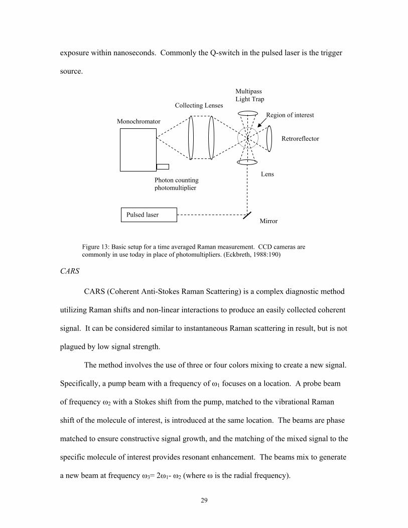
exposure within nanoseconds. Commonly the Q-switch in the pulsed laser is the trigger

source.

Pulsed laser Mirror

Multipass Light Trap

Lens

Retroreflector

Collecting Lenses

Monochromator

Photon counting photomultiplier

Region of interest

Figure 13: Basic setup for a time averaged Raman measurement. CCD cameras are commonly in use today in place of photomultipliers. (Eckbreth, 1988:190)

CARS

CARS (Coherent Anti-Stokes Raman Scattering) is a complex diagnostic method

utilizing Raman shifts and non-linear interactions to produce an easily collected coherent

signal. It can be considered similar to instantaneous Raman scattering in result, but is not

plagued by low signal strength.

The method involves the use of three or four colors mixing to create a new signal.

Specifically, a pump beam with a frequency of ω1 focuses on a location. A probe beam

of frequency ω2 with a Stokes shift from the pump, matched to the vibrational Raman

shift of the molecule of interest, is introduced at the same location. The beams are phase

matched to ensure constructive signal growth, and the matching of the mixed signal to the

specific molecule of interest provides resonant enhancement. The beams mix to generate

a new beam at frequency ω3= 2ω1- ω2 (where ω is the radial frequency).

29

The beam mixing occurs through the third order nonlinearity of the electric

susceptibility. Susceptibility is the ease of a material’s polarization in response to an

bility

e

ulting

ies

tage of

f magnitude greater than Raman scattering at

tmosp

hus

ds

usly. It works well with non-reacting

flows i ic

electric field, such as that created by the propagation of light photons. This suscepti

is dependent on density and temperature of the medium. The nonlinear response of th

matter incident to the incoming beams generates an oscillating polarization at the

frequency ω3. The mixing is termed third order because the oscillating polarization is

generated in the third order non-linear term of the susceptibility equation. The res

signal is a coherent radiation containing information useful to the measurement of spec

concentration (due to the Raman shift), temperature and density with good signal

strength. (Eckbreth, 1988:23, 226)

This improvement on signal strength in a coherent form is the major advan

CARS. The signal is many orders o

a heric pressure is. The coherence of the resulting radiation also improves the

signal to interference ratio as the complete signal can be captured in a small angle,

therefore limiting the amount of interference. The signal is anti-Stokes shifted, and t

also free from many fluorescent interferences (see Figure 12). Its ease of use excee

other coherent Raman techniques, and it is the diagnostic of choice for most harsh,

practical and dirty combustion environments.

The process is best suited for measurements of major species and thermometry

(Eckbreth, 1988:223), and does both simultaneo

n temperatures from below ambient to 3000K and pressures from sub-atmospher

to 100 bars. The reported accuracy is often within 2%, and it is successful for both

turbulent, time varying applications and steady phenomena (AIAA Reference Sheet).

30

The universality of the vibrational modes responding to the Raman Effect means the

technique is applicable to any molecule requiring obtainable light frequencies. The mo

common molecule probed is N

st

,

ty: First, the probe beam is specific to only one species, therefore another

probe b l

data.

aman.

2, but other typical species for combustion include H2O

CO, CO2, C2H2 and CH4. As with Raman, CARS temperature is determined from the

shape of the spectral distribution, and concentration of species is dependent on signal

strength. However, uniquely to CARS, the spectral distribution is often concentration

sensitive.

There are many disadvantages to this process as well, most of them arising from

its complexi

eam must be introduced to obtain good multiple-species data. The coherent signa

is directed away from the incident beams, therefore through optical access is necessary.

Phase matching is necessary in any three or more color technique, and adds to the

technique’s complexity. Also, the resulting spectra are very complex relative to

instantaneous Raman and sophisticated programs must be employed to analyze the

Finally, CARS species concentration sensitivity is on the order of instantaneous R

This means it is relatively insensitive compared to other techniques. Thus, it is only

useful for major species exceeding 0.1% concentration in the probed volume.

31

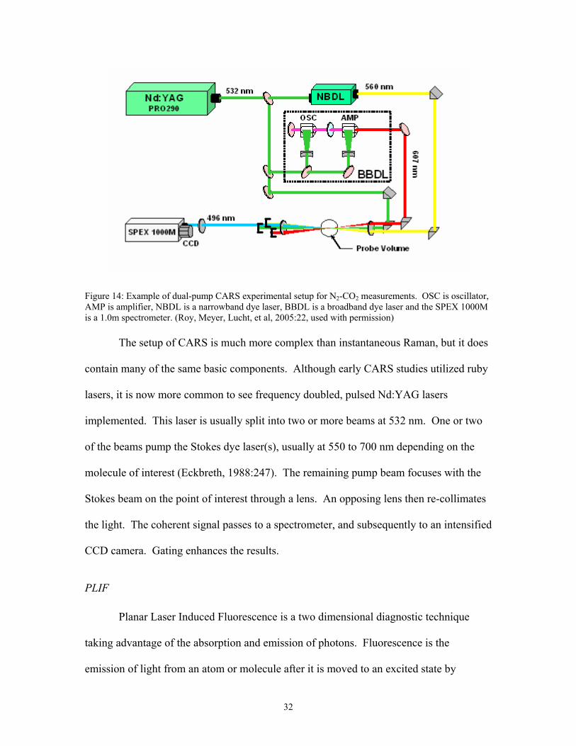
Figure 14: Example of dual-pump CARS experimental setup for N2-CO2 measurements. OSC is oscillator, AMP is amplifier, NBDL is a narrowband dye laser, BBDL is a broadband dye laser and the SPEX 1000M is a 1.0m spectrometer. (Roy, Meyer, Lucht, et al, 2005:22, used with permission)

The setup of CARS is much more complex than instantaneous Raman, but it does

contain many of the same basic components. Although early CARS studies utilized ruby

lasers, it is now more common to see frequency doubled, pulsed Nd:YAG lasers

implemented. This laser is usually split into two or more beams at 532 nm. One or two

of the beams pump the Stokes dye laser(s), usually at 550 to 700 nm depending on the

molecule of interest (Eckbreth, 1988:247). The remaining pump beam focuses with the

Stokes beam on the point of interest through a lens. An opposing lens then re-collimates

the light. The coherent signal passes to a spectrometer, and subsequently to an intensified

CCD camera. Gating enhances the results.

PLIF

Planar Laser Induced Fluorescence is a two dimensional diagnostic technique

taking advantage of the absorption and emission of photons. Fluorescence is the

emission of light from an atom or molecule after it is moved to an excited state by

32

various means. In the case of laser diagnostics, photon absorption is the preferred means

of excitation. Simply put, in fluorescence the atom or molecule absorbs an incident

photon, this in turn forces the electrons in upper levels to higher energy states, as shown

in Figure 12. In an effort to return to an equilibrium electron configuration, the atom or

molecule releases another photon at a different wavelength. Fluorescence is the term for

the specific case where emission occurs between electronic energy states of the same

multiplicity, or spin. This is opposed to phosphorescence, where emission occurs

between states of opposite spin. Fluorescent lifetimes are several orders of magnitude

longer than Raman scattering, varying between 10-10 and 10-5 seconds (Eckbreth,

1988:14). As shown in Figure 15 emitted light may be at a Stokes shifted frequency or it

may be at a resonant fluorescent frequency matching the incident beam. Usually, the

shifted frequency is utilized for measurements, as it reduces interferences with particle

scattering.

33

Fluorescence

Laser λ

Figure 15: Fluorescent absorption, emission and resulting spectra. The upper diagram indicates two electronic energy states with vibrational energy levels. Upward arrows indicate increasing energy. The symbol λ indicates signal wavelength. (Eckbreth, 1988:11)

As with Raman scattering, the resultant signal occurs in all directions and is

incoherent. Also as with Raman, the quantization of molecular and atomic energy states

results in discrete regions of spectral absorption. This means fluorescence is species

specific. The intensity of the signal is a generally linear function of number density of a

given species and is a function of temperature and pressure.

Unlike Raman scattering, the use of fluorescent techniques requires consideration

of quenching. Quenching has a large affect on the strength of the signal emitted, and its

variability can make data very uncertain. If detailed quenching data and the

concentration of quenching species is known, then analytical models can be used to

adjust for quenching affects. However, this is rarely the case. Thus, fluorescent

34

techniques often involve partial or complete saturation of the medium under study. This

eliminates quenching issues by permitting corrections to be determined in-situ.

PLIF takes advantage of fluorescence in a particularly useful way. Using

cylindrical optics the laser source is projected as a sheet into the region of interest. The

beam is usually pulsed and tunable to a wavelength resonant with the optical transition of

the species of interest. Because of this resonance, a fraction of the light will be absorbed

at each point the species resides within the laser sheet, another fraction of these photons

emit in fluorescence at the shifted wavelengths. A solid-state array camera collects the

light. The intensity of the fluorescence in the volume relates to the amount of light

captured by the camera at a corresponding location. Thus, the concentration of a

particular species, temperature, and pressure is measured. Utilizing the Doppler shift of

the signal, velocity measurements can be taken.

Flow fields are often measured using PLIF by seeding with an appropriate

substance that will fluoresce. In the case of combustion diagnostics, this is usually

unnecessary as concentrations of good fluorescing compounds such as Na, OH, NO, O2,

CH, CO and acetone are already present. OH is an important and plentiful radical in

combustion sequences, and is therefore often used as a flame locator. NO is often

imaged to determine locations of NOX production.

35

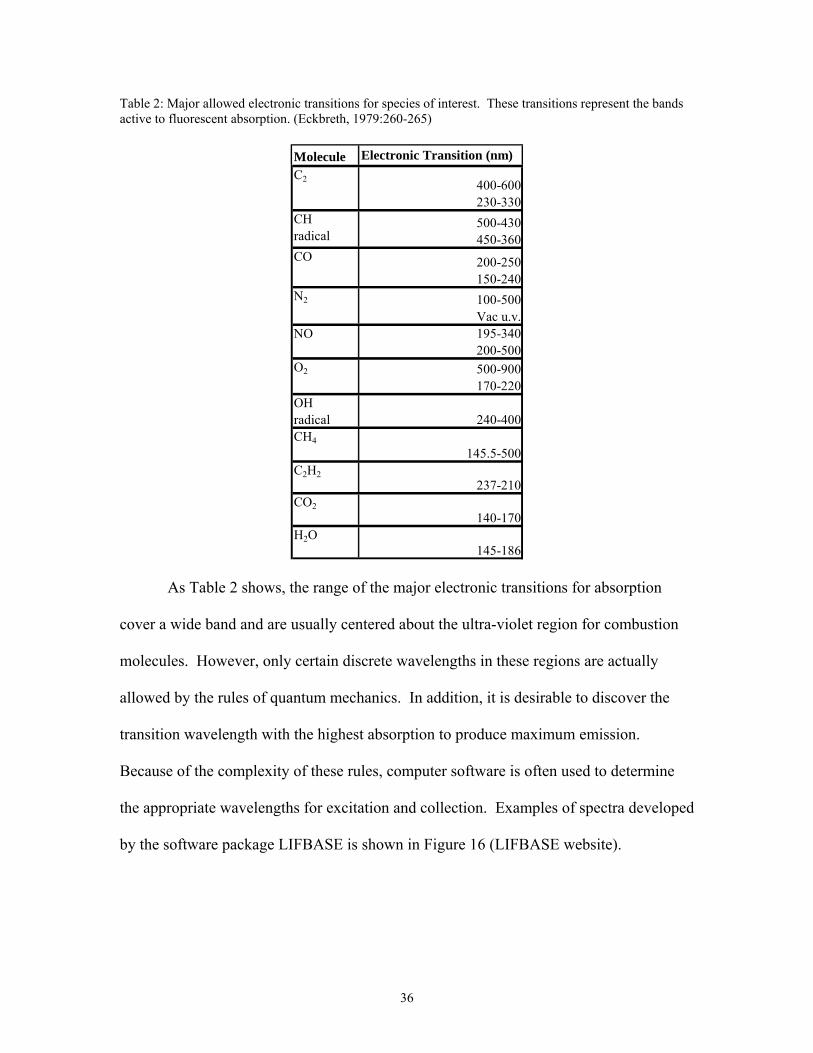
Table 2: Major allowed electronic transitions for species of interest. These transitions represent the bands active to fluorescent absorption. (Eckbreth, 1979:260-265)

Molecule Electronic Transition (nm)

400-600 230-330

CH radical

500-430 450-360

CO 200-250 150-240

C2

100-500 Vac u.v.

NO 195-340 200-500

O2 500-900 170-220

N2

OH radical 240-400CH4

145.5-500

H2O145-186

C2H2237-210

CO2140-170

As Table 2 shows, the range of the major electronic transitions for absorption

cover a wide band and are usually centered about the ultra-violet region for combustion

molecules. However, only certain discrete wavelengths in these regions are actually

allowed by the rules of quantum mechanics. In addition, it is desirable to discover the

transition wavelength with the highest absorption to produce maximum emission.

Because of the complexity of these rules, computer software is often used to determine

the appropriate wavelengths for excitation and collection. Examples of spectra developed

by the software package LIFBASE is shown in Figure 16 (LIFBASE website).

36

285 nm 280 nm 290 nm

OH Absorption Spectra OH Emission Spectra

310 nm 305 nm 315 nm

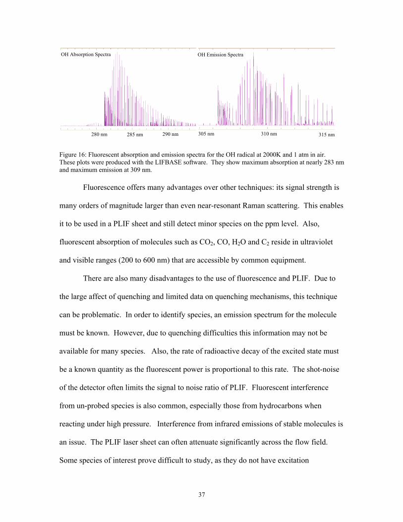
Figure 16: Fluorescent absorption and emission spectra for the OH radical at 2000K and 1 atm in air. These plots were produced with the LIFBASE software. They show maximum absorption at nearly 283 nm and maximum emission at 309 nm. Fluorescence offers many advantages over other techniques: its signal strength is

many orders of magnitude larger than even near-resonant Raman scattering. This enables

it to be used in a PLIF sheet and still detect minor species on the ppm level. Also,

fluorescent absorption of molecules such as CO2, CO, H2O and C2 reside in ultraviolet

and visible ranges (200 to 600 nm) that are accessible by common equipment.

There are also many disadvantages to the use of fluorescence and PLIF. Due to

the large affect of quenching and limited data on quenching mechanisms, this technique

can be problematic. In order to identify species, an emission spectrum for the molecule

must be known. However, due to quenching difficulties this information may not be

available for many species. Also, the rate of radioactive decay of the excited state must

be a known quantity as the fluorescent power is proportional to this rate. The shot-noise

of the detector often limits the signal to noise ratio of PLIF. Fluorescent interference

from un-probed species is also common, especially those from hydrocarbons when

reacting under high pressure. Interference from infrared emissions of stable molecules is

an issue. The PLIF laser sheet can often attenuate significantly across the flow field.

Some species of interest prove difficult to study, as they do not have excitation

37

frequencies commonly available from a single source. In fact, temperature measurements

usually require two laser sources and homonuclear radicals such as C2 cannot be detected

(AIAA Reference sheet). Research has shown that velocity measurements are usually

only practical for high Mach number flows. Fluorescence runs a higher risk of laser-

induced chemistry, although this is normally avoided with the use of faster (nanosecond)

pulsed lasers (Eckbreth, 1988:305). Finally, the use of laser sheets usually requires

optical access at perpendicular orientations to capture results.

The general setup of PLIF is similar to the other laser techniques. Again a pulsed,

frequency doubled Nd:YAG laser is commonly used to pump a dye laser. The resultant

beam usually passes through a frequency conversion assembly in order to produce the

required frequency for fluorescence of the molecule of interest. In PLIF a cylindrical

lens then creates a laser sheet photographed by a high resolution or intensified CCD

camera in a position approximately perpendicular to the sheet. The camera is gated and

timed, usually off the Q-switch of the source laser.

Figure 17: Schematic of experimental setup for conducting simultaneous LII and OH PLIF measurements. The OH PLIF is provided by the pumped dye laser at 284 nm. (Meyer and Roy, 26:2003, used with permission)

38

LII

Laser Induced-Incandescence (LII) uses the release of blackbody radiation to

track particulates in a flow field. Incandescence is the release of electromagnetic

radiation from a hot body at a high temperature, such as a filament in a light bulb.

Photons emit when electrons jump to higher states due to the energy absorbed by the

heating process. This phenomena occurs for all matter, but is usually in the infrared

spectrum, and thus invisible to the naked eye below 900K. The intensity of emission

increases with temperature, with the peak signal wavelength shifting towards smaller

wavelengths (blue) according to the Planck radiation law.

For combustion diagnostics, this technique is of use for determining the volume

fraction of soot in the flow. If a laser of sufficient energy is used, the pulsed light can

heat soot particles of typical size (20 to 50 nm) so they incandesce in a blue shifted

frequency, even inside the flame. This blue light is detected easily when captured before

cooling occurs within nanoseconds of the laser pulse (Vander Wal, 1997:1). Theory

predicts the intensity of this incandescence correlates to soot volume fraction. This is

because the soot particles are much smaller than the laser excitation wavelength, and thus

can be considered volume absorbers. However, in reality the soot is not a perfect volume

absorber. Thus, calibration is used to determine the exact volume fraction (Wainner,

1997:2), with uncertainties of the order of 10% (AIAA Reference Sheet). This process

has also been used in a limited manner to determine the size of soot agglomerates.

LII has multiple advantages. It is well suited for both steady and rapidly changing

phenomena as observations can be made from a single laser pulse. This is usually every

10 ns (Vander Wal, 1997:1). Spatial resolution is also good. The process is nearly

39

independent of scattering by aggregates and absorption of polycyclic aromatic

hydrocarbons (PAH’s), molecular fluorescence or flame luminance. The technique

requires no through optical access. Planar measurements are possible and commonly

used with the creation of a laser sheet.

The major disadvantages include the requirement of calibration. Measurement

uncertainty increases with deviation of actual conditions from temperature and soot

agglomerate size used in calibration. Although most fluorescence is not an issue, some

types can interfere with the LII signal. Also, inconsistent particle heating can be

problematic. Like PLIF, high particulate concentrations and long beam path lengths can

cause attenuation of incident beam or LII signal across the measurement volume. This

introduces errors to the readings. The process also requires use of a higher intensity

laser, at least 50 to 100MW/cm2. Fast gating detectors are also necessary (less than 50 ns

for lasers with 5-10 ns pulse durations).

LII setup uses similar equipment to the other techniques discussed. In this case it

is not uncommon to use a pulsed Nd:YAG laser at its normal frequency of 1064 nm

(infrared) although other sources are also used at 532 nm. The most important aspect is

the beam must have sufficient power to heat the soot particles quickly. From this beam a

laser sheet, as seen in Figure 17 or small investigation volume is made using an

appropriate lens. Bandpass filters block light outside of the blue wavelengths of interest

for collection. A CCD camera or monochromator with photomultiplier tube capture the

LII signal. Like all other techniques, gating improves the signal reading.

40

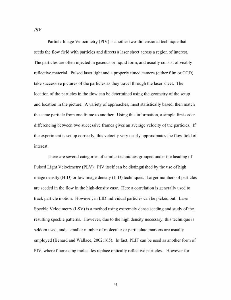
PIV

Particle Image Velocimetry (PIV) is another two-dimensional technique that

seeds the flow field with particles and directs a laser sheet across a region of interest.

The particles are often injected in gaseous or liquid form, and usually consist of visibly

reflective material. Pulsed laser light and a properly timed camera (either film or CCD)

take successive pictures of the particles as they travel through the laser sheet. The

location of the particles in the flow can be determined using the geometry of the setup

and location in the picture. A variety of approaches, most statistically based, then match

the same particle from one frame to another. Using this information, a simple first-order

differencing between two successive frames gives an average velocity of the particles. If

the experiment is set up correctly, this velocity very nearly approximates the flow field of

interest.

There are several categories of similar techniques grouped under the heading of

Pulsed Light Velocimetry (PLV). PIV itself can be distinguished by the use of high

image density (HID) or low image density (LID) techniques. Larger numbers of particles

are seeded in the flow in the high-density case. Here a correlation is generally used to

track particle motion. However, in LID individual particles can be picked out. Laser

Speckle Velocimetry (LSV) is a method using extremely dense seeding and study of the

resulting speckle patterns. However, due to the high density necessary, this technique is

seldom used, and a smaller number of molecular or particulate markers are usually

employed (Benard and Wallace, 2002:165). In fact, PLIF can be used as another form of

PIV, where fluorescing molecules replace optically reflective particles. However for

41

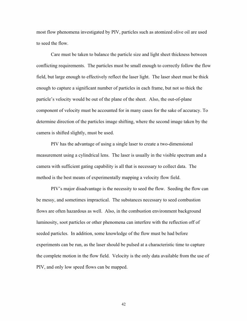
most flow phenomena investigated by PIV, particles such as atomized olive oil are used

to seed the flow.

Care must be taken to balance the particle size and light sheet thickness between

conflicting requirements. The particles must be small enough to correctly follow the flow

field, but large enough to effectively reflect the laser light. The laser sheet must be thick

enough to capture a significant number of particles in each frame, but not so thick the

particle’s velocity would be out of the plane of the sheet. Also, the out-of-plane

component of velocity must be accounted for in many cases for the sake of accuracy. To

determine direction of the particles image shifting, where the second image taken by the

camera is shifted slightly, must be used.

PIV has the advantage of using a single laser to create a two-dimensional

measurement using a cylindrical lens. The laser is usually in the visible spectrum and a

camera with sufficient gating capability is all that is necessary to collect data. The

method is the best means of experimentally mapping a velocity flow field.

PIV’s major disadvantage is the necessity to seed the flow. Seeding the flow can

be messy, and sometimes impractical. The substances necessary to seed combustion

flows are often hazardous as well. Also, in the combustion environment background

luminosity, soot particles or other phenomena can interfere with the reflection off of

seeded particles. In addition, some knowledge of the flow must be had before

experiments can be run, as the laser should be pulsed at a characteristic time to capture

the complete motion in the flow field. Velocity is the only data available from the use of

PIV, and only low speed flows can be mapped.

42

PIV setup requires some differing equipment than other combustion techniques.

The diagnostic uses light at visible wavelengths such as 532 nm or 355nm. These may be

created by a Nd:YAG signal that is mixed using harmonic crystals. If the beam is not

pulsed, a shutter mechanism may be used. Also, the laser beam is often passed onto a

mechanical device to provide image shifting by timed rotation of mirrors so velocity

direction can be assessed. From here, a lens creates a laser sheet across the flow of

interest and a film or CCD camera is used to take pictures of the flow in rapid succession.

Timing is important in PIV as well, but more so for temporal resolution of the photos to

determine the flow field than improving signal collection. An appropriately designed

flow seeder is also necessary in PIV.

43

III. Methodology

3.1 System Design and Operation

The laboratory is located in room 258 of building 640 at the Air Force Institute of

Technology. It is designed to facilitate small-scale combustion experimentation at

atmospheric pressure. The facility features five central elements: First, a computer

control station provides remote operation and data collection for experiments (seen in

Figure 18). Secondly, a laser diagnostic system enables advanced data collection such as

PIV and PLIF. Third, various operation and measurement systems throughout the room

give basic functionality to the lab. Fourth, a combustor stand gives a place to physically

mount the combustor, and support equipment. Finally, a Unistrut cage, 20 feet by 10

feet, encloses the experimental area, and provides support for wires, tubes and cables.

This clears the floor of clutter and enables the easy location of the laser diagnostic

system.

Figure 18: California Analytical Instruments raw exhaust analyzer test bench (l) and laboratory computer control station (r).

44

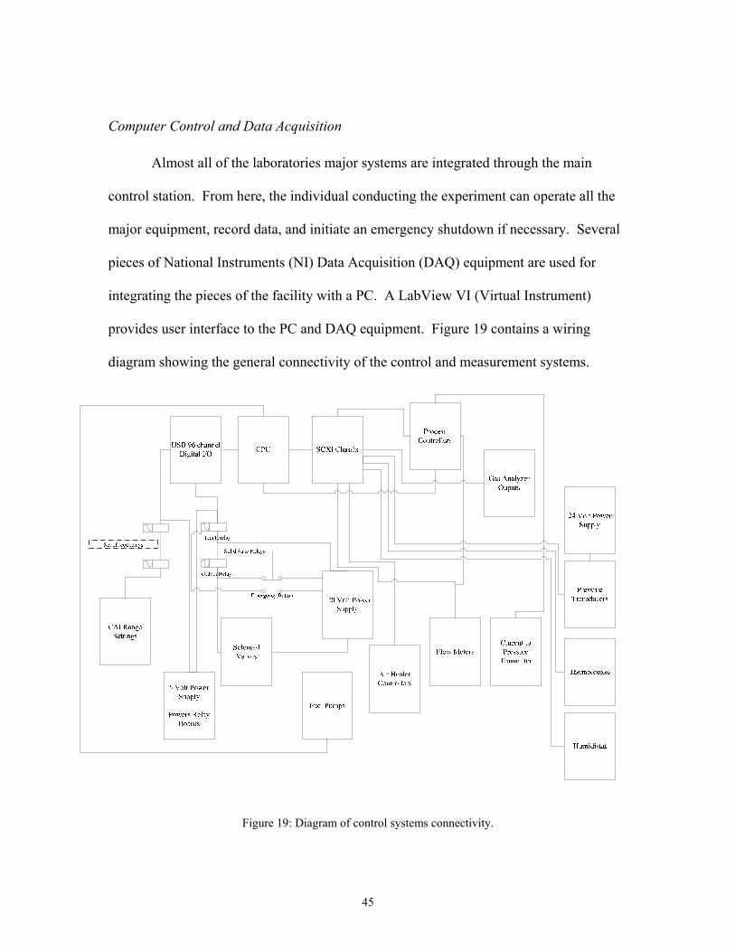
Computer Control and Data Acquisition

Almost all of the laboratories major systems are integrated through the main

control station. From here, the individual conducting the experiment can operate all the

major equipment, record data, and initiate an emergency shutdown if necessary. Several

pieces of National Instruments (NI) Data Acquisition (DAQ) equipment are used for

integrating the pieces of the facility with a PC. A LabView VI (Virtual Instrument)

provides user interface to the PC and DAQ equipment. Figure 19 contains a wiring

diagram showing the general connectivity of the control and measurement systems.

Figure 19: Diagram of control systems connectivity.

45

An HP dx5150 MT PC operating with Windows XP and installed with LabView

8.2 is the brain of the laboratory. It is located in an electrical enclosure containing most

of the electronics hardware. Two devices connect the PC to the laboratory through USB.

The first is a National Instruments (NI) SCXI-1600 USB 16-Bit digitizer module. This

unit mounts in and provides control of the NI SCXI 1100 Data Acquisition (DAQ)

chassis. The chassis acts as an interface with many interchangeable hardware modules.

The modules in turn are interchangeable with a limited number of terminal blocks. These

terminal blocks connect directly to the equipment throughout the laboratory through

signal or thermocouple lines. Most of the information sent by the laboratories

measurement equipment are received by the terminal blocks with 4-20mA signals.

Control of rig air heaters and the flow control loop is acomplished via 0-5 VDC output

signals. Figure 20 shows a detail of the chassis setup. Appendix A details all of the

nearly 100 electronic signal connections in the laboratory running through the SCXI 1100

chassis. For ease of installation and modification, spring release wire connecting

terminal blocks mounted in the enclosure provide a break in each signal line between the

NI terminal blocks and laboratory equipment.

The second device connecting the PC to the laboratory is a NI DAQPad 6508.

This device provides digital I/O capability controling two Opto 22 Solid State Relay

(SSR) boards. A diagram of the connection of this hardware is shown in Figure 20.

These boards act as computer controlled on-off switches for equipment throughout the

lab. The first of these boards, the PB24, controls all solenoid valves and the ignition

transformer. It also reads inputs from a pressure switch in the exhaust ducts (to ensure

the exhaust is operating) and the emergency-shutdown switch (to inform the computer

46

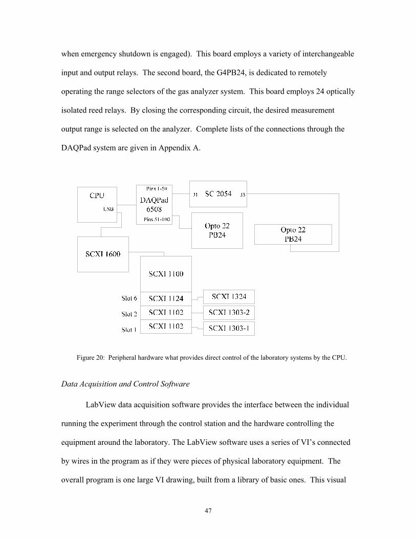
when emergency shutdown is engaged). This board employs a variety of interchangeable

input and output relays. The second board, the G4PB24, is dedicated to remotely

operating the range selectors of the gas analyzer system. This board employs 24 optically

isolated reed relays. By closing the corresponding circuit, the desired measurement

output range is selected on the analyzer. Complete lists of the connections through the

DAQPad system are given in Appendix A.

Figure 20: Peripheral hardware what provides direct control of the laboratory systems by the CPU.

Data Acquisition and Control Software

LabView data acquisition software provides the interface between the individual

running the experiment through the control station and the hardware controlling the

equipment around the laboratory. The LabView software uses a series of VI’s connected

by wires in the program as if they were pieces of physical laboratory equipment. The

overall program is one large VI drawing, built from a library of basic ones. This visual

47

programming allows the code to be quickly understood by a new user who may want to

modify the program. When the main LabView VI is running, a front panel is displayed

on the computer’s screen. Much like a real instrument, the VI’s front panel consists of

buttons, switches and displays the user can interact with while the program is operating.

Dittman developed the code’s organizing structure and most of the programming.

However, much troubleshooting, adaptation to systems, connectivity, and modification

for usability was completed in the author’s work.

Through use of this software, the user can control all systems connected to the

computer and automatically record pressure, temperature and emissions data for later

analysis. Thus, the LabView VI makes the laboratory easily manageable. A flow chart

demonstrating the operation of the software is shown in Figure 21.

48

Figure 21: Combustion facility control software flow of operation. (Dittman, 2006:32)

49

Power supply systems

Power for most laboratory equipment is routed through the control station. Most

devices operate on a standard 120VAC/60Hz supply. However, both 5 and 24VDC are

provided from the enclosure for varied equipment. The distribution of this power is

provided by several terminal blocks, mounted in the electrical enclosure. Figure 22

shows the wiring of both AC power, Figure 23 shows DC. A complex series of signal

connections also provides power for the various pressure transducers located in two

boxes in the lab, this can be seen in Figure 24.

All AC power used to control valves supplying the combustor system is wired

directly through an emergency shutoff button. This is located on the enclosure at the

operator’s station. The direct connection ensures no hang-ups in the event of an

emergency. All systems have been designed for a flameout emergency shutdown. The

switch is also wired through the 24 VDC power supply and one of the input relays on the

PB24 so the computer can sense an emergency shutdown.

50

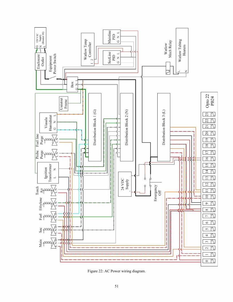
Figure 22: AC Power wiring diagram.

51

5 V Power Distribution5 VDC Supply

Pressure Transducer

Box 1

Pressure Transducer

Box 2

1 2 3 4 16 175 109876 1211 13 14 15 18 19 20 21 22 230 Opto 22 PB24

24 V Power Distribution24 VDC Supply

Opto 22G4PB24

MainHeater Control

UT420 1821

SecondaryHeater Control

UT420 1821

Emergency Off

Figure 23: DC power wiring diagram.

52

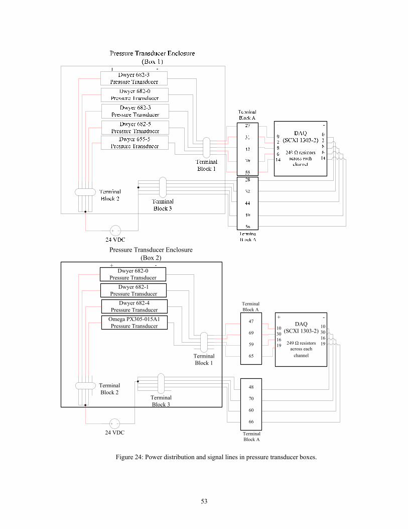
Dwyer 682-0Pressure Transducer

TerminalBlock 1

DAQ(SCXI 1303-2)

249 Ω resistors across each

channel

TerminalBlock 3

TerminalBlock 2

24 VDC

+

Dwyer 682-1Pressure Transducer

Omega PX305-015A1Pressure Transducer

Dwyer 682-4Pressure Transducer

+ -

-

Pressure Transducer Enclosure (Box 2)

47

69

59

65

TerminalBlock A

1030 1619

1030 1619

48

70

60

66

TerminalBlock A

Figure 24: Power distribution and signal lines in pressure transducer boxes.

53

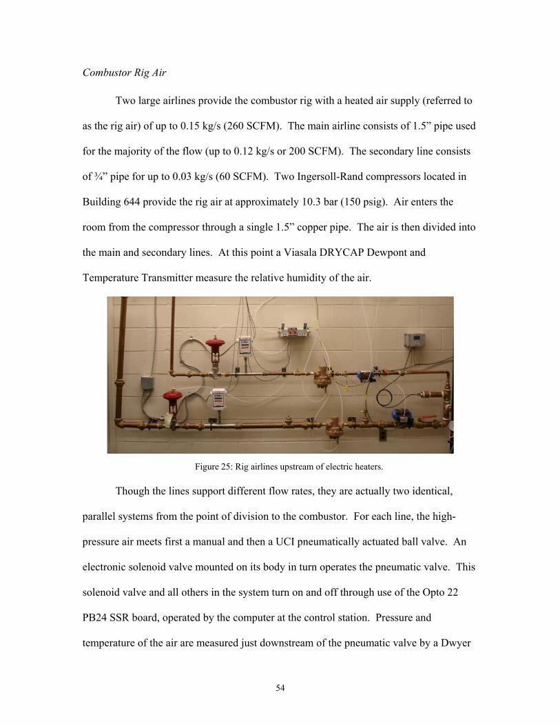
Combustor Rig Air

Two large airlines provide the combustor rig with a heated air supply (referred to

as the rig air) of up to 0.15 kg/s (260 SCFM). The main airline consists of 1.5” pipe used

for the majority of the flow (up to 0.12 kg/s or 200 SCFM). The secondary line consists

of ¾” pipe for up to 0.03 kg/s (60 SCFM). Two Ingersoll-Rand compressors located in

Building 644 provide the rig air at approximately 10.3 bar (150 psig). Air enters the

room from the compressor through a single 1.5” copper pipe. The air is then divided into

the main and secondary lines. At this point a Viasala DRYCAP Dewpont and

Temperature Transmitter measure the relative humidity of the air.

Figure 25: Rig airlines upstream of electric heaters.

Though the lines support different flow rates, they are actually two identical,

parallel systems from the point of division to the combustor. For each line, the high-

pressure air meets first a manual and then a UCI pneumatically actuated ball valve. An

electronic solenoid valve mounted on its body in turn operates the pneumatic valve. This

solenoid valve and all others in the system turn on and off through use of the Opto 22

PB24 SSR board, operated by the computer at the control station. Pressure and

temperature of the air are measured just downstream of the pneumatic valve by a Dwyer

54

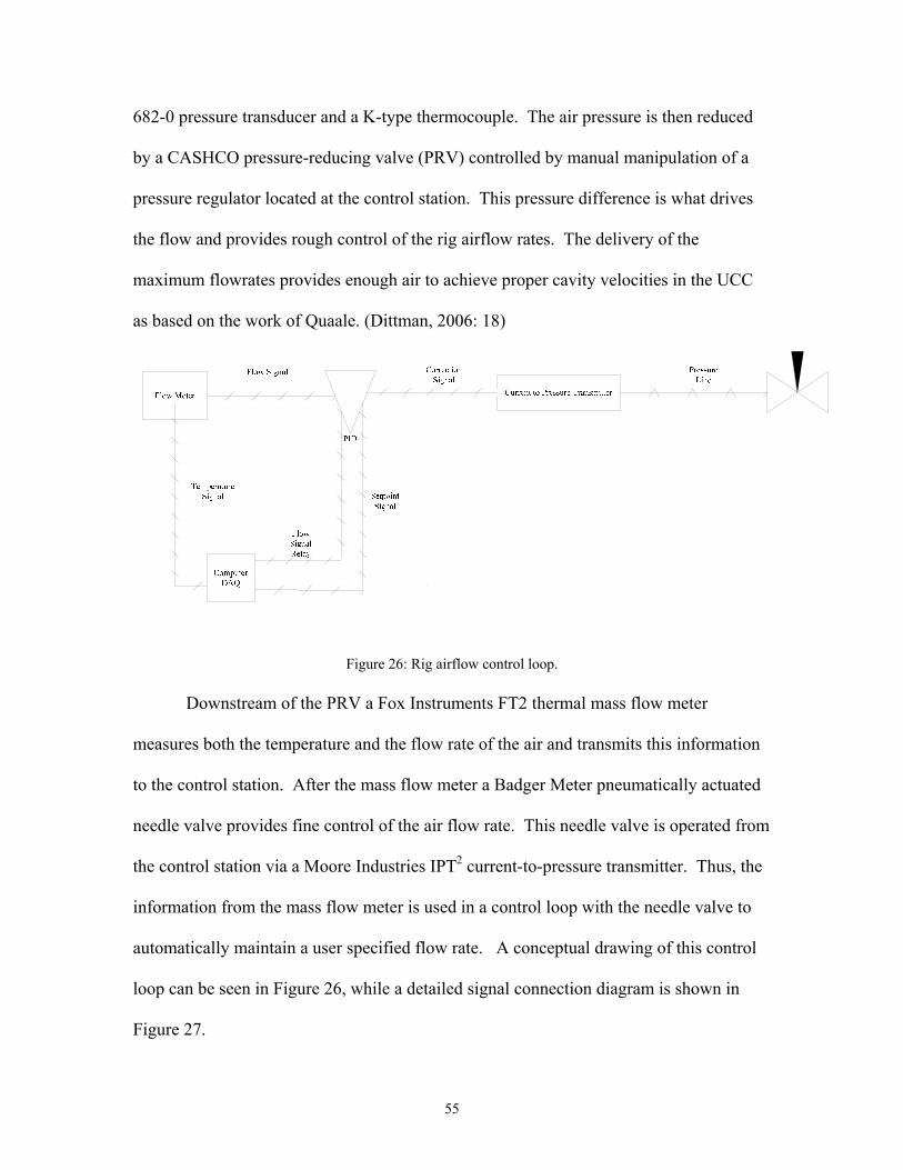
682-0 pressure transducer and a K-type thermocouple. The air pressure is then reduced

by a CASHCO pressure-reducing valve (PRV) controlled by manual manipulation of a

pressure regulator located at the control station. This pressure difference is what drives

the flow and provides rough control of the rig airflow rates. The delivery of the

maximum flowrates provides enough air to achieve proper cavity velocities in the UCC

as based on the work of Quaale. (Dittman, 2006: 18)

Figure 26: Rig airflow control loop.

Downstream of the PRV a Fox Instruments FT2 thermal mass flow meter

measures both the temperature and the flow rate of the air and transmits this information

to the control station. After the mass flow meter a Badger Meter pneumatically actuated

needle valve provides fine control of the air flow rate. This needle valve is operated from

the control station via a Moore Industries IPT2 current-to-pressure transmitter. Thus, the

information from the mass flow meter is used in a control loop with the needle valve to

automatically maintain a user specified flow rate. A conceptual drawing of this control

loop can be seen in Figure 26, while a detailed signal connection diagram is shown in

Figure 27.

55

-+

TS1

TS21 +2 -3 +4 -5 +6 -

33 (49)

34 (50)

35 (51)

36 (52)

79 (81)

80 (82)

Terminal Block A

DAQ(SCXI 1303-2)

Temp3 (11) +

3 (11) -Flow

4 (12) +

4 (12) -

DAQ(SCXI 1325)

Setpoint Out0 (1) Supply

0 (1) I Sink

IPT2

Current to Pressure Transmitter

GC Controls2404 PID Controller

LNG

Flow Rate V+V-

Control Out to IPT1A + 1B -

Flow Rate Retransmit2A +2B -

0-5VDC Setpoint3A +

3D -

Main flow connection # (Secondary flow connection #)

Temperature

Flow Rate

2.49

Fox Box Flow Meter

+ IN

- IN

Needle Valve

Instrument Air System

Meter Entrance

Meter Exit

Airline to Combustor

Airline fromInlet

249

249

249

Figure 27: Signal line connection schematic of rig air control loop and data transmission.

In this control loop, the mass flow rate is transmitted to a GC Controls 2404 PID

controller mounted at the control station. The PID in turn retransmits this information to

the computer for use in data recording and easy user monitoring. After closing in on the

desired flow rate with adjustment of the PRV regulator the user can specify the desired

flow rate exactly in the LabView VI. This set point information is transmitted to the PID

through the NI SCXI 1325 Low Voltage terminal block. The PID then uses proportional-

integral-derivative logic to achieve the set point by sending a correction signal to the

56

current-to-pressure transmitter. This in turn controls the needle valve. By constantly

updating this process, the flow rate of each rig airline is maintained.

At this point, the air is nearly atmospheric in pressure and is traveling at the

desired mass flow rate. It then enters a Gaumer electric air heater. This device can raise

the air temperature up to 810K (1000 °F). However, the flexible tubing connection to

the combustor can only tolerate 530K (500°F) and the Teflon pipe dope used to seal the

airlines can only withstand 670K (750°F). This heating simulates air exiting a

compressor. The heater receives a temperature set point from the control station through

the NI SCXI 1325 module and contains its own PID, internally adjusting the heater

temperature. This temperature is retransmitted to the computer for data recording. As

seen in Figure 28, an emergency shutoff for the heaters is also operated at the control

station through the PB24 SSR board. Once the rig air passes through the heaters it feeds

through insulated stainless steel lines directly to the combustor for use. At the end of

these lines, two high temperature hoses provide flexibility for connection.

57

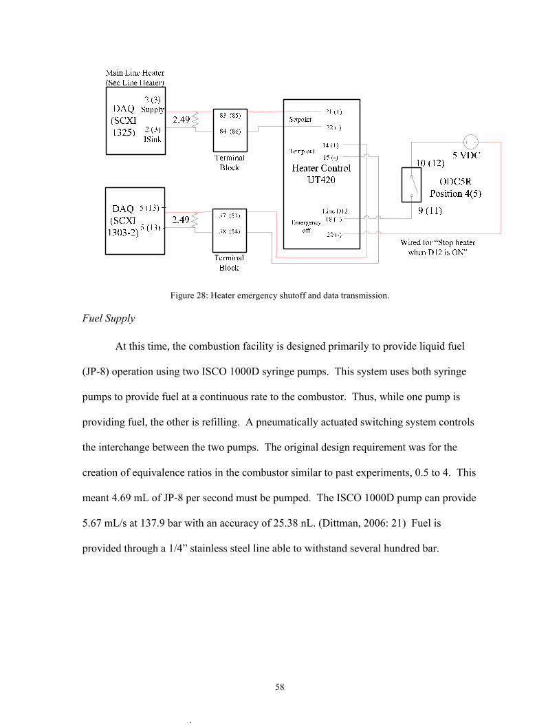
Figure 28: Heater emergency shutoff and data transmission.

Fuel Supply

At this time, the combustion facility is designed primarily to provide liquid fuel

(JP-8) operation using two ISCO 1000D syringe pumps. This system uses both syringe

pumps to provide fuel at a continuous rate to the combustor. Thus, while one pump is

providing fuel, the other is refilling. A pneumatically actuated switching system controls

the interchange between the two pumps. The original design requirement was for the

creation of equivalence ratios in the combustor similar to past experiments, 0.5 to 4. This

meant 4.69 mL of JP-8 per second must be pumped. The ISCO 1000D pump can provide

5.67 mL/s at 137.9 bar with an accuracy of 25.38 nL. (Dittman, 2006: 21) Fuel is

provided through a 1/4” stainless steel line able to withstand several hundred bar.

58

.

Figure 29: Liquid fuel pump and control system

As shown in Figure 29, the pumps are controlled through a serial connection

directly to the PC and the LabView software interface. This LabView pump control

program was provided by ISCO and integrated into the laboratory control VI. In

addition, another UCI pneumatic valve controlled by an offset Hoerbiger solenoid valve

is connected downstream of the fuel pump. The SSR PB24 board operates this too. This

UCI valve acts as the emergency shutoff valve for the fuel system. Manual valves

located just upstream of the fuel pump, downstream of the pneumatic ball valve and near

the combustor stand provide control for fuel line disconnect, purging and emergency

shut-off. A pressure tap runs to a Dwyer 682-4 pressure transmitter, and another K-type

thermocouple measures the temperature of the fuel line. Thus, the state of the fuel at

combustor entry is known.

59

Figure 30: ISCO fuel pump system.

Remote Ignition

For remote ignition of the combustor, an ethylene/air torch was built to attach to

one of the combustor sidewalls. Fuel is deposited in this region, and experience with

similar laboratory environments suggests this is the ideal location for ignition. Air and

ethylene gas are stored in bottles in the bottle farm outside the building and piped in at

30-40 psig. To simplify system operation and reduce control problems from loss of

instrument air, bottled cylinder zero air is used as the oxidizer.

Both zero air and ethylene fuel are turned on and off by use of Parker solenoid

valves (again controlled by the SSR board). For safety, the ethylene solenoid valve is

explosion proof and placed above other nearby valves and electronics (ethylene is lighter

than air at room conditions). The equivalence ratio of the torch must by preset by two

60

metering valves located before the mixing point on the combustor stand. Check valves

prevent propagation of burning gases from the combustor into the supply lines. An AC

Delco R44LTSM automotive spark plug ignites the torch at the combustor. Electricity is

run through metallic, single conductor spark plug wire to provide remote ignition. A

Dongan A10-LA2 ignition transformer also wired through the SSR PB24 control board

provides sparking power. Grounding is provided through the combustor stand, and is

connected to the Unistrut laboratory frame. This in turn is earth grounded through the

electrical system. This grounding is common to the ignition transformer, as is necessary

for its proper operation.

Figure 31: Solenoid valves controlling ignition and purge systems and their connection to the combustor stand.

Nitrogen Purge

Bottled nitrogen is used to provide an inert purge of both the fuel line and the

emissions sample line. Purge of the fuel injector is critical to prevent coking or other

sources of flow degradation. Similarly, the emissions probe must be cleared to prevent

61

buildup that may block sampling. Nitrogen is provided to purge the fuel system by the

use of a four way union located on the combustor stand. One union connection provides

fuel from the pump through the 1/4” line. Two of the connections provide fuel to the

combustor through 1/8” stainless steel lines. The remaining connection provides the

nitrogen. Both the nitrogen and fuel lines have check valves preventing backflow of

nitrogen or fuel into the opposing systems.

The nitrogen supply is controlled by a normally-open Parker solenoid valve,

wired through the SSR control board. Thus, when the test is stopped by either

emergency, electrical outage or standard shutdown, power is cut from both the fuel line

emergency valve and the nitrogen control valve. This cuts fuel pressure on the fuel line

and engages the nitrogen line, purging the fuel injectors. Nitrogen is also supplied to the

fuel line near the fuel emergency shutoff valve to purge the majority of the fuel line

during maintenance.

The nitrogen supply is also connected to a UCI 3-way, pneumatically actuated

valve. Two of these valves run in series along the emissions line and are actuated by a

normally-open Parker solenoid valve, run through the SSR PB24 control board. Again,

when power is cut to the solenoid valve it in turn actuates both three way valves

pneumatically. This disconnects the emissions probe from the gas analyzer. Nitrogen

flows to the emissions probe and purges it, the rest of the emissions line is opened to the

atmosphere, through a filter, to allow for continued pumping by the gas analyzer system.

Figure 32 details the fluid systems running throughout the laboratory.

62

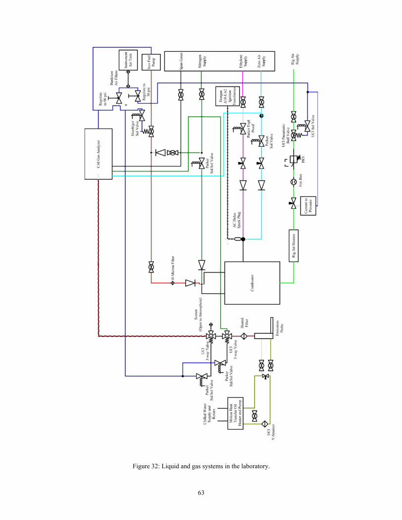
Figure 32: Liquid and gas systems in the laboratory.

63

Gas Analyzer

As discussed in previously, a California Analytical Instruments (CAI) Raw

Emissions Test Bench is used to analyze combustor emissions for products of interest.

These include total hydrocarbons (THC), nitrogen oxides (NOx), carbon dioxide (CO2),

carbon monoxide (CO), and oxygen (O2), and are measured by a Model 300 HFID, a

Model 400 HCLD, a Model 300 NDIR and a Model 300 paramagnetic oxygen detector

respectively. The theory behind the operation of these detectors is covered in chapter

two.

This emissions data must be taken reliably to produce useful results. The CAI gas

detectors making up the test bench fall within specifications for raw emissions

measurements as defined in SAE ARP 1256. (Dittman, 2006:23). The concentration of

these gases is of interest to the experiment, as they are used to determine the emissions

index, this in turn is used to determine the combustion efficiency.

The gas detectors require the use of calibration and span gases, purge air and

hydrogen-helium fuel for calibration and operation. With the exception of the purge air,

these substances are stored in compressed bottles outside of the laboratory building. The

pressure is regulated to the desired value at the bottle location, and then flows into the

laboratory through two bundles of seven 1/4” copper tubes. Purge air is provided through

the instrument air system. The mixture, required flow rates, delivery pressures and other

requirements for these gases are listed in Appendix A.

The CAI gas analyzer outputs the concentration of gases to digital displays

mounted on the front of its body. However, for data recording purposes and ease of

control this data is output by a 4-20mA signal to the DAQ and computer control system.

64

These signals are received by an NI 1303 Isothermal Terminal Block, and are displayed

and recorded to file with proper scaling via the LabView software. This software also

automatically controls the range setting of each detector. As seen in Table 3 the range

setting of each detector enables it to provide good resolution on the actual concentration

of the particular gas. Use of the G4PB24 solid-state relay board allows the computer to

control the range remotely.

Table 3: Ranges for gases analyzed by CAI test bench.

Gas Range Span1 0-5%2 0-10%3 0-25%1 0-2k ppm2 0-1%1 0-5%2 0-20%1 0-30 ppm2 0-100 ppm3 0-300 ppm4 0-1k ppm5 0-3k ppm1 0-10 ppm2 0-30 ppm3 0-100 ppm4 0-300 ppm5 0-1k ppm6 0-3k ppm7 0-10k ppm

Oxygen

CO

CO2

THC

NOX

Emissions Collection

The CAI gas analyzer receives the emissions from the combustor through the

emissions collection system. Exhaust exiting the combustor is collected using a stainless

steel exhaust probe. This probe (shown in Figure 33) has an approximately 1/8” diameter

opening to collect emissions. Because of the high temperature of the exhaust stream, the

65

probe is built with an enclosed heat exchanger that circulates heat transfer oil at

approximately 450K (350 °F) too cool the probe and maintain gas temperature.

Figure 33: Oil heated emissions probe and electrically heated line on test stand.

According to SAE ARP 1256, the emissions sample must be maintained at 433K

± 15K (320°F ± 27 °F). This is to keep any water in a completely gaseous state as it may

damage systems or skew data if it condenses in the sample line (SAE ARP 1256: Section

10.3). A Mokon H22103AJ Compact Heated Thermal Fluid System (shown in Figure

34) heats and circulates the oil at approximately 2.75 bar (40 psi). From the Mokon unit

3/8” stainless steel tubing provides oil supply and return lines. For proper operation of

the Mokon system, a laboratory wide chilled water system is connected to the unit. This

circulates a chilled water-glycol mixture at approximately 3.45 bar (50 psi) and 266K

(20°F).

66

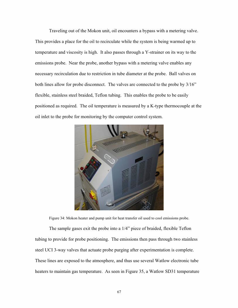
Traveling out of the Mokon unit, oil encounters a bypass with a metering valve.

This provides a place for the oil to recirculate while the system is being warmed up to

temperature and viscosity is high. It also passes through a Y-strainer on its way to the

emissions probe. Near the probe, another bypass with a metering valve enables any

necessary recirculation due to restriction in tube diameter at the probe. Ball valves on

both lines allow for probe disconnect. The valves are connected to the probe by 3/16”

flexible, stainless steel braided, Teflon tubing. This enables the probe to be easily

positioned as required. The oil temperature is measured by a K-type thermocouple at the

oil inlet to the probe for monitoring by the computer control system.

Figure 34: Mokon heater and pump unit for heat transfer oil used to cool emissions probe.

The sample gases exit the probe into a 1/4” piece of braided, flexible Teflon

tubing to provide for probe positioning. The emissions then pass through two stainless

steel UCI 3-way valves that actuate probe purging after experimentation is complete.

These lines are exposed to the atmosphere, and thus use several Watlow electronic tube

heaters to maintain gas temperature. As seen in Figure 35, a Watlow SD31 temperature

67

controller located at the computer station is used to maintain the tube heater’s

temperature. The control loop includes a solid-state relay and a K-type thermocouple.

Figure 35: Temperature control loop of exposed emissions line.

After the 3-way valves the gas enters a Unique Products International heated gas

filter and a 9 m (30 ft) heated line. The filter removes debris that may clog the transport

line or damage analyzer components. Two additional Watlow SD31 temperature

controllers also control the temperature of these systems. However, these are located in

the CAI gas analyzer test bench. Thermocouples have been pre-manufactured into both

items. The test bench also includes a pump that transports the gas from the probe to the

analyzer.

Instrument Air

A Kaeser compressor located in Building 644 provides instrument air at 6.9 bar

(100 psi). This air is used to energize all the pneumatically actuated valves, the current-

to-pressure transmitter, and the syringe pump switching control. It also provides purge

68

air for the CAI gas analyzer. The use of instrument air from a distinct compressor

prevents loss of control systems when air is drawn for use in the combustor. For further

protection against control failure, the compressed air enters a large tank before being

distributed. This provides a buffer for fluctuations in the supply line.

From the tank, the instrument air passes through two Hankison compressed air

filters. These progressively remove oil and particulates from the air that may damage

instruments and control valves. Two regulators then provide air at either 30 psi (for the

current-to-pressure transmitter) or 90 psi (for all other equipment).

Combustor Stand

For mounting the combustor and providing maximum flexibility an 80/20

extruded aluminum stand was designed. This stand can mount a combustor system much

larger than the one currently under investigation. A shelf level and mounting panel

provide locations for support equipment such as the UCI 3-way valves, gas and fuel

connections and the heated emissions filter.

Casters and wheels were constructed for the stand so it could be set on a pair of

Unistrut rails bolted to the laboratory floor. Flexible connections for ethylene, zero air,

nitrogen, instrument air and fuel are also made to the stand. This system enables the

combustor to be moved for calibration of the laser system and then returned in a

repeatable manner to the correct location. Adjustable stops in the Unistrut tracks make

changes to the desired location possible.

69

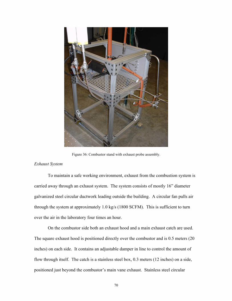
Figure 36: Combustor stand with exhaust probe assembly.

Exhaust System

To maintain a safe working environment, exhaust from the combustion system is

carried away through an exhaust system. The system consists of mostly 16” diameter

galvanized steel circular ductwork leading outside the building. A circular fan pulls air

through the system at approximately 1.0 kg/s (1800 SCFM). This is sufficient to turn

over the air in the laboratory four times an hour.

On the combustor side both an exhaust hood and a main exhaust catch are used.

The square exhaust hood is positioned directly over the combustor and is 0.5 meters (20

inches) on each side. It contains an adjustable damper in line to control the amount of

flow through itself. The catch is a stainless steel box, 0.3 meters (12 inches) on a side,

positioned just beyond the combustor’s main vane exhaust. Stainless steel circular

70

ductwork, 12” in diameter connects the box to the main line. The exhaust box contains

several closable windows enabling optical access to the combustor.

Laser Diagnostic System

Innovative Scientific Solutions Incorporated (ISSI) designed and installed the

advanced laser diagnostic system. As mentioned previously, this system enables the

AFIT small-scale combustion facility to conduct instantaneous Raman, PIV, PLIF, LII

and CARS diagnostics. The system is mounted on several movable optical breadboard

tables located around the combustor. The system operates free of excess clutter thanks to

the Unistrut frame.

The major components of the laser diagnostic system include:

• A dual-pulsed Nd:YAG laser that at 800mJ at 532nm wavelength produced by

Spectra Physics.

• A pulse stretcher and two ICCD cameras with a 5.0 ns gate.

• Various optics, filters and lenses as appropriate to the diagnostic techniques.

• A rail and traverse system for location of the appropriate optics and cameras.

• A Continuum ND600 narrowband dye laser with frequency doubler.

• A broadband dye laser created by ISSI

• A computer system with the associated control and analysis software.

71

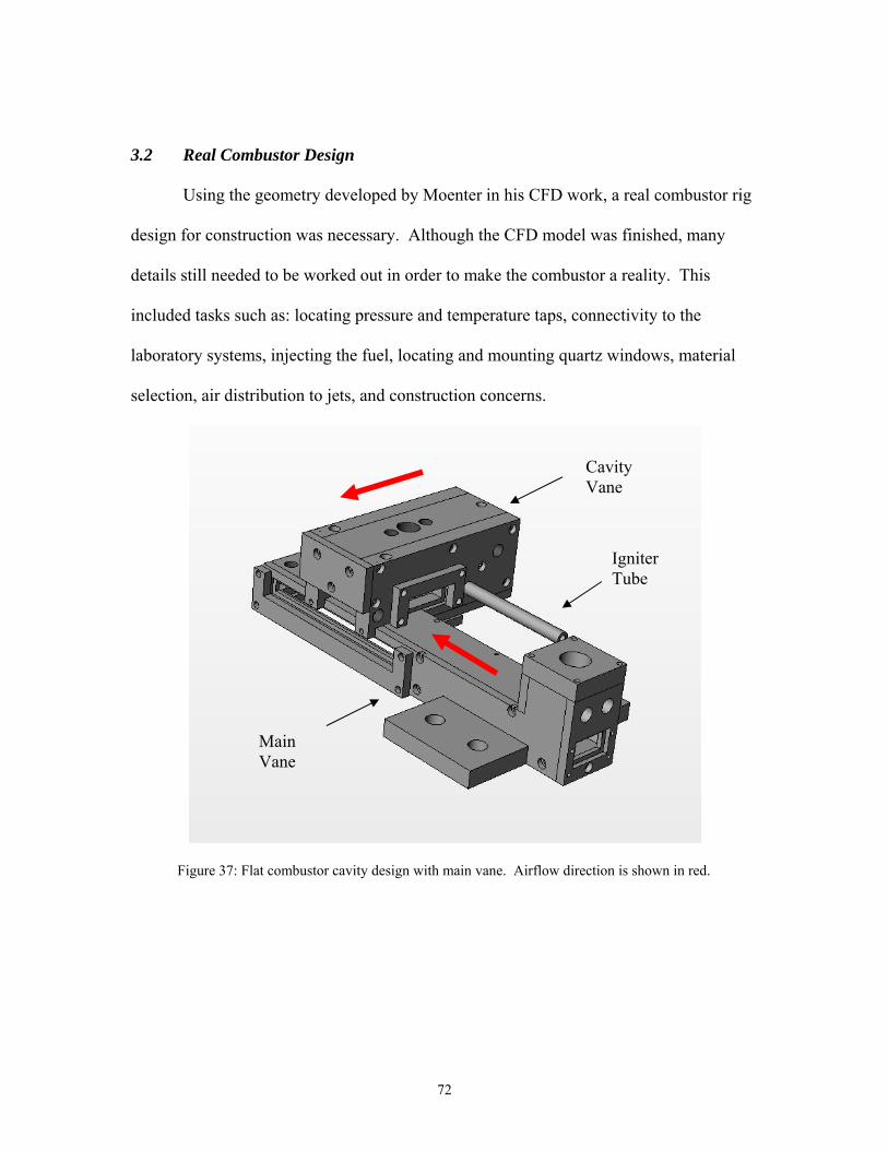
3.2 Real Combustor Design

Using the geometry developed by Moenter in his CFD work, a real combustor rig

design for construction was necessary. Although the CFD model was finished, many

details still needed to be worked out in order to make the combustor a reality. This

included tasks such as: locating pressure and temperature taps, connectivity to the

laboratory systems, injecting the fuel, locating and mounting quartz windows, material

selection, air distribution to jets, and construction concerns.

Cavity Vane

Igniter Tube

Main Vane

Figure 37: Flat combustor cavity design with main vane. Airflow direction is shown in red.

72

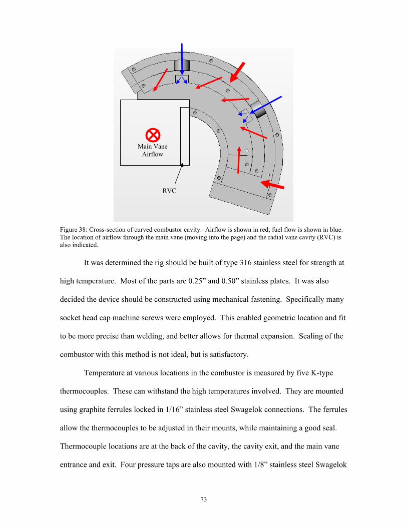
Main Vane Airflow

RVC

Figure 38: Cross-section of curved combustor cavity. Airflow is shown in red; fuel flow is shown in blue. The location of airflow through the main vane (moving into the page) and the radial vane cavity (RVC) is also indicated.

It was determined the rig should be built of type 316 stainless steel for strength at

high temperature. Most of the parts are 0.25” and 0.50” stainless plates. It was also

decided the device should be constructed using mechanical fastening. Specifically many

socket head cap machine screws were employed. This enabled geometric location and fit

to be more precise than welding, and better allows for thermal expansion. Sealing of the

combustor with this method is not ideal, but is satisfactory.

Temperature at various locations in the combustor is measured by five K-type

thermocouples. These can withstand the high temperatures involved. They are mounted

using graphite ferrules locked in 1/16” stainless steel Swagelok connections. The ferrules

allow the thermocouples to be adjusted in their mounts, while maintaining a good seal.

Thermocouple locations are at the back of the cavity, the cavity exit, and the main vane

entrance and exit. Four pressure taps are also mounted with 1/8” stainless steel Swagelok

73

connections. Several Dwyer 682 series pressure transducers and two Dwyer 655 series

differential pressure transducers read pressure from these taps. Pressure taps are located

directly across from all thermocouple locations.

Quartz windows, 0.3175 cm (1/8”) in thickness, are mounted on the combustor in

many locations to allow access to laser diagnostics. The mount is provided by recessed

cavities in the combustor that locate the quartz while leaving 1/16” all around it to

provide for differences in thermal expansion. The quartz is then sandwiched into position

between the recessed cavity and another piece of stainless steel. The plate is compressed

on the quartz using a screw-mounted spring. The window seals using a layer of high

temperature Unifrax ceramic paper, 0.159 cm (1/16”) in thickness.

As mentioned previously, two combustor rigs were developed; one uses a curved

cavity geometry, the other a flat geometry. Testing and comparison of both rigs will

allow for the isolation of the centrifugal effects on the combustor. The two rigs use the

exact same main vane geometry, so the cavities are interchangeable with the same main

vane section. This section cantilevers off the laboratories combustion stand to allow for

maximum access.

Windows are located in the main vane across from and perpendicularly below the

RVC cavity. Another window is located perpendicular to both the RVC windows, at the

main vane entrance. Immediately across from this window is the main vane exhaust,

open to the atmosphere. Windows in the laboratory’s exhaust vent will allow for full

access to the RVC cavity by laser diagnostics. The flat rig has two windows across from

each other in the cavity section and one perpendicular to these windows on the bottom.

This allows for a variety of diagnostic techniques to be employed in the cavity.

74

Fuel is injected into the rig using two Goodrich 46817-33 pressure-atomizing

nozzles. The nozzles spray at a full cone angle of 80° and have a 0.3 flow number. This

differs from the cone angles of the Moenter CFD models.

Ignition of the rig is in the cavity section, upstream of the first fuel injection point.

A 3/8” stainless steel tube is welded to the cavity sidewall, and connected to the ethylene

torch ignition system previously described. Fuel from the atomizers collects on the

cavity’s sidewall, and thus this torch location may be considered the most ideal place for

ignition.

75

IV. Results and Discussion

The implementation of the facility design, along with innovative solutions developed

during construction has resulted in a practical and flexible laboratory for AFIT to conduct

combustion research. This was made possible by the selection of materials, systems and

parts useful in any one of a variety of combustion research projects. The major

capabilities of this design and the flexibility of the laboratory will be discussed in this

section.

The combustor stand is oversized for the sectional combustor rigs for the purpose of

future experiments. The use of the 80/20 extruded aluminum system provides plenty of

strength for much larger systems. The particular combustion experiment can be designed

to bolt onto the stand in a variety of ways through the use of the channels and T-nuts that

are part of the 80/20 design. The track system not only provides for easy calibration, but

also variable positioning as the experiment demands. The stand is also removable and

exchangeable. All connections to the stand are Swagelok compression fittings and thus

easily exchangeable or replaceable when necessary. Hot connections are treated with a

nickel based anti-seize lubricant to ensure repeatable use and exchange.

The exhaust system provides significantly more airflow than is necessary for the UCC

sectional rig experiments. The exhaust’s ability to turn over the volume of room air

several times an hour will ensure safety of those conducting experiments on systems

much larger than those currently planned. The use of both an exhaust hood and a

horizontal catch will also allow open and varying exhaust orientations such as in the

planned UCC experiment.

76

The positioning of the stand and the exhaust capabilities make open flame

experiments practical. This is necessary for a combustion facility as operating only

enclosed experiments significantly reduces the amount of research that can be done.

This capability opens up a wide variety of possible uses including rocket motors, burners

and other open flame phenomena.

The use of two combustor rig airlines of differing sizes was necessary to research of the

UCC. It also allows flexibility in future experiments where two independently controlled

airlines are needed. As mentioned previously the main line is intended to provide up to

0.12 kg/s (200 SCFM), and the secondary 0.03 kg/s (60 SCFM) of air. Based on these

values and the possible flow rates of the fuel pump, equivalence ratios for JP-8 can be

obtained for maximum airflow. The main line ranges from 0.0018 to 1.3 and the

secondary can vary from 0.0061 to 4.3. The variable heating of this air up to 530K

(500°F), or 670K (750°F) without the use of the flexible connection hoses, is also useful

for a range of experimental conditions.

The use of the California Analytical Instruments gas analyzer and supporting

hardware allows the laboratory to conform to the testing standards laid out in the SAE

ARP 1256. The analyzer’s uncertainty and drift are within acceptable ranges of the

standards. The heated emissions transport line and heated filter are part of the CAI

system. The heated valves and lines provided by the laboratory design near the probe,

and the hot oil system also allows these standards to be maintained. This makes the

facility fully capable of gas emission sampling up to standard.

The computerized control of the lab and use of the National Instruments hardware

and LabView software is another advantage of the system. The NI products are

77

commonly used for data acquisition in a variety of laboratories across the country. The

LabView graphical programming software is relatively easy to learn, use and manipulate.

As the majority of the systems are based on computer control, setup for a differing

experiment may be accomplished simply by software modification. Use of computer-

controlled valves allows the lab operation to be literally programmed as desired. Remote

ignition, purging and emergency shutoff allow involved experiments to be conducted,

with little concern for potentially complex laboratory operations. Finally, all of the

associated control hardware has much more connectivity than is currently being used.

This means the addition of more systems to the laboratory would be easily accomplished.

The capabilities of the base laboratory systems are enhanced greatly by the

installation of the advanced laser diagnostics system. This system will allow any

knowledgeable user of the laboratory to conduct state-of-the-art combustion research.

The accessibility provided by the combustor stand and exhaust design will allow laser use

in almost any orientation. The system will allow studies of the flame and exhaust in

regards to point and planar studies of species concentration, temperature, soot location,

flame location, and velocity fields.

78

V. Conclusions

5.1 Overview of Project

The AFIT small-scale combustion facility is complete and its first experiment

designed and built. Starting with existing design and construction of much of the facility

by Dittman, new designs and specifics for the completion of the facility were developed.

Purchasing of parts and construction was then completed. A design for two sectional

combustor rigs, one with a curved cavity and one flat were created based on the CFD

work of Moenter. The flat rig design was constructed. It will provide the inaugural test

in the laboratory. Documentation and organization of the laboratory for future

modification and operation were also completed. Finally, an accessible but detailed

investigation into the basics of the combustion laser diagnostics available for use in this

laboratory was conducted.

The facility gives future researchers the ability to perform open flame or

contained combustion experiments with great flexibility. Two independently controlled

air lines provide heated air at different flow rates. The air can be delivered at up to 530 K

(500°F) at 0.12 kg/s (200 SCFM) for the large line and 0.03 kg/s (60 SCFM) for the

smaller. The air is delivered at nearly atmospheric pressure. Two syringe pumps

continuously provide liquid fuel at up to 5.67 mL/s.

Emissions sampling and testing is provided within standards as defined by SAE

ARP 1256. Use of oil cooling and electrical heating maintains sample temperature as

prescribed during transport to equipment meeting testing standards. Thus, the results of

any emissions tests conducted by the facility are given credibility. Additional data is

provided by several systems. The simplest of these are strategically placed

79

thermocouples and pressure taps for recording of point temperature and pressure values.

A humidity transmitter also gives water content of incoming rig air.

The installation of an advanced laser combustion diagnostics system will provide

a wealth of possibilities to the researcher. This system will be capable of conducting

instantaneous Raman, Raman spectroscopy, CARS, PLIF and LII measurements. These

allow both point and planar measurements of species concentration; temperature,

velocity, soot location and combustion location to be assessed.

The facility is centrally controlled and data is automatically taken through a

computer control station. Routing of electrical control and information systems through

this station provides for safe and simple control of the laboratory. Thus, the researcher

can concentrate on the experiment itself while easily accessing controls from a single

location. This station also uses data acquisition software and hardware enabling

modification for a variety of tests.

5.2 Future Work and Recommendations

Several steps will be necessary to bring the system fully online. Minor parts for

the completion of the combustor stand, installation of the gases and construction of the

flat UCC rig are currently on order but have not yet arrived. Construction of the laser

system and the exhaust system is currently being completed. A live fire has not been

conducted and adjustments may have to be made as a result of the first few tests. This

will likely result in a more detailed operating checklist as well. When firm dates for

testing are established the ordering of calibration, span and fuel gases along with JP-8

must be completed.

80

All aspects of the system that are fully in place have been tested and are prepared

for use in research on the UCC flat sectional combustor rig. All valve control systems

are operating correctly, and the rig air system has been validated. Pressures and

temperature readings are reasonable, as is data from the gas analyzer. Remote range

selection on the analyzer by the computer station operates correctly. Signal readings

from all other devices are also working correctly. The emissions transport system and

combustor stand equipment is operating properly.

It is suggested research begins with a study of the UCC flat sectional rig’s exhaust

by use of the emissions probe and gas analyzer. The laboratory is currently prepared for

this configuration and the rig will be soon completed. Running this test will enable

validation of the system in an actual experiment, and provide good data for investigation

of the UCC. It is also suggested that OH PLIF studies of a calibration device (such as a

Hankin burner) be conducted to validate the laser diagnostic system. These two

experiments will give the facility and researcher a good grounding for future work.

81

Appendix A: System Technical Information

Table 4: Wiring code for NI SCXI 1100 DAQ measurement and control system.

SCXI 1100 Slot Location NI Module

NI Terminal Block NI Channel #

Enclosure Terminal Block Connection # Polarity

Instrument Connection # Description of Instrument Connection

1 SCXI 1102 SCXI1303 CH0+ ETB A - 1 + CAI TB3-11 SCXI 1102 SCXI1303 CH0- ETB A - 2 - CAI TB3-2

ETB A - 3 Ground1 SCXI 1102 SCXI1303 CH1+ ETB A - 4 + CAI TB3-7 1 SCXI 1102 SCXI1303 CH1- ETB A - 5 - CAI TB3-8

ETB A - 6 Ground1 SCXI 1102 SCXI1303 CH2+ ETB A - 7 + CAI TB3-181 SCXI 1102 SCXI1303 CH2- ETB A - 8 - CAI TB3-19

ETB A - 9 Ground1 SCXI 1102 SCXI1303 CH3+ ETB A - 10 + CAI TB3-241 SCXI 1102 SCXI1303 CH3- ETB A - 11 - CAI TB3-25

ETB A - 12 Ground1 SCXI 1102 SCXI1303 CH4+ ETB A - 13 + CAI TB3-27 1 SCXI 1102 SCXI1303 CH4- ETB A - 14 - CAI TB3-28

ETB A - 15 Ground1 SCXI 1102 SCXI1303 CH5+ ETB A - 16 + CAI TB3-371 SCXI 1102 SCXI1303 CH5- ETB A - 17 - CAI TB3-38

ETB A - 18 Ground1 SCXI 1102 SCXI1303 CH6+ ETB A - 19 + CAI TB3-451 SCXI 1102 SCXI1303 CH6- ETB A - 20 - CAI TB3-46

ETB A - 21 Ground1 SCXI 1102 SCXI1303 CH7+ ETB A - 22 + CAI TB3-531 SCXI 1102 SCXI1303 CH7- ETB A - 23 - CAI TB3-54

ETB A - 24 Ground1 SCXI 1102 SCXI1303 CH25+ ETB A - 29 + 1+1 SCXI 1102 SCXI1303 CH25- ETB A - 30 - 1-

Viasala Dewpoint Transmitter Output (4-20mA DC)

California Analytical Instruments (CAI) THC Analyzer Output (4-20mA DC)

THC Oven Temperature (1 mV/°C)

NOx Analyzer Output (4-20mA DC)

NOx Conv Temperature (10 mV/°C)

NOx Oven Temperature (10 mV/°C)

CO2 Analyzer Output (4-20mA DC)

CO Analyzer Output (4-20mA DC)

O2 Analyzer Output (4-20mA DC)

82

Table 4: Wiring code for NI SCXI 1100 DAQ measurement and control system. (continued)

SCXI 1100 Slot Location NI Module

NI Terminal Block NI Channel #

Enclosure Terminal Block Connection # Polarity

Instrument Connection # Description of Instrument Connection

2 SCXI 1102 SCXI1303 CH0+ ETB A - 27 + PT 12 SCXI 1102 SCXI1303 CH0- ETB A - 28 - -12 SCXI 1102 SCXI1303 CH1+ ETB C -1 + Ch2 SCXI 1102 SCXI1303 CH1- ETB C - 1 - Al2 SCXI 1102 SCXI1303 CH2+ ETB A - 31 + PT 22 SCXI 1102 SCXI1303 CH2- ETB A - 32 - -22 SCXI 1102 SCXI1303 CH3+ ETB A - 33 + TS1 -2 SCXI 1102 SCXI1303 CH3- ETB A - 34 - TS2 4-2 SCXI 1102 SCXI1303 CH4+ ETB A - 35 + 2A+2 SCXI 1102 SCXI1303 CH4- ETB A - 36 - 2B-2 SCXI 1102 SCXI1303 CH5+ ETB A - 37 + 142 SCXI 1102 SCXI1303 CH5- ETB A - 38 - 152 SCXI 1102 SCXI1303 CH6+ ETB A - 39 + PT 42 SCXI 1102 SCXI1303 CH6- ETB A - 40 - -42 SCXI 1102 SCXI1303 CH7+ ETB C - 2 + Ch2 SCXI 1102 SCXI1303 CH7- ETB C - 2 - Al2 SCXI 1102 SCXI1303 CH8+ ETB A - 43 + PT 32 SCXI 1102 SCXI1303 CH8- ETB A - 44 - -32 SCXI 1102 SCXI1303 CH9+ ETB C - 3 + Ch2 SCXI 1102 SCXI1303 CH9- ETB C - 3 - Al2 SCXI 1102 SCXI1303 CH10+ ETB A - 47 + PT 62 SCXI 1102 SCXI1303 CH10- ETB A - 48 - -62 SCXI 1102 SCXI1303 CH11+ ETB A - 49 + TS1 -2 SCXI 1102 SCXI1303 CH11- ETB A - 50 - TS2 4-2 SCXI 1102 SCXI1303 CH12+ ETB A - 51 + 2A+2 SCXI 1102 SCXI1303 CH12- ETB A - 52 - 2B-2 SCXI 1102 SCXI1303 CH13+ ETB A - 53 + 142 SCXI 1102 SCXI1303 CH13- ETB A - 54 - 152 SCXI 1102 SCXI1303 CH14+ ETB A - 55 + PT52 SCXI 1102 SCXI1303 CH14- ETB A - 56 - -52 SCXI 1102 SCXI1303 CH15+ ETB C - 4 + Ch2 SCXI 1102 SCXI1303 CH15- ETB C - 4 - Al2 SCXI 1102 SCXI1303 CH16+ ETB A - 59 + PT82 SCXI 1102 SCXI1303 CH16- ETB A - 60 - -82 SCXI 1102 SCXI1303 CH17+ ETB C - 5 + Ch2 SCXI 1102 SCXI1303 CH17- ETB C - 5 - Al2 SCXI 1102 SCXI1303 CH18+ ETB C - 6 + Ch2 SCXI 1102 SCXI1303 CH18- ETB C - 6 - Al2 SCXI 1102 SCXI1303 CH19+ ETB A - 65 + PT92 SCXI 1102 SCXI1303 CH19- ETB A - 66 - -92 SCXI 1102 SCXI1303 CH24+ ETB C - 8 + Ch2 SCXI 1102 SCXI1303 CH24- ETB C - 8 - Al2 SCXI 1102 SCXI1303 CH25+ ETB C - 9 + Ch2 SCXI 1102 SCXI1303 CH25- ETB C - 9 - Al2 SCXI 1102 SCXI1303 CH26+ ETB C - 10 + Ch2 SCXI 1102 SCXI1303 CH26- ETB C - 10 - Al2 SCXI 1102 SCXI1303 CH29+ ETB A - 67 + Gaseous Fuel Flow (for future use)2 SCXI 1102 SCXI1303 CH29- ETB A - 68 -2 SCXI 1102 SCXI1303 CH30+ ETB A - 69 + PT72 SCXI 1102 SCXI1303 CH30- ETB A - 70 - -72 SCXI 1102 SCXI1303 CH31+ ETB C - 7 + Ch2 SCXI 1102 SCXI1303 CH31- ETB C - 7 - Al

(PT 5) Secondary Line pressure difference across combustor, Pressure Transducer Box 1 (4-20mA DC)

(TC 8) Main Line temperature at combustor exit (K Type TC)(TC 9) Secondary Line temperature at combustor inlet (K Type TC)(TC 10) Cavity back wall temperature (K Type TC)

(TC 4) Secondary Line temperature at combustor inlet (K Type TC)

(TC 3) Secondary Line temperature before dome loader (K Type TC)(PT 6) Secondary Line Pressure at combustor inlet, Pressure Transducer Box 2 (4-20mA DC)

(TC 2) Main Line temperature at combustor inlet (K Type TC)

Main Line temperature from heater controller UT420 (4-20mA DC)

Secondary Line temperature from heater controller UT420 (4-20mA DC)

(PT 4) Main Line pressure difference across combustor, Pressure Transducer Box 1 (4-20mA DC)

(PT 1) Main Line pressure before dome loader, Pressure Tranducer Box 1 (4-20mA DC)(TC 1) Main Line temperature before dome loader (K Type TC)(PT 2) Main Line Pressure at combustor inlet, Pressure Transducer Box 1 (4-20mA DC)Main Line temperature from Fox Box 1 (4-20mA DC)Main Line Flow from 2404 PID Controller (4-20mA DC) (Retransmitted from Fox Box 1)

Secondary Line temperature from Fox Box 2 (4-20mA DC)Secondary Line Flow from 2404 PID Controller (4-20mA DC) (Retransmitted from Fox Box 2)

(PT 3) Secondary Line pressure before dome loader, Pressure Transducer Box 1 (4-20mA DC)

( PT 8) Liquid Fuel Pressure, Pressure Transducer Box 2 (4-20mA DC)(TC 5) Liquid Fuel Temperature from thermocouple (K Type TC)(TC 6) Oil Temperature from thermocouple (K Type TC)(PT 9) Ambient pressure, Pressure Transducer Box 2 (4-20mA DC)

(PT 7) Gaseous Fuel Pressure, Pressure Transducer Box 2 (4-20mA DC)(TC 7) Gaseous Fuel Temperature from thermocouple (K-Type TC)

83

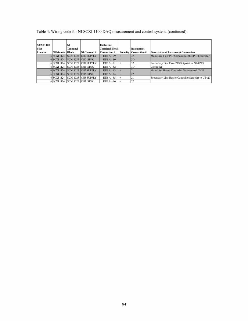
Table 4: Wiring code for NI SCXI 1100 DAQ measurement and control system. (continued) SCXI 1100 Slot Location NI Module

NI Terminal Block NI Channel #

Enclosure Terminal Block Connection # Polarity

Instrument Connection # Description of Instrument Connection

6 SCXI 1124 SCXI 1325 CH0 SUPPLY ETB A - 79 + 3A6 SCXI 1124 SCXI 1325 CH0 ISINK ETB A - 80 - 3D6 SCXI 1124 SCXI 1325 CH1 SUPPLY ETB A - 81 + 3A6 SCXI 1124 SCXI 1325 CH1 ISINK ETB A - 82 - 3D6 SCXI 1124 SCXI 1325 CH2 SUPPLY ETB A - 83 + 216 SCXI 1124 SCXI 1325 CH2 ISINK ETB A - 84 - 226 SCXI 1124 SCXI 1325 CH3 SUPPLY ETB A - 85 + 216 SCXI 1124 SCXI 1325 CH3 ISINK ETB A - 86 - 22

Secondary Line Heater Controller Setpoint to UT420

Main Line Heater Controller Setpoint to UT420

Secondary Line Flow PID Setpoint to 2404 PID Controller

Main Line Flow PID Setpoint to 2404 PID Controller

84

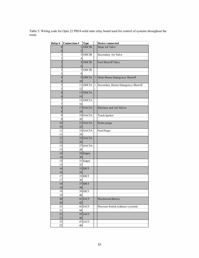
Table 5: Wiring code for Opto 22 PB24 solid state relay board used for control of systems throughout the room.

Relay # Connection # Type Device connected0 1 ODC5R Main Air Valve0 21 3 ODC5R Secondary Air Valve1 42 5 ODC5R Fuel Shutoff Valve2 63 7 ODC5R3 84 9 ODC5A + Main Heater Emergency Shutoff4 10 -5 11 ODC5A + Secondary Heater Emergency Shutoff5 12 -6 13 ODC5A6 147 15 ODC5A7 168 17 OAC5A Ethylene and Air Valves8 189 19 OAC5A Torch Ignitor9 20

10 21 OAC5A Probe purge10 2211 23 OAC5A Fuel Purge11 2412 25 OAC5A12 2613 27 OAC5A13 2814 29 Empty14 3015 31 Empty15 3216 33 IDC516 3417 35 IDC517 3618 37 IDC518 3819 39 IDC519 4020 41 IAC5 Mushroom Button20 4221 43 IAC5 Pressure Switch (exhaust system)21 4422 45 IAC522 4623 47 IAC523 48

85

Table 6: Wiring and digital channel code for Opto 22 G4PB24 optically isolated solid-state relay board used for controlling range selection on the raw emissions test bench.

Opto 22 G4PB24 Connection #

Enclosure Terminal Block Connection #

CAI Analyzer Rack Connection # CAI Control Description

50 Pin Connector Line #

DAQ Pad-6508 Port and Channel

46 ETB B - 1 58 Oxygen Range 3 (0-25%) 3 CPC(8):644 ETB B -2 57 Oxygen Range 2 (0-10%) 5 CPC(8):542 ETB B - 3 56 Oxygen Range 1 (0-5%) 7 CPC(8):4

41,43,45 ETB B - 4 59 Oxygen Remote 7,5,3 CPC(8):4-640 ETB B - 5 49 CO Range 2 (0-1%) 9 CPC(8):338 ETB B - 6 48 CO Range 1 (0-2k ppm) 11 CPC(8):2

37,39 ETB B - 7 51 CO Remote 11,9 CPC(8):2-336 ETB B - 8 41 CO2 Range 2 (0-20%) 13 CPC(8):134 ETB B - 9 40 CO2 Range 1 (0-5%) 15 CPC(8):0

33,35 ETB B - 10 42 CO2 Remote 15,13 CPC(8):0-126 ETB B - 11 34 NOx Range 5 (0-3k ppm) 23 CPB(7):424 ETB B - 12 33 NOx Range 4 (0-1k ppm) 25 CPB(7):322 ETB B - 13 32 NOx Range 3 (0-300 ppm) 27 CPB(7):220 ETB B - 14 62 NOx Range 2 (0-100 ppm) 29 CPB(7):118 ETB B - 15 61 NOx Range 1 (0-30 ppm) 31 CPB(7):0

17,19,21,23,25 ETB B - 16 35 NOx Remote 31,29,27,25,23 CPB(7):0-414 ETB B - 17 68 THC Range 7 (0-10k ppm) 35 CPA(6):612 ETB B - 18 15 THC Range 6 (0-3k ppm) 37 CPA(6):510 ETB B - 19 14 THC Range 5 (0-1k ppm) 39 CPA(6):48 ETB B - 20 13 THC Range 4 (0-300 ppm) 41 CPA(6):36 ETB B - 21 67 THC Range 3 (0-100 ppm) 43 CPA(6):24 ETB B - 22 66 THC Range 2 (0-30 ppm) 45 CPA(6):12 ETB B - 23 69 THC Range 1 (0-10 ppm) 47 CPA(6):0

1,3,5,7,9,11,13 ETB B - 24 16 THC Remote 47,45,43,39,37,35 CPA(6):0-6

86

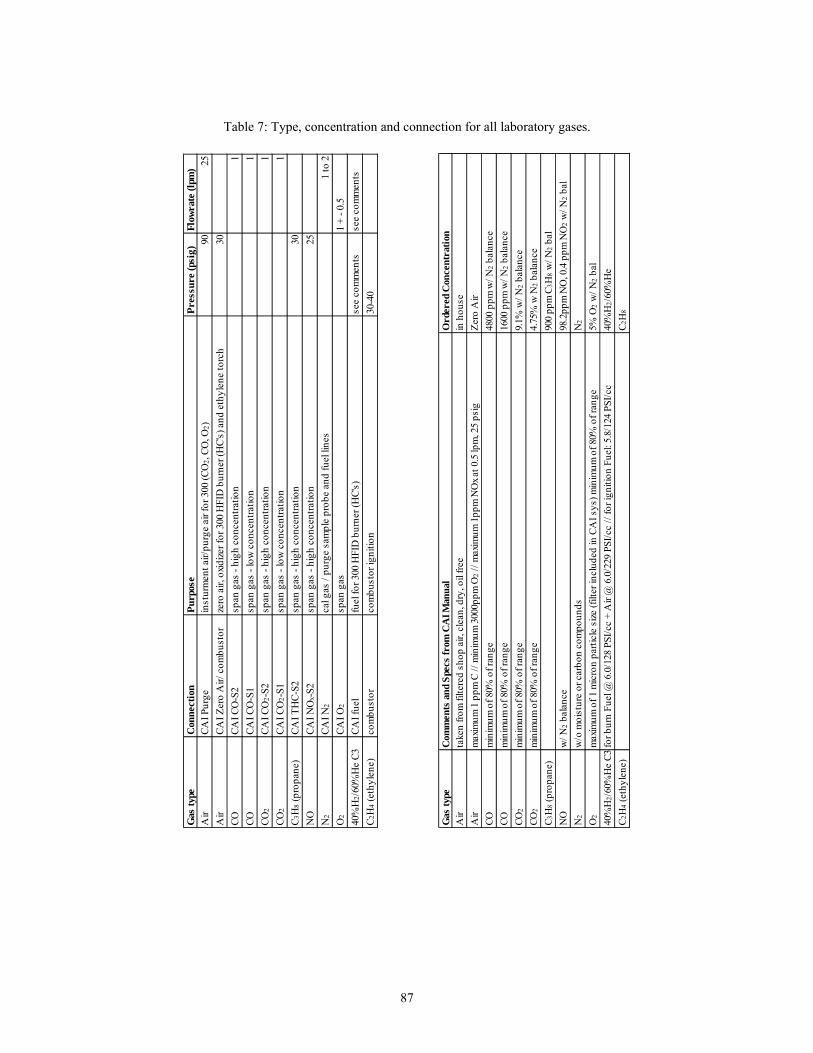
Table 7: Type, concentration and connection for all laboratory gases.

Gas

type

Con

nect

ion

Purp

ose

Pres

sure

(psi

g)Fl

owra

te (l

pm)

Air

CAI P

urge

inst

urm

ent a

ir/pu

rge

air f

or 3

00 (C

O2,

CO, O

2)9

Air

CAI Z

ero

Air/

com

bust

orze

ro a

ir, o

xidize

r for

300

HFI

D b

urne

r (H

C's)

and

eth

ylen

e to

rch

30CO

CAI C

O-S

2sp

an g

as -

high

con

cent

ratio

n1

COCA

I CO

-S1

span

gas

- lo

w c

once

ntra

tion

1CO

2CA

I CO

2-S2

span

gas

- hi

gh c

once

ntra

tion

1CO

2CA

I CO

2-S1

span

gas

- lo

w c

once

ntra

tion

1C 3

H8 (

prop

ane)

CAI T

HC-

S2sp

an g

as -

high

con

cent

ratio

n30

NO

CAI N

Ox-S

2sp

an g

as -

high

con

cent

ratio

n25

N2

CAI N

2ca

l gas

/ pu

rge

sam

ple

prob

e an

d fu

el li

nes

1 to

2O

2CA

I O2

span

gas

1 +

- 0.5

40%

H2/

60%

He

C3CA

I fue

lfu

el fo

r 300

HFI

D b

urne

r (H

C's)

see

com

men

tsse

e co

mm

ents

C 2H

4 (et

hyle

ne)

com

bust

orco

mbu

stor

igni

tion

30-4

0

025

Gas

type

Com

men

ts a

nd S

pecs

from

CA

I Man

ual

Ord

ered

Con

cent

ratio

nA

irta

ken

from

filte

red

shop

air,

cle

an, d

ry, o

il fre

ein

hou

seA

irm

axim

um 1

ppm

C //

min

imum

300

0ppm

O2 /

/ max

imum

1pp

m N

Ox a

t 0.5

lpm

, 25

psig

Zero

Air

COm

inim

um o

f 80%

of r

ange

4800

ppm

w/ N

2 bal

ance

COm

inim

um o

f 80%

of r

ange

1600

ppm

w/ N

2 bal

ance

CO2

min

imum

of 8

0% o

f ran

ge9.

1% w

/ N2 b

alan

ceCO

2m

inim

um o

f 80%

of r

ange

4.75

% w

N2 b

alan

ceC 3

H8 (

prop

ane)

900

ppm

C3H

8 w/ N

2 bal

NO

w/ N

2 bal

ance

98.2

ppm

NO

, 0.4

ppm

NO

2 w/ N

2 bal

N2

w/o

moi

stur

e or

car

bon

com

poun

dsN

2

O2

max

imum

of 1

mic

ron

parti

cle

size

(filt

er in

clud

ed in

CA

I sys

) min

imum

of 8

0% o

f ran

ge5%

O2 w

/ N2 b

al40

%H

2/60

%H

e C3

for b

urn

Fuel

@ 6

.0/1

28 P

SI/c

c +

Air

@ 6

.0/2

29 P

SI/c

c //

for i

gniti

on F

uel:

5.8/

124

PSI/c

c40

%H

2/60

%H

eC 2

H4 (

ethy

lene

)C 2

H8

87

Table 8: Compiled list of major equipment and technical data by system.

Air Heater Model Serial # Line Use Outlet Temp Power Limits

GaumerCS5F9N884YKWJ 05-11326 480V, 3 Phase

Heats main line combustor rig air

up to 538 °C (1000 F) 37.5 kW

GaumerC2P3N64M4KWJ 05-11326 480V, 3 Phase

Heats combustor rig air

up to 538 °C (1000 F) 12.3 kW

Current to Pressure Transmitter Model Serial # Range Use Accuracy Pressure Limits

Moore Industries IPT2 1725762

0.21-1.03 bar (3-15 psig)

Takes signal from process controller and converts to pressure value for the needle valves

±0.1% of output pressure

Supply pressure must be 5 psi greater than upper signal, 20 to 40 psi

Flow Meters Model Serial # Range Use Accuracy Pressure Limits

Fox Thermal Instruments FT2 W749 0-7.0 kg/min

Measure air flow in main line

±1% of reading

20.68 bar (300 psi)

FT3 W382 0-2.0 kg/min

Measure air flow in secondary line

±1% of reading

20.68 bar (300 psi)

Fuel Atomizers Model Serial # Press Loss Use Flow Number Pressure Limits

Goodrich

Peanut tip pressure atomizer 46817-33 n/a

6.89 bar (100 psi) at 0.0037 kg/s (0.5 lbm/min) of fuel

Filters fuel to pump and combustor 0.3 n/a

Fuel Filters Model Serial # Press Loss Use Filtration Pressure Limits

Mott

6610-.170-10 (10 micron) 6610-.170-40 (40 micron)

6066101-100 6066101-400 n/a

Filters fuel to pump and combustor

10 and 40 micron respectively n/a

88

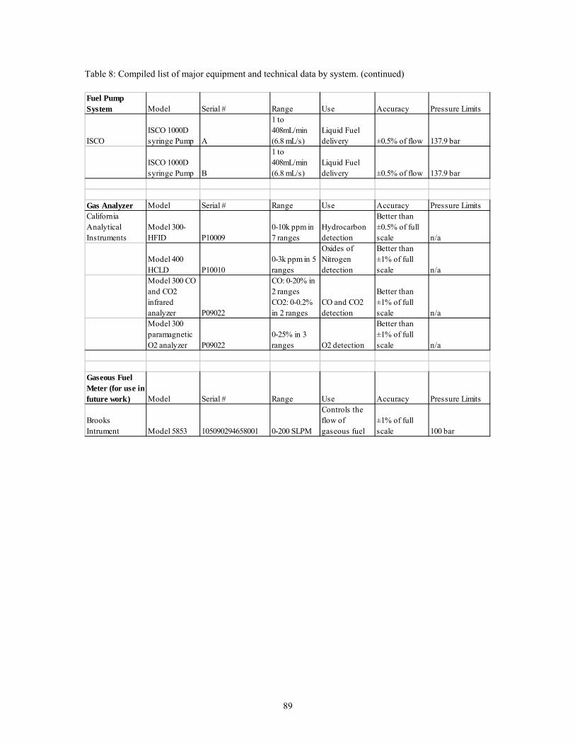
Table 8: Compiled list of major equipment and technical data by system. (continued) Fuel Pump System Model Serial # Range Use Accuracy Pressure Limits

ISCOISCO 1000D syringe Pump A

1 to 408mL/min (6.8 mL/s)

Liquid Fuel delivery ±0.5% of flow 137.9 bar

ISCO 1000D syringe Pump B

1 to 408mL/min (6.8 mL/s)

Liquid Fuel delivery ±0.5% of flow 137.9 bar

Gas Analyzer Model Serial # Range Use Accuracy Pressure LimitsCalifornia Analytical Instruments

Model 300-HFID P10009

0-10k ppm in 7 ranges

Hydrocarbon detection

Better than ±0.5% of full scale n/a

Model 400 HCLD P10010

0-3k ppm in 5 ranges

Oxides of Nitrogen detection

Better than ±1% of full scale n/a

Model 300 CO and CO2 infrared analyzer P09022

CO: 0-20% in 2 ranges CO2: 0-0.2% in 2 ranges

CO and CO2 detection

Better than ±1% of full scale n/a

Model 300 paramagnetic O2 analyzer P09022

0-25% in 3 ranges O2 detection

Better than ±1% of full scale n/a

Gaseous Fuel Meter (for use in future work) Model Serial # Range Use Accuracy Pressure Limits

Brooks Intrument Model 5853 105090294658001 0-200 SLPM

Controls the flow of gaseous fuel

±1% of full scale 100 bar

89

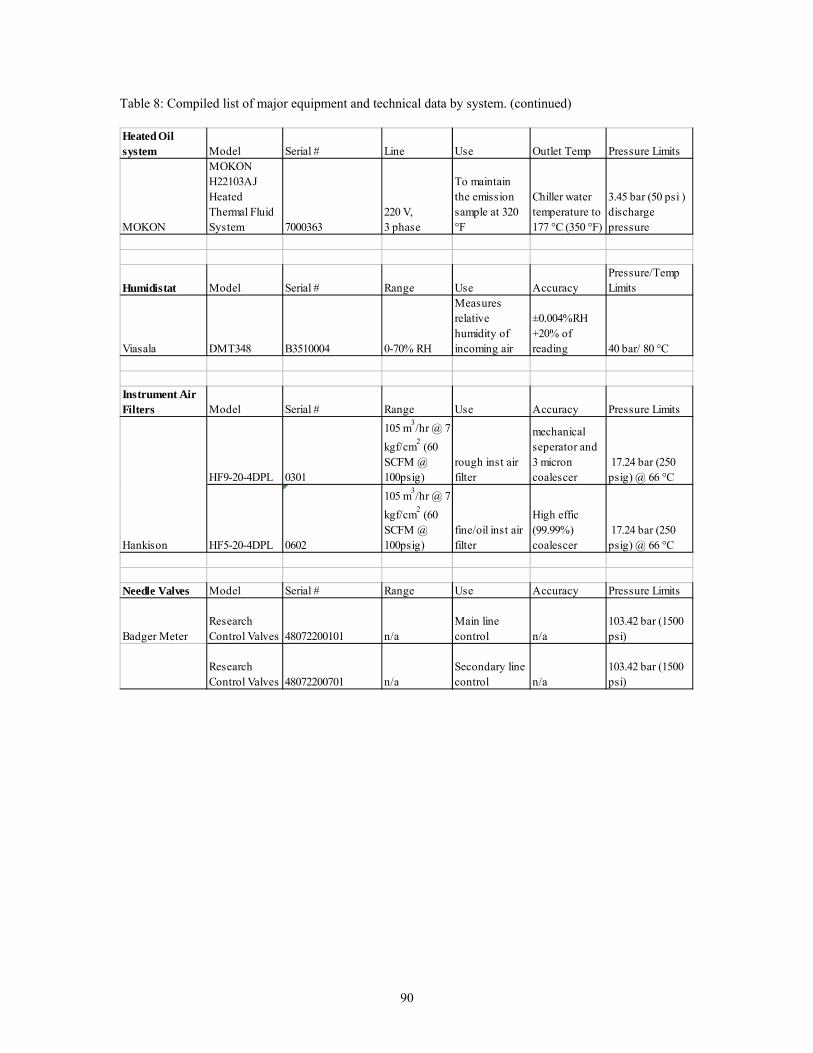
Table 8: Compiled list of major equipment and technical data by system. (continued) Heated Oil system Model Serial # Line Use Outlet Temp Pressure Limits

MOKON

MOKON H22103AJ Heated Thermal Fluid System 7000363

220 V, 3 phase

To maintain the emission sample at 320 °F

Chiller water temperature to 177 °C (350 °F)

3.45 bar (50 psi ) discharge pressure

Humidistat Model Serial # Range Use AccuracyPressure/Temp Limits

Viasala DMT348 B3510004 0-70% RH

Measures relative humidity of incoming air

±0.004%RH +20% of reading 40 bar/ 80 °C

Instrument Air Filters Model Serial # Range Use Accuracy Pressure Limits

HF9-20-4DPL 0301

105 m3/hr @ 7 kgf/cm2 (60 SCFM @ 100psig)

rough inst air filter

mechanical seperator and 3 micron coalescer

17.24 bar (250 psig) @ 66 °C

HF5-20-4DPL 0602

105 m3/hr @ 7 kgf/cm2 (60 SCFM @ 100psig)

fine/oil inst air filter

High effic (99.99%) coalescer

17.24 bar (250 psig) @ 66 °C

Needle Valves Model Serial # Range Use Accuracy Pressure Limits

Badger MeterResearch Control Valves 48072200101 n/a

Main line control n/a

103.42 bar (1500 psi)

Research Control Valves 48072200701 n/a

Secondary line control n/a

103.42 bar (1500 psi)

Hankison

90

Table 8: Compiled list of major equipment and technical data by system. (continued) Pneumatic Ball Valves Model Serial #

Actuation Pressure Use Temp Limits Pressure Limits

PC/S2S-3 n/a

5.52 to 8.27 bar (80 to 120 psig )

Fuel line shutoff n/a n/a

P0/B2F-12D1 P0/B2F-6D1 n/a

5.52 to 8.27 bar (80 to 120 psig )

Rig air shutoffs (main and sec) n/a n/a

PS/S2S-2TT n/a

5.52 to 8.27 bar (80 to 120 psig )

emissions line purge

182° C (360 °F) on seats and seals (Viton) n/a

PS/S2S-2TT n/a

5.52 to 8.27 bar (80 to 120 psig )

emissions line air feed

182 °C (360 °F) on seats and seals (Viton) n/a

Pressure Reducing Valve Model Serial # Range Use Accuracy Pressure Limits

CASHCO 1/2" NPT DA3 AA4098-001-060-27.58 bar (0-400 psig)

Change pressure in the main line n/a

27.58 bar (400 psi)

1/2" NPT DA3 AA4098-001-050-27.58 bar (0-400 psig)

Change pressure in the secondary line n/a

27.58 bar (400 psi)

UCI

91

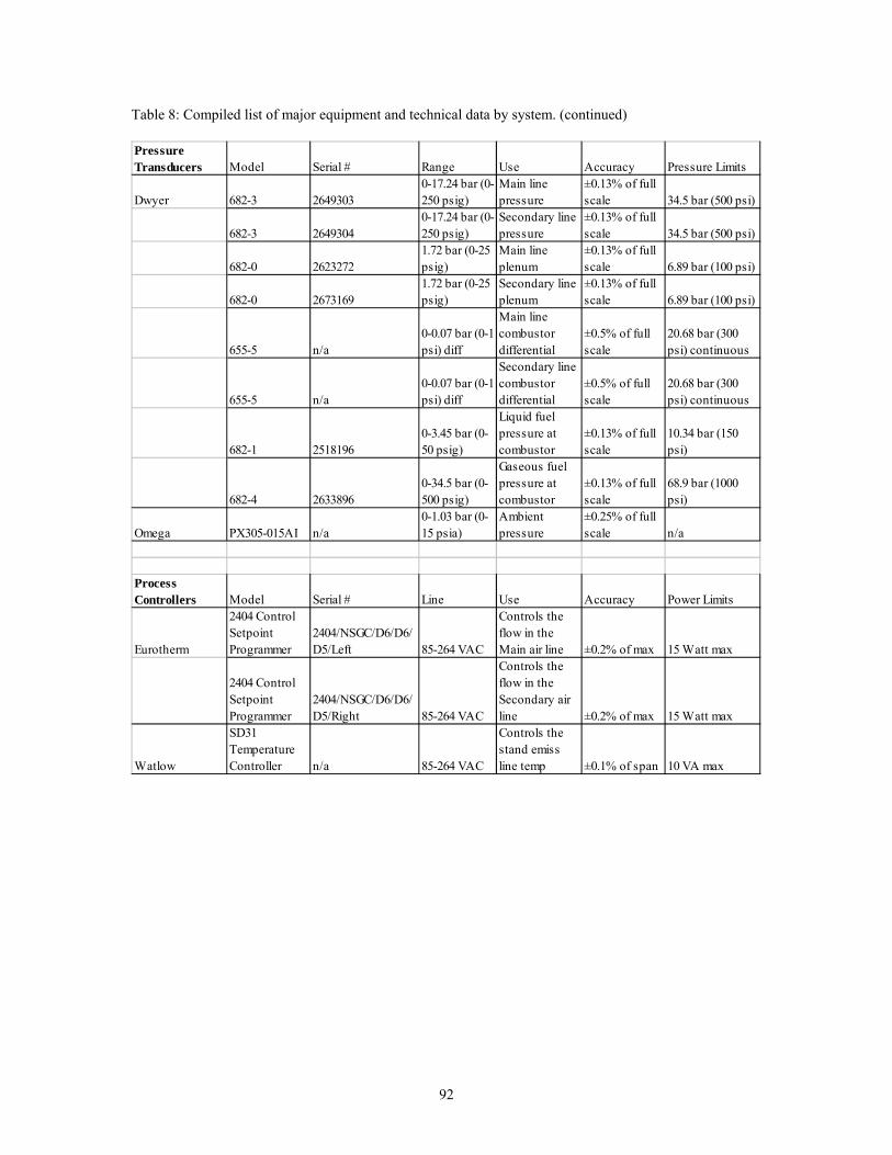
Table 8: Compiled list of major equipment and technical data by system. (continued) Pressure Transducers Model Serial # Range Use Accuracy Pressure Limits

Dwyer 682-3 26493030-17.24 bar (0-250 psig)

Main line pressure

±0.13% of full scale 34.5 bar (500 psi)

682-3 26493040-17.24 bar (0-250 psig)

Secondary line pressure

±0.13% of full scale 34.5 bar (500 psi)

682-0 26232721.72 bar (0-25 psig)

Main line plenum

±0.13% of full scale 6.89 bar (100 psi)

682-0 26731691.72 bar (0-25 psig)

Secondary line plenum

±0.13% of full scale 6.89 bar (100 psi)

655-5 n/a0-0.07 bar (0-1 psi) diff

Main line combustor differential

±0.5% of full scale

20.68 bar (300 psi) continuous

655-5 n/a0-0.07 bar (0-1 psi) diff

Secondary line combustor differential

±0.5% of full scale

20.68 bar (300 psi) continuous

682-1 25181960-3.45 bar (0-50 psig)

Liquid fuel pressure at combustor

±0.13% of full scale

10.34 bar (150 psi)

682-4 26338960-34.5 bar (0-500 psig)

Gaseous fuel pressure at combustor

±0.13% of full scale

68.9 bar (1000 psi)

Omega PX305-015AI n/a0-1.03 bar (0-15 psia)

Ambient pressure

±0.25% of full scale n/a

Process Controllers Model Serial # Line Use Accuracy Power Limits

Eurotherm

2404 Control Setpoint Programmer

2404/NSGC/D6/D6/D5/Left 85-264 VAC

Controls the flow in the Main air line ±0.2% of max 15 Watt max

2404 Control Setpoint Programmer

2404/NSGC/D6/D6/D5/Right 85-264 VAC

Controls the flow in the Secondary air line ±0.2% of max 15 Watt max

Watlow

SD31 Temperature Controller n/a 85-264 VAC

Controls the stand emiss line temp ±0.1% of span 10 VA max

92

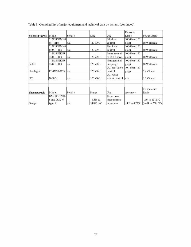
Table 8: Compiled list of major equipment and technical data by system. (continued)

Solenoid Valves Model Serial # Line UsePressure Limits Power Limits

71215SN2MN00H111P3 n/a 120 VAC

Ethylene control

10.34 bar (150 psig) 10 Watt max

71215SN2MN00N0C111P3 n/a 120 VAC

Torch air control

10.34 bar (150 psig) 10 Watt max

71295SN2KNJ1N0C111P3 n/a 120 VAC

Instrument air to UCI 3 ways

10.34 bar (150 psig) 10 Watt max

71295SN2KNJ1N0C111P3 n/a 120 VAC

Nitrogen fuel line purge

10.34 bar (150 psig) 10 Watt max

Hoerbiger PD43295-5733 n/a 120 VACUCI fuel valve control

10.14 bar (147 psig) 6.9 VA max

UCI N4S-D1 n/a 120 VACUCI rig air valves control n/a 6.0 VA max

Thermocouple Model Serial # Range Use AccuracyTemperature Limits

Omega

KMQSS-125U-6 and 062U-6 type K n/a

-6.458 to 54.886 mV

Temp point measurments in system ±4 F or 0.75%

-234 to 1372 °C ( -454 to 2501 °F)

Parker

93

94

Appendix B: Operational Checklist for System Startup

Make sure the “Equip” control switch at the control station is in the OFF position before system startup, this must be on after the VI is started To start up the laboratory equipment, turn ON the following:

1. Computer 2. Power switch on surge protector (powers DC supplies, SCXI 1100 and DAQPad

6508) 3. Instrument airline (note: another valve is located in Room 256)

a. Check pressure control valve to IPT2 reads 20-40 psi b. Check pressure control valve to other equipment reads 80 to 120 psi

4. ISCO fuel pump Next, do the following:

1. Open and START Combustion Lab VI on computer 2. Check that relays are responding to operation of VI controls

a. If this fails try stopping and restarting the VI and the DAQPad6508 b. If step 2a fails then restart computer

3. Turn ON the “Equip” switch and check proper operation of all valves a. Set all valves to OFF position before proceeding

4. Turn on California Analytical Instruments gas analyzer a. Check that the VI readings match the analyzer displays

Check the following:

1. Emissions temperature control is set to 340°F at control station 2. Emissions temperature control is set to 350°F at gas analyzer 3. Emissions filter is set to 200°F at gas analyzer 4. Pressure, temperature and humidistat readings are reasonable 5. Temperature setting for airline heaters is below 500°F

For ignition do the following:

1. Turn on the exhaust system 2. Turn ON the gases to combustor stand

a. Nitrogen b. Zero Air c. Ethylene (C2H4)

95

3. Turn ON the Mokon oil system – PROBE MUST BE IN DESIRED POSITION AND THERMOCOUPLE CONNECTED

a. Open bypass valve at heater b. Check temperature is set to 350°F c. Check discharge pressure is near but below 40 psi d. Ensure that chiller lines are open e. Power ON f. When fluid is to temperature, close bypass valve and recheck all settings g. Check temperature for probe oil temp is near 350°F in VI

4. Check that all valves are OFF at VI 5. Turn ON air heaters (temp setting must be below 500°F) 6. Set rig airline flow to rate for ignition 7. Open manual fuel line valve at combustor stand 8. Set fuel flow rate or pressure for ignition in VI 9. Turn ON probe purge at VI 10. Turn ON air valves at VI 11. Turn ON ethylene and air valves at VI 12. Turn ON ignition switch at VI 13. Check torch is ignited 14. Turn OFF ignition switch at VI 15. Turn ON fuel valve at VI 16. Turn ON fuel pump switch at VI 17. Check ignition has occurred 18. Turn OFF ethylene and air valves 19. Change air and fuel flow to desired settings 20. Proceed with experiment

Bibliography

AIAA Optical Diagnostics Reference Sheet, AIAA website, 23 January 2006. www.aiaa.org/tc/amt/techniques.html

Anisko, J. (2006). Numerical investigation of cavity-vane interactions within the ultra compact combustor. (Master's thesis, Graduate School of Engineering, Air Force Institute of Technology (AU), Wright-Patterson AFB OH, March 2006). (AFIT/GAE/ENY/06-M01)

Anthenien, R. A., Mantz, R. A., Roquemore, W. M., & Sturgess, G. (2001). Experimental results for a novel, high swirl, ultra compact combustor for gas turbine engines. 2nd Joint Meeting of the United States Section of the Combustion Institute, Oakland, CA.

Benard, P. S., & Wallace, J. M. (2002). Turbulent flow: Analysis measurement and prediction. Hoboken, NJ: John Wiley & Sons Inc.

California Analytical Instruments. (2003). Model 400 HCLD instruction manual. Orange, CA:

California Analytical Instruments. Model 300 HFID/MHFID (CE version) heated hydrocarbon analyzer instruction manual. Orange, CA:

California Analytical Instruments. Operation and maintenance manual for infrared analyzers models 100, 200, 300. Orange, CA:

California Analytical Instruments. Supplemental oxygen manual for models 100, 200, 300 analyzers. Orange, CA:

Dittman, E. R. (2006). Design, build and validation of a small scale combustion chamber testing facility. (Master's thesis, Graduate School of Engineering, Air Force Institute of Technology (AU), Wright-Patterson AFB OH, March 2006). (AFIT/GAE/ENY/06-M06)

Eckbreth, A. C. (1988). In Gupta A. K., Lilley D. G. (Eds.), Laser diagnostics for combustion temperature and species (1st ed.). Tunbridge Wells, Kentucky: Abacus Press.

Eckbreth, A. C., Bonczyk, P. A., & Verdieck, J. F. (1979). Combustion diagnostics by laser raman and fluorescence techniques. Progress in Energy and Combustion Science, 5, 253-322.

96

Eckbreth, A. C., & Stufflebeam, J. H. (1988). CARS diagnostics for combustion and plasma processes. Materials Research Society Symposium, Process Diagnostics: Materials, Combustion, Fusion, Reno, NV. , 117 217-226.

Greenwood, R. T. (2005). Numerical analysis and optimization of the ultra compact combustor. (Master's thesis, Graduate School of Engineering, Air Force Institute of Technology (AU), Wright-Patterson AFB OH, March 2005). (AFIT/GAE/ENY/05-M10)

Lewis, G. D. (1973). Swirling flow combustion -- fundamentals and application. AIAA/SAE 9th Propulsion Conference, Las Vegas, Nevada.

LIFBASE website, Jorge Luque, 22 February 2007. http://www.sri.com/psd/lifbase/

Liu, F., & Sirignano, W. A. (2000). Turbojet and turbofan engine performance increases through turbine burners. 38th Aerospace Sciences Meeting and Exhibit, Reno, NV.

Meyer, T. R., Roy, S., Belovich, V. M., Corporan, E., & Gord, J. R. (2005). Simultaneous planar LII, OH PLIF, and droplet mie scattering in swirl-stabilized spray flames. Applied Optics, 44(3), 445-454.

Moenter, D. S. (2006). Design and numerical simulation of two-dimensional ultra compact combustor model sections for experimental observation of cavity-vane flow interactions. (Master's thesis, Graduate School of Engineering, Air Force Institute of Technology (AU), Wright-Patterson AFB Ohio, September 2006). (AFIT/GAE/ENY/06-S07)

Quaale, R. J., Anthenien, R. A., Zelina, J., & Ehret, J. (2003). Flow measurements within a high swirl ultra compact combustor for gas turbine engines No. ISABE-2003-1141)

Roquemore, W. M., Shouse, D., Burrus, D., Johnson, A., Cooper, C., & Duncan, B., et al. (2001). Trapped vortex combustor concept for gas turbine engines. 39th AIAA Aerospace Sciences Meeting & Exhibit, Reno, NV. 1.

Roy, S., Meyer, T. R., Lucht, R. P., Belovich, V. M., Corporan, E., & Gord, J. R. (2004). Temperature and CO2 concentration measurements in the exhaust stream of a liquid-fueled combustor using dual-pump coherent anti-stokes raman scattersing (CARS) spectroscopy. Combustion and Flame, 138, 273-284.

Vander Wal, Randall L. (1997). Using laser-induced incandescence to measure Soot/Smoke concentrations No. NASA/CR-97-206325)NASA Lewis Research Center.

97

Wainner, R., & Seitzman J. M. (1997). Simultaneous measurement of soot properties by laser-induced incandescence. 35th AIAA Aerospace Sciences Meeting & Exhibit, Reno, NV.

Wilson, D. G., & Korakianitis, T. (1998). The design of high-efficiency turbomachinery and gas turbines (2nd ed.). Upper Saddle River, New Jersey: Prentice Hall.

Yonezawa, Y., Toh, H., Goto, S., & Obata, M. (1990). Development of the jet-swirl high loading combustor. AIAA/SAE/ASME/ASEE 26th Joint Propulsion Conference, Orlando, FL.

Zelina, J., Shouse, D. T., & Neuroth, C. (2005). High pressure tests of a high-g ultra-compact combustor.

Zelina, J., Sturgess, G. J., Manour, A., & Handcock, R. D. (2003). Fuel injector design for an ultra-compact combustor" No. ISABE-2003-1141

Zelina, J., Sturgess, G. J., & Shouse, D. T. (2004). The behavior of an ultra-compact combustor (UCC) based on centrifugally-enhanced turbulent burning rates.

98

Form Approved OMB No. 074-0188 REPORT DOCUMENTATION PAGE

The public reporting burden for this collection of information is estimated to average 1 hour per response, including the time for reviewing instructions, searching existing data sources, gathering and maintaining the data needed, and completing and reviewing the collection of information. Send comments regarding this burden estimate or any other aspect of the collection of information, including suggestions for reducing this burden to Department of Defense, Washington Headquarters Services, Directorate for Information Operations and Reports (0704-0188), 1215 Jefferson Davis Highway, Suite 1204, Arlington, VA 22202-4302. Respondents should be aware that notwithstanding any other provision of law, no person shall be subject to an penalty for failing to comply with a collection of information if it does not display a currently valid OMB control number. PLEASE DO NOT RETURN YOUR FORM TO THE ABOVE ADDRESS. 1. REPORT DATE (DD-MM-YYYY) 22 Mar 07

2. REPORT TYPE Master’s Thesis

3. DATES COVERED (From – To) Oct. 2006 – Mar. 2007

5a. CONTRACT NUMBER

5b. GRANT NUMBER

4. TITLE AND SUBTITLE DESIGN, CONSTRUCTION, AND VALIDATION OF THE AFIT SMALL SCALE COMBUSTION FACILITY AND SECTION MODEL OF THE ULTRA-COMPACT COMBUSTOR 5c. PROGRAM ELEMENT NUMBER

5d. PROJECT NUMBER 5e. TASK NUMBER

6. AUTHOR(S) Anderson, Wesly S., 2nd Lt, USAF 5f. WORK UNIT NUMBER 7. PERFORMING ORGANIZATION NAMES(S) AND ADDRESS(S) 8. PERFORMING ORGANIZATION Air Force Institute of Technology REPORT NUMBER

Graduate School of Engineering and Management (AFIT/EN) AFIT/GAE/ENY/07-M01 2950 Hobson Way

WPAFB OH 45433-7765 10. SPONSOR/MONITOR’S ACRONYM(S)

9. SPONSORING/MONITORING AGENCY NAME(S) AND ADDRESS(ES) AFRL/PRS AFRL/PRTC Michael Huggins Dr. Joseph Zelina 5 Pollux Dr. 1950 Fifth Street Edwards AFB, CA 93524-7680 WPAFB, OH 45433-7251

11. SPONSOR/MONITOR’S REPORT NUMBER(S)

12. DISTRIBUTION/AVAILABILITY STATEMENT APPROVED FOR PUBLIC RELEASE; DISTRIBUTION UNLIMITED.

13. SUPPLEMENTARY NOTES 14. ABSTRACT The AFIT small-scale combustion facility is complete and its first experiment designed and built. Beginning with the partially built facility, detailed designs have been developed to complete the laboratory in order to run small-scale combustion experiments at atmospheric pressure. A sectional model of the Ultra-Compact Combustor has also been designed and built. Although the lab’s specific design intent was to study the UCC’s cavity-vane interaction, facility flexibility has also been maintained for future work. The design enabled the completion of liquid fuel and air delivery systems, power and control systems, and test equipment. The design includes failsafe operation, remote control, and adherence to SAE ARP 1256 testing standards. Construction of the laboratory has forced design changes as new obstacles arose. As system construction has been completed validation and troubleshooting have been undertaken. The AFIT facility can now deliver air in two separately controlled air lines at up to 530 K (500 °F), at delivery rates of 0.12 kg/s (200 SCFM) for the main line and 0.03 kg/s (60 SCFM) for the secondary. A continuous dual syringe pump can deliver liquid fuel at up to 5.67 mL/s for JP-8 equivalence ratios up to 4. Safe, remote ignition and shutdown are in place and all test equipment fundamental to combustion is installed. The addition of an advanced laser combustion diagnostics system adds more unique capability to the laboratory. The laser system will provide instantaneous Raman and Raman spectroscopy, Coherent Anti-Stokes Raman Scattering, Planar Laser-Induced Fluorescence, Laser-Induced Incandescence and Planar Imaging Velocimetry diagnostic techniques. 15. SUBJECT TERMS Combustion, Combustors, Design, Emissions, Experimental, Laboratory, Laser Diagnostics, Ultra-Compact Combustor

16. SECURITY CLASSIFICATION OF:

19a. NAME OF RESPONSIBLE PERSON Major Richard Branam, ENY

17. LIMITATION OF ABSTRACT

18. NUMBER OF

PAGES 19b. TELEPHONE NUMBER (Include area code) REPORT ABSTRACT c. THIS PAGE 113 UU U U U (937) 255-3636 x7485,

Standard Form 298 (Rev: 8-98) Prescribed by ANSI Std. Z39-18

99