Design Considerations for a New Terminal Area Arrival

American Institute of Aeronautics and Astronautics

1

Design Considerations for a New Terminal Area Arrival

Scheduler

Jane Thipphavong* and Daniel Mulfinger

*

NASA Ames Research Center, Moffett Field, CA, 94035

Design of a terminal area arrival scheduler depends on the interrelationship between

throughput, delay and controller intervention. The main contribution of this paper is an

analysis of the above interdependence for several stochastic behaviors of expected system

performance distributions in the aircraft’s time of arrival at the meter fix and runway.

Results of this analysis serve to guide the scheduler design choices for key control variables.

Two types of variables are analyzed, separation buffers and terminal delay margins. The

choice for these decision variables was tested using sensitivity analysis. Analysis suggests that

it is best to set the separation buffer at the meter fix to its minimum and adjust the runway

buffer to attain the desired system performance. Delay margin was found to have the least

effect. These results help characterize the variables most influential in the scheduling

operations of terminal area arrivals.

I. Introduction

n advanced scheduling capability focusing on precision scheduling in the terminal area is currently under

development at NASA Ames Research Center. Two of the central goals for this development to increase

efficiency in the terminal airspace are the determination of efficient aircraft trajectories in the presence of

uncertainty and creating a balance among the frequently conflicting objectives. These objectives include increasing

throughput, predictability, robustness, and accessibility, while reducing delay, fuel burn, and emissions. The

terminal area and airport surface represent the geographical boundaries where flights are subject to the most

extensive set of constraints. Therefore, it is expected that managing operations more efficiently in these areas will

be critical in accommodating the expected increase in air traffic demand.1

Changing from current operational practices to 4-D trajectory-based arrival management is crucial for precision

scheduling in the terminal area. Studies have quantified the benefits2,3

of more precise arrival management, by

making reasonable assumptions of the precision level afforded by these proposed technologies and simulating a

simplified terminal area scheduler with a sensible set of control variables. These studies, however, generally do not

determine ranges for the precision needed to realize the same level of benefits, focusing rather on demonstrating the

benefit of the concept of operations employing a specific set of technologies. Other studies have established rules-

of-thumb to balance system uncertainty and the amount of delay margin needed in the terminal area.4,5,6

Vandevenne4 found that the delay margin available in the terminal area should be twice the standard deviation of the

arrival time error to the meter fix in order to maintain throughput and keep controller intervention rate below 10%.

As a comparison, Erzberger5 suggests setting the delay margin to be 2/3 of the standard deviation to minimize delay.

In field trials with the Traffic Management Advisor (TMA), it was found that to achieve operational effectiveness,

the delay distribution to the terminal area was considerably higher than what either Vandevenne and Erzberger

established through analytical studies.6 These studies, however, also do not explore how separation buffers affect

system performance.

The purpose of this paper is to provide an analysis of the trade-off among throughput, delay and controller

intervention, with a view toward designing a terminal area arrival scheduler. In addition to delay margin, this paper

aims to explore how additional separation buffers between aircraft affect system performance. This work also

investigates how to adjust the scheduler to accommodate varying levels of precision and understand the sensitivity

of these benefits to changes in the decision variables. Results from this analysis will suggest a set of rules-of-thumb

for the operation of a scheduler in order to achieve a desired level of system performance. The results of these

analyses help recognize and characterize the factors most influential in the operations of terminal area arrivals.

* Research Engineer, Aerospace High Density Operations Branch, Mail Stop 210-6, AIAA Member.

A


2

The rest of this paper is organized as follows. The terminology used in this paper is first introduced in section II.

An overview of the scheduling simulation tool along with a description of the input parameters are provided in

section III, while section IV describes the experimental setup. The experimental results using data from Dallas-Fort

Worth airspace is presented in section V.

II. Background

Throughout this paper, the term (arrival) scheduler refers to a software program that, given a number of aircraft

due to arrive at the terminal, produces for each aircraft a scheduled arrival time (STA) at the meter fix and runway

threshold the aircraft intends to cross. The analysis is carried out with a stochastically behaved uncertainty in the

actual time of arrival (ATA) of the aircraft at the meter fix, and runway threshold, i.e. in the general probabilistic

setting used in Ref. 7. In more detail, if STA is the scheduled time of arrival for an aircraft to a given waypoint (e.g.,

meter fix or runway), then the aircraft’s actual arrival time, ATA at the waypoint is STA+E, where E is a random

variable, henceforth called arrival time error. It captures the uncertainty in the aircraft’s time of arrival. The

presence of this error hinders the compilation of a precise arrival schedule. For instance, suppose two aircraft are

scheduled to arrive consecutively at a waypoint with the respective STA1, STA2 (STA1 < STA2), and with the

respective errors E1, E2. The difference between the actual arrival times, X=ATA2-ATA1, is called the separation

between the two aircraft. The specific values of the errors may be such that the separation is below the required

minimum, denoted by r, resulting in a loss of separation. To mitigate this risk, the choice of values for the STAs in

the scheduler proposed here relies on (separation) buffers and terminal delay margins. Namely, a buffer b for the

given waypoint is a time duration such that the STA1, STA2 of two consecutive arrivals are chosen by the scheduler

to be apart by (r+b), rather than simply r.

III. Methodology

This research aims to suggest general guidelines on how to set control variables typically available in the

terminal scheduling domain in the presence of arrival time error to the meter fix and runway. These control variables

include:

a separation buffer for the meter fix and runway, i.e. scheduling separations that are slightly larger than

required by the FAA and

a delay margin between the arrival meter fix and runway threshold, i.e. the maximum amount of delay that

can be absorbed in the terminal area.

The tradeoff between throughput, delay and controller intervention over a range of values for the random and

control variables were explored. It is desired to have maximal throughput and minimal delay and controller

intervention, subject to meeting the separation requirement. The Stochastic Terminal Area Simulation Software

(STASS)7 was used to conduct the analysis and a brief description of its algorithm and simulation parameters is

provided in the next sections.

A. Simulation Software

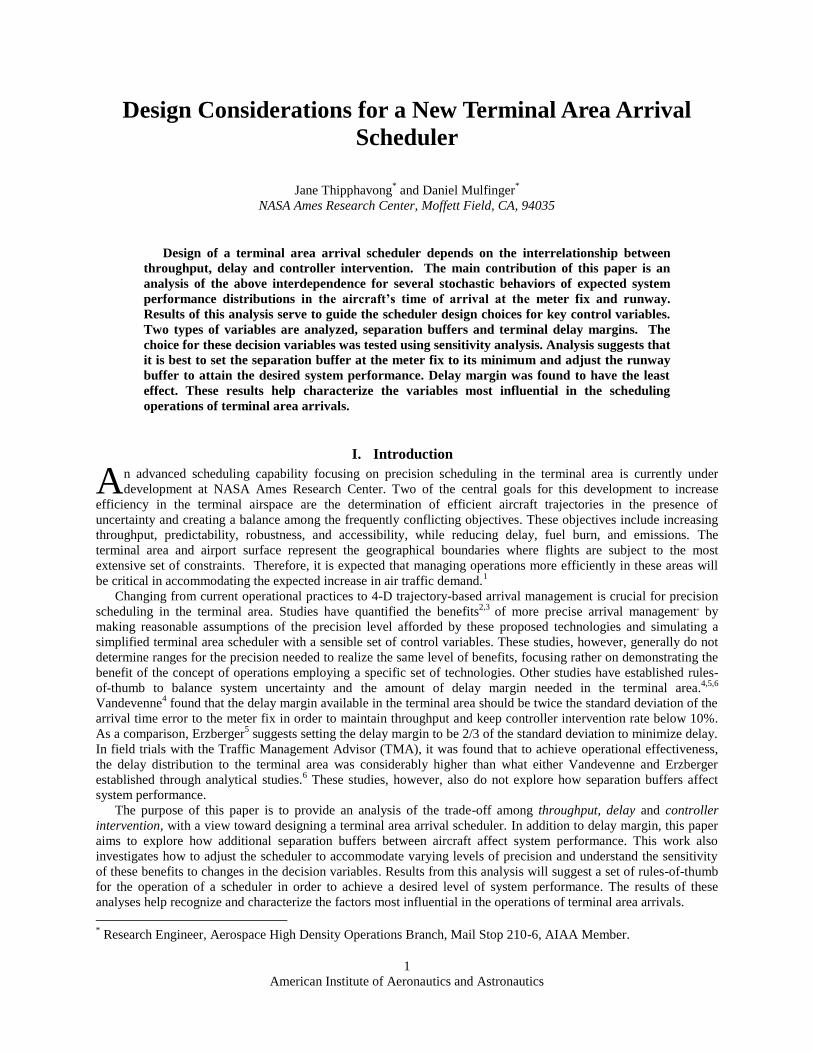
STASS7 was used in this study to simulate

aircraft sequencing and scheduling in both the

Air Route Traffic Control Center (Center) and

Terminal Radar Approach Control (TRACON)

airspace. Figure 1 shows the airspace topology

modeled in STASS, which includes two

scheduling points in the TRACON, the meter

fix and runway. Arrival times to the meter fixes

and runways, ATAmf and ATArwy are generated

by the Center Scheduler and the TRACON

Scheduler modules in STASS respectively. Any

number of meter fixes and runways can be

modeled. These basic scheduling locations are

typically used in terminal area scheduling

capabilities. The number of meter fixes and

runways chosen is dependent on the airport.

Analysis using STASS is intended to help

understand how scheduling metrics change Figure 1. STASS airspace topology.


3

when varying the control variables. These results then provide a starting point to choose the initial settings for the

terminal area scheduler being developed at NASA Ames Research Center. A basic overview of the scheduling

process is described next. Detailed description of the algorithm can be found in ref. 8.

Arrival aircraft originate from the Center boundary heading towards the meter fix. The Center Scheduler

determines the flight sequence as dictated by a first-come, first-served heuristic based on their unimpeded estimated

time of arrival, ETAmf. The scheduled arrival times, STAmf to the meter fixes are based on ETAmf, delay margin,

shortest time-to-fly (TTF) from the meter fix to runway, buffer b and separation requirement r for both the meter fix

and runway. The resulting meter fix arrival time STAmf computed by the Center Scheduler are proposed arrival times

that indicate when aircraft should arrive at the meter fixes. In cases where arrival times may not be met with

absolute delivery accuracy, these times are offset by an arrival time error, E. The actual time of arrival to the meter

fix is then calculated as ATAmf = STAmf + Emf.

The ATAmf + TTF is then used as ETArwy and as input into the TRACON Scheduler. The TRACON Scheduler

calculates STArwy by choosing the shortest TTF from the meter fix to runway and having r + b separation from the

leading aircraft. There may be an arrival time error in meeting the STArwy and so the ATArwy = STAmf + Erwy.

B. Simulation parameters

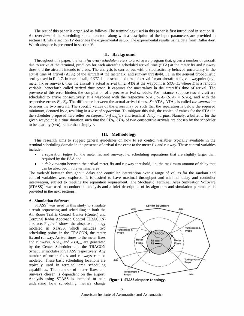
STASS includes the capability to model the stochastic behavior of the arrival time errors that occur in the

aircraft’s STAs to the meter fix and the runway threshold. This behavior can lead to either separation loss or to

unnecessary spacing between aircraft. The former effect compromises the safety of the terminal operation, while the

latter causes a waste of resources. STASS uses buffers and a delay margin in the terminal area to reduce the risk of

separation loss and

waste, respectively. It is

also recognized that

operationally, controllers

will not allow separation

to be compromised.

Thus, this is an indicator

to know when controller

intervention would be

required. To analyze the

interaction between the

control variables and the

stochastic arrival time

errors, a range of values

was chosen for each

variable such that it

spanned the most

realistic settings. Figure

2 is a stylized illustration

of when and where each

parameter is used in the

simulation.

IV. Experiment Setup

A. Dataset

The aircraft dataset was derived from Dallas/Fort Worth (DFW) TRACON traffic. NASA has used DFW as an

operational environment to study and test the applicability of its ATM technologies for many years. NASA has

gained a significant understanding of DFW operations through its access to vast amount of current air traffic data

and analyses.9,10

Based on this experience base, DFW was chosen for an initial assessment of the system behavior

using STASS.

The dataset had a throughput of approximately 168 aircraft per hour, which is considerably higher than today’s

operations (i.e. 126 aircraft per hour in visual meteorological conditions (VMC)).11

The number of aircraft in the

dataset was increased until the TRACON was fully saturated in STASS so that the analysis could be done on a high

demand scenario. DFW operates with two major configurations, North and South flow with aircraft landing and

Figure 2. Simulation parameters: 1) meter fix and runway arrival time uncertainty,

2) meter fix and runway buffer and 3) delay margin.


4

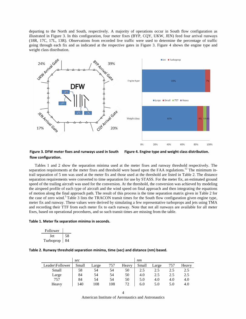
departing to the North and South, respectively. A majority of operations occur in South flow configuration as

illustrated in Figure 3. In this configuration, four meter fixes (BYP, CQY, UKW, JEN) feed four arrival runways

(18R, 17C, 17L, 13R). Observations from recorded live traffic were used to determine the percentage of traffic

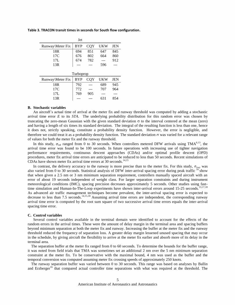
going through each fix and as indicated at the respective gates in Figure 3. Figure 4 shows the engine type and

weight class distribution.

Tables 1 and 2 show the separation minima used at the meter fixes and runway threshold respectively. The

separation requirements at the meter fixes and threshold were based upon the FAA regulations.12

The minimum in-

trail separation of 5 nm was used at the meter fix and those used at the threshold are listed in Table 2. The distance

separation requirements were converted to time separation for use by STASS. For the meter fix, an estimated ground

speed of the trailing aircraft was used for the conversion. At the threshold, the conversion was achieved by modeling

the airspeed profile of each type of aircraft and the wind speed on final approach and then integrating the equations

of motion along the final approach path. The result of this process is the time separation matrix given in Table 2 for

the case of zero wind.5

Table 3 lists the TRACON transit times for the South flow configuration given engine type,

meter fix and runway. These values were derived by simulating a few representative turboprops and jets using TMA

and recording their TTF from each meter fix to each runway. Note that not all runways are available for all meter

fixes, based on operational procedures, and so such transit times are missing from the table.

Table 1. Meter fix separation minima in seconds.

Follower

Jet 58

Turboprop 84

Table 2. Runway threshold separation minima, time (sec) and distance (nm) based.

sec nm

Leader\Follower Small Large 757 Heavy Small Large 757 Heavy

Small 58 54 54 50 2.5 2.5 2.5 2.5

Large 84 54 54 50 4.0 2.5 2.5 2.5

757 84 54 54 50 5.0 4.0 4.0 4.0

Heavy 140 108 108 72 6.0 5.0 5.0 4.0

Figure 3. DFW meter fixes and runways used in South

flow configuration.

Figure 4. Engine type and weight class distribution.


5

Table 3. TRACON transit times in seconds for South flow configuration.

Jet

Runway\Meter Fix BYP CQY UKW JEN

18R 694 851 647 845

17C 676 802 664 860

17L 674 782 --- 912

13R --- --- 596 ---

Turboprop

Runway\Meter Fix BYP CQY UKW JEN

18R 792 --- 689 945

17C 772 --- 707 964

17L 769 905 --- ---

13R --- --- 631 854

B. Stochastic variables

An aircraft’s actual time of arrival at the meter fix and runway threshold was computed by adding a stochastic

arrival time error E to its STA. The underlying probability distribution for this random error was chosen by

truncating the zero-mean Gaussian with the given standard deviation to the interval centered at the mean (zero)

and having a length of six times its standard deviation. The integral of the resulting function is less than one, hence

it does not, strictly speaking, constitute a probability density function. However, the error is negligible, and

therefore we could treat it as a probability density function. The standard deviation was varied for a relevant range

of values for both the meter fix and the runway threshold.

In this study, mf ranged from 0 to 30 seconds. When controllers metered DFW arrivals using TMA6,13

, the

arrival time error was found to be 100 seconds. In future operations with increasing use of tighter navigation

performance requirements, continuous descent approaches (CDAs) and/or optimal profile descent (OPD)

procedures, meter fix arrival time errors are anticipated to be reduced to less than 50 seconds. Recent simulations of

CDAs have shown meter fix arrival time errors at 30 seconds.14,15

In contrast, the delivery accuracy to the runway is more precise than to the meter fix. For this study, rwy was

also varied from 0 to 30 seconds. Statistical analysis of DFW inter-arrival spacing error during peak traffic 16

show

that when given a 2.5 nm or 3 nm minimum separation requirement, controllers manually spaced aircraft with an

error of about 19 seconds independent of weight class. For larger separation constraints and during instrument

meteorological conditions (IMC), spacing precision decreases approximately 5 seconds. Other studies using fast-

time simulation and Human-In-The-Loop experiments have shown inter-arrival errors around 15-25 seconds.13,17,18

As advanced air traffic management techniques become prevalent, the inter-arrival spacing error is expected to

decrease to less than 7.5 seconds.14,15,18

Assuming arrival time errors are independent, the corresponding runway

arrival time error is computed by the root sum square of two successive arrival time errors equals the inter-arrival

spacing time error.

C. Control variables

Several control variables available in the terminal domain were identified to account for the effects of the

random errors in the arrival times. These were the amount of delay margin in the terminal area and spacing buffers

beyond minimum separation at both the meter fix and runway. Increasing the buffer at the meter fix and the runway

threshold reduced the frequency of separation loss. A greater delay margin lessened unused spacing that may occur

in the schedule, by giving aircraft the flexibility to arrive at the meter fix earlier and absorb more of its delay in the

terminal area.

The separation buffer at the meter fix ranged from 0 to 60 seconds. To determine the bounds for the buffer range,

it was noted from field trials that TMA was sometimes set an additional 2 nm over the 5 nm minimum separation

constraint at the meter fix. To be conservative with the maximal bound, 4 nm was used as the buffer and the

temporal conversion was computed assuming meter fix crossing speeds of approximately 250 knots.

The runway separation buffer was varied between 0 to 30 seconds. This range was based on analyses by Ballin

and Erzberger16

that compared actual controller time separations with what was required at the threshold. The


6

difference between these two values was used as the runway buffer and varied between 5 to 30 seconds between

different weight class pairs, separation requirements and meteorological conditions.

The delay margin ranged from 5% to 25% of an aircraft’s TTF from the meter fix to the runway. As RNAV

approaches and CDAs are encouraged in future operating concepts, the controllability within the terminal area will

be restricted in order to maintain an efficient schedule and maximize the benefits of such procedures. A prior study

estimated that an aircraft can absorb delay of about 10% its TTF by using only speed control.14

Table 4. Summary of stochastic and control variables and range of values studied.

Stochastic variables Min Max Control variables Min Max

mf 0s 30s Meter fix buffer 0s 60s

rwy 0s 30s Runway buffer 0s 30s

Delay margin 5%TTF 25%TTF

V. Results

A series of simulations were conducted to study how airport throughput, delay and the number of controller

interventions were affected by the range of control and random variables typically present in the terminal area

domain. The tradeoffs between throughput, delay, and controller intervention were then examined to gain insight on

how to best set the control variables available in a terminal area scheduler. These variables include 1) the buffer at

the arrival metering fix, 2) the buffer at the runway threshold and 3) the delay margin between the arrival metering

fix and runway threshold. Given a set of values for each stochastic and control variable, 500 Monte Carlo

simulations were run. For each Monte Carlo simulation, each aircraft was given a stochastic arrival time at both the

meter fix and runway based on arrival time error term E chosen from the truncated Gaussian distribution with mean

at zero and the chosen σ value. The metrics shown in the results section are an average over all 500 runs.

Definitions for the metrics used to study the tradeoffs are given below.

Airport throughput is used as an indicator on how well the scheduler performs. With the anticipated increase in

air traffic demand, methods to increase or at least maintain throughput are of particular interest for the future air

traffic management system. There are several ways to measure throughput. In this study throughput is defined as

follows:

Delay an aircraft consumes in order to meet its scheduled time of arrival is calculated as the difference between

its estimated time of arrival and actual time of arrival. This quantity is defined for both the runway and meter fix,

denoted by the subscript rwy and mf respectively:

Controller intervention during air traffic management may be exercised for a number of reasons which include

keeping traffic safely separated, meeting a scheduled time of arrival at a point, heeding traffic flow management

restrictions or responding to a pilot’s request. For this study, the number of aircraft that stochastically incur a loss of

separation due to arrival time error is counted as necessitated intervention by a controller. Controller intervention is

the probability of a loss of separation, i.e. of the event X<r.

A. Stochastic variables

The general effect of how uncertainty in arrival times affects simulation results is detailed in this section. For

these simulation runs, an offset value was added to the scheduled time of arrival of each aircraft (which is its ATA)

to simulate the imperfect delivery accuracy when meeting a given arrival time at both the runway and meter fix. The

offset value was chosen from a truncated nearly Gaussian distribution centered at zero seconds and having a

maximum/minimum spread of ±3σ.


7

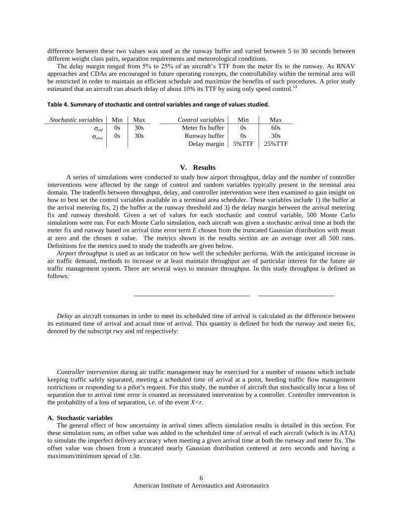
1. Throughput

Figure 5 shows the relationship between

the average runway throughput and arrival

time error for both the meter fix and runway

when the delay margin is set to 10% of an

aircraft’s time-to-fly (TTF) and the meter fix

and runway buffers are set to 0. There is a

minimal decline in throughput as σmf

increases from 0 to 30 seconds and virtually

no change when increasing σrwy in the same

range. For other scenarios with non zero

runway and/or meter fix buffer values, delay

margin changes, the change in average

runway throughput when varying the

uncertainty, are still minimal (i.e. less than

one aircraft per hour).

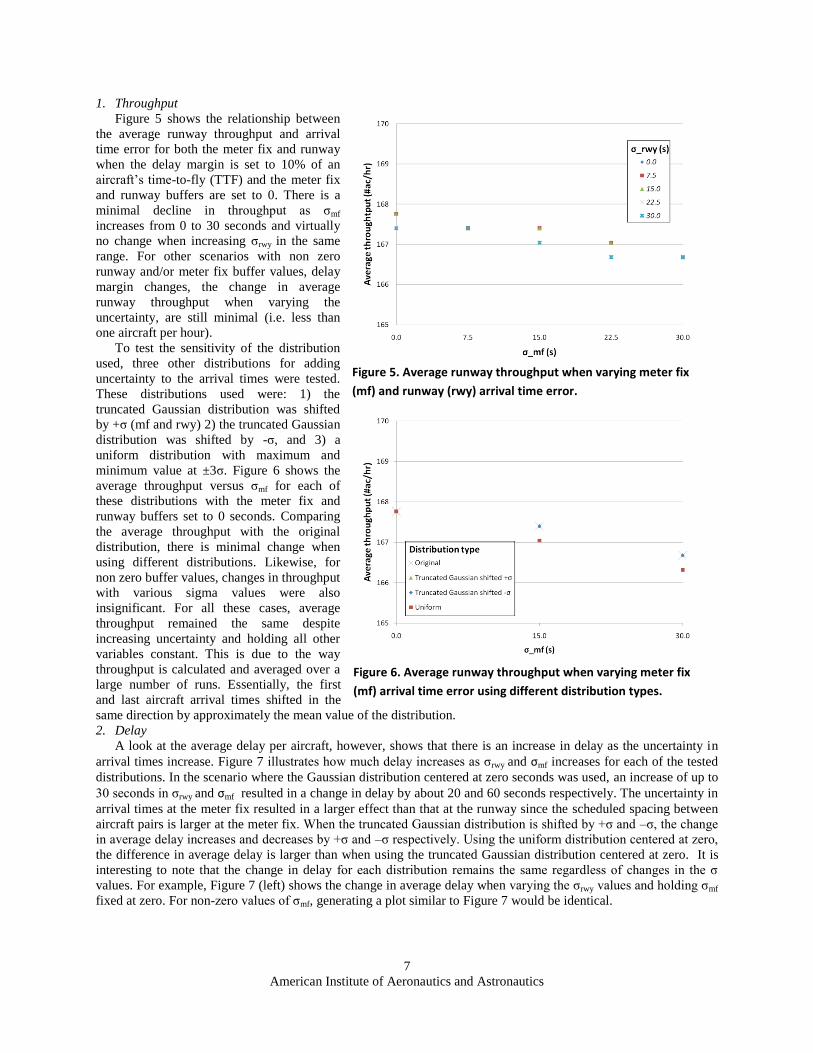
To test the sensitivity of the distribution

used, three other distributions for adding

uncertainty to the arrival times were tested.

These distributions used were: 1) the

truncated Gaussian distribution was shifted

by +σ (mf and rwy) 2) the truncated Gaussian

distribution was shifted by -σ, and 3) a

uniform distribution with maximum and

minimum value at ±3σ. Figure 6 shows the

average throughput versus σmf for each of

these distributions with the meter fix and

runway buffers set to 0 seconds. Comparing

the average throughput with the original

distribution, there is minimal change when

using different distributions. Likewise, for

non zero buffer values, changes in throughput

with various sigma values were also

insignificant. For all these cases, average

throughput remained the same despite

increasing uncertainty and holding all other

variables constant. This is due to the way

throughput is calculated and averaged over a

large number of runs. Essentially, the first

and last aircraft arrival times shifted in the

same direction by approximately the mean value of the distribution.

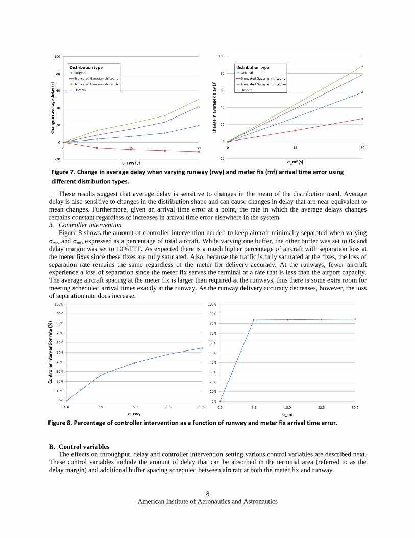
2. Delay

A look at the average delay per aircraft, however, shows that there is an increase in delay as the uncertainty in

arrival times increase. Figure 7 illustrates how much delay increases as σrwy and σmf increases for each of the tested

distributions. In the scenario where the Gaussian distribution centered at zero seconds was used, an increase of up to

30 seconds in σrwy and σmf resulted in a change in delay by about 20 and 60 seconds respectively. The uncertainty in

arrival times at the meter fix resulted in a larger effect than that at the runway since the scheduled spacing between

aircraft pairs is larger at the meter fix. When the truncated Gaussian distribution is shifted by +σ and –σ, the change

in average delay increases and decreases by +σ and –σ respectively. Using the uniform distribution centered at zero,

the difference in average delay is larger than when using the truncated Gaussian distribution centered at zero. It is

interesting to note that the change in delay for each distribution remains the same regardless of changes in the σ

values. For example, Figure 7 (left) shows the change in average delay when varying the σrwy values and holding σmf

fixed at zero. For non-zero values of σmf, generating a plot similar to Figure 7 would be identical.

Figure 5. Average runway throughput when varying meter fix

(mf) and runway (rwy) arrival time error.

Figure 6. Average runway throughput when varying meter fix

(mf) arrival time error using different distribution types.


8

These results suggest that average delay is sensitive to changes in the mean of the distribution used. Average

delay is also sensitive to changes in the distribution shape and can cause changes in delay that are near equivalent to

mean changes. Furthermore, given an arrival time error at a point, the rate in which the average delays changes

remains constant regardless of increases in arrival time error elsewhere in the system.

3. Controller intervention

Figure 8 shows the amount of controller intervention needed to keep aircraft minimally separated when varying

σrwy and σmf, expressed as a percentage of total aircraft. While varying one buffer, the other buffer was set to 0s and

delay margin was set to 10%TTF. As expected there is a much higher percentage of aircraft with separation loss at

the meter fixes since these fixes are fully saturated. Also, because the traffic is fully saturated at the fixes, the loss of

separation rate remains the same regardless of the meter fix delivery accuracy. At the runways, fewer aircraft

experience a loss of separation since the meter fix serves the terminal at a rate that is less than the airport capacity.

The average aircraft spacing at the meter fix is larger than required at the runways, thus there is some extra room for

meeting scheduled arrival times exactly at the runway. As the runway delivery accuracy decreases, however, the loss

of separation rate does increase.

B. Control variables

The effects on throughput, delay and controller intervention setting various control variables are described next.

These control variables include the amount of delay that can be absorbed in the terminal area (referred to as the

delay margin) and additional buffer spacing scheduled between aircraft at both the meter fix and runway.

Figure 7. Change in average delay when varying runway (rwy) and meter fix (mf) arrival time error using

different distribution types.

Figure 8. Percentage of controller intervention as a function of runway and meter fix arrival time error.


9

1. Throughput

The FAA has developed guidelines specifying minimum separation requirements for all combinations of

leading and following aircraft type as specified in Tables 1 and 2. Exact spacing between aircraft cannot always be

achieved. Setting the spacing beyond the minimum spacing requirements provides a buffer for the controllers to

handle uncertainties in the system. During busy traffic periods, however, this added separation between aircraft

results in a reduction in throughput.

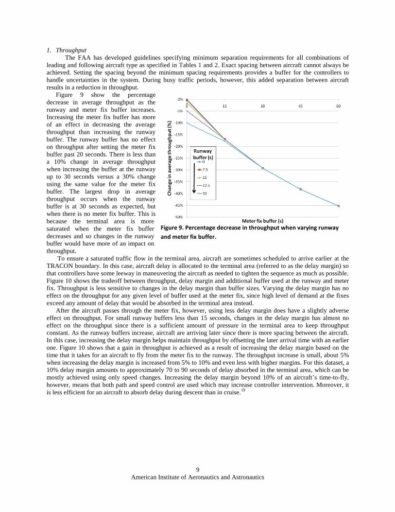
Figure 9 show the percentage

decrease in average throughput as the

runway and meter fix buffer increases.

Increasing the meter fix buffer has more

of an effect in decreasing the average

throughput than increasing the runway

buffer. The runway buffer has no effect

on throughput after setting the meter fix

buffer past 20 seconds. There is less than

a 10% change in average throughput

when increasing the buffer at the runway

up to 30 seconds versus a 30% change

using the same value for the meter fix

buffer. The largest drop in average

throughput occurs when the runway

buffer is at 30 seconds as expected, but

when there is no meter fix buffer. This is

because the terminal area is more

saturated when the meter fix buffer

decreases and so changes in the runway

buffer would have more of an impact on

throughput.

To ensure a saturated traffic flow in the terminal area, aircraft are sometimes scheduled to arrive earlier at the

TRACON boundary. In this case, aircraft delay is allocated to the terminal area (referred to as the delay margin) so

that controllers have some leeway in maneuvering the aircraft as needed to tighten the sequence as much as possible.

Figure 10 shows the tradeoff between throughput, delay margin and additional buffer used at the runway and meter

fix. Throughput is less sensitive to changes in the delay margin than buffer sizes. Varying the delay margin has no

effect on the throughput for any given level of buffer used at the meter fix, since high level of demand at the fixes

exceed any amount of delay that would be absorbed in the terminal area instead.

After the aircraft passes through the meter fix, however, using less delay margin does have a slightly adverse

effect on throughput. For small runway buffers less than 15 seconds, changes in the delay margin has almost no

effect on the throughput since there is a sufficient amount of pressure in the terminal area to keep throughput

constant. As the runway buffers increase, aircraft are arriving later since there is more spacing between the aircraft.

In this case, increasing the delay margin helps maintain throughput by offsetting the later arrival time with an earlier

one. Figure 10 shows that a gain in throughput is achieved as a result of increasing the delay margin based on the

time that it takes for an aircraft to fly from the meter fix to the runway. The throughput increase is small, about 5%

when increasing the delay margin is increased from 5% to 10% and even less with higher margins. For this dataset, a

10% delay margin amounts to approximately 70 to 90 seconds of delay absorbed in the terminal area, which can be

mostly achieved using only speed changes. Increasing the delay margin beyond 10% of an aircraft’s time-to-fly,

however, means that both path and speed control are used which may increase controller intervention. Moreover, it

is less efficient for an aircraft to absorb delay during descent than in cruise.19

Figure 9. Percentage decrease in throughput when varying runway

and meter fix buffer.


10

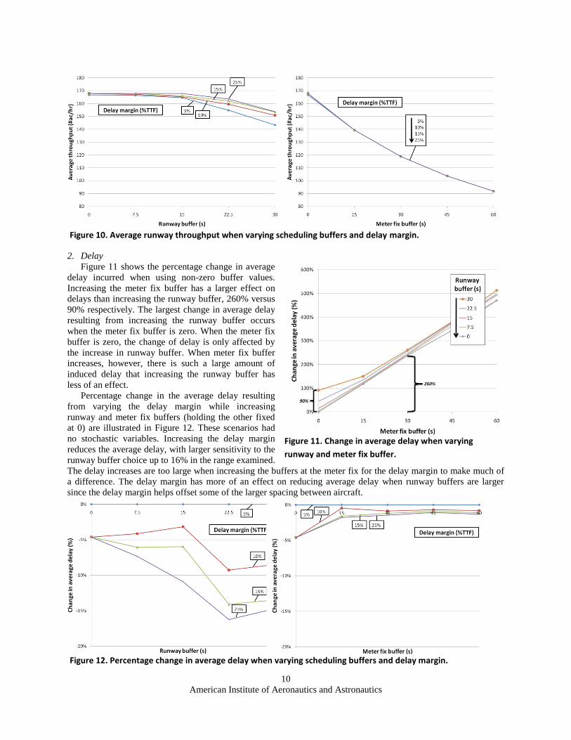
2. Delay

Figure 11 shows the percentage change in average

delay incurred when using non-zero buffer values.

Increasing the meter fix buffer has a larger effect on

delays than increasing the runway buffer, 260% versus

90% respectively. The largest change in average delay

resulting from increasing the runway buffer occurs

when the meter fix buffer is zero. When the meter fix

buffer is zero, the change of delay is only affected by

the increase in runway buffer. When meter fix buffer

increases, however, there is such a large amount of

induced delay that increasing the runway buffer has

less of an effect.

Percentage change in the average delay resulting

from varying the delay margin while increasing

runway and meter fix buffers (holding the other fixed

at 0) are illustrated in Figure 12. These scenarios had

no stochastic variables. Increasing the delay margin

reduces the average delay, with larger sensitivity to the

runway buffer choice up to 16% in the range examined.

The delay increases are too large when increasing the buffers at the meter fix for the delay margin to make much of

a difference. The delay margin has more of an effect on reducing average delay when runway buffers are larger

since the delay margin helps offset some of the larger spacing between aircraft.

Figure 10. Average runway throughput when varying scheduling buffers and delay margin.

Figure 11. Change in average delay when varying

runway and meter fix buffer.

Figure 12. Percentage change in average delay when varying scheduling buffers and delay margin.


11

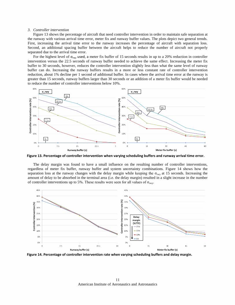
3. Controller intervention

Figure 13 shows the percentage of aircraft that need controller intervention in order to maintain safe separation at

the runway with various arrival time error, meter fix and runway buffer values. The plots depict two general trends.

First, increasing the arrival time error to the runway increases the percentage of aircraft with separation loss.

Second, an additional spacing buffer between the aircraft helps to reduce the number of aircraft not properly

separated due to the arrival time error.

For the highest level of σrwy used, a meter fix buffer of 15 seconds results in up to a 20% reduction in controller

intervention versus the 22.5 seconds of runway buffer needed to achieve the same effect. Increasing the meter fix

buffer to 30 seconds, however, reduces the controller intervention slightly less than what the same level of runway

buffer can do. Increasing the runway buffers results in a more or less constant rate of controller intervention

reduction, about 1% decline per 1 second of additional buffer. In cases where the arrival time error at the runway is

greater than 15 seconds, runway buffers larger than 30 seconds or an addition of a meter fix buffer would be needed

to reduce the number of controller interventions below 10%.

The delay margin was found to have a small influence on the resulting number of controller interventions,

regardless of meter fix buffer, runway buffer and system uncertainty combinations. Figure 14 shows how the

separation loss at the runway changes with the delay margin while keeping the σrwy at 15 seconds. Increasing the

amount of delay to be absorbed in the terminal area (i.e. the delay margin) resulted in a slight increase in the number

of controller interventions up to 5%. These results were seen for all values of σrwy.

Figure 13. Percentage of controller intervention when varying scheduling buffers and runway arrival time error.

Figure 14. Percentage of controller intervention rate when varying scheduling buffers and delay margin.


12

C. Scheduler design considerations

One use of these results is to help understand how scheduler parameters should be set for a desired operational

concept. For example, NASA Ames Research Center is testing a mid-term concept for super-dense terminal area

operations that investigates the effect of utilizing more precise scheduling. The scheduler used in this concept is

based on the TMA,20

where aircraft are scheduled to both the meter fix and runway adhering to minimum separation

requirements and arrival rate constraints. These aircraft are assigned a fixed route approximately 200 nm prior to

entering the terminal area boundary. Controllers are then expected to meet meter fix and runway arrival times

produced by the scheduler within 30 and 15 seconds respectively, while using speed adjustments as the primary

means of control in the terminal area.

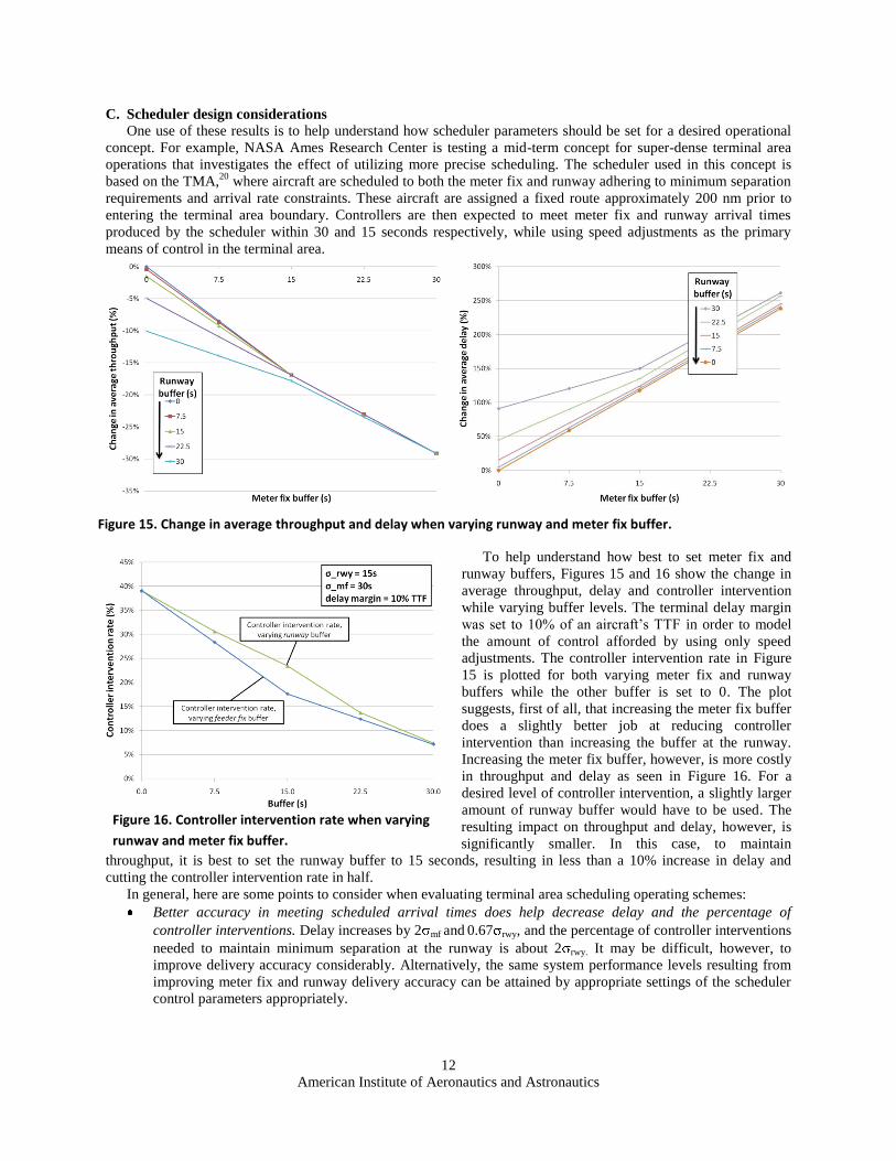
To help understand how best to set meter fix and

runway buffers, Figures 15 and 16 show the change in

average throughput, delay and controller intervention

while varying buffer levels. The terminal delay margin

was set to 10% of an aircraft’s TTF in order to model

the amount of control afforded by using only speed

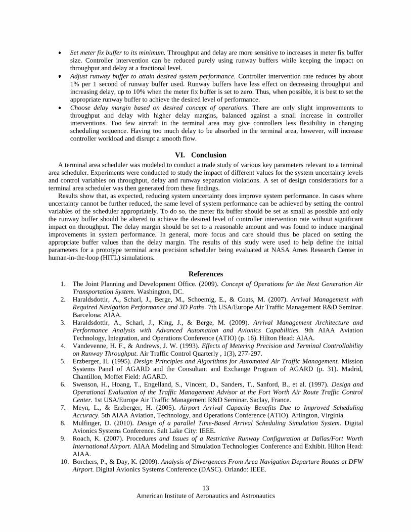
adjustments. The controller intervention rate in Figure

15 is plotted for both varying meter fix and runway

buffers while the other buffer is set to 0. The plot

suggests, first of all, that increasing the meter fix buffer

does a slightly better job at reducing controller

intervention than increasing the buffer at the runway.

Increasing the meter fix buffer, however, is more costly

in throughput and delay as seen in Figure 16. For a

desired level of controller intervention, a slightly larger

amount of runway buffer would have to be used. The

resulting impact on throughput and delay, however, is

significantly smaller. In this case, to maintain

throughput, it is best to set the runway buffer to 15 seconds, resulting in less than a 10% increase in delay and

cutting the controller intervention rate in half.

In general, here are some points to consider when evaluating terminal area scheduling operating schemes:

Better accuracy in meeting scheduled arrival times does help decrease delay and the percentage of

controller interventions. Delay increases by 2 mf and 0.67 rwy, and the percentage of controller interventions

needed to maintain minimum separation at the runway is about 2 rwy. It may be difficult, however, to

improve delivery accuracy considerably. Alternatively, the same system performance levels resulting from

improving meter fix and runway delivery accuracy can be attained by appropriate settings of the scheduler

control parameters appropriately.

Figure 15. Change in average throughput and delay when varying runway and meter fix buffer.

Figure 16. Controller intervention rate when varying

runway and meter fix buffer.


13

Set meter fix buffer to its minimum. Throughput and delay are more sensitive to increases in meter fix buffer

size. Controller intervention can be reduced purely using runway buffers while keeping the impact on

throughput and delay at a fractional level.

Adjust runway buffer to attain desired system performance. Controller intervention rate reduces by about

1% per 1 second of runway buffer used. Runway buffers have less effect on decreasing throughput and

increasing delay, up to 10% when the meter fix buffer is set to zero. Thus, when possible, it is best to set the

appropriate runway buffer to achieve the desired level of performance.

Choose delay margin based on desired concept of operations. There are only slight improvements to

throughput and delay with higher delay margins, balanced against a small increase in controller

interventions. Too few aircraft in the terminal area may give controllers less flexibility in changing

scheduling sequence. Having too much delay to be absorbed in the terminal area, however, will increase

controller workload and disrupt a smooth flow.

VI. Conclusion

A terminal area scheduler was modeled to conduct a trade study of various key parameters relevant to a terminal

area scheduler. Experiments were conducted to study the impact of different values for the system uncertainty levels

and control variables on throughput, delay and runway separation violations. A set of design considerations for a

terminal area scheduler was then generated from these findings.

Results show that, as expected, reducing system uncertainty does improve system performance. In cases where

uncertainty cannot be further reduced, the same level of system performance can be achieved by setting the control

variables of the scheduler appropriately. To do so, the meter fix buffer should be set as small as possible and only

the runway buffer should be altered to achieve the desired level of controller intervention rate without significant

impact on throughput. The delay margin should be set to a reasonable amount and was found to induce marginal

improvements in system performance. In general, more focus and care should thus be placed on setting the

appropriate buffer values than the delay margin. The results of this study were used to help define the initial

parameters for a prototype terminal area precision scheduler being evaluated at NASA Ames Research Center in

human-in-the-loop (HITL) simulations.

References

1. The Joint Planning and Development Office. (2009). Concept of Operations for the Next Generation Air

Transportation System. Washington, DC.

2. Haraldsdottir, A., Scharl, J., Berge, M., Schoemig, E., & Coats, M. (2007). Arrival Management with

Required Navigation Performance and 3D Paths. 7th USA/Europe Air Traffic Management R&D Seminar.

Barcelona: AIAA.

3. Haraldsdottir, A., Scharl, J., King, J., & Berge, M. (2009). Arrival Management Architecture and

Performance Analysis with Advanced Automation and Avionics Capabilities. 9th AIAA Aviation

Technology, Integration, and Operations Conference (ATIO) (p. 16). Hilton Head: AIAA.

4. Vandevenne, H. F., & Andrews, J. W. (1993). Effects of Metering Precision and Terminal Controllability

on Runway Throughput. Air Traffic Control Quarterly , 1(3), 277-297.

5. Erzberger, H. (1995). Design Principles and Algorithms for Automated Air Traffic Management. Mission

Systems Panel of AGARD and the Consultant and Exchange Program of AGARD (p. 31). Madrid,

Chantillon, Moffet Field: AGARD.

6. Swenson, H., Hoang, T., Engelland, S., Vincent, D., Sanders, T., Sanford, B., et al. (1997). Design and

Operational Evaluation of the Traffic Management Advisor at the Fort Worth Air Route Traffic Control

Center. 1st USA/Europe Air Traffic Management R&D Seminar. Saclay, France.

7. Meyn, L., & Erzberger, H. (2005). Airport Arrival Capacity Benefits Due to Improved Scheduling

Accuracy. 5th AIAA Aviation, Technology, and Operations Conference (ATIO). Arlington, Virginia.

8. Mulfinger, D. (2010). Design of a parallel Time-Based Arrival Scheduling Simulation System. Digital

Avionics Systems Conference. Salt Lake City: IEEE.

9. Roach, K. (2007). Procedures and Issues of a Restrictive Runway Configuration at Dallas/Fort Worth

International Airport. AIAA Modeling and Simulation Technologies Conference and Exhibit. Hilton Head:

AIAA.

10. Borchers, P., & Day, K. (2009). Analysis of Divergences From Area Navigation Departure Routes at DFW

Airport. Digital Avionics Systems Conference (DASC). Orlando: IEEE.


14

11. FAA. (2010, August 18). ATCSCC OIS System. Retrieved August 18, 2010, from

http://www.fly.faa.gov/ois/

12. FAA. (2010, February 11). U.S. Department of Transportation Federal Aviation Administration Air.

Retrieved August 18, 2010, from Air Traffic Organization Policy Order JO 7110.65T:

http://www.faa.gov/air_traffic/publications/atpubs/atc/

13. Denery, D. G., & Erzberger, H. (1995). The Center-TRACON Automation System: Simulation and Field

Testing. Moffett Field, CA: NASA Ames Research Center.

14. Barmore, B. E., Abbott, T. S., Capron, W. R., & Baxley, B. T. (2008). Simulation Results for Airborne

Precision Spacing along Continuous Descent Arrivals. AIAA Aviation Technology, Integration and

Operations Conference. Anchorage, AK.

15. Murdoch, J. L., Barmore, B. E., Abbott, T. S., & Capron, W. R. (2009). Evaluation of an Airborne Spacing

Concept to Support Continuous Descent Arrival Operations. Eigth USA/Europe Air Traffic Management

Research and Development Seminar. Napa, California.

16. Ballin, M., & Erzberger, H. (1996). An Analysis of Landing Rates and Separations at the Dallas/Fort

Worth International Airport. NASA Technical Memorandum 110397.

17. Credeur, L., Capron, W. R., Lohr, G. W., Crawford, D. J., Tang, D. A., & Rodgers, W. G. (1993). Final-

Approach Spacing Aids (FASA) Evaluation For Terminal-Area, Time-Based Air Traffic Control. Moffett

Field, CA: NASA Ames Research Center.

18. Boursier, L., Favennec, B., Hoffman, E., Trzmiel, A., Vergne, F., & Zeghal, K. (2007). Merging Arrival

Flows Without Heading Instructions. 7th USA/Europe Air Traffic Mangement R&D Seminar. Barcelona,

Spain.

19. Robinson, J. (2010). Benefits of Continuous Descent Operations in High-Density Terminal Airspace Under

Scheduling Constraints. Aviation Technology, Integration, And Operations (ATIO) Conference. AIAA.

20. Wong, G. (2000). The Dynamic Planner: The Sequencer, Scheduler, and Runway Allocator for Air Traffic

Control Automation. Moffet Field: NASA .

Documents

Design Considerations for a New Terminal Area Arrival