Embed Size (px)
DESCRIPTION
research and design of the buildings assisted by testings.
Citation preview

DESIGN ASSISTED BY TESTING
Part I
Prof. Raul ZAHARIA

1 . Basics
1.1 Why to perform an experimental test
Daily, we have information about the evolution of different variables, for which high precision
is not required, such as the indoor/ outside temperature (for which an accuracy of one degree
Celsius may be enough). On the other hand, when it is necessary to determine the body
temperature, more precise measurements are needed. In such cases, the selection of equipment,
measurement techniques and interpretation of measured data should require more attention.
The purpose of an experimental test is to determine the value or the trend of evolution of a
variable.
Another definition: the test at which is subjected a "product", in order to prove that it meets the
expected characteristics/ performance.
In fact, there are different types of experimental tests that are better suited to one or other of
the definitions.
1.2 Types of experimental tests
Experimental tests may be of different types: research, examination (certification), or control
(quality control). This classification follows somehow the chronological order to develop a
product: design, manufacture, and marketing. Research tests implies the study of a product:
• reduced model tests ( example in Figure 1.1) ;
• tests on details ( examples in Figures 1.2-3 );
• tests on substructures ( example in Figure 1.4);
tests at real scale ( example in Figure 1.5)
• laboratory test
• testing in situ
• destructive tests
• non destructive testing

Fig. 1.1 Reduced scale model of Sport Hall roof in Craiova - CMMC Department
Fig. 1.2 Test on joint Sport Hall roof in Craiova - CMMC Department

Fig. 1.3 Test on typical joint for cold-formed steel trusses with bolted connections
- CMMC Department

Fig. 1.4 Test on a truss substructure – CMMC Department

Fig. 1.5 Full scale test in pseudo-dynamic regime - ELSA laboratory of the
European Commission in Ispra, Italy

Certification experimental tests demonstrate the compliance of a product with technical
specifications or standards.
This type of tests, particularly demanding, are usually standardized, and are performed in
certified laboratories.
Example: fire resistance of a wall panel – mechanical resistance/ integrity/ insulation – in
specialized laboratories (Figure 1.6 – furnace).
Fig. 1.6 Furnace for determining the fire resistance of vertical elements
Quality control experimental tests should confirm the characteristics of a product and are
usually performed before commercialization.
This type of experimental investigation involves regular testing of one or more elements of a
production series. For example, on-site delivery of steel profiles, come accompanied by the
mechanical characteristics (example S235J0/J2...).

1.3 . Experimental test set-up
Infrastructure:
• building test laboratory :
- conception (including foundation);
- access ;
- lifting devices;
- storage areas ;
- equipment.
Loading devices :
• universal testing machine ;
• reaction frames;
• actuators.
Measuring devices - transducers:
• displacements (mechanical / electrical ) ;
• strain (strain gauges, 3D video, etc.);
• forces ( mechanical / electrical ).
1.4 Components of a measuring system
The measurement can be defined as the act of assigning a value to a physical variable.
A measurement system is therefore a tool for quantifying physical variables.
A variable may be:
• independent - if varies independently of any other variables;
• dependent - if it is affected by changes in one or more of other variables.

For instance, in determining the boiling temperature of water, if the measurement is performed
in open environmental conditions in three different days, three different results may be obtained
(conditions for measurement are identical, excepting for the atmospheric pressure that may be
different from one day to another).
The control of the variables is important. A variable is said to be controlled if it can be kept at
a constant value during the measurement. A perfect control is not always possible and therefore
the term "control” is used to refer to a variable that can be fixed in nominal sense.
Variables may have:
• discrete values (eg: values obtained while throwing a dice);
• continue values (eg: displacement , pressure, etc).
The variables that cannot be controlled during the measurement, but affect the measure of other
variables. are called external variables. They produce overlapping signals within the measured
signal, creating noise and interference.
Noise is a random variation of the measured signal value as a consequence of the variation of
the external variables (eg: electric random fluctuation) .
Interference produce unwanted jumps in the measured signal, as a consequence of the variation
of the external variables (eg interference from motors, welding equipment).
The parameter is defined as a relationship between variables.
A parameter that has an effect on the behavior of the measured variables is called “control
parameter”. A parameter considered to be controlled, is a parameter considered as constant
during a test.

Components of the measuring system:
• Sensor
• Transducer
• Signal conditioning (optional)
• Output
• Control (optional)
The sensor is the physical element that uses a natural phenomenon that feels the variable to be
measured (eg the classic thermometer - mercury fluid volume that changes with temperature
variation).
The transducer converts the information into a signal (which can be mechanical, electrical,
optical, etc.). The goal is to convert the information into a form that can be easily quantified
(eg classic mercury thermometer - the bulb acts as a transducer - information exchange: thermal
expansion information by forcing fluid mechanics in a capillary).
Output (exit) gives an indication of the value of measurement. The output may be a simple
display (eg for the classic mercury thermometer - graduated scale).
Signal Conditioning (Optional) may be used to increase the signal magnitude by amplification,
by removing portions of the signal filtering techniques, etc. (eg the classic thermometer
mercury: capillarity diameter determines how fluid moves when temperature changes: smaller
the diameter = bigger the displacement = better the precision of the measurement).
Control (feedback) implies the existence of a controller that interprets the measured signal and
decides on process control (eg for motors, at a certain temperature, there are security systems
that can be activated to avoid overheating).
The relationship between the input information (input) and the output is determined by a
calibration. Calibration is the process of applying known input values (calibers) in order to
observe the output value. For instance, in order to build a classic mercury thermometer we may
apply known values of temperature in order to determine the correct grading scale).

2. Measurement Errors
The measurement error is represented by the difference between the measured output signal
and the exact value of the measure m. This last value being unknown, the measurement error
can only be estimated.
The precision of the output signal depends on the transducer, but also on the data aquisition
system at which the transducer is linked.
There are two types of errors:
- systematic errors;
- accidental errors.
The systematic errors are introducing a constant gap between the actual value of the physical
variable and the measured value. Systematic errors actually result from an improper use of data
acquisition devices and may be reduced by precise knowledge and rigorous use of these devices.
Systematic errors:
- errors due to the use of the transducers in environmental conditions (temperature, humidity...)
not complying with those provided in the producer specifications;
- errors in the transducer characteristics, as considering a wrong calibration; this type of error
can be reduced by performing a regular recalibration;
- errors due to the wrong utilisation of the transducer, eg not respecting the response time.
The accidental errors are random errors that may occur suddenly and indefinitely. The various
causes of accidental errors generators are related to:
- external variables and their variation during the measuremnent;
- improper positioning or change of the position of the transducer during the test;
- noise and interference
For a better understanding of the difference between the accidental and systematic errors , let’s
consider the example of a displacement transducer and two different modes of operation of the
test:
- in the first case, the transducer is fixed in position and the test is performed n times;
- in the second case, before each of the n measurements, the transducer is repositioned.

In the first case, the error introduced is systematic, while in the second case it becomes
accidental.
Statistical treatment of results aims to determine the most probable value of the measured
quantity. The statistical treatment of the results refers only to accidental errors, hence the
importance of the distinction between accidental and systematic errors made previously.
When measuring the same quantity m was repeated n times , the mean measurement is defined
as:
1 2 ... nm m mm
n
+ + +=
A measure of the dispersion of the measured values from the average value is given by the
standard deviation:
( ) ( ) ( )2 2 2
1 2 ...
1
nm m m m m m
nσ
− + − + + −=
−
Assuming that accidental errors are independent, it is accepted that the distribution of results
follows the Gauss probability curve. The probability P(m1, m2) to get me a measurement result
in the range of two values m1, m2 is given by:
2
1
( 1, 2) ( )
m
m
P m m p m dm= ∫
in which p(m) is the probability density value of the measure m (Gauss Law):
( )2
2
1( ) exp
22
m mp m
σσ π
− = −
The most probable value of the test value is the mean value.
The probability P (in %) of occurrence of an outcome within different ranges:
mean value + / - 1 standard deviation = 68.27%
mean value + / - 2 standard deviation = 95.45%
mean value + / - 3 standard deviation = 99.73%

Fig. 2.1 Gauss Law
The precision of a measurement device is given by both accuracy and fidelity.
The accuracy of a measurement device is characterized by the distance between mo (exact
value - unknown) and the mean value (fig. 2.1)
The fidelity represents the quality of the device to give results grouped around the average
value. The standard deviation is an indicator of the fidelity of the device.
Figures below show suggestively what accuracy and fidelity means, for a simple example
(arrows game). The exact value can be assumed to be represented by the circle in the middle
of the target.
Fig. 2.2 High accuracy (m0 = mean value) but low fidelity

Fig. 2.3 High fidelity but low accuracy
Fig. 2.4 High accuracy and fidelity

3. Experimental measurement devices (transducers) - general
features
3.1 . Measure and output signal
The output signal is expressed by:
s = f (m)
in which:
m - measured physical variable (input) ;
s - output signal (output value or transducer’s response).
This relationship results from physical principles considered in the construction of the
measurement device. For most transducers, the output signal is electrical (voltage, intensity,
frequency).
As a general rule, in order to facilitate the use of the transducer, the ideal relationship s = f (m)
should be linear:
s = S m
in which the constant S defines the transducer sensitivity.
3.2 Types of transducers
Depending on the operation mode, the transducers may be active or passive.
An active transducer acts as a generator, which means that it is able to produce an electrical
signal by converting the input energy supplied by the physical variable to be measured. An
example is the direct piezoelectric effect, characterized by the property of certain bodies (quartz)
to generate electric power when subjected to mechanical pressure (application for pressure
transducers, load cells).
This type of transducer may be represented by a device having only two access chanels (input/
output). Despite their active feature, these transducers are often associated with electronic
amplifiers (signal conditioning), the power from the input signal being generally not enough in
order to produce adequate measurements.
The passive type transducers are devices for which the input signal produces changes in an
electrical signal (the transducer needs electrical power supply). This type of transducer may be
represented by a device having three access channels, the third being used to supply the
electrical energy. Generally, analogic type devices are used, in which the output signal is linked
to the input by means of different possible signal conditioning techniques: potentiometric,
inductive, Wheatstone bridge, etc.

3.3 Metrology
Transducers are characterized by the following quantities, as exemplified in Figure 3.1:
• nominal measurement domain;
• sensitivity;
• linearity;
• resolution;
• response time.
Fig. 3.1 Transducer characteristics
The nominal measurement domain represents the possible range of variation for the measured
variable (extreme values of m), for which the transducer may give an output.
The linearity is expressed as a percentage and is defined as the maximum gap ∆ between the
ideal linear relationship between the measured variable and the output and the real function
f=s(m), divided by the amplitude of the output signal (see figure 3.1):
L = ( ∆ / △ V ) x 100 ( % )
The sensitivity at some point within the nominal measured domain is defined as the derivative
in that point of the function s=f(m):
S = ds / dm

For a transducer with a linear characteristic, the sensitivity is defined as the slope of the line
defined by the function s=f(m) and is therefore constant on the entire nominal measurement
domain
(=△V/e in figure 2.1).
The resolution is the smallest possible measured variation of the input.
The response time represents the time between a sudden variation of the input signal m and the
moment at each the output signal reaches the stabilized one.
3.4 Calibration
The relationship between the input and the output is determined by a calibration.
Calibration is the process by which a known value of m is introduced, in order to determine the
corresponding output signal. By applying a set of known values for the input and by observing
the output signal, a calibration curve may be obtained. In a calibration operation, the input must
be a controlled independent variable.
There are two types of calibration :
• direct calibration – in which the input values are provided by standards;
• calibration by comparison with another transducer.

4. Displacement transducers
A displacement transducer is usually composed of a cylindrical or rectangular body in which
slides a rod. The edge of the rod can be connected to the point of the structure for which the
displacement is to be determined, while the transducer base should be fixed independently of
the tested structure.
Currently, there are a variety of displacement transducers, which transforms the displacement
into a 0-10V signal. Depending on the nominal range, the resolution of these devices varies
between 1/100 and 1/1000 mm. The conversion of the displacement into an electric signal may
be made using two signal conditioning techniques: potentiometric or inductive.
The potentiometric transducer contains a fixed resistance on which the rod slides.
Fig 4.1 Potentiometric transducer
Good linearity for these type of displacement transducers is granted, but the resolution is
obviously limited by discontinuities due to resistance winding (switching from one coil to the
other). Potentiometric transducers are generally used to measure displacements greater than
10mm.
The inductive transducer consists of three coils arranged along the axis of the cylindrical body,
of which only the median coil is under tension, as shown in the figure below.
Fig. 4.2 Inductive transducer

A magnetic core attached to the rod moves along the axis of the coils. Side coils are connected
in series. If the core is in the center of the sensor, the output voltage is zero. This voltage
increases, positive or negative, if the core is moving in one direction or another, inducing an
electrical field in the lateral coils.
In this system, the output voltage is a linear function of the position of the core. This type of
transducer has a theoretically infinite resolution and excellent linearity that may reach values
of the order of 0.02 % over a range of a few millimeters.

5. Strain gauges
5.1 Operating principle
The operating principle of strain gauges is simple: an electric wire bonded on a surface (tested
specimen), which suffers the same strain as that surface.
In the early simplest form, the first strain gauges were made of a very fine wire, glued on a
backing sheet, as shown in figure 5.1.
Fig. 5.1 Classic strain gauge
Modern strain gauges replaced the wire by impregnated substances on the support, to allow
also for the enlarged loops, as shown in Figure 5.2. The usefulness of these large loops will be
explained later in this chapter.
Fig. 5.2 Modern strain gauge
The unit used to measure the strain is µs (micro-strain). This symbol was adopted to define the
strains of 10-6 cm/cm. Note that in fact the strains are dimensionless.
We therefore say 100µs for a strain ε =100 x 10-6.
5.2 Measurement principle
Considering the strain gauge as a single wire with the length L, its electrical resistance is:

R = ρ L / S
in which:
ρ - is the wire resistivity
L - length of the wire
S - section of the wire
Relative resistance variation can be written as:
R L S
R L S
ρρ
∆ ∆ ∆ ∆= + −
If the longitudinal strain is ε, the diameter of the wire will be reduced by -υε, and the section
of the wire becomes:
( )22 2 2
2' (1 )' (1 )
4 4 4
D DD DS S
π νεπ π νενε
− −= = = = −
The relative variation of the section is:
22 2' (1 )
1 (1 ) 1 1 2 ( ) 1 2S S S S
S S S
νενε νε νε νε
∆ − −= = − = − − = − + − ≅ −
The expression for the change in resistance becomes:
2 (1 2 )R L
R L
ρ ρυε ε υ
ρ ρ∆ ∆ ∆ ∆
= + + = + +
If the resistivity is constant for υ = 0.3 the equation becomes:
1.6R
Rε
∆=
In fact, the resistivity is not constant, but in a first approximation it can be considered that the
variation is proportional to the length of the wire. Therefore:
R LK K
R Lε
∆ ∆= =
The main condition for a material to be suitable for a strain gauge, the factor K must be a
constant. This constant is called the calibration factor of the strain gauge.
It may be observed that if the factor K is known, then the strain may be measured by
determining the relative variation of the electrical resistance of the wire.

The calibration factor depends on the nature of the material. A strain gauge is more sensitive
as the K factor is higher. Current stamps possess a K factor about 2, but there are special strain
gauges whose calibration factor reaches 200. Not all metals have all the necessary qualities to
be used in the manufacture of strain gauges.
The output signal of the strain gauge must be, as much as possible, a linear function of the
measured strain, which implies that calibration factor K should be independent of value of the
strain. Some metals are in this regard completely unsuitable, as it is shown in Figure 5.3.
Fig. 5.3 Variation of the relative resistance of a wire, function of the strain
5.3 Transverse sensitivity
The equations above neglect the fact that the strain gauge fixed to X direction to measure εx,
presents a sensitivity to transverse deformation. This is due to the presence of the wire loops,
but also to the simplifications performed on the variation of the resistivity ∆ρ/ρ.
The equation may thus be generally written:
∆R / R = K εx + K’ εy
Theoretical study of the factors K and K’' is quite complex and the manufacturers have tried to
solve the problem constructively, so that K' has become negligible and K constant. Achieving
wider loops for modern strain gauges (Fig. 5.2), contributes to a substantial reduction of the
transverse effect, these loops having a very low electrical resistance and thus an imperceptible
effect on the output signal.

5.4 Types of strain gauges
A common strain gauge allows for strain measurement in one direction (Fig. 5.4).
Fig. 5.4 Stamp to measure strain in one direction
When a bi-axial state of stress is monitored, and the direction of the principal stresses are
known, strain gauges with 90° circuits may be used, whose axes coincide with the directions
of principal stresses (Fig. 5.5)
Fig. 5.5 Strain gauges for measurements in two orthogonal directions

When the principal stresses directions are unknown, strain gauges with three circuits may be
considered (Fig. 5.6).
Fig. 5.6 Strain gauges for measurements on three directions
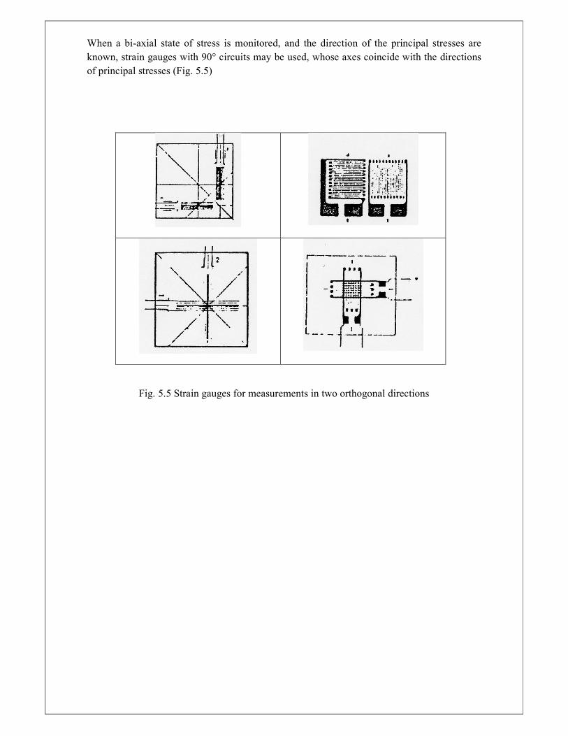
5.5 Wheastone bridge
The Wheatstone bridge is an electrical circuit consisting of four resistors configured in a
diamond-like arrangement, with two input terminals (A, B = E0) and two output terminals (C,
D = V) as shown in figure 5.7.
Fig. 5.7 Wheatstone bridge
Using Ohm and Kirchhoff laws, the output voltage can be written function of the input voltage
and R1-R4:
V = E0 (R2 R4 – R1 R3) / (R1 + R2) (R3 + R4)
The bridge is balanced when the voltage is zero, ie the situation in which:
R1R3 = R2 R4
This equality is verified for the particular case in which all four resistances are equal.
The variation of the resistances gives a variation of the output voltage measured at C, D
terminals:
∆V = E0 (∆R1/R1 -∆R2/R2 + ∆R3/R3 - ∆R4/R4) / 4
Consequently, if one of the resistances varies, the unbalanced voltage is proportional to the
relative variation of this resistance.

If one of the resistors is replaced by a strain gauge, it is possible, in this way, to measure its
resistance variation.
Before beginning the test, the bridge must be balanced, this being done automatically by
modern data acquisition systems, by varying the resistances of the other resistors included in
the bridge (R1 = R2 = R3 = R4).
Changes in output voltage is proportional to the supply voltage, the latter must therefore be
perfectly stabilized.
5.5.1 Quarter-bridge configuration
The quarter-bridge configuration means that only one resistor in one arm of the bridge is
replaced by a strain gauge (eg R1).
The variation of the output voltage may be written:
∆V = E0 (∆R1/R1 +/- 0 ) / 4= E0 ∆R1/R1 / 4 = E0 ∆R1 / 4 R1
The data acquisition system automatically calculates the variation of the resistance and of the
output voltage, providing directly the strain value in µs.
The wiring is made typically using three wires, as shown in Figure 5.8, to eliminate the effect
of temperature on resistance of the connection cable (it will be explained latter in this chapter).
Fig. 5.8 Quarter-bridge configuration/ three-wires
5.5.2 Half-bridge configuration
Considering this configuration, the difference of the signals provided by two strain gauges may
be monitored. The two strain gauges may be installed in two adjacent branches of the bridge,
for instance R1 and R2 such that:
∆V = E0 (∆R1 / R1 - ∆R2 / R2) / 4
This type of configuration is used mainly to eliminate the parasite effects that can influence the
main strain gauge R1. The gauge corresponding to resistor R2 will be placed in the same
conditions as R1, stuck on the same material, but without being subjected to mechanical load.

If the variation of the resistance R1 contains parasitic effects that overlaps the signal due to
mechanical load, the variation of the resistance R2 will be equal to this value:
∆R2 = ∆Rp
and
∆V = E0 [(Kε + ∆Rp / R) - ∆Rp / R] / 4 = E0 Kε / 4
The ‘compensation’ strain gauge was classically the best way to eliminate the parasite effects
of the temperature. This practice was generally eliminated, considering ‘auto-compensated’
strain gauges, specially designed for the specific material to be tested. These gauges are made
of special alloys, and are able to follow the thermal elongation of the tested specimen.
Half-bridge configuration may be used in particular circumstances when the two gauges
provide the same measurement values but with opposite signs and thus the mean value of the
measurement may be obtained.
For instance, for a simply supported steel beam in bending, one of the strain gauges may be
placed on the top flange (R2) and the other one on the bottom flange (R1), on the same vertical
axis. If the beam is subjected to vertical loads, the lower flange is in tension, while the upper
flange is in compression, so the values of the strains are the same, but with opposite signs.
Considering the equations for half-bridge configuration, the signals from R1 and R2 will be
finally added. However, any parasite effect (eg thermal elongation of the beam) will be added
in R1, but decreased in R2. The advantage of this configuration is that is insensitive to parasite
effects; however, there is a risk of getting incorrect results in case of malfunction of one of the
gauges.
In half-bridge configuration, the wiring is done considering two wires for each gauge.
5.6 Parasite effects occurring in strain measurement
5.6.1 Wheatstone bridge non-linearity
The equations above were obtained neglecting second order terms of resistance variations.
These expressions are therefore valid for small strains, but presents a risk if the strains are
important, for instance in the plastic domain.
Considering the quarter-bridge configuration, the relative error of voltage variation versus the
value computed by neglecting second order terms is (for a calibration factor K = 2):
e = [ε / (1+ ε)] x 100 [%]
For a strain of 1%, the relative error is of 1%. This corresponds to an elongation exceeding the
elastic limit of the steel, for instance (about 0.2% strain). The error will therefore neglectable
for testing in the elastic domain.
For a strain of 10%, however, the error obtained is 9.1%, which becomes unacceptable. The
only way to correct the nonlinearity of the bridge is by calculation.
The non-linearity may be canceled by a half-bridge configuration, when measuring two equal
strains of opposite signs, as in the example of steel beam in bending presented above.
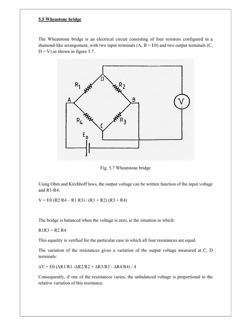
5.6.2 The effect of cable length on the total resistance
When strain gauges are located far away from the data acquisition system it is necessary to take
into account the resistance of the cables, due to their length.
The gauge calibration factor given by the manufacturer is:
K = (∆R / R1) / ε
in which R1 is the resistance of the strain gauge.
If the gauge is connected by very long cables, their resistance RL will be in series in the
Wheastone bridge, thus the calibration factor becomes:
K’ = [∆R / (R1+ RL )] / ε < K
Therefore, in case of long cables, a correction factor is required for the calibration factor. This
can be computed as shown in Figure 5.9.
Fig. 5.9 Calibration factor correction
5.6.3 Effect of temperature on the resistance of the connecting cables
Variation of the resistance of the connecting cables due to temperature is added to the variation
of the resistance of the strain gauge (due to mechanical loading), leading to inaccurate measures.

This effect is eliminated by a particular connection of strain gauge within the quarter-bridge
configuration, using three-wires, as shown in Fig. 5.8.
If the wires 1, 2 and 3 have the same length, it may be observed that the active branch contains
two lengths (1 and 2) in series with the strain gauge, while the adjacent branch also contains
two lengths (2 and 3) in series with the resistance R2. Consequently, a temperature variation
translates into an equal variation of the resistances in the two branches and therefore are
compensated, considering the equation of the output voltage ∆V in the Wheatstone bridge.
5.8 Fixation of the strain gauges on the tested specimen
This issue is particularly important, and requires special treatment of the surface on that the
strain gauge will be fixed. Figure 5.10 presents the steps needed to perform this operation.
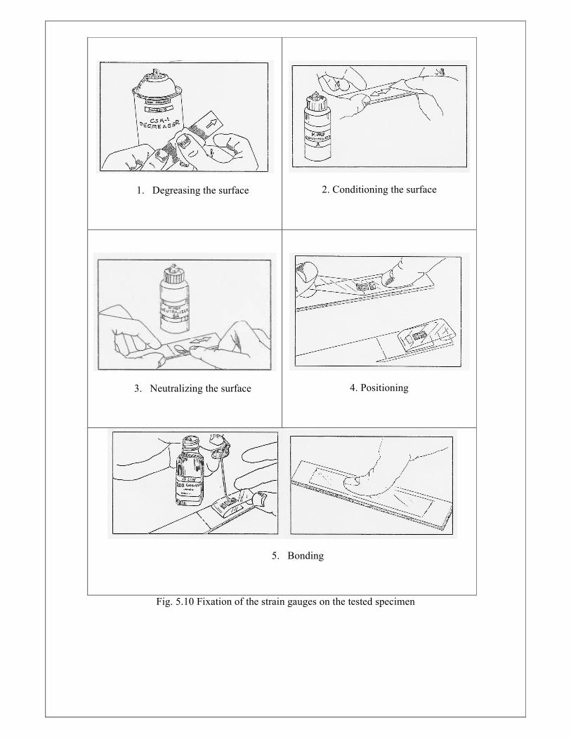
1. Degreasing the surface
2. Conditioning the surface
3. Neutralizing the surface
4. Positioning
5. Bonding
Fig. 5.10 Fixation of the strain gauges on the tested specimen

6. Load cells
6.1 Operating principle
A load cell is a transducer that is used to create an output signal whose magnitude is directly
proportional to the force being measured. The various types of load cells include hydraulic load
cells (the forces are measured using pressure), displacement-based load cells (forces measured
by calibrating the displacement of a spring) and deformation-based load cells (through a
mechanical arrangement, the force to be measured deforms a strain gauge).
Deformation-based load cells using strain gauges are the most common. The strain gauges are
bonded onto a specimen (usually of steel) inside the load cell, which deforms when the force
to be measured is applied. The change in resistance of the strain gauge provides an electrical
value change that is calibrated to the load placed on the load cell, see fig. 6.1.
Fig. 6.1 Load cell based on deformation
The advantages of this type of load cells are:
• low size and mass;
• robustness and high reliability as gauges are bonded on specimens of steel, which makes a
compact device, shockproof;
• high stability (the ability to retain calibration over a long period of time, in terms of fair use);
• reduced sensitivity to external factors by placing the gauges in appropriate configurations on
the steel specimen inside the load cell and within the Wheastone bridge circuit.
In a given section of the specimen inside the load cell, the load to be measured may produce
an axial force, two shear forces, two bending moments and a torque. The basic idea is that the
shape of the specimen and the location and orientation of the gauges should be chosen in such
a way to allow for the measurement of a single internal force which will generate the strain/
signal to be measured. Thus, the load cells may be constructed based on a deformation from an
axial force (Fig. 6.2.a), a bending moment (Fig. 6.2.b) or a shear force (Fig. 6.2.c).

Fig. 6.2 Load cell based on deformation from (a) axial force
(b) bending moment (c) shear force
6.2 Load cells based on deformation from bending moment
Let’s realize a load cell based on deformation from bending moment.
As shown in Figure 6.3, we consider a cantilever with steel cross-section (e x b) at the end of
which the load to be measured (P) is applied.
Fig. 6.3 Construction of a load cell
The simplest solution is to bond a strain gauge (labeled '1 'in the figure 6.3) at a distance a from
the application point of the load, far enough from the fixed support in order to avoid
perturbations. This gauge will be placed on R1 branch of the Wheastone bridge (quarter-bridge).
The strain measured by the gauge function of the load is:
ε1 = σ / E = M / E W = 6Pa / Ebe2
(M = P a; W = be2 / 6)
The output voltage of the Wheastone bridge is:

∆V = E0 ε1 K / 4
To remove various parasite signals a second gauge (labeled ‘2’ in figure 6.3) may be placed
under gauge ‘1’, and placed on the R2 branch in the Wheastone bridge (half-bridge).
Parasite effects are thus eliminated, because the gauges occupy adjacent branches in the bridge,
and parasite signals will cancel each other. The relationship between voltage and strain
variation can be written:
∆V = E0 [K ε1 – (-K ε1) ] / 4 = 2 E0 K ε1 / 4
The output is thus became twice as sensitive for measuring the effect of force P and is
insensitive to various parasite signals.
Gauges labeled ‘3’ and ‘4’ in figure 6.3 may be bonded on the specimen, and introduced in
branches R3 and R4 of the bridge, respectively. Thus the output become four times more
sensitive (compared with considering only one gauge) for measuring the effect of the force P
and is still insensitive to various parasite signals:
∆V = 4 E0 K ε1 / 4 = E0 K ε1
This represents the full-bridge configuration, which is usually considered for load cells, in order
to use at maximum the branches of the Wheastone bridge.
Instead of a cantilever specimen, a fixed specimen may be considered, as shown in figure 6.4.
Fig. 6.4 Load cell based on deformation from bending moment
Gauges in tension and compression are labeled respectively by 'T' and 'C' and have the same
values of the strain, but with opposite signs. Gauges in tension will be wired on R1 and R3
branches on the Wheatstone bridge, while the gauges in tension will be wired on R2 and R4
branches. A problem of this arrangement is that, in case of large displacements, nonlinearities
occur in the sensor operation, the bending moments of force P in relation to the location of the
gauges being thus different.
To obtain strains that are equal for T and C a variant of the specimen is presented in figure 6.5.
This configuration may be found in modern load cells based on deformation from bending
moment, as shown in figure 6.5, through an arrangement in which the gauges are bonded on
two branches, or inside a hole.
Fig. 6.5 Modern load cell based on deformation from bending moment
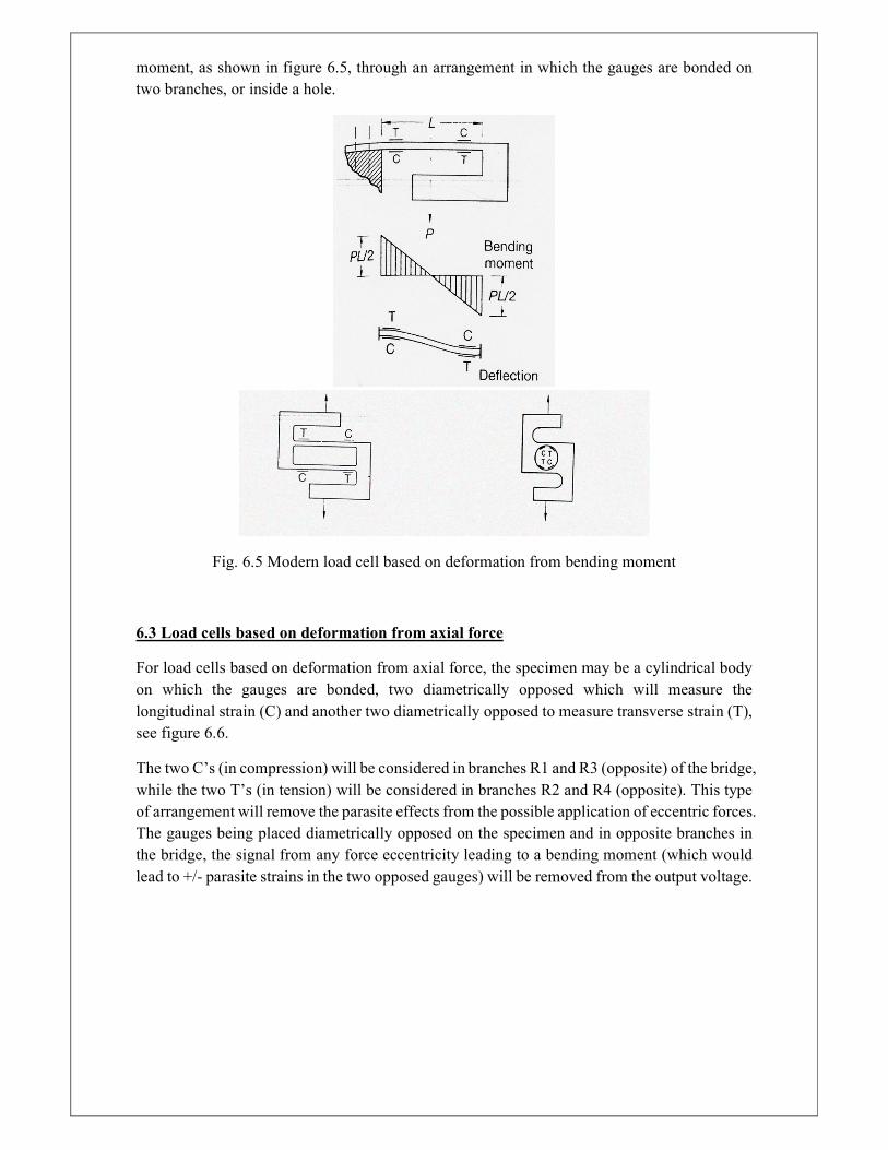
6.3 Load cells based on deformation from axial force
For load cells based on deformation from axial force, the specimen may be a cylindrical body
on which the gauges are bonded, two diametrically opposed which will measure the
longitudinal strain (C) and another two diametrically opposed to measure transverse strain (T),
see figure 6.6.
The two C’s (in compression) will be considered in branches R1 and R3 (opposite) of the bridge,
while the two T’s (in tension) will be considered in branches R2 and R4 (opposite). This type
of arrangement will remove the parasite effects from the possible application of eccentric forces.
The gauges being placed diametrically opposed on the specimen and in opposite branches in
the bridge, the signal from any force eccentricity leading to a bending moment (which would
lead to +/- parasite strains in the two opposed gauges) will be removed from the output voltage.

Fig. 6.6 Specimen of load cell based on deformation from axial force
A cross-section of such a load cell is presented in figure 6.7.
Fig. 6.7 Load cell based on deformation from axial force
High capacity load cells can be built with four or more prismatic or cylindrical specimens in
parallel, as shown in Figure 6.8.
As a general rule, low and medium intensity forces are measured using load cells based on
deformation from bending moment, while for high intensity forces load cells based on
deformation from axial force are considered.

Fig. 6.8 High capacity load cells
BIBLIOGRAPHY
Analyse experimentale et numerique de modeles reduits en vibration. These fin d’etudes,
Cedric Stewart, Faculte des Sciences Appliquees, Universite de Liege, Belgia, 1996-1997.
Coordonatori: Prof. G. FonderFonder G., Boeraeve M
Encyclopedie d`analyse des contraintes, J. Avril, Ed. Micromesures, Malakoff, Franta, 1983
Handbook of experimental analysis. Mindin RD, Salvadori MG, Ed. Wiley & Sons, New York,
1984
Handbook on structural testing, R. T. Reese, W. A. Kawahara, The Fairmont Press Inc., 1993
Introducere in tehnica proiectării asistate de experiment a construcţiilor metalice, M.
Georgescu, R. Zaharia, Ed. Orizonturi Universitare, Timisoara, 1999
Manuel du laboratoire de resistence des materiaux ; Notes de cours redigees par J. Rondal,
M. Braham, S. Cescotto, R. Maquoi. Faculte des Sciences Appliquees, Universite de Liege,
Belgium, 1980.
Techniques experimentales modernes pour la conduite et exploitation d’essais de structures en
genie civil, A. Lachal, Laboratoire des Structures INSA – Rennes, France, 1994
Theory and design for mechanical measurements, R. S. Figliola, D. E. Beasley, John Wiley &
Sons, Inc., 1994 (second edition)
Theory and practice of force measurement - Monographs in physical measurement - A. Bray,
Giulio Barbato, Raffaello Levi Academic Press, University of California, 1990
Wikipedia – The Free Encyclopedia: http://en.wikipedia.org