1

Design and Prototyping Methods for Brushless Motors and Motor Control

by

Shane W. Colton

B.S., Mechanical Engineering (2008)

Massachusetts Institute of Technology

Submitted to the Department of Mechanical Engineeringin Partial Fulfillment of the Requirements for the Degree of

Master of Science in Mechanical Engineering

at the

Massachusetts Institute of Technology

June 2010

© Massachusetts Institute of TechnologyAll rights reserved

Signature of Author . . . . . . . . . . . . . . . . . . . . . . . . . . . . . . . . . . . . . . . . . . . . . . . . . . . . . . . . . . . . . Department of Mechanical Engineering

May 7, 2010

Certified by . . . . . . . . . . . . . . . . . . . . . . . . . . . . . . . . . . . . . . . . . . . . . . . . . . . . . . . . . . . . . . . . . . . . Daniel Frey

Associate Professor of Mechanical Engineering and Engineering SystemsThesis Supervisor

Accepted by . . . . . . . . . . . . . . . . . . . . . . . . . . . . . . . . . . . . . . . . . . . . . . . . . . . . . . . . . . . . . . . . . . . David E. Hardt

Ralph E. & Eloise F. Cross Professor of Mechanical EngineeringChairman, Department Committee on Graduate Students

2

3

Design and Prototyping Methods for Brushless Motors and Motor Control

by

Shane W. Colton

Submitted to the Department of Mechanical Engineeringon May 7, 2010 in partial fulfillment of the

requirements for the Degree of Master of Science in Mechanical Engineering

ABSTRACT

In this report, simple, low-cost design and prototyping methods for custom brushless permanent magnet synchronous motors are explored. Three case-study motors are used to develop, illustrate and validate the methods. Two 500W hub motors are implemented in a direct-drive electric scooter. The third case study, a 10kW axial flux motor, is used to demonstrate the flexibility of the design methods. A variety of ways to predict the motor constant, which relates torque to current and speed to voltage, are presented. The predictions range from first-order DC estimates to full dynamic simulations, yielding increasingly accurate results. Ways to predict winding resistance, as well as other sources of loss in motors, are discussed in the context of the motor’s overall power rating. Rapid prototyping methods for brushless motors prove to be useful in the fabrication of the case study motors. Simple no-load evaluation techniques confirm the predicted motor constants without large, expensive test equipment.

Methods for brushless motor controller design and prototyping are also presented. The case study, a two channel, 1kW per channel brushless motor controller, is fully developed and used to illustrate these methods. The electrical requirements of the controller (voltage, current, frequency) influence the selection of components, such as power transistors and bus capacitors. Mechanical requirements, such as overall dimensions, heat transfer, and vibration tolerance, also play a large role in the design. With full-system prototyping in mind, the controller integrates wireless data acquisition for debugging. Field-oriented AC control is implemented on low-cost hardware using a novel modification of the standard synchronous current regulator. The controller performance is evaluated under load on two case study systems: On the direct-drive electric scooter, it simultaneously and independently controls the two motors. On a high-performance remote-control car, a more extreme operating point is tested with one motor.

Thesis Supervisor: Daniel Frey

Title: Associate Professor of Mechanical Engineering and Engineering Systems

4

Table of Contents1 Introduction............................................................................................................................. 6

1.1 Project Motivation .......................................................................................................... 61.2 Acknowledgments........................................................................................................... 7

2 Fundamentals and Relevant Physical Principles..................................................................... 82.1 Brushless Motor Terminology and Types....................................................................... 8

2.1.1 Basic Terminology.................................................................................................. 82.1.2 Motor Model, Back EMF, Motor Constant .......................................................... 102.1.3 Resistance, Inductance, Saliency, and Field Weakening...................................... 12

2.2 DC vs. AC: Back EMF, Drive, and Torque Production ............................................... 132.2.1 Trapezoidal vs. Sinusoidal Back EMF.................................................................. 142.2.2 Square Wave vs. Sine Wave Drive ....................................................................... 152.2.3 Torque Production Comparison............................................................................ 172.2.4 Mixed Back EMF / Drive ..................................................................................... 192.2.5 DC vs. AC Summary ............................................................................................ 21

2.3 Field-Oriented Control.................................................................................................. 222.3.1 d-q Reference Frame............................................................................................. 222.3.2 Vector Motor Quantities ....................................................................................... 232.3.3 Why Control is Necessary: Motor Inductance...................................................... 262.3.4 Field-Oriented Control Objective ......................................................................... 282.3.5 Synchronous Current Regulator............................................................................ 29

3 Brushless Motor Design and Prototyping Methods .............................................................. 313.1 Design Strategy and Goals............................................................................................ 313.2 Introduction of Case Studies......................................................................................... 32

3.2.1 Direct-Drive Kick Scooter Motors........................................................................ 323.2.2 Axial Flux Motor .................................................................................................. 34

3.3 Motor Constant: Various Prediction Methods .............................................................. 413.3.1 First-Order Analysis: DC...................................................................................... 413.3.2 First-Order Analysis: Sinusoidal........................................................................... 463.3.3 2D Finite Element: Static...................................................................................... 483.3.4 2D Finite Element: Dynamic ................................................................................ 52

3.4 Resistance, Losses, and Power Rating.......................................................................... 553.4.1 I² Losses: Winding Resistance, Power Ratings .................................................... 563.4.2 E² Losses: Delta Windings, Eddy Current, and Mechanical Losses..................... 59

3.5 Motor Prototyping Methods.......................................................................................... 623.5.1 Integrated CAD/FEA/CAM.................................................................................. 623.5.2 Design for Assembly (and Disassembly).............................................................. 65

3.6 Evaluating Motor Performance..................................................................................... 673.6.1 Single-Phase Back EMF Testing .......................................................................... 683.6.2 Full-Motor Testing................................................................................................ 69

4 Motor Control Design and Prototyping Methods ................................................................. 714.1 Design Strategy and Goals............................................................................................ 714.2 Introduction of Case Study ........................................................................................... 724.3 Controller Design.......................................................................................................... 73

4.3.1 MOSFETs ............................................................................................................. 734.3.2 Bus Capacitors ...................................................................................................... 82

5

4.3.3 Power Supplies...................................................................................................... 854.3.4 Signal Filtering...................................................................................................... 87

4.4 Controller Layout and Mechanical Design ................................................................... 874.4.1 Power/Signal Isolation .......................................................................................... 874.4.2 Mechanical Constraints and Design...................................................................... 88

4.5 Field-Oriented Control Strategy ................................................................................... 934.5.1 Control Overview.................................................................................................. 934.5.2 Hall Effect Sensor Interpolation for Rotor Position ............................................. 934.5.3 Modified Synchronous Current Regulator............................................................ 96

4.6 Data Acquisition and Analysis...................................................................................... 994.6.1 Integrated Wireless Data Acquisition ................................................................... 994.6.2 Data Visualization/Analysis: Real Time and Post-Processed............................. 100

4.7 Evaluating Controller Performance ............................................................................ 1014.7.1 Direct-Drive Scooter Motors .............................................................................. 1014.7.2 RC Car Motor ..................................................................................................... 105

5 Conclusions......................................................................................................................... 1086 References........................................................................................................................... 1097 Appendices.......................................................................................................................... 110

7.1 Modular, Optically-Isolated Half-Bridge.................................................................... 1107.1.1 MOSFETs ........................................................................................................... 1117.1.2 Optocouplers ....................................................................................................... 1137.1.3 Drive Signal Inverter........................................................................................... 1147.1.4 DC/DC Converter (High-Side Supply)............................................................... 1147.1.5 Full Half-Bridge.................................................................................................. 1157.1.6 Controlling the Half-Bridge................................................................................ 118

7.2 Schematic of Case Study Controller ........................................................................... 1207.3 Source Code of Case Study Controller ....................................................................... 125

7.3.1 lookups.h............................................................................................................. 1257.3.2 main.c.................................................................................................................. 125

6

1 Introduction

1.1 Project MotivationElectric motors are one of the key elements of mechanical design, used in many applications ranging from toys to propulsion of full-scale vehicles. Few if any simpler ways exist to produce torque and rotary motion; most electric motors have a single moving part. Thanks in large part to this simplicity, electric motors also have a high-fidelity electromechanical model. This model can be used to accurately predict motor and full-system performance. A thorough understanding of this model is useful whether selecting a motor from a catalog or designing one from scratch.

Brushless permanent magnet synchronous motors (PMSM) are increasingly replacing brushed DC motors in low- to medium-power servo applications. In these motors, electronic commutation is used in lieu of mechanical brushes. This reduces friction, increases reliability, and decreases the cost to produce the motor itself. The tradeoff is more complex and expensive controllers. However, the economies of scale of electrical components are very different than those of the motors themselves, and a system-wide cost/performance evaluation favors brushless motors in many applications.

For the author, brushless motors present an interesting educational opportunity as well. Specifically, they can be designed, built, and tested without the need for special tools thanks to their simplicity. Using the motor model, a first-order analysis can predict the motor’s performance to good accuracy. Free simulation tools for electromagnetic finite element analysis [1] can yield even better predictions. Without a brush and commutator assembly, the only mechanical element that cannot be made with standard machining capability is the laminated stator core. Rapid prototyping, in the form of laser cutting, can produce this part with no tooling cost. In other cases, existing stator cores can be bought or salvaged if they fit the design. Hand-winding and magnet placement is possible and effective for smaller motors.

The opportunity to explore brushless motors first presented itself in the form of a project carried out during the summer of 2009. As part of the Edgerton Center’s Summer Engineering Workshop [2,3], the author led a team of students to produce a direct-drive kick scooter using custom brushless hub motors. These motors are introduced as case studies in Section 3.2.1. A thorough understanding of the motor model was developed throughout this project. At the same time, many of the practical issues in implementing a real motor design came up. The opportunity for a significant design study was apparent. A second case-study motor, originally designed for an electric motorcycle, was developed as part of this design study. This motor, a larger axial-flux configuration, has a very different topology but can be analyzed in much the same way, demonstrating the flexibility of the design methods.

After completing the motor design and fabrication for the direct-drive scooter with the Summer Engineering Workshop, the author pursued a more advanced control method. Like many inexpensive brushless motors, the scooter hub motors used Hall effect sensors and square-wave commutation, typically referred to as brushless DC since it mimics the function of a brush and commutator. Using sinusoidal AC control, even on motors designed for brushless DC, offers

7

advantages such as quieter/smoother operation and higher controller efficiency. Mechanical considerations such as poor thermal management and vibration tolerance also made the original brushless DC scooter controller less than ideal. The controller presented in Section 4 was originally designed to solve specific problems with the first scooter controller. However, it also demonstrates the extension of full sinusoidal AC motor control to low-cost hardware. It uses the existing Hall effect sensors and interpolation in lieu of more expensive position feedback devices. It is also optimized to run on low-speed fixed-point microprocessors.

All of the motor and controller design and testing and most of the fabrication for this study weredone in-house using only standard, commonly-available tools and equipment. This is effective proof that it is possible to do in-house motor and controller design even in labs for which that is not the primary focus. This obviously has its limits: building a full-scale vehicle motor or controller is likely beyond the capability of most individuals or labs. But for low- to medium-power applications, it is possible to design and develop custom motor and motor control solutions in-house. The methods presented in this report put emphasis on low cost and short design cycle time; rapid prototyping for motors. Admittedly, specialized research and development in electric machines goes much further than what is presented in this report. The goal here will be to illustrate a simple motor and controller design and prototyping process that could fit into a higher-level system design.

1.2 AcknowledgmentsThe author would like to thank Professor Daniel Frey for supervising this project. Very few advisors would be willing to give as much freedom and trust to explore a design as Dan does, and this project would not have been possible without his support.

The author would also like to thank the Edgerton Center and the Summer Engineering Workshop crew for continuing to provide a source of interesting projects and a fun place to work. The opportunity to combine technical study with educational and teaching opportunity is something that is unique and much appreciated.

The author would like to thank Charles Guan ’11 for providing inspiration and technical support for the projects, particularly the direct drive electric scooter.

The author would like to thank the MIT Electric Vehicle Team for providing opportunities to do interesting research on traction motors. In particular, thanks to Lennon Rodgers for his support of the axial flux motor project, as well as for his general technical knowledge and guidance.

The author would like to thank Proto Laminations, Inc, for providing laser-cut laminations at no cost for the scooter motors, as well as the Electric Motor Education and Research Foundation for supporting an enlightening trip to the SMMA Fall Technical Conference. In particular, the author would like to thank Steve Sprague for his personal involvement in the project and commitment to electric motor education and research.

8

2 Fundamentals and Relevant Physical PrinciplesThis section will first cover some brushless motor terminology and taxonomy, and then outline some fundamental physical principles that will be relevant to the rest of the report. A full coverage of electric machine theory is beyond the scope of this report. See [4] for more background on electric machine theory and [5] for more background on motor control.

2.1 Brushless Motor Terminology and TypesIn more precise terminology, this report focuses on permanent magnet synchronous motors (PMSM). These are motors in which permanent magnets on the rotor create a magnetic field which interact with synchronous stator current. “Synchronous” simply means that the electrical and mechanical frequencies are linked. There is no “slip” as there would be in an AC induction motor.

For brevity, the term “brushless motor” is used in this report to mean “permanent magnet synchronous motor.” AC induction motors, and other motors that technically don’t have brushes, are not included in this classification. However, the term is not restricted to brushless DC (BLDC). Thus, it also includes other common motor classifications such as permanent magnet AC (PMAC) and brushless AC (BLAC). The technical difference between DC and AC permanent magnet synchronous motors is a common point of confusion, addressed in Section 2.2.

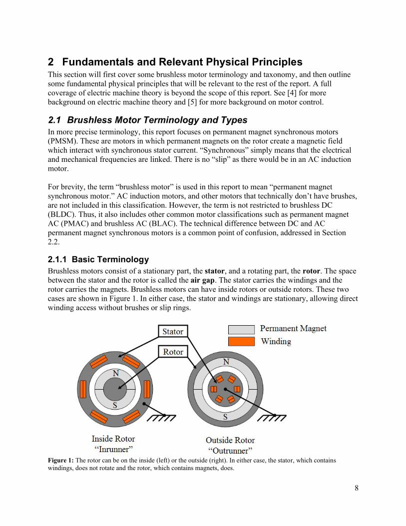
2.1.1 Basic TerminologyBrushless motors consist of a stationary part, the stator, and a rotating part, the rotor. The space between the stator and the rotor is called the air gap. The stator carries the windings and the rotor carries the magnets. Brushless motors can have inside rotors or outside rotors. These two cases are shown in Figure 1. In either case, the stator and windings are stationary, allowing direct winding access without brushes or slip rings.

Figure 1: The rotor can be on the inside (left) or the outside (right). In either case, the stator, which contains windings, does not rotate and the rotor, which contains magnets, does.

9

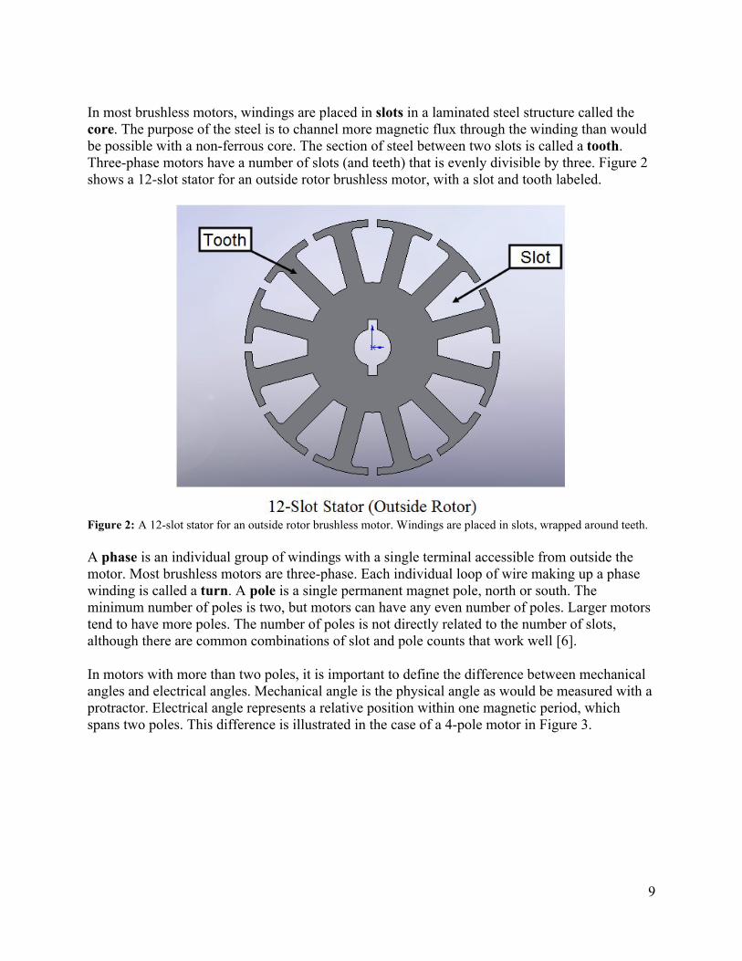
In most brushless motors, windings are placed in slots in a laminated steel structure called the core. The purpose of the steel is to channel more magnetic flux through the winding than would be possible with a non-ferrous core. The section of steel between two slots is called a tooth. Three-phase motors have a number of slots (and teeth) that is evenly divisible by three. Figure 2shows a 12-slot stator for an outside rotor brushless motor, with a slot and tooth labeled.

Figure 2: A 12-slot stator for an outside rotor brushless motor. Windings are placed in slots, wrapped around teeth.

A phase is an individual group of windings with a single terminal accessible from outside the motor. Most brushless motors are three-phase. Each individual loop of wire making up a phase winding is called a turn. A pole is a single permanent magnet pole, north or south. The minimum number of poles is two, but motors can have any even number of poles. Larger motors tend to have more poles. The number of poles is not directly related to the number of slots, although there are common combinations of slot and pole counts that work well [6].

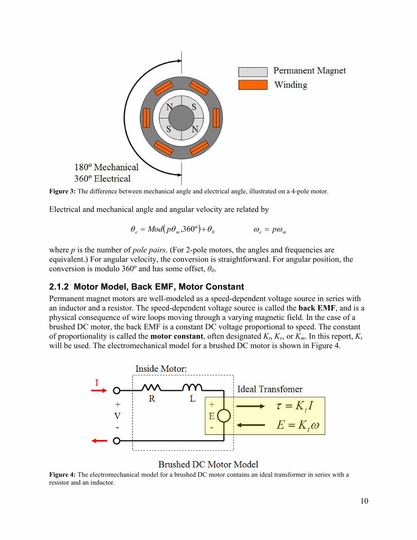
In motors with more than two poles, it is important to define the difference between mechanical angles and electrical angles. Mechanical angle is the physical angle as would be measured with a protractor. Electrical angle represents a relative position within one magnetic period, which spans two poles. This difference is illustrated in the case of a 4-pole motor in Figure 3.

10

Figure 3: The difference between mechanical angle and electrical angle, illustrated on a 4-pole motor.

Electrical and mechanical angle and angular velocity are related by

0º360, me pMod me p

where p is the number of pole pairs. (For 2-pole motors, the angles and frequencies are equivalent.) For angular velocity, the conversion is straightforward. For angular position, the conversion is modulo 360º and has some offset, θ0.

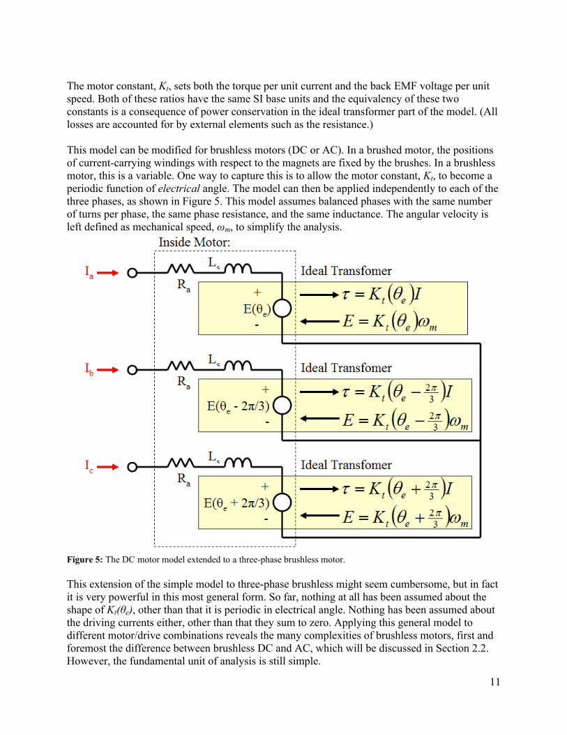
2.1.2 Motor Model, Back EMF, Motor ConstantPermanent magnet motors are well-modeled as a speed-dependent voltage source in series with an inductor and a resistor. The speed-dependent voltage source is called the back EMF, and is a physical consequence of wire loops moving through a varying magnetic field. In the case of a brushed DC motor, the back EMF is a constant DC voltage proportional to speed. The constant of proportionality is called the motor constant, often designated Kt, Kv, or Km. In this report, Kt

will be used. The electromechanical model for a brushed DC motor is shown in Figure 4.

Figure 4: The electromechanical model for a brushed DC motor contains an ideal transformer in series with a resistor and an inductor.

11

The motor constant, Kt, sets both the torque per unit current and the back EMF voltage per unit speed. Both of these ratios have the same SI base units and the equivalency of these two constants is a consequence of power conservation in the ideal transformer part of the model. (All losses are accounted for by external elements such as the resistance.)

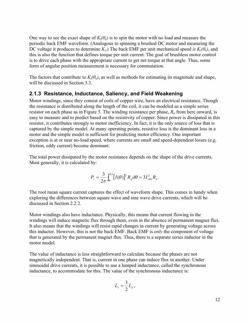
This model can be modified for brushless motors (DC or AC). In a brushed motor, the positions of current-carrying windings with respect to the magnets are fixed by the brushes. In a brushless motor, this is a variable. One way to capture this is to allow the motor constant, Kt, to become a periodic function of electrical angle. The model can then be applied independently to each of the three phases, as shown in Figure 5. This model assumes balanced phases with the same number of turns per phase, the same phase resistance, and the same inductance. The angular velocity is left defined as mechanical speed, ωm, to simplify the analysis.

Figure 5: The DC motor model extended to a three-phase brushless motor.

This extension of the simple model to three-phase brushless might seem cumbersome, but in fact it is very powerful in this most general form. So far, nothing at all has been assumed about the shape of Kt(θe), other than that it is periodic in electrical angle. Nothing has been assumed about the driving currents either, other than that they sum to zero. Applying this general model to different motor/drive combinations reveals the many complexities of brushless motors, first and foremost the difference between brushless DC and AC, which will be discussed in Section 2.2. However, the fundamental unit of analysis is still simple.

12

One way to see the exact shape of Kt(θe) is to spin the motor with no load and measure the periodic back EMF waveform. (Analogous to spinning a brushed DC motor and measuring the DC voltage it produces to determine Kt.) The back EMF per unit mechanical speed is Kt(θe), and this is also the function that defines torque per unit current. The goal of brushless motor control is to drive each phase with the appropriate current to get net torque at that angle. Thus, some form of angular position measurement is necessary for commutation.

The factors that contribute to Kt(θe), as well as methods for estimating its magnitude and shape, will be discussed in Section 3.3.

2.1.3 Resistance, Inductance, Saliency, and Field WeakeningMotor windings, since they consist of coils of copper wire, have an electrical resistance. Though the resistance is distributed along the length of the coil, it can be modeled as a simple series resistor on each phase as in Figure 5. The winding resistance per phase, Ra from here onward, is easy to measure and to predict based on the resistivity of copper. Since power is dissipated in this resistor, it contributes strongly to motor inefficiency. In fact, it is the only source of loss that is captured by the simple model. At many operating points, resistive loss is the dominant loss in a motor and the simple model is sufficient for predicting motor efficiency. One important exception is at or near no-load speed, where currents are small and speed-dependent losses (e.g. friction, eddy current) become dominant.

The total power dissipated by the motor resistance depends on the shape of the drive currents. Most generally, it is calculated by:

armsar RIdRIP 22

0

2 3)(2

3

.

The root mean square current captures the effect of waveform shape. This comes in handy when exploring the differences between square wave and sine wave drive currents, which will be discussed in Section 2.2.2.

Motor windings also have inductance. Physically, this means that current flowing in the windings will induce magnetic flux through them, even in the absence of permanent magnet flux. It also means that the windings will resist rapid changes in current by generating voltage across this inductor. However, this is not the back EMF. Back EMF is only the component of voltage that is generated by the permanent magnet flux. Thus, there is a separate series inductor in the motor model.

The value of inductance is less straightforward to calculate because the phases are not magnetically independent. That is, current in one phase can induce flux in another. Under sinusoidal drive currents, it is possible to use a lumped inductance, called the synchronous inductance, to accommodate for this. The value of the synchronous inductance is:

as LL2

3 ,

13

where La is the inductance that would be measured independently on one phase, if it could be isolated. This is derived in [4]. For the purposes of this report, some lumped inductance per phase, Ls, will be assumed even for non-sinusoidal drive currents.

The winding inductance has many theoretical and practical effects on the motor. It stores energy in the form of a magnetic field any time there is current in the winding. When a winding is switched off, this energy must go somewhere. For this reason, controllers contain “flyback diodes” that allow this current to circulate even when all the switches are open. Under high frequency pulse-width modulated (PWM) control, the winding inductance also filters out current ripple. However, as a low-pass filter on current it also creates phase lag. This lag is explored in detail in Section 2.3.3 as motivation for the use of field-oriented control.

The winding inductance is a function of motor geometry and the number of turns in the winding. In non-salient motors, also called round rotor, the inductance is not a function of electrical angle. This is the case for motors with complete radial symmetry of the rotor’s steel backing at any angle. (The magnets themselves don’t matter, since they have nearly the same permeability as air.) Motors with magnets mounted to the surface of the rotor steel, called surface permanent manget (SPM), fall into this category. Salient motors have an inductance that varies periodically with electrical angle. This is the case if the rotor’s steel backing is different at the poles than in between them. Motors with magnets embedded in the steel backing, called interior permanent magnet (IPM), fall into this category. This report will focus exclusively on non-salient, SPM motors. Torque production for salient motors requires a slightly more complicated analysis.

Motor inductance also has a large effect on field weakening, a technique usually used to extend the operating speed range of a motor. In field weakening, some current is used to induce a field which partially cancels the permanent magnet field. This results in less torque per unit current, but also decreases the back EMF per unit speed, allowing the motor to be operated to higher speeds with a given voltage. Field weakening will be explored further in Section 2.3.4 as a specific case of field-oriented control. In general, motors with lower inductance have less field-weakening capability.

2.2 DC vs. AC: Back EMF, Drive, and Torque ProductionThis section explores the differences (and similarities) between brushless DC motors and permanent magnet AC (PMAC) motors, also called permanent magnet synchronous motors (PMSM). The analysis itself is not complicated, but sorting out a consistent and unambiguous definition of the different motor types can be challenging. This is due, in large part, to the fact that both the motor and the drive are involved in the definition. The motor, and specifically the shape of its back EMF waveform (trapezoidal or sinusoidal), is only part of the story and must be matched with a drive strategy (square wave or sinusoidal) to form a complete definition. One of the most thorough approaches to this challenge is contained in the S.M. thesis of James Mevey [5]. To directly quote Mevey:

It is the author’s opinion that the difference between trap and sine [brushless motors] is surrounded by more misunderstanding and confusion than any other subject in the field of brushless motor control.

14

This section will first outline a consistent definition of the two types of motor, then look at torque production in each case. Finally, torque production in the mixed case of sinusoidal drive with a trapezoidal back EMF will be explored.

2.2.1 Trapezoidal vs. Sinusoidal Back EMFTo start tackling the problem, brushless motors themselves can be broken into two different types based on the shape of their back EMF: sinusoidal and trapezoidal. These are really just the extremes of a large spectrum of possible real motors. However, these two extremes will be used to bound the analysis.

The classification is based on the shape of the back EMF waveform of the motor, which is the voltage it produces at its terminals as a function of rotor position with no load. The amplitude of the back EMF is proportional to the angular velocity of the motor, but its shape will not change with speed. This relationship is completely captured by the following:

dt

dE r

rr

)(

Rotor flux linkage, λr, is a function of rotor angular position. Back EMF, E, is the rate of change of rotor flux linkage in the winding. Therefore, the amplitude of the back EMF waveform is a function of angular velocity and the shape is a function of angular position. Some factors influencing the shape are: magnet geometry, magnetization, stator core geometry, and winding distribution. These are all properties of the motor itself, and do not depend on the drive.

The two extreme shapes that are considered in this section are sinusoidal and trapezoidal. Figure 6 shows the ideal sinusoidal and trapezoidal back EMF waveforms. The ideal trapezoidal waveform has a 120º flat top for reasons that will become apparent when the drive strategy is explored. In order to keep the comparison “fair,” the amplitudes of the two back EMF waveforms are normalized such that they both have an RMS value of 1.

15

0 30 60 90 120 150 180 210 240 270 300 330 360-1.5

-1

-0.5

0

0.5

1

1.5

Rotor Electrical Angle (deg)

Nor

mal

ized

Bac

k E

MF

Sinusoidal

Trapezoidal

Figure 6: Ideal sinusoidal vs. trapezoidal back EMF waveforms, normalized to RMS=1.

Some physical conditions that would lead to a trapezoidal back EMF are: Concentrated windings. No stator or magnet skew. Discrete magnet poles with uniform magnetization.

These conditions all lead to sharp transitions in the flux linkage, which give the trapezoidal back EMF waveform its distinct shape. While it does influence the shape of the back EMF, stator core saturation is not the reason for the flat top of the back EMF. (Saturation implies small rate of change of flux, so it would affect the shape near the back EMF zero crossing, not at the peaks.)

Some physical conditions that would lead to a sinusoidal back EMF are as follows: Overlapped or sinusoidally-distributed windings. A coreless stator (with windings only, no steel laminations). Stator and/or magnet skew. Sinusoidal magnetization.

These conditions all round off the flux linkage so that it more closely approximates an ideal sinusoid. Practically, a motor with these characteristics can be more difficult to make, and thus more costly. In general, low-cost motors tend to have a more of the characteristics that lead to a trapezoidal back EMF.

2.2.2 Square Wave vs. Sine Wave DriveHow the motor is driven with currents also plays a role in whether it is considered DC or AC. Typically, motors with more trapezoidal back EMF are driven with six-step square wave commutation and are considered brushless DC. Motors with more sinusoidal back EMF are driven with three-phase sinusoidal commutation, and are considered AC. However, any back

16

EMF shape can be driven by either square wave or sine wave drive, and a mixed case will be explored in 2.2.4. First, a closer look at the two drive strategies is presented.

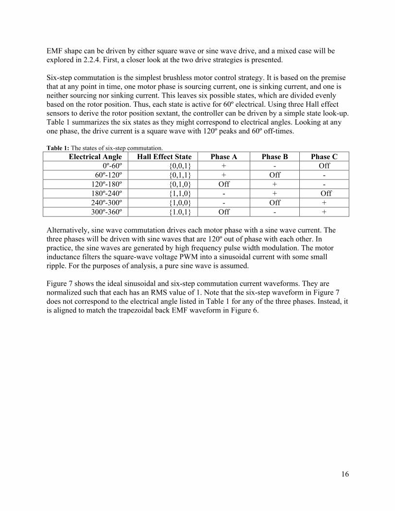
Six-step commutation is the simplest brushless motor control strategy. It is based on the premise that at any point in time, one motor phase is sourcing current, one is sinking current, and one is neither sourcing nor sinking current. This leaves six possible states, which are divided evenly based on the rotor position. Thus, each state is active for 60º electrical. Using three Hall effect sensors to derive the rotor position sextant, the controller can be driven by a simple state look-up. Table 1 summarizes the six states as they might correspond to electrical angles. Looking at any one phase, the drive current is a square wave with 120º peaks and 60º off-times.

Table 1: The states of six-step commutation.

Electrical Angle Hall Effect State Phase A Phase B Phase C0º-60º {0,0,1} + - Off

60º-120º {0,1,1} + Off -120º-180º {0,1,0} Off + -180º-240º {1,1,0} - + Off240º-300º {1,0,0} - Off +300º-360º {1.0,1} Off - +

Alternatively, sine wave commutation drives each motor phase with a sine wave current. The three phases will be driven with sine waves that are 120º out of phase with each other. In practice, the sine waves are generated by high frequency pulse width modulation. The motor inductance filters the square-wave voltage PWM into a sinusoidal current with some small ripple. For the purposes of analysis, a pure sine wave is assumed.

Figure 7 shows the ideal sinusoidal and six-step commutation current waveforms. They are normalized such that each has an RMS value of 1. Note that the six-step waveform in Figure 7does not correspond to the electrical angle listed in Table 1 for any of the three phases. Instead, it is aligned to match the trapezoidal back EMF waveform in Figure 6.

17

0 30 60 90 120 150 180 210 240 270 300 330 360-1.5

-1

-0.5

0

0.5

1

1.5

Rotor Electrical Angle (deg)

Nor

mal

ized

Driv

e C

urre

nt

Sinusoidal

Six-Step Square Wave

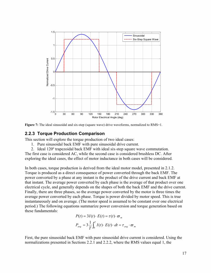
Figure 7: The ideal sinusoidal and six-step (square wave) drive waveforms, normalized to RMS=1.

2.2.3 Torque Production ComparisonThis section will explore the torque production of two ideal cases:

1. Pure sinusoidal back EMF with pure sinusoidal drive current.2. Ideal 120º trapezoidal back EMF with ideal six-step square wave commutation.

The first case is considered AC, while the second case is considered brushless DC. After exploring the ideal cases, the effect of motor inductance in both cases will be considered.

In both cases, torque production is derived from the ideal motor model, presented in 2.1.2. Torque is produced as a direct consequence of power converted through the back EMF. The power converted by a phase at any instant is the product of the drive current and back EMF at that instant. The average power converted by each phase is the average of that product over one electrical cycle, and generally depends on the shapes of both the back EMF and the drive current. Finally, there are three phases, so the average power converted by the motor is three times the average power converted by each phase. Torque is power divided by motor speed. This is true instantaneously and on average. (The motor speed is assumed to be constant over one electrical period.) The following equations summarize power conversion and torque generation based on these fundamentals:

mavg

T

avg

m

dttEtIT

P

ttEtItP

0 )()(1

3

)()()(3)(

First, the pure sinusoidal back EMF with pure sinusoidal drive current is considered. Using the normalizations presented in Sections 2.2.1 and 2.2.2, where the RMS values equal 1, the

18

calculation is easy. The normalized average power generated by the three phases is just threetimes the RMS value, or 3. Though not proven here, it is possible to show that the normalized instantaneous power is also 3 at all angles [5]. This is due to the balanced three-phase sinusoids, which always sum to zero. Thus, the torque production is constant; there is no torque ripple.

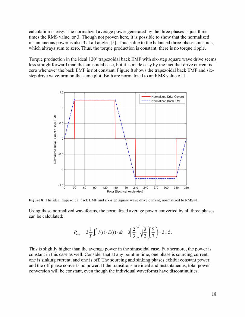
Torque production in the ideal 120º trapezoidal back EMF with six-step square wave drive seems less straightforward than the sinusoidal case, but it is made easy by the fact that drive current is zero whenever the back EMF is not constant. Figure 8 shows the trapezoidal back EMF and six-step drive waveform on the same plot. Both are normalized to an RMS value of 1.

0 30 60 90 120 150 180 210 240 270 300 330 360-1.5

-1

-0.5

0

0.5

1

1.5

Rotor Electrical Angle (deg)

Nor

mal

ized

Driv

e C

urre

nt /

Bac

k E

MF

Normalized Drive Current

Normalized Back EMF

Figure 8: The ideal trapezoidal back EMF and six-step square wave drive current, normalized to RMS=1.

Using these normalized waveforms, the normalized average power converted by all three phases can be calculated:

15.37

9

2

3

3

23)()(

13

0

dttEtI

TP

T

avg .

This is slightly higher than the average power in the sinusoidal case. Furthermore, the power is constant in this case as well. Consider that at any point in time, one phase is sourcing current, one is sinking current, and one is off. The sourcing and sinking phases exhibit constant power, and the off phase converts no power. If the transitions are ideal and instantaneous, total power conversion will be constant, even though the individual waveforms have discontinuities.

19

One question to ask is whether normalizing to the RMS values leads to a fair comparison of torque production. From the point of view of the drive current, this implies that a motor with a given phase resistance would generate the same amount of heat with either drive waveform. This seems like a good basis for comparison, since it represents a physical limitation of the motor and drive. Additionally, enforcing that the back EMF waveforms also be normalized by RMS value says something about the motor’s intrinsic power conversion capability. (Think of the heat it would generate if driven by an external source with the phases shorted.)

Six-step square wave drive into an ideal 120º trapezoidal back EMF appears to have a slight advantage over pure sinusoidal drive with sinusoidal back EMF based on this normalization. It can generate about 5% more torque per unit heat dissipation, and the torque production is theoretically ripple-free. Additionally, the lower peak back EMF means that the motor will be able to achieve a higher speed at a given DC bus (battery) voltage.

The disadvantages of square-wave commutation only become clear when motor inductance is included in the analysis. Consider the practical implications of motor inductance on the six-step square wave drive. Sharp transitions in current are no longer possible, so there will be a necessary rise and fall time for the drive current. Flyback diodes will enforce this rise and fall time, even during the “Off” states in the six-step commutation sequence. The exact effects of motor inductance and diode conduction in the brushless DC scenario depend on many factors and require simulation to accurately predict. In general, though, torque production will no longer be constant (there will be torque ripple), and extra heat will be dissipated in the controller diodes.

Sine wave commutation, on the other hand, handles motor inductance almost in-stride. A pure sine wave passed through any complex impedance is still a pure sine wave with the same frequency, although it can be shifted in phase and attenuated. Thus, the set of three-phase sinusoidal drive currents and back EMF waveforms maintain a balanced operating point with constant torque, even in the presence of inductance. Torque output may be reduced, since current will lag back EMF, but it will still be ripple-free. (Field-oriented control attempts to correct for this lag.) Additionally, there is no diode conduction, since there is no “Off” state; all three phases are always being driven.

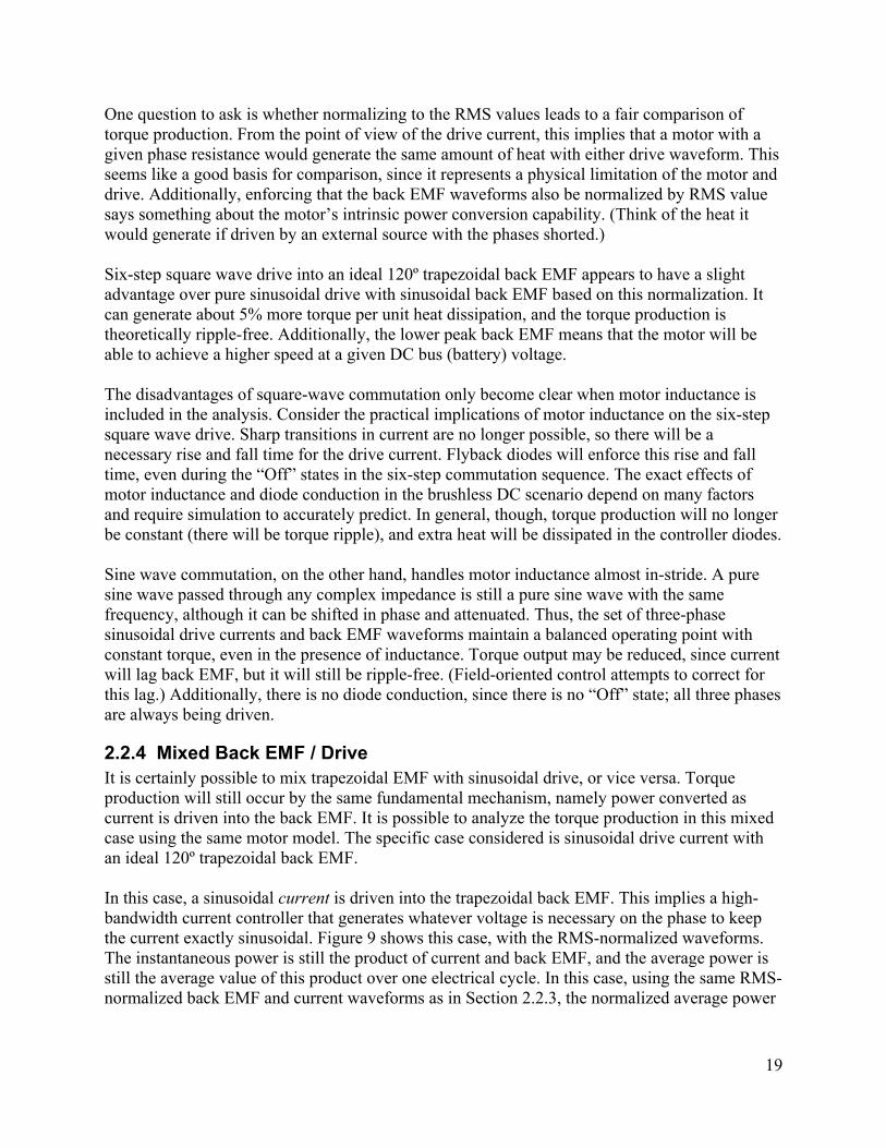
2.2.4 Mixed Back EMF / DriveIt is certainly possible to mix trapezoidal EMF with sinusoidal drive, or vice versa. Torque production will still occur by the same fundamental mechanism, namely power converted as current is driven into the back EMF. It is possible to analyze the torque production in this mixed case using the same motor model. The specific case considered is sinusoidal drive current with an ideal 120º trapezoidal back EMF.

In this case, a sinusoidal current is driven into the trapezoidal back EMF. This implies a high-bandwidth current controller that generates whatever voltage is necessary on the phase to keep the current exactly sinusoidal. Figure 9 shows this case, with the RMS-normalized waveforms. The instantaneous power is still the product of current and back EMF, and the average power is still the average value of this product over one electrical cycle. In this case, using the same RMS-normalized back EMF and current waveforms as in Section 2.2.3, the normalized average power

20

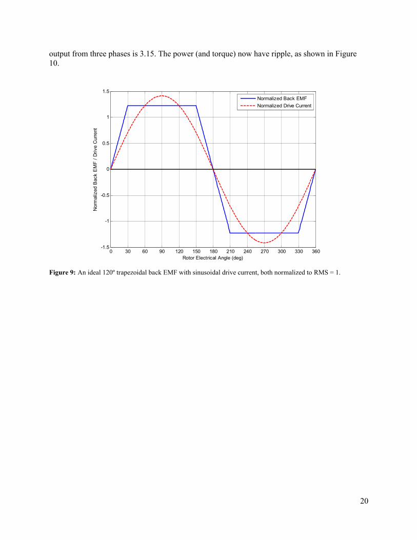
output from three phases is 3.15. The power (and torque) now have ripple, as shown in Figure 10.

0 30 60 90 120 150 180 210 240 270 300 330 360-1.5

-1

-0.5

0

0.5

1

1.5

Rotor Electrical Angle (deg)

Nor

mal

ized

Bac

k E

MF

/ D

rive

Cur

rent

Normalized Back EMF

Normalized Drive Current

Figure 9: An ideal 120º trapezoidal back EMF with sinusoidal drive current, both normalized to RMS = 1.

21

0 30 60 90 120 150 180 210 240 270 300 330 3600

0.5

1

1.5

2

2.5

3

3.5

4

Rotor Electrical Angle

Nor

mal

ized

Pow

er f

or T

hree

Pha

ses

Figure 10: The normalized power output of a sinusoidal drive current into an ideal 120º trapezoidal back EMF. The power and torque contain ripple at six times the electrical frequency.

One subtlety of this analysis is the assumption of sinusoidal drive current, not drive voltage. This requires a high-bandwidth current controller on each phase, which is possible but may not be the most practical solution. Simpler solutions that generate a sinusoidal drive voltage can also be implemented, as discussed in Section 4. The resulting drive current would no longer be a pure sinusoid, but the exact effect on torque ripple is not obvious due to the trapezoidal back EMF.

2.2.5 DC vs. AC SummaryAlthough the same physical principles apply to both, the definitions of brushless DC and synchronous AC motors are often confusing. Brushless DC (BLDC) is the term typically applied to motors with a more trapezoidal back EMF, driven by six-step square wave commutation. Synchronous AC, permanent magnet AC (PMAC), and permanent magnet synchronous motor (PMSM) are all terms typically applied to motors with sinusoidal back EMF being driven by sinusoidal currents. Thus, the definition depends both on the motor and on the drive. It is also possible to mix trapezoidal back EMF with sinusoidal drive, or sinusoidal back EMF with six-step commutation. The fundamental mechanism of torque production is the same, but the average and instantaneous power can differ slightly.

Table 2 summarizes the three cases explored in this section: pure BLDC, pure synchronous AC, and a mix of trapezoidal back EMF with sinusoidal drive current. The relative power (torque) production of each case is normalized to a physical constraint: heat dissipation in the motor. This is done by setting the RMS value of all the drive and back EMF waveforms equal to 1. This is not an exhaustive analysis, since there are any number of back EMF shapes that aren’t pure sinusoidal or trapezoidal, as well as other drive combinations. These three cases are also all

22

analyzed absent motor inductance, which can greatly change the story. A complete understanding of the relative performance of DC vs. AC drive for a given motor (specific back EMF, resistance, and inductance) would only be possible with simulation.

Table 2: A summary of the three combinations of back EMF and drive waveforms considered in this section, including the standard BLDC and PMSM/PMAC cases, plus a mixed case.

Normalized Power/ Torque (x3 Phases)

Power/TorqueRipple?

Comments

Sinusoidal Back EMFSinusoidal Drive

3.00 No PMSM / PMACNo ripple, even with inductance.

120º Trapezoidal Back EMFSix-Step Square Wave Drive

3.15 No* BLDC. *Ripple-free only in the ideal case with no inductance.

120º Trapezoidal Back EMFSinusoidal Drive

3.15 Yes, ~ 17%

The take-away from Table 2 might be that the difference between AC and DC is not as great as one might think. Under ideal conditions, both synchronous AC and brushless DC motors can produce nearly the same torque per unit heat dissipation, and with relatively little ripple. Brushless DC usually has a slight edge in torque production and achievable speed for a given voltage. However, AC drive with sinusoidal back EMF remains ripple-free even in the presence of inductance, while brushless DC does not (high frequency components of the drive current get filtered out). As the motor inductance and/or speed increase, the benefits of synchronous AC become greater. In the next section, field-oriented control of synchronous AC motors will be presented as a way to further accommodate for motor inductance in the sinusoidal case.

2.3 Field-Oriented ControlField-oriented control (FOC) is an advanced control technique used primarily for AC induction motors and permanent magnet synchronous motors. It has the advantage of isolating the torque-producing component of motor current from the field-augmenting or field-weakening component. This allows for a simple and independent torque controller and field controller, as would be the case with a separately-excited DC motor. Field-oriented control is not synonymous with space vector modulation (SVM), sinusoidal commutation, or phase advance, though all or some of these other techniques may be used to achieve field-oriented control.

This report will focus on field-oriented control as it applies to permanent magnet synchronous motors. In PMSM, it is very easy to isolates the torque-producing component of motor current by working in the rotating reference frame of the rotor, which is called the d-q reference frame. Motor quantities can be mapped into the d-q frame by simple trigonometry, and current (torque, field) control can be executed in this frame. This control method is called a synchronous current regulator. Though it is computationally intensive, one goal of this report is to highlight ways to do this efficiently on low-cost hardware. A modified synchronous current regulator optimized for computational efficiency is presented in Section 4.5.

2.3.1 d-q Reference FrameEssential to field-oriented control in PMSM is the establishment of a frame of reference that is fixed with respect to the rotor. Even simple BLDC controllers accomplish this, to some extent, by using Hall effect sensors or back EMF sensing to estimate rotor position. Field-oriented control goes a step further by using a finer rotor position estimate to map motor currents into the

23

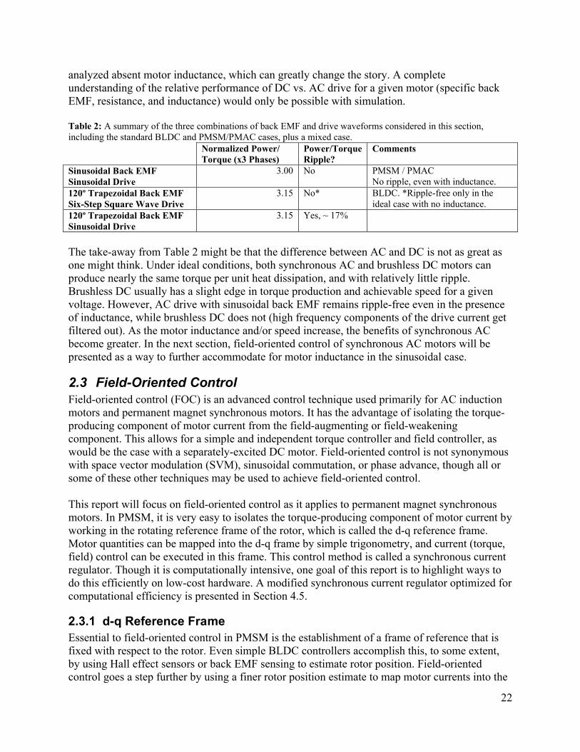
rotating frame. The rotating frame is defined by two axes, labeled direct (d) and quadrature (q) and fixed to the rotor as illustrated in Figure 11. (An outside rotor is used to facilitate the illustration.)

Figure 11: The d-q reference frame is fixed to the rotor such that the d-axis always falls on the magnetic axis and the q-axis always falls in between the magnetic axis, 90º ahead in the direction of rotation.

The direct (d) axis is defined to be on the magnetic axis passing through the center of a set of permanent magnets on the rotor. The quadrature (q) axis is defined to be 90º electrical ahead of the q-axis in the direction of rotation. In other words, the q-axis always falls exactly between two magnets. In the case of a two-pole motor, this is identical to 90º mechanical, and the axes are physically orthogonal. For higher pole counts, the axes are not physically orthogonal. For example, in a four-pole motor, they are separated by 45º mechanical. For simplicity, the two-pole, outside rotor illustration in Figure 11 will be used throughout this section. Since motor quantities will be projected based on electrical angle measurements, the number of poles does not affect the control strategy.

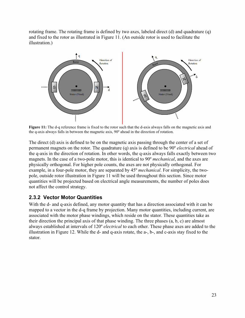
2.3.2 Vector Motor QuantitiesWith the d- and q-axis defined, any motor quantity that has a direction associated with it can be mapped to a vector in the d-q frame by projection. Many motor quantities, including current, are associated with the motor phase windings, which reside on the stator. These quantities take as their direction the principal axis of that phase winding. The three phases (a, b, c) are almostalways established at intervals of 120º electrical to each other. These phase axes are added to the illustration in Figure 12. While the d- and q-axis rotate, the a-, b-, and c-axis stay fixed to the stator.

24

Figure 12: The three phase winding of the motor defines three equally-spaced axes that are fixed to the stator, labeled a, b, and c.

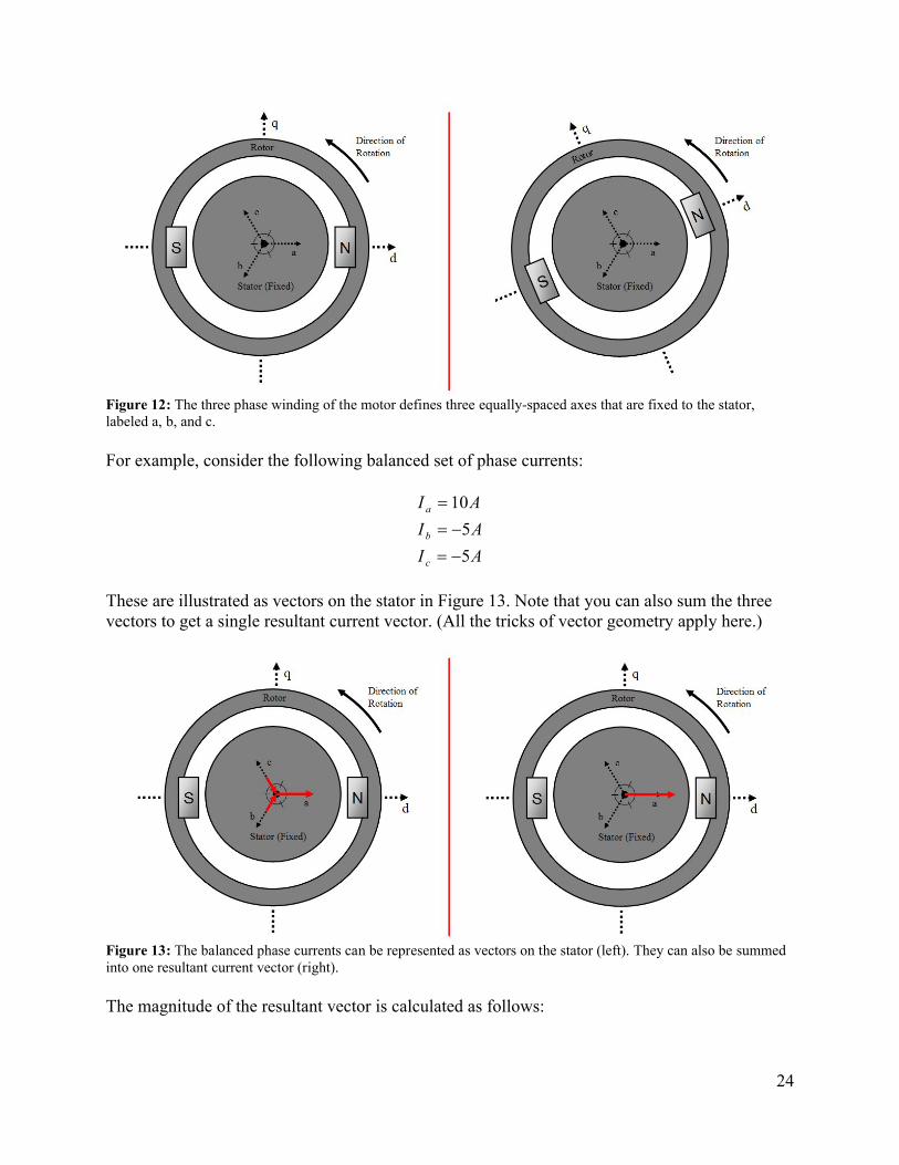
For example, consider the following balanced set of phase currents:

AI

AI

AI

c

b

a

5

5

10

These are illustrated as vectors on the stator in Figure 13. Note that you can also sum the three vectors to get a single resultant current vector. (All the tricks of vector geometry apply here.)

Figure 13: The balanced phase currents can be represented as vectors on the stator (left). They can also be summed into one resultant current vector (right).

The magnitude of the resultant vector is calculated as follows:

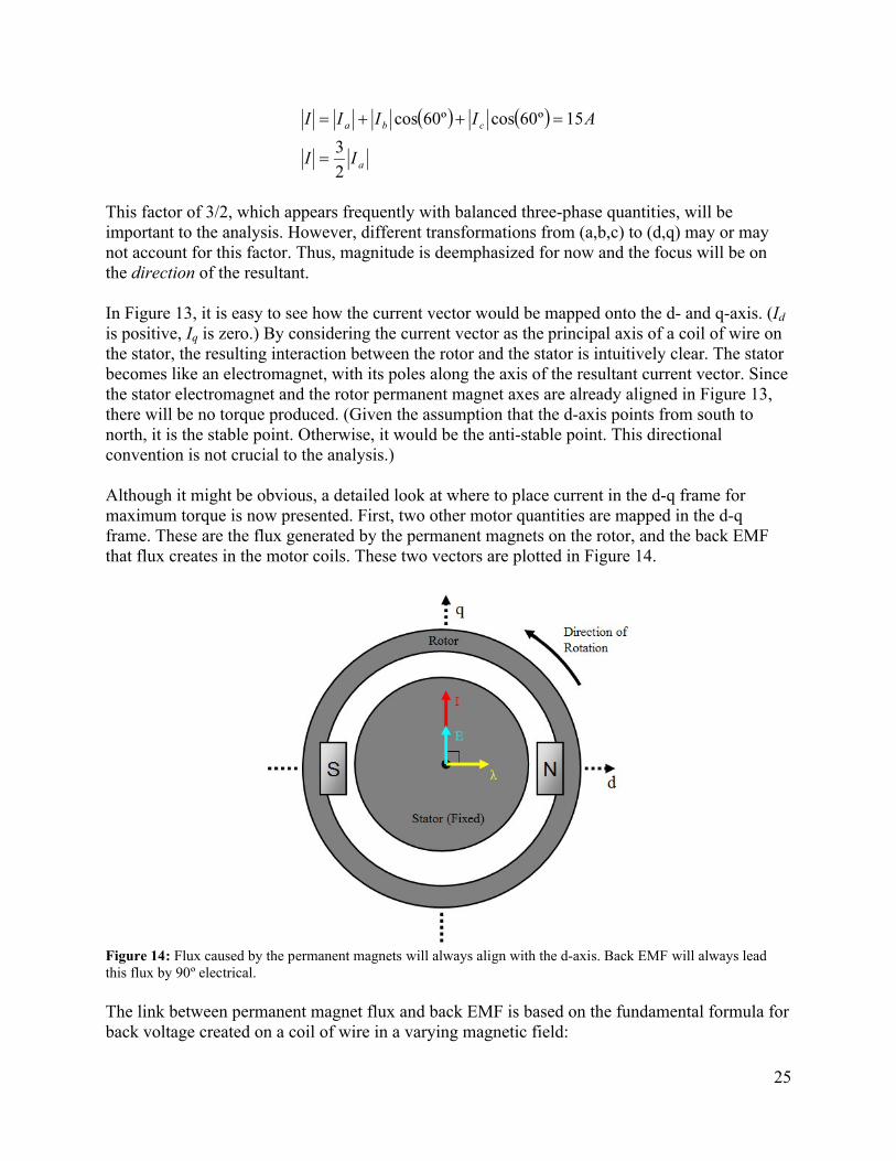
25

a

cba

II

AIIII

2

3

15º60cosº60cos

This factor of 3/2, which appears frequently with balanced three-phase quantities, will be important to the analysis. However, different transformations from (a,b,c) to (d,q) may or may not account for this factor. Thus, magnitude is deemphasized for now and the focus will be on the direction of the resultant.

In Figure 13, it is easy to see how the current vector would be mapped onto the d- and q-axis. (Id

is positive, Iq is zero.) By considering the current vector as the principal axis of a coil of wire on the stator, the resulting interaction between the rotor and the stator is intuitively clear. The stator becomes like an electromagnet, with its poles along the axis of the resultant current vector. Since the stator electromagnet and the rotor permanent magnet axes are already aligned in Figure 13, there will be no torque produced. (Given the assumption that the d-axis points from south to north, it is the stable point. Otherwise, it would be the anti-stable point. This directional convention is not crucial to the analysis.)

Although it might be obvious, a detailed look at where to place current in the d-q frame for maximum torque is now presented. First, two other motor quantities are mapped in the d-q frame. These are the flux generated by the permanent magnets on the rotor, and the back EMF that flux creates in the motor coils. These two vectors are plotted in Figure 14.

Figure 14: Flux caused by the permanent magnets will always align with the d-axis. Back EMF will always lead this flux by 90º electrical.

The link between permanent magnet flux and back EMF is based on the fundamental formula for back voltage created on a coil of wire in a varying magnetic field:

26

dt

dE

.

In the case of a sinusoidal time-varying flux, λ, the back EMF, E, will also be sinusoidal and will lead the flux by 90º. This is the condition illustrated in Figure 14, with the flux and back EMF vectors representing the instantaneous location of the peak flux and back EMF. These peaks will rotate with the d-q frame such that λ is always on the d-axis and E is always on the q-axis. Since the flux considered is from permanent magnets only, this is true regardless of stator current.

Given a rotor angular velocity, the magnitude of E is fixed by the motor constant. To convert as much power as possible with a given current, the dot product of the I and E vectors should be maximized. This occurs when current is on the q-axis exclusively. Maximizing power is the same as maximizing torque, since the speed is given. This analysis works as well in the limit as speed goes to zero. Thus, peak torque will always occur when current is on the q-axis.

2.3.3 Why Control is Necessary: Motor InductanceThe fundamental reason why field-oriented control is nontrivial stems from the nature of motor controllers themselves. Most often, they are created with elements that can be modeled as voltage sources. A set of two switching power devices creates a time-averaged voltage applied to each motor phase. This is an open-loop phenomenon: the voltage is exactly set by controlling the duty cycle of the two switching power devices.

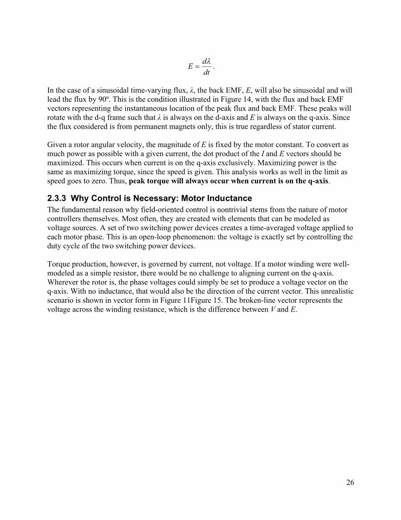
Torque production, however, is governed by current, not voltage. If a motor winding were well-modeled as a simple resistor, there would be no challenge to aligning current on the q-axis. Wherever the rotor is, the phase voltages could simply be set to produce a voltage vector on the q-axis. With no inductance, that would also be the direction of the current vector. This unrealistic scenario is shown in vector form in Figure 11Figure 15. The broken-line vector represents the voltage across the winding resistance, which is the difference between V and E.

27

Figure 15: This is what the essential motor quantities would look like in the absence of winding inductance. Voltage, current, and back EMF could all be easily aligned open-loop for maximum torque at any given rotor position.

A real motor, however, has some inductance. Inductors resist changes in current according to the constitutive equation:

.dt

dILVL

Thus some voltage will be developed across the winding inductance that resists changes in current. If an inductor is subjected to a sinusoidal time-varying voltage, the current will also be sinusoidal and will lag the voltage by 90º.

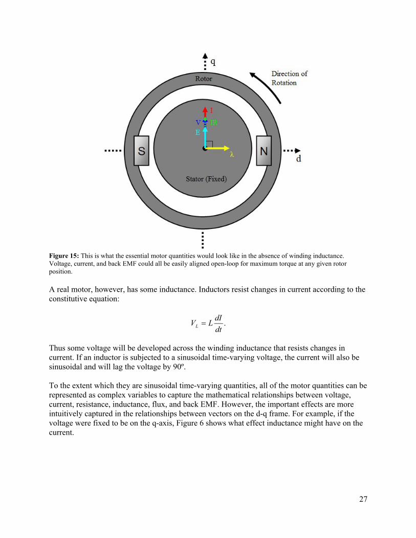
To the extent which they are sinusoidal time-varying quantities, all of the motor quantities can be represented as complex variables to capture the mathematical relationships between voltage, current, resistance, inductance, flux, and back EMF. However, the important effects are more intuitively captured in the relationships between vectors on the d-q frame. For example, if the voltage were fixed to be on the q-axis, Figure 6 shows what effect inductance might have on the current.

28

Figure 16: The vector relationships between motor quantities if the applied voltage is fixed to the q-axis, but there is inductance present.

Current now lags voltage, due to the inductance. The two broken-line vectors represent components of voltage across the winding resistance and winding inductance. The resistance component is parallel to current and the inductance component leads current by 90º. (In other words, current lags voltage across the inductor by 90º.) The vector sum of voltages is consistent with Kirchoff’s Voltage Law (KVL).

In Figure 16, current and back EMF are no longer aligned, so torque is not maximized. Open-loop phase advance is one possible way to accommodate for the affect of inductance: Simply placing voltage ahead of the q-axis by some angle (which could be a function of other motor parameters, measured or known) could offset most, if not all, of the angle lost to inductance. However, any solution based on open-loop phase advance would be motor-specific. Field-oriented control seeks a more flexible solution based on real-time current measurements.

2.3.4 Field-Oriented Control ObjectiveThe objective of field-oriented control is to achieve measurement and closed-loop control of the motor current vector, essentially placing it on the d-q plane. The controller presented is general enough to place the vector anywhere, including leading the q-axis to achieve field weakening. For the most part, though, this report will focus on placing the current vector on the q-axis, to optimize torque. Figure 17 shows the vector motor quantities might look like with the current vector controlled to be on the q-axis.

29

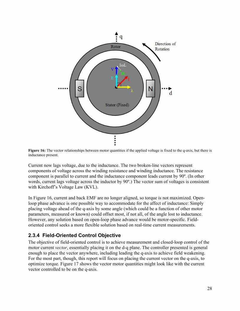
Figure 17: With current controlled to be on the q-axis, the voltage must lead the back EMF to account for inductance.

The voltage vector is advanced ahead of the back EMF. (In other words, Vd is negative.) This counteracts the lag introduced by motor inductance. Current still lags applied, but it is now in phase with back EMF, producing optimal torque. The broken-line vectors represent the components of voltage across the winding resistance and inductance needed to satisfy KVL. Here it is clear that if the product of current, speed, and inductance is sufficiently small as to be negligible, the degenerate case is that of Figure 15. This product (normalized to the applied voltage) can be used as a test for whether field-oriented control is justified for a given motor and operating range.

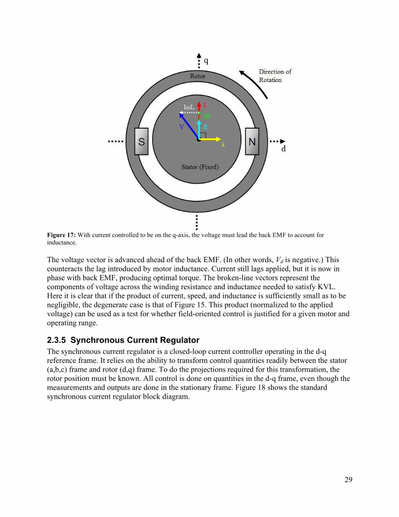
2.3.5 Synchronous Current RegulatorThe synchronous current regulator is a closed-loop current controller operating in the d-q reference frame. It relies on the ability to transform control quantities readily between the stator (a,b,c) frame and rotor (d,q) frame. To do the projections required for this transformation, the rotor position must be known. All control is done on quantities in the d-q frame, even though the measurements and outputs are done in the stationary frame. Figure 18 shows the standard synchronous current regulator block diagram.

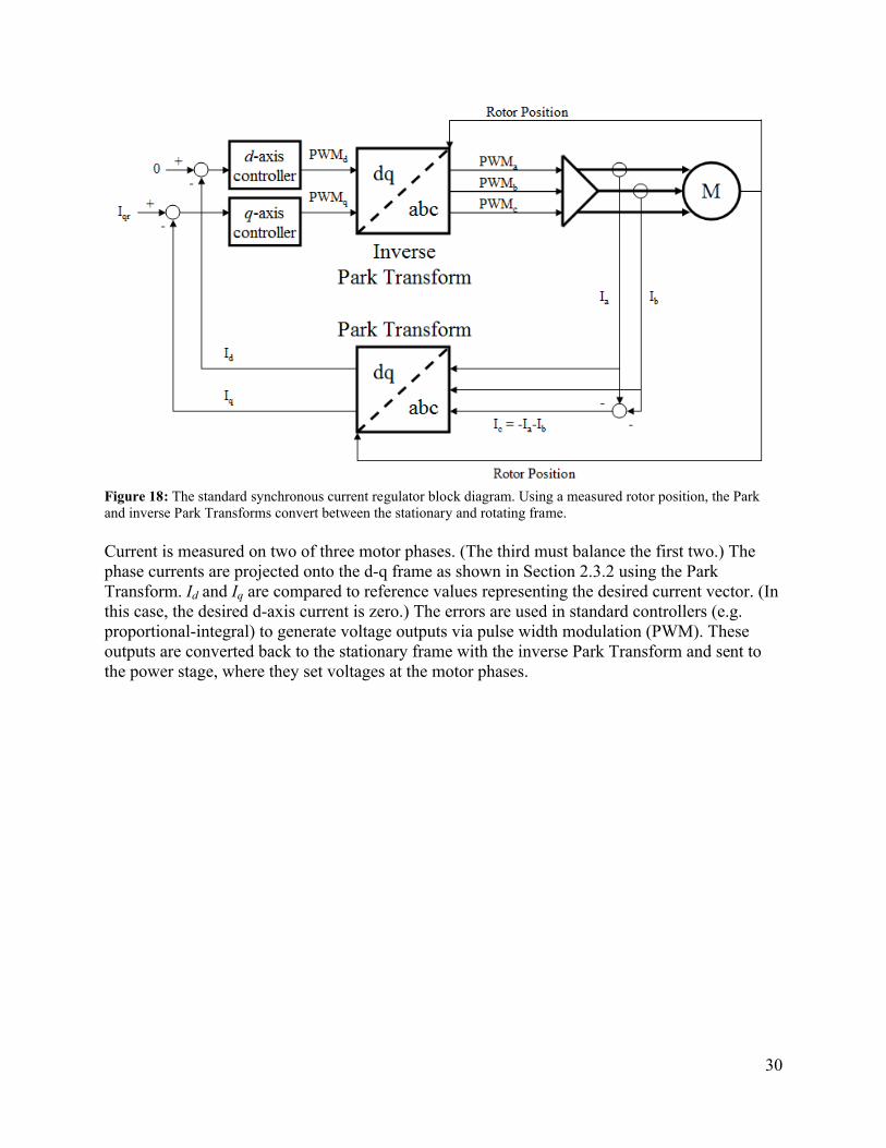
30

Figure 18: The standard synchronous current regulator block diagram. Using a measured rotor position, the Park and inverse Park Transforms convert between the stationary and rotating frame.

Current is measured on two of three motor phases. (The third must balance the first two.) The phase currents are projected onto the d-q frame as shown in Section 2.3.2 using the Park Transform. Id and Iq are compared to reference values representing the desired current vector. (In this case, the desired d-axis current is zero.) The errors are used in standard controllers (e.g. proportional-integral) to generate voltage outputs via pulse width modulation (PWM). These outputs are converted back to the stationary frame with the inverse Park Transform and sent to the power stage, where they set voltages at the motor phases.

31

3 Brushless Motor Design and Prototyping Methods

3.1 Design Strategy and GoalsThe ability to design motors to fit specific applications is an opportunity that is, in the opinion of the author, highly valuable and yet also not well-known. To most, the process of designing electric motor-based systems involves digging through catalogs of motors, immediately limiting the design space to a set of existing components. By the time this set is filtered by physical constraints and performance requirements, it may leave only a handful of options. Or, it may leave none. Breaking down the black-box status of electric motors to open up new design options is the primary goal of this study.

An important disclaimer: In most engineering situations, designing a custom motor is not called for. The set of commercially-available motors is actually fairly large, the pricing reasonable, and, most importantly, the design cycle time is shorter when components can be off-the-shelf. Only in specific instances where there is a gap in the set of available components is a custom design a viable option. The case study of direct-drive scooter motors is an example of this rare scenario. There is also a significant learning opportunity in designing a custom motor, which may have played an even larger role in the author’s motivation to pursue such projects. Learning the benefits and challenges of custom motor design by actually building motors is probably the best way to develop a feel for when such designs are a good option, and when off-the-shelf components will suffice.

Another goal of this study is to show that, by leveraging modern prototyping and analysis techniques and following simple design guidelines, the cost (in time and money) of designing a custom motor is greatly reduced. The above disclaimer notwithstanding, this may tip the balance in favor of a custom design in some instances. Analysis techniques which are useful include combined CAD/FEA using solid modeling and finite element magnetic simulation. This, with some first-order analysis, can give accurate motor performance predictions. CAM and rapid prototyping, using tools such as laser cutting and abrasive water jet machining, can make custom motor fabrication cost- and time-effective even in single quantities. Simple design guidelines that aid assembly (particularly for hand winding and magnet placement) can greatly speed up the process. Lastly, evaluation techniques that don’t require expensive equipment can quickly confirm motor performance. All of these techniques, applied at the “alpha prototype” phase, can help prove a motor design and secure resources for further development using more conventional analysis, tooling, and evaluation techniques.

In summary, the goals of this design study are to:1. Evaluate the conditions under which a custom motor design may be called for, and how

these conditions are affected by the availability of modern prototyping tools. Two case studies will be presented for which a custom motor design could be justified.

2. Demystify the design of custom brushless motors by showing simple analysis and simulation techniques as applied to the case studies.

3. Provide, though the case studies, some examples of modern rapid prototyping techniques for making custom motors.

32

4. Provide, through the case studies, good design practices that facilitate in-house motor assembly with no special tooling.

5. Evaluate whether the motors designed in the case studies meet requirements. If they do not, provide means to reconciling the measured performance with analysis and improve the design in future iterations.

3.2 Introduction of Case StudiesTwo case studies will be used in this section as real-life examples of custom motor design. The motors built for these two case studies are very different in scale and purpose. However, one goal of this section is to highlight some similarities in their design and prototyping methods. Wherever possible, the analytical methods will be applied to both cases to show the flexibility of motor analysis. Both motors also take advantage of rapid prototyping methods and design for assembly. Finally, the measured results are compared to analyses to evaluate the motors in each case and qualify the designs (with suggestions for future improvements).

3.2.1 Direct-Drive Kick Scooter MotorsThe first case study involves direct-drive electric scooter motors. For large, seated scooters and bicycles, there are a variety of commercial options for in-wheel motors. However, there are no commercially available in-wheel motors for small stand-on “kick scooters,” such as Razor scooters. A typical electric kick scooter might have a high-speed motor geared down by belt or chain to the rear wheel. Some benefits of an in-wheel motor include space efficiency, a minimum number of moving parts, no transmission losses, and a cleaner aesthetic more closely resembling an unpowered scooter. Some disadvantages include more complex control, coupling of an expensive component to one normally considered consumable, and exposure of the motor to vibration, dirt, and water.

Without the opportunity for gear reduction, the primary challenge of creating an in-wheel scooter motor is generating sufficient traction force in the direct-drive application. With no gear ratio to work with, and assuming a fixed ratio between the air gap and outer diameters, the force exerted by the wheel will scale linearly with motor current and length based on IL×B. Motor current, in turn, scales linearly with copper cross-sectional area. Roughly speaking, then, the force exerted will scale with the volume (length × area) of the in-wheel motor. So, a small wheel motor might need all the design help it can get to generate sufficient force to move a person.

The author cannot claim complete novelty of this design challenge. In fact, this project started with an inspirational proof of concept: a functional razor scooter-sized wheel motor built by Charles Guan ‘11, shown in Figure 19.

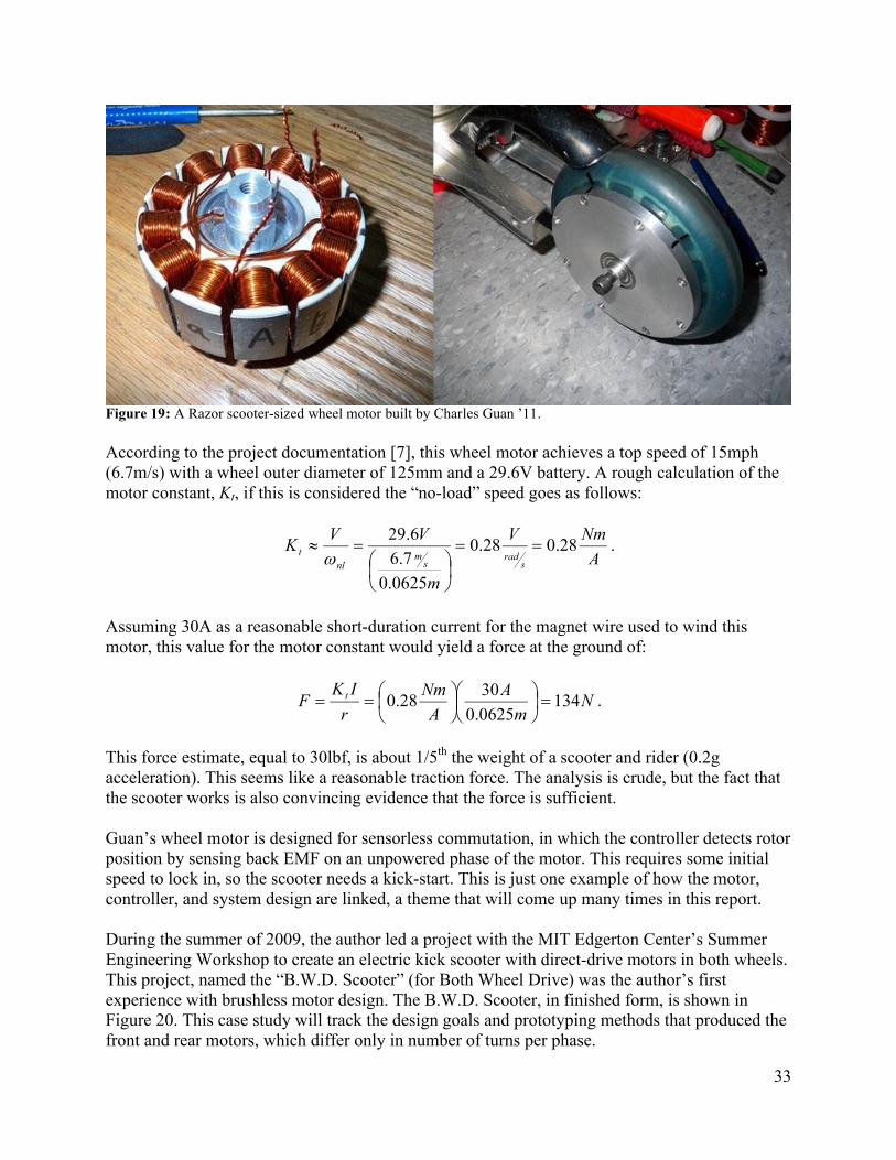
33

Figure 19: A Razor scooter-sized wheel motor built by Charles Guan ’11.

According to the project documentation [7], this wheel motor achieves a top speed of 15mph (6.7m/s) with a wheel outer diameter of 125mm and a 29.6V battery. A rough calculation of the motor constant, Kt, if this is considered the “no-load” speed goes as follows:

A

NmV

m

VVK

srad

sm

nlt 28.028.0

0625.0

7.6

6.29

.

Assuming 30A as a reasonable short-duration current for the magnet wire used to wind this motor, this value for the motor constant would yield a force at the ground of:

Nm

A

A

Nm

r

IKF t 134

0625.0

3028.0

.

This force estimate, equal to 30lbf, is about 1/5th the weight of a scooter and rider (0.2g acceleration). This seems like a reasonable traction force. The analysis is crude, but the fact that the scooter works is also convincing evidence that the force is sufficient.

Guan’s wheel motor is designed for sensorless commutation, in which the controller detects rotor position by sensing back EMF on an unpowered phase of the motor. This requires some initial speed to lock in, so the scooter needs a kick-start. This is just one example of how the motor, controller, and system design are linked, a theme that will come up many times in this report.

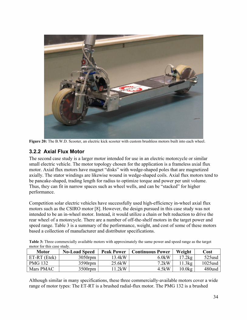
During the summer of 2009, the author led a project with the MIT Edgerton Center’s Summer Engineering Workshop to create an electric kick scooter with direct-drive motors in both wheels. This project, named the “B.W.D. Scooter” (for Both Wheel Drive) was the author’s first experience with brushless motor design. The B.W.D. Scooter, in finished form, is shown in Figure 20. This case study will track the design goals and prototyping methods that produced the front and rear motors, which differ only in number of turns per phase.

34

Figure 20: The B.W.D. Scooter, an electric kick scooter with custom brushless motors built into each wheel.

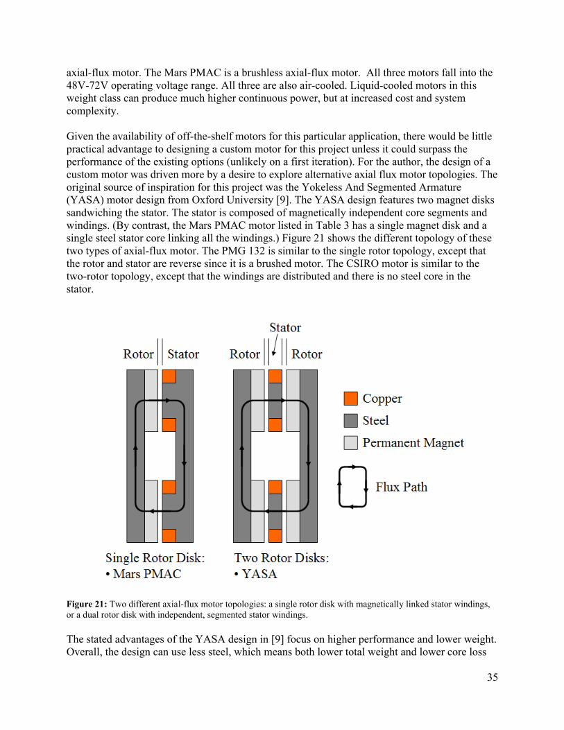
3.2.2 Axial Flux MotorThe second case study is a larger motor intended for use in an electric motorcycle or similar small electric vehicle. The motor topology chosen for the application is a frameless axial flux motor. Axial flux motors have magnet “disks” with wedge-shaped poles that are magnetized axially. The stator windings are likewise wound in wedge-shaped coils. Axial flux motors tend to be pancake-shaped, trading length for radius to optimize torque and power per unit volume. Thus, they can fit in narrow spaces such as wheel wells, and can be “stacked” for higher performance.

Competition solar electric vehicles have successfully used high-efficiency in-wheel axial flux motors such as the CSIRO motor [8]. However, the design pursued in this case study was not intended to be an in-wheel motor. Instead, it would utilize a chain or belt reduction to drive the rear wheel of a motorcycle. There are a number of off-the-shelf motors in the target power and speed range. Table 3 is a summary of the performance, weight, and cost of some of these motors based a collection of manufacturer and distributor specifications.

Table 3: Three commercially available motors with approximately the same power and speed range as the target motor for this case study.

Motor No-Load Speed Peak Power Continuous Power Weight CostET-RT (Etek) 3050rpm 13.4kW 6.0kW 17.2kg 525usdPMG 132 3590rpm 25.6kW 7.2kW 11.3kg 1025usdMars PMAC 3500rpm 11.2kW 4.5kW 10.0kg 480usd

Although similar in many specifications, these three commercially-available motors cover a wide range of motor types: The ET-RT is a brushed radial-flux motor. The PMG 132 is a brushed

35

axial-flux motor. The Mars PMAC is a brushless axial-flux motor. All three motors fall into the 48V-72V operating voltage range. All three are also air-cooled. Liquid-cooled motors in this weight class can produce much higher continuous power, but at increased cost and system complexity.

Given the availability of off-the-shelf motors for this particular application, there would be little practical advantage to designing a custom motor for this project unless it could surpass the performance of the existing options (unlikely on a first iteration). For the author, the design of a custom motor was driven more by a desire to explore alternative axial flux motor topologies. The original source of inspiration for this project was the Yokeless And Segmented Armature (YASA) motor design from Oxford University [9]. The YASA design features two magnet disks sandwiching the stator. The stator is composed of magnetically independent core segments and windings. (By contrast, the Mars PMAC motor listed in Table 3 has a single magnet disk and a single steel stator core linking all the windings.) Figure 21 shows the different topology of these two types of axial-flux motor. The PMG 132 is similar to the single rotor topology, except that the rotor and stator are reverse since it is a brushed motor. The CSIRO motor is similar to the two-rotor topology, except that the windings are distributed and there is no steel core in the stator.

Figure 21: Two different axial-flux motor topologies: a single rotor disk with magnetically linked stator windings, or a dual rotor disk with independent, segmented stator windings.

The stated advantages of the YASA design in [9] focus on higher performance and lower weight. Overall, the design can use less steel, which means both lower total weight and lower core loss

36

due to eddy currents in steel. Losses incurred in the extra rotor back-iron are small compared to what is saved by minimizing the stator core flux path, which is the part that sees high frequency alternating flux. Since the original paper, the YASA motor design has been scaled and commercialized for use in electrical vehicle drivetrains [10].

There are also many practical advantages of the segmented armature design not explicitly mentioned in the original paper. Most importantly for a project like this, it is easy to construct. The laminated stator segments are simple in geometry and can be built up and wound independently, by hand, before being assembled into the motor. This made it feasible to produce such a motor in-house with no special tooling.

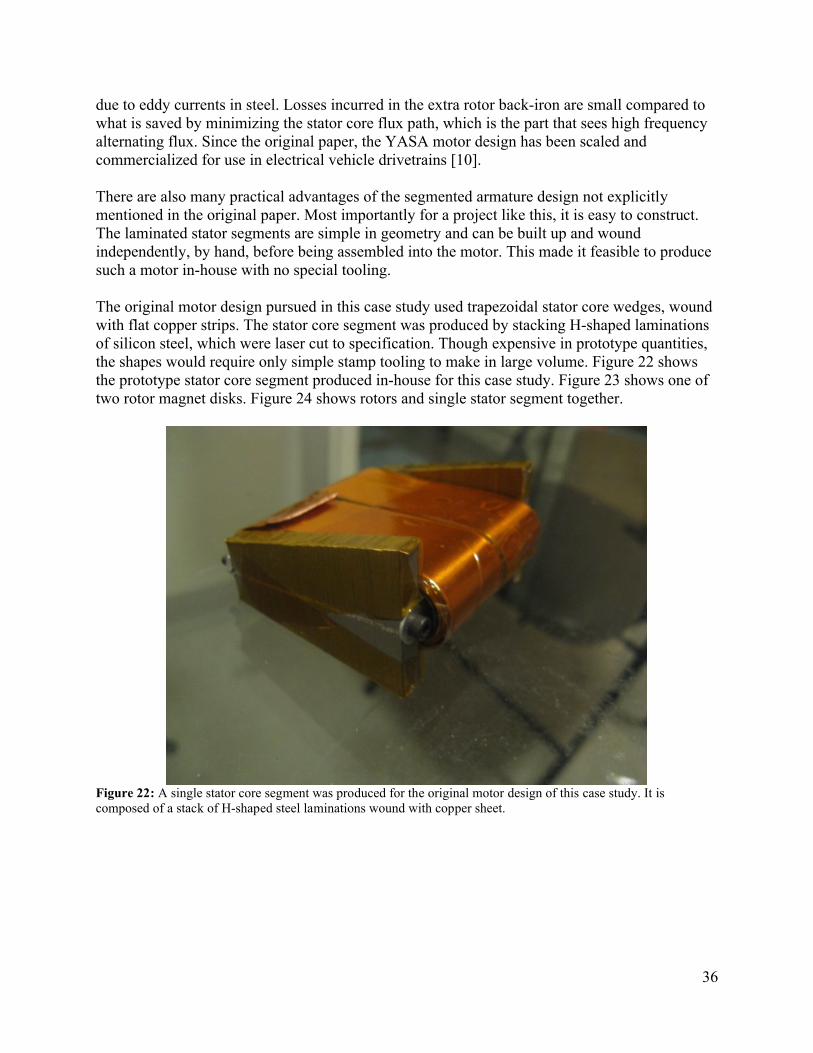
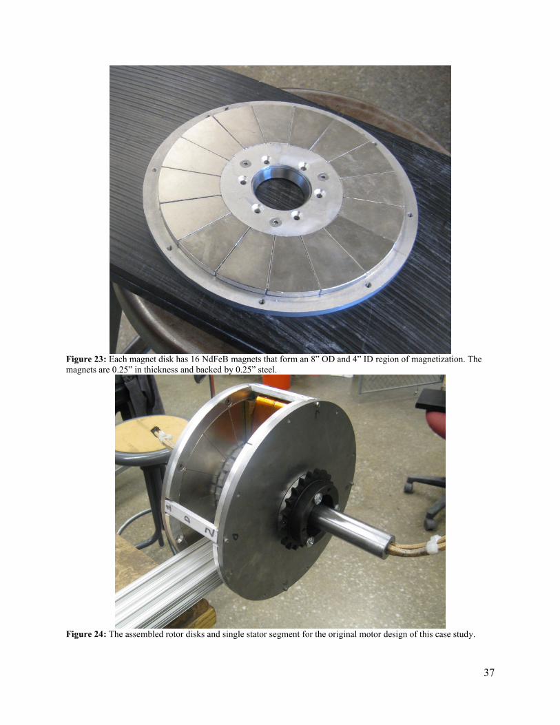
The original motor design pursued in this case study used trapezoidal stator core wedges, wound with flat copper strips. The stator core segment was produced by stacking H-shaped laminations of silicon steel, which were laser cut to specification. Though expensive in prototype quantities, the shapes would require only simple stamp tooling to make in large volume. Figure 22 shows the prototype stator core segment produced in-house for this case study. Figure 23 shows one of two rotor magnet disks. Figure 24 shows rotors and single stator segment together.

Figure 22: A single stator core segment was produced for the original motor design of this case study. It is composed of a stack of H-shaped steel laminations wound with copper sheet.

37

Figure 23: Each magnet disk has 16 NdFeB magnets that form an 8” OD and 4” ID region of magnetization. The magnets are 0.25” in thickness and backed by 0.25” steel.

Figure 24: The assembled rotor disks and single stator segment for the original motor design of this case study.

38

Despite the relative ease of fabrication and winding, several important challenges became clear during assembly and testing of this design. Perhaps the biggest mechanical challenge in designing an axial flux motor is the very large axial magnetic attraction force. In this particular motor design, the axial attraction forces could exceed 2,000N (500lbf) with all stator segments in place. Adequate thrust bearings turned out to be a necessary but not sufficient design consideration. The mechanical connection between rotor halves also contributes to the structural loop and was, in this case, inadequate to maintain a consistent air gap and bearing preload. A solid outer “can” would have been more appropriate, but difficult to machine in-house.

The technical challenges were not show-stoppers, but ultimately, the cost of producing a full set of stator core segments was not justifiable for this project. Since the motor seemed unlikely to fit the requirements of the vehicle for which it was originally being designed (a racing motorcycle), the primary focus shifted to a design study of this motor topology. While it wasn’t quite “back to the drawing board,” a step back to look at the big picture was called for.

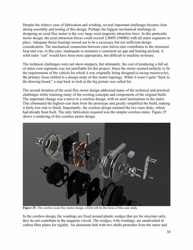
The second iteration of the axial flux motor design addressed many of the technical and practical challenges while retaining many of the existing concepts and components of the original build. The important change was a move to a coreless design, with no steel laminations in the stator. This eliminated the highest-cost item from the prototype and greatly simplified the build, making it fairly low-risk to finish. Importantly, the coreless design retained the two rotor disks, which had already been built. The only fabrication required was the simpler coreless stator. Figure 25shows a rendering of this coreless motor design.

Figure 25: The coreless axial flux motor design, which will be the focus of this case study.

In the coreless design, the windings are fixed around plastic wedges that are for structure only; they do not contribute to the magnetic circuit. The wedges, with windings, are sandwiched in carbon fiber plates for rigidity. An aluminum hub with two shafts protrudes from the stator and

39

the existing rotor disks ride on these shafts. Figure 26 shows the motor prototype which was built as part of this case study. The following are some key characteristics of the coreless design which address specific problems in the original design:

No stator segment laminations. This eliminates a high-cost, high-risk item from a prototype that no longer seemed to require the power of the original design.

No axial magnetic force between the rotor and stator (at no load). The lack of stator laminations and the use of stainless steel hardware eliminate any static magnetic attraction between the rotor and stator. A large axial attraction force still exists between the two rotor disks, but this force does not directly influence the stator, allowing for the construction of a thin, lightweight stator and making assembly significantly easier. (At least one disk will go on with no force.)

No cogging torque and direct magnetic coupling between rotor disks. With no steel stator segments, there is no cogging torque due to rotor-stator attraction. This results in very smooth low-speed operation. Strong magnetic coupling transmits torque directly between the two rotor disks. In fact, if only one side of the rotor is loaded, the other side will “follow,” keeping magnets in alignment without any mechanical coupling. Even if both sides are loaded, the differential torque required to slip a pole is very large.

Fully- and independently-constrained rotor halves. With no mechanical coupling between rotor halves, each was given both a radial and a thrust bearing to fully constrain it on the stator shaft. This made assembly and air gap maintenance much more straightforward.

More flexibility for mounting and wire entry. Wires enter from the side of the motor. A mounting flange for the stator also extends from one side. Air can also be blown directly through the side of the motor. These were all possibilities afforded by using independent rotor disks.

Additionally, the motor retains the practical benefits of the YASA design, namely ease of construction of the stator windings off-board. They are wound separately, then assembled into the completed stator. With magnetically-independent stator segments, simulation and testing were also simplified, as will be discussed in Section 3.6.1.

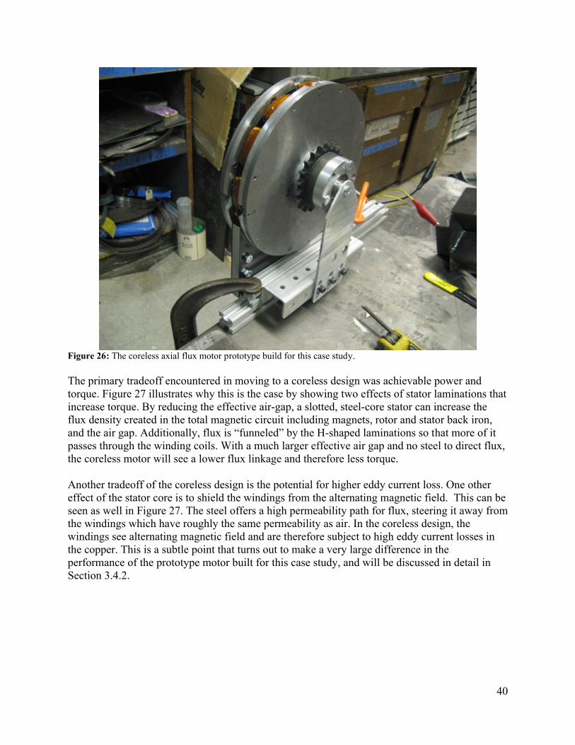
40

Figure 26: The coreless axial flux motor prototype build for this case study.

The primary tradeoff encountered in moving to a coreless design was achievable power and torque. Figure 27 illustrates why this is the case by showing two effects of stator laminations that increase torque. By reducing the effective air-gap, a slotted, steel-core stator can increase the flux density created in the total magnetic circuit including magnets, rotor and stator back iron, and the air gap. Additionally, flux is “funneled” by the H-shaped laminations so that more of it passes through the winding coils. With a much larger effective air gap and no steel to direct flux, the coreless motor will see a lower flux linkage and therefore less torque.

Another tradeoff of the coreless design is the potential for higher eddy current loss. One other effect of the stator core is to shield the windings from the alternating magnetic field. This can be seen as well in Figure 27. The steel offers a high permeability path for flux, steering it away from the windings which have roughly the same permeability as air. In the coreless design, the windings see alternating magnetic field and are therefore subject to high eddy current losses in the copper. This is a subtle point that turns out to make a very large difference in the performance of the prototype motor built for this case study, and will be discussed in detail in Section 3.4.2.

41

Figure 27: The slotted stator core creates a smaller effective air gap and directs more flux through the windings than the coreless design, giving it the potential to generate more torque.

Coreless motors can still have high torque/power density (due to weight savings). However, the decision to keep the existing rotor disks meant that this motor would sacrifice a lot of torque with only a modest reduction in weight. Future design iterations might benefit most from reduction of rotor mass and inertia by using a Halbach array of magnets which would not require steel backing.

The rest of this section will use the coreless version of the axial flux motor design as a case study, though much of the same analysis could also be applied to the original, slotted version.

3.3 Motor Constant: Various Prediction MethodsThe motor constant, along with resistance and inductance, are the three most important specifications of a permanent magnet motor (probably in that order). It is a measure of the torque production of the motor per unit amp. Via power conservation, the same constant is also a measure of the back EMF produced by the motor per unit speed. Section 2.1.2 introduced the motor model, back EMF, and motor constant, and showed how these concepts all relate. This section presents four ways to estimate the motor constant analytically and with the aid of simulation. The methods increase in complexity, but also in accuracy. Each method will be applied to the case study motors.

3.3.1 First-Order Analysis: DCThe first method of estimating the motor constant is static DC analysis using the Lorentz force on a wire. It is the simplest method, requiring only high-school physics, and works very well for back-of-the-envelope feasibility estimates. For example, this was the method used to evaluate the feasibility of the direct-drive kick-scooter motors.Figure 28a shows a single length of wire in a uniform magnetic field. The force, F, acting on the wire can be found by:

BLIF

,

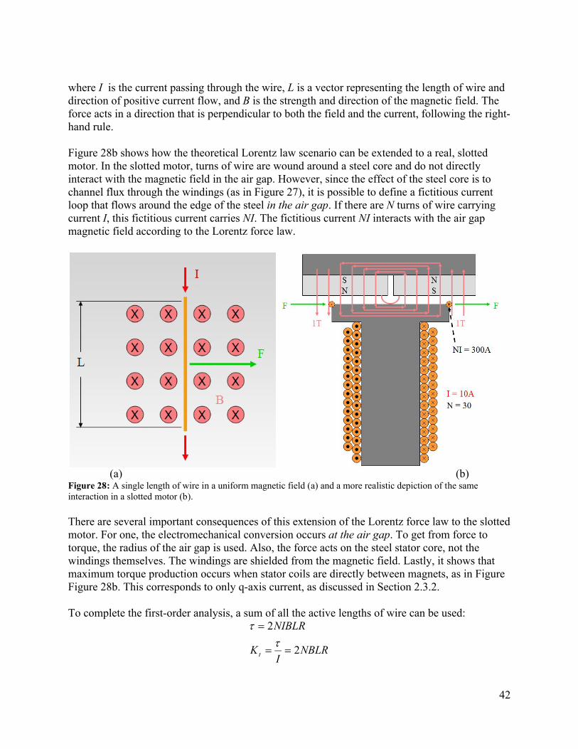
42

where I is the current passing through the wire, L is a vector representing the length of wire and direction of positive current flow, and B is the strength and direction of the magnetic field. The force acts in a direction that is perpendicular to both the field and the current, following the right-hand rule.

Figure 28b shows how the theoretical Lorentz law scenario can be extended to a real, slotted motor. In the slotted motor, turns of wire are wound around a steel core and do not directly interact with the magnetic field in the air gap. However, since the effect of the steel core is to channel flux through the windings (as in Figure 27), it is possible to define a fictitious current loop that flows around the edge of the steel in the air gap. If there are N turns of wire carrying current I, this fictitious current carries NI. The fictitious current NI interacts with the air gap magnetic field according to the Lorentz force law.

(a) (b)Figure 28: A single length of wire in a uniform magnetic field (a) and a more realistic depiction of the same interaction in a slotted motor (b).

There are several important consequences of this extension of the Lorentz force law to the slotted motor. For one, the electromechanical conversion occurs at the air gap. To get from force to torque, the radius of the air gap is used. Also, the force acts on the steel stator core, not the windings themselves. The windings are shielded from the magnetic field. Lastly, it shows that maximum torque production occurs when stator coils are directly between magnets, as in Figure Figure 28b. This corresponds to only q-axis current, as discussed in Section 2.3.2.

To complete the first-order analysis, a sum of all the active lengths of wire can be used:

NBLRI

K

NIBLR

t 2

2

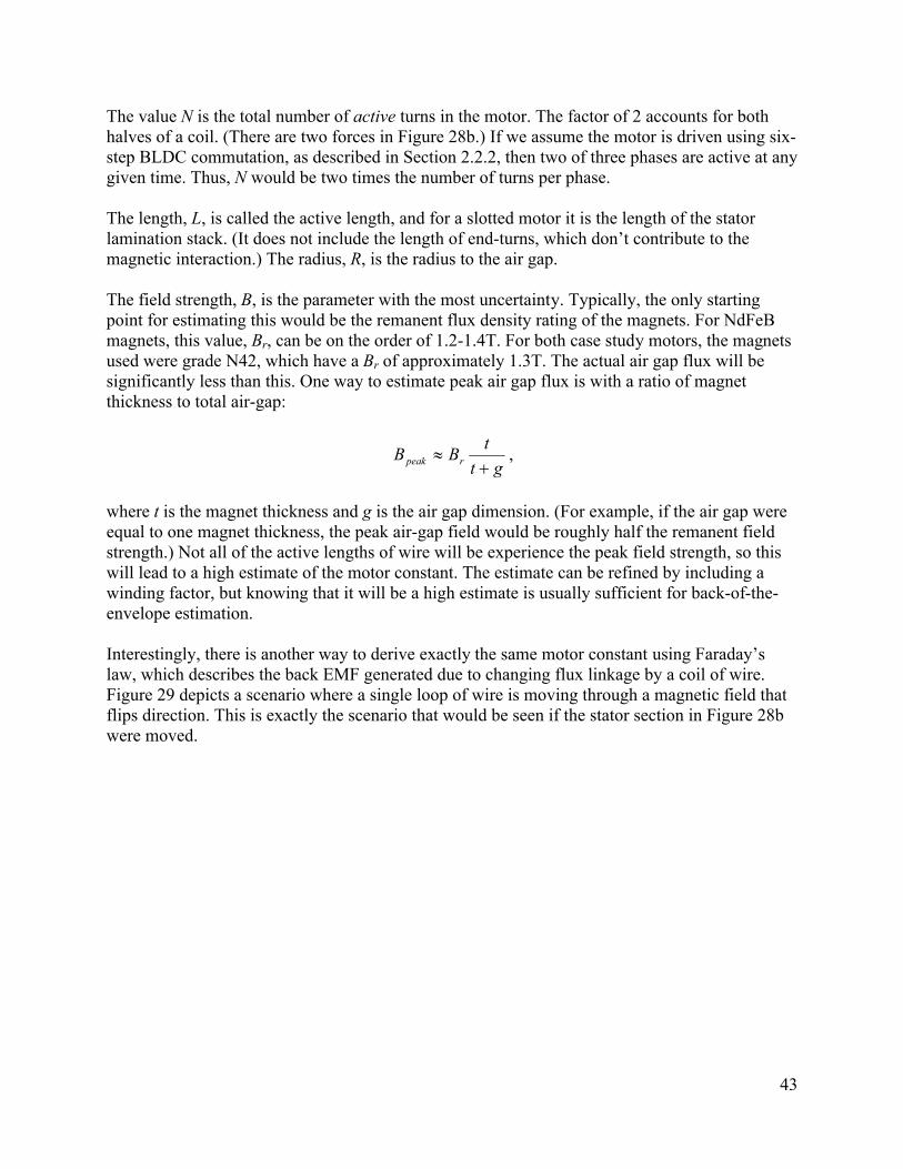
43

The value N is the total number of active turns in the motor. The factor of 2 accounts for both halves of a coil. (There are two forces in Figure 28b.) If we assume the motor is driven using six-step BLDC commutation, as described in Section 2.2.2, then two of three phases are active at any given time. Thus, N would be two times the number of turns per phase.

The length, L, is called the active length, and for a slotted motor it is the length of the stator lamination stack. (It does not include the length of end-turns, which don’t contribute to the magnetic interaction.) The radius, R, is the radius to the air gap.

The field strength, B, is the parameter with the most uncertainty. Typically, the only starting point for estimating this would be the remanent flux density rating of the magnets. For NdFeB magnets, this value, Br, can be on the order of 1.2-1.4T. For both case study motors, the magnets used were grade N42, which have a Br of approximately 1.3T. The actual air gap flux will be significantly less than this. One way to estimate peak air gap flux is with a ratio of magnet thickness to total air-gap:

gt

tBB rpeak

,

where t is the magnet thickness and g is the air gap dimension. (For example, if the air gap were equal to one magnet thickness, the peak air-gap field would be roughly half the remanent field strength.) Not all of the active lengths of wire will be experience the peak field strength, so this will lead to a high estimate of the motor constant. The estimate can be refined by including a winding factor, but knowing that it will be a high estimate is usually sufficient for back-of-the-envelope estimation.

Interestingly, there is another way to derive exactly the same motor constant using Faraday’s law, which describes the back EMF generated due to changing flux linkage by a coil of wire. Figure 29 depicts a scenario where a single loop of wire is moving through a magnetic field that flips direction. This is exactly the scenario that would be seen if the stator section in Figure 28b were moved.

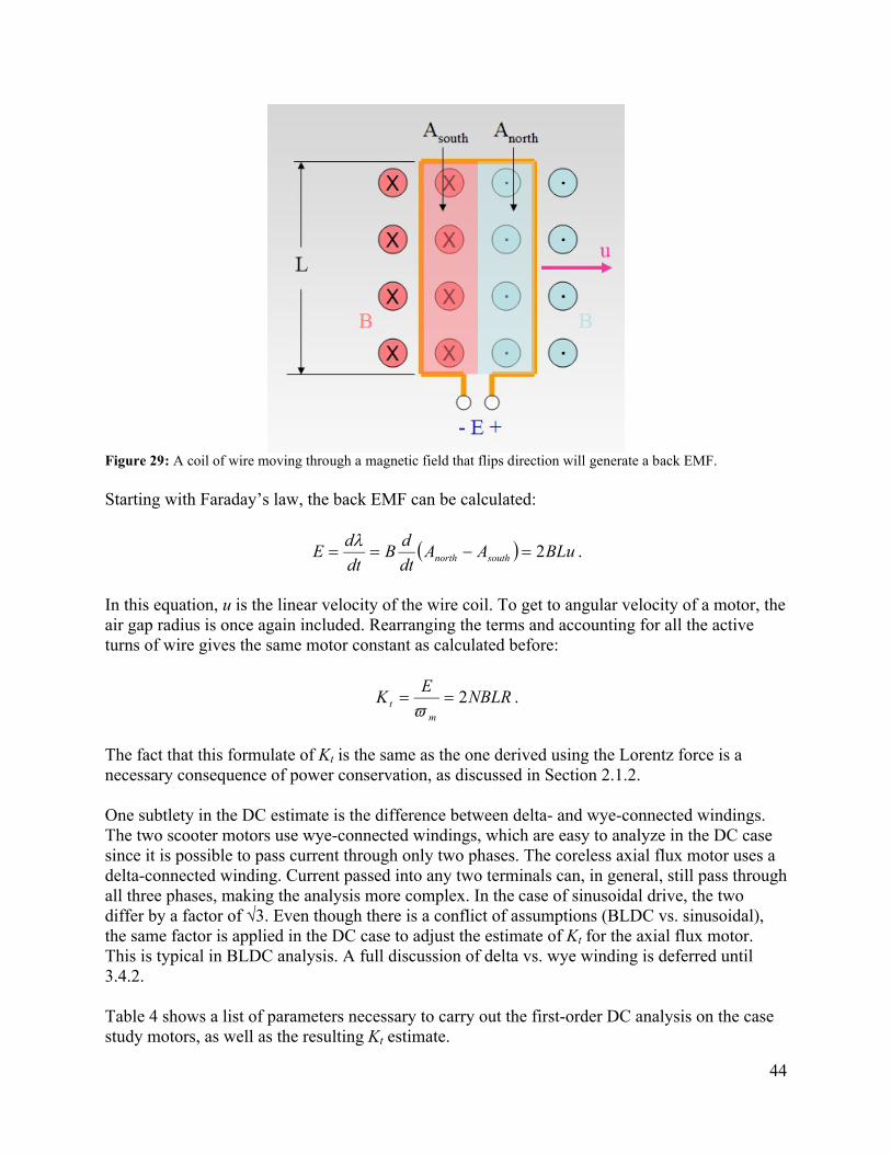
44

Figure 29: A coil of wire moving through a magnetic field that flips direction will generate a back EMF.

Starting with Faraday’s law, the back EMF can be calculated:

BLuAAdt

dB

dt

dE southnorth 2

.

In this equation, u is the linear velocity of the wire coil. To get to angular velocity of a motor, the air gap radius is once again included. Rearranging the terms and accounting for all the active turns of wire gives the same motor constant as calculated before:

NBLRE

Km

t 2

.

The fact that this formulate of Kt is the same as the one derived using the Lorentz force is a necessary consequence of power conservation, as discussed in Section 2.1.2.

One subtlety in the DC estimate is the difference between delta- and wye-connected windings. The two scooter motors use wye-connected windings, which are easy to analyze in the DC case since it is possible to pass current through only two phases. The coreless axial flux motor uses a delta-connected winding. Current passed into any two terminals can, in general, still pass through all three phases, making the analysis more complex. In the case of sinusoidal drive, the two differ by a factor of √3. Even though there is a conflict of assumptions (BLDC vs. sinusoidal), the same factor is applied in the DC case to adjust the estimate of Kt for the axial flux motor. This is typical in BLDC analysis. A full discussion of delta vs. wye winding is deferred until 3.4.2.

Table 4 shows a list of parameters necessary to carry out the first-order DC analysis on the case study motors, as well as the resulting Kt estimate.

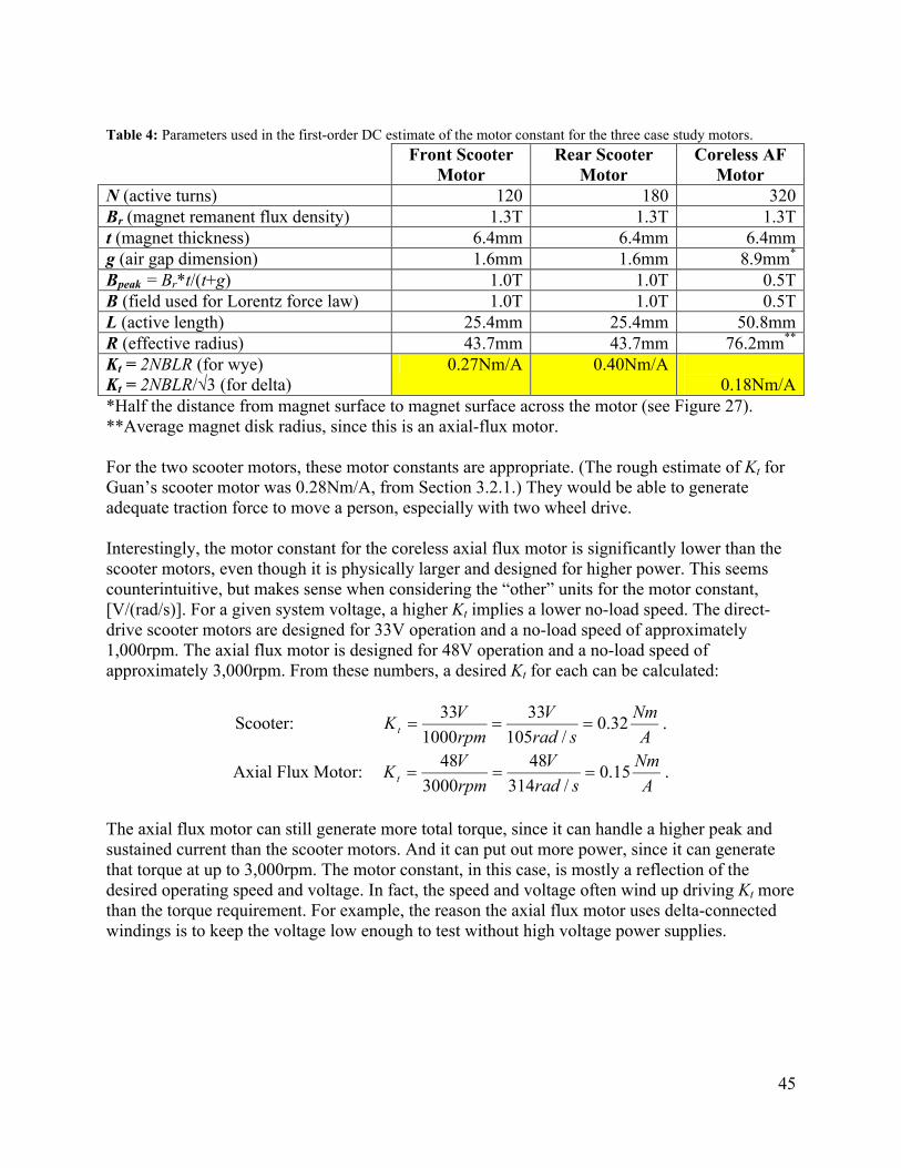
45

Table 4: Parameters used in the first-order DC estimate of the motor constant for the three case study motors.

Front Scooter Motor

Rear Scooter Motor

Coreless AF Motor

N (active turns) 120 180 320Br (magnet remanent flux density) 1.3T 1.3T 1.3Tt (magnet thickness) 6.4mm 6.4mm 6.4mmg (air gap dimension) 1.6mm 1.6mm 8.9mm*

Bpeak = Br*t/(t+g) 1.0T 1.0T 0.5TB (field used for Lorentz force law) 1.0T 1.0T 0.5TL (active length) 25.4mm 25.4mm 50.8mmR (effective radius) 43.7mm 43.7mm 76.2mm**

Kt = 2NBLR (for wye)Kt = 2NBLR/√3 (for delta)

0.27Nm/A 0.40Nm/A0.18Nm/A

*Half the distance from magnet surface to magnet surface across the motor (see Figure 27).**Average magnet disk radius, since this is an axial-flux motor.

For the two scooter motors, these motor constants are appropriate. (The rough estimate of Kt for Guan’s scooter motor was 0.28Nm/A, from Section 3.2.1.) They would be able to generate adequate traction force to move a person, especially with two wheel drive.

Interestingly, the motor constant for the coreless axial flux motor is significantly lower than the scooter motors, even though it is physically larger and designed for higher power. This seems counterintuitive, but makes sense when considering the “other” units for the motor constant, [V/(rad/s)]. For a given system voltage, a higher Kt implies a lower no-load speed. The direct-drive scooter motors are designed for 33V operation and a no-load speed of approximately 1,000rpm. The axial flux motor is designed for 48V operation and a no-load speed of approximately 3,000rpm. From these numbers, a desired Kt for each can be calculated:

Scooter: A

Nm

srad

V

rpm

VKt 32.0

/105

33

1000

33 .

Axial Flux Motor: A

Nm

srad

V

rpm

VKt 15.0

/314

48

3000

48 .

The axial flux motor can still generate more total torque, since it can handle a higher peak and sustained current than the scooter motors. And it can put out more power, since it can generate that torque at up to 3,000rpm. The motor constant, in this case, is mostly a reflection of the desired operating speed and voltage. In fact, the speed and voltage often wind up driving Kt more than the torque requirement. For example, the reason the axial flux motor uses delta-connected windings is to keep the voltage low enough to test without high voltage power supplies.

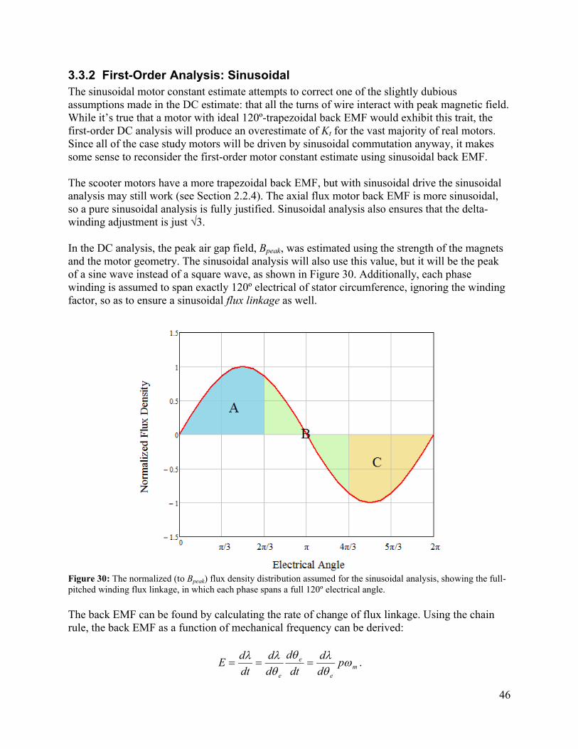
46

3.3.2 First-Order Analysis: SinusoidalThe sinusoidal motor constant estimate attempts to correct one of the slightly dubious assumptions made in the DC estimate: that all the turns of wire interact with peak magnetic field. While it’s true that a motor with ideal 120º-trapezoidal back EMF would exhibit this trait, the first-order DC analysis will produce an overestimate of Kt for the vast majority of real motors. Since all of the case study motors will be driven by sinusoidal commutation anyway, it makes some sense to reconsider the first-order motor constant estimate using sinusoidal back EMF.

The scooter motors have a more trapezoidal back EMF, but with sinusoidal drive the sinusoidal analysis may still work (see Section 2.2.4). The axial flux motor back EMF is more sinusoidal, so a pure sinusoidal analysis is fully justified. Sinusoidal analysis also ensures that the delta-winding adjustment is just √3.

In the DC analysis, the peak air gap field, Bpeak, was estimated using the strength of the magnets and the motor geometry. The sinusoidal analysis will also use this value, but it will be the peak of a sine wave instead of a square wave, as shown in Figure 30. Additionally, each phase winding is assumed to span exactly 120º electrical of stator circumference, ignoring the winding factor, so as to ensure a sinusoidal flux linkage as well.

Figure 30: The normalized (to Bpeak) flux density distribution assumed for the sinusoidal analysis, showing the full-pitched winding flux linkage, in which each phase spans a full 120º electrical angle.

The back EMF can be found by calculating the rate of change of flux linkage. Using the chain rule, the back EMF as a function of mechanical frequency can be derived:

me

e

e

pd

d

dt

d

d

d

dt

dE

.

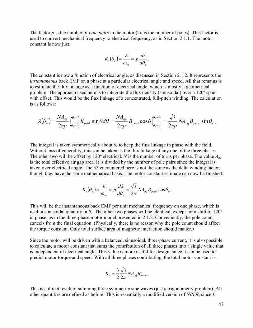
47

The factor p is the number of pole pairs in the motor (2p is the number of poles). This factor is used to convert mechanical frequency to electrical frequency, as in Section 2.1.1. The motor constant is now just:

em

et d

dp

EK

.

The constant is now a function of electrical angle, as discussed in Section 2.1.2. It represents the instantaneous back EMF on a phase at a particular electrical angle and speed. All that remains is to estimate the flux linkage as a function of electrical angle, which is mostly a geometrical problem. The approach used here is to integrate the flux density (sinusoidal) over a 120º span, with offset. This would be the flux linkage of a concentrated, full-pitch winding. The calculation is as follows:

epeakagpeakag

peakag

e BNAp

Bp

NAdB

p

NA e

e

e

e

sin

2

3cos

2sin

23

3

3

3

.

The integral is taken symmetrically about θe to keep the flux linkage in phase with the field. Without loss of generality, this can be taken as the flux linkage of any one of the three phases. The other two will be offset by 120º electrical. N is the number of turns per phase. The value Aag

is the total effective air gap area. It is divided by the number of pole pairs since the integral is taken over electrical angle. The √3 encountered here is not the same as the delta winding factor, though they have the same mathematical basis. The motor constant estimate can now be finished:

epeakagem

et BNAd

dp

EK

cos

2

3 .

This will be the instantaneous back EMF per unit mechanical frequency on one phase, which is itself a sinusoidal quantity in θe. The other two phases will be identical, except for a shift of 120º in phase, as in the three-phase motor model presented in 2.1.2. Conveniently, the pole count cancels from the final equation. (Physically, there is no reason why the pole count should affect the torque constant. Only total surface area of magnetic interaction should matter.)

Since the motor will be driven with a balanced, sinusoidal, three-phase current, it is also possible to calculate a motor constant that sums the contribution of all three phases into a single value that is independent of electrical angle. This value is more useful for design, since it can be used to predict motor torque and speed. With all three phases contributing, the total motor constant is:

peakagt BNAK2

3

2

3 .

This is a direct result of summing three symmetric sine waves (just a trigonometry problem). All other quantities are defined as before. This is essentially a modified version of NBLR, since L

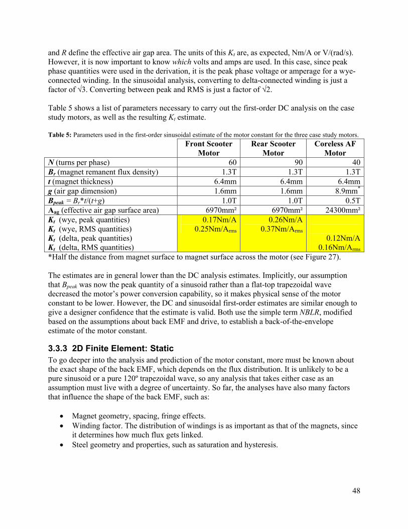
48

and R define the effective air gap area. The units of this Kt are, as expected, Nm/A or V/(rad/s). However, it is now important to know which volts and amps are used. In this case, since peak phase quantities were used in the derivation, it is the peak phase voltage or amperage for a wye-connected winding. In the sinusoidal analysis, converting to delta-connected winding is just a factor of √3. Converting between peak and RMS is just a factor of √2.

Table 5 shows a list of parameters necessary to carry out the first-order DC analysis on the case study motors, as well as the resulting Kt estimate.

Table 5: Parameters used in the first-order sinusoidal estimate of the motor constant for the three case study motors.

Front Scooter Motor

Rear Scooter Motor

Coreless AF Motor

N (turns per phase) 60 90 40Br (magnet remanent flux density) 1.3T 1.3T 1.3Tt (magnet thickness) 6.4mm 6.4mm 6.4mmg (air gap dimension) 1.6mm 1.6mm 8.9mm*

Bpeak = Br*t/(t+g) 1.0T 1.0T 0.5TAag (effective air gap surface area) 6970mm² 6970mm² 24300mm²Kt (wye, peak quantities)Kt (wye, RMS quantities)Kt (delta, peak quantities)Kt (delta, RMS quantities)

0.17Nm/A 0.25Nm/Arms

0.26Nm/A0.37Nm/Arms

0.12Nm/A0.16Nm/Arms

*Half the distance from magnet surface to magnet surface across the motor (see Figure 27).

The estimates are in general lower than the DC analysis estimates. Implicitly, our assumption that Bpeak was now the peak quantity of a sinusoid rather than a flat-top trapezoidal wave decreased the motor’s power conversion capability, so it makes physical sense of the motor constant to be lower. However, the DC and sinusoidal first-order estimates are similar enough to give a designer confidence that the estimate is valid. Both use the simple term NBLR, modified based on the assumptions about back EMF and drive, to establish a back-of-the-envelope estimate of the motor constant.

3.3.3 2D Finite Element: StaticTo go deeper into the analysis and prediction of the motor constant, more must be known about the exact shape of the back EMF, which depends on the flux distribution. It is unlikely to be a pure sinusoid or a pure 120º trapezoidal wave, so any analysis that takes either case as an assumption must live with a degree of uncertainty. So far, the analyses have also many factors that influence the shape of the back EMF, such as:

Magnet geometry, spacing, fringe effects. Winding factor. The distribution of windings is as important as that of the magnets, since

it determines how much flux gets linked. Steel geometry and properties, such as saturation and hysteresis.

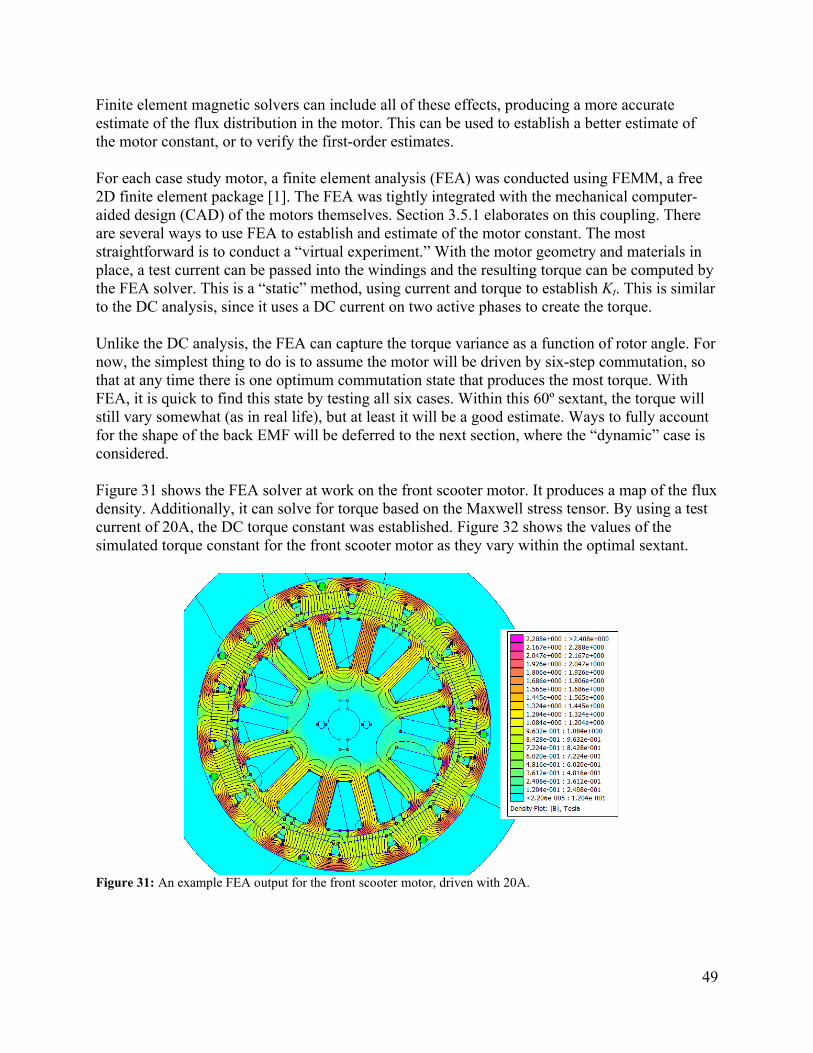
49

Finite element magnetic solvers can include all of these effects, producing a more accurate estimate of the flux distribution in the motor. This can be used to establish a better estimate of the motor constant, or to verify the first-order estimates.

For each case study motor, a finite element analysis (FEA) was conducted using FEMM, a free 2D finite element package [1]. The FEA was tightly integrated with the mechanical computer-aided design (CAD) of the motors themselves. Section 3.5.1 elaborates on this coupling. There are several ways to use FEA to establish and estimate of the motor constant. The most straightforward is to conduct a “virtual experiment.” With the motor geometry and materials in place, a test current can be passed into the windings and the resulting torque can be computed by the FEA solver. This is a “static” method, using current and torque to establish Kt. This is similar to the DC analysis, since it uses a DC current on two active phases to create the torque.

Unlike the DC analysis, the FEA can capture the torque variance as a function of rotor angle. For now, the simplest thing to do is to assume the motor will be driven by six-step commutation, so that at any time there is one optimum commutation state that produces the most torque. With FEA, it is quick to find this state by testing all six cases. Within this 60º sextant, the torque will still vary somewhat (as in real life), but at least it will be a good estimate. Ways to fully account for the shape of the back EMF will be deferred to the next section, where the “dynamic” case is considered.

Figure 31 shows the FEA solver at work on the front scooter motor. It produces a map of the flux density. Additionally, it can solve for torque based on the Maxwell stress tensor. By using a test current of 20A, the DC torque constant was established. Figure 32 shows the values of the simulated torque constant for the front scooter motor as they vary within the optimal sextant.

Figure 31: An example FEA output for the front scooter motor, driven with 20A.

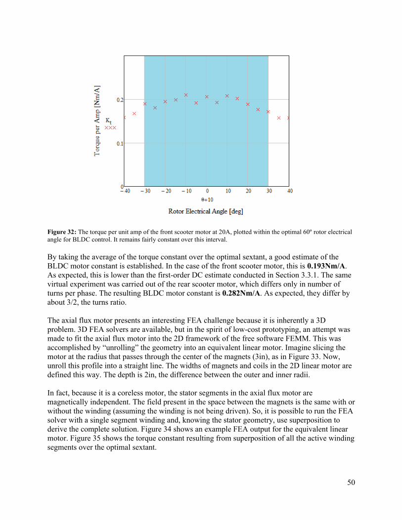
50

Figure 32: The torque per unit amp of the front scooter motor at 20A, plotted within the optimal 60º rotor electrical angle for BLDC control. It remains fairly constant over this interval.

By taking the average of the torque constant over the optimal sextant, a good estimate of the BLDC motor constant is established. In the case of the front scooter motor, this is 0.193Nm/A. As expected, this is lower than the first-order DC estimate conducted in Section 3.3.1. The same virtual experiment was carried out of the rear scooter motor, which differs only in number of turns per phase. The resulting BLDC motor constant is 0.282Nm/A. As expected, they differ by about 3/2, the turns ratio.

The axial flux motor presents an interesting FEA challenge because it is inherently a 3D problem. 3D FEA solvers are available, but in the spirit of low-cost prototyping, an attempt was made to fit the axial flux motor into the 2D framework of the free software FEMM. This was accomplished by “unrolling” the geometry into an equivalent linear motor. Imagine slicing the motor at the radius that passes through the center of the magnets (3in), as in Figure 33. Now, unroll this profile into a straight line. The widths of magnets and coils in the 2D linear motor are defined this way. The depth is 2in, the difference between the outer and inner radii.

In fact, because it is a coreless motor, the stator segments in the axial flux motor are magnetically independent. The field present in the space between the magnets is the same with or without the winding (assuming the winding is not being driven). So, it is possible to run the FEA solver with a single segment winding and, knowing the stator geometry, use superposition to derive the complete solution. Figure 34 shows an example FEA output for the equivalent linear motor. Figure 35 shows the torque constant resulting from superposition of all the active winding segments over the optimal sextant.

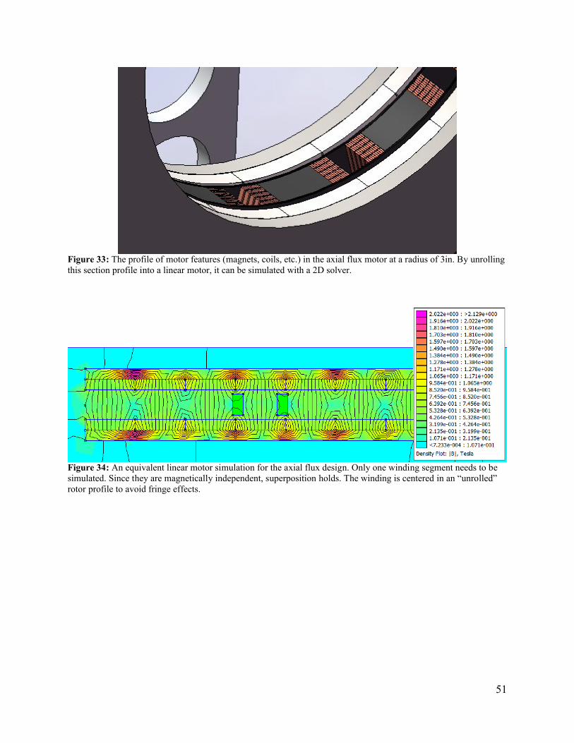
51

Figure 33: The profile of motor features (magnets, coils, etc.) in the axial flux motor at a radius of 3in. By unrolling this section profile into a linear motor, it can be simulated with a 2D solver.

Figure 34: An equivalent linear motor simulation for the axial flux design. Only one winding segment needs to be simulated. Since they are magnetically independent, superposition holds. The winding is centered in an “unrolled” rotor profile to avoid fringe effects.

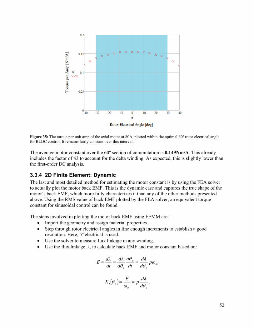
52

Figure 35: The torque per unit amp of the axial motor at 80A, plotted within the optimal 60º rotor electrical angle for BLDC control. It remains fairly constant over this interval.

The average motor constant over the 60º section of commutation is 0.149Nm/A. This already includes the factor of √3 to account for the delta winding. As expected, this is slightly lower than the first-order DC analysis.

3.3.4 2D Finite Element: Dynamic The last and most detailed method for estimating the motor constant is by using the FEA solver to actually plot the motor back EMF. This is the dynamic case and captures the true shape of the motor’s back EMF, which more fully characterizes it than any of the other methods presented above. Using the RMS value of back EMF plotted by the FEA solver, an equivalent torque constant for sinusoidal control can be found.

The steps involved in plotting the motor back EMF using FEMM are: Import the geometry and assign material properties. Step through rotor electrical angles in fine enough increments to establish a good

resolution. Here, 5º electrical is used. Use the solver to measure flux linkage in any winding. Use the flux linkage, λ, to calculate back EMF and motor constant based on:

me

e

e

pd

d

dt

d

d

d

dt

dE

em

et d

dp

EK

.

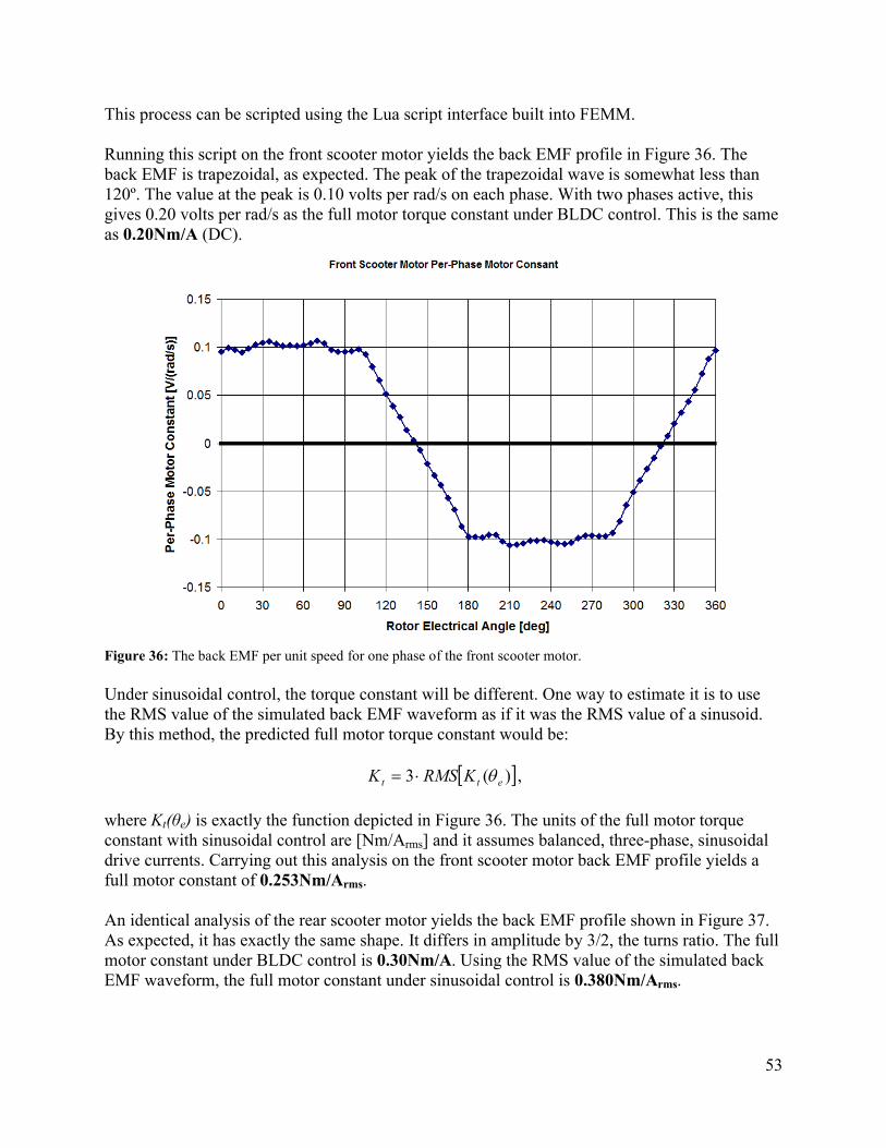
53

This process can be scripted using the Lua script interface built into FEMM.

Running this script on the front scooter motor yields the back EMF profile in Figure 36. The back EMF is trapezoidal, as expected. The peak of the trapezoidal wave is somewhat less than 120º. The value at the peak is 0.10 volts per rad/s on each phase. With two phases active, this gives 0.20 volts per rad/s as the full motor torque constant under BLDC control. This is the same as 0.20Nm/A (DC).

Figure 36: The back EMF per unit speed for one phase of the front scooter motor.

Under sinusoidal control, the torque constant will be different. One way to estimate it is to use the RMS value of the simulated back EMF waveform as if it was the RMS value of a sinusoid. By this method, the predicted full motor torque constant would be:

)(3 ett KRMSK ,

where Kt(θe) is exactly the function depicted in Figure 36. The units of the full motor torque constant with sinusoidal control are [Nm/Arms] and it assumes balanced, three-phase, sinusoidal drive currents. Carrying out this analysis on the front scooter motor back EMF profile yields a full motor constant of 0.253Nm/Arms.

An identical analysis of the rear scooter motor yields the back EMF profile shown in Figure 37. As expected, it has exactly the same shape. It differs in amplitude by 3/2, the turns ratio. The full motor constant under BLDC control is 0.30Nm/A. Using the RMS value of the simulated back EMF waveform, the full motor constant under sinusoidal control is 0.380Nm/Arms.

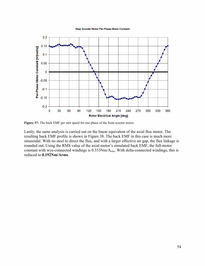
54

Figure 37: The back EMF per unit speed for one phase of the front scooter motor.

Lastly, the same analysis is carried out on the linear equivalent of the axial flux motor. The resulting back EMF profile is shown in Figure 38. The back EMF in this case is much more sinusoidal. With no steel to direct the flux, and with a larger effective air gap, the flux linkage is rounded out. Using the RMS value of the axial motor’s simulated back EMF, the full-motor constant with wye-connected windings is 0.333Nm/Arms. With delta-connected windings, this is reduced to 0.192Nm/Arms.

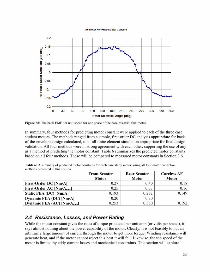
55

Figure 38: The back EMF per unit speed for one phase of the coreless axial flux motor.

In summary, four methods for predicting motor constant were applied to each of the three case student motors. The methods ranged from a simple, first-order DC analysis appropriate for back-of-the-envelope design calculated, to a full finite element simulation appropriate for final design validation. All four methods were in strong agreement with each other, supporting the use of any as a method of predicting the motor constant. Table 6 summarizes the predicted motor constants based on all four methods. These will be compared to measured motor constants in Section 3.6.

Table 6: A summary of predicted motor constants for each case study motor, using all four motor prediction methods presented in this section.

Front Scooter Motor

Rear Scooter Motor

Coreless AF Motor

First-Order DC [Nm/A] 0.27 0.40 0.18First-Order AC [Nm/Arms] 0.25 0.37 0.16Static FEA (DC) [Nm/A] 0.193 0.282 0.149Dynamic FEA (DC) [Nm/A]Dynamic FEA (AC) [Nm/Arms]

0.200.253

0.300.380 0.192

3.4 Resistance, Losses, and Power RatingWhile the motor constant gives the ratio of torque produced per unit amp (or volts per speed), it says almost nothing about the power capability of the motor. Clearly, it is not feasibly to put an arbitrarily large amount of current through the motor to get more torque. Winding resistance will generate heat, and if the motor cannot reject this heat it will fail. Likewise, the top speed of the motor is limited by eddy current losses and mechanical constraints. This section will explore

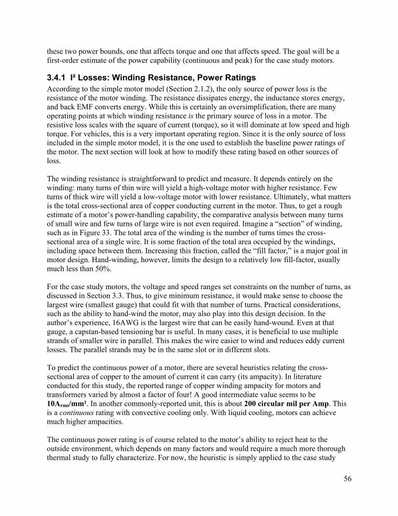
56

these two power bounds, one that affects torque and one that affects speed. The goal will be a first-order estimate of the power capability (continuous and peak) for the case study motors.

3.4.1 I² Losses: Winding Resistance, Power RatingsAccording to the simple motor model (Section 2.1.2), the only source of power loss is the resistance of the motor winding. The resistance dissipates energy, the inductance stores energy, and back EMF converts energy. While this is certainly an oversimplification, there are many operating points at which winding resistance is the primary source of loss in a motor. The resistive loss scales with the square of current (torque), so it will dominate at low speed and high torque. For vehicles, this is a very important operating region. Since it is the only source of loss included in the simple motor model, it is the one used to establish the baseline power ratings of the motor. The next section will look at how to modify these rating based on other sources of loss.

The winding resistance is straightforward to predict and measure. It depends entirely on the winding: many turns of thin wire will yield a high-voltage motor with higher resistance. Few turns of thick wire will yield a low-voltage motor with lower resistance. Ultimately, what matters is the total cross-sectional area of copper conducting current in the motor. Thus, to get a rough estimate of a motor’s power-handling capability, the comparative analysis between many turns of small wire and few turns of large wire is not even required. Imagine a “section” of winding, such as in Figure 33. The total area of the winding is the number of turns times the cross-sectional area of a single wire. It is some fraction of the total area occupied by the windings, including space between them. Increasing this fraction, called the “fill factor,” is a major goal in motor design. Hand-winding, however, limits the design to a relatively low fill-factor, usually much less than 50%.

For the case study motors, the voltage and speed ranges set constraints on the number of turns, as discussed in Section 3.3. Thus, to give minimum resistance, it would make sense to choose the largest wire (smallest gauge) that could fit with that number of turns. Practical considerations, such as the ability to hand-wind the motor, may also play into this design decision. In the author’s experience, 16AWG is the largest wire that can be easily hand-wound. Even at that gauge, a capstan-based tensioning bar is useful. In many cases, it is beneficial to use multiple strands of smaller wire in parallel. This makes the wire easier to wind and reduces eddy current losses. The parallel strands may be in the same slot or in different slots.

To predict the continuous power of a motor, there are several heuristics relating the cross-sectional area of copper to the amount of current it can carry (its ampacity). In literature conducted for this study, the reported range of copper winding ampacity for motors and transformers varied by almost a factor of four! A good intermediate value seems to be 10Arms/mm². In another commonly-reported unit, this is about 200 circular mil per Amp. This is a continuous rating with convective cooling only. With liquid cooling, motors can achieve much higher ampacities.

The continuous power rating is of course related to the motor’s ability to reject heat to the outside environment, which depends on many factors and would require a much more thorough thermal study to fully characterize. For now, the heuristic is simply applied to the case study

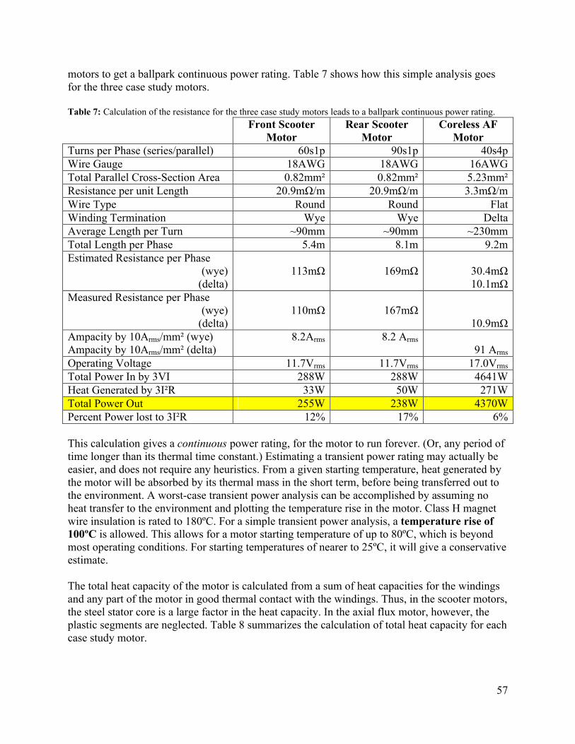
57

motors to get a ballpark continuous power rating. Table 7 shows how this simple analysis goes for the three case study motors.

Table 7: Calculation of the resistance for the three case study motors leads to a ballpark continuous power rating.

Front Scooter Motor

Rear Scooter Motor

Coreless AF Motor

Turns per Phase (series/parallel) 60s1p 90s1p 40s4pWire Gauge 18AWG 18AWG 16AWGTotal Parallel Cross-Section Area 0.82mm² 0.82mm² 5.23mm²Resistance per unit Length 20.9mΩ/m 20.9mΩ/m 3.3mΩ/mWire Type Round Round FlatWinding Termination Wye Wye DeltaAverage Length per Turn ~90mm ~90mm ~230mmTotal Length per Phase 5.4m 8.1m 9.2mEstimated Resistance per Phase

(wye)(delta)

113mΩ 169mΩ 30.4mΩ10.1mΩ

Measured Resistance per Phase(wye)

(delta)110mΩ 167mΩ

10.9mΩAmpacity by 10Arms/mm² (wye)Ampacity by 10Arms/mm² (delta)

8.2Arms 8.2 Arms

91 Arms

Operating Voltage 11.7Vrms 11.7Vrms 17.0Vrms

Total Power In by 3VI 288W 288W 4641WHeat Generated by 3I²R 33W 50W 271WTotal Power Out 255W 238W 4370WPercent Power lost to 3I²R 12% 17% 6%

This calculation gives a continuous power rating, for the motor to run forever. (Or, any period of time longer than its thermal time constant.) Estimating a transient power rating may actually be easier, and does not require any heuristics. From a given starting temperature, heat generated by the motor will be absorbed by its thermal mass in the short term, before being transferred out to the environment. A worst-case transient power analysis can be accomplished by assuming no heat transfer to the environment and plotting the temperature rise in the motor. Class H magnet wire insulation is rated to 180ºC. For a simple transient power analysis, a temperature rise of 100ºC is allowed. This allows for a motor starting temperature of up to 80ºC, which is beyond most operating conditions. For starting temperatures of nearer to 25ºC, it will give a conservative estimate.

The total heat capacity of the motor is calculated from a sum of heat capacities for the windings and any part of the motor in good thermal contact with the windings. Thus, in the scooter motors, the steel stator core is a large factor in the heat capacity. In the axial flux motor, however, the plastic segments are neglected. Table 8 summarizes the calculation of total heat capacity for each case study motor.

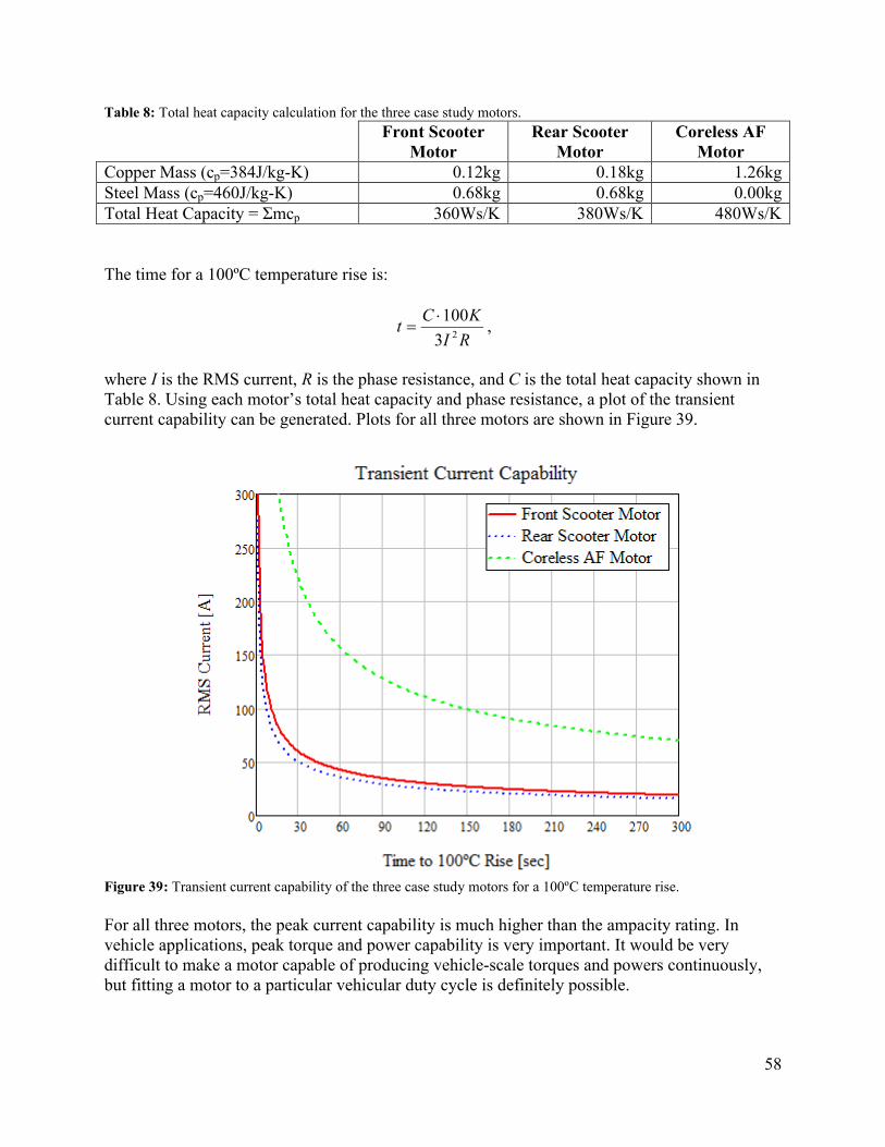
58

Table 8: Total heat capacity calculation for the three case study motors.

Front Scooter Motor

Rear Scooter Motor

Coreless AF Motor

Copper Mass (cp=384J/kg-K) 0.12kg 0.18kg 1.26kgSteel Mass (cp=460J/kg-K) 0.68kg 0.68kg 0.00kgTotal Heat Capacity = Σmcp 360Ws/K 380Ws/K 480Ws/K

The time for a 100ºC temperature rise is:

RI

KCt

23

100 ,

where I is the RMS current, R is the phase resistance, and C is the total heat capacity shown in Table 8. Using each motor’s total heat capacity and phase resistance, a plot of the transient current capability can be generated. Plots for all three motors are shown in Figure 39.

Figure 39: Transient current capability of the three case study motors for a 100ºC temperature rise.

For all three motors, the peak current capability is much higher than the ampacity rating. In vehicle applications, peak torque and power capability is very important. It would be very difficult to make a motor capable of producing vehicle-scale torques and powers continuously, but fitting a motor to a particular vehicular duty cycle is definitely possible.

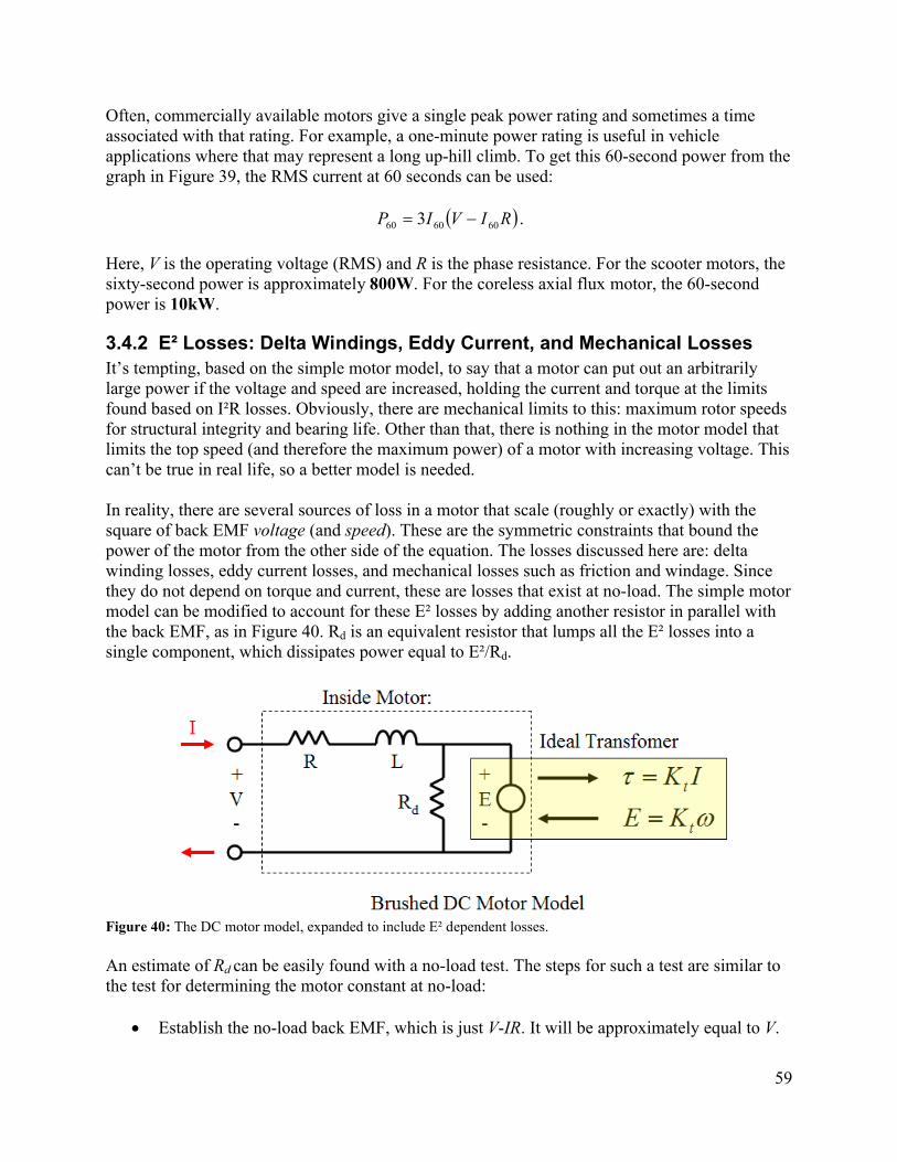
59

Often, commercially available motors give a single peak power rating and sometimes a time associated with that rating. For example, a one-minute power rating is useful in vehicle applications where that may represent a long up-hill climb. To get this 60-second power from the graph in Figure 39, the RMS current at 60 seconds can be used:

RIVIP 606060 3 .

Here, V is the operating voltage (RMS) and R is the phase resistance. For the scooter motors, the sixty-second power is approximately 800W. For the coreless axial flux motor, the 60-second power is 10kW.

3.4.2 E² Losses: Delta Windings, Eddy Current, and Mechanical LossesIt’s tempting, based on the simple motor model, to say that a motor can put out an arbitrarily large power if the voltage and speed are increased, holding the current and torque at the limits found based on I²R losses. Obviously, there are mechanical limits to this: maximum rotor speeds for structural integrity and bearing life. Other than that, there is nothing in the motor model that limits the top speed (and therefore the maximum power) of a motor with increasing voltage. This can’t be true in real life, so a better model is needed.

In reality, there are several sources of loss in a motor that scale (roughly or exactly) with the square of back EMF voltage (and speed). These are the symmetric constraints that bound the power of the motor from the other side of the equation. The losses discussed here are: delta winding losses, eddy current losses, and mechanical losses such as friction and windage. Since they do not depend on torque and current, these are losses that exist at no-load. The simple motor model can be modified to account for these E² losses by adding another resistor in parallel with the back EMF, as in Figure 40. Rd is an equivalent resistor that lumps all the E² losses into a single component, which dissipates power equal to E²/Rd.

Figure 40: The DC motor model, expanded to include E² dependent losses.

An estimate of Rd can be easily found with a no-load test. The steps for such a test are similar to the test for determining the motor constant at no-load:

Establish the no-load back EMF, which is just V-IR. It will be approximately equal to V.

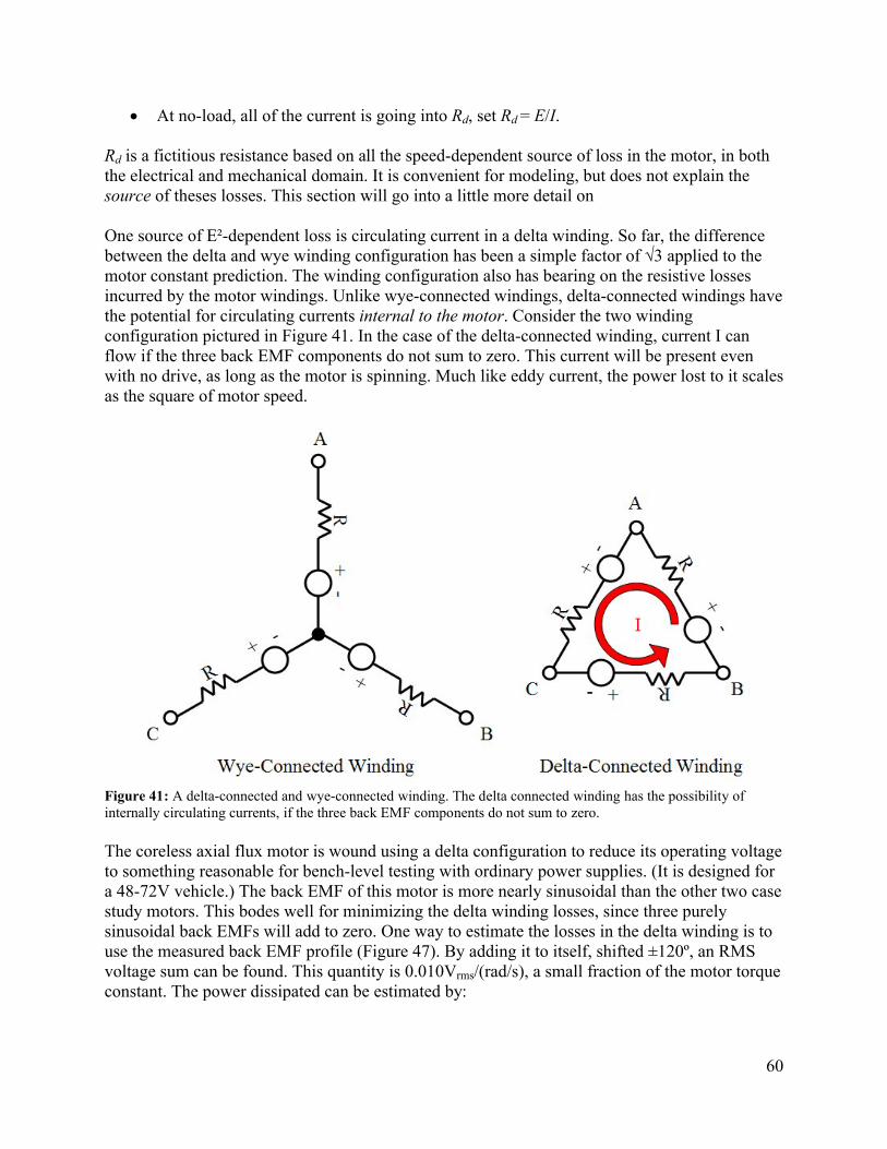
60

At no-load, all of the current is going into Rd, set Rd = E/I.

Rd is a fictitious resistance based on all the speed-dependent source of loss in the motor, in both the electrical and mechanical domain. It is convenient for modeling, but does not explain the source of theses losses. This section will go into a little more detail on

One source of E²-dependent loss is circulating current in a delta winding. So far, the difference between the delta and wye winding configuration has been a simple factor of √3 applied to the motor constant prediction. The winding configuration also has bearing on the resistive losses incurred by the motor windings. Unlike wye-connected windings, delta-connected windings have the potential for circulating currents internal to the motor. Consider the two winding configuration pictured in Figure 41. In the case of the delta-connected winding, current I can flow if the three back EMF components do not sum to zero. This current will be present even with no drive, as long as the motor is spinning. Much like eddy current, the power lost to it scales as the square of motor speed.

Figure 41: A delta-connected and wye-connected winding. The delta connected winding has the possibility ofinternally circulating currents, if the three back EMF components do not sum to zero.

The coreless axial flux motor is wound using a delta configuration to reduce its operating voltage to something reasonable for bench-level testing with ordinary power supplies. (It is designed for a 48-72V vehicle.) The back EMF of this motor is more nearly sinusoidal than the other two case study motors. This bodes well for minimizing the delta winding losses, since three purely sinusoidal back EMFs will add to zero. One way to estimate the losses in the delta winding is to use the measured back EMF profile (Figure 47). By adding it to itself, shifted ±120º, an RMS voltage sum can be found. This quantity is 0.010Vrms/(rad/s), a small fraction of the motor torque constant. The power dissipated can be estimated by:

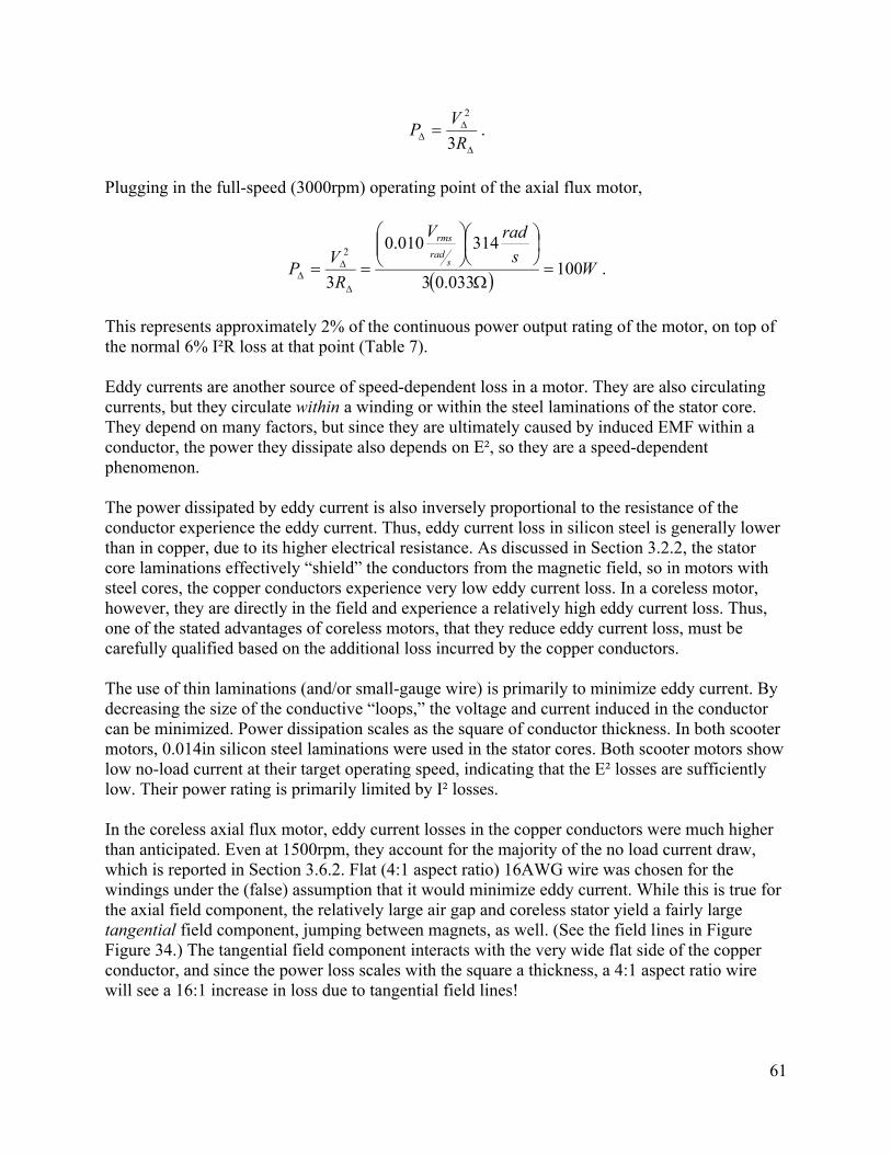
61

R

VP

3

2

.

Plugging in the full-speed (3000rpm) operating point of the axial flux motor,

Ws

radV

R

VP s

rad

rms

100033.03

314010.0

3

2

.

This represents approximately 2% of the continuous power output rating of the motor, on top of the normal 6% I²R loss at that point (Table 7).

Eddy currents are another source of speed-dependent loss in a motor. They are also circulating currents, but they circulate within a winding or within the steel laminations of the stator core. They depend on many factors, but since they are ultimately caused by induced EMF within a conductor, the power they dissipate also depends on E², so they are a speed-dependent phenomenon.

The power dissipated by eddy current is also inversely proportional to the resistance of the conductor experience the eddy current. Thus, eddy current loss in silicon steel is generally lower than in copper, due to its higher electrical resistance. As discussed in Section 3.2.2, the stator core laminations effectively “shield” the conductors from the magnetic field, so in motors with steel cores, the copper conductors experience very low eddy current loss. In a coreless motor, however, they are directly in the field and experience a relatively high eddy current loss. Thus, one of the stated advantages of coreless motors, that they reduce eddy current loss, must be carefully qualified based on the additional loss incurred by the copper conductors.

The use of thin laminations (and/or small-gauge wire) is primarily to minimize eddy current. By decreasing the size of the conductive “loops,” the voltage and current induced in the conductor can be minimized. Power dissipation scales as the square of conductor thickness. In both scooter motors, 0.014in silicon steel laminations were used in the stator cores. Both scooter motors show low no-load current at their target operating speed, indicating that the E² losses are sufficiently low. Their power rating is primarily limited by I² losses.

In the coreless axial flux motor, eddy current losses in the copper conductors were much higher than anticipated. Even at 1500rpm, they account for the majority of the no load current draw, which is reported in Section 3.6.2. Flat (4:1 aspect ratio) 16AWG wire was chosen for the windings under the (false) assumption that it would minimize eddy current. While this is true for the axial field component, the relatively large air gap and coreless stator yield a fairly large tangential field component, jumping between magnets, as well. (See the field lines in Figure Figure 34.) The tangential field component interacts with the very wide flat side of the copper conductor, and since the power loss scales with the square a thickness, a 4:1 aspect ratio wire will see a 16:1 increase in loss due to tangential field lines!

62

Other speed-dependent losses are mechanical in nature. Coulomb friction aside, most sources of drag and damping increase with the speed of the motor. Viscous drag in the bearings is one example. Windage, which is aerodynamic drag in the air gap, is another. Modeling these as an E²-dependent loss is a very rough approximation, but the simplicity it offers in modeling can be good at the early design stage. More thorough simulation in the mechanical domain would be needed to get a better estimate of these losses.

Speed-dependent losses are generally harder to predict than the simple I² resistive losses. For this reason, they are often determined experimentally by solving for Rd or parameters in a more complete loss model. They can play a significant role in the power rating of a motor. For example, the axial flux motor, as tested in this case study, would ultimately be limited more by eddy current losses than normal resistive losses. In many situations, though, speed-dependent losses are mitigated by additional cooling accomplished by integrated fans, or by channeling air from a moving vehicle over the motor. In other words, the extra heat from these losses is more easily removed than the heat generated at low speed by I2R.

No single number can capture the power generating capability or efficiency of a motor. The motor and system must be modeled together to establish the safe operating area and an efficiency map. (Each will be a function of time, duty cycle, ambient temperature, etc.) In motors that are designed for variable speed operation, such as for traction applications, the drive cycle is as much an important factor in determining the power capability of the motor as the intrinsic motor properties discussed here.

3.5 Motor Prototyping MethodsIn the above sections, the focus has been on predicting motor performance using analysis and simulation. The next phase of design involves fabrication and evaluation of an actual motor prototype. This section will discuss methods that are useful for prototype motor fabrication. Knowing which parts of the fabrication to do in-house and which to send out is important and specific to each individual build. The deciding factors might include available machinery, required precision, and of course, time/money. Methods emphasized here are low-cost, short cycle techniques that can be used in labs (or by individuals) for which motor design is not the primary focus.

3.5.1 Integrated CAD/FEA/CAMThe design cycle of a prototype motor build can be significantly reduced by integrating computational resources. These include computer-aided mechanical design, mechanical FEA, electromagnetic FEA, and computer-aided manufacturing. Many software packages allow sharing of common file types, such as the .dxf-format drawing. By jumping between mechanical and electromagnetic computer-aided design, problems that cross between the two domains become evident and can be solved before fabrication.

One example of this interaction is the placement of bolt holes in the scooter motors. Figure 42shows the general construction of each scooter motor. The scooter motors were designed in the SolidWorks CAD software. The rotor (which is the outside ring of the motor, in this case) is captured by two side plates that hold the bearings. To fasten these side plates, a through-bolt pattern allows long machine screws to pass through the two plates and the rotor ring.

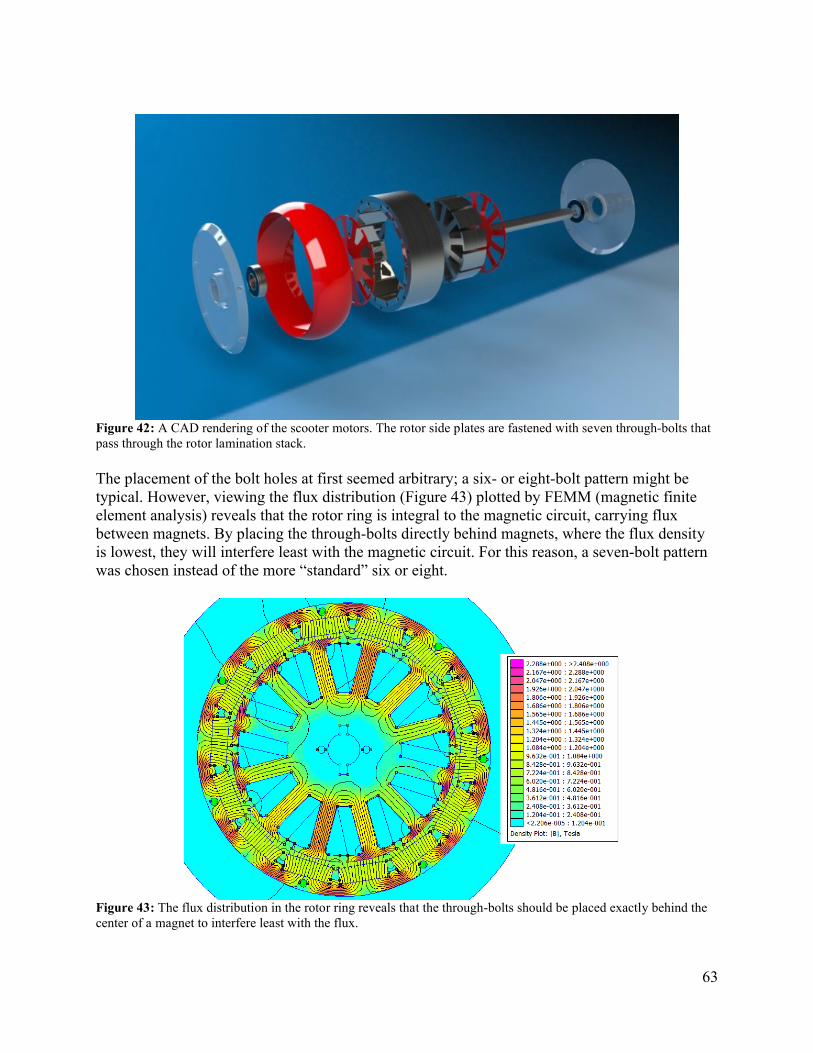
63

Figure 42: A CAD rendering of the scooter motors. The rotor side plates are fastened with seven through-bolts that pass through the rotor lamination stack.

The placement of the bolt holes at first seemed arbitrary; a six- or eight-bolt pattern might be typical. However, viewing the flux distribution (Figure 43) plotted by FEMM (magnetic finite element analysis) reveals that the rotor ring is integral to the magnetic circuit, carrying flux between magnets. By placing the through-bolts directly behind magnets, where the flux density is lowest, they will interfere least with the magnetic circuit. For this reason, a seven-bolt pattern was chosen instead of the more “standard” six or eight.

Figure 43: The flux distribution in the rotor ring reveals that the through-bolts should be placed exactly behind the center of a magnet to interfere least with the flux.

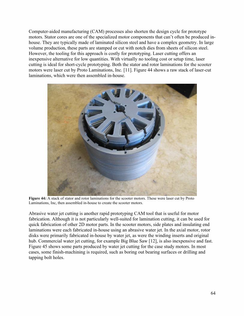
64

Computer-aided manufacturing (CAM) processes also shorten the design cycle for prototype motors. Stator cores are one of the specialized motor components that can’t often be produced in-house. They are typically made of laminated silicon steel and have a complex geometry. In large volume production, these parts are stamped or cut with notch dies from sheets of silicon steel. However, the tooling for this approach is costly for prototyping. Laser cutting offers an inexpensive alternative for low quantities. With virtually no tooling cost or setup time, laser cutting is ideal for short-cycle prototyping. Both the stator and rotor laminations for the scooter motors were laser cut by Proto Laminations, Inc. [11]. Figure 44 shows a raw stack of laser-cut laminations, which were then assembled in-house.

Figure 44: A stack of stator and rotor laminations for the scooter motors. These were laser cut by Proto Laminations, Inc, then assembled in-house to create the scooter motors.

Abrasive water jet cutting is another rapid prototyping CAM tool that is useful for motor fabrication. Although it is not particularly well-suited for lamination cutting, it can be used for quick fabrication of other 2D motor parts. In the scooter motors, side plates and insulating end laminations were each fabricated in-house using an abrasive water jet. In the axial motor, rotor disks were primarily fabricated in-house by water jet, as were the winding inserts and original hub. Commercial water jet cutting, for example Big Blue Saw [12], is also inexpensive and fast. Figure 45 shows some parts produced by water jet cutting for the case study motors. In most cases, some finish-machining is required, such as boring out bearing surfaces or drilling and tapping bolt holes.

65

Figure 45: Part produced by abrasive water jet (with some finish machining): Insulating end laminations (top left), side plates (top right and bottom left), and winding inserts (bottom right).

3.5.2 Design for Assembly (and Disassembly)For motor prototypes that will be built in-house, designing for ease of assembly and disassembly is very important. Two processes where this is most evident are winding and final rotor/stator assembly. Both of these processes, if not carefully considered and designed for, can require more force or dexterity than is possible in hand fabrication. These processes can also ruin a design if done incorrectly and irreversibly. This section presents a small set of techniques that can be helpful in optimizing a motor design for in-house hand assembly.

Winding a motor by hand can be extremely difficult, and although it may not be the most time-consuming process of motor fabrication, but it will always seem that way! Design with this in mind. For a prototype motor, anticipating a lower packing density is one way to avoid disappointment. The scooter motors utilize only a small fraction of the available slot space for winding, but since this was planned they still perform to specification. In most cases, though, this is contradictory to the goal of optimizing power density. To pack as much winding into slots as possible, a simple tensioning jig, such as wrapping the wire around a round object, can make a huge difference. Using multiple strands of smaller wire will reduce the bend radii as well, allowing more total windings to fit in the slot.

Some kind of core insulation is crucial. Winding around sharp metal corners will break the thin enamel insulation of the magnet wire, causing shorts. In the scooter motors, fiberglass end

66

laminations (pictured in Figure 45) were used to protect windings from the corners of the stator core. Before final assembly, it is still important to test windings for shorts to each other and to the stator core.

Certain types of motor are much easier to wind by hand than others. Outside-rotor motors, such as the scooter motors, are much easier to wind because the stator slots face outward. Thus, wire can be simply dropped through spaces between stator teeth. For inside-rotor motors, the entire wire spool needs to be threaded through the stator for each turn. The axial flux motor design was also chosen particularly for its amenability to hand winding. Each stator segment can be removed, wound in open space, and re-inserted. After that, only a few solder joints are required for interconnections.

Final assembly, when the rotor and stator are put together, is also an important step for which planning is crucial. The magnetic attraction between the stator and rotor can be very strong, making it difficult (and possibly dangerous) to align parts as they come together. Depending on the size of the motor, an assembly jig may be required. For the scooter motors, using a drill press to hold and align the parts during assembly was sufficient. In the case of the axial motor, there is no force between the rotor and stator, but the axial force between rotor disks is nearly 500lbf. To assemble this motor, a simple jig (shown in Figure 46) was constructed that could safely and slowly lower one rotor disk onto the stator and second rotor disks using threaded lead screws.

Allowing for disassembly is very important in motor prototyping. In both case studies, motors had to be disassembled due to fabrication or winding mistakes. The scooter motors were small enough to be disassembled by hand. For the axial motor, the same jig used for assembly of the axial motor could be used to pull the two disks apart. Using adhesives to seal the motor or epoxy to fix windings is a good idea, but it should only be done after testing has revealed the motor to be working.

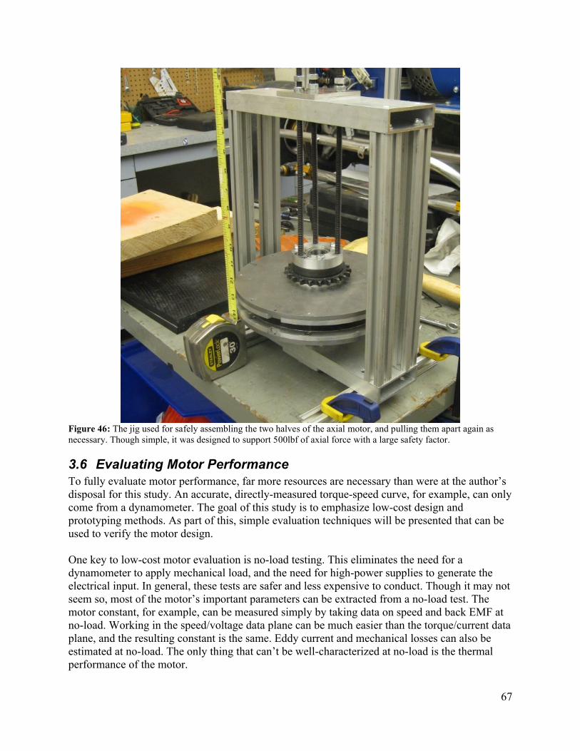
67

Figure 46: The jig used for safely assembling the two halves of the axial motor, and pulling them apart again as necessary. Though simple, it was designed to support 500lbf of axial force with a large safety factor.

3.6 Evaluating Motor PerformanceTo fully evaluate motor performance, far more resources are necessary than were at the author’s disposal for this study. An accurate, directly-measured torque-speed curve, for example, can only come from a dynamometer. The goal of this study is to emphasize low-cost design and prototyping methods. As part of this, simple evaluation techniques will be presented that can be used to verify the motor design.

One key to low-cost motor evaluation is no-load testing. This eliminates the need for a dynamometer to apply mechanical load, and the need for high-power supplies to generate the electrical input. In general, these tests are safer and less expensive to conduct. Though it may not seem so, most of the motor’s important parameters can be extracted from a no-load test. The motor constant, for example, can be measured simply by taking data on speed and back EMF at no-load. Working in the speed/voltage data plane can be much easier than the torque/current data plane, and the resulting constant is the same. Eddy current and mechanical losses can also be estimated at no-load. The only thing that can’t be well-characterized at no-load is the thermal performance of the motor.

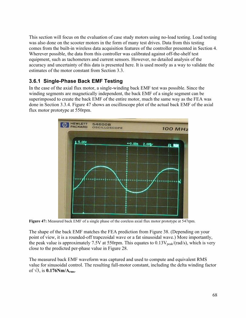
68

This section will focus on the evaluation of case study motors using no-load testing. Load testing was also done on the scooter motors in the form of many test drives. Data from this testing comes from the built-in wireless data acquisition features of the controller presented in Section 4. Wherever possible, the data from this controller was calibrated against off-the-shelf test equipment, such as tachometers and current sensors. However, no detailed analysis of the accuracy and uncertainty of this data is presented here. It is used mostly as a way to validate the estimates of the motor constant from Section 3.3.

3.6.1 Single-Phase Back EMF TestingIn the case of the axial flux motor, a single-winding back EMF test was possible. Since the winding segments are magnetically independent, the back EMF of a single segment can be superimposed to create the back EMF of the entire motor, much the same way as the FEA was done in Section 3.3.4. Figure 47 shows an oscilloscope plot of the actual back EMF of the axial flux motor prototype at 550rpm.

Figure 47: Measured back EMF of a single phase of the coreless axial flux motor prototype at 547rpm.

The shape of the back EMF matches the FEA prediction from Figure 38. (Depending on your point of view, it is a rounded-off trapezoidal wave or a fat sinusoidal wave.) More importantly, the peak value is approximately 7.5V at 550rpm. This equates to 0.13Vpeak/(rad/s), which is very close to the predicted per-phase value in Figure 28.

The measured back EMF waveform was captured and used to compute and equivalent RMS value for sinusoidal control. The resulting full-motor constant, including the delta winding factor of √3, is 0.176Nm/Arms.

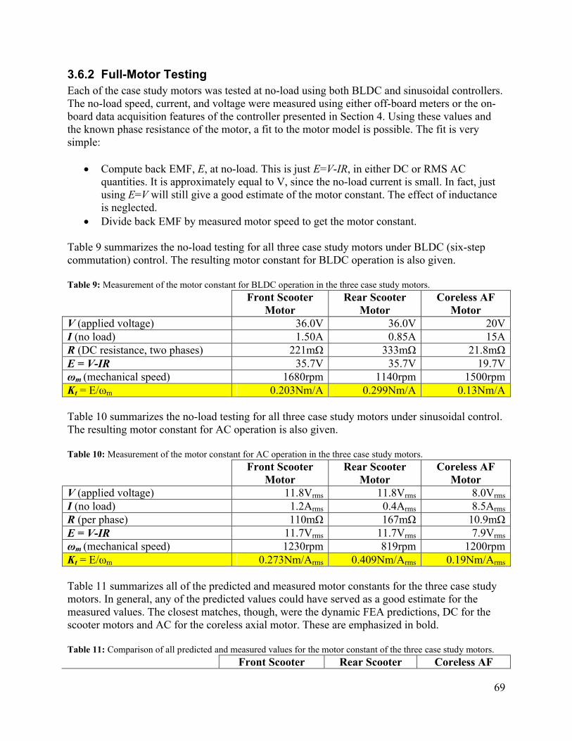
69

3.6.2 Full-Motor TestingEach of the case study motors was tested at no-load using both BLDC and sinusoidal controllers. The no-load speed, current, and voltage were measured using either off-board meters or the on-board data acquisition features of the controller presented in Section 4. Using these values and the known phase resistance of the motor, a fit to the motor model is possible. The fit is very simple:

Compute back EMF, E, at no-load. This is just E=V-IR, in either DC or RMS AC quantities. It is approximately equal to V, since the no-load current is small. In fact, just using E=V will still give a good estimate of the motor constant. The effect of inductance is neglected.

Divide back EMF by measured motor speed to get the motor constant.

Table 9 summarizes the no-load testing for all three case study motors under BLDC (six-step commutation) control. The resulting motor constant for BLDC operation is also given.

Table 9: Measurement of the motor constant for BLDC operation in the three case study motors.

Front Scooter Motor

Rear Scooter Motor

Coreless AF Motor

V (applied voltage) 36.0V 36.0V 20VI (no load) 1.50A 0.85A 15AR (DC resistance, two phases) 221mΩ 333mΩ 21.8mΩE = V-IR 35.7V 35.7V 19.7Vωm (mechanical speed) 1680rpm 1140rpm 1500rpmKt = E/ωm 0.203Nm/A 0.299Nm/A 0.13Nm/A

Table 10 summarizes the no-load testing for all three case study motors under sinusoidal control. The resulting motor constant for AC operation is also given.

Table 10: Measurement of the motor constant for AC operation in the three case study motors.

Front Scooter Motor

Rear Scooter Motor

Coreless AF Motor

V (applied voltage) 11.8Vrms 11.8Vrms 8.0Vrms

I (no load) 1.2Arms 0.4Arms 8.5Arms

R (per phase) 110mΩ 167mΩ 10.9mΩE = V-IR 11.7Vrms 11.7Vrms 7.9Vrms

ωm (mechanical speed) 1230rpm 819rpm 1200rpmKt = E/ωm 0.273Nm/Arms 0.409Nm/Arms 0.19Nm/Arms

Table 11 summarizes all of the predicted and measured motor constants for the three case study motors. In general, any of the predicted values could have served as a good estimate for the measured values. The closest matches, though, were the dynamic FEA predictions, DC for the scooter motors and AC for the coreless axial motor. These are emphasized in bold.

Table 11: Comparison of all predicted and measured values for the motor constant of the three case study motors.

Front Scooter Rear Scooter Coreless AF

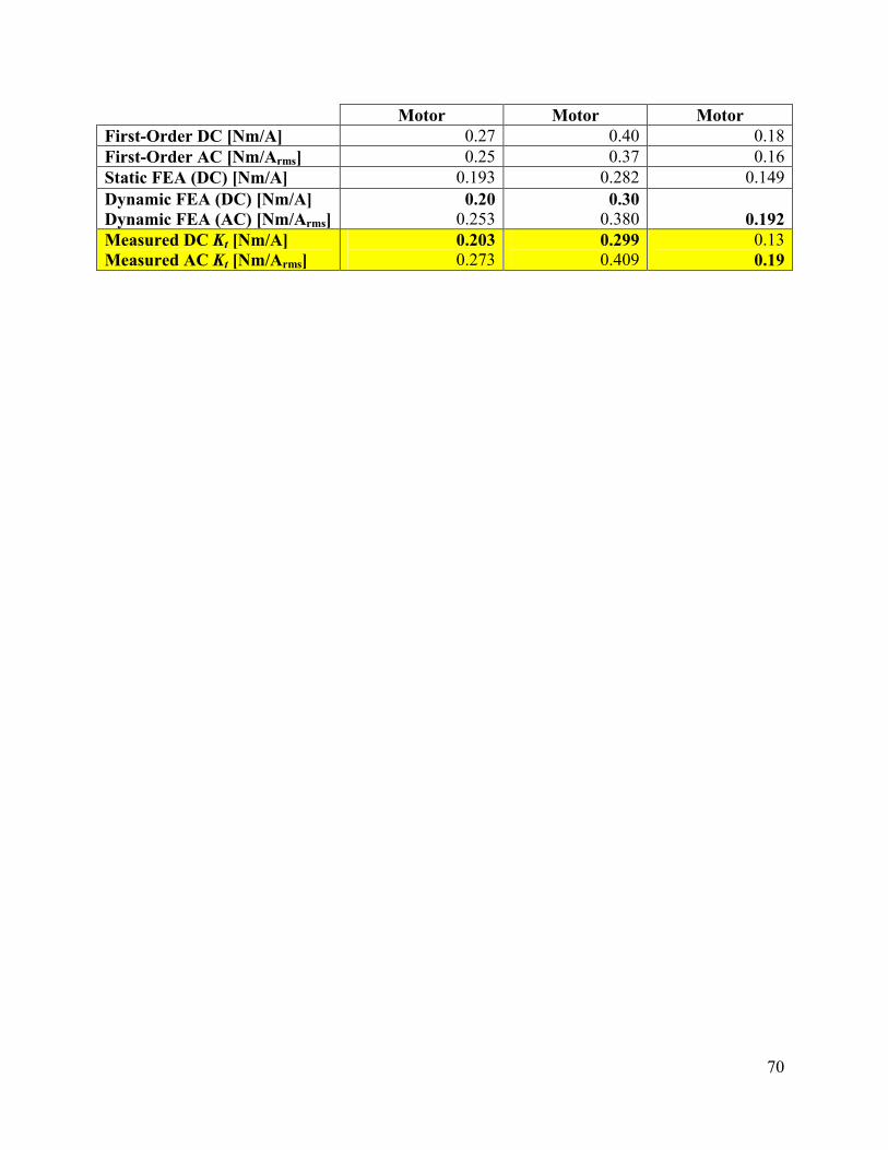
70

Motor Motor MotorFirst-Order DC [Nm/A] 0.27 0.40 0.18First-Order AC [Nm/Arms] 0.25 0.37 0.16Static FEA (DC) [Nm/A] 0.193 0.282 0.149Dynamic FEA (DC) [Nm/A]Dynamic FEA (AC) [Nm/Arms]

0.200.253

0.300.380 0.192

Measured DC Kt [Nm/A]Measured AC Kt [Nm/Arms]

0.2030.273

0.2990.409

0.130.19

71

4 Motor Control Design and Prototyping Methods

4.1 Design Strategy and GoalsMotor control is like the secret weapon in the design of a motor-driven system. Vast improvements in performance and efficiency can be had simply by implementing better control, without changing any physical parameters of the motor or the system that it drives. Understanding motor control is therefore critical in the system-level design.

Development costs for improving motor control are often much lower than designing new motors. This can be a determining factor in system-level design decisions. For example, many industrial motors are being retrofitted with variable frequency drives (VFDs) that allow them to be operated on more efficient torque-speed curves than the fixed-frequency three-phase power they were originally designed for. This is significantly less costly than replacing the motors themselves with newer, more efficient models.

One goal of this study was to demonstrate advanced brushless motor control on low-cost hardware. Simple and effective sensorless BLDC controllers for the hobby market have been around for some time. These controllers use back EMF to sense rotor position and six-step commutation for drive. This design study will seek to implement more advanced sinusoidal control normally reserved for AC servomotors, but at a similar cost and size as the existing hobby-market controllers. Doing so requires both hardware and software optimization.

Additionally, the controller designed in this study was designed to integrate data acquisition, which is critical for prototyping of motors, controllers, and systems. The controller must already measure many system parameters and implementing data logging is a small incremental cost for a large benefit.

The process of designing the controller itself will be highlighted. In-house controller prototyping is more practical than motor prototyping, since resources for circuit board design a fabrication are readily available. This report will emphasize many of the design decisions and analysis that went into this controller in hopes that other will find the methods useful.

Finally, the controller will be evaluated on two different systems. One, for which it was originally designed, demonstrates field-oriented control of two motors simultaneously. The other pushes the limits of the field-oriented controller to test its stability on a single motor very different those for which it was originally designed.

In summary, the goals of this design study are to:1. Implement a controller that uses advanced brushless motor control methods, such as

sinusoidal commutation and field-oriented control, on low-cost hardware at a size and cost comparable to sensorless controllers.

2. Integrate data acquisition into the controller to aid in the design and evaluation of the controller itself, motors, and systems.

3. Highlight the process of designing a motor controller, including component selection and analysis, to demonstrate that it can be readily done in-house for prototyping purposes.

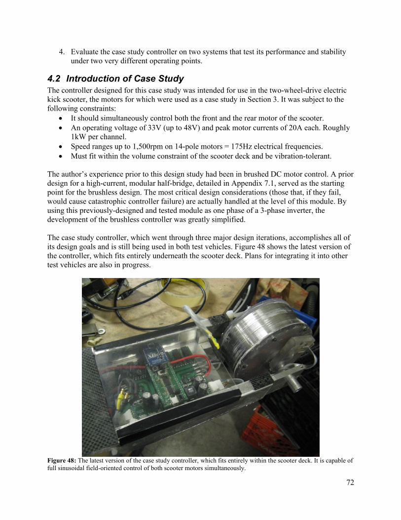
72

4. Evaluate the case study controller on two systems that test its performance and stability under two very different operating points.

4.2 Introduction of Case StudyThe controller designed for this case study was intended for use in the two-wheel-drive electric kick scooter, the motors for which were used as a case study in Section 3. It was subject to the following constraints:

It should simultaneously control both the front and the rear motor of the scooter. An operating voltage of 33V (up to 48V) and peak motor currents of 20A each. Roughly

1kW per channel. Speed ranges up to 1,500rpm on 14-pole motors = 175Hz electrical frequencies. Must fit within the volume constraint of the scooter deck and be vibration-tolerant.

The author’s experience prior to this design study had been in brushed DC motor control. A prior design for a high-current, modular half-bridge, detailed in Appendix 7.1, served as the starting point for the brushless design. The most critical design considerations (those that, if they fail, would cause catastrophic controller failure) are actually handled at the level of this module. By using this previously-designed and tested module as one phase of a 3-phase inverter, the development of the brushless controller was greatly simplified.

The case study controller, which went through three major design iterations, accomplishes all of its design goals and is still being used in both test vehicles. Figure 48 shows the latest version of the controller, which fits entirely underneath the scooter deck. Plans for integrating it into other test vehicles are also in progress.

Figure 48: The latest version of the case study controller, which fits entirely within the scooter deck. It is capable of full sinusoidal field-oriented control of both scooter motors simultaneously.

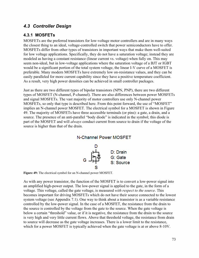
73

4.3 Controller Design

4.3.1 MOSFETsMOSFETs are the preferred transistors for low-voltage motor controllers and are in many ways the closest thing to an ideal, voltage-controlled switch that power semiconductors have to offer. MOSFETs differ from other types of transistors in important ways that make them well-suited for low voltage applications. Specifically, they do not have a saturation voltage; instead they are modeled as having a constant resistance (linear current vs. voltage) when fully on. This may seem non-ideal, but in low-voltage applications where the saturation voltage of a BJT or IGBT would be a significant portion of the total system voltage, the linear I-V curve of a MOSFET is preferable. Many modern MOSFETs have extremely low on-resistance values, and they can be easily paralleled for more current capability since they have a positive temperature coefficient. As a result, very high power densities can be achieved in small controller packages.

Just as there are two different types of bipolar transistors (NPN, PNP), there are two different types of MOSFET (N-channel, P-channel). There are also differences between power MOSFETs and signal MOSFETs. The vast majority of motor controllers use only N-channel power MOSFETs, so only that type is described here. From this point forward, the use of “MOSFET” implies an N-channel power MOSFET. The electrical symbol for a MOSFET is shown in Figure 49. The majority of MOSFETs have three accessible terminals (or pins): a gate, a drain, and a source. The presence of an anti-parallel “body diode” is indicated in the symbol; this diode is part of the MOSFET and will always conduct current from source to drain if the voltage of the source is higher than that of the drain.

Figure 49: The electrical symbol for an N-channel power MOSFET.

As with any power transistor, the function of the MOSFET is to convert a low-power signal into an amplified high-power output. The low-power signal is applied to the gate, in the form of a voltage. This voltage, called the gate voltage, is measured with respect to the source. This becomes important for driving MOSFETs which do not have their source connected to the lowest system voltage (see Appendix 7.1). One way to think about a transistor is as a variable resistance controlled by the low-power signal. In the case of a MOSFET, the resistance from the drain to the source is controlled by the voltage from the gate to the source. When the gate voltage is below a certain “threshold” value, or if it is negative, the resistance from the drain to the source is very high and very little current flows. Above that threshold voltage, the resistance from drain to source will decrease as the gate voltage increases. There is a lower limit to the resistance, which for a power MOSFET is typically achieved when the gate voltage is at or above 8-10V.

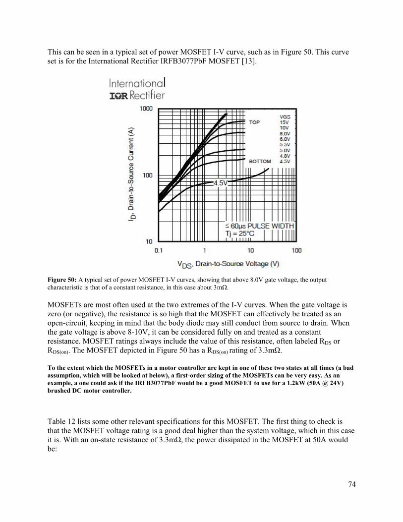
74

This can be seen in a typical set of power MOSFET I-V curve, such as in Figure 50. This curve set is for the International Rectifier IRFB3077PbF MOSFET [13].

Figure 50: A typical set of power MOSFET I-V curves, showing that above 8.0V gate voltage, the output characteristic is that of a constant resistance, in this case about 3mΩ.

MOSFETs are most often used at the two extremes of the I-V curves. When the gate voltage is zero (or negative), the resistance is so high that the MOSFET can effectively be treated as an open-circuit, keeping in mind that the body diode may still conduct from source to drain. When the gate voltage is above 8-10V, it can be considered fully on and treated as a constant resistance. MOSFET ratings always include the value of this resistance, often labeled RDS or RDS(on). The MOSFET depicted in Figure 50 has a RDS(on) rating of 3.3mΩ.

To the extent which the MOSFETs in a motor controller are kept in one of these two states at all times (a bad assumption, which will be looked at below), a first-order sizing of the MOSFETs can be very easy. As an example, a one could ask if the IRFB3077PbF would be a good MOSFET to use for a 1.2kW (50A @ 24V) brushed DC motor controller.

Table 12 lists some other relevant specifications for this MOSFET. The first thing to check is that the MOSFET voltage rating is a good deal higher than the system voltage, which in this case it is. With an on-state resistance of 3.3mΩ, the power dissipated in the MOSFET at 50A would be:

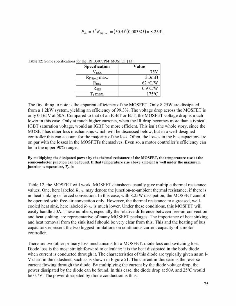
75

.25.80033.050 2)(

2 WARIP onDSdis

Table 12: Some specifications for the IRFB3077PbF MOSFET [13].

Specification ValueVDSS 75V

RDS(on) max. 3.3mΩRθJA 62 ºC/WRθJS 0.9ºC/W

TJ max. 175ºC

The first thing to note is the apparent efficiency of the MOSFET. Only 8.25W are dissipated from a 1.2kW system, yielding an efficiency of 99.3%. The voltage drop across the MOSFET is only 0.165V at 50A. Compared to that of an IGBT or BJT, the MOSFET voltage drop is much lower in this case. Only at much higher currents, when the IR drop becomes more than a typical IGBT saturation voltage, would an IGBT be more efficient. This isn’t the whole story, since the MOSET has other loss mechanisms which will be discussed below, but in a well-designed controller this can account for the majority of the loss. Often, the losses in the bus capacitors are on par with the losses in the MOSFETs themselves. Even so, a motor controller’s efficiency can be in the upper 90% range.

By multiplying the dissipated power by the thermal resistance of the MOSFET, the temperature rise at the semiconductor junction can be found. If that temperature rise above ambient is well under the maximum junction temperature, TJ, in

Table 12, the MOSFET will work. MOSFET datasheets usually give multiple thermal resistance values. One, here labeled RθJA, may denote the junction-to-ambient thermal resistance, if there is no heat sinking or forced convection. In this case, with 8.25W dissipation, the MOSFET cannot be operated with free-air convection only. However, the thermal resistance to a greased, well-cooled heat sink, here labeled RθJS, is much lower. Under these conditions, this MOSFET will easily handle 50A. These numbers, especially the relative difference between free-air convection and heat sinking, are representative of many MOSFET packages. The importance of heat sinking and heat removal from the sink itself should be very clear from this. This and the heating of bus capacitors represent the two biggest limitations on continuous current capacity of a motor controller.

There are two other primary loss mechanisms for a MOSFET: diode loss and switching loss. Diode loss is the most straightforward to calculate: it is the heat dissipated in the body diode when current is conducted through it. The characteristics of this diode are typically given as an I-V chart in the datasheet, such as is shown in Figure 51. The current in this case is the reverse current flowing through the diode. By multiplying the current by the diode voltage drop, the power dissipated by the diode can be found. In this case, the diode drop at 50A and 25ºC would be 0.7V. The power dissipated by diode conduction is thus:

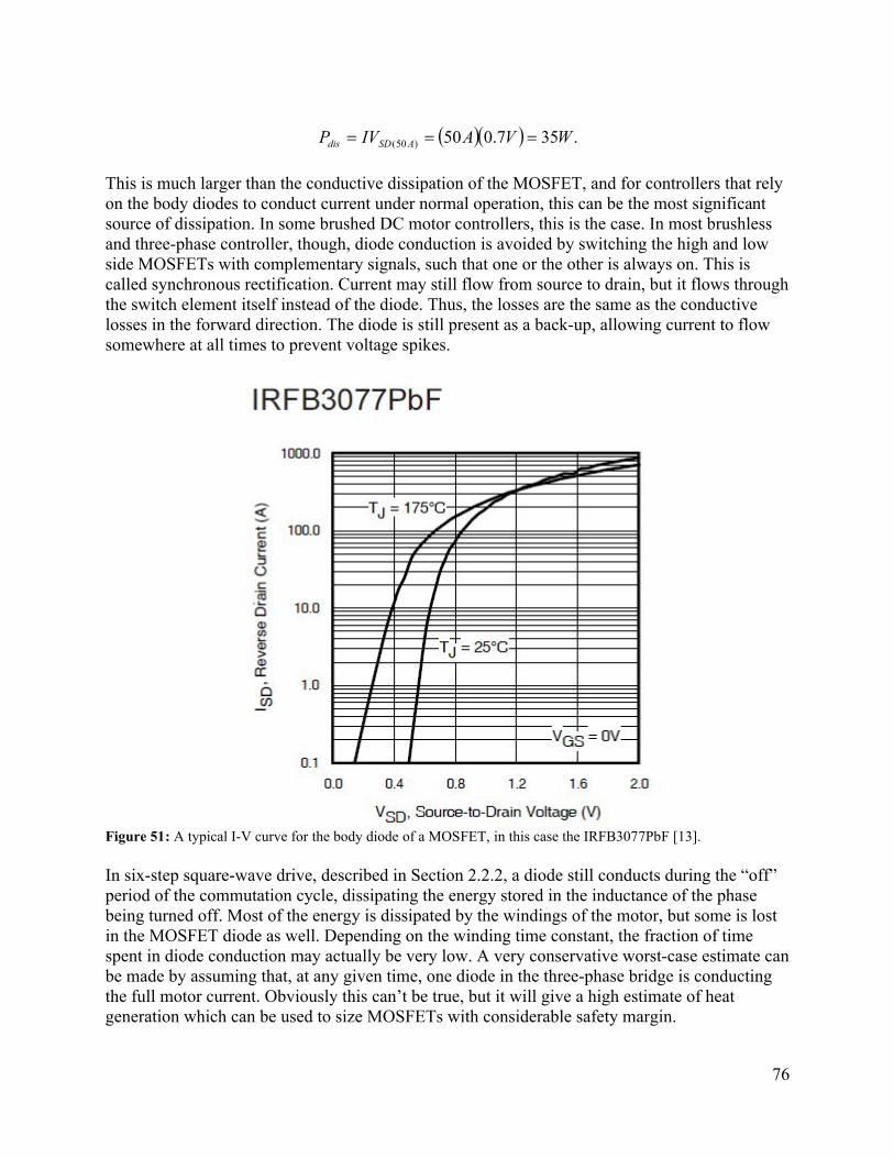
76

.357.050)50( WVAIVP ASDdis

This is much larger than the conductive dissipation of the MOSFET, and for controllers that rely on the body diodes to conduct current under normal operation, this can be the most significant source of dissipation. In some brushed DC motor controllers, this is the case. In most brushless and three-phase controller, though, diode conduction is avoided by switching the high and low side MOSFETs with complementary signals, such that one or the other is always on. This is called synchronous rectification. Current may still flow from source to drain, but it flows through the switch element itself instead of the diode. Thus, the losses are the same as the conductive losses in the forward direction. The diode is still present as a back-up, allowing current to flow somewhere at all times to prevent voltage spikes.

Figure 51: A typical I-V curve for the body diode of a MOSFET, in this case the IRFB3077PbF [13].

In six-step square-wave drive, described in Section 2.2.2, a diode still conducts during the “off” period of the commutation cycle, dissipating the energy stored in the inductance of the phase being turned off. Most of the energy is dissipated by the windings of the motor, but some is lost in the MOSFET diode as well. Depending on the winding time constant, the fraction of time spent in diode conduction may actually be very low. A very conservative worst-case estimate can be made by assuming that, at any given time, one diode in the three-phase bridge is conducting the full motor current. Obviously this can’t be true, but it will give a high estimate of heat generation which can be used to size MOSFETs with considerable safety margin.

77

In sine-wave drive, three MOSFETs are on at any given time (synchronous rectification of each half-bridge) and diode conduction is rarely required. Thus, diode losses are minimal. Only during faults, brief dead times, and other short-duration events do the diodes conduct. However, it may still be appropriate to size the MOSFETs such that one continuous diode loss can be tolerated, for a large margin of safety.

Switching loss is the last and more difficult to analyze MOSFET loss mechanism. This is the loss that occurs as a result of the fact that the MOSFET cannot be turned on or off instantaneously. The MOSFET gate has a small but important capacitance, modeled as in Figure 52, which creates a low-pass filter with the external gate resistor, slowing down the turn-on and turn-off transitions. As it transitions between having a very large resistance while off to having its on-state resistance, it passes through intermediate resistance values that dissipate much more power than either extreme. Because the resistance from drain to source is a nonlinear function of the gate voltage, it is hard to analytically estimate the switching losses with no point of reference. A brute-force approach to the analysis might be to integrate the instantaneous power loss along the path the MOSFET takes through an I-V curve as the gate is charged. Simulation is the most effective method for predicting switching losses, as tools like SPICE have extensive MOSFET models that accounts for the exact shape of the I-V curve. Since the goal of this analysis is to size the MOSFET with a large safety margin, a simple worst-case method is presented instead.

Figure 52: The effective internal capacitance from the gate to the source causes finite turn-on and turn-off time.

Though the path through the I-V curve during a switching event is unknown, the most extreme case would be that during a switching transient, the MOSFET has both the maximum voltage across it and the maximum current flowing through it at the same time. This means that for the entire duration of the turn-on or turn-off time, it takes on the worst possible resistance value: the one that dissipates the most power. The maximum voltage is simply the full DC voltage of the motor controller power supply. The maximum current could have many meanings. For extreme robustness, this could be the motor stall current. In most cases, it is the expected maximum operating current, which is much less than the stall current.

Another way of looking at it is that, in the worst-case scenario, all of the power is going into heating of the MOSFET during a switching transient. This should reveal the importance of a robust gate driver: If the MOSFET were somehow to get stuck in the half-on state, the failure would be catastrophic. This is probably the most dramatic, fastest, and in many cases most common failure mode of MOSFETs.

78

By keeping the switching transients very short compared to the time between them, the average power dissipation during switching can be kept low. The time of a switching transient is the time it takes the gate to get from 0V to the fully-on voltage (10V) or to get from 10V to 0V. Because gate drives have a limited current output, a gate resistor is used to keep the current applied in a reasonable range. This, with the gate capacitance, determines a time constant that governs the voltage rise or fall on the gate. If a 15V gate drive is used, the time to get to 10V is approximately one time constant (63% of 15V is 9.45V). A significant overestimate of the energy dissipated during one turn-on or turn-off event can be calculated, then as follows:

GGdis CRVIE maxmax ,

where RG is the gate resistor used in series with the gate driver and CG is the effective gate capacitance, often listed on the MOSFET datasheet as the “input capacitance.” The power dissipated is this energy multiplied by the number of turn-on and turn-off events per second, or twice the switching frequency:

GGswdisswdis CRVIfEfP maxmax22 .

Using the maximum current and voltage of the example 1.2kW DC motor drive, as well as the published CG of the IRFB3077PbF MOSFET (9.4nF), a 10Ω gate resistance (~1.5A gate driver current), and a 16kHz switching frequency, the power dissipated through switching is 3.61W. Even with this worst-case scenario analysis, the switching dissipation is less than the conductive dissipation and much less than the diode dissipation. In a well-designed motor controller, this should be the case. However, in many instances the time constant of the gate resistor and capacitance is too long or the switching frequency too high, resulting in larger switching losses.

The only thing intrinsic to the MOSFET itself that affects switching losses are the shape of the I-V curve as a function of gate voltage, and the gate capacitance. As far as the worst-case analysis goes, only the gate capacitance matters. The smaller the gate capacitance, the faster a MOSFET will turn on and off with a given gate driver, which will result in lower switching losses. Sometimes, the MOSFET datasheet will list a gate charge, in Coulombs, instead of a gate (input) capacitance. In this case, the gate voltage will usually be specified as well, and the gate capacitance can be calculated by:

.GS

GG V

QC

In other cases, a MOSFET datasheet may explicitly define a switching energy dissipation at a given set of operating conditions (a gate voltage and resistance, as well as the operating voltage and current across the switch, are the necessary parameters). In this case, the switching losses can be found by scaling this value appropriately, with the following considerations in mind:

Switching losses in a MOSFET will be the switching energy loss scaled by twice the switching frequency, to account for turn-on and turn-off time.

Switching energy loss will scale proportionally with switched current.

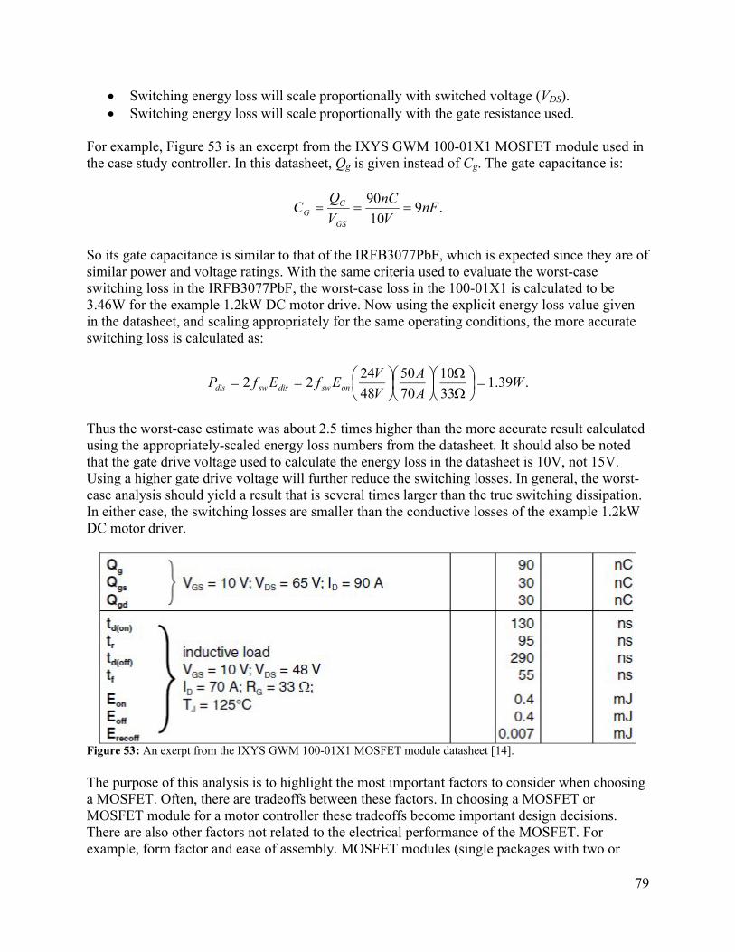
79

Switching energy loss will scale proportionally with switched voltage (VDS). Switching energy loss will scale proportionally with the gate resistance used.

For example, Figure 53 is an excerpt from the IXYS GWM 100-01X1 MOSFET module used in the case study controller. In this datasheet, Qg is given instead of Cg. The gate capacitance is:

.910

90nF

V

nC

V

QC

GS

GG

So its gate capacitance is similar to that of the IRFB3077PbF, which is expected since they are of similar power and voltage ratings. With the same criteria used to evaluate the worst-case switching loss in the IRFB3077PbF, the worst-case loss in the 100-01X1 is calculated to be 3.46W for the example 1.2kW DC motor drive. Now using the explicit energy loss value given in the datasheet, and scaling appropriately for the same operating conditions, the more accurate switching loss is calculated as:

.39.133

10

70

50

48

2422 W

A

A

V

VEfEfP onswdisswdis

Thus the worst-case estimate was about 2.5 times higher than the more accurate result calculated using the appropriately-scaled energy loss numbers from the datasheet. It should also be noted that the gate drive voltage used to calculate the energy loss in the datasheet is 10V, not 15V. Using a higher gate drive voltage will further reduce the switching losses. In general, the worst-case analysis should yield a result that is several times larger than the true switching dissipation. In either case, the switching losses are smaller than the conductive losses of the example 1.2kW DC motor driver.

Figure 53: An exerpt from the IXYS GWM 100-01X1 MOSFET module datasheet [14].

The purpose of this analysis is to highlight the most important factors to consider when choosing a MOSFET. Often, there are tradeoffs between these factors. In choosing a MOSFET or MOSFET module for a motor controller these tradeoffs become important design decisions. There are also other factors not related to the electrical performance of the MOSFET. For example, form factor and ease of assembly. MOSFET modules (single packages with two or

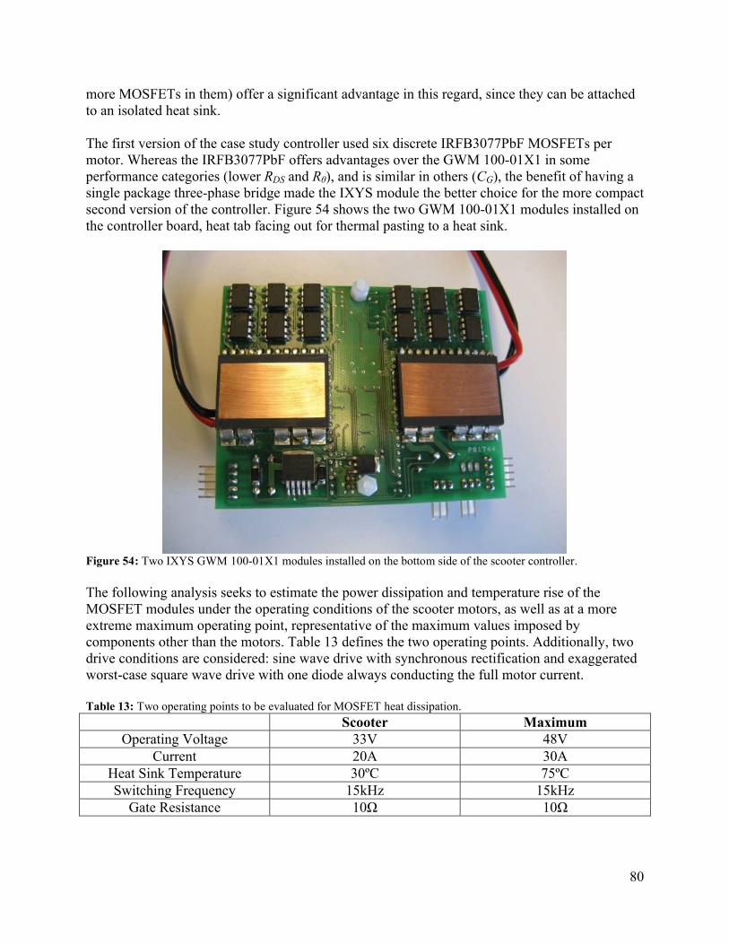
80

more MOSFETs in them) offer a significant advantage in this regard, since they can be attached to an isolated heat sink.

The first version of the case study controller used six discrete IRFB3077PbF MOSFETs per motor. Whereas the IRFB3077PbF offers advantages over the GWM 100-01X1 in some performance categories (lower RDS and Rθ), and is similar in others (CG), the benefit of having a single package three-phase bridge made the IXYS module the better choice for the more compact second version of the controller. Figure 54 shows the two GWM 100-01X1 modules installed on the controller board, heat tab facing out for thermal pasting to a heat sink.

Figure 54: Two IXYS GWM 100-01X1 modules installed on the bottom side of the scooter controller.

The following analysis seeks to estimate the power dissipation and temperature rise of the MOSFET modules under the operating conditions of the scooter motors, as well as at a more extreme maximum operating point, representative of the maximum values imposed by components other than the motors. Table 13 defines the two operating points. Additionally, two drive conditions are considered: sine wave drive with synchronous rectification and exaggerated worst-case square wave drive with one diode always conducting the full motor current.

Table 13: Two operating points to be evaluated for MOSFET heat dissipation.

Scooter MaximumOperating Voltage 33V 48V

Current 20A 30AHeat Sink Temperature 30ºC 75ºCSwitching Frequency 15kHz 15kHz

Gate Resistance 10Ω 10Ω

81

The first step is an estimate of the power dissipation by conductive losses. In square wave drive, only two MOSFETs in the bridge are conducting current at any given time. In sine wave drive, three are conducting at any one point, but the RMS current is the relevant parameter. For the purpose of this analysis, the RMS current will be set to the value listed in Table 13. Note that the two drives (square wave versus sine wave) will have different torque-speed outputs! The relevant equation is:

)(2

, onDSondis RnIP ,

where n is the number of MOSFET conducting, I is the current being considered, and RDS(on) is the on-resistance of a single MOSFET. Since the RDS(on) value is a function of temperature, a worst-case estimate is taken using the value at TJ=125ºC. Table 14 shows the calculation of conductive dissipation for the four cases being considered.

Table 14: The conductive dissipation, Pdis,on, for the four cases being considered.

Scooter, Square-Wave Drive

WmAP ondis 65.7202 2,

Maximum, Square Wave Drive

WmAP ondis 2.2514302 2,

Scooter, Sine Wave Drive

WmAP ondis 95.7203 2,

Maximum, Sine Wave Drive

WmAP ondis 8.3714303 2,

Next, the diode dissipation is considered for all four cases. In both sine wave drive cases, the diode dissipation is negligible. In square wave drive, an exaggerated worst-case estimate can be made by assuming one diode (either the high side or low side) in the “off” phase leg is conducting the full motor current at any given time. The diode I-V characteristic at different junction temperatures is given in the GWM 100-01X1 datasheet. The equation used to calculate diode dissipation is:

,, SDddis IVP

where I the current being considered and VSD is the diode voltage drop, given by the MOSFET data sheet for different values of diode current. Table 15 shows the calculation of diode dissipation for all four cases.

Table 15: The diode dissipation, Pdis,d, for the four cases beind considered.

Scooter, Square Wave Drive WVAP ddis 168.020,

Maximum, Square Wave Drive WVAP ddis 6.2482.030,

Scooter, Sine Wave DriveWP ddis 0,

Maximum, Sine Wave DriveWP ddis 0,

Finally, switching losses are considered. By appropriately scaling the given energy dissipation per switching transient to the operating conditions under consideration, an estimate of the switching loss power can be made:

33

10

70484.01522, A

I

V

VmJkHznEnfP disswswdis ,

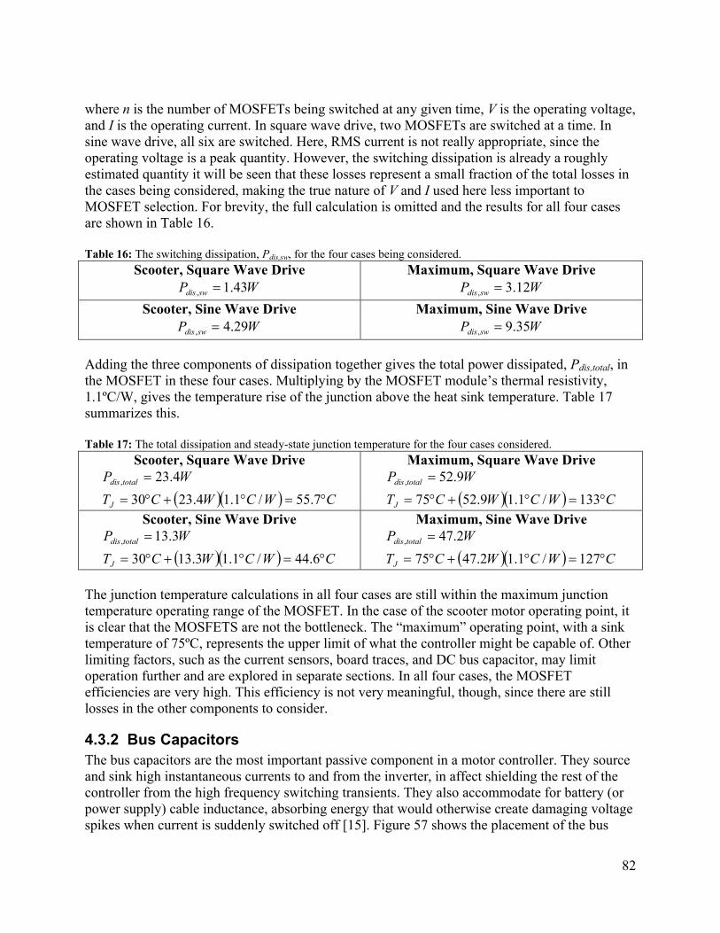
82

where n is the number of MOSFETs being switched at any given time, V is the operating voltage, and I is the operating current. In square wave drive, two MOSFETs are switched at a time. In sine wave drive, all six are switched. Here, RMS current is not really appropriate, since the operating voltage is a peak quantity. However, the switching dissipation is already a roughly estimated quantity it will be seen that these losses represent a small fraction of the total losses in the cases being considered, making the true nature of V and I used here less important to MOSFET selection. For brevity, the full calculation is omitted and the results for all four cases are shown in Table 16.

Table 16: The switching dissipation, Pdis,sw, for the four cases being considered.

Scooter, Square Wave DriveWP swdis 43.1,

Maximum, Square Wave DriveWP swdis 12.3,

Scooter, Sine Wave DriveWP swdis 29.4,

Maximum, Sine Wave DriveWP swdis 35.9,

Adding the three components of dissipation together gives the total power dissipated, Pdis,total, in the MOSFET in these four cases. Multiplying by the MOSFET module’s thermal resistivity, 1.1ºC/W, gives the temperature rise of the junction above the heat sink temperature. Table 17summarizes this.

Table 17: The total dissipation and steady-state junction temperature for the four cases considered.

Scooter, Square Wave Drive

CWCWCT

WP

J

totaldis

7.55/1.14.2330

4.23,

Maximum, Square Wave Drive

CWCWCT

WP

J

totaldis

133/1.19.5275

9.52,

Scooter, Sine Wave Drive

CWCWCT

WP

J

totaldis

6.44/1.13.1330

3.13,

Maximum, Sine Wave Drive

CWCWCT

WP

J

totaldis

127/1.12.4775

2.47,

The junction temperature calculations in all four cases are still within the maximum junction temperature operating range of the MOSFET. In the case of the scooter motor operating point, it is clear that the MOSFETS are not the bottleneck. The “maximum” operating point, with a sink temperature of 75ºC, represents the upper limit of what the controller might be capable of. Other limiting factors, such as the current sensors, board traces, and DC bus capacitor, may limit operation further and are explored in separate sections. In all four cases, the MOSFET efficiencies are very high. This efficiency is not very meaningful, though, since there are still losses in the other components to consider.

4.3.2 Bus CapacitorsThe bus capacitors are the most important passive component in a motor controller. They source and sink high instantaneous currents to and from the inverter, in affect shielding the rest of the controller from the high frequency switching transients. They also accommodate for battery (or power supply) cable inductance, absorbing energy that would otherwise create damaging voltage spikes when current is suddenly switched off [15]. Figure 57 shows the placement of the bus

83

capacitor; it is crucial that the capacitor be physically located as close as possible to the inverter MOSFETs, so that the resistance and inductance of the line between the capacitor and the MOSFETs is very low. Figure 59 shows the physical placement of the bus capacitors in this controller. Each inverter gets a separate bus capacitor, located immediately adjacent to the MOSFET module’s power terminals.

Figure 55: The bus capacitor is placed across the DC lines, as close as possible to the inverter MOSFETs.

The bus capacitor is typically an electrolytic capacitor, or a group of electrolytic capacitors in parallel. In high-current controllers, it can occupy as much or more volume than the MOSFETs themselves. It can also dissipate as much or more heat, meaning it contributes significantly to the overall efficiency of the controller. Sizing the bus capacitor is critical to a motor controller design. There are two main considerations for sizing: voltage ripple and heating.

Voltage ripple is easy to predict by making the worst-case assumption that the bus capacitor supplies all of the switching current at the PWM frequency. In this case, the power supply provides only a steady DC current. When the PWM is off, the bus capacitor is charged by the power supply current. When the PWM is on, the bus capacitor is discharged, sourcing current (in addition to the power supply current) to the MOSFETs. Table 18 lists the currents present in these two states.

Table 18: Current flow during the PWM on and off times, assuming the power supply provides only a DC average current (high power supply inductance and/or high frequency).

Power Supply Current MOSFET Current Capacitor CurrentPWM Off (1-D) (D)Imotor 0 (D)Imotor

PWM On (D) (D)Imotor Imotor -(1-D)Imotor

The duty cycle, D, is the fraction of time the PWM is on. (1-D) is t off time. By taking the time-weighted sum of the currents in Table 18, the average current in from the power supply over one switching cycle is the same as the average current out to the MOSFET. Additionally, the average capacitor current is zero, a necessary condition for steady-state.

The voltage ripple depends on the current, the duty cycle, and the switching frequency. Starting from the constitutive equation for a capacitor, it can be calculated as follows:

84

sw

motor

f

D

C

DIt

C

IV

C

I

dt

dV

1

This is the calculation for charging. Discharging will yield the same equation, but with a negative change in voltage. (So that over one switching cycle in steady-state, the capacitor returns to the same voltage.) From this, it is easy to see that the maximum ripple voltage occurs at 50% duty cycle, where D(1-D) = 0.25.

The capacitors for each inverter in the case study controller are 330μF, 63V electrolytic capacitors. The switching frequency is 14.5kHz. The peak motor current is 30A. Carrying out the voltage ripple calculation with these values yields ΔV = 1.57V at 50% duty cycle. This would not make a very good switching power supply, but for a motor controller it is acceptable. The important criterion is that the voltage does not exceed any hard limits (such as MOSFET breakdown voltage or power supply low voltage cutoff). For the RC car, which has peak currents of 40A and a voltage supply that is only 1.8V higher than the cutoff, a set of two 560μF/35V capacitors is used instead. In general, the lower the system voltage, the higher capacitance is available in the same form factor.

The other important design consideration in sizing the bus capacitor is heat generation. Calculating the capacitor heat loss is impossible without knowing the ripple current more exactly. The worst-case assumption, though, is the same as in the voltage ripple calculation: the bus capacitor supplies the entire AC component of current, at 50% duty cycle. One way to very roughly estimate capacitor heating is using the “loss tangent,” which is defined as follows:

CR tan .

The value tan δ is often published in capacitor datasheets, and is assumed to be constant for all frequencies ω. C is the capacitance and R is an equivalent series resistance. From this, it is clear that that equivalent series resistance decreases with increasing frequency. Using tan δ = 0.1, from the datasheet for the capacitors in this controller, the equivalent series resistance at 14.5kHz is:

mFkHzC

R 3.33305.142

1.0tan

.

This is likely a low estimate of the equivalent series resistance, since in reality the assumption that tan δ = constant does not hold true at high frequency. Instead, the equivalent resistance settles out to some minimum value. The crossover is typically below 10kHz [16]. The full curve is not usually published in capacitor datasheet. Knowing that the resistance value predicted by the low tangent is a low estimate is still useful. The order of magnitude starting here and going up (to 33mΩ in this case) can be analyzed. Figure 56 shows a plot over this range of resistances of capacitor heat generation with a motor current of 30A and 50% duty cycle (15A in/out).

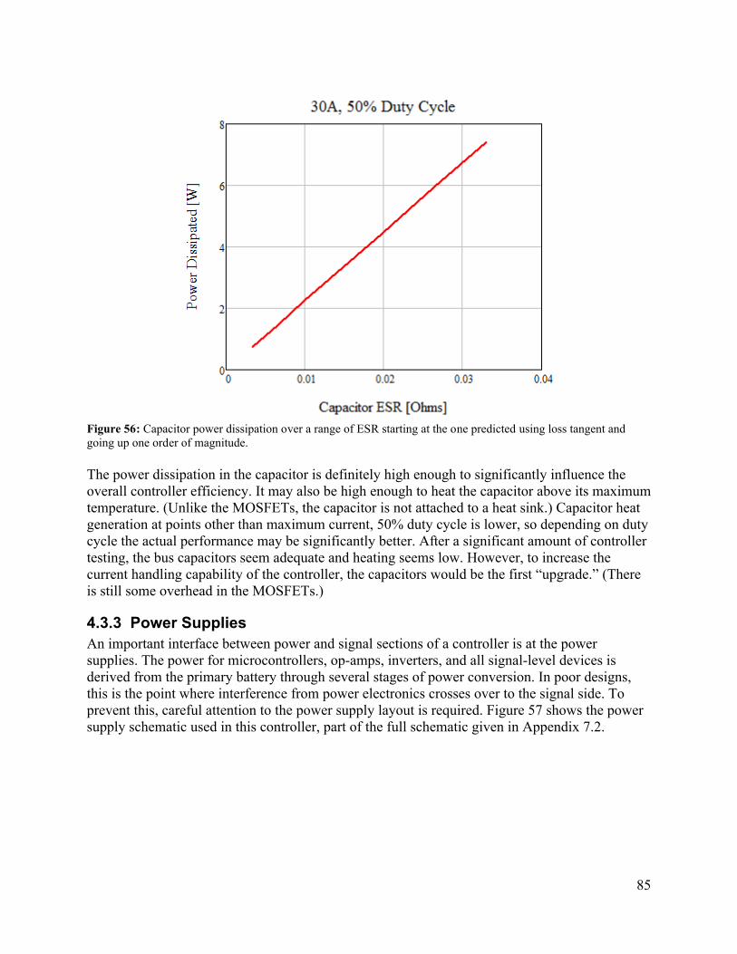
85

Figure 56: Capacitor power dissipation over a range of ESR starting at the one predicted using loss tangent and going up one order of magnitude.

The power dissipation in the capacitor is definitely high enough to significantly influence the overall controller efficiency. It may also be high enough to heat the capacitor above its maximum temperature. (Unlike the MOSFETs, the capacitor is not attached to a heat sink.) Capacitor heat generation at points other than maximum current, 50% duty cycle is lower, so depending on duty cycle the actual performance may be significantly better. After a significant amount of controller testing, the bus capacitors seem adequate and heating seems low. However, to increase the current handling capability of the controller, the capacitors would be the first “upgrade.” (There is still some overhead in the MOSFETs.)

4.3.3 Power SuppliesAn important interface between power and signal sections of a controller is at the power supplies. The power for microcontrollers, op-amps, inverters, and all signal-level devices is derived from the primary battery through several stages of power conversion. In poor designs, this is the point where interference from power electronics crosses over to the signal side. To prevent this, careful attention to the power supply layout is required. Figure 57 shows the power supply schematic used in this controller, part of the full schematic given in Appendix 7.2.

86

Figure 57: The controller power supplies, an excerpt from the full schematic given in Appendix 7.2.

The first power supply is an efficient switching regulator, which converts battery voltage (24-48V) to 15V. The regulator used is made by National Semiconductor, part number LM2575HV. The “HV” stands for high voltage. This version can take up to a 63V input. The non-HV version can take a maximum input of 45V. Because it is a switching regulator, the LM2575HV requires an external diode (D7) and inductor (L1) to operate. It also requires a capacitor (C11) to smooth the output.

The switching regulator has its own bypass capacitor, C1, placed as close as possible to its inputs. This capacitor isolates the power supply from noise created by the inverters. Power from the battery, labeled V+, passes through a Shottky diode, D1, before even reaching the power supply input capacitor. This prevents current from flowing back from C1 to the positive DC bus, further isolating the power supplies from sudden increases in load on the inverters.

The 15V supply is used for powering the gate drivers. Thus, it is technically still on the “power” side of the circuit, susceptible to noise from the inverters. It can be further isolated from inverter noise by using the fully isolated half bridge layout, shown in 7.1.5. However, in this controller the 15V supply directly powers the low-side gate drivers, and the 15V supply is still susceptible to inverter noise.

The output of the 15V supply is also used to create the signal-level power supply (5V). A common linear regulator (7805, made by several manufacturers) is used to do this step-down. Linear regulator produce a clean output (no switching), which is good for signal electronics. However, they dissipate a lot more heat than switching regulators. The full voltage drop at operating current is dissipated. Thus, at just 0.1A of current, the 7805 regulator here would be dissipating 1W. It is only required to power signal-level components, so the current draw is small, but heat dissipation is still an important consideration. The surface mount component is directly soldered to the signal ground plane, which can help with heat sinking.

The ground connection between the 15V power supply and the 7805 is the only place where signal and power grounds connect. This single-point connection is very important, as will be discussed in Section 4.4.1. At the output of the 7805 linear regulator are two 1uF ceramic capacitors for additional smoothing. These values could certainly be increased. All components

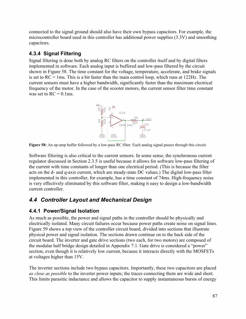
87

connected to the signal ground should also have their own bypass capacitors. For example, the microcontroller board used in this controller has additional power supplies (3.3V) and smoothing capacitors.

4.3.4 Signal FilteringSignal filtering is done both by analog RC filters on the controller itself and by digital filters implemented in software. Each analog input is buffered and low-pass filtered by the circuit shown in Figure 58. The time constant for the voltage, temperature, accelerate, and brake signals is set to RC = 1ms. This is a bit faster than the main control loop, which runs at 122Hz. The current sensors must have a higher bandwidth, significantly faster than the maximum electrical frequency of the motor. In the case of the scooter motors, the current sensor filter time constant was set to RC = 0.1ms.

Figure 58: An op-amp buffer followed by a low-pass RC filter. Each analog signal passes through this circuit.

Software filtering is also critical to the current sensors. In some sense, the synchronous current regulator discussed in Section 2.3.5 is useful because it allows for software low-pass filtering of the current with time constants of longer than one electrical period. (This is because the filter acts on the d- and q-axis current, which are steady-state DC values.) The digital low-pass filter implemented in this controller, for example, has a time constant of 74ms. High-frequency noise is very effectively eliminated by this software filter, making it easy to design a low-bandwidth current controller.

4.4 Controller Layout and Mechanical Design

4.4.1 Power/Signal IsolationAs much as possible, the power and signal paths in the controller should be physically and electrically isolated. Many circuit failures occur because power paths create noise on signal lines. Figure 59 shows a top view of the controller circuit board, divided into sections that illustrate physical power and signal isolation. The sections drawn continue on to the back side of the circuit board. The inverter and gate drive sections (two each, for two motors) are composed of the modular half bridge design detailed in Appendix 7.1. Gate drive is considered a “power” section, even though it is relatively low current, because it interacts directly with the MOSFETs at voltages higher than 15V.

The inverter sections include two bypass capacitors. Importantly, these two capacitors are placed as close as possible to the inverter power inputs; the traces connecting them are wide and short. This limits parasitic inductance and allows the capacitor to supply instantaneous bursts of energy

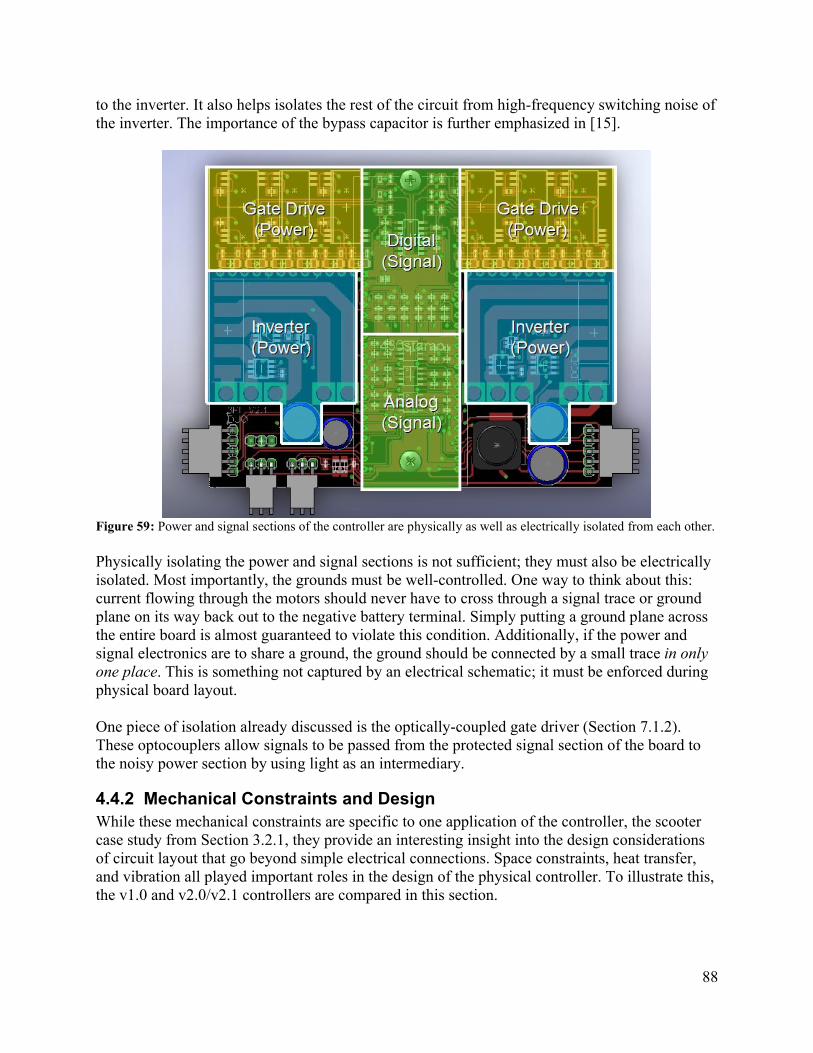
88

to the inverter. It also helps isolates the rest of the circuit from high-frequency switching noise of the inverter. The importance of the bypass capacitor is further emphasized in [15].

Figure 59: Power and signal sections of the controller are physically as well as electrically isolated from each other.

Physically isolating the power and signal sections is not sufficient; they must also be electrically isolated. Most importantly, the grounds must be well-controlled. One way to think about this: current flowing through the motors should never have to cross through a signal trace or ground plane on its way back out to the negative battery terminal. Simply putting a ground plane across the entire board is almost guaranteed to violate this condition. Additionally, if the power and signal electronics are to share a ground, the ground should be connected by a small trace in only one place. This is something not captured by an electrical schematic; it must be enforced during physical board layout.

One piece of isolation already discussed is the optically-coupled gate driver (Section 7.1.2). These optocouplers allow signals to be passed from the protected signal section of the board to the noisy power section by using light as an intermediary.

4.4.2 Mechanical Constraints and DesignWhile these mechanical constraints are specific to one application of the controller, the scooter case study from Section 3.2.1, they provide an interesting insight into the design considerations of circuit layout that go beyond simple electrical connections. Space constraints, heat transfer, and vibration all played important roles in the design of the physical controller. To illustrate this, the v1.0 and v2.0/v2.1 controllers are compared in this section.

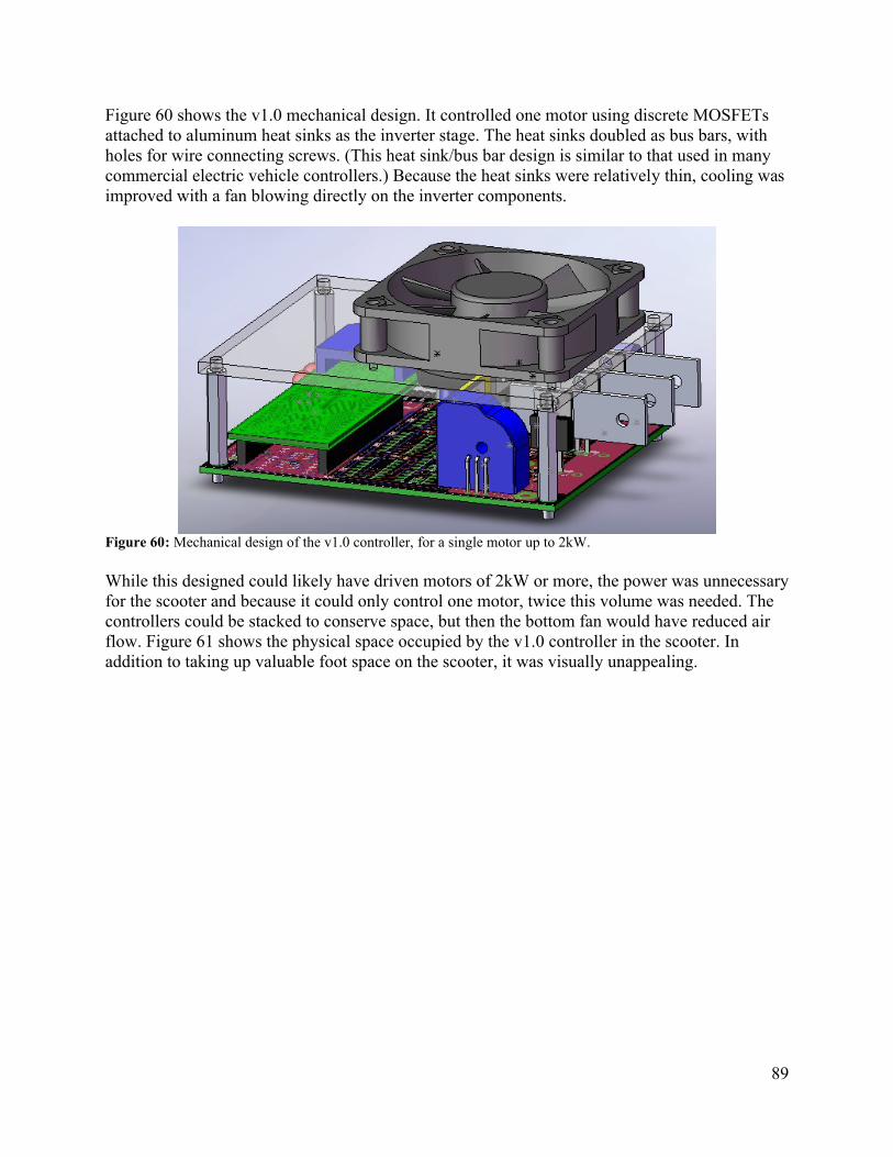
89

Figure 60 shows the v1.0 mechanical design. It controlled one motor using discrete MOSFETs attached to aluminum heat sinks as the inverter stage. The heat sinks doubled as bus bars, with holes for wire connecting screws. (This heat sink/bus bar design is similar to that used in many commercial electric vehicle controllers.) Because the heat sinks were relatively thin, cooling was improved with a fan blowing directly on the inverter components.

Figure 60: Mechanical design of the v1.0 controller, for a single motor up to 2kW.

While this designed could likely have driven motors of 2kW or more, the power was unnecessary for the scooter and because it could only control one motor, twice this volume was needed. The controllers could be stacked to conserve space, but then the bottom fan would have reduced air flow. Figure 61 shows the physical space occupied by the v1.0 controller in the scooter. In addition to taking up valuable foot space on the scooter, it was visually unappealing.

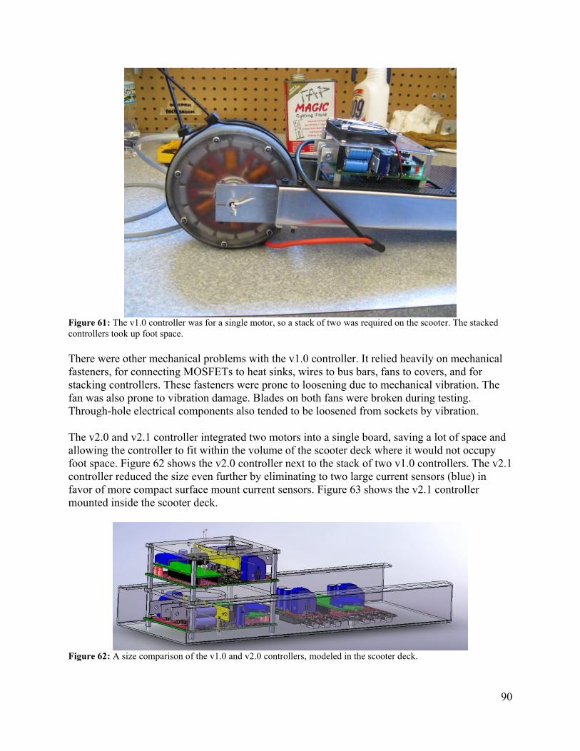
90

Figure 61: The v1.0 controller was for a single motor, so a stack of two was required on the scooter. The stacked controllers took up foot space.

There were other mechanical problems with the v1.0 controller. It relied heavily on mechanical fasteners, for connecting MOSFETs to heat sinks, wires to bus bars, fans to covers, and for stacking controllers. These fasteners were prone to loosening due to mechanical vibration. The fan was also prone to vibration damage. Blades on both fans were broken during testing. Through-hole electrical components also tended to be loosened from sockets by vibration.

The v2.0 and v2.1 controller integrated two motors into a single board, saving a lot of space and allowing the controller to fit within the volume of the scooter deck where it would not occupy foot space. Figure 62 shows the v2.0 controller next to the stack of two v1.0 controllers. The v2.1 controller reduced the size even further by eliminating to two large current sensors (blue) in favor of more compact surface mount current sensors. Figure 63 shows the v2.1 controller mounted inside the scooter deck.

Figure 62: A size comparison of the v1.0 and v2.0 controllers, modeled in the scooter deck.

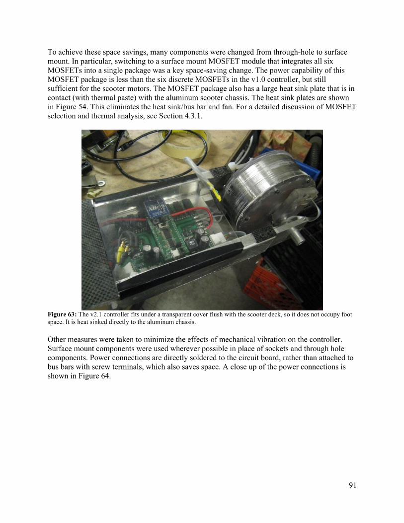
91

To achieve these space savings, many components were changed from through-hole to surface mount. In particular, switching to a surface mount MOSFET module that integrates all six MOSFETs into a single package was a key space-saving change. The power capability of this MOSFET package is less than the six discrete MOSFETs in the v1.0 controller, but still sufficient for the scooter motors. The MOSFET package also has a large heat sink plate that is in contact (with thermal paste) with the aluminum scooter chassis. The heat sink plates are shown in Figure 54. This eliminates the heat sink/bus bar and fan. For a detailed discussion of MOSFET selection and thermal analysis, see Section 4.3.1.

Figure 63: The v2.1 controller fits under a transparent cover flush with the scooter deck, so it does not occupy foot space. It is heat sinked directly to the aluminum chassis.

Other measures were taken to minimize the effects of mechanical vibration on the controller. Surface mount components were used wherever possible in place of sockets and through hole components. Power connections are directly soldered to the circuit board, rather than attached to bus bars with screw terminals, which also saves space. A close up of the power connections is shown in Figure 64.

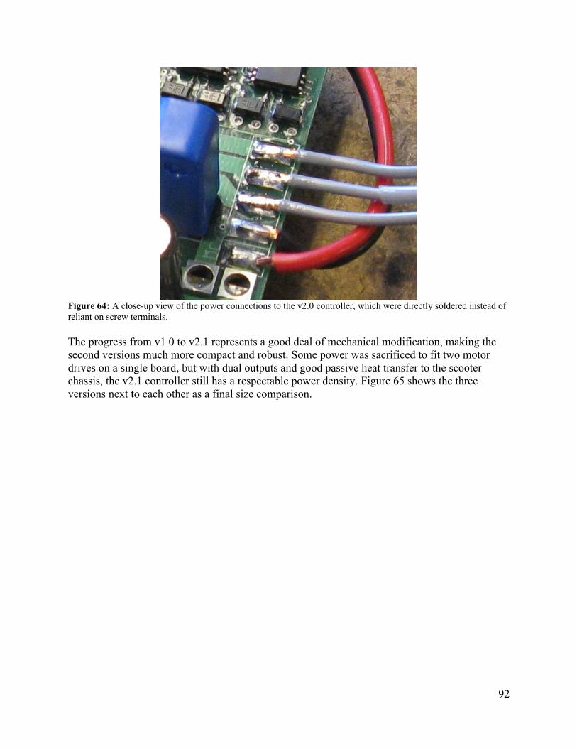
92

Figure 64: A close-up view of the power connections to the v2.0 controller, which were directly soldered instead of reliant on screw terminals.

The progress from v1.0 to v2.1 represents a good deal of mechanical modification, making the second versions much more compact and robust. Some power was sacrificed to fit two motor drives on a single board, but with dual outputs and good passive heat transfer to the scooter chassis, the v2.1 controller still has a respectable power density. Figure 65 shows the three versions next to each other as a final size comparison.

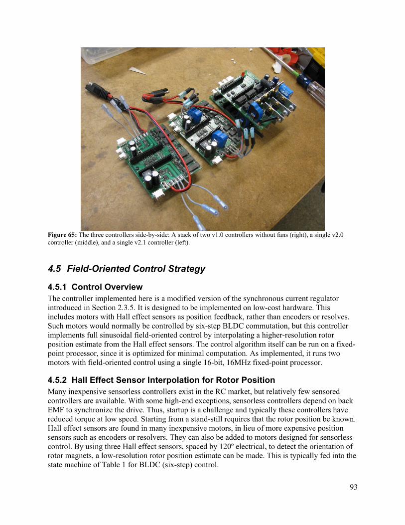
93

Figure 65: The three controllers side-by-side: A stack of two v1.0 controllers without fans (right), a single v2.0 controller (middle), and a single v2.1 controller (left).

4.5 Field-Oriented Control Strategy

4.5.1 Control OverviewThe controller implemented here is a modified version of the synchronous current regulator introduced in Section 2.3.5. It is designed to be implemented on low-cost hardware. This includes motors with Hall effect sensors as position feedback, rather than encoders or resolves. Such motors would normally be controlled by six-step BLDC commutation, but this controller implements full sinusoidal field-oriented control by interpolating a higher-resolution rotor position estimate from the Hall effect sensors. The control algorithm itself can be run on a fixed-point processor, since it is optimized for minimal computation. As implemented, it runs two motors with field-oriented control using a single 16-bit, 16MHz fixed-point processor.

4.5.2 Hall Effect Sensor Interpolation for Rotor PositionMany inexpensive sensorless controllers exist in the RC market, but relatively few sensored controllers are available. With some high-end exceptions, sensorless controllers depend on back EMF to synchronize the drive. Thus, startup is a challenge and typically these controllers have reduced torque at low speed. Starting from a stand-still requires that the rotor position be known. Hall effect sensors are found in many inexpensive motors, in lieu of more expensive position sensors such as encoders or resolvers. They can also be added to motors designed for sensorless control. By using three Hall effect sensors, spaced by 120º electrical, to detect the orientation of rotor magnets, a low-resolution rotor position estimate can be made. This is typically fed into the state machine of Table 1 for BLDC (six-step) control.

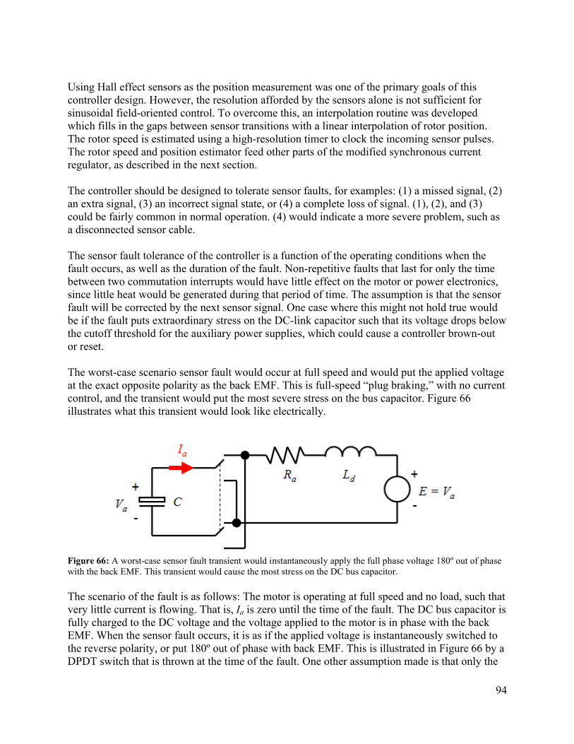
94

Using Hall effect sensors as the position measurement was one of the primary goals of this controller design. However, the resolution afforded by the sensors alone is not sufficient for sinusoidal field-oriented control. To overcome this, an interpolation routine was developed which fills in the gaps between sensor transitions with a linear interpolation of rotor position. The rotor speed is estimated using a high-resolution timer to clock the incoming sensor pulses. The rotor speed and position estimator feed other parts of the modified synchronous current regulator, as described in the next section.

The controller should be designed to tolerate sensor faults, for examples: (1) a missed signal, (2) an extra signal, (3) an incorrect signal state, or (4) a complete loss of signal. (1), (2), and (3) could be fairly common in normal operation. (4) would indicate a more severe problem, such as a disconnected sensor cable.

The sensor fault tolerance of the controller is a function of the operating conditions when the fault occurs, as well as the duration of the fault. Non-repetitive faults that last for only the time between two commutation interrupts would have little effect on the motor or power electronics, since little heat would be generated during that period of time. The assumption is that the sensor fault will be corrected by the next sensor signal. One case where this might not hold true would be if the fault puts extraordinary stress on the DC-link capacitor such that its voltage drops below the cutoff threshold for the auxiliary power supplies, which could cause a controller brown-out or reset.

The worst-case scenario sensor fault would occur at full speed and would put the applied voltage at the exact opposite polarity as the back EMF. This is full-speed “plug braking,” with no current control, and the transient would put the most severe stress on the bus capacitor. Figure 66illustrates what this transient would look like electrically.

Figure 66: A worst-case sensor fault transient would instantaneously apply the full phase voltage 180º out of phase with the back EMF. This transient would cause the most stress on the DC bus capacitor.

The scenario of the fault is as follows: The motor is operating at full speed and no load, such that very little current is flowing. That is, Ia is zero until the time of the fault. The DC bus capacitor is fully charged to the DC voltage and the voltage applied to the motor is in phase with the back EMF. When the sensor fault occurs, it is as if the applied voltage is instantaneously switched to the reverse polarity, or put 180º out of phase with back EMF. This is illustrated in Figure 66 by a DPDT switch that is thrown at the time of the fault. One other assumption made is that only the

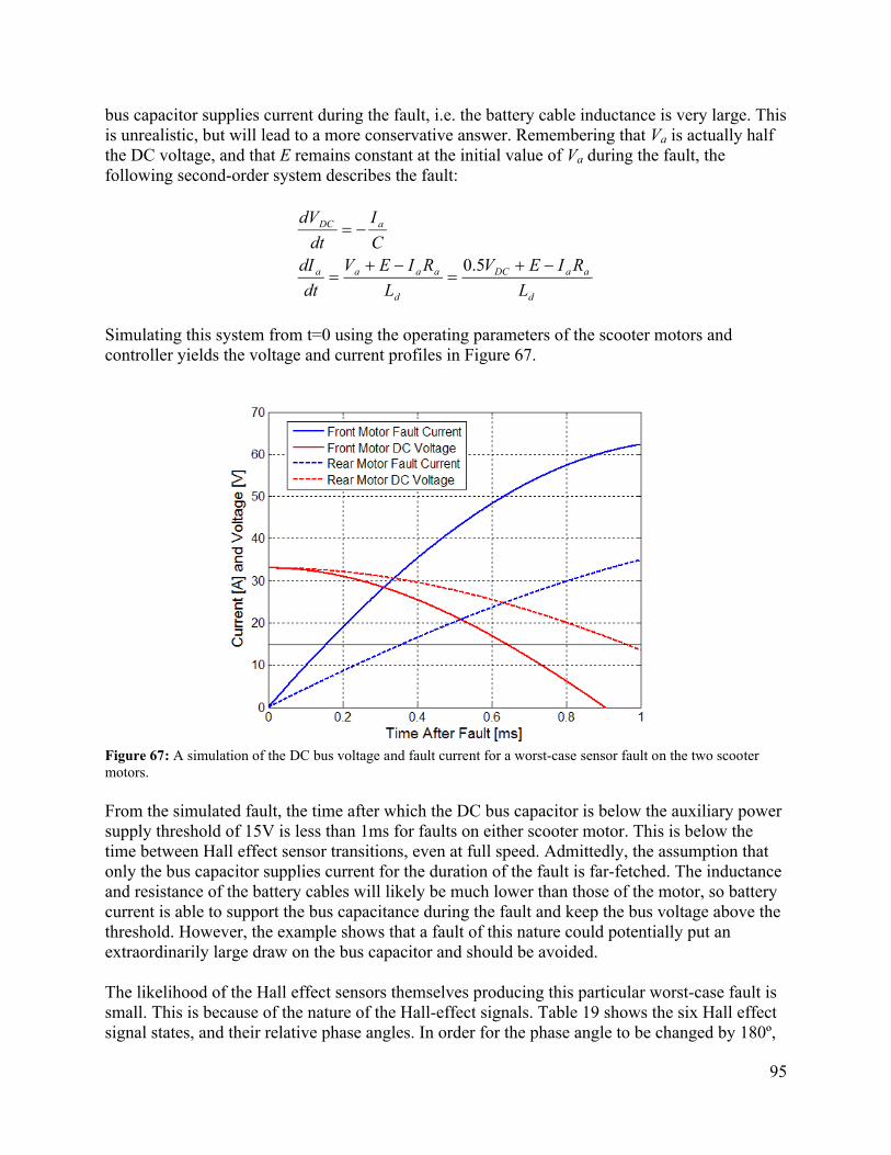
95

bus capacitor supplies current during the fault, i.e. the battery cable inductance is very large. This is unrealistic, but will lead to a more conservative answer. Remembering that Va is actually half the DC voltage, and that E remains constant at the initial value of Va during the fault, the following second-order system describes the fault:

d

aaDC

d

aaaa

aDC

L

RIEV

L

RIEV

dt

dIC

I

dt

dV

5.0

Simulating this system from t=0 using the operating parameters of the scooter motors and controller yields the voltage and current profiles in Figure 67.

Figure 67: A simulation of the DC bus voltage and fault current for a worst-case sensor fault on the two scooter motors.

From the simulated fault, the time after which the DC bus capacitor is below the auxiliary power supply threshold of 15V is less than 1ms for faults on either scooter motor. This is below the time between Hall effect sensor transitions, even at full speed. Admittedly, the assumption that only the bus capacitor supplies current for the duration of the fault is far-fetched. The inductance and resistance of the battery cables will likely be much lower than those of the motor, so battery current is able to support the bus capacitance during the fault and keep the bus voltage above the threshold. However, the example shows that a fault of this nature could potentially put an extraordinarily large draw on the bus capacitor and should be avoided.

The likelihood of the Hall effect sensors themselves producing this particular worst-case fault is small. This is because of the nature of the Hall-effect signals. Table 19 shows the six Hall effect signal states, and their relative phase angles. In order for the phase angle to be changed by 180º,

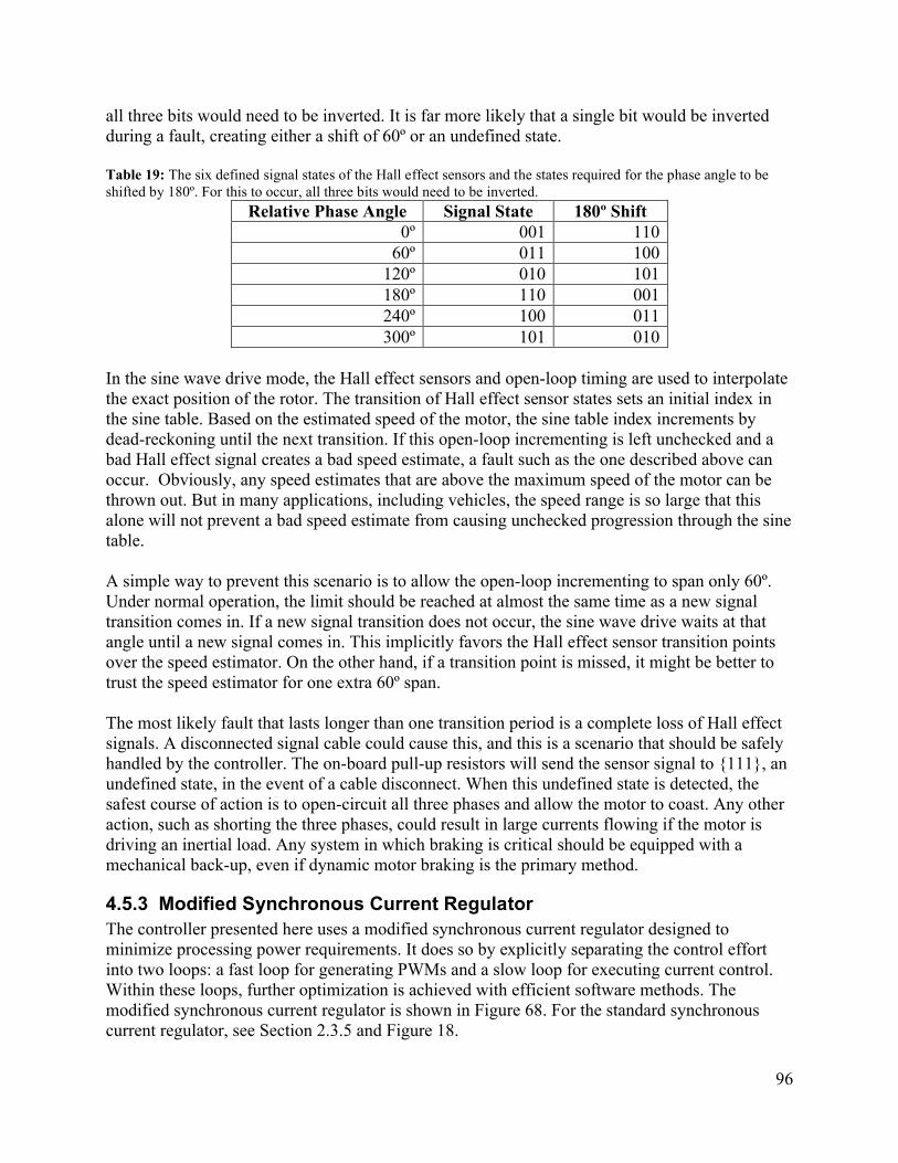
96

all three bits would need to be inverted. It is far more likely that a single bit would be inverted during a fault, creating either a shift of 60º or an undefined state.

Table 19: The six defined signal states of the Hall effect sensors and the states required for the phase angle to be shifted by 180º. For this to occur, all three bits would need to be inverted.

Relative Phase Angle Signal State 180º Shift0º 001 110

60º 011 100120º 010 101180º 110 001240º 100 011300º 101 010

In the sine wave drive mode, the Hall effect sensors and open-loop timing are used to interpolate the exact position of the rotor. The transition of Hall effect sensor states sets an initial index in the sine table. Based on the estimated speed of the motor, the sine table index increments by dead-reckoning until the next transition. If this open-loop incrementing is left unchecked and a bad Hall effect signal creates a bad speed estimate, a fault such as the one described above can occur. Obviously, any speed estimates that are above the maximum speed of the motor can be thrown out. But in many applications, including vehicles, the speed range is so large that this alone will not prevent a bad speed estimate from causing unchecked progression through the sine table.

A simple way to prevent this scenario is to allow the open-loop incrementing to span only 60º. Under normal operation, the limit should be reached at almost the same time as a new signal transition comes in. If a new signal transition does not occur, the sine wave drive waits at that angle until a new signal comes in. This implicitly favors the Hall effect sensor transition points over the speed estimator. On the other hand, if a transition point is missed, it might be better to trust the speed estimator for one extra 60º span.

The most likely fault that lasts longer than one transition period is a complete loss of Hall effect signals. A disconnected signal cable could cause this, and this is a scenario that should be safely handled by the controller. The on-board pull-up resistors will send the sensor signal to {111}, an undefined state, in the event of a cable disconnect. When this undefined state is detected, the safest course of action is to open-circuit all three phases and allow the motor to coast. Any other action, such as shorting the three phases, could result in large currents flowing if the motor is driving an inertial load. Any system in which braking is critical should be equipped with a mechanical back-up, even if dynamic motor braking is the primary method.

4.5.3 Modified Synchronous Current RegulatorThe controller presented here uses a modified synchronous current regulator designed to minimize processing power requirements. It does so by explicitly separating the control effort into two loops: a fast loop for generating PWMs and a slow loop for executing current control. Within these loops, further optimization is achieved with efficient software methods. The modified synchronous current regulator is shown in Figure 68. For the standard synchronous current regulator, see Section 2.3.5 and Figure 18.

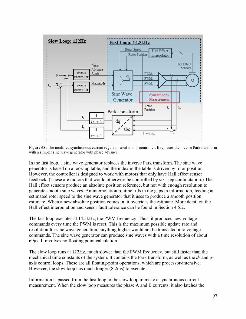
97

Figure 68: The modified synchronous current regulator used in this controller. It replaces the inverse Park transform with a simpler sine wave generator with phase advance.

In the fast loop, a sine wave generator replaces the inverse Park transform. The sine wave generator is based on a look-up table, and the index in the table is driven by rotor position. However, the controller is designed to work with motors that only have Hall effect sensor feedback. (These are motors that would otherwise be controlled by six-step commutation.) The Hall effect sensors produce an absolute position reference, but not with enough resolution to generate smooth sine waves. An interpolation routine fills in the gaps in information, feeding an estimated rotor speed to the sine wave generator that it uses to produce a smooth position estimate. When a new absolute position comes in, it overrides the estimate. More detail on the Hall effect interpolation and sensor fault tolerance can be found in Section 4.5.2.

The fast loop executes at 14.5kHz, the PWM frequency. Thus, it produces new voltage commands every time the PWM is reset. This is the maximum possible update rate and resolution for sine wave generation; anything higher would not be translated into voltage commands. The sine wave generator can produce sine waves with a time resolution of about 69μs. It involves no floating point calculation.

The slow loop runs at 122Hz, much slower than the PWM frequency, but still faster than the mechanical time constants of the system. It contains the Park transform, as well as the d- and q-axis control loops. These are all floating-point operations, which are processor-intensive. However, the slow loop has much longer (8.2ms) to execute.

Information is passed from the fast loop to the slow loop to make a synchronous current measurement. When the slow loop measures the phase A and B currents, it also latches the

98

instantaneous rotor position estimate and uses this value for the Park transformation. Even if the Park transformation takes many cycles to complete and the rotor moves during the processing, it is using the latched value of rotor position. This ensures that the current measurement is truly synchronous.

The inputs to the modified synchronous current regulator are unchanged: d-axis reference current is always zero and q-axis reference current is the torque command. Similarly, the two axes have their own independent control blocks. However, the output of these control blocks differs from those of the standard synchronous current regulator. In the standard method, a d-axis and q-axis command were established. Here, the outputs are a magnitude and phase angle for the sine wave generator. The magnitude is a simple scaling operation applied equally to all three PWM outputs. The phase is just a shift in the look-up table. These are processor-friendly operations that replace the inverse Park transformation in the standard synchronous current regulator.

It is important to note that this modification does actually change the fundamental control dynamics of the synchronous current regulator. Now, torque control is executed solely by adjusting the magnitude of the sine waves while phase control is handled independently. Assuming the loops are stable, the steady-state operating point is the same, being entirely driven by the references. What will be different is the transient response and command tracking.

Control loop stability may be affected, especially at high angles. This was a concern at first, since the modified controller seemingly couples the d- and q-axis control. Interestingly, though, two were already coupled by the motor inductance, since in either case the reference is current but the controller output is voltage.

Consider the affect of a step in the Iq reference with the standard synchronous current regulator. The q-axis controller will output an increased Vq. This will, due to motor inductance, show up as both Iq and Id. The d-axis controller will then modify Vd to correct for the extra d-axis current. These are both occurring “simultaneously,” with at most one control loop delay between a step on Iq and a correction on Vd. So it can still effectively drive Id to zero. But the two controllers are certainly coupled.

The modified synchronous current regulator, on the other hand, takes a step on Iq and outputs an increase in the magnitude of the total voltage vector. Since that vector may already have some phase advance angle from previous control actions, more of the current resulting from this step shows up on the q-axis. The d-axis controller separately modifies the phase advance angle to correct for any d-axis current. In some sense, this is actually less coupled than the standard synchronous current regulator, since it has built-in part of the expected current lag.

A more thorough stability analysis is beyond the scope of this report, but based on the above the modified controller is expected to be at least as stable as the standard synchronous current regulator under the same operating conditions. Testing with a high-RPM RC car motor, discussed in Section 4.7.2, has shown that the modified synchronous current regulator is still effective at high advance angles.

99

4.6 Data Acquisition and AnalysisOne of the most important features of a motor controller designed for motor or vehicle prototyping is integrated data acquisition. This is also a feature that clearly separates the controller developed for this study from commercially available options. Very few off-the-shelf controllers have capabilities for data acquisition, and those that do tend to be expensive. Another option is to add sensors and data acquisition capability to an existing motor controller, but in many cases this is redundant and also not cost affective. Consider the various parameters that a data acquisition system may target for evaluating a motor or controller:

System voltages. Most motor controllers already have some provisions for measuring battery voltage, even if they only use it as a low battery warning or cutoff. Additionally, the controller already “knows” the voltage being output to the various phases of a motor, since it is commanding the PWM signal.

System currents. Many (but not all) motor controllers have current measurement capability. Certainly, controllers that do current control have a current sensor built in. For BLDC control, one current sensor may suffice. To sense three-phase current for AC control, at least two sensors are required. (The third current must complete the zero sum.)

Motor speed. In the case of brushless motors, which are synchronous, the motor speed is also already “known” by the controller. It must be the electrical frequency divided by the number of pole pairs. An additional encoder or tachometer should not be necessary in most cases.

These measurements, which most controllers are already doing anyway, form the basis of the power analysis that can be used to evaluate the performance of a prototype motor. Allowing the controller to store this data is a simple step that does not require any additional hardware. This section discusses the integration of data acquisition into the case-study controller.

4.6.1 Integrated Wireless Data AcquisitionThe case study controller features integrated wireless data acquisition. Thought at first it may seem more difficult because of the wireless data transfer requirement, this method can actually be significantly less cumbersome than integrating on-board data storage. The controller uses a single digital 2.4GHz transceiver, picture in Figure 69, to transmit data. This transceiver (from the Digi XBee series) comes in two power options in nearly the same form factor. The higher-power transmitter uses slightly less than 700mW when transmitting and has an indoor range of 300ft (outdoor/line-of-site: 1 mile).

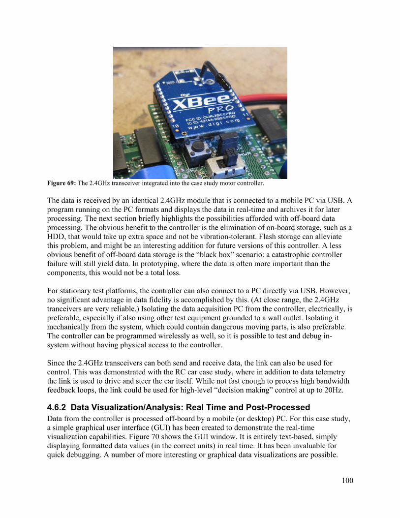
100

Figure 69: The 2.4GHz transceiver integrated into the case study motor controller.

The data is received by an identical 2.4GHz module that is connected to a mobile PC via USB. A program running on the PC formats and displays the data in real-time and archives it for later processing. The next section briefly highlights the possibilities afforded with off-board data processing. The obvious benefit to the controller is the elimination of on-board storage, such as a HDD, that would take up extra space and not be vibration-tolerant. Flash storage can alleviate this problem, and might be an interesting addition for future versions of this controller. A less obvious benefit of off-board data storage is the “black box” scenario: a catastrophic controller failure will still yield data. In prototyping, where the data is often more important than the components, this would not be a total loss.

For stationary test platforms, the controller can also connect to a PC directly via USB. However, no significant advantage in data fidelity is accomplished by this. (At close range, the 2.4GHz tranceivers are very reliable.) Isolating the data acquisition PC from the controller, electrically, is preferable, especially if also using other test equipment grounded to a wall outlet. Isolating it mechanically from the system, which could contain dangerous moving parts, is also preferable. The controller can be programmed wirelessly as well, so it is possible to test and debug in-system without having physical access to the controller.

Since the 2.4GHz transceivers can both send and receive data, the link can also be used for control. This was demonstrated with the RC car case study, where in addition to data telemetry the link is used to drive and steer the car itself. While not fast enough to process high bandwidth feedback loops, the link could be used for high-level “decision making” control at up to 20Hz.

4.6.2 Data Visualization/Analysis: Real Time and Post-ProcessedData from the controller is processed off-board by a mobile (or desktop) PC. For this case study, a simple graphical user interface (GUI) has been created to demonstrate the real-time visualization capabilities. Figure 70 shows the GUI window. It is entirely text-based, simply displaying formatted data values (in the correct units) in real time. It has been invaluable for quick debugging. A number of more interesting or graphical data visualizations are possible.

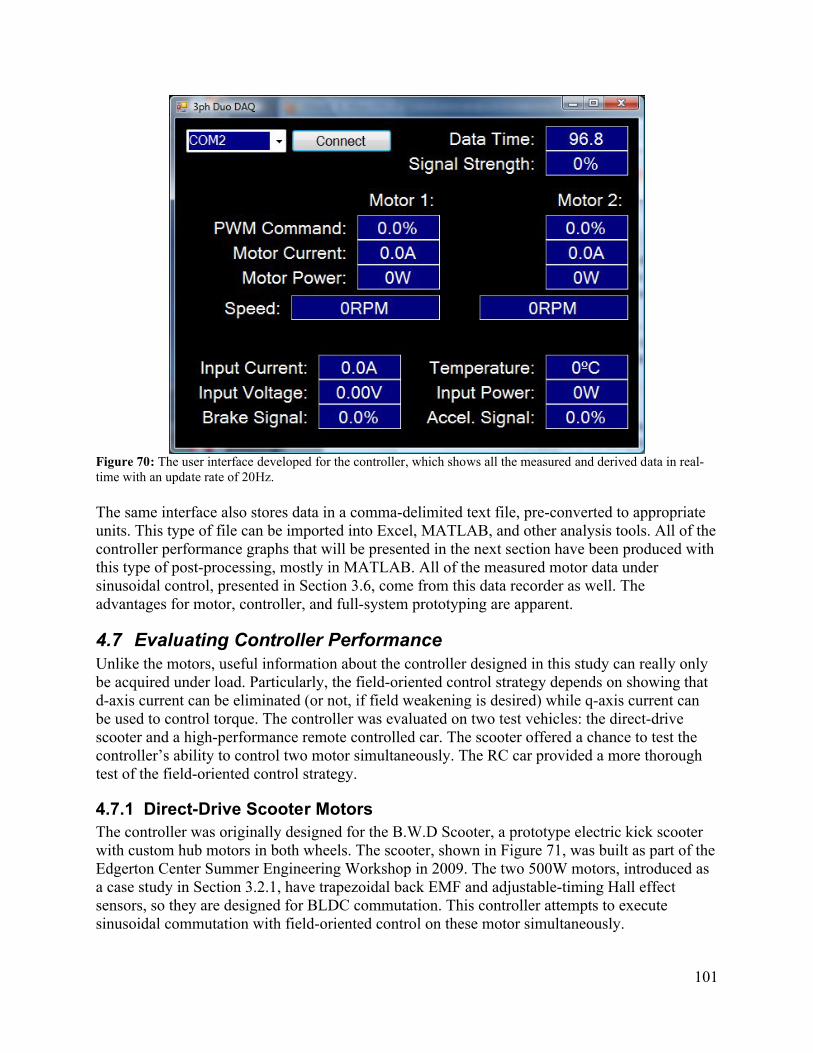
101

Figure 70: The user interface developed for the controller, which shows all the measured and derived data in real-time with an update rate of 20Hz.

The same interface also stores data in a comma-delimited text file, pre-converted to appropriate units. This type of file can be imported into Excel, MATLAB, and other analysis tools. All of the controller performance graphs that will be presented in the next section have been produced with this type of post-processing, mostly in MATLAB. All of the measured motor data under sinusoidal control, presented in Section 3.6, come from this data recorder as well. The advantages for motor, controller, and full-system prototyping are apparent.

4.7 Evaluating Controller PerformanceUnlike the motors, useful information about the controller designed in this study can really only be acquired under load. Particularly, the field-oriented control strategy depends on showing that d-axis current can be eliminated (or not, if field weakening is desired) while q-axis current can be used to control torque. The controller was evaluated on two test vehicles: the direct-drive scooter and a high-performance remote controlled car. The scooter offered a chance to test the controller’s ability to control two motor simultaneously. The RC car provided a more thorough test of the field-oriented control strategy.

4.7.1 Direct-Drive Scooter MotorsThe controller was originally designed for the B.W.D Scooter, a prototype electric kick scooter with custom hub motors in both wheels. The scooter, shown in Figure 71, was built as part of the Edgerton Center Summer Engineering Workshop in 2009. The two 500W motors, introduced as a case study in Section 3.2.1, have trapezoidal back EMF and adjustable-timing Hall effect sensors, so they are designed for BLDC commutation. This controller attempts to execute sinusoidal commutation with field-oriented control on these motor simultaneously.

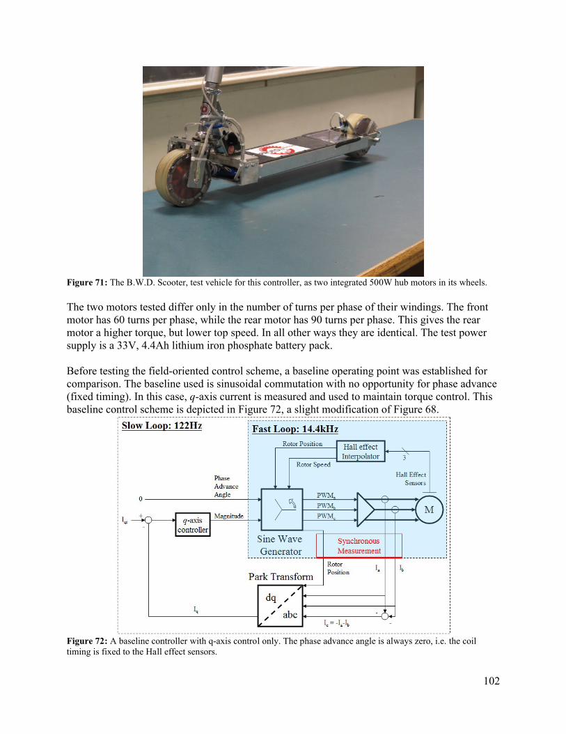
102

Figure 71: The B.W.D. Scooter, test vehicle for this controller, as two integrated 500W hub motors in its wheels.

The two motors tested differ only in the number of turns per phase of their windings. The front motor has 60 turns per phase, while the rear motor has 90 turns per phase. This gives the rear motor a higher torque, but lower top speed. In all other ways they are identical. The test power supply is a 33V, 4.4Ah lithium iron phosphate battery pack.

Before testing the field-oriented control scheme, a baseline operating point was established for comparison. The baseline used is sinusoidal commutation with no opportunity for phase advance (fixed timing). In this case, q-axis current is measured and used to maintain torque control. This baseline control scheme is depicted in Figure 72, a slight modification of Figure 68.

Figure 72: A baseline controller with q-axis control only. The phase advance angle is always zero, i.e. the coil timing is fixed to the Hall effect sensors.

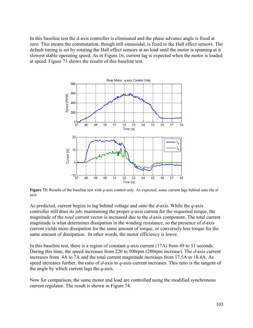
103

In this baseline test the d-axis controller is eliminated and the phase advance angle is fixed at zero. This means the commutation, though still sinusoidal, is fixed to the Hall effect sensors. The default timing is set by rotating the Hall effect sensors at no load until the motor is spinning at it slowest stable operating speed. As in Figure 16, current lag is expected when the motor is loaded at speed. Figure 73 shows the results of this baseline test.

Figure 73: Results of the baseline test with q-axis control only. As expected, some current lags behind onto the d-axis.

As predicted, current begins to lag behind voltage and onto the d-axis. While the q-axis controller still does its job, maintaining the proper q-axis current for the requested torque, the magnitude of the total current vector is increased due to the d-axis component. The total current magnitude is what determines dissipation in the winding resistance, so the presence of d-axis current yields more dissipation for the same amount of torque, or conversely less torque for the same amount of dissipation. In other words, the motor efficiency is lower.

In this baseline test, there is a region of constant q-axis current (17A) from 49 to 51 seconds. During this time, the speed increases from 220 to 500rpm (280rpm increase). The d-axis current increases from 4A to 7A and the total current magnitude increases from 17.5A to 18.4A. As speed increases further, the ratio of d-axis to q-axis current increases. This ratio is the tangent of the angle by which current lags the q-axis.

Now for comparison, the same motor and load are controlled using the modified synchronous current regulator. The result is shown in Figure 74.

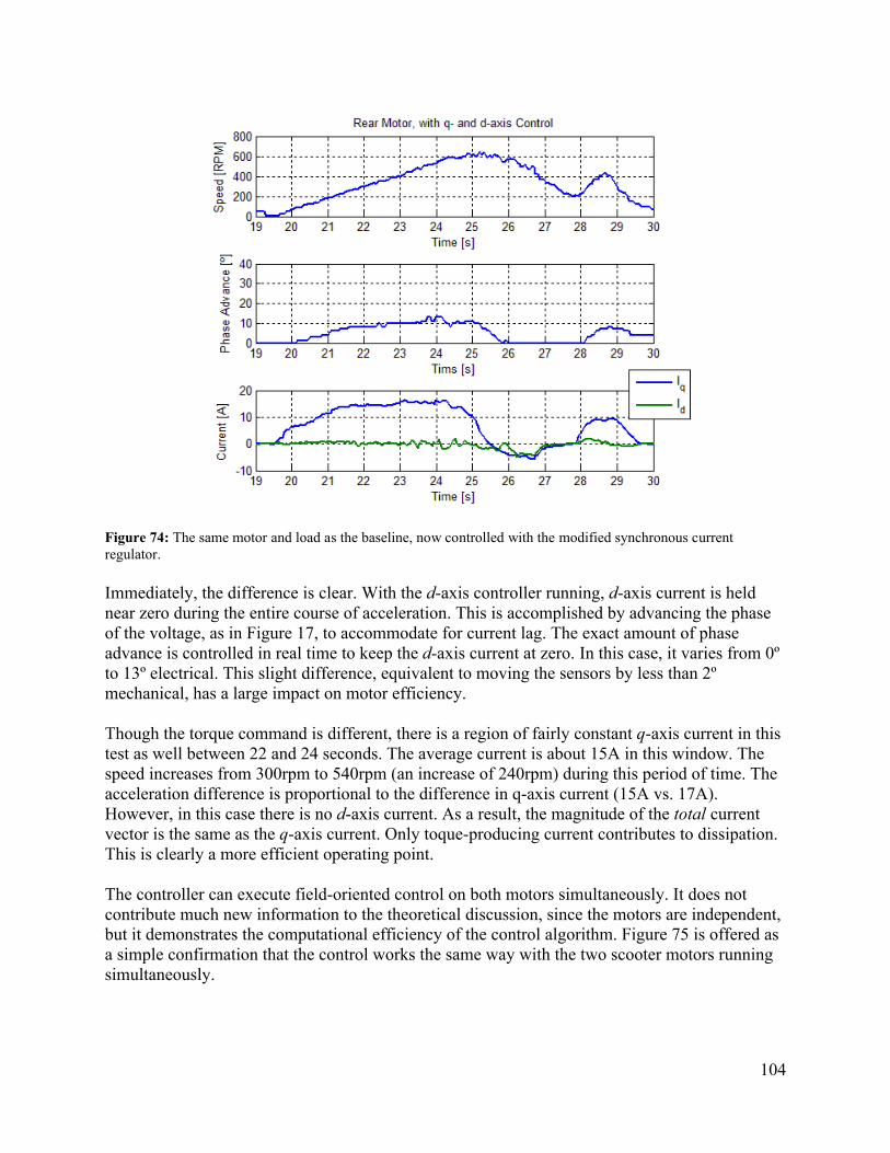
104

Figure 74: The same motor and load as the baseline, now controlled with the modified synchronous current regulator.

Immediately, the difference is clear. With the d-axis controller running, d-axis current is held near zero during the entire course of acceleration. This is accomplished by advancing the phase of the voltage, as in Figure 17, to accommodate for current lag. The exact amount of phase advance is controlled in real time to keep the d-axis current at zero. In this case, it varies from 0º to 13º electrical. This slight difference, equivalent to moving the sensors by less than 2º mechanical, has a large impact on motor efficiency.

Though the torque command is different, there is a region of fairly constant q-axis current in this test as well between 22 and 24 seconds. The average current is about 15A in this window. The speed increases from 300rpm to 540rpm (an increase of 240rpm) during this period of time. The acceleration difference is proportional to the difference in q-axis current (15A vs. 17A). However, in this case there is no d-axis current. As a result, the magnitude of the total current vector is the same as the q-axis current. Only toque-producing current contributes to dissipation. This is clearly a more efficient operating point.

The controller can execute field-oriented control on both motors simultaneously. It does not contribute much new information to the theoretical discussion, since the motors are independent, but it demonstrates the computational efficiency of the control algorithm. Figure 75 is offered as a simple confirmation that the control works the same way with the two scooter motors running simultaneously.

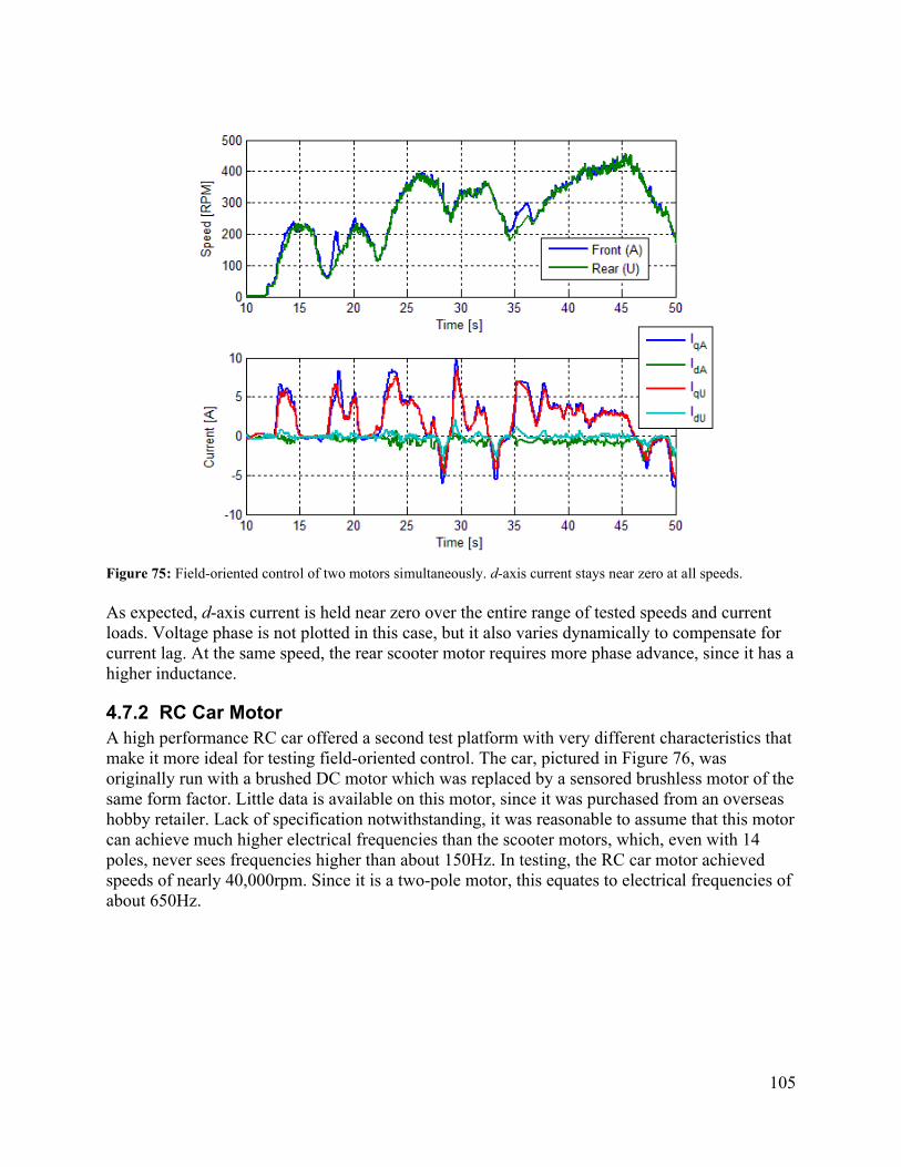
105

Figure 75: Field-oriented control of two motors simultaneously. d-axis current stays near zero at all speeds.

As expected, d-axis current is held near zero over the entire range of tested speeds and current loads. Voltage phase is not plotted in this case, but it also varies dynamically to compensate for current lag. At the same speed, the rear scooter motor requires more phase advance, since it has a higher inductance.

4.7.2 RC Car MotorA high performance RC car offered a second test platform with very different characteristics that make it more ideal for testing field-oriented control. The car, pictured in Figure 76, was originally run with a brushed DC motor which was replaced by a sensored brushless motor of the same form factor. Little data is available on this motor, since it was purchased from an overseas hobby retailer. Lack of specification notwithstanding, it was reasonable to assume that this motor can achieve much higher electrical frequencies than the scooter motors, which, even with 14 poles, never sees frequencies higher than about 150Hz. In testing, the RC car motor achieved speeds of nearly 40,000rpm. Since it is a two-pole motor, this equates to electrical frequencies of about 650Hz.

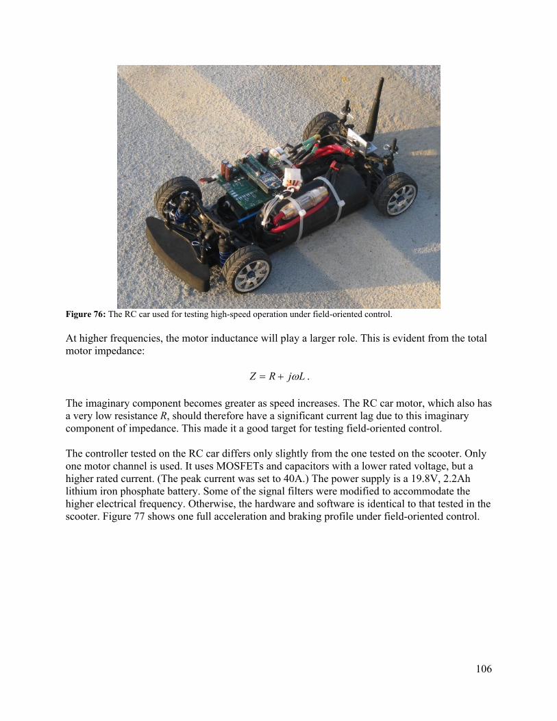
106

Figure 76: The RC car used for testing high-speed operation under field-oriented control.

At higher frequencies, the motor inductance will play a larger role. This is evident from the total motor impedance:

LjRZ .

The imaginary component becomes greater as speed increases. The RC car motor, which also has a very low resistance R, should therefore have a significant current lag due to this imaginary component of impedance. This made it a good target for testing field-oriented control.

The controller tested on the RC car differs only slightly from the one tested on the scooter. Only one motor channel is used. It uses MOSFETs and capacitors with a lower rated voltage, but a higher rated current. (The peak current was set to 40A.) The power supply is a 19.8V, 2.2Ah lithium iron phosphate battery. Some of the signal filters were modified to accommodate the higher electrical frequency. Otherwise, the hardware and software is identical to that tested in the scooter. Figure 77 shows one full acceleration and braking profile under field-oriented control.

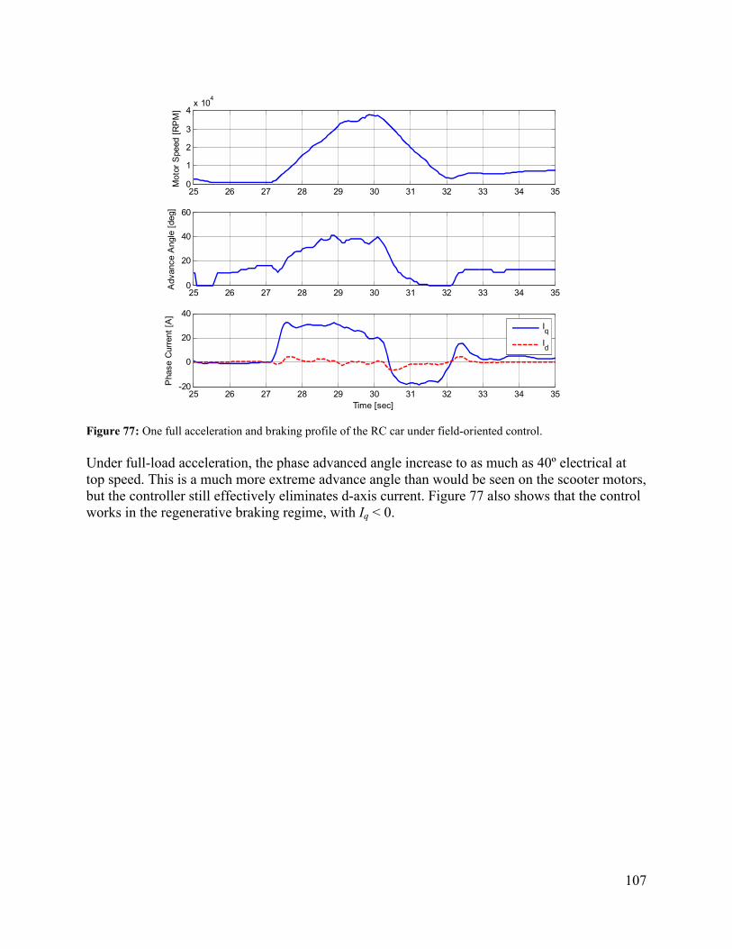
107

25 26 27 28 29 30 31 32 33 34 350

1

2

3

4x 10

4

Mot

or S

peed

[R

PM

]

25 26 27 28 29 30 31 32 33 34 350

20

40

60

Adv

ance

Ang

le [

deg]

25 26 27 28 29 30 31 32 33 34 35-20

0

20

40

Time [sec]

Pha

se C

urre

nt [

A]

Iq

Id

Figure 77: One full acceleration and braking profile of the RC car under field-oriented control.

Under full-load acceleration, the phase advanced angle increase to as much as 40º electrical at top speed. This is a much more extreme advance angle than would be seen on the scooter motors, but the controller still effectively eliminates d-axis current. Figure 77 also shows that the control works in the regenerative braking regime, with Iq < 0.

108

5 ConclusionsThis report has demonstrated an approach to brushless motor and motor control design and prototyping that, the author hopes, will be useful to others with similar interests. The methods are not meant to be an exhaustive treatment of electric machine theory, but rather a set of tools that are particularly handy for designing custom motors and controllers in-house, for low coast, and on a short design cycle. In other words, these are tools that enable individuals and labs for which motor design is not the primary focus to design motors and controllers.

In Section 2, some of the guiding physical principles behind electric motors and motor controllers were established and may serve as a good theoretical reference. However, a more complete treatment of electric machine theory can be found in [4] and [5]. A thorough understanding of the motor model is important for design as it is necessary to fit this model into the system optimization. This is true whether designing a motor from scratch or buying one from a catalog. Due to their simplicity, brushless motors are well-modeled in the electrical and mechanical domain. Their performance can be estimated with good accuracy from this model.

Two case studies were carried out that demonstrate the power of this motor model for designing custom brushless permanent magnet synchronous motors. In Section 3, the design process used for these motors was discussed in detail, showing various ways to predict the motor constant, resistance, and power rating. Rapid prototyping methods that enable in-house motor prototype fabrication allow for real-life evaluation of motor performance. In all cases, the motor constant of the case study motors was well-predicted by the motor model. In the case of the axial flux motor, a particular loss mechanism (eddy currents in flat wire) which was originally unaccounted-for made a large difference in the final performance of the motor. However, understanding the motor model helped troubleshoot this loss mechanism and will guide later iterations of this design.

In prototyping a motor controller, both mechanical and electrical constraints simultaneously guide the design. The design for a two channel brushless motor controller was developed in Section 4. This controller implements advanced control techniques on low-cost hardware. It allows motors with Hall effect sensors, originally designed to be operated with BLDC control, to instead use full sinusoidal field-oriented control. This has demonstrated advantages in performance, noise reduction, and efficiency. The controller uses a modified synchronous current regulator that has been optimized to run on fixed-point embedded processors. It has been successfully tested under load on both the scooter motors and a high-RPM remote control car motor.

This project has been an extremely rewarding pursuit for the author and no written report can fully capture the nature of the learning experience afforded by pursuing a hands-on motor and controller build. If there is an overall conclusion, it is that designing and fabricating a custom motor or controller solution, though not always called for by the application, is feasible and can reveal a much deeper understanding of electric motors, a key mechanical design component. For this reason, it is the author’s hope that others will find parts of this report useful for their own motor and motor control projects.

109

6 References[1] Finite Element Method Magnetics. http://www.femm.info/wiki/HomePage.

[2] The Edgerton Center. http://web.mit.edu/edgerton/main.html.

[3] Some of the Summer Engineering Workshop’s projects:A do-it-yourself self-balancing scooter: http://web.mit.edu/first/segway/.An electric go-kart with capacitive boost/brake: http://web.mit.edu/first/kart/.A direct-drive electric scooter with two hub motors: http://web.mit.edu/first/scooter/.

[4] Kirtley, James L. Lecture Notes for 6.685: Electric Machines. MIT OpenCourseWare.http://ocw.mit.edu/OcwWeb/Electrical-Engineering-and-Computer-Science/6-685Fall-2005/LectureNotes/index.htm.

[5] Mevey, James Robert. Sensorless Field Oriented Control of Brushless Permanent Magnet Synchronous Motors. S.M. Thesis, Kansas State University. 2009.

[6] For a good summary of possible slot/pole combinations, see the table at:http://fast-results.com/lnl/nutpol_e.htm.

[7] Guan, Charles Z. Project RazEr. http://www.etotheipiplusone.net/?cat=28.

[8] Lovatt, H.C., Ramsden, V.S, Mecrow, B.C. Desing of an In-Wheel Motor for a Solar Electric Vehicle.

[9] Woolmer, T.J., McCulloch, M.D. Analysis of the Yokeless and Segmented ArmatureMachine. Oxford University.

[10] Oxford Yasa Motors. http://www.oxfordyasamotors.com/.

[11] Proto Laminations, Inc. http://www.protolam.com/.

[12] Big Blue Saw. http://www.bigbluesaw.com/.

[13] IRFB3077PbF Datasheet. International Rectifier. http://www.irf.com/productinfo/datasheets/data/irfb3077pbf.pdf.

[14] GWM100-01X1 Datasheet. IXYS.http://download.siliconexpert.com/pdfs/2010/1/10/12/31/13/325/ixy_/manual/gwm100-01x1.pdf.

[15] 4QD-TEC: PWM speed control. 4QD. http://www.4qdtec.com/pwm-01.html#cap.

[16] Application Guide, Aluminum Electrolytic Capacitors. Cornell Dubilier.http://yces.case.edu/encycl/misc/c04-appguide.pdf.

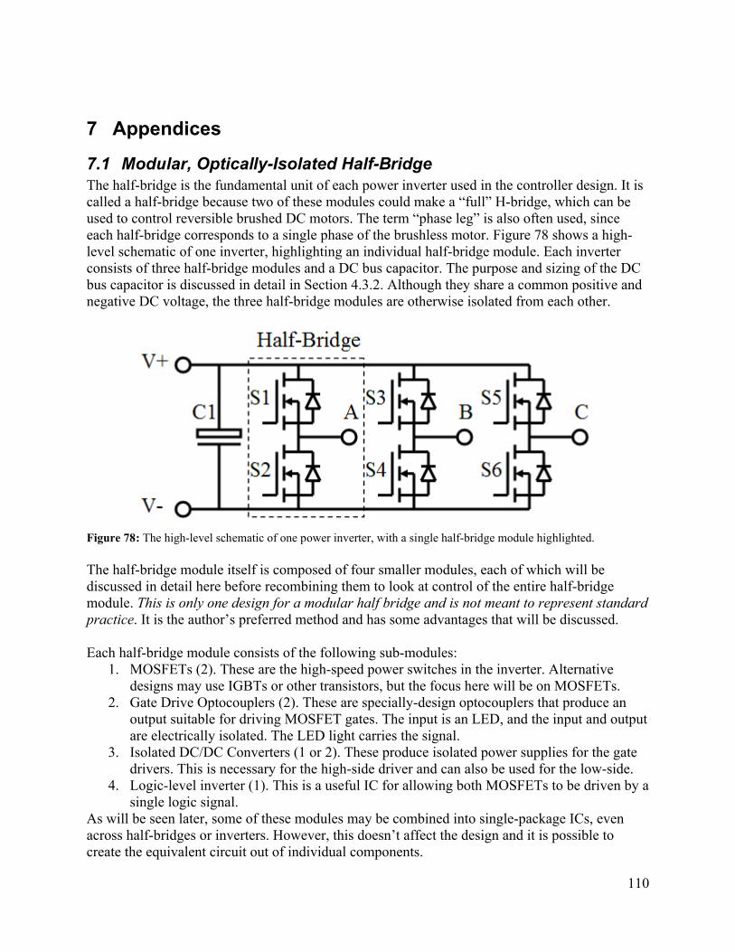
110

7 Appendices

7.1 Modular, Optically-Isolated Half-BridgeThe half-bridge is the fundamental unit of each power inverter used in the controller design. It is called a half-bridge because two of these modules could make a “full” H-bridge, which can be used to control reversible brushed DC motors. The term “phase leg” is also often used, since each half-bridge corresponds to a single phase of the brushless motor. Figure 78 shows a high-level schematic of one inverter, highlighting an individual half-bridge module. Each inverter consists of three half-bridge modules and a DC bus capacitor. The purpose and sizing of the DC bus capacitor is discussed in detail in Section 4.3.2. Although they share a common positive and negative DC voltage, the three half-bridge modules are otherwise isolated from each other.

Figure 78: The high-level schematic of one power inverter, with a single half-bridge module highlighted.

The half-bridge module itself is composed of four smaller modules, each of which will be discussed in detail here before recombining them to look at control of the entire half-bridge module. This is only one design for a modular half bridge and is not meant to represent standard practice. It is the author’s preferred method and has some advantages that will be discussed.

Each half-bridge module consists of the following sub-modules:1. MOSFETs (2). These are the high-speed power switches in the inverter. Alternative

designs may use IGBTs or other transistors, but the focus here will be on MOSFETs.2. Gate Drive Optocouplers (2). These are specially-design optocouplers that produce an

output suitable for driving MOSFET gates. The input is an LED, and the input and output are electrically isolated. The LED light carries the signal.

3. Isolated DC/DC Converters (1 or 2). These produce isolated power supplies for the gate drivers. This is necessary for the high-side driver and can also be used for the low-side.

4. Logic-level inverter (1). This is a useful IC for allowing both MOSFETs to be driven by a single logic signal.

As will be seen later, some of these modules may be combined into single-package ICs, even across half-bridges or inverters. However, this doesn’t affect the design and it is possible to create the equivalent circuit out of individual components.

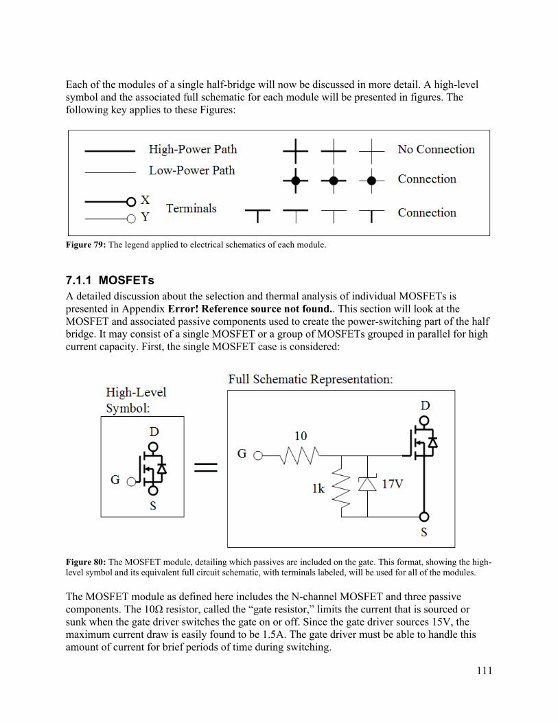
111

Each of the modules of a single half-bridge will now be discussed in more detail. A high-level symbol and the associated full schematic for each module will be presented in figures. The following key applies to these Figures:

Figure 79: The legend applied to electrical schematics of each module.

7.1.1 MOSFETsA detailed discussion about the selection and thermal analysis of individual MOSFETs is presented in Appendix Error! Reference source not found.. This section will look at the MOSFET and associated passive components used to create the power-switching part of the half bridge. It may consist of a single MOSFET or a group of MOSFETs grouped in parallel for high current capacity. First, the single MOSFET case is considered:

Figure 80: The MOSFET module, detailing which passives are included on the gate. This format, showing the high-level symbol and its equivalent full circuit schematic, with terminals labeled, will be used for all of the modules.

The MOSFET module as defined here includes the N-channel MOSFET and three passive components. The 10Ω resistor, called the “gate resistor,” limits the current that is sourced or sunk when the gate driver switches the gate on or off. Since the gate driver sources 15V, the maximum current draw is easily found to be 1.5A. The gate driver must be able to handle this amount of current for brief periods of time during switching.

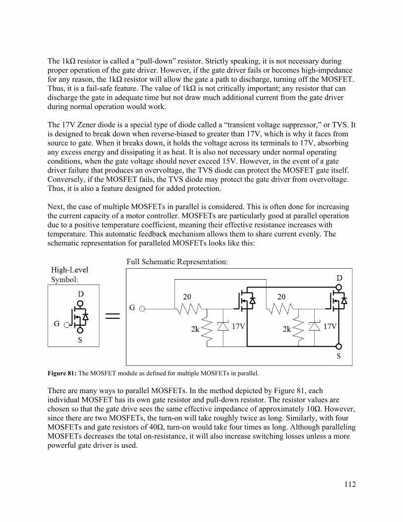
112

The 1kΩ resistor is called a “pull-down” resistor. Strictly speaking, it is not necessary during proper operation of the gate driver. However, if the gate driver fails or becomes high-impedance for any reason, the 1kΩ resistor will allow the gate a path to discharge, turning off the MOSFET. Thus, it is a fail-safe feature. The value of 1kΩ is not critically important; any resistor that can discharge the gate in adequate time but not draw much additional current from the gate driver during normal operation would work.

The 17V Zener diode is a special type of diode called a “transient voltage suppressor,” or TVS. It is designed to break down when reverse-biased to greater than 17V, which is why it faces from source to gate. When it breaks down, it holds the voltage across its terminals to 17V, absorbing any excess energy and dissipating it as heat. It is also not necessary under normal operating conditions, when the gate voltage should never exceed 15V. However, in the event of a gate driver failure that produces an overvoltage, the TVS diode can protect the MOSFET gate itself. Conversely, if the MOSFET fails, the TVS diode may protect the gate driver from overvoltage. Thus, it is also a feature designed for added protection.

Next, the case of multiple MOSFETs in parallel is considered. This is often done for increasing the current capacity of a motor controller. MOSFETs are particularly good at parallel operation due to a positive temperature coefficient, meaning their effective resistance increases with temperature. This automatic feedback mechanism allows them to share current evenly. The schematic representation for paralleled MOSFETs looks like this:

Figure 81: The MOSFET module as defined for multiple MOSFETs in parallel.

There are many ways to parallel MOSFETs. In the method depicted by Figure 81, each individual MOSFET has its own gate resistor and pull-down resistor. The resistor values are chosen so that the gate drive sees the same effective impedance of approximately 10Ω. However, since there are two MOSFETs, the turn-on will take roughly twice as long. Similarly, with four MOSFETs and gate resistors of 40Ω, turn-on would take four times as long. Although paralleling MOSFETs decreases the total on-resistance, it will also increase switching losses unless a more powerful gate driver is used.

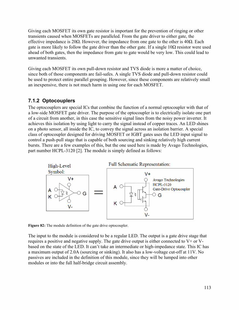
113

Giving each MOSFET its own gate resistor is important for the prevention of ringing or other transients caused when MOSFETs are paralleled. From the gate driver to either gate, the effective impedance is 20Ω. However, the impedance from one gate to the other is 40Ω. Each gate is more likely to follow the gate driver than the other gate. If a single 10Ω resistor were used ahead of both gates, then the impedance from gate to gate would be very low. This could lead to unwanted transients.

Giving each MOSFET its own pull-down resistor and TVS diode is more a matter of choice, since both of those components are fail-safes. A single TVS diode and pull-down resistor could be used to protect entire parallel grouping. However, since these components are relatively small an inexpensive, there is not much harm in using one for each MOSFET.

7.1.2 OptocouplersThe optocouplers are special ICs that combine the function of a normal optocoupler with that of a low-side MOSFET gate driver. The purpose of the optocoupler is to electrically isolate one part of a circuit from another, in this case the sensitive signal lines from the noisy power inverter. It achieves this isolation by using light to carry the signal instead of copper traces. An LED shines on a photo sensor, all inside the IC, to convey the signal across an isolation barrier. A special class of optocoupler designed for driving MOSFET or IGBT gates uses the LED input signal to control a push-pull stage that is capable of both sourcing and sinking relatively high current bursts. There are a few examples of this, but the one used here is made by Avago Technologies, part number HCPL-3120 [2]. The module is simply defined as follows:

Figure 82: The module definition of the gate drive optocoupler.

The input to the module is considered to be a regular LED. The output is a gate drive stage that requires a positive and negative supply. The gate drive output is either connected to V+ or V-based on the state of the LED. It can’t take an intermediate or high-impedance state. This IC has a maximum output of 2.0A (sourcing or sinking). It also has a low-voltage cut-off at 11V. No passives are included in the definition of this module, since they will be lumped into other modules or into the full half-bridge circuit assembly.

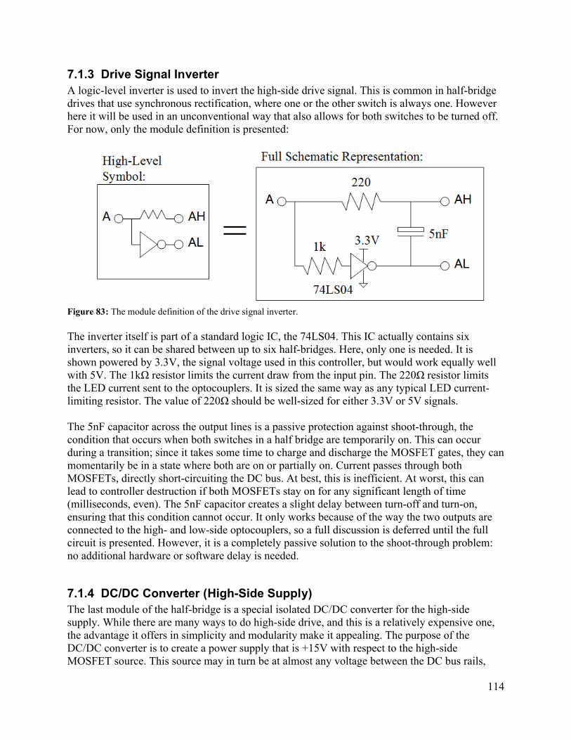
114

7.1.3 Drive Signal InverterA logic-level inverter is used to invert the high-side drive signal. This is common in half-bridge drives that use synchronous rectification, where one or the other switch is always one. However here it will be used in an unconventional way that also allows for both switches to be turned off. For now, only the module definition is presented:

Figure 83: The module definition of the drive signal inverter.

The inverter itself is part of a standard logic IC, the 74LS04. This IC actually contains six inverters, so it can be shared between up to six half-bridges. Here, only one is needed. It is shown powered by 3.3V, the signal voltage used in this controller, but would work equally well with 5V. The 1kΩ resistor limits the current draw from the input pin. The 220Ω resistor limits the LED current sent to the optocouplers. It is sized the same way as any typical LED current-limiting resistor. The value of 220Ω should be well-sized for either 3.3V or 5V signals.

The 5nF capacitor across the output lines is a passive protection against shoot-through, the condition that occurs when both switches in a half bridge are temporarily on. This can occur during a transition; since it takes some time to charge and discharge the MOSFET gates, they can momentarily be in a state where both are on or partially on. Current passes through both MOSFETs, directly short-circuiting the DC bus. At best, this is inefficient. At worst, this can lead to controller destruction if both MOSFETs stay on for any significant length of time (milliseconds, even). The 5nF capacitor creates a slight delay between turn-off and turn-on, ensuring that this condition cannot occur. It only works because of the way the two outputs are connected to the high- and low-side optocouplers, so a full discussion is deferred until the full circuit is presented. However, it is a completely passive solution to the shoot-through problem: no additional hardware or software delay is needed.

7.1.4 DC/DC Converter (High-Side Supply)The last module of the half-bridge is a special isolated DC/DC converter for the high-side supply. While there are many ways to do high-side drive, and this is a relatively expensive one, the advantage it offers in simplicity and modularity make it appealing. The purpose of the DC/DC converter is to create a power supply that is +15V with respect to the high-side MOSFET source. This source may in turn be at almost any voltage between the DC bus rails,

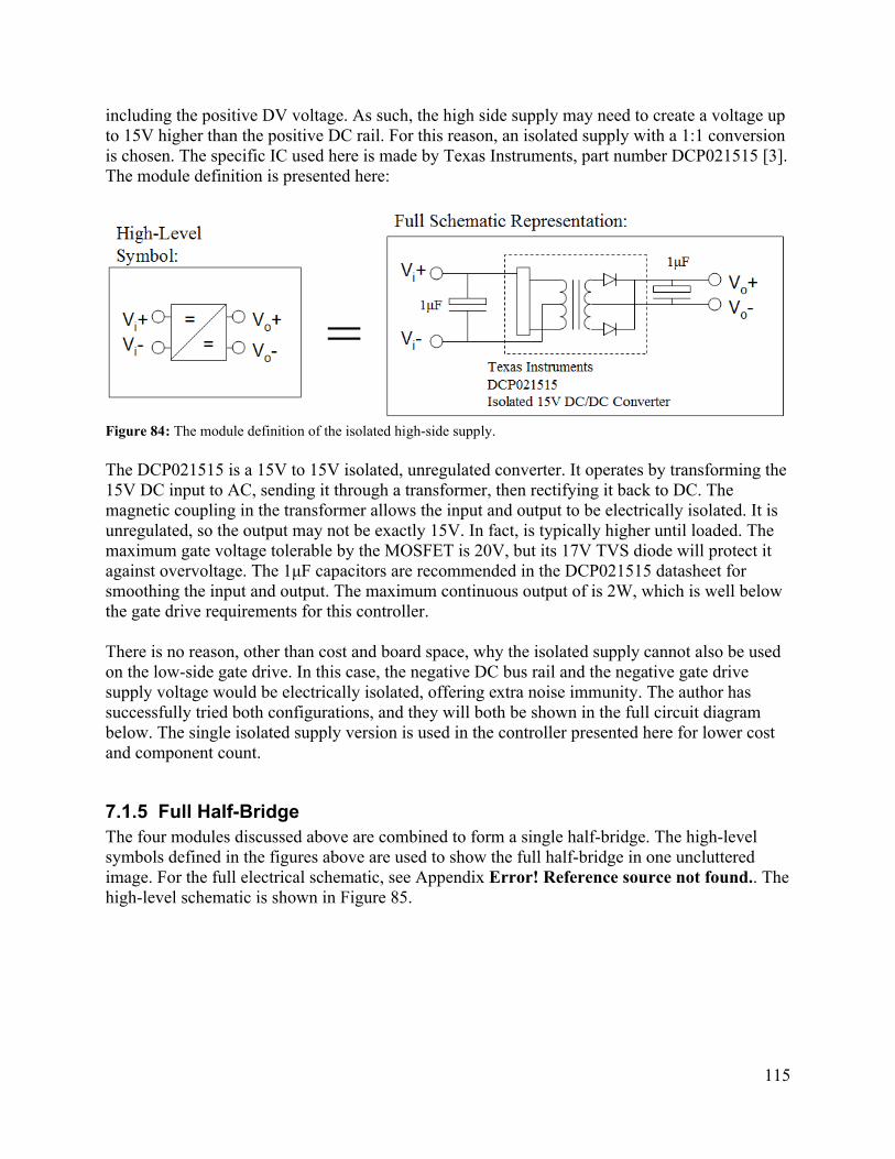
115

including the positive DV voltage. As such, the high side supply may need to create a voltage up to 15V higher than the positive DC rail. For this reason, an isolated supply with a 1:1 conversion is chosen. The specific IC used here is made by Texas Instruments, part number DCP021515 [3]. The module definition is presented here:

Figure 84: The module definition of the isolated high-side supply.

The DCP021515 is a 15V to 15V isolated, unregulated converter. It operates by transforming the 15V DC input to AC, sending it through a transformer, then rectifying it back to DC. The magnetic coupling in the transformer allows the input and output to be electrically isolated. It is unregulated, so the output may not be exactly 15V. In fact, is typically higher until loaded. The maximum gate voltage tolerable by the MOSFET is 20V, but its 17V TVS diode will protect it against overvoltage. The 1μF capacitors are recommended in the DCP021515 datasheet for smoothing the input and output. The maximum continuous output of is 2W, which is well below the gate drive requirements for this controller.

There is no reason, other than cost and board space, why the isolated supply cannot also be used on the low-side gate drive. In this case, the negative DC bus rail and the negative gate drive supply voltage would be electrically isolated, offering extra noise immunity. The author has successfully tried both configurations, and they will both be shown in the full circuit diagram below. The single isolated supply version is used in the controller presented here for lower cost and component count.

7.1.5 Full Half-BridgeThe four modules discussed above are combined to form a single half-bridge. The high-level symbols defined in the figures above are used to show the full half-bridge in one uncluttered image. For the full electrical schematic, see Appendix Error! Reference source not found.. The high-level schematic is shown in Figure 85.

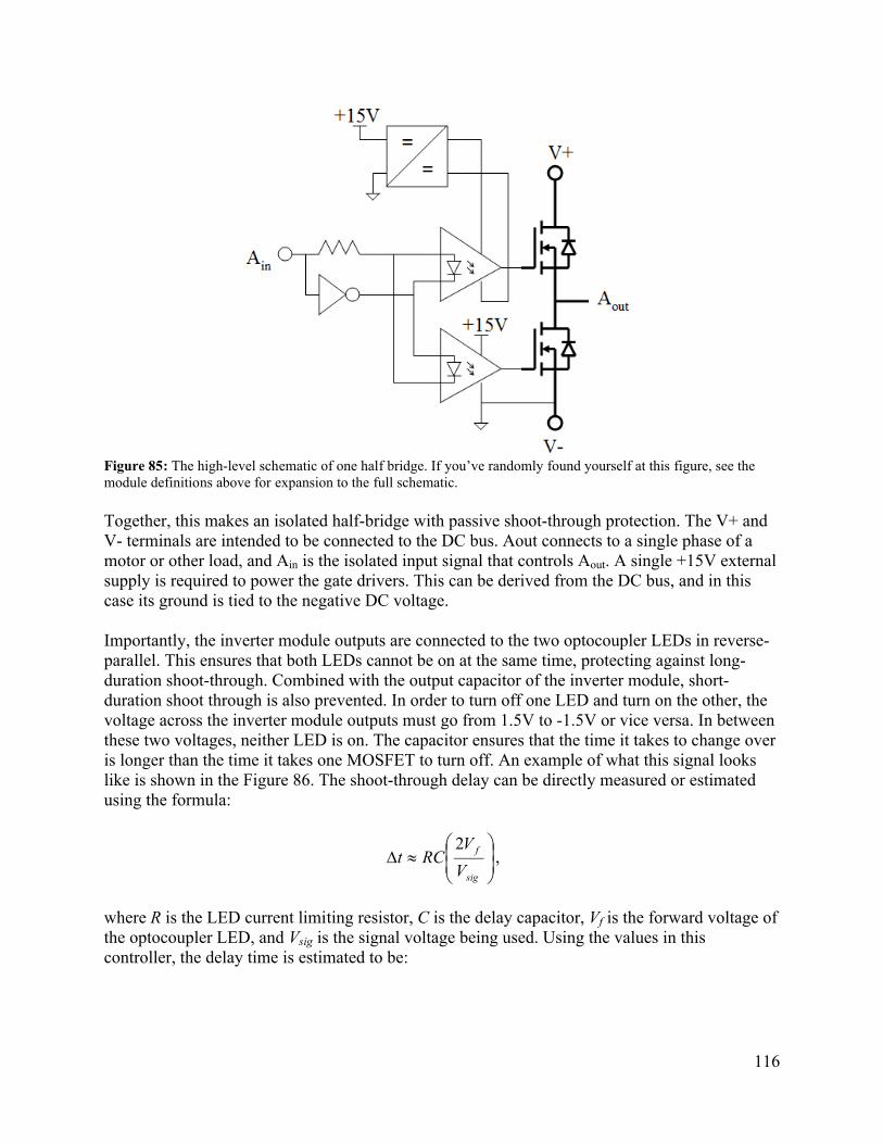
116

Figure 85: The high-level schematic of one half bridge. If you’ve randomly found yourself at this figure, see the module definitions above for expansion to the full schematic.

Together, this makes an isolated half-bridge with passive shoot-through protection. The V+ and V- terminals are intended to be connected to the DC bus. Aout connects to a single phase of a motor or other load, and Ain is the isolated input signal that controls Aout. A single +15V external supply is required to power the gate drivers. This can be derived from the DC bus, and in this case its ground is tied to the negative DC voltage.

Importantly, the inverter module outputs are connected to the two optocoupler LEDs in reverse-parallel. This ensures that both LEDs cannot be on at the same time, protecting against long-duration shoot-through. Combined with the output capacitor of the inverter module, short-duration shoot through is also prevented. In order to turn off one LED and turn on the other, the voltage across the inverter module outputs must go from 1.5V to -1.5V or vice versa. In between these two voltages, neither LED is on. The capacitor ensures that the time it takes to change over is longer than the time it takes one MOSFET to turn off. An example of what this signal looks like is shown in the Figure 86. The shoot-through delay can be directly measured or estimated using the formula:

sig

f

V

VRCt

2,

where R is the LED current limiting resistor, C is the delay capacitor, Vf is the forward voltage of the optocoupler LED, and Vsig is the signal voltage being used. Using the values in this controller, the delay time is estimated to be:

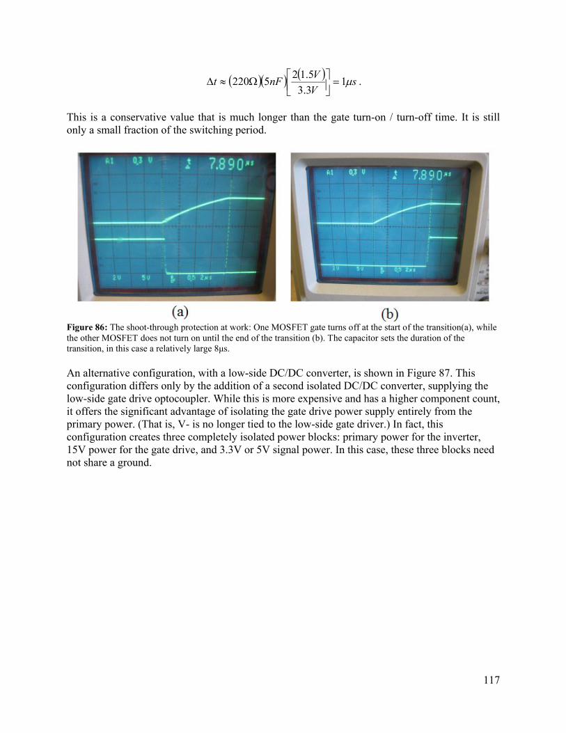
117

s

V

VnFt 1

3.3

5.125220

.

This is a conservative value that is much longer than the gate turn-on / turn-off time. It is still only a small fraction of the switching period.

Figure 86: The shoot-through protection at work: One MOSFET gate turns off at the start of the transition(a), while the other MOSFET does not turn on until the end of the transition (b). The capacitor sets the duration of the transition, in this case a relatively large 8μs.

An alternative configuration, with a low-side DC/DC converter, is shown in Figure 87. This configuration differs only by the addition of a second isolated DC/DC converter, supplying the low-side gate drive optocoupler. While this is more expensive and has a higher component count, it offers the significant advantage of isolating the gate drive power supply entirely from the primary power. (That is, V- is no longer tied to the low-side gate driver.) In fact, this configuration creates three completely isolated power blocks: primary power for the inverter, 15V power for the gate drive, and 3.3V or 5V signal power. In this case, these three blocks need not share a ground.

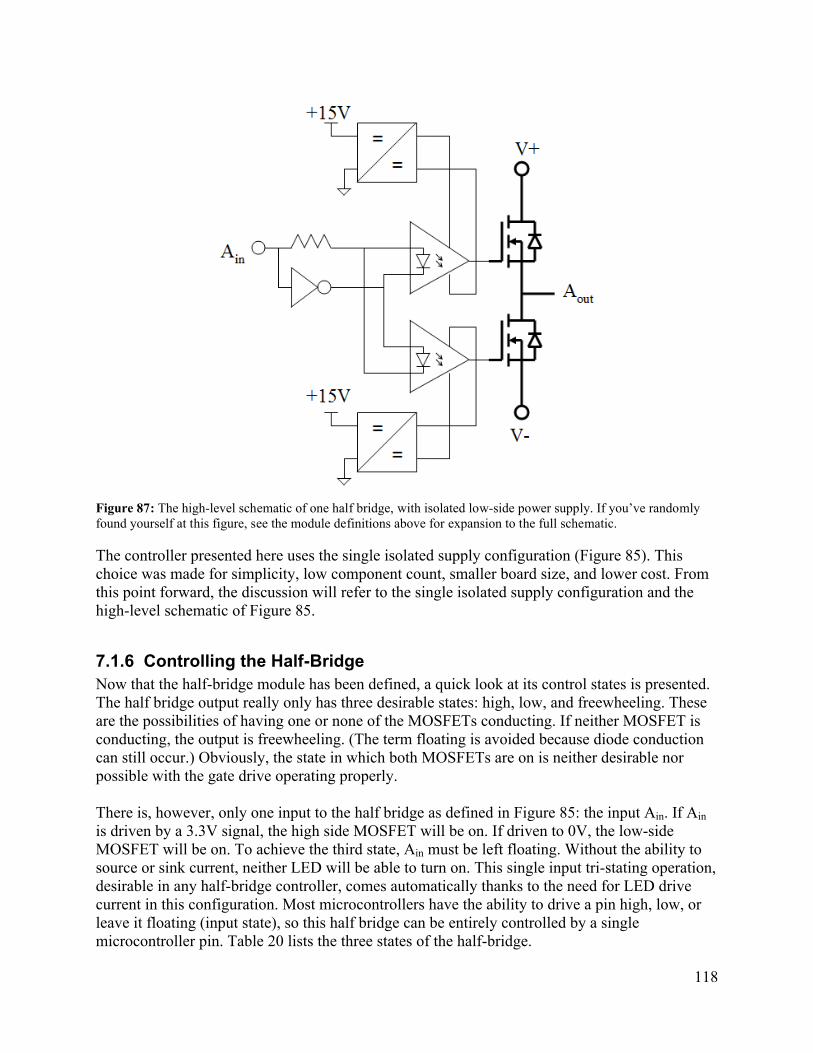
118

Figure 87: The high-level schematic of one half bridge, with isolated low-side power supply. If you’ve randomly found yourself at this figure, see the module definitions above for expansion to the full schematic.

The controller presented here uses the single isolated supply configuration (Figure 85). This choice was made for simplicity, low component count, smaller board size, and lower cost. From this point forward, the discussion will refer to the single isolated supply configuration and the high-level schematic of Figure 85.

7.1.6 Controlling the Half-BridgeNow that the half-bridge module has been defined, a quick look at its control states is presented. The half bridge output really only has three desirable states: high, low, and freewheeling. These are the possibilities of having one or none of the MOSFETs conducting. If neither MOSFET is conducting, the output is freewheeling. (The term floating is avoided because diode conduction can still occur.) Obviously, the state in which both MOSFETs are on is neither desirable nor possible with the gate drive operating properly.

There is, however, only one input to the half bridge as defined in Figure 85: the input Ain. If Ain

is driven by a 3.3V signal, the high side MOSFET will be on. If driven to 0V, the low-side MOSFET will be on. To achieve the third state, Ain must be left floating. Without the ability to source or sink current, neither LED will be able to turn on. This single input tri-stating operation, desirable in any half-bridge controller, comes automatically thanks to the need for LED drive current in this configuration. Most microcontrollers have the ability to drive a pin high, low, or leave it floating (input state), so this half bridge can be entirely controlled by a single microcontroller pin. Table 20 lists the three states of the half-bridge.

119

Table 20: The three half-bridge states.

Input Ain Output Aout Description3.3V V+ High-side MOSFET is on.

0V V- Low-side MOSFET is on.Float Freewheel Neither MOSFET is on. Output may voltage

undetermined. Diode conduction may still occur!

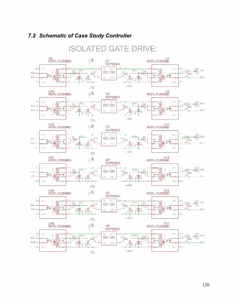
120

7.2 Schematic of Case Study Controller

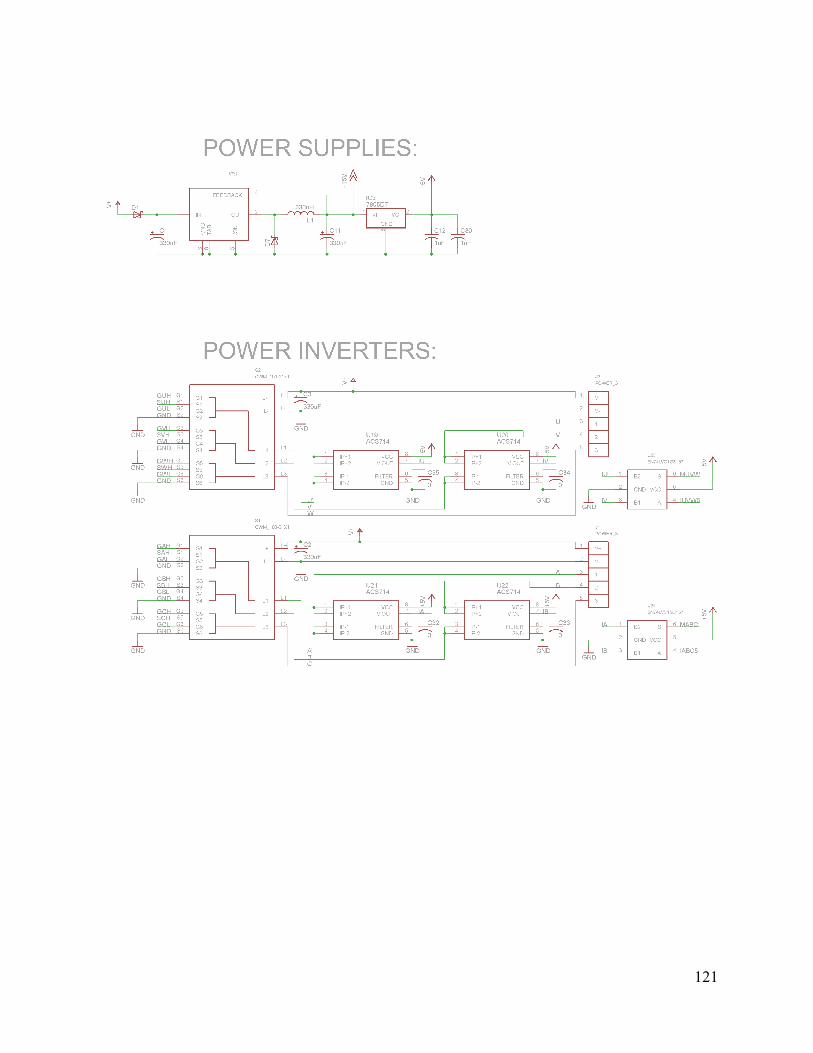
121

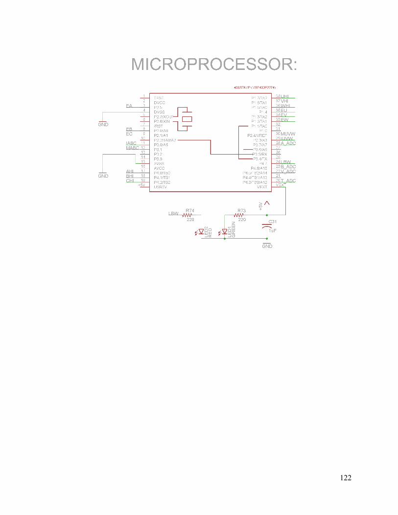
122

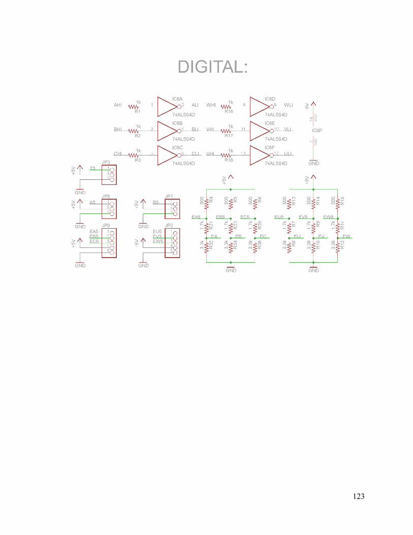
123

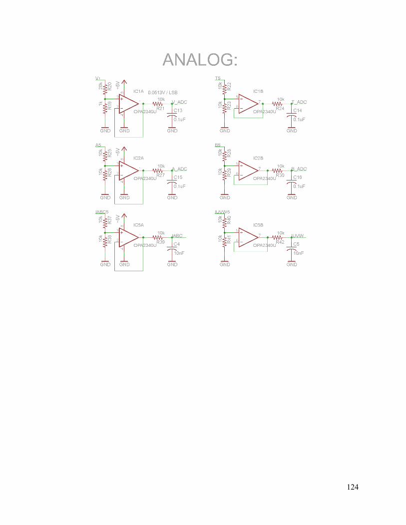
124

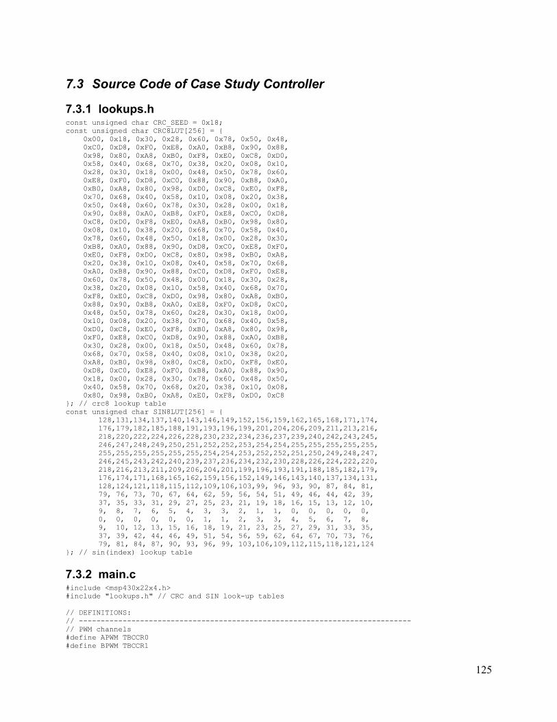
125

7.3 Source Code of Case Study Controller

7.3.1 lookups.hconst unsigned char CRC_SEED = 0x18;const unsigned char CRC8LUT[256] = { 0x00, 0x18, 0x30, 0x28, 0x60, 0x78, 0x50, 0x48, 0xC0, 0xD8, 0xF0, 0xE8, 0xA0, 0xB8, 0x90, 0x88, 0x98, 0x80, 0xA8, 0xB0, 0xF8, 0xE0, 0xC8, 0xD0, 0x58, 0x40, 0x68, 0x70, 0x38, 0x20, 0x08, 0x10, 0x28, 0x30, 0x18, 0x00, 0x48, 0x50, 0x78, 0x60, 0xE8, 0xF0, 0xD8, 0xC0, 0x88, 0x90, 0xB8, 0xA0, 0xB0, 0xA8, 0x80, 0x98, 0xD0, 0xC8, 0xE0, 0xF8, 0x70, 0x68, 0x40, 0x58, 0x10, 0x08, 0x20, 0x38, 0x50, 0x48, 0x60, 0x78, 0x30, 0x28, 0x00, 0x18, 0x90, 0x88, 0xA0, 0xB8, 0xF0, 0xE8, 0xC0, 0xD8, 0xC8, 0xD0, 0xF8, 0xE0, 0xA8, 0xB0, 0x98, 0x80, 0x08, 0x10, 0x38, 0x20, 0x68, 0x70, 0x58, 0x40, 0x78, 0x60, 0x48, 0x50, 0x18, 0x00, 0x28, 0x30, 0xB8, 0xA0, 0x88, 0x90, 0xD8, 0xC0, 0xE8, 0xF0, 0xE0, 0xF8, 0xD0, 0xC8, 0x80, 0x98, 0xB0, 0xA8, 0x20, 0x38, 0x10, 0x08, 0x40, 0x58, 0x70, 0x68, 0xA0, 0xB8, 0x90, 0x88, 0xC0, 0xD8, 0xF0, 0xE8, 0x60, 0x78, 0x50, 0x48, 0x00, 0x18, 0x30, 0x28, 0x38, 0x20, 0x08, 0x10, 0x58, 0x40, 0x68, 0x70, 0xF8, 0xE0, 0xC8, 0xD0, 0x98, 0x80, 0xA8, 0xB0, 0x88, 0x90, 0xB8, 0xA0, 0xE8, 0xF0, 0xD8, 0xC0, 0x48, 0x50, 0x78, 0x60, 0x28, 0x30, 0x18, 0x00, 0x10, 0x08, 0x20, 0x38, 0x70, 0x68, 0x40, 0x58, 0xD0, 0xC8, 0xE0, 0xF8, 0xB0, 0xA8, 0x80, 0x98, 0xF0, 0xE8, 0xC0, 0xD8, 0x90, 0x88, 0xA0, 0xB8, 0x30, 0x28, 0x00, 0x18, 0x50, 0x48, 0x60, 0x78, 0x68, 0x70, 0x58, 0x40, 0x08, 0x10, 0x38, 0x20, 0xA8, 0xB0, 0x98, 0x80, 0xC8, 0xD0, 0xF8, 0xE0, 0xD8, 0xC0, 0xE8, 0xF0, 0xB8, 0xA0, 0x88, 0x90, 0x18, 0x00, 0x28, 0x30, 0x78, 0x60, 0x48, 0x50, 0x40, 0x58, 0x70, 0x68, 0x20, 0x38, 0x10, 0x08, 0x80, 0x98, 0xB0, 0xA8, 0xE0, 0xF8, 0xD0, 0xC8}; // crc8 lookup tableconst unsigned char SIN8LUT[256] = {

128,131,134,137,140,143,146,149,152,156,159,162,165,168,171,174,176,179,182,185,188,191,193,196,199,201,204,206,209,211,213,216,218,220,222,224,226,228,230,232,234,236,237,239,240,242,243,245,246,247,248,249,250,251,252,252,253,254,254,255,255,255,255,255,255,255,255,255,255,255,254,254,253,252,252,251,250,249,248,247,246,245,243,242,240,239,237,236,234,232,230,228,226,224,222,220,218,216,213,211,209,206,204,201,199,196,193,191,188,185,182,179,176,174,171,168,165,162,159,156,152,149,146,143,140,137,134,131,128,124,121,118,115,112,109,106,103,99, 96, 93, 90, 87, 84, 81, 79, 76, 73, 70, 67, 64, 62, 59, 56, 54, 51, 49, 46, 44, 42, 39, 37, 35, 33, 31, 29, 27, 25, 23, 21, 19, 18, 16, 15, 13, 12, 10, 9, 8, 7, 6, 5, 4, 3, 3, 2, 1, 1, 0, 0, 0, 0, 0, 0, 0, 0, 0, 0, 0, 1, 1, 2, 3, 3, 4, 5, 6, 7, 8, 9, 10, 12, 13, 15, 16, 18, 19, 21, 23, 25, 27, 29, 31, 33, 35, 37, 39, 42, 44, 46, 49, 51, 54, 56, 59, 62, 64, 67, 70, 73, 76, 79, 81, 84, 87, 90, 93, 96, 99, 103,106,109,112,115,118,121,124

}; // sin(index) lookup table

7.3.2 main.c#include <msp430x22x4.h>#include "lookups.h" // CRC and SIN look-up tables

// DEFINITIONS:// ----------------------------------------------------------------------------// PWM channels#define APWM TBCCR0#define BPWM TBCCR1

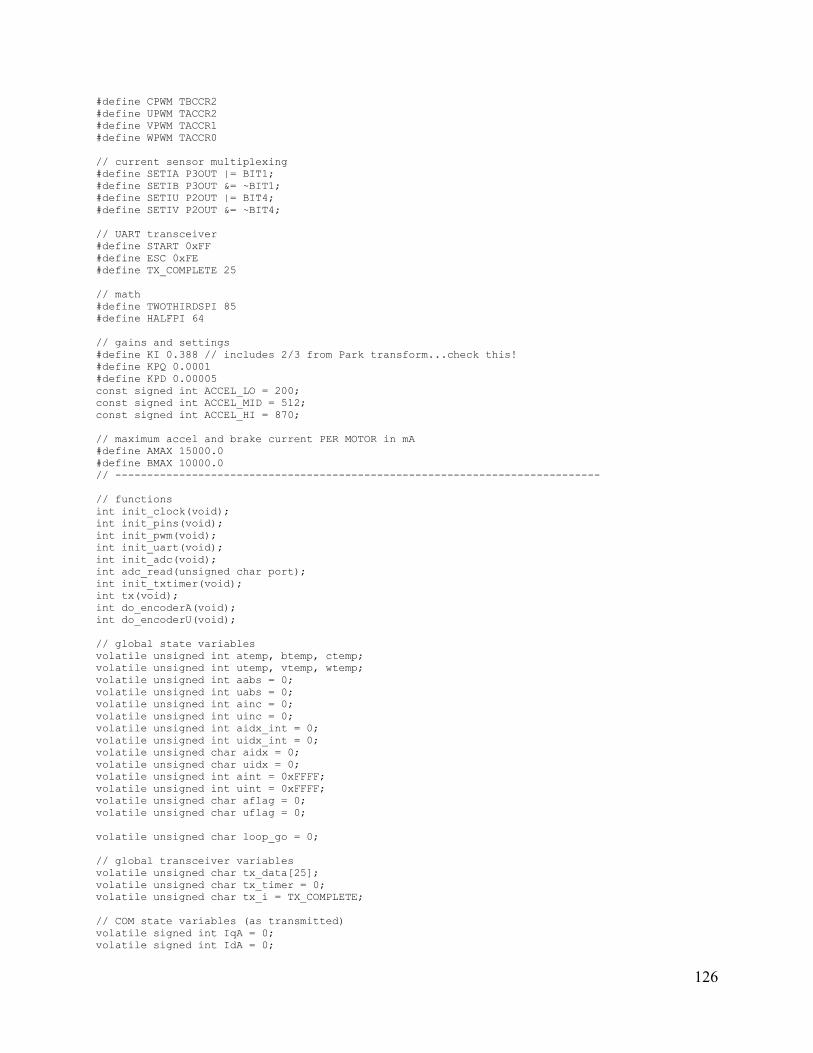
126

#define CPWM TBCCR2#define UPWM TACCR2#define VPWM TACCR1#define WPWM TACCR0

// current sensor multiplexing#define SETIA P3OUT |= BIT1;#define SETIB P3OUT &= ~BIT1;#define SETIU P2OUT |= BIT4;#define SETIV P2OUT &= ~BIT4;

// UART transceiver#define START 0xFF#define ESC 0xFE#define TX_COMPLETE 25

// math#define TWOTHIRDSPI 85#define HALFPI 64

// gains and settings#define KI 0.388 // includes 2/3 from Park transform...check this!#define KPQ 0.0001#define KPD 0.00005const signed int ACCEL_LO = 200;const signed int ACCEL_MID = 512;const signed int ACCEL_HI = 870;

// maximum accel and brake current PER MOTOR in mA#define AMAX 15000.0#define BMAX 10000.0// ----------------------------------------------------------------------------

// functionsint init_clock(void);int init_pins(void);int init_pwm(void);int init_uart(void);int init_adc(void);int adc_read(unsigned char port);int init_txtimer(void);int tx(void);int do_encoderA(void);int do_encoderU(void);

// global state variablesvolatile unsigned int atemp, btemp, ctemp;volatile unsigned int utemp, vtemp, wtemp;volatile unsigned int aabs = 0;volatile unsigned int uabs = 0;volatile unsigned int ainc = 0;volatile unsigned int uinc = 0;volatile unsigned int aidx_int = 0;volatile unsigned int uidx_int = 0;volatile unsigned char aidx = 0;volatile unsigned char uidx = 0;volatile unsigned int aint = 0xFFFF;volatile unsigned int uint = 0xFFFF;volatile unsigned char aflag = 0;volatile unsigned char uflag = 0;

volatile unsigned char loop_go = 0;

// global transceiver variablesvolatile unsigned char tx_data[25]; volatile unsigned char tx_timer = 0;volatile unsigned char tx_i = TX_COMPLETE;

// COM state variables (as transmitted)volatile signed int IqA = 0;volatile signed int IdA = 0;

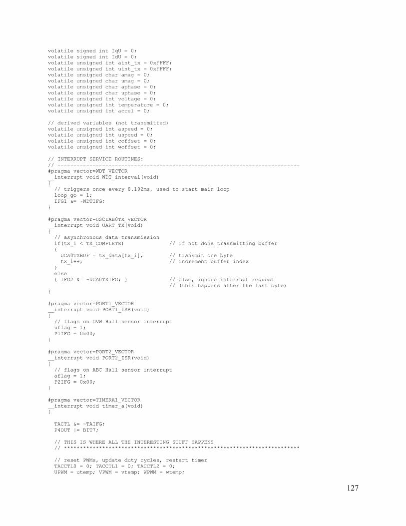
127

volatile signed int IqU = 0;volatile signed int IdU = 0;volatile unsigned int aint_tx = 0xFFFF;volatile unsigned int uint_tx = 0xFFFF;volatile unsigned char amag = 0;volatile unsigned char umag = 0;volatile unsigned char aphase = 0;volatile unsigned char uphase = 0;volatile unsigned int voltage = 0;volatile unsigned int temperature = 0;volatile unsigned int accel = 0;

// derived variables (not transmitted)volatile unsigned int aspeed = 0;volatile unsigned int uspeed = 0;volatile unsigned int coffset = 0;volatile unsigned int woffset = 0;

// INTERRUPT SERVICE ROUTINES:// ----------------------------------------------------------------------------#pragma vector=WDT_VECTOR __interrupt void WDT_interval(void){ // triggers once every 8.192ms, used to start main loop loop_go = 1; IFG1 &= ~WDTIFG;}

#pragma vector=USCIAB0TX_VECTOR__interrupt void UART_TX(void){ // asynchronous data transmission if(tx_i < TX_COMPLETE) // if not done trasnmitting buffer { UCA0TXBUF = tx_data[tx_i]; // transmit one byte tx_i++; // increment buffer index } else { IFG2 &= ~UCA0TXIFG; } // else, ignore interrupt request // (this happens after the last byte)}

#pragma vector=PORT1_VECTOR__interrupt void PORT1_ISR(void){ // flags on UVW Hall sensor interrupt uflag = 1; P1IFG = 0x00;}

#pragma vector=PORT2_VECTOR__interrupt void PORT2_ISR(void){ // flags on ABC Hall sensor interrupt aflag = 1; P2IFG = 0x00;}

#pragma vector=TIMERA1_VECTOR__interrupt void timer_a(void){

TACTL &= ~TAIFG; P4OUT |= BIT7; // THIS IS WHERE ALL THE INTERESTING STUFF HAPPENS // ************************************************************************** // reset PWMs, update duty cycles, restart timer TACCTL0 = 0; TACCTL1 = 0; TACCTL2 = 0; UPWM = utemp; VPWM = vtemp; WPWM = wtemp;

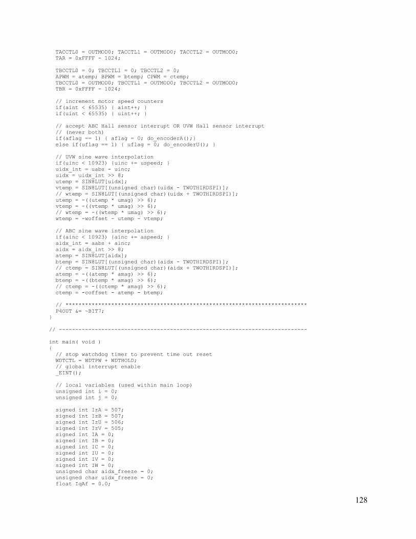
128

TACCTL0 = OUTMOD0; TACCTL1 = OUTMOD0; TACCTL2 = OUTMOD0; TAR = 0xFFFF - 1024; TBCCTL0 = 0; TBCCTL1 = 0; TBCCTL2 = 0; APWM = atemp; BPWM = btemp; CPWM = ctemp; TBCCTL0 = OUTMOD0; TBCCTL1 = OUTMOD0; TBCCTL2 = OUTMOD0; TBR = 0xFFFF - 1024; // increment motor speed counters if(aint < 65535) { aint++; } if(uint < 65535) { uint++; } // accept ABC Hall sensor interrupt OR UVW Hall sensor interrupt // (never both) if(aflag == 1) { aflag = 0; do_encoderA();} else if(uflag == 1) { uflag = 0; do_encoderU(); } // UVW sine wave interpolation if(uinc < 10923) {uinc += uspeed; } uidx_int = uabs - uinc; uidx = uidx_int >> 8; utemp = SIN8LUT[uidx]; vtemp = SIN8LUT[(unsigned char)(uidx - TWOTHIRDSPI)]; // wtemp = SIN8LUT[(unsigned char)(uidx + TWOTHIRDSPI)]; utemp = -((utemp * umag) >> 6); vtemp = -((vtemp * umag) >> 6); // wtemp = -((wtemp * umag) >> 6); wtemp = -woffset - utemp - vtemp; // ABC sine wave interpolation if(ainc < 10923) {ainc += aspeed; } aidx_int = aabs + ainc; aidx = aidx_int >> 8; atemp = SIN8LUT[aidx]; btemp = SIN8LUT[(unsigned char)(aidx - TWOTHIRDSPI)]; // ctemp = SIN8LUT[(unsigned char)(aidx + TWOTHIRDSPI)]; atemp = -((atemp * amag) >> 6); btemp = -((btemp * amag) >> 6); // ctemp = -((ctemp * amag) >> 6); ctemp = -coffset - atemp - btemp; // ************************************************************************** P4OUT &= ~BIT7;}

// ----------------------------------------------------------------------------

int main( void ){ // stop watchdog timer to prevent time out reset WDTCTL = WDTPW + WDTHOLD; // global interrupt enable _EINT(); // local variables (used within main loop) unsigned int i = 0; unsigned int j = 0; signed int IzA = 507; signed int IzB = 507; signed int IzU = 506; signed int IzV = 505; signed int IA = 0; signed int IB = 0; signed int IC = 0; signed int IU = 0; signed int IV = 0; signed int IW = 0; unsigned char aidx_freeze = 0; unsigned char uidx_freeze = 0; float IqAf = 0.0;

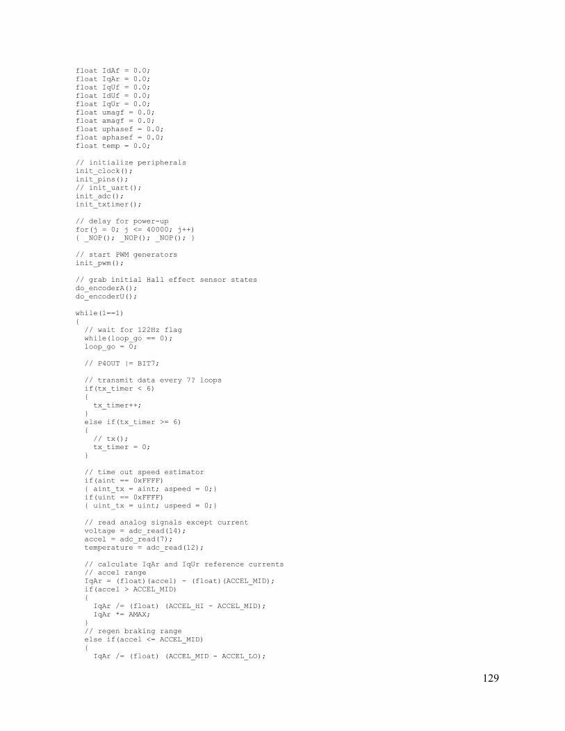
129

float IdAf = 0.0; float IqAr = 0.0; float IqUf = 0.0; float IdUf = 0.0; float IqUr = 0.0; float umagf = 0.0; float amagf = 0.0; float uphasef = 0.0; float aphasef = 0.0; float temp = 0.0; // initialize peripherals init_clock(); init_pins(); // init_uart(); init_adc(); init_txtimer(); // delay for power-up for(j = 0; j <= 40000; j++) { _NOP(); _NOP(); _NOP(); } // start PWM generators init_pwm(); // grab initial Hall effect sensor states do_encoderA(); do_encoderU(); while(1==1) { // wait for 122Hz flag while(loop_go == 0); loop_go = 0; // P4OUT |= BIT7; // transmit data every 7? loops if(tx_timer < 6) { tx_timer++; } else if(tx_timer >= 6) { // tx(); tx_timer = 0; } // time out speed estimator if(aint == 0xFFFF) { aint_tx = aint; aspeed = 0;} if(uint == 0xFFFF) { uint_tx = uint; uspeed = 0;} // read analog signals except current voltage = adc_read(14); accel = adc_read(7); temperature = adc_read(12); // calculate IqAr and IqUr reference currents // accel range IqAr = (float)(accel) - (float)(ACCEL_MID); if(accel > ACCEL_MID) { IqAr /= (float) (ACCEL_HI - ACCEL_MID); IqAr *= AMAX; } // regen braking range else if(accel <= ACCEL_MID) { IqAr /= (float) (ACCEL_MID - ACCEL_LO);

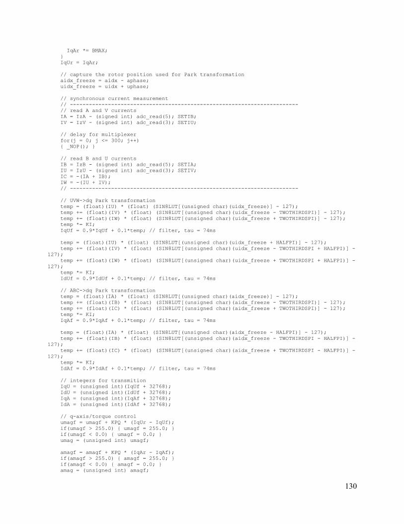
130

IqAr *= BMAX; } IqUr = IqAr; // capture the rotor position used for Park transformation aidx_freeze = aidx - aphase; uidx_freeze = uidx + uphase; // synchronous current measurement // ------------------------------------------------------------------------ // read A and V currents IA = IzA - (signed int) adc_read(5); SETIB; IV = IzV - (signed int) adc_read(3); SETIU; // delay for multiplexer for(j = 0; j <= 300; j++) { _NOP(); } // read B and U currents IB = IzB - (signed int) adc_read(5); SETIA; IU = IzU - (signed int) adc_read(3); SETIV; IC = -(IA + IB); IW = -(IU + IV); // ------------------------------------------------------------------------ // UVW->dq Park transformation temp = (float)(IU) * (float) (SIN8LUT[(unsigned char)(uidx_freeze)] - 127); temp += (float)(IV) * (float) (SIN8LUT[(unsigned char)(uidx_freeze - TWOTHIRDSPI)] - 127); temp += (float)(IW) * (float) (SIN8LUT[(unsigned char)(uidx_freeze + TWOTHIRDSPI)] - 127); temp *= KI; IqUf = 0.9*IqUf + 0.1*temp; // filter, tau = 74ms temp = (float)(IU) * (float) (SIN8LUT[(unsigned char)(uidx_freeze + HALFPI)] - 127); temp += (float)(IV) * (float) (SIN8LUT[(unsigned char)(uidx_freeze - TWOTHIRDSPI + HALFPI)] -127); temp += (float)(IW) * (float) (SIN8LUT[(unsigned char)(uidx_freeze + TWOTHIRDSPI + HALFPI)] -127); temp *= KI; IdUf = 0.9*IdUf + 0.1*temp; // filter, tau = 74ms // ABC->dq Park transformation temp = (float)(IA) * (float) (SIN8LUT[(unsigned char)(aidx_freeze)] - 127); temp += (float)(IB) * (float) (SIN8LUT[(unsigned char)(aidx_freeze - TWOTHIRDSPI)] - 127); temp += (float)(IC) * (float) (SIN8LUT[(unsigned char)(aidx_freeze + TWOTHIRDSPI)] - 127); temp *= KI; IqAf = 0.9*IqAf + 0.1*temp; // filter, tau = 74ms temp = (float)(IA) * (float) (SIN8LUT[(unsigned char)(aidx_freeze - HALFPI)] - 127); temp += (float)(IB) * (float) (SIN8LUT[(unsigned char)(aidx_freeze - TWOTHIRDSPI - HALFPI)] -127); temp += (float)(IC) * (float) (SIN8LUT[(unsigned char)(aidx_freeze + TWOTHIRDSPI - HALFPI)] -127); temp *= KI; IdAf = 0.9*IdAf + 0.1*temp; // filter, tau = 74ms // integers for transmition IqU = (unsigned int)(IqUf + 32768); IdU = (unsigned int)(IdUf + 32768); IqA = (unsigned int)(IqAf + 32768); IdA = (unsigned int)(IdAf + 32768); // q-axis/torque control umagf = umagf + KPQ * (IqUr - IqUf); if(umagf > 255.0) { umagf = 255.0; } if(umagf < 0.0) { umagf = 0.0; } umag = (unsigned int) umagf; amagf = amagf + KPQ * (IqAr - IqAf); if(amagf > 255.0) { amagf = 255.0; } if(amagf < 0.0) { amagf = 0.0; } amag = (unsigned int) amagf;

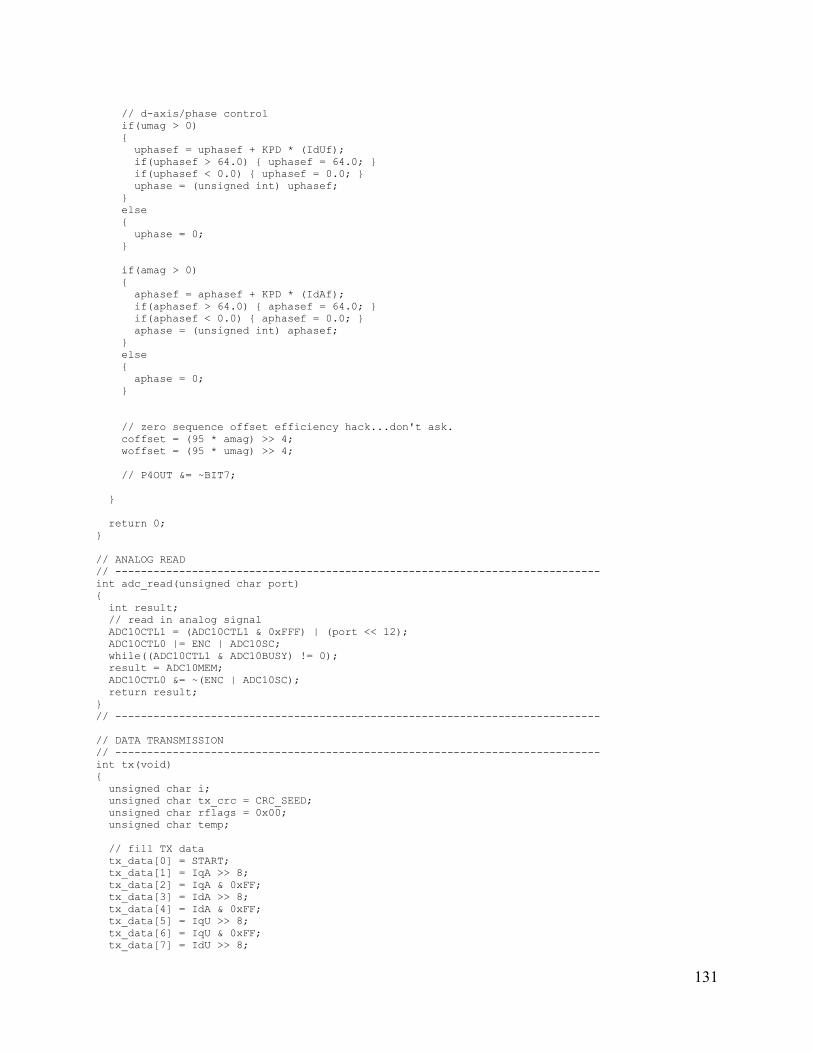
131

// d-axis/phase control if(umag > 0) { uphasef = uphasef + KPD * (IdUf); if(uphasef > 64.0) { uphasef = 64.0; } if(uphasef < 0.0) { uphasef = 0.0; } uphase = (unsigned int) uphasef; } else { uphase = 0; } if(amag > 0) { aphasef = aphasef + KPD * (IdAf); if(aphasef > 64.0) { aphasef = 64.0; } if(aphasef < 0.0) { aphasef = 0.0; } aphase = (unsigned int) aphasef; } else { aphase = 0; } // zero sequence offset efficiency hack...don't ask. coffset = (95 * amag) >> 4; woffset = (95 * umag) >> 4; // P4OUT &= ~BIT7; }

return 0;}

// ANALOG READ// ----------------------------------------------------------------------------int adc_read(unsigned char port){ int result; // read in analog signal ADC10CTL1 = (ADC10CTL1 & 0xFFF) | (port << 12); ADC10CTL0 |= ENC | ADC10SC; while((ADC10CTL1 & ADC10BUSY) != 0); result = ADC10MEM; ADC10CTL0 &= ~(ENC | ADC10SC); return result;}// ----------------------------------------------------------------------------

// DATA TRANSMISSION// ----------------------------------------------------------------------------int tx(void){ unsigned char i; unsigned char tx_crc = CRC_SEED; unsigned char rflags = 0x00; unsigned char temp; // fill TX data tx_data[0] = START; tx_data[1] = IqA >> 8; tx_data[2] = IqA & 0xFF; tx_data[3] = IdA >> 8; tx_data[4] = IdA & 0xFF; tx_data[5] = IqU >> 8; tx_data[6] = IqU & 0xFF; tx_data[7] = IdU >> 8;

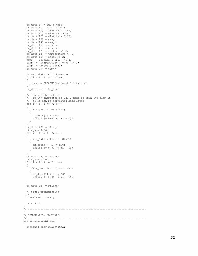
132

tx_data[8] = IdU & 0xFF; tx_data[9] = aint_tx >> 8; tx_data[10] = aint_tx & 0xFF; tx_data[11] = uint_tx >> 8; tx_data[12] = uint_tx & 0xFF; tx_data[13] = amag; tx_data[14] = umag; tx_data[15] = aphase; tx_data[16] = uphase; tx_data[17] = voltage >> 2; tx_data[18] = temperature >> 2; tx_data[19] = accel >> 2; temp = (voltage & 0x03) << 4; temp |= (temperature & 0x03) << 2; temp |= (accel & 0x03); tx_data[20] = temp; // calculate CRC (checksum) for(i = 1; i <= 20; i++) { tx_crc = CRC8LUT[tx_data[i] ^ tx_crc]; } tx_data[21] = tx_crc; // escape characters // (if any character is 0xFF, make it 0xFE and flag it // so it can be converted back later) for(i = 1; i <= 7; i++) { if(tx_data[i] == START) { tx_data[i] = ESC; rflags |= 0x01 << (i - 1); } } tx_data[22] = rflags; rflags = 0x00; for(i = 1; i <= 7; i++) { if(tx_data[7 + i] == START) { tx_data[7 + i] = ESC; rflags |= 0x01 << (i - 1); } } tx_data[23] = rflags; rflags = 0x00; for(i = 1; i <= 7; i++) { if(tx_data[14 + i] == START) { tx_data[14 + i] = ESC; rflags |= 0x01 << (i - 1); } } tx_data[24] = rflags; // begin transmission tx_i = 1; UCA0TXBUF = START; return 1;}// ----------------------------------------------------------------------------

// COMMUTATION ROUTINES:// ----------------------------------------------------------------------------int do_encoderA(void){ unsigned char grabstateA;

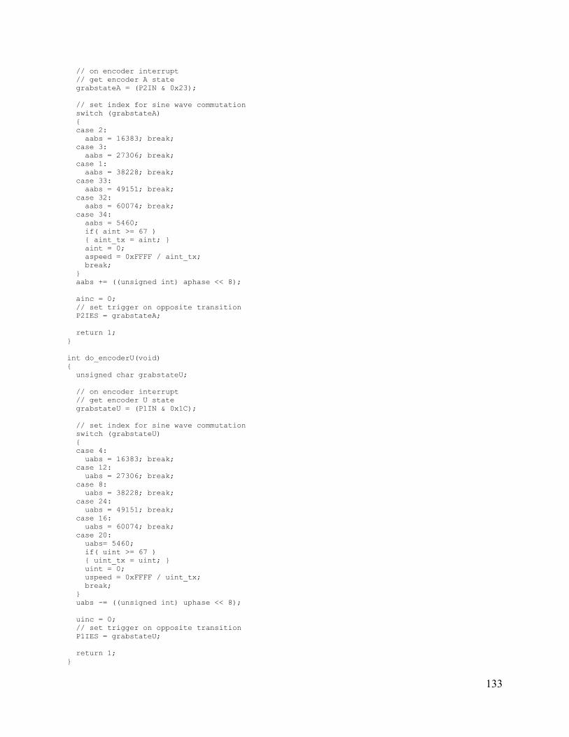
133

// on encoder interrupt // get encoder A state grabstateA = (P2IN & 0x23); // set index for sine wave commutation switch (grabstateA) { case 2: aabs = 16383; break; case 3: aabs = 27306; break; case 1: aabs = 38228; break; case 33: aabs = 49151; break; case 32: aabs = 60074; break; case 34: aabs = 5460; if( aint >= 67 ) { aint_tx = aint; } aint = 0; aspeed = 0xFFFF / aint_tx; break; } aabs += ((unsigned int) aphase << 8); ainc = 0; // set trigger on opposite transition P2IES = grabstateA; return 1;}

int do_encoderU(void){ unsigned char grabstateU; // on encoder interrupt // get encoder U state grabstateU = (P1IN & 0x1C); // set index for sine wave commutation switch (grabstateU) { case 4: uabs = 16383; break; case 12: uabs = 27306; break; case 8: uabs = 38228; break; case 24: uabs = 49151; break; case 16: uabs = 60074; break; case 20: uabs= 5460; if( uint >= 67 ) { uint_tx = uint; } uint = 0; uspeed = 0xFFFF / uint_tx; break; } uabs -= ((unsigned int) uphase << 8); uinc = 0; // set trigger on opposite transition P1IES = grabstateU; return 1;}

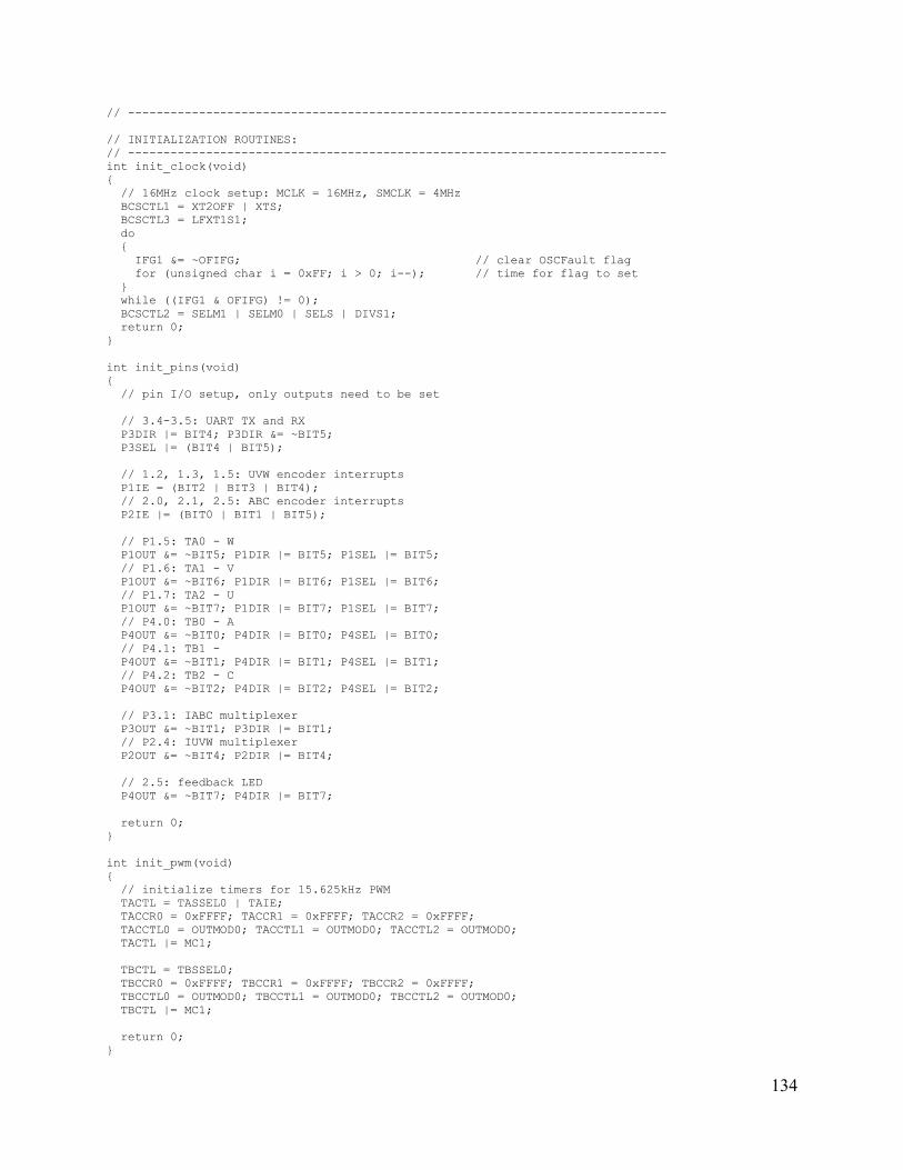
134

// ----------------------------------------------------------------------------

// INITIALIZATION ROUTINES:// ----------------------------------------------------------------------------int init_clock(void){ // 16MHz clock setup: MCLK = 16MHz, SMCLK = 4MHz BCSCTL1 = XT2OFF | XTS; BCSCTL3 = LFXT1S1; do { IFG1 &= ~OFIFG; // clear OSCFault flag for (unsigned char i = 0xFF; i > 0; i--); // time for flag to set } while ((IFG1 & OFIFG) != 0); BCSCTL2 = SELM1 | SELM0 | SELS | DIVS1; return 0;}

int init_pins(void){ // pin I/O setup, only outputs need to be set // 3.4-3.5: UART TX and RX P3DIR |= BIT4; P3DIR &= ~BIT5; P3SEL |= (BIT4 | BIT5); // 1.2, 1.3, 1.5: UVW encoder interrupts P1IE = (BIT2 | BIT3 | BIT4); // 2.0, 2.1, 2.5: ABC encoder interrupts P2IE |= (BIT0 | BIT1 | BIT5); // P1.5: TA0 - W P1OUT &= ~BIT5; P1DIR |= BIT5; P1SEL |= BIT5; // P1.6: TA1 - V P1OUT &= ~BIT6; P1DIR |= BIT6; P1SEL |= BIT6; // P1.7: TA2 - U P1OUT &= ~BIT7; P1DIR |= BIT7; P1SEL |= BIT7; // P4.0: TB0 - A P4OUT &= ~BIT0; P4DIR |= BIT0; P4SEL |= BIT0; // P4.1: TB1 - P4OUT &= ~BIT1; P4DIR |= BIT1; P4SEL |= BIT1; // P4.2: TB2 - C P4OUT &= ~BIT2; P4DIR |= BIT2; P4SEL |= BIT2; // P3.1: IABC multiplexer P3OUT &= ~BIT1; P3DIR |= BIT1; // P2.4: IUVW multiplexer P2OUT &= ~BIT4; P2DIR |= BIT4; // 2.5: feedback LED P4OUT &= ~BIT7; P4DIR |= BIT7; return 0;}

int init_pwm(void){ // initialize timers for 15.625kHz PWM TACTL = TASSEL0 | TAIE; TACCR0 = 0xFFFF; TACCR1 = 0xFFFF; TACCR2 = 0xFFFF; TACCTL0 = OUTMOD0; TACCTL1 = OUTMOD0; TACCTL2 = OUTMOD0; TACTL |= MC1; TBCTL = TBSSEL0; TBCCR0 = 0xFFFF; TBCCR1 = 0xFFFF; TBCCR2 = 0xFFFF; TBCCTL0 = OUTMOD0; TBCCTL1 = OUTMOD0; TBCCTL2 = OUTMOD0; TBCTL |= MC1; return 0;}

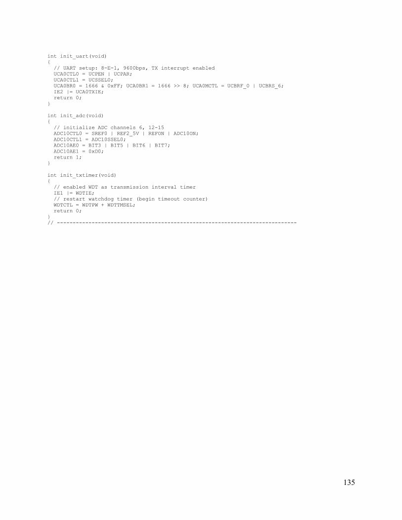
135

int init_uart(void){ // UART setup: 8-E-1, 9600bps, TX interrupt enabled UCA0CTL0 = UCPEN | UCPAR; UCA0CTL1 = UCSSEL0; UCA0BR0 = 1666 & 0xFF; UCA0BR1 = 1666 >> 8; UCA0MCTL = UCBRF_0 | UCBRS_6; IE2 |= UCA0TXIE; return 0;}

int init_adc(void){ // initialize ADC channels 6, 12-15 ADC10CTL0 = SREF0 | REF2_5V | REFON | ADC10ON; ADC10CTL1 = ADC10SSEL0; ADC10AE0 = BIT3 | BIT5 | BIT6 | BIT7; ADC10AE1 = 0xD0; return 1;}

int init_txtimer(void){ // enabled WDT as transmission interval timer IE1 |= WDTIE; // restart watchdog timer (begin timeout counter) WDTCTL = WDTPW + WDTTMSEL; return 0;}// ----------------------------------------------------------------------------