Embed Size (px)
Citation preview

i
DESIGN AND OPTIMIZATION OF MEMBRANE
FILTRATION AND ACTIVATED CARBON PROCESSES
FOR INDUSTRIAL WASTEWATER TREATMENT BASED
ON ADVANCED AND COMPREHENSIVE ANALYTICAL
CHARACTERISATION METHODOLOGIES
SALMAN ALIZADEH KORDKANDI, B.Sc., M.Sc.
A Thesis Submitted to the School of Graduate Studies in Partial Fulfilment
of the Requirements for the Degree Master of Applied Science
McMaster University © Copyright by Salman Alizadeh Kordkandi, August 2019

ii
MASTER OF APPLIED SCIENCE (2019) McMaster University
(Chemical Engineering) Hamilton, Ontario
TITLE: DESIGN AND OPTIMIZATION OF MEMBRANE FILTRATION
AND ACTIVATED CARBON PROCESSES FOR INDUSTRIAL
WASTEWATER TREATMENT BASED ON ADVANCED AND
COMPREHENSIVE ANALYTICAL CHARACTERISATION
METHODOLOGIES
AUTHOR: SALMAN ALIZADEH KORDKANDI, B.Sc. (UNIVERSITY
OF TABRIZ), M.Sc. (SAHAND UNIVERSITY OF TECHNOLOGY)
SUPERVISOR: Dr. DAVID LATULIPPE
NUMBER OF PAGES: 78

iii
Lay Abstract
Aevitas is an industrial wastewater treatment plant, which is situated at City of Brantford.
Every day, this plant receives about 15 trucks of mixture of wastewaters from many different
industries. The input wastewater into the plant should be treated and meet the environmental
standard so that it can be discharged into municipal wastewater plant. Currently, the
maximum allowable chemical oxygen demand (COD) for discharging the treated
wastewater from Aevitas to municipal wastewater treatment plant is 600 ppm. Despite the
fact, the current system in Aevitas is not efficient to meet this criterion. Thus, we strive to
design efficient processes to overcome the problem. To this end, 75 samples were collected
from Aevitas to observe the kind of chemicals that are the source of COD and then, two
processes including activated carbon adsorption and membrane filtration were used for
further reduction of COD. Although activated carbon can reduce the COD, the limited
adsorption capacity was a major concern for its long-term application, especially if the COD
of influent wastewater is higher than 2000 ppm. Membrane filtration was used as an
alternative for activated carbon and the results showed that membrane could reduce the
COD below 600 in the 48% of the cases.
iv
Abstract
Aevitas is an industrial wastewater treatment plant that receives about 300 m3/day of
mixture of wastewater from different industries. Chemical oxygen demand of higher 600
ppm and the variety of the chemical constitution of industrial wastewater are two significant
problems on Aevitas. Therefore, there is a strong need for developing advanced analytical
techniques that can identify the specific compounds that are the source of COD. During 10
months, about 75 industrial samples were characterised using a battery of tests including
GC/MS, COD, TOC, and pH to identify the chemicals that are main source of COD in the
industrial wastewaters. Results showed that the COD of 87% of 75 provided samples from
Aevitas plant were higher than 600.
At the first step of process design, activated carbon was used to eliminate the identified
organic chemicals from the wastewaters. The maximum and minimum of COD removal
(depends on the chemical composition) of the wastewaters were obtained as 94 and 24%,
respectively. Moreover, the amount of COD and TOC that can be adsorbed on the surface
of 1 gram of the activated carbon were 25 and 7 mg, respectively. Although activated carbon
is capable to reduce the COD, its capacity of adsorption is limited. To overcome this
problem an alternative process, membrane filtration was applied for COD removal.
Two types of crossflow NF (NF270, NF90, NFX, NFW, NFS, TS80, XN45, and
SXN2_L) and RO (BW60 and TW30) membranes in two modules of spiral wound and
flat sheet were used. The filtration results of 11 different industrial wastewaters showed
that NF90, TS80, NFX, and NFS were effective in COD removal. However, in terms of
output flux NFX and NFS flat sheet were better than others were. Similar to the activated
carbon process, the COD removal in filtration process was between 30 and 90%. The
obtained results can be used to scale up the membrane filtration process at Aevitas.

v
Acknowledgment
I would like to thank my supervisor Dr. David Latulippe for his supports and advises in
many aspects like presenting data, meetings, and providing samples from Aevitas Inc. as
well as his management in conducting the project.
I am grateful to my industrial partner at Aevitas Inc. for my funding, especially those who
have helped and advised me, principally Tom Maxwell, Milos Stanisavlvjevic, Jo-ann
Livingston, and Richard Mock.
I am particularly indebted to Dr. Mehdi Zolfaghari (for many great discussions on
wastewater treatment), Patrick Morkus (for collaboration, services, and spiritually support),
Dr. Amirsadegh Kazemi, Indranil Sarkar, Abhishek Premachandra, Jacob Sitko (helping me
for conducting part of experiments), and Ryan LaRue.
I also need to thank those at DOW Inc. for providing membranes, McMaster Regional
Centre for Mass Spectrometry (MRCMS), Dr. Kirk Green, and Dr. Fan Fei for sample
analysis, Dr. Shiping Zhu's Lab for their help in sample preparation.
It is my pleasure to thank Professor Carlos Filipe for his spiritually support and accepting
my invitation for being one of my committee member and finally thanks to Dr. Charles de
Lannoy the other committee member!
At the end, I would like to appreciate the Natural Sciences and Engineering Research
Council of Canada (NSERC) for supporting this project.
vi
Table of Contents
Introduction and Background ........................................................................................ 1
1.1. Single source industrial wastewater properties ......................................................... 2
1.2. Multi-source time-varying industrial wastewater properties .................................... 7
1.3. Motivation and objective of the project ..................................................................... 9
Materials and Methods .................................................................................................. 12
2.1. Sampling from Aevitas facility ................................................................................. 12
2.2. Analytical procedures .............................................................................................. 13
2.2.1. Sample preparation and GC/MS analysis ............................................................ 13
2.2.2. LC/MS/MS analysis ............................................................................................. 15
2.2.3. COD measurement ............................................................................................... 15
2.2.4. TOC measurement ............................................................................................... 16
2.2.5. pH and conductivity measurement....................................................................... 17
2.2.6. Turbidity measurement ........................................................................................ 17
2.3. Experimental Set up ................................................................................................. 18
2.3.1. Batch and Rapid Small Scale Column Test ......................................................... 18
2.3.2. Pressure driven membrane filtration and the types of used membranes .............. 19
Results and Discussion ................................................................................................... 23
3.1. Identifications and occurrences of organic chemicals in industrial wastewater .... 24
3.2. Adsorption of organic chemicals during Activated Carbon Process....................... 27
3.2.1. Batch Process Activated Carbon Adsorption ....................................................... 27
3.2.2. Sequential Activated Carbon Adsorption ............................................................ 30

vii
3.3. Pressure-driven membrane filtration for separation of organic chemicals from
wastewater ........................................................................................................................... 33
3.3.1. COD removal from wastewater using different membranes ............................... 35
3.3.2. Membrane filtration COD removal versus flux ................................................... 39
3.4. Sequential membrane filtration followed by activated carbon process ................... 41
3.5. Process modelling .................................................................................................... 44
3.5.1. Principal Component Analysis ............................................................................ 45
3.5.2. Variation in Sampling, and outliers ..................................................................... 46
3.5.3. Most Significant Process’s Parameters and Chemicals in Wastewater before and
after treatment using activated carbon ............................................................................. 48
3.5.4. Artificial Neural Network .................................................................................... 53
3.5.5. Process performance prediction by definition of water quality using ANN ........ 55
Conclusions ..................................................................................................................... 57
Recommendations for future works ............................................................................. 60
References ....................................................................................................................... 62

viii
List of Table
Table 1. Characteristic of food industrial wastewater [9]. ......................................................... 4
Table 2. Characteristic of seven textile wastewaters which have been used for manufacturing
different types of textile material [18]................................................................................. 6
Table 3. Characteristic of a typical chemical manufacturing wastewater containing a wide range
of organic chemicals[1, 26]. ................................................................................................ 8
Table 4. Properties of RO and NF membrane used in the experiment. ................................... 22
Table 5.The chemicals with high occurrences in Aevitas wastewater. These chemical are the
results of 150 samples, which 75 of them were before treatment and 75 were after
treatment. ........................................................................................................................... 24
Table 6. ANOVA table for the experiments using BW9. ........................................................ 36
Table 7. Removal percentage of chemicals from BW9 using NF90 and NFW in according to
Fig. 12................................................................................................................................ 38
Table 8. The R2 and Q2 of the PCA modelling when more seven components were used; as the
number of components increases the model will be more accurate. ................................. 49
List of Figures
Figure 1. Schematic diagram of Aevitas industrial wastewater treatment plant...................... 10
Figure 2. The pressure driven NF and RO membrane set up applied for wastewater treatment
in two flat sheet and spiral wound modules. ..................................................................... 21
Figure 3. SEPA cell pictures for testing flat sheet membranes (A) and the spiral wound 1812
module (B) that were used for industrial wastewater treatment. ....................................... 21

ix
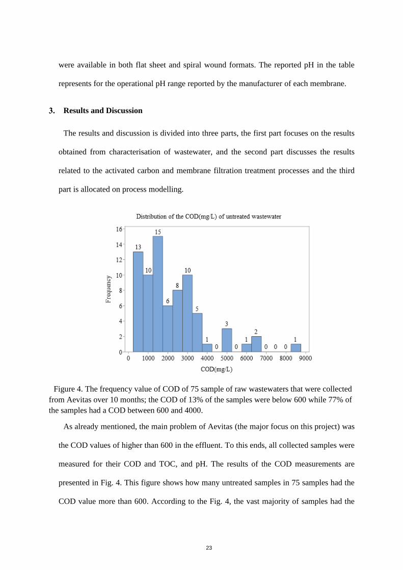
Figure 4. The frequency value of COD of 75 sample of raw wastewaters that were collected
from Aevitas over 10 months; the COD of 13% of the samples were below 600 while 77%
of the samples had a COD between 600 and 4000. ........................................................... 23
Figure 5. GC/MS spectrum of four industrial samples received from Aevitas; A) ED42,
COD=4970 with 18 sharp peaks (67% known + 33% unknown); B) ED52, COD=720 with
41 sharp peaks (29% known + 71% unknown) C) ED65, COD=974 with 17 sharp peaks
(59% known + 41% unknown); D) ED68, COD=6172 with 9 sharp peaks (89% known +
11% unknown). There is a positive correlation between the COD values and maximum
intensity of the peaks (for spectrum (D) is 4.5×10⁻⁷ while for spectrum (B) is below 0.1×10-
7). ....................................................................................................................................... 27
Figure 6. Treatment of the collected samples from Aevitas using activated carbon adsorption;
the empty redline and the full blue bars are the amount of COD at the time before adding
activated carbon and at the end of experiment, respectively. The applied amount of applied
activated carbon for each experiment depends on the amount of their TOC were kept
constant (1-gram activated carbon per 10 mg of TOC). ................................................... 29
Figure 7. The full GC/MS spectrum of two samples (ED42 (A) and ED68 (B)) before treatment
(redline) and after treatment (blue line) using activated carbon. Activated carbon
successfully adsorbed all the detectable chemicals by GC/MS from wastewater and thus
the COD values decreased................................................................................................. 30
Figure 8. Sequential adsorption of organic chemicals from BW7 (diluted) and BW8 on the
surface of activated carbon (continental carbon group); initial COD of BW7 (diluted) and
BW8 were 2016 and 748, respectively; initial activate carbon in BW7 and 8 were 5.33 and
1.8 gram, respectively. The COD removal at the second stage was significantly lower than
the first stage of adsorption. .............................................................................................. 31
x
Figure 9. The result of Rapid Small-Scale Column Tests using BW2, and BW3 with influent
TOC of 383 (COD of 1264) and 1180 (COD of 4400), respectively. The breakthrough
curve is observed around 10 minutes in both conditions which means activated carbon
column cannot tolerate even at TOC of 383 ppm (or COD of ~1264) ............................. 32
Figure 10. A comparison between two typical industrial wastewater (BW11 and 12) in terms
of the amount of the suspended solid and their permeate after filtration by NF90. .......... 34
Figure 11. The concentration of COD in the permeate of BW9 (diluted) after using different
NF membranes filtration; the input feed corresponds to the blue bar has been diluted 4
times(75% tap water + 25% wastewater) whereas the empty bars was the result of one time
dilution (50% tap water + 50% wastewater) from the original wastewater. NF90 had a
highest COD removal of 64%, but none of them reduced the COD below 600. .............. 37
Figure 12. Comparison of GC spectrum of untreated BW9 (at the top), treated using NF90 (the
middle) and NFW (at the bottom). While NF90 successfully removed all the peaks in the
untreated sample, there was some chemicals remained in the NFW permeate................. 37
Figure 13. COD removal of three different wastewaters three wastewater BW10 (COD: 1100),
BW11 (COD: 1100), and BW12 (diluted COD: 1700), BW12 (COD: 4200) using NFX,
TS80, and NF90 flat sheet NF membranes. NF90 had a better performnce than others did.
........................................................................................................................................... 39
Figure 14. Flux of three different flat sheet NF membranes; NFX, TS80, and NF90, which were
used for treating three wastewater BW10 (COD: 1100), BW11 (COD: 1100), and BW12
(diluted COD: 1700), BW12 (COD: 4200), NFX had a better flux than others did. ........ 41
Figure 15. Sequential membrane (RO and NFs)-activated carbon treatment of wastewater
(BW7) containing organic chemicals using. BW7 with original COD of 8400 was diluted

xi
for being used as an actual feed with a normal COD. Membrane filtration as first step had
a great contribution in COD removal. ............................................................................... 43
Figure 16. GC/MS spectrum of diluted BW7 when being treated by sequential membrane (NFX
spiral wound)-activated carbon process. The COD of the feed, permeate, and treated
permeate by activated carbon were, 1315, 511, and 475, respectively. Membrane filtration
reduced the peaks considerably, while, the influence of activate carbon was not significant.
........................................................................................................................................... 43
Figure 17. Squared Prediction Error to show and eliminate the wastewater (with code EDxx)
that indicates abnormal properties; according to SPE, three data were ignored as they were
outliers. .............................................................................................................................. 47
Figure 18. T2 Hoteling statistic for outliers to show and eliminate the wastewater (with code
EDxx) that indicates abnormal properties; according to HT2, three data were ignored as
they were outliers. ............................................................................................................. 48
Figure 19. T Score plot for PCA model. Untreated sample were placed in the right hand side
and after treatment by activated carbon they shifted into left hand side; this helps to see if
a conducted experiment was abnormal or the characteristic of sample before/after treatment
was abnormal..................................................................................................................... 50
Figure 20. Loading plot: the relationship between all the variables used to build PCA model
and shows which variable had the most similar influence in building the model. ............ 51
Figure 21. Contribution plot of the PCA model based on the applied variables. This shows the
magnitude of the variation of each variable. The variation in RT-6-8 was the highest, which
means using activated carbon can remove all the peaks appeared between 6 and 8 min in
untreated sample. ............................................................................................................... 52

xii
Figure 22. The calculated MSE for Train, Validation, and Test stages of the dataset (obtained
from measuring the properties of wastewater before and after treatment using activated
carbon). .............................................................................................................................. 54
Figure 23. Architecture of the built ANN model; 11 variables were considered as input of 649
data and the same number of variables were predicted based on the input; hidden layer is
non-linear and the output layer is linear. ........................................................................... 55
Figure 24. Performances of the ANN in prediction quality of industrial wastewater treated by
activated carbon; the obtained MSE for building the model was ~10-4 and the R2 was 0.68.
It means this model can predict the quality of 68% of wastewater with confidence interval
of 0.95................................................................................................................................ 56

1
Introduction and Background
In any kind of wastewater treatment, two methods of handling are used for processing the
pollutants, one is water in liquid form, (which is the main constituent of the wastewater) and
the other method is attributed to the solid part or the sludge which has been dispensed in the
water. In addition, there are several kinds of wastewater including municipal wastewater
(i.e. from schools, offices, residential buildings, and so forth), industrial wastewater (i.e.
textile, brewery, leather, automotive, and so forth), and storm water (i.e. rainwater) [1]. The
wastewaters must be treated before being discharged to the natural environment for several
reasons [2]:
To prevent suspended solid from discharge back to the natural environment.
To prevent aquatic system and wildlife from potential hazardous chemicals.
Human health concern.
To recycle the water for the matter of water scarcity.
The wastewater must be characterized before choosing the treatment technique. Generally,
three categories of characterization, physical (i.e. color, odor, temperature, turbidity and so
on), chemical (i.e. organic compounds, nutrients and dissolved solids), and biological (i.e.
bacteria, viruses, and parasites) are investigated. High amount of organic carbon is one of
the major concern that has been at the center of attention due to the cause of oxygen
depletion in aquatic system. The organic compounds that are existed in the industrial
wastewater have some common and significant properties:
Some of them are combustible.
Their boiling or melting points are not high
Less soluble in water
Are available in high molecular weight (Mw)
2
Almost forms the main component of food for aquatic existents.
There are several sources for production of organic chemicals, natural (i.e. vegetable,
natural oil, cellulose, and starch), synthetic (plastic, rubber, and polymer), and
biotechnology (alcohols, antibiotic, and organic acid). When the organic compounds are
discharged into the environment, depending on their physiochemical properties, different
rates of degradation are observed. Microorganisms can easily degrade organic compounds
like alcohol, organic acid, and starch. However, on the other hands, non-biodegradable
organic compounds like Polycyclic Aromatic Hydrocarbons (PAHs) have a toxic effect on
aquatic system in some cases where it has been exposed to the microorganism. Since the
treatment of the PAHs (i.e. biocide, industrial waste, cellulose, and phenol) is difficult in
the natural environment, they stay in ecosystem for a long time. Increasing the amount of
organic compounds in water carries many undesirable effects on ecosystem. For example,
producing Trihalomethane (a carcinogenic chemical) as a result of oxygen depletion can be
occurred at high concentration of organic matter in water. Although the amount of total
organic carbon (TOC) can be measured accurately by TOC analyzer as a parameter for
defining the quality of water, two other criteria named Chemical Oxygen Demand (COD)
and Biochemical Oxygen Demand (BOD) are also common to express the quality of water
too. However, most of the industrial wastewaters contain toxic chemicals, and thus BOD
cannot be a proper criterion to express the quality of the effluent.
1.1. Single source industrial wastewater properties
Despite the fact that Canada is one of the most successful countries in waste reclamation,
about 411 million litres of wastewater still needs to be treated before being discharged to
the natural environment [3]. The standard for discharging an industrial wastewater depends
upon the guidelines endorsed by the regional government or local cities. Factors influencing

3
these rules are the availability of the water source and the infrastructure for shipping of the
wastewater into the treatment plant. The quantity and quality of the industrial wastewater
depend on the industries that produce the wastewater. Mining, food, petroleum, pigment,
beverage, pulp and paper, tanning, oil, and textile industries can be considered as the main
sources of wastewater in Canada [4]. In most cases, organic matter makes up to 70% of the
solid portion of wastewater.
For example, in food industry, several processes are used to produce the final product and
the type of products affects the composition of output wastewater from this industry.
Although the applied processes can influence the final product, there are some common
features among the wastewater from food industries [5] which have been listed as below:
High amounts of proteins and fats and carbohydrates[6]
A bioprocess can be used to eliminate the organic matters and the nitrogen
simultaneously [7]
Most of the time, the ratio of the main substrate such as carbon, nitrogen, and
phosphorous is not balanced for biodegradation processes [8]. For example, the
wastewater from potato processing industry contains high amount of starch, which is
an added source of organic carbon. For biodegradation of the organic carbon by
bacteria, sources of phosphorous and nitrogen should be added to the bioprocess to keep
the treatment efficient.
The wastewater from food industries are the output of three main applications; 1)
transportation, 2) cleaning, and 3) processing. To treat these industrial wastewaters several
consecutive processes including sedimentation, flocculation, coagulation, and oxidation are
needed to reduce the COD to an acceptable level. For example, to treat wastewater from

4
slaughterhouse or French fries processing, a grease separation from the water can be of great
help for the next treatment steps. In addition, in the brewery industry, most of the volume
of the water is spent on the cleaning of the barley and usually every 100 kg of barley produce
about 700 litre of wastewater, which contains both fibres, minerals, and proteins. Although
the composition of an industrial food wastewater is non-toxic, its volume and COD is
relatively high [9]. The following table is provided to show the characteristics of an
industrial food wastewater. Several papers published their results regarding the industrial
food wastewater treatment.
Table 1. Characteristic of food industrial wastewater [10].
Industry TS (ppm) TP
(ppm)
TN
(ppm)
BOD
(ppm)
COD
(ppm)
Flour and
Soybean - 3 50 600-4000 1000-8000
Palm oil mill 40 - 750 25 50
Sugar-beet
processing 6100 2.7 10 - 6600
Dairy 1100-1600 - - 800-1000 1400-2500
Corn milling 650 125 174 300 4850
Potato chips 5000 100 250 5000 6000
Baker’s yeast 600 3 275 - 6100
Winery 150-200 40-60 310-410 - 18000-
21000
Dairy 250-2750 - 10-90 650-6250 400-15200
Cheese dairy 1600-3900 60-100 400-700 - 23000-
40000
Olive mill 75500 60-100 400-700 - 130100
Cassava starch 830 90 525 6300 10500

5
For example, in a study conducted by Béatrice, reverse osmosis (RO) membrane has been
used for treating dairy industry wastewater [11]. For tracking the treatment efficiency of the
RO process, two parameters, TOC, and conductivity of the samples were measured. The
calculation of their results indicated that 540 m2 of RO membrane is required to treat 100
m3 of wastewater per day with 95% water recovery [11]. Membrane processing technology
with a flux of around 11 Lh−1 m−2 was used for the treatment of that wastewater and the
content of TOC in the permeate sample of the filtration was measured as 7 ppm while the
conductivity dropped down to 50 μScm−1 [12].
Automotive industry is another industry that needs high volume of water. The water in this
industry is used for rinsing different parts of the cars which need to be coated or finished
[13]. These type of wastewaters contain high amounts of oil and grease[14], hence, the
concentration of the organic chemicals in the wastewater is high, especially oily-based
compounds. The oil generally forms an unstable emulsion, oily wastewater emulsion or a
totally immiscible mixture [15]. While the oil content can be separated from an immiscible
mixture or unstable emulsion by physiochemical treatments, the oily wastewater emulsion
cannot be easily separated using conventional techniques due to the presence of surfactants,
which form a solution/emulsion with very small drops in micro size. In an effort made by
Bo Lai et.al coagulation-flocculation process was used for COD removal from automobile
manufacturing industrial wastewater [16]. The initial COD of 1222 was undergone
treatment process and after 30 min of reaction the COD dropped down to about 120 [16].
An ultrafiltration flat sheet membrane has been used for metal, COD, and BOD removal
from automobile manufacturing wastewater [17].
The wastewater from textile and dye manufacturing industries have different influences
on natural environment. Since several processes (i.e. wool and cotton) are involved in fibre

6
finishing and preparation, a variety of compounds are expected to be in the wastewater. The
important sources of pollution in textile wastewater are from scouring, mercerizing,
bleaching, dyeing, printing, and carbonization. Some of the produced pollutants during the
process are toxic and some of them damage the environment aesthetic. Analysis of the
composition of textile wastewater showed that the main cause of colour in the wastewater
are some azo bond, aniline, hydroquinone and naphthol chemicals, which are fluorescent
organic compounds. The following Table shows the characterisation of dying wastewater
that have been taken from seven different industries.
Table 2. Characteristic of seven textile wastewaters which have been used for
manufacturing different types of textile material [18].
Long Wu et.al made an effort to modify activated carbon via non-thermal plasma to
improve the adsorption of cupric ions [19]. The results revealed that adsorption capacity of
modified activated carbon improved by 150% relative to the pristine activated carbon [19].
In another work the bamboo based activated carbon has been synthesized for adsorption of
phenol and pharmaceuticals with the amine-functionalized magnetic group [20]. In a study
by Tawfik et. al. a developed model on phenol adsorption process showed that the maximum
Parameters Category
1 2 3 4 5 6 7
BOD5/COD 0.2 0.29 0.35 0.54 0.35 0.3 0.31
BOD5 (ppm) 6000 300 350 650 350 300 250
COD (ppm) 8000 1040 1000 1200 1000 1000 800
Oil and Grease
(ppm) 5500 - - 14 53 - -
TSS (ppm) 8000 130 200 300 300 120 75
Phenol (ppm) 1.5 0.5 - 0.04 0.24 0.13 0.12
Colour (ADMI) 2000 1000 - 325 400 600 600
PH 8 7 10 10 8 8 11
Temp. (°C) 28 62 21 37 39 20 38
Water usage (1 kg-
1) 36 33 13 113 150 69 150

7
adsorption capacity of activated carbon was 18.12 mg per gram of activated carbon modified
by diethylenetriamine [21].
In steel and iron wastewater treatment process a significant amount of acid, dust, oil and
grease should be removed as the casting in blast furnaces involves these pollutants [22].
During the finishing process coke ovens needs the most volume of the water for cooling
down the temperature of hot coke and the oven. Normally 0.4 L of water is need to produce
1 kg of coke, however, many toxic contaminants including cyanides, ammonia, phenol, and
thiocyanate will be added into the water. Although the amount of soluble COD is not a
matter of concern in this wastewater, the concentration of very toxic chemicals is higher
than the standard range.
1.2. Multi-source time-varying industrial wastewater properties
As mentioned in the previous section most of the works that have been done in this area
are the industrial wastewater treatment from only one source of wastewater production and
the pollutants in them are somehow predictable. While the challenges of multi-sources
industrial wastewater treatment is the introducing a versatile technique to remove the high
amount chemical pollutants so that the wastewater (after treatment) can be discharged into
municipal wastewater treatment plant. Principally, there are two options for eliminating
these pollutants, first one is using on-site treatment package and the other one is shipping
the wastewater from industrial site to a central plant for further treatment [1]. Each option
has its merits and demerits, however, offsite treatment owing to the low cost of facility
establishment in terms of the volume of the wastewater being treated, planning, and
operations are more favourable for multi-source industrial wastewater treatment [23]. The
difficult task is to find the best match treatment for each wastewater with a different
chemical composition. To construct an effective treatment plant, a comprehensive

8
characterisation of input industrial wastewater is significant. Knowing the source of the
wastewater is helpful to have an idea about the majority of the chemicals that have been
released in the output wastewater from industries, however, for some reasons the
information from all industries is not available [24, 25]. In such occasions, a comprehensive
analytical method should be developed to clarify the composition of the mixture. Mixing
different wastewaters also needs a high level of safety as some chemicals might react when
they are mixed. To assess and reduce the risk of any undesirable action, those industries that
are potential to produce hazardous or explosive chemicals should be determined and their
wastewater should be carried via different trucks. The produced wastewater from organic
chemical manufacturing plant could be a good example for mixture of different wastewater
as it includes many chemicals.
Table 3. Characteristic of a typical chemical manufacturing wastewater containing a wide
range of organic chemicals[1, 26].
Product BOD (ppm) COD (ppm) TSS (ppm)
Phthalic acid anhydride and maleic
acid anhydride - 150-300 20-50
Methyl acrylate acid - 7000-12000
6000-
12000
Butadiene and styrene 4000-8000 2000-3200 50-100
Isocyanates 300-600 900-1600 200-500
Acrylates 1000-2000 800-1500 20-40
Ethylene and propylene 400-600 800-1200 40-75
Methyl and ethyl parathion 2000- 3500 4000-6000 50-100
Acrylic nitrile 200-500 600-1200 80-150
Raw materials for the pigment
industry 200-400 1000-2000 80-200
Esters 5000-12000 10000-20000 20-100
Organic acids 300-600 40000-60000 150-300
Ketones
10000-
20000 5000-15000 100- 200
Acetaldehyde
15000-
25000 20000-40000 50-100
Organic phosphate compounds 500-1000 1500-3000 200-400

9
Usually, water in complex chemical industries is used for cooling, transportation of waste,
raw material, and solvent. The following table represents typical characteristics of a
chemical manufacturing wastewater. In 2011, Bianco et .al used Fenton process for treating
complex wastewater. They consider COD removal as a criterion for the effectiveness of the
process [27] and on average 80% of the COD has been removed from the complex
wastewater. In another attempt that was intended to treat the mixture of different industrial
wastewaters from foodstuff, dye house, refinery, electrochemical, and chemical industries,
an RO system is used for separation of wide range of contaminants [28]. In a similar case a
Nanofiltration integrated with forward osmosis was applied to reduce COD from mixture of
different wastewaters and at the transmembrane pressure of 12 bar a chemical removal of
99% was obtained [29]. Moreover, Marko showed that NF90 could remove more than 70%
of dissolved organic carbon from rendering plant wastewater [30].
1.3. Motivation and objective of the project
As mentioned in the introduction and background sections, some general reasons have
been given for why industrial wastewater should be treated, and as this is an important
ecological and economical issue, the governments of Canada and Ontario put a new strict
standard on the effluent quality. The Wastewater Systems Effluent Regulations (WSER),
which were established by the federal Fisheries Act in 2012 and came into force in 2015,
are a new set of national effluent quality standards. The first compliance deadline for ‘high
risk facilities’ to meet the WSER criteria is December 2020 and thus there is a pressing need
for improved treatment technologies for industrial wastewater sources. One of these
facilities is Aevitas that works on industrial wastewater treatment and the plant is situated
at City of Brantford, Ontario. This plant is an off-site wastewater treatment plant and
receives about 300 m3 (on average) of mixture of different industrial wastewaters from

10
several industries every day. To treat this volume of wastewater by meeting the standard
criteria, Aevitas is applying several consecutive processes. According to Fig. 1, the mixture
of industrial wastewater is shipped out from industrial plants to Aevitas for treatment and at
the end of the treatment processes; it has been discharged into the municipal wastewater
treatment plant. At the first stage, the received industrial wastewater is collected in an
equalization tank for primary tests and if it is possible to be treated in the plant the
wastewater then goes through the system, which is flocculation. After giving enough time
for settling the formed floc, aeration and oxidation using Fenton-like process are the next
processes for separation of supernatant.
Figure 1. Schematic diagram of Aevitas industrial wastewater treatment plant.
The remained organic chemicals that are not being separated in the flocculation stage
would be oxidize and volatilize in this stage of treatment. After these two main stages, the
majority of COD is removed from the wastewater and then a sample is taken at the end of
aeration/oxidation to see if the level of COD meets the environmental standards. Most of
the times the effluent COD of this point of plant is higher than 600 (a concentration that
City of Brantford enact for a safe discharging of the industrial effluent into the municipal

11
wastewater treatment plant) and thus needs further treatment to get the regulatory
compliance requirements. Although the level of COD is one part of the problem for
discharging the treated industrial wastewater into the municipal wastewater treatment plant,
the presence of biocides even at low concentrations can be harmful for bacteria that are
responsible for biodegradation.
Regarding these two aspects, at first step of work, a GC/MS-based characterisation
technique was developed to capture the most organic chemicals that were the source of COD
in the wastewater. Given the variety in composition of industrial wastewater from different
sources, the conventional ‘bulk measurements’ of organic contaminants, such as chemical
oxygen demand (COD) or total organic carbon (TOC) are not suitable. Thus, there was a
strong need for advanced analytical techniques that can identify and quantify the specific
compounds that were present in industrial wastewater sources. For this reason, a library of
the identified chemicals was built to monitor the occurrence of each chemical in the
wastewater treated by aeration/oxidation. As for the wastewater treatment technique,
activated carbon in two modes of flow, batch and continues (column), were used to
overcome the two problems. The experimental results showed that the activated carbon is
effective in both COD and biocide removal and, the cost of the removed COD per used
activated carbon is high. This might be because of the limited capacity of activated carbon
in adsorption process. To improve the polishing capacity, an alternative has been applied
which was a membrane-based separation technique. A pressure-driven membrane filtration
was used instead of activated carbon to reduce the spent cost as well as improving the
effectiveness of the treatment process. The experimental results showed that membrane
could be highly efficient in COD removal in most of the cases so that the environmental
criteria is met.

12
Materials and Methods
2.1. Sampling from Aevitas facility
Taking sample from industrial wastewater treatment plant is a crucial step for obtaining a
reliable and inclusive data. The type and the time of sampling highly depends upon the mode
of the applied flow in the plant. Thus, the operators should be aware of the discharging
procedure so that proper samples can be taken from which valuable information can be
obtained [4]. The other things that operator must take into account is the standard criteria
that the effluent should be discharged by low. This helps, as it tells us if the average
concentration of a particular compound or bulk concentration of a wastewater (i.e. COD or
BOD) at a particular time should be controlled. Moreover, the trend of the concentration
should be monitored as well as the source of the wastewater that come into the plant. The
concentration trend for a long time, which shows the fluctuation of COD, can be used where
several times of sampling for decreasing the uncertainty is uneconomical.
Since the mode of flow in Aevitas plant is batch process, the samples are collected after
each new batch to characterise the chemical composition of new wastewater sample. The
samples were collected in 1L of bottle and then was received at McMaster University for
further analytical tests. The collected samples in the bottle were stored in a 4 oC fridge to
prevent changes in sample composition. The wastewater samples collected from Aevitas
plant were based on two plans, A and B.
During plan A, about 75 samples in a 1L bottle were collected for characterisation. These
samples were called ED01, ED02, ED03, …, ED75, which the ED stands for effluent
discharged and the following number is showing the order of samples that received at
McMaster University. The same samples were used for treatment in the batch activated
13
carbon process and the sample after treatment were used for characterisation as well to
observe the kind of organic chemicals that have been adsorbed on the activated carbon.
During plan B, 11 wastewaters which called BW1, BW2, …, BW11 with volume of 20 L
were received from Aevitas and 2 of these samples were used for the activated carbon
column test and 9 of them were used for membrane filtration experiments. The chemical
composition of each wastewater was different. Similarly, samples were taken from these
experimental runs before and after treatment using activated carbon column and membrane
filtration for analysing the variation in chemical composition.
2.2. Analytical procedures
2.2.1. Sample preparation and GC/MS analysis
A 100 mL aliquot of each industrial WW sample was pH-adjusted to 2.0 ± 0.2 via the
addition of 1N HCl solution (LabChem), then combined with 100 mL of dichloromethane
(DCM) (Caledon) in a separatory funnel and manually shaken for one minute. The resulting
mixture was allowed to rest for five minutes in order to partition into two separate phases.
Approximately 100 mL of the bottom DCM rich phase was extracted from the separatory
funnel and then dehydrated by pouring it through approximately 5g of anhydrous sodium
sulfate (Anachemia) contained on top of a 30 µm Whatman filter paper in a simple glass
funnel. The dehydrated and filtered sample was then concentrated to 2 mL using a rotary
vacuum evaporator operated at 37 °C. A 25 µL aliquot from the concentrated 2 mL sample
was combined with 25 µL of N-methyl-N-trimethylsilyl-trifluoroacetamide (MSTFA)
(Sigma-Aldrich) containing 1% trimethylchlorosilane (Fluka) and 5 µL of 9-
Anthracenemethanol (Sigma-Aldrich) in a 2 mL Clear Robo vial and then placed in a 60 °C
oven for one hour; 9-Anthracenemethanol was included as an ‘internal standard’ for the GC-

14
MS analysis. The GC-MS analysis was performed using a 6890N gas chromatograph
(Agilent), equipped with a DB-17ht column (30 m × 0.25 mm ID × 0.15 μm film, J & W
Scientific) with a retention gap (deactivated fused silica, 5 m × 0.53 mm ID), and a 5973
MSD single quadruple mass spectrometer (Agilent). A 1 µL aliquot of the sample was
injected into the chromatograph using a 7683 auto-sampler (Agilent) in splitless mode. The
injector temperature was 250 °C and the carrier gas (helium) flow rate was 1.1 mL/min. The
transfer line temperature was 280 °C and the MS source temperature was 230 °C. The
column temperature was initially at 50 °C, then was increased to 300 °C via an 8 °C/min
ramp and held at 300 °C for 15 min for a total run time of 46.25 min. A full scan mass
spectra between m/z (mass-to-charge ratios) of 50 and 800 were acquired; the multichannel
ion detector of the mass spectrometer was turned off during the 0-2.5 and 2.8-3.9 minute
due to rapid movement of toluene (solvent for the stationary phase when the injection mode
is splitless) and MSTFA, respectively through the column. After analyzing the sample by
GC/MS instrument a corresponded file was generated on the attached computer to the
GC/MS instrument. This generated file is readable by a software named AMDIS from
Agilent Company, and the software was connected to the National Institute of Standards
and Technology (NIST) library so that the software can call different chemical (candidate)
with different probability for the peaks in the spectrum. The selected peaks in the generated
spectrum had two properties; first is that the peaks were sharps (the term ‘sharp peaks’ in
this work refers to those peaks that their area under the peak is within the top 10% of all
peaks) and the second is that the probability of selected putative compound corresponded to
the peak was higher than 80%. Lack of the name of the compounds in the NIST Library
might be a reason for not identifying the rest of the sharp peaks with probability of higher
than 80%, as the last update of the used library in this analysis dates back to 2005.

15
2.2.2. LC/MS/MS analysis
2 mL of the wastewater was filtrated using 0.2 μm filter and then the 2 μL of the sample
were separated on a Luna C18 (2) column (150 x 2.1 mm) with 0.1% formic acid and 0.1%
formic acid in acetonitrile. After separation, the samples were analysed directly with Agilent
1200/1260-6550 LC-QTOF system.
2.2.3. COD measurement
The COD measurement was carried out using HACH kit, which is meant for measuring
COD with value between 20 and 1500 mg/L. If the COD was out of the measurement range,
the sample then has been diluted so that it falls within the measurement range. First, 2 mL
of wastewater sample was added into the vial, then it has been fully shaken (for mixing the
reagent and the sample), afterwards the vial containing mixed reagent and sample was
placed in the Thermoreactor. Since the oxidation reaction happens at the high temperature,
a Thermoreactor (DRB200: Digital Reactor, HACH) is provided to heat up the vial to 150
0C. After 2 hours of heating, the vial was taken out of Thermoreactor and placed in a vial
rack to cool it down to the ambient temperature (for about 20 min). As mentioned,
measuring the concentration of COD is a colourimetry test and thus a spectrophotometer
(DR 3900 HACH) was used to quantify the COD amount of the added sample. The used
spectrophotometer was programmed already and has a built-in calibration curve. To monitor
the processes in terms of COD removal, the following equation is used where the CODin
and CODout are the value of the COD in the feed or input stream and the output stream.
in out
in
COD -COD100
COD
(1)

16
2.2.4. TOC measurement
To measure the TOC of the industrial wastewater using TOC-L (Shimadzu TOC-L Series
of laboratory total organic carbon analysers), minimum volume of 5 mL was poured into
the vial with total volume of 9 mL. Then the sample were put in the sample rack, which is
connected to the main instrument so that the auto-sampler can draw the sample from each
vial. To make the sample path cleaned (before drawing the sample from the vials) the path
line should be rinsed by MiliQ water. In order to measure the amount of organic compound
in the aqueous sample, first, it should be converted into the detectable form and this
conversion reaction undergoes three main steps named acidification, oxidation, and
detection. The purpose of acidification is to remove the inorganic carbon and purgeable
organic carbon. When air along with acid is injected into the sample within the instrument,
all carbonates and bicarbonate will be volatilized from the medium in form of CO2 so that
the infrared sensor in the apparatus can detect the inorganic carbon (IC) and volatile
organic carbon (VOC). In the next stage, the rest of the sample is oxidized to CO2 by high
temperature catalytic oxidation. One of the requirements for running the TOC-L is the
temperature of the furnace which should be about 680 0C. The platinum catalyst is placed
into the furnace and its function is oxidation of the sample to CO2 in the presence of high
concentrations of oxygen. Therefore, this method could be an effective method for
measuring organic compound with high molecular weight (Mw). The produced CO2 is
carried through a moisture trap via a non-contained CO2 carrier gas to eliminate any water
of vapour from the streams due to the interference of water in detection of CO2 gas.
Consequently, the produced CO2 will be detected by a non-dispersive infrared (NDIR)
detector. NDIR is an appropriate sensor for directly measurement of carbon dioxide right
after oxidation of organic compound in the reactor. The main problem associated with this

17
method is the possible changes in the calibration baseline. The other drawback is the high
concentration of salt in the samples which results in deposition of salt on the catalyst and
thus a poor performance of the catalyst over time as well as showing a peak smaller than
the actual peak. To calculate the percentage removal of the TOC in a process the following
equation is used where the TOCin and TOCout are the values of the TOC in the feed or
input stream and the output stream, respectively.
in out
in
TOC -TOC100
TOC
(2)
2.2.5. pH and conductivity measurement
The pH meter (Hanna HI5522) is used to measure the pH of the samples before and after
treatment. The pH meter firstly has been calibrated using three points standard buffers 4, 7,
and 10. Then the electrode was rinsed using Milli-Q water wiped smoothly and immersed
in the falcon tube that contains sample.
Different electrode was used to measure the conductivity of the wastewater; however, the
instrument and the procedure were same. This analysis was used in membrane filtration to
observe if any changes have been happened to the membrane during filtration process.
2.2.6. Turbidity measurement
A portable instrument called Hach® 2100Q Turbidimeter was used to measure the degree
of transparency of wastewater. This analysis provides an idea about the contribution of
suspended solid that can be a source of COD. The unit of turbidity is defined as
Nephelometric Turbidity Units (NTU), which shows the amount of suspended particles. To
measure the turbidity of the samples, at first, the instrument was calibrated using standard

18
solution, and then 10 mL of the wastewater sample was poured into the vial (which was
meant for turbidity) and placed into the instrument for measuring the turbidity.
2.3. Experimental Set up
Three set ups have been used in conducting the entire experiments in this project. Two of
them were for activated carbon and two of them were applied for membrane filtration. As
for the activated carbon, batch and continuous modes were used using a beaker and rapid
small-scale column, respectively. One set up for the pressure driven membrane filtration
with two modules including SEPA cell (a module for sealing a piece of flat sheet membrane)
and spiral wound were used.
2.3.1. Batch and Rapid Small Scale Column Test
Batch process was used for adsorption of contaminants from wastewater on the surface of
the activated carbon. 150 mL beakers were filled with the wastewater sample. After adding
the wastewater (with known concentration of COD) into the beakers, activated carbon was
weighted and added into the beaker. The applied ratio of the amount of activated carbon to
the mass of TOC in the medium for all the experiments was kept constant and was equal
100. A stirrer magnet bar was placed in the beaker, and then the beaker was placed on the
multi-spot mixer to provide steady mixing in the medium. The experiments were run for
about 24 h to ensure the system reached to a steady state in terms of pollutants adsorption.
Next, the mixer has been off for about 3 h for settling down the activated carbon at the
bottom of the beakers. A syringe with volume of 10 mL was used to draw sample from the
supernatant. The samples were filtrated by 45 µm, and then this sample was used for COD
and TOC measurement.

19
Although Aevitas installed a full-scale activated carbon column adsorption in its plant, it
has not been used regularly as the cost of the replacing and regeneration of the adsorbent is
not economical. Thus, a small-scale column (Rapid Small Scale Column Test) was built to
analyse the COD removal. This system was designed by Crittenden et.al because of saving
time as establishing pilot scale is a time consuming process to obtain result [31]. In another
work by Zietzschmann this system has been used to adsorb organic micro-pollutants from
domestic wastewater [32].
In our experimental work, a clay column was placed prior to the activated carbon column
and the logic behind that was capturing suspended solid or nitrogen, and phosphorous. The
height and diameter of the activated carbon column were 40.4 and 1.25 cm, respectively.
With an 11.5 mL/min flowrate, the Empty Bed Contact Time of 4.3 min was obtained for
the column. These design values were chosen according to the full-scale system properties
at Aevitas, and to maintain enough contact time between activate carbon and wastewater.
The granular activated carbon was provided from Continental Carbon Group. About 2 L of
the industrial mixed wastewater was placed in the wastewater tank where the wastewater is
kept for inserting in to the clay column first via a diaphragm pump and the entering into the
followed carbon column. At different time scales, samples were collected from the bottom
of the column for measuring the COD, TOC, and GC/MS analysis. After finishing the
experiment, the saturated carbon was evacuated from the column and the column was
washed and dried for next experiment.
2.3.2. Pressure driven membrane filtration and the types of used membranes
The membrane setup that has been used for industrial wastewater filtration consisted of
several parts including wastewater tank with a chiller, pump, pressure gauges, membrane
housing, rotameters, and a number of valves in the lines for adjusting pressure and flowrates
20
(Fig. 2). Two modules were used for membrane filtration, SEPA cell for flat sheet piece
with membrane active area of 140 cm2 and the spiral wound module. The picture of SEPA
cell is shown in Fig. 3A and several reasons were involved for choosing this set-up for
carrying out the experiments such as being cross flow, obtaining a precise data at a short
time, and more importantly requiring small piece of membrane for conducting the
experiments. Spiral wound housing is more preferable for industrial application as it is
packed and can provide larger area at a small volume. The applied housing was 1812 (Fig.
3B), which can tolerate maximum pressure of 600 psi. Two ports were created at the ends
of the membrane housing for retentate, permeate, and feeding of the wastewater in to the
membrane. The length time for each experiment was ~2 h and every 20 min two samples
were taken from the feed tank, and the permeate line for measuring the COD and TOC.
During all the regular experiments, the pressure of the influent flow was kept constant at
~100 psi. Flux was another parameter that has been measured during this time. For this
purpose the flow rate of the permeate was recorded and divided into the active surface area
of the membrane. 11 different industrial wastewaters have been used for membrane filtration
over 84 experimental runs. A salt test experiment was performed before and after using the
membrane for wastewater treatment to check if the performance of the membrane changes
due to the treatment.

21
Figure 2. The pressure driven NF and RO membrane set up applied for wastewater
treatment in two flat sheet and spiral wound modules.
Figure 3. SEPA cell pictures for testing flat sheet membranes (A) and the spiral wound 1812
module (B) that were used for industrial wastewater treatment.
Tank
FI
Feed Rotameter
FI
FIPermeate
Rotameter
Sampling Outlet
Chiller
Feed
Concentrat
e
PermeateP
P
P
P
Relief Line
Diaphragm Pump
Bypass Line
Pulsation Dampener
Relief Valve
Drain
Tap/DI Water
Membrane Housing
Sampling Outlet
Faucet
Relief Valve
Bypass Valve
Concentrate Rotameter
Concentrate Control Valve
Feed Control Valve
B
A
22
NaCl was used for this post-experiment test with a concentration of 1 g/L and the quantity
of salt in the solution was measured through conductivity test using the same pH meter
instrument but different electrode.
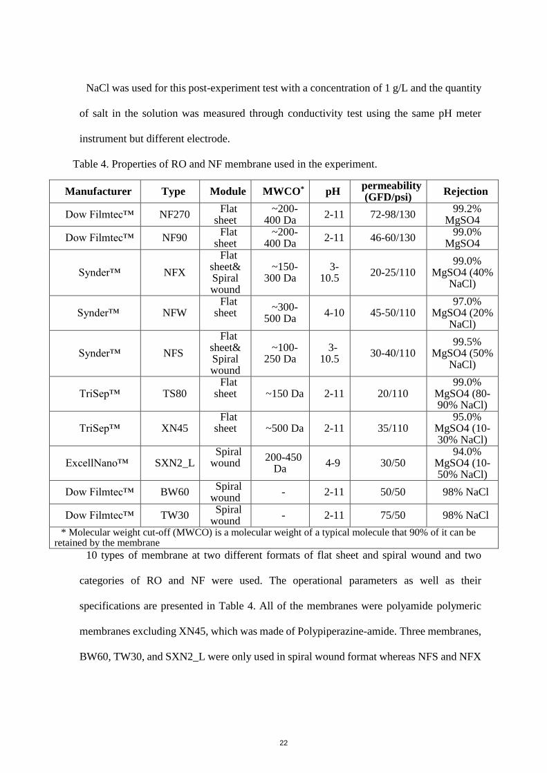
Table 4. Properties of RO and NF membrane used in the experiment.
Manufacturer Type Module MWCO* pH permeability (GFD/psi)
Rejection
Dow Filmtec™ NF270 Flat
sheet ~200-
400 Da 2-11 72-98/130
99.2% MgSO4
Dow Filmtec™ NF90 Flat
sheet ~200-
400 Da 2-11 46-60/130
99.0% MgSO4
Synder™ NFX
Flat sheet& Spiral wound
~150-300 Da
3-10.5
20-25/110 99.0%
MgSO4 (40% NaCl)
Synder™ NFW Flat
sheet ~300-
500 Da 4-10 45-50/110
97.0% MgSO4 (20%
NaCl)
Synder™ NFS
Flat sheet& Spiral wound
~100-250 Da
3-10.5
30-40/110 99.5%
MgSO4 (50% NaCl)
TriSep™ TS80 Flat
sheet ~150 Da 2-11 20/110 99.0%
MgSO4 (80-90% NaCl)
TriSep™ XN45 Flat
sheet ~500 Da 2-11 35/110 95.0%
MgSO4 (10-30% NaCl)
ExcellNano™ SXN2_L Spiral
wound 200-450
Da 4-9 30/50
94.0% MgSO4 (10-50% NaCl)
Dow Filmtec™ BW60 Spiral
wound - 2-11 50/50 98% NaCl
Dow Filmtec™ TW30 Spiral
wound - 2-11 75/50 98% NaCl
* Molecular weight cut-off (MWCO) is a molecular weight of a typical molecule that 90% of it can be retained by the membrane
10 types of membrane at two different formats of flat sheet and spiral wound and two
categories of RO and NF were used. The operational parameters as well as their
specifications are presented in Table 4. All of the membranes were polyamide polymeric
membranes excluding XN45, which was made of Polypiperazine-amide. Three membranes,
BW60, TW30, and SXN2_L were only used in spiral wound format whereas NFS and NFX
23
were available in both flat sheet and spiral wound formats. The reported pH in the table
represents for the operational pH range reported by the manufacturer of each membrane.
Results and Discussion
The results and discussion is divided into three parts, the first part focuses on the results
obtained from characterisation of wastewater, and the second part discusses the results
related to the activated carbon and membrane filtration treatment processes and the third
part is allocated on process modelling.
Figure 4. The frequency value of COD of 75 sample of raw wastewaters that were collected
from Aevitas over 10 months; the COD of 13% of the samples were below 600 while 77% of
the samples had a COD between 600 and 4000.
As already mentioned, the main problem of Aevitas (the major focus on this project) was
the COD values of higher than 600 in the effluent. To this ends, all collected samples were
measured for their COD and TOC, and pH. The results of the COD measurements are
presented in Fig. 4. This figure shows how many untreated samples in 75 samples had the
COD value more than 600. According to the Fig. 4, the vast majority of samples had the

24
COD values between 600 and 4000, which means the more effort should be performed in
this range of COD.
3.1. Identifications and occurrences of organic chemicals in industrial wastewater
After analyzing the wastewater provided from the Aevitas, their chemical composition was
identified using GC/MS. As mentioned, 150 industrial wastewater samples were
characterized before treatment (75 samples) and after treatment (75 samples) using activated
carbon. The results of GC/MS spectrum could identify 1250 chemicals from different
categories (e.g. organic acid, alcohols).
Table 5.The chemicals with high occurrences in Aevitas wastewater. These chemical are the
results of 150 samples, which 75 of them were before treatment and 75 were after treatment.
Chemicals Occurrences
RT
(min)
Mw
(g/mol)
Log
Kow
Ethylene glycol butyl ether 73 5.6 118 0.83
Benzyl alcohol 60 7.3 108 1.1
Dodecanedioic acid 55 19.7 230 3.2
Benzoic acid 53 9.1 122 1.87
Diethylene glycol butyl ether 53 9.9 162 0.56
2-Ethylhexanoic acid 51 6.6 144 2.64
Sebacic acid 50 17.5 202 1.5
Octanoic acid 46 8.2 144 3.05
Hexanoic acid 38 5.6 116 1.92
1,11-Undecanedioic acid 38 18.6 216 NA
Phenol 31 5.8 94 1.46
Triethylene glycol butyl ether 31 14.3 206 0.02
Dicyclohexylamine 31 11.4 181 4.37
Nonanoic acid 30 9.6 158 3.42
Phenoxyethanol 25 11 138 1.16
Hexadecanoic acid 23 18.5 256 7.17
Heptanoic acid 22 6.8 130 2.42
2-Phenylethanol 13 8.4 122 1.36
Isoeugenol 12 12.7 164 3.04
Ricinoleic acid 9 22.4 298 6.19

25
Table 5 shows the chemicals with high occurrences in Aevitas industrial wastewater.
According to the Table 5, chemicals with high occurrence in the industrial wastewater are
used widely in many industries such as solvent-based coatings, water-based printing inks,
pesticides synthesizing, and so on [33]. While the Mw of the all the identified chemicals are
more than 100 g/mole, phenol is the one which has Mw of 94. The major concern in this
table is Hexadecanoic acid due to the value of log Kow (the ratio of the concentration of a
chemical in n-octanol and water at equilibrium at a specified temperature) which is higher
than 4. The Kow of the most of the xenobiotic compounds is higher than 4 which means these
compounds are more likely to bio-accumulate in living organisms and compounds [34]. Fig.
5 are provided to indicate the variation in the spectrum where different wastewaters were
used to identify the chemicals in the medium. The spectrum of four wastewaters ED42,
ED52, ED65, and ED68 are shown in Fig. 5, while their COD were different as well. It
seems that there is no correlation between the number of sharp peaks and the value of COD;
however, there is a strong correlation between the intensity of the peaks and their COD. For
example, in wastewater ED42 (Fig.5A) and ED68 (Fig.5D) the amount of COD is about
5000 and higher than ED52 (Fig.5B) and ED65 (Fig. 5C) (where their COD is below 1000)
and so, their related sharp peaks in the spectrum are more intense than the peaks in ED52
and ED65.

26
1 2 3
45
6
7
8
9
10
11
12
13 14
15
16
1718
6 8 10 12 14 16 18 20 22 Time [min]0.0
0.5
1.0
1.5
2.0
2.5
7x10
Intens.
ED18-0049.D: TIC +
123
4
56
78 9101112
13
14151617
1819
2021 22
232425 26 27 28 29 30 3132 33 34
35
3637
38 39
4041
6 8 10 12 14 16 18 20 22 Time [min]0.0
0.2
0.4
0.6
0.8
1.0
7x10
Intens.
ED18-0061.D: TIC +
1 2 3
45
678 9 10 11 12 13 14 1516 17
6 8 10 12 14 16 18 20 22 Time [min]0
2
4
6
7x10
Intens.
ED18_0091.D: TIC +
1 Ethylene glycol butyl ether
2 2-Ethylhexanoic acid
3 Linalool
4 Benzyl alcohol
5 ?
6 ?
7 ?
8 ?
9 Octanoic acid
10 Benzoic acid
11 diethylene glycol, butyl ether
12 ?
13 Decanoic acid
14 Dodecanoic acid
15 ?
16 Sebacic acid
17 Hexadecanoic acid
18 1,11-Undecanedioic acid
1 ? 21 ?
2 ? 22 ?
3 ? 23 ?
4 Ethylene glycol butyl ether 24 Diethylene glycol, butyl ether
5 Hexanoic acid 25 ?
6 Phenol 26 ?
7 ? 27 ?
8 ? 28 ?
9 2-Ethylhexanoic acid 29 Triethylene glycol, butyl ether
10 Heptanoic acid 30 ?
11 ? 31 ?
12 ? 32 ?
13 Benzyl alcohol 33 Sebacic acid
14 ? 34 ?
15 ? 35 1,11-Undecanedioic acid
16 ? 36
17 ? 37 Dodecanedioic acid
18 Octanoic acid 38 ?
19 ? 39 ?
20 ? 40 ?
41 ?
1 Propylene glycol
2 ?
3 Linalool
4 2-Ethylhexanoic acid
5 ?
6 Nonanoic acid
7 Benzyl alcohol
8 ?
9 ?
10 ?
11 Benzoic acid
12 Phenoxyethanol
13 Benzenepropanoic acid
14 ?
15 1,11-Undecanedioic acid
16 ?
17 Internal Standard
A
B
C

27
Figure 5. GC/MS spectrum of four industrial samples received from Aevitas; A) ED42,
COD=4970 with 18 sharp peaks (67% known + 33% unknown); B) ED52, COD=720 with 41
sharp peaks (29% known + 71% unknown) C) ED65, COD=974 with 17 sharp peaks (59%
known + 41% unknown); D) ED68, COD=6172 with 9 sharp peaks (89% known + 11%
unknown). There is a positive correlation between the COD values and maximum intensity of
the peaks (for spectrum (D) is 4.5×10⁻⁷ while for spectrum (B) is below 0.1×10⁻⁷).
3.2. Adsorption of organic chemicals during Activated Carbon Process
The adsorption process were conducted through two formats. One in batch process and the
other one was in column test.
3.2.1. Batch Process Activated Carbon Adsorption
Fig. 6 shows the COD of the samples that have been used for characterisation (with ED
code) and then activated carbon was added into these wastewaters for COD removal of the
wastewater. After treatment, only 28% of the wastewater had a COD higher than 600 and
the rest of them could be discharged into the municipal wastewater treatment plant by
meeting the standard requirement (while this value already was about 87%). According to
the Fig. 6, despite applying the same ratio of activated carbon to TOC, the COD removal
was different from one sample to another. This means that the COD removal is highly
affected by chemical composition of the used wastewater.
1
2
3
4
5
6
7
89
6 8 10 12 14 16 18 20 22 Time [min]0
1
2
3
4
7x10
Intens.
July5_18.D: TIC +
1 Ethylene glycol butyl ether
2 2-(2-Methoxyethoxy)ethanol
3 2-Ethylhexanoic acid
4 Nonanoic acid
5 Benzoic acid
6 ?
7 Sebacic acid
8 1,11-Undecanedioic acid
9 Dodecanedioic acid
D

28
0 1000 2000 3000 4000 5000 6000 7000 8000 9000
ED1
ED29
ED30
ED31
ED32
ED33
ED34
ED35
ED36
ED37
ED38
ED39
ED40
ED41
ED42
ED43
ED44
ED45
ED46
ED47
ED48
ED49
ED50
ED51
ED52
ED53
ED54
ED55
ED56
ED57
ED58
ED59
ED60
ED61
ED62
ED63
ED64
ED65
ED66
ED67
ED68
ED69
ED70
ED71
ED72
ED73
ED74
COD (ppm)
Was
tew
ater
Sam
ple
sInitial COD End time COD

29
Figure 6. Treatment of the collected samples from Aevitas using activated carbon
adsorption; the empty redline and the full blue bars are the amount of COD at the time before
adding activated carbon and at the end of experiment, respectively. The applied amount of
applied activated carbon for each experiment depends on the amount of their TOC were kept
constant (1-gram activated carbon per 10 mg of TOC).
Fig. 7 A and B are provided to indicate how activated carbon can remove the vast majority
of the organic chemicals. According to Fig. 7 A and B, the red line corresponds to the
untreated wastewater and the blue line is the spectrum of the same sample after 24 h being
treated using activated carbon. Several sharp peaks have appeared in the spectrum before
treatment, whereas these peaks have been eliminated after treatment, which means that
activated carbon successfully adsorbed the chemicals. Although the COD of the both ED42
and ED68 were about 5000 and higher, their COD removal percentage were 64 and 30%,
respectively. In the both spectrum, it is difficult to observe the blue line, because of the low
concentration of the detectable chemicals by GC/MS.
The other important results from batch experimentation showed that 1 gram of activated
carbon adsorbs 7 mg of TOC or 25 mg of COD from industrial wastewater. These values
are average number and clearly depending on the composition of the wastewater, (the values
can be more or less).

30
Figure 7. The full GC/MS spectrum of two samples (ED42 (A) and ED68 (B)) before
treatment (redline) and after treatment (blue line) using activated carbon. Activated carbon
successfully adsorbed all the detectable chemicals by GC/MS from wastewater and thus the
COD values decreased.
3.2.2. Sequential Activated Carbon Adsorption
Sequential adsorption process using activated carbon was applied for wastewater treatment
to observe if the remained chemicals can be adsorbed on the surface of new activated carbon.
According to the Fig. 8, two different kind of industrial wastewaters BW7 (diluted) and
BW8 were used for treatment using activated carbon (Continental Carbon Group).
Experiments related to both first and second batches were carried out three times. The initial
COD for the wastewater BW7 (diluted) and BW8 were 2016 and 748, respectively, while
the original COD of the BW7 was 8400. The COD removal for BW8 in the first batch was
measured as 76% whereas in the second batch using the new activated carbon (unused) the
12 3
45
6
7
8
9
10
11
12
13 14
15
16
1718
6 8 10 12 14 16 18 20 22 Time [min]0.0
0.5
1.0
1.5
2.0
2.5
7x10
Intens.
ED18-0049.D: TIC + ED18-0049AT.D: TIC +
1
2
3
4
5
6
7
89
6 8 10 12 14 16 18 20 22 Time [min]0
1
2
3
4
7x10
Intens.
July5_18.D: TIC + JULY5_18AT.D: TIC +
1 Ethylene glycol butyl ether
2 2-(2-Methoxyethoxy)ethanol
3 2-Ethylhexanoic acid
4 Nonanoic acid
5 Benzoic acid
6 ?
7 Sebacic acid
8 1,11-Undecanedioic acid
9 Dodecanedioic acid
1 Ethylene glycol butyl ether
2 2-Ethylhexanoic acid
3 Linalool
4 Benzyl alcohol
5 ?
6 ?
7 ?
8 ?
9 Octanoic acid
10 Benzoic acid
11 diethylene glycol, butyl ether
12 ?
13 Decanoic acid
14 Dodecanoic acid
15 ?
16 Sebacic acid
17 Hexadecanoic acid
18 1,11-Undecanedioic acid
ED42; COD before treatment=4970ppm
COD after treatment=1760 ppm
ED68; COD before treatment=6172 ppm
COD after treatment=4332 ppm
A
B

31
removal percentage dropped by 40%. Although there was the same percentage drop of the
COD for BW7 was observed in the second batch, the COD removal at the first stage was
around 57%. This means that the organic chemicals in BW8 have more tendency to be
adsorbed on the surface of the activated carbon. The applied ratio of the amount of activated
carbon to the mass of TOC in the wastewater was kept constant at 100 mg AC/mg TOC.
Furthermore, the remained chemicals after the first batch were not able to be adsorbed on
the surface of the new activated carbon. These chemicals might be polar and have a very
low Mw (under 100 g/mole) as they have a very low affinity with activated carbon. In this
regards, a surrogate wastewater has been prepared and then activated carbon was used for
treatment of this wastewater. Methanol was the main source of COD in the surrogate
wastewater with value of 2000 (Similarly, the same amount of surrogate was applied).
Figure 8. Sequential adsorption of organic chemicals from BW7 (diluted) and BW8 on the
surface of activated carbon (continental carbon group); initial COD of BW7 (diluted) and
BW8 were 2016 and 748, respectively; initial activate carbon in BW7 and 8 were 5.33 and
1.8 gram, respectively. The COD removal at the second stage was significantly lower than
the first stage of adsorption.
0
10
20
30
40
50
60
70
80
90
First Batch Second Batch
CO
D r
emoval
%
Batches
BW7 BW8
32
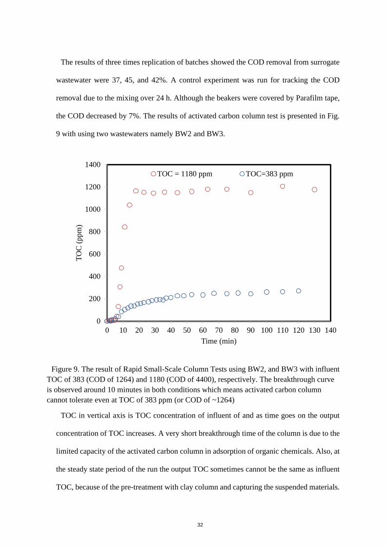
The results of three times replication of batches showed the COD removal from surrogate
wastewater were 37, 45, and 42%. A control experiment was run for tracking the COD
removal due to the mixing over 24 h. Although the beakers were covered by Parafilm tape,
the COD decreased by 7%. The results of activated carbon column test is presented in Fig.
9 with using two wastewaters namely BW2 and BW3.
Figure 9. The result of Rapid Small-Scale Column Tests using BW2, and BW3 with influent
TOC of 383 (COD of 1264) and 1180 (COD of 4400), respectively. The breakthrough curve
is observed around 10 minutes in both conditions which means activated carbon column
cannot tolerate even at TOC of 383 ppm (or COD of ~1264)
TOC in vertical axis is TOC concentration of influent of and as time goes on the output
concentration of TOC increases. A very short breakthrough time of the column is due to the
limited capacity of the activated carbon column in adsorption of organic chemicals. Also, at
the steady state period of the run the output TOC sometimes cannot be the same as influent
TOC, because of the pre-treatment with clay column and capturing the suspended materials.
0
200
400
600
800
1000
1200
1400
0 10 20 30 40 50 60 70 80 90 100 110 120 130 140
TO
C (
ppm
)
Time (min)
TOC = 1180 ppm TOC=383 ppm

33
The column itself was saturated between 10 and 20 min after running the experiment. Here,
the concentration of TOC is reported instead of the COD because the strong correlation was
found between COD and TOC with high coefficient of determination.
3.3. Pressure-driven membrane filtration for separation of organic chemicals from
wastewater
The main purpose of using membrane filtration was COD reduction, the same as the
activated carbon process. As mentioned, 12 wastewaters (named BW1, BW2, …, BW12)
with different chemical compositions were used for membrane filtration process. At the first
step of filtration, the results obtained from wastewater characterisation were analysed
statistically (in the out of the confidence interval of 95%) and the results confirmed that
BW9 and BW12 were two wastewaters with abnormal properties in comparison with the
other wastewater samples. According to the Fig. 10, one of the reasons that makes BW12
abnormal is related to the high amount of suspended solid in the wastewater, which for
BW12 is measured about 504 NTU before treatment and this value was 10 times higher than
normal wastewater. This picture compares between two wastewater samples, one normal
(BW11) and the other one, which is outlier (BW12). The high amount of suspended solid in
BW12 can be a source of COD and as this particles were not well dissolved in water and
the size of particles are large, thus, they can easily be removed by membrane filtration. In
this occasion, the COD of the influent is very high, while the rejection percentage is very
high as well, which means the composition of the wastewater is abnormal. Since in most
cases there were some portion of organic chemicals that could pass through the membrane,
the composition of the COD in permeate samples are significant.
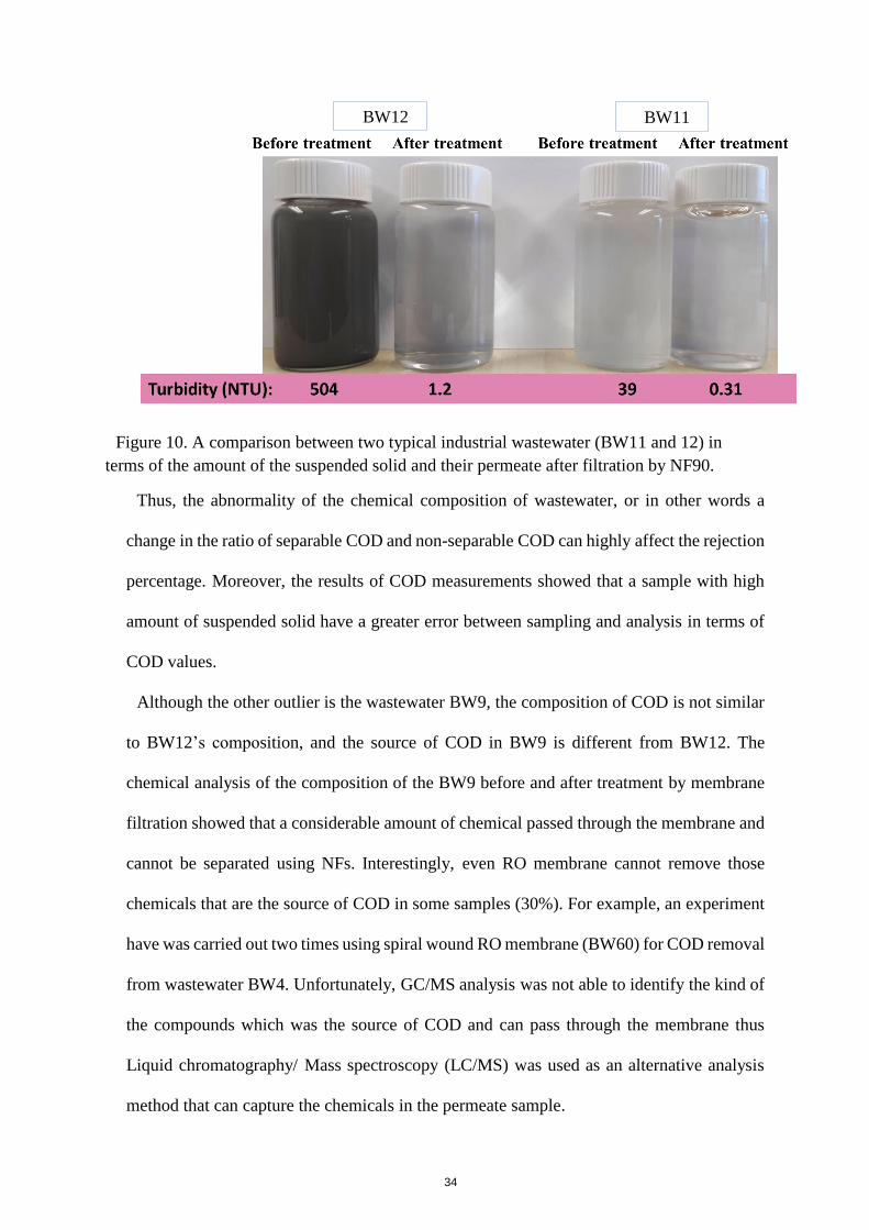
34
Figure 10. A comparison between two typical industrial wastewater (BW11 and 12) in
terms of the amount of the suspended solid and their permeate after filtration by NF90.
Thus, the abnormality of the chemical composition of wastewater, or in other words a
change in the ratio of separable COD and non-separable COD can highly affect the rejection
percentage. Moreover, the results of COD measurements showed that a sample with high
amount of suspended solid have a greater error between sampling and analysis in terms of
COD values.
Although the other outlier is the wastewater BW9, the composition of COD is not similar
to BW12’s composition, and the source of COD in BW9 is different from BW12. The
chemical analysis of the composition of the BW9 before and after treatment by membrane
filtration showed that a considerable amount of chemical passed through the membrane and
cannot be separated using NFs. Interestingly, even RO membrane cannot remove those
chemicals that are the source of COD in some samples (30%). For example, an experiment
have was carried out two times using spiral wound RO membrane (BW60) for COD removal
from wastewater BW4. Unfortunately, GC/MS analysis was not able to identify the kind of
the compounds which was the source of COD and can pass through the membrane thus
Liquid chromatography/ Mass spectroscopy (LC/MS) was used as an alternative analysis
method that can capture the chemicals in the permeate sample.
BW12 BW11

35
A t-statistic was performed on the two groups of RO and NF membranes that treating
random wastewater samples provided from Aevitas. The t-test indicated RO had a better
performance than NF in terms of COD removal. However, one of the main drawbacks of
the RO is related to the low flux and the short length time that takes for the membrane,
which causes rapid fouling of the membrane. To overcome this problem NF membrane can
be used to obtain a higher flux as well as keeping the acceptable COD removal percentage.
However, the experimental results showed that different NF membranes, which have been
manufactured by same company with the same MWCO had different permeate flux. For
example, the NF270 and NF90 are manufactured by Dow (Filmtech) and according to the
company the MWCO of these two membranes falls within the same range of 200-400Da.
While according to a study, the values of NF270 and NF90 have been estimated as 340Da
and 180Da, respectively [35] (which there is close consistency between that study and the
obtained results in our experiments)
3.3.1. COD removal from wastewater using different membranes
Since the wastewater BW9 has shown an abnormal characteristic, experiments were
designed to observe the performances between different NF membranes in terms of COD
removal. The original COD and TOC of this wastewater was about 9400 and 4220,
respectively. As mentioned in Fig. 4, the COD of the most of the samples falls within the
1000 and 4000. Thus, to keep the concentration of COD at the same range the wastewater
was diluted into two levels of COD ~2000 and ~4000. To design an effective experiment
two levels of COD including 2000 and 4000 plus using 6 types of different flat sheet NF
membranes including NFX (Synder), NF90 (Dow Filmtec), TS80 (TriSep™), NFW
(Synder), NF270 (Dow Filmtec), and XN45 (TriSep™). The number of experiments with
replication were 24 and randomized runs. Although there was a difference between

36
hypothetical influent COD and the real diluted COD of industrial wastewater to run the
experiments, in most of cases, the deviation was less than 10%. Despite working in two
levels of COD in the experiments, the statistical analysis evidently showed that the
concentration of COD is not a key factor in COD removal, whereas the type of membrane
significantly affects the COD removal (see Table 6).
Table 6. ANOVA table for the experiments using BW9.
Source DF Adj SS Adj MS F-Value P-Value
Regression 11 1980 180 13.88 0.000
COD 1 64.68 64.68 4.99 0.045
NF-Membrane types 5 425.25 85.05 6.56 0.004
COD*NF-Membrane types 5 149 29.92 2.31 0.109
Error 12 155.59 12.97
Total 23 2135
R2 (adj)=86%
Based on the ANOVA table there is no interaction between the influent concentrations of
COD and the type of membrane. For example, if a membrane shows a lower performance
in COD removal (for a specific wastewater), the rest of the membranes may show the same
performance but with a different ratio of reduction of COD removal. To confirm the results,
Fig. 11 indicates that the COD removal variation for both concentrations of COD, 2000 and
4000 ppm (BW9) is almost similar where a particular membrane was used. The other main
point that can be learned from Fig. 11 is the great performance of the NF90 in COD removal
of BW9 and the poor COD removal of NFW and NF270. The red dashed line in Fig. 11
marks for the maximum allowable COD level for discharging effluent into the municipal
sewer where NF90 can reduce the COD to around 600.
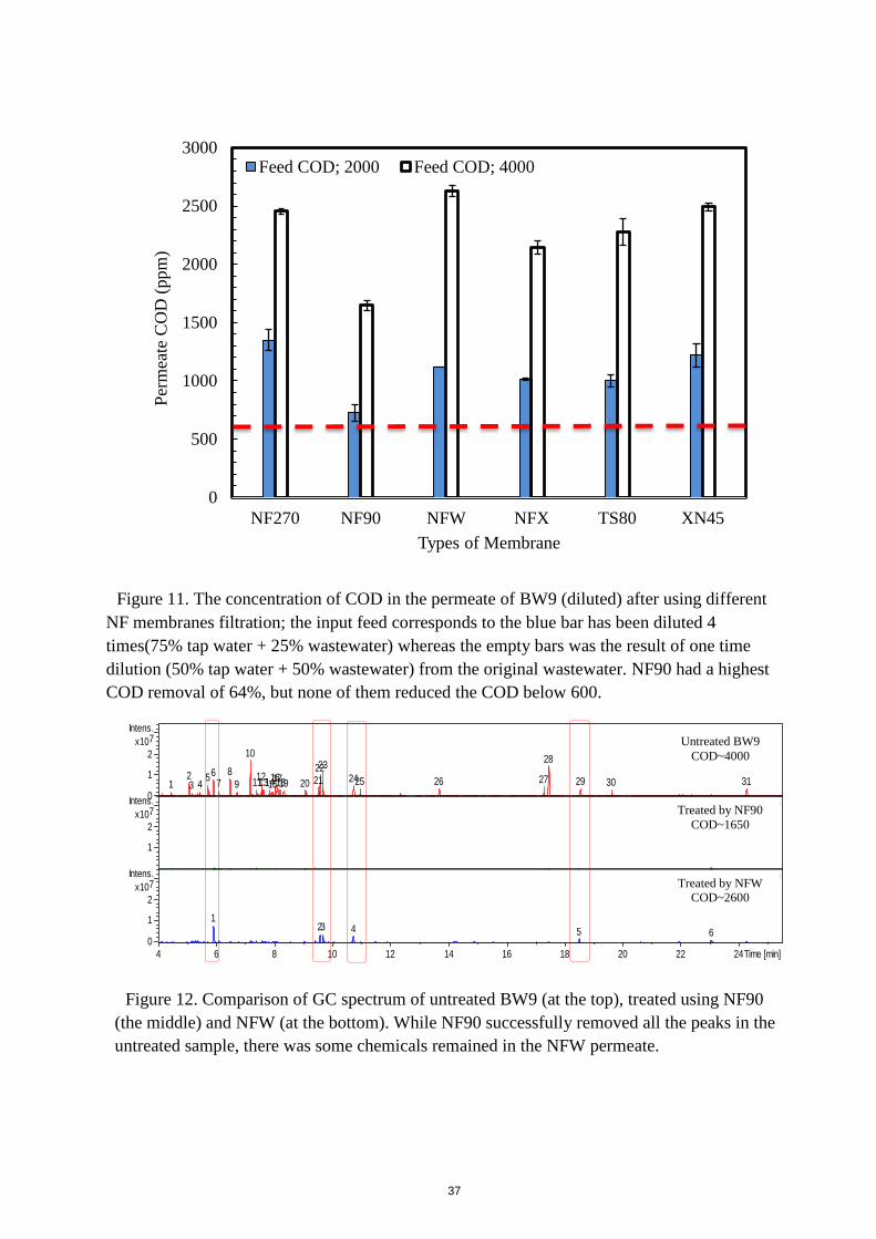
37
Figure 11. The concentration of COD in the permeate of BW9 (diluted) after using different
NF membranes filtration; the input feed corresponds to the blue bar has been diluted 4
times(75% tap water + 25% wastewater) whereas the empty bars was the result of one time
dilution (50% tap water + 50% wastewater) from the original wastewater. NF90 had a highest
COD removal of 64%, but none of them reduced the COD below 600.
0
500
1000
1500
2000
2500
3000
NF270 NF90 NFW NFX TS80 XN45
Per
mea
te C
OD
(ppm
)
Types of Membrane
Feed COD; 2000 Feed COD; 4000
123 4
567
8
9
10
1112131415
16171819 20 21
2223
2425 26 27
28
29 30 31
BW9Original.D
NF90_4000_BEST.D
123 4 5 6
NFW_4000_WORST.D
0
1
2
7x10
Intens.
1
2
7x10
Intens.
0
1
2
7x10
Intens.
4 6 8 10 12 14 16 18 20 22 24Time [min]
The COD of untreated WW~4000
The COD of NF90 permeate = 1650
The COD of NFW permeate = 2600
Untreated BW9
COD~4000
Treated by NF90
COD~1650
NF90
Treated by NFW
COD~2600
Figure 12. Comparison of GC spectrum of untreated BW9 (at the top), treated using NF90
(the middle) and NFW (at the bottom). While NF90 successfully removed all the peaks in the
untreated sample, there was some chemicals remained in the NFW permeate.

38
In order to observe the differences between the performance of the membranes in terms of
chemicals removal, a GC/MS spectrum of the untreated wastewater (BW9) and the treated
wastewater using NF90 (as the best candidate of COD removal) and NFW (as the poor
membrane) were shown in Fig. 12. According to the spectrum, there are at least 31
chemicals in the untreated wastewater that have significant peaks appeared by GC/MS
analysis, whereas all of these chemicals have been eliminated by NF90 (the middle
spectrum) so that no peaks appear in the spectrum. While there are still some peaks which
shows the presence of some of the organic chemicals in the permeate sample of the NFW
membrane. The removal efficiency percentage (shown in Table 7) was calculated by
normalizing the area under the peaks (by dividing them by the area of internal standard).
Accordingly, the removal of Butanoic acid using NFW is almost ignorable whereas NF90
can separate it by 91%. Although GC/MS cannot identify all the peaks appeared in the
spectrum and some of them are introduced as unknown, their removal percentage can be
calculated.
Table 7. Removal percentage of chemicals from BW9 using NF90 and NFW in according to
Fig. 12.
The other interesting observation related to Fig. 12 is the amount of the COD in the
permeate samples (1650 ppm) where NF90 was used, while there are no peaks in the
spectrum marking for chemicals. Thus, there still are some organic chemicals in the
permeate samples (as it is confirmed by TOC and COD analysis) that cannot be detected by
GC/MS. In order to identify such chemicals, complementary sample preparations or using
Peak
number
RT
[min] Compounds
Removal% using
NF90 separation
Removal% using
NFW separation
6 5.89 Butanoic acid 91 0
22 9.55 Unknown 98 70
23 9.66 Unknown 97 69
24 10.7 Unknown 97 51
29 18.52 1,11-Undecanedioic acid 95 55

39
other analytical instruments (Liquid chromatography) might requires for further insight.
Although GC/MS is a high performance characterisation technique, it can only capture those
chemicals that are volatile or can be separated at a higher temperature without any
deformation of the molecular structure [36].
3.3.2. Membrane filtration COD removal versus flux
As already indicated in Fig. 11, three NF flat sheet membranes (NFX, TS80, and NF90)
showed a better performances in terms of COD removal and thus, these three membranes
were chosen for conducting further experiments. Three different wastewaters named BW11,
BW12, and BW12 (at 3 different levels of COD, 1100, 1700, and 4200) were used to observe
the COD removal percentage.
Figure 13. COD removal of three different wastewaters three wastewater BW10 (COD:
1100), BW11 (COD: 1100), and BW12 (diluted COD: 1700), BW12 (COD: 4200) using
NFX, TS80, and NF90 flat sheet NF membranes. NF90 had a better performnce than others
did.
0 20 40 60 80 100 120
BW 10 - 1100 mg/L
BW 11 - 1100 mg/L
BW 12- 1700 mg/L
BW 12 - 4200 mg/L
COD removal%
BW
s
COD removal %NFX TS80 NF90

40
The original COD of the BW12 was about 4200, and thus has been diluted by tap water to
get the COD to the practical COD level (~1700). Based on Fig. 13, the overall COD removal
of NF90 was still the highest while the difference between the performances of NF90, TS80,
and NFX was not significant statistically. All three membranes can successfully remove
almost more than 80 % of COD with no significant affecting from the type of wastewaters.
If a membrane is intended to be used for industrial wastewater treatment the other important
parameter would be the permeate flux of membrane. Fig. 14 is provided to make a comparison
between the permeate fluxes where different industrial wastewaters (BW10 (COD: 1100),
BW11 (COD: 1100), and BW12 (diluted COD: 1700), BW12 (COD: 4200)) were used.
Although the COD removal of NF90 and TS80 was relatively high, their permeate flux was not
as high as that of NFX.
Therefore, there exists the trade-off between COD rejection and the permeate flux in
industrial application. Due to the high amount of suspended solid in BW12 the permeate
flux was affected by deposition of colloidal and solid particles on the surface of the
membrane and blocking the pores of the NFs. In this occasion, to overcome the problem a
microfiltration is needed to be installed before the NF so that the suspended solids and large
colloidal particles can be separated from the wastewater earlier. This change can results in
a higher permeate flux although it will take longer to complete the treatment. Designing a
clarifier or a settling tank are the other options for solving this he mentioned issue. Without
the pre-treatment steps, the membrane will be fouled and with a drop in flux.

41
Figure 14. Flux of three different flat sheet NF membranes; NFX, TS80, and NF90, which
were used for treating three wastewater BW10 (COD: 1100), BW11 (COD: 1100), and
BW12 (diluted COD: 1700), BW12 (COD: 4200), NFX had a better flux than others did.
3.4. Sequential membrane filtration followed by activated carbon process
An attempt was made to observe the effectiveness of integrated wastewater treatment using
membrane filtration followed by activated carbon. Activated carbon was used for further
treatment of permeate sample of both RO and NF. The experimental results showed that
activated carbon can adsorb about ~20% of the COD from the RO’s (BW60 and TW30)
permeate (BW7). This means the organic chemicals that can pass through the RO have a
low tendency for being adsorbed on the activated carbon. The original COD of the BW7
was about ~8400 and so was diluted for being prepared for the experiment. The feed COD
into the RO (BW60 and TW30) was ~1000 and the output permeate COD was measured
~365, which indicates a 63% of COD removal only by using the membrane. Treating the
permeate sample (from RO) with the activated carbon could further reduce the COD by
0 0.2 0.4 0.6 0.8
BW 10 - 1100 mg/L
BW 11 - 1100 mg/L
BW 12- 1700 mg/L
BW 12 - 4200 mg/L
Flux(L/m2/min)
BW
sFlatsheet membrane flux
NFX TS80 NF90
42
20%. Applying NF membrane also showed similar results as RO did, for example, both flat
sheet and spiral wound NFX reduced the COD by 60% (BW7) whereas the activated carbon
could only adsorb 16% of the COD from the permeate samples. According to Fig. 15, as
long as membrane has a good performances in COD removal (i.e. 60%) (i.e. XN45), the
activated carbon adsorption process only remove 20% of the remaining COD, while the
permeate from a poor membrane rejection (i.e. XN45) can be treated efficiently by activated
carbon. It seems the chemicals that pass through XN45 have a great tendency for being
adsorbed on the surface of the activated carbon. For example, the COD removal from XN45
permeate was about 28% in the post treatment step using activated carbon. The poor
separation efficiency of the XN45 might be attributed to the high MWCO of this membrane
which is ~500Da (similar to NFW) and the probably due to the used polymeric material
(polypiperazine). A GC/MS spectrum is provided to monitor the performances of the
integrated membrane – activated carbon process. This spectrum strongly confirmed the bulk
measurement results of COD in feed, permeate, and after treating by the activated carbon.
Since many of the peaks (each peak is candidate for a chemical) in the feed wastewater were
eliminated after the treatment by membrane filtration, while in the next stage, activated
carbon was not significantly influence the magnitude of the peaks . As indicated in Fig. 16,
NFX spiral wound membrane separates two chemicals (Nonanoic acid and 2-Ethylhexanoic
acid) which are the main source of COD in the BW7. Since the COD value of 1315 in the
feed reduced to 511 in the permeate flow, it can be inferred that the cumulative COD of
these eliminated peaks were about ~805.

43
Figure 15. Sequential membrane (RO and NFs)-activated carbon treatment of wastewater
(BW7) containing organic chemicals using. BW7 with original COD of 8400 was diluted for
being used as an actual feed with a normal COD. Membrane filtration as first step had a great
contribution in COD removal.
Figure 16. GC/MS spectrum of diluted BW7 when being treated by sequential membrane
(NFX spiral wound)-activated carbon process. The COD of the feed, permeate, and treated
permeate by activated carbon were, 1315, 511, and 475, respectively. Membrane filtration
reduced the peaks considerably, while, the influence of activate carbon was not significant.
0
500
1000
1500
2000
2500
BW60 TW30 NFX
Spiral
wound
NFX
Flatsheet
NFW XN45 TS80
CO
D
Membrane types
Feed COD Permeate COD Treated by AC

44
3.5. Process modelling
An integrated PCA-ANN modeling was used to predict the quality of the wastewater (with
code EDxx) before and after treatment using activated carbon process. The source of the
data for develop the model was from analyzing the collected industrial wastewater treatment
plant during 10 months. After receiving the wastewater from the plant several parameters
associated with the wastewater were measured using different tests. All the variables that
are reported in this study called;
Case (as categorical factor which was 2 forms of wastewater quality before and
after treatment),
Amount of applied activated carbon (gram),
TOC (mg/L),
Capacity of adsorption,
COD (mg/L),
pH,
Number of sharp peaks (that has been appeared in the GC/MS spectrum),
RT 4-6 (number of peaks that have been shown after retention time of 4 till 6 min),
RT 6-8, RT 8-10, RT 10-12, RT 12-14, RT 14-16, RT 16-18, RT 18-20, and RT
20-24.
Only GC/MS analysis was the source of 9 variables. The retention time (RT) of the
spectrum resulted of GC/MS is from 4 min till 24 min and the number of sharp peaks, which
have been appeared every 2 min were considered one variable. The retention time from 4 to
20 min would be 8 variables plus two variables; one is the number of intense peaks after 20
min and the other one is the number of total peaks appeared in the spectrum. The other
parameters were the capacity and the amount of the applied activated carbon, the order of
45
the intensity of the peaks, and ultimately a categorical factor before and after treatment.
Therefore, sum of the all variables was 16.
3.5.1. Principal Component Analysis
PCA was the first model that has been built to analysis the quality of the industrial
wastewater during treatment process using activated carbon. The software named Aspen
ProMv was used to implement the model. PCA, as a method from big data, was used to
express the trend and correlation among the variables and observations (the observation here
means the characteristic of each sample before and after treatment using activated carbon)
due to the size of the data obtained in this work. PCA is a suitable technique for compacting
many data into something that comprises for the significant original data and the dataset
with many variables will be flattened in to 2 or 3 dimensions so that we can observe the
correlation among them [37]. The first principal component (PC1) is the line that can pass
through all the data and can explain the most variance. The PC2 with the similar procedure
is going to explain the most remaining variance of variables. As the number of component
is added in to the model the goodness of a fit (R2) increases where R2 is between 0 and 1
(R2 = 1 means best fit). The R2 it-self is the amount of variability at the training stage and
there is a similar value called Q2 which is an indicator of how much variation is related to
the test dataset. R2 and Q2 will be improved by adding components [38]. The outlier data
are determined based on the three statistic named T2 Hoteling (distance of every point from
center, taking (co)variance into account) and Squared prediction error (SPE (Distance off
the model plane). These two extensions are more effective statistic in big data analysis. The
Hoteling’s T2 value is a useful measure for monitoring the overall performance of the key
factors of a system. The advantages of T2 Hoteling is its flexibility, being easy to use,
presenting small changes in performances, and suggesting adequate marks to elucidate the

46
process. It is very similar to t-statistic, distance between the experimental data mean and
their related population mean. However, using the T2 Hoteling alone does not show all the
variances, a small amount of variance that has not been considered in the model and the
residuals, usually known as SPE. Thus, SPE and T2 Hoteling are complementary for
representing the residual [39]. Score plot is a helpful illustration that can be shown in PCA
and each observation in the plot is a representative of one score. The score plot containing
score values for each observation is a distance from the origin along the loading vector of
the first component [40]. Loading vector in the loading plot defines direction and the loading
itself is the correlation between components and the original variables. This helps us to
interpret the effectiveness of the factors and the relationship between variable and group
them in different categories based on their weights [41]. Moreover, along with this plot,
contribution plot can help observing which variable is effective which provides more insight
for making a decision to remove or keep the variables for the next step [41, 42]. Overall,
150 observations with 16 variables were used to build the PCA model.
3.5.2. Variation in Sampling, and outliers
Two analyses, SPE and T2 Hoteling have been used for showing the variation and the
samples with the unusual characteristics. Fig. 17 presents the SPE statistic that was obtained
from analysing the experimental data. This analysis showed that three wastewater samples
(observations) were out of the normal range (0.99 confidence interval) and for further
analysis, these three points were ignored. The abnormality of the observation have several
reasons, for example for this case, the value of COD and TOC was significantly lower than
expected level, and thus the analysis introduced these points as outliers.

47
Figure 17. Squared Prediction Error to show and eliminate the wastewater (with code
EDxx) that indicates abnormal properties; according to SPE, three data were ignored as they
were outliers.
The other analysis is T2 Hoteling the theoretical function of this method has already been
introduced and Fig. 18 is a demonstration of this analysis. According to the T2 Hoteling,
seven observations were in outside of the limit and have been eliminated from the model,
and then a new analysis was carried out. The physical interpretation from the abnormality
is attributed to the pH with out of normal range. Similar to the SPE the horizontal axis is the
observations or the characteristic of wastewater samples and the vertical axis shows the
remained residual in the model.
0
1
2
3
4
5
6
7
8
0 20 40 60 80 100 120 140
SP
E
Observations Number
Squared Prediction Error 0.95 0.99

48
Figure 18. T2 Hoteling statistic for outliers to show and eliminate the wastewater (with code
EDxx) that indicates abnormal properties; according to HT2, three data were ignored as they
were outliers.
3.5.3. Most Significant Process’s Parameters and Chemicals in Wastewater before and
after treatment using activated carbon
Table 8 indicates after applying 4 components, the improvement of both Q2 and R2 were
less than 10%, as a result, there was no point in using more components to build the model.
As the number of components increase the amount of the residual decreases and the model
would be more reliable. Since the numerical values of Q2 and R2 are very close, and the data
in training stage was randomized, the built model works independently of the particular data
that has been applied for training the PCA model.
0
5
10
15
20
25
0 10 20 30 40 50 60 70 80 90 100 110 120 130 140
HT
2
Observations Number
Hotelings T2 0.95 0.99

49
Table 8. The R2 and Q2 of the PCA modelling when more seven components were used; as
the number of components increases the model will be more accurate.
Training Num. R2 Cumulative Q
2 Cumulative
[1] 1 0.407401 0.391605
[2] 2 0.605222 0.586056
[3] 3 0.684606 0.641412
[4] 4 0.760122 0.732477
[5] 5 0.814914 0.789819
[6] 6 0.855303 0.819226
[7] 7 0.8932 0.868999
T Score plot of the model is shown in Fig. 19, and the samples before treatment were
mostly distributed at the right hand side of the plot whereas after treatment all the data shift
out to the left hand side of the plot. This graph shows if there is a sample of wastewater
which has not been well-treated by activated carbon and there is still no changes in the
characteristic of wastewater (no chemical adsorption). There might be some chemicals in
the wastewater that do not tend to be adsorbed on the activated carbon. According to this
plot, two observations are out of 0.95 confidence interval which belongs to the samples
before treatment with the highest values of COD and TOC. The samples after treatment are
more convergent than those before treatment. This means that the capacity of the applied
activated carbon was proper and thus the quality of the output samples was similar.
However, some of the samples after treatment were gathered at the top part of the T score
plot which implies that these industrial wastewater samples might belong to an specific
facility so that after treatment the quality of them were similar to each other but different
from the rest of the data.

50
Figure 19. T Score plot for PCA model. Untreated sample were placed in the right hand side
and after treatment by activated carbon they shifted into left hand side; this helps to see if a
conducted experiment was abnormal or the characteristic of sample before/after treatment
was abnormal.

51
Figure 20. Loading plot: the relationship between all the variables used to build PCA model
and shows which variable had the most similar influence in building the model.
Loading plot is one of the most useful plots from PCA model, which shows the group of
variables that have a similar influence on the quality of wastewater. Accordingly, in Fig. 20,
the retention time of the spectrum from 6 to 20 had almost the same effect on the quality of
the industrial wastewater whereas pH, retention time between 4-6 min, and the retention
time after 20 min are similar. As expected the adsorption process parameters including the
initial value of COD and TOC as well as the amount of activated carbon play a similar role.
AC(gr)
TOC(mg/L)
Capacity
COD(mg/L)
pH
Number of sharp peaks
RT4-6
RT-6-8
RT-8-10
RT-10-12
RT-12-14
RT-14-16 RT-16-18
RT-18-20
RT-20-24
-0.5
-0.4
-0.3
-0.2
-0.1
0
0.1
0.2
0.3
0.4
0.5
-0.5 0 0.5P[2
]
P[1]
52
Figure 21. Contribution plot of the PCA model based on the applied variables. This shows
the magnitude of the variation of each variable. The variation in RT-6-8 was the highest,
which means using activated carbon can remove all the peaks appeared between 6 and 8 min
in untreated sample.
Moreover, it is possible to observe the relative importance of each variable over the
contribution plot. The variables with the lowest contribution can be excluded from the
measurement item without any significant changes in the robustness of the built model.
Based on Fig. 21, most of the chemicals that are adsorbed on the surface of the activated
carbon have appeared in the retention time of 6-8 min and 16-18 min. While the number of
sharp peaks which are the index of the majority of the chemicals have undergone a
significant change. This means activated carbon is able to adsorb the vast majority of
chemicals in the industrial wastewater.
-0.8 -0.7 -0.6 -0.5 -0.4 -0.3 -0.2 -0.1 0 0.1
RT-6-8
Capacity
RT-16-18
Number of sharp peaks
RT-14-16
RT-12-14
AC(gr)
RT-8-10
RT-10-12
TOC(mg/L)
RT-18-20
COD(mg/L)
pH
RT4-6
RT-20-24
Weights
Var
iab
les
Contributions Plot
53
3.5.4. Artificial Neural Network
After preprocessing the data using PCA, and determining the significant variables (based
on Fig. 21), an effort was made to build a nonlinear model to predict the quality of the
effluent after being treated by activated carbon. The PCA model indicated that some of the
variables that have a minor contributions to the quality of water have been excluded for
developing the ANN model due to the improving the prediction process. Totally 649 data
over 11 variables (TOC, COD, Number of sharp peaks, RT 6-8, RT 8-10, RT 10-12, RT 12-
14, RT 14-16, RT 16-18, RT 18-20, AC (for input)/Capacity (for output)) were considered
as input and the same number of variables as the output. To determine the optimum number
of neuron in the hidden layer, different number of neurons, from 3 to 20, in the hidden layer
were evaluated, and then each topology was repeated 10 times. The topology with a
minimum value of mean square error and high correlation coefficient was selected. The trial
and error running the ANN showed that 2000 for the number of epoch would be enough for
these datasets (obtained from measuring the properties of wastewater before and after
treatment using activated carbon) and thus, the iterations for training was set on this number.
As shown in Fig. 22, after about 1600 epoch the MSE reached to a steady state. The data
randomly were introduced into the net and a function named Scaled Conjugate Gradient
(trainscg) was employed for the training stage. The best training process for this case was
Multi-Layer Feed Forward (MLF) according to the obtained results from trial and error
strategy. After conducting computational processes, the bias and weights were obtained to
define how much the input variable influence on outputs. The architecture of the built model
is shown in Fig. 23.

54
Figure 22. The calculated MSE for Train, Validation, and Test stages of the dataset
(obtained from measuring the properties of wastewater before and after treatment using
activated carbon).

55
Figure 23. Architecture of the built ANN model; 11 variables were considered as input of
649 data and the same number of variables were predicted based on the input; hidden layer is
non-linear and the output layer is linear.
3.5.5. Process performance prediction by definition of water quality using ANN
The built model was tested, then the best net in terms of the lowest MSE (~10-4) and the
highest coefficient of determination (0.67) were selected (Fig. 24) for further prediction.
According to Fig. 24, the model can explain the performance prediction of 68% of all the
data. The coefficient of determination of the three stages, training, validation and testing
was very close to each other, which means the built model is reliable. The number of the
neuron in the hidden layer found to be 13 that can predict the values for the outputs
optimally. The obtained weight and bias for the best net that will be used for further
prediction process using ANN. The main role of weights is to indicate the influence of the
input variables on the outputs. If the weights were near zero for a variable, then changing
the input does not change the output significantly and also positive weights mean decreasing
the input will increase the output.

56
Figure 24. Performances of the ANN in prediction quality of industrial wastewater treated
by activated carbon; the obtained MSE for building the model was ~10-4 and the R2 was 0.68.
It means this model can predict the quality of 68% of wastewater with confidence interval of
0.95.

57
Conclusions
The conclusions of this project are categorized in three different parts as the whole process
has been conducted in three stages including, characterisation, activated carbon, and
membrane filtration processes. At the first stage, industrial wastewater was collected from
Aevitas plant (before being drained into municipal wastewater treatment plant and after
partially oxidation-aeration stage) have been characterised using both bulk measurements
(COD, TOC, and pH) and species-based identification. The second stage is using activated
carbon for adsorbing the chemicals species in the wastewater to reduce the COD.
Furthermore, membrane filtration was considered and studied as an alternative treatment
process instead of activated carbon for the industrial wastewater treatment. The outcomes
are summarized below:
1) Conclusion from the first stage:
The chemical composition and the COD of the wastewaters, which were collected
from the Aevitas plant, are varying at different times of sampling as they receive
mixture of wastewater from different industries.
Characterisation of industrial wastewater using GC/MS is an effective way to
identify the chemicals that are source of COD; however, it does not show all the
organic chemicals. The results from GC/MS are helpful in designing an effective
process for wastewater treatment.
The results of bulk measurements have shown the COD of that most of the samples
that have been taken from the plant falls between 1000 and 4000. Therefore, the
population of the interested COD range is defined and an effective process is
needed to overcome the problem.

58
About 1250 chemicals were identified while the occurrence of some organic
chemicals were between 22 and 73. Most of these chemicals were from alcohol
and organic acid groups. The pH of these samples were between 5 and 8, which
does not require particular adjustment for being discharged to environment.
COD removal of a wastewater with COD of higher than 5000 and low amount of
TSS/turbidity is very difficult, especially by activated carbon and membrane
filtration. These kinds of wastewater usually contain very low Mw organic
chemicals that are likely polar. Interestingly, the chemicals, which were not
separated by activated carbon or membrane filtration, do not show significant
peaks in the GC/MS spectrum while TOC indicates a value for presenting organic
carbon in the wastewater.
The chemical composition of wastewaters BW4, BW7, BW9, and BW13 was quite
different. While the COD of all four samples were higher than 5000, the amount
of TSS in BW13 was ~10 times higher than the rest of the wastewaters.
2) Activated carbon process
The average amount of COD and TOC that can be adsorbed by 1 gram of activated
carbon are 25 and 7 mg, respectively.
The average COD removal from industrial wastewater using activated carbon is
about 67% with standard deviation of 18.6. On average 33% of COD in the Aevitas
industrial wastewaters cannot be adsorbed by activated carbon due to the several
factors which are related to the chemical properties such as polarity, size and the
molecular shape of chemicals, and hydrophobicity.
The adsorption of chemicals from industrial wastewater samples using activated
carbon can be modelled by multivariate big data (PCA) integrated by ANN so that

59
the quality of water before and after treatment can be predicted with an acceptable
reliability.
3) Membrane Filtration
Depending on the chemical composition of the wastewater, the COD removal in
the membrane filtration process can vary from 30 to 90%. For a typical wastewater
with high amounts of suspended solids (BW13) a pre-filtration using
microfiltration can be helpful from two aspects, one is membrane fouling during
longer time span and the other is effectiveness in COD removal.
BW4 and BW9 were two types of wastewaters that their COD were not decrease
under 600 using every types of NF and RO, however, NF90 can reduce the COD
of diluted BW9 (~2000) to under 1000.
The experimental results did not show any interactions between the types of
wastewater and used membranes for filtration.
Among the NF membranes, the COD removal of NF90, NFX, NFS, and TS80 was
higher than the other membranes. Moreover, in terms of permeate flux, the NFS
and NFX had a higher membrane permeate flux compared to the other membranes.
Therefore, NFX and NFS are two proper candidates for wastewater filtration with
a high rejection percentage and a high permeate flux.
Although the efficiency of integrated membrane-activated carbon process totally
was higher than either of the processes alone, the vast majority of COD removal
from the wastewater happened at the first stage (~80%).

60
Recommendations for future works
In order to better fractionate the chemical species related to COD, a parallel
analysis of GC/MS along with LC/MS/MS can be used for the identification of the
chemicals especially the ones that neither can be adsorbed on the surface of the
activated carbon nor separated by membrane filtration. To this end, an accurate
quantitative analysis of the concentration of the species is required. Then, a
comparison is needed to be made between the measured COD, TOC, and the
contribution of sum of the chemicals that have been identified by GC/MS and
LC/MS/MS.
In this work, a number of polymeric membranes have been used. Application of
polymeric membranes for industrial wastewater treatment suffer from several
drawbacks, especially if the TSS content of wastewater is high. Two major problems
are membrane fouling and membrane compatibility with different solvents (i.e.
methanol or ethanol) which can result in poor membrane filtration performance due to
swelling of the membrane. The best alternative for the challenges is using ceramic
membranes for filtration of wastewater containing variety of many different chemicals.
Although ceramic membranes have higher packing densities and are heavier than
polymeric membranes, they are more stable against the harsh operating conditions
such as extreme pH, and chemicals. Moreover, the life span of ceramic membranes are
longer than polymeric membranes [43].
Since most of the chemicals that have a low tendency of adsorption on the surface
of activated carbon are very small and polar, using other degradation-based
treatment methods, (e.g. Electrochemical Oxidation) may be appropriate for
61
further COD reduction after aeration process. This would be extraordinary
important as the Aevitas plant is using batch process, the same process, which is
common in electro-oxidation, however, the following process must be in optimum
working conditions. The introduced method carries several advantages; including
maintaining high effectiveness at even lower temperatures with production of less
amount of by-products. Two path of direct and indirect oxidation are common in
this process which results in a considerable reduction of COD [44].
One of the main problems associated with the Aevitas effluent is the high level of
toxicity of the chemicals in the effluent. Although the concentration of the
hazardous materials might be trace, it can have a negative effect on the
performance of the municipal wastewater treatment as microorganisms run it.
Therefore, an effective process in one system that can meet two requirements of
high COD reduction and toxic chemicals removal could be a proper remedy for the
challenge aroused. This system can be a combination of ozone process with
activated carbon in one system. The function of activated carbon is adsorption of
high toxic substances in the system and the role of ozonation process is
simultaneous volatilization of VOCs and oxidation of recalcitrant chemicals for
COD reduction.
62
References
[1] Ranade VV, Bhandari VM. Industrial Wastewater Treatment, Recycling and Reuse.
Elsevier Science; 2014.
[2] Cheremisinoff NP, Knovel. Handbook of Water and Wastewater Treatment Technologies.
Elsevier Science; 2002.
[3] The Treatment of Industrial Wastewater in Canada 2019
http://www.thomasnutrientsolutions.com/industrial-wastewater-canada/.
[4] Tebbutt THY. Principles of Water Quality Control. Elsevier Science; 1997.
[5] Jorgensen SE. Industrial Waste Water Management. Elsevier Science; 1979.
[6] Cristian O. Characteristics of the untreated wastewater produced by food industry. Analele
Universităţii din Oradea, Fascicula: Protecţia Mediului 2010; 15:709-714.
[7] Guerrero L, Omil F, Mendez R, Lema J. Anaerobic hydrolysis and acidogenesis of
wastewaters from food industries with high content of organic solids and protein. Water
Research 1999; 33:3281-3290.
[8] Jefferson B, Burgess JE, Pichon A et al. Nutrient addition to enhance biological treatment
of greywater. Water Research 2001; 35:2702-2710.
[9] Noukeu N, Gouado I, Priso R et al. Characterization of effluent from food processing
industries and stillage treatment trial with Eichhornia crassipes (Mart.) and Panicum maximum
(Jacq.). Water resources and industry 2016; 16:1-18.
[10] Rajagopal R, Saady N, Torrijos M et al. Sustainable agro-food industrial wastewater
treatment using high rate anaerobic process. Water 2013; 5:292-311.
[11] Vourch M, Balannec B, Chaufer B, Dorange G. Treatment of dairy industry wastewater
by reverse osmosis for water reuse. Desalination 2008; 219:190-202.

63
[12] Kotsanopoulos KV, Arvanitoyannis IS. Membrane processing technology in the food
industry: food processing, wastewater treatment, and effects on physical, microbiological,
organoleptic, and nutritional properties of foods. Critical reviews in food science and nutrition
2015; 55:1147-1175.
[13] Judd S, Jefferson B. Membranes for Industrial Wastewater Recovery and Re-use. Elsevier
Science; 2003.
[14] Kim B, Kalis E, Florkey D et al. Evaluation of commercial ultrafiltration systems for
treating automotive oily wastewater. Water environment research 1998; 70:1280-1289.
[15] GilPavas E, Molina-Tirado K, Gómez-García MÁ. Treatment of automotive industry oily
wastewater by electrocoagulation: statistical optimization of the operational parameters. Water
Science and Technology 2009; 60:2581-2588.
[16] Xiong Z, Cao J, Yang D et al. Coagulation-flocculation as pre-treatment for micro-scale
Fe/Cu/O3 process (CF-mFe/Cu/O3) treatment of the coating wastewater from automobile
manufacturing. Chemosphere 2017; 166:343-351.
[17] Mussa AB, Ali T. Development of flat sheet ultrafiltration membrane for heavy metals
removal from automobile industrial wastewater/Taha Ali A. Ben Mussa. 2018.
[18] Correia VM, Stephenson T, Judd SJ. Characterisation of textile wastewaters‐a review.
Environmental technology 1994; 15:917-929.
[19] Wu L, Wan W, Shang Z et al. Surface modification of phosphoric acid activated carbon
by using non-thermal plasma for enhancement of Cu (II) adsorption from aqueous solutions.
Separation and Purification Technology 2018; 197:156-169.
[20] Peng X, Hu F, Zhang T et al. Amine-functionalized magnetic bamboo-based activated
carbon adsorptive removal of ciprofloxacin and norfloxacin: A batch and fixed-bed column
study. Bioresource technology 2018; 249:924-934.
64
[21] Saleh TA, Adio SO, Asif M, Dafalla H. Statistical analysis of phenols adsorption on
diethylenetriamine-modified activated carbon. Journal of cleaner production 2018; 182:960-
968.
[22] Das P, Mondal GC, Singh S et al. Effluent Treatment Technologies in the Iron and Steel
Industry-A State of the Art Review. Water Environment Research 2018; 90:395-408.
[23] Taghipour H, Mohammadyarei T, Jafarabadi MA, Hashemi AA. On-site or off-site
treatment of medical waste: a challenge. Journal of Environmental Health Science and
Engineering 2014; 12:68.
[24] Von Sperling M. Wastewater Characteristics, Treatment and Disposal. IWA Publishing;
2007.
[25] Woodard, Curran I. Industrial Waste Treatment Handbook. Elsevier Science; 2011.
[26] Wang LK, Hung YT, Lo HH, Yapijakis C. Waste Treatment in the Process Industries.
CRC Press; 2005.
[27] Bianco B, De Michelis I, Vegliò F. Fenton treatment of complex industrial wastewater:
Optimization of process conditions by surface response method. Journal of hazardous materials
2011; 186:1733-1738.
[28] Slater CS, Ahlert R, Uchrin C. Applications of reverse osmosis to complex industrial
wastewater treatment. Desalination 1983; 48:171-187.
[29] Thakura R, Chakrabortty S, Pal P. Treating complex industrial wastewater in a new
membrane-integrated closed loop system for recovery and reuse. Clean Technologies and
Environmental Policy 2015; 17:2299-2310.
[30] Racar M, Dolar D, Špehar A, Košutić K. Application of UF/NF/RO membranes for
treatment and reuse of rendering plant wastewater. Process Safety and Environmental
Protection 2017; 105:386-392.
65
[31] Crittenden JC, Berrigan JK, Hand DW. Design of rapid small-scale adsorption tests for a
constant diffusivity. Journal (Water Pollution Control Federation) 1986:312-319.
[32] Zietzschmann F, Müller J, Sperlich A et al. Rapid small-scale column testing of granular
activated carbon for organic micro-pollutant removal in treated domestic wastewater. Water
Science and Technology 2014; 70:1271-1278.
[33] Cheremisinoff NP. Industrial Solvents Handbook, Revised And Expanded. CRC Press;
2003.
[34] Connell DW. Bioaccumulation of Xenobiotic Compounds. CRC Press; 2018.
[35] López-Muñoz MJ, Sotto A, Arsuaga JM, Van der Bruggen B. Influence of membrane,
solute and solution properties on the retention of phenolic compounds in aqueous solution by
nanofiltration membranes. Separation and Purification Technology 2009; 66:194-201.
[36] Meyer VR, Wiley J, Sons. Practical High-Performance Liquid Chromatography. Wiley;
2004.
[37] Nicolas PR. Scala for Machine Learning. Packt Publishing; 2015.
[38] Gervasi O, Murgante B, Misra S et al. Computational Science and Its Applications –
ICCSA 2018: 18th International Conference, Melbourne, VIC, Australia, July 2-5, 2018,
Proceedings. Springer International Publishing; 2018.
[39] Ahuja S, Scypinski S. Handbook of Modern Pharmaceutical Analysis. Elsevier Science;
2010.
[40] Worley B, Halouska S, Powers R. Utilities for quantifying separation in PCA/PLS-DA
scores plots. Analytical biochemistry 2013; 433:102-104.
[41] Teppola P, Mujunen S-P, Minkkinen P et al. Principal component analysis, contribution
plots and feature weights in the monitoring of sequential process data from a paper machine's
wet end. Chemometrics and Intelligent Laboratory Systems 1998; 44:307-317.

66
[42] Janne K, Pettersen J, Lindberg NO, Lundstedt T. Hierarchical principal component
analysis (PCA) and projection to latent structure (PLS) technique on spectroscopic data as a
data pretreatment for calibration. Journal of Chemometrics: A Journal of the Chemometrics
Society 2001; 15:203-213.
[43] Purkait MK, Singh R. Membrane Technology in Separation Science. CRC Press; 2018.
[44] Martínez-Huitle CA, Rodrigo MA, Scialdone O. Electrochemical Water and Wastewater
Treatment. Elsevier Science; 2018.