Embed Size (px)
Citation preview

DESIGN AND OPTIMIZATION OF HARDWARE
ACCELERATORS FOR DEEP LEARNING
by
Ali Shafiee Ardestani
A dissertation submitted to the faculty ofThe University of Utah
in partial fulfillment of the requirements for the degree of
Doctor of Philosophy
in
Computer Science
School of Computing
The University of Utah
May 2018

Copyright © Ali Shafiee Ardestani 2018
All Rights Reserved

The University of Utah Graduate School
STATEMENT OF DISSERTATION APPROVAL
The dissertation of Ali Shafiee Ardestani
has been approved by the following supervisory committee members:
Rajeev Balasubramonian , Chair(s) 4 Aug 2017Date Approved
Alan Davis , Member 4 Aug 2017Date Approved
Erik Brunvand , Member 4 Aug 2017Date Approved
Mahdi Nazm Bojnordi , Member 4 Aug 2017Date Approved
Vivek Srikumar , Member 4 Aug 2017Date Approved
by Ross T. Whitaker , Chair/Dean of
the Department/College/School of Computing
and by David B. Keida , Dean of The Graduate School.

ABSTRACT
Deep Neural Networks (DNNs) are the state-of-art solution in a growing number of
tasks including computer vision, speech recognition, and genomics. However, DNNs are
computationally expensive as they are carefully trained to extract and abstract features
from raw data using multiple layers of neurons with millions of parameters. In this disser-
tation, we primarily focus on inference, e.g., using a DNN to classify an input image. This
is an operation that will be repeatedly performed on billions of devices in the datacenter,
in self-driving cars, in drones, etc. We observe that DNNs spend a vast majority of their
runtime to runtime performing matrix-by-vector multiplications (MVM). MVMs have two
major bottlenecks: fetching the matrix and performing sum-of-product operations.
To address these bottlenecks, we use in-situ computing, where the matrix is stored in
programmable resistor arrays, called crossbars, and sum-of-product operations are per-
formed using analog computing. In this dissertation, we propose two hardware units,
ISAAC and Newton.In ISAAC, we show that in-situ computing designs can outperform
DNN digital accelerators, if they leverage pipelining, smart encodings, and can distribute
a computation in time and space, within crossbars, and across crossbars. In the ISAAC
design, roughly half the chip area/power can be attributed to the analog-to-digital con-
version (ADC), i.e., it remains the key design challenge in mixed-signal accelerators for
deep networks. In spite of the ADC bottleneck, ISAAC is able to out-perform the com-
putational efficiency of the state-of-the-art design (DaDianNao) by 8x. In Newton, we
take advantage of a number of techniques to address ADC inefficiency. These techniques
exploit matrix transformations, heterogeneity, and smart mapping of computation to the
analog substrate. We show that Newton can increase the efficiency of in-situ computing
by an additional 2x. Finally, we show that in-situ computing unfortunately cannot be
easily adapted to handle training of deep networks, i.e., it is only suitable for inference of
already-trained networks. By improving the efficiency of DNN inference with ISAAC and

Newton, we move closer to low-cost deep learning that in turn will have societal impact
through self-driving cars, assistive systems for the disabled, and precision medicine.
iv

For my Parents and my Family.

CONTENTS
ABSTRACT . . . . . . . . . . . . . . . . . . . . . . . . . . . . . . . . . . . . . . . . . . . . . . . . . . . . . . . . . . . . . iii
LIST OF FIGURES . . . . . . . . . . . . . . . . . . . . . . . . . . . . . . . . . . . . . . . . . . . . . . . . . . . . . . . ix
LIST OF TABLES . . . . . . . . . . . . . . . . . . . . . . . . . . . . . . . . . . . . . . . . . . . . . . . . . . . . . . . . xi
ACKNOWLEDGEMENTS . . . . . . . . . . . . . . . . . . . . . . . . . . . . . . . . . . . . . . . . . . . . . . . . xii
CHAPTERS
1. INTRODUCTION . . . . . . . . . . . . . . . . . . . . . . . . . . . . . . . . . . . . . . . . . . . . . . . . . . . . 1
1.1 Computation Requirements of Deep Learning Algorithms . . . . . . . . . . . . . . . 11.2 Dissertation Overview . . . . . . . . . . . . . . . . . . . . . . . . . . . . . . . . . . . . . . . . . . . . . 3
1.2.1 Thesis Statement . . . . . . . . . . . . . . . . . . . . . . . . . . . . . . . . . . . . . . . . . . . . . 41.2.2 ISAAC . . . . . . . . . . . . . . . . . . . . . . . . . . . . . . . . . . . . . . . . . . . . . . . . . . . . . . 41.2.3 Newton . . . . . . . . . . . . . . . . . . . . . . . . . . . . . . . . . . . . . . . . . . . . . . . . . . . . . 51.2.4 Evaluation of Analog Architecture for Training . . . . . . . . . . . . . . . . . . . . 5
1.3 Layout of This Dissertation . . . . . . . . . . . . . . . . . . . . . . . . . . . . . . . . . . . . . . . . . 5
2. BACKGROUND . . . . . . . . . . . . . . . . . . . . . . . . . . . . . . . . . . . . . . . . . . . . . . . . . . . . . 7
2.1 Introduction . . . . . . . . . . . . . . . . . . . . . . . . . . . . . . . . . . . . . . . . . . . . . . . . . . . . . 72.2 Computation Flow . . . . . . . . . . . . . . . . . . . . . . . . . . . . . . . . . . . . . . . . . . . . . . . . 72.3 Neural Network Layers . . . . . . . . . . . . . . . . . . . . . . . . . . . . . . . . . . . . . . . . . . . . 9
2.3.1 Fully-Connected layer (FC) . . . . . . . . . . . . . . . . . . . . . . . . . . . . . . . . . . . . . 92.3.2 Convolution Layer . . . . . . . . . . . . . . . . . . . . . . . . . . . . . . . . . . . . . . . . . . . . 102.3.3 Pooling Layer . . . . . . . . . . . . . . . . . . . . . . . . . . . . . . . . . . . . . . . . . . . . . . . . 132.3.4 Nonlinear Layers . . . . . . . . . . . . . . . . . . . . . . . . . . . . . . . . . . . . . . . . . . . . . 14
2.4 Conclusion . . . . . . . . . . . . . . . . . . . . . . . . . . . . . . . . . . . . . . . . . . . . . . . . . . . . . . 14
3. RELATED WORK . . . . . . . . . . . . . . . . . . . . . . . . . . . . . . . . . . . . . . . . . . . . . . . . . . . . 15
3.1 Introduction . . . . . . . . . . . . . . . . . . . . . . . . . . . . . . . . . . . . . . . . . . . . . . . . . . . . . 153.2 Software Approach . . . . . . . . . . . . . . . . . . . . . . . . . . . . . . . . . . . . . . . . . . . . . . . . 15
3.2.1 Software Optimization for CPUs . . . . . . . . . . . . . . . . . . . . . . . . . . . . . . . . 153.2.2 Software Optimization for GPUs . . . . . . . . . . . . . . . . . . . . . . . . . . . . . . . . 163.2.3 Deep Learning Frameworks . . . . . . . . . . . . . . . . . . . . . . . . . . . . . . . . . . . . 183.2.4 Approximation Approach . . . . . . . . . . . . . . . . . . . . . . . . . . . . . . . . . . . . . . 20
3.2.4.1 Compression . . . . . . . . . . . . . . . . . . . . . . . . . . . . . . . . . . . . . . . . . . . . 203.2.4.2 Pruning . . . . . . . . . . . . . . . . . . . . . . . . . . . . . . . . . . . . . . . . . . . . . . . . 20
3.2.5 Clustering . . . . . . . . . . . . . . . . . . . . . . . . . . . . . . . . . . . . . . . . . . . . . . . . . . . 213.2.5.1 Matrix Reparametrization . . . . . . . . . . . . . . . . . . . . . . . . . . . . . . . . . 223.2.5.2 Quantization . . . . . . . . . . . . . . . . . . . . . . . . . . . . . . . . . . . . . . . . . . . . 23
3.2.6 Summary . . . . . . . . . . . . . . . . . . . . . . . . . . . . . . . . . . . . . . . . . . . . . . . . . . . 25

3.3 Hardware Approach . . . . . . . . . . . . . . . . . . . . . . . . . . . . . . . . . . . . . . . . . . . . . . . 253.3.1 Digital ASICs . . . . . . . . . . . . . . . . . . . . . . . . . . . . . . . . . . . . . . . . . . . . . . . . 253.3.2 FPGA . . . . . . . . . . . . . . . . . . . . . . . . . . . . . . . . . . . . . . . . . . . . . . . . . . . . . . 283.3.3 Analog Accelerator . . . . . . . . . . . . . . . . . . . . . . . . . . . . . . . . . . . . . . . . . . . 30
3.4 Conclusion . . . . . . . . . . . . . . . . . . . . . . . . . . . . . . . . . . . . . . . . . . . . . . . . . . . . . . 31
4. ISAAC: A CONVOLUTIONAL NEURAL NETWORK ACCELERATOR WITHIN-SITU ANALOG ARITHMETIC IN CROSSBARS . . . . . . . . . . . . . . . . . . . . . . 32
4.1 Introduction . . . . . . . . . . . . . . . . . . . . . . . . . . . . . . . . . . . . . . . . . . . . . . . . . . . . . 324.2 Background . . . . . . . . . . . . . . . . . . . . . . . . . . . . . . . . . . . . . . . . . . . . . . . . . . . . . . 34
4.2.1 CNNs and DNNs . . . . . . . . . . . . . . . . . . . . . . . . . . . . . . . . . . . . . . . . . . . . . 344.2.2 Modern CNN/DNN Algorithms . . . . . . . . . . . . . . . . . . . . . . . . . . . . . . . . 354.2.3 The DaDianNao Architecture . . . . . . . . . . . . . . . . . . . . . . . . . . . . . . . . . . . 364.2.4 Memristor Dot Product Engines . . . . . . . . . . . . . . . . . . . . . . . . . . . . . . . . . 37
4.3 Overall ISAAC Organization . . . . . . . . . . . . . . . . . . . . . . . . . . . . . . . . . . . . . . . . 384.4 The ISAAC Pipeline . . . . . . . . . . . . . . . . . . . . . . . . . . . . . . . . . . . . . . . . . . . . . . . 404.5 Managing Bits, ADCs, and Signed Arithmetic . . . . . . . . . . . . . . . . . . . . . . . . . . 42
4.5.1 The Read/ADC Pipeline . . . . . . . . . . . . . . . . . . . . . . . . . . . . . . . . . . . . . . . 424.5.2 Input Voltages and DACs . . . . . . . . . . . . . . . . . . . . . . . . . . . . . . . . . . . . . . 434.5.3 Synaptic Weights and ADCs . . . . . . . . . . . . . . . . . . . . . . . . . . . . . . . . . . . . 444.5.4 Encoding to Reduce ADC Size . . . . . . . . . . . . . . . . . . . . . . . . . . . . . . . . . . 444.5.5 Correctly Handling Signed Arithmetic . . . . . . . . . . . . . . . . . . . . . . . . . . . 45
4.6 Example and Intra-Tile Pipeline . . . . . . . . . . . . . . . . . . . . . . . . . . . . . . . . . . . . . 464.7 Methodology . . . . . . . . . . . . . . . . . . . . . . . . . . . . . . . . . . . . . . . . . . . . . . . . . . . . . 49
4.7.1 Energy and Area Models . . . . . . . . . . . . . . . . . . . . . . . . . . . . . . . . . . . . . . . 494.7.2 Performance Model . . . . . . . . . . . . . . . . . . . . . . . . . . . . . . . . . . . . . . . . . . . 514.7.3 Metrics . . . . . . . . . . . . . . . . . . . . . . . . . . . . . . . . . . . . . . . . . . . . . . . . . . . . . 524.7.4 Benchmarks . . . . . . . . . . . . . . . . . . . . . . . . . . . . . . . . . . . . . . . . . . . . . . . . . 52
4.8 Results . . . . . . . . . . . . . . . . . . . . . . . . . . . . . . . . . . . . . . . . . . . . . . . . . . . . . . . . . . 524.8.1 Analyzing ISAAC . . . . . . . . . . . . . . . . . . . . . . . . . . . . . . . . . . . . . . . . . . . . 52
4.8.1.1 Design Space Exploration . . . . . . . . . . . . . . . . . . . . . . . . . . . . . . . . . . 524.8.2 Impact of Pipelining . . . . . . . . . . . . . . . . . . . . . . . . . . . . . . . . . . . . . . . . . . 554.8.3 Impact of Data Layout and ADCs/DACs . . . . . . . . . . . . . . . . . . . . . . . . . 564.8.4 Comparison to DaDianNao . . . . . . . . . . . . . . . . . . . . . . . . . . . . . . . . . . . . . 57
4.9 Conclusions . . . . . . . . . . . . . . . . . . . . . . . . . . . . . . . . . . . . . . . . . . . . . . . . . . . . . . 58
5. NEWTON: GRAVITATING TOWARDS THE PHYSICAL LIMITS OF CROSSBARACCELERATION . . . . . . . . . . . . . . . . . . . . . . . . . . . . . . . . . . . . . . . . . . . . . . . . . . . . 60
5.1 Introduction . . . . . . . . . . . . . . . . . . . . . . . . . . . . . . . . . . . . . . . . . . . . . . . . . . . . . 605.2 Background . . . . . . . . . . . . . . . . . . . . . . . . . . . . . . . . . . . . . . . . . . . . . . . . . . . . . . 61
5.2.1 Workloads . . . . . . . . . . . . . . . . . . . . . . . . . . . . . . . . . . . . . . . . . . . . . . . . . . . 615.2.2 The Landscape of CNN Accelerators . . . . . . . . . . . . . . . . . . . . . . . . . . . . . 62
5.2.2.1 Digital Accelerators . . . . . . . . . . . . . . . . . . . . . . . . . . . . . . . . . . . . . . . 625.2.2.2 Analog Accelerators . . . . . . . . . . . . . . . . . . . . . . . . . . . . . . . . . . . . . . 62
5.2.3 ISAAC . . . . . . . . . . . . . . . . . . . . . . . . . . . . . . . . . . . . . . . . . . . . . . . . . . . . . . 635.2.3.1 Pipeline of Memristive Crossbars . . . . . . . . . . . . . . . . . . . . . . . . . . . 635.2.3.2 Tiles, IMAs, Crossbars . . . . . . . . . . . . . . . . . . . . . . . . . . . . . . . . . . . . 63
vii

5.2.3.3 Crossbar Challenges . . . . . . . . . . . . . . . . . . . . . . . . . . . . . . . . . . . . . . 645.2.4 Crossbar Implementations . . . . . . . . . . . . . . . . . . . . . . . . . . . . . . . . . . . . . 64
5.2.4.1 Process Variation and Noise . . . . . . . . . . . . . . . . . . . . . . . . . . . . . . . . 645.2.4.2 Crossbar Parasitic . . . . . . . . . . . . . . . . . . . . . . . . . . . . . . . . . . . . . . . . 65
5.3 The Newton Architecture . . . . . . . . . . . . . . . . . . . . . . . . . . . . . . . . . . . . . . . . . . . 665.3.1 Intra-IMA Optimizations . . . . . . . . . . . . . . . . . . . . . . . . . . . . . . . . . . . . . . 66
5.3.1.1 Mapping Constraints . . . . . . . . . . . . . . . . . . . . . . . . . . . . . . . . . . . . . 665.3.1.2 Bit Interleaved Crossbars . . . . . . . . . . . . . . . . . . . . . . . . . . . . . . . . . . 665.3.1.3 An IMA as an Indivisible Resource . . . . . . . . . . . . . . . . . . . . . . . . . . 675.3.1.4 Adaptive ADCs . . . . . . . . . . . . . . . . . . . . . . . . . . . . . . . . . . . . . . . . . . 675.3.1.5 Divide and Conquer Multiplication . . . . . . . . . . . . . . . . . . . . . . . . . . 70
5.3.2 Intra-Tile Optimizations . . . . . . . . . . . . . . . . . . . . . . . . . . . . . . . . . . . . . . . 725.3.2.1 Reducing Buffer Sizes . . . . . . . . . . . . . . . . . . . . . . . . . . . . . . . . . . . . . 725.3.2.2 Different Tiles for Convolutions and Classifiers . . . . . . . . . . . . . . . . 735.3.2.3 Strassen’s Algorithm . . . . . . . . . . . . . . . . . . . . . . . . . . . . . . . . . . . . . . 75
5.3.3 Summary . . . . . . . . . . . . . . . . . . . . . . . . . . . . . . . . . . . . . . . . . . . . . . . . . . . 765.4 Methodology . . . . . . . . . . . . . . . . . . . . . . . . . . . . . . . . . . . . . . . . . . . . . . . . . . . . . 77
5.4.1 Modeling Area and Energy . . . . . . . . . . . . . . . . . . . . . . . . . . . . . . . . . . . . . 775.4.2 Design Points . . . . . . . . . . . . . . . . . . . . . . . . . . . . . . . . . . . . . . . . . . . . . . . . 78
5.5 Results . . . . . . . . . . . . . . . . . . . . . . . . . . . . . . . . . . . . . . . . . . . . . . . . . . . . . . . . . . 805.5.1 Constrained Mapping for Compact HTree . . . . . . . . . . . . . . . . . . . . . . . . . 805.5.2 Heterogeneous ADC Sampling . . . . . . . . . . . . . . . . . . . . . . . . . . . . . . . . . . 805.5.3 Karatsuba’s Algorithm . . . . . . . . . . . . . . . . . . . . . . . . . . . . . . . . . . . . . . . . 815.5.4 eDRAM Buffer Requirements . . . . . . . . . . . . . . . . . . . . . . . . . . . . . . . . . . . 835.5.5 Conv-Tiles and Classifier-Tiles . . . . . . . . . . . . . . . . . . . . . . . . . . . . . . . . . . 835.5.6 Strassen’s Algorithm . . . . . . . . . . . . . . . . . . . . . . . . . . . . . . . . . . . . . . . . . . 835.5.7 Putting it All Together . . . . . . . . . . . . . . . . . . . . . . . . . . . . . . . . . . . . . . . . . 85
5.6 Conclusions . . . . . . . . . . . . . . . . . . . . . . . . . . . . . . . . . . . . . . . . . . . . . . . . . . . . . . 87
6. ACCELERATING TRAINING PHASE . . . . . . . . . . . . . . . . . . . . . . . . . . . . . . . . . . 88
6.1 Introduction . . . . . . . . . . . . . . . . . . . . . . . . . . . . . . . . . . . . . . . . . . . . . . . . . . . . . 886.2 The Challenge of Writing to Cells . . . . . . . . . . . . . . . . . . . . . . . . . . . . . . . . . . . . 896.3 The Challenge of Fixed Point Operations . . . . . . . . . . . . . . . . . . . . . . . . . . . . . . 916.4 Performance Limitations . . . . . . . . . . . . . . . . . . . . . . . . . . . . . . . . . . . . . . . . . . . 916.5 Conclusion . . . . . . . . . . . . . . . . . . . . . . . . . . . . . . . . . . . . . . . . . . . . . . . . . . . . . . 93
7. CONCLUSIONS . . . . . . . . . . . . . . . . . . . . . . . . . . . . . . . . . . . . . . . . . . . . . . . . . . . . . 94
7.1 Contribution . . . . . . . . . . . . . . . . . . . . . . . . . . . . . . . . . . . . . . . . . . . . . . . . . . . . . 947.2 Future Work . . . . . . . . . . . . . . . . . . . . . . . . . . . . . . . . . . . . . . . . . . . . . . . . . . . . . 95
REFERENCES . . . . . . . . . . . . . . . . . . . . . . . . . . . . . . . . . . . . . . . . . . . . . . . . . . . . . . . . . . . 97
viii

LIST OF FIGURES
1.1 The classification accuracy vs. computation requirements (GOps) for theinference step in recent well-known image classifiers [25]. The circle aroundeach point depicts the number of parameters. . . . . . . . . . . . . . . . . . . . . . . . . . . . 3
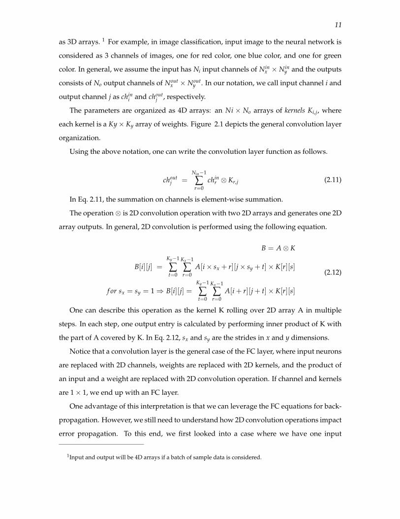
2.1 The organization of a CNN layer. . . . . . . . . . . . . . . . . . . . . . . . . . . . . . . . . . . . . . 12
4.1 Analog vector and matrix operations.(a) Using a bitline to perform an analogsum of products operation. (b) A memristor crossbar used as a vector-matrixmultiplier. . . . . . . . . . . . . . . . . . . . . . . . . . . . . . . . . . . . . . . . . . . . . . . . . . . . . . . . . 38
4.2 ISAAC architecture hierarchy. . . . . . . . . . . . . . . . . . . . . . . . . . . . . . . . . . . . . . . . . 39
4.3 Minimum input buffer requirement for a 6× 6 input feature map with a 2× 2kernel and stride of 1. The blue values in (a), (b), and (c) represent the buffercontents for output neurons 0, 1, and 7, respectively. . . . . . . . . . . . . . . . . . . . . . . 41
4.4 Example CNN layer traversing the ISAAC pipeline. . . . . . . . . . . . . . . . . . . . . . . 48
4.5 CE and PE numbers for different ISAAC configurations. H128-A16-C4 forbar I8 corresponds to a tile with 8 IMAs, 16 ADCs per IMA, and 4 crossbararrays of size 128×128 per IMA. . . . . . . . . . . . . . . . . . . . . . . . . . . . . . . . . . . . . . . 54
4.6 Normalized throughput (top) and normalized energy (bottom) of ISAAC withrespect to DaDianNao. . . . . . . . . . . . . . . . . . . . . . . . . . . . . . . . . . . . . . . . . . . . . . . 59
5.1 The ISAAC Architecture. . . . . . . . . . . . . . . . . . . . . . . . . . . . . . . . . . . . . . . . . . . . . 64
5.2 Microarchitecture of an IMA. . . . . . . . . . . . . . . . . . . . . . . . . . . . . . . . . . . . . . . . . . 67
5.3 Heterogeneous ADC sampling resolution . . . . . . . . . . . . . . . . . . . . . . . . . . . . . . . 68
5.4 Karatsuba’s Divide & Conquer Algorithm . . . . . . . . . . . . . . . . . . . . . . . . . . . . . . 70
5.5 IMA supporting Karatsuba’s Algorithm. . . . . . . . . . . . . . . . . . . . . . . . . . . . . . . . 71
5.6 Mapping of convolutional layers to tiles . . . . . . . . . . . . . . . . . . . . . . . . . . . . . . . . 73
5.7 Mapping layers to tiles for small buffer sizes. . . . . . . . . . . . . . . . . . . . . . . . . . . . . 74
5.8 Strassen’s Divide & Conquer Algorithm for Matrix Multiplication. . . . . . . . . . . 76
5.9 Mapping Strassen’s algorithm to a tile. . . . . . . . . . . . . . . . . . . . . . . . . . . . . . . . . . 76
5.10 Crossbar under-utilization with constrained mapping. . . . . . . . . . . . . . . . . . . . . 81
5.11 Impact of constrained mapping and compact HTree. . . . . . . . . . . . . . . . . . . . . . . 81
5.12 Improvement due to the adaptive ADC scheme. . . . . . . . . . . . . . . . . . . . . . . . . . 82
5.13 Comparison of CE and PE for Divide and Conquer done recursively. . . . . . . . . 82
5.14 Improvement with Karatsuba’s Algorithm. . . . . . . . . . . . . . . . . . . . . . . . . . . . . . 82
5.15 Buffer requirements for different tiles, changing the type of IMA and thenumber of IMAs. . . . . . . . . . . . . . . . . . . . . . . . . . . . . . . . . . . . . . . . . . . . . . . . . . . . 84
5.16 Improvement in area efficiency with decreased eDRAM buffer sizes. . . . . . . . . 84
5.17 Decrease in power requirement when frequency of FC tiles is altered. . . . . . . . 84
5.18 Improvement in area efficiency when sharing multiple crossbars per ADC inFC tiles. . . . . . . . . . . . . . . . . . . . . . . . . . . . . . . . . . . . . . . . . . . . . . . . . . . . . . . . . . . 85
5.19 Improvement due to the Strassen technique. . . . . . . . . . . . . . . . . . . . . . . . . . . . . 85
5.20 Peak CE and PE metrics of different schemes along with baseline digital andanalog accelerator. . . . . . . . . . . . . . . . . . . . . . . . . . . . . . . . . . . . . . . . . . . . . . . . . . . 86
5.21 Breakdown of area efficiency. . . . . . . . . . . . . . . . . . . . . . . . . . . . . . . . . . . . . . . . . . 86
5.22 Breakdown of decrease in power envelope. . . . . . . . . . . . . . . . . . . . . . . . . . . . . . 87
5.23 Breakdown of energy efficiency. . . . . . . . . . . . . . . . . . . . . . . . . . . . . . . . . . . . . . . . 87
x

LIST OF TABLES
4.1 ISAAC Parameters. . . . . . . . . . . . . . . . . . . . . . . . . . . . . . . . . . . . . . . . . . . . . . . . . . 50
4.2 Benchmark names are in bold. Layers are formatted as Kx ×Ky, No/stride (t),where t is the number of such layers. Stride is 1 unless explicitly mentioned.Layer* denotes convolution layer with private kernels. . . . . . . . . . . . . . . . . . . . . 53
4.3 Buffering requirement with and without pipelining for the largest layers. . . . . 55
4.4 Comparison of ISAAC and DaDianNao in terms of CE, PE, and SE. Hyper-Transport overhead is included. . . . . . . . . . . . . . . . . . . . . . . . . . . . . . . . . . . . . . . . 58
5.1 Key contributing elements in Newton. . . . . . . . . . . . . . . . . . . . . . . . . . . . . . . . . . 78
5.2 Benchmark names are in bold. Layers are formatted as Kx ×Ky, No/stride (t),where t is the number of such layers. Stride is 1 unless explicitly mentioned. . . 79

ACKNOWLEDGEMENTS
Before coming to the U.S. for my Ph.D., I lived all my life in Tehran, close to my family.
My parents selflessly encouraged me to leave for greater achievements, while they badly
want me to be there. Having them is one of the greatest blessings in my life. Their love
and support are far beyond what words can describe.
I was honored and privileged to have Rajeev Balasubramonian as my Ph.D. Advisor.
Not only did he teach me how to research, but he also taught me how to live and prosper.
I really appreciate his patience and support. 1
I would like to thank my Ph.D. committee, Al Davis, Erik Brunvand, Mahdi Bojnordi,
and Vivek Srikumar, for their feedback and support during my Ph.D. Moreover, I learned
life lessons from Al, critical thinking from Erik in the reading club, the basics of machine
learning from Vivek’s course, and the inspiration to always keep the bar high from Mahdi.
I would like to thank my mentor, Naveen Muralimanohar of Hewlett Packard Enter-
prise, who trusted me with doing research on in-situ computing, and other people at HPE
Lab that generously shared their invaluable knowledge with me.
To me, the main goal of the Ph.D. was to make great friends. This way, I can certainly
call my Ph.D. a success. When I came to Salt Lake City in 2012, I did not know anyone.
Five years later, I had many life-lasting friends. I would like to thank them all. I enjoyed
the time I spent with Uarch members, Ani, Kshitij, Nil, Seth, Manju, Sahil, Akhila, Arjun,
Chandru, Surya, and Karl. I would like to especially thank Anirban, Meysam, and Pey-
man, who helped me with my dissertation. I would like to thank many other friends, with
whom I shared a lot of great moments. 2 I am blessed with their friendship.
I would like to thank Karen, Ann, Robert, Leslie, Chethika, and other amazing people
at the University of Utah for their enormous support.
1and the ping-pong table.
2especially the surprise birthday celebration near the ISCA deadlines.

Although I specifically thanked a few people, I am fully aware and appreciate many
others who indirectly encouraged me, inspired me, or made this journey much easier for
me.
xiii

CHAPTER 1
INTRODUCTION
1.1 Computation Requirements of Deep Learning AlgorithmsThe field of Machine Learning helps develop computation models that learn the en-
vironment without explicit programming. The goal is to reach human intelligence and
beyond.
To this end, researchers have developed many models such as SVM (support vector
machine), decision trees, and regression.
One of the most promising models so far is artificial neural networks (ANNs). Inspired
by biological neurons, McCulloch and Pitts developed the first model of ANNs in 1943.
Later, at the end of the 1950s, a perceptron had been proposed, raising optimism about im-
minent human level intelligence [155]. However, in 1969, Minsky and Papert showed the
weaknesses of the perceptron model, which discouraged further activity in ANNs [128]. In
the 70s and 80s, backpropagation had been introduced and developed for training a neural
network from raw data. Later in the 90s, LeCun et al. proposed convolutional neural
networks (CNNs) leading to promising results in handwritten character recognition [103].
Even with the advent of CNNs, researchers were still relying on other approaches such
as SVM or ensemble of different models to achieve the best results.
The power of ANNs was revealed to researchers as the size of networks and training
data sets grew. Particularly, Alexnet was a milestone that won the ImageNet competition
in 2012 [96] by reducing the error rate by almost a factor of two, compared to other ap-
proaches. This work successfully trained a multimillion-parameter network with millions
of raw input images using back-propagations. Alexnet training took 6 days. Without a
high-speed GPU for training, Alexnet training would have taken much longer. In other
words, the computation power of today’s machines is a primary driver for major advance-
ments in the field of machine learning. Machine learning researchers have also developed

2
a number of techniques in the last decade to help deep networks learn, e.g., the use of
shared weights, dropout, expanded inputs, better activation functions, and regularization.
The Alexnet structure – a sequence of convolutional layers followed by fully-connected
classifier layers that is used for image classification – has also been used in many subse-
quent works and rejuvenated the field of deep learning. In deep learning, multiple non-
linear layers automatically extract and abstract features from raw data for different pur-
poses such as classification and prediction. The deeper layers in the networks combine
more simple features from the earlier layers to extract more complex features and rec-
ognize complicated objects in input images. Such deep neural networks (DNNs) have
recently achieved better results than human image classification. However, these out-
standing results are not for free; DNNs require billions of operations per image for the
simple task of classification. Figure 1.1 shows the top-1 accuracy and the computational
requirements for recent DNNs. In this figure, the trend suggests that more computation
leads to higher accuracy. In addition, the computational requirement grows significantly
with increase in the size of input, number of training samples, and the number of classifi-
cation categories. Therefore, providing faster machines is essential.
Deep networks have to be trained. The training currently takes many weeks across
several high-powered GPUs in a datacenter. Once the network is trained, it is deployed
on several devices (datacenter servers, self-driving cars, drones, mobile devices, etc.),
where it performs inference on billions of images every day. Faster machines are not only
essential for the training operations in deep networks, they are also essential for inference
operations. This dissertation focuses on both inference and training.
One promising solution to the computational requirements of DNNs is hardware spe-
cialization. It is well known that custom ASICs can be up to three orders of magnitude
faster than general purpose systems [69].
Since effective neural networks have always been computation-intensive, there have
been many prototypes and hardware architecture proposals.
Most of this prior work focuses on digital architectures, and we review some of them
in the background chapter. In this dissertation, we explore the use of analog units for
DNN acceleration and make some of the first contributions in the field of in-situ analog
computing for DNNs.

3
Figure 1.1. The classification accuracy vs. computation requirements (GOps) for theinference step in recent well-known image classifiers [25]. The circle around each pointdepicts the number of parameters.
To make the potential impact of this work clear, consider the following concrete use
case. Some modern cars (and likely most cars in the future) use a variety of cameras
and sensors to gather road/traffic information. Processing this information will require
computers that consume several hundreds of watts and precious space. The accelerators
defined in this dissertation will help process many more images (safety) with a computing
system that consumes tens of watts (energy efficiency) and fits under the seat of the car.
1.2 Dissertation OverviewMachine learning algorithms are a good candidate for specialization as they are em-
barrassingly parallel and require massive computation power. Most of the execution time
of these algorithms is spent on computing convolution and classifier layers. All of these
layers can be expressed as matrix-by-vector multiplications followed by a nonlinear acti-
vation. Machine learning algorithms also require a large set of parameters; much of the

4
time and power spent on these algorithms can be attributed to the high cost of moving
these parameters between memory and computational units.
1.2.1 Thesis Statement
We hypothesize that analog units have the potential to dramatically improve efficiency
for inference in machine learning accelerators because of their ability to perform in-situ
calculations and reduce data movement. We further hypothesize that clever management
of the ADC units will be vital in realizing the potential of in-situ computation.
1.2.2 ISAAC
A number of recent efforts have attempted to design accelerators for popular ma-
chine learning algorithms, such as those involving convolutional and deep neural net-
works (CNNs and DNNs). These algorithms typically involve a large number of multiply-
accumulate (dot-product) operations. A recent project, DaDianNao, adopts a near data
processing approach, where a specialized neural functional unit performs all the digital
arithmetic operations and receives input weights from adjacent eDRAM banks.
Chapter 4 explores an in-situ processing approach, where memristor crossbar arrays
not only store deep network parameters (the synaptic weights), but are also used to per-
form dot-product operations in an analog manner. No prior work has designed or char-
acterized a full-fledged DNN accelerator based on crossbars. In particular, our work
makes the following contributions: (i) We design a pipelined tiled architecture, with some
crossbars dedicated for each neural network layer, and eDRAM buffers that aggregate data
between pipeline stages. (ii) We define new data encoding techniques that are amenable to
analog computations and that can reduce the high overheads of analog-to-digital conver-
sion (ADC). (iii) We define the many supporting digital components required in an analog
CNN accelerator and carry out a design space exploration to identify the best balance of
memristor storage/compute, ADCs, and eDRAM storage on a chip. On a suite of CNN
and DNN workloads, the proposed ISAAC architecture yields improvements of 14.8×,
5.5×, and 7.5× in throughput, energy, and computational density (respectively), relative
to the state-of-the-art DaDianNao architecture.
5
1.2.3 Newton
Using ISAAC as a starting point, we then create a next-generation architecture, New-
ton, described in Chapter 5 of the dissertation. Newton addresses two significant short-
comings in ISAAC. First, ISAAC is a homogeneous design where every resource is provi-
sioned for the worst case. Second, the ADCs account for a large fraction of chip power and
area. By addressing both problems, Newton moves closer to achieving optimal energy-
per-neuron for crossbar accelerators.
We introduce six new techniques that apply at different levels of the tile hierarchy.
Two of the techniques leverage heterogeneity: one adapts ADC precision based on the
requirements of every subcomputation (with zero impact on accuracy), and the other
designs tiles customized for convolutions or classifiers. Two other techniques rely on
divide-and-conquer numeric algorithms to reduce computations and ADC pressure. The
final two techniques place constraints on how a workload is mapped to tiles, thus helping
reduce resource provisioning in tiles. For a wide range of CNN dataflows and structures,
Newton achieves a 77% decrease in power, 51% improvement in energy efficiency, and
2.2× higher throughput/area, relative to ISAAC accelerator.
1.2.4 Evaluation of Analog Architecture for Training
We also evaluate the potential of using an analog accelerator for training DNNs. We
show that due to three major weaknesses, analog accelerators are not as efficient as digital
ones for training. First, analog accelerator endurance is limited because today’s large data
sets cause millions of weight updates per training iteration. Second, analog accelerators
work with fixed point operators, which reduces the operation accuracy and consequently
increases the trained networks’ error rate. Finally, analog accelerators can only expedite
the forward and backward paths, but they require far more time for weight updates.
1.3 Layout of This DissertationThe rest of this dissertation is organized as follows. In Chapter 2, we explain the
computation requirement of DNNs in both inference and training phases. In Chapter 3, we
review the prior software and hardware-related work to accelerate DNNs. Chapter 4 and
Chapter 5 cover proposed architectures, ISAAC and Newton, respectively. We investigate

6
in-situ computing to accelerate DNN training in Chapter 6. Finally, Chapter 7 discusses
our primary conclusions.

CHAPTER 2
BACKGROUND
2.1 IntroductionIn this chapter we explain the computational requirements of deep neural networks
(DNNs). DNNs are built by connecting different layers of neurons serially or in parallel,
and they typically represent a direct acyclic graph (DAG) of computations. Depending on
the applications, one might leverage different types of layers. In this section, we review
some of the common layers, in both inference (forward path) and training phase (backward
error propagation). More specifically, we review both forward and backward paths for
fully-connected, convolution, pooling, sigmoid, and ReLU layers.
2.2 Computation FlowSince DNNs are DAGs, the flow of computation in the inference mode is straightfor-
ward. The input data is the first layer’s input and the output of each layer will serve as the
input for the next layer in the graph of computation. In the case of classification, the last
layer’s neurons can be interpreted as the predicted chance of one classes.
In the training mode, a pair of sample data and a label will be considered as the
input. Similar to the inference mode, DNN receives the sample data and generates a
vector of probability as its output. Then a loss function (also known as cost function)
evaluates the result by comparing it with the label. The goal of training is to reduce the
loss function. One can consider the entire neural network as one complex function. The
goal is to reduce the sum of the loss function output for all the training samples. Assume
S = {(xi, li) i ∈ {0, .., N − 1} } is the set of training samples with N members. Also
consider a neural network with M cascaded layers. We represent Layer i with a function
fi(x) and its parameters as W(i). Therefore, the output of the entire network, for the input
xi is
outi = fM−1(...( f2( f1(xi)))...) (2.1)

8
The loss value for this input is Loss(outi, li). The goal is to minimize the following
equation.
L =N−1
∑0
Loss(outi, li) (2.2)
There are multiple ways to solve this optimization problem. In the gradient descent
approach, in each step, L is calculated and W(i) are updated in a direction to get closer to
the local minimum. For the layer k, the i-th parameter is updated using the following rule:
W(k)i = W(k)
i − η × ∂L
∂W(k)i
(2.3)
In the above equation, η is the learning rate. Large η values lead to fast convergence at
the risk of missing some local minimum. On the other hand, small ηs do not jump over
optimum points at the cost of slower convergence.
The problem with gradient descent is that for every update step, we have to calculate all
outis. Therefore, the time for each step grows linearly with the training set size. As a result,
this technique is not used for large-scale DNNs in practice. Instead, stochastic gradient
descent will be applied. In this approach, the training set is shuffled and decomposed into
many small minibatches and gradient descent is applied to each minibatch. Therefore, the
number of outputs involved in each parameter update step is a function of the number of
elements in each minibatch. In practice, minibatches are much smaller than the training
set. The process of training all the minibatches is called an epoch. Since updating parame-
ters is based on a few samples in the minibatch, the training is carried for multiple epochs.
In each weight update step, we also need to calculate the gradient of each weight with
respect to the loss function. Applying the chain rule, we can find the gradient for the
functional representation of the neural networks (Eq. 2.1).
∂L
∂W(k)i
=∂L
∂yN−1× ∂yN−1
∂W(k)i
∂yM−1
∂W(k)i
=∂yM−1
∂yM−2× ∂yM−2
∂W(k)i
...∂yk+1
∂W(k)i
=∂yk+1
∂yk× ∂yk
∂W(k)i
(2.4)

9
In Eq. 2.4, yr is the output of r-th layer (outi = yN−1). This process is called backward
error propagation or backpropagation, where the loss error ∂L∂yN−1
is propagated in the opposite
direction of inference networks. In the backward network, the intermediate results of layer
t is et =∂L
∂yM−1−tand the parameters in the backward network are ∂yt
∂yt−1. We have,
∂L∂yt
=∂yt
∂yt−1× ∂L
∂yt−1
et =∂yt
∂yt−1× et−1
(2.5)
Therefore, one can rewrite gradient calculation in Eq. 2.4 as follows.
e0 =∂L
∂yM−1
e1 =∂yM−1
∂yM−2× e0
...
ek =∂yk−1
∂yk−2× ek−1
∂L
∂W(k)i
= ek ×∂yk
∂W(k)i
(2.6)
∂yk
∂W(k)i
depends on the input of Layer k (i.e., yk−1). In other words, in the process of weight
update both yis and eis are needed.
In the following part of this chapter we discuss the functionality of some of the most
popular layers.
2.3 Neural Network LayersIn this section we review some of the most popular layers deployed in deep learning
architecture.
2.3.1 Fully-Connected layer (FC)
This is the most used layer in the history of neural networks. In this layer, every output
neuron is the weighted sum of every input neuron (Eq. 2.7). The layer is illustrated as a
bipartite graph with one side representing input neurons while the other sides are output
neurons. In between any pair of input neuron, Ni, and output neuron, Mj, there is an
edge labeled with the weight wi,j. This layer can also be represented as a matrix by vector

10
multiplication W × N = M, where W, N, and M are the weight matrix, the vector of input
neuron values, and the vector of output neuron values, respectively. we have
Mj =n−1
∑i=0
Wi,j × Ni (2.7)
where n is the number of element input neurons. Similarly, we define m as the number of
output neurons. With the above notation, we can now derive the backpropagation rules
for FC layer.L
∂Ni=
m−1
∑j=0
∂L∂Mj
×∂Mj
∂Ni
L∂Ni
=m−1
∑j=0
∂L∂Mj
×Wi,j
(2.8)
if ein = [ L∂Ni
]0≤i<n and eout = [ L∂Mi
]0≤i<m are the input and output error vectors, we can
write:
ein = WT × eout (2.9)
where T is the matrix transpose operation. In addition to the error propagation, we have
to calculate the gradient of each weight with respect to the output layer.
∂L∂Wi,j
=m−1
∑t=0
∂L∂Mt
× ∂Mt
∂Wi,j
∂L∂Wi,j
=∂L
∂Mj×
∂Mj
∂Wi,j
∂L∂Wi,j
=∂L
∂Mj× Ni
(2.10)
As shown in Eq. 2.10, the gradient for the FC layer depends on the inputs and the
propagated error in the output.
FC layers requires m× n parameters, m× n multiplications and m× n additions.
2.3.2 Convolution Layer
In the FC layer, all input neurons have influence on all the output neurons, which
causes two problems: (i) the FC layer cannot preserve features that depend on the spatial
locality and (ii) the number of parameters and operations increase superlinearly.
Convolution Layer has been proposed to address these two weaknesses. In a convolu-
tion layer, input and output neurons are organized in an array of channels, each of which
are 2D arrays of input neurons. By this organization, the input and output are considered
11
as 3D arrays. 1 For example, in image classification, input image to the neural network is
considered as 3 channels of images, one for red color, one blue color, and one for green
color. In general, we assume the input has Ni input channels of Ninx × Nin
y and the outputs
consists of No output channels of Noutx × Nout
y . In our notation, we call input channel i and
output channel j as chini and chout
j , respectively.
The parameters are organized as 4D arrays: an Ni × No arrays of kernels Ki,j, where
each kernel is a Ky× Ky array of weights. Figure 2.1 depicts the general convolution layer
organization.
Using the above notation, one can write the convolution layer function as follows.
choutj =
Nin−1
∑r=0
chinr ⊗ Kr,j (2.11)
In Eq. 2.11, the summation on channels is element-wise summation.
The operation⊗ is 2D convolution operation with two 2D arrays and generates one 2D
array outputs. In general, 2D convolution is performed using the following equation.
B = A⊗ K
B[i][j] =Ky−1
∑t=0
Kx−1
∑r=0
A[i× sx + r][j× sy + t]× K[r][s]
f or sx = sy = 1⇒ B[i][j] =Ky−1
∑t=0
Kx−1
∑r=0
A[i + r][j + t]× K[r][s]
(2.12)
One can describe this operation as the kernel K rolling over 2D array A in multiple
steps. In each step, one output entry is calculated by performing inner product of K with
the part of A covered by K. In Eq. 2.12, sx and sy are the strides in x and y dimensions.
Notice that a convolution layer is the general case of the FC layer, where input neurons
are replaced with 2D channels, weights are replaced with 2D kernels, and the product of
an input and a weight are replaced with 2D convolution operation. If channel and kernels
are 1× 1, we end up with an FC layer.
One advantage of this interpretation is that we can leverage the FC equations for back-
propagation. However, we still need to understand how 2D convolution operations impact
error propagation. To this end, we first looked into a case where we have one input
1Input and output will be 4D arrays if a batch of sample data is considered.
12
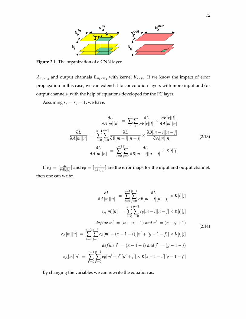
Figure 2.1. The organization of a CNN layer.
An1×n2 and output channels Bm1×m2 with kernel Kx×y. If we know the impact of error
propagation in this case, we can extend it to convolution layers with more input and/or
output channels, with the help of equations developed for the FC layer.
Assuming sx = sy = 1, we have:
∂L∂A[m][n]
= ∑r
∑t
∂L∂B[r][t]
× ∂B[r][t]∂A[m][n]
∂L∂A[m][n]
=x−1
∑i=0
y−1
∑j=0
∂L∂B[m− i][n− j]
× ∂B[m− i][n− j]∂A[m][n]
∂L∂A[m][n]
=x−1
∑i=0
y−1
∑j=0
∂L∂B[m− i][n− j]
× K[i][j]
(2.13)
If eA = [ ∂L∂A[i][j] ] and eB = [ ∂L
∂B[i][j] ] are the error maps for the input and output channel,
then one can write:
∂L∂A[m][n]
=x−1
∑i=0
y−1
∑j=0
∂L∂B[m− i][n− j]
× K[i][j]
eA[m][n] =x−1
∑i=0
y−1
∑j=0
eB[m− i][n− j]× K[i][j]
de f ine m′ = (m− x + 1) and n′ = (n− y + 1)
eA[m][n] =x−1
∑i=0
y−1
∑j=0
eB[m′ + (x− 1− i)][n′ + (y− 1− j)]× K[i][j]
de f ine i′ = (x− 1− i) and j′ = (y− 1− j)
eA[m][n] =x−1
∑i′=0
y−1
∑j′=0
eB[m′ + i′][n′ + j′]× K[x− 1− i′][y− 1− j′]
(2.14)
By changing the variables we can rewrite the equation as:
13
epadB [m][n] = e[m− x + 1][n− y + 1] = e[m′] i f m ≥ x− 1 n ≥ y− 1
otherwise ⇒ epadB [m][n] = 0
Also de f ine K′[i][j] = [x− 1− i][y− 1− j]
eA[m][n] =x−1
∑i′=0
y−1
∑j′=0
eB[m′ + i′][n′ + j′]× K[x− 1− i′][y− 1− j′]
eA[m][n] =x−1
∑i=0
y−1
∑j=0
epadB [m + i][n + j]× K′[i][j]
eA = epadB ⊗ K′
(2.15)
In other words, error map in the input channel is the convolution of output channel
error maps that has been padded with zeros (i.e., epadB ) with the rotated version of the
original kernel (i.e., K′).
In general for Ni input channels and No output channels, we have:
echini=
No−1
∑j=0
epadchout
i⊗ K′i,j (2.16)
Similarly, the weight update array for kernel Ki,j is calculated as follows:
∂L∂Ki,j
= epadchout
j⊗ chin
i (2.17)
In general, we can state that both forward and backward operations are convolutional
operations. The number of parameters in this layer is No × Ni × Kx × Ky and the number
of operations for additions and multiplications No × Noutx × Nout
y × (Ni × Kx × Ky).
2.3.3 Pooling Layer
As we mentioned, the number of operations in the convolution layer depends on the
size of channels. A pooling layer is proposed to down-sample output channels of the
convolution layers. A pooling layer is applied per channel. Therefore, it preserves the
number of channels in the input. However, the output channels have smaller dimensions.
There are two common types of pooling layers, average pooling and max pooling. Average
pooling is a 2D convolution operation of Kernel KKx×Ky with all its weights equal to 1Kx×Ky
.
Max pooling, on the other hand, is a 2D convolution with Kernel 1Kx×Ky that uses max
operation instead of addition. It is also worth noting that the strides in pooling layers are
typically greater than one to reduce the dimensions of the resulting output channels.

14
Since the average pooling is essentially 2D convolution, we can apply Eq. 2.15 to cal-
culate its error maps. For max pooling, error in the output is just propagated to the input
with the maximum values.
When a pooling layer with kernel of size Kx × Ky kernel and strides of size sx and sy is
applied to Ni input channels of size Nx × Ny, Nx×Ny×Kx×Kysx×sy
operations are required.
2.3.4 Nonlinear Layers
The secret ingredient in DNNs is nonlinearity. Without nonlinear layers, DNNs are
simply a polynomial function of input values. There are three types of nonlinear layers;
sigmoid, tanh, and ReLU. These functions are represented by the following equations:
σ(x) =1
1 + e−x
tanh(x) = 2σ(2x)− 1
ReLU(x) = max(0, x)
(2.18)
Many recent DNNs have adopted ReLU due to its simplicity and high accuracy. How-
ever, sigmoid and tanh are still used in LSTMs (Long Short Term Memory). Additionally,
some work suggests to approximate the exponential operator in sigmoid and tanh with
piece-wise linear functions [28].
Although sigmoid and tanh have exponential operators, they are simply differentiable
based on the forward path values.
∂σ(x)∂x
= σ(x)(1− σ(x))
∂tanh(x)∂x
= (1 + tanh(x))× (1− tanh(x))
∂ReLU(x)∂x
=
{1 if x ≥ 00 if x < 0
(2.19)
2.4 ConclusionIn this section, we reviewed common layers used in state-of-the-art DNNs. We showed
that computation intensive layers such as convolutions and FC have the same type of
operations in both forward and backward paths.

CHAPTER 3
RELATED WORK
3.1 IntroductionIn this chapter, we review some of the previous work that aims to simplify DNN
programmability or acceleration. We first review software solutions for CPUs and GPUs
on datacenters or mobile platforms (Section 3.2). Then, we review both analog and digital
hardware implementations of DNNs (Section 3.3). Finally, we conclude this chapter in
Section 3.4.
3.2 Software ApproachThere are multiple software approaches to accelerate DNNs. In this section, we catego-
rize them into four groups. In the first two subsections, we review software solutions for
CPU-based and GPU-based platforms. Then we list some of the popular Deep Learning
frameworks that simplify DL programming. Some of these frameworks are also able to
distribute DNNs over multiple machines. Finally, we look into approximation approaches
that aim to reduce the number of operations without a loss in accuracy.
3.2.1 Software Optimization for CPUs
Matrix-by-vector multiplication, or MVM, is the key operation in DNNs. Therefore, it
is possible to take advantage of efficient linear algebra libraries to accelerate these algo-
rithms. The de-facto standard for linear algebra is BLAS (Basic Linear Algebra Subpro-
gram), which is a set of function specifications commonly used in linear algebra. Libraries
such as OpenBlas [142], ATLAS [15], Intels MKL [130] are the implementations of the BLAS
interface. ATLAS (Automatically Tuned Linear Algebra Software) is a library that tunes its
parameters based on the host hardware. MKL (Math Kernel Library) takes advantage
of Intel AVX (Advanced Vector Extension) instructions and Intel SSE2 code to optimize
operations such linear algebra, FFT (Fast Fourier Transform), statistics, and PDEs (Partial

16
Differential Equations).
Besides BLAS, Eigen [53], a C++ template library,l is also used for linear algebra oper-
ations. This library is designed to be versatile, fast, and reliable. Depending on the host, it
tries to take advantage of available vector instructions (e.g., Intel AVX, ARM NEON, and
PowerPC AltiVec).
Other libraries such as Blaze [21], Armadillo [161], UBLAS [2] by Boost, and (Matrix
Template Library) MTL [185] are also used for linear algebra. However, they are not that
popular among DL frameworks compared with others mentioned earlier.
In addition to dense Linear Algebra, some DNNs rely on sparse MVMs; popular sparse
libraries for CPUs are Intel MKL and ViennaCL. Augusto et al. compare these algorithms,
in terms of performance , and report the superiority of Intel MKL in terms of performance
[16].
There have been some comparisons between different techniques and code optimiza-
tions for DNNs on CPUs. Vanhoucke et al. use a speech recognition algorithm and show
that memory layout, batching and clever usage of SSE2 and taking advantages of fixed-
point instructions in SSE3 can improve performance by 10x [186]. Cong and Xia propose
optimized matrix multiplication operations to reduce the number of CPU operation by up
to 47% [40].
Rajbhandari et al. characterized the GEMM (General Matrix Multiply) operations (i.e.,
GEMM-in-Parallel and Parallel-GEMM) for CNN on CPU and proposed an optimization
framework that generates optimized sparse codes as well as a scheduler based on GEMM-
in-Parallel citerajbhandarihe17.
Besides the works focusing on CPU side optimization, there are works to reduce the
memory footprint for CNN while running on a CPU. More precisely, Matveev et al. showed
how to run connectomics 1 application on small multicore machines (with less than 100
cores) rather than a huge cluster of CPUs and GPUs.
3.2.2 Software Optimization for GPUs
As we mentioned, DL algorithms rely on linear algebra significantly. Due to their
SIMD (Single Instruction stream Multiple Data stream) architectures, GPUs are excellent
1Connectomics is a field of studying brain’s connection by image processing of brain images.

17
fits for such applications. In SIMD architecture, one stream of control instructions instructs
multiple functional units, which enable power-efficient massive parallel programming. In
addition, GPUs allocate most of their real estate to ALUs rather than on-chip caches. In
this section, we look into some of the GPU primitives used and customized for DNNs.
As we mentioned, DNNs rely on linear algebra functions. cuBLAS is the CUDA imple-
mentation of BLAS specification. ViennaCL is an openCL based library, which is able to
run on CPUs, GPUs, and Xeon Phis. It can outperform cuBLAS in sparse matrix multipli-
cations. MAGMA is a library for linear algebra with the goal of achieving fast implemen-
tation on hybrid/heterogeneous architectures.
There are also Python modules and wrappers for basic linear algebra primitives. Gnumpy
[181] and CudaMat [131] are two examples. Gnumpy provides a GPU implementation
for the popular Numpy Python library. Cudamat enables running CUDA kernels from a
Python script. The combination and these two libraries can provide a simple environment
for DNN development.
cuDNN is a library for DNNs built on Nvidias GPU [33]. It is also serves as a set
of function specifications for DL basic functions. cuDNN provides an implementation of
batched convolution optimized for specific GPU with respect to convolution layer param-
eters. cuDNN has been integrated into Caffe framework and leads to 36
Similar to cuDNN, AMD Radeon, another major GPU card vendor, has also provided
a DNN framework. AMD takes advantage of Berkeley Caffe and replaced its CUDA code
with its own HIP code [10].
In addition to running convolution in the time domain, one can perform it in the
frequency domain [124], [187]. In the frequency domain, convolution is translated into
element-wise multiplication. Lavin and Gray used the Winograd algorithm to reduce the
number of multiplication in the FFT-base implementation of convolution layer [99]. In
addition to CNN layers, there are works accelerating other layers on GPUs. For example,
Ly et al. proposed a solution to run RBMs (Restricted Boltzmann Machines) on the GPUs
[118]. There are also some projects targeting scalability by running DNNs over multiple
GPUs. dMath provides a library to run linear algebra algorithm in multiple possibly
heterogeneous GPUs [55]. Coates et al. used a cluster of GPUs to train a network with
more than 11 billion parameters [37]. Hauswald et al. proposed DjiNN a WSC (Warehouse
18
Scale Computer) service for DL networks [71]. They have also shown that WSCs enabled
by GPU can improve TCO (Total Cost of Ownership) by up to 40x compared to CPU-only
WSCs.
vDNN addressed the memory limitation on GPUs for training mode [154]. GPUs rely
on low-capacity but high bandwidth memory such as GDDRs and HBMs. However, train-
ing DNNs requires a huge amount of memory to store weights updates. vDNN virtualized
CPU-side high capacity memory for the GPUs. vDNN achieves this by using a software
prefetching scheme that delivers each layer’s variables when they are needed. vDNN
removes the memory capacity barrier with less than 18% performance loss compared to
expensive high-capacity GPUs.
3.2.3 Deep Learning Frameworks
On top of the library for CPUs and GPUs, researchers developed a framework to sim-
plify modeling and programming a new DL network. In this section, we review some of
these frameworks.
Theano is a Python library for the multidimensional array which runs on both CPUs
and GPUs and is particularly used for DNNs [12]. Developed at the University of Mon-
treal, Pylearn2 is a DL library built on top of Theano [65]. Alex Krichevsky developed
cuda-convnet, a fast c++/CUDA for DL networks and is scalable to multiple GPUs [96].
Zlateski et al. introduced ZNN, a large scale framework for shared memory system for
CPU architectures. Caffe is another DL framework that targets speed and modularity
[210]. Caffe supports both CPUs and GPUs and can run on top of cuDNN. Caffe supports
varieties of layers, loss functions, weight update optimizations. Ristretto is built on top
of Caffe to provide fixed point weights and to optimize the precision of these weights
[68]. The industry has also contributed to the field by releasing their DL frameworks.
Preferred Network America introduced Chainer that takes advantage of define-by-run
paradigm. More specifically, Chainer memorizes the computational graph during the
forward path and then uses this knowledge for the backward path of training [182].
Facebook also made its DL framework, Torch, available to the public. Torch provides
an efficient implementation of neural network layers on both CPUs and GPUs. It also
provides a high-level abstraction to these layers via C, Lua, and Python interfaces [39].

19
The other popular framework is Google's TensorFlow developed by Google Brain Team
[4]. TensorFlow looks in the DNNs as graphs of computation. TensorFlow is able to
run on a variety of platforms ranging from mobile devices to high-end GPUs. Intel also
provides software for DL development. Intel Nervanas framework Neon is one example
[136]. Neon outperforms most of the above frameworks for most of the layers used in DL
algorithms [1]. Microsoft also introduced its CNTK (Cognitive ToolKit). Microsoft claims
up to 10x speedup on recurrent neural networks compared with Google's TensorFlow
[183]. Microsoft also embedded many innovative schemes for scalability of its framework,
particularly in training mode.
Shi et al. compared some of these popular DL frameworks for different types of net-
works and on different hardware [167]. They have found that in many of these frame-
works the benefits of scaling from 4 CPU cores to 16 cores is marginal. In addition,
they found that Caffe, TensorFlow, and CNTK work the best for CNNs, fully connected
Networks, and RNNs, respectively.
There are also some projects that specifically target scalability. BigDL is DL framework
that distributes high-level model, written in Python and Scala, over Apache Spark cluster
[20]. MXNet supports four front-end languages (i.e., Python, R, Julia, and Go) and runs
on both GPUs and CPUs [135]. For GoogleNet network, it shows superlinear speedup.
Before launching TensorFlow, Google deployed DistBelief for its large-scale projects. This
framework supports an asynchronous stochastic gradient descent, named downpour SGC,
for distributed training [45]. Microsoft also launched Project Adam, a distributed system
for training very large DL networks. Adam balances the load over different components
of the system to achieve an efficient implementation [35]. Twitter showed a machine
learning software in their Hadoop-based platform [108]. SparkNet and DeepSpark are two
frameworks for DL algorithms training over Spark, which is a MapReduce like distributed
platform [87]. Cui et al. introduced GeePS that facilitates training on multiple GPUs that
can accelerate single-GPU training by 9.5x with 16 GPU machines [43]. Neurosurgeon is
a new tool that looks into the cloud-only processing of DL algorithms (e.g., Apple Siri and
Google Now) from mobile applications [83]. It provides a computation partitioning over
both cloud and mobile devices to optimize latency and energy consumption.

20
3.2.4 Approximation Approach
In the prior section, we reviewed prior works that try to manage the underlying hard-
ware for running DNNs more efficiently. In this section, we look into a new category
of works that approximate a network such that it requires less computation, demands
lower memory bandwidth, or occupies smaller capacity. There are multiple approaches to
reducing the computation of DL networks as described in the following subsection.
3.2.4.1 Compression
Memory capacity and bandwidth are the key performance and power bottlenecks of
DNNs. Although hardware lossless compression mechanisms can seamlessly reduce this
pressure, software solutions can outperform them [164]. To this end, software solutions
might retrain the network to adjust for the loss due to compression. In addition, software
solutions are superior as a DNN runtime is deterministic and does not need dynamic
solutions based on predictions. Here we review some of these software approaches. Deep
Compression showed that on top of its other techniques to reduce redundancy, Huffman
coding can boost compressibility from 31x down to 49x [166]. Ko et al. proposed a JPEG
encoding for the neural network weights. Their approach adjusts the level of quantization
based on the error sensitivity of the weights [94]. Koutnik et al. reduce the number of
parameters to learn in RL (reinforcement learning) algorithms by converting the weight
matrix into the frequency domain and removing high-frequency values [95]. To improve
their approach wavelet-based coding weights in the frequency domain have also been
proposed [85].
3.2.4.2 Pruning
Another approach to removing the DNN redundancy is to prune weights. Le Cun et al.
proposed optimal brain damage (OBD) as an automatic network minimization technique
for better generalization of a network with fewer training samples [104]. OBD tries to
remove weights that would affect the error rate during training mode the least. Their
approach reduces the number of weights by a factor of two. Collins and Kohli showed
that using regularizer that promotes sparsity can reduce the number of weights by 4x with
around 2% reduction in the accuracy [38]. Liu et al. demonstrate sparse decomposition
to reduce unnecessary weights using their efficient implementation of sparse networks,

21
SCNN (Sparse CNN). They reported less than 1% reduction in the accuracy for removing
90% of the weight [110]. Han et al. proposed pruning followed by retraining to reduce the
weights overhead by up to 13x without any loss in the network accuracy [70]. Guo et al.
proposed an on-the-fly approach to prune connections that outperforms prior approaches
both in compression rate and the number of pruning-training iterations [66]. Liu and
Turakhia showed that by pruning of weights in the frequency domain, one can reduce the
number of weights by up to 90% in LeNet [116]. Later, researchers proposed structured
sparse networks to be more compatible with sparse matrix representation format. Lebedev
and Lempitsky proposed a group-wise version of OBM that reduces the operation to
smaller but dense matrices [102]. Wen et al. proposed SSL (Structured Sparsity Learning),
an approach to make the sparse networks both compact and hardware-friendly [192].
With the same premise, Anwar et al. also showed that intrakernel sparsity with strides
can reduce the redundancy dramatically [14]. Mao et al. observed that coarse-grain
sparsity is both more hardware-friendly and compressible compared to fine-grain sparsity.
In their work, they investigate the tradeoff between granularity and network accuracy
[121]. Finally, Han et al. showed that sparsity can improve the accuracy of dense networks
by up to 4.3%. To this end, they trained the network three times one as a dense network,
then as a sparse one and again as a dense one. In the last dense training, they returned
back the removed sparse weights and initialized them to zero [166].
3.2.5 Clustering
The other way to reduce the network redundancy is to cluster similar parameters to-
gether and replace all of them with one parameter. Nowlan and Hinton proposed a regu-
larization to shape the networks such that the distribution of weight values fits into multi-
ple Gaussians. Then they clustered similar weights. In their approach, clustering happens
during training [139]. HashedNet implemented clustering by grouping the weights using
hash functions. It then allocates one parameter to all the weights colliding to the same
bucket [29]. BHNN structured the hashing mechanism to providing spatial locality for
computation and hardware-friendliness while achieving 10x compressibility [208]. A sim-
ilar idea to HashedNet has been proposed in FreshNets to cluster weights in the frequency
domain representation [30]. Deep Compression applied weight sharing by categorizing
22
weights in multiple bins and allocating one value to all of them [166]. DivNet used
determinantal point process (DPP) for each layer to model the diversity of neurons. The
diversity is used then as a metrics to categorize similar neurons [123].
3.2.5.1 Matrix Reparametrization
Matrix reparametrization is a matrix approximation technique to reduce the capacity
and computation requirements of matrix operations. In this approach, one large matrix
is decomposed into the product of multiple smaller ones. Danil et al. discovered that
deep learning networks are over-parameterized. They showed that with only 5% of the
weight, one can predict the rest of them, accurately [46]. Inspired by this work, Gong
et al. factorized weight matrix using singular-value decomposition [64]. They achieved
up to 24× compression with no more than 1% loss in accuracy. Zhang et al. proposed an
optimization solution to minimize the reconstruction error for nonlinear layers subject to
lower number ranks, which leads to 4× speedup with only 0.9% loss in accuracy [204].
Jaderberg et al. reshape the CNN layers by decomposing its 2D filters into 1D filters
and achieved 2.5× and 4× speedup with no loss and 1% loss in accuracy, respectively
[78]. Similarly, Denton et al. proposed a low-rank solution with 2x speedup and 1%
accuracy loss [47]. They used a low-rank approximation that minimizes the distance
between the original and constructed matrices. To this end, they introduced a new metric
that magnifies error-sensitive weights more than others. Similarly, a CP-decomposition (
Canonical Polyadic decomposition) has been proposed with the same speedup-accuracy
loss tradeoff [101]. Deep Fried Convnets targeted the huge fully-connected layers and
uses adaptive Fastfood transform to reduce the number of parameters from O(nd) to
O(n) where d and n are the numbers of input and output neurons in a fully-connected
layer. In the Fastfood transform, the Matrix W representing FC-layer will be approximated
with SHGPHP where S, G, and B are diagonal matrices, P is a random permutation
matrix, and H is the Walsh-Hadamard matrix, respectively. Novikov et al. show a matrix
tensorization approach that reduces the FC-layer capacity by five orders of magnitudes
at the cost of 2% loss in accuracy. In this approach, the original matrix is reshaped into
a multidimensional tensor. Each element of the tensor is a product of multiple small
matrices [138]. Using the same concept, Garipov et al. extended ternsorizing for the entire

23
network and achieved 80× compression. The similar concept used in [18] to provide
a lookup-based CNN. Besides decomposition to smaller matrices/vectors, Sindhwani et
al. proposed using structured matrices. In these matrices, a few values repeat in multiple
entries. Using displacement operators, it is possible to transform such matrices to low-rank
ones [169].
3.2.5.2 Quantization
The quantization of DNN weights has been considered to simplify hardware accel-
eration. Feisler et al. used quantization for optical neural networks since the number
of intensity level in optics were limited to a few levels [59]. At the cost of the loss in
accuracy, they considered a set of integer values for the weights in each layer. Xie and
Jabri took advantage of a statistical quantization model (i.e., quantization as an error to
the real value) to investigate the effect of the number of bits, the number of layers on the
error due to quantization [195]. Based on their findings, they later proposed a combined
search algorithm which has two parts: Modified Weight Perturbation (MWP) and Partial
Random Search (PRS). MWP uses gradient check to find the direction of updating while
PSR adds randomness by randomly changing a weight value if it leads to a smaller error.
With these techniques, they achieved the same accuracy as the unlimited precision with
only 8-bit to 10-bit fixed point number representations [196]. Tand and Kwan quantized in
three phases: training, quantizing, and adjusting. In the quantizing phase, they just limited
the weight to be zero or a powers-of-two. Later in the adjusting phase, they minimized the
error by tuning the slope of the activation functions. In their evaluations, they could reduce
the number of values per weight to six numbers with no more than 3% accuracy loss [180].
Dundar et al. improved prior statistical models used by considering nonlinearity in their
model [52]. Draghici and Sethi theoretically showed the capability of integer weights for
classification [50] [49]. Alippi and Briozzo extended prior works on the accuracy loss
analysis due to quantization to cover cases with low fan-in neurons such as sparse NNs
[8]. Based on the interval arithmetic, Anguita et al. proposed a method to derive the
worst-case error due to quantization [13]. In their analysis, they considered a quantized
number as an interval around the real value and the size of the interval is assumed to be
the quantization error. This consideration made their approach independent of the input
24
data distribution.
All the abovementioed works investigated quantization for MLP. Since DNNs demand
high computations, quantization has also reapplied in the recent years. Hwang and Sung
used a backpropagation-based training to compress the weights to three cases (-1,0,+1). For
MNIST and TIMIT dataset, they observed a negligible loss in the accuracy [77]. To reduce
the overhead of multiplications in DNNs, Courbariaux et al. proposed a low-precision
training solution for fixed point, floating point and dynamic fixed point operations [41].
In their approach, they used low-precision operations during the forward and backward
propagations while using high-precision operations for updating the weights. For the
maxout network, they found that 10 bits per weights are enough. Gupta et al. observed
the critical role of rounding in low-precision fixed-point DNNs [67]. In their work, they
replaced the round-to-nearest approach with the stochastic rounding. In the stochastic
rounding, the distance between a floating point number and its fixed point neighbors are
used as a probability to round the floating point number to one of two neighbors. For
floating point numbers outside the boundary of the fixed point range, they assigned the
corresponding fixed point bound [90]. They proposed BNN (Bitwise Neural Networks)
with binary and ternary weights [109]. In their approach, based on the observation that
activation values are less sensitive to the error than the gradients, they considered floating
point gradient and power-of-two activation values for backpropagation. Lin et al. have
proposed a binary neural network derived from a real-valued one. The real-valued NN's
weights are restricted to [-1,+1] using tanh function. In their approach, they zeroed some
connections and the number of zeroed connections is a hyper parameters. XNOR-net
approximated a weight matrix as a product of some trainable floating point quotient and
a bipolar matrix. They minimized the error between the original matrix and the approxi-
mated one by assigning the sign value of the original weights to the binary matrix's entities
and the average of the weights value to the matrix quotient. BNN or (Binarized Neural
Networks) has been proposed to take advantage of hard sigmoid function, which is a
stochastic sign function for stochastic binarization of the weights. To avoid gradients
vanishing, they used straight-through estimator [42]. Miyashita et al. [129] used a
logarithmic representation of weights and activation function outputs. The logarithmic
representation can reduce the multiplication operations to shifts and adds. They also

25
showed a simple approximation for adding logarithmic values. TWN (Ternary Weight
Networks) approximated the original weight matrix with the product of a ternary matrix
and a floating point quotient. They proposed to find ternary weights by optimizing the
Euclidian distance of the original and the approximated matrices [106]. TTQ (Trained
Ternary Quantization) used ternary weights and two floating point quotients (Wn and Wp)
[206]. the entities with the value -1(+1) are multiplied by Wn(Wp). They also considered
a trainable threshold Wt for quantizing weights to -1, 0, and +1. DoReFa-Net proposed a
general framework with different precisions for the weights, activation values, and gradi-
ents [205]. With a negligible additional error, they trained AlexNet with 6-bit gradients.
3.2.6 Summary
We review many software approaches for the efficient implementation of DNNs. We
believe that the approximation techniques presented so far can also be applied to our
in-situ computing accelerators (discussed in Chapter 4 and 5). Furthermore, we think
that, with the emergence of hardware accelerators in the future, the software frameworks
reviewed here will be very helpful to program and manipulate these hardware units.
3.3 Hardware ApproachThe neural networks, compared to many other machine learning solutions such as SVM
(support vector machine), are computation intensive. As a result, there have been many
hardware acceleration proposals for neural networks. In this section, we review some of
these implementations for Digital ASICs, FPGA, and Analog ASICs.
3.3.1 Digital ASICs
Treleaven et al. [184] covered some of the earlier work on the hardware implementa-
tion of neural networks such as Netsim [176] and WISARD for image recognition. Nord-
strom and Svensson looked into a different way to parallelize large neural networks and
concluded that a ring-based network of SIMD architectures can achieve high utilization
[137]. Holi and Hwang offered a theoretical analysis to find the best precision for fixed-
point neural network implementations [75].
In the last few years, DNNs have shown dramatic accuracy improvement in many ap-
plications. This motivated many new implementations for neural networks. Chakradhar

26
et al. [27] proposed a coprocessor that reconfigures based on the available memory band-
width to optimize the throughput for CNNs. They also proposed a high-level abstraction
for neural networks to simplify accelerator programming. Kim et al. showed an ASIC
implementation of a multiobject recognition system [88]. Using a neural network, this
design finds the region of interest in the image and extracts the objects in those regions.
Finally, it matches the result with a database of objects. They reported more than 200
GOPs and real-time object recognition with 60 frames per second. Convolution Engine
[150] showed that multiple image processing tasks such as SIFT (Scale Invariant Feature
Transform) have 1D or 2D convolution access patterns. These tasks differ only in the oper-
ator involved in the convolution. Based on this observation, they proposed a coprocessor,
abstracted through a few function calls, for such general form convolution operations.
They reported that this Convolution Engine achieved more than 8× energy efficiency com-
pared to SIMD architectures. Gokhale et al. [63] presented nn-X, a low-power coprocessor
for ARM cores that achieves 227 GOPS in less than 4W. This architecture has multiple
simple processing units consisting of a convolution engine, a pooler, and a programmable
nonlinear function. These units are connected through an on-chip network. DianNao
[28] is a hardware accelerator with simple high-level instructions. To implement a neural
network, DinaNao uses NFU (Neural Functional Unit) that has three pipeline stages: the
multiplication stage, the addition stage, and the nonlinear function stage. The first two
layers perform a matrix-by-vector multiplication, while the last stage is used to realize
nonlinear activation function. DianNao achieves 452 GOPs in less than 500 mW while
occupying around 3mm2. Although DianNao is very area and power efficient, it requires
lots of data transfer for large neural networks. To solve this problem, DaDianNao has been
proposed. DaDianaNao tries to keep the kernel values on the chip to save the memory
bandwidth [32]. To this end, authors proposed to allocate 36 MB of eDRAM on the
chip; 32MB eDRAM on 16 Tiles and 4MB eDRAM in the center for input/output values as
well as the interchip communications. DaDianNao used a modified version of DianNao's
NFUs that are connected through a tree topology. DaDianNao outperforms a single GPU
by more than 450x while reducing the energy by 150×. ShiDianNao was another work
that improved DianNao [51]. ShiDianNao specifically targeted image applications and
proposed a mesh of ALUs to reduce the number of data transfer for CNNs. In addition,

27
ShiDianNao proposed to shift the accelerator next to the sensor to eliminate data transfer
between the sensor and DRAM. Using these two techniques, ShiDianNao achieved 60x
energy efficiency compared to DianNao. PuDianNao extended DaDianNao to support a
larger family of machine learning techniques [112]. More precisely, PuDianNao used a
modified version of DianNao's NFU to cover the most important machine learning tasks
such as linear regressions, k-means, k-nearest neighbors, and support vector machines.
PuDianNao improves energy efficiency by more than 128× compared to a K20M GPU.
Origami is another work that is scalable to TOPs performance in a limited power and
area envelope [26]. In this approach, authors used an image window logic that stores the
next sub-images required by the convolution units. For scalability, they also suggested
an FPGA-based system to distribute neural network weights between different Origami
chips. By reducing the weights to binary values, YodaNN [11] achieved more than 60
TOPS/Watt in 1.9mm2 area. Similar to ShiDianNao, Eyeriss has been proposed [31] to take
advantage of spatial locality in the CNN calculation using a systolic architecture. Eyeriss
explored the design space of such spatial architectures and proposed an approach to map
and schedule weights to such architectures [31]. Eyeriss improved the performance of
systolic architectures for large batch size by up to 2.5×. Lu et al. explored the CNN
access pattern and proposed FlexFlow [117]. FlexFlow uses a 2D mesh of processing
elements to parallelize DNNs. It tries to use different combinations of parallelism to
fully utilize its units. TETRIS extended Eyeris for a 3D memory system and improved
performance and energy efficiency by 4.1× and 1.5×, respectively [61]. Another work that
considered 3D memory is NeuroCube [86]. This approach used 3D memory technology
for a large number of weights in deep neural networks, especially the ones for scene
labeling. Azarkhish et al. also proposed Neurostream, an HMC-based process-in-memory
architecture for DL algorithms [17]. Their approach is scalable to multiple HMCs and
achieves 240 GFlOPS in 2.5W power budget.
Some of the prior work focused on making hardware acceleration more efficient. Cn-
vlutin [5] observed that many neural network's values are zero as many of them used
ReLU for activation function. They modified DaDianNao to filter out operations with
at least one zero operand. Minerva showed a high-level synthesis approach for DNN
accelerators [44]. It took advantage of the near-zero values for pruning as well as low-
28
voltage SRAM buffer to provide 8× power reduction with respect to the nonoptimized
baseline accelerator. Judd et al. observed that different layers of a network require different
numerical precisions and proposed Stripes [81]. This approach used bit-by-bit operations
to tune the number of bits needed per layer. EIE and SCNN used sparsity to reduce the
number of operations, for the fully-connected layer and convolutional layer, respectively
[165] [144]. In addition, EIE used clustering to reduce the numerical precision. Ren et al.
[153] suggested SC-DCNN, an architecture that uses stochastic computing to reduce the
power and area overhead of accelerators. In this approach, numbers that are represented
between [-1,1] will be represented by a stream of 1s. SC-DCNN achieves more than 500K
images/J for the MNIST benchmark.
There are also some recent works focusing on the training phase of DL algorithms.
Cambricon investigated the training phase [113] and identified the computation intensive
operations. They designed an architecture that supports three types of operations: scalar,
vector-based, and matrix-based. They achieve more than 3× improvement over GPU in
terms of performance. In ScaleDEEP, authors used heterogeneous process, smart mapping
of the weights, and a three-level interconnect to optimize the data transfer. They achieve
up to 28× speedup compared to a GPU implementation with the same power budget
[188]. TPUs (Tensor Processing Units) have recently been deployed by Google in its dat-
acenters. They have a systolic architecture with 256 × 256 8-bit ALUs. These units are
installed in PCI slots and controlled by the CPUs [80]. Depending on the memory type,
TPU can achieve between 15× to 70× power efficiency, compared to state-of-the-art GPUs.
3.3.2 FPGA
FPGAs (Field Programmable Gate Arrays) are hardware that can be reconfigured for
specific purposes. While FPGAs are not as efficient as ASICs, they reduce the cost of
acceleration, in terms of development cost, dramatically. Additionally, they can be reused
for many purposes; hence many applicants with different tasks can share them. In this
section, we review some of the prior works that have taken advantage of FPGA for neural
network acceleration.
Lysaght was the first to prototype an artificial neural network on an Atmel AT6005
FPGA [119]. In their implementation, they time-multiplexed different layers to cover
29
large-scale neural networks. Since then, there have been many FPGA prototypes. Zhe
et al. surveyed some of these works from the late 90s until 2005 [207]. In 2006, Deep
Belief Network was introduced which relied on RBMs (Restricted Boltzmann Machines).
Kim et al. showed an implementation for the training of an RBM network using 16-
bit arithmetic units, which leads to 25-30× performance improvement compared to the
optimized CPU-based software solutions [91]. For the inference phase, a new FPGA
protopyte, CNP, has been proposed that took advantage of DSP-based FPGAs to parallelize
the networks. CNP achieves 10 frames per second performance for face detection on a
low-end FPGA [57]. Using Virtex 5, Sankaradas et al. proposed a dynamically reconfig-
urable CNN architecture that exploits different types of parallelism in a CNN layer [162].
They achieved 25-30 frames per second for a video stream processing application which
is 8× faster than the high-end CPU and GPU implementations. Sriram et al. compared
the different parallel implementations of a vision algorithm, which emulate V1 layer of
human eyes, for CPU, GPU, and FPGA [171]. They have shown an efficient FPGA-base
MISD (Multiple Instruction streams, Single Data Stream) on Xilinx FPGAs. Farabat et al.
presented NeuFlow, a scalable FPGA-based implementation for some vision algorithms.
Neuflow receives a high-level data flow representation of neural network using luaFlow
and translates it to a code understandable by NeuFlow. NeuFlow successfully accelerated
real-world applications by two orders of magnitude using Xilinx Virtex 6 [56], [147].
NeuFlow arranged its PT (Processing Tiles) in a 2D grid connected through some global
data lines to its Smart DMAs, which are responsible for transferring data to/from the
off-chip memory. Using a flexible memory hierarchy, Peemen et al. mitigated the impact
of the memory bottleneck on large-size FPGA-based CNNs [145]. The flexible memory
hierarchy optimizes the data reuse of the dual-port BRAM banks (the FPGA’s on-chip stor-
age blocks) on the FPGA. Compared to the nonoptimized FPGA implementations, their
approach achieved 11× speedup. Zhang et al. used the roofline model to analyze CNN
networks and evaluated their resource requirements under different optimizations such
as loop tiling and transformation [202]. They achieved more than 61 GFLOPS with 100
MHz prototyped on a VC707 FPGA. TABLA proposed a high-level synthesis tool for FPGA
implementation of the algorithms that rely on SGD (Stochastic Gradient Descent) such as
neural network, SVM and linear regression [120]. TABLA first translates the algorithm to

30
a DFG (Data Flow Graph) and then schedules parts of this graph on its PE (Processing
Engine). TABLA improves power efficiency by up to 53× compared to the high-end
GPUs. Wang et al. proposed DLUA framework for FPGA platforms [191]. Similar to
DianNao, DLUA has three major pipeline stages, TMMU Tiled Matrix Multiplication Unit),
PSAU (Part Sum accumulation Unit), and AFAU( Activation Function Unit). In addition,
it leverages tiling to mitigate the memory bandwidth pressure. Alwani et al. observed
that storing the intermediate layers leads to a performance reduction [9]. Based on this
observation, they suggested running layers in parallel as soon as its input data is available.
They could achieve 95% reduction in the data transfer from the memory and demonstrated
their idea on a Virtex-7 FPGA. To increase FPGA throughput for large-scale networks,
FINN framework has been proposed that uses binary weights. The FINN implementation
reached 14.8 trillion operations per second [60]. Finally, Microsoft announced that they
will be using their FPGA-based Catapult architecture for AI computations [149].
3.3.3 Analog Accelerator
The first hardware implementations of neural networks were analog. Mark I and ADA-
LINE were developed at the late 50s and used resistors to represent their weights. Since
then there have been many attempts to make efficient analog neural networks, which are
surveyed in [193]. Rossetto et al. [156] represented some techniques to implement neuron
functionalities by leveraging explicit capacitors and transistor transconductances. Boser et
al. showed a matrix-by-vector multiplier unit based on resistors [23]. In their architecture,
they consider 3-bit neuron values and 6-bit synaptic weights. The fabricated chip was used
for OCR (Optical Character Recognition) [159]. Montalvo et al. investigate training in
the analog domain and proposed a modified version of weight perturbation that requires
8-bits in the backward path [132]. Gonov and Cauwenberghs prototyped a charge-mode
512×128 matrix vector multiplier with 8-bit resolution [62]. In the charge-mode approach,
each column accumulates the value using charge sharing and each cell does single-bit
multiplication by either releasing its charge or not. This concept has been used in more
recent fabrication for matrix-vector multipliers, which achieved up to 7.7TOPs/W, 9.61
TOPS/W efficiency at 40nm and 28nm technology, respectively [19], [105].
Memristors [36], [173] have been primarily targeted for the main memory [74], [190],

31
[197]. Memristor crossbars have been recently proposed for analog dot product computa-
tions [89], [146] and for winner-take-all circuits [151]. Studies using SPICE models [179]
showed that an analog crossbar can yield higher throughput and lower power than a
traditional HPC system. Hu et al. represented a dot product engine with 8-bit accuracy and
6-bit storage per cell [76]. The mixed-signal computation capabilities of memristors have
been used to speed up neural network computation, but they have not targeted large scale
image classification problem [92], [114], [115], [148], [203]. In-situ memristor computation
has also been used for a perceptron network to recognize patterns in small scale images
[198]. A few works have targeted training circuits to provide write voltages to memristors
based on perceptron learning rule [127] or in-situ training algorithms [7], [148], [170], [172].
Other emerging memory technologies (e.g., PCM) have also been used as synaptic weight
elements [24], [175]. Bojnordi and Ipek introduced a large memristor-based architecture in
the DIMM form factor with a limited power budget. Their solution improves the power
and performance for RBMs dramatically. RBMs are used for NP problems such as SAT
solvers [22]. A few recent works also target large scale deep learning applications. RedEye
has shown that shifting the neural network for image classification next to the image sensor
can reduce energy by 85%. RedEye captures the signals in analog, processes them through
an analog neural network, quantizes into digital and then sends them to the CPU side
[107].
3.4 ConclusionIn this chapter, we reviewed prior work focusing on efficient implementations for DNNs.
We first reviewed software frameworks and approximation techniques. Then, we covered
both digital and analog hardware implementations and proposals.

CHAPTER 4
ISAAC: A CONVOLUTIONAL NEURAL
NETWORK ACCELERATOR WITH IN-SITU
ANALOG ARITHMETIC IN CROSSBARS
4.1 IntroductionMachine learning algorithms have recently grown in prominence – they are frequently
employed for mobile applications, as well as for data analysis in back-end data centers.
Architectures that are optimized for machine learning algorithms, e.g., convolutional neu-
ral networks (CNNs) and the more general deep neural networks (DNNs), can therefore
have high impact. Machine learning algorithms are amenable to acceleration because of
the high degree of compute parallelism. They are also challenging because of the sizes of
datasets and the need to avoid the memory wall [28].
A recent project has taken significant strides in this direction – the DaDianNao archi-
tecture [32] manages the memory wall with an approach rooted in near data processing.
A DaDianNao system employs a number of connected chips (nodes), each made up of 16
tiles. A tile implements a neural functional unit (NFU) that has parallel digital arithmetic
units; these units are fed with data from nearby SRAM buffers and eDRAM banks. The
dominant data structures in CNNs and DNNs are the synaptic weight matrices that de-
fine each neuron layer. These are distributed across several eDRAM banks on multiple
tiles/nodes. The computations involving these weights are brought to the eDRAM banks and
executed on adjacent NFUs, thus achieving near data processing. This requires moving the
outputs of the previous neuron layer to the relevant tiles so they can merge with co-located
synaptic weights to produce the outputs of the current layer. The outputs are then routed
to appropriate eDRAM banks so they can serve as inputs to the next layer. Most of the chip
area is used to store synaptic weights in eDRAM. The number of NFUs are far smaller than
the number of neurons in a layer. Therefore, the NFUs are shared by multiple neurons in

33
time-multiplexed fashion.
Given the relative scarcity of NFUs, DaDianNao adopts the following approach to
maximize performance. A single CNN layer is processed at a time. This processing is
performed in parallel on all NFUs in the system. The outputs are collected in eDRAM
banks. Once a layer is fully processed, DaDianNao moves on to the next layer, again
parallelized across all NFUs in the system. Thus, an NFU is used sequentially by a number
of neurons in one layer, followed by a number of neurons in the next layer, and so on. This
form of context-switching at each NFU is achieved at relatively low cost by moving the
appropriate inputs/weights from eDRAM banks into SRAM buffers that feed the NFUs.
The proposed ISAAC architecture differs from the DaDianNao architecture in several
of these aspects. Prior work has already observed that crossbar arrays using resistive mem-
ory are effective at performing many dot-product operations in parallel [92], [115], [148],
[179], [198]. Such a dot-product engine is analog in nature, essentially leveraging Kirchoff’s
Law to yield a bitline current that is a sum of products. However, these papers do not
leverage crossbars to create a full-fledged architecture for CNNs, nor do they characterize
the behavior of CNN benchmarks. As this chapter shows, a full-fledged crossbar-based
CNN accelerator must integrate several digital and analog components, and overcome
several challenges.
The potential success of crossbar-based accelerators is also facilitated by the recent
evolution of machine learning algorithms. The best image-analysis algorithms of 2012-
2014 [96], [177], [201] have a few normalization layers that cannot be easily adapted to
crossbars. An accelerator for those algorithms would require a mix of analog crossbars
and digital NFUs. However, the best algorithms of the past year [73], [168] have shown
that some of these problematic normalization layers are not necessary, thus paving the way
for analog crossbar-based accelerators that are both efficient and accurate.
The overall ISAAC design is as follows. Similar to DaDianNao, the system is organized
into multiple nodes/tiles, with memristor crossbar arrays forming the heart of each tile.
The crossbar not only stores the synaptic weights, it also performs the dot-product compu-
tations. This is therefore an example of in-situ computing [7], [84], [148]. While DaDianNao
executes multiple layers and multiple neurons on a single NFU with time multiplexing, a
crossbar can’t be efficiently reprogrammed on the fly. Therefore, a crossbar is dedicated
34
to process a set of neurons in a given CNN layer. The outputs of that layer are fed to
other crossbars that are dedicated to process the next CNN layer, and so on. Such a design
is easily amenable to pipelining. As soon as enough outputs are generated by a layer
and aggregated in an eDRAM buffer, the next layer can start its operations. By designing
such a pipeline, the buffering requirements between layers are reduced. This allows us to
dedicate most of the chip real estate for dot product engines. To improve the throughput
of a bottleneck layer and create a more balanced pipeline, more crossbars can be employed
for that layer by replicating the weights. We also define the many digital components
that must support the crossbar’s analog computation. This efficient pipeline is the first key
contribution of the chapter.
We observe that the key overheads in a crossbar are the analog-to-digital converter
(ADC) and digital-to-analog converter (DAC). A second contribution of the chapter is a novel
approach to lay out the bits and perform the arithmetic so that these overheads are significantly
lowered.
Finally, we carry out a design space exploration to identify how the architecture can be op-
timized for various metrics, while balancing the chip area dedicated to storage/compute, buffers,
and ADCs. For state-of-the-art full-fledged CNN and DNN applications, ISAAC improves
upon DaDianNao by 14.8×, 5.5×, and 7.5× in throughput, energy, and computational
density (respectively).
4.2 Background4.2.1 CNNs and DNNs
Deep neural networks (DNNs) are a broad class of classifiers consisting of cascading
layers of neural networks. Convolutional neural networks (CNNs) are deep neural net-
works primarily seen in the context of computer vision, and consist of four different types
of layers: convolutional, classifier, pooling, and local response/contrast normalization
(LRN/LCN). Of these, the convolutional and classifier are the two most important layers –
these are the two layers primarily targeted by the ISAAC architecture because they involve
dot product computations. The pooling layer typically involves a simple maximum or
average operation on a small set of input numbers. The LRN layer is harder to integrate
into the ISAAC design, and will be discussed in Section 4.2.2.

35
A typical algorithm in the image processing domain starts with multiple convolutional
layers that first extract basic feature maps, followed by more complex feature maps. Pool-
ing layers are interleaved to reduce the sizes of feature maps; these layers typically use a
maximum or average operation to map multiple neighboring neurons in the input to one
output neuron. The normalization layers (LRN and LCN) mix multiple feature maps into
one. Ultimately, classifier layers correlate the feature maps to objects seen during training.
The convolutional layer is defined in terms of a collection of kernels or filters, denoted
by K below. Each kernel is defined by a 3D array of size Ni × Kx × Ky and converts an
input feature map (presented as a set of Ni matrices) into an output matrix or feature map.
We refer to the number of such filters and output matrices in the layer by No. The (x, y)
element of the kth output matrix is defined as:
f outk (x, y) = σ(
Ni−1
∑j=0
Kx−1
∑s=0
Ky−1
∑t=0
f inj (x + s, y + t)× K(k,x,y)(j, s, t))
where f inj (x, y) is the neuron at position (x, y) of input feature map j. In addition, K(k,x,y)(j, s, t)
is the weight at position (j, s, t) of the kth kernel. In many applications, K(k,x,y)(j, s, t) does
not depend on (x, y), and is referred to as a shared kernel. Finally, σ() is an activation
function. We focus on a sigmoid function such as tanh, but it can also be easily adapted to
model other variants, such as the recently successful ReLU.
The classifier layer can be viewed as a special case of a convolution, with many output
feature maps, each using the largest possible kernel size, i.e., a fully connected network.
In CNNs, the kernel weights in a convolutional layer are shared by all neurons of an
output feature map, whereas DNNs use a private kernel for each neuron in an output
feature map. DNN convolution layers with private kernels have much higher synaptic
weight requirements.
4.2.2 Modern CNN/DNN Algorithms
We first summarize CNNs targeted at image detection and classification, such as the
winners of the annual ImageNet Large Scale Visual Recognition Challenge (ILSVRC) [157].
These algorithms are judged by their top-5 error rates, i.e., how often is the target label not
among the top 5 predictions made by the network. The winners in 2012 (AlexNet [96]),
2013 (Clarifai [201]), and 2014 (GoogLeNet [177]) achieved top-5 error rates of 15.3%,
11.2%, and 6.67%, respectively. Based on the observations of Jarrett et al. [79], all of

36
these networks incorporate LRN layers. LRN layers are not amenable to acceleration with
crossbars, thus limiting the potential benefit of ISAAC for these algorithms.
However, results in the past year have shown that LRN is not as necessary as pre-
viously claimed. The Oxford VGG team showed [168] that on an improved version of
AlexNet, not using LRN is slightly better than using LRN. They also built a network
without LRN that has 16 layers and 138M parameters, and that achieves a top-5 error rate
of 6.8% [168]. Further, a Microsoft team [73] has built the best model to date with a top-5
error rate of 4.94% – this surpasses the human top-5 error rate of 5.1% [157]. The Microsoft
network also does not include any LRN layers. It is comprised of three models: model A
(178M parameters, 19 weight layers), model B (183M parameters, 22 weight layers) and
model C (330M parameters, 22 weight layers).
We also examine the face detection problem. There are several competitive algorithms
with LRNs [37], [100], [143], and without LRNs [174], [194]. DeepFace [194] achieves an
accuracy of 97.35% on the Labeled Faces in the Wild (LFW) Dataset. It uses a Deep Neural
Network with private kernels (120M parameters, 8 weight layers) and no LRN.
We use the above state-of-the-art CNNs and DNNs without LRN layers to compose
our benchmark suite (see subsection 4.7.4) We note that because not every operation can
be easily integrated into every accelerator, it will be important to engage in algorithm-
hardware co-design [58].
4.2.3 The DaDianNao Architecture
A single DaDianNao [32] chip (node) is made up of 16 tiles and two central eDRAM
banks connected by an on-chip fat-tree network. A tile is made up of a neural functional
unit (NFU) and four eDRAM banks. An NFU has a pipeline with multiple parallel multi-
pliers, a tree of adders, and a transfer function. These units typically operate on 16-bit
inputs. For the transfer function, two logical units are deployed, each performing 16
piecewise interpolations (y=ax+b), the coefficients (a,b) of which are stored in two 16-entry
SRAMs. The pipeline is fed with data from SRAM buffers within the tile. These buffers
are themselves fed by eDRAM banks. Tiling is used to maximize data reuse and reduce
transfers in/out of eDRAM banks. Synaptic weights are distributed across all nodes/tiles
and feed their local NFUs. Neuron outputs are routed to eDRAM banks in the appropriate

37
tiles. DaDianNao processes one layer at a time, distributing those computations across all
tiles to maximize parallelism.
4.2.4 Memristor Dot Product Engines
Traditionally, memory arrays employ access transistors to isolate individual cells. Re-
cently, resistive memories, especially those with nonlinear IV curves, have been imple-
mented with a crossbar architecture [190], [197]. As shown in Figure 4.1b, every bitline is
connected to every wordline via resistive memory cells. Assume that the cells in the first
column are programmed to resistances R1, R2,..., Rn. The conductances of these cells, G1,
G2, ..., Gn, are the inverses of their resistances. If voltages V1, V2,...,Vn are applied to each of
the n rows, cell i passes current Vi/Ri, or Vi×Gi into the bitline, based on Kirchoff’s Law.
As shown in Figure 4.1a, the total current emerging from the bitline is the sum of currents
passed by each cell in the column. This current I represents the value of a dot product
operation, where one vector is the set of input voltages at each row V and the second
vector is the set of cell conductances G in a column, i.e., I = V × G (see Figure 4.1a).
The input voltages are applied to all the columns. The currents emerging from each
bitline can therefore represent the outputs of neurons in multiple CNN output filters,
where each neuron is fed the same inputs, but each neuron has a different set of synaptic
weights (encoded as the conductances of cells in that column). The crossbar shown in
Figure 4.1b achieves very high levels of parallelism – an m × n crossbar array performs
dot products on m-entry vectors for n different neurons in a single step, i.e., it performs
vector-matrix multiplication in a single step.
A sample-and-hold (S&H) circuit receives the bitline current and feeds it to a shared
ADC unit (see Figure 4.1b). This conversion of analog currents to digital values is neces-
sary before communicating the results to other digital units. Similarly, a DAC unit converts
digital input values into appropriate voltage levels that are applied to each row.
The cells can be composed of any resistive memory technology. In this work, we
choose memristor technology because it has an order of magnitude higher on/off ratio
than PCM [97], thus affording a higher bit density or precision. To achieve high accuracy,
input noise and process variation should also be addressed. In this work we rely on the
noise-elimination techniques introduced in [111] to tackle both of these sources of error.
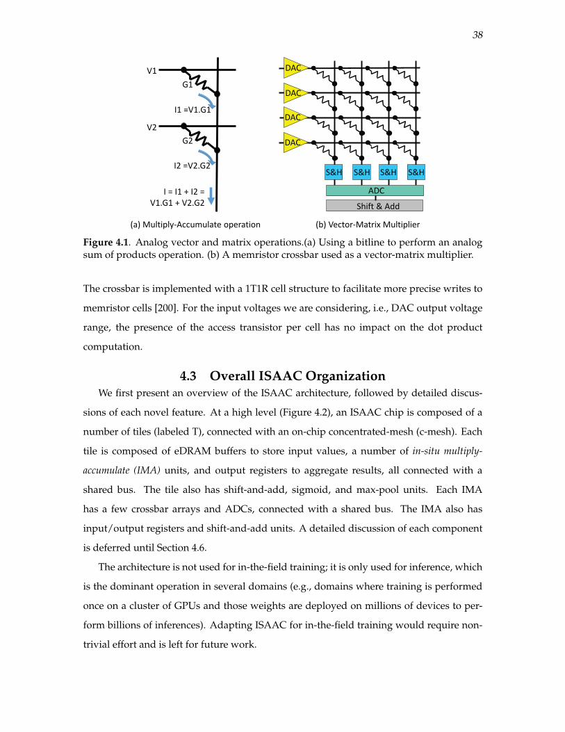
38
G1
I1 =V1.G1
V1
G2
I2 =V2.G2
V2
I = I1 + I2 =V1.G1 + V2.G2
(a) Multiply-Accumulate operation
DAC
S&H
ADC
Shift & Add
(b) Vector-Matrix Multiplier
S&H S&H S&H
DAC
DAC
DAC
Figure 4.1. Analog vector and matrix operations.(a) Using a bitline to perform an analogsum of products operation. (b) A memristor crossbar used as a vector-matrix multiplier.
The crossbar is implemented with a 1T1R cell structure to facilitate more precise writes to
memristor cells [200]. For the input voltages we are considering, i.e., DAC output voltage
range, the presence of the access transistor per cell has no impact on the dot product
computation.
4.3 Overall ISAAC OrganizationWe first present an overview of the ISAAC architecture, followed by detailed discus-
sions of each novel feature. At a high level (Figure 4.2), an ISAAC chip is composed of a
number of tiles (labeled T), connected with an on-chip concentrated-mesh (c-mesh). Each
tile is composed of eDRAM buffers to store input values, a number of in-situ multiply-
accumulate (IMA) units, and output registers to aggregate results, all connected with a
shared bus. The tile also has shift-and-add, sigmoid, and max-pool units. Each IMA
has a few crossbar arrays and ADCs, connected with a shared bus. The IMA also has
input/output registers and shift-and-add units. A detailed discussion of each component
is deferred until Section 4.6.
The architecture is not used for in-the-field training; it is only used for inference, which
is the dominant operation in several domains (e.g., domains where training is performed
once on a cluster of GPUs and those weights are deployed on millions of devices to per-
form billions of inferences). Adapting ISAAC for in-the-field training would require non-
trivial effort and is left for future work.
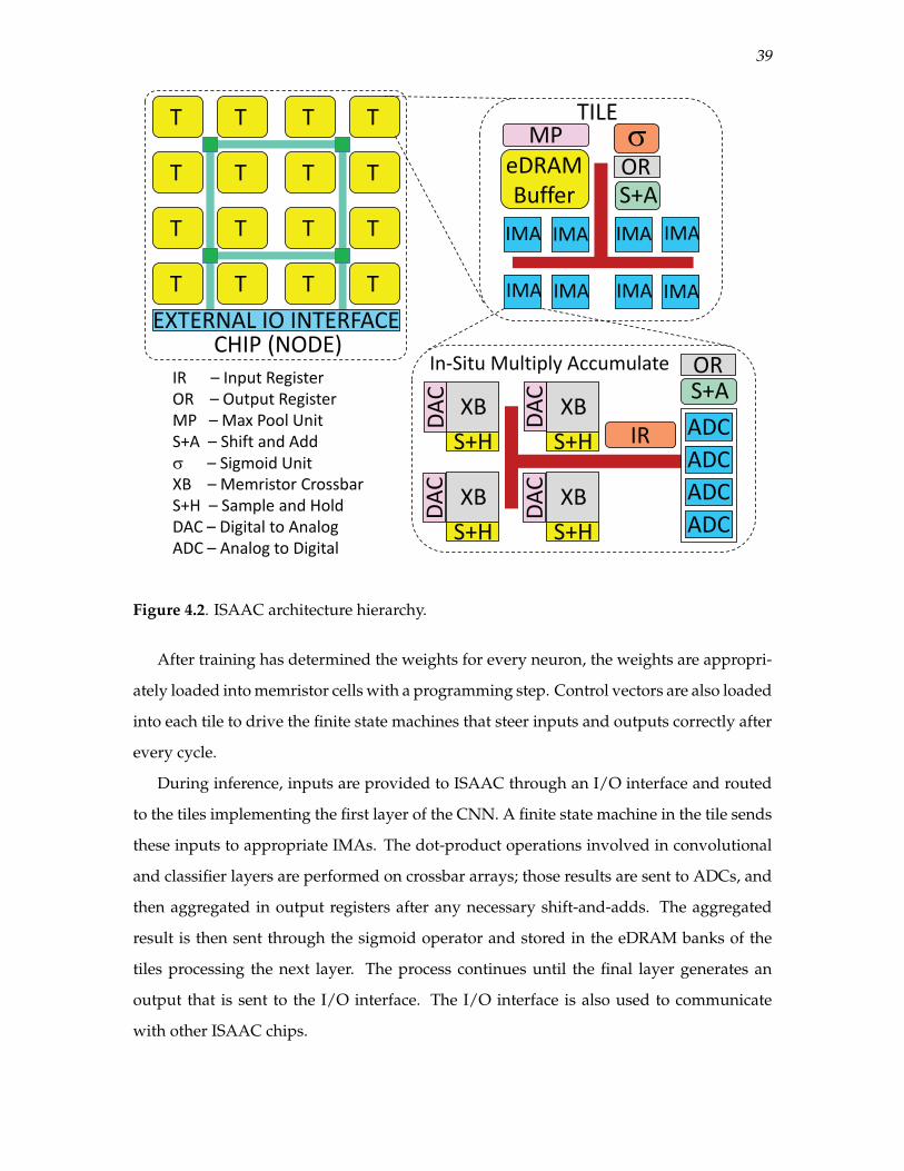
39
T T T T
T T T T
T T T T
T T T T
IMA
eDRAMBuffer
MP
S+A
S+A
TILE
DAC
S+HXB
S+HXB
S+HXB
S+HXB
ADCADCADCADC
In-Situ Multiply Accumulate
OR
EXTERNAL IO INTERFACE
DAC
DAC
DAC
IR
ORCHIP (NODE)
IR – Input RegisterOR – Output RegisterMP – Max Pool UnitS+A – Shift and Add
– Sigmoid UnitXB – Memristor CrossbarS+H – Sample and HoldDAC – Digital to AnalogADC – Analog to Digital
IMA IMA IMA
IMA IMA IMA IMA
Figure 4.2. ISAAC architecture hierarchy.
After training has determined the weights for every neuron, the weights are appropri-
ately loaded into memristor cells with a programming step. Control vectors are also loaded
into each tile to drive the finite state machines that steer inputs and outputs correctly after
every cycle.
During inference, inputs are provided to ISAAC through an I/O interface and routed
to the tiles implementing the first layer of the CNN. A finite state machine in the tile sends
these inputs to appropriate IMAs. The dot-product operations involved in convolutional
and classifier layers are performed on crossbar arrays; those results are sent to ADCs, and
then aggregated in output registers after any necessary shift-and-adds. The aggregated
result is then sent through the sigmoid operator and stored in the eDRAM banks of the
tiles processing the next layer. The process continues until the final layer generates an
output that is sent to the I/O interface. The I/O interface is also used to communicate
with other ISAAC chips.
40
At a high level, ISAAC implements a hierarchy of chips/tiles/IMAs/arrays and c-
mesh/bus. While the hierarchy is similar to that of DaDianNao, the internals of each tile
and IMA are very different. A hierarchical topology enables high internal bandwidth, re-
duced data movement when aggregating results, short bitlines and wordlines in crossbars,
and efficient resource partitioning across the many layers of a CNN.
4.4 The ISAAC PipelineDaDianNao operates on one CNN layer at a time. All the NFUs in the system are lever-
aged to perform the required operations for one layer in parallel. The synaptic weights for
that layer are therefore scattered across eDRAM banks in all tiles. The outputs are stored in
eDRAM banks and serve as inputs when the next layer begins its operation. DaDianNao
therefore maximizes throughput for one layer. This is possible because it is relatively easy
for an NFU to context-switch from operating on one layer to operating on a different layer
– it simply has to bring in a new set of weights from the eDRAM banks to its SRAM buffers.
On the other hand, ISAAC uses memristor arrays to not only store the synaptic weights,
but also perform computations on them. The in-situ computing approach requires that if
an array has been assigned to store weights for a CNN layer, it has also been assigned
to perform computations for that layer. Therefore, unlike DaDianNao, the tiles/IMAs of
ISAAC have to be partitioned across the different CNN layers. For example, tiles 0-3 may
be assigned to layer 0, tiles 4-11 may be assigned to layer 1, and so on. In this case, tiles
0-3 would store all weights for layer 0 and perform all layer 0 computations in parallel.
The outputs of layer 0 are sent to some of the tiles 4-11; once enough layer 0 outputs are
buffered, tiles 4-11 perform the necessary layer 1 computations, and so on.
To understand how results are passed from one stage to the next, consider the following
example, also shown in Figure 4.3. Assume that in layer i, a 6×6 input feature map is being
convolved with a 2×2 kernel to produce an output feature map of the same size. Assume
that a single column in an IMA has the four synaptic weights used by the 2×2 kernel. The
previous layer i − 1 produces outputs 0, 1, 2, ..., 6, 7, shown in blue in Figure 4.3a. All
of these values are placed in the input buffer for layer i. At this point, we have enough
information to start the operations for layer i. So inputs 0, 1, 6, 7 are fed to the IMA and
they produce the first output for layer i. When the previous layer i − 1 produces output

41
Figure 4.3. Minimum input buffer requirement for a 6× 6 input feature map with a 2× 2kernel and stride of 1. The blue values in (a), (b), and (c) represent the buffer contents foroutput neurons 0, 1, and 7, respectively.
8, it gets placed in the input buffer for layer i. Value 0, shown in green in Figure 4.3b, is
no longer required and can be removed from the input buffer. Thus, every new output
produced by layer i − 1 allows layer i to advance the kernel by one step and perform a
new operation of its own. Figure 4.3c shows the state of the input buffer a few steps later.
Note that a set of inputs is fed to No f convolutional kernels to produce No f output feature
maps. Each of these kernels constitutes a different column in a crossbar and operates on a
set of inputs in parallel.
We now discuss two important properties of this pipeline. The first pertains to buffer-
ing requirements in eDRAM between layers. The second pertains to synaptic weight
storage in memristors to design a balanced pipeline. In our discussions, a cycle is the time
required to perform one crossbar read operation, which for most of our analysis is 100 ns.
The eDRAM buffer requirement between two layers is fixed. In general terms, the size
of the buffer is:
((Nx × (Ky − 1)) + Kx)× Ni f
where Nx is the number of rows in the input feature map, Ky and Kx are the number of
columns and rows in the kernel, and Ni f is the number of input feature maps involved
in the convolution step. Without pipelining, the entire output (Nx × Ny × Ni f ) from layer

42
i − 1 would have to be stored before starting layer i. Thus, pipelining helps reduce the
buffering requirement by approximately Ny/Ky.
The Kx × Ky kernel is moved by strides Sx and Sy after every step. If say Sx = 2 and
Sy = 1, the previous layer i − 1 has to produce two values before layer i can perform its
next step. This can cause an unbalanced pipeline where the IMAs of layer i− 1 are busy in
every cycle, while the IMAs of layer i are busy in only every alternate cycle. To balance the
pipeline, we double the resources allocated to layer i− 1. In essence, the synaptic weights
for layer i− 1 are replicated in a different crossbar array so that two different input vectors
can be processed in parallel to produce two output values in one cycle. Thus, to estimate
the total synaptic storage requirement for a balanced pipeline, we work our way back from
the last layer. If the last layer is expected to produce outputs in every cycle, it will need
to store Kx × Ky × Ni f × No f synaptic weights. This term for layer i is referred to as Wi.
If layer i is producing a single output in a cycle, the storage requirement for layer i − 1
is Wi−1 × Sxi × Syi. Based on the values of Sx and Sy for each layer, the weights in early
layers may be replicated several times. If the aggregate storage requirement exceeds the
available storage on the chip by a factor of 2×, then the storage allocated to every layer
(except the last) is reduced by 2×. The pipeline remains balanced and most IMAs are busy
in every cycle, but the very last layer performs an operation and produces a result only in
every alternate cycle.
A natural question arises: is such a pipelined approach useful in DaDianNao as well?
If we can design a well-balanced pipeline and keep every NFU busy in every time step
in DaDianNao, to a first order, the pipelined approach will match the throughput of the
nonpipelined approach. The key here is that ISAAC needs pipelining to keep most IMAs
busy most of the time, whereas DaDianNao is able to keep most NFUs busy most of the
time without the need for pipelining.
4.5 Managing Bits, ADCs, and Signed Arithmetic4.5.1 The Read/ADC Pipeline
The ADCs and DACs in every tile can represent a significant overhead. To reduce ADC
overheads, we employ a few ADCs in one IMA, shared by multiple crossbars. We need
enough ADCs per IMA to match the read throughput of the crossbars. For example, a

43
128×128 crossbar may produce 128 bitline currents every 100 ns (one cycle, which is the
read latency for the crossbar array). To create a pipeline within the IMA, these bitline
currents are latched in 128 sample-and-hold circuits [141]. In the next 100 ns cycle, these
analog values in the sample-and-holds are fed sequentially to a single 1.28 giga-samples-
per-second (GSps) ADC unit. Meanwhile, in a pipelined fashion, the crossbar begins its
next read operation. Thus, 128 bitline currents are processed in 100 ns, before the next set
of bitline currents are latched in the sample-and-hold circuits.
4.5.2 Input Voltages and DACs
Each row in a crossbar array needs an input voltage produced by a DAC. We’ll assume
that every row receives its input voltage from a dedicated n-bit DAC. Note that a 1-bit
DAC is a trivial circuit (an inverter).
Next, we show how high precision and efficiency can be achieved, while limiting
the size of the ADC and DAC. We target 16-bit fixed-point arithmetic, partially because
prior work has shown that 16-bit arithmetic is sufficient for this class of machine learn-
ing algorithms [28], [67], and partially to perform an apples-to-apples comparison with
DaDianNao.
To perform a 16-bit multiplication in every memristor cell, we would need a 16-bit
DAC to provide the input voltage, 216 resistance levels in each cell, and an ADC capable
of handling well over 16 bits. It is clear that such a naive approach would have enormous
overheads and be highly error-prone.
To address this, we first mandate that the input be provided as multiple sequential bits.
Instead of a single voltage level that represents a 16-bit fixed-point number, we provide 16
voltage levels sequentially, where voltage level i is a 0/1 binary input representing bit i of
the 16-bit input number. The first cycle of this iterative process multiplies-and-adds bit 1
of the inputs with the synaptic weights, and stores the result in an output register (after
sending the sum of products through the ADC). The second cycle multiplies bit 2 of the
inputs with the synaptic weights, shifts the result one place to the left, and adds it to the
output register. The process continues until all 16 bits of the input have been handled in
16 cycles. This algorithm is similar to the classic multiplication algorithm used in modern
multiplier units. In this example where the input is converted into 1-bit binary voltage

44
levels, the IMA has to perform 16 sequential operations and we require a simple 1-bit
DAC. We could also accept a v-bit input voltage, which would require 16/v sequential
operations and a v-bit DAC. We later show that the optimal design point uses v = 1 and
eliminates the need for an explicit DAC circuit.
One way to reduce the sequential 16-cycle delay is to replicate the synaptic weights
on (say) two IMAs. Thus, one IMA can process the 8 most significant bits of the input,
while the other IMA can process the 8 least significant bits of the input. The results are
merged later after the appropriate shifting. This halves the latency for one 16-bit dot-
product operation while requiring twice as much storage budget. In essence, if half the
IMAs on a chip are not utilized, we can replicate all the weights and roughly double system
throughput.
4.5.3 Synaptic Weights and ADCs
Having addressed the input values and the DACs, we now turn our attention to the
synaptic weights and the ADCs. It is impractical to represent a 16-bit synaptic weight in a
single memristor cell. We therefore represent one 16-bit synaptic weight with 16/w w-bit
cells located in the same row. For the rest of this discussion, we assume w = 2 because
it emerges as a sweet spot in our design space exploration. When an input is provided,
the cells in a column perform their sum of products operations. The results of adjacent
columns must then be merged with the appropriate set of shifts and adds.
If the crossbar array has R rows, a single column is adding the results of R multipli-
cations of v-bit inputs and w-bit synaptic weights. The number of bits in the resulting
computation dictates the resolution A and size of the ADC. The relationship is as follows:
A = log(R) + v + w, i f v > 1 and w > 1 (4.1)
A = log(R) + v + w− 1, otherwise (4.2)
Thus, the design of ISAAC involves a number of independent parameters (v, w, R, etc.)
that impact overall throughput, power, and area in nontrivial ways.
4.5.4 Encoding to Reduce ADC Size
To further reduce the size of the ADC, we devise an encoding where every w-bit synap-
tic weight in a column is stored in its original form, or in its “flipped” form. The flipped
45
form of w-bit weight W is represented as W = 2w − 1−W. If the weights in a column
are collectively large, i.e., with maximal inputs, the sum-of-products yields an MSB of 1,
the weights are stored in their flipped form. This guarantees that the MSB of the sum-of-
products will be 0. By guaranteeing an MSB of 0, the ADC size requirement is lowered by
one bit.
The sum-of-products for a flipped column is converted to its actual value with the
following equation:R−1
∑i=0
ai × Wi =R−1
∑i=0
ai × (2w − 1−Wi) = (2w − 1)R−1
∑i=0
ai −R−1
∑i=0
ai ×Wi
where ai refers to the ith input value. The conversion requires us to compute the sum of the
current input values ai, which is done with one additional column per array, referred to as
the unit column. During an IMA operation, the unit column produces the result ∑R−1i=0 ai.
The results of any columns that have been stored in flipped form is subtracted from the
results of the unit column. In addition, we need a bit per column to track if the column has
original or flipped weights.
The encoding scheme can be leveraged either to reduce ADC resolution, increase cell
density, or increase the rows per crossbar. At first glance, it may appear that a 1-bit
reduction in ADC resolution is not a big deal. As we show later, because ADC power
is a significant contributor to ISAAC power, and because some ADC overheads grow
exponentially with resolution, the impact of this technique on overall ISAAC efficiency
is very significant. In terms of overheads, the columns per array have grown from 128 to
129 and one additional shift-and-add has been introduced. Note that the shift-and-add
circuits represent a small fraction of overall chip area and there is more than enough time
in one cycle (100 ns) to perform a handful of shift-and-adds and update the output register.
Our analysis considers these overheads.
4.5.5 Correctly Handling Signed Arithmetic
Synaptic weights in machine learning algorithms can be positive or negative. It is
important to allow negative weights so the network can capture inhibitory effects of fea-
tures [178]. We must therefore define bit representations that perform correct signed arith-
metic operations, given that a memristor bitline can only add currents. There are a number
of ways that signed numbers can be represented and we isolate the best approach below.

46
This approach is also compatible with the encoding previously described. In fact, it lever-
ages the unit column introduced earlier.
We assume that inputs to the crossbar arrays are provided with a 2’s complement
representation. For a 16-bit signed fixed-point input, a 1 in the ith bit represents a quantity
of 2i (0 ≤ i < 15) or −2i (i = 15). Since we have already decided to provide the input one
bit at a time, this is easily handled – the result of the last dot-product operation undergoes
a shift-and-subtract instead of a shift-and-add.
Similarly, we could have considered a 2’s complement representation for the synaptic
weights in the crossbars too, and multiplied the quantity produced by the most significant
bit by −215. But because each memristor cell stores two bits, it is difficult to isolate the
contribution of the most significant bit. Therefore, for synaptic weights, we use a repre-
sentation with a bias (similar to the exponent in the IEEE 754 floating-point standard). A
16-bit fixed-point weight between −215 and 215 − 1 is represented by an unsigned 16-bit
integer, and the conversion is performed by subtracting a bias of 215. Since the bitline
output represents a sum of products with biased weights, the conversion back to a signed
fixed-point value will require that the biases be subtracted, and we need to subtract as
many biases as the 1s in the input. Thankfully, the unit column has already counted the
number of 1s in the input. This count is multiplied by the bias of 215 and subtracted from
the end result. The subtraction due to encoding scheme and the subtraction due to bias
combines to a single subtraction from the end result.
In summary, this section has defined bit representations for the input values and the
synaptic weights so that correct signed arithmetic can be performed, and the overheads of
ADCs and DACs are kept in check. The proposed approach incurs additional shift-and-
add operations (a minor overhead), 16-iteration IMA operations to process a 16-bit input,
and 8 cells per synaptic weight. Our design space exploration shows that these choices
best balance the trade-offs.
4.6 Example and Intra-Tile PipelineAnalog units can be ideal for specific functions. But to execute a full-fledged CNN/DNN,
the flow of data has to be orchestrated with a number of digital components. This section
describes the operations of these supporting digital components and how these operations

47
are pipelined.
This is best explained with the example shown in Figure 4.4. In this example, layer i
is performing a convolution with a 4× 4 shared kernel. The layer receives 16 input filters
and produces 32 output filters (see Figure 4.4a). These output filters are fed to layer i + 1
that performs a max-pool operation on every 2× 2 grid. The 32 down-sized filters are then
fed as input to layer i + 2. For this example, assume that kernel strides (Sx and Sy) are
always 1. We assume that one IMA has four crossbar arrays, each with 128 rows and 128
columns.
Layer i performs a dot-product operation with a 4× 4× 16 matrix, i.e., we need 256
multiply-add operations, or a crossbar with 256 rows. Since there are 32 output filters,
32 such operations are performed in parallel. Because each of these 32 operations is per-
formed across 8 2-bit memristor cells in a row, we need a crossbar with 256 columns. Since
the operation requires a logical crossbar array of size 256× 256, it must be spread across
4 physical crossbar arrays of size 128× 128. A single IMA may be enough to perform the
computations required by layer i.
The outputs of layer i− 1 are stored in the eDRAM buffer for layer i’s tile. As described
in Figure 4.3, when a new set of inputs (Ni 16-bit values) shows up, it allows layer i to
proceed with its next operation. This operation is itself pipelined (shown in detail in
Figure 4.4b), with the cycle time (100 ns) dictated by the slowest stage, which is the crossbar
read. In the first cycle, an eDRAM read is performed to read out 256 16-bit inputs. These
values are sent over the shared bus to the IMA for layer i and recorded in the input register
(IR). The IR has a maximum capacity of 1KB and is implemented with SRAM. The entire
copy of up to 1KB of data from eDRAM to IR is performed within a 100 ns stage. We design
our eDRAM and shared bus to support this maximum bandwidth.
Once the input values have been copied to the IR, the IMA will be busy with the dot-
product operation for the next 16+ cycles. In the next 16 cycles, the eDRAM is ready
to receive other inputs and deal with other IMAs in the tile, i.e., it context-switches to
handling other layers that might be sharing that tile while waiting for the result of one
IMA.
Over the next 16 cycles, the IR feeds 1 bit at a time for each of the 256 input values to
the crossbar arrays. The first 128 bits are sent to crossbars 0 and 1, and the next 128 bits

48
16 Input filters for Layer i
Layer i: convolution with a 4x4x16 matrix to
produce an output filter
32 Output filters
Layer i+1: maxpool(2,2)
32 Output filters
Inputs to Layer i+2
Cyc 1 2 3 4 … 17 18 19 20 21 22eDRAMRd + IR
Xbar1
Xbar2
Xbar3
Xbar16 ADC S+A
OR wrS+A
OR wreDRAM
Wr…
Tile IMA IMA IMA IMA IMA IMA Tile Tile Tile
(a) Example CNN with
layers i, i+1, i+2
(b) Example of one operation in layer i flowing through its pipeline
Figure 4.4. Example CNN layer traversing the ISAAC pipeline.
are sent to crossbars 2 and 3. At the end of each 100 ns cycle, the outputs are latched in
the Sample & Hold circuits. In the next cycle, these outputs are fed to the ADC units. The
results of the ADCs are then fed to the shift-and-add units, where the results are merged
with the output register (OR) in the IMA.
The OR is a 128B SRAM structure. In this example, it produces 32 16-bit values over a
16-cycle period. In each cycle, the results of the ADCs are shifted and added to the value
in the OR (this includes the shift-and-adds required by the encoding schemes). Since we
have 100 ns to update up to 64 16-bit values, we only need 4 parallel shift-and-add units,
which represents a very small area overhead.
As shown in Figure 4.4b, at the end of cycle 19, the OR in the IMA has its final output
value. This is sent over the shared bus to the central units in the tile. These values may
undergo another step of shift-and-adds and merging with the central OR in the tile if the
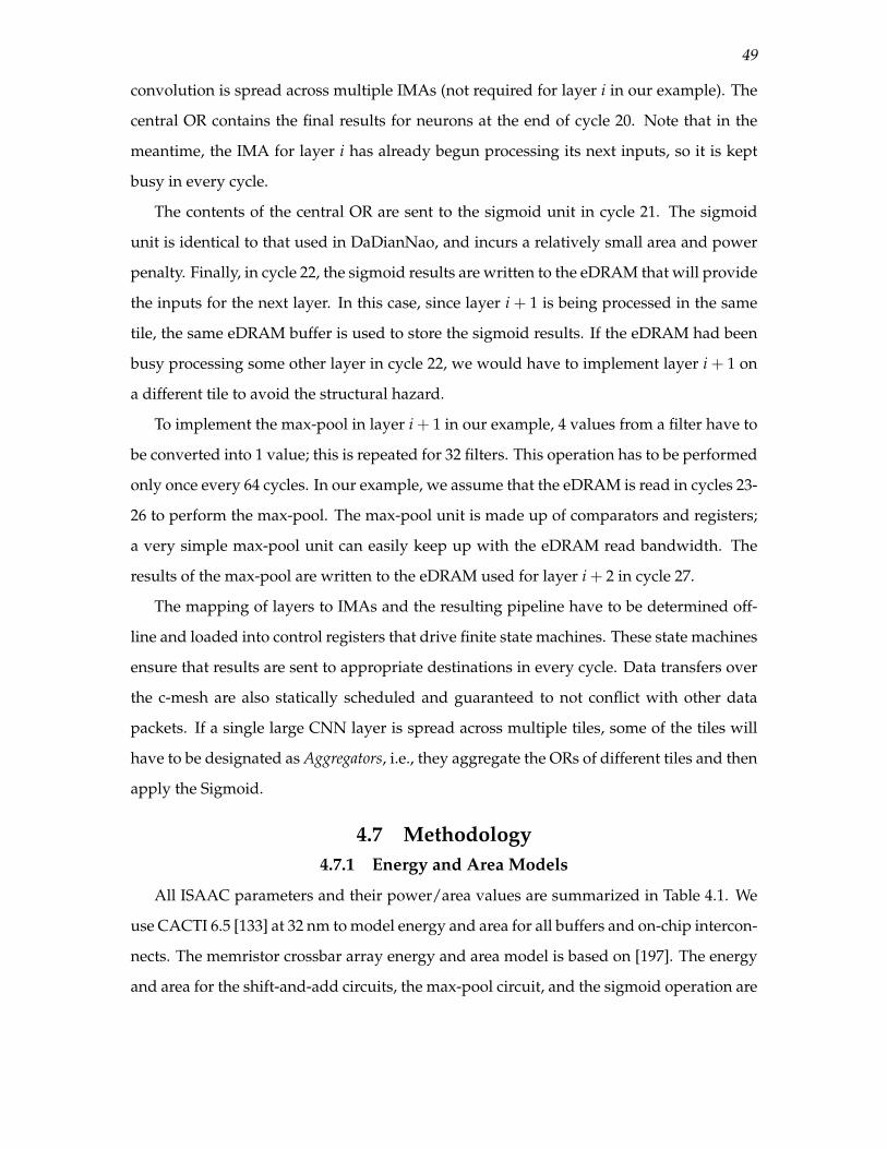
49
convolution is spread across multiple IMAs (not required for layer i in our example). The
central OR contains the final results for neurons at the end of cycle 20. Note that in the
meantime, the IMA for layer i has already begun processing its next inputs, so it is kept
busy in every cycle.
The contents of the central OR are sent to the sigmoid unit in cycle 21. The sigmoid
unit is identical to that used in DaDianNao, and incurs a relatively small area and power
penalty. Finally, in cycle 22, the sigmoid results are written to the eDRAM that will provide
the inputs for the next layer. In this case, since layer i + 1 is being processed in the same
tile, the same eDRAM buffer is used to store the sigmoid results. If the eDRAM had been
busy processing some other layer in cycle 22, we would have to implement layer i + 1 on
a different tile to avoid the structural hazard.
To implement the max-pool in layer i + 1 in our example, 4 values from a filter have to
be converted into 1 value; this is repeated for 32 filters. This operation has to be performed
only once every 64 cycles. In our example, we assume that the eDRAM is read in cycles 23-
26 to perform the max-pool. The max-pool unit is made up of comparators and registers;
a very simple max-pool unit can easily keep up with the eDRAM read bandwidth. The
results of the max-pool are written to the eDRAM used for layer i + 2 in cycle 27.
The mapping of layers to IMAs and the resulting pipeline have to be determined off-
line and loaded into control registers that drive finite state machines. These state machines
ensure that results are sent to appropriate destinations in every cycle. Data transfers over
the c-mesh are also statically scheduled and guaranteed to not conflict with other data
packets. If a single large CNN layer is spread across multiple tiles, some of the tiles will
have to be designated as Aggregators, i.e., they aggregate the ORs of different tiles and then
apply the Sigmoid.
4.7 Methodology4.7.1 Energy and Area Models
All ISAAC parameters and their power/area values are summarized in Table 4.1. We
use CACTI 6.5 [133] at 32 nm to model energy and area for all buffers and on-chip intercon-
nects. The memristor crossbar array energy and area model is based on [197]. The energy
and area for the shift-and-add circuits, the max-pool circuit, and the sigmoid operation are

50
Table 4.1. ISAAC Parameters.
ISAAC Tile at 1.2 GHz, 0.37 mm2
Component Params Spec Power Area (mm2)eDRAM size 64KB 20.7 mW 0.083Buffer num banks 4
bus width 256 beDRAM num wire 384 7 mW 0.090
-to-IMA busRouter flit size 32 42 mW 0.151
num port 8 (shared by4 tiles)
Sigmoid number 2 0.52 mW 0.0006S+A number 1 0.05 mW 0.00006
MaxPool number 1 0.4 mW 0.00024OR size 3 KB 1.68 mW 0.0032
Total 40.9 mW 0.215 mm2
IMA properties (12 IMAs per tile)ADC resolution 8 bits 16 mW 0.0096
frequency 1.2 GSpsnumber 8
DAC resolution 1 bit 4 mW 0.00017number 8× 128
S+H number 8× 128 10 uW 0.00004Memristor number 8 2.4 mW 0.0002
array size 128× 128bits per cell 2
S+A number 4 0.2 mW 0.00024IR size 2 KB 1.24 mW 0.0021OR size 256 B 0.23 mW 0.00077
IMA Total number 12 289 mW 0.157 mm2
1 Tile Total 330 mW 0.372 mm2
168 Tile Total 55.4 W 62.5 mm2
Hyper Tr links/freq 4/1.6GHz 10.4 W 22.88link bw 6.4 GB/s
Chip Total 65.8 W 85.4 mm2
DaDianNao at 606 MHz scaled up to 32nmeDRAM size 36 MB 4.8 W 33.22
num banks 4 per tileNFU number 16 4.9 W 16.22
Global Bus width 128 bit 13 mW 15.716 Tile Total 9.7 W 65.1 mm2
Hyper Tr links/freq 4/1.6GHz 10.4 W 22.88link bw 6.4 GB/s
Chip Total 20.1 W 88 mm2

51
adapted from the analysis in DaDianNao [32].
For off-chip links, we employ the same HyperTransport serial link model as that used
by DaDianNao [32]. For ADC energy and area, we use data from a recent survey [134] of
ADC circuits published at major circuit conferences. For most of our analysis, we use
an 8-bit ADC at 32 nm that is optimized for area. We also considered ADCs that are
optimized for power, but the high area and low sampling rates of these designs made them
impractical (450 KHz in 0.12 mm2 [98]). An SAR ADC has four major components [98]: a
vref buffer, memory, clock, and a capacitive DAC. To arrive at power and area for the same
style ADC, but with different bit resolutions, we scaled the power/area of the vref buffer,
memory, and clock linearly, and the power/area of the capacitive DAC exponentially [158].
For most of the chapter, we assume a simple 1-bit DAC because we need a DAC for
every row in every memristor array. To explore the design space with multibit DACs, we
use the power/area model in [158].
The energy and area estimates for DaDianNao are taken directly from that work [32],
but scaled from 28 nm to 32 nm for an apples-to-apples comparison. Also, we assume
a similar sized chip for both (an iso-area comparison) – our analysis in Table 4.1 shows
that one ISAAC chip can accommodate 14×12 tiles. It is worth pointing out that DaDi-
anNao’s eDRAM model, based on state-of-the-art eDRAMs, yields higher area efficiency
than CACTI’s eDRAM model.
4.7.2 Performance Model
We have manually mapped each of our benchmark applications to the IMAs, tiles,
and nodes in ISAAC. Similar to the example discussed in Section 4.6, we have made
sure that the resulting pipeline between layers and within a layer does not have any
structural hazards. Similarly, data exchange between tiles on the on-chip and off-chip
network has also been statically routed without any conflicts. This gives us a deterministic
execution model for ISAAC and the latency/throughput for a given CNN/DNN can be
expressed with analytical equations. The performance for DaDianNao can also be similarly
obtained. Note that CNNs/DNNs executing on these tiled accelerators do not exhibit any
run-time dependences or control-flow, i.e., cycle-accurate simulations do not capture any
phenomena not already captured by our analytical estimates.

52
4.7.3 Metrics
We consider three key metrics:
1. CE: Computational Efficiency is represented by the number of 16-bit operations per-
formed per second per mm2 (GOPS/s×mm2).
2. PE: Power Efficiency is represented by the number of 16-bit operations performed
per watt (GOPS/W).
3. SE: Storage Efficiency is the on-chip capacity for synaptic weights per unit area
(MB/mm2).
We first compute the peak capabilities of the architectures for each of these metrics.
We then compute these metrics for our benchmark CNNs/DNNs – based on how the
CNN/DNN maps to the tiles/IMAs, some IMAs may be under-utilized.
4.7.4 Benchmarks
Based on the discussion in Section 4.2.2, we use seven benchmark CNNs and two
DNNs. Four of the CNNs are versions of the Oxford VGG [168], and three are versions
of MSRA [73] – both are architectures proposed in ILSVRC 2014. DeepFace is a complete
DNN [194] while the last workload is a large DNN layer [100] also used in the DaDianNao
paper [32]. Table 4.2 lists the parameters for these CNNs and DNNs. The largest workload
has 26 layers and 330 million parameters.
4.8 Results4.8.1 Analyzing ISAAC
4.8.1.1 Design Space Exploration
ISAAC’s behavior is a function of many parameters: (1) the size of the memristor
crossbar array, (2) the number of crossbars in an IMA, (3) the number of ADCs in an IMA,
and (4) the number of IMAs in a tile. The size of the central eDRAM buffer in a node is
set to 64 KB and the c-mesh flit width is set to 32 bits. These were set to limit the search
space and were determined based on the buffering/communication requirements for the
largest layers in our benchmarks. Many of the other parameters, e.g., the resolution of the
ADC, and the width of the bus connecting the eDRAM and the IMAs, are derived from the
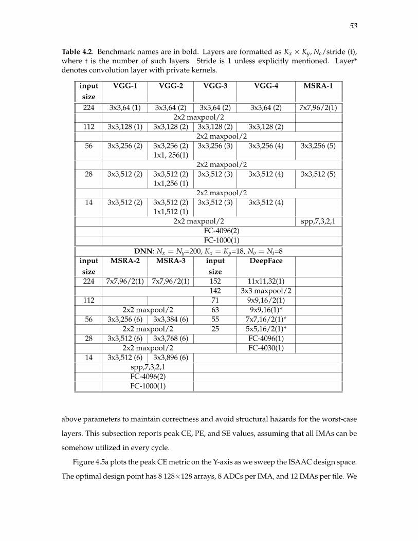
53
Table 4.2. Benchmark names are in bold. Layers are formatted as Kx × Ky, No/stride (t),where t is the number of such layers. Stride is 1 unless explicitly mentioned. Layer*denotes convolution layer with private kernels.
input VGG-1 VGG-2 VGG-3 VGG-4 MSRA-1size224 3x3,64 (1) 3x3,64 (2) 3x3,64 (2) 3x3,64 (2) 7x7,96/2(1)
2x2 maxpool/2112 3x3,128 (1) 3x3,128 (2) 3x3,128 (2) 3x3,128 (2)
2x2 maxpool/256 3x3,256 (2) 3x3,256 (2) 3x3,256 (3) 3x3,256 (4) 3x3,256 (5)
1x1, 256(1)2x2 maxpool/2
28 3x3,512 (2) 3x3,512 (2) 3x3,512 (3) 3x3,512 (4) 3x3,512 (5)1x1,256 (1)
2x2 maxpool/214 3x3,512 (2) 3x3,512 (2) 3x3,512 (3) 3x3,512 (4)
1x1,512 (1)2x2 maxpool/2 spp,7,3,2,1
FC-4096(2)FC-1000(1)
DNN: Nx = Ny=200, Kx = Ky=18, No = Ni=8input MSRA-2 MSRA-3 input DeepFacesize size224 7x7,96/2(1) 7x7,96/2(1) 152 11x11,32(1)
142 3x3 maxpool/2112 71 9x9,16/2(1)
2x2 maxpool/2 63 9x9,16(1)*56 3x3,256 (6) 3x3,384 (6) 55 7x7,16/2(1)*
2x2 maxpool/2 25 5x5,16/2(1)*28 3x3,512 (6) 3x3,768 (6) FC-4096(1)
2x2 maxpool/2 FC-4030(1)14 3x3,512 (6) 3x3,896 (6)
spp,7,3,2,1FC-4096(2)FC-1000(1)
above parameters to maintain correctness and avoid structural hazards for the worst-case
layers. This subsection reports peak CE, PE, and SE values, assuming that all IMAs can be
somehow utilized in every cycle.
Figure 4.5a plots the peak CE metric on the Y-axis as we sweep the ISAAC design space.
The optimal design point has 8 128×128 arrays, 8 ADCs per IMA, and 12 IMAs per tile. We
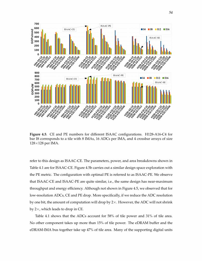
54
Figure 4.5. CE and PE numbers for different ISAAC configurations. H128-A16-C4 forbar I8 corresponds to a tile with 8 IMAs, 16 ADCs per IMA, and 4 crossbar arrays of size128×128 per IMA.
refer to this design as ISAAC-CE. The parameters, power, and area breakdowns shown in
Table 4.1 are for ISAAC-CE. Figure 4.5b carries out a similar design space exploration with
the PE metric. The configuration with optimal PE is referred to as ISAAC-PE. We observe
that ISAAC-CE and ISAAC-PE are quite similar, i.e., the same design has near-maximum
throughput and energy efficiency. Although not shown in Figure 4.5, we observed that for
low-resolution ADCs, CE and PE drop. More specifically, if we reduce the ADC resolution
by one bit, the amount of computation will drop by 2×. However, the ADC will not shrink
by 2×, which leads to drop in CE.
Table 4.1 shows that the ADCs account for 58% of tile power and 31% of tile area.
No other component takes up more than 15% of tile power. The eDRAM buffer and the
eDRAM-IMA bus together take up 47% of tile area. Many of the supporting digital units

55
(shift-and-add, MaxPool, Sigmoid, SRAM buffers) take up negligibly small amounts of
area and power.
For space reasons, we don’t show the design space for the SE metric, but identify
ISAAC-SE in Figure 4.5. We note that ISAAC-CE, ISAAC-PE, and ISAAC-SE have SE
values of 0.96 MB/mm2, 1 MB/mm2, and 54.79 MB/mm2, respectively. It is worth not-
ing that while ISAAC-SE cannot achieve the performance and energy of ISAAC-CE and
ISSAC-PE, it can implement a large network with fewer chips. For example, the large DNN
benchmark can fit in just one ISAAC-SE chip, while it needs 32 ISAAC-CE chips, and 64
DaDianNao chips. This makes ISAAC-SE an attractive design point when constrained by
cost or board layouts.
As a sensitivity, we also consider the impact of moving to 32-bit fixed point computa-
tions, while keeping the same bus bandwidth. This would reduce overall throughput by
4× since latency per computation and storage requirements are both doubled. Similarly, if
crossbar latency is assumed to be 200 ns, throughput is reduced by 2×, but because many
of the structures become simpler, CE is only reduced by 30%.
4.8.2 Impact of Pipelining
ISAAC’s pipeline enables a reduction in the buffering requirements between consec-
utive layers and an increase in throughput. The only downside is an increase in power
because pipelining allows all layers to be simultaneously busy.
Table 4.3 shows the input buffering requirements for the biggest layers in our bench-
Table 4.3. Buffering requirement with and without pipelining for the largest layers.
Ni, k ,Nx No pipeline (KB) With pipeline (KB)VGG and MSRA
3,3,224 147 1.9696,7,112 1176 7464,3,112 784 21128,3,56 392 21256,3,28 196 21384,3,28 294 32512,3,14 98 21768,3,14 150 32
Deep Face142,11,32 142 48
71,3,32 71 6.563,9,16 15.75 8.855,9,16 13.57 7.725,7,16 6.25 2.7
56
marks with and without pipelining. In an ISAAC design without pipelining, we assume
a central buffer that stores the outputs of the currently executing layer. The size of this
central buffer is the maximum buffer requirement for any layer in Table 4.3, viz, 1,176 KB.
With the ISAAC pipeline, the buffers are scattered across the tiles. For our benchmarks, we
observe that no layer requires more than 74 KB of input buffer capacity. The layers with
the largest input buffers also require multiple tiles to store their synaptic weights. We are
therefore able to establish 64 KB as the maximum required size for the eDRAM buffer in a
tile. This small eDRAM size is an important contributor to the high CE and SE achieved
by ISAAC. Similarly, based on our benchmark behaviors, we estimate that the inter-tile
link bandwidth requirement never exceeds 3.2 GB/s. We therefore conservatively assume
a 32-bit link operating at 1 GHz.
The throughput advantage and power overhead of pipelining is a direct function of the
number of layers in the benchmark. For example, VGG-1 has 16 layers and the pipelined
version is able to achieve a throughput improvement of 16× over an unpipelined version
of ISAAC. The power consumption within the tiles also increases roughly 16× in VGG-1,
although system power does not increase as much because of the constant power required
by the HyperTransport links.
4.8.3 Impact of Data Layout and ADCs/DACs
As the power breakdown in Table 4.1 shows, the 96 ADCs in a tile account for 58% of
tile power. Recall that we had carefully mapped data to the memristor arrays to reduce
these overheads – we now quantitatively justify those choices.
In our analysis, we first confirmed that a 9-bit ADC is never worth the power/area
overhead. Once we limit ourselves to using an 8-bit ADC, a change to the DAC resolution
or the bits per cell is constrained by Equations 4.1 and 4.2. If one of these (v or w) is
increased linearly, the number of rows per array R must be reduced exponentially. This
reduces throughput per array. But it also reduces the eDRAM/bus overhead because the
IMA has to be fed with fewer inputs. We empirically estimated that the CE metric is maxi-
mized when using 2 bits per cell (w = 2). Performing a similar analysis for DAC resolution
v yields maximal CE for 1-bit DACs. Even though v and w have a symmetric impact
on R and eDRAM/bus overheads, the additional overhead of multibit DACs pushes the

57
balance further in favor of using a small value for v. In particular, using a 2-bit DAC
increases the area and power of a chip by 63% and 7%, respectively, without impacting
overall throughput. Similarly, going from a 2-bit cell to a 4-bit cell reduces CE and PE by
23% and 19%, respectively.
The encoding scheme introduced in Section 4.5 allows the use of a lower resolution
8-bit ADC. Without the encoding scheme, we would either need a 9-bit ADC or half as
many rows per crossbar array. The net impact is that the encoding scheme enables a 50%
and 87% improvement in CE and PE, respectively. Because of the nature of Equation 4.2,
a linear change to ADC resolution has an exponential impact on throughput; therefore,
saving a single bit in our computations is very important.
4.8.4 Comparison to DaDianNao
Table 4.4 compares peak CE, PE, and SE values for DaDianNao and ISAAC. DaDian-
Nao’s NFU unit has high computational efficiency – 344 GOPS/s×mm2. Adding eDRAM
banks, central I/O buffers, and interconnects brings CE down to 63.5 GOPS/s×mm2. On
the other hand, a 128×128 memristor array with 2 bits per cell has a CE of 1707 GOPS/s×
mm2. In essence, the crossbar is a very efficient way to perform a bulk of the neces-
sary bit arithmetic (e.g., adding 128 sets of 128 2-bit numbers) in parallel, with a few
shift-and-add circuits forming the tail end of the necessary arithmetic (e.g., merging 8
numbers). Adding ADCs, other tile overheads, and the eDRAM buffer brings the CE down
to 479 GOPS/s×mm2. The key to ISAAC’s superiority in CE is the fact that the memristor
array has very high computational parallelism, and storage density. Also, to perform any
computation, DaDianNao fetches two values from eDRAM, while ISAAC has to only fetch
one input from eDRAM (thanks to in-situ computing).
An ISAAC chip consumes more power (65.8 W) than a DaDianNao chip (20.1 W) of
the same size, primarily because it has higher computational density and because of ADC
overheads. In terms of PE though, ISAAC is able to beat DaDianNao by 27%. This is
partially because DaDianNao pays a higher “tax” on HyperTransport power than ISAAC.
The HT is a constant overhead of 10 W, representing half of DaDianNao chip power, but
only 16% of ISAAC chip power.
Next, we execute our benchmarks on ISAAC-CE and DaDianNao, while assuming 8-,

58
Table 4.4. Comparison of ISAAC and DaDianNao in terms of CE, PE, and SE. HyperTrans-port overhead is included.
Architecture CE PE SEGOPs/(s×mm2) GOPs/W MB/mm2
DaDianNao 63.46 286.4 0.41ISAAC-CE 478.95 363.7 0.74ISAAC-PE 466.8 380.7 0.71ISAAC-SE 140.3 255.3 54.8
16-, 32-, and 64-chip boards.
Figure 4.6a shows throughputs for our benchmarks for each case. We don’t show
results for the cases where DaDianNao chips do not have enough eDRAM storage to
accommodate all synaptic weights. In all cases, the computation spreads itself across
all available IMAs (ISAAC) or NFUs (DaDianNao) to maximize throughput. Figure 4.6b
performs a similar comparison in terms of energy.
For large benchmarks on many-chip configurations, DaDianNao suffers from the all-to-
all communication bottleneck during the last classifier layers. As a result, it has low NFU
utilization in these layers. Meanwhile, ISAAC has to replicate the weights in early layers
several times to construct a balanced pipeline. In fact, in some benchmarks, the first layer
has to be replicated more than 50K times to keep the last layer busy in every cycle. Since we
don’t have enough storage for such high degrees of replication, the last classifier layers also
see relatively low utilization in the IMAs. Thus, on early layers, ISAAC has a far higher
CE than early layers of DaDianNao – the actual speedups vary depending on the degree
of replication for each layer. In later layers, both operate at low utilization – DaDianNao
because of bandwidth limitations and ISAAC because of limitations on replication. The
net effect of these phenomena is that on average for 16-chip configurations, ISAAC-CE
achieves 14.8× higher throughput, consumes 95% more power, and achieves 5.5× lower
energy than DaDianNao.
While we don’t compare against state-of-the-art GPU implementations of CNNs, we
note that a 64-chip DaDianNao [32] has already been shown to have 450× speedup and
150× lower energy than an NVIDIA K20M GPU.
4.9 ConclusionsWhile the potential for crossbars as analog dot product engines is well known, our
work has shown that a number of challenges must be overcome to realize a full-fledged

59
Figure 4.6. Normalized throughput (top) and normalized energy (bottom) of ISAAC withrespect to DaDianNao.
CNN architecture. In particular, a balanced interlayer pipeline with replication, an intra-
tile pipeline, efficient handling of signed arithmetic, and bit encoding schemes are required
to deliver high throughput and manage the high overheads of ADCs, DACs, and eDRAMs.
We note that relative to DaDianNao, ISAAC is able to deliver higher peak computational
and power efficiency because of the nature of the crossbar, and in spite of the ADCs
accounting for nearly half the chip power. On benchmark CNNs and DNNs, we observe
that ISAAC is able to out-perform DaDianNao significantly in early layers, while the
last layers suffer from under-utilization in both architectures. On average for a 16-chip
configuration, ISAAC is able to yield a 14.8× higher throughput than DaDianNao.

CHAPTER 5
NEWTON: GRAVITATING TOWARDS THE
PHYSICAL LIMITS OF CROSSBAR
ACCELERATION
5.1 IntroductionAccelerators are in vogue today, primarily because it is evident that annual perfor-
mance improvements can be sustained via specialization. There are also many emerging
applications that demand high-throughput low-energy hardware, such as the machine
learning tasks that are becoming commonplace in enterprise servers, self-driving cars, and
mobile devices. The last two years have seen a flurry of activity in designing machine
learning accelerators [28], [32], [34], [51], [86], [112], [152], [165], [199]. Similar to our
work, most of these recent works have focused on inference in artificial neural networks,
and specifically deep convolutional networks, that achieve state-of-the-art accuracies on
challenging image classification workloads.
While most of these recent accelerators have used digital architectures [28], [32], a
few have leveraged analog acceleration on memristor crossbars [22], [34], [163]. Such
accelerators take advantage of in-situ computation to dramatically reduce data movement
costs. Each crossbar is assigned to execute parts of the neural network computation and
programmed with the corresponding weight values. Input neuron values are fed to the
crossbar, and by leveraging Kirchoff’s Law, the crossbar outputs the corresponding dot
product. The neuron output undergoes analog-to-digital conversion (ADC) before being
sent to the next layer. Multiple small-scale prototypes of this approach have also been
demonstrated [3], [125].
In this chapter, we focus on innovations to the recent ISAAC architecture [163]. While
ISAAC was able to provide an order of magnitude improvement in throughput, relative
to state-of-the-art digital architectures, it has a higher power density. This is primarily

61
because of the power and area overheads of ADC units. Therefore, we try to improve
various aspects of the ISAAC design, with a special emphasis on reducing ADC and other
resource requirements.
We introduce six innovations at different levels of the tile hierarchy. These innovations
leverage heterogeneous requirements of different parts of the neural network computa-
tion. They avoid over-provisioning ADC, HTree, and buffer resources. And finally, they
leverage numeric algorithms to further reduce the involvement of ADCs.
The new design, Newton, is moving the crossbar architecture closer to the bare min-
imum energy required to process one neuron. It does this by reducing the overheads
imposed by the architecture and by modern large workloads. We define our ideal neuron
as one that keeps the weight in-place adjacent to a digital ALU, retrieves the input from
an adjacent single-row eDRAM unit, and after performing one digital operation, writes
the result to another adjacent single-row eDRAM unit. This energy is lower than that for
a similarly ideal analog neuron because of the ADC cost. This ideal neuron operation
consumes 0.33 pJ. An average DaDianNao operation consumes 3.5 pJ because it pays
a high price in data movement for inputs and weights. An average ISAAC operation
consumes 1.8 pJ because it pays a moderate price in data movement for inputs (weights
are in-situ) and a high price for ADC. An average Eyeriss [31] operation consumes 1.67 pJ
because of an improved dataflow to maximize reuse. The innovations in Newton push the
analog architecture closer to the ideal neuron by consuming 0.85 pJ per operation. Relative
to ISAAC, Newton achieves a 77% decrease in power, 51% decrease in energy, and 2.2×
increase in throughput/area.
5.2 Background5.2.1 Workloads
We consider different CNNs presented in the ILSVRC challenge of image classification
for the IMAGENET [157] dataset. The suite of benchmarks considered in this chapter is
representative of the various dataflows in such image classification networks. For exam-
ple, Alexnet is the simplest of CNNs with a reasonable accuracy, where a few convolution
layers at the start extract features from the image, followed by fully connected layers that
classify the image. The other networks were designed with a similar structure but were

62
made deeper and wider with more parameters. For example, MSRA Prelu-net [73] has 14
more layers than Alexnet [96] and has 330 million parameters, which is 5.5× higher than
Alexnet. On the other hand, residual nets have forward connections with hops, i.e., output
of a layer is passed on to not only the next layer but subsequent layers. Even though the
number of parameters in Resnets [72] are much lower, these networks are much deeper
and have a different dataflow, which changes the buffering requirements in accelerator
pipelines.
5.2.2 The Landscape of CNN Accelerators
5.2.2.1 Digital Accelerators
The DianNao [28] and DaDianNao [32] accelerators were among the first to target deep
convolutional networks at scale. DianNao designs the digital circuits for a basic NFU
(Neural Functional Unit). DaDianNao is a tiled architecture where each tile has an NFU
and eDRAM banks that feed synaptic weights to that NFU. DaDianNao uses many tiles
on many chips to parallelize the processing of a single network layer. Once that layer
is processed, all the tiles then move on to processing the next layer in parallel. Recent
papers, e.g., Cnvlutin [5], have modified DaDianNao so the NFU does not waste time and
energy processing zero-valued inputs. EIE [165] and Minerva [152] address sparsity in
the weights. Eyeriss [31] and ShiDianNao [51] improve the NFU dataflow to maximize
operand reuse. A number of other digital designs [61], [86], [113] have also emerged in the
past year.
5.2.2.2 Analog Accelerators
Two CNN accelerators introduced in the past year, ISAAC [163] and PRIME [34], have
leveraged memristor crossbars to perform dot product operations in the analog domain.
We will focus on ISAAC here because it out-performs PRIME in terms of throughput,
accuracy, and ability to handle signed values. ISAAC is also able to achieve nearly 8× and
5× higher throughput than digital accelerators DaDianNao and Cnvlutin, respectively.
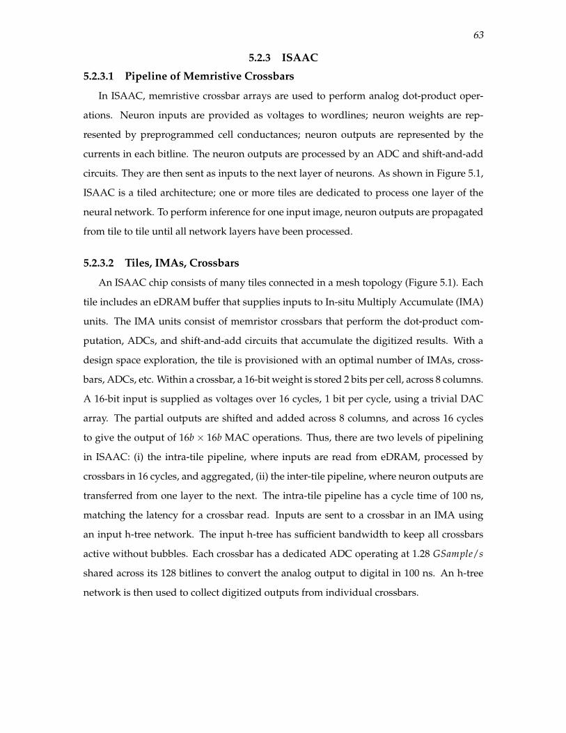
63
5.2.3 ISAAC
5.2.3.1 Pipeline of Memristive Crossbars
In ISAAC, memristive crossbar arrays are used to perform analog dot-product oper-
ations. Neuron inputs are provided as voltages to wordlines; neuron weights are rep-
resented by preprogrammed cell conductances; neuron outputs are represented by the
currents in each bitline. The neuron outputs are processed by an ADC and shift-and-add
circuits. They are then sent as inputs to the next layer of neurons. As shown in Figure 5.1,
ISAAC is a tiled architecture; one or more tiles are dedicated to process one layer of the
neural network. To perform inference for one input image, neuron outputs are propagated
from tile to tile until all network layers have been processed.
5.2.3.2 Tiles, IMAs, Crossbars
An ISAAC chip consists of many tiles connected in a mesh topology (Figure 5.1). Each
tile includes an eDRAM buffer that supplies inputs to In-situ Multiply Accumulate (IMA)
units. The IMA units consist of memristor crossbars that perform the dot-product com-
putation, ADCs, and shift-and-add circuits that accumulate the digitized results. With a
design space exploration, the tile is provisioned with an optimal number of IMAs, cross-
bars, ADCs, etc. Within a crossbar, a 16-bit weight is stored 2 bits per cell, across 8 columns.
A 16-bit input is supplied as voltages over 16 cycles, 1 bit per cycle, using a trivial DAC
array. The partial outputs are shifted and added across 8 columns, and across 16 cycles
to give the output of 16b× 16b MAC operations. Thus, there are two levels of pipelining
in ISAAC: (i) the intra-tile pipeline, where inputs are read from eDRAM, processed by
crossbars in 16 cycles, and aggregated, (ii) the inter-tile pipeline, where neuron outputs are
transferred from one layer to the next. The intra-tile pipeline has a cycle time of 100 ns,
matching the latency for a crossbar read. Inputs are sent to a crossbar in an IMA using
an input h-tree network. The input h-tree has sufficient bandwidth to keep all crossbars
active without bubbles. Each crossbar has a dedicated ADC operating at 1.28 GSample/s
shared across its 128 bitlines to convert the analog output to digital in 100 ns. An h-tree
network is then used to collect digitized outputs from individual crossbars.

64
Hyper Transport 2.0
eDRAMBank
Adders Pooling
IMA
ADC
ADC
ADC
ADC
OutReg
InReg
TILE
xbar
S+H
MUX
DA
C
Figure 5.1. The ISAAC Architecture.
5.2.3.3 Crossbar Challenges
As with any new technology, a memristor crossbar has unique challenges, mainly
in two respects. First, mapping a matrix onto a memristor crossbar array requires pro-
gramming (or writing) cells with the highest precision possible. Second, real circuits
deviate from ideal operation due to parasitics such as wire resistance, device variation,
and write/read noise. All of these factors can cause the actual output to deviate from its
ideal value. Recent work [76] has captured many of these details to show the viability of
prototypes [3]. Section 5.2.4 summarizes some of these details.
5.2.4 Crossbar Implementations
This section discusses how crossbars can be designed to withstand noise effects in
analog circuits.
5.2.4.1 Process Variation and Noise
Since an analog crossbar uses actual conductance of individual cells to perform com-
putation, it is critical to do writes at maximum precision. We make two design choices
to improve write precision. First, we equip each cell with an access transistor (1T1R cell)
to precisely control the amount of write current going through it. While this increases

65
area overhead, it eliminates sneak currents and their negative impact on write voltage
variation [200]. Second, we use a closed loop write circuit with current compliance that
does many iterations of program-and-verify operations. Prior work has shown that such
an approach can provide more precise states at the cost of increased write time even with
high process variation in cells [6].
In spite of a robust write process, a cell’s resistance will still deviate from its normal
value within a tolerable range. This range will ultimately limit either the number of levels
in a cell or the number of simultaneously active rows in a crossbar. For example, if a cell
write can achieve a resistance within ∆r (∆r is a function of noise and parasitic), if l is the
number of levels in a cell, and rrange is the max range of resistance of a cell, then we set the
number of active rows to rrange/(l.∆r) to ensure there are no corrupted bits at the ADC.
5.2.4.2 Crossbar Parasitic
While a sophisticated write circuit coupled with limited array size can help alleviate
process variation and noise, IR drop along rows and columns can also reduce crossbar
accuracy. When a crossbar is being written during initialization, the access transistors
in unselected cells shut off the sneak current path, limiting the current flow to just the
selected cells. However, when a crossbar operates in compute mode in which multiple
rows are active, the net current in the crossbar increases, and the current path becomes
more complicated. With access transistors in every cell in the selected rows in ON state,
a network of resistors is formed with every cell conducting varying current based on its
resistance. As wire links connecting these cells have nonzero resistance, the voltage drop
along rows and columns will impact the computation accuracy. Thus, a cell at the far end
of the driver will see relatively lower read voltage compared to a cell closer to the driver.
This change in voltage is a function of both wire resistance and the current flowing through
wordlines and bitlines, which in turn is a function of the data pattern in the array. This
problem can be addressed by limiting the DAC voltage range and doing data encoding
to compensate for the IR drop [76]. Since the matrix being programmed into a crossbar is
known beforehand, during the initialization phase of a crossbar, it is possible to account for
voltage drops and adjust the cell resistance appropriately. Hu et al. [76] have demonstrated
successful operation of a 256×256 crossbar with 5-bit cells even in the presense of thermal

66
noise in memristor, short noise in circuits, and random telegraphic noise in the crossbar.
For this work, a conservative model with a 128×128 crossbar with 2-bit cells and 1-bit DAC
emerges as an ideal design point in most experiments.
5.3 The Newton ArchitectureSimilar to ISAAC, Newton employs a tiled architecture, where every tile is composed
of several IMAs. Newton is targeted for mobile platforms (self-driving cars, phones) and
datacenters. In both cases, the chips will be continuously fed with inputs from several cam-
eras or users – hence our focus on throughput and energy efficiency. We first discuss three
innovations that are applied within a Newton IMA, followed by three innovations that are
applied within a Newton tile. The overarching theme in these ideas is the reduction in
ADC and resource requirements.
5.3.1 Intra-IMA Optimizations
5.3.1.1 Mapping Constraints
ISAAC did not place any constraints on how a neural network can be mapped to its
many tiles and IMAs. As a result, its resources, notably the HTree and buffers within an
IMA, are provisioned to handle the worst case. This has a negative impact on power and
area efficiency. Instead, we place constraints on how the workload is mapped to IMAs.
While this inflexibility can waste a few resources, we observe that it also significantly
reduces the HTree size and hence area per IMA. The architecture is still general-purpose,
i.e., arbitrary CNNs can be mapped to Newton.
5.3.1.2 Bit Interleaved Crossbars
The layout of an IMA with 16 crossbars is shown in Figure 5.2. We co-locate an ADC
with each crossbar. The digitized outputs are then sent to the IMA’s output register via an
HTree network. While ISAAC was agnostic to how a single synaptic weight was scattered
across multiple bitlines, we adopt the following approach to boost efficiency. A 16-bit
weight is scattered across 8 2-bit cells; each cell is placed in a different crossbar. Therefore,
crossbars 0 and 8 are responsible for the least significant bits of every weight, and crossbars
7 and 15 are responsible for the most significant bits of every weight. We also embed the
shift-and-add units in the HTree. So the shift-and-add unit at the leaf of the HTree adds

67
Out
Reg
In
Reg
S+A
S+A
S+A
S+A
S+A
S+A
S+A
S+A
S+A
S+A
S+A
S+A
S+A
S+A
MATS
DA
C
xbar 0
S+H
128:1MUX
ADC
Figure 5.2. Microarchitecture of an IMA.
the digitized 9-bit dot-product results emerging from two neighboring crossbars. Because
the operation is a shift-and-add, it produces an 11-bit result. The next shift-and-add unit
takes 2 11-bit inputs to produce a 13-bit input, and so on. In addition to being an efficient
pipeline, and lowering the HTree widths, this approach lends itself to the heterogeneity
measures we introduce shortly.
5.3.1.3 An IMA as an Indivisible Resource
We further introduce the constraint that an IMA cannot be shared by multiple net-
work layers. If multiple layers were to share an IMA, we would need multiple HTrees to
support the simultaneous aggregation of multiple neurons. This introduces a nontrivial
area overhead, and offers a flexibility that is rarely useful to the workloads we examined.
An IMA therefore represents an indivisible resource unit that is allocated to a network
layer. We also restrict the number of inputs (128) to an IMA to boost input sharing and
reduce HTree bandwidth and input buffering requirements. By placing these constraints,
depending on the sizes of network layers, a few crossbars in a few IMAs go unutilized,
but for our workloads, this is minor and not enough to offset the power/area benefit of a
smaller HTree.
5.3.1.4 Adaptive ADCs
We will first take a closer look at the dot-product being performed within an IMA.
As with prior work, we are performing dot-products on 16-bit fixed-point neurons and
weights, with a fixed-point scaling factor of 210. A 16-bit weight is spread across 8 cells

68
(each in a different crossbar). The 16-bit input is iteratively fed as 16 1-bit inputs. In a single
iteration, a crossbar column is performing a dot-product involving 128 rows, 1-bit inputs,
and 2-bit cells; it therefore produces a 9-bit result requiring a 9-bit ADC.1 We must shift
and add the results of eight such columns, yielding a 23-bit result. These results must also
be shifted and added across 16 iterations, finally yielding a 39-bit output. Once the scaling
factor is applied, the least significant 10 bits are dropped. The most significant 13 bits
represent an overflow that cannot be captured in the 16-bit result, so they are effectively
used to clamp the result to a maximum value.
What is of note here is that the output from every crossbar column in every iteration
is being resolved with a high-precision 9-bit ADC, but many of these bits contribute to
either the 10 least significant bits or the 13 most significant bits that are eventually going
to be ignored. This is an opportunity to lower the ADC precision and ignore some bits,
depending on the column and the iteration being processed. Figure 5.3 shows the number
of relevant bits emerging from every column in every iteration.
1ISAAC introduces a data encoding that can reduce the ADC resolution by 1 bit [163].
Figure 5.3. Heterogeneous ADC sampling resolution

69
The ADC accounts for a significant fraction of IMA power. When the ADC is operating
at a lower resolution, it has less work to do. In every 100 ns iteration, we tune the reso-
lution of a SAR ADC to match the requirement in Figure 5.3. Thus, the use of adaptive
ADCs helps reduce IMA power while having no impact on performance. We are also
ignoring bits that do not show up in a 16-bit fixed-point result, so we are not impacting the
functional behavior of the algorithm, thus having zero impact on algorithm accuracy.
A SAR ADC does a binary search over the input voltage to find the digital value,
starting from the MSB. A bit is set to 1, and the resulting digital value is converted to
analog and compared with the input voltage. If the input voltage is higher, the bit is set
to 1, the next bit is changed, and the process repeats. If the number of bits to be sampled
is reduced, the circuit can ignore the latter stages. The ADC simply gates off its circuits
until the next sample is provided. While we could increase sampling frequency, this is not
helpful because we can only run as fast as the slowest stage in the ISAAC pipeline. It is
important to note that the ADC starts the binary search from the MSB, and thus it is not
possible to sample just the lower significant bits of an output without knowing the MSBs.
But in this case, we have a unique advantage: if any of the MSBs to be truncated is 1, then
the output neuron value is clamped to the highest value in the fixed point range. Thus, in
order to sample a set of LSBs, the ADC starts the binary search with the LSB+1 bit. If that
comparison yields true, it means at least one of the MSB bits is 1. This signal is sent across
the HTree and the output is clamped.
In conventional SAR ADCs [189], a third of the power is dissipated in the capacitive
DAC (CDAC), a third in digital circuits, and a third in other analog circuits. The MSB
decision in general consumes more power because it involves charging up the CDAC at
the end of every sampling iteration. Recent trends show CDAC power diminishing due to
use of tiny unit capacitances (about 2fF) and innovative reference buffer designs, leading
to ADCs consuming more power in analog and digital circuits [98], [134]. The Adaptive
ADC technique is able to reduce energy consumption irrespective of the ADC design since
it eliminates both LSB and MSB tests across the 16 iterations.
Note that by interleaving a weight across multiple crossbars, we must adapt the ADC
once every 100 ns iteration, and not for every new input sample. It is also worth pointing
out that the adaptive ADC technique is compatible with the encoding used by ISAAC to

70
reduce ADC resolution by 1 bit.
5.3.1.5 Divide and Conquer Multiplication
We now introduce another technique that reduces pressure on ADC usage and hence
ADC power. This can be done with linear algebra optimizations within and outside an
IMA. Here, we discuss a divide and conquer strategy at the bit level (Karatsuba’s tech-
nique), applied within an IMA. Later, in Section 5.3.2.3, we apply a similar strategy at
matrix granularity outside an IMA (Strassen’s technique).
A classic multiplication approach for two n-bit numbers has a complexity of O(n2)
where each bit of a number is multiplied with n-bits of the other number, and the partial
results are shifted and added to get the final 2n-bit result. A similar approach is taken in
ISAAC. However the time complexity is O(n), since multiplication of 1-bit of input with
n-bits of weight happens in parallel.
Karatsuba’s divide and conquer algorithm manages to reduce the complexity from
O(n2) to O(n1.5). As shown in Figure 5.4, it divides the numbers into two halves of n/2 bits,
MSB bits and LSB bits, and instead of performing four smaller n/2-bit multiplications, it
calculates the result with two n/2-bit multiplications and one (n/2 + 1)-bit multiplication.
In baseline ISAAC, the product of input X and weight W is performed on 8 crossbars
in 16 cycles (since each weight is spread across 8 cells in 8 different crossbars and the input
is spread across 16 iterations). In the example in Figure 5.4, W0X0 is performed on four
crossbars in 8 iterations (since we are dealing with fewer bits for weights and inputs). The
same is true for W1X1. A third set of crossbars stores the weights (W1 + W0) and receives
the precomputed inputs (X1 + X0). This computation is spread across 5 crossbars and 9
WX = 2N W1X1 + 2N/2 (W
1X0+W
0X1) + W
0X0
= 2N W1X1 + 2N/2 [(W
1+W
0)(X
1+X
0)-(W
1X1+W
0X0)] + W
0X0
= (2N-1)W1X1 + 2N/2 (W
1+W
0)(X
1+X
0) + (1-2N/2)W
0X0
Divide & Conquer
W=2N/2 W1+W
0X=2N/2 X
1+X
0
Figure 5.4. Karatsuba’s Divide & Conquer Algorithm

71
iterations. We see that the total amount of work has reduced by 15%.
To implement this algorithm, we modify the IMA as shown in Figure 5.5. The changes
are localized to a single mat. Each mat now has two crossbars that share the DAC and
ADC. Given the size of the ADC, the extra crossbar per mat has a minimal impact on area.
The left crossbars in four of the mats now store W0; the left crossbars in the other four mats
store W1; the right crossbars in five of the mats store W0 + W1; the right crossbars in three
of the mats are unused. In the first 8 iterations, the 8 ADCs are used by the left crossbars.
In the next 9 iterations, 5 ADCs are used by the right crossbars. The main objective here is
to lower power by reducing use of the ADC.
There are a few drawbacks as well. A computation now takes 17 iterations instead of
16. The IMA area increases because the HTree must send inputs X0 and X1 in parallel,
each mat has an additional crossbar, the output buffer is larger to store subproducts, and
128 1-bit full adders are required to compute (X1 + X0). Again, given that the ADC is the
primary bottleneck, these other overheads are relatively minor.
Divide & Conquer can be recursively applied further. When applied again, the com-
putation keeps 8 ADCs busy in the first 4 iterations, and 6 ADCs in the next 10 iterations.
This is a 28% reduction in ADC use, and a 13% reduction in execution time. But, we pay
an area penalty because 20 crossbars are needed per IMA.
In Figure 5.3, it is evident that most ADC undersampling is done for the subproducts
X0W0 and X1W1, thus allowing the previous technique to be combined with Karatsuba’s
algorithm.
S+A
S+A
S+A
S+A
S+A
S+A
MATS
xbar 0 xbar 1
S+H
128:1MUX
S+H
Tunable
ADC
2:1MUX
128:1MUX
DA
C
S+A
In
Reg
Out
Reg
Figure 5.5. IMA supporting Karatsuba’s Algorithm.

72
5.3.2 Intra-Tile Optimizations
The previous subsection focused on techniques to improve an IMA; we now shift our
focus to the design of a tile. We first reduce the size of the eDRAM buffer that feeds all
the IMAs in a tile. We then create heterogeneous tiles that suit convolutional and fully-
connected layers. Finally, we use a divide-and-conquer approach at the tile level.
5.3.2.1 Reducing Buffer Sizes
Because ISAAC did not place constraints on how layers are mapped to crossbars and
tiles, the eDRAM buffer was sized to 64KB to accommodate the worst-case requirements
of workloads. Here, we design mapping techniques that reduce storage requirements per
tile and move that requirement closer to the average-case.
To explain the impact of mapping on buffering requirements, first consider the convo-
lutional layer shown in Figure 5.6a. Once a certain number of inputs are buffered (shown in
green and pink), the layer enters steady state; every new input pixel allows the convolution
to advance by another step. The buffer size is a constant as the convolution advances (each
new input evicts an old input that is no longer required). In every step, a subset of the
input buffer is fed as input to the crossbar to produce one pixel in each of many output
feature maps. If the crossbar is large, it is split across 2 tiles, as shown in Figure 5.6a. The
split is done so that Tile 1 manages the green buffer and green inputs, and Tile 2 manages
the pink buffer and pink inputs. Such a split means that inputs do not have to be replicated
on both tiles, and buffering requirements are low.
Now, consider an early convolutional layer. Early convolutional layers have more work
to do than later layers since they deal with larger feature maps. In ISAAC, to make the
pipeline balanced, early convolutional layers are replicated so their throughput matches
those of later layers. Figure 5.6b replicates the crossbar; one is responsible for every odd
pixel in the output feature maps, while the other is responsible for every even pixel. In any
step, both crossbars receive very similar inputs. So the same input buffer can feed both
crossbars.
If a replicated layer is large enough that it must be spread across (say) 4 tiles, we have
two options. Figure 5.6 c and d show these two options. If the odd computation is spread
across two tiles (1 and 2) and the even computation is spread across two different tiles (3

73
(a) CONVOLUTION LAYER.
GREEN AND PINK INPUTS HAVE BEEN BUFFERED. A
CUBE OF INPUTS IS FED TO THE CROSSBAR TO PRODUCE
SEVERAL OUTPUT FEATURE MAPS. THE WORK AND
INPUTS ARE PARTITIONED ACROSS TWO TILES.
O. FTR MAP 1
O. FTR MAP N
(b) REPLICATED LAYER.
SAME INPUTS ARE FED
TO TWO CROSSBARS TO
DOUBLE THRUPUT.
ODD
OUTPUT
PIXELS
EVEN
OUTPUT
PIXELS
TILE 1
TILE 2
TILE 3
TILE 4
(c) PARTITIONING THE WORK
ACROSS 4 TILES. INPUTS
HAVE TO BE REPLICATED.
TILE 1
TILE 2
TILE 3
TILE 4
TILE 1
TILE 2
TILE 3
TILE 4
(d) BETTER PARTITIONING
ACROSS 4 TILES. INPUTS
NEED NOT BE REPLICATED.
TILE 1
TILE 2
Figure 5.6. Mapping of convolutional layers to tiles
and 4), the same green inputs have to be sent to Tile 1 and Tile 3, i.e., the input buffers are
replicated. Instead, as shown in Figure 5.6d, if we co-locate the top quadrant of the odd
computation and the top quadrant of the even computation in Tile 1, the green inputs are
consumed entirely within Tile 1 and do not have to be replicated. This partitioning leads
to the minimum buffer requirement.
The bottom line from this mapping is that when a layer is replicated, the buffering
requirements per neuron and per tile are reduced. This is because multiple neurons that
receive similar inputs can reuse the contents of the input buffer. Therefore, heavily repli-
cated (early) layers have lower buffer requirements per tile than lightly replicated (later)
layers. If we mapped these layers to tiles as shown in Figure 5.7a, the worst-case buffering
requirement goes up (64 KB for the last layer), and early layers end up under-utilizing
their 64 KB buffer. To reduce the worst-case requirement and the under-utilization, we
instead map layers to tiles as shown in Figure 5.7b. Every layer is finely partitioned and
spread across 10 tiles, and every tile maps part of a layer. By spreading each layer across many
tiles, every tile can enjoy the buffering efficiency of early layers. By moving every tile’s buffer
requirement closer to the average-case (21 KB in this example), we can design a Newton
tile with a smaller eDRAM buffer (21 KB instead of 64 KB) that achieves higher overall
computational efficiency. This does increase the inter-tile neuron communication, but this
has a relatively small impact on computational efficiency.
5.3.2.2 Different Tiles for Convolutions and Classifiers
While ISAAC uses the same homogeneous tile for the entire chip, we observe that
convolutional layers have very different resource demands than fully-connected classifier

74
LAYER 1 ON TILES 1-4
8X REPLICATION
BUFFER / TILE: 8KB
LAYER 2 ON TILES 5-7
4X REPLICATION
BUFFER / TILE: 16KB
LAYER 3 ON TILES 8-9
2X REPLICATION
BUFFER / TILE: 32KB
LAYER 4 ON TILE 10
1X REPLICATION
BUFFER / TILE: 64KB
(a) ASSIGN TILES TO LAYERS
LAYER 1 ON TILES 1-10
8X REPLICATION
LAYER 2 ON TILES 1-10
4X REPLICATION
LAYER 3 ON TILES 1-10
2X REPLICATION
LAYER 4 ON TILES 1-10
1X REPLICATION
(b) SPREAD A LAYER ACROSS ALL TILES. BUFFER / TILE : 21KB.
Figure 5.7. Mapping layers to tiles for small buffer sizes.
layers. The classifier (or FC) layer has to aggregate a set of inputs required by a set of
crossbars; the crossbars then perform their computation; the inputs are discarded and a
new set of inputs is aggregated. This results in the following properties for the classifier
layer:
1. The classifier layer has a high communication-to-compute ratio, so the router band-
width puts a limit on how often the crossbars can be busy.
2. The classifier also has the highest synaptic weight requirement because every neuron
has private weights.
3. The classifier has low buffering requirements – an input is seen by several neurons
in parallel, and the input can be discarded right after.
We therefore design special Newton tiles customized for classifier layers that:
1. have a higher crossbar-to-ADC ratio (4:1 instead of 1:1),

75
2. operate the ADC at a lower rate (10 Msamples/sec instead of 1.2 Gsamples/sec),
3. have a smaller eDRAM buffer size (4 KB instead of 16 KB).
For small-scale workloads that are trying to fit on a single chip, we would design a chip
where many of the tiles are conv-tiles and some are classifier-tiles (a ratio of 1:1 is a good
fit for most of our workloads). For large-scale workloads that use multiple chips, each chip
can be homogeneous; we use roughly an equal number of conv-chips and classifier-chips.
The results consider both cases.
5.3.2.3 Strassen’s Algorithm
A divide and conquer approach can also be applied to matrix-matrix multiplication.
Note that all of our computations are vector-matrix multiplications. But when a layer is
replicated, multiple input vectors are being fed to the same matrix of weights; so repli-
cated layer computations are matrix-matrix multiplications. By partitioning each matrix
X and W into 4 submatrices, we can express matrix-matrix multiplication in terms of
multiplications of submatrices. The typical algorithm, assumed in ISAAC, would require
8 submatrix multiplications, followed by an aggregation step. But as shown in Figure 5.8,
linear algebra manipulations can perform the same computation with 7 submatrix mul-
tiplications, with appropriate pre and postprocessing. Similar to Karatsuba’s algorithm,
this has the advantage of reducing ADC usage and power. As shown in Figure 5.9, the
computations (P0 − P6) in Strassen’s algorithm are mapped to 7 IMAs in the tile. The 8th
IMA can be allocated to another layer’s computation. While both divide and conquer
algorithms (Karatsuba’s within an IMA and Strassen’s within a tile) are highly effective
for a crossbar-based architecture, they have very little impact on other digital accelerators.
For example, these algorithms may impact the efficiency of the NFUs in DaDianNao, but
DaDianNao area is dominated by eDRAM banks and not NFUs. In fact, Strassen’s algo-
rithm can lower DaDianNao efficiency because buffering requirements may increase. On
the other hand, the computations in Newton are linked with expensive ADCs, so efficient
computation does noticeably impact overall efficiency. Further, some of the preprocessing
for these algorithms is performed when installing weights on the Newton chip, but has to
be performed on-the-fly for digital accelerators.
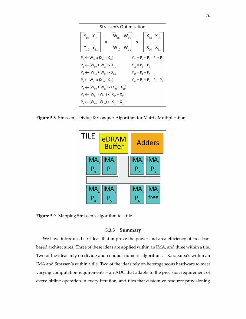
76
Y00
Y01
Y10
Y11
Y00
= P4 + P
3 - P
1 + P
5
Y01
= P0 + P
1
Y10
= P2 + P
3
Y11
= P0 + P
4 - P
2 - P
6
= x
W00
W01
W10
W11
X00
X01
X10
X11
P0 W
00 x (X
01 - X
11)
P1 (W
00 + W
01) x X
11
P2 (W
10 + W
11) x X
00
P3 W
11 x (X
10 - X
00)
P4 (W
00 + W
11) x (X
00 + X
11)
P5 (W
01 - W
11) x (X
10 + X
11)
P6 (W
00 - W
10) x (X
00 + X
01)
Strassen’s Op!miza!on
Figure 5.8. Strassen’s Divide & Conquer Algorithm for Matrix Multiplication.
eDRAM
BufferAdders
P0
IMA0
P1
IMA1
P2
IMA2
P3
IMA3
P4
IMA4
P5
IMA5
P6
IMA6IMA
7
TILE
free
Figure 5.9. Mapping Strassen’s algorithm to a tile.
5.3.3 Summary
We have introduced six ideas that improve the power and area efficiency of crossbar-
based architectures. Three of these ideas are applied within an IMA, and three within a tile.
Two of the ideas rely on divide-and-conquer numeric algorithms – Karatsuba’s within an
IMA and Strassen’s within a tile. Two of the ideas rely on heterogeneous hardware to meet
varying computation requirements – an ADC that adapts to the precision requirement of
every bitline operation in every iteration, and tiles that customize resource provisioning
77
for classifier layers. Two of the ideas introduce constraints on how network layers are
mapped to resources – by introducing constraints within an IMA, we reduce HTree size –
by spreading a layer across many tiles, we reduce the eDRAM buffer requirements. Note
again that these constraints do not limit generality and any CNN can be mapped to a
sufficiently large collection of Newton tiles.
5.4 Methodology5.4.1 Modeling Area and Energy
For modeling the energy and area of the eDRAM buffers and on-chip interconnect like
the HTree and tile bus, we use CACTI 6.5 [133] at 32 nm. The area and energy model
of a memristor crossbar is based on [76]. We adapt the area and energy of shift-and-add
circuits, max/average pooling block and sigmoid operation similar to the analysis in Da-
DianNao [32] and ISAAC [163]. We avail the same HyperTransport serial link model for
off-chip interconnects as used by DaDianNao [32] and ISAAC [32]. The router area and
energy is modeled using Orion 2.0 [82]. While our buffers can also be implemented with
SRAM, we use eDRAM to make an apples-to-apples comparison with the ISAAC baseline.
Newton is only used for inference, with a delay of 16.4 ms to preload weights in a chip.
In order to model the ADC energy and area, we use a recent survey [134] of ADC
circuits published in different circuit conferences. The Newton architecture uses the same
8-bit ADC [98] at 32 nm as used in ISAAC, partly because it yields the best configuration in
terms of area/power and meets the sampling frequency requirement, and partly because
it can be reconfigured for different resolutions. This is at the cost of minimal increase in
area of the ADC. We scale the ADC power with respect to different sampling frequency
according to another work by Kull et al. [98]. The SAR ADC has six different components:
comparators, asynchronous clock logic, sampling clock logic, data memory and state logic,
reference buffer, and capacitive DAC. The ADC power for different sampling resolution is
modeled by gating off the other components except the sampling clock.
We consider a 1-bit DAC as used in ISAAC because it is relatively small and has high
SNR value. Since DAC is used in every row of the crossbar, a 1-bit DAC improves the area
efficiency.
The key parameters in the architecture that largely contribute to our analysis are re-

78
ported in Table 5.1.
This work considers recent workloads with state-of-the-art accuracy in image classifi-
cation tasks (summarized in Table 5.2). We create an analytic model for a Newton pipeline
within an IMA and within a tile and map the suite of benchmarks, making sure that
there are no structural hazards in any of these pipelines. We consider network bandwidth
limitations in our simulation model to estimate throughput. Since ISAAC is a throughput
architecture, we do an iso-throughput comparison of the Newton architecture with ISAAC
for the different intra-IMA or intra-tile optimizations. Since the dataflow in the architecture
is bounded by the router bandwidth, in each case, we allocate enough resources until the
network saturates to create our baseline model. For subsequent optimizations, we retain
the same throughput. Similar to ISAAC, data transfers between tiles on-chip, and on the
HT link across chips have been statically routed to make it conflict free. Like ISAAC, the
latency and throughput of Newton for the given benchmarks can be calculated analytically
using a deterministic execution model. Since there aren’t any run-time dependencies on
the control flow or data flow of the deep networks, analytical estimates are enough to
capture the behavior of cycle-accurate simulations.
We create a similar model for ISAAC, taking into considerations all the parameters
mentioned in their work.
5.4.2 Design Points
The Newton architecture can be designed by optimizing one of the following two
metrics:
1. CE: Computational Efficiency which is the number of fixed point operations per-
formed per second per unit area, GOPS/(s×mm2).
Table 5.1. Key contributing elements in Newton.
Component Spec Power Area (mm2)Router 32 flits, 8 ports 168 mW 0.604ADC 8-bit resolution 3.1 mW 0.0015
1.2 GSps frequencyHyper Tr 4 links @ 1.6GHz 10.4 W 22.88
6.4 GB/s link bwDAC array 128 1-bit resolution 0.5 mW 0.00002
number 8× 128Memristor crossbar 128× 128 0.3 mW 0.000025
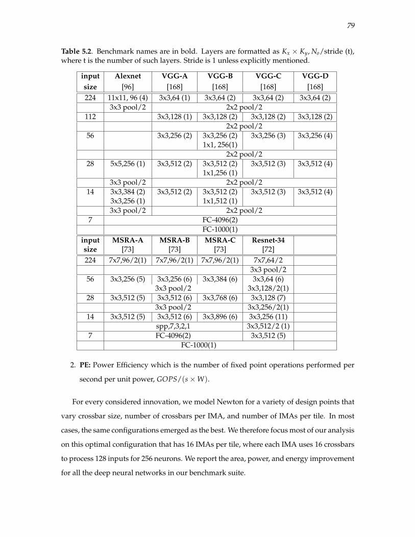
79
Table 5.2. Benchmark names are in bold. Layers are formatted as Kx × Ky, No/stride (t),where t is the number of such layers. Stride is 1 unless explicitly mentioned.
input Alexnet VGG-A VGG-B VGG-C VGG-Dsize [96] [168] [168] [168] [168]224 11x11, 96 (4) 3x3,64 (1) 3x3,64 (2) 3x3,64 (2) 3x3,64 (2)
3x3 pool/2 2x2 pool/2112 3x3,128 (1) 3x3,128 (2) 3x3,128 (2) 3x3,128 (2)
2x2 pool/256 3x3,256 (2) 3x3,256 (2) 3x3,256 (3) 3x3,256 (4)
1x1, 256(1)2x2 pool/2
28 5x5,256 (1) 3x3,512 (2) 3x3,512 (2) 3x3,512 (3) 3x3,512 (4)1x1,256 (1)
3x3 pool/2 2x2 pool/214 3x3,384 (2) 3x3,512 (2) 3x3,512 (2) 3x3,512 (3) 3x3,512 (4)
3x3,256 (1) 1x1,512 (1)3x3 pool/2 2x2 pool/2
7 FC-4096(2)FC-1000(1)
input MSRA-A MSRA-B MSRA-C Resnet-34size [73] [73] [73] [72]224 7x7,96/2(1) 7x7,96/2(1) 7x7,96/2(1) 7x7,64/2
3x3 pool/256 3x3,256 (5) 3x3,256 (6) 3x3,384 (6) 3x3,64 (6)
3x3 pool/2 3x3,128/2(1)28 3x3,512 (5) 3x3,512 (6) 3x3,768 (6) 3x3,128 (7)
3x3 pool/2 3x3,256/2(1)14 3x3,512 (5) 3x3,512 (6) 3x3,896 (6) 3x3,256 (11)
spp,7,3,2,1 3x3,512/2 (1)7 FC-4096(2) 3x3,512 (5)
FC-1000(1)
2. PE: Power Efficiency which is the number of fixed point operations performed per
second per unit power, GOPS/(s×W).
For every considered innovation, we model Newton for a variety of design points that
vary crossbar size, number of crossbars per IMA, and number of IMAs per tile. In most
cases, the same configurations emerged as the best. We therefore focus most of our analysis
on this optimal configuration that has 16 IMAs per tile, where each IMA uses 16 crossbars
to process 128 inputs for 256 neurons. We report the area, power, and energy improvement
for all the deep neural networks in our benchmark suite.

80
5.5 ResultsAs we move through the results, we will incrementally add each innovation. Each
reported improvement is relative to the Newton architecture with innovations described
until that point.
5.5.1 Constrained Mapping for Compact HTree
The Newton architecture takes the baseline analog accelerator ISAAC and incremen-
tally applies a series of techniques. We first observe that the ISAAC IMA is designed with
an over-provisioned HTree that can handle a worst-case mapping of the workload. We
imposed the constraint that an IMA can only handle a single layer, and a maximum of
128 inputs. This restricts the width of the HTree, promotes input sharing, and enables
reduction of partial neuron values at the junctions of the HTree. While this helps shrink
the size of an IMA, it suffers from crossbar under-utilization within an IMA. We con-
sider different IMA sizes, ranging from 128 × 64 which supplies the same 128 neurons
to 4 crossbars to get 64 output neurons, to 8192 × 1024. Figure 5.10 plots the average
under-utilization of crossbars across the different workloads in the benchmark suite. For
larger IMA sizes, the under-utilization is quite significant. Larger IMA sizes also result
in complex HTrees. Therefore, a moderately sized IMA that processes 128 inputs for
256 neurons has high computational efficiency and low crossbar under-utilization. For
this design, the under-utilization is only 9%. Figure 5.11 quantifies how our constrained
mapping and compact HTree improve area, power, and energy per workload. In short,
our constraints have improved area efficiency by 37% and power/energy efficiency by
18%, while leaving only 9% of crossbars under-utilized.
5.5.2 Heterogeneous ADC Sampling
The heteregenous sampling of outputs using adaptive ADCs has a big impact on re-
ducing the power profile of the analog accelerator. In one iteration of 100 ns, at max 4
ADCs work at the max resolution of 8-bits. Power supply to the rest of the ADCs can be
reduced. We measure the reduction of area, power, and energy with respect to the new
IMA design with the compact HTree. Since ADC contributed to 49% of the chip power
in ISAAC, reducing the oversampling of ADC reduces power requirement by 15% on

81
Figure 5.10. Crossbar under-utilization with constrained mapping.
Figure 5.11. Impact of constrained mapping and compact HTree.
average. The area efficiency improves as well since the output-HTree now carries 16 bits
instead of unnecessarily carrying 39 bits of final output. The improvements are shown in
Figure 5.12.
5.5.3 Karatsuba’s Algorithm
We further try to reduce the power profile with divide-and-conquer within an IMA.
Figure 5.13 shows the impact of recursively applying the divide-and-conquer technique
multiple times. Applying it once is nearly as good as applying it twice, and much less
complex. Therefore, we focus on a single divide-and-conquer step. Improvements are
reported in Figure 5.14. Energy efficiency improves by almost 25% over the previous
design point, because ADCs end up being used 75% of the times in the 1700 ns window.
However, this comes at a cost of 6.4% reduction in area efficiency because of the need for
more crossbars and increase in HTree bandwidth to send the sum of inputs.

82
Figure 5.12. Improvement due to the adaptive ADC scheme.
Figure 5.13. Comparison of CE and PE for Divide and Conquer done recursively.
Figure 5.14. Improvement with Karatsuba’s Algorithm.

83
5.5.4 eDRAM Buffer Requirements
In Figure 5.15, we report the buffer requirement per tile when the layers are spread
across many tiles. We consider this for a variety of tile/IMA configurations. Even though
this plot pertains to the workloads considered in this chapter, as long as the image sizes
processed by the network remain 256 × 256 or below, it is highly representative of all
workloads. Image size has a linear impact on the buffering requirement. This observation
leads to the choice of a 16 KB buffer instead of the 64 KB used in ISAAC, a 75% reduction.
Figure 5.16 shows 6.5% average improvement in area efficiency because of the buffer
reduction.
5.5.5 Conv-Tiles and Classifier-Tiles
Figure 5.17 plots the decrease in power requirement when FC tiles are operated at
8×, 32× and 128× slower than the conv tiles. None of these configurations lowers the
throughput as the FC layer is not on the critical path. Since ADC power scales linearly
with sampling resolution, the power profile is lowest when the ADCs work 128× slower.
This leads to 50% lower peak power on average. In Figure 5.18, we plot the increase in area
efficiency when multiple crossbars share the same ADC in FC tiles. The under-utilization
of FC tiles provides room for making them storage efficient, saving on average 38% of chip
area. We do not increase the ratio beyond 4 because the multiplexer connecting the cross-
bars to the ADC becomes complex. Resnet does not gain much from the heterogeneous
tiles because it needs relatively fewer FC tiles.
5.5.6 Strassen’s Algorithm
Strassen’s optimization is especially useful when large matrix multiplication can be
performed in the conv layers without much wastage of crossbars. This provides room for
decomposition of these large matrices, which is the key part of Strassen’s technique. We
note that Resnet has high wastage when using larger IMAs, and thus does not benefit at all
from this technique. Overall, Strassen’s algorithm increases the energy efficiency by 4.5%
as seen in Figure 5.19.

84
Figure 5.15. Buffer requirements for different tiles, changing the type of IMA and thenumber of IMAs.
Figure 5.16. Improvement in area efficiency with decreased eDRAM buffer sizes.
Figure 5.17. Decrease in power requirement when frequency of FC tiles is altered.

85
Figure 5.18. Improvement in area efficiency when sharing multiple crossbars per ADC inFC tiles.
Figure 5.19. Improvement due to the Strassen technique.
5.5.7 Putting it All Together
Figure 5.20 plots the incremental effect of each of our techniques on peak computational
and power efficiency of DaDianNao, ISAAC, and Newton. We do not include the hetero-
geneous FC tile in this plot because it is forcibly operated slowly because it is noncritical;
as a result, its peak throughput is lower by definition. We see that both adaptive ADC
and Divide & Conquer play a significant role in increasing the PE. While the impact of
Strassen’s technique is not visible in this graph, it manages to free up resources (1 every 8
IMA) in a tile, thus providing room for more compact mapping of networks, and reducing
ADC utilization.
Figure 5.21 shows a per-benchmark improvement in area efficiency and the contri-

86
Figure 5.20. Peak CE and PE metrics of different schemes along with baseline digital andanalog accelerator.
Figure 5.21. Breakdown of area efficiency.
bution of each of our techniques. The compact HTree and the FC tiles are the biggest
contributors. Figure 5.22 similarly shows a breakdown for decrease in power envelope,
and Figure 5.23 does the same for improvement in energy efficiency. Multiple innovations
(HTree, adaptive ADC, Karatsuba, FC tiles) contribute equally to the improvements. We
also observed that the Adaptive ADC technique’s improvement is not very sensitive to
the ADC design. We evaluated ADCs where the CDAC power dissipates 10% and 27% of
ADC power; the corresponding improvements with the Adaptive ADC were 13% and 12%
respectively.

87
Figure 5.22. Breakdown of decrease in power envelope.
Figure 5.23. Breakdown of energy efficiency.
5.6 ConclusionsIn this work, we target resource provisioning and efficiency in a crossbar-based deep
network accelerator. Starting with the ISAAC architecture, we show that three approaches
– heterogeneity, mapping constraints, and Divide & Conquer – can be applied within a tile
and within an IMA. This results in smaller eDRAM buffers, smaller HTree, energy-efficient
ADCs with varying resolution, energy- and area-efficiency in classifier layers, and fewer
computations. Many of these ideas would also apply to a general accelerator for matrix-
matrix multiplication, as well as to other neural networks such as RNN, LSTM, etc. The
Newton architecture cuts the current gap between ISAAC and an ideal neuron in half.
CHAPTER 6
ACCELERATING TRAINING PHASE
6.1 IntroductionTraining DNNs with large datasets takes a significant amount of time and is a major
bottleneck in the field of deep learning. To accelerate the training phase, many GPUs are
deployed to mitigate the runtime from many months to many weeks. In addition, the long
runtime of deep learning algorithms avoids a comprehensive design space exploration.
Therefore, the training phase is a good candidate for hardware acceleration. In this section,
we review the architectural requirement for such accelerators. We revisit our mixed signal
accelerator, ISAAC, and investigate the challenges for training.
ISAAC suffers from the following major hurdles during training:
1. ISAAC is made of memristor crossbars, which have limited endurance and consume
a lot of energy in writing, particularly for multilevel cells. This problem is exac-
erbated by using analog circuits, which requires an MLC (MultiLevel Cell) writing
scheme.
2. ISAAC takes advantage of fixed point operations. Fixed point-based neural networks
can achieve, or even exceed, the accuracy of floating-point-based ones in the infer-
ence mode. However, in the training phase, in every minibatch, a very small gradient
update is added to each weight that requires high-resolution operations. As a result,
fixed point operations fail to achieve the accuracy of floating point ones.
3. In contrast to the inference mode, the intermediate result should be stored, as they
are required for calculating the gradients. Therefore, training architectures can no
longer rely on pipeline structures such as the one used in ISAAC.
In this section, we investigate these challenges and review the impact of addressing them
on the design of a training accelerator based on in-situ computing. It is worth noting that

89
our analysis in this section is limited to MLPs and CNN-based networks. For other deep
networks such as RBMs (Restricted Boltzmann Machines) that have different structure and
low-resolution weights, in-situ computing might lead to different results.
6.2 The Challenge of Writing to CellsA Memristor cell offers a wide range of resistance. Therefore, it can store up to 6 bits
per cell or can be used to make memristor crossbars, for analog computing, with high-
resolution (up to 8 bits [76]) per column output. However, these features are available at
the cost of a complicated cell programming. The cost is two-fold: calculating the resistance
values and writing them.
For analog computing in a memristor crossbar, Hu et al. have shown that the conduc-
tance value for each cell depends on the neighboring cells [76]. In other words, two cells
storing the same values might be programmed to different conductance values, based on
their locations in the crossbar. More specifically, when the adjacent cells change, the current
passing through them will change, consequently. This alters the voltage value on the end of
each cell. Therefore, to maintain the current such that it performs 1-bit product operation
correctly, we have to tune the conductance values appropriately. It takes 1 second for
the software implementation of the procedure to find the conductance values. Even if
accelerated three orders of magnitudes using a specialized hardware unit, it will still take
1 msec [76]. In addition, after programming these new conductance values, we have to
verify the result. For a 128× 128 crossbar, there are 2128 possible inputs. Even trying just
1000 input samples takes 1000× 128ns = 128µsec in an analog accelerator. In addition, we
have to verify the result with the outputs of digital circuits; this new circuit also occupies
some area and takes some time to run.
The second issue is the limited number of writes per cell. This number for a crossbar
is in the range of 106 to 1010 writes per cell [48]. For the MLC write scheme, HPE lab, the
industry pioneer of memristor cell development, recently has shown that 106 writes for
analog computing is feasible [126]. However, it is worth mentioning that these numbers
are achieved in laboratories and are susceptible to decline in a large-scale fabrication.
We will see the impact of write scheme in the training phase, later in Section 6.4. The
endurance limitation makes two major obstacles for in-situ computing-based training:

90
1. Even in an SLC-based memristor crossbar, the accurate conductance value should
be programmed for signal integrity issue [76]. In addition, MLC write scheme can take
much longer than writing SLC. Merced et al. have reported 100ns to 900ns (i.e., 1 to 9 100ns
programming pulses) write times depending on the conductance accuracy of the cells.
2. In the SGD-based training, the number of times that kernel weights are updated
increases linearly with the training set size. During the last two decades, the number of
training samples has been increasing from 60,000 labeled samples in MNIST to more than
1 million images in Imagenet. This number increases by an order of magnitude when
unlabeled samples are also counted. For example, Imagenet and CIFAR have 14 million
and 80 million samples. In addition, Yahoo recently announced the releasing of huge data
set collected from 20 million users. Mao et al. released a new dataset with more than 40
million images captioned by more than 300 million sentences [122]. In addition, there are
other ways to increase the number of samples in the training phase. Here we mention two
such techniques.
1. Using GANs (Generative Adversarial Network): GANs consist of two neural net-
works G and D. G tries to learn the data distribution and D tries to find out if a
sample belongs to the training samples or was generated by G. The generative model
can later be used to produce more samples from each training sample [209].
2. Unsupervised Learning Approaches: In these approaches, the network tries to learn
regardless of the existence of labels. For instance, Sajjadi et al. [160] used one labeled
data and generated some samples from it, using data augmentation techniques. Since
all of these samples have the same label, they used a loss function that reduces the
error between the result of all the samples. In other words, they tried to maximize
the similarity between the sample originated from one labeled training data. To this
end, they generated 5 to 10 new samples per training data.
Both of the above techniques increase the number of samples in the training phase. In
general, for a sample set of size S and minibatch of size B, training with over E epochs
leads to S×EB weight updates. For large datasets, S can be around 107 to 108, B can be
around 128, and E can be around 10. This makes the number of possible trainings on a
large dataset very limited.

91
6.3 The Challenge of Fixed Point OperationsFixed point operations have been an attractive option since the time of the first VLSI-
level implementations of neural networks. However, a fixed point operation has a limited
accuracy. For a trained network, it has been observed that due to its redundancies, the final
output is not very sensitive to the numerical precision. There have been many proposals
trying to approximate a pretrained network to perform with limited fixed-point (even
binary weights) numbers without a significant loss in the accuracy. We have reviewed
some of these works in the related work chapter.
Some solutions (e.g., modified weight perturbation) in 90s suggested low-precision
operation also works for training. However, the target neural networks were small both in
the depth and the number of neurons per layer. In today's supervised learning algorithms,
millions of training samples are learned by the networks during 100K to millions of iter-
ations. In each iteration, weights are slightly updated, which might not be captured by
limited precision fixed point operations, as demonstrated below. Therefore, floating point
operations are preferred. Even the current Nvidia GPUs customized for machine learning
algorithms, still support floating point operations in their tensor cores [140].
As evidence of the above claim, it is worth mentioning a recent work , DoReFa-Net, that
focuses entirely on using the fixed point operations during training [205]. DoReFa-Net
achieves promising numbers for shallower networks (such as Alexnet) or deeper networks
with a small data set (such as ResNet-18 with CIFAR-10). Unfortunately, for large data sets
such as ImageNet on deep networks they could not reach the accuracy of float pointing-
base networks (i.e., 60% vs. 73% Top-1 accuracy on ResNet-18 for ImageNet). The gap is
expected to increase for deeper networks.
6.4 Performance LimitationsIn this section, we review the training process of a 4096-to-4096 fully-connected layer
for both an ISAAC-based architecture and DaDianNao-based architecture. Jouppi et al.
showed that such a large fully-connected layer is the dominant layer of the DNNs that run
on datacenters [80]. Through this calculation, we observe the performance weaknesses
that hinder in-situ computing to achieve better results than digital architectures in the
training phase. We will show that the memory transfer of the intermediate results takes

92
most of the time.
A 4096-to-4096 FC layer has 32MB of the parameters. We also assume that there are
256 inputs per training minibatches. Since training is memory bound, we assume two
DDR4 channels to provide 32GB/s memory bandwidth for both the ISAAC-based and
DaDianNao-based accelerators.
The training has four steps: (1) forward path, (2) backward path, (3) gradient calcula-
tion, and (4) updating the weight. In this example, we show that while in-situ computing
outperforms in Step 1 and Step 2, it cannot update weights as fast as the digital architec-
ture. In addition, we show the gradient calculation takes a large fraction of the training
time.
In ISAAC, the FC layer occupies 88 tiles (each contains 12 IMAs, with 16KB of kernel
weights per IMAs) . The tiles will be arranged in a 8× 11 rectangle. In each column of
tiles, the result of one calculation is sent to the next tile. The pipeline latency of ISAAC is
16× 128ns× 8 = 16µsec. Once the pipeline is full, every 16× 128ns = 2µsec the result of
a single input will be ready. Therefore, for 256 inputs in the batch, it takes 255× 2µsec +
16µsec = 526µsec to finish the forward path. It also takes the same amount of time to
perform the backward propagation.
For DaDianNao, this time is around 1msec, which is 2x worse than ISAAC. Hence
ISAAC can boost the forward and backward paths, which save 1msec. However, the
next step takes a longer time, which reduces the total improvement. More precisely, in
the process of calculating the gradient, a few variables per gradient should be fetched.
For example, the gradient update algorithm ADAM shown in Eq. 6.1 [93] needs to fetch
moment (mt) and raw moment (νt) for calculating the gradient. In this equation, the final
update value θt at time t is calculated based on the gradient gt and auxiliary variables mt
and νt. The fetch phase takes around 2×32MB32GBps = 2msec. These variables should also be
saved back in the memory, which takes 2 more msecs. In addition, the gradient update
involves slow operators such as division. Even if we provide enough resources for such
nontrivial operations, it still needs 4 msec, which is similar for both the ISAAC-based and
DaDianNao-based design.
The last step is to update the weights. In DaDianNao, the 128-bit central tree between
the tiles limits updating the weights to 32MB128Gbps = 2msec. For ISAAC the update overhead

93
has two parts: finding the new weights and programming the cells. we showed that,
with very optimistic assumption, it takes 1.3 msec (see section 6.2). The cell program-
ming part depends on the number of drivers per crossbar. Since we are updating the
gradients, not all the bits need a modification. If only LSB bits require a modification
then in each crossbar, one has to update 128×1288 = 2048 bits. Since each write takes
1µsec [126], it take 2msec to update all modified bits. Note that one can increase the
number of drivers. However, a write driver takes 1500µm2 area [126]. On the other
hand, having two drivers per crossbar reduces the area efficiency by 75%. This affects
ISAAC's improvements in forward and backward path (Step 1 and Step2). Therefore, we
assume one driver per crossbar. As a result, it takes at least 3.3msecs to update the weights.
The total time for ISAAC is 1msec( f orward + backward) + 4msec(gradient calculation) +
3.3msec(weightupdate) = 8.3msec. For DaDianNao, it takes 2msec( f orward + backward) +
4msec(gradientcalculation) + 2msec(weightupdate) = 8msec. In other words, the update
time nullifies the improvement in the forward and backward phases.
mt = β1 ×mt−1 + (1− β1)× gt
νt = β2 × νt−1 + (1− β22)× gt
mt =mt
1− βt1
νt =νt
1− βt2
θt = θt−1 − αmt√νt + ε
(6.1)
6.5 ConclusionIn this chapter, we investigate the potential of in-situ computing for the training phase
of DNNs. We show that an in-situ computing-based design cannot outperform digital
accelerators for three main reasons. First, the memristor cells have limited endurance and
it takes a large amount of time for programming these cells. Second, in-situ computing
relies on fixed point operations, which limits the DNN accuracy in the training mode.
Finally, training takes a significant amount of time to fetch and write back the intermediate
results.

CHAPTER 7
CONCLUSIONS
In this chapter, we review our contributions, draw final conclusions, and then briefly
explain some potential future work.
7.1 ContributionIn Chapter 2, we reviewed some commonly used layers in DNNs and observed that
matrix-by-vector multiplication (MVM) is the key operation in them. MVM requires many
sum-of-product or dot product operations and demands high memory bandwidth to fetch
the matrix.
In Chapter 4, we introduced ISAAC, a mixed-signal architecture based on in-situ com-
puting. We showed that memristor crossbars can both store the kernels and perform the
dot product operations. Additionally, we modeled ISAAC and observed that ADCs are the
main bottleneck for in-situ computing. We proposed a new data encoding that improves
crossbar throughput by a factor of two. Finally, we showed how to mitigate the on-chip
storage needed for the intermediate results. ISAAC shows in-situ computing designs can
outperform DNN digital accelerators, if they leverage pipelining, smart encodings, and
can distribute a computation in time, within crossbars, and across crossbars. In spite of
the ADC bottleneck, ISAAC is able to out-perform the computational efficiency of DaDi-
anNao by 8x. In the ISAAC design, roughly half the chip area/power can be attributed
to the ADC, i.e., it remains the key design challenge in mixed-signal accelerators for deep
networks.
In Chapter 5, we introduced Newton, an improved version of ISAAC that specifically
addresses the ADC bottleneck. Newton introduced heterogeneity in the tiles and allocated
some dense tiles for FC layers. In addition, we showed a divide-and-conquer based ap-
proach to reduce the ADC pressure. Finally, Newton used a modified kernel mapping to
improve its resource efficiency. We show that with a number of combined techniques, we

95
can bump up the efficiency of in-situ computing by an additional 2x. This helps bring the
energy-per-neuron to within 2x of an idealized neuron.
In Chapter 6, we investigate the potential of in-situ computing for the training phase.
Using a simple example of an FC layer training, we showed that digital accelerators are
more suitable for training. We enumerate three major reasons: (i) the limited endurance of
memristor cells, (ii) the demand for floating point operations during the gradient updates,
and (iii) the fact that most of the training time will be spent on the nontrivial operations as
well as the data transfer between the accelerator and the memory system.
We have thus quantified the potential improvement with in-situ mixed-signal comput-
ing for deep networks. Not only did we show nearly an order of magnitude improvement
with a first-generation design, ISAAC, we also showed that a second-generation design,
Newton, can employ many simple techniques to further make the design compelling.
We have thus shown that the improvements are significant enough that this approach is
worth pursuing by industry (even if the realities of commercial production start to shave
away some of the benefits). Indeed, prototypes are being created within HPE Labs [54].
However, this is an approach that will face a few challenges. As we point out, these
accelerators may not be competitive for training. They may also have to prove their ability
to tolerate noise in production settings.
7.2 Future WorkWe believe there are four important possible directions of research for in-situ computing-
based accelerators.
First, we observed that ADCs consume 50% of the accelerator’s power. Unfortunately,
naively reducing the resolution leads to a loss in accuracy. To support both high accuracy
in DNNs and low resolution in ADCs, the training algorithm should be modified. In other
words, the network should be redesigned based on supporting low-precision weights and
low-precision sum-of-product operations.
Second, we can extend analog computing to support sparse operations. While in-situ
computing can perform large dot products efficiently, the efficiency improvement declines
if many of the values are zeroes. To support sparsity, it requires ADCs with a reconfig-
urable resolution. In addition, a new unit should be introduced to steer the appropriate
96
inputs to each crossbar, since in sparse MVMs, inputs of the nonzero elements in the matrix
are not necessarily aligned.
The third topic is customized power efficient DNNs for small devices. Recent accel-
erators for deep learning mostly optimize performance. However, in the IoT era, many
devices work on a limited power budget. Inspired by recent advancement in more effi-
cient software implementation, we can explore low-power hardware accelerators for small
devices.
Fourth we can work on very-large scale DNNs. The human brain has 100 billion
neurons with around 10K sparse synaptic connections per neuron. To simulate and achieve
human-level intelligence, large-scale neural networks are needed. As part of our future
research, we can extend my analog acceleration research in the direction of power-efficient
and large-scale neuromorphic architectures. We believe memristor-based accelerators in
the DIMM form factor are good candidates for large-scale designs. These DIMMs can be
installed in modern rack architectures similar to HPE’s architecture, the Machine, which
connects memory components of all the server blades in a rack, through photonic links
Finally, system-level integration of DNN accelerators can be a topic for future work.
While there is a large body of research on the design of deep learning accelerators, only
a few of them have focused on adopting them in data centers. We believe it is necessary
to revisit server architectures to support accelerators. In addition, we need to address OS
level challenges such as sharing accelerators among different processes and scheduling
tasks on multiple processes on an accelerator.
We believe that exploring these lines of research will unearth significant benefits from
investing in mixed-signal devices and accelerators.
REFERENCES
[1] “CNN Benchmarks,” https://github.com/soumith/convnet-benchmarks.
[2] “Matrix Template Library,” https://software.intel.com/en-us/articles/intelr-mkl-and-c-template-libraries.
[3] “The Tomorrow Show: Three New Technologies from Hewlett Packard Labs,”https://youtu.be/tABpRpBW6h0?t=18m38s.
[4] M. Abadi, A. Agarwal, P. Barham, E. Brevdo, Z. Chen, C. Citro, G. S. Corrado,A. Davis, J. Dean, M. Devin et al., “Tensorflow: Large-scale machine learning onheterogeneous distributed systems,” arXiv preprint arXiv:1603.04467, 2016.
[5] J. Albericio, P. Judd, T. Hetherington, T. Aamodt, N. Jerger, and A. Moshovos,“Cnvlutin: Zero-neuron-free deep convolutional neural network nomputing,” inProceedings of ISCA-43, 2016.
[6] F. Alibart, L. Gao, B. D. Hoskins, and D. B. Strukov, “High precision tuning of statefor memristive devices by adaptable variation-tolerant algorithm,” Nanotechnology,2012.
[7] F. Alibart, E. Zamanidoost, and D. B. Strukov, “Pattern classification by memristivecrossbar circuits using ex-situ and in-situ training,” Nature, 2013.
[8] C. Alippi and L. Briozzo, “Accuracy vs. precision in digital vlsi architectures forsignal processing,” IEEE Transactions on Computers, vol. 47, no. 4, pp. 472–477, 1998.
[9] M. Alwani, H. Chen, M. Ferdman, and P. Milder, “Fused-layer cnn accelerators,” inMicroarchitecture (MICRO), 2016 49th Annual IEEE/ACM International Symposium on.IEEE, 2016, pp. 1–12.
[10] AMD, “The Potential Disruptiveness of AMD’S Open Source Deep Learn-ing Strategy,” http://instinct.radeon.com/en-us/the-potential-disruptiveness-of-amds-open-source-deep-learning-strategy.
[11] R. Andri, L. Cavigelli, D. Rossi, and L. Benini, “Yodann: An ultra-low power con-volutional neural network accelerator based on binary weights,” in VLSI (ISVLSI),2016 IEEE Computer Society Annual Symposium on. IEEE, 2016, pp. 236–241.
[12] C. Angermueller, T. Prnamaa, L. Parts, and O. Stegle, “Deep learning for computa-tional biology,” Molecular systems biology, vol. 12, no. 7, p. 878, 2016.
[13] D. Anguita, S. Ridella, and S. Rovetta, “Worst case analysis of weight inaccuracyeffects in multilayer perceptrons,” IEEE transactions on neural networks, vol. 10, no. 2,pp. 415–418, 1999.

98
[14] S. Anwar, K. Hwang, and W. Sung, “Structured pruning of deep convolutional neu-ral networks,” ACM Journal on Emerging Technologies in Computing Systems (JETC),vol. 13, no. 3, p. 32, 2017.
[15] ATLAS, “Automatically Tuned Linear Algebra Software (ATLAS),” http://math-atlas.sourceforge.net/.
[16] D. A. Augusto, L. M. Carvalho, P. Goldfeld, A. E. Muritiba, and M. Souza, “Aperformance comparison of linear algebra libraries for sparse matrix-vector prod-uct,” Proceeding Series of the Brazilian Society of Computational and Applied Mathematics,vol. 3, no. 1, 2015.
[17] E. Azarkhish, D. Rossi, I. Loi, and L. Benini, “Neurostream: Scalable and energyefficient deep learning with smart memory cubes,” arXiv preprint arXiv:1701.06420,2017.
[18] H. Bagherinezhad, M. Rastegari, and A. Farhadi, “Lcnn: Lookup-based convolu-tional neural network,” arXiv preprint arXiv:1611.06473, 2016.
[19] D. Bankman and B. Murmann, “An 8-bit, 16 input, 3.2 pj/op switched-capacitor dotproduct circuit in 28-nm fdsoi cmos,” in Solid-State Circuits Conference (A-SSCC), 2016IEEE Asian. IEEE, 2016, pp. 21–24.
[20] BigDL, “What is BigDL?” https://bigdl-project.github.io/master/.
[21] Blaze, “An open-source high-performance C++ math library,” 2017,https://bitbucket.org/blaze-lib/blaze.
[22] M. N. Bojnordi and E. Ipek, “Memristive boltzmann machine: A hardware acceler-ator for combinatorial optimization and deep learning,” in Proceedings of HPCA-22,2016.
[23] B. E. Boser, E. Sackinger, J. Bromley, Y. Le Cun, and L. D. Jackel, “An analog neuralnetwork processor with programmable topology,” IEEE Journal of Solid-State Circuits,vol. 26, no. 12, pp. 2017–2025, 1991.
[24] G. Burr, R. Shelby, C. di Nolfo, J. Jang, R. Shenoy, P. Narayanan, K. Virwani, E. Gia-cometti, B. Kurdi, and H. Hwang, “Experimental demonstration and tolerancing ofa large-scale neural network (165,000 synapses), using phase-change memory as thesynaptic weight element,” in Proceedings of IEDM, 2014.
[25] A. Canziani, A. Paszke, and E. Culurciello, “An analysis of deep neural networkmodels for practical applications,” arXiv preprint arXiv:1605.07678, 2016.
[26] L. Cavigelli, D. Gschwend, C. Mayer, S. Willi, B. Muheim, and L. Benini, “Origami:A convolutional network accelerator,” in Proceedings of GLSVLSI-25, 2015.
[27] S. Chakradhar, M. Sankaradas, V. Jakkula, and S. Cadambi, “A dynamically config-urable coprocessor for convolutional neural networks,” in ACM SIGARCH ComputerArchitecture News, vol. 38, no. 3. ACM, 2010, pp. 247–257.
[28] T. Chen, Z. Du, N. Sun, J. Wang, C. Wu, Y. Chen, and O. Temam, “Diannao: Asmall-footprint high-throughput accelerator for ubiquitous machine-learning,” inProceedings of ASPLOS, 2014.

99
[29] W. Chen, J. Wilson, S. Tyree, K. Weinberger, and Y. Chen, “Compressing neuralnetworks with the hashing trick,” in International Conference on Machine Learning,2015, pp. 2285–2294.
[30] W. Chen, J. T. Wilson, S. Tyree, K. Q. Weinberger, and Y. Chen, “Compressing convo-lutional neural networks in the frequency domain.” in KDD, 2016, pp. 1475–1484.
[31] Y.-H. Chen, J. Emer, and V. Sze, “Eyeriss: A spatial architecture for energy-efficientdataflow for convolutional neural networks,” in Proceedings of ISCA-43, 2016.
[32] Y. Chen, T. Luo, S. Liu, S. Zhang, L. He, J. Wang, L. Li, T. Chen, Z. Xu, N. Sun et al.,“Dadiannao: A machine-learning supercomputer,” in Proceedings of MICRO-47, 2014.
[33] S. Chetlur, C. Woolley, P. Vandermersch, J. Cohen, J. Tran, B. Catanzaro, andE. Shelhamer, “cudnn: Efficient primitives for deep learning,” arXiv preprintarXiv:1410.0759, 2014.
[34] P. Chi, S. Li, Z. Qi, P. Gu, C. Xu, T. Zhang, J. Zhao, Y. Liu, Y. Wang, and Y. Xie,“Prime: A novel processing-in-memory architecture for neural network computa-tion in reram-based main memory,” in Proceedings of ISCA-43, 2016.
[35] T. Chilimbi, Y. Suzue, J. Apacible, and K. Kalyanaraman, “Project adam: Buildingan efficient and scalable deep learning training system,” in Proceedings of OSDI-11,2014.
[36] L. O. Chua, “Memristor: Missing circuit element,” IEEE Transactions on CircuitTheory, vol. 18(5), pp. 507–519, September 1971.
[37] A. Coates, B. Huval, T. Wang, D. Wu, B. Catanzaro, and N. Andrew, “Deep learningwith cots hpc systems,” in Proceedings of ICML-30, 2013.
[38] M. D. Collins and P. Kohli, “Memory bounded deep convolutional networks,” arXivpreprint arXiv:1412.1442, 2014.
[39] R. Collobert, K. Kavukcuoglu, and C. Farabet, “Torch7: A matlab-like environmentfor machine learning,” in BigLearn, NIPS Workshop, no. EPFL-CONF-192376, 2011.
[40] J. Cong and B. Xiao, “Minimizing computation in convolutional neural networks,”in International Conference on Artificial Neural Networks. Springer, 2014, pp. 281–290.
[41] M. Courbariaux, Y. Bengio, and J.-P. David, “Training deep neural networks withlow precision multiplications,” arXiv preprint arXiv:1412.7024, 2014.
[42] M. Courbariaux, I. Hubara, D. Soudry, R. El-Yaniv, and Y. Bengio, “Binarized neuralnetworks: Training deep neural networks with weights and activations constrainedto+ 1 or-1,” arXiv preprint arXiv:1602.02830, 2016.
[43] H. Cui, H. Zhang, G. R. Ganger, P. B. Gibbons, and E. P. Xing, “Geeps: Scalabledeep learning on distributed gpus with a gpu-specialized parameter server,” inProceedings of the Eleventh European Conference on Computer Systems. ACM, 2016,p. 4.

100
[44] A. De, M. Gokhale, R. Gupta, and S. Swanson, “Minerva: Accelerating data analysisin next-generation ssds,” in Proceedings of IEEE 21st Intl. Symp. on Field-ProgrammableCustom Computing Machines, 2013.
[45] J. Dean, G. Corrado, R. Monga, K. Chen, M. Devin, M. Mao, A. Senior, P. Tucker,K. Yang, Q. V. Le et al., “Large scale distributed deep networks,” in Advances in NeuralInformation Processing Systems, 2012.
[46] M. Denil, B. Shakibi, L. Dinh, N. de Freitas et al., “Predicting parameters in deeplearning,” in Advances in Neural Information Processing Systems, 2013, pp. 2148–2156.
[47] E. L. Denton, W. Zaremba, J. Bruna, Y. LeCun, and R. Fergus, “Exploiting linearstructure within convolutional networks for efficient evaluation,” in Advances inNeural Information Processing Systems, 2014, pp. 1269–1277.
[48] X. Dong et al., “Nvsim: A circuit-level performance, energy, and area model foremerging nonvolatile memory,” IEEE Transactions on Computer-Aided Design, 2012.
[49] S. Draghici, “On the capabilities of neural networks using limited precisionweights,” Neural Networks, vol. 15, no. 3, pp. 395–414, 2002.
[50] S. Draghici and I. K. Sethi, “On the possibilities of the limited precision weights neu-ral networks in classification problems,” in International Work-Conference on ArtificialNeural Networks. Springer, 1997, pp. 753–762.
[51] Z. Du, R. Fasthuber, T. Chen, P. Ienne, L. Li, T. Luo, X. Feng, Y. Chen, and O. Temam,“Shidiannao: Shifting vision processing closer to the sensor,” in Proceedings of ISCA-42, 2015.
[52] G. Dundar and K. Rose, “The effects of quantization on multilayer neural networks,”IEEE Transactions on Neural Networks, vol. 6, no. 6, pp. 1446–1451, 1995.
[53] Eigen, “A C++ template library for linear algebra: matrices, vectors, numericalsolvers, and related algorithms,” http://eigen.tuxfamily.org.
[54] ——, “HPE Labs Neuromorphic Computing Demo,”https://www.youtube.com/watch?v=8f-tzAl15IQ.
[55] S. Eliuk, C. Upright, and A. Skjellum, “dmath: A scalable linear algebra and mathlibrary for heterogeneous gp-gpu architectures,” arXiv preprint arXiv:1604.01416,2016.
[56] C. Farabet, Y. LeCun, K. Kavukcuoglu, E. Culurciello, B. Martini, P. Akselrod, andS. Talay, “Large-scale fpga-based convolutional networks,” Scaling up Machine Learn-ing: Parallel and Distributed Approaches, pp. 399–419, 2011.
[57] C. Farabet, C. Poulet, J. Y. Han, and Y. LeCun, “Cnp: An fpga-based processorfor convolut/onal networks,” in Proceedings of the International Conference on FieldProgrammable Logic and Applications, 2009.
[58] J. Fieres, K. Meier, and J. Schemmel, “A convolutional neural network tolerant ofsynaptic faults for low-power analog hardware,” in Proceedings of Artificial NeuralNetworks in Pattern Recognition, 2006.

101
[59] E. Fiesler, A. Choudry, and H. J. Caulfield, “Weight discretization paradigm foroptical neural networks,” in The Hague’90, 12-16 April. Journal of InternationalSociety for Optics and Photonics, 1990, pp. 164–173.
[60] N. J. Fraser, Y. Umuroglu, G. Gambardella, M. Blott, P. Leong, M. Jahre, and K. Vis-sers, “Scaling binarized neural networks on reconfigurable logic,” in Proceedings ofthe 8th Workshop and 6th Workshop on Parallel Programming and Run-Time ManagementTechniques for Many-core Architectures and Design Tools and Architectures for MulticoreEmbedded Computing Platforms. ACM, 2017, pp. 25–30.
[61] M. Gao, J. Pu, X. Yang, M. Horowitz, and C. Kozyrakis, “Tetris: Scalable and efficientneural network acceleration with 3d memory,” in Proceedings of ASLPOS-22, 2017.
[62] R. Genov and G. Cauwenberghs, “Charge-mode parallel architecture for vector-matrix multiplication,” 2001.
[63] V. Gokhale, J. Jin, A. Dundar, B. Martini, and E. Culurciello, “A 240 g-ops/s mobilecoprocessor for deep neural networks,” in Proceedings of the IEEE Conference onComputer Vision and Pattern Recognition Workshops, 2014, pp. 682–687.
[64] Y. Gong, L. Liu, M. Yang, and L. Bourdev, “Compressing deep convolutional net-works using vector quantization,” arXiv preprint arXiv:1412.6115, 2014.
[65] I. J. Goodfellow, D. Warde-Farley, P. Lamblin, V. Dumoulin, M. Mirza, R. Pascanu,J. Bergstra, F. Bastien, and Y. Bengio, “Pylearn2: a machine learning research library,”arXiv preprint arXiv:1308.4214, 2013.
[66] Y. Guo, A. Yao, and Y. Chen, “Dynamic network surgery for efficient dnns,” inAdvances In Neural Information Processing Systems, 2016, pp. 1379–1387.
[67] S. Gupta, A. Agrawal, K. Gopalakrishnan, and P. Narayanan, “Deep learning withlimited numerical precision,” in Proceedings of ICML, 2015.
[68] P. Gysel, “Ristretto: Hardware-oriented approximation of convolutional neural net-works,” arXiv preprint arXiv:1605.06402, 2016.
[69] R. Hameed, W. Qadeer, M. Wachs, O. Azizi, A. Solomatnikov, B. Lee, S. Richardson,C. Kozyrakis, and M. Horowitz, “Understanding sources of inefficiency in general-purpose chips,” in Proceedings of ISCA, 2010.
[70] S. Han, J. Pool, J. Tran, and W. Dally, “Learning both weights and connections forefficient neural network,” in Advances in Neural Information Processing Systems, 2015,pp. 1135–1143.
[71] J. Hauswald, Y. Kang, M. A. Laurenzano, Q. Chen, C. Li, T. Mudge, R. G. Dreslinski,J. Mars, and L. Tang, “Djinn and tonic: Dnn as a service and its implications forfuture warehouse scale computers,” in Proceedings of ISCA-42, 2015.
[72] K. He, X. Zhang, S. Ren, and J. Sun, “Deep residual learning for image recognition,”arXiv preprint arXiv:1512.03385, 2015.
[73] ——, “Delving deep into rectifiers: Surpassing human-level performance on ima-genet classification,” in Proceedings of ICCV, 2015.

102
[74] Y. Ho, G. M. Huang, and P. Li, “Nonvolatile memristor memory: Device characteris-tics and design implications,” in Proceedings of ICCAD-28, 2009.
[75] J. L. Holi and J.-N. Hwang, “Finite precision error analysis of neural network hard-ware implementations,” IEEE Transactions on Computers, vol. 42, no. 3, pp. 281–290,1993.
[76] M. Hu, J. P. Strachan, Z. Li, E. M. Grafals, N. Davila, C. Graves, S. Lam, N. Ge,R. S. Williams, and J. Yang, “Dot-product engine for neuromorphic computing: Pro-gramming 1t1m crossbar to accelerate matrix-vector multiplication,” in Proceedingsof DAC-53, 2016.
[77] K. Hwang and W. Sung, “Fixed-point feedforward deep neural network designusing weights+ 1, 0, and- 1,” in Signal Processing Systems (SiPS), 2014 IEEE Workshopon. IEEE, 2014, pp. 1–6.
[78] M. Jaderberg, A. Vedaldi, and A. Zisserman, “Speeding up convolutional neuralnetworks with low rank expansions,” arXiv preprint arXiv:1405.3866, 2014.
[79] K. Jarrett, K. Kavukcuoglu, M. Ranzato, and Y. LeCun, “What is the best multi-stagearchitecture for object recognition?” in Proceedings of ICCV-12, 2009.
[80] N. P. Jouppi, C. Young, N. Patil, D. Patterson, G. Agrawal, R. Bajwa, S. Bates,S. Bhatia, N. Boden, A. Borchers et al., “In-datacenter performance analysis of atensor processing unit,” arXiv preprint arXiv:1704.04760, 2017.
[81] P. Judd, J. Albericio, T. Hetherington, T. Aamodt, N. Jerger, R. Urtasun, andA. Moshovos, “Reduced-precision strategies for bounded memory in deep neuralnets,” 2016, arXiv preprint 1511.05236v4.
[82] A. Kahng, B. Li, L.-S. Peh, and K. Samadi, “Orion 2.0: A fast and accurate noc powerand area model for early-stage design space exploration,” in Proceedings of DATE,2009.
[83] Y. Kang, J. Hauswald, C. Gao, A. Rovinski, T. Mudge, J. Mars, and L. Tang,“Neurosurgeon: Collaborative intelligence between the cloud and mobile edge,” inProceedings of the Twenty-Second International Conference on Architectural Support forProgramming Languages and Operating Systems. ACM, 2017, pp. 615–629.
[84] O. Kavehei, S. Al-Sarawi, K.-R. Cho, N. Iannella, S.-J. Kim, K. Eshraghian, andD. Abbott, “Memristor-based synaptic networks and logical operations using in-situcomputing,” in Proceedings of ISSNIP, 2011.
[85] S. Kelly and M. I. Heywood, “Multi-task learning in atari video games with emergenttangled program graphs,” in Proceedings of the Genetic and Evolutionary ComputationConference. ACM, 2017, pp. 195–202.
[86] D. Kim, J. H. Kung, S. Chai, S. Yalamanchili, and S. Mukhopadhyay, “Neurocube: Aprogrammable digital neuromorphic architecture with high-density 3d memory,” inProceedings of ISCA-43, 2016.
[87] H. Kim, J. Park, J. Jang, and S. Yoon, “Deepspark: A spark-based distributed deeplearning framework for commodity clusters,” arXiv preprint arXiv:1602.08191, 2016.
103
[88] J.-Y. Kim, M. Kim, S. Lee, J. Oh, K. Kim, and H.-J. Yoo, “A 201.4 gops 496 mw real-time multi-object recognition processor with bio-inspired neural perception engine,”IEEE Journal of Solid-State Circuits, vol. 45, no. 1, pp. 32–45, 2010.
[89] K.-H. Kim, S. Gaba, D. Wheeler, J. M. Cruz-Albrecht, T. Hussain, N. Srinivasa, andW. Lu, “A functional hybrid memristor crossbar-array/cmos system for data storageand neuromorphic applications,” Nano Letters, 2011.
[90] M. Kim and P. Smaragdis, “Bitwise neural networks,” arXiv preprintarXiv:1601.06071, 2016.
[91] S. K. Kim, L. C. McAfee, P. L. McMahon, and K. Olukotun, “A highly scalablerestricted boltzmann machine fpga implementation,” in Field Programmable Logic andApplications, 2009. FPL 2009. International Conference on. IEEE, 2009, pp. 367–372.
[92] Y. Kim, Y. Zhang, and P. Li, “A digital neuromorphic vlsi architecture with memristorcrossbar synaptic array for machine learning,” in Proceedings of SOCC-3, 2012.
[93] D. Kingma and J. Ba, “Adam: A method for stochastic optimization,” arXiv preprintarXiv:1412.6980, 2014.
[94] J. H. Ko, D. Kim, T. Na, J. Kung, and S. Mukhopadhyay, “Adaptive weight com-pression for memory-efficient neural networks,” in 2017 Design, Automation & Test inEurope Conference & Exhibition (DATE). IEEE, 2017, pp. 199–204.
[95] J. Koutnik, F. Gomez, and J. Schmidhuber, “Evolving neural networks in compressedweight space,” in Proceedings of the 12th Annual Conference on Genetic and EvolutionaryComputation. ACM, 2010, pp. 619–626.
[96] A. Krizhevsky, I. Sutskever, and G. E. Hinton, “Imagenet classification with deepconvolutional neural networks,” in Proceedings of NIPS, 2012.
[97] C. Kugeler, C. Nauenheim, M. Meier, R. Waser et al., “Fast resistance switching of tio2 and msq thin films for non-volatile memory applications (rram),” in Proceedings ofNVMTS-9, 2008.
[98] L. Kull, T. Toifl, M. Schmatz, P. A. Francese, C. Menolfi, M. Brandli, M. Kossel,T. Morf, T. M. Andersen, and Y. Leblebici, “A 3.1 mw 8b 1.2 gs/s single-channelasynchronous sar adc with alternate comparators for enhanced speed in 32 nmdigital soi cmos,” Journal of Solid-State Circuits, 2013.
[99] A. Lavin and S. Gray, “Fast algorithms for convolutional neural networks,” in Pro-ceedings of the IEEE Conference on Computer Vision and Pattern Recognition, 2016, pp.4013–4021.
[100] Q. V. Le, M. Ranzato, R. Monga, M. Devin, K. Chen, G. S. Corrado, J. Dean, andA. Y. Ng, “Building high-level features using large scale unsupervised learning,”in Proceedings of the IEEE International Conference on Acoustics, Speech and SignalProcessing (ICASSP), 2013.
[101] V. Lebedev, Y. Ganin, M. Rakhuba, I. Oseledets, and V. Lempitsky, “Speeding-upconvolutional neural networks using fine-tuned cp-decomposition,” arXiv preprintarXiv:1412.6553, 2014.

104
[102] V. Lebedev and V. Lempitsky, “Fast convnets using group-wise brain damage,” inProceedings of the IEEE Conference on Computer Vision and Pattern Recognition, 2016,pp. 2554–2564.
[103] Y. LeCun, L. Bottou, Y. Bengio, and P. Haffner, “Gradient-based learning applied todocument recognition,” Proceedings of the IEEE, 1998.
[104] Y. LeCun, J. S. Denker, and S. A. Solla, “Advances in neural information processingsystems 2,” D. S. Touretzky, Ed. San Francisco, CA, USA: Morgan KaufmannPublishers Inc., 1990, ch. Optimal Brain Damage, pp. 598–605. [Online]. Available:http://dl.acm.org/citation.cfm?id=109230.109298
[105] E. H. Lee and S. S. Wong, “24.2 a 2.5 ghz 7.7 tops/w switched-capacitor matrixmultiplier with co-designed local memory in 40nm,” in Solid-State Circuits Conference(ISSCC), 2016 IEEE International. IEEE, 2016, pp. 418–419.
[106] F. Li, B. Zhang, and B. Liu, “Ternary weight networks,” arXiv preprintarXiv:1605.04711, 2016.
[107] R. LiKamWa, Y. Hou, J. Gao, M. Polansky, and L. Zhong, “Redeye: Analog convnetimage sensor architecture for continuous mobile vision,” in Proceedings of ISCA-43,2016.
[108] J. Lin and A. Kolcz, “Large-scale machine learning at twitter,” in Proceedings of the2012 ACM SIGMOD International Conference on Management of Data. ACM, 2012, pp.793–804.
[109] Z. Lin, M. Courbariaux, R. Memisevic, and Y. Bengio, “Neural networks with fewmultiplications,” arXiv preprint arXiv:1510.03009, 2015.
[110] B. Liu, M. Wang, H. Foroosh, M. Tappen, and M. Pensky, “Sparse convolutionalneural networks,” in Proceedings of the IEEE Conference on Computer Vision and PatternRecognition, 2015, pp. 806–814.
[111] B. Liu, M. Hu, H. Li, Z.-H. Mao, Y. Chen, T. Huang, and W. Zhang, “Digital-assistednoise-eliminating training for memristor crossbar-based analog neuromorphic com-puting engine,” in Design Automation Conference (DAC), 2013 50th ACM/EDAC/IEEE.IEEE, 2013, pp. 1–6.
[112] D. Liu, T. Chen, S. Liu, J. Zhou, S. Zhou, O. Teman, X. Feng, X. Zhou, and Y. Chen,“Pudiannao: A polyvalent machine learning accelerator,” in Proceedings of ASPLOS-20, 2015.
[113] S. Liu, Z. Du, J. Tao, D. Han, T. Luo, Y. Xie, Y. Chen, and T. Chen, “Cambricon: Aninstruction set architecture for neural networks,” in Proceedings of ISCA-43, 2016.
[114] X. Liu, M. Mao, H. Li, Y. Chen, H. Jiang, J. J. Yang, Q. Wu, and M. Barnell, “A het-erogeneous computing system with memristor-based neuromorphic accelerators,”in Proceedings of HPEC-18, 2014.
[115] X. Liu, M. Mao, B. Liu, H. Li, Y. Chen, B. Li, Y. Wang, H. Jiang, M. Barnell, Q. Wuet al., “Reno: A high-efficient reconfigurable neuromorphic computing acceleratordesign,” in Proceedings of DAC-52, 2015.

105
[116] X. Liu, J. Pool, S. Han, and W. J. Dally, “Efficient sparse-winograd convolutionalneural networks,” arXiv preprint arXiv:1802.06367, 2017.
[117] W. Lu, G. Yan, J. Li, S. Gong, Y. Han, and X. Li, “Flexflow: A flexible dataflowaccelerator architecture for convolutional neural networks,” in High PerformanceComputer Architecture (HPCA), 2017 IEEE International Symposium on. IEEE, 2017,pp. 553–564.
[118] D. L. Ly, V. Paprotski, and D. Yen, “Neural networks on gpus: Restricted Boltzmannmachines,” see http://www. eecg. toronto. edu/moshovos/CUDA08/doku. php, 2008.
[119] P. Lysaght, J. Stockwood, J. Law, and D. Girma, “Artificial neural network imple-mentation on a fine-grained fpga,” in International Workshop on Field ProgrammableLogic and Applications. Springer, 1994, pp. 421–431.
[120] D. Mahajan, J. Park, E. Amaro, H. Sharma, A. Yazdanbakhsh, J. K. Kim, and H. Es-maeilzadeh, “Tabla: A unified template-based framework for accelerating statisticalmachine learning,” in High Performance Computer Architecture (HPCA), 2016 IEEEInternational Symposium on. IEEE, 2016, pp. 14–26.
[121] H. Mao, S. Han, J. Pool, W. Li, X. Liu, Y. Wang, and W. J. Dally, “Exploring theregularity of sparse structure in convolutional neural networks,” arXiv preprintarXiv:1705.08922, 2017.
[122] J. Mao, J. Xu, K. Jing, and A. L. Yuille, “Training and evaluating multimodal wordembeddings with large-scale web annotated images,” in Advances in Neural Informa-tion Processing Systems, 2016, pp. 442–450.
[123] Z. Mariet and S. Sra, “Diversity networks,” arXiv preprint arXiv:1511.05077, 2015.
[124] M. Mathieu, M. Henaff, and Y. LeCun, “Fast training of convolutional networksthrough ffts,” arXiv preprint arXiv:1312.5851, 2013.
[125] E. J. Merced-Grafals, N. Davila, N. Ge, R. S. Williams, and J. P. Strachan, “Repeatable,accurate, and high speed multi-level programming of memristor 1t1r arrays forpower efficient analog computing applications,” Nanotechnology, 2016.
[126] ——, “Repeatable, accurate, and high speed multi-level programming of memris-tor 1t1r arrays for power efficient analog computing applications,” Nanotechnology,vol. 27, no. 36, p. 365202, 2016.
[127] C. Merkel, D. Kudithipudi, and N. Sereni, “Periodic activation functions inmemristor-based analog neural networks,” in Neural Networks (IJCNN), The 2013International Joint Conference on. IEEE, 2013, pp. 1–7.
[128] M. Minsky and S. Papert, Perceptrons: An introduction to computational geometry.Cambridge, MA, USA: MIT Press, 1969.
[129] D. Miyashita, E. H. Lee, and B. Murmann, “Convolutional neural networks usinglogarithmic data representation,” arXiv preprint arXiv:1603.01025, 2016.
[130] I. MKL, “The Fastest, and most used Math Library for Intel-based Systems,”https://software.intel.com/en-us/mkl.
106
[131] V. Mnih, “Cudamat: a cuda-based matrix class for python,” Department of ComputerScience, University of Toronto, Tech. Rep. UTML TR, vol. 4, 2009.
[132] A. J. Montalvo, P. W. Hollis, and J. J. Paulos, “On-chip learning in the analog domainwith limited precision circuits,” in Neural Networks, 1992. IJCNN., International JointConference on, vol. 1. IEEE, 1992, pp. 196–201.
[133] N. Muralimanohar, R. Balasubramonian, and N. Jouppi, “Optimizing nuca orga-nizations and wiring alternatives for large caches with cacti 6.0,” in Proceedings ofMICRO, 2007.
[134] B. Murmann, “ADC Performance Survey 1997-2015 (ISSCC & VLSI Symposium),”2015, http://web.stanford.edu/ murmann/adcsurvey.html.
[135] MX-Net, “A flexible and efficient library for deep learning.” 2017, http://mxnet.io.
[136] Neon, “Intel Nervana’s reference deep learning framework,” 2017,http://neon.nervanasys.com/docs/latest/.
[137] T. Nordstrom and B. Svensson, “Using and designing massively parallel computersfor artificial neural networks,” Journal of Parallel and Distributed Computing, vol. 14,no. 3, pp. 260–285, 1992.
[138] A. Novikov, D. Podoprikhin, A. Osokin, and D. P. Vetrov, “Tensorizing neuralnetworks,” in Advances in Neural Information Processing Systems, 2015, pp. 442–450.
[139] S. J. Nowlan and G. E. Hinton, “Simplifying neural networks by soft weight-sharing,” Neural Computation, vol. 4, no. 4, pp. 473–493, 1992.
[140] NVIDIA, “Inside Volta: the world’s most advanced data center GPU,”https://devblogs.nvidia.com/parallelforall/inside-volta/.
[141] M. O’Halloran and R. Sarpeshkar, “A 10-nw 12-bit accurate analog storage cell with10-aa leakage,” Journal of Solid-State Circuits, 2004.
[142] OpenBlas, “An Optimized BLAS Library,” http://www.openblas.net/.
[143] W. Ouyang, P. Luo, X. Zeng, S. Qiu, Y. Tian, H. Li, S. Yang, Z. Wang, Y. Xiong, C. Qianet al., “Deepid-net: Multi-stage and deformable deep convolutional neural networksfor object detection,” arXiv preprint arXiv:1409.3505, 2014.
[144] A. Parashar, M. Rhu, A. Mukkara, A. Puglielli, R. Venkatesan, B. Khailany, J. Emer,S. W. Keckler, and W. J. Dally, “Scnn: An accelerator for compressed-sparse convolu-tional neural networks,” in Proceedings of the 44th Annual International Symposium onComputer Architecture. ACM, 2017, pp. 27–40.
[145] M. Peemen, A. A. Setio, B. Mesman, and H. Corporaal, “Memory-centric acceleratordesign for convolutional neural networks,” in Computer Design (ICCD), 2013 IEEE31st International Conference on. IEEE, 2013, pp. 13–19.
[146] Y. V. Pershin and M. Di Ventra, “Experimental demonstration of associative memorywith memristive neural networks,” Neural Networks, vol. 23, no. 7, pp. 881–886, 2010.

107
[147] P.-H. Pham, D. Jelaca, C. Farabet, B. Martini, Y. LeCun, and E. Culurciello, “Neuflow:Dataflow vision processing system-on-a-chip,” in Proceedings of the MWSCAS-55,2012.
[148] M. Prezioso, F. Merrikh-Bayat, B. Hoskins, G. Adam, K. K. Likharev, and D. B.Strukov, “Training and operation of an integrated neuromorphic network based onmetal-oxide memristors,” Nature, 2015.
[149] A. Putnam, A. M. Caulfield, E. S. Chung, D. Chiou, K. Constantinides, J. Demme,H. Esmaeilzadeh, J. Fowers, G. P. Gopal, J. Gray et al., “A reconfigurable fabric foraccelerating large-scale datacenter services,” in Proceedings of ISCA-41, 2014.
[150] W. Qadeer, R. Hameed, O. Shacham, P. Venkatesan, C. Kozyrakis, and M. A.Horowitz, “Convolution engine: Balancing efficiency & flexibility in specializedcomputing,” in Proceedings of ISCA-40, 2013.
[151] S. Ramakrishnan and J. Hasler, “Vector-matrix multiply and winner-take-all as ananalog classifier,” IEEE Transactions on Very Large Scale Integration (VLSI) Systems,vol. 22, no. 2, pp. 353–361, 2014.
[152] B. Reagen, P. Whatmough, R. Adolf, S. Rama, H. Lee, S. Lee, J. M. Hernandez,Lobato, G.-Y. Wei, and D. Brooks, “Minerva: Enabling low-power, high-accuracydeep neural network accelerators,” in Proceedings of ISCA-43, 2016.
[153] A. Ren, Z. Li, C. Ding, Q. Qiu, Y. Wang, J. Li, X. Qian, and B. Yuan, “Sc-dcnn:Highly-scalable deep convolutional neural network using stochastic computing,” inProceedings of the Twenty-Second International Conference on Architectural Support forProgramming Languages and Operating Systems. ACM, 2017, pp. 405–418.
[154] M. Rhu, N. Gimelshein, J. Clemons, A. Zulfiqar, and S. W. Keckler, “vdnn: Virtual-ized deep neural networks for scalable, memory-efficient neural network design,” inMicroarchitecture (MICRO), 2016 49th Annual IEEE/ACM International Symposium on.IEEE, 2016, pp. 1–13.
[155] F. Rosenblatt, “The perceptron: A probabilistic model for information storage andorganization in the brain.” Psychological Review, vol. 65, no. 6, p. 386, 1958.
[156] O. Rossetto, C. Jutten, J. Herault, and I. Kreuzer, “Analog vlsi synaptic matrices asbuilding blocks for neural networks,” IEEE Micro, vol. 9, no. 6, pp. 56–63, 1989.
[157] O. Russakovsky, J. Deng, H. Su, J. Krause, S. Satheesh, S. Ma, Z. Huang, A. Karpathy,A. Khosla, M. Bernstein et al., “Imagenet large scale visual recognition challenge,”International Journal of Computer Vision, 2014.
[158] M. Saberi, R. Lotfi, K. Mafinezhad, and W. A. Serdijn, “Analysis of power con-sumption and linearity in capacitive digital-to-analog converters used in successiveapproximation adcs,” IEEE Transactions on Circuits and Systems I: Regular Papers,vol. 58, no. 8, pp. 1736–1748, 2011.
[159] E. Sackinger, B. E. Boser, J. Bromley, Y. LeCun, and L. D. Jackel, “Application of theanna neural network chip to high-speed character recognition,” IEEE Transactions onNeural Networks, vol. 3, no. 3, pp. 498–505, 1992.
108
[160] M. Sajjadi, M. Javanmardi, and T. Tasdizen, “Regularization with stochastic transfor-mations and perturbations for deep semi-supervised learning,” in Advances in NeuralInformation Processing Systems 29, D. D. Lee, M. Sugiyama, U. V. Luxburg, I. Guyon,and R. Garnett, Eds. Curran Associates, Inc., 2016, pp. 1163–1171.
[161] C. Sanderson and R. Curtin, “Armadillo C++ linear algebra library,”http://arma.sourceforge.net/.
[162] M. Sankaradas, V. Jakkula, S. Cadambi, S. Chakradhar, I. Durdanovic, E. Cosatto,and H. P. Graf, “A massively parallel coprocessor for convolutional neural net-works,” in Application-specific Systems, Architectures and Processors, 2009. ASAP 2009.20th IEEE International Conference on. IEEE, 2009, pp. 53–60.
[163] A. Shafiee, A. Nag, N. Muralimanohar, R. Balasubramonian, J. Strachan, M. Hu,R. Williams, and V. Srikumar, “Isaac: A convolutional neural network acceleratorwith in-situ analog arithmetic in crossbars,” in Proceedings of ISCA, 2016.
[164] A. Shafiee, M. Taassori, R. Balasubramonian, and A. Davis, “Memzip: Exploitingunconventional benefits from memory compression,” in Proceedings of HPCA, 2014.
[165] S.Han, X. Liu, H. Mao, J. Pu, A. Pedram, M. Horowitz, and W. Dally, “Eie: Efficientinference engine on compressed deep neural network,” in Proceedings of ISCA, 2016.
[166] S.Han, H. Mao, and W. Dally, “Deep compression: Compressing deep neural net-works with pruning, trained quantization, and huffman coding,” in Proceedings ofICLR, 2016.
[167] S. Shi, Q. Wang, P. Xu, and X. Chu, “Benchmarking state-of-the-art deep learningsoftware tools,” arXiv preprint arXiv:1608.07249, 2016.
[168] K. Simonyan and A. Zisserman, “Very deep convolutional networks for large-scaleimage recognition,” arXiv preprint arXiv:1409.1556, 2014.
[169] V. Sindhwani, T. Sainath, and S. Kumar, “Structured transforms for small-footprintdeep learning,” in Advances in Neural Information Processing Systems, 2015, pp. 3088–3096.
[170] D. Soudry, D. Di Castro, A. Gal, A. Kolodny, and S. Kvatinsky, “Memristor-basedmultilayer neural networks with online gradient descent training,” IEEE transactionson neural networks and learning systems, vol. 26, no. 10, pp. 2408–2421, 2015.
[171] V. Sriram, D. Cox, K. H. Tsoi, and W. Luk, “Towards an embedded biologically-inspired machine vision processor,” in Field-Programmable Technology (FPT), 2010International Conference on. IEEE, 2010, pp. 273–278.
[172] J. Starzyk and Basawaraj, “Memristor crossbar architecture for synchronous neuralnetworks,” Transactions on Circuits and Systems I, 2014.
[173] D. B. Strukov, G. S. Snider, D. R. Stewart, and R. Williams, “The missing memristorfound,” Nature, vol. 453, pp. 80–83, May 2008.
[174] Y. Sun, X. Wang, and X. Tang, “Deep learning face representation from predicting10,000 classes,” in Proceedings of the IEEE Conference on Computer Vision and PatternRecognition (CVPR), 2014.

109
[175] M. Suri, V. Sousa, L. Perniola, D. Vuillaume, and B. DeSalvo, “Phase change mem-ory for synaptic plasticity application in neuromorphic systems,” in Proceedings ofIJCNN, 2011.
[176] D. Suter and X. Deng, “Neural net simulation on transputers,” in Systems, Man, andCybernetics, 1988. Proceedings of the 1988 IEEE International Conference on, vol. 1. IEEE,1988, pp. 694–697.
[177] C. Szegedy, W. Liu, Y. Jia, P. Sermanet, S. Reed, D. Anguelov, D. Erhan, V. Van-houcke, and A. Rabinovich, “Going deeper with convolutions,” arXiv preprintarXiv:1409.4842, 2014.
[178] R. Szeliski, Computer Vision: Algorithms and Applications, 1st ed. New York, NY,USA: Springer-Verlag New York, Inc., 2010.
[179] T. Taha, R. Hasan, C. Yakopcic, and M. McLean, “Exploring the design space ofspecialized multicore neural processors,” in Proceedings of IJCNN, 2013.
[180] C. Z. Tang and H. K. Kwan, “Multilayer feedforward neural networks with singlepowers-of-two weights,” IEEE Transactions on Signal Processing, vol. 41, no. 8, pp.2724–2727, 1993.
[181] T. Tieleman, “Gnumpy: An easy way to use gpu boards in python,” Department ofComputer Science, University of Toronto, 2010.
[182] S. Tokui, K. Oono, S. Hido, and J. Clayton, “Chainer: a next-generation open sourceframework for deep learning,” in Proceedings of Workshop on Machine Learning Systems(LearningSys) in the Twenty-Ninth Annual Conference on Neural Information ProcessingSystems (NIPS), vol. 5, 2015.
[183] M. C. Toolkit, “Reasons to Switch from TensorFlow to CNTK,” 2017,https://docs.microsoft.com/en-us/cognitive-toolkit/reasons-to-switch-from-tensorflow-to-cntk.
[184] P. Treleaven, M. Pacheco, and M. Vellasco, “Vlsi architectures for neural networks,”IEEE micro, vol. 9, no. 6, pp. 8–27, 1989.
[185] UBLAS, “Simunova, Enjoy computing with MTL4,”http://www.simunova.com/en/node/24.
[186] V. Vanhoucke, A. Senior, and M. Z. Mao, “Improving the speed of neural networkson cpus,” in Proc. Deep Learning and Unsupervised Feature Learning NIPS Workshop,vol. 1, 2011, p. 4.
[187] N. Vasilache, J. Johnson, M. Mathieu, S. Chintala, S. Piantino, and Y. LeCun,“Fast convolutional nets with fbfft: A gpu performance evaluation,” arXiv preprintarXiv:1412.7580, 2014.
[188] S. Venkataramani, A. Ranjan, S. Banerjee, D. Das, S. Avancha, A. Jagannathan,A. Durg, D. Nagaraj, B. Kaul, P. Dubey et al., “Scaledeep: A scalable computearchitecture for learning and evaluating deep networks,” in Proceedings of the 44thAnnual International Symposium on Computer Architecture. ACM, 2017, pp. 13–26.
110
[189] N. Verma and A. P. Chandrakasan, “An ultra low energy 12-bit rate-resolutionscalable SAR ADC for wireless sensor nodes,” IEEE Journal of Solid-State Circuits,2007.
[190] P. O. Vontobel, W. Robinett, P. J. Kuekes, D. R. Stewart, J. Straznicky, and R. S.Williams, “Writing to and reading from a nano-scale crossbar memory based onmemristors,” Nanotechnology, vol. 20, 2009.
[191] C. Wang, L. Gong, Q. Yu, X. Li, Y. Xie, and X. Zhou, “Dlau: A scalable deep learningaccelerator unit on fpga,” IEEE Transactions on Computer-Aided Design of IntegratedCircuits and Systems, vol. 36, no. 3, pp. 513–517, 2017.
[192] W. Wen, C. Wu, Y. Wang, Y. Chen, and H. Li, “Learning structured sparsity in deepneural networks,” in Advances in Neural Information Processing Systems, 2016, pp.2074–2082.
[193] B. Widrow and M. A. Lehr, “30 years of adaptive neural networks: Perceptron,madaline, and backpropagation,” Proceedings of the IEEE, vol. 78, no. 9, pp. 1415–1442, 1990.
[194] L. Wolf, “Deepface: Closing the gap to human-level performance in face verifica-tion,” in Proceedings of the IEEE Conference on Computer Vision and Pattern Recognition(CVPR), 2014.
[195] Y. Xie and M. A. Jabri, “Analysis of the effects of quantization in multilayer neuralnetworks using a statistical model,” IEEE Transactions on Neural Networks, vol. 3,no. 2, pp. 334–338, 1992.
[196] ——, “On the training of limited precision multi-layer perceptrons,” in Neural Net-works, 1992. IJCNN., International Joint Conference on, vol. 3. IEEE, 1992, pp. 942–947.
[197] C. Xu, D. Niu, N. Muralimanohar, R. Balasubramonian, T. Zhang, S. Yu, and Y. Xie,“Overcoming the challenges of crossbar resistive memory architectures,” in Proceed-ings of HPCA-21, 2015.
[198] C. Yakopcic and T. M. Taha, “Energy efficient perceptron pattern recognition usingsegmented memristor crossbar arrays,” in Proceedings of IJCNN, 2013.
[199] Y.Li, Y.Zhang, S.Li, P.Chi, C.Jiang, P.Qu, Y.Xie, and W.Chen, “Neutrams: Neuralnetwork transformation and co-design under neuromorphic hardware constraints,”in Proceedings of MICRO, 2016.
[200] M. Zangeneh and A. Joshi, “Design and optimization of nonvolatile multibit 1t1rresistive ram,” Proceedings of the Transactions on VLSI Systems, 2014.
[201] M. D. Zeiler and R. Fergus, “Visualizing and understanding convolutional net-works,” in Proceedings of ECCV, 2014.
[202] C. Zhang, P. Li, G. Sun, Y. Guan, B. Xiao, and J. Cong, “Optimizing fpga-basedaccelerator design for deep convolutional neural networks,” in Proceedings of the 2015ACM/SIGDA International Symposium on Field-Programmable Gate Arrays. ACM, 2015,pp. 161–170.

111
[203] J. Zhang, Z. Wang, and N. Verma, “18.4 a matrix-multiplying adc implementinga machine-learning classifier directly with data conversion,” in Solid-State CircuitsConference-(ISSCC), 2015 IEEE International. IEEE, 2015, pp. 1–3.
[204] X. Zhang, J. Zou, X. Ming, K. He, and J. Sun, “Efficient and accurate approxima-tions of nonlinear convolutional networks,” in Proceedings of the IEEE Conference onComputer Vision and Pattern Recognition, 2015, pp. 1984–1992.
[205] S. Zhou, Y. Wu, Z. Ni, X. Zhou, H. Wen, and Y. Zou, “Dorefa-net: Training lowbitwidth convolutional neural networks with low bitwidth gradients,” arXiv preprintarXiv:1606.06160, 2016.
[206] C. Zhu, S. Han, H. Mao, and W. J. Dally, “Trained ternary quantization,” arXivpreprint arXiv:1612.01064, 2016.
[207] J. Zhu and P. Sutton, “Fpga implementations of neural networks–a survey of adecade of progress,” Field Programmable Logic and Application, pp. 1062–1066, 2003.
[208] J. Zhu, Z. Qian, and C.-Y. Tsui, “Bhnn: A memory-efficient accelerator for compress-ing deep neural networks with blocked hashing techniques,” in Design AutomationConference (ASP-DAC), 2017 22nd Asia and South Pacific. IEEE, 2017, pp. 690–695.
[209] J.-Y. Zhu, T. Park, P. Isola, and A. A. Efros, “Unpaired image-to-image translationusing cycle-consistent adversarial networks,” arXiv preprint arXiv:1703.10593, 2017.
[210] A. Zlateski, K. Lee, and H. S. Seung, “Znn–a fast and scalable algorithm for training3d convolutional networks on multi-core and many-core shared memory machines,”in Parallel and Distributed Processing Symposium, 2016 IEEE International. IEEE, 2016,pp. 801–811.