Design and Optimization of a Diffuser for a Horizontal

161

ISSN 13921207. MECHANIKA. 2020 Volume 26(2): 161170

Design and Optimization of a Diffuser for a Horizontal Axis

Hydrokinetic Turbine using Computational Fluid Dynamics

based Surrogate Modelling

Waleed KHALID*, Salma SHERBAZ**, Adnan MAQSOOD***, Zamir HUSSAIN**** * Research Center for Modeling & Simulation (RCMS), National University of Sciences and Technology (NUST), H-12

Islamabad, Pakistan, Email: [email protected]

**Research Center for Modeling & Simulation (RCMS), National University of Sciences and Technology (NUST), H-12


***Research Center for Modeling & Simulation (RCMS), National University of Sciences and Technology (NUST), H-12


****Research Center for Modeling & Simulation (RCMS), National University of Sciences and Technology (NUST), H-12


http://dx.doi.org/10.5755/j01.mech.26.2.23511

1. Introduction

Fossil fuels have been considered as a major en-

ergy source for the global economic engine. In one way or

the other, nearly all the industries and domestic units rely on

energy produced by fossil fuels. With ever-increasing pop-

ulation and urbanization; the burden on fossil fuels has

equivalently been increasing and will continue to do so until

viable alternates are available. The fossil fuels have also

caused degradation of our environment. This damage to the

global climate has reached an alarming point and its impact

has already been felt in recent decades. Carbon dioxide CO2

is the major anthropogenic greenhouse gas (GHG). The con-

tribution of CO2 emissions from industrial processes and

fossil fuel combustion accounted for about 76% of the total

anthropogenic GHG emissions increase between 1970 and

2010 [1]. Lately, the governments around the globe, with the

cooperation of the United Nations (UN) and regulatory bod-

ies, are paying an ever-increasing attention to the environ-

mental issues associated with fossil fuels.

The forecasted issues can only be resolved by shift-

ing to alternate energy options having a lower carbon foot-

print. Ideally, these energy options are to be renewable in

order to be sustainable in the longer run. Renewable energy

sources, including, the sun, winds, water, biomass and geo-

thermal, have shown significant promise in helping to re-

duce the amount of toxins produced by fossil fuel consump-

tion.

Hydrokinetic energy, referring to the kinetic en-

ergy in moving water such as river, tide and ocean current,

is a great resource of vast untapped environment-friendly

renewable energy. There has been a major increase in hy-

drokinetic energy development and researchers around the

globe are finding new ways to use this energy [2]–[7]. Hor-

izontal axis hydrokinetic turbine (HAHT) is probably one of

the most promising hydrokinetic energy technologies due

high power output per unit and economic viability [8], [9].

The available energy in a water stream is directly propor-

tional to the cube of incoming water velocity and a minor

rise in the velocity is expected to have a significant effect on

its energy density. Therefore the power output of a conven-

tional bare turbine can be further improved by enclosing it

within a diffuser, which accelerates the incoming flow [10].

Since last decade, there has been increasing trend/ focus on

diffuser augmented HAHT. The advantage is significant

since this makes HAHT installation viable in regions with

slow flow velocity and offers higher power output from al-

ready viable/operational sites.

There is an increasing trend/ focus on designing

HAHT with different diffusers design which can be divided

into two broad categories (as shown in Fig. 1).

Straight wall or curved plate diffusers with or without

flanges;

Diffusers based on annular airfoils with or without

slots.

Gaden and Bibeau [11] reported an increase in

power output of the bare turbine by a factor of 3.1 upon us-

ing a straight wall diffuser having a conical outlet. Kirke

[12] in a towing tank experiment, observed approximately

70% increase in output power with a slotted diffuser. Gaden

and Bibeau [13] optimized the shape of straight wall diffuser

by varying the area ratio (outlet area/inlet area), and the dif-

fuser angle. Shives and Crawford [14] studied potential aug-

mentation of power output associated with ducted turbines

using the extended version of boundary element method

(BEM) and CFD techniques. The ducts were created by

modifying NACA0015 airfoil using a series of transfor-

mations. Sun and Kyozuka [15] measured impact of a

curved plate brimmed diffuser on the flow field of a tidal

turbine. The performance of a bare and the shrouded turbine

was analysed using experiment, computational fluid dynam-

ics (CFD), and Blade Element Momentum (BEM) theory.

Lokocz [16] performed an experimental investigation of

ducted and a bare axial flow tidal turbine. NACA 4412 air-

foil profile was used for the diffuser cross-section. Khun-

thongjan and Janyalert dun [17] studied diffuser angle ef-

fects on the performance of a flanged straight wall diffuser

using CFD techniques. Mehmood et al. [18–20]optimized

the performance of empty diffusers (based on different

NACA hydrofoils) by varying both chord length and angle

of attack using CFD techniques. Luquet et al. [21] used

model testing and Reynolds-Averaged Navier-Stokes

(RANS) equations based numerical calculations to study the

increase in the flow rate through the rotor of a diffuser aug-

mented current turbine after optimizing the design of airfoil

based diffuser. It was observed that an optimum design of

http://dx.doi.org/10.5755/j01.mech.25.3.20627

162

the diffuser can help in achieving a high power coefficient

of 0.75. The results of the numerical study conducted by

Shinomiya et al. [22] confirmed the increase the efficiency

of a conventional horizontal axis turbine due to the addition

of diffuser. The flow around the three different diffusers ge-

ometries (curved plate and straight wall diffusers with and

without brims) was simulated using finite volume method

based software Ansys – Fluent. The computed numerical re-

sults were validated against the available experimental data.

The results showed that the speed of the incoming flow in

rotor plane of the diffuser augmented turbine was 1.5

timesmore than that of bare turbine. Ait-Mohammed et al.

[23] observed a significant improvement in the hydrody-

namic performance of a marine turbine due to the addition

of a duct. The potential theory based panel method was used

for this purpose. The duct was designed using NACA-4424

profile. The focus of the study conducted by Shi et al. [24]

was the designed and optimization of a thin-wall curved

plate diffuser of a horizontal axis tidal turbine using CFD

methods and model testing. The two independent factors

considered during the optimization study were the diffuser

outlet diameter and expansion section length. Riglin et al.

[25] investigated the performance characteristics of two thin

wall curved plate diffuser designs (having area ratio of 1.36

and 2.01) for a micro hydrokinetic turbine using experi-

mental testing and computational fluid dynamic techniques.

Oblas [26] optimized the performance of a thin diffuser at a

given flow rate for a hydrokinetic turbine unit for river ap-

plication. Tampier et al. [27] used RANS based CFD simu-

lation to study the interaction between rotor and annular ring

shaped diffuser. The percent increase in the extracted power

and thrust due to the diffuser augmentation was reported to

be 39.37 % and 26.15 % respectively. The diffuser was de-

signed using asymmetrical NACA airfoil having an angle of

attack of015 . Nunes et al. [28] performed the wind tunnel

testing to evaluate the hydrodynamic performance of a 4-

bladed diffuser augmented hydrokinetic turbine. The two

different diffuser geometries considered in the present case

include a curved plate diffuser with brims and annular dif-

fuser. A significant augmentation of the power coefficient

was observed with the diffuser configuration.

(a) Straight-walled with

flanges

(b) Curved plate with

flanges

(c) Annular Shaped

without Slots(d) Annular Shaped with

Slots

Fig. 1 Diffuser design

The work done on diffuser augmented HAHT so

far shows that the advantages of using a diffuser are recog-

nized. However, the diffuser augmented HAHT has only

been around for a little over a decade, so it is expected that

the research work so far is still in establishing stage and ma-

ture approaches for diffuser design are under research, con-

ceptualization or yet to come.

The most of the annular shaped diffuser designs for

HAHT applications so far, have been based on standard

NACA airfoils. Although this work has generated promising

results, i.e. significant increase in power output, these air-

foils are designed for high flow speed applications. The dif-

fuser based on low flow speed hydrofoil will be ideal for

HAHT applications. The aim of this study is the design and

optimization of a diffuser for HAHT applications. The low

Reynolds number flat plate airfoil is taken as baseline ge-

ometry. The flow around the two-dimensional airfoil is sim-

ulated using the commercial CFD software Ansys Fluent.

The numerically computed results are compared with the

available experimental data. Later, CFD analyses are carried

out for baseline diffuser generated from the flat plate airfoil.

The performance of this diffuser was optimized by achiev-

ing an optimum curved profile at the internal surface of the

diffuser. Bezier curve parameterization and design of exper-

iment (DOE) techniques are used for this purpose. The re-

sponse surface methodology (RSM) is used as a tool for op-

timization.

2. Governing equations

In the present study two-dimensional, incompress-

ible, steady state simulations are performed. The governing

equations are as follows:

0,i

i

U

x

(1)

,ji i

j i j

j i j j i

UU UpU u u

x x x x x

(2)

here: ρ, p, Ui and iu are density, pressure, mean velocity,

turbulent fluctuation, respectively. The term i ju u in

above equation is called Reynolds stress [29].

The choice of a suitable turbulence model for a

specific application is important for any flow problem.

Thus, the profound understanding of all turbulence models

along with their capabilities and limitations is important.

The Spalart–Allmaras model is widely used in aerospace ap-

plications for studying the wall bounded flows with adverse

pressure gradients[30]. It is a low-cost RANS model which

solves a transport equation for the turbulent (eddy) viscos-

ity. The one-equation model is given by the following equa-

tion [31].

163

1

2

21

1

.

j b

j k k

bw w

k k

U c sx x x

cc f

x x d

(3)

3. Model geometry, mesh generation and boundary con-

ditions

The baseline geometry used in the current case is

flat plate airfoil with 1.96 % thickness-to-chord ratio, a 5-

to-1 elliptical leading edge, and a sharp trailing edge (as

shown in Fig. 2). A similar geometry was used by Mueller

for his experimental testing [32]. Grid generation software

Gambit is used to create the model geometry and mesh.

Fig. 2 Flat plate airfoil geometry

Any CFD simulation requires a high quality mesh

for fast convergence, high solution accuracy and reduced

computational time. Four node quadrilateral elements are

used for meshing 2D analysis domain in the current study.

Computational domain around the airfoil is of the rectangu-

lar shape. The inlet and outlet boundaries are located at a

distance of 7c and 14c from the airfoil leading and trailing

edges respectively (c is the cord length of airfoil). Similarly,

the computational domain is extended 7c above and 7c be-

low the airfoil (as shown in Fig. 3).

a

b c

Fig. 3 Computational domain, boundary conditions and

mesh around flatplate airfoil: a) Computational do-

main around the flatplate airfoil; b) Zoomed in view

of mesh around flatplate airfoil leading edge; c)

Zoomed in view of the mesh around flatplate airfoil

trailing edge

In order to perform the mesh independence study,

three systematically refining mesh schemes have been con-

sidered (shown in Fig. 4) by increasing the number of nodes

on the airfoil surface (details are presented in Table 1). Since

better computational accuracy is vital in the regions close to

the airfoil surfaces, mesh resolution kept higher in these ar-

eas.

Table 1

Parameters of mesh independence study

Grid Total no. of cells No. of cells on airfoil sur-

face

Coarse 24000 100

Me-

dium 60000 200

Fine 114000 300

In addition, to keep the calculated value of wall y+

in an acceptable range, the distance of the first node from

the wall is calculated using the below formula:

,t

yy

(4 a)

where:

2 0.21, , 0.058Re ,

2

ww f fU c U c

(4 b)

where: L is the flow characteristic length scale, y+ is the de-

sired y+ value and Re is the Reynolds Number. Since the y+

is dependent on the local fluid velocity, which varies signif-

icantly across the air foil surface, it is impossible to know

exact the value y+ prior to running an initial simulation.

However, a good initial estimate of the first node distribu-

tion can be achieved through this method.

A uniform velocity profiles were prescribed as in-

let boundary conditions. At the outlet, the pressure outlet

boundary condition with outlet pressure same as atmos-

pheric pressure, was applied. For, inlet and outlet boundary

condition, the turbulence intensity and turbulence viscosity

ratios were set to 0.07 and 0.001 respectively. The symmet-

ric condition was adopted (for flow in a diffuser) on the

symmetry plane. No-slip boundary condition was used on

the air foil.

4. Solver settings

The flow field is computed by solving the 2D

Reynolds averaged Navier–Stokes (RANS) equations using

the general purpose code Fluent 16, 2ddp (two-dimensional

with double precision). Fluent pressure based solver is used.

This solver takes momentum and pressure (or pressure cor-

rection) as the primary variables and the continuity equation

is reformatted for deriving pressure-velocity coupling algo-

rithms. Five algorithms for pressure-velocity coupling

available in fluent are Semi-Implicit Method for Pressure-

Linked Equations (SIMPLE), SIMPLE-Consistent

(SIMPLEC), Pressure-Implicit with Splitting of Operators

(PISO), Coupled, and Fractional Step Method (FSM). All of

these algorithms except ‘Coupled’ use the predictor-correc-

tor approach and each one is suitable for a variety of flow

problems. The well-known SIMPLE algorithm is used in the

current study. Second-order-upwind interpolation schemes

have been used for convection terms. The second order

scheme provides an improved computational accuracy by

reducing numerical diffusion error. The convergence of the

left and drag coefficients along the residual history is mon-

itored to examine the iterative convergence. The residuals

164

are one of the most important measures to assure the con-

vergence of an iterative CFD simulation, since they repre-

sent the local imbalance of a conserved variable in each con-

trol volume. A root mean square (RMS) residual value of

10-6 is adopted as the stopping criteria for the current study.

a b c

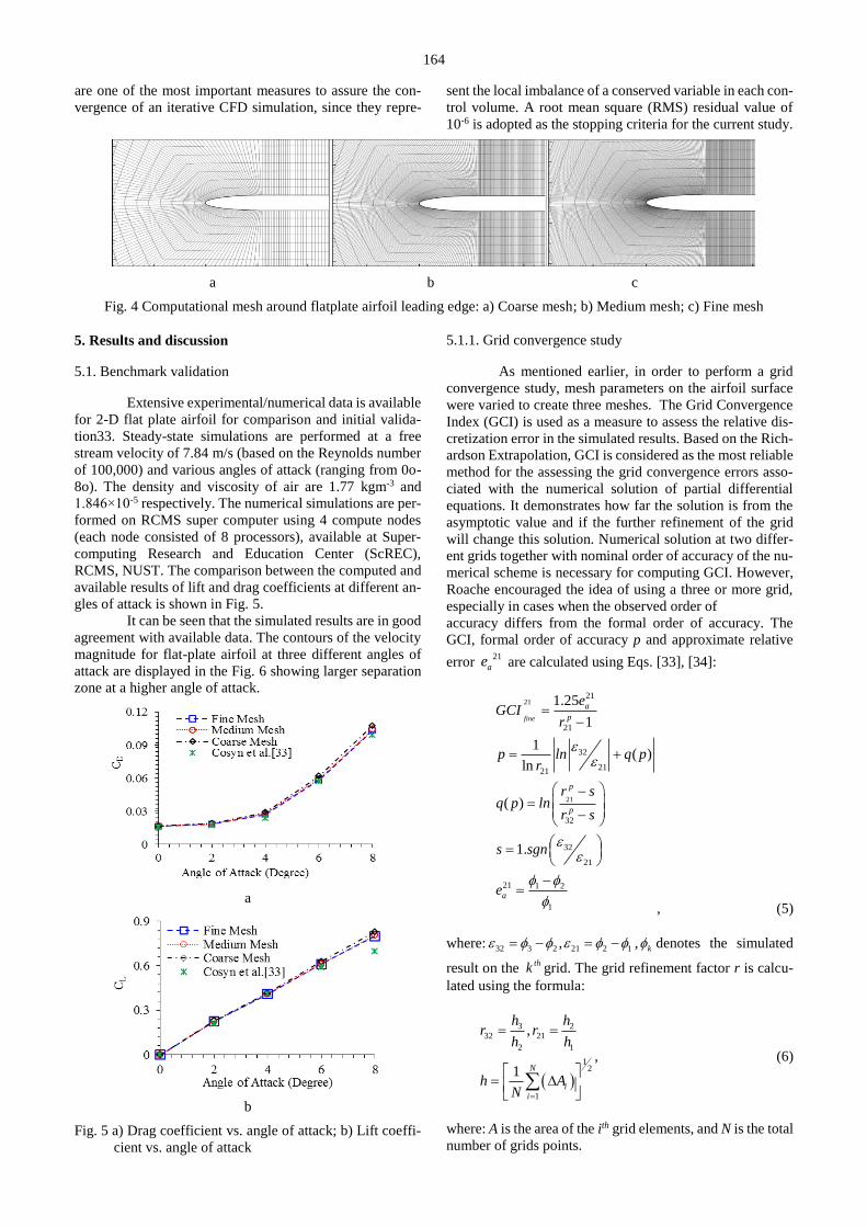
Fig. 4 Computational mesh around flatplate airfoil leading edge: a) Coarse mesh; b) Medium mesh; c) Fine mesh

5. Results and discussion

5.1. Benchmark validation

Extensive experimental/numerical data is available

for 2-D flat plate airfoil for comparison and initial valida-

tion33. Steady-state simulations are performed at a free

stream velocity of 7.84 m/s (based on the Reynolds number

of 100,000) and various angles of attack (ranging from 0o-

8o). The density and viscosity of air are 1.77 kgm-3 and

1.846×10-5 respectively. The numerical simulations are per-

formed on RCMS super computer using 4 compute nodes

(each node consisted of 8 processors), available at Super-

computing Research and Education Center (ScREC),

RCMS, NUST. The comparison between the computed and

available results of lift and drag coefficients at different an-

gles of attack is shown in Fig. 5.

It can be seen that the simulated results are in good

agreement with available data. The contours of the velocity

magnitude for flat-plate airfoil at three different angles of

attack are displayed in the Fig. 6 showing larger separation

zone at a higher angle of attack.

(a)

a

(b)

b

Fig. 5 a) Drag coefficient vs. angle of attack; b) Lift coeffi-

cient vs. angle of attack

5.1.1. Grid convergence study

As mentioned earlier, in order to perform a grid

convergence study, mesh parameters on the airfoil surface

were varied to create three meshes. The Grid Convergence

Index (GCI) is used as a measure to assess the relative dis-

cretization error in the simulated results. Based on the Rich-

ardson Extrapolation, GCI is considered as the most reliable

method for the assessing the grid convergence errors asso-

ciated with the numerical solution of partial differential

equations. It demonstrates how far the solution is from the

asymptotic value and if the further refinement of the grid

will change this solution. Numerical solution at two differ-

ent grids together with nominal order of accuracy of the nu-

merical scheme is necessary for computing GCI. However,

Roache encouraged the idea of using a three or more grid,

especially in cases when the observed order of

accuracy differs from the formal order of accuracy. The

GCI, formal order of accuracy p and approximate relative

error 21

ae are calculated using Eqs. [33], [34]:

21

21

21

21

32

2121

32

32

21

21 1 2

1

1.25

1

1( )

ln

( )

1.

fine

a

p

p

p

a

eGCI

r

p ln q pr

r sq p ln

r s

s sgn

e

, (5)

where: 32 3 2 21 2 1, , k denotes the simulated

result on the thk grid. The grid refinement factor r is calcu-

lated using the formula:

3 232 21

2 1

12

1

,

1 N

ii

h hr r

h h

h AN

, (6)

where: A is the area of the ith grid elements, and N is the total

number of grids points.

165

a

b

c

Fig. 6 Contours of velocity magnitude at different angles of

attack: a) 0°; b) 4°; c) 8°

The order of accuracy p and GCI for the simulation

results of drag coefficients on three grids are summarized in

the Tables 2. Superscripts 1, 2 and 3 represent coarse, me-

dium and fine mesh respectively. It can be observed from

Table 2 that GCI for finer grid GCI32 has relatively small

value compared to that of the coarser grid GCI21 indicating

a reduced dependency of numerical results on the cell size.

Therefore, the further grid refinement will not give a signif-

icant change in the numerical results. Since a negligible

change in the solution is expected by further mesh refine-

ment, fine mesh (mesh 3) is used for all further computa-

tions.

Table 2

Order of accuracy and grid convergence

index for drag coefficient

Angle of

attack e21 e32 p GCI21 GCI32

0° 2.01 % 1.21 % 0.31 16.27 % 14.38 %

2° 3.48 % 1.09 % 1.57 4.13 % 2.09 %

4° 4.64 % 2.02 % 0.97 10.28 % 6.89 %

6° 4.20 % 2.01 % 0.80 0.74 % 0.51 %

8° 3.70 % 0.571 % 2.87 1.69 % 0.47%

5.2. Diffuser design and optimization

In the second stage, the flat plate airfoil is used to

design a diffuser for horizontal axis hydrokinetic turbine

(parameters summarized in Table 3). Subsequently, the per-

formance of the diffuser is optimized by achieving an opti-

mum curved profile at the internal surface of the diffuser.

The Response Surface Methodology (RSM) is used as a tool

for optimization. The fluid velocity profile at the throat is

chosen as an objective function in this optimization study.

Table 3

Parameters of diffuser

Parameter Value

Diffuser length 0.38 m

Inlet diameter 0.50 m

Incoming flow velocity 2.75 m/s

The RSM procedure is carried out as follows:

1) The Bezier curve technique is used to parameterize the

airfoil geometry.

2) A 3k factorial design is used to create an experimental

table containing the combinations of design variables

representing the design space.

3) CFD simulations are performed to determine the values

of the objective function at each experimental model

4) A full quadratic regression model fitting the numerical

data is developed.

5) The optimal set of design variables producing the opti-

mum response value is determined. The schematic

flowchart is shown in Fig. 7.

Problem formulation

(Selection of design variables,

Response function)

Design of computer

experiments

Simulation of computational

experiments

Construction of regression

model

Assessment of Fit

Satisfactory

Optimization analysis

End

Yes

NO

Fig. 7 Optimization flowchart

5.2.1 Geometric parameterization of airfoil

Parameterization of the airfoil shape is an im-

portant step in the optimization process of any airfoil. In this

method, the airfoil is represented by some parameters which

control its shape. Over the past few decades, several param-

eterization techniques have been developed for this purpose.

An extensive review of these shape parameterization tech-

niques for airfoils can be found in Ref [35].

In one of the most commonly used parameteriza-

tion techniques, Bezier curves are used to fit airfoil shapes.

A Bezier parameterization of an airfoil is determined by its

166

control points. The Bezier curve of order n+1 (degree n) has

n+1 control points and it passes through the first and last

control points which are also the initial and terminal point

on the curve itself. [36]

In the present study, a 4th degree Bezier curve was

used to fit symmetric flat plate airfoil. The first and last

control points, P0 and P4 lie on the airfoil leading and trail-

ing edges respectively. The position of first point is fixed.

The remaining 4 control points are allowed to only move

vertically (keeping the abscissas fixed). The following con-

straint was also set on the y coordinate of control points to

obtain different conical diffusers and to maintain a realistic

search space.

4 3 2 1 0 .y y y y y (7)

5.2.2. Design of experiments (DOE)

Design of experiment is an important aspect of

RSM and is used to define is a sequence of experiments (nu-

merical simulation in the present case) that will be per-

formed. Since the quality of the response surface is influ-

enced by the choice of points in the design variable space, a

careful selection of this method is vital for any optimization

study. The most commonly used DOE methods include full-

factorial designs, central composite designs, Box-Behnken

designs, Latin Hypercube Design (LHD) and so on.[37]

A 3kfactorial design is used in the present case to

determine the number of required numerical measurements

of the response of interest. Here k represents the number of

varying parameters (y coordinates of 4 control points in the

present case). Out of 81 different diffuser geometries, only

15 satisfied the above mentioned condition are selected for

further analysis (shown in Fig. 8)

5.2.3. Numerical computations at the design points

CFD simulations are performed to simulate the

flow behaviour inside each diffuser. The contours of veloc-

ity magnitude inside and around three different diffusers are

displayed in Fig. 8 showing a significant increase in the flow

velocity through the turbine working section. Similarly, Ta-

ble 4 shows the value of the fluid velocity at throat of all

investigated diffuser.

Table 4

Fluid velocity at the diffuser throat

Diffuser

geometry Velocity, m/s

Diffuser

geometries Velocity, m/s

D1 2.75 D9 3.40

D2 3.57 D10 3.43

D3 3.42 D11 3.33

D4 3.319 D12 3.29

D5 3.24 D13 3.29

D6 3.59 D14 3.25

D7 3.52 D15 3.17

D8 3.46

Fig. 8 Different diffuser configurations used for CFD analysis

It can be observed that diffuser produced the max-

imum velocity augmentation of 30.55% in comparison free

stream velocity. The Contours of velocity magnitude inside

and around three different diffusers D3, D5 and D6 are dis-

played in Fig. 9.

5.2.4. Model fitting and assessment

A regression model has been developed to calcu-

late the relationship between fluid velocity at the throat and

4 design variables (control points). The estimated regression

line is:

1 2 3 43.40 3.52 2.00 1.91 1.60 .velocity y y y y (8)

For this relationship, the value of R2 (coefficient of

determination (often used as a goodness of fit for the

model)) is 96 % and adjusted R2 is 94%, which shows that

the fitted model is a good- fit. Moreover, Table 5 provides

the values of the t-test (to check the statistical significance

167

of the estimated coefficients) for the corresponding coeffi-

cients along with their standard errors. The standard errors

are low, and the corresponding p-values shows that the esti-

mated coefficients are statistically significant at 5% level of

significance. Table 6 provide the results of analysis of vari-

ance of the estimated model to check the overall adequacy

of the model. The corresponding p-value of the F-statistic

shows that the model is adequate at 5 % level of signifi-

cance. The above results show that the estimated model is

statistically validated and the predications based on this

model should have high reliability.

a

b

c

Fig. 9 Contours of velocity magnitude inside and around

different diffusers a) D3; b) D5; c) D6

5.2.5. Optimization analysis

The optimum set of input parameters producing the

optimal response value is determined using response opti-

mizer and response surface plots. Fig. 10 is showing the ef-

fect of each factor on the response or composite desirability.

Here the vertical red and horizontal blue lines represent the

current settings and response values respectively. The val-

ues of composite desirability lie between 0 and 1 which cor-

responds to the undesirable and optimal performance for the

studied factors response. So the maximum value of compo-

site desirability is showing the occurrence optimal solution.

It can be observed from Fig. 10 that the maximum velocity

that can be achieved is 3.62m/s. Hence, by using optimum

geometrical parameters for the diffuser, a velocity augmen-

tation of 31.70% can be achieved in comparison to the free

stream velocity.

Table 5

Coefficients of the estimated regression model with

standard errors and t-value

Coeffi-

cients Estimates

SE

(Coefficients) t-value

p-

value

Intercept 3.40 0.0320 06.26 0000

y2 -3.52 0.9532 -3.69 0.005

y3 -2.00 0.4764 -4.20 0.002

y4 -1.91 0.3079 -6.21 0.000

y5 1.60 0.2979 5.38 0.000

Note: SE (coefficients) is the standard error of coefficients

Table 6

Analysis of variance

Source Degrees of

freedom

Sum of

squares

Mean

squares

F-

ratio

P-

value

Re-

gres-

sion

4 0.2051 0.0513 55.15 0.000

Error 9 0.0084 0.0009

Total 13 0.2135

Fig. 10 Response optimizer for the optimum input parame-

ters

5.3. Performance analysis of optimized diffuser

The performance of optimized diffuser is analysed

using numerical actuator disc approach [38–41]. For this

purpose, first the flow around the line projection represent-

ing the actuator disc is simulated. In the model setup, the

line is assigned a fan boundary condition.

The pressure drop across the whole line is defined

using the following relation:

CurHigh

Low0.94097D

New

d = 0.94097

Maximum

Velocity

y = 3.6217

0.94097

Desirability

Composite

0.0693

0.1385

0.0

0.1059

0.0

0.0685

0.0

0.0342y3 y4 y5y2

[0.0] [0.0] [0.0002] [0.1378]

168

2,

0.5t

P Pc

U

(9)

here: is density; U is free stream velocity; Ct is thrust co-

efficient. Contours of the x component of the velocity are

displayed in Fig. 11 (a) showing a reduction in velocity fol-

lowed by the stream tube expansion due to the presence of

disk. Fig. 11 (b) shows the effect of the presence of the dif-

fuser in terms of flow augmentation at actuator disc.

a

b

Fig. 11 Contours of velocity magnitude around the a) bare

disk; b) ducted disk

It can clearly be observed that the diffuser in-

creases axial velocity, when compared to the bare actuator.

6. Conclusions

There is an increasing focus on the use of hydroki-

netic energy converters since these technologies have the

potential to offer a substantial share of the global energy

mix. The purpose of this study is the design and optimiza-

tion of diffuser for horizontal axis hydrokinetic turbine

through parametric study using computational fluid dynam-

ics technique.

After numerically validating the baseline case,

DOE is used to create fifteen different experiments and cor-

responding numerical results are analysed using surrogate

model to find the optimum geometrical parameters for the

diffuser. Later, performance of optimized diffuser is ana-

lysed using the actuator disc-RANS model. The important

conclusions reached are summarized as follows:

using a diffuser with optimum curved profile at the in-

ternal surface, maximum velocity (at the diffuser

throat) that can be achieved is 3.62 m/s.

by finding the optimum set of input parameters, a ve-

locity augmentation of 31.70 % can be attained.

The diffuser with optimum curved profile at the internal

surface showed the velocity augmentation of 1.14 times

as compared to the straight wall diffuser having almost

same area ratio [ 15D ].

The present study will be extended by performing

3D transient CFD study to analyse effect of diffuser geom-

etry on performance of an actual hydrokinetic turbine.

Moreover, turbulence in the inflow effects the performance

of diffuser augmented HAHT. The turbulence intensity (TI)

is the most commonly used parameter to describe turbulence

in marine energy applications. The impact of TI on diffuser

augmented HAHT efficiency needs to be investigated.

References

1. Pachauri, R. K.; Allen, M. R.; Barros, V.R., et al.

2014. Climate change 2014: synthesis report, Contribu-

tion of Working Groups I, II and III to the fifth assess-

ment report of the Intergovernmental Panel on Climate

Change, IPCC.

https://www.ipcc.ch/site/assets/up-

loads/2018/05/SYR_AR5_FINAL_full_wcover.pdf

2. Khan, M. J.; Iqbal, M. T.; Quaicoe, J. E. 2008. River

current energy conversion systems: Progress, prospects

and challenges, Renewable and Sustainable Energy Re-

views 12(8): 2177–2193.

https://doi.org/10.1016/j.rser.2007.04.016.

3. Khan, M. J.; Bhuyan, G.; Iqbal, M. T., et al. 2009.

Hydrokinetic energy conversion systems and assessment

of horizontal and vertical axis turbines for river and tidal

applications: Technology status review, applied energy

86(10): 1823–1835.

https://doi.org/10.1016/j.apenergy.2009.02.017.

4. Güney, M. S.; Kaygusuz, K. 2010. Hydrokinetic en-

ergy conversion systems: A technology status review.

Renewable and Sustainable Energy Reviews 14(9):

2996–3004.


5. Lago, L. I.; Ponta, F. L.; Chen, L. 2010. Advances and

trends in hydrokinetic turbine systems, Energy for Sus-

tainable Development 14(4): 287–296.

https://doi.org/10.1016/j.esd.2010.09.004.

6. Yuce, M. I.; Muratoglu, A. 2015. Hydrokinetic energy

conversion systems: A technology status review, Re-

newable and Sustainable Energy Reviews 43: 72–82.


7. Laws, N. D.; Epps, B. P. 2016. Hydrokinetic energy

conversion: Technology, research, and outlook, Renew-

able and Sustainable Energy Reviews 57: 1245–1259.

https://doi.org/10.1016/j.rser.2015.12.189

8. Fraenkel, P. L. 2002. Power from marine currents, Pro-

ceedings of the Institution of Mechanical Engineers, Part

A, Journal of Power and Energy 216(1): 1–14.

https://doi.org/10.1243%2F095765002760024782.

9. Wang, J.; Piechna, J.; Gower, B., et al. 2011. Perfor-

mance analisys of diffuser augmented composite marine

current turbine using CFD, Proceedings of the ASME 5th

International Conference on Energy Sustainability

(ES’11), 2011. Washington, DC, USA.

10. Werle, M. J.; Presz, W. M. 2008. Ducted wind/water

turbines and propellers revisited, Journal of Propulsion

and Power 24(5): 1146–1150.

https://doi.org/10.2514/1.37134.

169

11. Gaden, D. L. F.; Bibeau, E. L. 2006. Increasing Power

Density of Kinetic Turbines for Cost-effective Distrib-

uted Power Generation, POWER-GEN Renewable En-

ergy Conference, Las Vegas, USA.

http://home.cc.umanitoba.ca/~bibeauel/research/pa-

pers/2006_Gaden_powergen.pdf.

12. Kirke, B. 2006. Developments in ducted water current

turbines. Tidal paper, 1–12.

http://citeseerx.ist.psu.edu/viewdoc/down-

load?doi=10.1.1.531.3501&rep=rep1&type=pdf.

13. Gaden, D. L. F.; Bibeau, E. L. 2010. A numerical in-

vestigation into the effect of diffusers on the perfor-

mance of hydro kinetic turbines using a validated mo-

mentum source turbine model, Renewable Energy

35(6):1152–1158.

https://doi.org/10.1016/j.renene.2009.11.023.

14. Shives, M.; Crawford, C. 2010. Overall efficiency of

ducted tidal current turbines, Proc., Oceans 2010

MTS/IEEE Seattle, WA, USA, 2010, 1–6.

https://doi.org/10.1109/OCEANS.2010.5664426.

15. Sun, H.; Kyozuka, Y. 2012. Analysis of performances

of a shrouded horizontal axis tidal turbine, Proc., 2012

Oceans, Yeosu, South Korea, 2012, 1–7.

16. Lokocz, T. A. 2012. Testing of a Ducted Axial Flow

Tidal Turbine. Master’s thesis, University of Maine,

United States.

17. Khunthongjan, P.; Janyalertadun, A. 2012. A study

of diffuser angle effect on ducted water current turbine

performance using CFD, Songklanakarin Journal of Sci-

ence & Technology 34(1): 61–67.

http://rdo.psu.ac.th/sjstweb/journal/34-1/0125-3395-34-

1-61-67.pdf.

18. Mehmood, N.; Zhang, L.; Khan, J. 2012. CFD study

of NACA 0018 for diffuser design of tidal current tur-

bines, Research Journal of Applied Science, Engineer-

ing and Technology 4(21): 4552–4560.

https://pdfs.seman-

ticscholar.org/7d9e/e17bf0d592653cb956ae888f0070b

53aabca.pdf.

19. Mehmood, N.; Zhang, L.; Khan, J. 2012. Exploring

the effect of length and angle on NACA 0010 for dif-

fuser design in tidal current turbines, Applied mechanics

and materials, pp. 438–441.

https://doi.org/10.4028/www.scientific.net/AMM.201-

202.438.

20. Mehmood, N.; Zhang, L.; Khan, J. 2012. Diffuser

augmented horizontal axis tidal current turbines, Re-

search Journal of Applied Sciences, Engineering and

Technology 4(18): 3522–3532.

http://maxwellsci.com/print/rjaset/v4-3522-3532.pdf.

21. Luquet, R.; Bellevre, D.; Fréchou, D. et al. 2013. De-

sign and model testing of an optimized ducted marine

current turbine, International journal of marine energy 2:

61–80.

https://doi.org/10.1016/j.ijome.2013.05.009.

22. Shinomiya, L. D.; Aline, D.; Maria, A. et al. 2013. Nu-

merical Study of Flow around Diffusers with Different

Geometry Using CFD Applied to Hydrokinetics Tur-

bines Design, Proc., 22nd International Congress of Me-

chanical Engineering – COBEM 2013, Ribeirão Preto,

Brazil.

23. Ait-Mohammed, M.; Tarfaoui, M.; Laurens, J.M. 2014. Predictions of the hydrodynamic performance of

horizontal axis marine current turbines using a panel

method program. In: Proc., International Conference on

Renewable Energy and Power Quality (ICREPQ’14),

Cordoba, Spain.

24. Shi, W.; Wang, D.; Atlar, M. et al. 2015. Optimal de-

sign of a thin-wall diffuser for performance improve-

ment of a tidal energy system for an AUV, Ocean Engi-

neering 108: 1–9.

https://doi.org/10.1016/j.oceaneng.2015.07.064

25. Riglin, J.; Schleicher, W.C.; and Oztekin A. 2015.

Numerical analysis of a shrouded micro-hydrokinetic

turbine unit, Journal of Hydraulic Research 53(4): 525–

531.

https://doi.org/10.1080/00221686.2015.1032375.

26. Oblas, N. 2016. Design, Manufacture and Prototyping

of a Hydrokinetic Turbine Unit for River Application,

Master’s thesis, Lehigh University, Pennsylvania, USA.

27. Tampier, G.; Troncoso, C.; and Zilic, F. 2017. Nu-

merical analysis of a diffuser-augmented hydrokinetic

turbine, Ocean Engineering 145: 138–147.

https://doi.org/10.1016/j.oceaneng.2017.09.004.

28. Nunes, M. M.; Mendes, R. C. F.; Oliveira, T. F, et al.

2019. An experimental study on the diffuser-enhanced

propeller hydrokinetic turbines, Renewable Energy 133:

840–848.

https://doi.org/10.1016/j.renene.2018.10.056.

29. Versteeg, H. K.; Malalasekera, W. 2006. An Introduc-

tion to Computational Fluid Dynamics: The Finite Vol-

ume Method, 2nd ed, Pearson Education, New York.

30. Najar, N. A.; Dandotiya, D.; Najar, F. A. 2013. Com-

parative analysis of k-epsilon and spalart-allmaras tur-

bulence models for compressible flow through a conver-

gent-divergent nozzle, International Journal of Engi-

neering and Science 2: 8–17.

http://www.theijes.com/papers/v2-

i8/Part.2/B028208017.pdf.

31. Kostić, Č. 2015. Review of the Spalart-Allmaras turbu-

lence model and its modifications to three-dimensional

supersonic configurations, Scientific Technical Review

65(1): 43–49.

https://doi.org/10.5937/STR1501043K.

32. Gabriel, E. T.; Mueller, T. J. 2004. Low-aspect-ratio

wing aerodynamics at low Reynolds number, AIAA

Journal 42(5): 865–873.

https://doi.org/10.2514/1.439.

33. Celik, I. B.; Ghia, U.; Roache, P. J, et al. 2008. Proce-

dure for estimation and reporting of uncertainty due to

discretization in CFD applications, Journal of fluids En-

gineering-Transactions of the ASME 130(7): 1–4.

https://doi.org/10.1115/1.2960953.

34. Roache, P. J. 1994. Perspective: a method for uniform

reporting of grid refinement studies, Journal of Fluids

Engineering 116(3). American Society of Mechanical

Engineers: 405–413.

https://doi.org/10.1115/1.2910291.

35. Samareh, J. A. 2001. Survey of shape parameterization

techniques for high-fidelity multidisciplinary shape op-

timization, AIAA journal, 39(5): 877-884.

https://doi.org/10.2514/2.1391.

36. Derksen, R. W.; Rogalsky, T. 2010. Bezier-PARSEC:

An optimized aerofoil parameterization for design, Ad-

vances in engineering software 41(7–8): 923–930.

https://doi.org/10.1016/j.advengsoft.2010.05.002

37. Cavazzuti, M. 2013. Design of Experiments. In: Opti-

mization Methods: From Theory to Design Scientific

170

and Technological Aspects in Mechanics, Berlin, Hei-

delberg: Springer Berlin Heidelberg, pp. 13–42.

https://doi.org/10.1007/978-3-642-31187-1_2.

38. Batten, W. M. J.; Harrison, M. E.; Bahaj, A. S. 2013.

Accuracy of the actuator disc-RANS approach for pre-

dicting the performance and wake of tidal turbines, Phil-

osophical Transactions of the Royal Society A: Mathe-

matical, Physical and Engineering Sciences, 371(1985).

https://doi.org/10.1098/rsta.2012.0293.

39. Lartiga, C.; Crawford, C. 2010. Actuator disk model-

ing in support of tidal turbine rotor testing, Proc. 3rd Int.

Conf. on Ocean Energy, Bilbao, Spain, pp. 1–6.

40. Lawn, C. J. 2003. Optimization of the power output

from ducted turbines, Proceedings of the Institution of

Mechanical Engineers, Part A: Journal of Power and En-

ergy 217(1): 107–117.

https://doi.org/10.1243%2F095765003321148754.

41. Shives, M.; Crawford, C. 2012. Developing an empir-

ical model for ducted tidal turbine performance using

numerical simulation results, Proceedings of the Institu-

tion of Mechanical Engineers, Part A: Journal of Power

and Energy 226(1): 112–125.

https://doi.org/10.1177%2F0957650911417958.

W. Khalid, S. Sherbaz, A. Maqsood, Z. Hussain

DESIGN AND OPTIMIZATION OF A DIFFUSER FOR

A HORIZONTAL AXIS HYDROKINETIC TURBINE

USING COMPUTATIONAL FLUID DYNAMICS

BASED SURROGATE MODELLING

S u m m a r y

Fossil fuels have remained at the backbone of the

global energy portfolio. With the growth in the number of

factories, population, and urbanization; the burden on fossil

fuels has also been increasing. Most importantly, fossil fuels

have been causing damage to the global climate since indus-

trialization. The stated issues can only be resolved by shift-

ing to environment friendly alternate energy options. The

horizontal axis hydrokinetic turbine is considered as a viable

option for renewable energy production. The aim of this

project is the design and optimization of a diffuser for hori-

zontal axis hydrokinetic turbine using computational fluid

dynamics based surrogate modeling. The two-dimensional

flat plate airfoil is used as a benchmark and flow around the

airfoil is simulated using Ansys Fluent. Later, computa-

tional fluid dynamics analyses are carried out for baseline

diffuser generated from the flat plate airfoil. The perfor-

mance of this diffuser was optimized by achieving an opti-

mum curved profile at the internal surface of the diffuser.

The response surface methodology is used as a tool for op-

timization. A maximum velocity augmentation of 31.70% is

achieved with the optimum diffuser.

Keywords: renewable energy, hydrokinetic turbine, dif-

fuser augmentation, computational fluid dynamics, fluent.

Received June 02, 2019

Accepted April 15, 2020

Documents

Design and Optimization of a Diffuser for a Horizontal