Design and modeling of an experimental tilapia and African

i

Design and modeling of an experimental tilapia and

African catfish recirculating aquaculture system

by

Ruan Pretorius

Thesis presented in partial fulfilment of the requirements for the Degree

of

MASTER OF ENGINEERING (CHEMICAL ENGINEERING)

in the Faculty of Engineering at Stellenbosch University

Supervisor

Neill Jurgens Goosen

March 2020

ii

DECLARATION

By submitting this thesis electronically, I declare that the entirety of the work contained therein is my own, original work, that I am the sole author thereof (save to the extent explicitly otherwise stated), that reproduction and publication thereof by Stellenbosch University will not infringe any third party rights and that I have not previously in its entirety or in part submitted it for obtaining any qualification.

Date: March 2020

Copyright © 2020 Stellenbosch University All rights reserved

Stellenbosch University https://scholar.sun.ac.za

iii

PLAGIARISM DECLARATION

1. Plagiarism is the use of ideas, material and other intellectual property of another’s work andto present is as my own.

2. I agree that plagiarism is a punishable offence because it constitutes theft.

3. I also understand that direct translations are plagiarism.

4. Accordingly all quotations and contributions from any source whatsoever (including theinternet) have been cited fully. I understand that the reproduction of text without quotationmarks (even when the source is cited) is plagiarism.

5. I declare that the work contained in this assignment, except where otherwise stated, is myoriginal work and that I have not previously (in its entirety or in part) submitted it for gradingin this module/assignment or another module/assignment.

Student number: …………………………………..

Initials and surname: …………………………………..

Signature: …………………………………..

Date: …………………………………..


iv

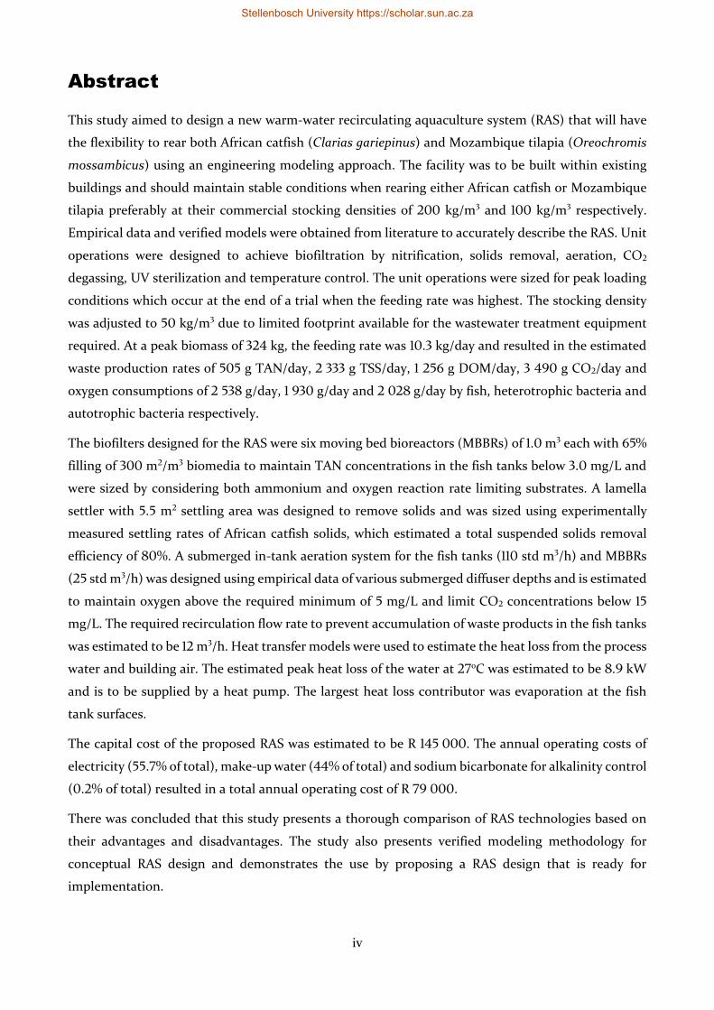
Abstract

This study aimed to design a new warm-water recirculating aquaculture system (RAS) that will have

the flexibility to rear both African catfish (Clarias gariepinus) and Mozambique tilapia (Oreochromis

mossambicus) using an engineering modeling approach. The facility was to be built within existing

buildings and should maintain stable conditions when rearing either African catfish or Mozambique

tilapia preferably at their commercial stocking densities of 200 kg/m3 and 100 kg/m3 respectively.

Empirical data and verified models were obtained from literature to accurately describe the RAS. Unit

operations were designed to achieve biofiltration by nitrification, solids removal, aeration, CO2

degassing, UV sterilization and temperature control. The unit operations were sized for peak loading

conditions which occur at the end of a trial when the feeding rate was highest. The stocking density

was adjusted to 50 kg/m3 due to limited footprint available for the wastewater treatment equipment

required. At a peak biomass of 324 kg, the feeding rate was 10.3 kg/day and resulted in the estimated

waste production rates of 505 g TAN/day, 2 333 g TSS/day, 1 256 g DOM/day, 3 490 g CO2/day and

oxygen consumptions of 2 538 g/day, 1 930 g/day and 2 028 g/day by fish, heterotrophic bacteria and

autotrophic bacteria respectively.

The biofilters designed for the RAS were six moving bed bioreactors (MBBRs) of 1.0 m3 each with 65%

filling of 300 m2/m3 biomedia to maintain TAN concentrations in the fish tanks below 3.0 mg/L and

were sized by considering both ammonium and oxygen reaction rate limiting substrates. A lamella

settler with 5.5 m2 settling area was designed to remove solids and was sized using experimentally

measured settling rates of African catfish solids, which estimated a total suspended solids removal

efficiency of 80%. A submerged in-tank aeration system for the fish tanks (110 std m3/h) and MBBRs

(25 std m3/h) was designed using empirical data of various submerged diffuser depths and is estimated

to maintain oxygen above the required minimum of 5 mg/L and limit CO2 concentrations below 15

mg/L. The required recirculation flow rate to prevent accumulation of waste products in the fish tanks

was estimated to be 12 m3/h. Heat transfer models were used to estimate the heat loss from the process

water and building air. The estimated peak heat loss of the water at 27oC was estimated to be 8.9 kW

and is to be supplied by a heat pump. The largest heat loss contributor was evaporation at the fish

tank surfaces.

The capital cost of the proposed RAS was estimated to be R 145 000. The annual operating costs of

electricity (55.7% of total), make-up water (44% of total) and sodium bicarbonate for alkalinity control

(0.2% of total) resulted in a total annual operating cost of R 79 000.

There was concluded that this study presents a thorough comparison of RAS technologies based on

their advantages and disadvantages. The study also presents verified modeling methodology for

conceptual RAS design and demonstrates the use by proposing a RAS design that is ready for

implementation.


v

Opsomming

Hierdie studie het beoog om ’n nuwe warmwater hersirkuleringsakwakultuurstelsel (RAS) te ontwerp

wat die buigbaarheid het om beide Afrika-baber (Clarias gariepinus) en Mosambiekse kurper

(Oreochromis mossambicus) te kweek deur ’n ingenieursmodelleringsbenadering te gebruik. Die

fasiliteit moes gebou word binne bestaande geboue en moet stabiele kondisies behou wanneer óf

Afrika-baber óf Mosambiekse kurper verkieslik by hul kommersiële voorraaddigthede van 200 kg/m3

en 100 kg/m3 onderskeidelik gekweek word. Empiriese data en bevestigde modelle is verkry uit

literatuur om die RAS akkuraat te beskryf. Bedryfseenhede is ontwerp om biofiltrasie deur nitrifikasie,

verwydering van vaste stof, belugting, CO2-ontgassing, UV-sterilisasie en temperatuur kontrole te

bereik. Die bedryfseenhede is geskaal vir kondisies van spitslading wat plaasvind teen die einde van ’n

toets as die voertempo op sy hoogste was. Die voorraaddigtheid is aangepas na 50 kg/m3 as gevolg

van beperkte staanoppervlakte beskikbaar vir die afvalwaterbehandeling se toerusting wat benodig

word. By spitsbiomassa van 324 kg, was die voertempo 10.3 kg/dag en het die beraamde

afvalproduksietempo’s van 505 g TAN/dag, 2 333g TSS/dag, 1 256 g DOM/dag, 3 490 g CO2/dag en

suurstofgebruik 2 538 g/dag, 1 930g/dag en 2 028 g/dag deur visse, heterotrofiese bakterieë en

outotrofiese bakterieë onderskeidelik tot gevolg gehad. Die biofilters ontwerp vir die RAS was ses

bewegende bed-bioreaktors (MBBR) van 1.0 m3 elk met 65% vulling van 300 m2/m3 biomedia om TAN-

konsentrasie in die vistenks onder 3.0 mg/L te behou en is geskaal deur beperkende-substrate van

beide ammonium- en suurstof-reaksietempo’s in ag te neem. ’n Lamella besinker met 5.5 m2

besinkingsarea is ontwerp om vaste stowwe te verwyder en is geskaal deur ekperimenteel-gemete

besinkingstempo’s van Afrika-baber se vaste stowwe te gebruik, wat ’n totaal

verwyderingsdoeltreffendheid van hangende vaste stof van 80% beraam het. ’n Onderdompelde

binne-tenk belugtingsisteem vir die vistenks (110 std m3/h) en MBBRe (25 std m3/h) is ontwerp deur

empiriese data van verskeie onderdompelde verspreier dieptes te gebruik en is beraam om suurstof bo

die vereiste minimum van 5 mg/L te handhaaf en CO2-konsentrasies onder 15 mg/L te beperk. Die

vereiste sirkulasie vloeitempo om akkumulasie van afvalprodukte in die vistenks te verhoed, is beraam

om 12 m3/h te wees. Hitte-oordragmodelle is gebruik om die hitteverlies van die proseswater en

geboulug te beraam. Die beraamde spitshittteverlies van die water by 27°C is beraam om 8.9 kW te

wees en is voorsien deur ’n hittepomp. Die grootste bydraer van hitteverlies was verdamping by die

vistenkoppervlak.

Die kapitaalkoste van die voorgestelde RAS is beraam om R 145 000 te wees. Die jaarlikse koste van

elektrisiteit (55.7% van totaal), aanvullingswater (44% van totaal) en koeksoda vir alkaliniteitbeheer

(0.2% van totaal) het ’n totale jaarlikse bedryfskoste van R 79 000 tot gevolg gehad.

Daar is tot die gevolg gekom dat hierdie studie ’n deeglike vergelyking van RAS-tegnologieë lewer

gebaseer op hul voordele en nadele. Die studie het modellering metodologie vir konsepsuele RAS-

ontwerp bewys en stel die gebruik daarvan voor deur ’n RAS-ontwerp wat reg is vir implementasie.


vi

Acknowledgements

Firstly, I would like to acknowledge the excellent support of my supervisor, Dr. Neill Goosen. Without

his expert guidance, none of this work would have been possible.

My appreciation goes to the Department of Process Engineering at Stellenbosch University for the

funding that made this study a reality.

I would like to acknowledge my dear friend Janus Louw for the many stimulating conversations that

often helped me gain insight on details I was missing at the time.

Last, but certainly not least, I would like to the thank my parents, Johan and Francis Pretorius, for

their continued loving support throughout my studies and for that I am eternally grateful.


vii

Dedication

I dedicate this thesis to my loving wife and soul mate, Beth Pretorius. This undertaking would surely

have failed without her undying support by picking me up when I’m down and spurring me on. Thank

you for giving me the strength and showing me that sometimes it is worth it to just have a bit of faith.


viii

Nomenclature - List of abbreviations

ADG Average daily gain

AGR Absolute growth rate

ASM Activated sludge model

BOD Biochemical oxygen demand

BOD5 5-day biochemical oxygen demand

BP Barometric pressure

BW Body weight

CBOD Carbonaceous biochemical oxygen demand

COD Chemical oxygen demand

CSTR Continuous stirred-tank reactor

DE Diatomaceous earth

DO Dissolved oxygen

DOM Dissolved organic matter

DP Differential pressure

FBB Floating bead biofilter

FCR Feed conversion ratio

FSB Fluidized sand biofilter

HDPE High-density polyethylene

HSL Hydraulic surface loading rate

LLDPE Linear low-density polyethylene

MBBR Moving bed bioreactor

NR Nitrogen retention

PFD Process flow diagram

P&ID Piping and instrumentation diagram

PM Porous media

POM Particulate organic matter

PVC Polyvinyl chloride

RAS Recirculating aquaculture system

RBC Rotating biological contactor

SG Specific gravity

SGR Specific growth rate

STP Standard temperature and pressure

TAN Total ammonia nitrogen

TDS Total dissolved solids

TGC Temperature growth coefficient

TGP Total dissolved gas pressure

TMY Typical meteorological year

TSS Total suspended solids

UV Ultraviolet

VBGF Von Bertalanffy growth function

WWT Wastewater treatment

ZAR South African Rand


ix

Nomenclature - List of symbols

Symbol Units Description

𝐴 𝑚2 Area

𝐴𝑏𝑖𝑜𝑓𝑖𝑙𝑚 𝑚2 Biofilm area

𝐴𝑐 𝑚2 Cross-sectional area

𝐴𝑠 𝑚2 Heat transfer surface area

𝐴𝑠𝑒𝑡𝑡𝑙𝑒 𝑚2 Horizontally projected settling area

𝐴𝐺𝑅 𝑔 𝑑𝑎𝑦⁄ Absolute growth rate

𝑎1 𝑔0.5 (𝑚0.5 ∙ 𝑑𝑎𝑦)⁄ Trickling filter model parameter

𝑎2 𝑔 (𝑚2 ∙ 𝑑𝑎𝑦)⁄ Trickling filter model parameter

𝑎3 𝑔 (𝑚2 ∙ 𝑑𝑎𝑦)⁄ Trickling filter model parameter

𝛼 Dimensionless Ratio of oxygen transfer coefficients at field and clean water conditions

𝛽 Dimensionless Ratio of oxygen saturation concentration at field and clean water conditions

𝐵 1 𝐾⁄ Coefficient of volume expansion

𝐵𝑂𝐷5,𝑝𝑟𝑜𝑑 𝑔 𝐵𝑂𝐷5 𝑑𝑎𝑦⁄ Daily BOD5 production

𝑏 Dimensionless Allometric exponent

𝐵𝑃 𝑚𝑚𝐻𝑔 Local barometric pressure

𝑐𝑝 𝐽 (𝑘𝑔 ∙ 𝐾⁄ ) Specific heat capacity

𝑐𝑝,𝑤 𝐽 (𝑘𝑔 ∙ 𝐾⁄ ) Specific heat capacity of water

𝐶 𝑚𝑔 𝐿⁄ Concentration

𝐶𝑁,𝑝𝑟𝑜𝑡𝑒𝑖𝑛 𝑔 𝑁 𝑔 𝑝𝑟𝑜𝑡𝑒𝑖𝑛⁄ Nitrogen content of protein

𝐶𝑁𝐻3−𝑁 𝑚𝑔 𝐿⁄ Un-ionized ammonia concentration

𝐶𝑁𝑂3−𝑁,𝑚𝑎𝑥 𝑚𝑔 𝐿⁄ Maximum allowable nitrate concentration

𝐶𝐶𝑂2 𝑚𝑔 𝐿⁄ Dissolved carbon dioxide concentration

𝐶𝐶𝑂2

𝑠𝑎𝑡 𝑚𝑔 𝐿⁄ Saturation concentration of carbon dioxide in water

𝐶𝑂2 𝑚𝑔 𝐿⁄ Dissolved oxygen concentration

𝐶𝑂2

∗ 𝑚𝑔 𝐿⁄ Reaction order transition oxygen concentration

𝐶𝑂2

𝑠𝑎𝑡 𝑚𝑔 𝐿⁄ Saturation concentration of oxygen in water

(𝐶𝑂2

𝑠𝑎𝑡)𝑒𝑓𝑓

𝑚𝑔 𝐿⁄ Mean effective dissolved oxygen saturation concentration

(𝐶𝑂2

𝑠𝑎𝑡)𝐶𝑊

𝑚𝑔 𝐿⁄ Oxygen saturation concentration under clean conditions

(𝐶𝑂2

𝑠𝑎𝑡)𝐹𝑊

𝑚𝑔 𝐿⁄ Oxygen saturation concentration under field conditions

𝐶𝑝𝑟𝑜𝑡𝑒𝑖𝑛 𝑔 𝑝𝑟𝑜𝑡𝑒𝑖𝑛 𝑔 𝑓𝑒𝑒𝑑⁄ Feed protein content

𝐶𝑇𝐴𝑁 𝑚𝑔 𝐿⁄ Total ammonia nitrogen concentration

𝐶𝑇𝐴𝑁∗ 𝑚𝑔 𝐿⁄ Reaction order transition TAN concentration

𝐷 𝑚 Diameter

𝐷ℎ 𝑚 Hydraulic diameter of the geometry

𝐷𝑝 𝑚 Particle diameter

𝐷𝑖𝑛𝑛𝑒𝑟 𝑚 Inner pipe diameter

𝐷𝑜𝑢𝑡𝑒𝑟 𝑚 Outer pipe diameter

𝐷𝑝𝑖𝑝𝑒 𝑚 Pipe diameter

𝐷𝑃 𝑚𝑚𝐻𝑔 Difference between TGP and BP

𝜀 Dimensionless Emissivity

𝜉 𝑚 Pipe surface roughness

𝐹 𝑚𝑚𝐻𝑔 (𝑚𝑔 𝐿⁄ )⁄ Gas tension factor

𝑓 Dimensionless Darcy friction factor

𝐺𝑟𝐿 Dimensionless Grashof number


x

𝑔 𝑚 𝑠2⁄ Gravitational acceleration

{𝐻+} Dimensionless Activity of hydrogen ions

𝐻𝑆𝐿 𝑚3 (𝑚2 ∙ 𝑑𝑎𝑦)⁄ Hydraulic surface loading rate

𝐻 𝑊 Heat transfer rate

𝐻𝑚𝑎𝑘𝑒𝑢𝑝 𝑊 Heat transfer rate due to make-up water addition

ℎ 𝑚 Height

ℎ𝑑𝑖𝑓𝑓𝑢𝑠𝑒𝑟 𝑚 Diffuser depth

ℎ𝐿 𝑚 Head loss

ℎ𝑡𝑓 𝑚 Distance from the top of the trickling filter

𝐾𝐿𝑎𝐶𝑂2 1 𝑑𝑎𝑦⁄ Overall carbon dioxide mass transfer coefficient

𝐾𝐿𝑎𝑂2 1 𝑑𝑎𝑦⁄ Overall oxygen mass transfer coefficient

(𝐾𝐿𝑎𝑂2)

𝐶𝑊 1 𝑑𝑎𝑦⁄ Overall oxygen mass transfer coefficient under clean water conditions

(𝐾𝐿𝑎𝑂2)

𝐹𝑊 1 𝑑𝑎𝑦⁄ Overall oxygen mass transfer coefficient under field conditions

𝑘𝑑𝑒𝑎𝑡ℎ 1 𝑑𝑎𝑦⁄ Mortality rate

𝑘𝑀𝐵𝐵𝑅 𝑔1−𝑛𝑟𝑚3𝑛𝑟−1 𝑑𝑎𝑦⁄ MBBR reaction rate constant

𝑘𝑉𝐵𝐺𝐹 1 𝑑𝑎𝑦⁄ Von Bertalanffy growth coefficient

𝜅 𝑊 (𝑚 ∙ 𝐾)⁄ Thermal conductivity

𝜅𝑎𝑖𝑟 𝑊 (𝑚 ∙ 𝐾)⁄ Thermal conductivity of air

𝜅𝑤𝑎𝑙𝑙 𝑊 (𝑚 ∙ 𝐾)⁄ Thermal conductivity of wall material

𝜆𝑤 𝑘𝐽 𝑘𝑔⁄ Latent heat of vaporization of water

𝑙 𝑚 Fish length

𝐿𝑐 𝑚 Characteristic length of the geometry

𝐿𝑝𝑖𝑝𝑒 𝑚 Pipe length

𝐿𝑝𝑙𝑎𝑡𝑒 𝑙𝑒𝑛𝑔𝑡ℎ 𝑚 Lamella settler plate length

𝐿𝑝𝑙𝑎𝑡𝑒 𝑤𝑖𝑑𝑡ℎ 𝑚 Lamella settler plate width

𝐿𝑤𝑎𝑙𝑙 𝑚 Wall thickness

𝑚 𝑔 𝑑𝑎𝑦⁄ Mass flow rate

𝑚𝑎𝑐𝑐 𝑔 𝑑𝑎𝑦⁄ Mass accumulation rate

𝑚𝐶𝑂2 𝑔 𝑑𝑎𝑦⁄ Mass transfer rate of carbon dioxide into the water

(𝑚𝑐𝑜𝑛𝑠)𝐶𝑂2 𝑔 𝑑𝑎𝑦⁄ Carbon dioxide removed by aeration

(𝑚𝑐𝑜𝑛𝑠)𝑂2 𝑔 𝑑𝑎𝑦⁄ Oxygen consumed by fish metabolism

𝑚𝑓𝑒𝑒𝑑 𝑔 𝑓𝑒𝑒𝑑 𝑑𝑎𝑦⁄ Feeding rate

𝑚𝑂2 𝑔 𝑑𝑎𝑦⁄ Oxygen mass transfer rate

(𝑚𝑝𝑟𝑜𝑑)𝐶𝑂2

𝑔 𝑑𝑎𝑦⁄ Carbon dioxide excreted by fish

(𝑚𝑝𝑟𝑜𝑑)𝑂2

𝑔 𝑑𝑎𝑦⁄ Oxygen added by aeration

(𝑚𝑝𝑟𝑜𝑑)𝑇𝐴𝑁

𝑔 𝑑𝑎𝑦⁄ Total ammonia nitrogen produced by feeding

(𝑚𝑝𝑟𝑜𝑑)𝑇𝑆𝑆

𝑔 𝑑𝑎𝑦⁄ Total suspended solids produced by feeding

𝑚𝑟𝑒𝑐𝑖𝑟𝑐,𝑖𝑛 𝑔 𝑑𝑎𝑦⁄ Influent mass flow rate

𝑚𝑟𝑒𝑐𝑖𝑟𝑐,𝑜𝑢𝑡 𝑔 𝑑𝑎𝑦⁄ Effluent mass flow rate

𝜇 𝑃𝑎 ∙ 𝑠 Dynamic viscosity

𝜇𝑤 𝑃𝑎 ∙ 𝑠 Dynamic viscosity of water

Φ degrees Lamella settler plate inclination with the horizontal plane

𝜑 Dimensionless Submerged diffuser model parameter

𝜂𝑎 Dimensionless Absorption efficiency of aeration

𝜂𝑏𝑙𝑜𝑤𝑒𝑟 Dimensionless Blower efficiency

𝑁𝐹𝑊 𝑙𝑏 𝑂2 (ℎ𝑝 ∙ ℎ)⁄ Oxygen transfer efficiency at field conditions

𝑁𝑠𝑡𝑑 𝑙𝑏 𝑂2 (ℎ𝑝 ∙ ℎ)⁄ Oxygen transfer efficiency at standard conditions

𝑁𝑢 Dimensionless Nusselt number

𝑁𝑅 𝑔 𝑁 𝑟𝑒𝑡𝑎𝑖𝑛𝑒𝑑 𝑔 𝑁 𝑖𝑛𝑡𝑎𝑘𝑒⁄ Nitrogen retention in the fish


xi

𝑛𝑖 N/A Initial number of fish

𝑛𝑡 N/A Number of fish at time 𝑡

𝑛𝑟 Dimensionless Reaction order

𝑃 𝑃𝑎 Pressure

𝑃𝑟 Dimensionless Relative pressure

𝑃𝑏𝑙𝑜𝑤𝑒𝑟 ℎ𝑝 or 𝑘𝑊 Blower input power

𝑃𝑇𝐴𝑁 𝑔 𝑁 𝑑𝑎𝑦⁄ Total ammonia-nitrogen added to water

𝑝𝐾𝑎 Dimensionless Acid dissociation constant

𝑝𝑛 Dimensionless Percentage of population that died in mortality data

𝜌 𝑘𝑔 𝑚3⁄ Density

𝜌𝑝 𝑘𝑔 𝑚3⁄ Particle density

𝜌𝑤 𝑘𝑔 𝑚3⁄ Density of water

𝜌𝑠𝑡𝑜𝑐𝑘𝑖𝑛𝑔 𝑘𝑔 𝑚3⁄ Peak fish stocking density

𝑄𝑎𝑖𝑟 𝑚3/ℎ Air volumetric flow rate at STP of 0oC and 101 325 Pa

𝑄𝑚𝑎𝑘𝑒𝑢𝑝 𝑚3 𝑑𝑎𝑦⁄ Make-up water volumetric flow rate

𝑄𝑟𝑒𝑐𝑖𝑟𝑐 𝑚3 𝑑𝑎𝑦⁄ Recirculation flow rate

𝑅𝑒 Dimensionless Reynolds number

Λ 𝐾 𝑊⁄ Thermal resistance

Λ𝑐𝑜𝑛𝑑 𝐾 𝑊⁄ Thermal resistance against heat transfer by conduction

Λ𝑐𝑜𝑛𝑑,𝑝𝑖𝑝𝑒 𝐾 𝑊⁄ Thermal resistance against heat transfer by conduction through a circular pipe wall

Λ𝑐𝑜𝑛𝑣 𝐾 𝑊⁄ Thermal resistance against heat transfer by convective

Λ𝑟𝑎𝑑 𝐾 𝑊⁄ Thermal resistance against heat transfer by radiation

ℋ 𝑔 𝐻2𝑂 𝑚3⁄ Absolute humidity

ℛ Dimensionless Relative humidity

𝑟𝑇𝐴𝑁 𝑔 (𝑚2 ∙ 𝑑𝑎𝑦)⁄ Nitrification reaction rate

𝑟𝑇𝐴𝑁,𝑚𝑎𝑥 𝑔 (𝑚2 ∙ 𝑑𝑎𝑦)⁄ Intrinsic nitrification reaction rate

𝑆𝐺𝑅 %𝐵𝑊 𝑑𝑎𝑦⁄ Specific growth rate

𝜃 Dimensionless Temperature activity coefficient

𝑇 𝐾 or ℃ Temperature

𝑇𝑎𝑖𝑟 𝐾 or ℃ Air temperature

𝑇𝑓𝑖𝑙𝑚 𝐾 or ℃ Air film temperature

𝑇𝑚𝑎𝑘𝑒𝑢𝑝 𝐾 or ℃ Make-up water temperature

𝑇𝑃𝑊 𝐾 or ℃ Process water temperature

𝑇𝑠 𝐾 or ℃ Surface temperature

𝑇∞ 𝐾 or ℃ Air temperature sufficiently far away from the surface

𝑇𝐺𝐶 𝑔1 𝑏⁄ (℃ ∙ 𝑑𝑎𝑦)⁄ Temperature growth coefficient

𝑇𝐺𝑃 𝑚𝑚𝐻𝑔 Total dissolved gas pressure

𝑡 𝑑𝑎𝑦𝑠 Production time

𝑡𝑝 𝑑𝑎𝑦𝑠 Length of production cycle of mortality data

𝜏 𝑚𝑚𝐻𝑔 Gas tension

𝑢 𝑚 𝑠⁄ Velocity

𝑢𝑎𝑣𝑔 𝑚 𝑠⁄ Average flow velocity

𝑢𝑜 𝑚 𝑠⁄ Overflow rate

𝑢𝑠 𝑚 𝑠⁄ Settling velocity

𝑉 𝑚3 Volume

𝑣 𝑚2 𝑠⁄ Kinematic viscosity

𝑣𝑤 𝑚2 𝑠⁄ Kinematic viscosity of water

𝑤𝑖𝑛𝑓 𝑔 Asymptotic weight


xii

𝑤𝑖 𝑔 Initial fish body weight

𝑤𝑡 𝑔 Fish body weight at time 𝑡

𝜓 𝑊 (𝑚2 ∙ 𝐾)⁄ Heat transfer coefficient

𝜓𝑐𝑜𝑛𝑣 𝑊 (𝑚2 ∙ 𝐾)⁄ Convection heat transfer coefficient

𝜓𝑟𝑎𝑑 𝑊 (𝑚2 ∙ 𝐾)⁄ Radiation heat transfer coefficient

𝑥 𝑔 𝐻2𝑂 𝑘𝑔 𝑑𝑟𝑦 𝑎𝑖𝑟⁄ Mixing ratio

𝑦 Dimensionless Percentage reduction in nitrification rate relative to pH 8

𝑍 𝑔 𝐵𝑂𝐷5 (𝑚2 ∙ 𝑑𝑎𝑦)⁄ Organic loading

𝜁 𝑚 Altitude of the site


xiii

Table of contents

Chapter 1. Introduction to recirculating aquaculture systems (RAS) ................................................. 1

1.1 Introduction ................................................................................................................................ 1

1.2 Recirculating aquaculture systems (RASs) ................................................................................ 2

1.3 Motivation for the study .............................................................................................................3

1.4 Objectives and scope of the study ............................................................................................. 4

1.5 Structure of the thesis ................................................................................................................ 5

Chapter 2. Literature survey of RAS technology ................................................................................. 6

2.1 Water quality parameters .......................................................................................................... 6

2.2 Biofiltration ............................................................................................................................... 15

2.3 Solids removal .......................................................................................................................... 20

2.4 Aeration and oxygenation ........................................................................................................ 23

2.5 Carbon dioxide degassing ........................................................................................................ 24

2.6 Disinfection .............................................................................................................................. 24

2.7 Water and air heating .............................................................................................................. 25

2.8 Waste management ................................................................................................................. 25

2.9 Conclusions .............................................................................................................................. 25

Chapter 3. Steady state RAS modeling methods ............................................................................... 26

3.1 Introduction ............................................................................................................................. 26

3.2 Fish growth, mortality and feeding ......................................................................................... 27

3.3 Waste production models ........................................................................................................ 34

3.4 Biofiltration modeling .............................................................................................................. 38

3.5 Solids removal modeling .......................................................................................................... 47

3.6 Aeration and degassing models ............................................................................................... 52

3.7 Pipe flow pressure drop ........................................................................................................... 56

3.8 Fish tank mass balances ........................................................................................................... 57

3.9 Water and air heat transfer models ......................................................................................... 59

Chapter 4. Conceptual design results ................................................................................................ 70

4.1 Design basis .............................................................................................................................. 72

4.2 Initial site layout ....................................................................................................................... 79

4.3 Fish tank design........................................................................................................................ 80


xiv

4.4 Solids removal design ............................................................................................................... 82

4.5 Biological filtration design ....................................................................................................... 89

4.6 Aeration design ........................................................................................................................ 97

4.7 Water and air distribution design .......................................................................................... 102

4.8 Temperature regulation design .............................................................................................. 105

4.9 Disinfection design.................................................................................................................. 107

4.10 Water quality measurements .................................................................................................. 108

Chapter 5. System design proposal ................................................................................................... 109

5.1 Required equipment and costs ............................................................................................... 109

5.2 Drawings of proposed facility ................................................................................................... 111

5.3 RAS dimensioning heuristics ................................................................................................... 112

5.4 RAS management plan ............................................................................................................. 112

5.5 Conclusions .............................................................................................................................. 117

5.6 Recommendations for process optimization .......................................................................... 118

References…………………………………………………………………………………………………………………………………………120

: Design variables ............................................................................................................. 129

: Equipment data sheets .................................................................................................. 132

Lamella settler data sheet ....................................................................................................... 132

Moving bed bioreactor data sheet .......................................................................................... 132

Blower data sheet .................................................................................................................... 133

Heat pump data sheet ............................................................................................................. 133

Pump and blower performance curves ................................................................................... 134

: Piping and instrumentation diagrams (P&IDs) ............................................................ 136

: Bill of quantities ............................................................................................................. 138

: Carbonate reaction equilibria ....................................................................................... 140

: Gas properties ................................................................................................................. 141

Nitrogen and oxygen properties .............................................................................................. 141

Air and water vapour properties .............................................................................................. 141

: Lamella settler design .................................................................................................... 143

: MBBR oxygen concentration optimization .................................................................. 145

: Air distribution system sizing ....................................................................................... 147


xv

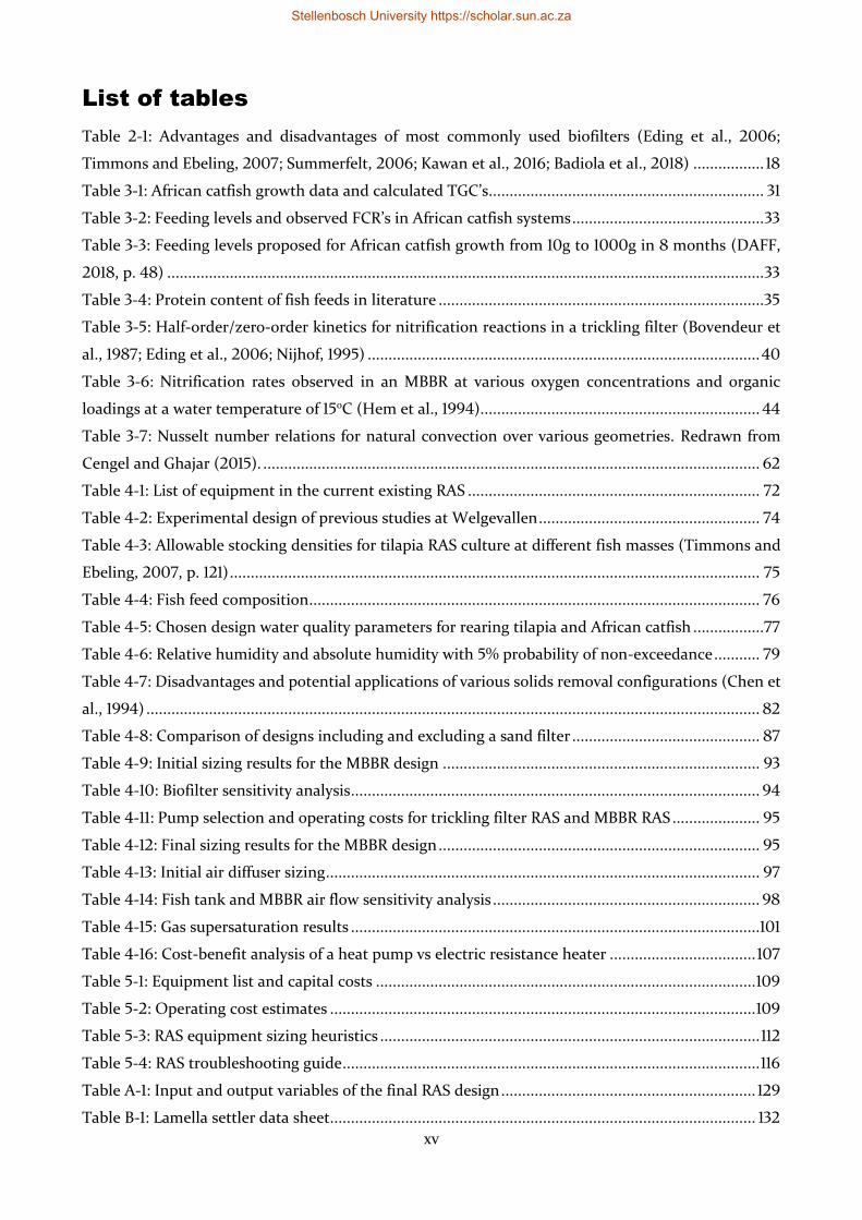
List of tables

Table 2-1: Advantages and disadvantages of most commonly used biofilters (Eding et al., 2006;

Timmons and Ebeling, 2007; Summerfelt, 2006; Kawan et al., 2016; Badiola et al., 2018) ................. 18

Table 3-1: African catfish growth data and calculated TGC’s.................................................................. 31

Table 3-2: Feeding levels and observed FCR’s in African catfish systems .............................................. 33

Table 3-3: Feeding levels proposed for African catfish growth from 10g to 1000g in 8 months (DAFF,

2018, p. 48) ............................................................................................................................................... 33

Table 3-4: Protein content of fish feeds in literature .............................................................................. 35

Table 3-5: Half-order/zero-order kinetics for nitrification reactions in a trickling filter (Bovendeur et

al., 1987; Eding et al., 2006; Nijhof, 1995) .............................................................................................. 40

Table 3-6: Nitrification rates observed in an MBBR at various oxygen concentrations and organic

loadings at a water temperature of 15oC (Hem et al., 1994) ................................................................... 44

Table 3-7: Nusselt number relations for natural convection over various geometries. Redrawn from

Cengel and Ghajar (2015). ....................................................................................................................... 62

Table 4-1: List of equipment in the current existing RAS ...................................................................... 72

Table 4-2: Experimental design of previous studies at Welgevallen ..................................................... 74

Table 4-3: Allowable stocking densities for tilapia RAS culture at different fish masses (Timmons and

Ebeling, 2007, p. 121) ............................................................................................................................... 75

Table 4-4: Fish feed composition ............................................................................................................ 76

Table 4-5: Chosen design water quality parameters for rearing tilapia and African catfish .................77

Table 4-6: Relative humidity and absolute humidity with 5% probability of non-exceedance ........... 79

Table 4-7: Disadvantages and potential applications of various solids removal configurations (Chen et

al., 1994) ................................................................................................................................................... 82

Table 4-8: Comparison of designs including and excluding a sand filter ............................................. 87

Table 4-9: Initial sizing results for the MBBR design ............................................................................ 93

Table 4-10: Biofilter sensitivity analysis .................................................................................................. 94

Table 4-11: Pump selection and operating costs for trickling filter RAS and MBBR RAS ..................... 95

Table 4-12: Final sizing results for the MBBR design ............................................................................. 95

Table 4-13: Initial air diffuser sizing ........................................................................................................ 97

Table 4-14: Fish tank and MBBR air flow sensitivity analysis ................................................................ 98

Table 4-15: Gas supersaturation results ..................................................................................................101

Table 4-16: Cost-benefit analysis of a heat pump vs electric resistance heater ................................... 107

Table 5-1: Equipment list and capital costs ........................................................................................... 109

Table 5-2: Operating cost estimates ...................................................................................................... 109

Table 5-3: RAS equipment sizing heuristics ........................................................................................... 112

Table 5-4: RAS troubleshooting guide .................................................................................................... 116

Table A-1: Input and output variables of the final RAS design ............................................................. 129

Table B-1: Lamella settler data sheet...................................................................................................... 132


xvi

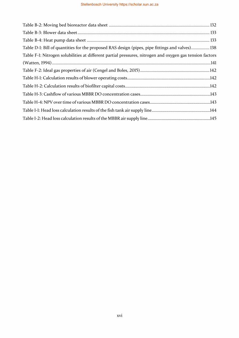
Table B-2: Moving bed bioreactor data sheet ....................................................................................... 132

Table B-3: Blower data sheet .................................................................................................................. 133

Table B-4: Heat pump data sheet .......................................................................................................... 133

Table D-1: Bill of quantities for the proposed RAS design (pipes, pipe fittings and valves)................ 138

Table F-1: Nitrogen solubilities at different partial pressures, nitrogen and oxygen gas tension factors

(Watten, 1994) ......................................................................................................................................... 141

Table F-2: Ideal gas properties of air (Cengel and Boles, 2015) ............................................................ 142

Table H-1: Calculation results of blower operating costs……………………………………………………………….…..142

Table H-2: Calculation results of biofilter capital costs……………………………………………………………………..142

Table H-3: Cashflow of various MBBR DO concentration cases…………………………………………………………143

Table H-4: NPV over time of various MBBR DO concentration cases…………………………………………………143

Table I-1: Head loss calculation results of the fish tank air supply line……………………………………………….144

Table I-2: Head loss calculation results of the MBBR air supply line……………………………………………..……145


xvii

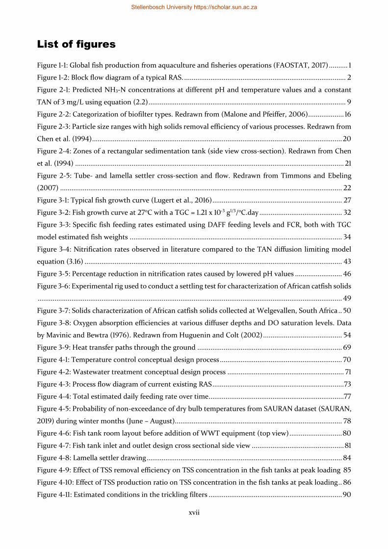
List of figures

Figure 1-1: Global fish production from aquaculture and fisheries operations (FAOSTAT, 2017) .......... 1

Figure 1-2: Block flow diagram of a typical RAS. ...................................................................................... 2

Figure 2-1: Predicted NH3-N concentrations at different pH and temperature values and a constant

TAN of 3 mg/L using equation (2.2) ......................................................................................................... 9

Figure 2-2: Categorization of biofilter types. Redrawn from (Malone and Pfeiffer, 2006) ................... 16

Figure 2-3: Particle size ranges with high solids removal efficiency of various processes. Redrawn from

Chen et al. (1994) ..................................................................................................................................... 20

Figure 2-4: Zones of a rectangular sedimentation tank (side view cross-section). Redrawn from Chen

et al. (1994) ............................................................................................................................................... 21

Figure 2-5: Tube- and lamella settler cross-section and flow. Redrawn from Timmons and Ebeling

(2007) ...................................................................................................................................................... 22

Figure 3-1: Typical fish growth curve (Lugert et al., 2016) ..................................................................... 27

Figure 3-2: Fish growth curve at 27oC with a TGC = 1.21 x 10-3 g1/3/oC.day ............................................ 32

Figure 3-3: Specific fish feeding rates estimated using DAFF feeding levels and FCR, both with TGC

model estimated fish weights ................................................................................................................. 34

Figure 3-4: Nitrification rates observed in literature compared to the TAN diffusion limiting model

equation (3.16) ......................................................................................................................................... 43

Figure 3-5: Percentage reduction in nitrification rates caused by lowered pH values ......................... 46

Figure 3-6: Experimental rig used to conduct a settling test for characterization of African catfish solids

.................................................................................................................................................................. 49

Figure 3-7: Solids characterization of African catfish solids collected at Welgevallen, South Africa .. 50

Figure 3-8: Oxygen absorption efficiencies at various diffuser depths and DO saturation levels. Data

by Mavinic and Bewtra (1976). Redrawn from Huguenin and Colt (2002) .......................................... 54

Figure 3-9: Heat transfer paths through the ground ............................................................................. 69

Figure 4-1: Temperature control conceptual design process ................................................................. 70

Figure 4-2: Wastewater treatment conceptual design process .............................................................. 71

Figure 4-3: Process flow diagram of current existing RAS ...................................................................... 73

Figure 4-4: Total estimated daily feeding rate over time ........................................................................77

Figure 4-5: Probability of non-exceedance of dry bulb temperatures from SAURAN dataset (SAURAN,

2019) during winter months (June – August)......................................................................................... 78

Figure 4-6: Fish tank room layout before addition of WWT equipment (top view) ............................ 80

Figure 4-7: Fish tank inlet and outlet design cross sectional side view ................................................. 81

Figure 4-8: Lamella settler drawing ........................................................................................................ 84

Figure 4-9: Effect of TSS removal efficiency on TSS concentration in the fish tanks at peak loading 85

Figure 4-10: Effect of TSS production ratio on TSS concentration in the fish tanks at peak loading .. 86

Figure 4-11: Estimated conditions in the trickling filters ....................................................................... 90


xviii

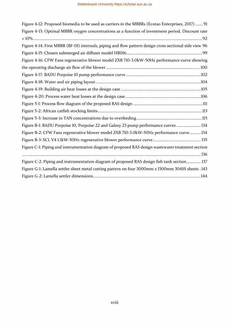
Figure 4-12: Proposed biomedia to be used as carriers in the MBBRs (Ecotao Enterprises, 2017) ....... 91

Figure 4-13: Optimal MBBR oxygen concentrations as a function of investment period. Discount rate

= 10% ........................................................................................................................................................ 92

Figure 4-14: First MBBR (BF-01) internals, piping and flow pattern design cross sectional side view 96

Figure 4-15: Chosen submerged air diffuser model HB016 .................................................................... 99

Figure 4-16: CFW Fans regenerative blower model ZXB 710-3.0kW-50Hz performance curve showing

the operating discharge air flow of the blower .................................................................................... 100

Figure 4-17: BADU Porpoise 10 pump performance curve ................................................................... 102

Figure 4-18: Water and air piping layout ............................................................................................... 104

Figure 4-19: Building air heat losses at the design case ........................................................................ 105

Figure 4-20: Process water heat losses at the design case .................................................................... 106

Figure 5-1: Process flow diagram of the proposed RAS design ............................................................... 111

Figure 5-2: African catfish stocking limits .............................................................................................. 113

Figure 5-3: Increase in TAN concentrations due to overfeeding ........................................................... 115

Figure B-1: BADU Porpoise 10, Porpoise 22 and Galaxy 23 pump performance curves ...................... 134

Figure B-2: CFW Fans regenerative blower model ZXB 710-3.0kW-50Hz performance curve .......... 134

Figure B-3: SCL V4 1.1kW-50Hz regenerative blower performance curve ........................................... 135

Figure C-1: Piping and instrumentation diagram of proposed RAS design wastewater treatment section

................................................................................................................................................................. 136

Figure C-2: Piping and instrumentation diagram of proposed RAS design fish tank section ............. 137

Figure G-1: Lamella settler sheet metal cutting pattern on four 3000mm x 1500mm 304SS sheets . 143

Figure G-2: Lamella settler dimensions ................................................................................................. 144


1

Chapter 1. Introduction to recirculating

aquaculture systems (RAS)

_________

1.1 Introduction

Fish production is achieved by two different means. Firstly, wild fish are caught in the sea, lakes and

rivers by fisheries. Secondly, fish are cultivated in farms (also known as aquaculture) employing a

variety of production systems, including ponds, floating cages, flow-through raceways and

recirculating aquaculture systems (RAS) (Timmons and Ebeling, 2007). Fish is an important food

source that has been growing steadily in terms of consumption per capita, with global annual

consumption increasing from 11.7 kg/capita in 1980 to 20.3 kg/capita in 2015 (FAOSTAT, 2017).

Aquaculture is reported as the world’s fastest growing agricultural industry with an average annual

growth in global production of 8% (based on statistics from 1980 to 2015) (World Bank, 2011). The

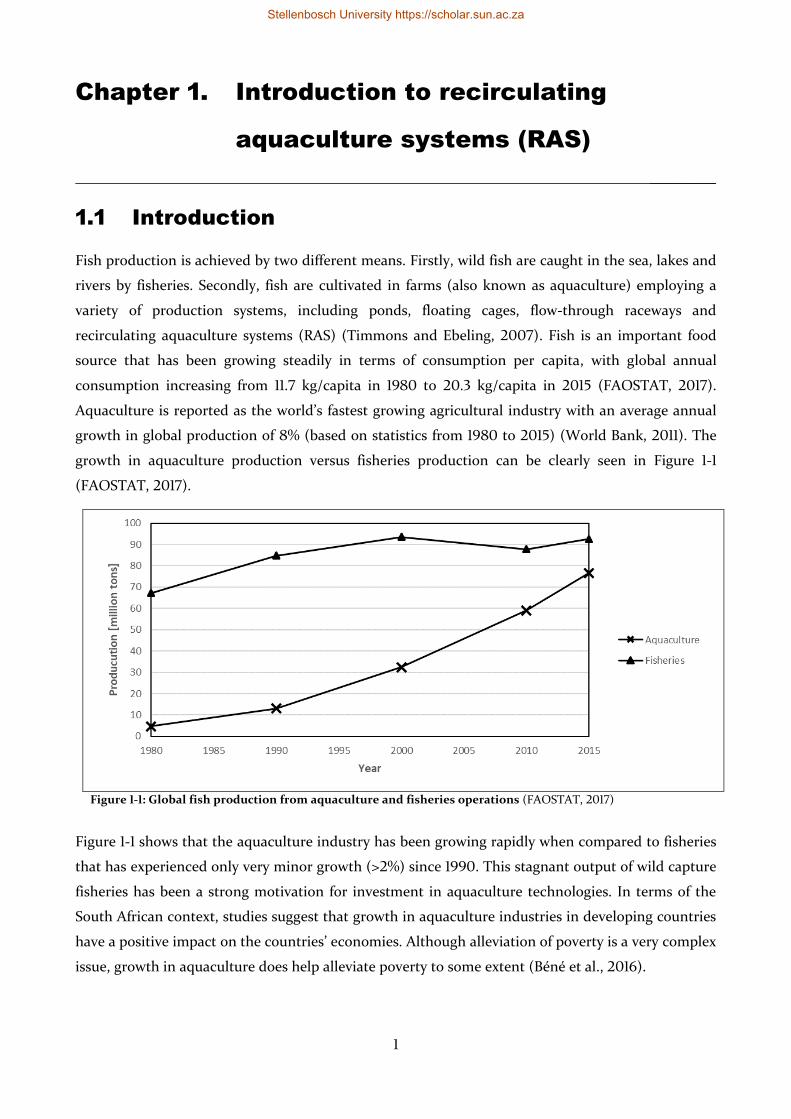
growth in aquaculture production versus fisheries production can be clearly seen in Figure 1-1

(FAOSTAT, 2017).

Figure 1-1: Global fish production from aquaculture and fisheries operations (FAOSTAT, 2017)

Figure 1-1 shows that the aquaculture industry has been growing rapidly when compared to fisheries

that has experienced only very minor growth (>2%) since 1990. This stagnant output of wild capture

fisheries has been a strong motivation for investment in aquaculture technologies. In terms of the

South African context, studies suggest that growth in aquaculture industries in developing countries

have a positive impact on the countries’ economies. Although alleviation of poverty is a very complex

issue, growth in aquaculture does help alleviate poverty to some extent (Béné et al., 2016).


2

1.2 Recirculating aquaculture systems (RASs)

Recirculating aquaculture systems (RAS) are, as the name implies, an aquaculture production system

where the water used for culturing the animals is treated and then recirculated within the system.

Effluent from the culturing tanks is treated using known wastewater treatment technologies, and

mostly consists of solids removal, biological nitrification of ammonia to nitrate, degassing of dissolved

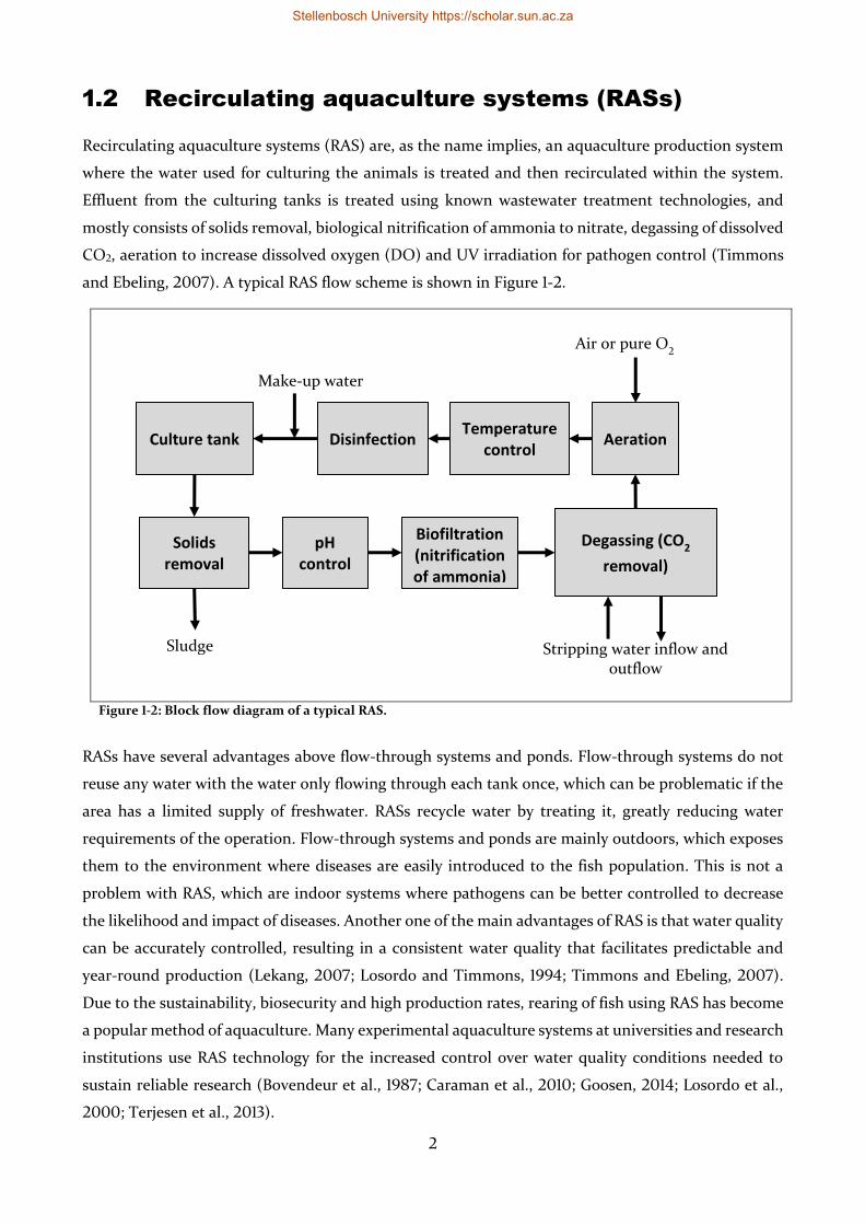
CO2, aeration to increase dissolved oxygen (DO) and UV irradiation for pathogen control (Timmons

and Ebeling, 2007). A typical RAS flow scheme is shown in Figure 1-2.

Figure 1-2: Block flow diagram of a typical RAS.

RASs have several advantages above flow-through systems and ponds. Flow-through systems do not

reuse any water with the water only flowing through each tank once, which can be problematic if the

area has a limited supply of freshwater. RASs recycle water by treating it, greatly reducing water

requirements of the operation. Flow-through systems and ponds are mainly outdoors, which exposes

them to the environment where diseases are easily introduced to the fish population. This is not a

problem with RAS, which are indoor systems where pathogens can be better controlled to decrease

the likelihood and impact of diseases. Another one of the main advantages of RAS is that water quality

can be accurately controlled, resulting in a consistent water quality that facilitates predictable and

year-round production (Lekang, 2007; Losordo and Timmons, 1994; Timmons and Ebeling, 2007).

Due to the sustainability, biosecurity and high production rates, rearing of fish using RAS has become

a popular method of aquaculture. Many experimental aquaculture systems at universities and research

institutions use RAS technology for the increased control over water quality conditions needed to

sustain reliable research (Bovendeur et al., 1987; Caraman et al., 2010; Goosen, 2014; Losordo et al.,

2000; Terjesen et al., 2013).

Culture tank

Solids removal

Degassing (CO2

removal)

Biofiltration (nitrification of ammonia)

Aeration Disinfection

Make-up water

Sludge Stripping water inflow and outflow

Air or pure O2

Temperature control

pH control


3

1.3 Motivation for the study

Stellenbosch University owns an experimental facility at Welgevallen (33° 56' 34.8'' S 18° 51' 57.6'' E).

This facility hosts various RAS for experimental work on Mozambique tilapia (Oreochromis

mossambicus) and African catfish (Clarias gariepinus). Under conditions of high stocking density and

multiple simultaneous trials, some of the experimental RAS have been unable to maintain optimal

water quality standards. In experimental work it is especially crucial to consistently maintain water

quality according to standards to gain conclusive results in terms of, for example, growth rates of

cultured animals. Due to the inability to maintain water quality during high biomass loading, periodic

water exchanges have been implemented to control water quality, which negates any advantages of

lower water usage that RAS should provide. In recent years, the Western Cape (including Stellenbosch)

has been subject to stringent water restrictions, thus having a well-functioning and high water-reuse

RAS able to maintain high water quality standards for experimental work is particularly important to

ensure high quality research which also utilizes water responsibly.

In the African context, better understanding of production of African catfish using RAS is crucial.

African catfish is already grown in Nigeria using RAS, but production thereof is limited due to lack of

knowledge of the technology and management of RAS (Akinwole and Faturoti, 2007). African catfish

is a fast-growing fish that is relatively easy to culture, making it an attractive option for food

production in developing countries. Interest has been shown in developing the market for African

catfish in South Africa as well (DAFF, 2018).

RAS technology in general is poorly understood in South Africa (DAFF, 2018), with only a few small

companies offering design work. Design of facilities producing high-end products such as Atlantic

salmon have been outsourced to international companies due to lack of knowledge on both the fish

species and the RAS technology (SalmonBusiness, 2018). Implementation of a commercial RAS

requires large capital investments and operating costs to run when compared to wild caught fish.

Therefore, high productivity in operations is required to make land-based fish production more

sustainable.

Thus, better understanding of RAS technology and the Welgevallen experimental systems would be

beneficial to research productivity and quality at Welgevallen and provide an opportunity for

experimentation of the RAS itself. These points motivated the research question that this study

attempted to answer: What methodology and parameters are appropriate for the design of an

experimental RAS? This study set out to answer the research question by establishing a design

methodology and demonstrating it practically by providing a design of a well-functioning RAS for use

at Welgevallen.


4

1.4 Objectives and scope of the study

This study aimed to establish a design methodology and provide a design of a new RAS capable of

culturing both African catfish and Mozambique tilapia.

Objective 1 - Determine through a literature survey the different technology options that can be used

in RAS and evaluate the maturity, benefits and disadvantages of these technologies.

Objective 2 - Develop or compile mathematical models to describe (1) biomass growth and waste

production, (2) the individual wastewater treatment unit operations, (3) fluid transport

and (4) energy requirements in the RAS.

Objective 3 - Apply the RAS models to (1) evaluate the current Welgevallen RAS to identify

equipment that can be reused or cost effectively altered and (2) design a new RAS based

on retrofitting within existing infrastructure.

Objective 4 - Compile an operating guide to aid in successful operation of the designed RAS.

The scope of the design was limited to conceptual engineering design due to time constraints. The

capital costs and operating costs of the proposed facility was to be determined. The design was to be

described using:

1) Top-view layout of the RAS

2) Process flow diagram (PFD) of the RAS showing the major equipment and pipelines.

3) Piping and instrumentation diagram (P&ID) of the RAS showing all piping, valves and

equipment in detail.

4) Data sheets of each major piece of equipment describing critical information.


5

1.5 Structure of the thesis

It should be noted that the work contained in this thesis was done using the engineering design

method rather than the scientific method. As with the scientific method, the engineering design

method focused on thoroughly defining the problem, identifying constraints and methods through a

review of available literature. Where the engineering design method is different is that the study

focused on formulating the final design package and product rather than observation and discovery of

phenomenon through experimentation. The various chapters of this thesis show the design steps taken

and presents the final design proposal at the end. Here follows a brief description of each chapter:

Chapter 1 Introduction to recirculating aquaculture systems (RAS)

The importance of RAS is motivated in this chapter along with the description of the project scope

and objectives.

Chapter 2 Literature survey of RAS technology

Important water quality parameters are described in this chapter along with the allowable limits and

measurement methods. Available RAS water treatment technologies are listed and discussed in this

chapter.

Chapter 3 Steady state RAS modeling methods

All the models used for the sizing of the equipment are described in this chapter. This consists of the

fish growth model, waste production estimates, biofilter reactor models, sedimentation model, sand

filter model, aeration model and heat transfer modeling of the facility. Motivation for the use of a

certain model is given where needed.

Chapter 4 Conceptual design results

The main design decisions are stated in this chapter. Motivation for the decisions are supported by

use of the models described in Chapter 3. The selection of technologies and sizing of equipment is

presented in this chapter. Sensitivity analyses are presented in this chapter that investigate the

sensitivity of equipment sizes to changes in certain design parameters.

Chapter 5 System design proposal

A breakdown of sizes and costs for the redesigned system is presented and discussed. Drawings of the

proposed facility is given. A management plan for successful operation of the proposed facility is given

as well as possible areas of future process optimization.


6

Chapter 2. Literature survey of RAS technology

_________

An overview of RAS technologies was essential to gain knowledge of the benefits and disadvantages of

the various options for each unit operation and achieve Objective 1 of the study (see section 1.4). This

allowed the choice of modeling methods to be more focused on specific technologies. Note that the

technology choices are motivated in Chapter 4 as part of the design process narrative. The literature

survey of RAS included water quality parameters, biofiltration, solids removal, aeration, degassing of

carbon dioxide, UV irradiation, water heating, air conditioning and waste management.

2.1 Water quality parameters

Good management of water quality parameters in RAS culture is crucial. Fish species can only survive

within a certain range of each water quality parameter with the ranges varying between different

species. The water quality parameters for both the African catfish and Mozambique tilapia was

investigated as the system was to be designed to be capable of culturing either species. Within the

allowable range of a water quality parameter exists an optimal value where optimal growth and health

of the fish is observed, which is required for optimal production performance and therefore economic

performance. Considerable research has been devoted to determining the allowable limits for different

species as well as the optimal parameter values. The aim of this section is to (1) define the critical

parameters, (2) discuss why each of the critical parameters are important in fish production, (3)

determine the allowable limits and optimal values reported in literature for African catfish and

Mozambique tilapia and (4) state how each critical parameter is measured.

2.1.1 Dissolved oxygen concentration

Dissolved oxygen (DO) in the water is utilized by fish during respiration and is thus crucial for the

survival of fish. A notable exception is the African catfish, which does have lungs capable of breathing

air when crucially needed. However, the air breathing ability of African catfish was not considered in

the design as it is only likely to occur at DO concentrations far below the optimal. Oxygen in fish drives

all biological processes including digestion and growth. DO concentrations in water is important due

to limited gill surface area that can take up oxygen, thus limiting the rate at which oxygen can be taken

up (Tran-Duy et al., 2008), and sub-optimal DO concentrations impair growth rates of fish. Buentello

et al. (2000) found that weight gain and feed intake both decreased with decreasing DO

concentrations in channel catfish (Ictalurus punctatus) culture.

Timmons and Ebeling (2007) report a minimum safe DO concentration of 2 – 3 mg/L, below which

fish can start suffocating. However, they recommend DO concentrations of 5 mg/L or higher to ensure

optimal growth of warm-water freshwater fish. A DO concentration of 5 mg/L or higher is also

recommended for commercial African catfish production (DAFF, 2018). Tilapia production is


7

recommended to have DO concentrations higher than 4 mg/L (Eding et al., 2006). For the purposes

of designing a dual-purpose RAS, a design value of 5 mg/L would be suitable as it is optimal for both

African catfish and tilapia.

DO levels have to be measured regularly due to the importance of oxygen for the survival of fish.

Continuous monitoring is sometimes necessary if stocking densities are high. Monitoring of DO levels

can be done analytically with the Winkler method or be measured using a DO probe, as is commonly

done in RAS. DO meters work by placing an electrode in the water, which produces a signal that is

proportional to the DO level in the water (Timmons and Ebeling, 2007).

2.1.2 Temperature

Fish are poikilothermic, which means that their body temperature is regulated by the surrounding

water temperature. Therefore, there is only a certain temperature range for each fish species in which

they can survive. There is also an optimum growing temperature for each fish. Fish are classified into

3 different groups:

• Cold-water = <15oC

• Cool-water = 15oC – 20oC

• Warm-water = >20oC

Both African catfish and tilapia are warm-water fish. Various recommendations for water temperatures

are found in literature. Recommendations for African catfish are 25oC – 27oC (Eding et al., 2006) and

24oC – 26oC (Akinwole and Faturoti, 2007), while those for tilapia are 24oC – 30oC (Eding et al., 2006)

and 28oC – 32oC (Timmons and Ebeling, 2007). When cultivated beyond these recommended ranges,

animals will grow sub-optimally and be susceptible to disease. For example, in a trial with African

catfish a high rate of mortalities was observed at water temperatures between 30oC and 35oC induced

by high environmental temperatures (Oluwaseyi, 2016). The mortalities were proposed to be due to a

condition called bloat that is a consequence of the high water temperatures (Oluwaseyi, 2016). This

would suggest that the water temperature of 30oC was too high for African catfish, and a RAS should

rather be controlled at the recommended temperatures of 24oC – 27oC when growing African catfish.

A suitable design temperature would be 27oC as it is within the recommended optimal ranges of both

African catfish and tilapia. This is an acceptable choice as there is an example of an experimental RAS

used to rear both African catfish and tilapia at 26.0oC ±0.7oC (Mota et al., 2015). African catfish has

also been reared in an experimental system at 27.0oC (Schram et al., 2010).

The main method of measuring temperature is by using temperature probes included in DO meters

and pH meters. Mercury thermometers are no longer used due to the risk involved with mercury leaks

into the fish culture tanks (Timmons and Ebeling, 2007).


8

2.1.3 Ammonia, nitrite and nitrate concentrations

Nitrogenous wastes are pollutants that enter the water through various means, and mainly originate

from the feed. Urea, uric acid and amino acids are excreted by fish through gill diffusion, gill cation

exchange, urine and feces. Nitrogenous wastes can also enter the water through uneaten feed,

decomposing biomass and nitrogen gas from the atmosphere. The most important nitrogenous waste

found in aquaculture wastewater is ammonia (Timmons and Ebeling, 2007). Ammonia is mostly

harmless in its ionized form, ammonium (NH4+), but is toxic to fish in its un-ionized form, ammonia

(NH3). Ammonium and ammonia are in equilibrium in water due to deprotonation of ammonia shown

in equation (2.1).

𝑁𝐻3 + 𝐻2𝑂 → 𝑁𝐻4+ + 𝑂𝐻− (2.1)

Thus, ammonia needs to be removed from the RAS water and is done through biofiltration, which

involves the oxidation of ammonium (NH4+) to nitrite (NO2

-) and nitrite to nitrate (NO3-) through the

metabolism of autotrophic bacteria (see section 2.2.1).

For ease of calculation, inorganic nitrogen compounds are often expressed by the amount of nitrogen

they contain, such as NH3-N (un-ionized ammonia nitrogen), NH4+-N (ionized ammonium nitrogen),

NO2—N (nitrite nitrogen), NO3

—N (nitrate nitrogen) and TAN (total-ammonia-nitrogen), which is the

sum of NH3-N and NH4+-N.

2.1.3.1 Ammonia

The ratio of NH3-N to NH4+-N is a function of pH, temperature and salinity. An equation for the

prediction of un-ionized ammonia fraction was developed by Emerson et al., (1975).

𝐶𝑁𝐻3−𝑁 =𝐶𝑇𝐴𝑁

10(𝑝𝐾𝑎−𝑝𝐻) + 1 (2.2)

where

𝐶𝑁𝐻3−𝑁 = Un-ionized ammonia concentration [𝑚𝑔 𝐿⁄ ]

𝐶𝑇𝐴𝑁 = Total-ammonia-nitrogen concentration [𝑚𝑔 𝐿⁄ ]

𝑝𝐾𝑎 = Acid dissociation constant

𝑝𝐾𝑎 can be estimated using equation (2.3):

𝑝𝐾𝑎 = 0.0901821 +2729.92

𝑇 (2.3)

where

𝑇 = Temperature [𝐾]

Thus equations (2.2) and (2.3) can be used to predict the concentration of NH3-N in freshwater when

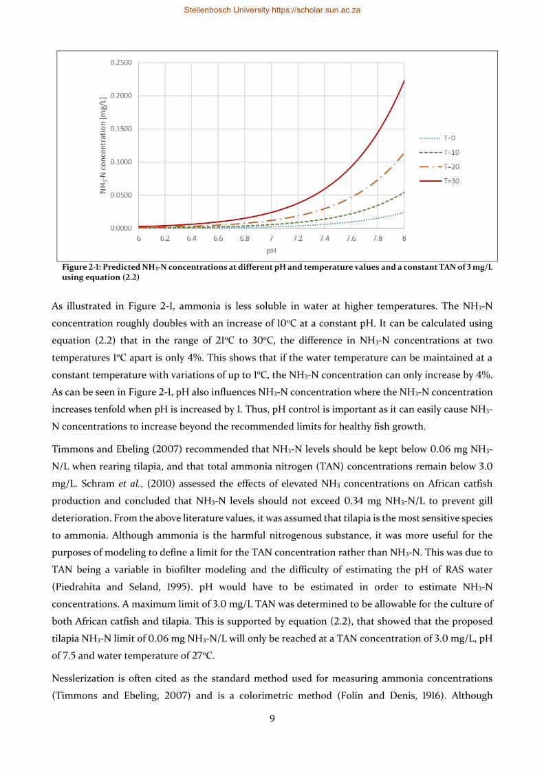
the pH and temperature is known. Figure 2-1 is a graphical depiction of equation (2.2), showing the

effect of both pH and temperature on NH3-N concentrations.


9

Figure 2-1: Predicted NH3-N concentrations at different pH and temperature values and a constant TAN of 3 mg/L using equation (2.2)

As illustrated in Figure 2-1, ammonia is less soluble in water at higher temperatures. The NH3-N

concentration roughly doubles with an increase of 10oC at a constant pH. It can be calculated using

equation (2.2) that in the range of 21oC to 30oC, the difference in NH3-N concentrations at two

temperatures 1oC apart is only 4%. This shows that if the water temperature can be maintained at a

constant temperature with variations of up to 1oC, the NH3-N concentration can only increase by 4%.

As can be seen in Figure 2-1, pH also influences NH3-N concentration where the NH3-N concentration

increases tenfold when pH is increased by 1. Thus, pH control is important as it can easily cause NH3-

N concentrations to increase beyond the recommended limits for healthy fish growth.

Timmons and Ebeling (2007) recommended that NH3-N levels should be kept below 0.06 mg NH3-

N/L when rearing tilapia, and that total ammonia nitrogen (TAN) concentrations remain below 3.0

mg/L. Schram et al., (2010) assessed the effects of elevated NH3 concentrations on African catfish

production and concluded that NH3-N levels should not exceed 0.34 mg NH3-N/L to prevent gill

deterioration. From the above literature values, it was assumed that tilapia is the most sensitive species

to ammonia. Although ammonia is the harmful nitrogenous substance, it was more useful for the

purposes of modeling to define a limit for the TAN concentration rather than NH3-N. This was due to

TAN being a variable in biofilter modeling and the difficulty of estimating the pH of RAS water

(Piedrahita and Seland, 1995). pH would have to be estimated in order to estimate NH3-N

concentrations. A maximum limit of 3.0 mg/L TAN was determined to be allowable for the culture of

both African catfish and tilapia. This is supported by equation (2.2), that showed that the proposed

tilapia NH3-N limit of 0.06 mg NH3-N/L will only be reached at a TAN concentration of 3.0 mg/L, pH

of 7.5 and water temperature of 27oC.

Nesslerization is often cited as the standard method used for measuring ammonia concentrations

(Timmons and Ebeling, 2007) and is a colorimetric method (Folin and Denis, 1916). Although


10

nesslerization is still used at existing facilities (Terjesen et al., 2013; Fernandes, Pedersen and Pedersen,

2017), this method has been replaced as a standard quantification method due to the use of mercury

in the analysis. Alternatives to nesslerization are an ammonia-selective electrode method and a

phenate spectrophotometric method that can measure concentrations from 0.03 to 1400 mg NH3-N/L

and 0.02 to 2.0 mg NH3-N/L respectively. The phenate method involves the formation of indophenol

from ammonia, hypochlorite and phenol and is quantified using a spectrophotometer (APHA, 1998).

Ammonia concentration measurements have also been done using ion chromatography, which is both

expensive and time consuming (Brazil, 2006).

2.1.3.2 Nitrite

Nitrite (NO2-) is the intermediate product of nitrification (see Section 2.2.1) and has been proven to

be toxic to fish (Hilmy et al., 1987). Freshwater fish must continually take up Cl- ions through their

gills to make up for ions lost through urine and passive efflux across the gills. The presence of nitrite

causes the nitrite ions to preferentially be taken up instead of Cl-. Nitrite ions enter the blood stream

and diffuse into red blood cells, where these ions in the red blood cells react with iron found in

hemoglobin, forming methemoglobin that reduces the overall oxygen carrying capacity of the blood.

High levels of methemoglobin can cause fish mortalities (Kroupova et al., 2005). Fish have been shown

to acclimatize to nitrite over time, increasing their resistance to toxic effects (Kroupova et al., 2005).

However, a sudden increase in nitrite concentrations could be lethal.

Nitrite toxicity is affected by a range of factors namely: length of exposure, chloride concentration,

bromide concentration, calcium concentration, sodium concentration, ammonia concentration, pH,

dissolved oxygen, temperature, fish species and fish size (Kroupova et al., 2005). The most significant

factor influencing nitrite toxicity is the chloride concentration. Nitrite toxicity has been found to

greatly decrease when chloride ions are present in the water (Tomasso et al., 1979). Thus a certain

ratio of chloride to nitrite must be maintained to prevent the toxic effects of nitrite on fish. Timmons

and Ebeling (2007) recommended a 20 to 1 mass ratio of Cl- to NO2- and that the NO2-N concentration

should be kept below 1.0 mg NO2-N/L when rearing tilapia. Losordo et al. (2000) have successfully

operated an intensive tilapia RAS by maintaining 100 mg Cl-/L at an average NO2-N concentration of

1.83 mg NO2-N/L. These higher nitrite levels were reported to be typical of a biofilter that is still

developing a stable biofilm. Thus, the steady state design nitrite concentration should be below 1.0 mg

NO2-N/L.

A colorimetric method is the most common method of measuring nitrite concentration in water and

requires the use of a spectrophotometer or filter photometer (APHA, 1998). Ion chromatography was

used for nitrite concentration measurements by Brazil (2006), which is both expensive and time

consuming compared to other methods. As an alternative to the colorimetric method, a cadmium

reduction method was used for nitrite concentration measurements by Losordo et al. (2000).


11

2.1.3.3 Nitrate

Nitrate (NO3-) is the final product of the nitrification process (see Section 2.2.1). Nitrate is only

removed from a RAS through water exchange or denitrification (reduction of nitrate to nitrogen gas).

If the RAS has a high water reuse ratio, nitrate can accumulate in the system (Timmons and Ebeling,

2007). Identically to nitrite, nitrate is suggested to be toxic due to uptake in the blood and the

subsequent conversion of hemoglobin to methemoglobin. The uptake of nitrate is less profound than

nitrite and is thus less toxic (Camargo et al., 2005).

Timmons and Ebeling (2007) recommended nitrate concentrations be maintained below 400 mg

NO3-N/L. Losordo et al. (2000) operated a tilapia farm at nitrate concentrations of 200 – 250 mg NO3-

N/L. Schram et al. (2014) assessed the effects of nitrate on the physiology, growth and feed intake of

African catfish and recommended that nitrate concentrations should not exceed 140 mg NO3-N/L. The

design maximum nitrate concentration was thus chosen to be 140 mg NO3-N/L.

Various methods can be used for nitrite measurements, namely (1) ultraviolet method, (2) ion

chromatography, (3) capillary ion electrophoresis, (4) nitrate electrode method, (5) cadmium

reduction method and (6) automated cadmium reduction methods (APHA, 1998). Ion

chromatography was used for nitrate concentration measurements by Brazil (2006).

2.1.4 pH, alkalinity and hardness

pH is a measure of how acidic or basic a solution is and is defined in equation (2.4) (Stumm and

Morgan, 1995):

𝑝𝐻 = −log {𝐻+} (2.4)

where

{𝐻+} = Activity of hydrogen ions (activity is the measure of the effective concentration of a species in a mixture)

pH is important in RAS for a variety of reasons. Both the fish and bacteria have a range of pH values

that they can survive and thrive in. However, the most crucial effect of pH is its effect on the ratio of

NH4+ to NH3 (see section 2.1.3.1) At the maximum values of 0.06 mg NH3-N/L and 3.0 mg TAN/L, the

maximum allowable pH would be 7.5, calculated using equation (2.2). Timmons and Ebeling (2007)

recommended an optimal pH range of 6.5 to 9.0 for freshwater fish. Tilapia has been successfully

reared in a system with a pH varying between 6.9 and 7.4. (Losordo et al., 2000) Thus, a steady state

design pH of 7.0±0.2 would be acceptable. pH is measured using pH meters calibrated using standard

solutions (APHA, 1998).

Alkalinity is the acid neutralizing capacity of water and is defined as the amount of titratable bases

present in the water. Alkalinity is expressed as the equivalent of milligrams calcium carbonate (CaCO3)

per liter (APHA, 1998). CO3- and HCO3

- are the main ions contributing to alkalinity. Since HCO3- is

consumed in nitrification reactions (see section 2.2.1), alkalinity often needs to be increased by adding


12

a supplement such as sodium bicarbonate (NaHCO3) (Timmons and Ebeling, 2007; Bovendeur et al.,

1987). Alkalinity, pH and carbon dioxide concentrations are linked and thus the required alkalinity

depends on pH and carbon dioxide concentrations. Total alkalinity is measured using a titration

technique by changing the pH to 8.3 first using a phenolphthalein indicator and then to 4.5 using a

bromocresol green or a mixed bromocresol green-methyl red indicator (APHA, 1998).

Hardness is defined as the sum of the bivalent metal ions and is expressed as the equivalent of mg

CaCO3/L (APHA, 1998). Calcium and magnesium are important minerals for fish bone and scale

growth (Wurts, 2002). Wurts (2002) recommended that calcium hardness in aquaculture water

should range between 75 and 200 mg CaCO3/L. Timmons and Ebeling (2007) recommended that total

water hardness should be kept above the equivalent of 100 mg CaCO3/L in a commercial fish tank. An

EDTA titrimetric method is used to measure total water hardness (APHA, 1998).

2.1.5 Carbon dioxide concentration

Dissolved carbon dioxide in water can be inhibitory to fish health at high levels. The carbon dioxide

concentration in the fish’s blood can increase, decreasing the amount of oxygen that the hemoglobin

in the blood can transport. This can lead to respiratory distress in fish (Timmons and Ebeling, 2007).

An upper limit of 15-20 mg CO2/L is recommended when rearing tilapia (Timmons and Ebeling, 2007)

and 25 mg CO2/L when rearing African catfish. (Eding et al., 2006). However, it was stated by these

sources that carbon dioxide limits are difficult to define and should be used as rough guidelines. The

chosen maximum allowable carbon dioxide concentration was 15 mg/L to remain conservative and

allow for the system to be suitable for both African catfish and tilapia. Dissolved carbon dioxide is

inferred using a nomograph which requires knowledge of the pH and total alkalinity (Timmons and

Ebeling, 2007).

2.1.6 Solids concentration

Solids in water are classified into two main categories, namely total suspended solids (TSS) and total

dissolved solids (TDS). TSS is defined as the solids larger than 2.0 µm and TDS as the solids smaller

than 2.0 µm (APHA, 1998). TDS is also known as salinity (see section 2.1.7).

Feces and uneaten feed are the main sources of TSS in water. The presence of these particles increase

biochemical oxygen demand in the water (BOD) and releases toxins such as ammonia into the water

(Baccarin and Camargo, 2005). Suspended solids negatively affect biofiltration by attaching to the

biofilm, increasing BOD and thereby decreasing nitrification rates (Eding et al., 2006). In other words,

the presence of suspended solids decreases the efficiency of biofilters. Chapman et al. (1987) have

shown suspended solids within the size range of 5 – 10 µm to be toxic to rainbow trout. No research

on the effects of varying suspended solid particle sizes on either tilapia or African catfish was found.

Suspended solids can negatively affect fish health by damaging gills and carrying pathogens. Current

research suggests that generally the TSS concentration is not a critical parameter for fish health when

compared to dissolved oxygen, carbon dioxide, temperature or ammonia (Timmons and Ebeling,


13

2007). However, the fact that suspended solids increases BOD, total ammonia nitrogen

concentrations and decreases biofilter efficiency warrants the rapid removal of TSS within a RAS.

Timmons and Ebeling (2007) recommended an upper limit for TSS concentration at 25 mg/L and 10

mg/L for long-term operation of freshwater fish culture. 25 mg/L is recommended as the upper limit

for African catfish (Eding et al., 2006). A limit of 15 mg/L has also been recommended (Chen et al.,

1994). Tilapia have been reported to show no adverse effects in well-being when the TSS concentration

was 80 mg/L with all other water quality parameters being acceptable (Timmons and Ebeling, 2007).

For TSS concentration data collection, TSS concentration is measured using standard method number

2540D, which is sampling, filtration of the sample through a glass-fiber filter, constant drying of the

sample at 103 to 105oC and measurement of the filter mass increase (APHA, 1998).

2.1.7 Salinity

Salinity is the concentration of dissolved salts in the water (APHA, 1998) and is expressed as parts per

million (ppm) or milligrams of salt per liter of water. Freshwater aquaculture systems are generally

maintained at a salinity of 2000 to 3000 ppm. The TDS is equal to the salinity and commonly includes

calcium, sodium, potassium, bicarbonate, chloride and sulfate (Timmons and Ebeling, 2007).

The most efficient methods of measuring salinity are indirectly using electrical conductivity, water

density, speed of sound in the water, or refractive index. Electrical conductivity is the most precise and

convenient of these methods and is thus the most used method for determining salinity (APHA, 1998).

2.1.8 Biochemical oxygen demand (BOD)

Biochemical oxygen demand (BOD) is defined as the oxygen that can be consumed through oxidation

of organic matter by microorganisms. BOD can be expressed as either ultimate BOD (BODU) or 5-day

BOD (BOD5). BODU is a measure of the oxygen consumed when all carbonaceous and nitrogenous

organic matter have been biologically oxidized. BOD5 is a measure of the oxygen consumed by

biological oxidation of organic matter after a 5-day incubation period at 20oC. Most of the

carbonaceous organic matter is oxidized within the first 5 days of incubation, with minimal oxidation

of nitrogenous organic matter by nitrifying bacteria (APHA, 1998). Thus, it can be assumed that BOD5

is equal to the carbonaceous biochemical oxygen demand (CBOD5), which is a measure of the oxygen

consumed by heterotrophic biological oxidation of carbonaceous organic matter. BOD differs from

chemical oxygen demand (COD), which is the oxygen consumed through oxidation of organic matter

using a chemical oxidant. This means that COD accounts for both the biodegradable and non-

biodegradable portions of the organic matter (APHA, 1998).

High levels of BOD5 in RAS effluent can be harmful to the environment and requires further biological

treatment before discharge can be permitted. High levels of BOD5 in the recirculating water results in

increased heterotrophic bacterial populations, inhibiting nitrifying bacteria in the biofilter through

decreased availability of dissolved oxygen (Eding et al., 2006; Rusten et al., 2006). Specific limits for


14

BOD5 in RAS were difficult to define as, by itself, it does not have any negative effects on fish

production. The negative effect of BOD5 occurs via impacts on the biofilter performance and has been

accounted for in the biofilter modeling (see section 3.4.6.2).

2.1.9 Total dissolved gas pressure (TGP)

Supersaturation of gas in aquaculture water can cause gas bubble disease, usually leading to high

mortality rates in fish populations (Weitkamp and Katz, 1980). Gas supersaturation can occur in a RAS

when using submerged air diffusers due to hydrostatic pressure increasing the saturation

concentrations of dissolved gasses at the diffuser location. The degree of gas supersaturation is

determined by calculating the total dissolved gas pressure (TGP) by gas tensions (see section 3.6.2).

The water is considered supersaturated with gas if the TGP exceeds the local barometric pressure (BP).

Allowable limits of TGP in fish tanks are defined by (1) the %TGP, which is the ratio between TGP and

atmospheric pressure and (2) differential pressure (DP), which is TGP minus BP. For example, if TGP

and BP equals 836 mmHg and 760 mmHg respectively, the %TGP will be 110%. A study observed no

gas bubble disease at %TGP of 106% (Weitkamp and Katz, 1980). It is recommended that the DP in

intensive warm-water RAS not exceed 20 mmHg (Watten, 1994).


15

2.2 Biofiltration

Biofiltration is the process of removing ammonia from wastewater through biological nitrification

reactions. Nitrification is done by nitrifying bacteria that form part of a biofilm on solid media placed

in biofilter units. Biofiltration is considered a crucial process step in RAS that requires careful design

considerations (Timmons and Ebeling, 2007) and was thus a major focus of this thesis. Modeling of

biofilters is discussed in section 3.4.

2.2.1 Nitrification

Nitrification is the oxidation of ammonia to nitrite, followed by the oxidation of nitrite to nitrate. The

oxidation of ammonia to nitrite and nitrite to nitrate is done by the autotrophic bacteria Nitrosomonas

and Nitrobacter respectively. These nitrification reactions are given by equations (2.5) and (2.6)

(Henze et al., 1997).

Nitrosomonas: 𝑁𝐻4+ +

3

2 𝑂2 → 𝑁𝑂2

− + 𝐻2𝑂 + 2 𝐻+ (2.5)

Nitrobacter: 𝑁𝑂2− +

1

2 𝑂2 → 𝑁𝑂3

− (2.6)

Autotrophic bacteria use CO2 as their carbon source. The reactions for cell growth is given in equations

(2.7) and (2.8) with the compound C5H7NO2 representing the bacterial biomass (Henze et al., 1997).

15 𝐶𝑂2 + 13 𝑁𝐻4+ → 10 𝑁𝑂2

− + 3 𝐶5𝐻7𝑁𝑂2 + 4 𝐻2𝑂 + 23 𝐻+ (2.7)

5 𝐶𝑂2 + 𝑁𝐻4+ + 10 𝑁𝑂2

− + 2 𝐻2𝑂 → 10 𝑁𝑂3− + 𝐶5𝐻7𝑁𝑂2 + 𝐻+ (2.8)

In addition to using the carbonate equilibrium system (see APPENDIX E), equations (2.5) and (2.7)

are combined to yield equation (2.9). Equations (2.6) and (2.8) are also combined to yield equation

(2.10).

80.7 𝑁𝐻4+ + 114.55 𝑂2 + 160.4 𝐻𝐶𝑂3

− → 𝐶5𝐻7𝑁𝑂2 + 79.7 𝑁𝑂2− + 82.7 𝐻2𝑂 + 155.4 𝐻2𝐶𝑂3 (2.9)

134.5 𝑁𝑂2− + 𝑁𝐻4

+ + 62.25 𝑂2 + 𝐻𝐶𝑂3− + 4 𝐻2𝐶𝑂3 → 𝐶5𝐻7𝑁𝑂2 + 134.5 𝑁𝑂3

− + 3 𝐻2𝑂 (2.10)

Within a biofilter, the substrates for the metabolism reactions diffuse into the biofilm from the bulk

water and subsequently the products of the reactions (metabolites) diffuse back into the bulk water.

The two main substrates in equation (2.9) are ammonium (measured as TAN) and oxygen. Thus a

biofilter can be either TAN diffusion limited or oxygen diffusion limited (Eding et al., 2006).

2.2.2 Types of biofilters

Different types of biofilters are commonly used in wastewater treatment and RASs. As previously

mentioned, nitrifying bacteria are grown on solid media to form a biofilm, which is known as the fixed

film type of biofilter. Biofilters operating without solid media are classified as suspended growth

biofilters where heterotrophic bacteria are grown in suspension (Timmons and Ebeling, 2007)

Suspended growth biofilters are considered to be less stable than fixed film biofilters (Malone and


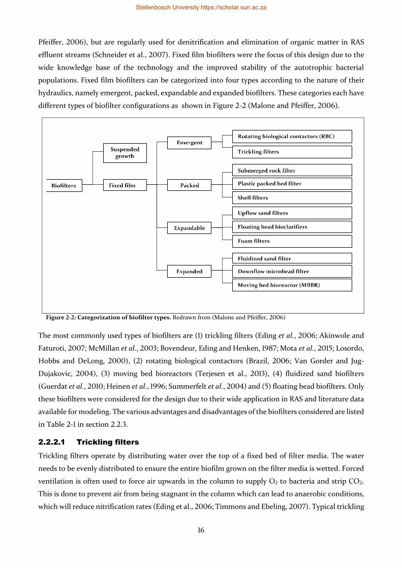
16

Pfeiffer, 2006), but are regularly used for denitrification and elimination of organic matter in RAS

effluent streams (Schneider et al., 2007). Fixed film biofilters were the focus of this design due to the

wide knowledge base of the technology and the improved stability of the autotrophic bacterial

populations. Fixed film biofilters can be categorized into four types according to the nature of their

hydraulics, namely emergent, packed, expandable and expanded biofilters. These categories each have

different types of biofilter configurations as shown in Figure 2-2 (Malone and Pfeiffer, 2006).

Figure 2-2: Categorization of biofilter types. Redrawn from (Malone and Pfeiffer, 2006)

The most commonly used types of biofilters are (1) trickling filters (Eding et al., 2006; Akinwole and

Faturoti, 2007; McMillan et al., 2003; Bovendeur, Eding and Henken, 1987; Mota et al., 2015; Losordo,

Hobbs and DeLong, 2000), (2) rotating biological contactors (Brazil, 2006; Van Gorder and Jug-

Dujakovic, 2004), (3) moving bed bioreactors (Terjesen et al., 2013), (4) fluidized sand biofilters

(Guerdat et al., 2010; Heinen et al., 1996; Summerfelt et al., 2004) and (5) floating bead biofilters. Only

these biofilters were considered for the design due to their wide application in RAS and literature data

available for modeling. The various advantages and disadvantages of the biofilters considered are listed

in Table 2-1 in section 2.2.3.

2.2.2.1 Trickling filters

Trickling filters operate by distributing water over the top of a fixed bed of filter media. The water

needs to be evenly distributed to ensure the entire biofilm grown on the filter media is wetted. Forced

ventilation is often used to force air upwards in the column to supply O2 to bacteria and strip CO2.

This is done to prevent air from being stagnant in the column which can lead to anaerobic conditions,

which will reduce nitrification rates (Eding et al., 2006; Timmons and Ebeling, 2007). Typical trickling


17

filters used in RAS vary from 0.15 – 5.0 m high (Wheaton et al., 1994a). Practical aspects of trickling

filter design and operations are described by Eding et al. (2006).

2.2.2.2 Rotating biological contactors (RBC)

A rotating biological contactor (RBC) is type of biofilter that consists of a rotating horizontal shaft

attached to the centers of multiple disks, acting as the media where the biofilm grows. The shaft is

located at the top of the water level with half of each disk being submerged. The disks are sufficiently

spaced to be close enough to provide high specific surface area and far enough apart to prevent

clogging (Wheaton et al., 1994a). The main aspect that sets RBC’s apart from other biofilters is that it

has mechanical moving parts, increasing the failure rate due to mechanical failure (Timmons and

Ebeling, 2007). Hochheimer and Wheaton (2000) discussed all the practical aspects of RBC design

and operation.

2.2.2.3 Fluidized sand biofilters (FSB)

Fluidized sand biofilters (FSB) are containers filled with a media of high specific surface area (usually

a type of sand) and operated by pumping water through the filter of a sufficient velocity to fluidize the

media. A mesh on the inlet pipe is installed to prevent backflow of media. The main costs associated

with FSBs are pumping costs due to the head loss through the media and the fact that water must be

pumped upwards through the filter (Wheaton et al., 1994a). FSBs are associated with systems required

to maintain excellent water quality of 0.1 – 0.5 mg TAN/L and < 0.1 – 0.3 mg NO2-N/L at the filter

discharge (Summerfelt, 2006). The practical aspects of design and management of FSB’s were

described by Summerfelt (2006).

2.2.2.4 Floating bead biofilters (FBB)

Floating bead biofilters (FBB) are similar in construction to FSBs but contain 3 – 5 mm polyethylene

beads as media with a specific gravity of roughly 0.91 and specific surface areas of 1150 – 1475 m2/m3.

The low specific gravity causes the beads to float. FBBs are operated in an up-flow configuration. FBBs

are also known as bioclarifiers due to the beads also acting as a granular filter (see section 2.3.2.2),

requiring periodic backwashing (Timmons and Ebeling, 2007).

2.2.2.5 Microbead filter

A microbead filter is similar in construction to FSBs and FBBs, but differs in the biomedia used, which

are polystyrene beads of a much lower density (16 kg/m3 bulk density) and are 1 – 3 mm in diameter.

Microbead filters are operated in a downflow configuration where water is distributed over the beads

and allowed to trickle downwards (Timmons and Ebeling, 2007).

2.2.2.6 Moving bed bioreactors (MBBR)

A moving bed bioreactor (MBBR) consists of floating biomedia with a specific gravity of 0.95. These

carriers are unlike floating bead filter and microbead filter media, as they are cylindrical structures

with inner and outer fins to increase specific surface area. The biomedia is constantly agitated by

aeration to achieve mixing of the water, supply oxygen and prevent clogging of the biofilm by abrasion


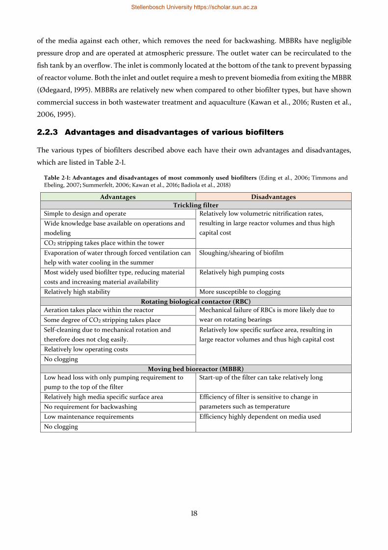
18

of the media against each other, which removes the need for backwashing. MBBRs have negligible

pressure drop and are operated at atmospheric pressure. The outlet water can be recirculated to the

fish tank by an overflow. The inlet is commonly located at the bottom of the tank to prevent bypassing

of reactor volume. Both the inlet and outlet require a mesh to prevent biomedia from exiting the MBBR

(Ødegaard, 1995). MBBRs are relatively new when compared to other biofilter types, but have shown

commercial success in both wastewater treatment and aquaculture (Kawan et al., 2016; Rusten et al.,

2006, 1995).

2.2.3 Advantages and disadvantages of various biofilters

The various types of biofilters described above each have their own advantages and disadvantages,

which are listed in Table 2-1.

Table 2-1: Advantages and disadvantages of most commonly used biofilters (Eding et al., 2006; Timmons and Ebeling, 2007; Summerfelt, 2006; Kawan et al., 2016; Badiola et al., 2018)

Advantages Disadvantages

Trickling filter

Simple to design and operate Relatively low volumetric nitrification rates,

resulting in large reactor volumes and thus high

capital cost

Wide knowledge base available on operations and

modeling

CO2 stripping takes place within the tower

Evaporation of water through forced ventilation can

help with water cooling in the summer

Sloughing/shearing of biofilm

Most widely used biofilter type, reducing material

costs and increasing material availability

Relatively high pumping costs

Relatively high stability More susceptible to clogging

Rotating biological contactor (RBC)

Aeration takes place within the reactor Mechanical failure of RBCs is more likely due to

wear on rotating bearings Some degree of CO2 stripping takes place

Self-cleaning due to mechanical rotation and

therefore does not clog easily.

Relatively low specific surface area, resulting in

large reactor volumes and thus high capital cost

Relatively low operating costs

No clogging

Moving bed bioreactor (MBBR)

Low head loss with only pumping requirement to

pump to the top of the filter

Start-up of the filter can take relatively long

Relatively high media specific surface area Efficiency of filter is sensitive to change in

parameters such as temperature No requirement for backwashing

Low maintenance requirements Efficiency highly dependent on media used

No clogging


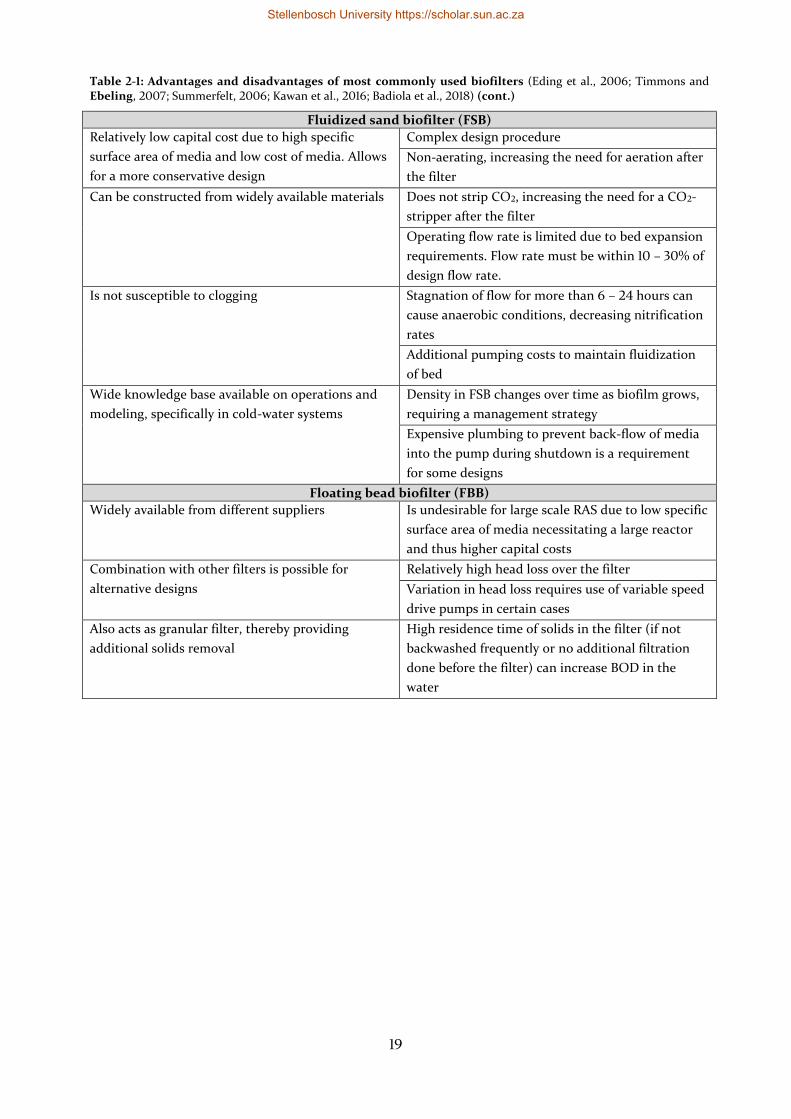
19

Table 2-1: Advantages and disadvantages of most commonly used biofilters (Eding et al., 2006; Timmons and Ebeling, 2007; Summerfelt, 2006; Kawan et al., 2016; Badiola et al., 2018) (cont.)

Fluidized sand biofilter (FSB)

Relatively low capital cost due to high specific

surface area of media and low cost of media. Allows

for a more conservative design

Complex design procedure

Non-aerating, increasing the need for aeration after

the filter

Can be constructed from widely available materials Does not strip CO2, increasing the need for a CO2-

stripper after the filter

Operating flow rate is limited due to bed expansion

requirements. Flow rate must be within 10 – 30% of

design flow rate.

Is not susceptible to clogging Stagnation of flow for more than 6 – 24 hours can

cause anaerobic conditions, decreasing nitrification

rates

Additional pumping costs to maintain fluidization

of bed

Wide knowledge base available on operations and

modeling, specifically in cold-water systems

Density in FSB changes over time as biofilm grows,

requiring a management strategy

Expensive plumbing to prevent back-flow of media

into the pump during shutdown is a requirement

for some designs

Floating bead biofilter (FBB)

Widely available from different suppliers Is undesirable for large scale RAS due to low specific

surface area of media necessitating a large reactor

and thus higher capital costs

Combination with other filters is possible for

alternative designs

Relatively high head loss over the filter

Variation in head loss requires use of variable speed

drive pumps in certain cases

Also acts as granular filter, thereby providing

additional solids removal

High residence time of solids in the filter (if not

backwashed frequently or no additional filtration

done before the filter) can increase BOD in the

water


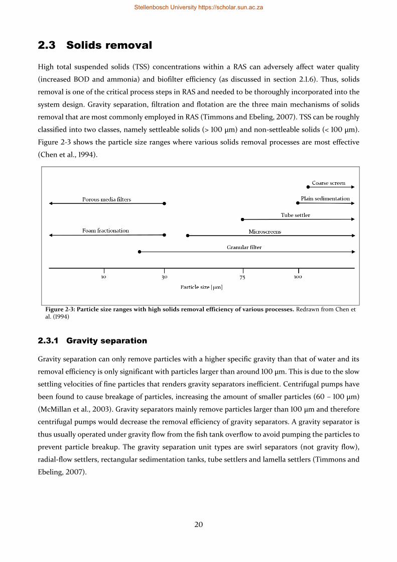
20

2.3 Solids removal

High total suspended solids (TSS) concentrations within a RAS can adversely affect water quality

(increased BOD and ammonia) and biofilter efficiency (as discussed in section 2.1.6). Thus, solids

removal is one of the critical process steps in RAS and needed to be thoroughly incorporated into the

system design. Gravity separation, filtration and flotation are the three main mechanisms of solids

removal that are most commonly employed in RAS (Timmons and Ebeling, 2007). TSS can be roughly

classified into two classes, namely settleable solids (> 100 µm) and non-settleable solids (< 100 µm).

Figure 2-3 shows the particle size ranges where various solids removal processes are most effective

(Chen et al., 1994).

Figure 2-3: Particle size ranges with high solids removal efficiency of various processes. Redrawn from Chen et al. (1994)

2.3.1 Gravity separation

Gravity separation can only remove particles with a higher specific gravity than that of water and its

removal efficiency is only significant with particles larger than around 100 µm. This is due to the slow

settling velocities of fine particles that renders gravity separators inefficient. Centrifugal pumps have

been found to cause breakage of particles, increasing the amount of smaller particles (60 – 100 µm)

(McMillan et al., 2003). Gravity separators mainly remove particles larger than 100 µm and therefore

centrifugal pumps would decrease the removal efficiency of gravity separators. A gravity separator is

thus usually operated under gravity flow from the fish tank overflow to avoid pumping the particles to

prevent particle breakup. The gravity separation unit types are swirl separators (not gravity flow),

radial-flow settlers, rectangular sedimentation tanks, tube settlers and lamella settlers (Timmons and

Ebeling, 2007).


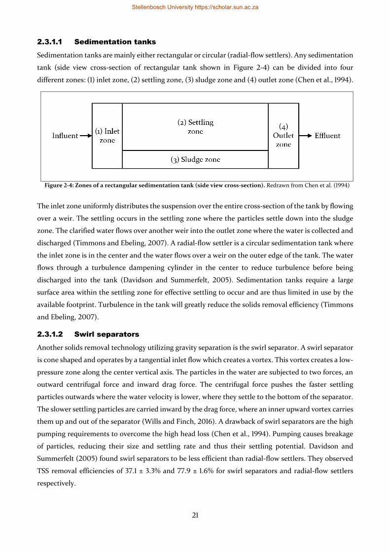
21

2.3.1.1 Sedimentation tanks

Sedimentation tanks are mainly either rectangular or circular (radial-flow settlers). Any sedimentation

tank (side view cross-section of rectangular tank shown in Figure 2-4) can be divided into four

different zones: (1) inlet zone, (2) settling zone, (3) sludge zone and (4) outlet zone (Chen et al., 1994).

Figure 2-4: Zones of a rectangular sedimentation tank (side view cross-section). Redrawn from Chen et al. (1994)

The inlet zone uniformly distributes the suspension over the entire cross-section of the tank by flowing

over a weir. The settling occurs in the settling zone where the particles settle down into the sludge

zone. The clarified water flows over another weir into the outlet zone where the water is collected and

discharged (Timmons and Ebeling, 2007). A radial-flow settler is a circular sedimentation tank where

the inlet zone is in the center and the water flows over a weir on the outer edge of the tank. The water

flows through a turbulence dampening cylinder in the center to reduce turbulence before being

discharged into the tank (Davidson and Summerfelt, 2005). Sedimentation tanks require a large

surface area within the settling zone for effective settling to occur and are thus limited in use by the

available footprint. Turbulence in the tank will greatly reduce the solids removal efficiency (Timmons

and Ebeling, 2007).

2.3.1.2 Swirl separators

Another solids removal technology utilizing gravity separation is the swirl separator. A swirl separator

is cone shaped and operates by a tangential inlet flow which creates a vortex. This vortex creates a low-

pressure zone along the center vertical axis. The particles in the water are subjected to two forces, an

outward centrifugal force and inward drag force. The centrifugal force pushes the faster settling

particles outwards where the water velocity is lower, where they settle to the bottom of the separator.

The slower settling particles are carried inward by the drag force, where an inner upward vortex carries

them up and out of the separator (Wills and Finch, 2016). A drawback of swirl separators are the high

pumping requirements to overcome the high head loss (Chen et al., 1994). Pumping causes breakage

of particles, reducing their size and settling rate and thus their settling potential. Davidson and

Summerfelt (2005) found swirl separators to be less efficient than radial-flow settlers. They observed

TSS removal efficiencies of 37.1 ± 3.3% and 77.9 ± 1.6% for swirl separators and radial-flow settlers

respectively.


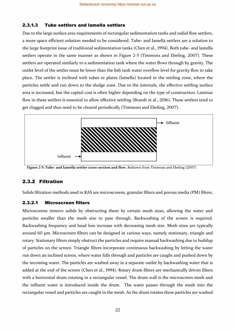
22

2.3.1.3 Tube settlers and lamella settlers

Due to the large surface area requirements of rectangular sedimentation tanks and radial flow settlers,

a more space efficient solution needed to be considered. Tube- and lamella settlers are a solution to

the large footprint issue of traditional sedimentation tanks (Chen et al., 1994). Both tube- and lamella

settlers operate in the same manner as shown in Figure 2-5 (Timmons and Ebeling, 2007). These

settlers are operated similarly to a sedimentation tank where the water flows through by gravity. The

outlet level of the settler must be lower than the fish tank water overflow level for gravity flow to take

place. The settler is inclined with tubes or plates (lamella) located in the settling zone, where the

particles settle and run down to the sludge zone. Due to the internals, the effective settling surface

area is increased, but the capital cost is often higher depending on the type of construction. Laminar

flow in these settlers is essential to allow effective settling (Brandt et al., 2016). These settlers tend to

get clogged and thus need to be cleared periodically (Timmons and Ebeling, 2007).

Figure 2-5: Tube- and lamella settler cross-section and flow. Redrawn from Timmons and Ebeling (2007)

2.3.2 Filtration

Solids filtration methods used in RAS are microscreens, granular filters and porous media (PM) filters.

2.3.2.1 Microscreen filters

Microscreens remove solids by obstructing them by certain mesh sizes, allowing the water and

particles smaller than the mesh size to pass through. Backwashing of the screen is required.

Backwashing frequency and head loss increase with decreasing mesh size. Mesh sizes are typically

around 60 µm. Microscreen filters can be designed in various ways, namely stationary, triangle and

rotary. Stationary filters simply obstruct the particles and require manual backwashing due to buildup

of particles on the screen. Triangle filters incorporate continuous backwashing by letting the water

run down an inclined screen, where water falls through and particles are caught and pushed down by

the incoming water. The particles are washed away in a separate outlet by backwashing water that is

added at the end of the screen (Chen et al., 1994). Rotary drum filters are mechanically driven filters

with a horizontal drum rotating in a rectangular vessel. The drum wall is the microscreen mesh and

the influent water is introduced inside the drum. The water passes through the mesh into the

rectangular vessel and particles are caught in the mesh. As the drum rotates these particles are washed


23

off by high pressure water jets from the outside, being caught in a separate outlet stream. Other

examples of microscreen filters are disc filters and inclined belt filters (Timmons and Ebeling, 2007).

Fernandes et al. (2015) investigated the effects of different drum filter mesh sizes on particle count,

nitrification kinetics and fish health. Although particle counts decreased, mesh sizes between 20 – 100

µm had no measurable impact on nitrification kinetics or fish health.

2.3.2.2 Granular filters

Granular filters capture particles by deposition onto media within the filter and can capture a wide

range of particle sizes (> 20 µm). Three types of granular filters are typically used, namely downflow

sand filters, upflow sand filters and bead filters (Chen et al., 1994). Due to the high head loss through

granular filters, a pump is required to pressurize the water to enable flow through the filter (Lekang,

2007).

2.3.2.3 Porous media filters

Porous media (PM) filters have larger media and finer pore sizes than granular filters. The two types

typically used are diatomaceous earth (DE) filters and cartridge filters. Both these types can remove

particles even smaller than 1 µm. Therefore, PM filters have high backwashing frequencies and easily

clog, making them unsuitable for continuous operation of a RAS (Chen et al., 1994).

2.3.3 Flotation

Flotation, also known as foam fractionation, is a process where surfactants attached to air bubbles

capture small particles (< 30 µm). Firstly, air bubbles are created in a water column. Secondly,

surfactants in the water attach to the air bubble due to surfactants having a hydrophobic end. The

hydrophobic end exists due to surfactants having polar and non-polar parts and water being polar,

making the non-polar part of the surfactant hydrophobic. This makes the air-water interface polar and

attracts fine solids. Thirdly, the foam is removed at the top of the water column and discarded

(Timmons, 1994). Foam fractionation only removes solids smaller than 30 µm, making it a suitable

process for reduction of fine solids in RAS. An advantage of foam fractionation is that no backwashing

is required (Chen et al., 1994). Typically, this degree of solids removal is only required in hatcheries

where water quality requirements are stricter.

2.4 Aeration and oxygenation

Dissolved oxygen concentration (DO) is an important parameter for fish survival and is often the first

factor limiting the carrying capacity of the system. The use of air to supply DO is the preferred option

at moderate stocking densities, with pure oxygen only becoming financially viable at high stocking

densities. Equipment used to contact air with water are (1) floating surface agitators, (2) submerged

air diffusers, (3) water jet aerators, (4) packed columns with counter-current flow of air and water, (5)

airlifts and (6) perforated tray cascades. Equipment used to contact pure oxygen with water are (1)

packed columns, (2) multi-stage low-head oxygenators, (3) spray columns, (4) side-stream oxygen


24

injectors, (5) U-tubes, (6) down-flow bubble contactors and (7) enclosed surface agitators (Watten,

1994).

Air supply in aquaculture is most commonly provided by:

1) Rotary vane blowers, also known as roots blowers or positive displacement blowers (Ecotao

Enterprises, 2019), are used when the backpressure of the aeration system exceeds 3 – 4 meters

head (Watten, 1994).

2) Regenerative blowers, also known as axial blowers or side-channel blowers (CFW Fans, 2019a),

are used when the backpressure of the aeration system is 2 meters head or lower and the airflow

is more than 100 L/min (Watten, 1994).

It has been reported that aeration typically accounts for 20% of the energy usage in a small-scale RAS

(d’Orbcastel et al., 2009).

Reliable supply of oxygen is crucial to the successful operation of a RAS, as the relatively high stocking

density encountered in these systems will quickly deplete oxygen if the supply fails. There have been

cases where the aeration of RAS water ceased for only 10 minutes due to power failure and resulted in

total mortality of the fish population. This has led to past RAS facilities being forced to declare

bankruptcy (Timmons and Ebeling, 2007). In the context of an experimental facility, failure of oxygen

supply can lead to failed experiments and loss of funds. This can be used as motivation to include

emergency oxygen supply equipment.

2.5 Carbon dioxide degassing

Carbon dioxide is produced by fish during the metabolism of fish feed. When oxygenation is used

instead of aeration, carbon dioxide degassing is often required to prevent a build-up of dissolved

carbon dioxide in the system. Carbon dioxide can be degassed in stripping columns designed

specifically for carbon dioxide degassing (Vinci et al., 1996) or by using trickling filters as biofilters

with forced ventilation (Eding et al., 2006).

2.6 Disinfection

Disinfection of RAS circulation water and RAS inlet water is important to reduce pathogen counts and

prevent disease outbreaks. The main methods of disinfection are ozonation (introduction of ozone

(O3) into the water) and UV irradiation (exposure of water to ultraviolet light) (Lekang, 2007). A

disadvantage of ozonation is that the ozone needs to be produced onsite and thus can be expensive in

terms of both capital cost (ozone generator) and operating cost (electricity and maintenance) (Brazil

et al., 1996). UV irradiation reduces the heterotrophic bacterial populations suspended in the water,

benefiting the autotrophic bacteria in the biofilter by reducing competition for dissolved oxygen

(Blancheton et al., 2013).


25

2.7 Water and air heating

Water heating systems used in RAS are (1) electric resistance heaters, (2) plate and frame heat

exchangers, (3) shell and tube heat exchangers, (4) geothermal heat pumps, (5) water-cooled heat

pumps, (6) air-cooled heat pumps, (7) solar collectors and (8) situating the RAS within a greenhouse

(Badiola et al., 2018; Fuller, 2007). Water heating must always be done before the aeration step, since

the heating of the water causes supersaturation of gases and aeration counters supersaturation at

shallow water depths (Lekang, 2007). Supersaturation of nitrogen gas in water can be harmful to fish

(Watten, 1994).

Air temperature inside RAS buildings is usually controlled to decrease heat losses from the

recirculating water. The humidity inside RAS buildings is also often controlled to prevent

condensation on the inner surfaces of the building that can cause structural damage over time.

Greenhouses can be used as an electricity-free method to heat the air inside the RAS building (Badiola

et al., 2018; Fuller, 2007). Air-cooled air conditioners are used to control air conditions when the sun

is not available for greenhouse heating or when cooling of the air is required.

2.8 Waste management

Waste management of RAS effluent is required to prevent pollution of the environment and non-

compliance to environmental regulations. This can be done by treatment of the liquid and solid

effluent from the solids removal step. Van Rijn (2013) prepared a review of current methods of waste

treatment, waste disposal, waste reduction and estimation of waste production. Schneider et al. (2007)

designed and constructed a suspended growth bioreactor for treatment of a drum filter effluent of an

African catfish RAS facility. The RAS effluent can also be used to produce biogas, which can reduce

the electricity costs of the system (Yogev et al., 2017). However, treatment of the RAS effluent is out

of the scope of this thesis as it will have negligible effects on equipment choices unless denitrification

or biogas production is employed. It is strongly advised by the author that the RAS effluent from the

solid removal steps be disposed of in a responsible manner such as contracting a waste management

company for disposal or controlled composting of solid waste.

2.9 Conclusions

The literature survey was successful in establishing the target limits of the critical water quality

parameters to enable the designed RAS to culture both African catfish and tilapia. It can be concluded

that there are several existing technologies available for each unit operation with which to put a RAS

together, which means that it can be complex to put it all together. For this reason, each RAS will be

unique based on the unique requirements. The discussion of each unit operation’s options provided a

basis for making design decisions on selection of technologies and provided focus when selecting

appropriate modeling methods.


26

Chapter 3. Steady state RAS modeling methods

_________

3.1 Introduction

Modeling a RAS is generally done using steady state models, meaning that the model equations assume

constant water conditions over time (Timmons and Ebeling, 2007). Ideally, a RAS should be modelled

dynamically where time steps in production are modelled with changing fish biomass and water

quality parameters and has been done several times in literature (Caraman et al., 2010; Karimanzira

et al., 2016; Wik and Lindén, 2004; Wik et al., 2009). However, these modeling exercises have not

been verified with experimental data and therefore remain unsuited for the design of a new RAS.

The waste in the RAS water that needs to be removed by the various unit operations almost exclusively

originates from the fish feed added to the system and thus the sizing of RAS wastewater treatment

equipment is mainly a function of the feeding rate. For this reason, estimating the maximum feeding

rate is a critical step in RAS design. As an overview of the methodology, the steady state modeling of

a RAS can be divided into four sections. Additionally the reader can refer to Figure 4-1 and Figure 4-2

in Chapter 4, which show an overview of the variables and models used in the design. Compiling the

models in this chapter aimed to achieve Objective 2 of the study (see section 1.4).

1) Feeding rate estimation

The feed fed on a certain day was based on the feed conversion ratio (FCR) and the fish biomass

gained on that day. The FCR is defined as the mass ratio of dry feed fed to wet fish weight gain.

The change in fish biomass is a function of total fish biomass, which is modelled by fish growth

models. The maximum feeding rate is experienced at the end of an experimental growth trial as it

is the time point where the system will have the highest total fish biomass. Fish mortalities are

modelled to calculate the correct number of fish to be stocked initially to reach a target final fish

biomass by accounting for fish mortalities during the trial.

2) Waste production estimation

Estimations of the waste production rates are made based on literature data for specific fish species

and are generally a function of the feeding rate. These estimations are essential to be able to size

the wastewater treatment section of the RAS.

3) Wastewater treatment modeling

The dimensions and capacity requirements of the wastewater treatment units are dependent on

the amount of waste generated and need to be sized accordingly. This is done through various

models for biofilter reaction rates, solids removal rates and aeration mass transfer.


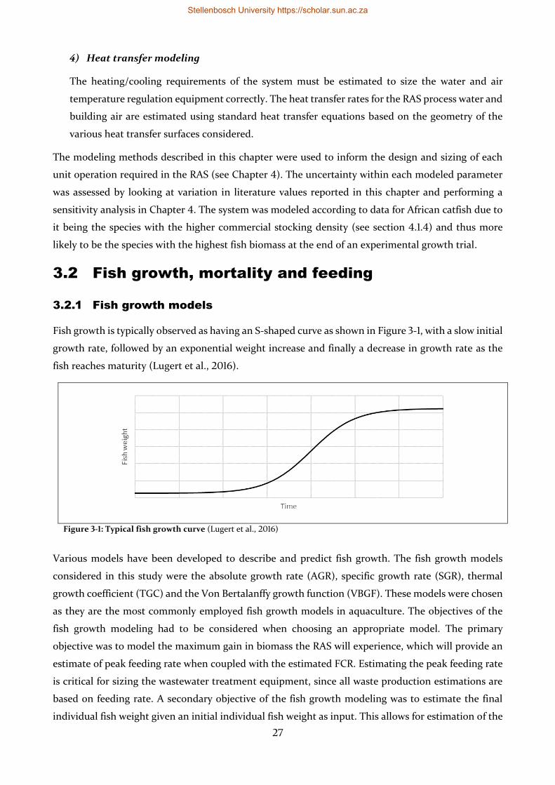
27

4) Heat transfer modeling

The heating/cooling requirements of the system must be estimated to size the water and air

temperature regulation equipment correctly. The heat transfer rates for the RAS process water and

building air are estimated using standard heat transfer equations based on the geometry of the

various heat transfer surfaces considered.

The modeling methods described in this chapter were used to inform the design and sizing of each

unit operation required in the RAS (see Chapter 4). The uncertainty within each modeled parameter

was assessed by looking at variation in literature values reported in this chapter and performing a

sensitivity analysis in Chapter 4. The system was modeled according to data for African catfish due to

it being the species with the higher commercial stocking density (see section 4.1.4) and thus more

likely to be the species with the highest fish biomass at the end of an experimental growth trial.

3.2 Fish growth, mortality and feeding

3.2.1 Fish growth models

Fish growth is typically observed as having an S-shaped curve as shown in Figure 3-1, with a slow initial

growth rate, followed by an exponential weight increase and finally a decrease in growth rate as the

fish reaches maturity (Lugert et al., 2016).

Figure 3-1: Typical fish growth curve (Lugert et al., 2016)

Various models have been developed to describe and predict fish growth. The fish growth models

considered in this study were the absolute growth rate (AGR), specific growth rate (SGR), thermal

growth coefficient (TGC) and the Von Bertalanffy growth function (VBGF). These models were chosen

as they are the most commonly employed fish growth models in aquaculture. The objectives of the

fish growth modeling had to be considered when choosing an appropriate model. The primary

objective was to model the maximum gain in biomass the RAS will experience, which will provide an

estimate of peak feeding rate when coupled with the estimated FCR. Estimating the peak feeding rate

is critical for sizing the wastewater treatment equipment, since all waste production estimations are

based on feeding rate. A secondary objective of the fish growth modeling was to estimate the final

individual fish weight given an initial individual fish weight as input. This allows for estimation of the


28

number of fish that need to be stocked at the start of the trial to roughly reach the target commercial

stocking density. Lugert et al. (2016) provided an excellent review of the considered fish growth

models.

3.2.1.1 Absolute growth rate

The absolute growth rate (AGR) model is shown in equation (3.1).

𝐴𝐺𝑅 =𝑤𝑡 − 𝑤𝑖

𝑡 (3.1)

where

𝐴𝐺𝑅 = Absolute growth rate [𝑔 𝑑𝑎𝑦⁄ ]

𝑤𝑡 = Fish body weight at time 𝑡 [𝑔]

𝑤𝑖 = Initial fish body weight [𝑔]

𝑡 = Production time [𝑑𝑎𝑦𝑠]

Thus, if the AGR is determined experimentally by solving equation (3.1), the fish growth curve of

weight vs time can be predicted.

𝑤𝑡 = 𝐴𝐺𝑅 ∙ 𝑡 + 𝑤𝑖 (3.2)

AGR is commonly used in experimental studies to compare treatments in a trial (Gericke, 2019;

Goosen, 2014; Oluwaseyi, 2016; Suresh and Lin, 1992). Although it is a valid tool for comparing

whether growth rates differ (e.g. in different experimental treatments in trials), it is a poor model of

fish growth and not an accurate model for prediction of fish body weight as equation (3.2) describes a

linear correlation. Lugert et al. (2016) found that the AGR model overestimated all intermediate fish

weights between the initial and final weights in their data set. An experimentally determined AGR

would be species and system specific.

3.2.1.2 Specific growth rate

The specific growth rate (SGR) model is shown in equation (3.3).

𝑆𝐺𝑅 =log (𝑤𝑡) − log (𝑤𝑖)

𝑡× 100 (3.3)

The SGR models the fish growth as a percentage increase in weight per day. As with the AGR, it is also

common in the comparison of treatments in experimental trials (Degani et al., 1989; Gericke, 2019;

Goosen, 2014; Pruszyński, 2003; Rahmatullah et al., 2010; Salhi et al., 2004; van de Nieuwegiessen et

al., 2008; Zhang et al., 2011). It has been suggested that SGR is suitable for prediction of the growth of

younger fish, which are still in the exponential growth phase, however growth over different life stages

is not well predicted. SGR was found to underestimate intermediate data whilst overestimating growth

at later life stages (Lugert et al., 2016). An experimentally determined SGR would also be species and

system specific.


29

3.2.1.3 Temperature growth coefficient

The temperature growth coefficient (TGC) model is given in equation (3.4).

𝑤𝑡 = (𝑤𝑖

1𝑏⁄

+ 𝑇𝐺𝐶 ∙ ∑ 𝑇𝑗

𝑡

𝑗=1

)

𝑏

(3.4)

where

𝑇𝐺𝐶 = Temperature growth coefficient [𝑔1 𝑏⁄ (℃ ∙ 𝑑𝑎𝑦)⁄ ]

𝑏 = Allometric exponent

𝑇𝑗 = Mean process water temperature at time step 𝑗 [℃]

The TGC model assumes that “growth rate is allometrically related to fish body weight” and “the

allometric constant of proportionality is directly related to mean daily water temperature averaged

over the rearing period” (Dumas et al., 2007). The allometric constants (𝑎 and 𝑏 in equation (3.5))

describe the relationship between fish length and body weight (Froese, 2006).

𝑤 = 𝑎 ∙ 𝑙𝑏 (3.5)

where

𝑤 = Fish body weight [𝑘𝑔]

𝑎 = Allometric constant [𝑘𝑔 𝑚⁄ ]


𝑙 = Fish length [𝑚]

Iwama and Tautz (1981) proposed an allometric exponent of 𝑏 = 3 for finfish. This assumption has

been verified experimentally for African catfish by Swanepoel (2017), and the TGC model has been

validated for warm-water fish (Bureau et al., 2000). Assuming the process water temperature in a RAS

is controlled at a constant value, equation (3.4) can be simplified to equation (3.6) (Lugert et al., 2016).

𝑤𝑡 = (𝑤𝑖

13⁄

+ 𝑇𝐺𝐶 ∙ 𝑇 ∙ 𝑡)3

(3.6)

Lugert et al. (2016) found the TGC model to fit their growth data better than both the AGR and SGR

models and propose it to be a suitable model for fish growth prediction from the early life stages to

the end of the exponential growth phase. The AGR and SGR models are only viable if the data is within

the exact life stage of the production being modeled (Lugert et al., 2016). Experimental data gathered

at water temperatures close to the desired temperature should be used to minimize errors in the

prediction (Dumas et al., 2010). It should be noted that the TGC model will overestimate the weight

of fish that are passing exponential growth. If the growth surpasses the exponential growth phase, a

non-linear growth model such as VBGF is needed to predict the S-shaped growth curve (Figure 3-1).


30

3.2.1.4 Von Bertalanffy growth function

The Von Bertalanffy growth function (VBGF) model is shown in equation (3.7).

𝑤𝑡 = 𝑤𝑖𝑛𝑓 ∙ (1 − 𝑒(−𝑘𝑉𝐵𝐺𝐹(𝑡−𝑡0)))𝑏 (3.7)

where

𝑤𝑖𝑛𝑓 = Asymptotic weight [𝑔]

𝑘𝑉𝐵𝐺𝐹 = Von Bertalanffy growth coefficient [1 𝑑𝑎𝑦⁄ ]

𝑡0 = Point where the curve intersects the x-axis [𝑑𝑎𝑦𝑠]


Assuming that the allometric exponent is constant, the VBGF model requires intermediate fish weight

data to regress the growth coefficient 𝑘, unlike the AGR, SGR and TGC models that only require the

initial and final fish weights. Although it was found to be the most accurate of the 4 growth models

(Lugert et al., 2016), there was a lack of reliable literature data and thus the VBGF model was not used.

However, the TGC model was deemed to be sufficiently accurate for this design and was used to model

fish growth.

3.2.2 Fish mortality model

Fish mortalities were modelled to calculate the correct number of fish to be stocked initially to reach

a target final fish biomass by accounting for fish mortalities during the experimental growth trial. Fish

mortality was modeled by Wik and Lindén (2004) as a first-order death process, accounting for the

higher amount of fish deaths observed at earlier stages of life. Number of fish (n) was modeled by

equation (3.8).

𝑛𝑡 = 𝑛𝑖 ∙ 𝑒−𝑘𝑑𝑒𝑎𝑡ℎ𝑡 (3.8)

where

𝑘𝑑𝑒𝑎𝑡ℎ = −1

𝑡𝑝ln (1 −

𝑝𝑛

100) [1 𝑑𝑎𝑦⁄ ]

𝑛𝑡 = Number of fish at time 𝑡

𝑛𝑖 = Initial number of fish

𝑡𝑝 = Length of production cycle of mortality data [𝑑𝑎𝑦𝑠]

𝑝𝑛 = Percentage of population that died in mortality data

A wide range of mortality rates have been observed in literature ranging from 6% to 50% for

production lengths of 30 days to 90 days (Akinwole and Faturoti, 2007; Gericke, 2019; Oluwaseyi,

2016). However, this parameter will not have much effect on the system design other than the

estimated number of fish that need to be stocked. An African catfish population in a typical trial at

Welgevallen grown from 9 – 304 g in 84 days had a mortality of 𝑝84 = 22% (Oluwaseyi, 2016, p. 85).

This resulted in an estimated 𝑘𝑑𝑒𝑎𝑡ℎ = 2.96 × 10−3 1

𝑑𝑎𝑦 .


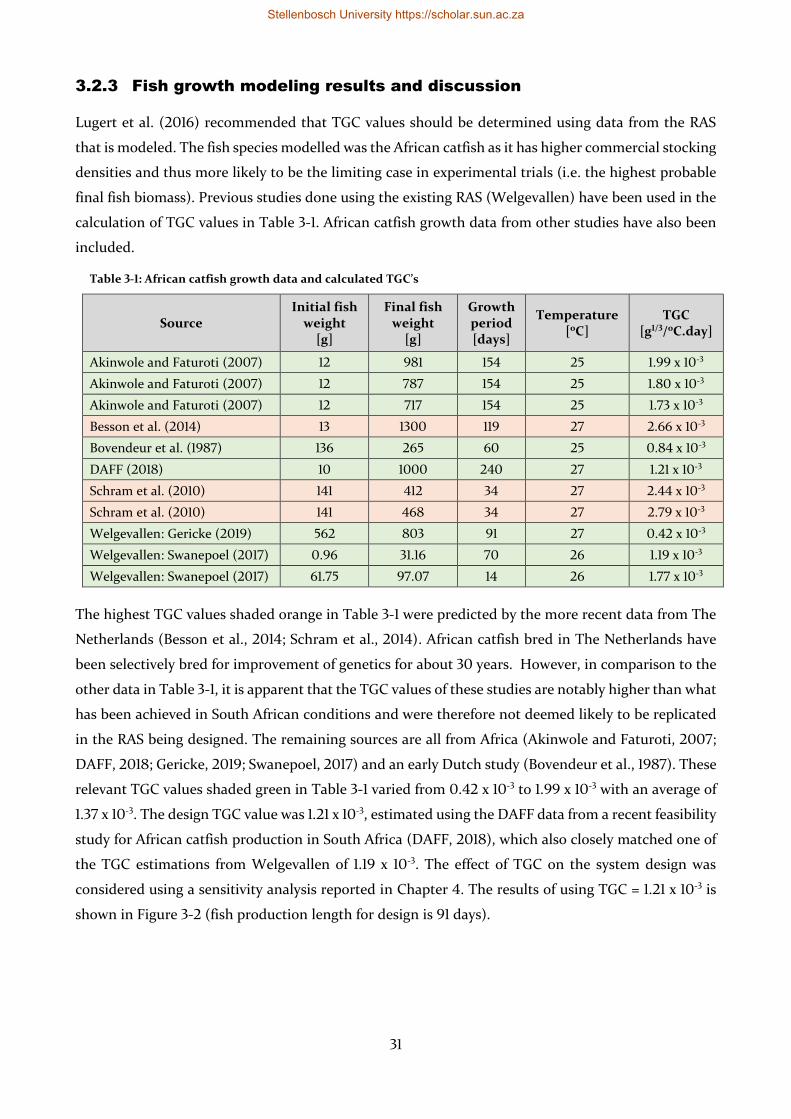
31

3.2.3 Fish growth modeling results and discussion

Lugert et al. (2016) recommended that TGC values should be determined using data from the RAS

that is modeled. The fish species modelled was the African catfish as it has higher commercial stocking

densities and thus more likely to be the limiting case in experimental trials (i.e. the highest probable

final fish biomass). Previous studies done using the existing RAS (Welgevallen) have been used in the

calculation of TGC values in Table 3-1. African catfish growth data from other studies have also been

included.

Table 3-1: African catfish growth data and calculated TGC’s

Source Initial fish

weight [g]

Final fish weight

[g]

Growth period [days]

Temperature [oC]

TGC [g1/3/oC.day]

Akinwole and Faturoti (2007) 12 981 154 25 1.99 x 10-3



Besson et al. (2014) 13 1300 119 27 2.66 x 10-3

Bovendeur et al. (1987) 136 265 60 25 0.84 x 10-3

DAFF (2018) 10 1000 240 27 1.21 x 10-3

Schram et al. (2010) 141 412 34 27 2.44 x 10-3

Schram et al. (2010) 141 468 34 27 2.79 x 10-3

Welgevallen: Gericke (2019) 562 803 91 27 0.42 x 10-3

Welgevallen: Swanepoel (2017) 0.96 31.16 70 26 1.19 x 10-3

Welgevallen: Swanepoel (2017) 61.75 97.07 14 26 1.77 x 10-3

The highest TGC values shaded orange in Table 3-1 were predicted by the more recent data from The

Netherlands (Besson et al., 2014; Schram et al., 2014). African catfish bred in The Netherlands have

been selectively bred for improvement of genetics for about 30 years. However, in comparison to the

other data in Table 3-1, it is apparent that the TGC values of these studies are notably higher than what

has been achieved in South African conditions and were therefore not deemed likely to be replicated

in the RAS being designed. The remaining sources are all from Africa (Akinwole and Faturoti, 2007;

DAFF, 2018; Gericke, 2019; Swanepoel, 2017) and an early Dutch study (Bovendeur et al., 1987). These

relevant TGC values shaded green in Table 3-1 varied from 0.42 x 10-3 to 1.99 x 10-3 with an average of

1.37 x 10-3. The design TGC value was 1.21 x 10-3, estimated using the DAFF data from a recent feasibility

study for African catfish production in South Africa (DAFF, 2018), which also closely matched one of

the TGC estimations from Welgevallen of 1.19 x 10-3. The effect of TGC on the system design was

considered using a sensitivity analysis reported in Chapter 4. The results of using TGC = 1.21 x 10-3 is

shown in Figure 3-2 (fish production length for design is 91 days).


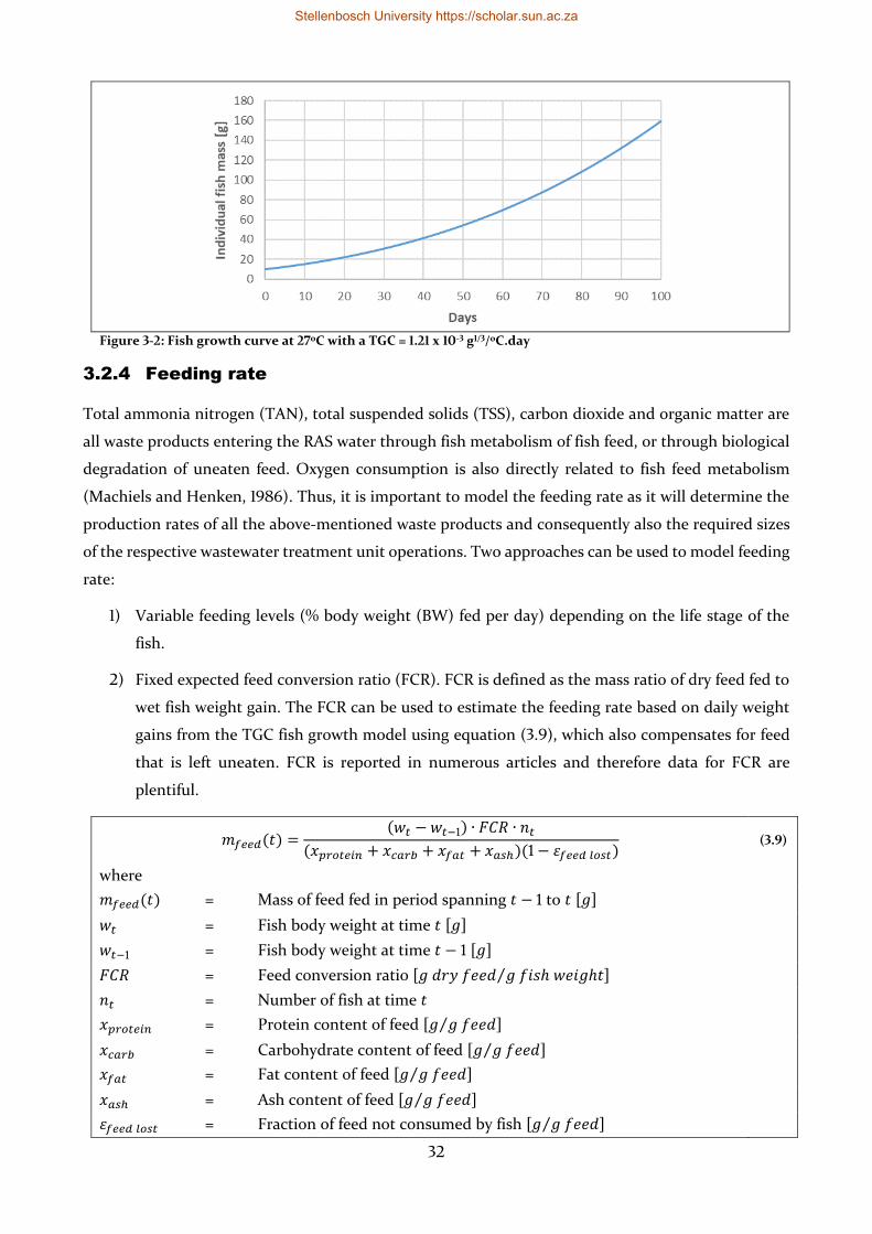
32

Figure 3-2: Fish growth curve at 27oC with a TGC = 1.21 x 10-3 g1/3/oC.day

3.2.4 Feeding rate

Total ammonia nitrogen (TAN), total suspended solids (TSS), carbon dioxide and organic matter are

all waste products entering the RAS water through fish metabolism of fish feed, or through biological

degradation of uneaten feed. Oxygen consumption is also directly related to fish feed metabolism

(Machiels and Henken, 1986). Thus, it is important to model the feeding rate as it will determine the

production rates of all the above-mentioned waste products and consequently also the required sizes

of the respective wastewater treatment unit operations. Two approaches can be used to model feeding

rate:

1) Variable feeding levels (% body weight (BW) fed per day) depending on the life stage of the

fish.

2) Fixed expected feed conversion ratio (FCR). FCR is defined as the mass ratio of dry feed fed to

wet fish weight gain. The FCR can be used to estimate the feeding rate based on daily weight

gains from the TGC fish growth model using equation (3.9), which also compensates for feed

that is left uneaten. FCR is reported in numerous articles and therefore data for FCR are

plentiful.

𝑚𝑓𝑒𝑒𝑑(𝑡) =(𝑤𝑡 − 𝑤𝑡−1) ∙ 𝐹𝐶𝑅 ∙ 𝑛𝑡

(𝑥𝑝𝑟𝑜𝑡𝑒𝑖𝑛 + 𝑥𝑐𝑎𝑟𝑏 + 𝑥𝑓𝑎𝑡 + 𝑥𝑎𝑠ℎ)(1 − 𝜀𝑓𝑒𝑒𝑑 𝑙𝑜𝑠𝑡) (3.9)

where

𝑚𝑓𝑒𝑒𝑑(𝑡) = Mass of feed fed in period spanning 𝑡 − 1 to 𝑡 [𝑔]

𝑤𝑡 = Fish body weight at time 𝑡 [𝑔]

𝑤𝑡−1 = Fish body weight at time 𝑡 − 1 [𝑔]

𝐹𝐶𝑅 = Feed conversion ratio [𝑔 𝑑𝑟𝑦 𝑓𝑒𝑒𝑑 𝑔 𝑓𝑖𝑠ℎ 𝑤𝑒𝑖𝑔ℎ𝑡⁄ ]

𝑛𝑡 = Number of fish at time 𝑡

𝑥𝑝𝑟𝑜𝑡𝑒𝑖𝑛 = Protein content of feed [𝑔 𝑔 𝑓𝑒𝑒𝑑⁄ ]

𝑥𝑐𝑎𝑟𝑏 = Carbohydrate content of feed [𝑔 𝑔 𝑓𝑒𝑒𝑑⁄ ]

𝑥𝑓𝑎𝑡 = Fat content of feed [𝑔 𝑔 𝑓𝑒𝑒𝑑⁄ ]

𝑥𝑎𝑠ℎ = Ash content of feed [𝑔 𝑔 𝑓𝑒𝑒𝑑⁄ ]

𝜀𝑓𝑒𝑒𝑑 𝑙𝑜𝑠𝑡 = Fraction of feed not consumed by fish [𝑔 𝑔 𝑓𝑒𝑒𝑑⁄ ]


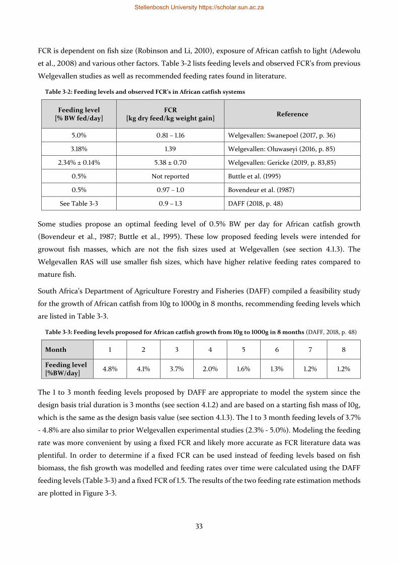
33

FCR is dependent on fish size (Robinson and Li, 2010), exposure of African catfish to light (Adewolu

et al., 2008) and various other factors. Table 3-2 lists feeding levels and observed FCR’s from previous

Welgevallen studies as well as recommended feeding rates found in literature.

Table 3-2: Feeding levels and observed FCR’s in African catfish systems

Feeding level [% BW fed/day]

FCR [kg dry feed/kg weight gain]

Reference

5.0% 0.81 – 1.16 Welgevallen: Swanepoel (2017, p. 36)

3.18% 1.39 Welgevallen: Oluwaseyi (2016, p. 85)

2.34% ± 0.14% 5.38 ± 0.70 Welgevallen: Gericke (2019, p. 83,85)

0.5% Not reported Buttle et al. (1995)

0.5% 0.97 – 1.0 Bovendeur et al. (1987)

See Table 3-3 0.9 – 1.3 DAFF (2018, p. 48)

Some studies propose an optimal feeding level of 0.5% BW per day for African catfish growth

(Bovendeur et al., 1987; Buttle et al., 1995). These low proposed feeding levels were intended for

growout fish masses, which are not the fish sizes used at Welgevallen (see section 4.1.3). The

Welgevallen RAS will use smaller fish sizes, which have higher relative feeding rates compared to

mature fish.

South Africa’s Department of Agriculture Forestry and Fisheries (DAFF) compiled a feasibility study

for the growth of African catfish from 10g to 1000g in 8 months, recommending feeding levels which

are listed in Table 3-3.

Table 3-3: Feeding levels proposed for African catfish growth from 10g to 1000g in 8 months (DAFF, 2018, p. 48)

Month 1 2 3 4 5 6 7 8

Feeding level [%BW/day]

4.8% 4.1% 3.7% 2.0% 1.6% 1.3% 1.2% 1.2%

The 1 to 3 month feeding levels proposed by DAFF are appropriate to model the system since the

design basis trial duration is 3 months (see section 4.1.2) and are based on a starting fish mass of 10g,

which is the same as the design basis value (see section 4.1.3). The 1 to 3 month feeding levels of 3.7%

- 4.8% are also similar to prior Welgevallen experimental studies (2.3% - 5.0%). Modeling the feeding

rate was more convenient by using a fixed FCR and likely more accurate as FCR literature data was

plentiful. In order to determine if a fixed FCR can be used instead of feeding levels based on fish

biomass, the fish growth was modelled and feeding rates over time were calculated using the DAFF

feeding levels (Table 3-3) and a fixed FCR of 1.5. The results of the two feeding rate estimation methods

are plotted in Figure 3-3.


34

Figure 3-3: Specific fish feeding rates estimated using DAFF feeding levels and FCR, both with TGC model estimated fish weights

There can be seen in Figure 3-3 that the fixed FCR model accurately matches the predicted feeding

rates of the DAFF feeding levels when using an FCR of 1.5. The step changes seen in the DAFF feeding

level feeding rates is due to changing feeding levels at a certain fish weight. An FCR of 1.5 is seen as a

conservative estimate of typical FCR’s observed in literature and equivalent to 3.3% BW per day during

peak loading and was thus used in the design for estimating the feeding rate.

3.3 Waste production models

3.3.1 TAN production

Ammonia is produced as a waste product from the breakdown of the protein contained in the fish

feed. The combined concentrations of ammonia and ammonium is expressed as total ammonia

nitrogen (TAN) (see section 2.1.3). Reported TAN production rates in literature are highly variable and

can differ by as much as a factor of 10 (Wheaton et al., 1994b). This is evidenced in observed TAN

production ratios of 3 – 7 g TAN/kg feed (Pruszyński, 2003), 38 – 81 g TAN/kg feed (Buttle et al., 1995),

40 g TAN/kg feed (Nijhof and Bovendeur, 1990) and 56 g TAN/kg feed (Bovendeur et al., 1987) in

African catfish culture. A rule of thumb used in industry for Atlantic salmon (Salmo salar) RAS is a

TAN production ratio of 35 – 45 kg TAN/kg feed (Gråkjær, 2019). Thus, care must be taken when sizing

equipment based on TAN production ratios from literature. This was done by doing a sensitivity

analysis (see section 4.5.4.3) to account for the uncertainty in the TAN production ratio.

As a starting design value for TAN production ratio, a theoretical estimation can be made. Essentially

all the nitrogen in the fish feed is contained in the proteins. A generally accepted assumption is that

the nitrogen content of protein is 0.16 grams N per gram protein (Besson et al., 2014; Mariotti et al.,


35

2008; Wik and Lindén, 2004). Since protein is the only significant source of nitrogen in fish feed, the

theoretical maximum TAN production can be calculated given the protein content of the feed. The

expected TAN production can be calculated by subtracting the expected nitrogen retention (NR) of

the fish (g N retained in fish/g N in consumed feed) from the theoretical maximum TAN production.

Observed levels of NR in African catfish has been reported in literature as 31% (Farhat and Khan, 2011),

34 – 38% (van Weerd et al., 2003), 37 – 38% (Torreele et al., 1993) and 42% (Lim et al., 2001). Trials

done with black catfish (Rhamdia quelen) resulted in NRs of 32 – 40%. Possible reasons for these

differences in observed NR’s are that (1) the life stages and hence the digestive capabilities of the fish

and the feed formulations differed between the studies and (2) uneaten feed can skew the results of a

study due to the difficulty of measuring uneaten feed mass, which must be accounted for when

calculating NR. A lower NR will result in more nitrogen being excreted by the fish, increasing TAN

production. An average nitrogen retention of 35% was chosen to model the RAS.

The typical protein contents of commercial and experimental fish feed are listed in Table 3-4. The

information in Table 3-4 shows the protein contents vary from around 40% to 50%. An average of

45% protein content was chosen to model the RAS. The conservative upper value was not chosen due

to the design including a sensitivity analysis on the design parameters, which will account for

conservative estimates.

Table 3-4: Protein content of fish feeds in literature

Fish species Protein content % [g protein/g feed]

Source

African catfish

45% Besson et al. (2014)

47.1% Bovendeur et al. (1987)

45% Akinwole and Faturoti (2007)

49% Schram et al. (2010)

36.9 – 38.4% Swanepoel (2017, p. 43)

37% Gericke (2019, p. 117)

41% Talamuk (2016, p. 27)

41 – 50% Buttle et al. (1995)

44% Palm et al. (2018)

Atlantic salmon 44% Wik and Lindén (2004)

Mozambique tilapia 40 – 45% Goosen (2014, pp. 56, 93)

The excreted nitrogen is in two forms namely urine and feces. The nitrogen in the urine is regarded as

TAN directly excreted into the process water, while the nitrogen in the feces slowly diffuses into the

water over time. Buttle et al. (1995) found that 80% of the excreted nitrogen enters the water as TAN.

For the purposes of this model, a conservative estimate is taken by assuming that 100% of the excreted

nitrogen enters the water immediately as TAN.

As the above described methodology would suggest, TAN production ratio (grams TAN produced per

gram feed fed) is a function of feed protein content, nitrogen content of protein, nitrogen retention in

the fish and mass of feed fed. The TAN production ratio model is given in Equation (3.10).


36


= 𝑚𝑓𝑒𝑒𝑑 × 𝐶𝑝𝑟𝑜𝑡𝑒𝑖𝑛 × 𝐶𝑁,𝑝𝑟𝑜𝑡𝑒𝑖𝑛 × (1 − 𝑁𝑅) (3.10)

where


= Total ammonia-nitrogen added to water [𝑔 𝑁 𝑑𝑎𝑦⁄ ]

𝑚𝑓𝑒𝑒𝑑 = Feeding rate [𝑔 𝑓𝑒𝑒𝑑 𝑑𝑎𝑦⁄ ]

𝐶𝑝𝑟𝑜𝑡𝑒𝑖𝑛 = Feed protein content [𝑔 𝑝𝑟𝑜𝑡𝑒𝑖𝑛 𝑔 𝑓𝑒𝑒𝑑⁄ ]

𝐶𝑁,𝑝𝑟𝑜𝑡𝑒𝑖𝑛 = Nitrogen content of protein [𝑔 𝑁 𝑔 𝑝𝑟𝑜𝑡𝑒𝑖𝑛⁄ ]

𝑁𝑅 = Nitrogen retention in the fish [𝑔 𝑁 𝑟𝑒𝑡𝑎𝑖𝑛𝑒𝑑 𝑔 𝑁 𝑖𝑛𝑡𝑎𝑘𝑒⁄ ]

Given the assumptions of 𝐶𝑝𝑟𝑜𝑡𝑒𝑖𝑛 = 45%, 𝐶𝑁,𝑝𝑟𝑜𝑡𝑒𝑖𝑛 = 0.16, and 𝑁𝑅 = 35%, the TAN production ratio

was calculated as (𝑚𝑝𝑟𝑜𝑑)

𝑇𝐴𝑁

𝑚𝑓𝑒𝑒𝑑= 0.047

𝑔 𝑇𝐴𝑁

𝑔 𝑓𝑒𝑒𝑑

3.3.2 Oxygen consumption and carbon dioxide production

Dissolved oxygen in a RAS is consumed by fish, autotrophic bacteria and heterotrophic bacteria, which

all need to be estimated in order to size the aeration system correctly. Oxygen consumption in the fish

tanks is mainly through fish respiration with oxygen consumption due to bacterial growth being

negligible. A rule of thumb for oxygen consumption by fish respiration has been proposed where 0.25

kg O2 is consumed per kg of feed consumed by the fish (Timmons and Ebeling, 2007, p. 87). This

estimate is supported by similar findings for African catfish ranging between 0.235 – 0.255 kg O2/kg

feed (Bovendeur et al., 1987; Machiels and Henken, 1986).

Oxygen in the biofilter water is consumed by both autotrophic and heterotrophic bacteria.

Autotrophic bacteria consume oxygen during nitrification. The stoichiometry of the oxidation of

ammonia to nitrate with nitrite as intermediate results in 4.25 g O2 consumed per g TAN converted

(Eding et al., 2006; Losordo and Westers, 1994). Heterotrophic bacteria consume oxygen when

breaking down organics. General design guidelines are proposed to be between 0.13 – 0.50 kg O2 per

kg of feed fed (Timmons and Ebeling, 2007, p. 87). However, a more accurate estimation was done by

modeling the organic matter production rates (see section 3.3.4).

Dissolved carbon dioxide is produced by fish respiration with 1 mol CO2 produced per 1 mol O2

consumed. Converting to a mass basis yields a ratio of 1.375 g CO2/g O2 (Timmons and Ebeling, 2007;

Wik et al., 2009). A similar ratio of 1.27 g CO2/g O2 was found experimentally (Bovendeur et al., 1987).

It was decided to use the higher value of 1.375 g CO2/g O2 to model the RAS. Dissolved carbon dioxide

is also produced by heterotrophic bacterial aerobic digestion of organic carbon matter. This is

produced in the same ratio as above (Gallert and Winter, 2008).

3.3.3 Total suspended solids production

Feces and uneaten feed are the main sources of TSS in water. Various levels of TSS production have

been observed in literature, all being reported as a percentage of the dry feed mass being converted to


37

TSS. A general rule of thumb where 25% of the dry feed mass is converted to TSS has been proposed

(Timmons and Ebeling, 2007, p. 87). Studies on channel catfish (Ictalurus punctatus) have found

varying results, with one study finding 18% of dry feed mass converted to TSS whilst another found

that 43% was converted. Studies on salmonids have found that 25 – 30% of the dry feed is converted

to TSS (Chen et al., 1994, pp. 62–63). A 20% conversion of dry feed to TSS was estimated as the TSS

production rate in a rainbow trout (Oncorhynchus mykiss) system (Lekang, 2007, p. 58).

Based on the above literature observations, it was concluded that the rule of thumb where 25% of the

dry feed is converted to TSS is a reasonable average design value assumption given that a sensitivity

analysis was done to account for more conservative values.

3.3.4 Particulate and dissolved organic matter

Organic matter is excreted by fish in particulate and dissolved form. This organic matter contributes

to the BOD5 within the system, which negatively affects nitrification rates (Eding et al., 2006).

Therefore, the overall BOD5 production rate within the system needed to be modeled.

Bovendeur et al. (1987, p. 351) found that the distribution of excreted organic matter in a typical

African catfish RAS was 65% particulate organic matter (POM) and 35% dissolved organic matter

(DOM). This can also be expressed as a DOM to POM ratio of 0.54: 1. Another study found that almost

all organic matter in a rainbow trout (Oncorhynchus mykiss) RAS was dissolved (Rojas-Tirado et al.,

2017). They did not include particles removed in solids removal steps though. Bovendeur et al. (1987,

p. 351) was the only literature source found that reports the excreted distribution of organic matter.

For this study, it was assumed that all excreted TSS will be organic matter. The POM production can

then be regarded to be equal to TSS production. DOM production can then be calculated using the

assumed DOM to POM ratio of 0.54: 1. Bovendeur et al. (1987, p. 335) found African catfish waste

organic matter to have a COD to organic matter (POM + DOM) ratio of 1.4: 1, and a biodegradability

(BOD/COD) of 80%. Additional data for COD and BOD5 originating from African catfish excreted

organic matter were not available to the knowledge of the author. Estimation of BOD5 was done by

calculating the COD of the organic matter (POM + DOM) using the 1.4: 1 ratio and assuming 80% of

that will be BOD5.


38

3.4 Biofiltration modeling

Two types of biofilters were modeled in this design. A tricking filter was modeled to determine

whether it is necessary to replace the current trickling filters based on the TAN removal capacity of

the current system. A moving bed bioreactor (MBBR) was modeled for the purpose of replacing the

existing tricking filters with MBBRs. Described in this section are the various approaches considered

for modeling trickling filters and MBBRs. Eventually trickling filter model approach 4 (plug-flow

model) and MBBR model approach 2 was used in the design.

3.4.1 Trickling filter model approach 1: Well-mixed reactor models

Trickling filters have been modeled as a continuously stirred-tank reactor (CSTR), which assumes that

the reactor is well-mixed (Bovendeur et al., 1987; Lastiri et al., 2018). In other words, the concentration

of the reactant (ammonia in this case) is the same everywhere inside the reactor. This assumption

would mean that the TAN concentration exiting the trickling filter at the bottom of the reactor is the

same as the TAN concentration near the top of the column. However, a trickling filter cannot be

modeled as a CSTR due to the TAN concentration clearly decreasing as the water flows through the

column. This is supported by experiments done by Nijhof (1995). Therefore, this approach was not

considered further.

3.4.2 Trickling filter model approach 2: System specific empirical data

Liao and Mayo (1974) proposed an empirical approach to determine the TAN removal rate in trickling

filters based on experimental data. However, this model is only applicable to specific trickling filter

systems with Koch rings as packing, hydraulic loadings ranging from 86.4 – 147 m3/m2.day and TAN

concentrations ≤ 1 mg/L. This would not be applicable to the proposed RAS which has a TAN limit

ranging up to 3 mg/L, or the current existing trickling filter, which has structured packing.

Manufacturers of various biofilters use experience based estimates for the TAN removal rate (Drennan

et al., 2006). These estimates are only valid for applications with a specific fish species, water quality

conditions and system configuration (Eding et al., 2006). The system specific empirical approaches

were thus not further considered to model a trickling filter.

3.4.3 Trickling filter model approach 3: Activated sludge model

Wik (1999) took a more complex approach to modeling trickling filters by using the activated sludge

models (ASM) of Henze et al. (1987). The activated sludge models dynamically predict the following:

• Bacterial growth – Both autotrophs and heterotrophs.

• Utilization of oxygen.

• Consumption of ammonia and organic matter.

• Diffusion of substrates from the bulk fluid into the biofilm and vice versa.

• Diffusion of substrates within the biofilm.


39

Although this model provides good predictive capability, it is complex and requires estimates for a

large number of parameters and it is unclear whether estimates generated through this method hold

significant advantage over simpler models. For the purposes of this design, a simpler model which

delivers sufficiently accurate biofiltration estimates, but which is less complex, was preferred to assess

the capacity of the trickling filters in the current system.

3.4.4 Trickling filter model approach 4: Plug-flow model

A plug flow model proposed by Nijhof (1995) predicts nitrification rates using TAN concentration,

hydraulic surface loading and trickling filter height and model parameter as model inputs. Due to the

simplicity of the model and applicability to the system being modeled, this model was chosen to assess

the capacity of the existing trickling filters in the system.

The nitrification reaction kinetics used in the model by Nijhof (1995) are half-order/zero-order

kinetics, which are commonly used to model biofilters (Eding et al., 2006). The main ways that the

nitrification rate can be limited or impacted in this kinetic model are:

1) Limited by TAN concentration – TAN diffusion limitation (Case 1 in Table 3-5)

2) Limited by oxygen concentration – Oxygen diffusion limitation (Case 2 in Table 3-5)

3) Limited by intrinsic reaction rate – Reaction rate limited (Case 3 in Table 3-5)

Transition concentrations for TAN and oxygen where reaction kinetics change from zero-order to half-

order are defined as 𝐶𝑇𝐴𝑁∗ and 𝐶𝑂2

∗. If the actual substrate concentration is above its respective

transition concentration, the nitrification rate cannot be limited by the respective substrate. If both

substrates are in abundance, the nitrification rate is limited by the intrinsic reaction rate of the

nitrification reaction. The TAN diffusion limitation case was modeled as half-order kinetics with

model parameters 𝑎1 and 𝑎2 (Equation (3.11)) and oxygen diffusion limitation as zero-order kinetics

with model parameter 𝑎3 (Equation (3.12)). Studies done in freshwater RAS have consistently found

that the ratio of the transition concentrations (𝐶𝑂2

∗ 𝐶𝑇𝐴𝑁∗⁄ ) range between 3.4 and 3.8 (Bovendeur et

al., 1987; Bovendeur and Klapwijk, 1986; Nijhof and Bovendeur, 1990).


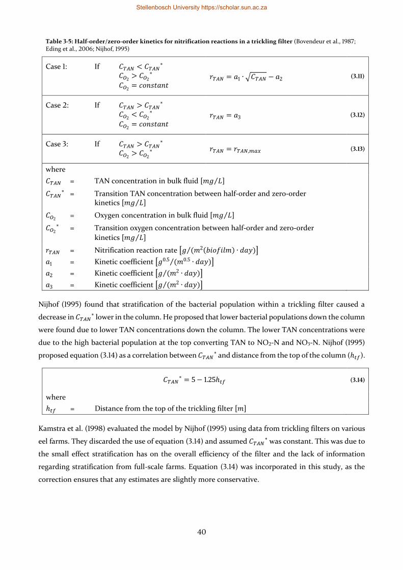
40

Table 3-5: Half-order/zero-order kinetics for nitrification reactions in a trickling filter (Bovendeur et al., 1987; Eding et al., 2006; Nijhof, 1995)

Case 1: If 𝐶𝑇𝐴𝑁 < 𝐶𝑇𝐴𝑁∗

𝐶𝑂2> 𝐶𝑂2

∗

𝐶𝑂2= 𝑐𝑜𝑛𝑠𝑡𝑎𝑛𝑡

𝑟𝑇𝐴𝑁 = 𝑎1 ∙ √𝐶𝑇𝐴𝑁 − 𝑎2 (3.11)

Case 2: If 𝐶𝑇𝐴𝑁 > 𝐶𝑇𝐴𝑁∗

𝐶𝑂2< 𝐶𝑂2

∗

𝐶𝑂2= 𝑐𝑜𝑛𝑠𝑡𝑎𝑛𝑡

𝑟𝑇𝐴𝑁 = 𝑎3 (3.12)

Case 3: If 𝐶𝑇𝐴𝑁 > 𝐶𝑇𝐴𝑁∗

𝐶𝑂2> 𝐶𝑂2

∗ 𝑟𝑇𝐴𝑁 = 𝑟𝑇𝐴𝑁,𝑚𝑎𝑥 (3.13)

where

𝐶𝑇𝐴𝑁 = TAN concentration in bulk fluid [𝑚𝑔 𝐿⁄ ]

𝐶𝑇𝐴𝑁∗ = Transition TAN concentration between half-order and zero-order

kinetics [𝑚𝑔 𝐿⁄ ]

𝐶𝑂2 = Oxygen concentration in bulk fluid [𝑚𝑔 𝐿⁄ ]

𝐶𝑂2

∗ = Transition oxygen concentration between half-order and zero-order

kinetics [𝑚𝑔 𝐿⁄ ]

𝑟𝑇𝐴𝑁 = Nitrification reaction rate [𝑔 (𝑚2(𝑏𝑖𝑜𝑓𝑖𝑙𝑚) ∙ 𝑑𝑎𝑦)⁄ ]

𝑎1 = Kinetic coefficient [𝑔0.5 (𝑚0.5 ∙ 𝑑𝑎𝑦)⁄ ]

𝑎2 = Kinetic coefficient [𝑔 (𝑚2 ∙ 𝑑𝑎𝑦)⁄ ]

𝑎3 = Kinetic coefficient [𝑔 (𝑚2 ∙ 𝑑𝑎𝑦)⁄ ]

Nijhof (1995) found that stratification of the bacterial population within a trickling filter caused a

decrease in 𝐶𝑇𝐴𝑁∗ lower in the column. He proposed that lower bacterial populations down the column

were found due to lower TAN concentrations down the column. The lower TAN concentrations were

due to the high bacterial population at the top converting TAN to NO2-N and NO3-N. Nijhof (1995)

proposed equation (3.14) as a correlation between 𝐶𝑇𝐴𝑁∗ and distance from the top of the column (ℎ𝑡𝑓).

𝐶𝑇𝐴𝑁∗ = 5 − 1.25ℎ𝑡𝑓 (3.14)

where

ℎ𝑡𝑓 = Distance from the top of the trickling filter [𝑚]

Kamstra et al. (1998) evaluated the model by Nijhof (1995) using data from trickling filters on various

eel farms. They discarded the use of equation (3.14) and assumed 𝐶𝑇𝐴𝑁∗ was constant. This was due to

the small effect stratification has on the overall efficiency of the filter and the lack of information

regarding stratification from full-scale farms. Equation (3.14) was incorporated in this study, as the

correction ensures that any estimates are slightly more conservative.


41

3.4.4.1 Case 1: TAN diffusion limitation

For this case, the trickling filter was assumed to operate under TAN diffusion limitation conditions if

𝐶𝑇𝐴𝑁 < 𝐶𝑇𝐴𝑁∗. Nijhof (1995) proposed a correlation between the half-order nitrification rate coefficient

𝑎 in equation (3.11) and the hydraulic surface loading rate (HSL) of the trickling filter. This correlation

is given in equation (3.15). The second kinetic coefficient 𝑏 was regressed as a constant of 𝑎2 =

0.1 𝑔 (𝑚2 ∙ 𝑑𝑎𝑦)⁄ .

𝑎1 = 7.81 × 10−4𝐻𝑆𝐿 + 0.261 (3.15)

where

𝐻𝑆𝐿 = Hydraulic surface loading rate [𝑚3 (𝑚2 ∙ 𝑑𝑎𝑦)⁄ ]

The HSL is calculated by dividing the recirculating flow rate by the cross-sectional area of the trickling

filter. A minimum HSL is required to keep the biofilm surface area wet, but this does not determine

the minimum HSL. Clogging can occur when solids attach to the biofilm and buildup occurs with

insufficient scouring of the biofilm. Therefore, it is recommended that HSL must be kept above 300

m3/m2.day to prevent clogging of the filter (Eding et al., 2006). Within the proposed model (equation

(3.15)), the high and low values of HSL will overestimate and underestimate the nitrification rate

respectively. Greiner and Timmons (1998) tested hydraulic loading rates in a trickling filter ranging

from 469 to 1231 m3/(m2.day) and found no increase in nitrification rates. This suggests that there is

an upper limit above which hydraulic loading rates have no further effect on nitrification rates.

Equation (3.15) was regressed from data collected at HSLs of 75, 150 and 300 m3/m2.day (Nijhof, 1995).

Since HSLs higher than 300 m3/m2.day are recommended to prevent clogging, the desired HSL would

be higher than the range investigated when the model parameters were regressed, which introduces

the possibility of nitrification rates being overestimated by the model.

3.4.4.2 Case 2: Oxygen diffusion limitation

The trickling filter was assumed to operate under oxygen diffusion limitation conditions if 𝐶𝑇𝐴𝑁 >

𝐶𝑇𝐴𝑁∗. This would result in a zero-order nitrification rate with respect to TAN concentration and is

determined by the oxygen concentration. The oxygen concentrations used in the study by Nijhof

(1995) varied from 7.4 – 8.2 mg/L., The TAN concentration did not fall below the zero-order transition

TAN concentration during the modeling of the trickling filters (see section 4.5.1). Thus, the zero-order

nitrification rate and bulk water oxygen concentration in the trickling filters was not estimated in this

study.

Oxygen diffusion limitation could exist if the BOD5 from organic matter in the water was sufficiently

high. Nitrification can only occur if the BOD5 < 110 mg/L and is due to heterotrophic bacteria

overgrowing the autotrophic bacteria when there is a high organic carbon concentration in the water

(Gallert and Winter, 2008). A 30% reduction of nitrification rates in submerged filters due to organic

loading has been observed in literature (Zhu and Chen, 2001). The effect of BOD5 on trickling filter

performance was not modeled and is motivated in section 4.5.1.


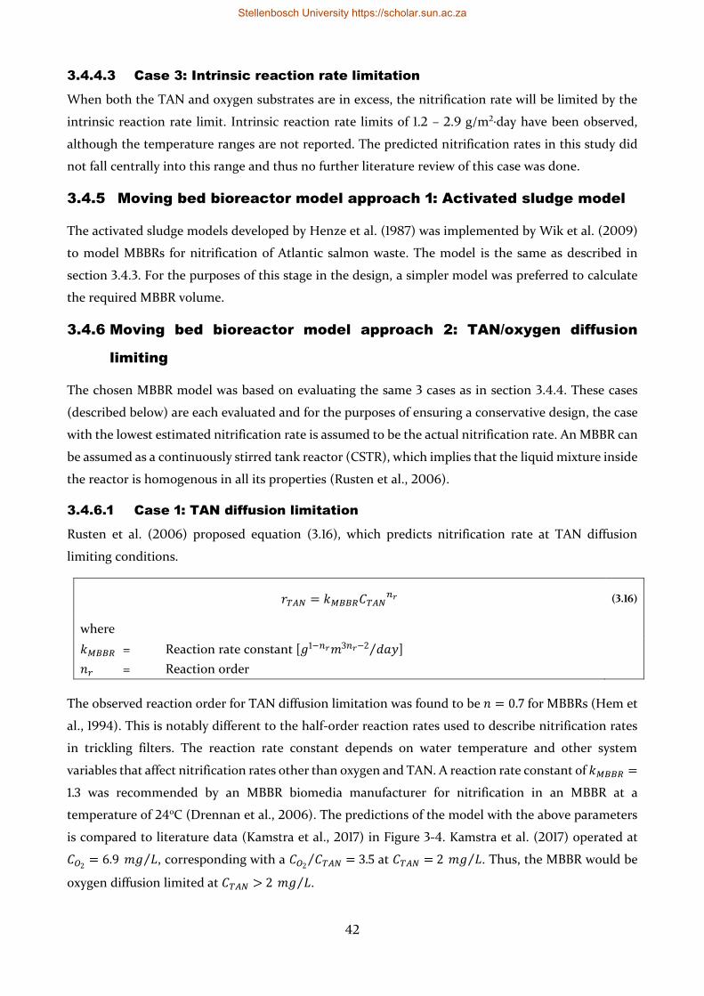
42

3.4.4.3 Case 3: Intrinsic reaction rate limitation

When both the TAN and oxygen substrates are in excess, the nitrification rate will be limited by the

intrinsic reaction rate limit. Intrinsic reaction rate limits of 1.2 – 2.9 g/m2∙day have been observed,

although the temperature ranges are not reported. The predicted nitrification rates in this study did

not fall centrally into this range and thus no further literature review of this case was done.

3.4.5 Moving bed bioreactor model approach 1: Activated sludge model

The activated sludge models developed by Henze et al. (1987) was implemented by Wik et al. (2009)

to model MBBRs for nitrification of Atlantic salmon waste. The model is the same as described in

section 3.4.3. For the purposes of this stage in the design, a simpler model was preferred to calculate

the required MBBR volume.

3.4.6 Moving bed bioreactor model approach 2: TAN/oxygen diffusion

limiting

The chosen MBBR model was based on evaluating the same 3 cases as in section 3.4.4. These cases

(described below) are each evaluated and for the purposes of ensuring a conservative design, the case

with the lowest estimated nitrification rate is assumed to be the actual nitrification rate. An MBBR can

be assumed as a continuously stirred tank reactor (CSTR), which implies that the liquid mixture inside

the reactor is homogenous in all its properties (Rusten et al., 2006).

3.4.6.1 Case 1: TAN diffusion limitation

Rusten et al. (2006) proposed equation (3.16), which predicts nitrification rate at TAN diffusion

limiting conditions.

𝑟𝑇𝐴𝑁 = 𝑘𝑀𝐵𝐵𝑅𝐶𝑇𝐴𝑁𝑛𝑟 (3.16)

where

𝑘𝑀𝐵𝐵𝑅 = Reaction rate constant [𝑔1−𝑛𝑟𝑚3𝑛𝑟−2 𝑑𝑎𝑦⁄ ]

𝑛𝑟 = Reaction order

The observed reaction order for TAN diffusion limitation was found to be 𝑛 = 0.7 for MBBRs (Hem et

al., 1994). This is notably different to the half-order reaction rates used to describe nitrification rates

in trickling filters. The reaction rate constant depends on water temperature and other system

variables that affect nitrification rates other than oxygen and TAN. A reaction rate constant of 𝑘𝑀𝐵𝐵𝑅 =

1.3 was recommended by an MBBR biomedia manufacturer for nitrification in an MBBR at a

temperature of 24oC (Drennan et al., 2006). The predictions of the model with the above parameters

is compared to literature data (Kamstra et al., 2017) in Figure 3-4. Kamstra et al. (2017) operated at

𝐶𝑂2= 6.9 𝑚𝑔 𝐿⁄ , corresponding with a 𝐶𝑂2

𝐶𝑇𝐴𝑁⁄ = 3.5 at 𝐶𝑇𝐴𝑁 = 2 𝑚𝑔 𝐿⁄ . Thus, the MBBR would be

oxygen diffusion limited at 𝐶𝑇𝐴𝑁 > 2 𝑚𝑔 𝐿⁄ .


43

Figure 3-4: Nitrification rates observed in literature compared to the TAN diffusion limiting model equation (3.16)

Half-order kinetics (𝑛𝑟 = 0.5) describes the variation in literature data overall better than 𝑛𝑟 = 0.7,

with R-squared values of 0.93 and 0.82 respectively. This is due to the overestimation of nitrification

rates at 𝐶𝑇𝐴𝑁 > 1.3 𝑚𝑔 𝐿⁄ when using 𝑛𝑟 = 0.7. The estimated MBBR outflow TAN concentration and

also the internal TAN concentration due to the CSTR assumption in this study was 𝐶𝑇𝐴𝑁 < 0.4 𝑚𝑔 𝐿⁄ ,

where both 𝑛𝑟 = 0.5 and 𝑛𝑟 = 0.7 provides similar estimations of nitrification rates. Therefore, the

MBBR specifically derived reaction order of 𝑛𝑟 = 0.7 was used in the design.

3.4.6.2 Case 2: Oxygen diffusion limitation

Increased organic loading on the biofilm causes growth of heterotrophic bacteria in the outer biofilm

layer. This decreases the effective oxygen concentration in the biofilm that is available for nitrifying

bacteria, decreasing the nitrification rate (Rusten et al., 2006). A study quantified this oxygen

concentration decrease as 0.5 mg/L at low organic loadings and 2.5 mg/L at 1.5 g BOD5/m2∙day (Rusten

et al., 1995). Instead of modeling the decrease in oxygen concentration in the biofilm, it was more

convenient to use empirical data (Table 3-6) of nitrification rates observed at different bulk water

oxygen concentrations and organic loadings (Hem et al., 1994).

𝑅2 = 0.82

𝑅2 = 0.93


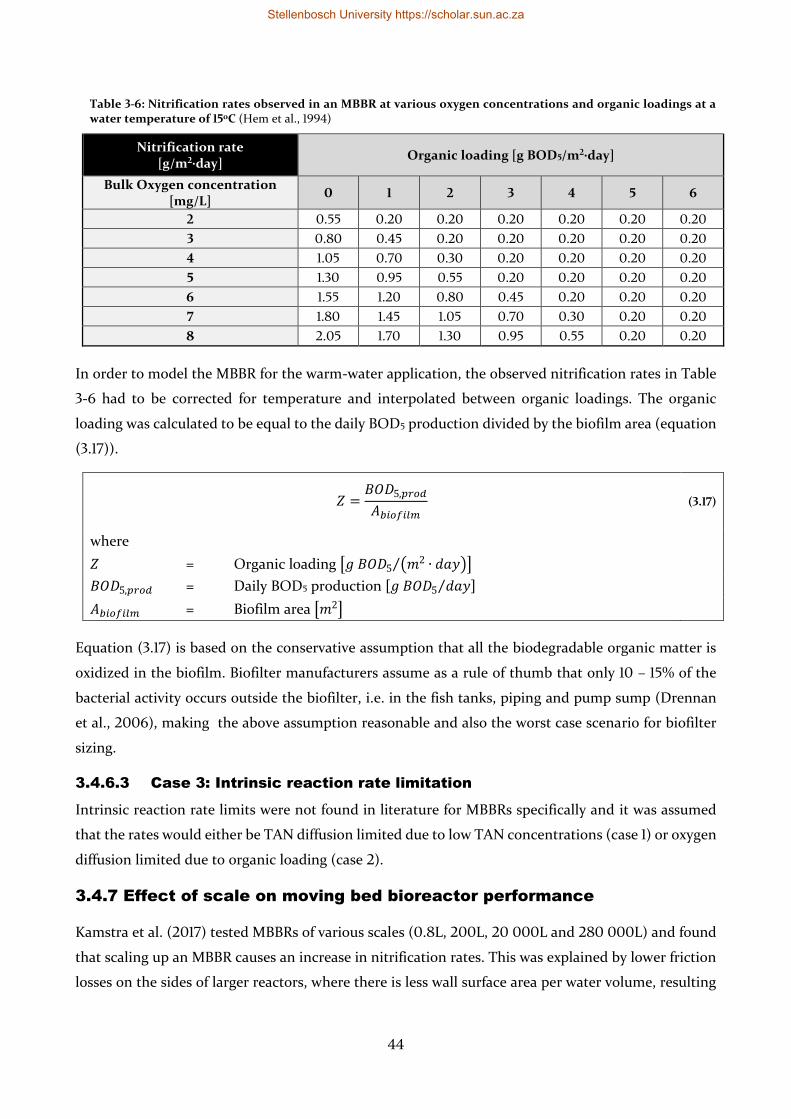
44

Table 3-6: Nitrification rates observed in an MBBR at various oxygen concentrations and organic loadings at a water temperature of 15oC (Hem et al., 1994)

Nitrification rate [g/m2∙day]

Organic loading [g BOD5/m2∙day]

Bulk Oxygen concentration [mg/L]

0 1 2 3 4 5 6

2 0.55 0.20 0.20 0.20 0.20 0.20 0.20

3 0.80 0.45 0.20 0.20 0.20 0.20 0.20

4 1.05 0.70 0.30 0.20 0.20 0.20 0.20

5 1.30 0.95 0.55 0.20 0.20 0.20 0.20

6 1.55 1.20 0.80 0.45 0.20 0.20 0.20

7 1.80 1.45 1.05 0.70 0.30 0.20 0.20

8 2.05 1.70 1.30 0.95 0.55 0.20 0.20

In order to model the MBBR for the warm-water application, the observed nitrification rates in Table

3-6 had to be corrected for temperature and interpolated between organic loadings. The organic

loading was calculated to be equal to the daily BOD5 production divided by the biofilm area (equation

(3.17)).

𝑍 =𝐵𝑂𝐷5,𝑝𝑟𝑜𝑑

𝐴𝑏𝑖𝑜𝑓𝑖𝑙𝑚 (3.17)

where

𝑍 = Organic loading [𝑔 𝐵𝑂𝐷5 (𝑚2 ∙ 𝑑𝑎𝑦)⁄ ]

𝐵𝑂𝐷5,𝑝𝑟𝑜𝑑 = Daily BOD5 production [𝑔 𝐵𝑂𝐷5 𝑑𝑎𝑦⁄ ]

𝐴𝑏𝑖𝑜𝑓𝑖𝑙𝑚 = Biofilm area [𝑚2]

Equation (3.17) is based on the conservative assumption that all the biodegradable organic matter is

oxidized in the biofilm. Biofilter manufacturers assume as a rule of thumb that only 10 – 15% of the

bacterial activity occurs outside the biofilter, i.e. in the fish tanks, piping and pump sump (Drennan

et al., 2006), making the above assumption reasonable and also the worst case scenario for biofilter

sizing.

3.4.6.3 Case 3: Intrinsic reaction rate limitation

Intrinsic reaction rate limits were not found in literature for MBBRs specifically and it was assumed

that the rates would either be TAN diffusion limited due to low TAN concentrations (case 1) or oxygen

diffusion limited due to organic loading (case 2).

3.4.7 Effect of scale on moving bed bioreactor performance

Kamstra et al. (2017) tested MBBRs of various scales (0.8L, 200L, 20 000L and 280 000L) and found

that scaling up an MBBR causes an increase in nitrification rates. This was explained by lower friction

losses on the sides of larger reactors, where there is less wall surface area per water volume, resulting


45

in more turbulence. They found the 0.8L MBBR to have a nitrification rate 20% lower than the 200L

MBBR. However, no model was proposed to predict these effects and was not considered in this study.

3.4.8 Effect of temperature on nitrification

The nitrification rates of the biofilter models needed to be corrected for temperature due to higher

reaction rates being observed at higher temperatures. This was done using the following equation

(Eding et al., 2006; Rusten et al., 2006):

𝑟𝑇2= 𝑟𝑇1

𝜃(𝑇2−𝑇1) (3.18)

where

𝑟𝑇1 = Reaction rate at water temperature 1 [𝑔 (𝑚2 ∙ 𝑑𝑎𝑦)⁄ ]

𝑟𝑇1 = Reaction rate at water temperature 2 [𝑔 (𝑚2 ∙ 𝑑𝑎𝑦)⁄ ]

𝑇1 = Water temperature of system 1 [℃]

𝑇2 = Water temperature of system 2 [℃]

𝜃 = Temperature activity coefficient

Observed values for 𝜃 in trickling filters range from 1.02 to 1.08 (Eding et al., 2006). Rusten et al.

(1995) found a 𝜃 value of 1.09 to describe temperature variations in nitrification rates in MBBRs.

Kinyage and Pedersen (2016) found a 𝜃 value of 1.079 to be valid for MBBRs at temperatures ranging

from 6 – 30oC. Bovendeur et al. (1987) regressed a 𝜃 value of 1.08 from trickling filter data when rearing

African catfish at 25oC, and consequently a 𝜃 value of 1.08 was also used for this design. The effect of

lower temperature activity coefficients is investigated in a sensitivity analysis (see section 4.5.4.3).

Linear methods of adjusting nitrification rate for temperature effects have been proposed (Wortman

and Wheaton, 1991; Zhu and Chen, 2002), but equation (3.18) was the most commonly used in

literature and also gives the most conservative estimates.

3.4.9 Effect of pH on nitrification

Nitrification of ammonium consumes HCO3-, which decreases the pH (Eding et al., 2006). This is true

at a pH ranging from 4.3 to 8.3 (see APPENDIX E). Lower nitrification rates are observed for bulk

water with lower pH (Rusten et al., 2006). A model valid for pH 6 – 8 to calculate the percentage

reduction of nitrification rates caused by pH was proposed (Bovendeur, 1989), and is given in equation

(3.19) and plotted in Figure 3-5.

𝑦 = 0.148(𝑝𝐻)2 − 2.43(𝑝𝐻) + 9.972 (3.19)

where

𝑦 = Franctional reduction in nitrification rate relative to pH 8


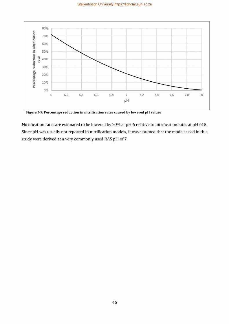
46

Figure 3-5: Percentage reduction in nitrification rates caused by lowered pH values

Nitrification rates are estimated to be lowered by 70% at pH 6 relative to nitrification rates at pH of 8.

Since pH was usually not reported in nitrification models, it was assumed that the models used in this

study were derived at a very commonly used RAS pH of 7.


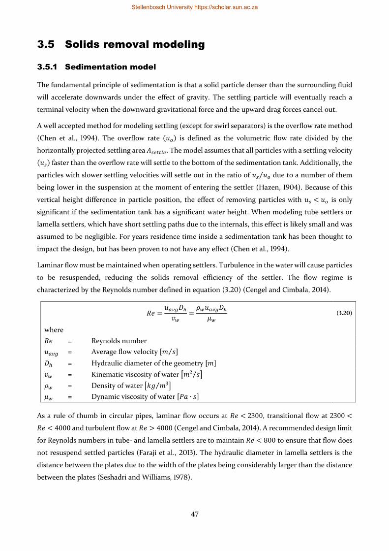
47

3.5 Solids removal modeling

3.5.1 Sedimentation model

The fundamental principle of sedimentation is that a solid particle denser than the surrounding fluid

will accelerate downwards under the effect of gravity. The settling particle will eventually reach a

terminal velocity when the downward gravitational force and the upward drag forces cancel out.

A well accepted method for modeling settling (except for swirl separators) is the overflow rate method

(Chen et al., 1994). The overflow rate (𝑢𝑜) is defined as the volumetric flow rate divided by the

horizontally projected settling area 𝐴𝑠𝑒𝑡𝑡𝑙𝑒. The model assumes that all particles with a settling velocity

(𝑢𝑠) faster than the overflow rate will settle to the bottom of the sedimentation tank. Additionally, the

particles with slower settling velocities will settle out in the ratio of 𝑢𝑠 𝑢𝑜⁄ due to a number of them

being lower in the suspension at the moment of entering the settler (Hazen, 1904). Because of this

vertical height difference in particle position, the effect of removing particles with 𝑢𝑠 < 𝑢𝑜 is only

significant if the sedimentation tank has a significant water height. When modeling tube settlers or

lamella settlers, which have short settling paths due to the internals, this effect is likely small and was

assumed to be negligible. For years residence time inside a sedimentation tank has been thought to

impact the design, but has been proven to not have any effect (Chen et al., 1994).

Laminar flow must be maintained when operating settlers. Turbulence in the water will cause particles

to be resuspended, reducing the solids removal efficiency of the settler. The flow regime is

characterized by the Reynolds number defined in equation (3.20) (Cengel and Cimbala, 2014).

𝑅𝑒 =𝑢𝑎𝑣𝑔𝐷ℎ

𝑣𝑤=

𝜌𝑤𝑢𝑎𝑣𝑔𝐷ℎ

𝜇𝑤 (3.20)

where

𝑅𝑒 = Reynolds number

𝑢𝑎𝑣𝑔 = Average flow velocity [𝑚 𝑠⁄ ]

𝐷ℎ = Hydraulic diameter of the geometry [𝑚]

𝑣𝑤 = Kinematic viscosity of water [𝑚2 𝑠⁄ ]

𝜌𝑤 = Density of water [𝑘𝑔 𝑚3⁄ ]

𝜇𝑤 = Dynamic viscosity of water [𝑃𝑎 ∙ 𝑠]

As a rule of thumb in circular pipes, laminar flow occurs at 𝑅𝑒 < 2300, transitional flow at 2300 <

𝑅𝑒 < 4000 and turbulent flow at 𝑅𝑒 > 4000 (Cengel and Cimbala, 2014). A recommended design limit

for Reynolds numbers in tube- and lamella settlers are to maintain 𝑅𝑒 < 800 to ensure that flow does

not resuspend settled particles (Faraji et al., 2013). The hydraulic diameter in lamella settlers is the

distance between the plates due to the width of the plates being considerably larger than the distance

between the plates (Seshadri and Williams, 1978).


48

In order to estimate the efficiency of a designed settler, the settling rate of the suspension needs to be

determined. The simplest method to predict the settling rate of a particle is by Stokes’ Law (Stokes,

1851). Stokes’ Law only applies to particles with a very low particle Reynolds Number (< 1), which is

the case for suspended solids produced in aquaculture systems. Stokes’ Law is given by equation (3.21).

𝑢𝑠 =𝑔(𝜌𝑝 − 𝜌𝑤)𝐷𝑝

2

18𝜇𝑤 (3.21)

where

𝑢𝑠 = Settling velocity [𝑚 𝑠⁄ ]

𝑔 = Gravitational acceleration [𝑚 𝑠2⁄ ]

𝜌𝑝 = Particle density [𝑘𝑔 𝑚3⁄ ]

𝐷𝑝 = Particle diameter [𝑚]

The specific gravity is used to represent the particle density. Chen et al. (1993) studied two RAS and

determined that the average SG of the suspended solids was 1.19, equaling an average particle density

of 1190 kg/m3.

Knowledge of the particle size distribution of the suspension is required to calculate the settling rates

for the entire suspension. Various studies have investigated the particle size distributions. Chen et al.

(1993) found that more than half of the number of particles were smaller than 10 µm, but particles

larger than 200 µm were excluded by pre-filtering. They also found that 50% of the particle mass is

contained in particles smaller than 20 µm. Fernandes et al. (2014) found that 50% of the particle mass

is contained in particles smaller than 60 µm, however it should be noted that pre-filtering was not

done in this study. The larger mass contained in the smaller particles could be due to breakages of

particles by pumping. It should also be noted that the particle size distribution can vary greatly from

system to system depending on the fish species, feed formulation and system configuration. No

particle size distribution data from a RAS similar to the RAS of focus in this study was found, and

therefore, due to the inability to obtain the required data an alternative method other than Stoke’s

Law had to be found for determining expected settling rates.

3.5.2 Solids settling characterization experiment

In order to determine settling rates to design a suitable solid settling unit, an experimental approach

was followed to measure the settling rates of the solids likely to be encountered in the designed RAS.

3.5.2.1 Methodology

Wong and Piedrahita (2000) proposed an experimental methodology for characterizing settling rates

of a RAS solids suspension. Using their methodology, the mass distribution of particles with different

settling rates can be experimentally determined for a specific RAS solids sample. A specific species had

to be chosen to be characterized for the design. It was decided to measure data for African catfish

solids due to observations at Welgevallen of African catfish feces breaking more readily into finer

solids than tilapia, meaning that African catfish solids are likely to have slower settling rates than


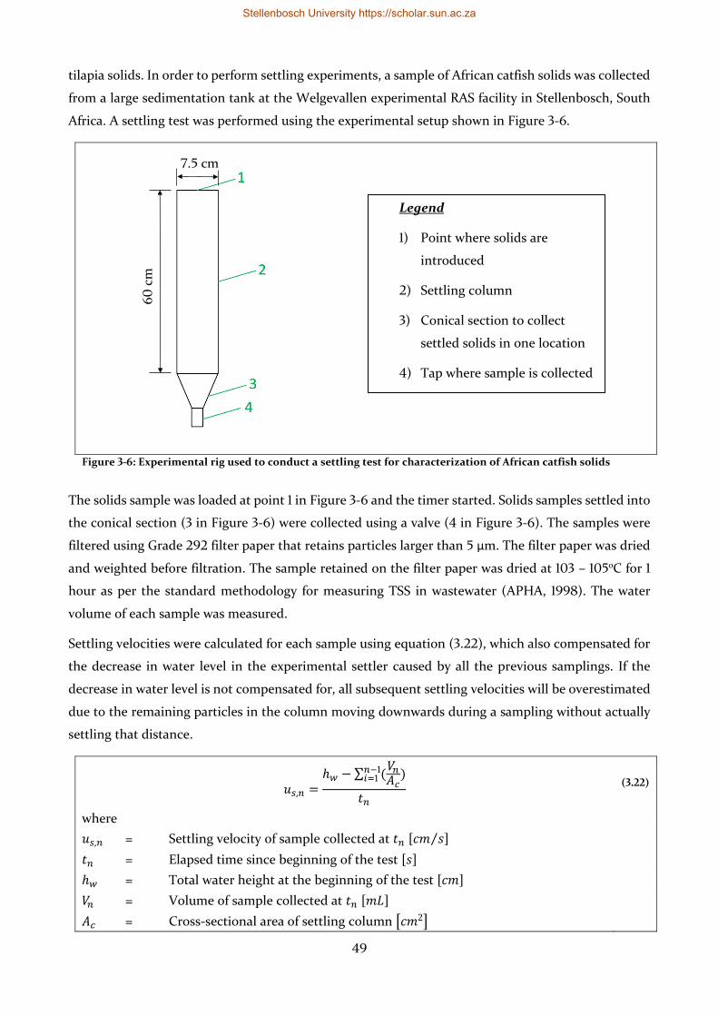
49

tilapia solids. In order to perform settling experiments, a sample of African catfish solids was collected

from a large sedimentation tank at the Welgevallen experimental RAS facility in Stellenbosch, South

Africa. A settling test was performed using the experimental setup shown in Figure 3-6.

Figure 3-6: Experimental rig used to conduct a settling test for characterization of African catfish solids

The solids sample was loaded at point 1 in Figure 3-6 and the timer started. Solids samples settled into

the conical section (3 in Figure 3-6) were collected using a valve (4 in Figure 3-6). The samples were

filtered using Grade 292 filter paper that retains particles larger than 5 μm. The filter paper was dried

and weighted before filtration. The sample retained on the filter paper was dried at 103 – 105oC for 1

hour as per the standard methodology for measuring TSS in wastewater (APHA, 1998). The water

volume of each sample was measured.

Settling velocities were calculated for each sample using equation (3.22), which also compensated for

the decrease in water level in the experimental settler caused by all the previous samplings. If the

decrease in water level is not compensated for, all subsequent settling velocities will be overestimated

due to the remaining particles in the column moving downwards during a sampling without actually

settling that distance.

𝑢𝑠,𝑛 =ℎ𝑤 − ∑ (

𝑉𝑛𝐴𝑐

𝑛−1𝑖=1 )

𝑡𝑛

(3.22)

where

𝑢𝑠,𝑛 = Settling velocity of sample collected at 𝑡𝑛 [𝑐𝑚 𝑠⁄ ]

𝑡𝑛 = Elapsed time since beginning of the test [𝑠]

ℎ𝑤 = Total water height at the beginning of the test [𝑐𝑚]

𝑉𝑛 = Volume of sample collected at 𝑡𝑛 [𝑚𝐿]

𝐴𝑐 = Cross-sectional area of settling column [𝑐𝑚2]

Legend

1) Point where solids are

introduced

2) Settling column

3) Conical section to collect

settled solids in one location

4) Tap where sample is collected

60

cm

7.5 cm


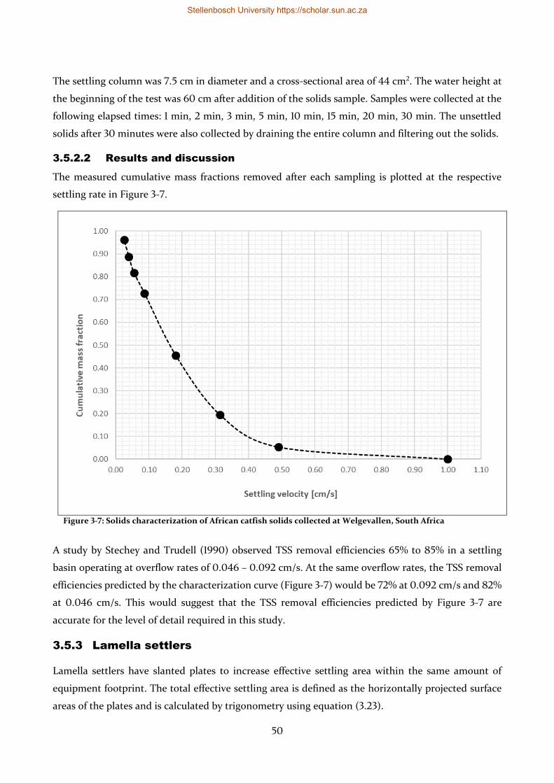
50

The settling column was 7.5 cm in diameter and a cross-sectional area of 44 cm2. The water height at

the beginning of the test was 60 cm after addition of the solids sample. Samples were collected at the

following elapsed times: 1 min, 2 min, 3 min, 5 min, 10 min, 15 min, 20 min, 30 min. The unsettled

solids after 30 minutes were also collected by draining the entire column and filtering out the solids.

3.5.2.2 Results and discussion

The measured cumulative mass fractions removed after each sampling is plotted at the respective

settling rate in Figure 3-7.

Figure 3-7: Solids characterization of African catfish solids collected at Welgevallen, South Africa

A study by Stechey and Trudell (1990) observed TSS removal efficiencies 65% to 85% in a settling

basin operating at overflow rates of 0.046 – 0.092 cm/s. At the same overflow rates, the TSS removal

efficiencies predicted by the characterization curve (Figure 3-7) would be 72% at 0.092 cm/s and 82%

at 0.046 cm/s. This would suggest that the TSS removal efficiencies predicted by Figure 3-7 are

accurate for the level of detail required in this study.

3.5.3 Lamella settlers

Lamella settlers have slanted plates to increase effective settling area within the same amount of

equipment footprint. The total effective settling area is defined as the horizontally projected surface

areas of the plates and is calculated by trigonometry using equation (3.23).


51

𝐴𝑠𝑒𝑡𝑡𝑙𝑒 = 𝑛𝑝𝑙𝑎𝑡𝑒 ∙ 𝐿𝑝𝑙𝑎𝑡𝑒 𝑙𝑒𝑛𝑔𝑡ℎ ∙ 𝐿𝑝𝑙𝑎𝑡𝑒 𝑤𝑖𝑑𝑡ℎ ∙ cos Φ (3.23)

where

𝑛𝑝𝑙𝑎𝑡𝑒 = Number of plates

𝐴𝑠𝑒𝑡𝑡𝑙𝑒 = Horizontally projected settling area [𝑚2]

𝐿𝑝𝑙𝑎𝑡𝑒 𝑙𝑒𝑛𝑔𝑡ℎ = Lamella settler plate length [𝑚]

𝐿𝑝𝑙𝑎𝑡𝑒 𝑤𝑖𝑑𝑡ℎ = Lamella settler plate width [𝑚]

Φ = Lamella settler plate inclination with the horizontal plane [𝑑𝑒𝑔𝑟𝑒𝑒𝑠]

3.5.4 Sand filter model

Sand filters have a typical TSS removal efficiency of 95%. As a rule of thumb, 95% of particles larger

than 6 μm and 15 μm are removed when using 0.3 mm and 0.5 mm sand grains respectively (Lekang,

2007). Pressure drop over a sand filter will increase as the solids are entrapped. The minimum and

maximum pressure drop experienced in a sand filter was obtained from manufacturers and not

modeled.


52

3.6 Aeration and degassing models

3.6.1 Aeration modeling

Aeration by submerged air diffusers, also known as airstones, was modeled in this study due to (1)

general use in experimental RAS and (2) widespread availability and low cost of the technology.

Fundamentally the diffusion mass transfer of oxygen to and from water can be modeled using equation

(3.24) (Wik et al., 2009).

𝑚𝑂2= 𝑉 ∙ 𝐾𝐿𝑎𝑂2

∙ (𝐶𝑂2

𝑠𝑎𝑡 − 𝐶𝑂2) (3.24)

where

𝑚𝑂2 = Mass transfer rate of oxygen into the water [𝑔 𝑑𝑎𝑦⁄ ]

𝑉 = Volume of the vessel [𝑚3]

𝐾𝐿𝑎𝑂2 = Overall oxygen mass transfer coefficient [1 𝑑𝑎𝑦⁄ ]

𝐶𝑂2

𝑠𝑎𝑡 = Saturation concentration of oxygen in water [𝑚𝑔/𝐿]

𝐶𝑂2 = Dissolved oxygen concentration [𝑚𝑔/𝐿]

The saturation concentration of oxygen in clean water can be estimated using equation (3.25)

(Timmons and Ebeling, 2007).

(𝐶𝑂2


=1 003 200

(95

∙ 𝑇 + 32)0.625

∙ (760 +𝜁

107.6)

(3.25)

where

(𝐶𝑂2


= Oxygen saturation concentration under clean conditions [𝑚𝑔 𝐿⁄ ]

𝑇 = Water temperature [℃]

𝜁 = Altitude of the site [𝑚]

𝐶𝑂2

𝑠𝑎𝑡 at field conditions can differ from 𝐶𝑂2

𝑠𝑎𝑡 in clean water due to TDS and TSS (Stenstrom and

Gilbert, 1981). This is quantified by the beta factor (𝛽) as in equation (3.26). A beta factor of 1.0 was

observed in catfish ponds (Shelton and Boyd, 1983).

𝛽 =(𝐶𝑂2


(𝐶𝑂2


(3.26)

where

(𝐶𝑂2


= Oxygen saturation concentration under field conditions [𝑚𝑔 𝐿⁄ ]

The ratio of the oxygen transfer coefficients at field and clean water conditions is represented by the

alpha factor (𝛼) as in equation (3.27). An alpha factor of 1.00 has been observed in catfish ponds

(Shelton and Boyd, 1983).


53

𝛼 =(𝐾𝐿𝑎𝑂2

)𝐹𝑊

(𝐾𝐿𝑎𝑂2)

𝐶𝑊

(3.27)

where

(𝐾𝐿𝑎𝑂2)

𝐹𝑊 = Overall oxygen mass transfer coefficient under field conditions

[1 𝑑𝑎𝑦⁄ ]

(𝐾𝐿𝑎𝑂2)

𝐶𝑊 = Overall oxygen mass transfer coefficient under clean water

conditions [1 𝑑𝑎𝑦⁄ ]

For provision of aeration to RAS, regenerative blowers are generally employed. The approximate

blower power consumption (𝑃𝑏𝑙𝑜𝑤𝑒𝑟) can be estimated using the transfer efficiency of the submerged

diffusers. This is used for optimization of aeration processes and was used in the optimization of the

oxygen concentration in the MBBRs (see section 4.5.4.1). The approximate blower power is estimated

using equations (3.28), (3.29) and (3.30) (Colt and Tchobanoglous, 1981; Huguenin and Colt, 2002).

𝑃𝑏𝑙𝑜𝑤𝑒𝑟 =𝑚𝑂2

𝑁𝐹𝑊 ∙ 𝜂𝑏𝑙𝑜𝑤𝑒𝑟 (3.28)

𝑁𝐹𝑊 =𝑁𝑠𝑡𝑑 ∙ (𝛽(𝐶𝑂2


− 𝐶𝑂2) ∙ 1.024𝑇−20 ∙ 𝛼

(𝐶𝑂2


(3.29)

(𝐶𝑂2


= (𝐶𝑂2


∙ (1.00 + 𝜑ℎ𝑑𝑖𝑓𝑓𝑢𝑠𝑒𝑟) (3.30)

where

𝑃𝑏𝑙𝑜𝑤𝑒𝑟 = Blower input power [ℎ𝑝]

𝑁𝐹𝑊 = Oxygen transfer efficiency at field conditions [𝑘𝑔 𝑂2 (𝑘𝑊 ∙ ℎ)⁄ ]

𝜂𝑏𝑙𝑜𝑤𝑒𝑟 = Blower efficiency

𝑚𝑂2 = Mass transfer rate of oxygen into the water [𝑘𝑔 𝑂2 ℎ⁄ ]

𝑁𝑠𝑡𝑑 = Oxygen transfer efficiency at standard conditions [𝑘𝑔 𝑂2 (𝑘𝑊 ∙ ℎ)⁄ ]

(𝐶𝑂2


= Mean effective dissolved oxygen saturation concentration [𝑚𝑔 𝐿⁄ ]

𝑇 = Temperature [℃]

𝜑 = 0.008 for coarse bubble diffusers, 0.016 for fine bubble diffusers

ℎ𝑑𝑖𝑓𝑓𝑢𝑠𝑒𝑟 = Diffuser depth [𝑚]

Regenerative blowers typically have an efficiency of 66% (CFW Fans, 2019a; Huguenin and Colt,

2002). For the purposes of conceptual design, standard oxygen transfer efficiencies of

0.6 𝑘𝑔 𝑂2 (𝑘𝑊 ∙ ℎ)⁄ and 1.2 𝑘𝑔 𝑂2 (𝑘𝑊 ∙ ℎ)⁄ can be used for coarse and fine bubble diffusers

respectively (Huguenin and Colt, 2002).

Predicting the oxygen mass transfer rate using equation (3.24) requires modeling 𝐾𝐿𝑎𝑂2. The overall

oxygen mass transfer coefficient, 𝐾𝐿𝑎𝑂2, is determined by gas bubble size, water turbulence, system

geometry, water depth, temperature, air flow rate, air flow rate per diffuser and tank water surface


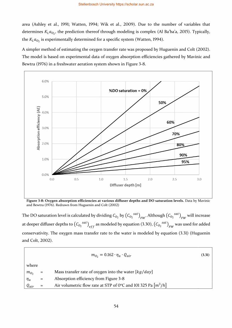
54

area (Ashley et al., 1991; Watten, 1994; Wik et al., 2009). Due to the number of variables that

determines 𝐾𝐿𝑎𝑂2, the prediction thereof through modeling is complex (Al Ba’ba’a, 2015). Typically,

the 𝐾𝐿𝑎𝑂2 is experimentally determined for a specific system (Watten, 1994).

A simpler method of estimating the oxygen transfer rate was proposed by Huguenin and Colt (2002).

The model is based on experimental data of oxygen absorption efficiencies gathered by Mavinic and

Bewtra (1976) in a freshwater aeration system shown in Figure 3-8.

Figure 3-8: Oxygen absorption efficiencies at various diffuser depths and DO saturation levels. Data by Mavinic and Bewtra (1976). Redrawn from Huguenin and Colt (2002)

The DO saturation level is calculated by dividing 𝐶𝑂2 by (𝐶𝑂2


. Although (𝐶𝑂2


will increase

at deeper diffuser depths to (𝐶𝑂2


as modeled by equation (3.30), (𝐶𝑂2


was used for added

conservativity. The oxygen mass transfer rate to the water is modeled by equation (3.31) (Huguenin

and Colt, 2002).

𝑚𝑂2= 0.162 ∙ 𝜂𝑎 ∙ 𝑄𝑎𝑖𝑟 (3.31)

where

𝑚𝑂2 = Mass transfer rate of oxygen into the water [𝑘𝑔 𝑑𝑎𝑦⁄ ]

𝜂𝑎 = Absorption efficiency from Figure 3-8

𝑄𝑎𝑖𝑟 = Air volumetric flow rate at STP of 0oC and 101 325 Pa [𝑚3/ℎ]


55

3.6.2 Gas supersaturation

Total dissolved gas pressure (TGP) is determined by the summing the gas tensions (also known as

partial pressure) of the dissolved gases as in equation (3.33) after calculating each individual gas

tension using equation (3.32). Carbon dioxide was not included due to its low concentration observed

in this study making its contribution to TGP negligible.

𝜏𝑖 = 𝐹𝑖𝐶𝑖 (3.32)

𝑇𝐺𝑃 = ∑ 𝜏𝑖 (3.33)

where

𝜏𝑖 = Gas tension of component 𝑖 [𝑚𝑚𝐻𝑔]

𝐹𝑖 = Gas tension factor of component 𝑖 [𝑚𝑚𝐻𝑔 (𝑚𝑔 𝐿⁄ )⁄ ]

𝐶𝑖 = Concentration of component 𝑖 [𝑚𝑔/𝐿]

𝑇𝐺𝑃 = Total dissolved gas pressure [𝑚𝑚𝐻𝑔]

The gas tension factors and solubilities of oxygen and nitrogen are given in APPENDIX F.

3.6.3 Carbon dioxide degassing model

Carbon dioxide degassing due to aeration was modeled according to the method by Wik et al. (2009)

using equation (3.34).

𝑚𝐶𝑂2= 𝑉 ∙ 𝐾𝐿𝑎𝐶𝑂2

∙ (𝐶𝐶𝑂2

𝑠𝑎𝑡 − 𝐶𝐶𝑂2) (3.34)

where

𝑚𝐶𝑂2 = Mass transfer rate of carbon dioxide into the water [𝑔 𝑑𝑎𝑦⁄ ]

𝑉 = Volume of the vessel [𝑚3]

𝐾𝐿𝑎𝐶𝑂2 = Overall carbon dioxide mass transfer coefficient [1 𝑑𝑎𝑦⁄ ]

𝐶𝐶𝑂2

𝑠𝑎𝑡 = Saturation concentration of carbon dioxide in water [𝑚𝑔/𝐿]

𝐶𝐶𝑂2 = Dissolved carbon dioxide concentration [𝑚𝑔/𝐿]

𝐶𝐶𝑂2

𝑠𝑎𝑡 is equal to 0.5 mg/L due to it being the concentration of CO2 in ambient air (Timmons and

Ebeling, 2007, p. 107). 𝐾𝐿𝑎𝐶𝑂2 can be estimated using a ratio of

𝐾𝐿𝑎𝐶𝑂2

𝐾𝐿𝑎𝑂2

= 0.9, and 𝐾𝐿𝑎𝑂2 can be

estimated by rearranging equation (3.24) to yield equation (3.35).

𝐾𝐿𝑎𝑂2=

𝑚𝑂2

𝑉 ∙ (𝐶𝑂2

𝑠𝑎𝑡 − 𝐶𝑂2) (3.35)

Comprehensive models for CO2 degassers are available (Grace and Piedrahita, 1994; Vinci et al., 1996).

However, within the design parameters of the current study, a dedicated CO2 degassing unit was not

required as enough CO2 was removed by aeration in the fish tanks and biofilters (see section 4.6.5).


56

3.7 Pipe flow pressure drop

Pressure drop in pipes is determined by the flow velocity, pipe diameter, surface roughness of the pipe,

pipe length, fluid properties and flow regime (Cengel and Cimbala, 2014). Pressure drop is also

expressed in terms of equivalent water body height known as head loss. Head loss is calculated using

equation (3.36).

ℎ𝐿 =𝑓 ∙ 𝐿𝑝𝑖𝑝𝑒 ∙ 𝑢𝑎𝑣𝑔

2

2𝑔 ∙ 𝐷𝑝𝑖𝑝𝑒 (3.36)

where

ℎ𝐿 = Head loss [𝑚]

𝑓 = Darcy friction factor

𝐿𝑝𝑖𝑝𝑒 = Pipe length [𝑚]

𝑢𝑎𝑣𝑔 = Average flow velocity [𝑚 𝑠⁄ ]


𝐷𝑝𝑖𝑝𝑒 = Pipe diameter [𝑚]

The effect of wall friction is accounted for using the Darcy friction factor (𝑓). The following methods

were used to calculate the friction factor.

Laminar flow through circular pipe: 𝑓 =64.00

𝑅𝑒 (3.37)

Turbulent flow through circular pipe: 𝑓 = (1

−1.8 log(6.9

𝑅𝑒+(

𝜉 𝐷𝑝𝑖𝑝𝑒⁄

3.7)

1.11

)

)

2

(3.38)

Laminar flow between parallel plates: 𝑓 =96.00

𝑅𝑒 (3.39)

where

𝑅𝑒 = Reynolds number (see section 3.5.1)

𝜉 = Pipe surface roughness [𝑚]

Minor head losses are introduced by components such as valves and heat exchangers and changes in

flow geometry such as bends and pipe diameter expansion or contraction. Except for heat exchangers,

the minor head losses were assumed to be negligible due to the early stage of design and lack of minor

losses that can be expected in the system.

Hydraulic head is the head loss introduced when pumping from a water surface with a lower elevation

than the destination, and the value is equal to the height difference between the two points. When

gravity flow occurs, the difference in water level of the two free water surfaces will be equal to the total

head loss within the piping system where the gravity flow occurs.


57

3.8 Fish tank mass balances

A mass balance over a RAS system volume is expressed as 𝑚𝑎𝑠𝑠 𝑎𝑐𝑐𝑢𝑚𝑢𝑙𝑎𝑡𝑖𝑜𝑛 = 𝑚𝑎𝑠𝑠 𝑖𝑛 − 𝑚𝑎𝑠𝑠 𝑜𝑢𝑡.

Mass balances were needed in this design to size the recirculation pumps to allow enough circulation

to avoid accumulation of waste products in the fish tanks. Thus, the chosen system volume was the

fish tanks. Due to the low make-up flow rates in RAS culture (99% of water is recycled), the effect of

waste removal by effluent water was assumed to be negligible and omitted from the mass balance

calculations.

The general mass balance of a material over the fish tanks is expressed as:

(𝑚𝑎𝑐𝑐)𝑖 = (𝑚𝑟𝑒𝑐𝑖𝑟𝑐,𝑖𝑛)𝑖

+ (𝑚𝑝𝑟𝑜𝑑)𝑖

− (𝑚𝑟𝑒𝑐𝑖𝑟𝑐,𝑜𝑢𝑡)𝑖

− (𝑚𝑐𝑜𝑛𝑠)𝑖 (3.40)

where

(𝑚𝑎𝑐𝑐)𝑖 = Mass accumulation rate of component 𝑖 [𝑔 𝑑𝑎𝑦⁄ ]

(𝑚𝑟𝑒𝑐𝑖𝑟𝑐,𝑖𝑛)𝑖 = Influent mass flow rate of component 𝑖 [𝑔 𝑑𝑎𝑦⁄ ]

(𝑚𝑝𝑟𝑜𝑑)𝑖 = Production rate of component 𝑖 [𝑔 𝑑𝑎𝑦⁄ ]

(𝑚𝑟𝑒𝑐𝑖𝑟𝑐,𝑜𝑢𝑡)𝑖 = Effluent mass flow rate of component 𝑖 [𝑔 𝑑𝑎𝑦⁄ ]

(𝑚𝑐𝑜𝑛𝑠)𝑖 = Consumption rate of component 𝑖 [𝑔 𝑑𝑎𝑦⁄ ]

Applying equation (3.40) to the major components of interest, namely oxygen, carbon dioxide, total

suspended solids and total ammonia nitrogen yields the following equations. It is assumed that the

mass accumulation rate of each component in the fish tanks is zero. The influent and effluent mass

flow rates are shown in terms of recirculating flow rate and component concentration.

𝑄𝑟𝑒𝑐𝑖𝑟𝑐 ∙ 𝐶𝑂2,𝑖𝑛 + (𝑚𝑝𝑟𝑜𝑑)𝑂2

− 𝑄𝑟𝑒𝑐𝑖𝑟𝑐 ∙ 𝐶𝑂2,𝑜𝑢𝑡 − (𝑚𝑐𝑜𝑛𝑠)𝑂2= 0 (3.41)

𝑄𝑟𝑒𝑐𝑖𝑟𝑐 ∙ 𝐶𝐶𝑂2,𝑖𝑛 + (𝑚𝑝𝑟𝑜𝑑)𝐶𝑂2

− 𝑄𝑟𝑒𝑐𝑖𝑟𝑐 ∙ 𝐶𝐶𝑂2,𝑜𝑢𝑡 − (𝑚𝑐𝑜𝑛𝑠)𝐶𝑂2= 0 (3.42)

𝑄𝑟𝑒𝑐𝑖𝑟𝑐 ∙ 𝐶𝑇𝑆𝑆,𝑖𝑛 + (𝑚𝑝𝑟𝑜𝑑)𝑇𝑆𝑆

− 𝑄𝑟𝑒𝑐𝑖𝑟𝑐 ∙ 𝐶𝑇𝑆𝑆,𝑜𝑢𝑡 = 0 (3.43)

𝑄𝑟𝑒𝑐𝑖𝑟𝑐 ∙ 𝐶𝑇𝐴𝑁,𝑖𝑛 + (𝑚𝑝𝑟𝑜𝑑)𝑇𝐴𝑁

− 𝑄𝑟𝑒𝑐𝑖𝑟𝑐 ∙ 𝐶𝑇𝐴𝑁,𝑜𝑢𝑡 = 0 (3.44)

where

𝑄𝑟𝑒𝑐𝑖𝑟𝑐 = Recirculation flow rate [𝑚3 𝑑𝑎𝑦⁄ ]

𝐶𝑖,𝑖𝑛 = Concentration of influent component 𝑖 [𝑚𝑔 𝐿⁄ ]

𝐶𝑖,𝑜𝑢𝑡 = Concentration of effluent component 𝑖 [𝑚𝑔 𝐿⁄ ]

(𝑚𝑝𝑟𝑜𝑑)𝑂2

= Oxygen added by aeration [𝑔 𝑑𝑎𝑦⁄ ]

(𝑚𝑐𝑜𝑛𝑠)𝑂2 = Oxygen consumed by fish metabolism [𝑔 𝑑𝑎𝑦⁄ ]

(𝑚𝑝𝑟𝑜𝑑)𝐶𝑂2

= Carbon dioxide excreted by fish [𝑔 𝑑𝑎𝑦⁄ ]

(𝑚𝑐𝑜𝑛𝑠)𝐶𝑂2 = Carbon dioxide removed by aeration [𝑔 𝑑𝑎𝑦⁄ ]

(𝑚𝑝𝑟𝑜𝑑)𝑇𝑆𝑆

= Total suspended solids produced by feeding [𝑔 𝑑𝑎𝑦⁄ ]


= Total ammonia nitrogen produced by feeding [𝑔 𝑑𝑎𝑦⁄ ]


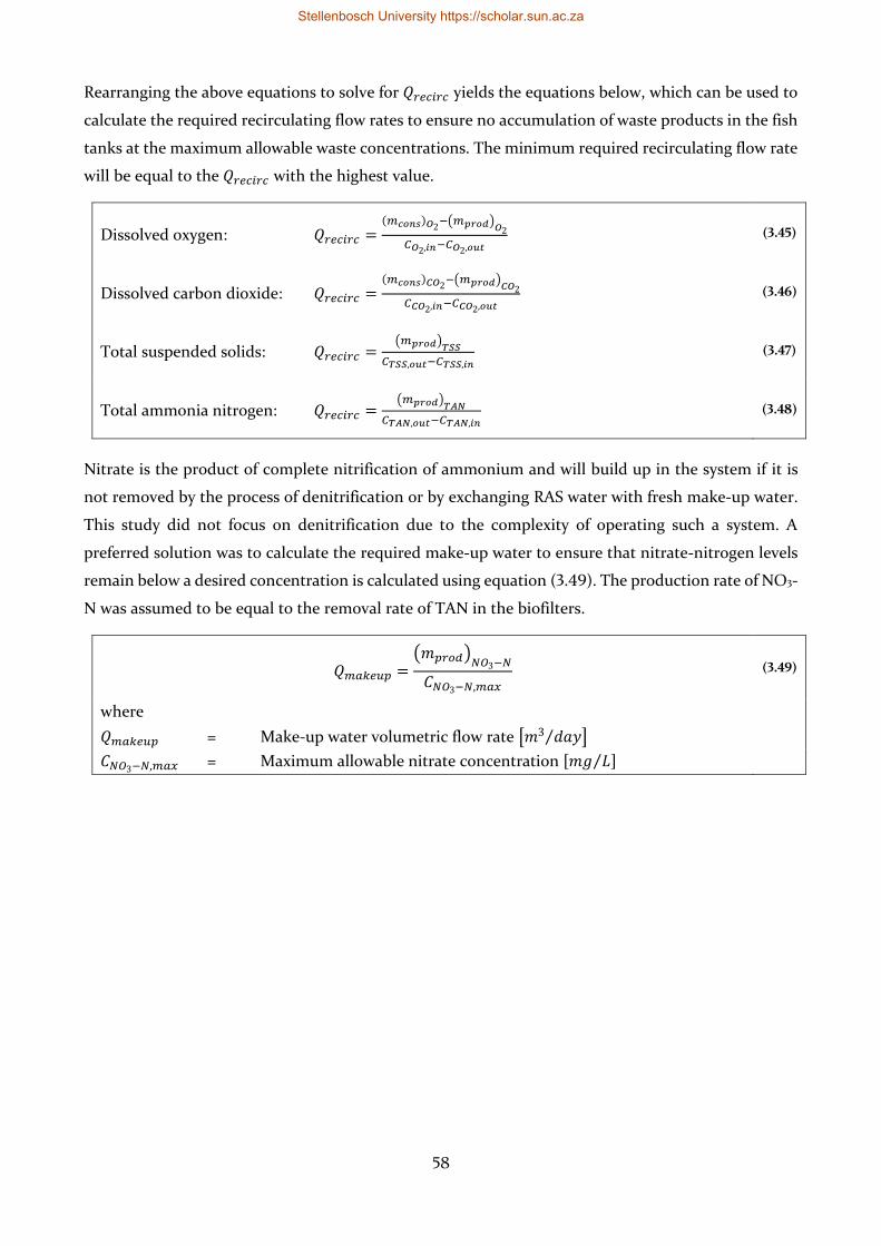
58

Rearranging the above equations to solve for 𝑄𝑟𝑒𝑐𝑖𝑟𝑐 yields the equations below, which can be used to

calculate the required recirculating flow rates to ensure no accumulation of waste products in the fish

tanks at the maximum allowable waste concentrations. The minimum required recirculating flow rate

will be equal to the 𝑄𝑟𝑒𝑐𝑖𝑟𝑐 with the highest value.

Dissolved oxygen: 𝑄𝑟𝑒𝑐𝑖𝑟𝑐 =(𝑚𝑐𝑜𝑛𝑠)𝑂2

−(𝑚𝑝𝑟𝑜𝑑)𝑂2

𝐶𝑂2,𝑖𝑛−𝐶𝑂2,𝑜𝑢𝑡 (3.45)

Dissolved carbon dioxide: 𝑄𝑟𝑒𝑐𝑖𝑟𝑐 =(𝑚𝑐𝑜𝑛𝑠)𝐶𝑂2

−(𝑚𝑝𝑟𝑜𝑑)𝐶𝑂2

𝐶𝐶𝑂2,𝑖𝑛−𝐶𝐶𝑂2,𝑜𝑢𝑡 (3.46)

Total suspended solids: 𝑄𝑟𝑒𝑐𝑖𝑟𝑐 =(𝑚𝑝𝑟𝑜𝑑)

𝑇𝑆𝑆

𝐶𝑇𝑆𝑆,𝑜𝑢𝑡−𝐶𝑇𝑆𝑆,𝑖𝑛 (3.47)

Total ammonia nitrogen: 𝑄𝑟𝑒𝑐𝑖𝑟𝑐 =(𝑚𝑝𝑟𝑜𝑑)

𝑇𝐴𝑁

𝐶𝑇𝐴𝑁,𝑜𝑢𝑡−𝐶𝑇𝐴𝑁,𝑖𝑛 (3.48)

Nitrate is the product of complete nitrification of ammonium and will build up in the system if it is

not removed by the process of denitrification or by exchanging RAS water with fresh make-up water.

This study did not focus on denitrification due to the complexity of operating such a system. A

preferred solution was to calculate the required make-up water to ensure that nitrate-nitrogen levels

remain below a desired concentration is calculated using equation (3.49). The production rate of NO3-

N was assumed to be equal to the removal rate of TAN in the biofilters.

𝑄𝑚𝑎𝑘𝑒𝑢𝑝 =(𝑚𝑝𝑟𝑜𝑑)

𝑁𝑂3−𝑁

𝐶𝑁𝑂3−𝑁,𝑚𝑎𝑥 (3.49)

where

𝑄𝑚𝑎𝑘𝑒𝑢𝑝 = Make-up water volumetric flow rate [𝑚3 𝑑𝑎𝑦⁄ ]

𝐶𝑁𝑂3−𝑁,𝑚𝑎𝑥 = Maximum allowable nitrate concentration [𝑚𝑔 𝐿⁄ ]


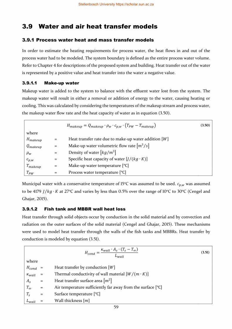
59

3.9 Water and air heat transfer models

3.9.1 Process water heat and mass transfer models

In order to estimate the heating requirements for process water, the heat flows in and out of the

process water had to be modeled. The system boundary is defined as the entire process water volume.

Refer to Chapter 4 for descriptions of the proposed system and building. Heat transfer out of the water

is represented by a positive value and heat transfer into the water a negative value.

3.9.1.1 Make-up water

Makeup water is added to the system to balance with the effluent water lost from the system. The

makeup water will result in either a removal or addition of energy to the water, causing heating or

cooling. This was calculated by considering the temperatures of the makeup stream and process water,

the makeup water flow rate and the heat capacity of water as in equation (3.50).

𝐻𝑚𝑎𝑘𝑒𝑢𝑝 = 𝑄𝑚𝑎𝑘𝑒𝑢𝑝 ∙ 𝜌𝑤 ∙ 𝑐𝑝,𝑤 ∙ (𝑇𝑃𝑊 − 𝑇𝑚𝑎𝑘𝑒𝑢𝑝) (3.50)

where

𝐻𝑚𝑎𝑘𝑒𝑢𝑝 = Heat transfer rate due to make-up water addition [𝑊]

𝑄𝑚𝑎𝑘𝑒𝑢𝑝 = Make-up water volumetric flow rate [𝑚3 𝑠⁄ ]

𝜌𝑤 = Density of water [𝑘𝑔 𝑚3⁄ ]

𝑐𝑝,𝑤 = Specific heat capacity of water [𝐽 (𝑘𝑔 ∙ 𝐾)⁄ ]

𝑇𝑚𝑎𝑘𝑒𝑢𝑝 = Make-up water temperature [℃]

𝑇𝑃𝑊 = Process water temperature [℃]

Municipal water with a conservative temperature of 15oC was assumed to be used. 𝑐𝑝,𝑤 was assumed

to be 4179 𝐽 𝑘𝑔 ∙ 𝐾⁄ at 27oC and varies by less than 0.5% over the range of 10oC to 30oC (Cengel and

Ghajar, 2015).

3.9.1.2 Fish tank and MBBR wall heat loss

Heat transfer through solid objects occur by conduction in the solid material and by convection and

radiation on the outer surfaces of the solid material (Cengel and Ghajar, 2015). These mechanisms

were used to model heat transfer through the walls of the fish tanks and MBBRs. Heat transfer by

conduction is modeled by equation (3.51).

𝐻𝑐𝑜𝑛𝑑 =𝜅𝑤𝑎𝑙𝑙 ∙ 𝐴𝑠 ∙ (𝑇𝑠 − 𝑇∞)

𝐿𝑤𝑎𝑙𝑙 (3.51)

where

𝐻𝑐𝑜𝑛𝑑 = Heat transfer by conduction [𝑊]

𝜅𝑤𝑎𝑙𝑙 = Thermal conductivity of wall material [𝑊 (𝑚 ∙ 𝐾)⁄ ]

𝐴𝑠 = Heat transfer surface area [𝑚2]

𝑇∞ = Air temperature sufficiently far away from the surface [℃]

𝑇𝑠 = Surface temperature [℃]

𝐿𝑤𝑎𝑙𝑙 = Wall thickness [𝑚]


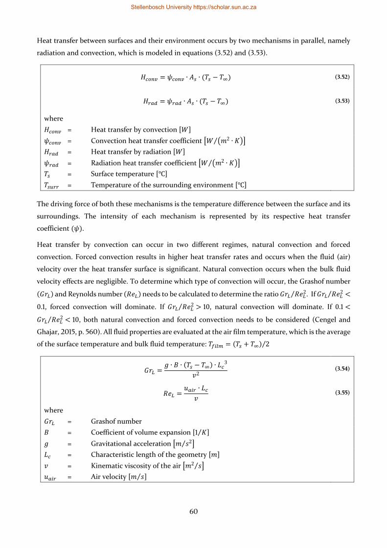
60

Heat transfer between surfaces and their environment occurs by two mechanisms in parallel, namely

radiation and convection, which is modeled in equations (3.52) and (3.53).

𝐻𝑐𝑜𝑛𝑣 = 𝜓𝑐𝑜𝑛𝑣 ∙ 𝐴𝑠 ∙ (𝑇𝑠 − 𝑇∞) (3.52)

𝐻𝑟𝑎𝑑 = 𝜓𝑟𝑎𝑑 ∙ 𝐴𝑠 ∙ (𝑇𝑠 − 𝑇∞) (3.53)

where

𝐻𝑐𝑜𝑛𝑣 = Heat transfer by convection [𝑊]

𝜓𝑐𝑜𝑛𝑣 = Convection heat transfer coefficient [𝑊 (𝑚2 ∙ 𝐾)⁄ ]

𝐻𝑟𝑎𝑑 = Heat transfer by radiation [𝑊]

𝜓𝑟𝑎𝑑 = Radiation heat transfer coefficient [𝑊 (𝑚2 ∙ 𝐾)⁄ ]

𝑇𝑠 = Surface temperature [℃]

𝑇𝑠𝑢𝑟𝑟 = Temperature of the surrounding environment [℃]

The driving force of both these mechanisms is the temperature difference between the surface and its

surroundings. The intensity of each mechanism is represented by its respective heat transfer

coefficient (𝜓).

Heat transfer by convection can occur in two different regimes, natural convection and forced

convection. Forced convection results in higher heat transfer rates and occurs when the fluid (air)

velocity over the heat transfer surface is significant. Natural convection occurs when the bulk fluid

velocity effects are negligible. To determine which type of convection will occur, the Grashof number

(𝐺𝑟𝐿) and Reynolds number (𝑅𝑒𝐿) needs to be calculated to determine the ratio 𝐺𝑟𝐿 𝑅𝑒𝐿2⁄ . If 𝐺𝑟𝐿 𝑅𝑒𝐿

2⁄ <

0.1, forced convection will dominate. If 𝐺𝑟𝐿 𝑅𝑒𝐿2⁄ > 10, natural convection will dominate. If 0.1 <

𝐺𝑟𝐿 𝑅𝑒𝐿2⁄ < 10, both natural convection and forced convection needs to be considered (Cengel and

Ghajar, 2015, p. 560). All fluid properties are evaluated at the air film temperature, which is the average

of the surface temperature and bulk fluid temperature: 𝑇𝑓𝑖𝑙𝑚 = (𝑇𝑠 + 𝑇∞) 2⁄

𝐺𝑟𝐿 =𝑔 ∙ 𝐵 ∙ (𝑇𝑠 − 𝑇∞) ∙ 𝐿𝑐

3

𝑣2 (3.54)

𝑅𝑒𝐿 =𝑢𝑎𝑖𝑟 ∙ 𝐿𝑐

𝑣 (3.55)

where

𝐺𝑟𝐿 = Grashof number

𝐵 = Coefficient of volume expansion [1 𝐾⁄ ]


𝐿𝑐 = Characteristic length of the geometry [𝑚]

𝑣 = Kinematic viscosity of the air [𝑚2 𝑠⁄ ]

𝑢𝑎𝑖𝑟 = Air velocity [𝑚 𝑠⁄ ]


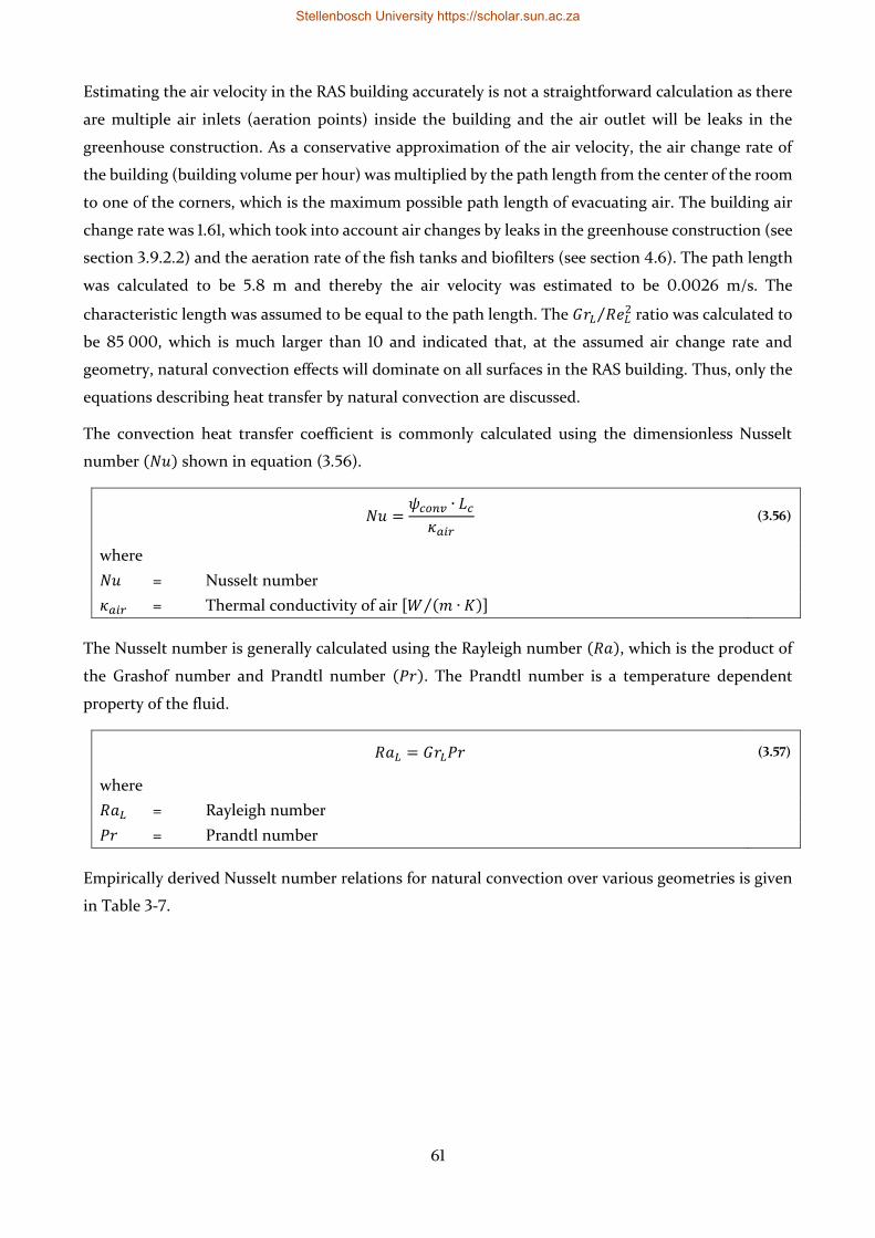
61

Estimating the air velocity in the RAS building accurately is not a straightforward calculation as there

are multiple air inlets (aeration points) inside the building and the air outlet will be leaks in the

greenhouse construction. As a conservative approximation of the air velocity, the air change rate of

the building (building volume per hour) was multiplied by the path length from the center of the room

to one of the corners, which is the maximum possible path length of evacuating air. The building air

change rate was 1.61, which took into account air changes by leaks in the greenhouse construction (see

section 3.9.2.2) and the aeration rate of the fish tanks and biofilters (see section 4.6). The path length

was calculated to be 5.8 m and thereby the air velocity was estimated to be 0.0026 m/s. The

characteristic length was assumed to be equal to the path length. The 𝐺𝑟𝐿 𝑅𝑒𝐿2⁄ ratio was calculated to

be 85 000, which is much larger than 10 and indicated that, at the assumed air change rate and

geometry, natural convection effects will dominate on all surfaces in the RAS building. Thus, only the

equations describing heat transfer by natural convection are discussed.

The convection heat transfer coefficient is commonly calculated using the dimensionless Nusselt

number (𝑁𝑢) shown in equation (3.56).

𝑁𝑢 =𝜓𝑐𝑜𝑛𝑣 ∙ 𝐿𝑐

𝜅𝑎𝑖𝑟 (3.56)

where

𝑁𝑢 = Nusselt number

𝜅𝑎𝑖𝑟 = Thermal conductivity of air [𝑊 (𝑚 ∙ 𝐾)⁄ ]

The Nusselt number is generally calculated using the Rayleigh number (𝑅𝑎), which is the product of

the Grashof number and Prandtl number (𝑃𝑟). The Prandtl number is a temperature dependent

property of the fluid.

𝑅𝑎𝐿 = 𝐺𝑟𝐿𝑃𝑟 (3.57)

where

𝑅𝑎𝐿 = Rayleigh number

𝑃𝑟 = Prandtl number

Empirically derived Nusselt number relations for natural convection over various geometries is given

in Table 3-7.


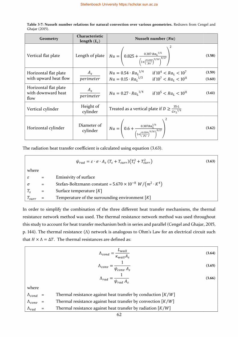
62

Table 3-7: Nusselt number relations for natural convection over various geometries. Redrawn from Cengel and Ghajar (2015).

Geometry Characteristic

length (𝑳𝒄) Nusselt number (𝑵𝒖)

Vertical flat plate Length of plate 𝑁𝑢 = (0.825 +0.387∙𝑅𝑎𝐿

1 6⁄

(1+(0.492

𝑃𝑟)

9 16⁄)

8 27⁄ )

2

(3.58)

Horizontal flat plate with upward heat flow

𝐴𝑠

𝑝𝑒𝑟𝑖𝑚𝑒𝑡𝑒𝑟

𝑁𝑢 = 0.54 ∙ 𝑅𝑎𝐿1 4⁄ if 104 < 𝑅𝑎𝐿 < 107

𝑁𝑢 = 0.15 ∙ 𝑅𝑎𝐿1 3⁄ if 107 < 𝑅𝑎𝐿 < 1011

(3.59)

(3.60)

Horizontal flat plate with downward heat flow

𝐴𝑠

𝑝𝑒𝑟𝑖𝑚𝑒𝑡𝑒𝑟 𝑁𝑢 = 0.27 ∙ 𝑅𝑎𝐿

1 4⁄ if 105 < 𝑅𝑎𝐿 < 1011 (3.61)

Vertical cylinder Height of cylinder

Treated as a vertical plate if 𝐷 ≥35∙𝐿

𝐺𝑟𝐿1 4⁄

Horizontal cylinder Diameter of

cylinder 𝑁𝑢 = (0.6 +0.387𝑅𝑎𝐿

1 6⁄

(1+(0.559

𝑃𝑟)

9 16⁄)

8 27⁄ )

2

(3.62)

The radiation heat transfer coefficient is calculated using equation (3.63).

𝜓𝑟𝑎𝑑 = 𝜀 ∙ 𝜎 ∙ 𝐴𝑠 (𝑇𝑠 + 𝑇𝑠𝑢𝑟𝑟)(𝑇𝑠2 + 𝑇𝑠𝑢𝑟𝑟

2 ) (3.63)

where

𝜀 = Emissivity of surface

𝜎 = Stefan-Boltzmann constant = 5.670 × 10−8 𝑊 (𝑚2 ∙ 𝐾4)⁄

𝑇𝑠 = Surface temperature [𝐾]

𝑇𝑠𝑢𝑟𝑟 = Temperature of the surrounding environment [𝐾]

In order to simplify the combination of the three different heat transfer mechanisms, the thermal

resistance network method was used. The thermal resistance network method was used throughout

this study to account for heat transfer mechanism both in series and parallel (Cengel and Ghajar, 2015,

p. 144). The thermal resistance (Λ) network is analogous to Ohm’s Law for an electrical circuit such

that 𝐻 × Λ = Δ𝑇. The thermal resistances are defined as:

Λ𝑐𝑜𝑛𝑑 =𝐿𝑤𝑎𝑙𝑙

𝜅𝑤𝑎𝑙𝑙𝐴𝑠 (3.64)

Λ𝑐𝑜𝑛𝑣 =1

𝜓𝑐𝑜𝑛𝑣 𝐴𝑠 (3.65)

Λ𝑟𝑎𝑑 =1

𝜓𝑟𝑎𝑑 𝐴𝑠 (3.66)

where

Λ𝑐𝑜𝑛𝑑 = Thermal resistance against heat transfer by conduction [𝐾 𝑊⁄ ]

Λ𝑐𝑜𝑛𝑣 = Thermal resistance against heat transfer by convection [𝐾 𝑊⁄ ]

Λ𝑟𝑎𝑑 = Thermal resistance against heat transfer by radiation [𝐾 𝑊⁄ ]


63

After the overall thermal resistance (Λ𝑡𝑜𝑡𝑎𝑙) has been calculated (equation (3.67)) using the same

method as adding up parallel and series resistors, the heat transfer rate can be calculated using

equation (3.68).

Λ𝑡𝑜𝑡𝑎𝑙 =Λ𝑐𝑜𝑛𝑣 Λ𝑟𝑎𝑑

Λ𝑐𝑜𝑛𝑣 + Λ𝑟𝑎𝑑+ Λ𝑐𝑜𝑛𝑑 (3.67)

𝐻 =𝑇𝑠 − 𝑇𝑠𝑢𝑟𝑟

Λ𝑡𝑜𝑡𝑎𝑙 (3.68)

where

Λ𝑡𝑜𝑡𝑎𝑙 = Overall thermal resistance against heat transfer [𝐾 𝑊⁄ ]

3.9.1.3 Water surface heat transfer and evaporation

Disturbances of the water surface by water flows or fish movement will increase the surface area

available for heat and mass transfer. The increased surface area will result in increased heat and mass

transfer rates. This is evidenced by observations of higher swimming pool surface evaporation rates

when occupied with people as opposed to unoccupied pools (Shah, 2014). However, no correlations

for surface evaporation in aquaculture tanks were found in literature and thus the water surface was

assumed to be equivalent to a horizontal flat plate. The fish tanks in this study were assumed to be

open with no lids covering the water surface. The addition of a lid will decrease heat loss from the fish

tank water surface due to evaporation and should be considered during construction as a means of

reducing water heating demands.

The heat and mass transfer were assumed to be by the mechanism of natural convection. Under the

assumption of a horizontal flat plate and natural convection, the correlations in Table 3-7 were used

to calculate the heat transfer coefficient. The mass transfer rate by convection was modeled using

equation (3.69), where the driving force of the mass transfer is the difference in water vapor density

between the air at the water surface and the bulk air water vapor density (Cengel and Ghajar, 2015).

Radiation heat transfer was also included and was calculated as described for the fish tank walls (see

section 3.9.1.2).

𝑚𝑒𝑣𝑎𝑝 = 𝜓𝑚𝑎𝑠𝑠 ∙ 𝐴𝑠 ∙ (𝜌𝑣,𝑠 − 𝜌𝑣,∞) (3.69)

where

𝑚𝑒𝑣𝑎𝑝 = Evaporation rate [𝑘𝑔 𝑠⁄ ]

𝜓𝑚𝑎𝑠𝑠 = Convection mass transfer coefficient [𝑊 (𝑚2 ∙ 𝐾)⁄ ]

𝜌𝑣,𝑠 = Water vapor density at water surface [𝑘𝑔 𝑚3⁄ ]

𝜌𝑣,∞ = Water vapor density of bulk air [𝑘𝑔 𝑚3⁄ ]

The convection mass transfer coefficient is commonly calculated using the dimensionless Sherwood

number (𝑆ℎ) shown in equation (3.70) (Cengel and Ghajar, 2015).


64

𝑆ℎ =𝜓𝑚𝑎𝑠𝑠𝐿𝑐

𝐷𝐴𝐵 (3.70)

where

𝑆ℎ = Sherwood number

𝐷𝐴𝐵 = Mass diffusivity of water in air [𝑚2 𝑠⁄ ]

Empirically derived Sherwood number relations for natural convection over a horizontal flat plate with

upwards heat flow is given in equations (3.71) and (3.72). The Schmidt number (𝑆𝑐) used in the

correlations is calculated using equation (3.73) (Cengel and Ghajar, 2015).

𝑆ℎ = 0.54 ∙ (𝐺𝑟𝐿 ∙ 𝑆𝑐)1 4⁄ if 104 < 𝐺𝑟𝐿 ∙ 𝑆𝑐 < 107 (3.71)

𝑆ℎ = 0.15 ∙ (𝐺𝑟𝐿 ∙ 𝑆𝑐)1 3⁄ if 107 < 𝐺𝑟𝐿 ∙ 𝑆𝑐 < 1011 (3.72)

𝑆𝑐 =𝑣

𝐷𝐴𝐵 (3.73)

where

𝑆𝑐 = Schmidt number

The heat loss by evaporation is quantified by the latent heat of vaporization of water

(𝜆𝑤 = 2437.6 𝑘𝐽 𝑘𝑔⁄ ) and is calculated using equation (3.74).

𝐻𝑒𝑣𝑎𝑝 = 𝜆𝑤 ∙ 𝑚𝑒𝑣𝑎𝑝 (3.74)

where

𝐻𝑒𝑣𝑎𝑝 = Heat transfer due to evaporation [𝑊]

𝜆𝑤 = Latent heat of vaporization of water [𝑘𝐽 𝑘𝑔⁄ ]

3.9.1.4 Pipe heat loss

The thermal resistance network method was used for heat loss through piping. Thermal resistance

against heat transfer by conduction through a circular pipe wall was calculated using equation (3.75)

(Cengel and Ghajar, 2015).

Λ𝑐𝑜𝑛𝑑,𝑝𝑖𝑝𝑒 =ln (

𝐷𝑜𝑢𝑡𝑒𝑟𝐷𝑖𝑛𝑛𝑒𝑟

)

2𝜋 ∙ 𝐿𝑝𝑖𝑝𝑒 ∙ 𝜅𝑤𝑎𝑙𝑙 (3.75)

where

Λ𝑐𝑜𝑛𝑑,𝑝𝑖𝑝𝑒 = Thermal resistance against heat conduction through a circular pipe

wall [𝑘𝑔 𝑠⁄ ]

𝐷𝑜𝑢𝑡𝑒𝑟 = Outer pipe diameter [𝑚]

𝐷𝑖𝑛𝑛𝑒𝑟 = Inner pipe diameter [𝑚]

𝐿𝑝𝑖𝑝𝑒 = Pipe length [𝑚]


65

It was assumed that forced convection effects dominate inside the pipes as a worst case. The thermal

resistance against heat transfer by forced convection inside the pipes was calculated using the Nusselt

number correlation below (equation (3.76)).

𝑁𝑢 =(

𝑓8

) ∙ (𝑅𝑒 − 1000) ∙ 𝑃𝑟

1 + 12.7 (𝑓8

)0.5

∙ (𝑃𝑟2

3⁄ − 1)

(3.76)

The thermal resistance against heat transfer by natural convection on the outer surface of the pipe was

calculated using the horizontal cylinder correlation for the Nusselt number (equation (3.62)) shown

in Table 3-7. The thermal resistance against heat transfer by radiation was calculated similarly to the

fish tank walls.

3.9.1.5 Sump heat loss

Overall heat transfer coefficients for heat losses from a concrete sump with 12 inch walls is reported

by Talati (1988). Wet ground has a higher heat transfer coefficient than dry ground and the ground

was thus assumed to be wet. Given that the above assumption applies to the system being modelled,

the wall and floor overall heat transfer coefficients are 1.42 𝑊 (𝑚2 ∙ 𝐾)⁄ and 0.68 𝑊 (𝑚2 ∙ 𝐾)⁄

respectively.

Heat loss from the sump water surface was calculated using the same equations as for the fish tanks

(see section 3.9.1.3). Evaporation from the sump water surface was assumed to be negligible due to the

low ventilation rate inside the sump room.

3.9.1.6 Aeration heat transfer and evaporation

Air bubbles entering the water columns of the fish tanks and MBBRs have a high interfacial surface

area with the water. Thereby it was assumed that the air temperature will be the same as the water

temperature when the air bubble exits the water column (Talati, 1988). It was also assumed that the

relative humidity inside the air bubble will be 100% when the air bubble exits the water column.

The air temperature discharged from the submerged diffusers will have a higher temperature than the

air at the suction side of the blower due to compression. The discharge air temperature can be

calculated by assuming a value for the isentropic efficiency of the blower. The isentropic efficiency of

a blower is defined as “the ratio of the work input required to raise the pressure of a gas to a specified

value in an isentropic manner to the actual work input”. It was assumed that the heat loss from the

blower and pipes will be negligible as the gas velocity is high. Due to this assumption the system from

the suction end of the blower to the submerged diffuser is assumed to be adiabatic. The isentropic

efficiency in an adiabatic blower is expressed in equation (3.77) (Cengel and Boles, 2015).


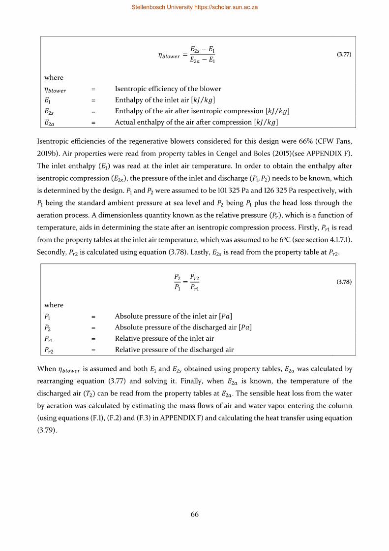
66

𝜂𝑏𝑙𝑜𝑤𝑒𝑟 =𝐸2𝑠 − 𝐸1

𝐸2𝑎 − 𝐸1 (3.77)

where

𝜂𝑏𝑙𝑜𝑤𝑒𝑟 = Isentropic efficiency of the blower

𝐸1 = Enthalpy of the inlet air [𝑘𝐽 𝑘𝑔⁄ ]

𝐸2𝑠 = Enthalpy of the air after isentropic compression [𝑘𝐽 𝑘𝑔⁄ ]

𝐸2𝑎 = Actual enthalpy of the air after compression [𝑘𝐽 𝑘𝑔⁄ ]

Isentropic efficiencies of the regenerative blowers considered for this design were 66% (CFW Fans,

2019b). Air properties were read from property tables in Cengel and Boles (2015)(see APPENDIX F).

The inlet enthalpy (𝐸1) was read at the inlet air temperature. In order to obtain the enthalpy after

isentropic compression (𝐸2𝑠), the pressure of the inlet and discharge (𝑃1, 𝑃2) needs to be known, which

is determined by the design. 𝑃1 and 𝑃2 were assumed to be 101 325 Pa and 126 325 Pa respectively, with

𝑃1 being the standard ambient pressure at sea level and 𝑃2 being 𝑃1 plus the head loss through the

aeration process. A dimensionless quantity known as the relative pressure (𝑃𝑟), which is a function of

temperature, aids in determining the state after an isentropic compression process. Firstly, 𝑃𝑟1 is read

from the property tables at the inlet air temperature, which was assumed to be 6oC (see section 4.1.7.1).

Secondly, 𝑃𝑟2 is calculated using equation (3.78). Lastly, 𝐸2𝑠 is read from the property table at 𝑃𝑟2.

𝑃2

𝑃1=

𝑃𝑟2

𝑃𝑟1 (3.78)

where

𝑃1 = Absolute pressure of the inlet air [𝑃𝑎]

𝑃2 = Absolute pressure of the discharged air [𝑃𝑎]

𝑃𝑟1 = Relative pressure of the inlet air

𝑃𝑟2 = Relative pressure of the discharged air

When 𝜂𝑏𝑙𝑜𝑤𝑒𝑟 is assumed and both 𝐸1 and 𝐸2𝑠 obtained using property tables, 𝐸2𝑎 was calculated by

rearranging equation (3.77) and solving it. Finally, when 𝐸2𝑎 is known, the temperature of the

discharged air (𝑇2) can be read from the property tables at 𝐸2𝑎. The sensible heat loss from the water

by aeration was calculated by estimating the mass flows of air and water vapor entering the column

(using equations (F.1), (F.2) and (F.3) in APPENDIX F) and calculating the heat transfer using equation

(3.79).


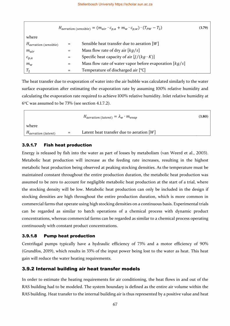
67

𝐻𝑎𝑒𝑟𝑎𝑡𝑖𝑜𝑛 (𝑠𝑒𝑛𝑠𝑖𝑏𝑙𝑒) = (𝑚𝑎𝑖𝑟 ∙ 𝑐𝑝,𝑎 + 𝑚𝑤 ∙ 𝑐𝑝,𝑤) ∙ (𝑇𝑃𝑊 − 𝑇2) (3.79)

where

𝐻𝑎𝑒𝑟𝑎𝑡𝑖𝑜𝑛 (𝑠𝑒𝑛𝑠𝑖𝑏𝑙𝑒) = Sensible heat transfer due to aeration [𝑊]

𝑚𝑎𝑖𝑟 = Mass flow rate of dry air [𝑘𝑔 𝑠⁄ ]

𝑐𝑝,𝑎 = Specific heat capacity of air [𝐽 (𝑘𝑔 ∙ 𝐾)⁄ ]

𝑚𝑤 = Mass flow rate of water vapor before evaporation [𝑘𝑔 𝑠⁄ ]

𝑇2 = Temperature of discharged air [℃]

The heat transfer due to evaporation of water into the air bubble was calculated similarly to the water

surface evaporation after estimating the evaporation rate by assuming 100% relative humidity and

calculating the evaporation rate required to achieve 100% relative humidity. Inlet relative humidity at

6oC was assumed to be 73% (see section 4.1.7.2).

𝐻𝑎𝑒𝑟𝑎𝑡𝑖𝑜𝑛 (𝑙𝑎𝑡𝑒𝑛𝑡) = 𝜆𝑤 ∙ 𝑚𝑒𝑣𝑎𝑝 (3.80)

where

𝐻𝑎𝑒𝑟𝑎𝑡𝑖𝑜𝑛 (𝑙𝑎𝑡𝑒𝑛𝑡) = Latent heat transfer due to aeration [𝑊]

3.9.1.7 Fish heat production

Energy is released by fish into the water as part of losses by metabolism (van Weerd et al., 2003).

Metabolic heat production will increase as the feeding rate increases, resulting in the highest

metabolic heat production being observed at peaking stocking densities. As the temperature must be

maintained constant throughout the entire production duration, the metabolic heat production was

assumed to be zero to account for negligible metabolic heat production at the start of a trial, where

the stocking density will be low. Metabolic heat production can only be included in the design if

stocking densities are high throughout the entire production duration, which is more common in

commercial farms that operate using high stocking densities on a continuous basis. Experimental trials

can be regarded as similar to batch operations of a chemical process with dynamic product

concentrations, whereas commercial farms can be regarded as similar to a chemical process operating

continuously with constant product concentrations.

3.9.1.8 Pump heat production

Centrifugal pumps typically have a hydraulic efficiency of 73% and a motor efficiency of 90%

(Grundfos, 2019), which results in 33% of the input power being lost to the water as heat. This heat

gain will reduce the water heating requirements.

3.9.2 Internal building air heat transfer models

In order to estimate the heating requirements for air conditioning, the heat flows in and out of the

RAS building had to be modeled. The system boundary is defined as the entire air volume within the

RAS building. Heat transfer to the internal building air is thus represented by a positive value and heat


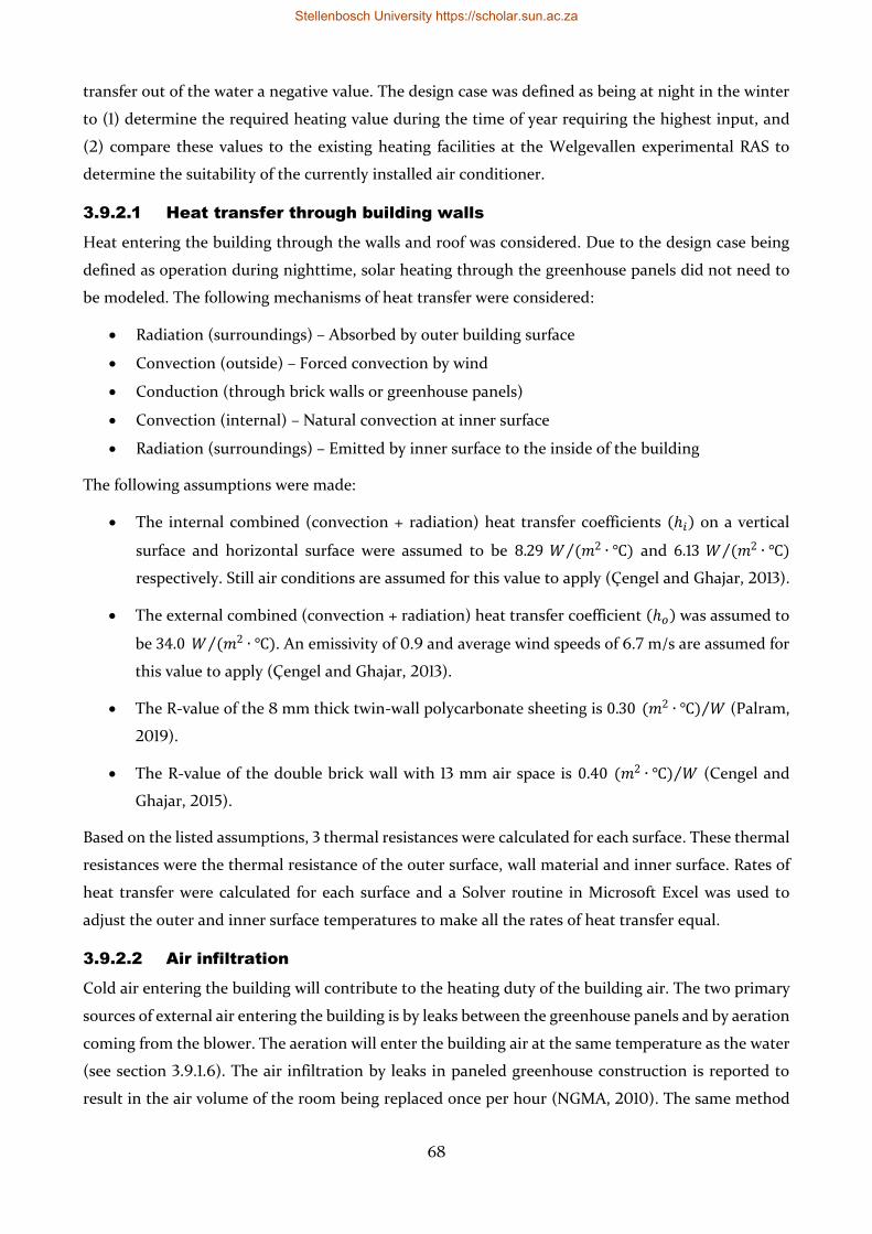
68

transfer out of the water a negative value. The design case was defined as being at night in the winter

to (1) determine the required heating value during the time of year requiring the highest input, and

(2) compare these values to the existing heating facilities at the Welgevallen experimental RAS to

determine the suitability of the currently installed air conditioner.

3.9.2.1 Heat transfer through building walls

Heat entering the building through the walls and roof was considered. Due to the design case being

defined as operation during nighttime, solar heating through the greenhouse panels did not need to

be modeled. The following mechanisms of heat transfer were considered:

• Radiation (surroundings) – Absorbed by outer building surface

• Convection (outside) – Forced convection by wind

• Conduction (through brick walls or greenhouse panels)

• Convection (internal) – Natural convection at inner surface

• Radiation (surroundings) – Emitted by inner surface to the inside of the building

The following assumptions were made:

• The internal combined (convection + radiation) heat transfer coefficients (ℎ𝑖) on a vertical

surface and horizontal surface were assumed to be 8.29 𝑊 (𝑚2 ∙ ℃)⁄ and 6.13 𝑊 (𝑚2 ∙ ℃)⁄

respectively. Still air conditions are assumed for this value to apply (Çengel and Ghajar, 2013).

• The external combined (convection + radiation) heat transfer coefficient (ℎ𝑜) was assumed to

be 34.0 𝑊 (𝑚2 ∙ ℃)⁄ . An emissivity of 0.9 and average wind speeds of 6.7 m/s are assumed for

this value to apply (Çengel and Ghajar, 2013).

• The R-value of the 8 mm thick twin-wall polycarbonate sheeting is 0.30 (𝑚2 ∙ ℃) 𝑊⁄ (Palram,

2019).

• The R-value of the double brick wall with 13 mm air space is 0.40 (𝑚2 ∙ ℃) 𝑊⁄ (Cengel and

Ghajar, 2015).

Based on the listed assumptions, 3 thermal resistances were calculated for each surface. These thermal

resistances were the thermal resistance of the outer surface, wall material and inner surface. Rates of

heat transfer were calculated for each surface and a Solver routine in Microsoft Excel was used to

adjust the outer and inner surface temperatures to make all the rates of heat transfer equal.

3.9.2.2 Air infiltration

Cold air entering the building will contribute to the heating duty of the building air. The two primary

sources of external air entering the building is by leaks between the greenhouse panels and by aeration

coming from the blower. The aeration will enter the building air at the same temperature as the water

(see section 3.9.1.6). The air infiltration by leaks in paneled greenhouse construction is reported to

result in the air volume of the room being replaced once per hour (NGMA, 2010). The same method


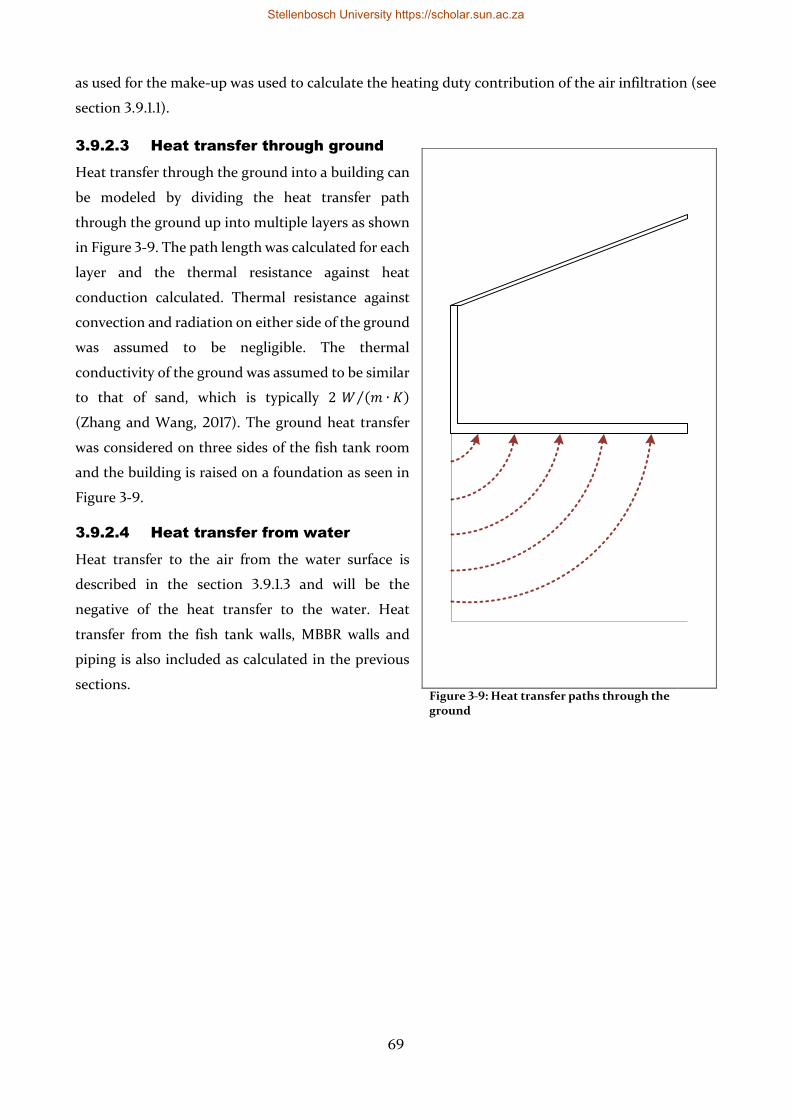
69

as used for the make-up was used to calculate the heating duty contribution of the air infiltration (see

section 3.9.1.1).

3.9.2.3 Heat transfer through ground

Heat transfer through the ground into a building can

be modeled by dividing the heat transfer path

through the ground up into multiple layers as shown

in Figure 3-9. The path length was calculated for each

layer and the thermal resistance against heat

conduction calculated. Thermal resistance against

convection and radiation on either side of the ground

was assumed to be negligible. The thermal

conductivity of the ground was assumed to be similar

to that of sand, which is typically 2 𝑊 (𝑚 ∙ 𝐾)⁄

(Zhang and Wang, 2017). The ground heat transfer

was considered on three sides of the fish tank room

and the building is raised on a foundation as seen in

Figure 3-9.

3.9.2.4 Heat transfer from water

Heat transfer to the air from the water surface is

described in the section 3.9.1.3 and will be the

negative of the heat transfer to the water. Heat

transfer from the fish tank walls, MBBR walls and

piping is also included as calculated in the previous

sections.

Figure 3-9: Heat transfer paths through the ground


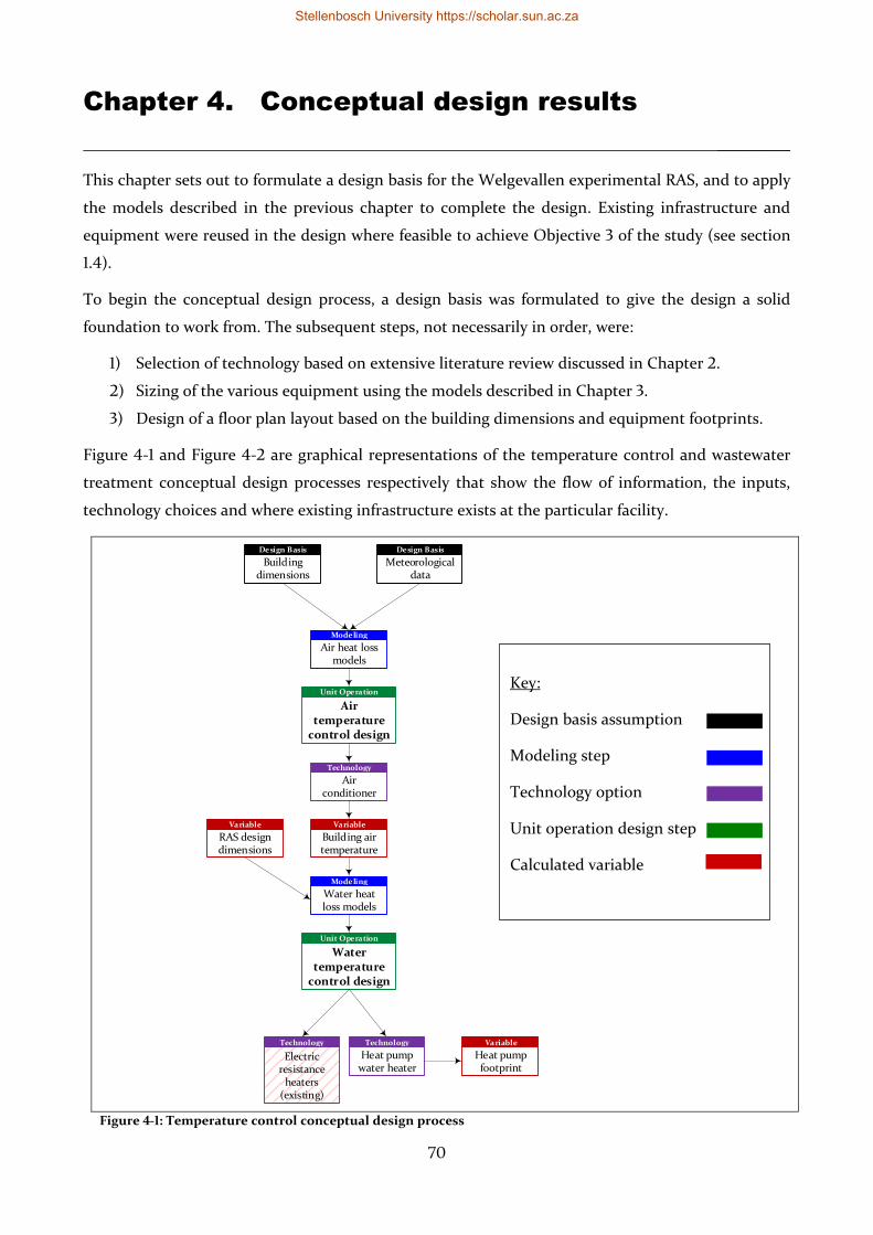
70

Chapter 4. Conceptual design results

_________

This chapter sets out to formulate a design basis for the Welgevallen experimental RAS, and to apply

the models described in the previous chapter to complete the design. Existing infrastructure and

equipment were reused in the design where feasible to achieve Objective 3 of the study (see section

1.4).

To begin the conceptual design process, a design basis was formulated to give the design a solid

foundation to work from. The subsequent steps, not necessarily in order, were:

1) Selection of technology based on extensive literature review discussed in Chapter 2.

2) Sizing of the various equipment using the models described in Chapter 3.

3) Design of a floor plan layout based on the building dimensions and equipment footprints.

Figure 4-1 and Figure 4-2 are graphical representations of the temperature control and wastewater

treatment conceptual design processes respectively that show the flow of information, the inputs,

technology choices and where existing infrastructure exists at the particular facility.

Figure 4-1: Temperature control conceptual design process

Design Basis

Building dimensions

Water temperature

control design

Unit Operation

Air temperature

control design

Unit Operation

Modeling

Air heat loss models

Technology

Heat pump water heater

Technology

Air conditioner

Design Basis

Meteorological data

Variable

Building air temperature

Technology

Electric resistance

heaters (existing)

Modeling

Water heat loss models

Variable

RAS design dimensions

Variable

Heat pump footprint

Key:

Design basis assumption

Modeling step

Technology option

Unit operation design step

Calculated variable


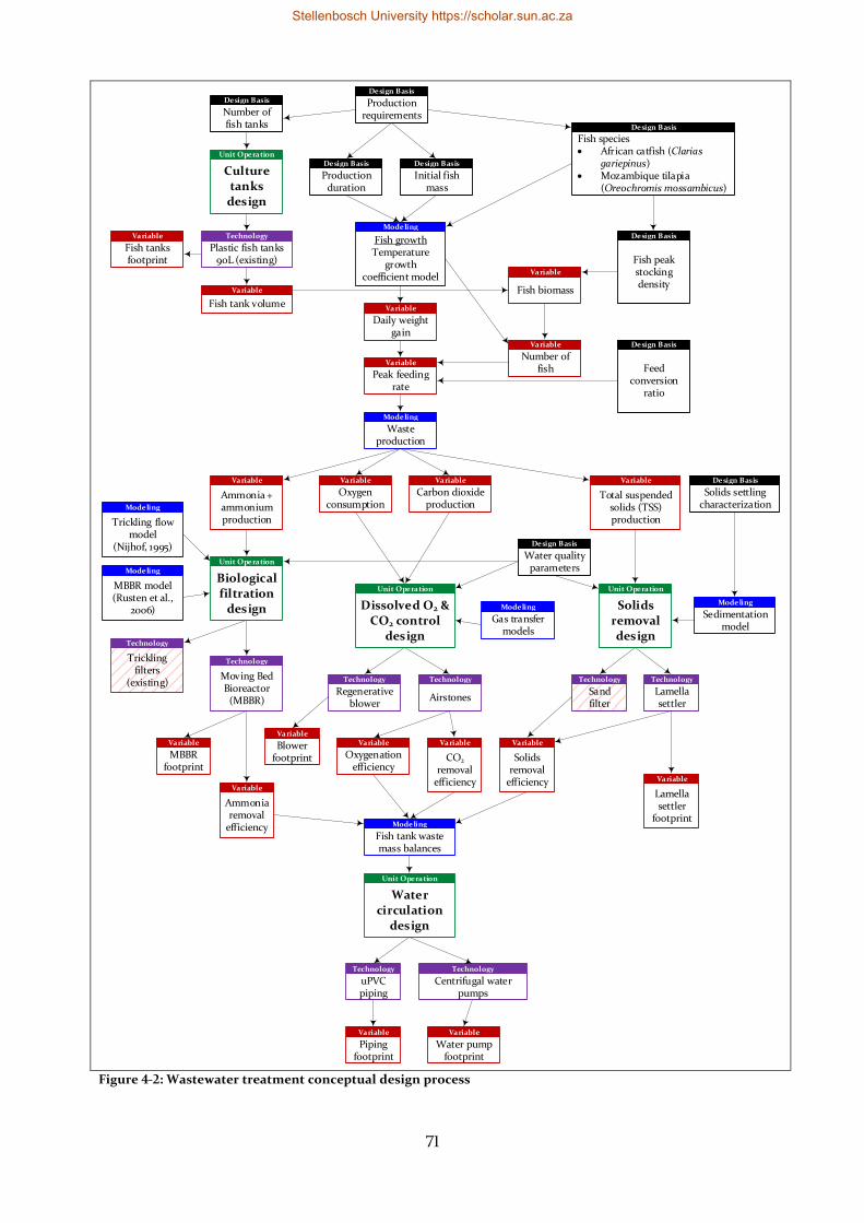
71

Figure 4-2: Wastewater treatment conceptual design process

Design Basis

Number of fish tanks

Design Basis

Production duration

Design Basis

Initial fish mass

Design Basis

Water quality parameters

Design Basis

Production requirements

Variable

Fish biomass

Technology

Plastic fish tanks 90L (existing)

Modeling

Waste production

Technology

Sand filter

Technology

Lamella settler

Variable

Oxygen consumption

Variable

Carbon dioxide production

Design Basis

Solids settling characterization

Variable

Total suspended solids (TSS) production

Design Basis

Fish species• African catfish (Clarias

gariepinus)• Mozambique tilapia

(Oreochromis mossambicus)

Modeling

Gas transfer models

Modeling

Sedimentation model

Technology

Regenerative blower

Technology

Airstones

Modeling

Fish tank waste mass balances

Variable

MBBR footprint

Variable

Oxygenation efficiency

Technology

Centrifugal water pumps

Variable

Water pump footprint

Technology

uPVC piping

Variable

Piping footprint

Variable

Fish tanks footprint

Variable

Blower footprint

Biological filtration

design

Unit Operation

Dissolved O2 & CO2 control

design

Unit Operation

Solids removal design

Unit Operation

Water circulation

design

Unit Operation

Culture tanks

design

Unit Operation

Modeling

Trickling flow model

(Nijhof, 1995)

Modeling

MBBR model(Rusten et al.,

2006)

Variable

Ammonia + ammonium production

Technology

Moving Bed Bioreactor (MBBR)

Technology

Trickling filters

(existing)

Variable

Ammonia removal

efficiency

Variable

CO2 removal

efficiency

Variable

Solids removal

efficiency Variable

Lamella settler

footprint

Variable

Daily weight gain

Modeling

Fish growth Temperature

growth coefficient model

Variable

Peak feeding rate

Variable

Number of fish

Design Basis

Fish peak stocking density

Design Basis

Feed conversion

ratio

Variable

Fish tank volume


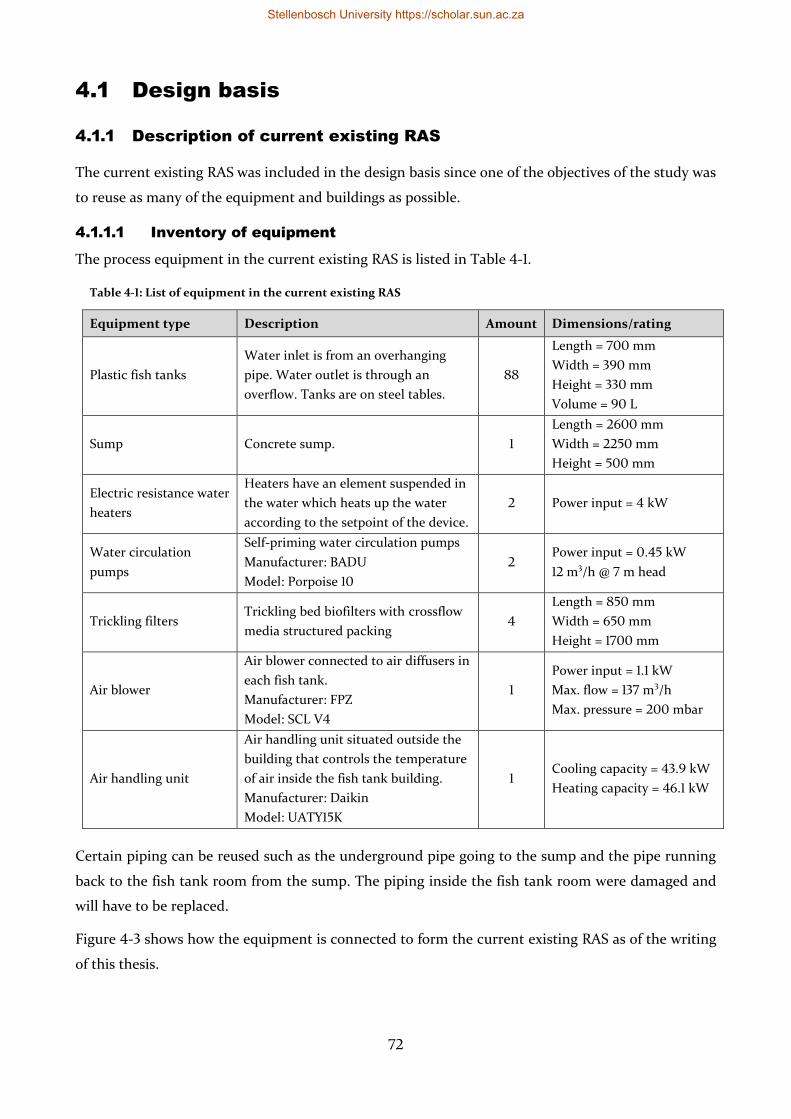
72

4.1 Design basis

4.1.1 Description of current existing RAS

The current existing RAS was included in the design basis since one of the objectives of the study was

to reuse as many of the equipment and buildings as possible.

4.1.1.1 Inventory of equipment

The process equipment in the current existing RAS is listed in Table 4-1.

Table 4-1: List of equipment in the current existing RAS

Equipment type Description Amount Dimensions/rating

Plastic fish tanks

Water inlet is from an overhanging

pipe. Water outlet is through an

overflow. Tanks are on steel tables.

88

Length = 700 mm

Width = 390 mm

Height = 330 mm

Volume = 90 L

Sump Concrete sump. 1

Length = 2600 mm

Width = 2250 mm

Height = 500 mm

Electric resistance water

heaters

Heaters have an element suspended in

the water which heats up the water

according to the setpoint of the device.

2 Power input = 4 kW

Water circulation

pumps

Self-priming water circulation pumps

Manufacturer: BADU

Model: Porpoise 10

2 Power input = 0.45 kW

12 m3/h @ 7 m head

Trickling filters Trickling bed biofilters with crossflow

media structured packing 4

Length = 850 mm

Width = 650 mm

Height = 1700 mm

Air blower

Air blower connected to air diffusers in

each fish tank.

Manufacturer: FPZ

Model: SCL V4

1

Power input = 1.1 kW

Max. flow = 137 m3/h

Max. pressure = 200 mbar

Air handling unit

Air handling unit situated outside the

building that controls the temperature

of air inside the fish tank building.

Manufacturer: Daikin

Model: UATY15K

1 Cooling capacity = 43.9 kW

Heating capacity = 46.1 kW

Certain piping can be reused such as the underground pipe going to the sump and the pipe running

back to the fish tank room from the sump. The piping inside the fish tank room were damaged and

will have to be replaced.

Figure 4-3 shows how the equipment is connected to form the current existing RAS as of the writing

of this thesis.


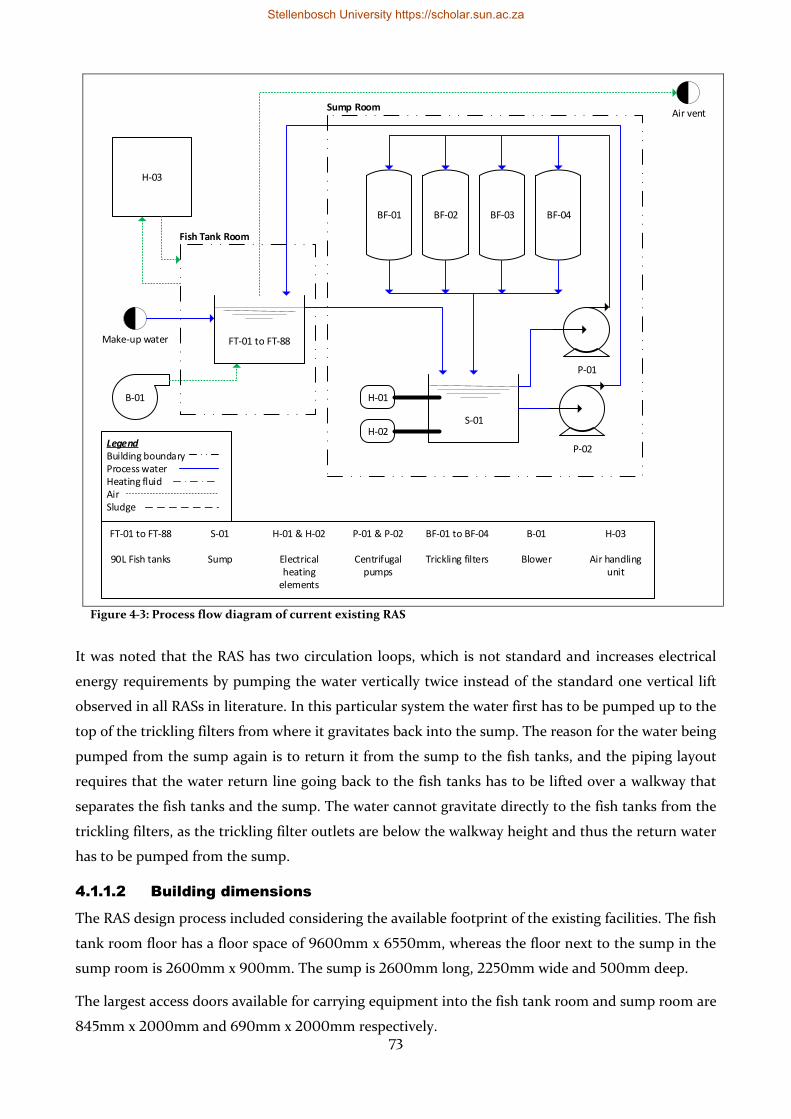
73

Figure 4-3: Process flow diagram of current existing RAS

It was noted that the RAS has two circulation loops, which is not standard and increases electrical

energy requirements by pumping the water vertically twice instead of the standard one vertical lift

observed in all RASs in literature. In this particular system the water first has to be pumped up to the

top of the trickling filters from where it gravitates back into the sump. The reason for the water being

pumped from the sump again is to return it from the sump to the fish tanks, and the piping layout

requires that the water return line going back to the fish tanks has to be lifted over a walkway that

separates the fish tanks and the sump. The water cannot gravitate directly to the fish tanks from the

trickling filters, as the trickling filter outlets are below the walkway height and thus the return water

has to be pumped from the sump.

4.1.1.2 Building dimensions

The RAS design process included considering the available footprint of the existing facilities. The fish

tank room floor has a floor space of 9600mm x 6550mm, whereas the floor next to the sump in the

sump room is 2600mm x 900mm. The sump is 2600mm long, 2250mm wide and 500mm deep.

The largest access doors available for carrying equipment into the fish tank room and sump room are

845mm x 2000mm and 690mm x 2000mm respectively.

FT-01 to FT-88

BF-01

FT-01 to FT-88

90L Fish tanks

BF-01 to BF-04

Trickling filters

BF-02 BF-03 BF-04

H-01 & H-02

Electrical heating

elements

S-01

P-01

P-02

S-01

Sump

H-01

H-02

P-01 & P-02

Centrifugal pumps

B-01

Blower

Make-up water

B-01

Air vent

H-03

LegendBuilding boundaryProcess waterHeating fluidAirSludge

H-03

Air handling unit

Fish Tank Room

Sump Room


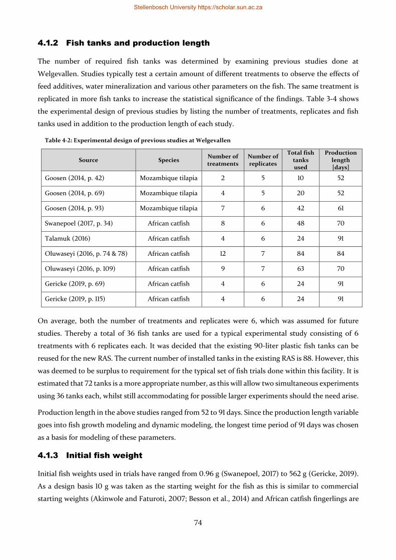
74

4.1.2 Fish tanks and production length

The number of required fish tanks was determined by examining previous studies done at

Welgevallen. Studies typically test a certain amount of different treatments to observe the effects of

feed additives, water mineralization and various other parameters on the fish. The same treatment is

replicated in more fish tanks to increase the statistical significance of the findings. Table 3-4 shows

the experimental design of previous studies by listing the number of treatments, replicates and fish

tanks used in addition to the production length of each study.

Table 4-2: Experimental design of previous studies at Welgevallen

Source Species Number of treatments

Number of replicates

Total fish tanks used

Production length [days]

Goosen (2014, p. 42) Mozambique tilapia 2 5 10 52



Swanepoel (2017, p. 34) African catfish 8 6 48 70

Talamuk (2016) African catfish 4 6 24 91

Oluwaseyi (2016, p. 74 & 78) African catfish 12 7 84 84

Oluwaseyi (2016, p. 109) African catfish 9 7 63 70

Gericke (2019, p. 69) African catfish 4 6 24 91

Gericke (2019, p. 115) African catfish 4 6 24 91

On average, both the number of treatments and replicates were 6, which was assumed for future

studies. Thereby a total of 36 fish tanks are used for a typical experimental study consisting of 6

treatments with 6 replicates each. It was decided that the existing 90-liter plastic fish tanks can be

reused for the new RAS. The current number of installed tanks in the existing RAS is 88. However, this

was deemed to be surplus to requirement for the typical set of fish trials done within this facility. It is

estimated that 72 tanks is a more appropriate number, as this will allow two simultaneous experiments

using 36 tanks each, whilst still accommodating for possible larger experiments should the need arise.

Production length in the above studies ranged from 52 to 91 days. Since the production length variable

goes into fish growth modeling and dynamic modeling, the longest time period of 91 days was chosen

as a basis for modeling of these parameters.

4.1.3 Initial fish weight

Initial fish weights used in trials have ranged from 0.96 g (Swanepoel, 2017) to 562 g (Gericke, 2019).

As a design basis 10 g was taken as the starting weight for the fish as this is similar to commercial

starting weights (Akinwole and Faturoti, 2007; Besson et al., 2014) and African catfish fingerlings are


75

widely available for purchase at 10 g from commercial hatcheries, to be used in trials. 10 g African

catfish has also been used in a study at Welgevallen (Oluwaseyi, 2016).

4.1.4 Stocking density

Fish stocking density, defined as kg fish per m3 of tank volume, is a critical parameter dictating the

design, as it influences the amount of feed given per day and hence the waste production rates. As is

standard for experimental RAS systems, the experimental trials to be done using the RAS will stock a

fixed number of fish at the start and observe growth over time with minimal exchange of fish during

the experiment. Fish that are removed from the system for sampling purposes are replaced to maintain

the biomass in the trial. Thus, the stocking density within the RAS will increase as biomass increases,

and the peak stocking density will be observed at the end of the trial due to fish growth. Trials should

preferably be done at stocking densities close to that of commercial systems to eliminate stocking

density effects on the results if applied in industry.

An intensive tilapia RAS in the USA is reported to operate at 82 kg/m3 (Watanabe et al., 2002). A

guide for recirculating aquaculture reported commercial stocking densities for tilapia of 20 to 120

kg/m3 (Negroni, 2013). Table 4-3 shows allowable stocking densities reported for tilapia (Timmons

and Ebeling, 2007, p. 121).

Table 4-3: Allowable stocking densities for tilapia RAS culture at different fish masses (Timmons and Ebeling, 2007, p. 121)

Fish mass [g] Allowable stocking density [kg/m3]

0.2 8.4

1.4 17

11 34

38 50

75 63

83 83

346 105

599 126

951 147

African catfish RAS culture in the Netherlands is typically done in two phases. Phase 1 grows 10g fish

to a mass of 150g at peak stocking densities between 100 and 300 kg/m3. Phase 2 grows 150g fish to a

mass of 1500g which is suitable for market consumption. Phase 2 has peak stocking densities between

200 and 500 kg/m3 (van de Nieuwegiessen et al., 2009, 2008). An African catfish RAS in Nigeria

reported rearing adult fish at 176.6 kg/m3 (Akinwole and Faturoti, 2007). A guide for recirculating

aquaculture reported commercial stocking densities for African catfish of 300 kg/m3 (Negroni, 2013).

A semi-commercial experimental African catfish RAS in Germany operated at intensive aquaculture

conditions with a stocking density of 200 kg/m3 (Strauch et al., 2018).


76

Based on the above information, the first design iteration designed a RAS for an African catfish peak

stocking density of 200 kg/m3. Commercial tilapia peak stocking densities are considerably lower than

that of African catfish. If operated at a peak stocking density of 200 kg/m3, the new RAS would

represent the conditions of commercial farms. However, after several iterations in the design process,

it became apparent that the biofiltration demands of operating the RAS at a commercial stocking

density of 200 kg/m3 exceeded the existing floor space of the Welgevallen experimental facilities.

Consequently, the design stocking density was reduced to 50 kg/m3. This implied that the RAS was to

be designed for utilization of all tanks at a peak stocking density of 50 kg/m3. If the researchers desire

to operate at a peak stocking density of 200 kg/m3, only a quarter of the tank need to be used to

achieve the same peak biomass and feeding rate for which the RAS was designed.

4.1.5 Feed composition and feeding rate

Feed composition and feeding rate have a large influence on waste production and therefore need to

be carefully determined. Particularly the protein content of the feed is important, as it is the main

source of nitrogenous wastes produced in the RAS. Feed protein content was assumed to be 45% (see

section 3.3.1). The remaining feed components were assumed to be that of a typical fish feed (Wik and

Lindén, 2004) and are listed in Table 4-4.

Table 4-4: Fish feed composition

Component Feed content [g/g feed]

Protein 0.45

Carbohydrates 0.14

Fat 0.24

Ash 0.08

Water 0.09

A feed conversion ratio (FCR) of 1.5 has been chosen to model the feeding rate (see section 3.2.4). The

maximum feeding rate was estimated to be 10.3 kg/day under the assumption of operating all tanks

simultaneously, at conditions that will result in the maximum allowable stocking density to be reached

at the last day of a 91-day growth trial. A peak stocking density of 50 kg/m3 was used. Figure 4-4 shows

the estimated daily feeding rate of each day of production.


77

Figure 4-4: Total estimated daily feeding rate over time

From Figure 4-4 it was observed that the peak daily feeding rate is experienced at the end of a

production period, as is expected.

4.1.6 Water quality

The target design water quality parameters suitable for both African catfish and tilapia motivated in

section 2.1 are given in Table 4-5.

Table 4-5: Chosen design water quality parameters for rearing tilapia and African catfish

Water quality parameter Limit

Dissolved oxygen [mg/L] > 4; optimal = 5

Temperature [oC] 27oC ±1 oC

NH3-N [mg/L] < 0.06

TAN [mg/L] < 3.0

NO2-N [mg/L] < 1.0

NO3-N [mg/L] < 140

pH 7.0 ±0.2

Alkalinity [mg equiv. CaCO3/L] Will depend on CO2 production

Hardness [mg equiv. CaCO3/L] > 100

Dissolved CO2 [mg/L] < 15 (rough guideline)

Salinity [ppm] 2000 - 3000

TSS [mg/L] < 25; optimally < 10

BOD5 [mg/L] < 110

4.1.7 Meteorological data

Meteorological data such as air temperatures and humidity were required as inputs for the energy

balance calculations. The meteorological station closest to the Welgevallen site was a solar radiation

monitoring station at Stellenbosch University (SAURAN, 2019).


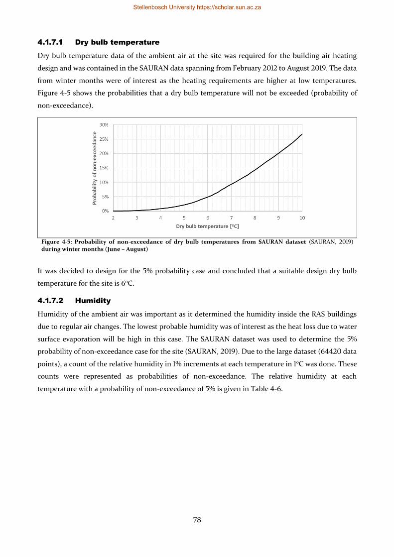
78

4.1.7.1 Dry bulb temperature

Dry bulb temperature data of the ambient air at the site was required for the building air heating

design and was contained in the SAURAN data spanning from February 2012 to August 2019. The data

from winter months were of interest as the heating requirements are higher at low temperatures.

Figure 4-5 shows the probabilities that a dry bulb temperature will not be exceeded (probability of

non-exceedance).

Figure 4-5: Probability of non-exceedance of dry bulb temperatures from SAURAN dataset (SAURAN, 2019) during winter months (June – August)

It was decided to design for the 5% probability case and concluded that a suitable design dry bulb

temperature for the site is 6oC.

4.1.7.2 Humidity

Humidity of the ambient air was important as it determined the humidity inside the RAS buildings

due to regular air changes. The lowest probable humidity was of interest as the heat loss due to water

surface evaporation will be high in this case. The SAURAN dataset was used to determine the 5%

probability of non-exceedance case for the site (SAURAN, 2019). Due to the large dataset (64420 data

points), a count of the relative humidity in 1% increments at each temperature in 1oC was done. These

counts were represented as probabilities of non-exceedance. The relative humidity at each

temperature with a probability of non-exceedance of 5% is given in Table 4-6.


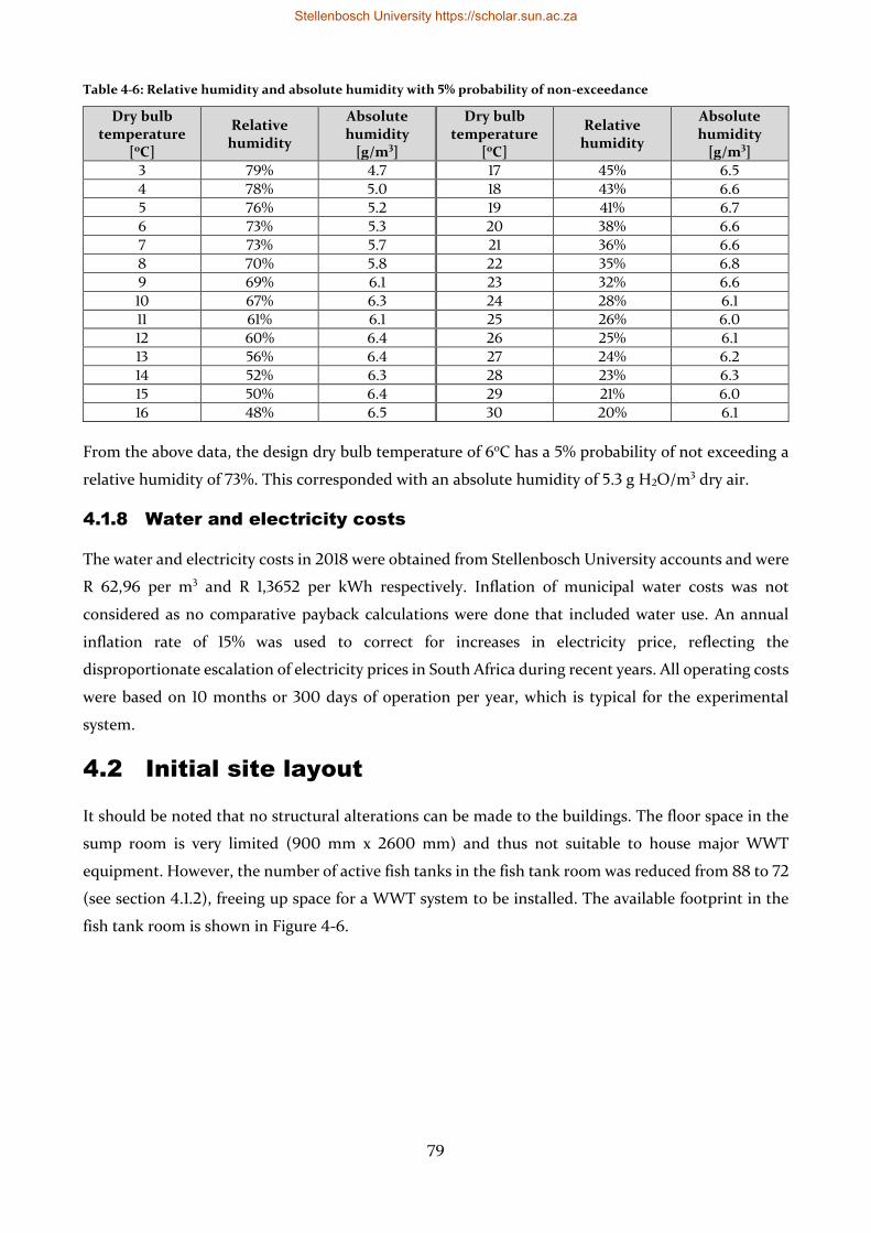
79

Table 4-6: Relative humidity and absolute humidity with 5% probability of non-exceedance

Dry bulb temperature

[oC]

Relative humidity

Absolute humidity

[g/m3]

Dry bulb temperature

[oC]

Relative humidity

Absolute humidity

[g/m3]

3 79% 4.7 17 45% 6.5

4 78% 5.0 18 43% 6.6

5 76% 5.2 19 41% 6.7

6 73% 5.3 20 38% 6.6

7 73% 5.7 21 36% 6.6

8 70% 5.8 22 35% 6.8

9 69% 6.1 23 32% 6.6

10 67% 6.3 24 28% 6.1

11 61% 6.1 25 26% 6.0

12 60% 6.4 26 25% 6.1

13 56% 6.4 27 24% 6.2

14 52% 6.3 28 23% 6.3

15 50% 6.4 29 21% 6.0

16 48% 6.5 30 20% 6.1

From the above data, the design dry bulb temperature of 6oC has a 5% probability of not exceeding a

relative humidity of 73%. This corresponded with an absolute humidity of 5.3 g H2O/m3 dry air.

4.1.8 Water and electricity costs

The water and electricity costs in 2018 were obtained from Stellenbosch University accounts and were

R 62,96 per m3 and R 1,3652 per kWh respectively. Inflation of municipal water costs was not

considered as no comparative payback calculations were done that included water use. An annual

inflation rate of 15% was used to correct for increases in electricity price, reflecting the

disproportionate escalation of electricity prices in South Africa during recent years. All operating costs

were based on 10 months or 300 days of operation per year, which is typical for the experimental

system.

4.2 Initial site layout

It should be noted that no structural alterations can be made to the buildings. The floor space in the

sump room is very limited (900 mm x 2600 mm) and thus not suitable to house major WWT

equipment. However, the number of active fish tanks in the fish tank room was reduced from 88 to 72

(see section 4.1.2), freeing up space for a WWT system to be installed. The available footprint in the

fish tank room is shown in Figure 4-6.


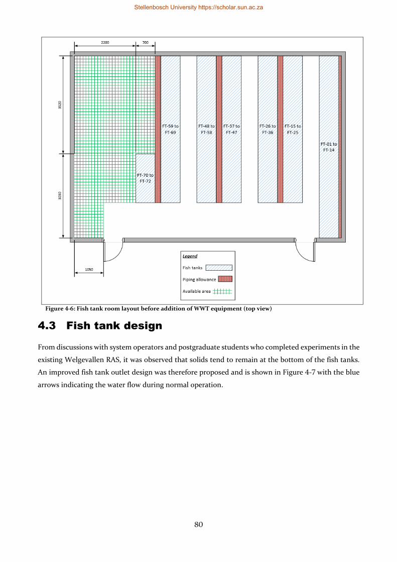
80

Figure 4-6: Fish tank room layout before addition of WWT equipment (top view)

4.3 Fish tank design

From discussions with system operators and postgraduate students who completed experiments in the

existing Welgevallen RAS, it was observed that solids tend to remain at the bottom of the fish tanks.

An improved fish tank outlet design was therefore proposed and is shown in Figure 4-7 with the blue

arrows indicating the water flow during normal operation.


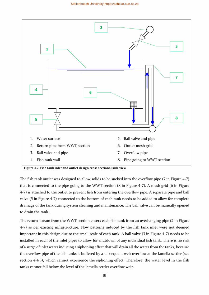
81

1. Water surface

2. Return pipe from WWT section

3. Ball valve and pipe

4. Fish tank wall

5. Ball valve and pipe

6. Outlet mesh grid

7. Overflow pipe

8. Pipe going to WWT section

Figure 4-7: Fish tank inlet and outlet design cross sectional side view

The fish tank outlet was designed to allow solids to be sucked into the overflow pipe (7 in Figure 4-7)

that is connected to the pipe going to the WWT section (8 in Figure 4-7). A mesh grid (6 in Figure

4-7) is attached to the outlet to prevent fish from entering the overflow pipe. A separate pipe and ball

valve (5 in Figure 4-7) connected to the bottom of each tank needs to be added to allow for complete

drainage of the tank during system cleaning and maintenance. The ball valve can be manually opened

to drain the tank.

The return stream from the WWT section enters each fish tank from an overhanging pipe (2 in Figure

4-7) as per existing infrastructure. Flow patterns induced by the fish tank inlet were not deemed

important in this design due to the small scale of each tank. A ball valve (3 in Figure 4-7) needs to be

installed in each of the inlet pipes to allow for shutdown of any individual fish tank. There is no risk

of a surge of inlet water inducing a siphoning effect that will drain all the water from the tanks, because

the overflow pipe of the fish tanks is buffered by a subsequent weir overflow at the lamella settler (see

section 4.4.3), which cannot experience the siphoning effect. Therefore, the water level in the fish

tanks cannot fall below the level of the lamella settler overflow weir.


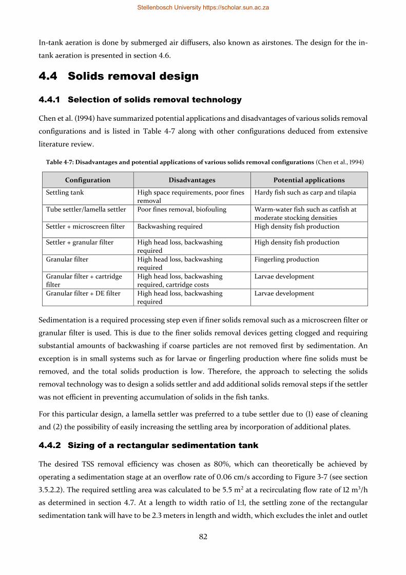
82

In-tank aeration is done by submerged air diffusers, also known as airstones. The design for the in-

tank aeration is presented in section 4.6.

4.4 Solids removal design

4.4.1 Selection of solids removal technology

Chen et al. (1994) have summarized potential applications and disadvantages of various solids removal

configurations and is listed in Table 4-7 along with other configurations deduced from extensive

literature review.

Table 4-7: Disadvantages and potential applications of various solids removal configurations (Chen et al., 1994)

Configuration Disadvantages Potential applications

Settling tank High space requirements, poor fines removal

Hardy fish such as carp and tilapia

Tube settler/lamella settler Poor fines removal, biofouling Warm-water fish such as catfish at moderate stocking densities

Settler + microscreen filter Backwashing required High density fish production

Settler + granular filter High head loss, backwashing required

High density fish production

Granular filter High head loss, backwashing required

Fingerling production

Granular filter + cartridge filter

High head loss, backwashing required, cartridge costs

Larvae development

Granular filter + DE filter High head loss, backwashing required

Larvae development

Sedimentation is a required processing step even if finer solids removal such as a microscreen filter or

granular filter is used. This is due to the finer solids removal devices getting clogged and requiring

substantial amounts of backwashing if coarse particles are not removed first by sedimentation. An

exception is in small systems such as for larvae or fingerling production where fine solids must be

removed, and the total solids production is low. Therefore, the approach to selecting the solids

removal technology was to design a solids settler and add additional solids removal steps if the settler

was not efficient in preventing accumulation of solids in the fish tanks.

For this particular design, a lamella settler was preferred to a tube settler due to (1) ease of cleaning

and (2) the possibility of easily increasing the settling area by incorporation of additional plates.

4.4.2 Sizing of a rectangular sedimentation tank

The desired TSS removal efficiency was chosen as 80%, which can theoretically be achieved by

operating a sedimentation stage at an overflow rate of 0.06 cm/s according to Figure 3-7 (see section

3.5.2.2). The required settling area was calculated to be 5.5 m2 at a recirculating flow rate of 12 m3/h

as determined in section 4.7. At a length to width ratio of 1:1, the settling zone of the rectangular

sedimentation tank will have to be 2.3 meters in length and width, which excludes the inlet and outlet


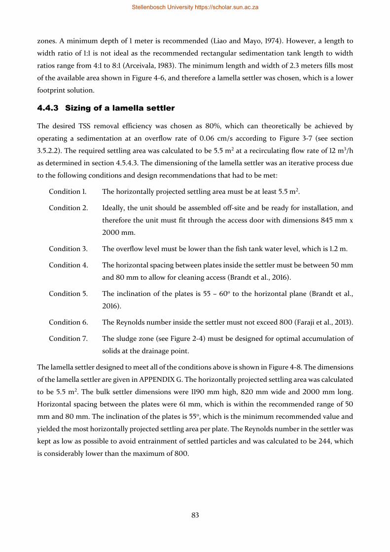
83

zones. A minimum depth of 1 meter is recommended (Liao and Mayo, 1974). However, a length to

width ratio of 1:1 is not ideal as the recommended rectangular sedimentation tank length to width

ratios range from 4:1 to 8:1 (Arceivala, 1983). The minimum length and width of 2.3 meters fills most

of the available area shown in Figure 4-6, and therefore a lamella settler was chosen, which is a lower

footprint solution.

4.4.3 Sizing of a lamella settler

The desired TSS removal efficiency was chosen as 80%, which can theoretically be achieved by

operating a sedimentation at an overflow rate of 0.06 cm/s according to Figure 3-7 (see section

3.5.2.2). The required settling area was calculated to be 5.5 m2 at a recirculating flow rate of 12 m3/h

as determined in section 4.5.4.3. The dimensioning of the lamella settler was an iterative process due

to the following conditions and design recommendations that had to be met:

Condition 1. The horizontally projected settling area must be at least 5.5 m2.

Condition 2. Ideally, the unit should be assembled off-site and be ready for installation, and

therefore the unit must fit through the access door with dimensions 845 mm x

2000 mm.

Condition 3. The overflow level must be lower than the fish tank water level, which is 1.2 m.

Condition 4. The horizontal spacing between plates inside the settler must be between 50 mm

and 80 mm to allow for cleaning access (Brandt et al., 2016).

Condition 5. The inclination of the plates is 55 – 60o to the horizontal plane (Brandt et al.,

2016).

Condition 6. The Reynolds number inside the settler must not exceed 800 (Faraji et al., 2013).

Condition 7. The sludge zone (see Figure 2-4) must be designed for optimal accumulation of

solids at the drainage point.

The lamella settler designed to meet all of the conditions above is shown in Figure 4-8. The dimensions

of the lamella settler are given in APPENDIX G. The horizontally projected settling area was calculated

to be 5.5 m2. The bulk settler dimensions were 1190 mm high, 820 mm wide and 2000 mm long.

Horizontal spacing between the plates were 61 mm, which is within the recommended range of 50

mm and 80 mm. The inclination of the plates is 55o, which is the minimum recommended value and

yielded the most horizontally projected settling area per plate. The Reynolds number in the settler was

kept as low as possible to avoid entrainment of settled particles and was calculated to be 244, which

is considerably lower than the maximum of 800.


84

1. Water inlet from fish tank overflow

2. Lamella plates

3. Water surface

4. Overflow weir

5. Water outlet to sump

6. Sludge collection cone

7. Water drainpipe for maintenance

8. Water drain ball valve for maintenance

9. Sludge flushing tap

10. Sludge flushing collection point

Figure 4-8: Lamella settler drawing

The flow hydraulics between the fish tanks and the settler was assessed to ensure that water level

remains at the overflow level. If the head loss through the connecting piping is more than the

difference in overflow levels, the water will accumulate in the fish tanks until the head loss is equal to

the height difference between the water levels. The fish tank furthest from the settler was assessed as

it will have the flow with the most head loss. After adjusting the pipe sizes, it was estimated that the

minimum elevation difference between the fish tank overflows and the settler overflow should be 32

mm. A decrease in specified pipe sizes will result in a rise in water levels in the fish tanks and possibly

complete overflow. Therefore, it is critical to construct the system as specified.

11

2

3

4

5

6

78

9

10


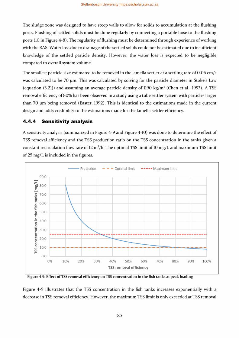
85

The sludge zone was designed to have steep walls to allow for solids to accumulation at the flushing

ports. Flushing of settled solids must be done regularly by connecting a portable hose to the flushing

ports (10 in Figure 4-8). The regularity of flushing must be determined through experience of working

with the RAS. Water loss due to drainage of the settled solids could not be estimated due to insufficient

knowledge of the settled particle density. However, the water loss is expected to be negligible

compared to overall system volume.

The smallest particle size estimated to be removed in the lamella settler at a settling rate of 0.06 cm/s

was calculated to be 70 μm. This was calculated by solving for the particle diameter in Stoke’s Law

(equation (3.21)) and assuming an average particle density of 1190 kg/m3 (Chen et al., 1993). A TSS

removal efficiency of 80% has been observed in a study using a tube settler system with particles larger

than 70 μm being removed (Easter, 1992). This is identical to the estimations made in the current

design and adds credibility to the estimations made for the lamella settler efficiency.

4.4.4 Sensitivity analysis

A sensitivity analysis (summarized in Figure 4-9 and Figure 4-10) was done to determine the effect of

TSS removal efficiency and the TSS production ratio on the TSS concentration in the tanks given a

constant recirculation flow rate of 12 m3/h. The optimal TSS limit of 10 mg/L and maximum TSS limit

of 25 mg/L is included in the figures.

Figure 4-9: Effect of TSS removal efficiency on TSS concentration in the fish tanks at peak loading

Figure 4-9 illustrates that the TSS concentration in the fish tanks increases exponentially with a

decrease in TSS removal efficiency. However, the maximum TSS limit is only exceeded at TSS removal


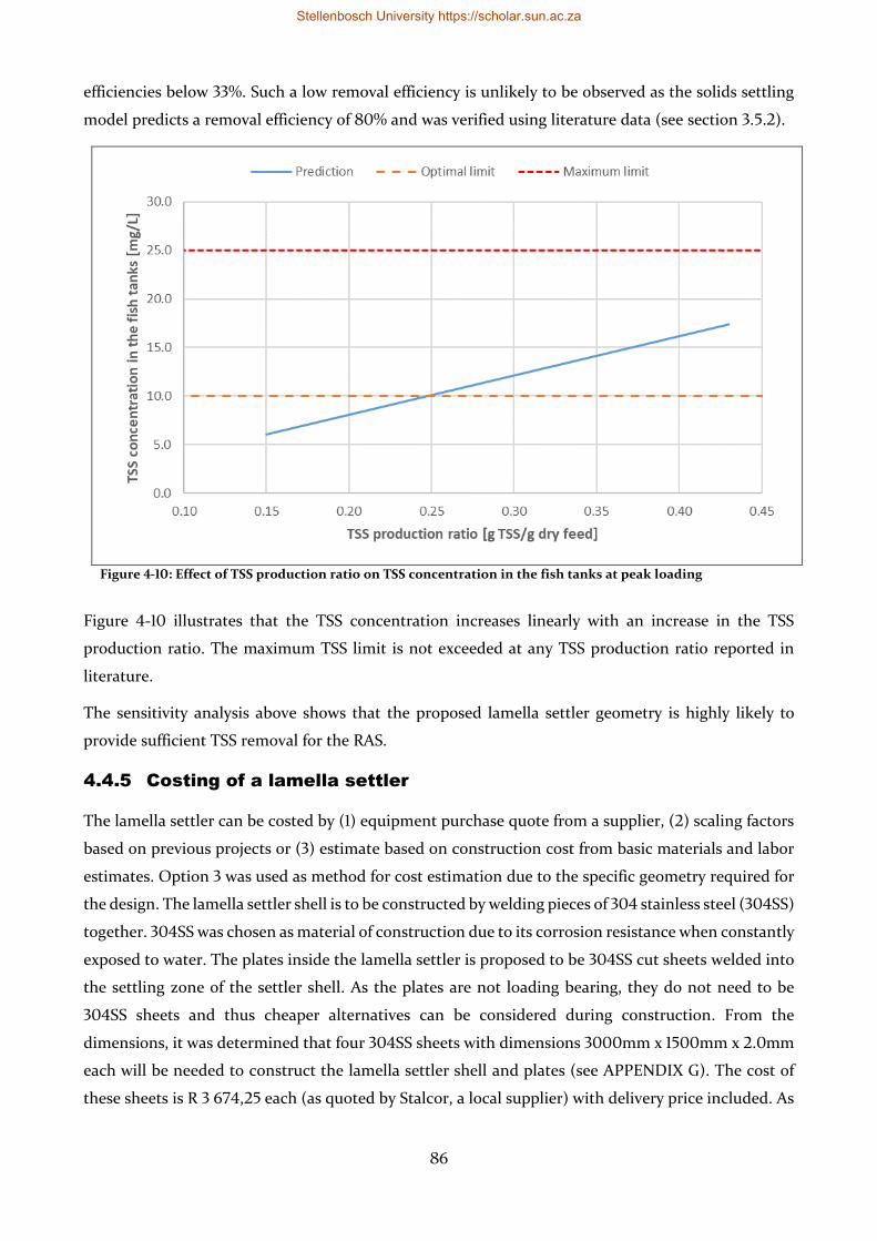
86

efficiencies below 33%. Such a low removal efficiency is unlikely to be observed as the solids settling

model predicts a removal efficiency of 80% and was verified using literature data (see section 3.5.2).

Figure 4-10: Effect of TSS production ratio on TSS concentration in the fish tanks at peak loading

Figure 4-10 illustrates that the TSS concentration increases linearly with an increase in the TSS

production ratio. The maximum TSS limit is not exceeded at any TSS production ratio reported in

literature.

The sensitivity analysis above shows that the proposed lamella settler geometry is highly likely to

provide sufficient TSS removal for the RAS.

4.4.5 Costing of a lamella settler

The lamella settler can be costed by (1) equipment purchase quote from a supplier, (2) scaling factors

based on previous projects or (3) estimate based on construction cost from basic materials and labor

estimates. Option 3 was used as method for cost estimation due to the specific geometry required for

the design. The lamella settler shell is to be constructed by welding pieces of 304 stainless steel (304SS)

together. 304SS was chosen as material of construction due to its corrosion resistance when constantly

exposed to water. The plates inside the lamella settler is proposed to be 304SS cut sheets welded into

the settling zone of the settler shell. As the plates are not loading bearing, they do not need to be

304SS sheets and thus cheaper alternatives can be considered during construction. From the

dimensions, it was determined that four 304SS sheets with dimensions 3000mm x 1500mm x 2.0mm

each will be needed to construct the lamella settler shell and plates (see APPENDIX G). The cost of

these sheets is R 3 674,25 each (as quoted by Stalcor, a local supplier) with delivery price included. As


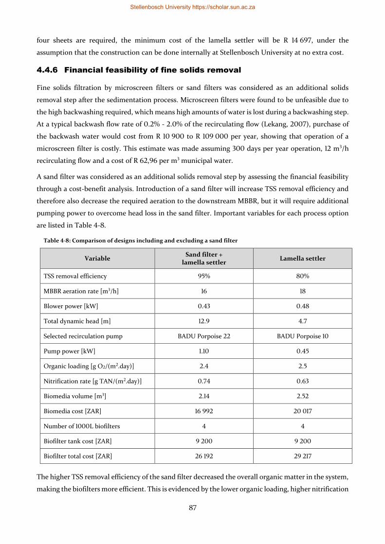
87

four sheets are required, the minimum cost of the lamella settler will be R 14 697, under the

assumption that the construction can be done internally at Stellenbosch University at no extra cost.

4.4.6 Financial feasibility of fine solids removal

Fine solids filtration by microscreen filters or sand filters was considered as an additional solids

removal step after the sedimentation process. Microscreen filters were found to be unfeasible due to

the high backwashing required, which means high amounts of water is lost during a backwashing step.

At a typical backwash flow rate of 0.2% - 2.0% of the recirculating flow (Lekang, 2007), purchase of

the backwash water would cost from R 10 900 to R 109 000 per year, showing that operation of a

microscreen filter is costly. This estimate was made assuming 300 days per year operation, 12 m3/h

recirculating flow and a cost of R 62,96 per m3 municipal water.

A sand filter was considered as an additional solids removal step by assessing the financial feasibility

through a cost-benefit analysis. Introduction of a sand filter will increase TSS removal efficiency and

therefore also decrease the required aeration to the downstream MBBR, but it will require additional

pumping power to overcome head loss in the sand filter. Important variables for each process option

are listed in Table 4-8.

Table 4-8: Comparison of designs including and excluding a sand filter

Variable Sand filter +

lamella settler Lamella settler

TSS removal efficiency 95% 80%

MBBR aeration rate [m3/h] 16 18

Blower power [kW] 0.43 0.48

Total dynamic head [m] 12.9 4.7

Selected recirculation pump BADU Porpoise 22 BADU Porpoise 10

Pump power [kW] 1.10 0.45

Organic loading [g O2/(m2.day)] 2.4 2.5

Nitrification rate [g TAN/(m2.day)] 0.74 0.63

Biomedia volume [m3] 2.14 2.52

Biomedia cost [ZAR] 16 992 20 017

Number of 1000L biofilters 4 4

Biofilter tank cost [ZAR] 9 200 9 200

Biofilter total cost [ZAR] 26 192 29 217

The higher TSS removal efficiency of the sand filter decreased the overall organic matter in the system,

making the biofilters more efficient. This is evidenced by the lower organic loading, higher nitrification


88

rate and lower biomedia volume required to treat the wastewater. The addition of the sand filter

decreased the overall capital cost of the biofilters by approximately R 3 000. The cost of purchasing a

sand filter operating at flow rates of 12 m3/h from online suppliers is R 2699 (Takealot, 2019). The

addition of a sand filter after the lamella settler seemed feasible from purely a capital cost point of

view.

Blower power operating requirements are decreased by 0.05 kW by the addition of a sand filter due

to less organic matter having to be oxidized by heterotrophic bacteria in the biofilter. However, the

pressure drop over the sand filter is estimated to be approximately 80 kPa and thus require specifying

a larger pump. The pump power will be 0.65 kW higher with the addition of a sand filter. The net

power supply required increases by 0.60 kW when adding a sand filter, resulting in an additional

annual operating cost of approximately R 5 900. The savings in capital costs by installing a sand filter

were therefore far outweighed by the significant increases in operating expenditure, and it was

concluded that a sand filter is not a financially feasible addition to the RAS. It should be noted that

backwash water costs associated with periodic backwashing of the sand filter were not included in the

cost benefit analysis due to insufficient information on backwashing frequency, but it is clear from the

analysis that the large increase in electricity costs were enough to deem the sand filter unfeasible.

4.4.7 Conclusion

For the solids removal step in the designed RAS, it was concluded that a lamella settler was the

preferred piece of equipment. A lamella settler was designed to remove coarse suspended particles

and sized by considering various design conditions and performing a sensitivity analysis on the

performance capacity by varying the TSS removal efficiency and the TSS production ratio. Additional

fine solids removal was eliminated by a cost benefit analysis.


89

4.5 Biological filtration design

4.5.1 Evaluation of the existing trickling filters

A previous feeding trial using the existing RAS observed toxic levels of ammonia and nitrite, resulting

in increased water replacement where system water volume was replaced every two weeks (Gericke,

2019). This scenario is undesirable due to the scarcity of freshwater with sufficient water quality in the

area and the high cost of municipal water. The poor performance of the trickling filters in the study

by Gericke (2019) can possibly be attributed to the lack of solids removal resulting in high BOD5 and

thus inhibition of effective nitrification. Another likely cause is the need for trickling filters to be

ventilated properly, ensuring that anaerobic conditions are not present (Eding et al., 2006). The

existing trickling filters are housed in an enclosed chamber and are operated under conditions of zero

forced ventilation, making lack of ventilation a likely cause for the poor nitrification performance.

Therefore, in order to consider the reuse of the existing trickling filters, forced ventilation will need to

be installed.

For the assessment of the existing trickling filters, the trickling filters were assumed to be TAN

diffusion limited and modeled as described in section 3.4.4. When modeling the RAS, the peak daily

TAN production was estimated to be 477 g TAN/day. Nitrification rates are determined by the

hydraulic surface loading rate (HSL) within the model. The minimum required HSL to treat the TAN

produced was estimated to be 381 m3/m2∙day. Given that the total combined cross-sectional area of

the trickling filters is 2.21 m2, a recirculation flow rate of 35 m3/h is required to achieve the required

HSL. The estimated nitrification rates, bulk fluid TAN concentrations and zero-order transition TAN

concentrations (TAN*) within each of the modeled layers of the trickling filters are shown in Figure

4-11. The modeled zero-order transition TAN concentrations were higher than the bulk water TAN

concentrations as seen in Figure 4-11, thereby indicating that the trickling filters would be TAN

diffusion limited throughout. The predicted nitrification rates were adjusted for the effects of

temperature (see section 3.4.8).

The model by Nijhof (1995) used to model the trickling filters did not consider the effect of BOD5 on

the nitrification rate. It is highly probable that lower nitrification rates would be observed in the

existing RAS than the estimated rates (Figure 4-11) due to oxygen diffusion limitation by organic

loading not being taken into account by the trickling filter model. This is supported by comparing the

TAN diffusion limited nitrification rates estimated for the trickling filters (Figure 4-11) with the oxygen

diffusion limited nitrification rates used in the MBBR modeling (see section 3.4.6.2). Applying the

MBBR nitrification rates directly to the trickling filter modeling could be inaccurate since the hydraulic

and aeration operation of the two filters types are vastly different. However, the possibility of lower

nitrification rates than those in Figure 4-11 remains a concern that requires more research.


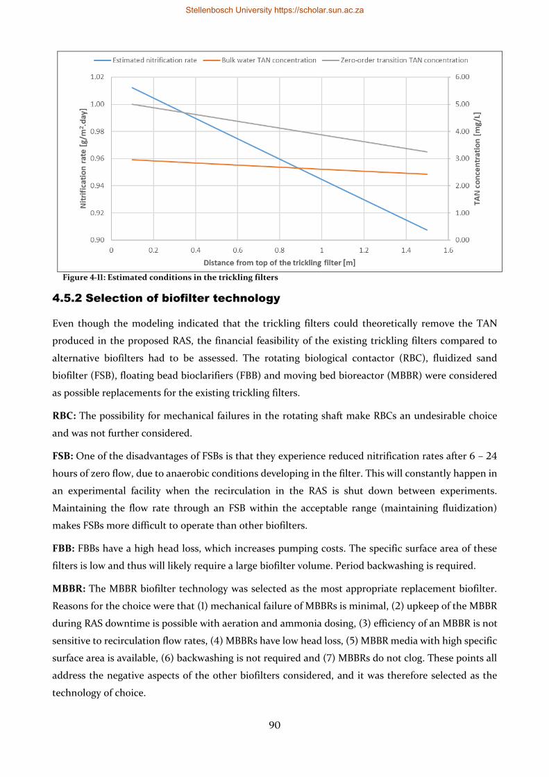
90

Figure 4-11: Estimated conditions in the trickling filters

4.5.2 Selection of biofilter technology

Even though the modeling indicated that the trickling filters could theoretically remove the TAN

produced in the proposed RAS, the financial feasibility of the existing trickling filters compared to

alternative biofilters had to be assessed. The rotating biological contactor (RBC), fluidized sand

biofilter (FSB), floating bead bioclarifiers (FBB) and moving bed bioreactor (MBBR) were considered

as possible replacements for the existing trickling filters.

RBC: The possibility for mechanical failures in the rotating shaft make RBCs an undesirable choice

and was not further considered.

FSB: One of the disadvantages of FSBs is that they experience reduced nitrification rates after 6 – 24

hours of zero flow, due to anaerobic conditions developing in the filter. This will constantly happen in

an experimental facility when the recirculation in the RAS is shut down between experiments.

Maintaining the flow rate through an FSB within the acceptable range (maintaining fluidization)

makes FSBs more difficult to operate than other biofilters.

FBB: FBBs have a high head loss, which increases pumping costs. The specific surface area of these

filters is low and thus will likely require a large biofilter volume. Period backwashing is required.

MBBR: The MBBR biofilter technology was selected as the most appropriate replacement biofilter.

Reasons for the choice were that (1) mechanical failure of MBBRs is minimal, (2) upkeep of the MBBR

during RAS downtime is possible with aeration and ammonia dosing, (3) efficiency of an MBBR is not

sensitive to recirculation flow rates, (4) MBBRs have low head loss, (5) MBBR media with high specific

surface area is available, (6) backwashing is not required and (7) MBBRs do not clog. These points all

address the negative aspects of the other biofilters considered, and it was therefore selected as the

technology of choice.


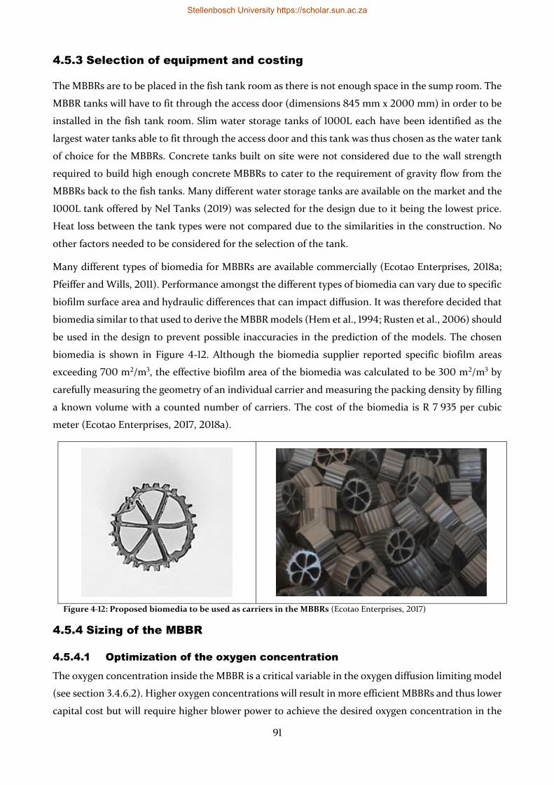
91

4.5.3 Selection of equipment and costing

The MBBRs are to be placed in the fish tank room as there is not enough space in the sump room. The

MBBR tanks will have to fit through the access door (dimensions 845 mm x 2000 mm) in order to be

installed in the fish tank room. Slim water storage tanks of 1000L each have been identified as the

largest water tanks able to fit through the access door and this tank was thus chosen as the water tank

of choice for the MBBRs. Concrete tanks built on site were not considered due to the wall strength

required to build high enough concrete MBBRs to cater to the requirement of gravity flow from the

MBBRs back to the fish tanks. Many different water storage tanks are available on the market and the

1000L tank offered by Nel Tanks (2019) was selected for the design due to it being the lowest price.

Heat loss between the tank types were not compared due to the similarities in the construction. No

other factors needed to be considered for the selection of the tank.

Many different types of biomedia for MBBRs are available commercially (Ecotao Enterprises, 2018a;

Pfeiffer and Wills, 2011). Performance amongst the different types of biomedia can vary due to specific

biofilm surface area and hydraulic differences that can impact diffusion. It was therefore decided that

biomedia similar to that used to derive the MBBR models (Hem et al., 1994; Rusten et al., 2006) should

be used in the design to prevent possible inaccuracies in the prediction of the models. The chosen

biomedia is shown in Figure 4-12. Although the biomedia supplier reported specific biofilm areas

exceeding 700 m2/m3, the effective biofilm area of the biomedia was calculated to be 300 m2/m3 by

carefully measuring the geometry of an individual carrier and measuring the packing density by filling

a known volume with a counted number of carriers. The cost of the biomedia is R 7 935 per cubic

meter (Ecotao Enterprises, 2017, 2018a).

Figure 4-12: Proposed biomedia to be used as carriers in the MBBRs (Ecotao Enterprises, 2017)

4.5.4 Sizing of the MBBR

4.5.4.1 Optimization of the oxygen concentration

The oxygen concentration inside the MBBR is a critical variable in the oxygen diffusion limiting model

(see section 3.4.6.2). Higher oxygen concentrations will result in more efficient MBBRs and thus lower

capital cost but will require higher blower power to achieve the desired oxygen concentration in the


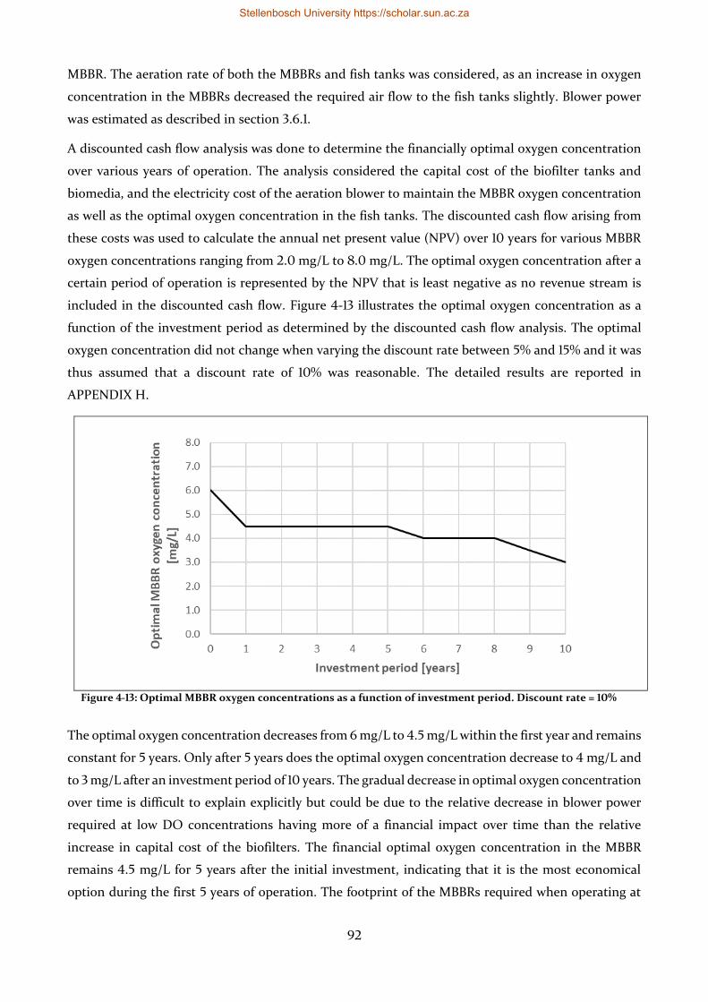
92

MBBR. The aeration rate of both the MBBRs and fish tanks was considered, as an increase in oxygen

concentration in the MBBRs decreased the required air flow to the fish tanks slightly. Blower power

was estimated as described in section 3.6.1.

A discounted cash flow analysis was done to determine the financially optimal oxygen concentration

over various years of operation. The analysis considered the capital cost of the biofilter tanks and

biomedia, and the electricity cost of the aeration blower to maintain the MBBR oxygen concentration

as well as the optimal oxygen concentration in the fish tanks. The discounted cash flow arising from

these costs was used to calculate the annual net present value (NPV) over 10 years for various MBBR

oxygen concentrations ranging from 2.0 mg/L to 8.0 mg/L. The optimal oxygen concentration after a

certain period of operation is represented by the NPV that is least negative as no revenue stream is

included in the discounted cash flow. Figure 4-13 illustrates the optimal oxygen concentration as a

function of the investment period as determined by the discounted cash flow analysis. The optimal

oxygen concentration did not change when varying the discount rate between 5% and 15% and it was

thus assumed that a discount rate of 10% was reasonable. The detailed results are reported in

APPENDIX H.

Figure 4-13: Optimal MBBR oxygen concentrations as a function of investment period. Discount rate = 10%

The optimal oxygen concentration decreases from 6 mg/L to 4.5 mg/L within the first year and remains

constant for 5 years. Only after 5 years does the optimal oxygen concentration decrease to 4 mg/L and

to 3 mg/L after an investment period of 10 years. The gradual decrease in optimal oxygen concentration

over time is difficult to explain explicitly but could be due to the relative decrease in blower power

required at low DO concentrations having more of a financial impact over time than the relative

increase in capital cost of the biofilters. The financial optimal oxygen concentration in the MBBR

remains 4.5 mg/L for 5 years after the initial investment, indicating that it is the most economical

option during the first 5 years of operation. The footprint of the MBBRs required when operating at


93

4.5 mg O2/L was found to fit into the footprint available for the WWT section. Thus, it was decided to

operate the MBBRs at 4.5 mg/L.

4.5.4.2 Initial sizing

Initial MBBR sizing was based on an estimated peak daily TAN production of 477 g TAN/day that is

estimated to be produced on the 91st day of a growth trial at maximum fish stocking density. The peak

daily production of DOM and POM was estimated as 2333 g/day and 1930 g/day respectively. The

POM production was assumed to be equal to the TSS production and thus the effective daily POM

production is reduced by the solids removal steps. Given the TSS removal efficiency of 80%, the POM

production contributing to BOD5 is only 467 g/day at peak loading. Peak daily BOD5 production

reaching the biofilters was estimated to be 1930 g O2/day, where 1407 g O2/day can be attributed to

DOM and 523 g O2/day can be attributed to POM. The percentage filling of the MBBRs with biomedia

was assumed to be 65%.

The models used to model the MBBR (see section 3.4.6) depend on TAN concentration in the MBBR

(TAN diffusion limiting) or oxygen concentration and organic loading (oxygen diffusion limiting). The

model with the lowest nitrification rate prediction was assumed to be the observed nitrification rate.

Decreasing the biofilm area in the MBBR increased the organic loading per biofilm surface area and

thus decreased the nitrification capacity of the MBBR. The MBBR was sized by running a Solver routine

on the model using Microsoft Excel to minimize the biofilm area whilst maintaining the required

nitrification capacity. The results of this initial sizing are given in Table 4-9.

Table 4-9: Initial sizing results for the MBBR design

Variable Value

Organic loading [g O2/(m2.day)] 2.4

Nitrification rate [g TAN/(m2.day)] 0.63

MBBR TAN outlet concentration [mg/L] 0.26

MBBR TAN removal efficiency 91.5%

Biomedia volume [m3] 2.52

Number of 1000L biofilters 4

Combined total residence time of biofilters [min] 32

Required recirculation flow rate [m3/h] 7.3

4.5.4.3 Sensitivity analysis

The sizing described above did not consider the possible variations in the input variables. The effects

on the design when changing the input variables within their ranges observed in literature was

investigated in the sensitivity analysis below in Table 4-10.

The sensitivity analysis showed that the MBBRs need to be oversized for the maximum possible TSS

production ratio case. This is explained by the profound effect of TSS on the organic loading inside

the MBBR. A TSS production ratio of 0.43 g TSS/g dry feed will result in an estimated nitrification rate


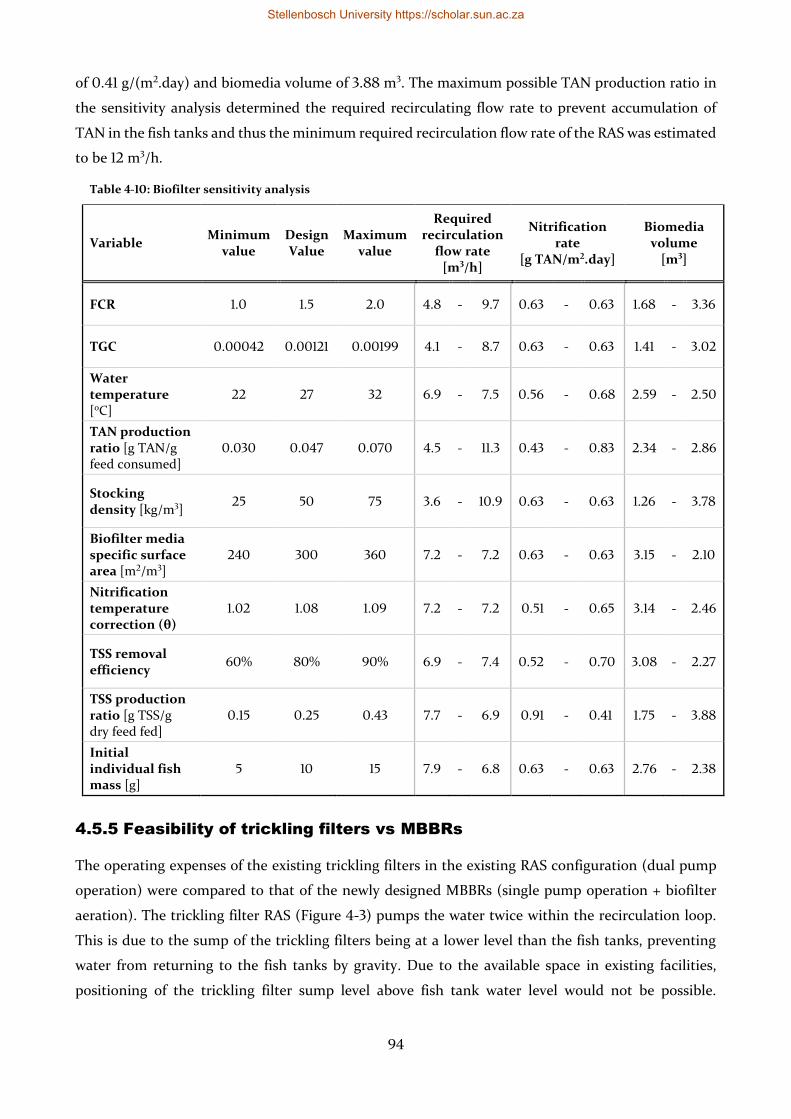
94

of 0.41 g/(m2.day) and biomedia volume of 3.88 m3. The maximum possible TAN production ratio in

the sensitivity analysis determined the required recirculating flow rate to prevent accumulation of

TAN in the fish tanks and thus the minimum required recirculation flow rate of the RAS was estimated

to be 12 m3/h.

Table 4-10: Biofilter sensitivity analysis

Variable Minimum

value Design Value

Maximum value

Required recirculation

flow rate [m3/h]

Nitrification rate

[g TAN/m2.day]

Biomedia volume

[m3]

FCR 1.0 1.5 2.0 4.8 - 9.7 0.63 - 0.63 1.68 - 3.36

TGC 0.00042 0.00121 0.00199 4.1 - 8.7 0.63 - 0.63 1.41 - 3.02

Water temperature [oC]

22 27 32 6.9 - 7.5 0.56 - 0.68 2.59 - 2.50

TAN production ratio [g TAN/g feed consumed]

0.030 0.047 0.070 4.5 - 11.3 0.43 - 0.83 2.34 - 2.86

Stocking density [kg/m3]

25 50 75 3.6 - 10.9 0.63 - 0.63 1.26 - 3.78

Biofilter media specific surface area [m2/m3]

240 300 360 7.2 - 7.2 0.63 - 0.63 3.15 - 2.10

Nitrification temperature correction (θ)

1.02 1.08 1.09 7.2 - 7.2 0.51 - 0.65 3.14 - 2.46

TSS removal efficiency

60% 80% 90% 6.9 - 7.4 0.52 - 0.70 3.08 - 2.27

TSS production ratio [g TSS/g dry feed fed]

0.15 0.25 0.43 7.7 - 6.9 0.91 - 0.41 1.75 - 3.88

Initial individual fish mass [g]

5 10 15 7.9 - 6.8 0.63 - 0.63 2.76 - 2.38

4.5.5 Feasibility of trickling filters vs MBBRs

The operating expenses of the existing trickling filters in the existing RAS configuration (dual pump

operation) were compared to that of the newly designed MBBRs (single pump operation + biofilter

aeration). The trickling filter RAS (Figure 4-3) pumps the water twice within the recirculation loop.

This is due to the sump of the trickling filters being at a lower level than the fish tanks, preventing

water from returning to the fish tanks by gravity. Due to the available space in existing facilities,

positioning of the trickling filter sump level above fish tank water level would not be possible.


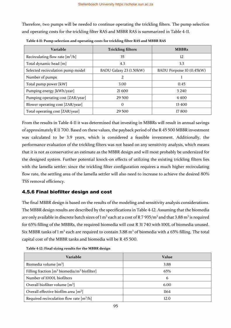
95

Therefore, two pumps will be needed to continue operating the trickling filters. The pump selection

and operating costs for the trickling filter RAS and MBBR RAS is summarized in Table 4-11.

Table 4-11: Pump selection and operating costs for trickling filter RAS and MBBR RAS

Variable Trickling filters MBBRs

Recirculating flow rate [m3/h] 35 12

Total dynamic head [m] 4.3 3.3

Selected recirculation pump model BADU Galaxy 23 (1.50kW) BADU Porpoise 10 (0.45kW)

Number of pumps 2 1

Total pump power [kW] 3.00 0.45

Pumping energy [kWh/year] 21 600 3 240

Pumping operating cost [ZAR/year] 29 500 4 400

Blower operating cost [ZAR/year] 0 13 400

Total operating cost [ZAR/year] 29 500 17 800

From the results in Table 4-11 it was determined that investing in MBBRs will result in annual savings

of approximately R 11 700. Based on these values, the payback period of the R 45 500 MBBR investment

was calculated to be 3.9 years, which is considered a feasible investment. Additionally, the

performance evaluation of the trickling filters was not based on any sensitivity analysis, which means

that it is not as conservative an estimate as the MBBR design and will most probably be undersized for

the designed system. Further potential knock-on effects of utilizing the existing trickling filters lies

with the lamella settler: since the trickling filter configuration requires a much higher recirculating

flow rate, the settling area of the lamella settler will also need to increase to achieve the desired 80%

TSS removal efficiency.

4.5.6 Final biofilter design and cost

The final MBBR design is based on the results of the modeling and sensitivity analysis considerations.

The MBBR design results are described by the specifications in Table 4-12. Assuming that the biomedia

are only available in discrete batch sizes of 1 m3 each at a cost of R 7 935/m3 and that 3.88 m3 is required

for 65% filling of the MBBRs, the required biomedia will cost R 31 740 with 100L of biomedia unused.

Six MBBR tanks of 1 m3 each are required to contain 3.88 m3 of biomedia with a 65% filling. The total

capital cost of the MBBR tanks and biomedia will be R 45 500.

Table 4-12: Final sizing results for the MBBR design

Variable Value

Biomedia volume [m3] 3.88

Filling fraction [m3 biomedia/m3 biofilter] 65%

Number of 1000L biofilters 6

Overall biofilter volume [m3] 6.00

Overall effective biofilm area [m2] 1164

Required recirculation flow rate [m3/h] 12.0


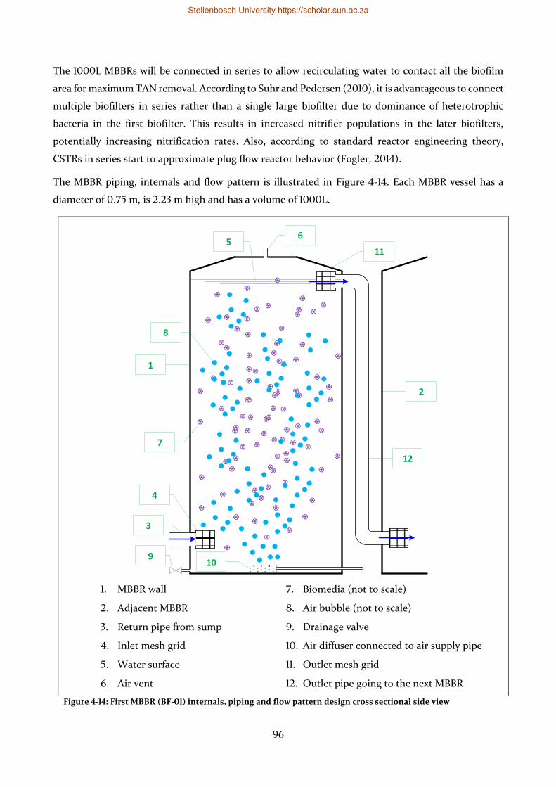
96

The 1000L MBBRs will be connected in series to allow recirculating water to contact all the biofilm

area for maximum TAN removal. According to Suhr and Pedersen (2010), it is advantageous to connect

multiple biofilters in series rather than a single large biofilter due to dominance of heterotrophic

bacteria in the first biofilter. This results in increased nitrifier populations in the later biofilters,

potentially increasing nitrification rates. Also, according to standard reactor engineering theory,

CSTRs in series start to approximate plug flow reactor behavior (Fogler, 2014).

The MBBR piping, internals and flow pattern is illustrated in Figure 4-14. Each MBBR vessel has a

diameter of 0.75 m, is 2.23 m high and has a volume of 1000L.

1. MBBR wall

2. Adjacent MBBR

3. Return pipe from sump

4. Inlet mesh grid

5. Water surface

6. Air vent

7. Biomedia (not to scale)

8. Air bubble (not to scale)

9. Drainage valve

10. Air diffuser connected to air supply pipe

11. Outlet mesh grid

12. Outlet pipe going to the next MBBR

Figure 4-14: First MBBR (BF-01) internals, piping and flow pattern design cross sectional side view

1

2

56

7

8

4

910

11

12

3


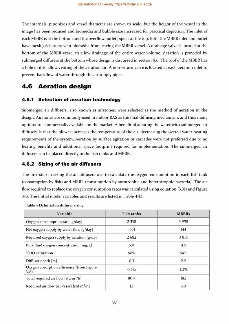
97

The internals, pipe sizes and vessel diameter are shown to scale, but the height of the vessel in the

image has been reduced and biomedia and bubble size increased for practical depiction. The inlet of

each MBBR is at the bottom and the overflow outlet pipe is at the top. Both the MBBR inlet and outlet

have mesh grids to prevent biomedia from leaving the MBBR vessel. A drainage valve is located at the

bottom of the MBBR vessel to allow drainage of the entire water volume. Aeration is provided by

submerged diffusers at the bottom whose design is discussed in section 4.6. The roof of the MBBR has

a hole in it to allow venting of the aeration air. A non-return valve is located at each aeration inlet to

prevent backflow of water through the air supply pipes.

4.6 Aeration design

4.6.1 Selection of aeration technology

Submerged air diffusers, also known as airstones, were selected as the method of aeration in the

design. Airstones are commonly used in indoor RAS as the final diffusing mechanism, and thus many

options are commercially available on the market. A benefit of aerating the water with submerged air

diffusers is that the blower increases the temperature of the air, decreasing the overall water heating

requirements of the system. Aeration by surface agitation or cascades were not preferred due to no

heating benefits and additional space footprint required for implementation. The submerged air

diffusers can be placed directly in the fish tanks and MBBR.

4.6.2 Sizing of the air diffusers

The first step in sizing the air diffusers was to calculate the oxygen consumption in each fish tank

(consumption by fish) and MBBR (consumption by autotrophic and heterotrophic bacteria). The air

flow required to replace the oxygen consumption rates was calculated using equation (3.31) and Figure

3-8. The initial model variables and results are listed in Table 4-13.

Table 4-13: Initial air diffuser sizing

Variable Fish tanks MBBRs

Oxygen consumption rate [g/day] 2 538 3 958

Net oxygen supply by water flow [g/day] -144 144

Required oxygen supply by aeration [g/day] 2 682 3 814

Bulk fluid oxygen concentration [mg/L] 5.0 4.5

%DO saturation 60% 54%

Diffuser depth [m] 0.3 2.2

Oxygen absorption efficiency (from Figure 3-8)

0.5% 3.2%

Total required air flow [std m3/h] 80.7 18.1

Required air flow per vessel [std m3/h] 1.1 3.0


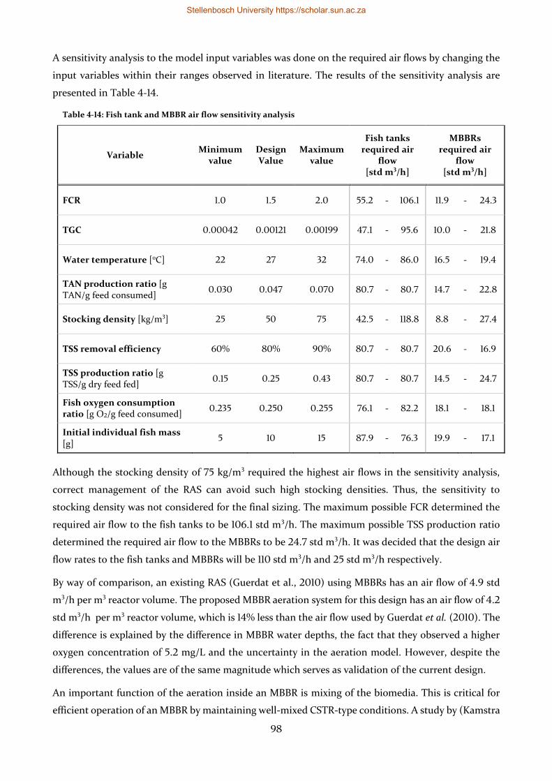
98

A sensitivity analysis to the model input variables was done on the required air flows by changing the

input variables within their ranges observed in literature. The results of the sensitivity analysis are

presented in Table 4-14.

Table 4-14: Fish tank and MBBR air flow sensitivity analysis

Variable Minimum

value Design Value

Maximum value

Fish tanks required air

flow [std m3/h]

MBBRs required air

flow [std m3/h]

FCR 1.0 1.5 2.0 55.2 - 106.1 11.9 - 24.3

TGC 0.00042 0.00121 0.00199 47.1 - 95.6 10.0 - 21.8

Water temperature [oC] 22 27 32 74.0 - 86.0 16.5 - 19.4

TAN production ratio [g TAN/g feed consumed]

0.030 0.047 0.070 80.7 - 80.7 14.7 - 22.8

Stocking density [kg/m3] 25 50 75 42.5 - 118.8 8.8 - 27.4

TSS removal efficiency 60% 80% 90% 80.7 - 80.7 20.6 - 16.9

TSS production ratio [g TSS/g dry feed fed]

0.15 0.25 0.43 80.7 - 80.7 14.5 - 24.7

Fish oxygen consumption ratio [g O2/g feed consumed]

0.235 0.250 0.255 76.1 - 82.2 18.1 - 18.1

Initial individual fish mass [g]

5 10 15 87.9 - 76.3 19.9 - 17.1

Although the stocking density of 75 kg/m3 required the highest air flows in the sensitivity analysis,

correct management of the RAS can avoid such high stocking densities. Thus, the sensitivity to

stocking density was not considered for the final sizing. The maximum possible FCR determined the

required air flow to the fish tanks to be 106.1 std m3/h. The maximum possible TSS production ratio

determined the required air flow to the MBBRs to be 24.7 std m3/h. It was decided that the design air

flow rates to the fish tanks and MBBRs will be 110 std m3/h and 25 std m3/h respectively.

By way of comparison, an existing RAS (Guerdat et al., 2010) using MBBRs has an air flow of 4.9 std

m3/h per m3 reactor volume. The proposed MBBR aeration system for this design has an air flow of 4.2

std m3/h per m3 reactor volume, which is 14% less than the air flow used by Guerdat et al. (2010). The

difference is explained by the difference in MBBR water depths, the fact that they observed a higher

oxygen concentration of 5.2 mg/L and the uncertainty in the aeration model. However, despite the

differences, the values are of the same magnitude which serves as validation of the current design.

An important function of the aeration inside an MBBR is mixing of the biomedia. This is critical for

efficient operation of an MBBR by maintaining well-mixed CSTR-type conditions. A study by (Kamstra


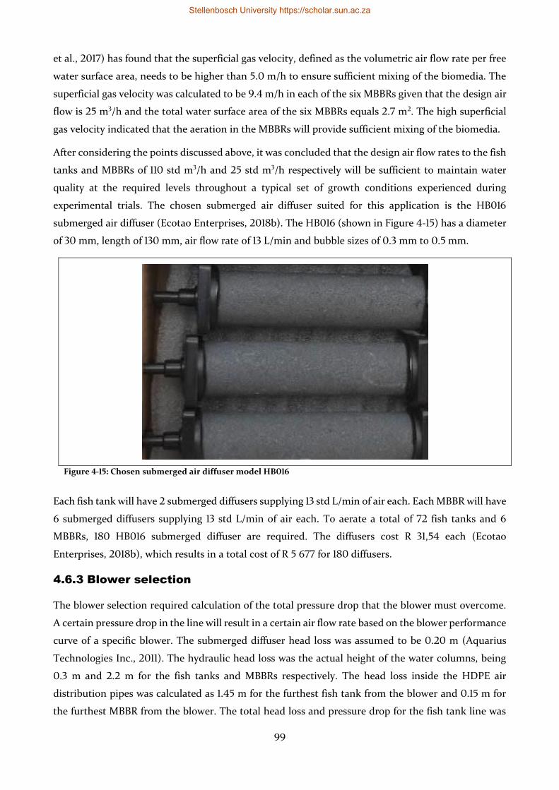
99

et al., 2017) has found that the superficial gas velocity, defined as the volumetric air flow rate per free

water surface area, needs to be higher than 5.0 m/h to ensure sufficient mixing of the biomedia. The

superficial gas velocity was calculated to be 9.4 m/h in each of the six MBBRs given that the design air

flow is 25 m3/h and the total water surface area of the six MBBRs equals 2.7 m2. The high superficial

gas velocity indicated that the aeration in the MBBRs will provide sufficient mixing of the biomedia.

After considering the points discussed above, it was concluded that the design air flow rates to the fish

tanks and MBBRs of 110 std m3/h and 25 std m3/h respectively will be sufficient to maintain water

quality at the required levels throughout a typical set of growth conditions experienced during

experimental trials. The chosen submerged air diffuser suited for this application is the HB016

submerged air diffuser (Ecotao Enterprises, 2018b). The HB016 (shown in Figure 4-15) has a diameter

of 30 mm, length of 130 mm, air flow rate of 13 L/min and bubble sizes of 0.3 mm to 0.5 mm.

Figure 4-15: Chosen submerged air diffuser model HB016

Each fish tank will have 2 submerged diffusers supplying 13 std L/min of air each. Each MBBR will have

6 submerged diffusers supplying 13 std L/min of air each. To aerate a total of 72 fish tanks and 6

MBBRs, 180 HB016 submerged diffuser are required. The diffusers cost R 31,54 each (Ecotao

Enterprises, 2018b), which results in a total cost of R 5 677 for 180 diffusers.

4.6.3 Blower selection

The blower selection required calculation of the total pressure drop that the blower must overcome.

A certain pressure drop in the line will result in a certain air flow rate based on the blower performance

curve of a specific blower. The submerged diffuser head loss was assumed to be 0.20 m (Aquarius

Technologies Inc., 2011). The hydraulic head loss was the actual height of the water columns, being

0.3 m and 2.2 m for the fish tanks and MBBRs respectively. The head loss inside the HDPE air

distribution pipes was calculated as 1.45 m for the furthest fish tank from the blower and 0.15 m for

the furthest MBBR from the blower. The total head loss and pressure drop for the fish tank line was


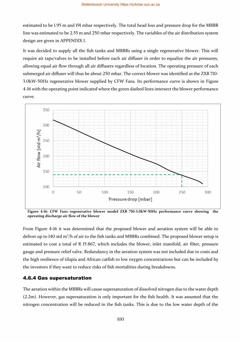
100

estimated to be 1.95 m and 191 mbar respectively. The total head loss and pressure drop for the MBBR

line was estimated to be 2.55 m and 250 mbar respectively. The variables of the air distribution system

design are given in APPENDIX I.

It was decided to supply all the fish tanks and MBBRs using a single regenerative blower. This will

require air taps/valves to be installed before each air diffuser in order to equalize the air pressures,

allowing equal air flow through all air diffusers regardless of location. The operating pressure of each

submerged air diffuser will thus be about 250 mbar. The correct blower was identified as the ZXB 710-

3.0kW-50Hz regenerative blower supplied by CFW Fans. Its performance curve is shown in Figure

4-16 with the operating point indicated where the green dashed lines intersect the blower performance

curve.

Figure 4-16: CFW Fans regenerative blower model ZXB 710-3.0kW-50Hz performance curve showing the operating discharge air flow of the blower

From Figure 4-16 it was determined that the proposed blower and aeration system will be able to

deliver up to 140 std m3/h of air to the fish tanks and MBBRs combined. The proposed blower setup is

estimated to cost a total of R 15 867, which includes the blower, inlet manifold, air filter, pressure

gauge and pressure relief valve. Redundancy in the aeration system was not included due to costs and

the high resilience of tilapia and African catfish to low oxygen concentrations but can be included by

the investors if they want to reduce risks of fish mortalities during breakdowns.

4.6.4 Gas supersaturation

The aeration within the MBBRs will cause supersaturation of dissolved nitrogen due to the water depth

(2.2m). However, gas supersaturation is only important for the fish health. It was assumed that the

nitrogen concentration will be reduced in the fish tanks. This is due to the low water depth of the


101

tanks causing lower nitrogen saturation concentrations and the vigorous aeration in the fish tanks

causing equilibrium conditions for dissolved nitrogen.

The 𝜑-value for fine bubble diffusers was used for nitrogen saturation concentration correction using

equation (3.30) as fine bubble diffusers will account the most of the supersaturation. The results of

the gas supersaturation evaluation in the fish tanks are given in Table 4-15.

Table 4-15: Gas supersaturation results

Variable Value Units

Effective nitrogen saturation concentration 14.1 𝑚𝑔 𝐿⁄

Nitrogen gas tension 611 𝑚𝑚𝐻𝑔

Local barometric pressure (BP) 760 𝑚𝑚𝐻𝑔

Case 1: Normal operation, fish tank DO concentration = 5.0 𝑚𝑔 𝐿⁄

Oxygen gas tension 97 𝑚𝑚𝐻𝑔

Total dissolved gas pressure (TGP) 708 𝑚𝑚𝐻𝑔

DP (TGP – BP) -52 𝑚𝑚𝐻𝑔

%TGP 93%

Case 2: 100% oxygen saturation, fish tank DO concentration = 8.8 𝑚𝑔 𝐿⁄

Oxygen gas tension 170 𝑚𝑚𝐻𝑔

Total dissolved gas pressure (TGP) 781 𝑚𝑚𝐻𝑔

DP (TGP – BP) 21 𝑚𝑚𝐻𝑔

%TGP 103%

The two cases considered in Table 4-15 were the design oxygen concentration of 5 mg/L and a worst-

case scenario of the fish tank water being saturated with oxygen to determine if there is any risk of gas

supersaturation in the fish tanks. The water is not supersaturated with gas at case 1 because DP < 0.

Thus, no risk of gas bubble disease is present in case 1. It was found that the water is supersaturated

with gas in case 2 due to DP > 0. However, the DP exceeds the recommended limit of 20 mmHg by

only 1 mmHg. The %TGP is below the literature limit of 106%. Case 2 is extremely unlikely due to

constant consumption of oxygen by the fish and the fact that air is used for oxygenation instead of

pure oxygen. Air flow rates required to achieve near 100% oxygen saturation is exceptionally high in

the presence of intensive fish culture (Timmons and Ebeling, 2007). In conclusion, there is no risk of

gas bubble disease in the proposed system.

4.6.5 Carbon dioxide degassing

At the estimated oxygen consumption rate in the fish tanks of 2538 g O2/day, the carbon dioxide

production rate was estimated to be 3490 g CO2/day by considering the stoichiometry of the

respiration (see section 3.3.2). 𝐾𝐿𝑎𝑂2 was calculated to be 130 day-1 and using the ratio of

𝐾𝐿𝑎𝐶𝑂2

𝐾𝐿𝑎𝑂2

= 0.9,

𝐾𝐿𝑎𝐶𝑂2 was calculated to be 117 day-1. To find the steady state carbon dioxide concentration in the fish

tanks, a carbon dioxide mass balance was done over the fish tanks. The effect of water inflow and

outflow was assumed to be negligible. The removal of carbon dioxide by degassing and production of

carbon dioxide by fish respiration were the only flows of carbon dioxide considered in the mass

balance. Thereby steady state will be reached when the removal rate is equal to the production rate.


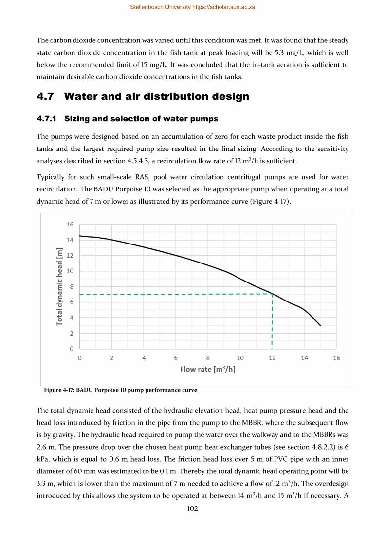
102

The carbon dioxide concentration was varied until this condition was met. It was found that the steady

state carbon dioxide concentration in the fish tank at peak loading will be 5.3 mg/L, which is well

below the recommended limit of 15 mg/L. It was concluded that the in-tank aeration is sufficient to

maintain desirable carbon dioxide concentrations in the fish tanks.

4.7 Water and air distribution design

4.7.1 Sizing and selection of water pumps

The pumps were designed based on an accumulation of zero for each waste product inside the fish

tanks and the largest required pump size resulted in the final sizing. According to the sensitivity

analyses described in section 4.5.4.3, a recirculation flow rate of 12 m3/h is sufficient.

Typically for such small-scale RAS, pool water circulation centrifugal pumps are used for water

recirculation. The BADU Porpoise 10 was selected as the appropriate pump when operating at a total

dynamic head of 7 m or lower as illustrated by its performance curve (Figure 4-17).

Figure 4-17: BADU Porpoise 10 pump performance curve

The total dynamic head consisted of the hydraulic elevation head, heat pump pressure head and the

head loss introduced by friction in the pipe from the pump to the MBBR, where the subsequent flow

is by gravity. The hydraulic head required to pump the water over the walkway and to the MBBRs was

2.6 m. The pressure drop over the chosen heat pump heat exchanger tubes (see section 4.8.2.2) is 6

kPa, which is equal to 0.6 m head loss. The friction head loss over 5 m of PVC pipe with an inner

diameter of 60 mm was estimated to be 0.1 m. Thereby the total dynamic head operating point will be

3.3 m, which is lower than the maximum of 7 m needed to achieve a flow of 12 m3/h. The overdesign

introduced by this allows the system to be operated at between 14 m3/h and 15 m3/h if necessary. A


103

valve and flow meter will need to be installed at the pump to manually control the recirculating flow

at 12 m3/h as high flows can decrease the efficiency of the lamella settler.

A backup pump is required in case of pump failure or maintenance as the build-up of ammonia and

solids inside the fish tanks could be fatal to the fish and needs to be transported to the solids removal

and biofiltration unit operations. The current existing system does have two BADU Porpoise 10 pumps

and thus no new pumps have to be purchased.

4.7.2 Water and air piping design

The chosen water pipes were uPVC piping, which is the standard pipe material used for RAS in South

Africa. The chosen air pipes were HDPE piping. Both the water and air pipe diameters were chosen to

minimize head loss and not allowing water velocities faster than 2.5 m/s. Higher water velocities in

pipes can cause noise and damage to pipes if flow stops suddenly. The complete water and air

distribution design is described by the piping and instrumentation diagrams (P&IDs) in APPENDIX

C. The general layout of the water and air piping is shown in Figure 4-18.


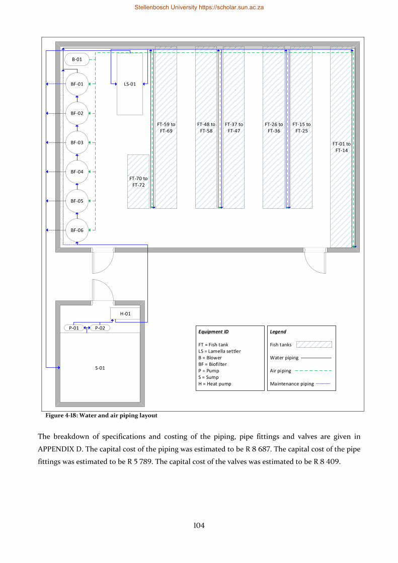
104

Figure 4-18: Water and air piping layout

The breakdown of specifications and costing of the piping, pipe fittings and valves are given in

APPENDIX D. The capital cost of the piping was estimated to be R 8 687. The capital cost of the pipe

fittings was estimated to be R 5 789. The capital cost of the valves was estimated to be R 8 409.

FT-26 to FT-36

FT-01 to FT-14

FT-15 to FT-25

FT-48 to FT-58

FT-37 to FT-47

FT-70 to FT-72

FT-59 to FT-69

BF-06

BF-05

BF-04

BF-03

BF-02

BF-01 LS-01

S-01

P-01 P-02

H-01

Legend

Fish tanks

Water piping

Air piping

Maintenance piping

Equipment ID

FT = Fish tankLS = Lamella settlerB = BlowerBF = BiofilterP = PumpS = SumpH = Heat pump


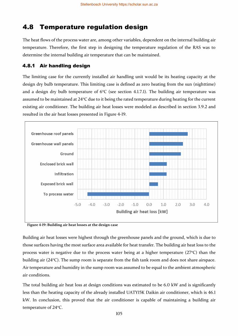
105

4.8 Temperature regulation design

The heat flows of the process water are, among other variables, dependent on the internal building air

temperature. Therefore, the first step in designing the temperature regulation of the RAS was to

determine the internal building air temperature that can be maintained.

4.8.1 Air handling design

The limiting case for the currently installed air handling unit would be its heating capacity at the

design dry bulb temperature. This limiting case is defined as zero heating from the sun (nighttime)

and a design dry bulb temperature of 6oC (see section 4.1.7.1). The building air temperature was

assumed to be maintained at 24oC due to it being the rated temperature during heating for the current

existing air conditioner. The building air heat losses were modeled as described in section 3.9.2 and

resulted in the air heat losses presented in Figure 4-19.

Figure 4-19: Building air heat losses at the design case

Building air heat losses were highest through the greenhouse panels and the ground, which is due to

those surfaces having the most surface area available for heat transfer. The building air heat loss to the

process water is negative due to the process water being at a higher temperature (27oC) than the

building air (24oC). The sump room is separate from the fish tank room and does not share airspace.

Air temperature and humidity in the sump room was assumed to be equal to the ambient atmospheric

air conditions.

The total building air heat loss at design conditions was estimated to be 6.0 kW and is significantly

less than the heating capacity of the already installed UATY15K Daikin air conditioner, which is 46.1

kW. In conclusion, this proved that the air conditioner is capable of maintaining a building air

temperature of 24oC.


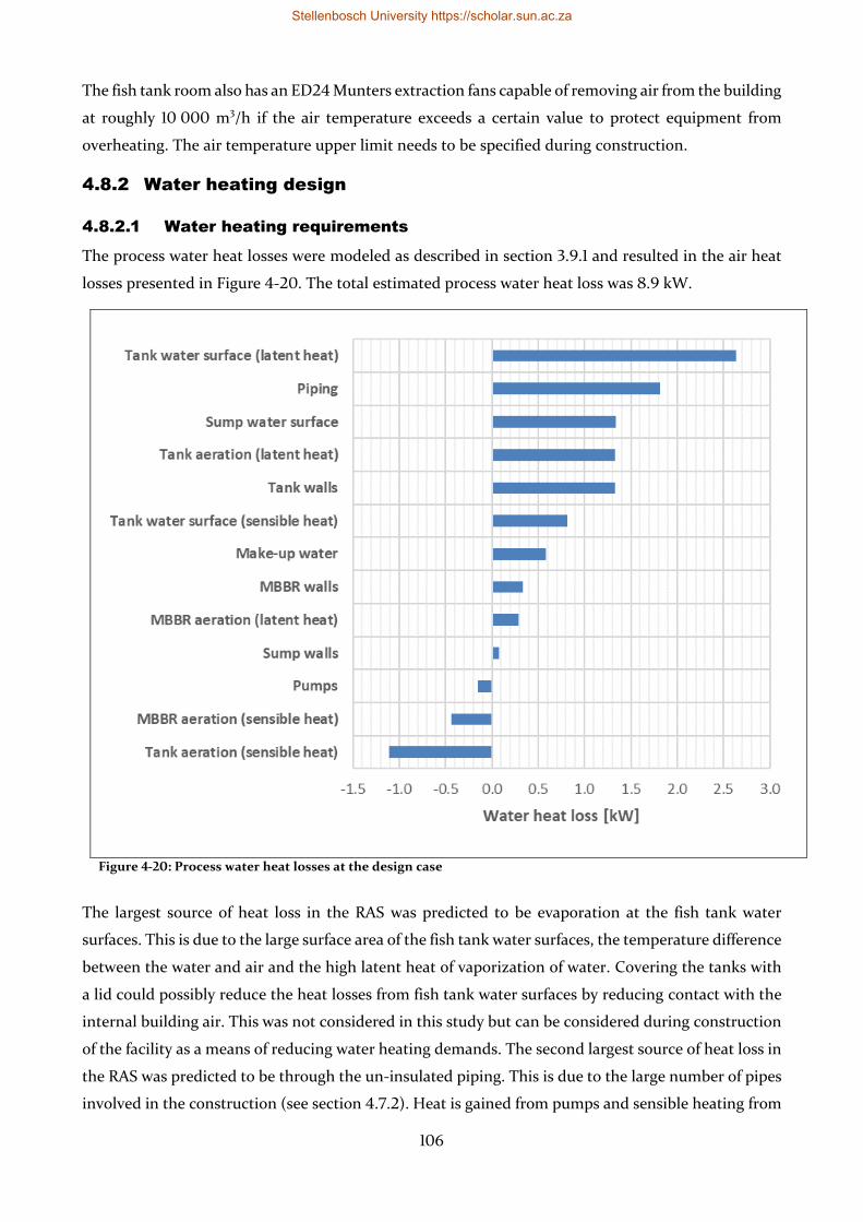
106

The fish tank room also has an ED24 Munters extraction fans capable of removing air from the building

at roughly 10 000 m3/h if the air temperature exceeds a certain value to protect equipment from

overheating. The air temperature upper limit needs to be specified during construction.

4.8.2 Water heating design

4.8.2.1 Water heating requirements

The process water heat losses were modeled as described in section 3.9.1 and resulted in the air heat

losses presented in Figure 4-20. The total estimated process water heat loss was 8.9 kW.

Figure 4-20: Process water heat losses at the design case

The largest source of heat loss in the RAS was predicted to be evaporation at the fish tank water

surfaces. This is due to the large surface area of the fish tank water surfaces, the temperature difference

between the water and air and the high latent heat of vaporization of water. Covering the tanks with

a lid could possibly reduce the heat losses from fish tank water surfaces by reducing contact with the

internal building air. This was not considered in this study but can be considered during construction

of the facility as a means of reducing water heating demands. The second largest source of heat loss in

the RAS was predicted to be through the un-insulated piping. This is due to the large number of pipes

involved in the construction (see section 4.7.2). Heat is gained from pumps and sensible heating from


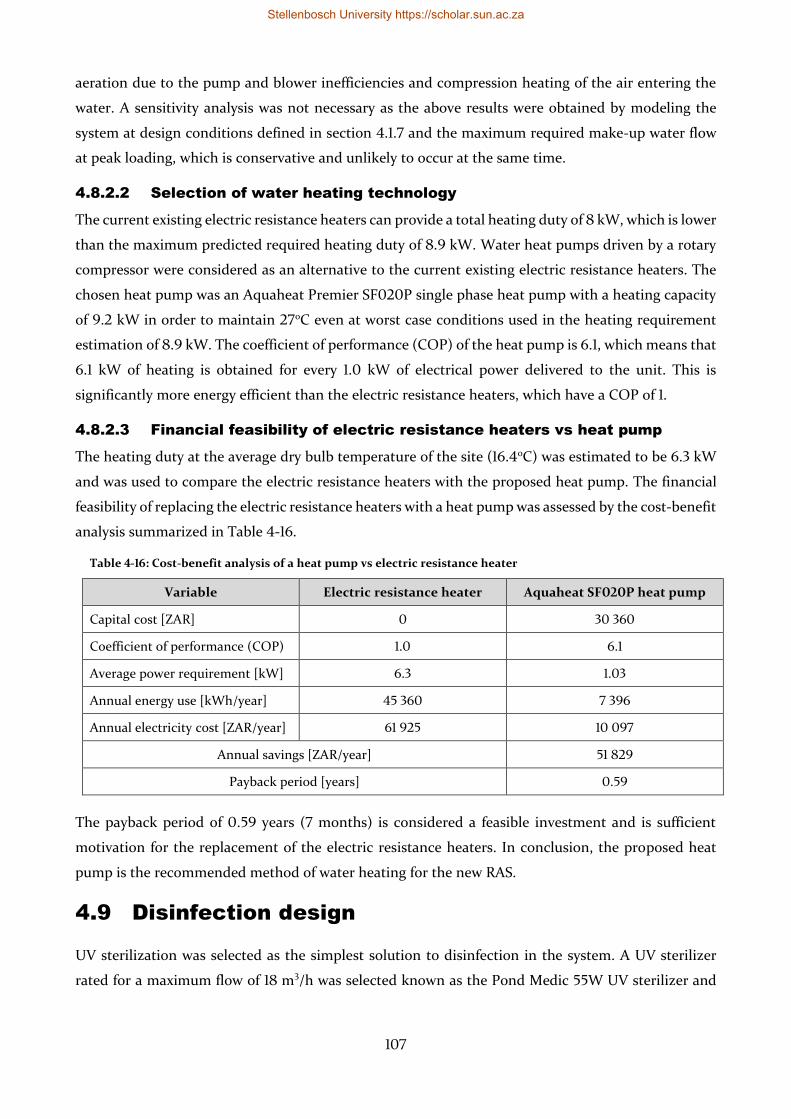
107

aeration due to the pump and blower inefficiencies and compression heating of the air entering the

water. A sensitivity analysis was not necessary as the above results were obtained by modeling the

system at design conditions defined in section 4.1.7 and the maximum required make-up water flow

at peak loading, which is conservative and unlikely to occur at the same time.

4.8.2.2 Selection of water heating technology

The current existing electric resistance heaters can provide a total heating duty of 8 kW, which is lower

than the maximum predicted required heating duty of 8.9 kW. Water heat pumps driven by a rotary

compressor were considered as an alternative to the current existing electric resistance heaters. The

chosen heat pump was an Aquaheat Premier SF020P single phase heat pump with a heating capacity

of 9.2 kW in order to maintain 27oC even at worst case conditions used in the heating requirement

estimation of 8.9 kW. The coefficient of performance (COP) of the heat pump is 6.1, which means that

6.1 kW of heating is obtained for every 1.0 kW of electrical power delivered to the unit. This is

significantly more energy efficient than the electric resistance heaters, which have a COP of 1.

4.8.2.3 Financial feasibility of electric resistance heaters vs heat pump

The heating duty at the average dry bulb temperature of the site (16.4oC) was estimated to be 6.3 kW

and was used to compare the electric resistance heaters with the proposed heat pump. The financial

feasibility of replacing the electric resistance heaters with a heat pump was assessed by the cost-benefit

analysis summarized in Table 4-16.

Table 4-16: Cost-benefit analysis of a heat pump vs electric resistance heater

Variable Electric resistance heater Aquaheat SF020P heat pump

Capital cost [ZAR] 0 30 360

Coefficient of performance (COP) 1.0 6.1

Average power requirement [kW] 6.3 1.03

Annual energy use [kWh/year] 45 360 7 396

Annual electricity cost [ZAR/year] 61 925 10 097

Annual savings [ZAR/year] 51 829

Payback period [years] 0.59

The payback period of 0.59 years (7 months) is considered a feasible investment and is sufficient

motivation for the replacement of the electric resistance heaters. In conclusion, the proposed heat

pump is the recommended method of water heating for the new RAS.

4.9 Disinfection design

UV sterilization was selected as the simplest solution to disinfection in the system. A UV sterilizer

rated for a maximum flow of 18 m3/h was selected known as the Pond Medic 55W UV sterilizer and


108

will cost R 1 099 (Futurama, 2019). The UV sterilizer will be installed in-line at the sump room after

the pump discharge.

4.10 Water quality measurements

For regular monitoring of water quality, the critical water quality parameters must be measured

namely, DO, pH, ammonia, nitrite, nitrate and CO2. Due to the effort required to measure suspended

solids, TSS only needs to be measured if water quality issues arise as part of the troubleshooting

process (see section 5.4.10). Dissolved oxygen concentration measurements can be done manually

using an IP67 DO meter that will cost R 3 750 (MyAquaponics, 2019a). pH and temperature

measurements can be done manually using a pH and temperature meter that will cost R 1 695

(MyAquaponics, 2019b). Online measurement of ammonia, nitrite and nitrate is expensive and

therefore daily manual measurement of these concentrations using low-cost spectrophotometric

methods is required to ensure optimal operations. The costs of these manual measurement methods

were excluded from the cost estimate for the project as the necessary equipment already exists at the

present facility. Carbon dioxide concentrations can be inferred by the pH and total alkalinity.


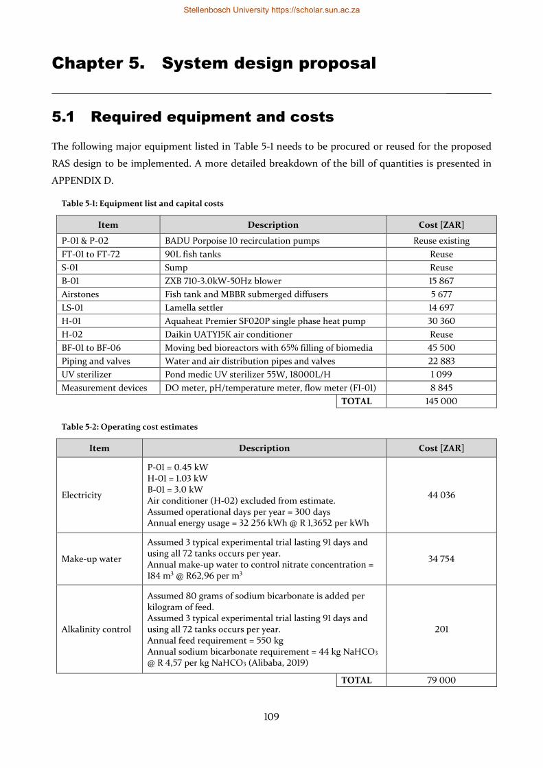
109

Chapter 5. System design proposal

_________

5.1 Required equipment and costs

The following major equipment listed in Table 5-1 needs to be procured or reused for the proposed

RAS design to be implemented. A more detailed breakdown of the bill of quantities is presented in

APPENDIX D.

Table 5-1: Equipment list and capital costs

Item Description Cost [ZAR]

P-01 & P-02 BADU Porpoise 10 recirculation pumps Reuse existing

FT-01 to FT-72 90L fish tanks Reuse

S-01 Sump Reuse

B-01 ZXB 710-3.0kW-50Hz blower 15 867

Airstones Fish tank and MBBR submerged diffusers 5 677

LS-01 Lamella settler 14 697

H-01 Aquaheat Premier SF020P single phase heat pump 30 360

H-02 Daikin UATY15K air conditioner Reuse

BF-01 to BF-06 Moving bed bioreactors with 65% filling of biomedia 45 500

Piping and valves Water and air distribution pipes and valves 22 883

UV sterilizer Pond medic UV sterilizer 55W, 18000L/H 1 099

Measurement devices DO meter, pH/temperature meter, flow meter (FI-01) 8 845

TOTAL 145 000

Table 5-2: Operating cost estimates

Item Description Cost [ZAR]

Electricity

P-01 = 0.45 kW H-01 = 1.03 kW B-01 = 3.0 kW Air conditioner (H-02) excluded from estimate. Assumed operational days per year = 300 days Annual energy usage = 32 256 kWh @ R 1,3652 per kWh

44 036

Make-up water

Assumed 3 typical experimental trial lasting 91 days and using all 72 tanks occurs per year. Annual make-up water to control nitrate concentration = 184 m3 @ R62,96 per m3

34 754

Alkalinity control

Assumed 80 grams of sodium bicarbonate is added per kilogram of feed. Assumed 3 typical experimental trial lasting 91 days and using all 72 tanks occurs per year. Annual feed requirement = 550 kg Annual sodium bicarbonate requirement = 44 kg NaHCO3 @ R 4,57 per kg NaHCO3 (Alibaba, 2019)

201

TOTAL 79 000


110

The estimated capital cost of implementing the proposed RAS design is R 145 000.

Based on the operating estimates described in Table 5-2, the total annual operating cost of the

proposed RAS will be R 79 000. It should noted that the estimated annual operating cost of the RAS

is more than 50% the total estimated capital cost, which further highlights the importance of

considering operating costs versus capital costs of RAS equipment to achieve a financially optimal

design.


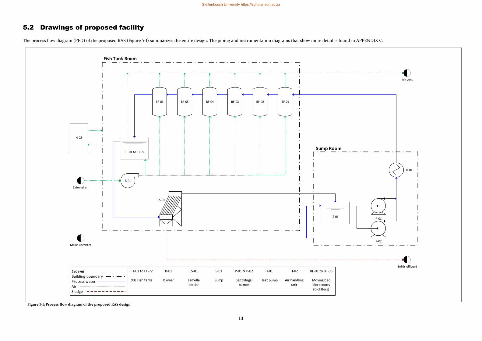
111

5.2 Drawings of proposed facility

The process flow diagram (PFD) of the proposed RAS (Figure 5-1) summarizes the entire design. The piping and instrumentation diagrams that show more detail is found in APPENDIX C.

Figure 5-1: Process flow diagram of the proposed RAS design

Make-up water

H-01

FT-01 to FT-72

90L Fish tanks

P-01 & P-02

Centrifugal pumps

LS-01

Lamella settler

B-01

Blower

S-01

Sump

H-01

Heat pump

H-02

Air handling unit

FT-01 to FT-72

BF-06 BF-05 BF-04 BF-03 BF-02 BF-01

B-01

LS-01

S-01P-01

H-02

Air vent

Fish Tank Room

Sump Room

LegendBuilding boundaryProcess waterAirSludge

Solids effluent

External air

BF-01 to BF-06

Moving bed bioreactors (biofilters)

P-02


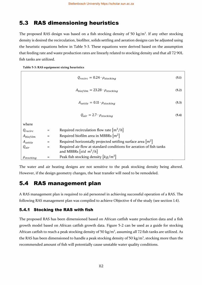
112

5.3 RAS dimensioning heuristics

The proposed RAS design was based on a fish stocking density of 50 kg/m3. If any other stocking

density is desired the recirculation, biofilter, solids settling and aeration designs can be adjusted using

the heuristic equations below in Table 5-3. These equations were derived based on the assumption

that feeding rate and waste production rates are linearly related to stocking density and that all 72 90L

fish tanks are utilized.

Table 5-3: RAS equipment sizing heuristics

𝑄𝑟𝑒𝑐𝑖𝑟𝑐 = 0.24 ∙ 𝜌𝑠𝑡𝑜𝑐𝑘𝑖𝑛𝑔 (5.1)

𝐴𝑏𝑖𝑜𝑓𝑖𝑙𝑚 = 23.28 ∙ 𝜌𝑠𝑡𝑜𝑐𝑘𝑖𝑛𝑔 (5.2)

𝐴𝑠𝑒𝑡𝑡𝑙𝑒 = 0.11 ∙ 𝜌𝑠𝑡𝑜𝑐𝑘𝑖𝑛𝑔 (5.3)

𝑄𝑎𝑖𝑟 = 2.7 ∙ 𝜌𝑠𝑡𝑜𝑐𝑘𝑖𝑛𝑔 (5.4)

where

𝑄𝑟𝑒𝑐𝑖𝑟𝑐 = Required recirculation flow rate [𝑚3 ℎ⁄ ]

𝐴𝑏𝑖𝑜𝑓𝑖𝑙𝑚 = Required biofilm area in MBBRs [𝑚2]

𝐴𝑠𝑒𝑡𝑡𝑙𝑒 = Required horizontally projected settling surface area [𝑚2]

𝑄𝑎𝑖𝑟 = Required air flow at standard conditions for aeration of fish tanks

and MBBRs [𝑠𝑡𝑑 𝑚3 ℎ⁄ ]

𝜌𝑠𝑡𝑜𝑐𝑘𝑖𝑛𝑔 = Peak fish stocking density [𝑘𝑔 𝑚3⁄ ]

The water and air heating designs are not sensitive to the peak stocking density being altered.

However, if the design geometry changes, the heat transfer will need to be remodeled.

5.4 RAS management plan

A RAS management plan is required to aid personnel in achieving successful operation of a RAS. The

following RAS management plan was compiled to achieve Objective 4 of the study (see section 1.4).

5.4.1 Stocking the RAS with fish

The proposed RAS has been dimensioned based on African catfish waste production data and a fish

growth model based on African catfish growth data. Figure 5-2 can be used as a guide for stocking

African catfish to reach a peak stocking density of 50 kg/m3, assuming all 72 fish tanks are utilized. As

the RAS has been dimensioned to handle a peak stocking density of 50 kg/m3, stocking more than the

recommended amount of fish will potentially cause unstable water quality conditions.


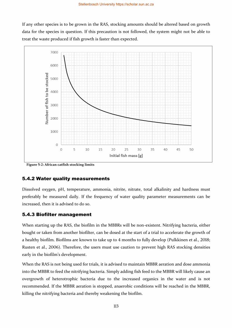
113

If any other species is to be grown in the RAS, stocking amounts should be altered based on growth

data for the species in question. If this precaution is not followed, the system might not be able to

treat the waste produced if fish growth is faster than expected.

Figure 5-2: African catfish stocking limits

5.4.2 Water quality measurements

Dissolved oxygen, pH, temperature, ammonia, nitrite, nitrate, total alkalinity and hardness must

preferably be measured daily. If the frequency of water quality parameter measurements can be

increased, then it is advised to do so.

5.4.3 Biofilter management

When starting up the RAS, the biofilm in the MBBRs will be non-existent. Nitrifying bacteria, either

bought or taken from another biofilter, can be dosed at the start of a trial to accelerate the growth of

a healthy biofilm. Biofilms are known to take up to 4 months to fully develop (Pulkkinen et al., 2018;

Rusten et al., 2006). Therefore, the users must use caution to prevent high RAS stocking densities

early in the biofilm’s development.

When the RAS is not being used for trials, it is advised to maintain MBBR aeration and dose ammonia

into the MBBR to feed the nitrifying bacteria. Simply adding fish feed to the MBBR will likely cause an

overgrowth of heterotrophic bacteria due to the increased organics in the water and is not

recommended. If the MBBR aeration is stopped, anaerobic conditions will be reached in the MBBR,

killing the nitrifying bacteria and thereby weakening the biofilm.


114

5.4.4 Flushing the lamella settler

Sludge from the lamella settler needs to be flushed daily to minimize ammonia leaching into the water

from the settled solids. Flushed solids must be disposed of according to local regulations. Details on

the disposal of the solids waste was out of the scope of this thesis. Regular checks of the plates inside

the lamella settler is recommended and these should be cleaned using a long brush on a weekly basis.

5.4.5 Make-up water

The RAS requires regular make-up water to prevent buildup of nitrate in the water. Assuming no

passive denitrification in the RAS, it was estimated that 332L of make-up water must be added for

every kg of feed fed. At peak design stocking density and biomass, the make-up water flow rate was

estimated to be 0.14 m3/h

5.4.6 Alkalinity dosing

Alkalinity dosing needs to be done to keep the pH balanced. Bovendeur et al. (1987) recommended 80

g NaHCO3 needs to be added per kg of feed. Regular pH measurements need to be done to ensure a

constant pH of 7.0.

5.4.7 Nitrite toxicity prevention

Nitrite can be extremely toxic to fish, even in low concentrations. The main method of preventing this

toxicity is by maintaining a sufficient chloride concentration in the water. The recommended ratio for

safe operation is a minimum of 20g Cl per g NO2-. As an additional safety margin, chloride

concentrations should be maintained at 100 mg/L. Salt (NaCl) can be added if the chloride

concentration is too low. Weekly chloride measurements are recommended.

5.4.8 Effects of overfeeding the system

Overfeeding of the RAS can occur if the maximum design biomass is exceeded or extreme feeding

levels are used. This will lead to the wastewater treatment units not removing waste at the same rate

as what is being produced since the units were designed for a certain feeding rate. Ultimately this

causes a net accumulation of waste products in the RAS and most importantly in the fish tanks. This

effect is shown in Figure 5-3 where the predicted increase in TAN concentration is shown in the days

following the peak loading.


115

Figure 5-3: Increase in TAN concentrations due to overfeeding

The rapid predicted increase in TAN concentrations in Figure 5-3 demonstrates the importance of

remaining below the design maximum feeding rate. This also shows that even though the biofilter is

oversized for most of the production period, an exceedance of the maximum design feeding rate will

quickly cause accumulation of TAN in the RAS.

5.4.9 Emergency power

Emergency power provided by a generator needs to be available in the case of power cuts.


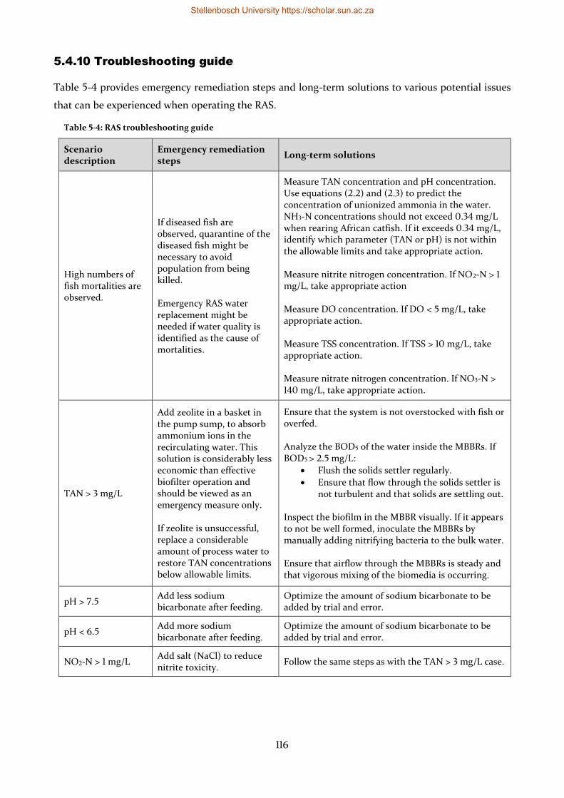
116

5.4.10 Troubleshooting guide

Table 5-4 provides emergency remediation steps and long-term solutions to various potential issues

that can be experienced when operating the RAS.

Table 5-4: RAS troubleshooting guide

Scenario description

Emergency remediation steps

Long-term solutions

High numbers of fish mortalities are observed.

If diseased fish are observed, quarantine of the diseased fish might be necessary to avoid population from being killed. Emergency RAS water replacement might be needed if water quality is identified as the cause of mortalities.

Measure TAN concentration and pH concentration. Use equations (2.2) and (2.3) to predict the concentration of unionized ammonia in the water. NH3-N concentrations should not exceed 0.34 mg/L when rearing African catfish. If it exceeds 0.34 mg/L, identify which parameter (TAN or pH) is not within the allowable limits and take appropriate action. Measure nitrite nitrogen concentration. If NO2-N > 1 mg/L, take appropriate action Measure DO concentration. If DO < 5 mg/L, take appropriate action. Measure TSS concentration. If TSS > 10 mg/L, take appropriate action. Measure nitrate nitrogen concentration. If NO3-N > 140 mg/L, take appropriate action.

TAN > 3 mg/L

Add zeolite in a basket in the pump sump, to absorb ammonium ions in the recirculating water. This solution is considerably less economic than effective biofilter operation and should be viewed as an emergency measure only. If zeolite is unsuccessful, replace a considerable amount of process water to restore TAN concentrations below allowable limits.

Ensure that the system is not overstocked with fish or overfed. Analyze the BOD5 of the water inside the MBBRs. If BOD5 > 2.5 mg/L:

• Flush the solids settler regularly.

• Ensure that flow through the solids settler is not turbulent and that solids are settling out.

Inspect the biofilm in the MBBR visually. If it appears to not be well formed, inoculate the MBBRs by manually adding nitrifying bacteria to the bulk water. Ensure that airflow through the MBBRs is steady and that vigorous mixing of the biomedia is occurring.

pH > 7.5 Add less sodium bicarbonate after feeding.

Optimize the amount of sodium bicarbonate to be added by trial and error.

pH < 6.5 Add more sodium bicarbonate after feeding.

Optimize the amount of sodium bicarbonate to be added by trial and error.

NO2-N > 1 mg/L Add salt (NaCl) to reduce nitrite toxicity.

Follow the same steps as with the TAN > 3 mg/L case.


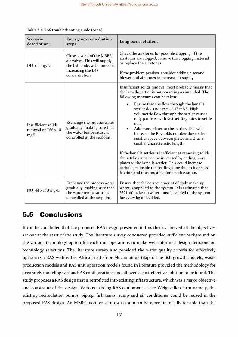
117

Table 5-4: RAS troubleshooting guide (cont.)

Scenario description

Emergency remediation steps

Long-term solutions

DO < 5 mg/L

Close several of the MBBR air valves. This will supply the fish tanks with more air, increasing the DO concentration.

Check the airstones for possible clogging. If the airstones are clogged, remove the clogging material or replace the air stones. If the problem persists, consider adding a second blower and airstones to increase air supply.

Insufficient solids removal or TSS > 10 mg/L

Exchange the process water gradually, making sure that the water temperature is controlled at the setpoint.

Insufficient solids removal most probably means that the lamella settler is not operating as intended. The following measures can be taken:

• Ensure that the flow through the lamella settler does not exceed 12 m3/h. High volumetric flow through the settler causes only particles with fast settling rates to settle out.

• Add more plates to the settler. This will increase the Reynolds number due to the smaller space between plates and thus a smaller characteristic length.

If the lamella settler is inefficient at removing solids, the settling area can be increased by adding more plates to the lamella settler. This could increase turbulence inside the settling zone due to increased friction and thus must be done with caution.

NO3-N > 140 mg/L

Exchange the process water gradually, making sure that the water temperature is controlled at the setpoint.

Ensure that the correct amount of daily make-up water is supplied to the system. It is estimated that 332L of make-up water must be added to the system for every kg of feed fed.

5.5 Conclusions

It can be concluded that the proposed RAS design presented in this thesis achieved all the objectives

set out at the start of the study. The literature survey conducted provided sufficient background on

the various technology option for each unit operations to make well-informed design decisions on

technology selections. The literature survey also provided the water quality criteria for effectively

operating a RAS with either African catfish or Mozambique tilapia. The fish growth models, waste

production models and RAS unit operation models found in literature provided the methodology for

accurately modeling various RAS configurations and allowed a cost-effective solution to be found. The

study proposes a RAS design that is retrofitted into existing infrastructure, which was a major objective

and constraint of the design. Various existing RAS equipment at the Welgevallen farm namely, the

existing recirculation pumps, piping, fish tanks, sump and air conditioner could be reused in the

proposed RAS design. An MBBR biofilter setup was found to be more financially feasible than the


118

existing trickling filters due to high pumping costs associated with the operation of the trickling filters.

Additionally, the high flow rate required for trickling filter operation dramatically increased the solids

settling unit size. The final objective was met by proposing an operating guide for effective operation

of the proposed RAS. Finally, it can be concluded by the author that the proposed design is ready for

implementation and the project is estimated to cost a total of approximately R 145 000.

5.6 Recommendations for process optimization

5.6.1 Floating feces technology

Since most TSS in water originate from feed excretion (Chen et al., 1994), research into floating feces

technology has been conducted (Unger and Brinker, 2013). It was found that certain feed additives

could lower the density of feces allowing it to float. The feces could then be easily removed by

screening or skimming equipment before breaking up into smaller particles which are more difficult

to remove. In a rainbow trout system, solids removal efficiency was found to increase from 25% to

59% when using floating feces feed additives (Schumann et al., 2017). No adverse effects on fish health

was observed when feed additives were used in rainbow trout feed (Unger and Brinker, 2013;

Schumann et al., 2017).

5.6.2 Automatic feeding

Feeding only 2 to 3 times a day (as is commonly done if manual feeding is employed during

experimental trials) can cause drastic fluctuations in waste products in the water. This is due to higher

mass of feed being fed at one time compared to if the feed is uniformly fed across 24 hours. This high

feed mass entering the system is often eaten quickly and digested before the next feeding event,

causing fluctuations in the waste stream entering the system. A solution to this is the use of automatic

feeders, which can be loaded with feed pellets and programmed to feed the fish uniformly across 24

hours, increasing the stability of waste product concentrations in the RAS. This solution is expensive

and should only be considered if the waste concentrations in the RAS is unstable and the user is sure

that the WWT units are operating efficiently.

5.6.3 Energy usage

Energy usage in RAS is a topic that is rarely covered in most articles. However, a recent review by

Badiola et al. (2018) on the topic of energy usage has identified several methods for reduction of energy

usage and costs:

• Exploiting the height difference between unit operations to reduce pumping costs.

• Use of geothermal energy for heating.

• Use of pure oxygen to reduce flow rate requirements and thus pumping costs.


119

• Limiting the use of fine solids filtration to side-streams, which can be used intermittently. This

can greatly reduce pumping costs due to the high head loss associated with fine solids

filtration. An exception to this is foam fractionation.

• Use of solar energy for heating through solar collectors and/or greenhouses.

• Utilization of thermal wastewater from nearby industries.

• Use of airlift pumps.

• Use of axial pumps with variable speed control to reduce pumping costs when system is not at

peak loading.

• Use of a surface aerator with variable speed control for carbon dioxide removal.

5.6.3.1 Blower air flow restriction

Process water heating requirements could be reduced be by restricting the blower air flow through the

fish tanks and MBBRs using a valve. Restricting air flow will decrease heat loss by evaporation and

decrease heat gains by heated blower air. Process water heating requirements would be reduced if

there is an overall decrease in net heat loss. However, restricting the regenerative blower air flow will

increase the current drawn by the blower motor, increasing energy usage. An investigation into these

opposing effects can be done to assess the energy savings of restricting air flow. Due to the dynamic

nature of the oxygen consumption through a trial, this optimization would be best done during

operations.

5.6.3.2 Water heating versus air heating

Process water heating requirements decrease at higher building air temperatures. This fact creates a

possible opportunity for optimization of energy usage by tuning the building air temperature set point

to minimize the process water heating. This is best done during operation as the air heating

requirements over time is difficult to model due to changing weather and solar heating of the building

air by solar radiation penetrating the greenhouse panels.

5.6.3.3 Solar water heating

Utilizing solar energy for water heating has become popular and is a possible way of reducing the

energy usage of the RAS (Fuller, 2007). Time series solar radiation data will need to be used in

conjunction with various solar heating setups to determine the investment with the shortest payback

period.

5.6.3.4 Variable speed drive pumps

As the operations in the proposed RAS will be for experimental trials, the stocking density and thus

the required recirculation flow rate will be low at the start of a trial and gradually increase along with

biomass increase as the trial progresses. Therefore, replacing the proposed recirculation pump with a

variable speed drive pump could potentially decrease overall power costs if operated correctly.

5.6.3.5 Insulation

Heat losses can be reduced by installing insulation around process water piping.


120

References

Adewolu, M.A., Adeniji, C.A., Adejobi, A.B., 2008. Feed utilization, growth and survival of Clarias gariepinus (Burchell 1822) fingerlings cultured under different photoperiods. Aquaculture 283, 64–67.

Akinwole, A.O., Faturoti, E.O., 2007. Biological performance of African Catfish (Clarias gariepinus) cultured in recirculating system in Ibadan. Aquac. Eng. 36, 18–23.

Al Ba’ba’a, H.B.M., 2015. A New Correlation for Predicting Aeration Efficiency for Air Diffused Systems. University of Wisconsin.

Alibaba, 2019. Food Grade Sodium Bicarbonate [WWW Document]. URL https://www.alibaba.com/product-detail/China-Supplier-Factory-Sale-Food-Grade_60601890252.html (accessed 10.2.19).

APHA, 1998. Standard Methods for Examination of Water and Wastewater, 20th ed, Standard Methods. Association American Public Health.

Aquarius Technologies Inc., 2011. Aeration upgrade - Western Riverside County Regional WW Authority. Carlsbad.

Arceivala, S.J., 1983. Discussion of “Hydraulic Modeling for Waste Stabilization Ponds” by Raymond A. Ferrara and Donald R. F. Harleman (August, 1981). J. Environ. Eng. 109, 265–268.

Ashley, K.I., Hall, K.J., Mavinic, D.S., 1991. Factors influencing oxygen transfer in fine pore diffused aeration. Water Res. 25, 1479–1486.

Baccarin, A.E., Camargo, A.F.M., 2005. Characterization and evaluation of the impact of feed management on the effluents of Nile tilapia (Oreochromis niloticus) culture. Brazilian Arch. Biol. Technol. 48, 81–90.

Badiola, M., Basurko, O.C., Piedrahita, R., Hundley, P., Mendiola, D., 2018. Energy use in Recirculating Aquaculture Systems (RAS): A review. Aquac. Eng. 81, 57–70.

Béné, C., Arthur, R., Norbury, H., Allison, E.H., Beveridge, M., Bush, S., Campling, L., Leschen, W., Little, D., Squires, D., Thilsted, S.H., Troell, M., Williams, M., 2016. Contribution of Fisheries and Aquaculture to Food Security and Poverty Reduction: Assessing the Current Evidence. World Dev. 79, 177–196.

Besson, M., Komen, H., Aubin, J., De Boer, I.J.M., Poelman, M., Quillet, E., Vancoillie, C., Vandeputte, M., Van Arendonk, J.A., 2014. Economic values of growth and feed efficiency for fish farming in recirculating aquaculture system with density and nitrogen output limitations: A case study with African catfish (clarias gariepinus). J. Anim. Sci. 92, 5394–5405.

Blancheton, J.P., Attramadal, K.J.K., Michaud, L., D’Orbcastel, E.R., Vadstein, O., 2013. Insight into bacterial population in aquaculture systems and its implication. Aquac. Eng. 53, 30–39.

Bovendeur, J., 1989. Fixed-biofilm reactors applied to waste water treatment and aquacultural water recirculating systems. Wageningen University.

Bovendeur, J., Eding, E.H., Henken, A.M., 1987. Design and performance of a water recirculation system for high-density culture of the African catfish, Clarias gariepinus (Burchell 1822). Aquaculture 63, 329–353.

Bovendeur, J., Klapwijk, A., 1986. Zuivering en recirculatie van water in visteeltsystemen 1. H2O 19, 136–140.

Brandt, M.J., Johnson, K.J., Elphinston, A.J., Ratnayaka, D.D., 2016. Twort’s Water Supply, 7th ed. Butterworth-Heinemann.

Brazil, B.L., 2006. Performance and operation of a rotating biological contactor in a tilapia


121

recirculating aquaculture system. Aquac. Eng. 34, 261–274.

Brazil, B.L., Summerfelt, S.T., Libey, G.S., 1996. Application of Ozone to Recirculating Aquaculture Systems, in: Successes and Failures in Commercial Recirculating Aquaculture.

Buentello, J.A., Gatlin, D.M., Neill, W.H., 2000. Effects of water temperature and dissolved oxygen on daily feed consumption, feed utilization and growth of channel catfish (Ictalurus punctatus). Aquaculture 182, 339–352.

Bureau, D., Azevedo, P., Tapia-salazar, M., Cuzon, G., 2000. Pattern and cost of growth and nutrient deposition in fish and shrimp: Potential implications and applications. Av. en Nutr. 111–140.

Buttle, L.G., Uglow, R., Cowx, I., 1995. Effect of dietary protein on the nitrogen excretion and growth of the African catfish, Clarias gariepinus. Aquat. Living Resour. 8, 407–414.

Camargo, J.A., Alonso, A., Salamanca, A., 2005. Nitrate toxicity to aquatic animals: a review with new data for freshwater invertebrates. Chemosphere 58, 1255–1267.

Caraman, S., Barbu, M., Ionescu, T., Ifrim, G., Cristea, V., Ceangǎ , E., 2010. The analysis of the dynamic properties of the wastewater treatment process in a recirculating aquaculture system. Rom. Biotechnol. Lett. 15, 5457–5466.

Çengel, J.A., Ghajar, A.J., 2013. Chapter 16: Heating and Cooling of Buildings, in: Heat and Mass Transfer: A Practical Approach.

Cengel, Y.A., Boles, M.A., 2015. Thermodynamics: An Engineering Approach, 8th ed. McGraw-Hill Education.

Cengel, Y.A., Cimbala, J.M., 2014. Fluid Mechanics: Fundamentals and Applications, 3rd ed. McGraw-Hill Education.

Cengel, Y.A., Ghajar, A.J., 2015. Heat and Mass Transfer: Fundamentals and Applications, 5th ed. McGraw-Hill Education, New York.

CFW Fans, 2019a. Regenerative blowers. Cape Town.

CFW Fans, 2019b. ZXB series catalogue: Side channel blowers and exhausters. Cape Town.

Chapman, P.M., Popham, J.D., Griffin, J., Leslie, D., Michaelson, J., 1987. Differentiation of physical from chemical toxicity in solid waste fish bioassays. Water. Air. Soil Pollut. 33, 295–308.

Chen, S., Coffin, D.E., Malone, R.F., 1993. Production, characteristics, and modeling of aquacultural sludge from a recirculating aquacultural system using a granular media biofilter, in: Wang, J.-K. (Ed.), Techniques for Modern Aquaculture. American Society of Agricultural Engineers, pp. 16–25.

Chen, S., Stechey, D., Malone, R.F., 1994. Suspended Solids Control in Recirculating Aquaculture Systems, in: Timmons, M.B., Losordo, T.M. (Eds.), Aquaculture Water Reuse Systems: Engineering Design and Management. Elsevier Science B.V., Amsterdam, pp. 61–100.

Colt, J.E., Tchobanoglous, G., 1981. Design of aeration systems for aquaculture, in: Proceedings of the Bioengineering Symposium for Fish Culture. American Fisheries Society, Bethesda, pp. 138–148.

d’Orbcastel, E.R., Blancheton, J., Aubin, J., 2009. Towards environmentally sustainable aquaculture: Comparison between two trout farming systems using Life Cycle Assessment. Aquac. Eng. 40, 113–119.

DAFF, 2018. African Sharptooth Catfish Feasibility Study [WWW Document]. URL https://www.nda.agric.za/doaDev/sideMenu/fisheries/03_areasofwork/Aquaculture/economics/Final Catfish Feasibility Study 2018_Formatted.pdf (accessed 7.31.19).

Davidson, J., Summerfelt, S.T., 2005. Solids removal from a coldwater recirculating system - Comparison of a swirl separator and a radial-flow settler. Aquac. Eng. 33, 47–61.


122

Degani, G., Ben-Zvi, Y., Levanon, D., 1989. The effect of different protein levels and temperatures on feed utilization, growth and body composition of Clarias gariepinus (Burchell 1822). Aquaculture 76, 293–301.

Drennan, D.G., Hosler, K.C., Francis, M., Weaver, D., Aneshansley, E., Beckman, G., Johnson, C.H., Cristina, C.M., 2006. Standardized evaluation and rating of biofilters. II. Manufacturer’s and user’s perspective. Aquac. Eng. 34, 403–416.

Dumas, A., France, J., Bureau, D., 2010. Modelling growth and body composition in fish nutrition: Where have we been and where are we going? Aquac. Res. 41, 161–181.

Dumas, A., France, J., Bureau, D.P., 2007. Evidence of three growth stanzas in rainbow trout (Oncorhynchus mykiss) across life stages and adaptation of the thermal-unit growth coefficient. Aquaculture 267, 139–146.

Easter, C., 1992. System component performance and water quality in a recirculating system produce hybrid striped bass, in: Aquacultural Expo V. New Orleans.

Ecotao Enterprises, 2019. Positive displacement blower: roots type [WWW Document]. URL https://www.ecotao.co.za/html/positivedisplacementblower.html (accessed 9.3.19).

Ecotao Enterprises, 2018a. Biomedia Quotation 2018/10/22.

Ecotao Enterprises, 2018b. Air stones - general stock.

Ecotao Enterprises, 2017. Biomedia Quotation 2017/02/15.

Eding, E.H., Kamstra, A., Verreth, J.A.J., Huisman, E.A., Klapwijk, A., 2006. Design and operation of nitrifying trickling filters in recirculating aquaculture: A review. Aquac. Eng. 34, 234–260.

Emerson, K., Russo, R.C., Lund, R.E., Thurston, R.V., 1975. Aqueous ammonia equilibrium calculations: Effect of pH and temperature. J. Fish. Res. Board Canada 32, 2379–2383.

FAOSTAT, 2017. FAO Yearbook: Fishery and Aquaculture Statistics. 2015, FAO Annual Yearbook.

Faraji, A., Asadollafardi, G., Shevidi, A., 2013. A pilot study for the application of one- and two-stage tube settlers as a secondary clarifier for wastewater treatment. Int. J. Civ. Eng. 11, 272–280.

Farhat, Khan, M.A., 2011. Growth, Feed Conversion, and Nutrient Retention Efficiency of African Catfish, Clarias gariepinus, (Burchell) Fingerling Fed Diets with Varying Levels of Protein. J. Appl. Aquac. 23, 304–316.

Fernandes, P., Pedersen, L.F., Pedersen, P.B., 2015. Microscreen effects on water quality in replicated recirculating aquaculture systems. Aquac. Eng. 65, 17–26.

Fernandes, P.M., Pedersen, L.F., Pedersen, P.B., 2017. Influence of fixed and moving bed biofilters on micro particle dynamics in a recirculating aquaculture system. Aquac. Eng. 78, 32–41.

Fernandes, P.M., Pedersen, L.F., Pedersen, P.B., 2014. Daily micro particle distribution of an experimental recirculating aquaculture system-A case study. Aquac. Eng. 60, 28–34.

Fogler, H.S., 2014. Elements of Chemical Reaction Engineering, 4th ed. Pearson.

Froese, R., 2006. Cube law, condition factor and weight–length relationships: history, meta-analysis and recommendations. J. Appl. Ichthyol. 22, 241–253.

Fuller, R.J., 2007. Solar heating systems for recirculation aquaculture. Aquac. Eng. 36, 250–260.

Futurama, 2019. Pond Medic 55W UV Sterilizer - 18000L/H [WWW Document]. URL https://www.futurama.co.za/pond-medic-55w-uv-sterilizer-18000l-h (accessed 10.2.19).

Gallert, C., Winter, J., 2008. Bacterial Metabolism in Wastewater Treatment Systems, Biotechnology: Second, Completely Revised Edition.

Gericke, S.J., 2019. The effects of xylanase and arabinoxylan- oligosaccharides on the growth performance , non- specific immunity , hindgut microbial diversity and hindgut short-chain fatty


123

acid production of African catfish , Clarias gariepinus by Master of Agricultural Sci.

Goosen, N.J., 2014. Investigation of potential bio- active properties and effects on production performance of aquafeed ingredients derived from fish processing waste by way of enzymatic autolysis 204.

Grace, G.., Piedrahita, R.H., 1994. Carbon Dioxide Control, in: Timmons, M.B., Losordo, T.M. (Eds.), Aquaculture Water Reuse Systems: Engineering Design and Management. Elsevier Science B.V., Amsterdam, pp. 209–234.

Gråkjær, 2019. Personal communication.

Greiner, A.D., Timmons, M.B., 1998. Evaluation of the nitrification rates of microbead and trickling filters in an intensive recirculating tilapia production facility. Aquac. Eng. 18, 189–200.

Grundfos, 2019. Grundfos Product Center [WWW Document]. URL product-selection.grundfos.com (accessed 10.1.19).

Guerdat, T.C., Losordo, T.M., Classen, J.J., Osborne, J.A., DeLong, D.P., 2010. An evaluation of commercially available biological filters for recirculating aquaculture systems. Aquac. Eng. 42, 38–49.

Hazen, A., 1904. On Sedimentation. Trans. ASCE.

Heinen, J.M., Hankins, J.A., Weber, A.L., Watten, B.J., 1996. A semi-closed recirculating water system for high-density culture of rainbow trout. Progress. Fish-Culturist 58, 11–22.

Hem, L.J., Rusten, B., Ødegaard, H., 1994. Nitrification in a moving bed biofilm reactor. Water Res. 28, 1425–1433.

Henze, M., Harremoës, P., la Cour Jansen, J., Arvin, E., 1997. Wastewater Treatment, 2nd ed. Springer, Berlin, Heidelberg, New York.

Henze, M., Jr, C.P.L.G., Gujer, W., Marais, G. v. R., Matsuo, T., 1987. Activated Sludge Model no. 1.

Hilmy, A.M., El-Domiaty, N.A., Wershana, K., 1987. Acute and chronic toxicity of nitrite to Clarias Lazera. Comp. Biochem. Physiol. - Part C Toxicol. Pharmacol. 86, 247–253.

Hochheimer, J.N., Wheaton, F., 2000. Biological Filters : Trickling and RBC Design 291–318.

Huguenin, J.E., Colt, J., 2002. Design and operating guide for aquaculture seawater systems. Elsevier.

Incropera, F.P., DeWitt, D.P., Bergman, T.L., Lavine, A.S., 2007. Fundamentals of Heat and Mass Transfer, 6th ed, International Journal of Heat and Mass Transfer. John Wiley & Sons.

Iwama, G.K., Tautz, A.F., 1981. A simple growth model for salmonids in hatcheries. Can. J. Fish. Aquat. Sci. 38, 649–656.

Kamstra, A., Blom, E., Terjesen, B.F., 2017. Mixing and scale affect moving bed biofilm reactor (MBBR) performance. Aquac. Eng. 78, 9–17.

Kamstra, A., van der Heul, J.., Nijhof, M., 1998. Performance and optimisation of trickling filters on eel farms. Aquac. Eng. 17, 175–192.

Karimanzira, D., Keesman, K.J., Kloas, W., Baganz, D., Rauschenbach, T., 2016. Dynamic modeling of the INAPRO aquaponic system. Aquac. Eng. 75, 29–45.

Kawan, J.A., Abu Hasan, H., Suja, F., Jaafar, O., Abd-Rahman, R., 2016. A review on sewage treatment and polishing using moving bed bioreactor (Mbbr). J. Eng. Sci. Technol. 11, 1098–1120.

Kinyage, J.P.H., Pedersen, L.F., 2016. Impact of temperature on ammonium and nitrite removal rates in RAS moving bed biofilters. Aquac. Eng. 75, 51–55.

Kroupova, H., Machova, J., Svobodova, Z., 2005. Nitrite influence on fish : a review. Vet Med 50, 461–471.


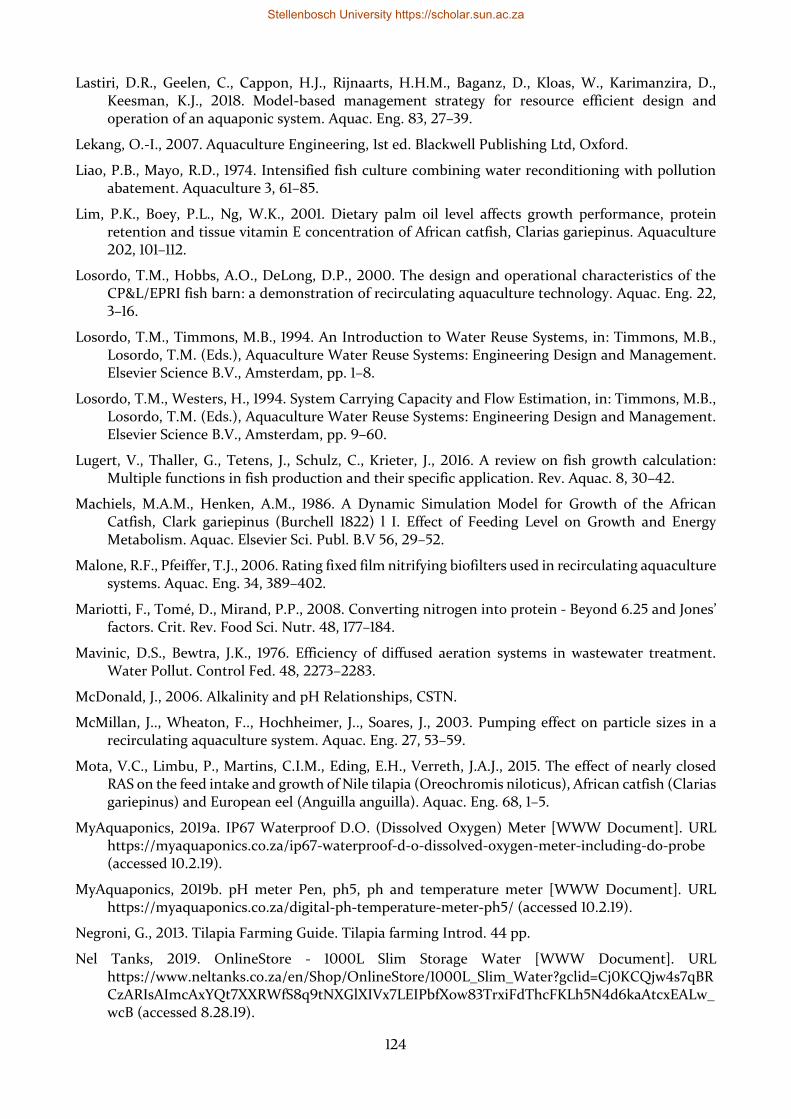
124

Lastiri, D.R., Geelen, C., Cappon, H.J., Rijnaarts, H.H.M., Baganz, D., Kloas, W., Karimanzira, D., Keesman, K.J., 2018. Model-based management strategy for resource efficient design and operation of an aquaponic system. Aquac. Eng. 83, 27–39.

Lekang, O.-I., 2007. Aquaculture Engineering, 1st ed. Blackwell Publishing Ltd, Oxford.

Liao, P.B., Mayo, R.D., 1974. Intensified fish culture combining water reconditioning with pollution abatement. Aquaculture 3, 61–85.

Lim, P.K., Boey, P.L., Ng, W.K., 2001. Dietary palm oil level affects growth performance, protein retention and tissue vitamin E concentration of African catfish, Clarias gariepinus. Aquaculture 202, 101–112.

Losordo, T.M., Hobbs, A.O., DeLong, D.P., 2000. The design and operational characteristics of the CP&L/EPRI fish barn: a demonstration of recirculating aquaculture technology. Aquac. Eng. 22, 3–16.

Losordo, T.M., Timmons, M.B., 1994. An Introduction to Water Reuse Systems, in: Timmons, M.B., Losordo, T.M. (Eds.), Aquaculture Water Reuse Systems: Engineering Design and Management. Elsevier Science B.V., Amsterdam, pp. 1–8.

Losordo, T.M., Westers, H., 1994. System Carrying Capacity and Flow Estimation, in: Timmons, M.B., Losordo, T.M. (Eds.), Aquaculture Water Reuse Systems: Engineering Design and Management. Elsevier Science B.V., Amsterdam, pp. 9–60.

Lugert, V., Thaller, G., Tetens, J., Schulz, C., Krieter, J., 2016. A review on fish growth calculation: Multiple functions in fish production and their specific application. Rev. Aquac. 8, 30–42.

Machiels, M.A.M., Henken, A.M., 1986. A Dynamic Simulation Model for Growth of the African Catfish, Clark gariepinus (Burchell 1822) l I. Effect of Feeding Level on Growth and Energy Metabolism. Aquac. Elsevier Sci. Publ. B.V 56, 29–52.

Malone, R.F., Pfeiffer, T.J., 2006. Rating fixed film nitrifying biofilters used in recirculating aquaculture systems. Aquac. Eng. 34, 389–402.

Mariotti, F., Tomé, D., Mirand, P.P., 2008. Converting nitrogen into protein - Beyond 6.25 and Jones’ factors. Crit. Rev. Food Sci. Nutr. 48, 177–184.

Mavinic, D.S., Bewtra, J.K., 1976. Efficiency of diffused aeration systems in wastewater treatment. Water Pollut. Control Fed. 48, 2273–2283.

McDonald, J., 2006. Alkalinity and pH Relationships, CSTN.

McMillan, J.., Wheaton, F.., Hochheimer, J.., Soares, J., 2003. Pumping effect on particle sizes in a recirculating aquaculture system. Aquac. Eng. 27, 53–59.

Mota, V.C., Limbu, P., Martins, C.I.M., Eding, E.H., Verreth, J.A.J., 2015. The effect of nearly closed RAS on the feed intake and growth of Nile tilapia (Oreochromis niloticus), African catfish (Clarias gariepinus) and European eel (Anguilla anguilla). Aquac. Eng. 68, 1–5.

MyAquaponics, 2019a. IP67 Waterproof D.O. (Dissolved Oxygen) Meter [WWW Document]. URL https://myaquaponics.co.za/ip67-waterproof-d-o-dissolved-oxygen-meter-including-do-probe (accessed 10.2.19).

MyAquaponics, 2019b. pH meter Pen, ph5, ph and temperature meter [WWW Document]. URL https://myaquaponics.co.za/digital-ph-temperature-meter-ph5/ (accessed 10.2.19).

Negroni, G., 2013. Tilapia Farming Guide. Tilapia farming Introd. 44 pp.

Nel Tanks, 2019. OnlineStore - 1000L Slim Storage Water [WWW Document]. URL https://www.neltanks.co.za/en/Shop/OnlineStore/1000L_Slim_Water?gclid=Cj0KCQjw4s7qBRCzARIsAImcAxYQt7XXRWfS8q9tNXGlXIVx7LEIPbfXow83TrxiFdThcFKLh5N4d6kaAtcxEALw_wcB (accessed 8.28.19).


125

NGMA, 2010. National Greenhouse Manufacturers Association standards for heat loss in greenhouse structures. Harrisburg.

Nijhof, M., 1995. Bacterial stratification and hydraulic loading effects in a plug-flow model for nitrifying trickling filters applied in recirculating fish culture systems. Aquaculture 134, 49–64.

Nijhof, M., Bovendeur, J., 1990. Fixed film nitrification characteristics in sea-water recirculation fish culture systems. Aquaculture 87, 133–143.

Ødegaard, H., 1995. Method for purification of water. 5,458,779.

Oluwaseyi, A.M., 2016. Application of dietary clay as feed additive on feed quality, water quality and production performance of African catfish (Clarias gariepinus). Stellenbosch University.

Palm, H.W., Knaus, U., Wasenitz, B., Bischoff, A.A., Strauch, S.M., 2018. Proportional up scaling of African catfish (Clarias gariepinus Burchell, 1822) commercial recirculating aquaculture systems disproportionally affects nutrient dynamics. Aquaculture 491, 155–168.

Palram, 2019. Multiwall Polycarbonate Sheets For Greenhouse [WWW Document]. URL https://www.palram.com/us/sub-product/thermaglas-polycarbonate-multi-wall/ (accessed 10.2.19).

Pfeiffer, T.J., Wills, P.S., 2011. Evaluation of three types of structured floating plastic media in moving bed biofilters for total ammonia nitrogen removal in a low salinity hatchery recirculating aquaculture system. Aquac. Eng. 45, 51–59.

Piedrahita, R.H., Seland, A., 1995. Calculation of pH in fresh and sea water aquaculture systems. Aquac. Eng. 14, 331–346.

Pruszyński, T., 2003. Effects of feeding on ammonium excretion and growth of the African catfish (Clarias gariepinus) fry. Czech J. Anim. Sci. 48, 106–112.

Pulkkinen, J.T., Kiuru, T., Aalto, S.L., Koskela, J., Vielma, J., 2018. Startup and effects of relative water renewal rate on water quality and growth of rainbow trout ( Oncorhynchus mykiss ) in a unique RAS research platform. Aquac. Eng. 82, 38–45.

Rahmatullah, R., Das, M., Rahmatullah, S.M., 2010. Suitable stocking density of tilapia in an aquaponic system. Fish. Res 14, 29–35.

Robinson, E.H., Li, M.H., 2010. Channel Catfish, Ictalurus punctatus, Size and Feed Conversion Ratio. J. World Aquac. Soc. 41, 829–833.

Rojas-Tirado, P., Pedersen, P.B., Pedersen, L.F., 2017. Bacterial activity dynamics in the water phase during start-up of recirculating aquaculture systems. Aquac. Eng. 78, 24–31.

Rusten, B., Eikebrokk, B., Ulgenes, Y., Lygren, E., 2006. Design and operations of the Kaldnes moving bed biofilm reactors. Aquac. Eng. 34, 322–331.

Rusten, B., Hem, L.J., Ødegaard, H., 1995. Nitrification of municipal wastewater in moving-bed biofilm reactors. Water Environ. Res. 67, 75–86.

Salhi, M., Bessonart, M., Chediak, G., Bellagamba, M., Carnevia, D., 2004. Growth, feed utilization and body composition of black catfish, Rhamdia quelen, fry fed diets containing different protein and energy levels. Aquaculture 231, 435–444.

SalmonBusiness, 2018. New land-based fish farm for sea trout planned in South Africa [WWW Document]. Press Release. URL https://salmonbusiness.com/new-land-based-farm-for-sea-trout-planned-in-south-africa/

SAURAN, 2019. Southern African Universities Radiometric Network [WWW Document]. URL http://www.sauran.net/ShowStation.aspx?station=4 (accessed 8.21.19).

Schneider, O., Sereti, V., Eding, E.H., Verreth, J.A.J., Klapwijk, B., 2007. Kinetics, design and biomass production of a bacteria reactor treating RAS effluent streams. Aquac. Eng. 36, 24–35.


126

Schram, E., Roques, J.A.C., Abbink, W., Spanings, T., de Vries, P., Bierman, S., de Vis, H. van, Flik, G., 2010. The impact of elevated water ammonia concentration on physiology, growth and feed intake of African catfish (Clarias gariepinus). Aquaculture 306, 108–115.

Schram, E., Roques, J.A.C., Abbink, W., Yokohama, Y., 2014. The impact of elevated water nitrate concentration on physiology , growth and feed intake of African catfish Clarias gariepinus ( Burchell 1822 ). Aquac. Res. 1499–1511.

Schumann, M., Unger, J., Brinker, A., 2017. Floating faeces: Effects on solid removal and particle size distribution in RAS. Aquac. Eng. 78, 75–84.

Seshadri, K., Williams, F.A., 1978. Laminar flow between parallel plates with injection of a reactant at high reynolds number. Int. J. Heat Mass Transf. 21, 251–253.

Shah, M.M., 2014. Methods for Calculation of Evaporation from Swimming Pools and Other Water Surfaces (PREPRINT). ASHRAE Trans. 120, 1–15.

Shelton, J.L., Boyd, C.E., 1983. Correction Factors for Calculating Oxygen-Transfer Rates of Pond Aerators. Trans. Am. Fish. Soc. 112, 120–122.

Stechey, D.M., Trudell, Y., 1990. Aquaculture wastewater treatment: Wastewater characterization and development of appropriate technologies for the New Brunswick smolt production industry.

Stenstrom, M.K., Gilbert, R.G., 1981. Effects of alpha, beta and theta factor upon the design, specification and operation of aeration systems. Water Res. 15, 643–654.

Stokes, G.G., 1851. X. On the effect of internal friction of fluids on the motion of pendulums. Trans. Cambridge Philos. Soc. 9, 52.

Strauch, S.M., Wenzel, L.C., Bischoff, A., Dellwig, O., Klein, J., Schüch, A., Wasenitz, B., Palm, H.W., 2018. Commercial African Catfish (Clarias gariepinus) recirculating aquaculture systems: Assessment of element and energy pathways with special focus on the phosphorus cycle. Sustain. 10.

Stumm, W., Morgan, J.J., 1995. Aquatic Chemistry: Chemical Equilibria and Rates in Natural Waters, 3rd ed. John Wiley & Sons.

Suhr, K.I., Pedersen, P.B., 2010. Nitrification in moving bed and fixed bed biofilters treating effluent water from a large commercial outdoor rainbow trout RAS. Aquac. Eng. 42, 31–37.

Summerfelt, S.T., 2006. Design and management of conventional fluidized-sand biofilters. Aquac. Eng. 34, 275–302.

Summerfelt, S.T., Wilton, G., Roberts, D., Rimmer, T., Fonkalsrud, K., 2004. Developments in recirculating systems for Arctic char culture in North America. Aquac. Eng. 30, 31–71.

Suresh, A. V., Lin, C.K., 1992. Effect of stocking density on water quality and production of red tilapia in a recirculated water system. Aquac. Eng. 11, 1–22.

Swanepoel, J.C., 2017. Determination of bioavailability and bioactivity of enzymatically hydrolysed fish protein and phosphates in the African catfish Clarias gariepinus. Stellenbosch University.

Takealot, 2019. Speck pumps sand filter [WWW Document]. URL https://www.takealot.com/speck-pumps-aquaswim-filter-high-rate-sand-filter-2 (accessed 9.1.19).

Talamuk, R., 2016. Comparisons of Growth Performance of African Catfish Fingerlings Fed Different Inclusion Levels of Black Soldier Fly Larvae Meal Diets. Stellenbosch University.

Talati, S., 1988. Heat Loss in Aeration Tanks. University of California.

Terjesen, B.F., Summerfelt, S.T., Nerland, S., Ulgenes, Y., Fjæra, S.O., Megård Reiten, B.K., Selset, R., Kolarevic, J., Brunsvik, P., Bæverfjord, G., Takle, H., Kittelsen, A.H., Åsgård, T., 2013. Design, dimensioning, and performance of a research facility for studies on the requirements of fish in RAS environments. Aquac. Eng. 54, 49–63.


127

Timmons, M.B., 1994. Use Of Foam Fractionators in Aquaculture, in: Timmons, M.B., Losordo, T.M. (Eds.), Aquaculture Water Reuse Systems: Engineering Design and Management. Elsevier Science B.V., Amsterdam, pp. 247–280.

Timmons, M.B., Ebeling, J.M., 2007. Recirculating Aquaculture. Cayuga Aqua Ventures.

Tomasso, J.R., Simco, B.A., Davis, K.B., 1979. Chloride Inhibition of Nitrite-Induced Methemoglobinemia in Channel Catfish (Icalurus punctatus). J. Fish. Res. Board Canada 36, 1141–1144.

Torreele, E., Sluiszen, A. van Der, Verreth, J., 1993. The effect of dietary L-carnitine on the growth performance in fingerlings of the african catfish ( Clarias gariepinus ) in relation to dietary lipid. Br. J. Nutr. 69, 289–299.

Tran-Duy, A., Schrama, J.W., van Dam, A.A., Verreth, J.A.J., 2008. Effects of oxygen concentration and body weight on maximum feed intake, growth and hematological parameters of Nile tilapia, Oreochromis niloticus. Aquaculture 275, 152–162.

Unger, J., Brinker, A., 2013. Floating feces: A new approach for efficient removal of solids in aquacultural management. Aquaculture 404–405, 85–94.

Vaisala, 2013. Humidity conversion formulas - Calculation formulas for humidity. Helsinki.

van de Nieuwegiessen, P.G., Boerlage, A.S., Verreth, J.A.J., Schrama, J.W., 2008. Assessing the effects of a chronic stressor, stocking density, on welfare indicators of juvenile African catfish, Clarias gariepinus Burchell. Appl. Anim. Behav. Sci. 115, 233–243.

van de Nieuwegiessen, P.G., Olwo, J., Khong, S., Verreth, J.A.J., Schrama, J.W., 2009. Effects of age and stocking density on the welfare of African catfish, Clarias gariepinus Burchell. Aquaculture 288, 69–75.

Van Gorder, S.D., Jug-Dujakovic, J., 2004. Performance characteristics of rotating biological contactors within two commercial recirculating aquaculture systems, in: Proceedings of the Fifth International Conference on Recirculating Aquaculture. pp. 22–24.

Van Rijn, J., 2013. Waste treatment in recirculating aquaculture systems. Aquac. Eng. 53, 49–56.

van Weerd, J.H., Khalaf, K.H.A., Aartsen, F.J., Tijssen, P.A.T., 2003. Balance trials with African catfish Clarias gariepinus fed phytase-treated soybean meal-based diets. Aquac. Nutr. 5, 135–142.

Vinci, B.J., Timmons, M.B., Summerfelt, S.T., Watten, B.J., 1996. Carbon Dioxide Control in Intensive Aquaculture: Design Tool Development. AES Tech. Sess. 1 Open Pap.

Watanabe, W.O., Losordo, T.M., Fitzsimmons, K., Hanley, F., 2002. Tilapia Production Systems in the Americas: Technological Advances, Trends, and Challenges. Rev. Fish. Sci. 10, 465–498.

Watten, B.J., 1994. Aeration and Oxygenation, in: Timmons, M.B., Losordo, T.M. (Eds.), Aquaculture Water Reuse Systems: Engineering Design and Management. Elsevier Science B.V., Amsterdam, pp. 173–208.

Weitkamp, D.E., Katz, M., 1980. A review of dissolved gas supersaturation literature. Trans. Am. Fish. Soc. 109, 659–702.

Wheaton, F.., Hochheimer, J.., Kaiser, G.E., Krones, M.J., Libey, G.S., Easter, C.C., 1994a. Nitrification filter principles, in: Timmons, M.B., Losordo, T.M. (Eds.), Aquaculture Water Reuse Systems: Engineering Design and Management. Elsevier Science B.V., Amsterdam, pp. 101–126.

Wheaton, F.., Hochheimer, J., Kaiser, G.E., Malone, R.F., Krones, M.J., Libey, G.S., Easter, C.C., 1994b. Nitrification Filter Design Methods, in: Timmons, M.B., Losordo, T.M. (Eds.), Aquaculture Water Reuse Systems: Engineering Design and Management. Elsevier Science B.V., Amsterdam, pp. 127–172.

Wik, T., 1999. On Modeling the Dynamics of Fixed Biofilm Reactors. Chalmers University of


128

Technology.

Wik, T., Lindén, B., 2004. Modeling, control and simulation of recirculating aquaculture systems. IFAC Proc. Vol. 37, 141–146.

Wik, T.E.I., Lindén, B.T., Wramner, P.I., 2009. Integrated dynamic aquaculture and wastewater treatment modelling for recirculating aquaculture systems. Aquaculture 287, 361–370.

Wills, B.A., Finch, J.A., 2016. Wills’ Mineral Processing Technology, 8th ed. Elsevier Ltd.

Wong, K.B., Piedrahita, R.H., 2000. Settling velocity characterization of aquacultural solids. Aquac. Eng. 21, 233–246.

World Bank, 2011. The global program on fisheries: Strategic vision for fisheries and aquaculture.

Wortman, B., Wheaton, F., 1991. Temperature effects on biodrum nitrification. Aquac. Eng. 10, 183–205.

Yogev, U., Sowers, K.R., Mozes, N., Gross, A., 2017. Nitrogen and carbon balance in a novel near-zero water exchange saline recirculating aquaculture system. Aquaculture 467, 118–126.

Zhang, N., Wang, Z., 2017. Review of soil thermal conductivity and predictive models. Int. J. Therm. Sci. 117, 172–183.

Zhang, S.Y., Li, G., Wu, H.B., Liu, X.G., Yao, Y.H., Tao, L., Liu, H., 2011. An integrated recirculating aquaculture system (RAS) for land-based fish farming: The effects on water quality and fish production. Aquac. Eng. 45, 93–102.

Zhu, S., Chen, S., 2002. The impact of temperature on nitrification rate in fixed film biofilters. Aquac. Eng. 26.

Zhu, S., Chen, S., 2001. Effects of organic carbon on nitrification rate in fixed film biofilters. Aquac. Eng. 25, 1–11.


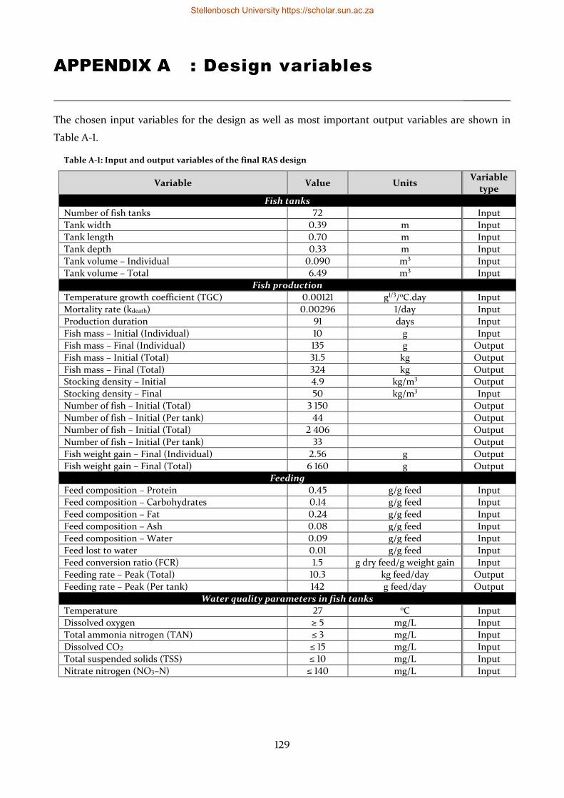
129

: Design variables

_________

The chosen input variables for the design as well as most important output variables are shown in

Table A-1.

Table A-1: Input and output variables of the final RAS design

Variable Value Units Variable

type

Fish tanks

Number of fish tanks 72 Input

Tank width 0.39 m Input

Tank length 0.70 m Input

Tank depth 0.33 m Input

Tank volume – Individual 0.090 m3 Input

Tank volume – Total 6.49 m3 Input

Fish production

Temperature growth coefficient (TGC) 0.00121 g1/3/oC.day Input

Mortality rate (kdeath) 0.00296 1/day Input

Production duration 91 days Input

Fish mass – Initial (Individual) 10 g Input

Fish mass – Final (Individual) 135 g Output

Fish mass – Initial (Total) 31.5 kg Output

Fish mass – Final (Total) 324 kg Output

Stocking density – Initial 4.9 kg/m3 Output

Stocking density – Final 50 kg/m3 Input

Number of fish – Initial (Total) 3 150 Output

Number of fish – Initial (Per tank) 44 Output

Number of fish – Initial (Total) 2 406 Output

Number of fish – Initial (Per tank) 33 Output

Fish weight gain – Final (Individual) 2.56 g Output

Fish weight gain – Final (Total) 6 160 g Output

Feeding

Feed composition – Protein 0.45 g/g feed Input

Feed composition – Carbohydrates 0.14 g/g feed Input

Feed composition – Fat 0.24 g/g feed Input

Feed composition – Ash 0.08 g/g feed Input

Feed composition – Water 0.09 g/g feed Input

Feed lost to water 0.01 g/g feed Input

Feed conversion ratio (FCR) 1.5 g dry feed/g weight gain Input

Feeding rate – Peak (Total) 10.3 kg feed/day Output

Feeding rate – Peak (Per tank) 142 g feed/day Output

Water quality parameters in fish tanks

Temperature 27 oC Input

Dissolved oxygen ≥ 5 mg/L Input

Total ammonia nitrogen (TAN) ≤ 3 mg/L Input

Dissolved CO2 ≤ 15 mg/L Input

Total suspended solids (TSS) ≤ 10 mg/L Input

Nitrate nitrogen (NO3–N) ≤ 140 mg/L Input


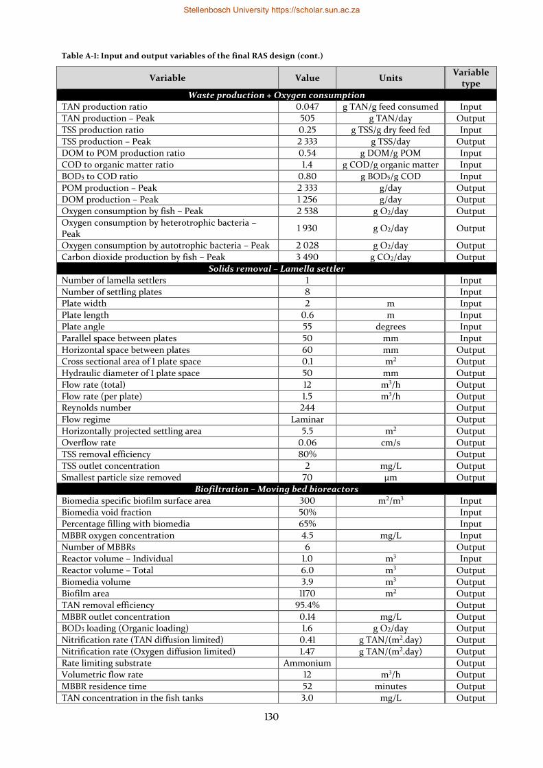
130

Table A-1: Input and output variables of the final RAS design (cont.)


type

Waste production + Oxygen consumption

TAN production ratio 0.047 g TAN/g feed consumed Input

TAN production – Peak 505 g TAN/day Output

TSS production ratio 0.25 g TSS/g dry feed fed Input

TSS production – Peak 2 333 g TSS/day Output

DOM to POM production ratio 0.54 g DOM/g POM Input

COD to organic matter ratio 1.4 g COD/g organic matter Input

BOD5 to COD ratio 0.80 g BOD5/g COD Input

POM production – Peak 2 333 g/day Output

DOM production – Peak 1 256 g/day Output

Oxygen consumption by fish – Peak 2 538 g O2/day Output

Oxygen consumption by heterotrophic bacteria – Peak

1 930 g O2/day Output

Oxygen consumption by autotrophic bacteria – Peak 2 028 g O2/day Output

Carbon dioxide production by fish – Peak 3 490 g CO2/day Output

Solids removal – Lamella settler

Number of lamella settlers 1 Input

Number of settling plates 8 Input

Plate width 2 m Input

Plate length 0.6 m Input

Plate angle 55 degrees Input

Parallel space between plates 50 mm Input

Horizontal space between plates 60 mm Output

Cross sectional area of 1 plate space 0.1 m2 Output

Hydraulic diameter of 1 plate space 50 mm Output

Flow rate (total) 12 m3/h Output

Flow rate (per plate) 1.5 m3/h Output

Reynolds number 244 Output

Flow regime Laminar Output

Horizontally projected settling area 5.5 m2 Output

Overflow rate 0.06 cm/s Output

TSS removal efficiency 80% Output

TSS outlet concentration 2 mg/L Output

Smallest particle size removed 70 μm Output

Biofiltration – Moving bed bioreactors

Biomedia specific biofilm surface area 300 m2/m3 Input

Biomedia void fraction 50% Input

Percentage filling with biomedia 65% Input

MBBR oxygen concentration 4.5 mg/L Input

Number of MBBRs 6 Output

Reactor volume – Individual 1.0 m3 Input

Reactor volume – Total 6.0 m3 Output

Biomedia volume 3.9 m3 Output

Biofilm area 1170 m2 Output

TAN removal efficiency 95.4% Output

MBBR outlet concentration 0.14 mg/L Output

BOD5 loading (Organic loading) 1.6 g O2/day Output

Nitrification rate (TAN diffusion limited) 0.41 g TAN/(m2.day) Output

Nitrification rate (Oxygen diffusion limited) 1.47 g TAN/(m2.day) Output

Rate limiting substrate Ammonium Output

Volumetric flow rate 12 m3/h Output

MBBR residence time 52 minutes Output

TAN concentration in the fish tanks 3.0 mg/L Output


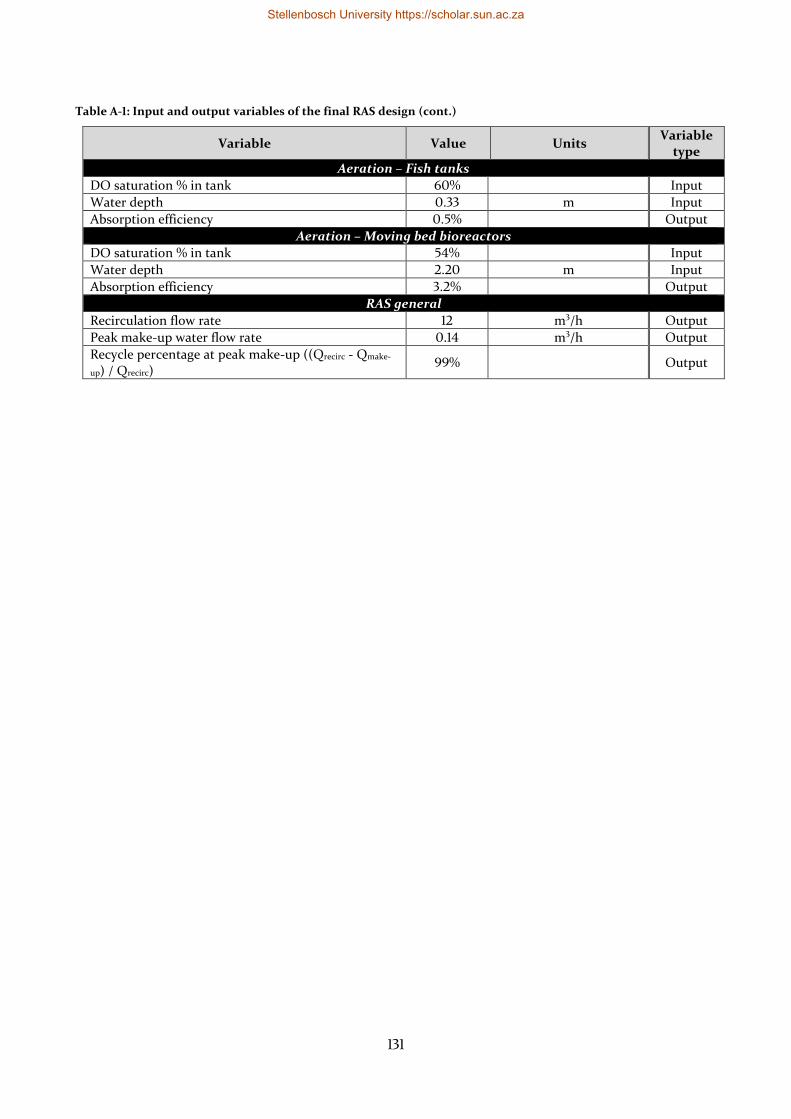
131

Table A-1: Input and output variables of the final RAS design (cont.)


type

Aeration – Fish tanks

DO saturation % in tank 60% Input

Water depth 0.33 m Input

Absorption efficiency 0.5% Output

Aeration – Moving bed bioreactors

DO saturation % in tank 54% Input

Water depth 2.20 m Input

Absorption efficiency 3.2% Output

RAS general

Recirculation flow rate 12 m3/h Output

Peak make-up water flow rate 0.14 m3/h Output

Recycle percentage at peak make-up ((Qrecirc - Qmake-

up) / Qrecirc) 99% Output


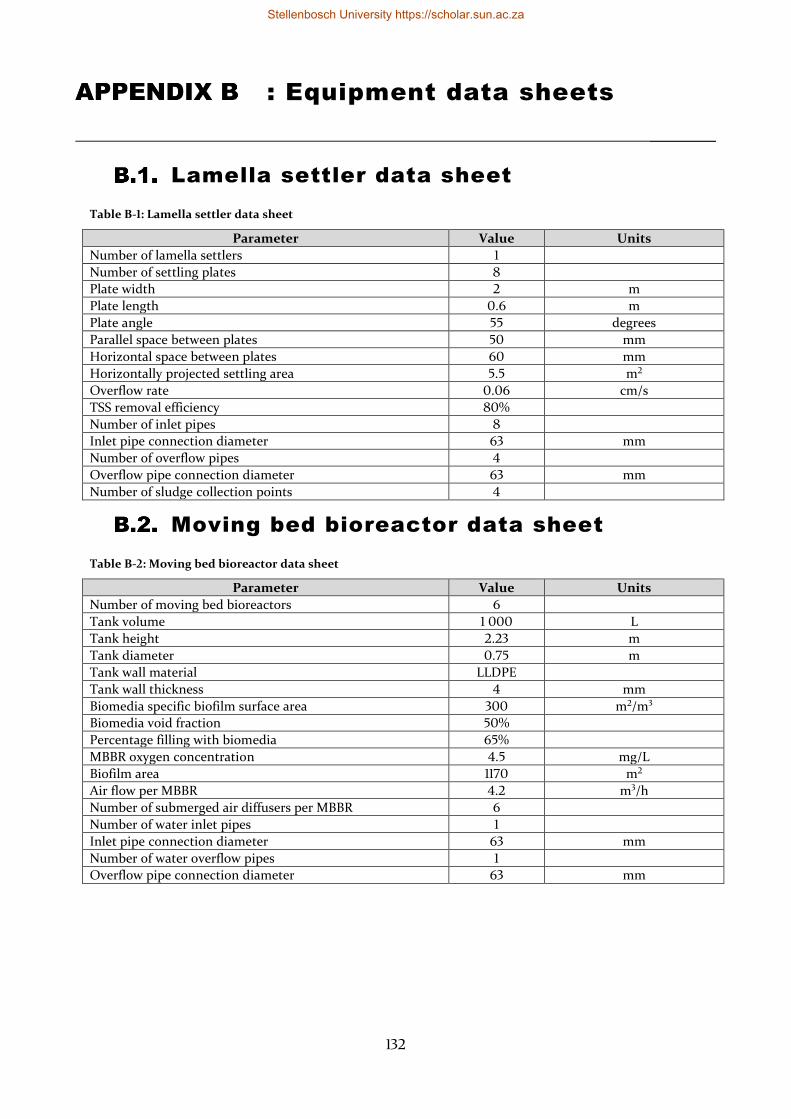
132

: Equipment data sheets

_________

Lamella settler data sheet

Table B-1: Lamella settler data sheet

Parameter Value Units

Number of lamella settlers 1

Number of settling plates 8

Plate width 2 m

Plate length 0.6 m

Plate angle 55 degrees

Parallel space between plates 50 mm

Horizontal space between plates 60 mm

Horizontally projected settling area 5.5 m2

Overflow rate 0.06 cm/s

TSS removal efficiency 80%

Number of inlet pipes 8

Inlet pipe connection diameter 63 mm

Number of overflow pipes 4

Overflow pipe connection diameter 63 mm

Number of sludge collection points 4

Moving bed bioreactor data sheet

Table B-2: Moving bed bioreactor data sheet


Number of moving bed bioreactors 6

Tank volume 1 000 L

Tank height 2.23 m

Tank diameter 0.75 m

Tank wall material LLDPE

Tank wall thickness 4 mm

Biomedia specific biofilm surface area 300 m2/m3

Biomedia void fraction 50%

Percentage filling with biomedia 65%

MBBR oxygen concentration 4.5 mg/L

Biofilm area 1170 m2

Air flow per MBBR 4.2 m3/h

Number of submerged air diffusers per MBBR 6

Number of water inlet pipes 1

Inlet pipe connection diameter 63 mm

Number of water overflow pipes 1

Overflow pipe connection diameter 63 mm


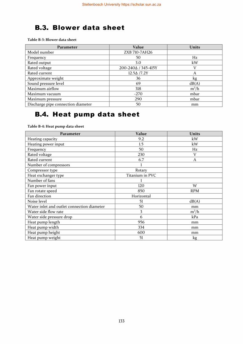
133

Blower data sheet

Table B-3: Blower data sheet


Model number ZXB 710-7AH26

Frequency 50 Hz

Rated output 3.0 kW

Rated voltage 200-240Δ / 345-415Y V

Rated current 12.5Δ /7.2Y A

Approximate weight 36 kg

Sound pressure level 69 dB(A)

Maximum airflow 318 m3/h

Maximum vacuum -270 mbar

Maximum pressure 290 mbar

Discharge pipe connection diameter 50 mm

Heat pump data sheet

Table B-4: Heat pump data sheet


Heating capacity 9.2 kW

Heating power input 1.5 kW

Frequency 50 Hz

Rated voltage 230 V

Rated current 6.7 A

Number of compressors 1

Compressor type Rotary

Heat exchanger type Titanium in PVC

Number of fans 1

Fan power input 120 W

Fan rotate speed 850 RPM

Fan direction Horizontal

Noise level 51 dB(A)

Water inlet and outlet connection diameter 50 mm

Water side flow rate 3 m3/h

Water side pressure drop 6 kPa

Heat pump length 956 mm

Heat pump width 334 mm

Heat pump height 600 mm

Heat pump weight 51 kg


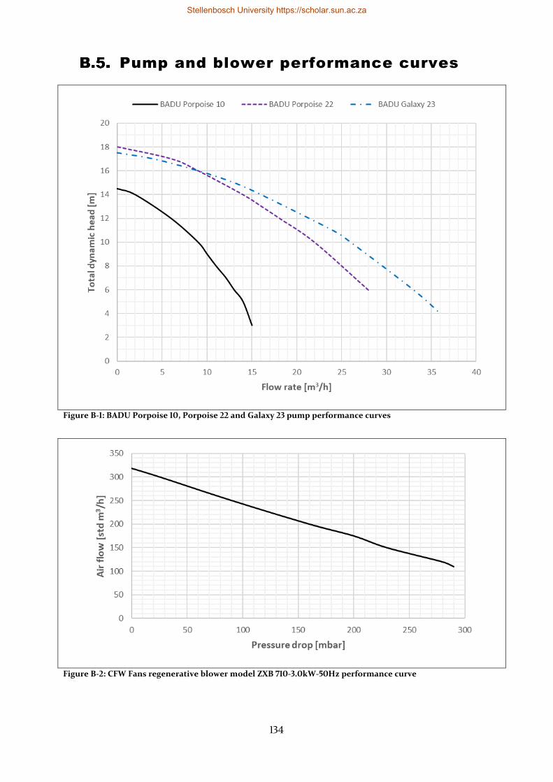
134

Pump and blower performance curves

Figure B-1: BADU Porpoise 10, Porpoise 22 and Galaxy 23 pump performance curves

Figure B-2: CFW Fans regenerative blower model ZXB 710-3.0kW-50Hz performance curve


135

Figure B-3: SCL V4 1.1kW-50Hz regenerative blower performance curve


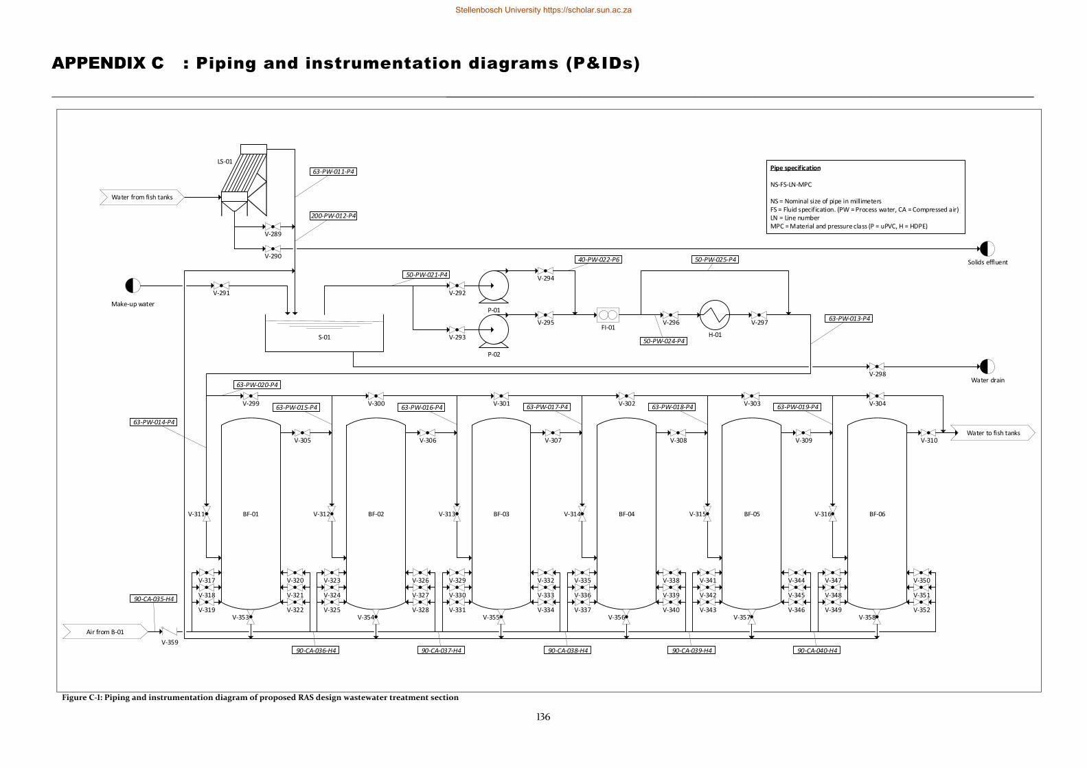
136

: Piping and instrumentation diagrams (P&IDs)

_____________________________________________________________________________________________________________________

Figure C-1: Piping and instrumentation diagram of proposed RAS design wastewater treatment section

H-01S-01

LS-01

Solids effluent

V-289

V-290

P-01

P-02

V-292

V-294

V-295

V-293

40-PW-022-P6

50-PW-021-P4

Make-up water

V-291

V-296 V-297

V-299

FI-01

V-300

V-311

V-305

Water from fish tanks

63-PW-011-P4

50-PW-025-P4

V-353V-319

BF-01

V-318

V-317 V-320

V-321

V-322

Air from B-01

V-325

V-324

V-323

BF-02V-312

63-PW-020-P4

V-326

V-327

V-328 V-331

V-330

V-329

BF-03V-313

V-332

V-333

V-334 V-337

V-336

V-335

BF-04V-314

V-338

V-339

V-340 V-343

V-342

V-341

BF-05V-315

V-344

V-345

V-346 V-349

V-348

V-347

BF-06V-316

V-350

V-351

V-352

90-CA-036-H4

V-354 V-355 V-356 V-357 V-358

V-301 V-302 V-303 V-304

V-306 V-307 V-308 V-309 V-310Water to fish tanks

Water drainV-298

63-PW-014-P4

63-PW-015-P4

V-359

90-CA-035-H4

200-PW-012-P4

63-PW-013-P4

63-PW-016-P4 63-PW-017-P4 63-PW-018-P4 63-PW-019-P4

50-PW-024-P4

90-CA-037-H4 90-CA-038-H4 90-CA-039-H4 90-CA-040-H4

Pipe specification

NS-FS-LN-MPC

NS = Nominal size of pipe in millimetersFS = Fluid specification. (PW = Process water, CA = Compressed air)LN = Line numberMPC = Material and pressure class (P = uPVC, H = HDPE)


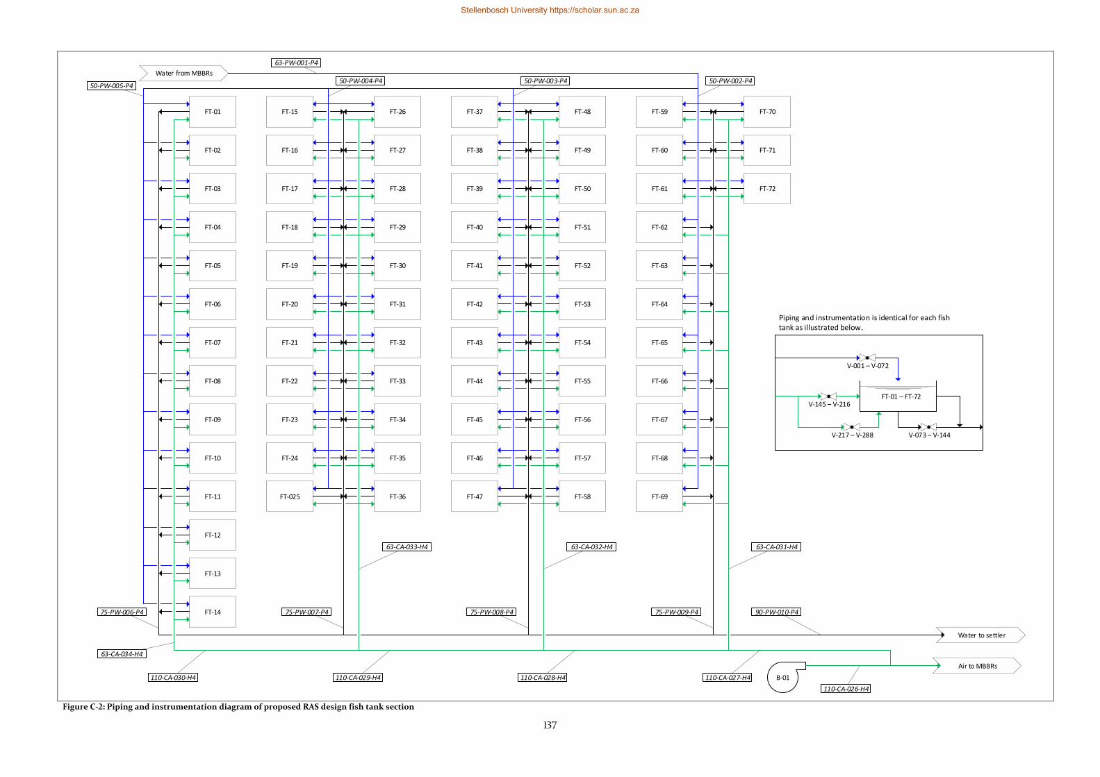
137

Figure C-2: Piping and instrumentation diagram of proposed RAS design fish tank section

B-01

Water from MBBRs

Air to MBBRs

Water to settler

FT-01 – FT-72V-145 – V-216

V-217 – V-288 V-073 – V-144

63-PW-001-P4

110-CA-026-H4

FT-14

FT-13

FT-12

FT-11

FT-10

FT-09

FT-08

FT-07

FT-06

FT-05

FT-04

FT-03

FT-02

FT-01

50-PW-005-P4

FT-15 FT-26 FT-37 FT-48 FT-59 FT-70

FT-16

FT-17

FT-18

FT-19

FT-20

FT-21

FT-22

FT-23

FT-24

FT-025

FT-27

FT-28

FT-29

FT-30

FT-31

FT-32

FT-33

FT-34

FT-35

FT-36

FT-38

FT-39

FT-40

FT-41

FT-42

FT-43

FT-44

FT-45

FT-46

FT-47

FT-49

FT-50

FT-51

FT-52

FT-53

FT-54

FT-55

FT-56

FT-57

FT-58

FT-60

FT-61

FT-62

FT-63

FT-64

FT-65

FT-66

FT-67

FT-68

FT-69

FT-71

FT-72

75-PW-006-P4 90-PW-010-P4

110-CA-027-H4

63-CA-031-H4

50-PW-003-P4 50-PW-002-P4

V-001 – V-072

Piping and instrumentation is identical for each fish tank as illustrated below.

50-PW-004-P4

75-PW-007-P4 75-PW-008-P4 75-PW-009-P4

110-CA-028-H4110-CA-029-H4

63-CA-034-H4

110-CA-030-H4

63-CA-032-H463-CA-033-H4


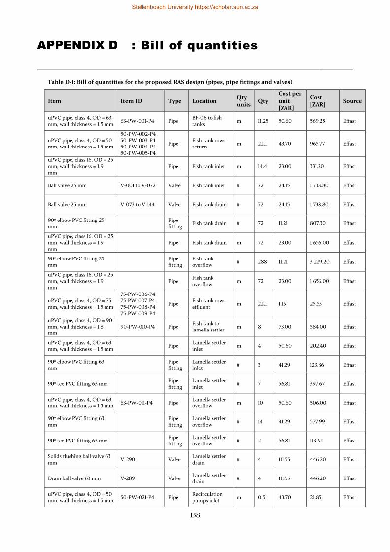
138

: Bill of quantities

_________

Table D-1: Bill of quantities for the proposed RAS design (pipes, pipe fittings and valves)

Item Item ID Type Location Qty units

Qty Cost per unit [ZAR]

Cost [ZAR]

Source

uPVC pipe, class 4, OD = 63 mm, wall thickness = 1.5 mm

63-PW-001-P4 Pipe BF-06 to fish tanks

m 11.25 50.60 569.25 Effast


50-PW-002-P4 50-PW-003-P4 50-PW-004-P4 50-PW-005-P4

Pipe Fish tank rows return

m 22.1 43.70 965.77 Effast


Pipe Fish tank inlet m 14.4 23.00 331.20 Effast

Ball valve 25 mm V-001 to V-072 Valve Fish tank inlet # 72 24.15 1 738.80 Effast

Ball valve 25 mm V-073 to V-144 Valve Fish tank drain # 72 24.15 1 738.80 Effast

90o elbow PVC fitting 25 mm

Pipe fitting

Fish tank drain # 72 11.21 807.30 Effast


Pipe Fish tank drain m 72 23.00 1 656.00 Effast


Pipe fitting

Fish tank overflow

# 288 11.21 3 229.20 Effast


Pipe Fish tank overflow

m 72 23.00 1 656.00 Effast


75-PW-006-P4 75-PW-007-P4 75-PW-008-P4 75-PW-009-P4

Pipe Fish tank rows effluent

m 22.1 1.16 25.53 Effast


90-PW-010-P4 Pipe Fish tank to lamella settler

m 8 73.00 584.00 Effast


Pipe Lamella settler inlet

m 4 50.60 202.40 Effast


Pipe fitting

Lamella settler inlet

# 3 41.29 123.86 Effast

90o tee PVC fitting 63 mm Pipe fitting

Lamella settler inlet

# 7 56.81 397.67 Effast


63-PW-011-P4 Pipe Lamella settler overflow

m 10 50.60 506.00 Effast


Pipe fitting

Lamella settler overflow

# 14 41.29 577.99 Effast

90o tee PVC fitting 63 mm Pipe fitting

Lamella settler overflow

# 2 56.81 113.62 Effast

Solids flushing ball valve 63 mm

V-290 Valve Lamella settler drain

# 4 111.55 446.20 Effast

Drain ball valve 63 mm V-289 Valve Lamella settler drain

# 4 111.55 446.20 Effast


50-PW-021-P4 Pipe Recirculation pumps inlet

m 0.5 43.70 21.85 Effast


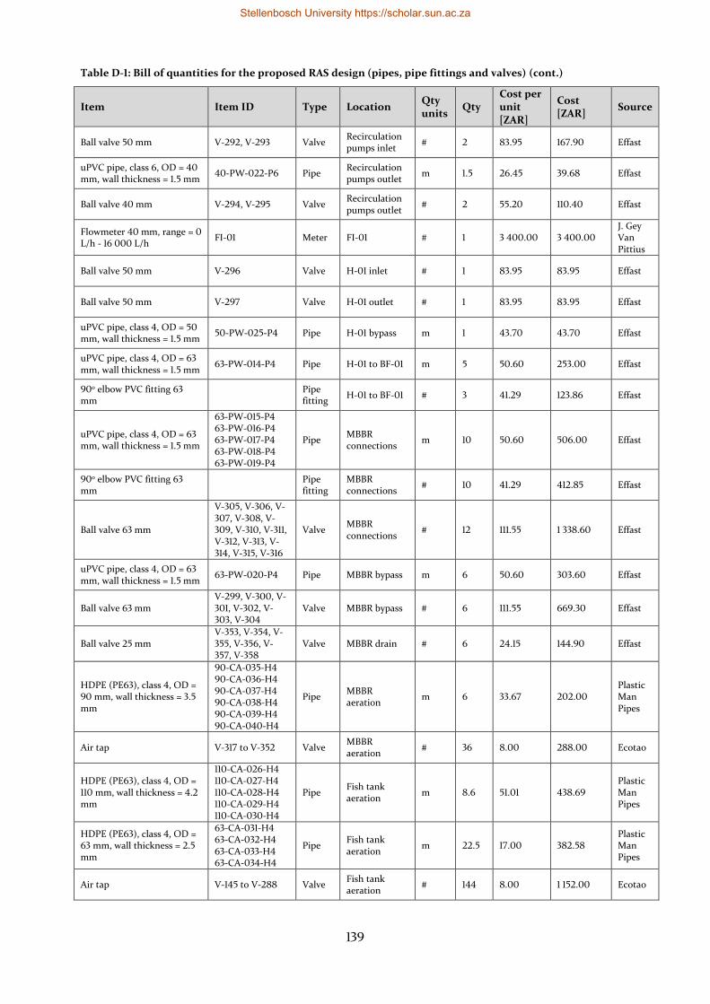
139

Table D-1: Bill of quantities for the proposed RAS design (pipes, pipe fittings and valves) (cont.)

Item Item ID Type Location Qty units

Qty Cost per unit [ZAR]

Cost [ZAR]

Source

Ball valve 50 mm V-292, V-293 Valve Recirculation pumps inlet

# 2 83.95 167.90 Effast


40-PW-022-P6 Pipe Recirculation pumps outlet

m 1.5 26.45 39.68 Effast

Ball valve 40 mm V-294, V-295 Valve Recirculation pumps outlet

# 2 55.20 110.40 Effast

Flowmeter 40 mm, range = 0 L/h - 16 000 L/h

FI-01 Meter FI-01 # 1 3 400.00 3 400.00 J. Gey Van Pittius

Ball valve 50 mm V-296 Valve H-01 inlet # 1 83.95 83.95 Effast

Ball valve 50 mm V-297 Valve H-01 outlet # 1 83.95 83.95 Effast


50-PW-025-P4 Pipe H-01 bypass m 1 43.70 43.70 Effast


63-PW-014-P4 Pipe H-01 to BF-01 m 5 50.60 253.00 Effast


Pipe fitting

H-01 to BF-01 # 3 41.29 123.86 Effast


63-PW-015-P4 63-PW-016-P4 63-PW-017-P4 63-PW-018-P4 63-PW-019-P4

Pipe MBBR connections

m 10 50.60 506.00 Effast


Pipe fitting

MBBR connections

# 10 41.29 412.85 Effast

Ball valve 63 mm

V-305, V-306, V-307, V-308, V-309, V-310, V-311, V-312, V-313, V-314, V-315, V-316

Valve MBBR connections

# 12 111.55 1 338.60 Effast


63-PW-020-P4 Pipe MBBR bypass m 6 50.60 303.60 Effast

Ball valve 63 mm V-299, V-300, V-301, V-302, V-303, V-304

Valve MBBR bypass # 6 111.55 669.30 Effast

Ball valve 25 mm V-353, V-354, V-355, V-356, V-357, V-358

Valve MBBR drain # 6 24.15 144.90 Effast

HDPE (PE63), class 4, OD = 90 mm, wall thickness = 3.5 mm

90-CA-035-H4 90-CA-036-H4 90-CA-037-H4 90-CA-038-H4 90-CA-039-H4 90-CA-040-H4

Pipe MBBR aeration

m 6 33.67 202.00 Plastic Man Pipes

Air tap V-317 to V-352 Valve MBBR aeration

# 36 8.00 288.00 Ecotao


110-CA-026-H4 110-CA-027-H4 110-CA-028-H4 110-CA-029-H4 110-CA-030-H4

Pipe Fish tank aeration

m 8.6 51.01 438.69 Plastic Man Pipes


63-CA-031-H4 63-CA-032-H4 63-CA-033-H4 63-CA-034-H4

Pipe Fish tank aeration

m 22.5 17.00 382.58 Plastic Man Pipes

Air tap V-145 to V-288 Valve Fish tank aeration

# 144 8.00 1 152.00 Ecotao


140

: Carbonate reaction equilibria

_________

Carbon dioxide gas dissolved in water (𝐶𝑂2(𝑎𝑞)) can react with water in a series of hydration and acid-

base reactions to form 𝐻2𝐶𝑂3(𝑎𝑞), 𝐻𝐶𝑂3(𝑎𝑞)− and 𝐶𝑂3(𝑎𝑞)

2− (Stumm and Morgan, 1995).

Carbonic acid is often represented by 𝐻2𝐶𝑂3∗ which includes both carbonic acid and dissolved carbon

dioxide:

[𝐻2𝐶𝑂3∗] = [𝐻2𝐶𝑂3(𝑎𝑞)] + [𝐶𝑂2(𝑎𝑞)]

The following equilibrium reactions describe the carbonate equilibria of the water (McDonald, 2006;

Stumm and Morgan, 1995).

Reaction 1: 𝐻2𝐶𝑂3∗ ↔ 𝐻𝐶𝑂3(𝑎𝑞)

− + 𝐻(𝑎𝑞)+ occurs at 4.3 < pH < 8.3

Reaction 2: 𝐻𝐶𝑂3(𝑎𝑞)− ↔ 𝐶𝑂3(𝑎𝑞)

2− + 𝐻(𝑎𝑞)+ occurs at 8.3 < pH < 10.2

Reaction W: 𝐻2𝑂(𝑙) ↔ 𝑂𝐻(𝑎𝑞)− + 𝐻(𝑎𝑞)

+ occurs at pH > 10.2


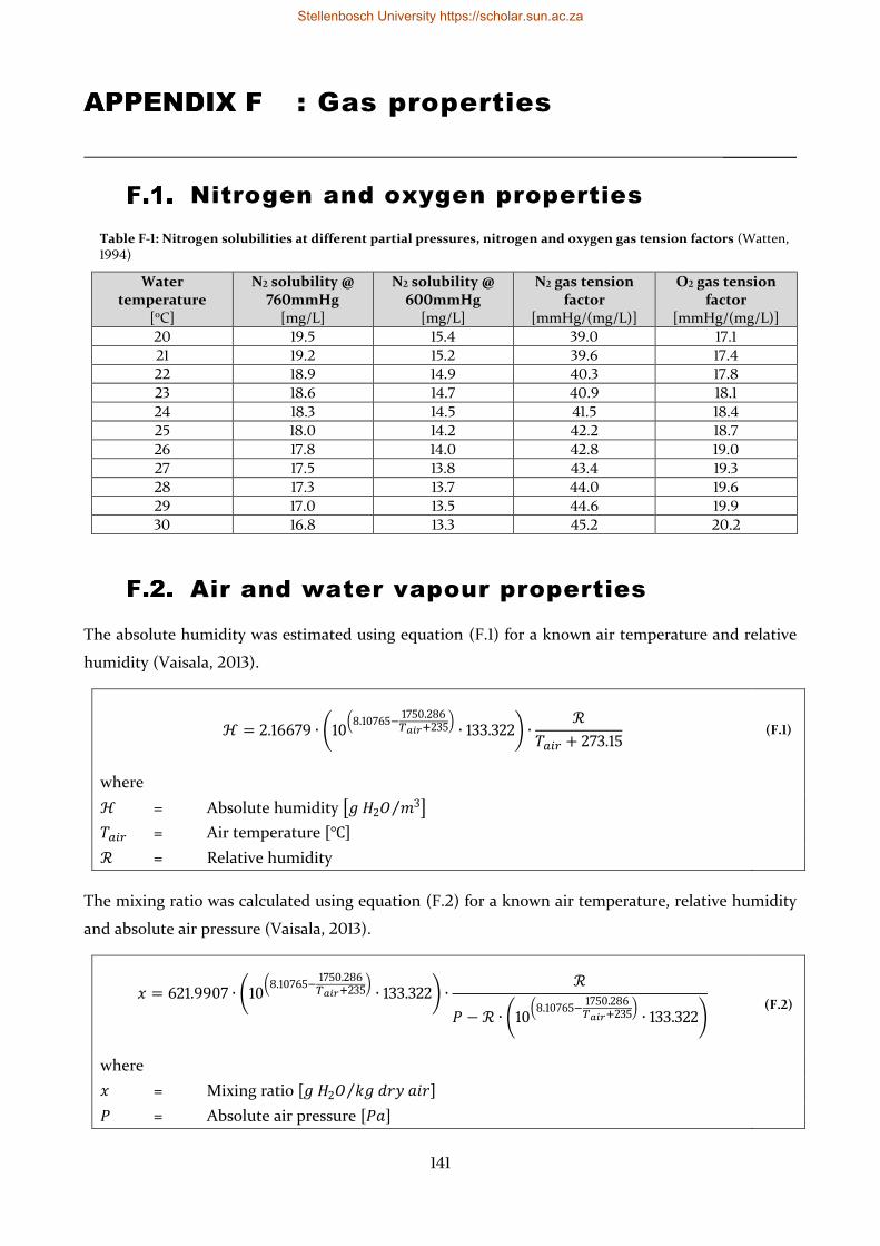
141

: Gas properties

_________

Nitrogen and oxygen properties

Table F-1: Nitrogen solubilities at different partial pressures, nitrogen and oxygen gas tension factors (Watten, 1994)

Water temperature

[oC]

N2 solubility @ 760mmHg

[mg/L]

N2 solubility @ 600mmHg

[mg/L]

N2 gas tension factor

[mmHg/(mg/L)]

O2 gas tension factor

[mmHg/(mg/L)]

20 19.5 15.4 39.0 17.1

21 19.2 15.2 39.6 17.4

22 18.9 14.9 40.3 17.8

23 18.6 14.7 40.9 18.1

24 18.3 14.5 41.5 18.4

25 18.0 14.2 42.2 18.7

26 17.8 14.0 42.8 19.0

27 17.5 13.8 43.4 19.3

28 17.3 13.7 44.0 19.6

29 17.0 13.5 44.6 19.9

30 16.8 13.3 45.2 20.2

Air and water vapour properties

The absolute humidity was estimated using equation (F.1) for a known air temperature and relative

humidity (Vaisala, 2013).

ℋ = 2.16679 ∙ (10(8.10765−

1750.286𝑇𝑎𝑖𝑟+235

)∙ 133.322) ∙

ℛ

𝑇𝑎𝑖𝑟 + 273.15 (F.1)

where

ℋ = Absolute humidity [𝑔 𝐻2𝑂 𝑚3⁄ ]

𝑇𝑎𝑖𝑟 = Air temperature [℃]

ℛ = Relative humidity

The mixing ratio was calculated using equation (F.2) for a known air temperature, relative humidity

and absolute air pressure (Vaisala, 2013).

𝑥 = 621.9907 ∙ (10(8.10765−

1750.286𝑇𝑎𝑖𝑟+235

)∙ 133.322) ∙

ℛ

𝑃 − ℛ ∙ (10(8.10765−

1750.286𝑇𝑎𝑖𝑟+235

)∙ 133.322)

(F.2)

where

𝑥 = Mixing ratio [𝑔 𝐻2𝑂 𝑘𝑔 𝑑𝑟𝑦 𝑎𝑖𝑟⁄ ]

𝑃 = Absolute air pressure [𝑃𝑎]


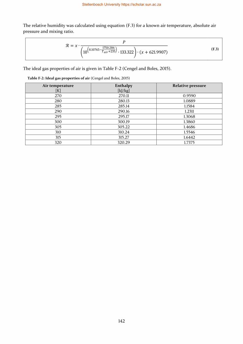
142

The relative humidity was calculated using equation (F.3) for a known air temperature, absolute air

pressure and mixing ratio.

ℛ = 𝑥 ∙𝑃

(10(8.10765−

1750.286𝑇𝑎𝑖𝑟+235

)∙ 133.322) ∙ (𝑥 + 621.9907)

(F.3)

The ideal gas properties of air is given in Table F-2 (Cengel and Boles, 2015).

Table F-2: Ideal gas properties of air (Cengel and Boles, 2015)

Air temperature [K]

Enthalpy [kJ/kg]

Relative pressure

270 270.11 0.9590

280 280.13 1.0889

285 285.14 1.1584

290 290.16 1.2311

295 295.17 1.3068

300 300.19 1.3860

305 305.22 1.4686

310 310.24 1.5546

315 315.27 1.6442

320 320.29 1.7375


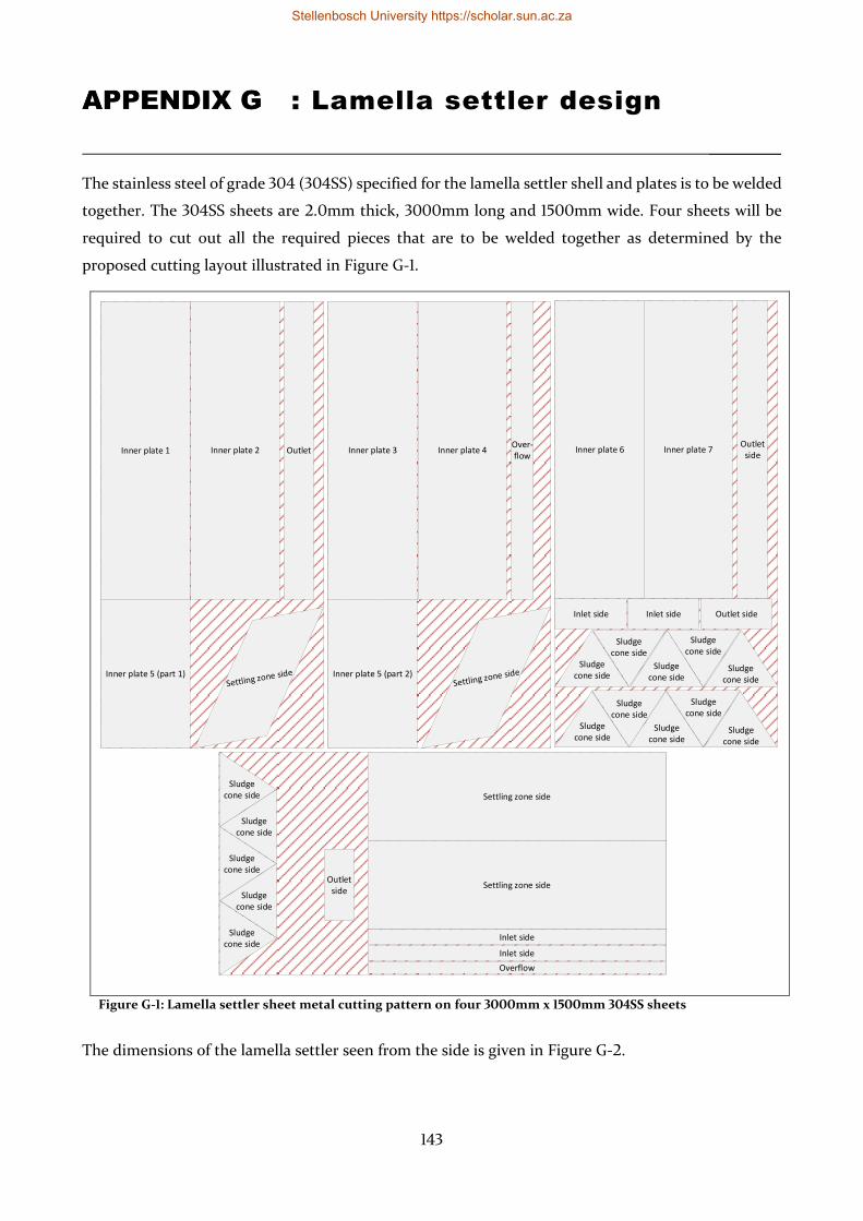
143

: Lamella settler design

_________

The stainless steel of grade 304 (304SS) specified for the lamella settler shell and plates is to be welded

together. The 304SS sheets are 2.0mm thick, 3000mm long and 1500mm wide. Four sheets will be

required to cut out all the required pieces that are to be welded together as determined by the

proposed cutting layout illustrated in Figure G-1.

Figure G-1: Lamella settler sheet metal cutting pattern on four 3000mm x 1500mm 304SS sheets

The dimensions of the lamella settler seen from the side is given in Figure G-2.

Settling zone side

Settling zone side

Outlet side

Inlet side

Inner plate 1 Inner plate 2 Inner plate 3 Inner plate 4 Inner plate 6 Inner plate 7

Inner plate 5 (part 1) Inner plate 5 (part 2)

Inlet side

Inlet side

Outlet side

Inlet side Outlet side

Sludge cone side

Sludge cone side

Sludge cone side

Sludge cone side

Sludge cone side

Sludge cone side

Sludge cone side

Sludge cone side

Sludge cone side

Sludge cone side

Sludge cone side

Sludge cone side

Sludge cone side

Sludge cone side

Sludge cone side

Outlet

Overflow

Over-flow


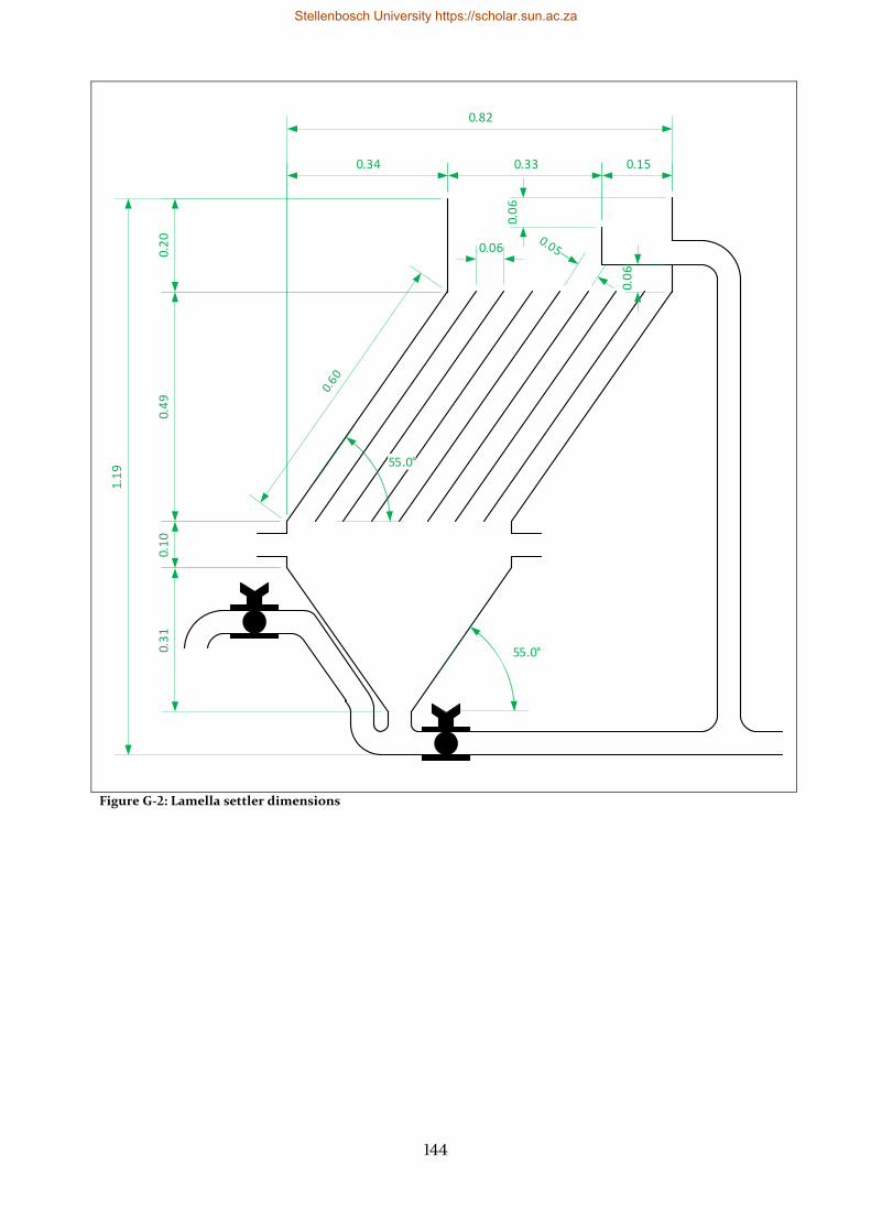
144

Figure G-2: Lamella settler dimensions

0.34 0.33

0.06

0.3

1

55.0°

0.1

00.

49

0.2

00.15

0.0

6

0.0

6

55.0°

1.1

90.82


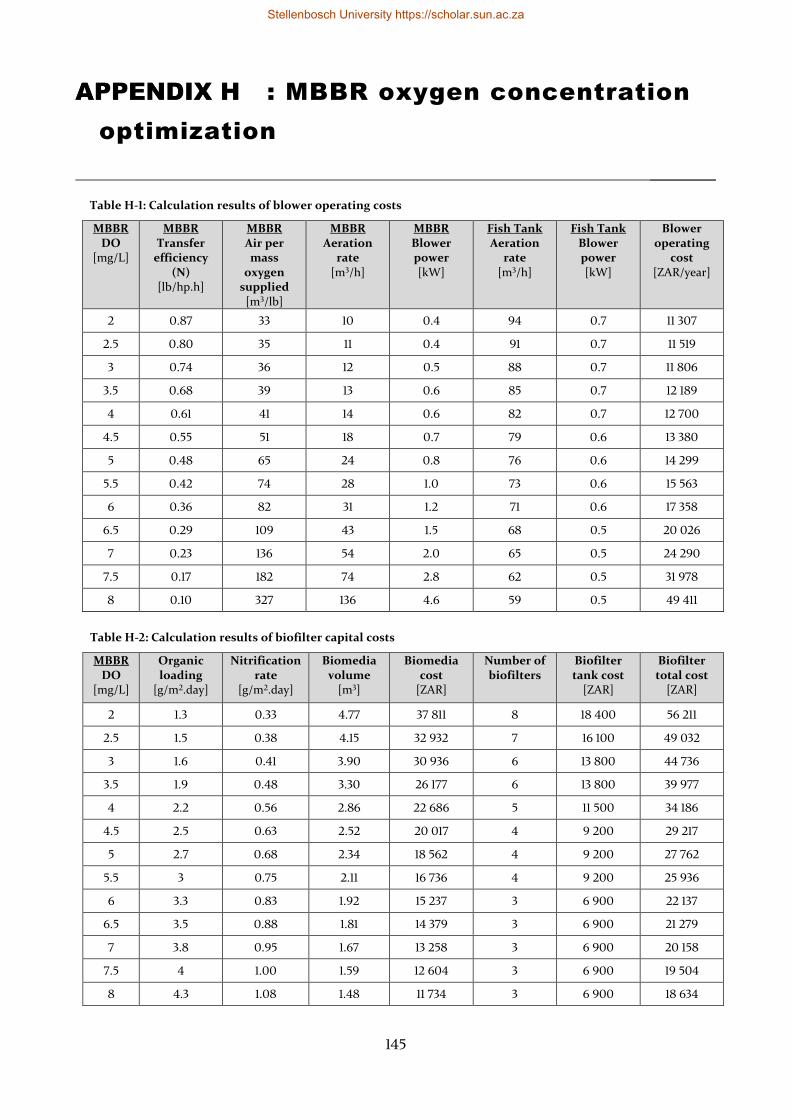
145

: MBBR oxygen concentration

optimization

_________

Table H-1: Calculation results of blower operating costs

MBBR DO

[mg/L]

MBBR Transfer

efficiency (N)

[lb/hp.h]

MBBR Air per mass

oxygen supplied [m3/lb]

MBBR Aeration

rate [m3/h]

MBBR Blower power [kW]

Fish Tank Aeration

rate [m3/h]

Fish Tank Blower power [kW]

Blower operating

cost [ZAR/year]

2 0.87 33 10 0.4 94 0.7 11 307

2.5 0.80 35 11 0.4 91 0.7 11 519

3 0.74 36 12 0.5 88 0.7 11 806

3.5 0.68 39 13 0.6 85 0.7 12 189

4 0.61 41 14 0.6 82 0.7 12 700

4.5 0.55 51 18 0.7 79 0.6 13 380

5 0.48 65 24 0.8 76 0.6 14 299

5.5 0.42 74 28 1.0 73 0.6 15 563

6 0.36 82 31 1.2 71 0.6 17 358

6.5 0.29 109 43 1.5 68 0.5 20 026

7 0.23 136 54 2.0 65 0.5 24 290

7.5 0.17 182 74 2.8 62 0.5 31 978

8 0.10 327 136 4.6 59 0.5 49 411

Table H-2: Calculation results of biofilter capital costs

MBBR DO

[mg/L]

Organic loading

[g/m2.day]

Nitrification rate

[g/m2.day]

Biomedia volume

[m3]

Biomedia cost

[ZAR]

Number of biofilters

Biofilter tank cost

[ZAR]

Biofilter total cost

[ZAR]

2 1.3 0.33 4.77 37 811 8 18 400 56 211

2.5 1.5 0.38 4.15 32 932 7 16 100 49 032

3 1.6 0.41 3.90 30 936 6 13 800 44 736

3.5 1.9 0.48 3.30 26 177 6 13 800 39 977

4 2.2 0.56 2.86 22 686 5 11 500 34 186

4.5 2.5 0.63 2.52 20 017 4 9 200 29 217

5 2.7 0.68 2.34 18 562 4 9 200 27 762

5.5 3 0.75 2.11 16 736 4 9 200 25 936

6 3.3 0.83 1.92 15 237 3 6 900 22 137

6.5 3.5 0.88 1.81 14 379 3 6 900 21 279

7 3.8 0.95 1.67 13 258 3 6 900 20 158

7.5 4 1.00 1.59 12 604 3 6 900 19 504

8 4.3 1.08 1.48 11 734 3 6 900 18 634


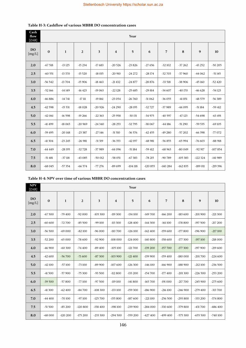
146

Table H-3: Cashflow of various MBBR DO concentration cases

Cash flow

[ZAR] Year

DO [mg/L]

0 1 2 3 4 5 6 7 8 9 10

2.0 -67 518 -13 125 -15 234 -17 683 -20 526 -23 826 -27 656 -32 102 -37 262 -43 252 -50 205

2.5 -60 551 -13 370 -15 520 -18 015 -20 910 -24 272 -28 174 -32 703 -37 960 -44 062 -51 145

3.0 -56 542 -13 704 -15 906 -18 463 -21 432 -24 877 -28 876 -33 518 -38 906 -45 160 -52 420

3.5 -52 166 -14 149 -16 423 -19 063 -22 128 -25 685 -29 814 -34 607 -40 170 -46 628 -54 123

4.0 -46 886 -14 741 -17 111 -19 861 -23 054 -26 760 -31 062 -36 055 -41 851 -48 579 -56 389

4.5 -42 598 -15 531 -18 028 -20 926 -24 290 -28 195 -32 727 -37 989 -44 095 -51 184 -59 412

5.0 -42 061 -16 598 -19 266 -22 363 -25 958 -30 131 -34 975 -40 597 -47 123 -54 698 -63 491

5.5 -41 499 -18 065 -20 969 -24 340 -28 253 -32 795 -38 067 -44 186 -51 290 -59 535 -69 105

6.0 -39 495 -20 148 -23 387 -27 146 -31 510 -36 576 -42 455 -49 280 -57 202 -66 398 -77 072

6.5 -41 304 -23 245 -26 981 -31 319 -36 353 -42 197 -48 981 -56 855 -65 994 -76 603 -88 918

7.0 -44 449 -28 195 -32 728 -37 989 -44 096 -51 184 -59 412 -68 963 -80 049 -92 917 -107 854

7.5 -51 481 -37 118 -43 085 -50 012 -58 051 -67 383 -78 215 -90 789 -105 383 -122 324 -141 989

8.0 -68 045 -57 354 -66 574 -77 276 -89 699 -104 118 -120 855 -140 284 -162 835 -189 011 -219 396

Table H-4: NPV over time of various MBBR DO concentration cases

NPV [ZAR]

Year

DO [mg/L]

0 1 2 3 4 5 6 7 8 9 10

2.0 -67 500 -79 400 -92 000 -105 300 -119 300 -134 100 -149 700 -166 200 -183 600 -201 900 -221 300

2.5 -60 600 -72 700 -85 500 -99 100 -113 300 -128 400 -144 300 -161 100 -178 800 -197 500 -217 200

3.0 -56 500 -69 000 -82 100 -96 000 -110 700 -126 100 -142 400 -159 600 -177 800 -196 900 -217 100

3.5 -52 200 -65 000 -78 600 -92 900 -108 000 -124 000 -140 800 -158 600 -177 300 -197 100 -218 000

4.0 -46 900 -60 300 -74 400 -89 400 -105 100 -121 700 -139 200 -157 700 -177 300 -197 900 -219 600

4.5 -42 600 -56 700 -71 600 -87 300 -103 900 -121 400 -139 900 -159 400 -180 000 -201 700 -224 600

5.0 -42 100 -57 100 -73 100 -89 900 -107 600 -126 300 -146 100 -166 900 -188 900 -212 100 -236 500

5.5 -41 500 -57 900 -75 300 -93 500 -112 800 -133 200 -154 700 -177 400 -201 300 -226 500 -253 200

6.0 -39 500 -57 800 -77 100 -97 500 -119 100 -141 800 -165 700 -191 000 -217 700 -245 900 -275 600

6.5 -41 300 -62 400 -84 700 -108 300 -133 100 -159 300 -186 900 -216 100 -246 900 -279 400 -313 700

7.0 -44 400 -70 100 -97 100 -125 700 -155 800 -187 600 -221 100 -256 500 -293 800 -333 200 -374 800

7.5 -51 500 -85 200 -120 800 -158 400 -198 100 -239 900 -284 000 -330 600 -379 800 -431 700 -486 400

8.0 -68 000 -120 200 -175 200 -233 300 -294 500 -359 200 -427 400 -499 400 -575 300 -655 500 -740 100


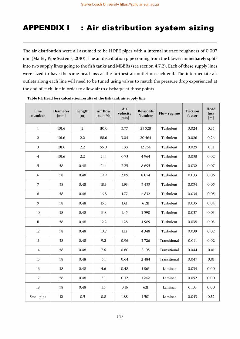
147

: Air distribution system sizing

_________

The air distribution were all assumed to be HDPE pipes with a internal surface roughness of 0.007

mm (Marley Pipe Systems, 2010). The air distribution pipe coming from the blower immediately splits

into two supply lines going to the fish tanks and MBBRs (see section 4.7.2). Each of these supply lines

were sized to have the same head loss at the furthest air outlet on each end. The intermediate air

outlets along each line will need to be tuned using valves to match the pressure drop experienced at

the end of each line in order to allow air to discharge at those points.

Table I-1: Head loss calculation results of the fish tank air supply line

Line number

Diameter [mm]

Length [m]

Air flow [std m3/h]

Air velocity

[m/s]

Reynolds Number

Flow regime Friction

factor

Head loss [m]

1 101.6 2 110.0 3.77 25 528 Turbulent 0.024 0.35

2 101.6 2.2 88.6 3.04 20 564 Turbulent 0.026 0.26

3 101.6 2.2 55.0 1.88 12 764 Turbulent 0.029 0.11

4 101.6 2.2 21.4 0.73 4 964 Turbulent 0.038 0.02

5 58 0.48 21.4 2.25 8 695 Turbulent 0.032 0.07

6 58 0.48 19.9 2.09 8 074 Turbulent 0.033 0.06

7 58 0.48 18.3 1.93 7 453 Turbulent 0.034 0.05

8 58 0.48 16.8 1.77 6 832 Turbulent 0.034 0.05

9 58 0.48 15.3 1.61 6 211 Turbulent 0.035 0.04

10 58 0.48 13.8 1.45 5 590 Turbulent 0.037 0.03

11 58 0.48 12.2 1.28 4 969 Turbulent 0.038 0.03

12 58 0.48 10.7 1.12 4 348 Turbulent 0.039 0.02

13 58 0.48 9.2 0.96 3 726 Transitional 0.041 0.02

14 58 0.48 7.6 0.80 3 105 Transitional 0.044 0.01

15 58 0.48 6.1 0.64 2 484 Transitional 0.047 0.01

16 58 0.48 4.6 0.48 1 863 Laminar 0.034 0.00

17 58 0.48 3.1 0.32 1 242 Laminar 0.052 0.00

18 58 0.48 1.5 0.16 621 Laminar 0.103 0.00

Small pipe 12 0.5 0.8 1.88 1 501 Laminar 0.043 0.32


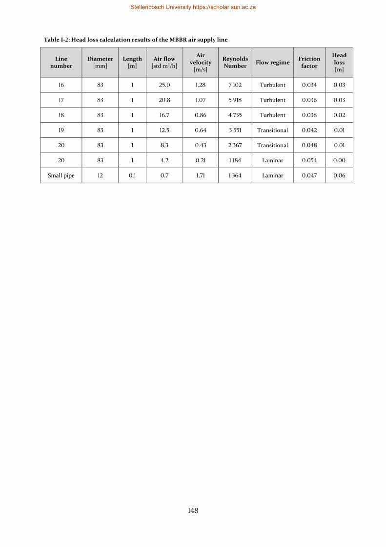
148

Table I-2: Head loss calculation results of the MBBR air supply line

Line number

Diameter [mm]

Length [m]

Air flow [std m3/h]

Air velocity

[m/s]

Reynolds Number

Flow regime Friction

factor

Head loss [m]

16 83 1 25.0 1.28 7 102 Turbulent 0.034 0.03

17 83 1 20.8 1.07 5 918 Turbulent 0.036 0.03

18 83 1 16.7 0.86 4 735 Turbulent 0.038 0.02

19 83 1 12.5 0.64 3 551 Transitional 0.042 0.01

20 83 1 8.3 0.43 2 367 Transitional 0.048 0.01

20 83 1 4.2 0.21 1 184 Laminar 0.054 0.00

Small pipe 12 0.1 0.7 1.71 1 364 Laminar 0.047 0.06


Documents

Design and modeling of an experimental tilapia and African