Embed Size (px)
Citation preview

HAL Id: tel-03311669https://tel.archives-ouvertes.fr/tel-03311669
Submitted on 1 Aug 2021
HAL is a multi-disciplinary open accessarchive for the deposit and dissemination of sci-entific research documents, whether they are pub-lished or not. The documents may come fromteaching and research institutions in France orabroad, or from public or private research centers.
L’archive ouverte pluridisciplinaire HAL, estdestinée au dépôt et à la diffusion de documentsscientifiques de niveau recherche, publiés ou non,émanant des établissements d’enseignement et derecherche français ou étrangers, des laboratoirespublics ou privés.
Design and manufacturing process optimization forprosthesis of the lower limb
Abbass Ballit
To cite this version:Abbass Ballit. Design and manufacturing process optimization for prosthesis of the lower limb.Biomechanics [physics.med-ph]. Université de Technologie de Compiègne, 2020. English. �NNT :2020COMP2589�. �tel-03311669�

Par Abbass BALLIT
Thèse présentée pour l’obtention du grade de Docteur de l’UTC
Design and manufacturing process optimization for prosthesis of the lower limb
Soutenue le 17 novembre 2020 Spécialité : Biomécanique et Bio-ingénierie : Unité de Recherche Biomécanique et Bio-ingénierie (UMR-7338)
D2589

UNIVERSITE DE TECHNOLOGIE
DE COMPIEGNE
PhD Thesis
Biomechanics & Bioengineering
Abbass BALLIT
DESIGN AND MANUFACTURING PROCESS OPTIMIZATION FOR PROSTHESIS OF THE
LOWER LIMB
Defended on 17/11/2020
Jury Members:
DAO Tien-Tuan, Professor, Centrale Lille Institut (Director of the thesis)
MOUGHARBEL Imad, Professor, Ecole de Technologie Supérieure de Montréal (Co-
director of the thesis)
KROMER Valérie, MCF, HDR, Université de Lorraine (Reporter)
MAAROUF Saad, Professor, Ecole de Technologie Supérieure de Montréal (Reporter)
AMINIAM Kamiar, Professor, Polytechnique Fédérale de Lausanne.
HO BA THO Marie-Christine, Professor, UTC-BMBI, Centre de Recherche de Royallieu
Invited Member:
GHAZIRI Hassan, Professor, Beirut Research & Innovation Center.
Spécialité : Biomécanique et Bio-ingénierie


i
Abstract The prosthetic socket, an essential interface element between the patient's stump and prosthetic device,
is most often the place where the degree of prosthetic success is defined. It is the most critical part of
the prosthesis, customized to fit with the unique residual limb of the amputee. Without a proper socket
shape and fit, the prosthesis becomes uncomfortable, or even unusable, and causes pain and skin
issues. The state-of-the-art prosthetic production is still missing universal numerical standards to
design a socket. The current practice is expensive and relies on the manual refinements of the
orthopedic technician, and the fit quality strictly correlates with his skills as well as the subjective
feedback of the patient.
The thesis aims to conduct a deep analysis of an optimal design of the prosthetic socket by studying
and developing an alternative computer-aided design process. This process is fully based on the virtual
model of the patient’s residual limb and relies on the calculation of the socket-stump interaction. A
fast calculation is favorable in this case, that’s why we propose to use the Mass-Spring System (MSS)
instead of the widely used FE method to model the soft tissues of the residual limb. A new
configuration of the MSS model is proposed to respect the non-compressibility property of the soft
tissues by adding non-linear “Corrective Springs”. The numeric model is to be generated from the
scanned model of the stump. For this purpose, we propose a fusion scheme of four RGB-Depth sensors
for a rapid and low-cost scan with error reduction techniques. Finally, the virtual residual limb is used
in the socket designing phase. A parametric design method is proposed and investigated. The design
problem is transformed into a constraint-satisfaction-problem whose constraints are derived from the
inverse calculation of the stump-socket interaction. The inverse approach has been chosen to eliminate
the need for expensive contact formulation. This fact leads to rapid calculations, and consequently,
allows to provide real-time numerical feedback during the designing process. The validation was done
by comparing the results of our system with the output of FE simulations.
The system has been implemented with a user-friendly graphical interface and virtually tested and
numerically validated. This system reduces the limitations of the current practices. However, a lot of
works is still ahead to refine and develop the system and validate it with clinical experiments.
Keywords: lower-limb prosthetic socket, finite element, real-time soft tissues deformation, Mass-
Spring System, 3D scan, computer-aided design

ii

iii
Acknowledgment
With boundless love and appreciation, I would like to extend my heartfelt gratitude and appreciation
to the people who helped me, in any manner, to bring this study into reality.
I am extremely grateful to my supervisors Prof. Tien-Tuan DAO and Prof. Imad MOUGHARBEL for
their consistent support, guidance, motivation, and patience during the running of this project.
Moreover, I would like to thank Prof. Hassan GHAZIRI (Beirut Research and Innovation Center,
Lebanon) for his direction, advices and support. I am sincerely grateful to all of them, I could not have
imagined having better advisors and mentors for my Ph.D. study.
I would also like to give my gratitude to the members of the jury for their interest in my work, and
their desire to examine it.
I would like to thank the Université de Technologie de Compiègne for adopting our project and having
me as a Ph.D. student. I also thank the laboratory BioMécanique et BioIngénierie (BMBI-UMR CNRS
7338) for accepting me as one of its members and facilitating good researching tools during my PhD
period.
Besides, a thank to Mr. Antoine CHAMMAA, the owner of ELIMED orthopedic center, Beirut,
Lebanon, for his time and cooperation that played a big role in the success of the thesis.
Many personnel have contributed to this work. First, I regard Dr. Tan Nhu NGUYEN and Dr. Víctor
ACOSTA SANTAMARÍA whose support as team members at BMBI allowed my studies to go the
extra mile. I would like also to appreciate the support of BRIC members: Dr. Mohammad HUSSEINI,
Dr. Mohammad BAIDOUN, Dr. Ali TAKASH, Mr. Hassan HUSSEINI, and Mr. Mohammad
MINKARA.
I thank my parents, family, and friends for pushing me to achieve my dreams, providing the help I
need with every step, and allowing me to become the person I am today.
Finally, I would like to thank Mrs. Nehmat YOUSSEF, for her emotional support, and the big
sacrifices she made for the sake of my success.
This work was supported by Beirut Research and Innovation Center (BRIC), Beirut, Lebanon.

iv
Pursue your goals even in the face of difficulties,
and convert adversities into opportunities
-Dhirubhai Ambani

v
Table of Contents Abstract ................................................................................................................................................. i
Acknowledgment ................................................................................................................................ iii
Table of Contents ................................................................................................................................ v
List of Figures ...................................................................................................................................... x
List of Tables ..................................................................................................................................... xv
Introduction ................................................................................................................. 1
1.1 Healthcare context ................................................................................................................. 1
1.2 Background ........................................................................................................................... 3
1.2.1 Types and causes of lower limb amputations................................................................ 3
1.2.2 Historical overview of lower-limb prosthetics .............................................................. 6
1.2.3 Prosthetic leg components ............................................................................................. 7
1.2.4 The socket: the most critical part .................................................................................. 8
1.3 Challenges and objective ...................................................................................................... 9
1.4 Organization of the thesis.................................................................................................... 11
State-Of-The-Art ....................................................................................................... 12
2.1 Current socket fabrication practice ..................................................................................... 12
2.1.1 Types and shapes of lower limb prosthetic sockets .................................................... 12
2.1.2 The main rules ............................................................................................................. 14
2.1.3 Pressure-tolerant and pressure-sensitive areas ............................................................ 15
2.1.4 The conventional fabrication method .......................................................................... 16
2.2 Solutions for low-Cost prostheses ....................................................................................... 19
2.3 Review on prosthetic CAD/CAM solutions ........................................................................ 21
2.4 Review on the components of the prosthetic CAD/CAM ................................................... 24
2.4.1 3D scanning of the residual limb ................................................................................ 24
2.4.2 Measurement of biomechanical parameters ................................................................ 25
2.4.3 Stump/socket interaction measurement ....................................................................... 26
2.4.4 Stump/Socket interaction simulation .......................................................................... 29
2.4.5 Socket modeling .......................................................................................................... 30
2.4.6 Rapid prototyping ....................................................................................................... 31

vi
2.5 Discussion ........................................................................................................................... 32
Modeling of the Stump Soft-Tissues and Stump-Socket Interaction .................... 34
3.1 Simulation of deformable objects in biomechanics ............................................................ 34
3.1.1 Finite element method ................................................................................................. 35
3.1.2 Position-based dynamics ............................................................................................. 35
3.1.3 Meshless deformations ................................................................................................ 35
3.1.4 Mass-springs-system ................................................................................................... 36
3.2 The proposed model (MSS-CS) .......................................................................................... 37
3.2.1 System configuration .................................................................................................. 37
3.2.2 Parameters identification ............................................................................................. 37
3.2.3 Volume conservation .................................................................................................. 39
3.2.4 Simulation algorithm ................................................................................................... 40
3.3 Interaction with rigid body .................................................................................................. 41
3.3.1 Socket modeling .......................................................................................................... 41
3.3.2 Contact modeling ........................................................................................................ 41
Development of simulation environment ................................................................................ 45
3.4.................................................................................................................................................... 45
3.4.1 Implementation ........................................................................................................... 45
3.4.2 The Stump’s Model ..................................................................................................... 46
3.4.3 Simulation Stability ..................................................................................................... 47
3.5 Accuracy analysis ............................................................................................................... 48
3.6 Results ................................................................................................................................. 51
3.7 Discussions.......................................................................................................................... 55
Rapid Low-Cost 3D Scan of the Stump ................................................................... 57
4.1 Microsoft Kinect v2 RGB-Depth sensor ............................................................................. 57
1. General overview ................................................................................................................ 57
4.1.1 Point-cloud generation ................................................................................................ 58
4.2 Kinect V2 accuracy ............................................................................................................. 59
4.2.1 Imprecision of the Kinect v2 sensor ............................................................................ 59

vii
4.2.2 Accuracy analysis........................................................................................................ 59
4.2.3 Error compensation technique ..................................................................................... 61
4.2.4 The learning database of the error Compensation technique ...................................... 62
4.3 The 3D-scanning platform .................................................................................................. 64
4.3.1 System architecture ..................................................................................................... 64
4.3.2 Multi-set registration problem ..................................................................................... 66
4.3.3 3D reconstruction ........................................................................................................ 68
4.4 Application .......................................................................................................................... 69
4.4.1 Technical implementation ........................................................................................... 69
4.4.2 Accuracy evaluation .................................................................................................... 70
4.5 Results ................................................................................................................................. 70
4.5.1 Accuracy of the error compensation strategy .............................................................. 70
4.5.2 Speed of the scanning process ..................................................................................... 75
4.5.3 Accuracy of the multiple point cloud registration process .......................................... 75
4.6 Discussions.......................................................................................................................... 76
Parametric Digital Design of the Prosthetic Socket ............................................... 79
5.1 Computer-aided parametric socket design workflow.......................................................... 79
5.2 Inverse approach for stump-socket interaction ................................................................... 80
5.2.1 Theoretical basis ......................................................................................................... 80
5.2.2 Inverse approach ......................................................................................................... 82
5.3 Interactive parametric design .............................................................................................. 84
5.4 Application and accuracy evaluation .................................................................................. 88
5.5 Computational results ......................................................................................................... 90
5.5.1 Socket design outcomes .............................................................................................. 90
5.5.2 Evaluation with FE Simulations outcomes ................................................................. 91
5.6 Discussion ........................................................................................................................... 94
General Discussions .................................................................................................. 99
6.1 Thesis objective ................................................................................................................... 99
6.2 The achieved system ........................................................................................................... 99

viii
6.3 Main contributions ............................................................................................................ 103
6.3.1 MSS-CS model for fast soft-tissues deformation ...................................................... 103
6.3.2 Error compensation strategy for the Kinect v2 sensor .............................................. 103
6.3.3 OpenMKS 3D-scanning platform ............................................................................. 103
6.3.4 Constraint satisfaction approach for a numerical socket design with real-time
feedback 104
6.4 Limitations ........................................................................................................................ 104
Conclusions & Perspectives .................................................................................... 107
7.1 Summary of the thesis ....................................................................................................... 107
7.2 General perspectives ......................................................................................................... 108
Publications ..................................................................................................................................... 110
National Conference ..................................................................................................................... 110
Journal Articles ............................................................................................................................. 110
References ........................................................................................................................................ 111
Appendix: Abaqus for Finite Element Analysis ........................................................................... 138
A.1. Overview on Finite Element Analysis .................................................................................. 138
A.1.1. What is FEA? ................................................................................................................. 138
A.1.2. Domain and Boundary Conditions ................................................................................. 139
A.1.3. Strong and Weak Forms of Boundary Problem ............................................................. 139
A.2. Soft-Tissue FE Modeling ...................................................................................................... 143
A.2.1. Mooney-Rivlin Model .................................................................................................... 145
A.2.2. Yeoh Model .................................................................................................................... 145
A.2.3. Neo-Hookean Model ...................................................................................................... 145
A.2.4. Odgen Model .................................................................................................................. 146
A.2.5. Humphrey Model ........................................................................................................... 147
A.2.6. Veronda-Westmann Model ............................................................................................ 147
A.3. Introduction to Abaqus .......................................................................................................... 148
A.4. FEA Solution Sequence ........................................................................................................ 149
A.5. System Modeling Using Abaqus ........................................................................................... 149

ix
A.5.1. Geometries ..................................................................................................................... 149
A.5.2. Meshing .......................................................................................................................... 150
A.5.3. Materials ......................................................................................................................... 151
A.5.4. Interactions ..................................................................................................................... 152
A.5.5. Boundary Conditions and Constraints ............................................................................ 154
A.5.6. Simulation Steps ............................................................................................................. 155

x
List of Figures Figure 1. typical lower limb prosthetic device ..................................................................................... 7
Figure 2. The workflow of a typical prosthetic socket CAD/CAM system ......................................... 10
Figure 3. different anatomical positions typically used to describe a socket ..................................... 12
Figure 4. lateral and anterior view of the different configurations of the PTB design: PTB-SC (a),
PTB-SCSO (b), PTK / KBM (c). The red arrow shows the patellar bar where the load is
mainly applied to the patellar tendon. .............................................................................. 13
Figure 5. above-knee prosthetic socket designs ................................................................................. 14
Figure 6. (a) pressure-sensitive and pressure-tolerant areas for the transtibial stump. (b) pressure-
sensitive and pressure-tolerant areas for the transfemoral stump ................................... 15
Figure 7. The steps of the conventional prosthetic socket fabrication method .................................. 16
Figure 8. Examples of existing low-cost lower limb prosthetic solution: (a) below-knee prosthesis
without forefoot [56]; (b) PCAST prosthetic socket [57]; (c) “Jaipur Foot” workshop;
(d) exo-prosthetic limb; (e) adjustable low-cost prosthesis [61]; (f) lower limb prosthesis
fabricated from plastic waste [62] .................................................................................... 19
Figure 9. Literature examples of the proposed prosthetic socket CAD/CAM systems [69-73] ......... 22
Figure 10. Examples from the literature of machine-learning-based socket design methods [77-79]
.......................................................................................................................................... 23
Figure 11. Examples from the literature of the used 3D-scanning techniques [76, 97, 103, 110] .... 24
Figure 12. Examples of limb measurement devices: (a) Active biological indenter mounted in a
static base [125]; (b) FitSocket device [59] ..................................................................... 26
Figure 13. Examples of pressure sensors: (a) traditional strain gauge [134]; (b) three common
types of FSRs: Interlink, LuSense, and FlexiForce [141] ................................................ 27
Figure 14. Transducer mounting techniques: (a) transducer mounted on socket wall through a
drilled hole and the piston extended to be in direct contact with residual limb skin; (b)
the same mounting technique with a slight difference that the piston is flush with the
inner socket face and does not penetrate the liner; (c) transducer inserted inside
prosthetic socket; and (d) transducer embedded in the socket wall [163]. ...................... 28
Figure 15. Examples from the literature of FE simulations of the stump-socket interaction
[178.179,181,182] ............................................................................................................ 30
Figure 16. The elastic connection between 2 punctual masses in MSS, with initial length L0, stiffness
k, and damping coefficient c ............................................................................................. 36
Figure 17. (a) Hexahedral MSS model and (b) hexahedral element with the 28 possible connections:
12 edge connections in blue, 12 faces diagonals in red, and 4 internal diagonals in green
.......................................................................................................................................... 37

xi
Figure 18. Cubical elastic object subject to normal compression pressure: (a) Compressible
material modeled using MSS without corrective springs. (b) Uncompressible material
modeled using MSS with corrective springs performing horizontal expansion to conserve
its volume .......................................................................................................................... 40
Figure 19. The 3D triangular surface of a transtibial prosthetic socket: (a) shaded view; (b)
wireframe view .................................................................................................................. 41
Figure 20. Schematic representation of the collision taking place between the point Pi and the
triangle Tj .......................................................................................................................... 42
Figure 21. collision detected between the point Pi and the triangle Tj ............................................... 42
Figure 22. (a) Forces applied to the point are toward the triangle, so the contact force exists. (b)
The forces applied to the point are not toward the triangle, so no contact force is
considered ......................................................................................................................... 44
Figure 23. The graphical user interface of the developed simulation environment ........................... 46
Figure 24. the reconstruction process of the stump's model from CT images .................................... 47
Figure 25. The stability regions for backward (left) and forward (right) [240] ................................ 48
Figure 26. Study cases for the accuracy analysis: (a) compression of the pink elastic cube due to the
weight of the blue rigid box; (b) simulation of the socket donning process ..................... 49
Figure 27. Optimal meshed stump model used in socket donning simulation .................................... 50
Figure 28. Contact pressure on the upper surface of the elastic cube as a function of the rigid box
weight ................................................................................................................................ 51
Figure 29. Displacement ratio of elastic cube upper surface as a function of the rigid box weight .. 51
Figure 30. The volume of the elastic object as a function of applied weight ................................... 52
Figure 31. Contact pressure distribution on the stump-socket interface from both MSS-CS and FE
simulations at the end of the socket donning process ....................................................... 53
Figure 32. the two point-sets chosen for quantitative evaluation ....................................................... 54
Figure 33. Contact pressure distribution on the vertical points set ................................................... 54
Figure 34. Contact pressure distribution on the horizontal points set ............................................... 54
Figure 35. The Kinect V2 sensor front with cameras and emitter positions [262] ............................ 57
Figure 36. A0 chessboard used for the quantification of the Kinect's imprecision (a) and dimensions
used to calculate the errors assigned to the point Pci,j within the A0 chessboard (b). ...... 60
Figure 37. Absolute error distribution for all frames within the A0 chessboard taken from different
angles (3°, -26°, and 37°) ................................................................................................. 61
Figure 38. (a) example of a random chessboard frame received from Kinect sensor and (b)
chessboard dimensions in the domain ......................................................................... 63

xii
Figure 39. The proposed 3D scanning platform with four RGB-Depth Kinects v2 cameras and
mobile supports (a) and the physical dimension of the space of interest within the 3D
scanning system (b). .......................................................................................................... 65
Figure 40. 3D scanning system workflow from data fusion to 3D surface reconstruction: (a) the four
acquired point-clouds; (b) filtered point-clouds; (c) aligned point-clouds using multi-set
registration method; (d) reconstructed 3D surface of the limb ........................................ 66
Figure 41. Illustration of outlier removal from the point cloud of a scanned white tube (a) and the
rigid multi-set registration process for four point-clouds (b). .......................................... 66
Figure 42. 3D reconstruction problem: (a) using Poisson or scale-space; (b) the process using both
Poisson and scale-space algorithm .................................................................................. 68
Figure 43. Graphical User Interface of OpenMKS ............................................................................ 69
Figure 44. (a) The calibration box, (b) the three cylindrical test objects .......................................... 70
Figure 45. Dimensions error patterns in the horizontal and vertical planes for the three tested
chessboard frames without and with error compensation for the Kinect sensor K1 (AE:
Absolute Error). ................................................................................................................ 71
Figure 46. Dimensions error patterns in the horizontal and vertical planes for the three tested
chessboard frames without and with error compensation for the Kinect sensor K2 (AE:
Absolute Error). ................................................................................................................ 71
Figure 47. Dimensions error patterns in the horizontal and vertical planes for the three tested
chessboard frames without and with error compensation for the Kinect sensor K3 (AE:
Absolute Error). ................................................................................................................ 72
Figure 48. Dimensions error patterns in the horizontal and vertical planes for the three tested
chessboard frames without and with error compensation for the Kinect sensor K4 (AE:
Absolute Error). ................................................................................................................ 72
Figure 49. Dimensions error patterns for the three tubes reconstructed using sensor fusion without
and with applying the error compensation technique. ...................................................... 74
Figure 50. Average timeline of the full scanning process. ................................................................. 75
Figure 51. steps and visual reconstruction outcome of the multi-set registration. ............................ 75
Figure 52. The proposed computer-aided parametric socket design workflow to automatically
generate a patient-specific virtual socket prototype. ........................................................ 80
Figure 53. illustrations of the applied loads by the socket to the stump during the standing up
posture (a) and the force components applied to a single node of the stump’s surface (b).
.......................................................................................................................................... 81
Figure 54. The cylindrical coordinate system for a transtibial residual limb model. ........................ 85
Figure 55. The socket design system: (a) the GUI of the system; (b) interactive elements to apply the
parametric functions; (c) list of applied parametric functions and parameters’ tuning

xiii
tools; (d) the radar chart displaying the real-time feedback (the green line represents the
normalized value of each variable and the yellow circle represents the target values). .. 87
Figure 56. the pain-threshold distribution assigned to the stump's surface: (a) front-lateral view, (b)
back-medial view. ............................................................................................................. 88
Figure 57. The initial state of the FE simulation of the stump-socket interaction using Abaqus
software (a), and the three paths chosen for the quantitative evaluation: (b) the front-
line, (c) the back-line, (d) the circumference. ................................................................... 89
Figure 58. Illustration of interactive steps of the parametric socket design process applied to the
CT-based stump model...................................................................................................... 90
Figure 59. the final applied pressures, the deformations of the stump, and the generated socket for
the 60Kg weighted patient, with both 100Kpa and 200 KPa soft tissues Young's modulus
(E) ..................................................................................................................................... 91
Figure 60. the final applied pressures, the deformations of the stump, and the generated socket for
the 80Kg weighted patient, with both 100Kpa and 200 KPa soft tissues’ Young's modulus
(E) ..................................................................................................................................... 91
Figure 61. The contact pressure distributions resulted from the FE simulations. (a) M=60Kg and
E=100KPa, (b) M=80Kg and E=200KPa, (c) M=80Kg and E=100KPa, (d) M=80Kg
and E=200KPa. ................................................................................................................ 92
Figure 62. Contact pressure resulted from the FE simulation compared to the applied pressures and
the paint-threshold for the front-line point-set, for 60 Kg patient (a) and 80Kg patient
(b). ..................................................................................................................................... 93
Figure 63. Contact pressure resulted from the FE simulation compared to the applied pressures and
the paint-threshold threshold for the back-line point-set, for 60 Kg patient (a) and 80Kg
patient (b). ......................................................................................................................... 93
Figure 64. Contact pressure resulted from the FE simulation compared to the applied pressures and
the paint-threshold for the circumference point-set, for 60 Kg patient (a) and 80Kg
patient (b). ......................................................................................................................... 94
Figure 65. the diagram of the achieved system ................................................................................ 100
Figure 66. Example of a problem in linear stress analysis or linear elasticity ................................ 139
Figure 67. (a) prosthetic socket imported as a part, (b) lower residual limb imported as a part, (c)
the assembly of the two parts .......................................................................................... 150
Figure 68. Examples of the three meshing techniques: structural mesh (a), swept mesh (b), free mesh
(c). (Digital Image, ABAQUS/CAE User’s Manual v6.6. url :
https://classes.engineering.wustl.edu/2009/spring/mase5513/abaqus/docs/v6.6/books/usi/
default.htm?startat=pt03ch17s03s03.html ) ................................................................... 151

xiv
Figure 69. Examples of material properties settings in Abaqus: linear elastic model (a), and
hyperelastic models (b) ................................................................................................... 152
Figure 70. Mechanical loads in ABAQUS/CAE ............................................................................... 154
Figure 71. Examples of boundary conditions (constraints) provided in ABAQUS/CAE ................. 155

xv
List of Tables Table 1. Parameters of the FE simulation performed by Abaqus ....................................................... 50
Table 2. Iterative rigid multi-set registration algorithm for four point-clouds captured from four
Kinects K1, K2, K3, and K4. ............................................................................................. 67
Table 3. Dimensions’ errors of the edge points of the three tested chessboards in horizontal and
vertical planes without and with error compensation for all Kinect sensors (K1, K2, K3,
AND K4) ........................................................................................................................... 73
Table 4. Summary of the registration errors for different registration schemes ................................ 76
Table 5. The key-functions used to build the parametric functions of the local pressure distribution.
.......................................................................................................................................... 85
Table 6. The parametric functions of the local force distributions. .................................................... 86
Table 7. Used values of the pain-threshold pressures in the key zones of the stump model. .............. 88
Table 8. Comparison of the proposed approach with the available socket CAD systems .................. 95

1
Introduction
1.1 Healthcare context
Almost all of us were naturally born with those two weight-bearing and locomotive biological devices, the
lower limbs, and when we first started walking, it was one of the greatest moments for us and freaking
hilarious moments for the parents. Whereas it required a great job to switch from crawling to walking, the
latter has become now a very simple daily task that we perform intuitively. Not just standing and walking,
but even running and jumping…etc. are very easy works that we enjoy doing. But as easy and simple as
they sound, many people are deprived of the “luxury” of performing them because they’ve lost one or both
their lower limbs.
Limb loss, also known as an amputation, is a major physical and psychologically overwhelming event that
can happen to a person. Amputation represents an irreversible surgical option which may result in
physically challenged and bodily disfigurement. The amputations occur everywhere in the world, either in
developed or developing countries, and the causes of amputation are many. The most common reason is
poor blood circulation because of the damage or narrowing of the arteries, called peripheral arterial disease.
Diabetes can be one of the causes of this vascular issue. Without adequate blood flow, the body's cells
cannot get the oxygen and nutrients they need from the bloodstream. As a result, the affected tissue begins
to die and infection may set in. Sometimes, a bad infection never heals and might cause gangrene. Gangrene
and foot ulcers that do not get better with treatment can lead to an amputation to prevent the bad infection
from spreading to the rest of the patient’s body. Other causes for amputation may include a cancerous tumor
in the bone or muscle of the limb, thickening of nerve tissue (called a neuroma), frostbite, and severe injury
(from a vehicle accident or serious burn, for example) … etc. Besides, there are, of course, the victims of
the conflicts in war and post-war zones where the greatest number of amputations result from the fighting
and landmine explosions.
Limb loss is much more common than many people realize. Despite advances in medicine and
biomechanics, amputations continue to be a large and rapidly growing problem worldwide that impacts
millions of individuals. In the United States, nearly 2 million people are living with limb loss, and the
number will nearly double by the year 2050 [1] since approximately 185,000 amputations occur all over
the states each year [2]. Globally, epidemiological reports during the last decade indicated that over 1
million amputations were being performed on people with diabetes each year [3], which means that a leg

2
is lost to diabetes somewhere in the world every 30 seconds. And of these people, up to 55% will require
amputation of the contralateral leg within 2‐3 years [4].
Amputation of the limbs has been reported to a be significantly stressful event for an individual [5-6], and
it has severe psychological and emotional effects on the amputee that may result in a poor quality of life
[7]. Many researches in the field reported that traumatic loss of a limb is typically equated with loss of
spouse [8], loss of one's perception of wholeness [9], symbolic castration, and even death [10-11].
Immediate reactions to the prospect of amputation vary and depend on whether the amputation was planned,
occurred within the context of a chronic medical illness, or was necessitated by the sudden onset of infection
or trauma. The context for amputation affects the psychological sequelae during the rehabilitation phase as
well. When there is time to think about impending loss, classic stages of grief may be experienced [12].
Among these stages are denial (often manifest as a refusal to engage in discussion or to ask basic questions
about the planned procedure), anger (which may be directed toward the medical team, with expressions of
being “cheated” or “tricked” into agreeing to an amputation), bargaining (by attempting to forestall the
surgery or to delay it indefinitely for a myriad of reasons such as “I'm too tired, I don't want to go through
with any major surgery”), depression (taking the form of “learned helplessness,” feelings of passivity, and
being overwhelmed), and acceptance (which may not be reached until the patient is well into the
rehabilitation process) [13].
Despite the variety of the amputee’s reactions toward the amputation fact, the current most important path
for them is the one that allows them to maintain their independence and livelihood - and that starts with
walking. Thankfully, we finally have advanced prosthetic devices that allow the amputees to not only walk
again but run and even compete professionally with individuals who have biologically standard limbs. With
the advancement in technology, prosthetic limbs have reached a new level of quality and function. Lower
limb prosthetics have moved from hooks and pegs to bionic legs made with microprocessor knees that allow
amputees to walk up and down stairs with minimal struggle. Unfortunately, these advancements come with
a hefty price tag and prosthetics can’t be accessed by everyone in need. In developed countries, according
to a market analysis [14], a simple lower limb prosthesis with no sophisticated technology that allows its
user to simply stand and walk on level ground costs between $5,000 and $7,000. On the other hand, a
$10,000 device will allow the person to become a "community walker" able to go up and down stairs and
to traverse uneven terrain. Whereas to walk and run at a level nearly indistinguishable from someone with
two legs, the amputee will need a prosthetic leg in the $12,000 to $15,000 price range. Add this to the
physical therapy costs that go with learning how to use the device, the 3-5 years life span of most prosthetic
limbs, and other medical issues associated with the amputation, and the cost totals to more than typical
college tuition fees. The lifetime per patient cost calculations for amputees suggest dollar amounts ranging
between $800,000 and $1.81 million [15-16], which is 1.4- to 3.2-times more than the lifetime medical cost
for the average person (US$562,880) [17]. While many institutions are striving to improve the lives of
3
amputees through research and technology, the target market for these discoveries will remain small if the
price tags are not lowered.
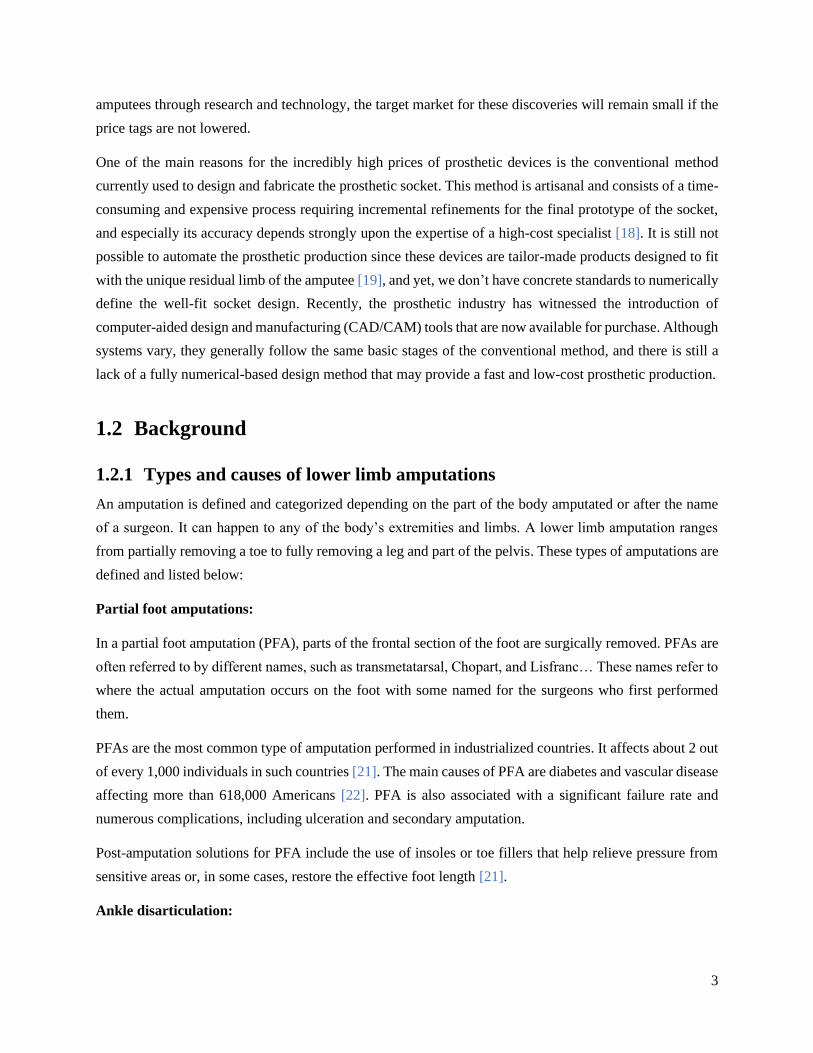
One of the main reasons for the incredibly high prices of prosthetic devices is the conventional method
currently used to design and fabricate the prosthetic socket. This method is artisanal and consists of a time-
consuming and expensive process requiring incremental refinements for the final prototype of the socket,
and especially its accuracy depends strongly upon the expertise of a high-cost specialist [18]. It is still not
possible to automate the prosthetic production since these devices are tailor-made products designed to fit
with the unique residual limb of the amputee [19], and yet, we don’t have concrete standards to numerically
define the well-fit socket design. Recently, the prosthetic industry has witnessed the introduction of
computer-aided design and manufacturing (CAD/CAM) tools that are now available for purchase. Although
systems vary, they generally follow the same basic stages of the conventional method, and there is still a
lack of a fully numerical-based design method that may provide a fast and low-cost prosthetic production.
1.2 Background
1.2.1 Types and causes of lower limb amputations
An amputation is defined and categorized depending on the part of the body amputated or after the name
of a surgeon. It can happen to any of the body’s extremities and limbs. A lower limb amputation ranges
from partially removing a toe to fully removing a leg and part of the pelvis. These types of amputations are
defined and listed below:
Partial foot amputations:
In a partial foot amputation (PFA), parts of the frontal section of the foot are surgically removed. PFAs are
often referred to by different names, such as transmetatarsal, Chopart, and Lisfranc… These names refer to
where the actual amputation occurs on the foot with some named for the surgeons who first performed
them.
PFAs are the most common type of amputation performed in industrialized countries. It affects about 2 out
of every 1,000 individuals in such countries [21]. The main causes of PFA are diabetes and vascular disease
affecting more than 618,000 Americans [22]. PFA is also associated with a significant failure rate and
numerous complications, including ulceration and secondary amputation.
Post-amputation solutions for PFA include the use of insoles or toe fillers that help relieve pressure from
sensitive areas or, in some cases, restore the effective foot length [21].
Ankle disarticulation:

4
The ankle disarticulation is a disarticulation at the tibiotalar joint with resection of the malleoli. The heel
pad is used to cover the end of the tibia.
This kind of amputation is also known as Syme’s amputation technique or Syme’s ankle disarticulation. It
is named that way after “James Syme” who suggested this technique and first recorded it in the adult in
1843 [20]. The traditional Syme amputation is a 1-stage procedure. Later, a 2-stage procedure was designed,
with the first stage used for debridement in case of infection with only loose closure and the second stage
for trimming of the malleoli and revision of the skin flap [23].
Syme ankle disarticulation is an amputation level that minimizes disability and preserves function. It
maintains an end-bearing and durable residual limb and provides better proprioception in the prosthesis
because of the preservation of the heel pad [24-25]. But on the other hand, Syme’s amputation has several
disadvantages that avoided surgeons performing this amputation level such as the perceived high risk for
wound failure, wound infection, or migration of the heel pad, which makes prosthesis use difficult [25-26].
Other disadvantages include that it is harder to build an appealing cosmetic prosthesis, and the options
available for a prosthetic foot are limited [27].
Transfemoral:
Transfemoral amputations, also known as above-knee amputations (AKA), involve removing the leg from
the body by cutting the lower-limb above the knee joint through both the thigh tissue and femoral bone.
Above-the-knee amputations may be necessary for many reasons. These can include trauma to the lower
leg, which results in a non-viable leg at or near the level of the knee. Below-the-knee amputation may
adequately address a more distal injury. Many studies have attempted to create algorithms to help
physicians decide when to reconstruct versus amputate. One of these is the Mangled Extremity Severity
Score (MESS), which takes into account skeletal/soft tissue injury, limb ischemia, shock, and patient age
[28]. Other indications include infection which has compromised the entire lower leg and is unresectable.
Etiologies may include non-healing diabetic wounds, necrotizing fasciitis, or cases of immunocompromised
patients. Tumors that are unresectable or whose resection would render the distal aspect of the limb non-
usable are yet another indication for this procedure. Vascular compromise, whether from injury or disease,
which cannot be corrected, can also necessitate an AKA. Additionally, congenital disabilities that render a
limb non-usable can indicate the need for this amputation. Individuals who have suffered an above-knee
amputation have the possibility of regaining mobility and walking again by using a prosthesis [29].
Transtibial:
Transtibial amputations, also known as below-knee amputations (BKA), involve cutting the lower limb
below the knee joint. Usually, the surgeon will prefer to perform a BKA over an AKA, if possible, to
preserve a healthy knee joint which makes the BKA have better rehabilitation and functional outcomes
[30]. In fact, knee joints are beneficial to balance, as well as maintaining the ability to lift and lower oneself.

5
Knees also allow us to slow down, walk on stairs and slopes, and push forward. A prosthetic knee provides
the bending ability of a knee, but not the power, since a prosthetic knee is basically a swinging hinge.
There are two major bones in the lower leg that the surgeon considers when performing a transtibial
amputation. The larger of the two leg’s bones is the tibia, the smaller is the fibula. These bones are joined
at the top and bottom by joints at the knee and ankle. When these bones are surgically divided in transtibial
amputation, they maintain their joining near the knee, but not below.
A below-the-knee amputation is performed when a lower part of the leg becomes severely injured or
develops a life-threatening infection. Other reasons include chronic pain, birth defects, tumors, and non-
healing ulcers. The decision to amputate involves many factors and is done after a thorough discussion
between the patient and the orthopedic surgeon. One of these factors is the urgent cases where source control
of necrotizing infections or hemorrhagic injuries becomes more important than limb preservation. These
operations are executed when the patient’s life is threatened, and may sometimes, require bedside operation
if there is insufficient time to reach the operative suite.
Transtibial amputations are the most common amputations worldwide. It represents 71% of dysvascular
amputations [31]. Patients with a BKA have the option to use an artificial leg, also called a transtibial
prosthesis that can allow them to walk and restore mobility [27].
Knee disarticulation:
The Knee Disarticulation (KD) style of amputation is performed by amputating the limb between the bones
in the knee joint instead of cutting through either bone. This kind of amputation is most commonly done
after tumor resection or when an individual has suffered severe trauma.
KD represents less than 2% of the annual amputations performed in lower limbs in the United States [32].
Similar to below-knee amputees, a patient with a KD amputation has the possibility of regaining mobility
with the use of a custom-made prosthesis [29]. Several advantages of the knee disarticulation include a
large end surface covered by skin and soft tissues that are naturally suited for weight-bearing, a long lever
arm controlled by strong muscles, and increased stability of the patient’s prosthesis.
despite numerous advantages, KDs are rarely performed because of the anticipated KD prosthesis fitting
problems that include the positioning of the knee joint distally from the KD socket [33]. Another main
reason disadvantage of this kind of amputation is cosmetic.
Hip Disarticulation and Hemipelvectomy:
Hip disarticulation and hemipelvectomy, also known as trans pelvic amputation, are types of amputation
that leave the amputee with the loss of three joints: the hip, the knee, and the ankle. A hip disarticulation is

6
the amputation of the entire lower limb at the hip level, whereas a hemipelvectomy is the amputation of the
entire lower limb, plus a portion of the pelvic bone.
Hip disarticulation usually occurs due to trauma, tumors, and severe infections, but can be used to treat
vascular disease or be the result of complications that arise from diabetes.
A hemipelvectomy is a high-level pelvic amputation. It consists of removing half of the pelvis to treat
localized tumors, and, rarely, cancer that has metastasized on the area. Examples of cancers that can require
hemipelvectomies are sarcomas like Ewing's Sarcoma, osteosarcoma, or chondrosarcoma.
There are two types of Hemipelvectomy. The first type is the external one, also known as hindquarter
amputation which consists of the amputation of the whole leg plus the pelvis on that side. The second type
is the internal Hemipelvectomy, which is the removal of the pelvis on the one side, but without removal of
the leg.
Individuals who have undergone an internal hemipelvectomy amputation and lost their legs can regain
mobility and walk again with the use of a prosthesis [34]. Whereas for hip disarticulation, the use of a new
prosthesis is acceptable and can provide mobility to the amputee with intensive physical therapy and
psychological rehabilitation [35].
Van Nes rotationplasty:
Rotationplasty, commonly known as a Van Nes rotation or Borggreve rotation, is a type of autograft
wherein a portion of a limb is removed, while the remaining limb below the involved portion is rotated and
reattached. This procedure is used when a portion of an extremity is injured or involved with a disease, such
as cancer [36].
1.2.2 Historical overview of lower-limb prosthetics
A prosthesis is an artificial device that replaces a missing body part. It is also commonly known as an
artificial limb or simply a "prosthetic," and is an externally applied device that is designed to make the loss
of a limb less drastic for everyday life and to improve quality of life for those who have experienced
amputations. Lower limb prosthesis, or simply prosthetic leg, is intended to help patients to regain their
mobility and independence.
The medical world has witnessed a very big advancement in prosthetic technologies, for instance, we now
have advanced technologies that can give us access to robotic limbs. But it hasn’t always been this way,
though, and in the past, it was much more difficult for people to adjust to life after losing a limb than it is
today.

7
The very first documented use of the prosthesis in human history was reported in 2000 [37] when research
pathologists discovered an Egyptian mummy with a prosthetic toe made of wood and leather. The Greeks
also left evidence of using wooden feet to replace the lost biological ones.
In the middle ages, peg legs and hand hooks were common for those who could afford to have them fitted.
An increasing number of tradesmen crafted prosthetics during this time. For example, those who made
watches often used gears and springs to give limbs more detailed functionality. During the Renaissance,
Copper, iron, steel, and wood were the most common materials used for prosthetics.
The prosthetic devices were still very heavy until the post-World War II period, where most limbs were
made of a combination of wood and leather. Whereas wood is heavy, leather can be difficult to keep clean,
especially since it absorbs perspiration. Thereafter, in the second half of the 20th century, plastics,
polycarbonates, resins, and laminates were introduced as light, easy-to-clean alternatives to wood and
leather models. Lightweight materials such as carbon fiber were also introduced.
Today’s prosthetic limbs are much lighter and less cumbersome than those of the past. They’re typically
made of plastic, aluminum, and composite materials that provide amputees with function and mobility.
Motorized hand prosthetics controlled by sensors and microprocessors have also emerged. Thanks to new
technologies and the improvement of materials, prosthetics have come a long way since the first known
wooden toe. Developments in technologies such as robotics, brain-computer interfaces, and 3D-printing
have the potential to lead to future advancements in the field of prosthetics.
1.2.3 Prosthetic leg components
Beside the adapters and other connecting accessories, a prosthetic leg typically consists of the following
three main components: prosthetic foot, pylon, and socket (Figure 1). For the transfemoral (above-knee)
prosthetic leg, a knee unit is also introduced [38].
Figure 1. typical lower limb prosthetic device

8
The prosthetic foot:
A prosthetic foot is the lowest part of the prosthetic leg. It should ideally imitate the function of a real foot
as closely as possible by providing a safe platform, handling differences in terrain, and allowing the user to
walk in a natural, symmetrical way. It’s the main prosthetic component responsible for absorbing the shock
generated by the impact on the ground due to the absence of muscles from the amputated limb, and it should
also help the user to walk more easily by returning the energy generated by the impact of walking.
The pylon:
Also known as “shank”, it is the skeleton of a prosthetic limb. It has traditionally been formed of metal
rods, as it must provide structural support. Recently, however, the pylons have been formed from lighter
carbon-fiber composites. Sometimes the pylons are enclosed by a cover, which is typically made from a
foam-like material, in order to mimic the real leg shape.
The socket:
The socket is the part of the prosthetic device that connects to the patient's residual limb. Because it
transmits forces from the prosthetic limb to the patient's body, the socket must be meticulously fitted to
avoid causing irritation or damage to the skin or underlying tissues. Typically, a soft liner is situated within
the interior of the socket, playing a key role in suspending the socket from the residual limb and as a
protective barrier between the skin and the socket.
Sockets are often part of the overall suspension mechanisms securing the prosthetic limb to the residual
limb. Many suspension techniques are currently used in the prosthetic limbs including the harness system
(belts or sleeves are used to attach the prosthetic device), mechanical lock (by the incorporation of a pin
attached at the end of a liner which engages into a lock in the socket), suction suspension (such as the use
of sealed-in liner and air expulsion valve) and anatomical suspension (when the contours of the prosthetic
socket capture and hold onto the contours of the patient’s body).
1.2.4 The socket: the most critical part
The socket is the interface between the prosthetic device and the amputee’s stump. During static and
dynamic situations, forces and moments are transferred from the socket to the skeletal structures via soft
tissues. Knowing that the residual limb soft tissues are not physiologically designed to tolerate these forces
and moments, the challenge is to create a socket with an interface pressure that has a stiff coupling with the
bony skeleton and, at the same time, does not overstress the soft tissues [39]. Thus, the socket is the primary
and critical part that determines the level of comfortability of the prosthesis, and a good and comfortable
well-fit socket is required to ensure a positive outcome is reached in an amputee’s rehabilitation [40].
9
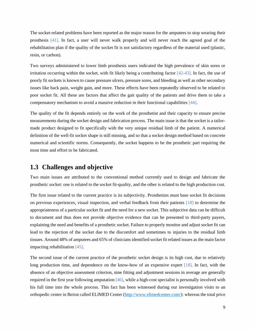
The socket-related problems have been reported as the major reason for the amputees to stop wearing their
prosthesis [41]. In fact, a user will never walk properly and will never reach the agreed goal of the
rehabilitation plan if the quality of the socket fit is not satisfactory regardless of the material used (plastic,
resin, or carbon).
Two surveys administered to lower limb prosthesis users indicated the high prevalence of skin sores or
irritation occurring within the socket, with fit likely being a contributing factor [42-43]. In fact, the use of
poorly fit sockets is known to cause pressure ulcers, pressure sores, and bleeding as well as other secondary
issues like back pain, weight gain, and more. These effects have been repeatedly observed to be related to
poor socket fit. All these are factors that affect the gait quality of the patients and drive them to take a
compensatory mechanism to avoid a massive reduction in their functional capabilities [44].
The quality of the fit depends entirely on the work of the prosthetist and their capacity to ensure precise
measurements during the socket design and fabrication process. The main issue is that the socket is a tailor-
made product designed to fit specifically with the very unique residual limb of the patient. A numerical
definition of the well-fit socket shape is still missing, and so that a socket design method based on concrete
numerical and scientific norms. Consequently, the socket happens to be the prosthetic part requiring the
most time and effort to be fabricated.
1.3 Challenges and objective
Two main issues are attributed to the conventional method currently used to design and fabricate the
prosthetic socket: one is related to the socket fit-quality, and the other is related to the high production cost.
The first issue related to the current practice is its subjectivity. Prosthetists must base socket fit decisions
on previous experiences, visual inspection, and verbal feedback from their patients [18] to determine the
appropriateness of a particular socket fit and the need for a new socket. This subjective data can be difficult
to document and thus does not provide objective evidence that can be presented to third-party payers,
explaining the need and benefits of a prosthetic socket. Failure to properly monitor and adjust socket fit can
lead to the rejection of the socket due to the discomfort and sometimes to injuries to the residual limb
tissues. Around 48% of amputees and 65% of clinicians identified socket fit related issues as the main factor
impacting rehabilitation [45].
The second issue of the current practice of the prosthetic socket design is its high cost, due to relatively
long production time, and dependence on the know-how of an expensive expert [18]. In fact, with the
absence of an objective assessment criterion, nine fitting and adjustment sessions in average are generally
required in the first year following amputation [46], while a high-cost specialist is personally involved with
his full time into the whole process. This fact has been witnessed during our investigation visits to an
orthopedic center in Beirut called ELIMED Center (http://www.elimedcenter.com/): whereas the total price

10
of the final product is a few thousand dollars, the overall cost of the all used materials does not exceed very
few hundreds of dollars. The incredibly high price of these basic products is mainly caused by the long time
spent by the expensive specialist on this very slow process.
The objective of this thesis is to study and develop an alternative socket design system to overcome the
limitations and disadvantages of the current practice, mainly related to the high production cost and
subjective design criterion. Such an alternative solution shall be based on a low-cost and low time-
consuming numerical approach that allows rapid prosthetic production. This will overcome the dependence
upon the high-cost expert and the long production time, provide objectivity and scientific design assessment
as well as the possibility for automated production.
Basically, a prosthetic CAD/CAM system is based on the virtual model of the patient’s residual limb, since
a socket design is usually customized according to the specific features of each stump. Therefore, such a
system typically consists of four main steps (Figure 2): scan of the residuum, generating the residual limb
model, numerical computer-aided design of the socket, computer-aided manufacturing.
Figure 2. The workflow of a typical prosthetic socket CAD/CAM system
The stump is scanned to generate its digital model that includes all its parameters necessary for the
generation of its customized socket model. The stump’s parameters can be either measured during the
stump’s scan or estimated from literature’s values or even using a certain machine-learning-based
estimation method. The socket is then designed accordingly using a certain numerical method and finally
realized using a CAM technique. The current project deals with the design part of the system (the first three

11
steps), whereas the fabrication phase is out of scope. A complete prosthetic computer-aided design
workflow is proposed, and each of its steps is given specific focus and studied in a way to overcome the
limitations existing in the current related techniques. The proposed design process is fully numerical, low
time-consuming, and has a low capital cost. The socket design problem is transformed into a Constraint
Satisfaction Problem (CSP) which significantly reduces the dependence upon the expensive labor.
1.4 Organization of the thesis
Beside this introduction, this dissertation consists of seven other chapters, organized as follows:
Chapter 2 reviews and explores the state-of-the-art of the lower limb prosthetics, the current fabrication
practice, as well as the Computer-Aided Design (CAD) methods and their components.
Chapters 3-5 studies the various steps that made up our proposed socket design workflow: chapter 3
describes the approach proposed to generate the virtual replica of the residuum. A Mass-Spring System
(MSS) is used for this purpose. Chapter 4 focuses on the scanning step. A rapid and low-cost 3D scan
method is proposed by fusing four RGB-Depth Microsoft Kinect v2 cameras, and an error reduction
technique is described to increase the scanning accuracy. In chapter 5, our numerical socket design method
is studied and investigated.
The overall achieved system is discussed in chapter 6. Chapter 7 consists of a conclusion that summarizes
this dissertation and provides the perspectives. Finally, chapter 8 lists the publications produced during this
thesis.

12
State-Of-The-Art
2.1 Current socket fabrication practice
2.1.1 Types and shapes of lower limb prosthetic sockets
To date, choosing the socket design is still generally based on the prosthetist’s personal experience, rather
than on objective data. The prosthetist usually looks at the amputee’s residual limb features (dimensions,
muscular trophism…), the patient age, and lifestyle to estimate the well-fit socket design. Figure 3 shows
the terminology of anatomical sides used often in the socket description.
Figure 3. different anatomical positions typically used to describe a socket
Literature shows that the first standards for lower limb prosthetic socket design, carried out in the middle
of the 20th century, were the Specific Surface Bearing (SSB) sockets where the load is mainly applied to
specific regions of the residual limb that are typically considered as pressure tolerant [47]. A particular
design type of the SSB is the Patellar Tendon Bearing (PTB) sockets where the load is mainly applied to
the patellar tendon that is suitable for anteroposterior compression loading since it is made up of extremely
strong fibers which stretch insignificantly under a tensile load. PTB sockets were featured by a mediolateral
grip on femoral condyles and were developed in two versions: the supracondylar (PTB-SC) sockets and the
supracondylar/suprapatellar (PTB-SCSP) ones. The former has extended medial and lateral walls that fully
cover the femoral condyles from both sides, with a low anterior edge in front of the patella, whereas the
latter has a more extended anterior wall that fully covered the patella. Another design type in the SSB family
is the Patellar Tendon Kegel (PTK), also known as Kondylen-BeinMuenster (KBM) socket, featured by

13
more extended mediolateral edges compared with the previous ones. These three PTB configurations are
shown in Figure 4.
Figure 4. lateral and anterior view of the different configurations of the PTB design: PTB-SC (a), PTB-SCSO (b),
PTK / KBM (c). The red arrow shows the patellar bar where the load is mainly applied to the patellar tendon.
The main drawback of the SSB design is that, by applying stresses on specific regions of the stump, the
overall anatomical loaded area is reduced (loads on pressure-sensitive areas are avoided), which can cause
ulcers and other skin problems. That’s why, in the 80s of the 20th century, researchers have introduced so-
called Total Surface Bearing (TSB) sockets, where the load is distributed on the total stump area [48]. This
design aims to avoid high local stresses on the stump’s surface and enhance the comfort and fitting, as well
as the overall proprioception.
Successful fitting of a TSB socket requires good control of the soft tissues, minimized pressure peaks, and
distribution of load over the maximum surface area available [49]. TSB sockets are known to provide more
stability by reducing pistoning thanks to the total contact maintained throughout the gait cycle [50]. They
are believed to be more comfortable over the PTB sockets because overall socket pressure is reduced [51].
However, a distal end pain may be experienced while using the TSB socket due to the way the socket weight
bears the entire limb [52]. Also, patients with excessive soft tissue may experience this pain. TSB sockets
are also not suitable for amputees with bony spurs, neither for primary amputees due to volume changes in
the first 12-18 months post-amputation [52].
Concerning transfemoral amputees, as shown in Figure 5, the sub-ischial quadrilateral socket (QUAD),
developed at the University of California at Berkeley in the 1950s, is a SSB socket featured by ischial
weight-bearing and a quadrilateral shape in the transverse plane. It offered a notable improvement in fit,
total contact, and function. As its name implies, QUAD has four distinct walls fashioned to contain the
thigh musculature. QUAD sockets remained the most adopted solution for transfemoral cases until the late
mid-80s. Recently, the QUAD design was mostly replaced by Ischial Containment Sockets (ICS). ICSs are
TSB sockets where the weight-bearing takes place all over the surface of the stump without localizing one
specific point; hence, generating more comfort, better control over the prosthesis, and security for the user.
The ischial tuberosity does not suffer from direct, complete, and permanent weight-bearing. ICS
configurations improve the alignment of the femur and the prosthesis axes, which enhances the medial-

14
lateral stability. This is basically achieved by extending mediolateral edges where the ischial tuberosity and
ramus are contained.
Recently, the sub-ischial design has been proposed again with two configurations: the sub-ischial
Northwestern [53] and the High Fidelity (Hi-Fi) sockets [54]. These solutions are considered for medium-
long stumps, aiming to enhance stability, gait, and comfort. The sub-ischial Northwestern socket exploits
Vacuum-Assisted Suspensions (VAS) to guarantee stability. VAS systems apply a sub-atmospheric
pressure between the socket and the stump through a mechanical or an electrical activation means [53]
allowing to reduce pistoning and thus increase prosthesis control [55]. The Hi-Fi socket consists of a frame
of 3-4 struts that extend longitudinally and compress the limb. The openings between the struts allow tissues
to slightly stick out whereas the compression areas stabilize the bone, reduce the motion with respect to the
bone, and lock the skin.
Figure 5. above-knee prosthetic socket designs
2.1.2 The main rules
Basically, the socket is created by reshaping the surface of the stump replica to form the socket internal
surface that provides the intended pressure distribution during the use of the prosthetic device. The main
two principles that currently rule the shaping process are, first, to loosen the socket in the pressure-sensitive
zones of the stump where excessive loads are to be avoided, and, second, to tighten it in the pressure-
tolerant zones of the stump for weight-bearing. Despite many attempts to set up well-defined objective
standards to quantify the locations and amount of the modifications to be performed, the process is still
subjective relying on personal estimations of the skilled prosthetist.
The socket must be carefully designed so that the pressures exerted by it on the stump do not cause
unhealthy conditions and especially edema. One of the causes of edema is the imbalance in the exchange
of nutrients and other molecules between the blood and the cells of the soft tissues. Wearing a prosthesis
can produce mechanical factors which can result in such an imbalance by inhibiting the normal activity of
a muscle, and also by applying a concentrated pressure in one area that may cause edema in another distal

15
area, either by inhibiting muscular action or by restricting venous or lymphatic return systems at low
pressure. To avoid these factors as well as others that can cause edema, the following conditions should be
satisfied in any socket:
• Avoid providing relief, when required, through a hole or window so that the external back pressure is
removed from a localized area. The entire stump should be wrapped so that at least slight pressure is
exerted on the soft tissue when the prosthesis is used.
• Avoid the combination of a tight fit in the proximal part of the socket and a loose fit distally which may
cause restrictions in the venous and lymphatic systems leading in many cases to produce edema.
• Ensure soft indentations and avoid sharp switches between tight and loose areas. A smooth surface that
produces gentle external pressure on the tissue provides mechanical help to return blood to the venous
system.
2.1.3 Pressure-tolerant and pressure-sensitive areas
Although the majority of the stump areas are considered as pressure tolerant, some are very sensitive and
cannot support any pressure, in particular, the bony prominences areas. These areas are illustrated in Figure
6a and Figure 6b for transtibial and transfemoral stump respectively.
Figure 6. (a) pressure-sensitive and pressure-tolerant areas for the transtibial stump. (b) pressure-sensitive and
pressure-tolerant areas for the transfemoral stump

16
To design a well-fit socket, it is very important to identify these areas for each amputee, since there are
interindividual differences in the amount of tolerated pressure for each zone, as well as other differences
related to specific features of each stump, such as local skin injuries or infections that are added to the
pressure-sensitive areas.
2.1.4 The conventional fabrication method
The current design and fabrication method of the socket consists of applying some geometrical
modifications to the stump replica in order to shape the internal surface of the socket. The stump’s replica
often consists of a plaster mold created from a negative cast. We’ve followed the whole process in detail at
ELIMED Orthopedic center, Beirut, Lebanon. The whole followed process consisted of seven main steps;
each one takes 2 to 3 hours with around a couple of days between each step. The process is described in the
following paragraphs.
Figure 7. The steps of the conventional prosthetic socket fabrication method
Step 1. Liner selection and creation of a negative mold:
After receiving the patient, the process begins by selecting the appropriate liner. The prosthetist measures
the circumference at the center of the stump to select the liner size accordingly. The patient is then asked
to wear the selected liner to evaluate its length and cut any excessive part.

17
The prosthetist then uses the palpation method to inspect the stump and examine its structure: the quantity
of muscles, fat, and the bony prominences. He wraps the stump with a PVA bag and marks the key areas
(Figure 7a).
Meanwhile, the assistant prepares the plaster mixture. Once it is ready, the prosthetist starts to cast the
plaster on overall the stump in order to create the negative mold. Pressures may be applied to some areas
of the cast to create the primary modifications of the stump surface (Figure 7c). The plaster cast is left for
few minutes to harden enough before removing it with the PVA bag, then it is conserved in a secured place
for a couple of days to completely harden and become ready for the next step.
Step 2. Positive mold:
The plaster mixture is prepared and then poured inside the negative mold (Figure 7e). The PVA bag
covering the inner surface of the negative mold will later play the role of a mold release agent preventing
the poured plaster from bonding with the negative mold.
Tens of minutes later, the plaster becomes hard enough and the negative mold is removed and destroyed
(Figure 7f). The positive mold is thus formed and kept in a secured place couple to three days to dry out.
Step 3. Modification of the positive mold:
In this step, the positive model is manually reshaped in order to shape the inner surface of the socket in a
way that will provide the intended pressure distribution on the socket-stump interface during the prosthetic
use. As described in 2.1.4, these modifications consist of tightening the socket in the pressure-tolerant areas,
which is done by removing plasters in the related zones of the mold (Figure 7g), and loosening the socket
in the pressure-sensitive areas, which is done by adding up some plasters (Figure 7h).
Finally, the prosthetist removes few millimeters of plaster from overall the mold to provide total contact
between the socket and the stump. Note that all the applied modifications are manual and the
removing/adding-up amount is estimated by the prosthetist based on his experience and intuition. The
modified mold is kept once again in a secured place for a couple of days so the added plaster will completely
dry-out.
Step 4. Socket lamination:
This is the step where the socket body is created. The modified mold is fixed vertically on a bench vise with
distal extremity upwards and rapped by PVA bag prior to the lamination step to separate the plaster cast
and the socket body (Figure 7i). Any accessories that should be included in the socket are added in this
step; in our case, an expulsive air valve has been fixed to the mold (Figure 7j) since a pin-lock with an air
expulsion suspension system was used for this socket.

18
The socket in ELIMED Center is created from knitting “perlon” stockinette as reinforcement layers and
acrylic resin as a matrix. The prosthetist starts to wrap with multiple layers of “perlon” to give the socket
its thickness (Figure 7k). A final layer of PVA is finally used to wrap the whole system. This PVA layer is
moisturized with few sprinkles of water to make it flexible. A vacuum pump is used to create a negative
pressure inside the flexible PVA layer to keep it tight while a resin and hardener mixture is poured inside
(Figure 7l). Thanks to the constant negative pressure created by the vacuum pump, the mixture will be
absorbed by the whole perlon stockinette (Figure 7m). The mixture starts an exothermic reaction to form
with the perlon the hard body of the socket. The system is kept for 2 days to complete the reaction. This
reaction can be accelerated by applying heat using a heat gun.
Step 5: final touches:
A positive plaster mold wrapped with hardened resin is now produced. The prosthetist removes the product
from the bench vise, cut it from the proximal side, and remove the plaster from inside. Thus, the socket
body is now obtained.
The proximal brim of the socket is manually marked (Figure 7o) by the prosthetist, then cut with a saw to
form the socket edge which is smoothened along with the socket surface using a sander (Figure 7p).
Step 6: trial session:
The socket prepared in the previous session is assembled with the other prosthetic components (pylon, foot,
and accessories) to be tested and check whether it matches the patient’s expectations. Two types of tests
are usually performed to evaluate the fabricated socket: a static test where the standing-up, and a dynamic
one consisting of trying to walk while wearing the device. Any pain or discomfort felt by the patient is
verbally reported. According to the patient’s feedback, the prosthetist estimates the rectifications that should
be applied. Sometimes, discomfort can be solved simply by calibrating the alignment of the socket with the
pylon, but most of the time, it requires geometrical rectifications that will be applied in a separate session.
Session 7: socket rectifications:
The socket shape is rectified in the current session based on the verbal feedback of the patient in the previous
one. The applied rectifications may include adjustment of the socket brim, applying heat with a heat gun to
soften the socket and reshape its surface, or adding thickening pads inside the socket.
An additional trial session should follow the rectifications’ step to validate the applied modifications based
on the patient’s feedback once again. A repetitive rectifications-test process may be required until achieving
the patient’s satisfaction.

19
2.2 Solutions for low-Cost prostheses
An earlier attempt to fabricate a low-cost prosthetic leg was reported in 1986 [56] where a very simple,
cheap, and almost maintenance-free below-knee prosthesis has been studied. The proposed solution consists
of a simplified prosthesis without a forefoot. This idea was inspired by the fact that patients with forefoot
amputation can walk quite well, even if the gait is not normal, and the foot of this simple prosthesis imitates
their stumps. Therefore, these prostheses are unable to provide a normal gait to their users and thus they are
not suitable for many applications. As for the socket, it’s similar to the standard PTB socket but without
Pe-lite or other liner so that there is no need for replacement. Another approach to lower the prosthetic
production cost is based on the pressure casting technique (PCAST) [57] which does not require skilled
labor. However, this PCAST socket is a TBS that is not suitable for all lower limb patients as pre-discussed
in section 2.1.1. In fact, this method was tested on 13 participants, 5 of them rejected the socket and
withdrew from the study because of discomfort. The statistical study has shown no significant differences
between the pre and post PCAST socket.
Figure 8. Examples of existing low-cost lower limb prosthetic solution: (a) below-knee prosthesis without forefoot
[56]; (b) PCAST prosthetic socket [57]; (c) “Jaipur Foot” workshop; (d) exo-prosthetic limb; (e) adjustable low-cost
prosthesis [61]; (f) lower limb prosthesis fabricated from plastic waste [62]
A review of prosthetic technologies made in 2010 [58] has referred to 115 research papers and investigated
the fabrication techniques of each part of the prosthesis has been reviewed and investigated, including the
socket and the suspension system and all related design and realization technologies ranging from the
simple and low-cost one to the sophisticated CAD/CAM systems. However, the author reported that all

20
current technologies are still dependent on the training, education, and experience of the prosthetic clinician.
Besides, this investigation revealed high failure rates of the accessible lower limb prosthetic technologies
in developing countries. The failure is defined as non-use or breakdown. For instance, the failure percentage
of the products produced by "Jaipur Foot" (www.jaipurfoot.org) is up to 58%. "Jaipur Foot" is an Indian
enterprise that offers prosthetics or artificial limbs, calipers, and other physical aids and appliances. This
firm provides very low-cost prosthetic devices for the amputee fabricated by following the conventional
method itself. The low prices of their products are thanks to the donations of many, from India or abroad,
which covers about 60% of the budget. Roughly 30% of the budget is in the form of government grants,
and the remaining 10% is met by their income on the corpus built up over time.
Exo-Prosthetic is a lower limb prosthesis expected to be cheap, affordable, and aesthetically beautiful. It
has been reported in press articles in 2014 (https://newatlas.com/exo-prosthetic-leg-3d-printing/35297/).
The related articles mentioned the use of the "FitSocket" technology developed by MIT to capture leg tissue
properties for numerically customized socket and therefore an increased comfort between the residual limb
and socket. "FitSocket" is a device designed to measure the elastic properties of stump soft tissues based
on mechanical indentation. It has been described and explained in the paper published by "Arthur Joseph
Petron" in 2016 [59]. Later, a stump modeling approach has been described based on the measurements
performed using this device [60]. As yet, the main focus of the studies is put on the stump modeling,
whereas the complete process to realize Exo-Prosthetic leg is yet not achieved.
Simplified design and low-cost materials have been also studied to lower the price of prosthetic devices.
For instance, a very simple adjustable device was inspired by the traditional prosthetics that have been
designed as minimal functioning limbs in the form of hooks, sticks, and crutches [61]. This approach
focuses on the simplicity of the product and is based on a plurality of extendable segments configured to
adjust the length and manipulate the thickness of the prosthetic limb. This invention has received a patent
in the United States in 2016. On the other hand, Zagel et al. [62] (2017) proposed to use plastic waste to
fabricate the prosthesis, e.g. from cups and bottles, which are processed into pellets and further processed
into printable filaments using an extruder, and a FE simulation has been performed to validate the strength
of the used material. The prosthetic design problem was out of the scope. Webber et al. [63] proposed a
simple socket with an air-cooling channel to solve the stump overheating issue, and a related prototype has
been 3D-printed.
Many other existing academic and commercial projects focus on lowering the cost of some specific parts
of the prosthesis, such as low-cost prosthetic feet [64-65], prosthetic knees [66-67], and even low-cost
modular lower part of the transtibial prosthesis [68]… etc. But as yet, no similar projects are brought to
light for the prosthetic socket in particular. The socket is the most critical part of the prosthetic, and it is the
one that consumes most of the fabrication’s time and resources. Therefore, a low-cost prosthetic solution

21
that does not deal with the socket design and fabrication problematic would not effectively reduce the cost
of the overall product.
2.3 Review on prosthetic CAD/CAM solutions
THE prosthetic CAD/CAM field attracted the interest of many researchers in the past two decades,
however, it was and still is not an easy task to completely switch from the manual to a computer-aided
method. One of the simplest ideas was to 3D-scan the modified plaster replica of the residual limb [69] and
then process it to generate the socket model which will be 3D-printed. Since the plaster mold consists of
wasted material that is not included in the final product, customized pads have been proposed [70] to be
pasted on the stump surface to add volume to the pressure-sensitive zones. The limb (with the pads) is then
duplicated using a vacuum tool, and the obtained replica is 3D-scanned to generate the numerical model of
the socket surface.
On the other hand, fully computer-aided prosthetic production systems were also proposed [71-72].
Usually, such a system starts by digitizing the residual limb using medical imaging techniques [71] or even
a handheld 3D-scanner [72]. The scanned model is then reshaped and processed using CAD tools to create
the socket model, which will be 3D-printed at the final stage. The reshaping process usually follows the
same rules of the conventional prosthetic socket design: the pressure relief areas of the stump model are
extruded outward and pressure tolerant areas indent inward. The design methodology is therefore still
manual and based on the subjective interpretation of the designer. This approach does not show a reliable
advantage over the conventional method. In fact, results of [72] reported the rejection of the fabricated
socket prototype by the volunteering patient as they felt pain somewhere in the stump. The socket model is
then rectified until receiving the patient’s satisfaction.
Colombo et al. in 2013 [73] developed a virtual environment to design a complete lower limb prosthesis
based on a virtual avatar of the patient. The avatar is created using LifeMOD software based on the
anthropometric data of the patient. The stump model is created from medical imaging data (obtained from
MRI scan) and then linked to the patient’s avatar. Typical biomechanical parameters extracted from the
literature are applied to the stump model. A socket design platform is developed to design the socket using
the same rules of the conventional method, and guided by the outcomes of a static FE analysis of the
stump/socket interaction during standing configuration (half of the patient weight is applied to the socket).
The patient’s avatar is then used to select the sizes and types of other prosthetic components from an
integrated library of existing commercial components, and gait analysis has been performed based on the
patient’s recorded motions (using Microsoft Kinect cameras) to calculate the joints and muscles forces.
These forces are applied to the socket model in a dynamic FE-based simulation to predict the pressure
distribution on the stump surface [74] during the gait. The authors reported the satisfaction of the specialists
involved in the study in this study, and experimental validation has been made later in 2016 [75], where the

22
results of the simulation of the socket/stump interaction during the standing configuration are compared to
measured contact pressures in the socket/stump. These steps made up a complete prosthetic design system
which has been fully described later in 2019 [76].
Figure 9. Literature examples of the proposed prosthetic socket CAD/CAM systems [69-73]
Recently, machine-learning-based solutions have been applied to generate the socket model for a given
stump [77-79]. The learning database consists usually of pairs of the pre-fabricated socket and its stump,
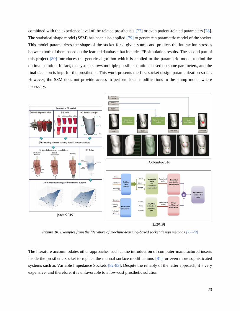
23
combined with the experience level of the related prosthetists [77] or even patient-related parameters [78].
The statistical shape model (SSM) has been also applied [79] to generate a parametric model of the socket.
This model parametrizes the shape of the socket for a given stump and predicts the interaction stresses
between both of them based on the learned database that includes FE simulation results. The second part of
this project [80] introduces the generic algorithm which is applied to the parametric model to find the
optimal solution. In fact, the system shows multiple possible solutions based on some parameters, and the
final decision is kept for the prosthetist. This work presents the first socket design parametrization so far.
However, the SSM does not provide access to perform local modifications to the stump model where
necessary.
Figure 10. Examples from the literature of machine-learning-based socket design methods [77-79]
The literature accommodates other approaches such as the introduction of computer-manufactured inserts
inside the prosthetic socket to replace the manual surface modifications [81], or even more sophisticated
systems such as Variable Impedance Sockets [82-83]. Despite the reliably of the latter approach, it’s very
expensive, and therefore, it is unfavorable to a low-cost prosthetic solution.

24
2.4 Review on the components of the prosthetic CAD/CAM
2.4.1 3D scanning of the residual limb
Measuring the shape of the residual limb by a geometrical 3D-scan could be an important step in a digital
prosthetic design method, since the socket design is very dependent on the unique parameters of the residual
limb, including its geometrical shape.
Figure 11. Examples from the literature of the used 3D-scanning techniques [76, 97, 103, 110]
One of the early attempts to determine the volume of the residual limb has been carried out by Fernie et al.
[84] in 1978 using a water tank. Other authors used the same approach or a tape measure to determine the
stump’s volume [85-86]. With the introduction of the CAD/CAM systems, a new method for limb volume
measurement came to light, using digitizers to create a virtual 3D model of the stump [87-88], and non-
contacting laser scanners have been introduced in this field [89-93]. Recent advances in optical scanning
have led to short-cuts for topology and shape optimization [94], which is necessary because of the difficulty
of securely mounting the residual limb during the scan [95]. Recently, portable laser scanners have been
used and investigated by many authors in the prosthetic application [70, 96-97]. Potable low-cost RGB-

25
Depth sensors such as Microsoft Kinect cameras were also used to create the 3D model of the residual limb
[73-74]. Another proposed approach used a fixed camera to capture the images of the limb of the patient
placed in a turntable, with image processing to produce the stump 3D model from the captured frames [98].
While a 3D geometrical scan provides geometrical data of the external 3D surface of the residual limb,
many other authors considered the need for a volumetric scan to capture its internal anatomical details. This
has been achieved using Medical Resonance Imaging (MRI) or computerized tomography (CT) techniques
[59, 99-103]. Medical imaging is also combined with an optical geometrical scan for a more accurate 3D
shape with anatomical details [69].
Medical imaging solutions allow capturing a detailed level of information related to musculoskeletal
geometries. However, its main drawback is the high cost, making them unfavorable to be integrated into a
complete low-cost prosthetic design and fabrication process. Another disadvantage is the risk of human
body exposure to the ionizing radiation with CT modality [104]. An alternative low-cost and safe solution
for a detailed volumetric scan is the ultrasound imaging techniques [105-107]. This approach often consists
of a rotating ultrasound emitter and receiver that also moves according to the vertical axis. However, the
scanning procedure using this technique is relatively long and takes several minutes to be completed, which
may involve involuntary limb movement or muscles’ contraction during the scan process. Camera-based
motion compensation has been proposed as a solution to this issue [107-110].
2.4.2 Measurement of biomechanical parameters
Biomechanical data, such as soft tissues elasticity parameters, and other physical characteristics, gained the
interest of many researchers and are included in the stump digital model. In the current artisanal practice,
soft tissue stiffness is evaluated by the prosthetist by manual palpation [111]. For a prosthetic CAD process,
numerical values are needed. Some researchers used estimated values extracted from the literature
[73,100,103], whereas others attempt to measure them directly from the patient’s stump. The widely used
technique to quantify the soft tissue characteristics is the mechanical indentation which consists of indenting
the examined material until a certain pressure is formed, and then finding the relationship between the
displacement and the formed pressure. Fischer [112] was the first to propose a device to quantify the
palpation objectively using a force gauge. Biomechanical indentation has seen increasing research focus
throughout the last two decades [113-114]. The biomechanical indentation of human tissue in vivo can be
split into two categories: passive and active.
Passive indenters are generally hand-held devices used to collect hyper-elasticity and/or viscoelasticity
related data through medical imaging techniques [115], elastography [116], or even by using pressure
sensors mounted on the indenter device [117-120]. Active biological indenters are robotic or actuated
devices that are either mounted to an actuated arm [121] or a static base [119,122-125] (Figure 12a). One

26
of the recent researches in this field was the one carried out by MIT developing an elasticity measuring
device called “FitSocket" [59] (Figure 12b).
Figure 12. Examples of limb measurement devices: (a) Active biological indenter mounted in a static base [125];
(b) FitSocket device [59]
The main limitation of passive indenters is the inability to control force and position referenced to the
residual limb which may limit the reliability of the collected data. In contrast, active indenters can control
their position accurately.
2.4.3 Stump/socket interaction measurement
Quantifying the actual stresses on the stump-socket interface during the prosthetic use helps to make an
objective post-fabrication evaluation of the socket. Inappropriate pressure distribution can generate many
discomforts, and high local pressures applied for a long time to the skin may cause skin problems. As the
relationship between stresses and discomfort depending on the subject’s weight, endurance, residual muscle
tonicity, and lifestyle [77], identifying pressure threshold values can be the first step to reduce a potential
discomfort [12]. Many researchers attempted to measure these thresholds [123-130], however, standard
threshold values are not available yet, especially because they depend dramatically upon the unique features
of the patient residuum and its status.
Since the late 1960s, a variety of force transducers have been developed to map the pressure distribution
during/after socket design to assess and improve the socket fit and comfort [131]. One of the main
challenges is selecting suitable transducers for the specific experimental and clinical environment and
choosing the suitable mounting technique [132-133].
Four main types of sensing elements are reported in the literature and used for the quantification of the
stump-socket interaction stresses: strain gauge, piezoresistive, capacitive, and optical-based sensors.

27
Figure 13. Examples of pressure sensors: (a) traditional strain gauge [134]; (b) three common types of FSRs:
Interlink, LuSense, and FlexiForce [141]
Strain Gauges (SGs) are devices used to measure strain on an object. They consist of small patches of
silicone or metal (Figure 13a) with variable electrical resistance in function to any applied mechanical
strains [135]. This type of transducers has been widely used in many applications [136], and was introduced
in lower limb prosthetic applications in the 60s [136], and then widely used by other researchers in the
following years [95,137-138]. SGs are simple, highly sensitive, and light-weighted, and can be used as a
piston-type transducer to measure both normal and shear stresses. However, they are very sensitive and
susceptible to humidity and heat changes [139], and they require a relatively big amount of power to operate
[133,140]. Besides, their stiff backings cause stress concentrations at the sensor edges especially at the
anatomically curved areas [136].
Researchers usually prefer to use piezoresistive transducers because they are thin, flexible, and easy to use.
One of the popular piezoresistive sensors in this field is the Force Sensing Resistor (FSR) [141]. FSRs can
be made in various shapes and sizes (Figure 13b), and thanks to their small size and thinhood, they can be
mounted on the surface of the socket. They are very simple and easy to use and don’t require any
sophisticated electronics to operate. However, this type of sensors can only measure the normal contact
force and may exhibit drift during the use inside the socket, as well as hysteresis effect and high sensitivity
to temperature.
A low temperature-sensitive alternative solution is the capacitive sensor, which consists of a dielectric
material placed between two parallel conductive surfaces. This sensor provides a measurement by either
changing the overlapping surface area between the two conductive surfaces or by changing the distance
between the two conductive surfaces [135]. These sensors have been introduced in the prosthetic
applications and can be installed either inside or outside the socket wall [142-145]. Since these sensors can
be placed embedded inside the socket, no noticeable drift is exhibited during the dynamic measurement of
the stump-socket interaction. They also need very low energy for operation. But on the other hand, like the
piezoresistive sensors, this kind of transducers provide only the measurement of direct uniaxial pressure.

28
Later, triaxial capacitive sensors have been reported but they were expensive, and on the other hand, they
were rigid, which does not comply with the limb geometry [137,146]. Another drawback of these
transducers is their susceptibility to crosstalk noise, especially when arranged in a mesh configuration and
therefore require relatively sophisticated electronics to filter out this noise [147].
Another type of existing pressure sensor used in the medical field is the Fiber Optical Sensors (FOS) [148].
They are used in many applications to measure the strain [149-150], pressure [151], force [152],
temperature [153], and even refractive index [154]. This type of sensor has been used in prosthetic
applications in the last decades [155-157]. The capability of these sensors to measure the stump-socket
interface pressures in-situ was first investigated by Donati et al. in 2013 [158]. Later in 2015, the same
researchers improved the sensor design so it can be inserted within prosthetic sockets to provide an overall
impression of the overall pressure distribution [159]. Optical sensors have shown the ability to measure
both normal and shear stresses [160] and they attracted many researchers for their durability, high
sensitivity, and immunity to electromagnetic interference [161-162]. These sensors, however, are
susceptible to electromagnetic interferences, and their full operation might be hampered in case of any
damage to the optical fiber or optoelectronic components [161].
As for the mounting techniques, literature shows that transducers can be mounted using different
techniques: transducers mounted on socket wall, transducers inserted in the socket, and transducers
embedded in the socket wall (Figure 14).
Figure 14. Transducer mounting techniques: (a) transducer mounted on socket wall through a drilled hole and the
piston extended to be in direct contact with residual limb skin; (b) the same mounting technique with a slight difference
that the piston is flush with the inner socket face and does not penetrate the liner; (c) transducer inserted inside
prosthetic socket; and (d) transducer embedded in the socket wall [163].
The transducers mounted on the socket wall (Figure 14a,b) were used for the first time by Appoldt et al.
[136] and widely investigated and used in the last five decades [95,164-166]. to measure the pressures in
transfemoral sockets. Usually, a strain gauge (SG) is the kind of sensors used in this mounting technique,
which can measure both normal and shear stresses. The main drawback of this technique is the need to

29
modify the socket by making holes to place the sensing elements, as well as the bulkiness of the strain
gauges that adds weight to the socket and alter the gait cycle and affect the accuracy of the interaction
quantification. On the other hand, this technique provides stress measurements in the local areas where the
sensors are placed and dismisses the pressures in the areas in between. To overcome the drawbacks of the
SG-based technique, thin pressure sensors (piezoresistive, capacitive, or optical-based sensors) can be
inserted inside the socket, between the socket and the liner, or sometimes between the liner and the stump
(Figure 14c). This technique does not require socket laborious modifications and can provide continuous
measurement for the whole surface using a sensors’ array, such as the F-Socket system [167]. However,
the sensor placed inside the socket may exhibit drifts during the dynamic tests, therefore, some researchers
studied an alternative mounting technique where the sensor is embedded inside the socket wall (Figure
14d). It is a technique developed by researchers from the Centre for Applied Biomechanics (CAB) at the
University of Malaya, Malaysia, by introducing Fiber Bragg Grating (FBG) sensors in the socket wall
during socket fabrication. These FBG sensors are highly sensitive to dynamic loads and thus they can
translate the received internal strain of the socket wall into internal pressure by inverse problem analysis
approach [168].
2.4.4 Stump/Socket interaction simulation
It is assumed that the simulation of the interaction between the socket and the stump is able to enhance the
ability to numerically design prosthetic sockets [16]. This consists of simulating the static (i.e. standing
posture) or dynamic (i.e. gait cycle) interaction between the stump/socket system to predict the load
distribution in terms of pressure and shear stress at the stump-socket interface during the prosthetic use and
to evaluate the wearability of the socket by verifying the presence of dangerous undercuts that may cause
large tissue deformation during the donning phase [16]. These results will provide an objective way to
assess the socket design and guide the optimization of the socket shape.
Usually, Finite Element (FE) -driven simulations are used in this field as reviewed in [170-171]. FE
method has been identified as a potential method for prediction and evaluation of the load transfer between
the stump and a socket. It allows to examine the stresses in the entire residual limb including the surface
and internal tissues and predict the load transfer prior to socket fabrication. Many researchers in the last
decades have studied the FE method to simulate both the transfemoral [172-175] and transtibial cases [176-
178]. Generally, the finite element analysis includes two separate steps. The first one simulates the residual
limb donning into the socket to obtain the preliminary contact pressures between the two objects, and the
second one, after the first step, starts by applying some load to the socket. In some researches, this applied
force is equal to half of the patient weight mimicking the standing configuration [74, 80, 104, 179-180],
whereas in other works, it is a dynamic force mimicking the applied load during the gait cycle [73,181,
182].

30
Figure 15. Examples from the literature of FE simulations of the stump-socket interaction [178.179,181,182]
The modeling of the stump/socket system is not a simple task since there are many critical conditions to be
considered, such as the non-linear elastic property of the biological stump soft tissues as well as the hard
contact conditions due to the irregular geometry of the stump surface. It has been reported that both the
mechanical properties of the residual limb and the socket model are important for reliable simulation results
[183]. The human limb is not a simple object showing very complex anatomy consisting of a variety of
inhomogeneous material such as the dermal layer, the soft tissues including fat and muscles, bones, tendons,
nerves, and blood vessels… etc., and each part has complex physical and biomechanical properties. Some
researchers modeled the entire volume of the stump soft tissues (excluding the bones) as a homogeneous
non-linear hyperplastic deformable material [172, 184], others used the non-linear viscoelastic model [185],
whereas some developed a detailed model based on MRI data [104, 186]. Most of the FE studies simplify
the stump soft tissues as a homogenous linear elastic material [73, 171, 180, 187-190]. Colombo et al. [191]
verified the use of the simplified linear model by the fact that it gave them similar results compared to the
hyperplastic model with the potential energy of deformation expressed by a second-order polynomial, but
its calculation time was 400% faster.
2.4.5 Socket modeling
Many researchers work on developing CAD tools to design the 3D model of the prosthetic socket. In
general, the modeling approach is based on the design rules of the conventional method, where the socket
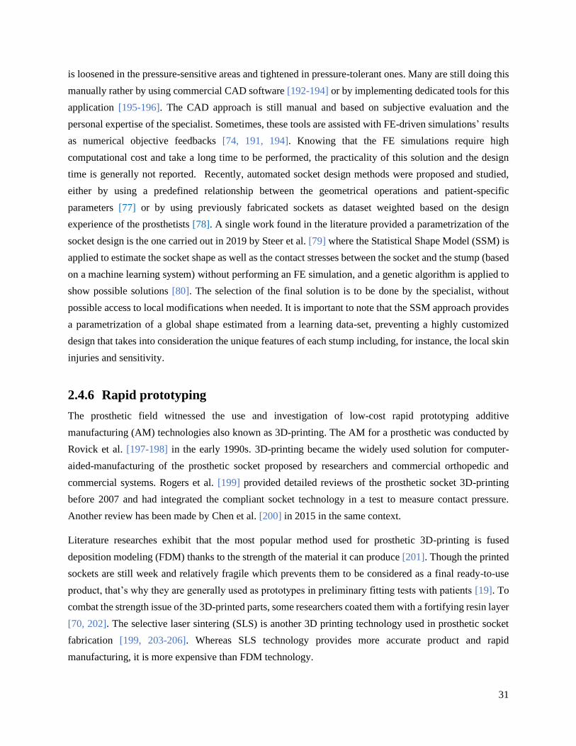
31
is loosened in the pressure-sensitive areas and tightened in pressure-tolerant ones. Many are still doing this
manually rather by using commercial CAD software [192-194] or by implementing dedicated tools for this
application [195-196]. The CAD approach is still manual and based on subjective evaluation and the
personal expertise of the specialist. Sometimes, these tools are assisted with FE-driven simulations’ results
as numerical objective feedbacks [74, 191, 194]. Knowing that the FE simulations require high
computational cost and take a long time to be performed, the practicality of this solution and the design
time is generally not reported. Recently, automated socket design methods were proposed and studied,
either by using a predefined relationship between the geometrical operations and patient-specific
parameters [77] or by using previously fabricated sockets as dataset weighted based on the design
experience of the prosthetists [78]. A single work found in the literature provided a parametrization of the
socket design is the one carried out in 2019 by Steer et al. [79] where the Statistical Shape Model (SSM) is
applied to estimate the socket shape as well as the contact stresses between the socket and the stump (based
on a machine learning system) without performing an FE simulation, and a genetic algorithm is applied to
show possible solutions [80]. The selection of the final solution is to be done by the specialist, without
possible access to local modifications when needed. It is important to note that the SSM approach provides
a parametrization of a global shape estimated from a learning data-set, preventing a highly customized
design that takes into consideration the unique features of each stump including, for instance, the local skin
injuries and sensitivity.
2.4.6 Rapid prototyping
The prosthetic field witnessed the use and investigation of low-cost rapid prototyping additive
manufacturing (AM) technologies also known as 3D-printing. The AM for a prosthetic was conducted by
Rovick et al. [197-198] in the early 1990s. 3D-printing became the widely used solution for computer-
aided-manufacturing of the prosthetic socket proposed by researchers and commercial orthopedic and
commercial systems. Rogers et al. [199] provided detailed reviews of the prosthetic socket 3D-printing
before 2007 and had integrated the compliant socket technology in a test to measure contact pressure.
Another review has been made by Chen et al. [200] in 2015 in the same context.
Literature researches exhibit that the most popular method used for prosthetic 3D-printing is fused
deposition modeling (FDM) thanks to the strength of the material it can produce [201]. Though the printed
sockets are still week and relatively fragile which prevents them to be considered as a final ready-to-use
product, that’s why they are generally used as prototypes in preliminary fitting tests with patients [19]. To
combat the strength issue of the 3D-printed parts, some researchers coated them with a fortifying resin layer
[70, 202]. The selective laser sintering (SLS) is another 3D printing technology used in prosthetic socket
fabrication [199, 203-206]. Whereas SLS technology provides more accurate product and rapid
manufacturing, it is more expensive than FDM technology.

32
The 3D-printing is the widely used computer-aided manufacturing (CAM) technique to realize a
numerically designed prosthetic socket. One of its benefits is that it allows adding any interesting
affordances to the socket such as cooling channels [63]. Another benefit is its wide range of material
selection showing a variety of material characteristics and properties [207].
2.5 Discussion
The field of prosthetics dramatically evolved in the last decades, but still, many amputees reject their
prosthetic devices due to socket-related issues, as discussed previously. Since the problem resides on the
currently applied socket design approach that is mainly grounded on the prosthetist’s experience, with poor
attention to quantitative, many researchers are working toward an alternative numerical-based approach,
involving computer-aided design (CAD) and computer-aided manufacturing (CAM) techniques.
CAD/CAM of prosthetics has been available since the 1980s though acceptance has been slow [199]. Still,
very few researchers studied a complete numerical socket design process. And generally, such projects did
not yet rise to a clinically practical level. Most of the proposed solutions, as well as the existing commercial
CAD/CAM solutions, such as Create O&P (https://www.createoandp.com/), Canfit™ O&P
(https://vorum.com/canfit-op-cad-software/), and Rodin4D (https://www.rodin4d.com/), provide CAD
tools for the manual design of the socket by manually manipulating the 3D shape of the scanned residual
limb. However, these systems do not offer any kind of assistance to the prosthetists. All the decisions and
actions are taken based on their experience and personal skills, and so multiple trial/rectifications sessions
are still required. Thus, the two main problematics of the current socket design practice, which are the time-
consuming iterative modification process and the high dependence on the know-how of high-cost expertise,
are not yet resolved. Several researchers studied the possibility of measuring the stump-socket interaction
by different types of pressure sensors [162], to objectively assess a fabricated socket, but this approach
consists of a post-fabrication step which does offer solutions for the design-related problematic. The
outcomes of FE simulations were introduced as numerical feedback of the socket design for the sake of
objectivity [75, 190, 193], and also introduced in a complete virtual platform for prosthetic design [72-74].
However, the simulations’ speed, the processing time, and the practicality of this approach were not
reported, knowing that the FE simulations are usually expensive and sometimes take forever to be
performed. Recently, the machine learning approach has been introduced [78, 79, 124, 196] to estimate
either the shape of the socket or even the stump-socket interaction stresses without the need for simulations.
This provides a fully numerical approach for the socket design that eliminates the manual shaping step and
the iterative trial/rectifications steps and also provides a lower dependence on the expertise. However, this
approach generally relies on a learning database consisting of sockets fabricated using the conventional
method that were not subject to an objective evaluation. Moreover, the parametrization of the socket shape
using SSM [78-79] does not provide a detailed model for the socket design that includes every possible
33
local modification, because the SSM provides global parametrization based on the most influential Principal
Components (PC), ignoring all the other PCs that have a small influence to the overall model shape.
The current thesis is an attempt to fill the gaps exhibited in the state-of-the-art. We are going to propose
and investigate a complete digital socket design workflow that consists of the three mains steps: scan of the
residuum, stump modeling, and socket design (Figure 2).
The proposed approach will maintain the same conventional rules related to the socket surface shaping
starting from the scanned replica of the stump. However, whereas no numerical standards are yet established
to rule the designing process, and the final socket evaluation is often dependent upon the patient’s subjective
feedback, we are going to postulate analytical constraints as a numerical definition of the well-fit socket
shape. Consequently, the socket design problem is transformed into a Constraint Satisfaction Problem
(CSP). These constraints will be the base of a numerical design assistant, for a real-time calculation of them
during the shaping process will provide real-time numerical feedback to objectively assess the designer. A
fast calculation is possible thanks to the use of a simple Mass-Spring -based system instead of the Finite
Element approach to model the residual limb, along with an inverse stump-socket interaction calculation to
eliminate the expensive contact formulation that slows down the calculation.
The overall process will be completely based on the virtual replica of the patient’s stump including its
geometry, physical properties, and even the distribution of the pressure-sensitivity on its surface. The
dependence on the skills of a specialist is thus reduced significantly, and the socket design provided by the
system, proposed in this project, is highly customized to the patient’s stump. The design time is reduced
from several days [46] to nearly half-hour.

34
Modeling of the Stump Soft-Tissues and
Stump-Socket Interaction
A prosthetic CAD process is mainly based on the virtual model of the patient’s residuum. This model is
usually used to calculate the socket-stump interaction and predict the interaction stresses in the residual
limb surface as a numerical indicator of the socket fit-quality. Generally, the Finite Element Method (FEM)
is used for this purpose. One of the main drawbacks of this method is its high computational cost, making
it very difficult to perform fast calculations during an interactive or even automated design process. In this
chapter, we introduce previously employed physically-based models in the topic of soft tissue modeling for
biomedical simulations, and then we propose a new modeling method based on the Masse-Spring System
(MSS) for fast soft-tissues deformation. A discrete collision detection (DCD) algorithm is also introduced
for the stump-socket contact modeling. A comparison between the outcomes of this model and those of the
FE are compared for validation.
3.1 Simulation of deformable objects in biomechanics
In the mechanics of materials, deformable objects are objects that exhibit a change of size or shape when
are subject to a mechanical load. Deformable objects can be defined generally in terms of linear and non-
linear stress-strain relationships, meaning that their behavior is linear if the body undergoes a small
deformation and strongly non-linear if the body is deformed above the linear limit.
Soft tissues are deformable objects that have several properties such as non-compressibility and
viscoelasticity. Their stress-strain relationship depends strongly on the type of tissue and conditions of the
physical experiments [208]. Usually, the soft tissues are modeled as three-dimensional material for which
non-linear continuum mechanics is used as the fundamental basis [209-210]. Soft tissues behave
anisotropically because their fibers usually tend to have preferred directions. They usually show viscoelastic
behavior, which has been associated with the shear interaction of collagen with the matrix of proteoglycans
[211]. At a microscopic level, they are non-homogeneous materials because of their composition.
The knowledge about the mechanical properties of the human body and the simulation of soft tissues
mechanical behavior are crucial for many fields. The literature review shows several methods used by the
researchers to model the biomechanical behavior of soft tissues: the finite element method, position-based
dynamics, meshless deformations, and mass-spring system.

35
3.1.1 Finite element method
The finite element method (FEM), also known as finite element analysis (FEA), is described in detail in a
book of K.J. Bathe [212]. It is the most widely used method for solving problems of engineering and
mathematical models, including those in the medical environment. It computes approximations of real
solutions to partial differential equations (PDE), called basis functions. To solve a problem, the FEM
subdivides a large system into smaller, simpler parts that are called finite elements. The usage of FEM in
medical fields was perfected by the authors over the years. In 1996, FEM is used by Cotin et al. [213] in
the development of a virtual surgical environment. It has been used also in the simulation of breast soft-
tissue deformations [214-217], of foot soft tissues during standing, walking, for insole design, or even for
female high heel shoe design [218-222], as well as in the prosthetic socket design application as previously
described.
3.1.2 Position-based dynamics
Position based dynamics (PBD) was first introduced by Jakobsen [223] in 2001, where a cloth system was
introduced based on constraints to keep particles at a certain distance. The method was described by Müller
[224] in 2005 and then it was given its current name in 2007 [225].
For a discretized object consisting of a set of particles, the PBD, as the name already indicates, works
directly with the positions of those particles instead of their forces. At each simulation step, the new particle
positions are estimated using explicit integration, then some predefined constraints are projected over the
estimated positions to calculate the final positions to which the particles are moved. This approach has been
widely used in the simulation of cloth deformations, hair, fluids, and other deformable shapes [226]. The
advantage of the PBD is its unconditional stability offering the possibility to use large simulation time-
steps. It is a stable and controllable method, perfect to use in virtual environments, where user interactions
are applied. However, it is not physically accurate, since it does not depend solely upon physical properties
and formulations, but also on other factors like the predefined constraints, the time-step size, and the number
of iterations performed by the solver. For these reasons, the PBD is often used in an approximate simulation
of deformable bodies. The PBD outcomes are visually satisfying, that’s why it is favorable in graphics and
video game applications.
3.1.3 Meshless deformations
This approach is based on the shape matching technique, where the energies and forces from the classical
approach are replaced by geometric constraints and distances from current to goal positions respectively. It
was introduced and described by Müller et al. [224]. Instead of a classical mesh, each object is represented
by a point-cloud. The extended shape matching technique allows us to model the elasticity of material by
pulling the points towards the goal configuration.

36
The method is suitable to simulate multiple deformable bodies, but more for gaming purposes due to the
lack of accuracy of the simulation. Such a method is useful especially in the simulation of fluids, but also
to model the plasticity of the material.
3.1.4 Mass-springs-system
Mass Spring System (MSS) is a fairly simple model, incorporating our knowledge about physical laws
based on the continuum mechanics into an uncomplicated system of point-masses interconnected by
springs. In MSS, a deformable body is represented by a set of punctual masses, called nodes, each defined
by its “mass” and its position vector, interconnected together by springs each defined by its “initial length”
and “stiffness”. A damping property could be added to absorb the energy of the system during a time-
dependent dynamic simulation. This system is sometimes noted Mass-Spring-Damper (MSD) system [227].
It corresponds to the Kelvin-Voigt model for linear viscoelastic materials and it is illustrated in Figure 16.
Figure 16. The elastic connection between 2 punctual masses in MSS, with initial length L0, stiffness k, and damping
coefficient c
Despite its limitations derived from its simplicity, MSS has been widely used to simulate the behavior of
deformable objects in many applications, such as in computer graphics to simulate cloth and other
deformable solids [228-231], as well as for facial expressions [232]. MSS is very simple and easy to
implement and consumes lower computational resources than the FE approach while exhibiting higher
physical accuracy than both the PBD and meshless approach. That’s why it has been eagerly used in medical
applications to model the human soft tissues and in developing virtual surgical environments [227,233-237]
as a real-time performing model. No previous work reported in the literature used this model in the lower
limb prosthetic field.
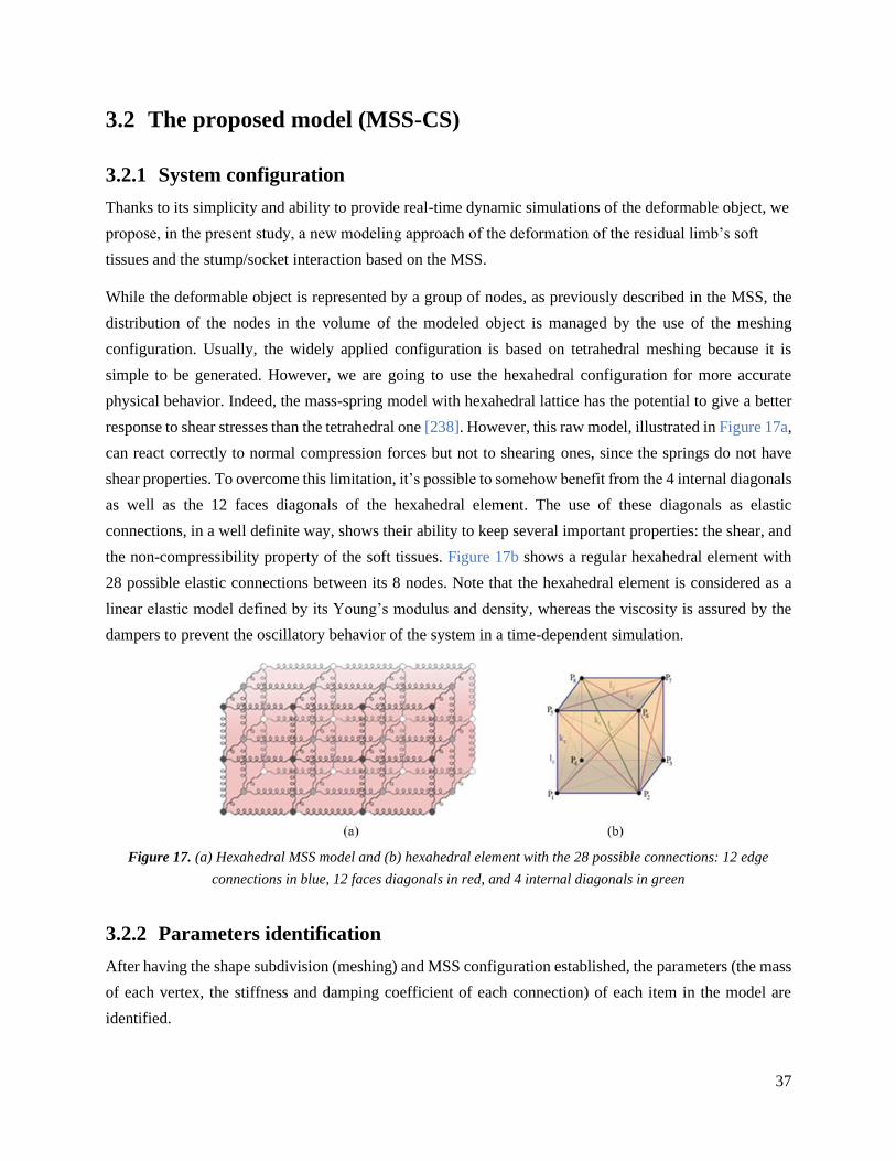
37
3.2 The proposed model (MSS-CS)
3.2.1 System configuration
Thanks to its simplicity and ability to provide real-time dynamic simulations of the deformable object, we
propose, in the present study, a new modeling approach of the deformation of the residual limb’s soft
tissues and the stump/socket interaction based on the MSS.
While the deformable object is represented by a group of nodes, as previously described in the MSS, the
distribution of the nodes in the volume of the modeled object is managed by the use of the meshing
configuration. Usually, the widely applied configuration is based on tetrahedral meshing because it is
simple to be generated. However, we are going to use the hexahedral configuration for more accurate
physical behavior. Indeed, the mass-spring model with hexahedral lattice has the potential to give a better
response to shear stresses than the tetrahedral one [238]. However, this raw model, illustrated in Figure 17a,
can react correctly to normal compression forces but not to shearing ones, since the springs do not have
shear properties. To overcome this limitation, it’s possible to somehow benefit from the 4 internal diagonals
as well as the 12 faces diagonals of the hexahedral element. The use of these diagonals as elastic
connections, in a well definite way, shows their ability to keep several important properties: the shear, and
the non-compressibility property of the soft tissues. Figure 17b shows a regular hexahedral element with
28 possible elastic connections between its 8 nodes. Note that the hexahedral element is considered as a
linear elastic model defined by its Young’s modulus and density, whereas the viscosity is assured by the
dampers to prevent the oscillatory behavior of the system in a time-dependent simulation.
Figure 17. (a) Hexahedral MSS model and (b) hexahedral element with the 28 possible connections: 12 edge
connections in blue, 12 faces diagonals in red, and 4 internal diagonals in green
3.2.2 Parameters identification
After having the shape subdivision (meshing) and MSS configuration established, the parameters (the mass
of each vertex, the stiffness and damping coefficient of each connection) of each item in the model are
identified.

38
Mass:
To find the mass mi of vertex i, we used the following formula presented by Deussen et al. [239] as follows:
𝑚𝑖 =1
8∑ 𝜌𝑗𝑉𝑗𝐻 (1)
where H is the group of hexahedral elements to which the vertex i belongs, j and Vj are the density and
volume of the hexahedral element j that belongs to H respectively. This equation means that the mass of
each hexahedral element is equally distributed to its 8 nodes. If a node is shared by multiple elements, its
mass will be equal to the sum of the one-eighths of the mass of each of these elements.
Stiffness:
To calculate the stiffness of each spring in the system, we referred to the formulation presented by Golec
[240] in 2018. Referring to the hexahedral element shown in Figure 17b, there are three types of connections
(edges, internal diagonals, face diagonals) with stiffness constants ke, kc, and kf respectively. The values of
these parameters were identified using the following formulations:
{
𝑘𝑐 =
3𝐸𝑙𝑒10 + 7.5𝐴
=√3𝐸𝑙𝑐
10 + 7.5𝐴
𝑘𝑓 =1.5𝐴𝐸𝑙𝑒10 + 7.5𝐴
=1.5𝐴𝐸𝑙𝑓
√2(10 + 7.5𝐴)
𝑘𝑒 =0.75𝐴𝐸𝑙𝑒10 + 7.5𝐴
+2𝐸𝑙𝑒
10 + 7.5𝐴
(2)
where E is the young modulus assigned to the hexahedral element, and le is the length of its edge considering
that this is a regular cubical element. A is a parameter to be manually tuned. Golec [240] proved that the
model shows the same results for any given value to A between 0.1 and 100. If a connection is shared by
multiple hexahedral elements, its stiffness is equal to the sum of the corresponding quantities calculated for
each hexahedral element according to equation 2.
Damping coefficient:
To ensure the best behavior consistency for different and combined resolutions [240-243], the damping
coefficient ci, of a spring of index i and stiffness ki connecting two punctual masses mi1 and mi2 with initial
length li0, is expressed in the following equation:
𝑐𝑖 =2√𝑘𝑖(𝑚𝑖1+𝑚𝑖2)
𝑙𝑖0 (3)

39
3.2.3 Volume conservation
Soft tissues are incompressible materials, i.e. their volume remains constant under external and internal
loadings. For this kind of material, the Poisson’s Modulus tends to 0.5, while the system defined in equation
2 deals only with a Poisson’s modulus equal to 0.25 [238, 240]. To solve this problem, a novel approach,
called MSS-CS (Mass-Spring System Corrective Springs), was developed in this study. In fact, additional
springs, named “Corrective Springs” were integrated to the MSS model. Thus, the proposed configuration
consists of adding, in parallel with the internal diagonal springs with stiffness kc and initial length lc (resp.
the face diagonal springs with stiffness kf and initial length lf), new springs having stiffness k’c and initial
length l’c (resp. stiffness k’f and initial length l’f). Constitutive equations of our MSS-CS are based on two
conditions, which are described below:
Condition 1: The initial lengths of these additional springs are greater than the initial geometric lengths
as follows:
𝑙′𝑐𝑙𝑐=𝑙′𝑓
𝑙𝑓= 𝛼 𝑤𝑖𝑡ℎ 𝛼 > 1 (4)
This condition allows added springs to be always extended to conserve the volume (Figure
18).
Condition 2: The stiffness of each of these springs is calculated in terms of the volume variation as
follows:
𝛿𝑣 = 𝑉𝑐 − 𝑉0𝑉0
(5)
with V0 and Vc are the initial and actual volume of the hexahedral element respectively.
The corrective spring’s stiffness is defined as follows:
𝑘′𝑓 = 𝑘′𝑐 = 𝐶 𝐸𝑙𝑒(𝛿𝑣)
(6)
with C and are constants to be identified.
Supposing that the hexahedral element is regular, i.e. a cube, then:
𝑙𝑒 = √𝑉3
0 (7)
Therefore:

40
𝑘′𝑓 = 𝑘′𝑐 = 𝐶 𝐸 √𝑉0
3 (𝑉𝑐−𝑉0
𝑉0)
(8)
Finally, our proposed model is then defined by the equations 2, 4, and 8, with four constants A, , C and
to be determined. By applying manual tuning on a simple cubical element, the obtained values of these
constants are: A=0.5, = 1.4, C = 25, =2.
Figure 18. Cubical elastic object subject to normal compression pressure: (a) Compressible material modeled using
MSS without corrective springs. (b) Uncompressible material modeled using MSS with corrective springs performing
horizontal expansion to conserve its volume
3.2.4 Simulation algorithm
Let N be the total number of vertices in the MSS-CS model. Two types of forces are applied upon each
vertex of index i: internal forces noted Fiint, applied by the related elastic connections and known to be
equal to (𝐾𝑖𝑈𝑖 + 𝐶𝑖��𝑖), and external forces, noted Fiext (where Ki is the stiffness matric, Ci is the damping
matrix, Ui is the displacement vector and ��𝒊 is its derivative). Let Mi be the mass matrix of the vertex i,
and Ai its acceleration vector which is known to be equal to the second derivative ��𝒊 of the displacement
vector. Therefore, according to the second law of Newton, the equilibrium equation is defined as follows:
𝐾𝑖𝑈𝑖 + 𝐶𝑖��𝑖 + 𝐹𝑒𝑥𝑡𝑖 = 𝑀𝑖��𝑖 (9)
Integration is to be applied to solve the differential equation 9 and then find the new position of the vertex
i in each simulation step t. We chose the implicit Euler integration method that gives a more stable
simulation than the explicit one. A first-order linearization is performed since the forces are non-linear
according to the position variable. Applying these steps on all N vertices of the system, we get a system of
3N linear equations with 3N unknowns. The matrix of such a system is always symmetric positive definite.
Therefore, we can solve the system using the Conjugate Gradient method.

41
3.3 Interaction with rigid body
3.3.1 Socket modeling
To simplify the implementation and reduce the computational cost, the socket is considered as a rigid body.
Usually, sockets are made of perlon stockinette hardened by resin, which makes it firmly stiff and non-
deformable.
Figure 19. The 3D triangular surface of a transtibial prosthetic socket: (a) shaded view; (b) wireframe view
Beside its triangular 3D surface (Figure 19), the rigid socket is characterized by the following physical
parameters: mass Ms, moment of inertia Is, center of mass CM, and center of inertia Cs. The behavior of the
socket in the 3D space is described by the following second law of Newton:
𝐹𝑠 = 𝑀𝑠𝑎𝑠 𝑎𝑛𝑑 𝜏𝑠 = 𝐼𝑠𝛼𝑠 (10)
where Fs is the sum of all forces applied to the socket, s is the sum of all torques applied to the socket, as
and s are the linear and angular accelerations of the socket respectively.
3.3.2 Contact modeling
Modeling contact between two 3D objects includes two numerical processing components: 1) a collision
detection algorithm and 2) a formulation of physical response.
3.3.2.1 Collision detection algorithm
A node-to-triangle discrete collision detection algorithm was established. In this method, a collision occurs
when the point penetrates the triangle, i.e. it passes through the triangle from the positive side of the
triangle’s plane to the negative one (Figure 20).

42
Figure 20. Schematic representation of the collision taking place between the point Pi and the triangle Tj
Thus, in each simulation time-step, the involved point is checked to verify if this point is behind the
triangle’s plane and whether its projection to this plane is inside the triangle (Figure 20). In other words,
we trace a ray from the point in the 3D space and verify whether it intersects with the triangle and whether
the point is behind this triangle. Noting that, in our method, the ray is to be parallel to the triangle’s normal
vector. Practically, a collision occurs between a point Pi of the stump and a triangle Tj of the socket if these
following equations are true:
{
𝑉0,𝑗𝑃𝑖 . 𝑁𝑗 ≤ 0
0 ≤ 𝑢 ≤ 1 0 ≤ 𝑣 ≤ 1 0 ≤ 𝑢 + 𝑣 ≤ 1
(11)
where V0,j , V1,j , V2,j are the three points of the triangle Tj. u and v are the barycentric coordinates of the
projection Prij of the point Pi to the triangle Tj. These coordinates define the position of the projection point
with respect to the three triangle’s vertices as follows:
𝑃𝑟𝑖𝑗 = 𝑉0𝑗 + 𝑢 (𝑉1𝑗 − 𝑉0𝑗) + 𝑣 (𝑉2𝑗 − 𝑉0𝑗) (12)
Figure 21. collision detected between the point Pi and the triangle Tj

43
In equation 11, the first inequality means that the point is behind the triangle. The remaining three
inequalities confirm that the projection point to the triangle’s plane is inside the triangle. If all these
inequalities are true, the point Pi and the triangle Tj are considered as “contact pair”. In case if these
conditions are satisfied between Pi and multiple triangles, the nearest triangle to the point is selected.
Basically, the test is applied between each point of the stump surface and each triangle of the socket. Having
N points and M triangles, the complexity, in this case, will be O(NxM), which increases exponentially when
the resolution of meshes increases. The final step in the collision detection phase is placing the point of
each contact pair on a well-selected collision-free position. In our method, we choose the projection of this
point to the triangle as the corrected position.
3.3.2.2 2) Formulation of physical response
Physical response or reaction of the collision consists of all the forces applied to the socket and the stump
due to the collision. Basically, this mechanical reaction consists of two types of forces: the normal contact
force, and the friction force. According to the third law of Newton, the forces applied to the elements of the
contact pair are equal in magnitude and opposite in direction. Thus, having selected Nc contact pairs in the
first phase, for each contact pair Ck (k {1, 2, 3, …., Nc}), the point Pk and the triangle Tk are each subject
to a contact force of magnitude 𝑭𝒄𝒐𝒏𝒕𝒌 and friction of magnitude 𝑭𝒇𝒓𝒊𝒄
𝒌 . Thus, the force applied by the
point of the stump surface to the contact surface of the socket is equal to the sum of the inner forces �� 𝒊𝒏𝒕,𝑷𝒌
applied to the point due to the material mechanical properties along with the external forces �� 𝒆𝒙𝒕,𝑷𝒌. This
total force applied to the point is noted �� 𝑷𝒌 and expressed in the following equation:
𝐹 𝑃𝑘 = 𝐹 𝑖𝑛𝑡,𝑃𝑘 + 𝐹
𝑒𝑥𝑡,𝑃𝑘 (13)
Talking about a normal contact force, we will consider the forces perpendicular to the triangle and discard
the forces aligned with it. Therefore, the magnitude of the contact force is defined as follows:
𝐹𝑐𝑜𝑛𝑡𝑘 = −𝐹 𝑃𝑘 . 𝑁𝐾
(14)
The minus sign in equation 14 is added to obtain a positive value, since the force �� 𝑷𝒌 applied to the point
should be pushing the triangle, having the opposite direction of the triangle normal vector 𝑵𝑲 (Figure 22a).
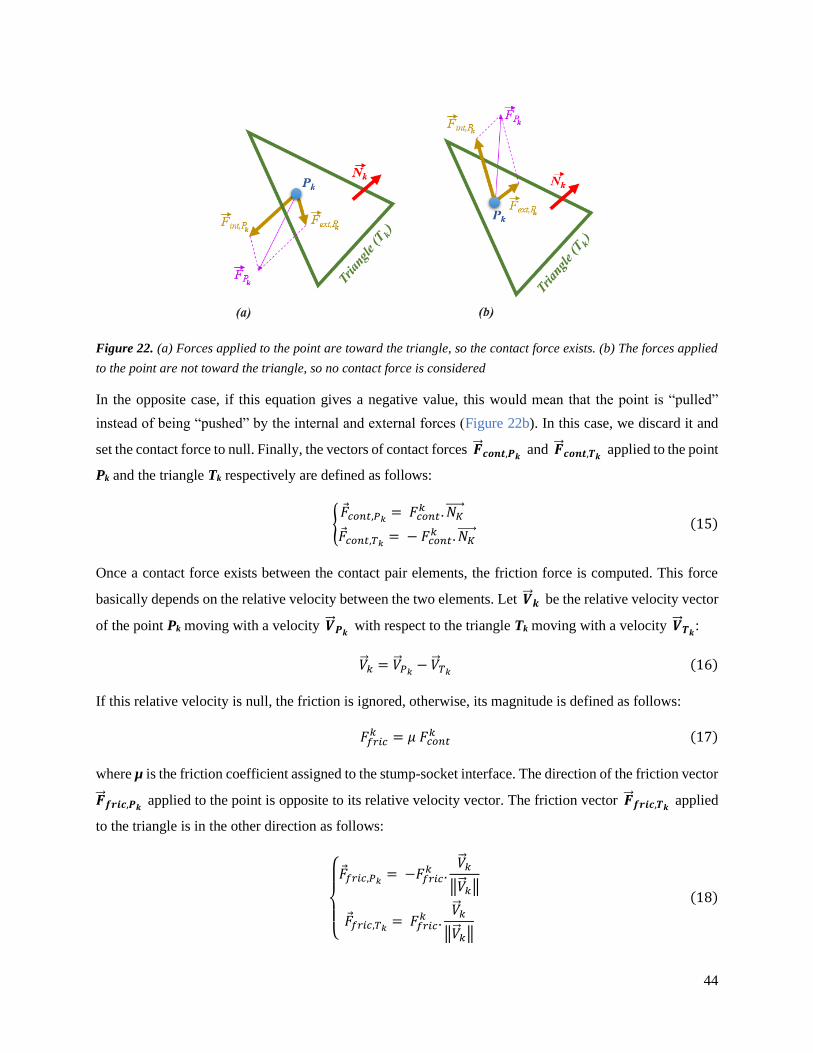
44
Figure 22. (a) Forces applied to the point are toward the triangle, so the contact force exists. (b) The forces applied
to the point are not toward the triangle, so no contact force is considered
In the opposite case, if this equation gives a negative value, this would mean that the point is “pulled”
instead of being “pushed” by the internal and external forces (Figure 22b). In this case, we discard it and
set the contact force to null. Finally, the vectors of contact forces �� 𝒄𝒐𝒏𝒕,𝑷𝒌 and �� 𝒄𝒐𝒏𝒕,𝑻𝒌 applied to the point
Pk and the triangle Tk respectively are defined as follows:
{𝐹 𝑐𝑜𝑛𝑡,𝑃𝑘 = 𝐹𝑐𝑜𝑛𝑡
𝑘 . 𝑁𝐾
𝐹 𝑐𝑜𝑛𝑡,𝑇𝑘 = − 𝐹𝑐𝑜𝑛𝑡𝑘 . 𝑁𝐾
(15)
Once a contact force exists between the contact pair elements, the friction force is computed. This force
basically depends on the relative velocity between the two elements. Let �� 𝒌 be the relative velocity vector
of the point Pk moving with a velocity �� 𝑷𝒌 with respect to the triangle Tk moving with a velocity �� 𝑻𝒌:
�� 𝑘 = �� 𝑃𝑘 − �� 𝑇𝑘 (16)
If this relative velocity is null, the friction is ignored, otherwise, its magnitude is defined as follows:
𝐹𝑓𝑟𝑖𝑐𝑘 = 𝜇 𝐹𝑐𝑜𝑛𝑡
𝑘 (17)
where µ is the friction coefficient assigned to the stump-socket interface. The direction of the friction vector
�� 𝒇𝒓𝒊𝒄,𝑷𝒌 applied to the point is opposite to its relative velocity vector. The friction vector �� 𝒇𝒓𝒊𝒄,𝑻𝒌 applied
to the triangle is in the other direction as follows:
{
𝐹 𝑓𝑟𝑖𝑐,𝑃𝑘 = −𝐹𝑓𝑟𝑖𝑐
𝑘 .�� 𝑘
‖�� 𝑘‖
𝐹 𝑓𝑟𝑖𝑐,𝑇𝑘 = 𝐹𝑓𝑟𝑖𝑐𝑘 .
�� 𝑘
‖�� 𝑘‖
(18)

45
The forces generated by the collision between the elements of each contact pair are thus calculated. To
introduce them to the simulation, we apply the following two steps:
Step 1: For each point Pk of the contact pair Ck and existing on the surface of the stump model, the contact
force �� 𝒄𝒐𝒏𝒕,𝑷𝒌 and the friction �� 𝒇𝒓𝒊𝒄,𝑷𝒌 are added to the external forces in equation 9.
Step 2: Regarding the socket, two vectors are necessary to simulate its behavior in the 3D space: the total
force 𝑭𝒔 and the total torque 𝝉𝒔 , as shown in equation 10. The total force is simply found by summation
of the forces applied to the triangles Tk, k {1, 2, 3, …., Nc}, along with any other external force �� 𝑺,𝒆𝒙𝒕
applied to the socket as follows:
𝐹𝑠 = 𝐹 𝑆,𝑒𝑥𝑡 + ∑(𝐹 𝑐𝑜𝑛𝑡,𝑇𝑘 + 𝐹 𝑓𝑟𝑖𝑐,𝑇𝑘)
𝑁𝐶
𝑘=1
(19)
For the torque, let first consider for each contact pair Ck a torque k that is generated by the interaction of
Pk and Tk and defined as follows:
𝜏𝑘 = (𝐹 𝑐𝑜𝑛𝑡,𝑇𝑘 + 𝐹 𝑓𝑟𝑖𝑐,𝑇𝑘). 𝑃𝑘𝐶𝐼
(20)
where CI is the center of the inertia of the socket. The total torque is then the summation of all these
particular torques with any other external torque s,ext that may exist:
𝜏𝑠 = 𝜏𝑠,𝑒𝑥𝑡 + ∑ 𝜏𝑘
𝑁𝐶
𝑘=1
(21)
3.4 Development of simulation environment
3.4.1 Implementation
A simulation environment was developed using the C++ programming language. Object-oriented
programming was used to define the data structure of the MSS-CS deformable 3D object, which will be the
stump, as well as the 3D rigid object, which will be the socket. For the bony structures of the residual limb
model, the related nodes inside the MSS-CS model are constrained by making them fixed in the Euclidean
3D space. The simulation algorithm for the stump deformation along with its interaction with the rigid
socket is implemented.
The graphical user interface was designed and developed with “Visual Studio / Windows Form
Application”, and OpenGL library [244] was used for the 3D rendering. This interface allows to run and
visualize a simulation with predefined parameters, as well as providing real-time interaction tools for the

46
user to apply instant loads somewhere on the stump surface and also to the socket. The interface of this
simulation environment is shown in Figure 23.
Figure 23. The graphical user interface of the developed simulation environment
3.4.2 The Stump’s Model
A virtual transtibial residual limb was fabricated from a CT dataset [245]. As shown in Figure 24, 3D
geometrical models of both bones and skins have been generated from the CT images using 3D Slicer and
Embido3D.com platforms. The models have been processed to keep one of the two legs and smoothed to
remove the artifacts using the Poisson and Scale-Space surface reconstruction algorithms implemented as
will be described in the next chapter. The hexahedral mesh of the stump volume has been generated using
the IA-FEmesh [246]. Since the stump has generally a cylindrical based-shape, we wrote a C++ code for a
template meshing block whose dimensions are automatically adjusted in function of the stump model
dimensions. Finally, the hexahedral mesh was given to our program to create the related MSS-CS. The
model of the bones has also been introduced in the model generation process, where the nodes of the MSS-
CS model existing within the bones’ volume were constrained in the space, noting that the bones were
already given perfectly aligned with the stump skin model in the first stage.
The parameters of the MSS-CS model were chosen to reflect the physical properties of the soft tissues. For
instance, we used a Young’ modulus of 50KPa, which is a value within the range of soft tissues elasticity

47
modulus values [75, 247], and a density of 1060Kg/m3 which is reported as the density of human soft
tissues in [248].
Figure 24. the reconstruction process of the stump's model from CT images
For the socket, our simulation program is able to import any CAD model saved in STL format. It has been
generated by applying a geometrical process: the stump geometry was used to extrapolate the socket
geometry with few modifications and a thickness of 8 mm. (Figure 19).
3.4.3 Simulation Stability
Evaluation of the simulation’s stability facilitates the choice of the maximum simulation time-step that
provides a compromise between the calculation convergence and the calculation speed. A small simulation
time-step assures a stable but slower simulation than the real-time. On the other hand, the simulation speed
is increased using a large time-step, however, the system may, in this case, gain additional energy at each
step causing increased oscillations and thus the model “explosion”.
There exist several methods to compute the stability of a numerical integration scheme. In the case of the
first-order schemes, we can study a linear test equation ��(𝑡) = . 𝑥(𝑡), where Γ ∈ ℂ is a parameter
mimicking the eigenvalues of linear systems of differential equations. We know that the system is stable if

48
|1 − . ∆𝑡| ≤ 1 [240], where t represents the simulation time-step. The stability of backward (implicit)
and forward (explicit) Euler schemes can be then depicted as shown on the well-known charts in Figure 25,
where the stability regions are the colored ones.
Figure 25. The stability regions for backward (left) and forward (right) [240]
The stability of the semi-implicit Euler method can be evaluated in a slightly more complicated way.
Besides, even though our system uses generally the implicit Euler integration method, it is important to
note that the “Corrective Springs” formulations are explicitly integrated into the system equations since
they are non-linear as a function of position variation and it was not possible to linearise them in the first
order. Therefore, the analytical evaluation of our system’s stability is a complex task. The simulation time-
step has been chosen using a heuristic trial-error method starting from a large time-step for a high simulation
speed, and then gradually decreasing it until achieving a visually stable simulation.
3.5 Accuracy analysis
Two simulation cases were developed to evaluate the accuracy of our soft tissue deformation and stump-
socket interaction algorithms. We started first with a simple cubical elastic object subject to normal
compression due to the weight of a rigid box (Figure 26a). We repeated the simulation with different weight
values, and we recorded, for each one, the displacement and contact pressure on the elastic cube’s upper
surface as well as its volume variation, and we compared them to analytical results. We also implemented
the” Mass-Spring System – Corrective Forces” (MSS-CF) model developed by Golec [240] for comparison.
The dimensions of the elastic cube are 50mm. As physical parameters of the object material, we used a
Young’ modulus of 50KPa, which is a value within the range of soft tissues elasticity modulus values [75,
247], and a density of 1060Kg/m3 which is reported as the density of human soft tissues in [248].

49
Figure 26. Study cases for the accuracy analysis: (a) compression of the pink elastic cube due to the weight of the
blue rigid box; (b) simulation of the socket donning process
In the second case, we performed a dynamic simulation for the socket donning process (Figure 26b), and
we mapped the contact pressure distribution on the stump-socket interface. The same physical properties
(Young’s modulus of 50KPa and a density of 1060Kg/m3), used for the cubical object, were assigned to the
stump soft tissues. The socket was set as a rigid body and moves according to a displacement constraint.
Finally, a FE model of the stump-socket interaction was developed using Abaqus for the comparison with
our MSS-CS model. A C++ code was written to convert the MSS-CS model to an Abaqus model so that
the same meshes are used in both simulations. A convergence analysis was conducted to determine the
optimal mesh configuration (7665 nodes of which 1824 are related to the bones and are fixed, and 7039
hexahedral elements (Figure 27) of the involved models. The same physical properties (Young’ modulus
of 50KPa and a density of 1060Kg/m3) were assigned to the stump soft tissues. A Poisson ratio of 0.45 was
used [249]. All parameters used in the FE simulation are given in Table 1. The simulation was performed
on an HP workstation with 16GB RAM and Intel® Core™ i7-7700HQ 2.8GHz CPU.

50
Parameters Values
Stu
mp
Young’s modulus 50 KPa
Poisson ratio 0.45
Density 1060 Kg/m3
So
cket
Constraint Rigid Constraint
Ste
p
Type Static, Implicit
Period 1 s
Co
nta
ct
Interaction type Surface-to-Surface contact
Normal behavior Hard contact
Tangential behavior Frictionless
Table 1. Parameters of the FE simulation performed by Abaqus
Figure 27. Optimal meshed stump model used in socket donning simulation

51
3.6 Results
A. Cubical elastic object simulation
Contact pressure, displacement ratio, and volume tracking of the cubical elastic object are shown in Figure
28, Figure 29, and Figure 30.
Figure 28. Contact pressure on the upper surface of the elastic cube as a function of the rigid box weight
Figure 29. Displacement ratio of elastic cube upper surface as a function of the rigid box weight
0
5
10
15
20
25
30
35
0 20 40 60 80
Co
nta
ct P
ress
ure
(K
Pa)
Rigid Box Weight (N)
Analytical
MSS-CS
0
0.1
0.2
0.3
0.4
0.5
0.6
0.7
0 20 40 60 80
Dis
pla
cem
ent
Rat
io
Rigid Box Weight (N)
Analytical
MSS-CS
MSS-CF

52
Figure 30. The volume of the elastic object as a function of applied weight
Obtained results show that the MSS-CF is very accurate regarding volume conservation but does not reflect
the real linear elastic behavior with an error reaching 20% for a displacement of 5%, compared to the
analytical results. On the other hand, our MSS-CS approach shows a linear elastic behavior closer to the
analytical one with errors that don’t exceed 11% for up to 60% displacement. Even though Figure 30 shows
that the MSS-CS is not as efficient as the MSS-CF regarding the volume conservation, we consider it
acceptable with error not exceeding 5% for 40% displacement. Figure 28 confirms that our contact model
has a very good precision level and the contact pressures on the interface between the elastic and rigid
bodies are very close to the analytical solutions. These simulations were performed in real-time and the
average calculation time of each time step is equal to 15.29µs.
B. Stump-socket interaction simulation
The results shown in Figure 31 were captured at the end of the socket donning process simulation by using
Abaqus software and our MSS-CS approach. Overall, the two pressure patterns have a satisfactory
correspondence.
50
60
70
80
90
100
110
120
130
0 20 40 60 80
Vo
lum
e (c
m3)
Rigid Box Weight (N)
Initial Volume
MSS-CS
MSS-CF

53
Figure 31. Contact pressure distribution on the stump-socket interface from both MSS-CS and FE simulations at the
end of the socket donning process
To make a quantitative evaluation, we took the points that exist on the front vertical line as shown in Figure
32a, and those existing on the circumference of a circle as shown in Figure 32b. The first point-set has been
chosen since the line cut a critical point in the stump, the patellar tendon, and the points are represented by
their height, i.e. z coordinate. The second point-set has been chosen in a way to evaluate the pressure on
tabular flares as well as medial, lateral, and posterior pressure zones. We represented these points by their
angular coordinate with respect to the vertical axis passing through the middle of the stump. The contact
pressure distribution for these 2 point-sets is given in Figure 33 and Figure 34. The correlation coefficient
R is equal to 0.74 and 0.69 for the vertical and circumference point-sets respectively, and 0.77 for the

54
overall contact surface. These obtained values (>0.68) show a strong correlation between our and FE’s
results [250].
Figure 32. the two point-sets chosen for quantitative evaluation
Figure 33. Contact pressure distribution on the vertical points set
Figure 34. Contact pressure distribution on the horizontal points set
Besides, the simulation time using Abaqus is around 5 hours 41 minutes and 17 seconds, while our
simulation time is around 69 seconds. However, we did not reach a real-time simulation since we decreased
0.00E+00
2.00E+00
4.00E+00
6.00E+00
8.00E+00
1.00E+01
0.05 0.07 0.09 0.11 0.13 0.15 0.17 0.19
Co
nta
ct P
ress
ure
(K
Pa)
Z Coordinate (m)
MSS-
CS
0
2
4
6
8
10
12
14
16
-180 -130 -80 -30 20 70 120 170
Co
nta
ct P
ress
ure
(K
Pa)
Angle (degree)
MSS-CS
Abaqus

55
the time step to assure simulation stability. The time step was set to 1ms while it’s needed calculation time
was equal to 69ms almost divided equally between the stump deformation calculation and the contact
calculation (30ms and 33.9ms respectively, and the rest is for rendering and other calculations).
3.7 Discussions
Many research studies have been recently conducted to improve current practice in the prosthetic industry.
Virtual prototyping studies have been proposed, and numerical modeling based on finite element methods
has been usually used to provide objective and quantitative indicators for evaluating and optimizing the
design process [72-74, 99, 178, 185]. However, even if the FE-based approach leads to a detailed level of
feedback, simulation outcomes require significant computational resources and complex modeling skills.
A Mass-Spring -based model is proposed in the present study to estimate the soft tissue deformation and
stump-socket interaction. Thanks to its simplicity and low computational cost, the MSS-based approach
attracts the interest of many researchers in various fields to model the elastic objects, in video games and
computer graphics as well as in virtual surgical training platforms, but yet it is not introduced in the
prosthetic field.
A Mass-Spring System coupled with corrective springs (MSS-CS) was developed and evaluated according
to a finite element model. This approach was adopted in this study to provide a more efficient computational
approach for soft tissue deformation. Usually, additional forces are added to each vertex, called “Corrective
Forces”, which are functions of Poisson’s modulus and volume variation. Inspired by previous works, Golec
[240] proposed a formulation of these volume correction forces, giving a new model called MSS-CF (Mass-
Spring System Corrective Forces). Golec’s results showed the validity of these additional forces to perfectly
correct the volume but did not show their impact on elastic behavior. In this study, we already showed that
the MSS-CF model would negatively impact the elastic response of the model to applied stress. We noticed
that the problem resides in the direction of the resistive forces to applied stress when the material is
compressed. By comparing to this approach, our MSS-CS showed more consistent and accurate results
(Figure 29).
Besides, a formulation of stump-socket contact was also proposed in this study. Collision detection (CD) is
the computational problem of detecting the geometric intersection of objects in the 3D space. Many CD
methods for rigid and deformable bodies have been proposed and used in different applications such as
video games [251], robotics [252], surgical simulators [253-255]. Generally speaking, there are two basic
types of collision detection algorithms: discrete collision detection (DCD) and continuous collision
detection (CCD). DCD detects the collision between the two objects in a discrete-time, so the exact collision
time is missed, and the detection is made after the penetration of an object into the other. The collided items
then are moved to corrected collision-free positions. On the other hand, CCD searches for the exact collision
moment in the interval bounded by two time-steps. It has been proposed for the collision between rigid

56
bodies [255-257] and then used for the detection of self-collision of deformable objects [258-259]. CCD is
more robust than DCD but requires a very high computational cost, while the latter is much simpler and
cheaper. Usually, it is extremely difficult to compare the different collision detection methods and choose
one of them since they are very sensitive to the specific scenario [260]. In our case, a high simulation speed
is required, that’s why the DCD approach was used. More precisely, an algorithm derived from the ray-
casting-based method proposed by Fukuhara et al. in 2014 [261] was developed with few modifications to
make it compatible with our application (inverse way of collision (deformable object to rigid one) and
ignorance of false contact pairs). By comparing with a detailed finite element contact simulation, our
formulation gives a similar contact behavior. Note that the quantitative difference may be due to the
different contact formulations between Abaqus (surface-to-surface contact) and our approach (point-to-
surface contact). However, our computation cost remains high. A possible simple solution to reduce the
calculation time is to automatically assign to each point, at the beginning of the simulation, the potential
contact triangles, so the algorithm will test each point with the assigned triangles only. Thus, further studies
will be investigated to improve this point.
Another limitation of our study relates to the use of linear elastic material to model soft tissue. However,
this simplification is considered acceptable in our application because the deformations of stump soft tissues
are small and within the linear region. Previous work [190] experimented with both linear and hyper-elastic
models, and results show similar pressure distribution for both cases but a considerably higher simulation
speed in the case of the linear model.

57
Rapid Low-Cost 3D Scan of the Stump
A prosthetic CAD system generally starts by capturing the geometry of the patient’s residual limb, so it can
be modeled using the MSS-CS approach accordingly. A good level of scanning precision is required in this
application since the socket-fit is highly sensitive to the small variations of the socket’s dimensions. In this
chapter, a 3D scanning technique for the residual limb is proposed. This technique is based on the fusion
of four low-cost Kinect V2 cameras for rapid scanning. To increase the precision level, an error
compensation technique is described to reduce the errors of the raw data coming from each camera, and an
iterative multi-set registration is used to reduce the alignment errors of the data-sets coming from the four
cameras.
4.1 Microsoft Kinect v2 RGB-Depth sensor
1. General overview
Kinect V2 (Figure 35), is a 3D RGB-Depth sensor released by Microsoft in 2014. It is composed of an RGB
camera, an infrared camera, and an infrared emitter. This device is the successor of the Kinect V1 sensor
released in 2010.
Figure 35. The Kinect V2 sensor front with cameras and emitter positions [262]
It has been first developed by Microsoft for gaming as a contact-free controller for Xbox One, but since its
first appearance on the market, it has aroused the interest of researchers thanks to its low-cost and high
potentiality as a measuring instrument. It has been used by many researchers in the medical field such as in
studying gait parameters [263] and performing rehabilitation tests [264-265]. Facial expression recognition
[266], body emotion recognition [267], and dance analysis [268] are also examples of Kinect-based

58
applications reported in the literature. This sensor has been involved also in many robotics applications.
For instance, it has been used to allow a human operator to communicate his motions to a robot manipulator
[269], monitor and control an industrial robot [270], optimize the navigation of an autonomous vehicle
[271], and even used in the recognition of colored markers to guide and position a mobile robot [272].
In addition, thanks to its low-cost, and ability to construct 3D representations in real-time, with an accuracy
that is acceptable for many applications [273], Kinect sensors have been widely used in 3D scanning
applications, such as human body reconstruction [274], coastal mapping [275], and underwater scene
reconstruction [276]…etc. Many Kinect-based 3D scanning software already exists such as “Microsoft 3D
scan” (https://www.microsoft.com/en-us/p/3d-scan/9nblggh68pmc?activetab=pivot:overviewtab) ,
“Scantech” (skanect.occipital.com/), “Shapify” (www.shapify.me), and “ReconstructME”
(www.reconstructme.net).
The Kinect sensor basically generates two frames for the captured scene: an RGB-based 1920×1080 pixels
frame and a depth-based 512×424 pixels frame. The first one represents the colored image of the scene
captured by the RGB camera, while the second one is the matrix of the distances between the camera and
each point of the scene. This distance is evaluated by the on-board electronics using the Time of Flight
(ToF) technology and, in particular, on the intensity modulation technique [277]. Since depth and color
information is captured by different sensors, the mapping between these two raw output datasets is required.
This can be done using the intrinsic parameters of the sensor that are already provided by the manufacturer
and stored in the device memory, or even can be obtained by calibration [278] and then convenient mapping
functions (provided by Kinect-related APIs such as “Kinect SDK”) can be applied. Some of these intrinsic
parameters are also useful to compensate the lens distortion effect on the raw data and generate the
undistorted frames, and then reconstruct the 3D point-cloud for the undistorted depth data.
4.1.1 Point-cloud generation
Let p be a point from the 512×424 depth frame. This point is defined by its 2D coordinates in the frame in
terms of pixels, noted u and v respectively, and its depth value in terms of distance noted d, where u [0,
511], and v [0, 423]. Since the color data from the RGB-frame can be mapped to the depth frame, so
another parameter, related to the color data, is assigned to each point of the depth-frame, noted rgb. We
consider as the field of the RGB-based depth frame points, so that p = [u v d rgb] T . On the
other hand, let be the field of the points vectors in the 3D space, and P = [X Y Z RGB] T be a point
of that corresponds to p. The point P can be found for a given point p using the transformation : →
defined by the following equation:
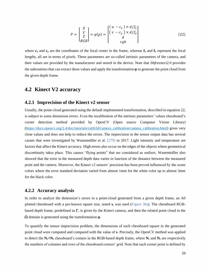
59
𝑃 = [
𝑋𝑌𝑍𝑅𝐺𝐵
] = 𝜑(𝑝) =
[ ( 𝑢 − 𝑐𝑥 ) × 𝑑/𝑓𝑥( 𝑣 − 𝑐𝑦 ) × 𝑑/𝑓𝑦
𝑑𝑟𝑔𝑏 ]
(22)
where cx and cy are the coordinates of the focal center in the frame, whereas fx and fy represent the focal
lengths, all are in terms of pixels. These parameters are so-called intrinsic parameters of the camera, and
their values are provided by the manufacturer and stored in the device. Note that libfreenect2.0 provides
the subroutines that can extract these values and apply the transformation to generate the point cloud from
the given depth frame.
4.2 Kinect V2 accuracy
4.2.1 Imprecision of the Kinect v2 sensor
Usually, the point-cloud generated using the default implemented transformation, described in equation 22,
is subject to some dimension errors. Even the recalibration of the intrinsic parameters’ values chessboard’s
corner detection method provided by OpenCV (Open source Computer Vision Library)
(https://docs.opencv.org/2.4/doc/tutorials/calib3d/camera_calibration/camera_calibration.html) gives very
close values and does not help to reduce the errors. The imprecision in the sensor output data has several
causes that were investigated by Wasenmüller et al. [279] in 2017. Light intensity and temperature are
factors that affect the Kinect accuracy. High errors also occur on the edges of the objects where geometrical
discontinuity takes place. This causes “flying points” that are considered as outliers. Wasenmüller also
showed that the error in the measured depth data varies in function of the distance between the measured
point and the camera. Moreover, the Kinect v2 sensors’ precision has been proved influenced by the scene
colors where the error standard deviation varied from almost 1mm for the white color up to almost 3mm
for the black color.
4.2.2 Accuracy analysis
In order to analyze the dimension’s errors in a point-cloud generated from a given depth frame, an A0
plotted chessboard with a pre-known square size, noted s, was used (Figure 36a). The chessboard RGB-
based depth frame, predefined as , is given by the Kinect camera, and then the related point cloud in the
domain is generated using the transformation .
To quantify the sensor imprecision problem, the dimensions of each chessboard square in the generated
point cloud were computed and compared with the value of s. Precisely, the OpenCV method was applied
to detect the Nc×Nr chessboard’s corners in the RGB-based depth frame, where Nc and Nr are respectively
the numbers of columns and rows of the chessboard corners’ grid. Note that each corner point is defined by

60
its column index i[0, Nc-1] and row index j[0, Nr-1]. Since the corners 2D coordinates (u, v) given by
the OpenCV method are not necessarily integer values, the depth value of each of these points is estimated
from the depth frame by applying the bilinear interpolation. Let c be the group of corner points extracted
from the frame, and c be the group of corner points in the 3D space. c and c . For each corner
point pci,j c, the corresponding 3D point Pc
i,j c is given as follows:
𝑃𝑖,𝑗𝑐 = 𝜑(𝑝𝑖,𝑗
𝑐 ) (23)
In addition, after calculating the position of each corner point in the 3D space, the Euclidean distances
between each point Pi,j and its adjacent points, 𝑑𝑖,𝑗ℎ1, 𝑑𝑖,𝑗
𝑣1, 𝑑𝑖,𝑗ℎ2 and 𝑑𝑖,𝑗
𝑣2, as shown in Figure 36b:
Figure 36. A0 chessboard used for the quantification of the Kinect's imprecision (a) and dimensions used to calculate
the errors assigned to the point Pci,j within the A0 chessboard (b).
Knowing already the chessboard actual square size s, absolute errors of these dimensions can be simply
found as follows:
{
𝑒𝑖,𝑗ℎ1 = |𝑑𝑖,𝑗
ℎ1 − 𝑠|
𝑒𝑖,𝑗𝑣1 = |𝑑𝑖,𝑗
𝑣1 − 𝑠|
𝑒𝑖,𝑗ℎ2 = |𝑑𝑖,𝑗
ℎ2 − 𝑠|
𝑒𝑖,𝑗𝑣2 = |𝑑𝑖,𝑗
𝑣2 − 𝑠|
(24)
Then, the absolute horizontal and vertical errors assigned to each corner point are considered as the average
of the 2 horizontal errors and the 2 vertical errors respectively as follows:
{
𝑒𝑖,𝑗ℎ =
𝑒𝑖,𝑗ℎ1 + 𝑒𝑖,𝑗
ℎ2
2
𝑒𝑖,𝑗𝑣 =
𝑒𝑖,𝑗𝑣1 + 𝑒𝑖,𝑗
𝑣2
2
(25)
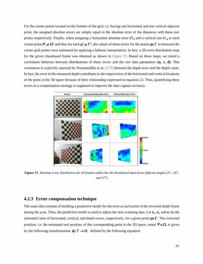
61
For the corner points located on the frontier of the grid, i.e. having one horizontal and one vertical adjacent
point, the assigned absolute errors are simply equal to the absolute error of the distances with these two
points respectively. Finally, when assigning a horizontal absolute error ehi,j and a vertical one ev
i,j to each
corner point Pci,jc and thus for each pc
i,jc, the values of these errors for the points p in-between the
corner grid points were estimated by applying a bilinear interpolation. In fact, a 2D error distribution map
for the given chessboard frame was obtained as shown in Figure 37. Based on these maps, we noted a
correlation behavior between distributions of these errors and the raw data parameters (u, v, d). This
correlation is explicitly reported by Wasenmüller et al. [279] between the depth error and the depth value.
In fact, the error in the measured depth contributes to the imprecision of the horizontal and vertical locations
of the point in the 3D space because of their relationship expressed in equation 22. Thus, quantifying these
errors in a compensation strategy is supposed to improve the data capture accuracy.
Figure 37. Absolute error distribution for all frames within the A0 chessboard taken from different angles (3°, -26°,
and 37°)
4.2.3 Error compensation technique
The main idea consists of building a predictive model for the error at each point of the received depth frame
during the scan. Then, the predictive model is used to adjust the new scanning data. Let ex, ey, and ez be the
estimated rates of horizontal, vertical, and depth errors, respectively, for a given point p. The corrected
position, i.e. the estimated real position, of the corresponding point in the 3D space, noted �� , is given
by the following transformation ��: → defined by the following equation:

62
�� = [
������𝑅𝐺��
] = ��(𝑝) =
[ ( 𝑢 − 𝑐𝑥 ) × (
𝑑
𝑓𝑥) × (1 − 𝑒𝑥)
( 𝑣 − 𝑐𝑦 ) × (𝑑
𝑓𝑥) × (1 − 𝑒𝑦)
𝑑 × (1 − 𝑒𝑧)𝑟𝑔𝑏 ]
(26)
This transformation can also be rewritten as follow:
��(𝑝, 휀) = (𝐼 − 휀). 𝜑(𝑝) (27)
where I is the identity matrix and is the error rate matrix defined as follows:
휀 = [
𝑒𝑥 00 𝑒𝑦
0 00 0
0 00 0
𝑒𝑧 00 0
] (28)
For each point p and its corresponding measured point P obtained by applying the transformation
, if the corresponding estimated real position �� is given, so the error rate matrix can be calculated
by the following equation:
휀 = (𝑃, ��) with (𝑃, ��):
{
𝑒𝑥 =
𝑋 – ��
𝑋
𝑒𝑦 =𝑌 – ��
𝑌
𝑒𝑧 =𝑍 – ��
𝑍
(29)
The predictive model of the error rate matrix for a given point p is defined by the following
equation:
휀 = 𝐿𝑅(𝑝) (30)
where LR stands for the “Linear Regression” model. When obtaining this predictive model, the 3D
positions for all captured points were adjusted using equation 27.
4.2.4 The learning database of the error Compensation technique
To build the predictive model, a learning database is needed. Thus, the real position ��𝐜 should be
estimated within the learning database. A program was developed and executed automatically to get the
frame of the chessboard, detects its corners, and estimates the real position in real-time. For each sensor,
the learning database is created from around 50 frames that were taken while moving the sensor and varying

63
the distance between it and the chessboard in a range between 50cm and 100cm. These frames were taken
after preheating of each sensor for more than 25 minutes, as recommended by Wasenmüller et al. [279] in
order to stabilize the errors by reducing their standard deviation. All data from a single sensor are grouped
into one learning database for applying the linear regression model.
Given the real square size s of the chessboard and the focal center is the center of the transformations from
to , to estimate the real position of the corner point in the space, it is necessary to determine the location
of the focal center with respect to the chessboard corners’ grid. Let c = [cx cy dc rgbc]T be the
focal center. Whereas cx and cy are constant decimal values given for each Kinect camera by the
manufacturer, its depth value dc can be found by bilinear interpolation of the depth frame. The
corresponding point in the 3D space is C = [Xc Yc Zc RGBc]T . Let ic and jc be the column and the
row indexes of the focal center in the chessboard corners’ grid. Since c is located in between the points of
the grid, ic and jc are decimal values. In fact, c is located inside the quadrilateral formed by the following
group of corner points = {𝐩𝐤,𝐥; 𝐩𝐤+𝟏,𝐥 ; 𝐩𝐤+𝟏,𝐥+𝟏 ; 𝐩𝐤,𝐥+𝟏} 𝐜
. Therefore ic[ 𝒌, 𝒌 + 𝟏 ] and
jc[𝒍, 𝒍 + 𝟏]. These two decimal indexes can be estimated by the following equation:
{
𝑖𝑐 = 𝑘 + 𝑑ℎ1
𝑑ℎ1 + 𝑑ℎ2
𝑗𝑐 = 𝑙 + 𝑑𝑣1
𝑑𝑣1 + 𝑑𝑣2
(31)
Figure 38. (a) example of a random chessboard frame received from Kinect sensor and (b) chessboard dimensions
in the domain
where dh1, dh2, dv1, and dv2 (in pixels) are, as shown in Figure 38a, the dimensions between the focal center
and the intersection between the side segments of the quadrilateral with the horizontal and vertical axes
of the chessboard having the direction vectors �� and �� respectively. These direction vectors are estimated
as follows:

64
�� =𝑢1 + 𝑢2
‖𝑢1 + 𝑢2 ‖ ; 𝑣 =
𝑣1 + 𝑣2
‖𝑣1 + 𝑣2 ‖ (32)
Hence, after estimating the location of the focal center in the grid, the estimation of the real position of each
corner point becomes possible. This is done first in the coordinate system having C as the origin and the
horizontal and vertical axes of the chessboard as the X and Y axes respectively (Figure 38b). This domain
is noted and the point in this domain corresponding to the corner point pci,j c will be noted ��𝐢,𝐣
𝐜 , and
can be found using the transformation defined �� : → as follows:
��𝑖,𝑗𝑐 =
[ ��𝑖,𝑗𝑐
��𝑖,𝑗𝑐
��𝑖,𝑘𝑐
𝑅𝐺��𝑖,𝑗𝑐]
= ��(𝑝𝑖,𝑗𝑐 ) = [
𝑠 × (𝑖 − 𝑖𝑐)
𝑠 × (𝑗 − 𝑗𝑐)
0𝑟𝑔𝑏
] (33)
Equation 33 shows that the point ��𝒊,𝒋𝒄 represents the estimated real position of the corner (i,j) relative to
the focal center. Then, from the point ��𝒊,𝒋𝒄 we may estimate the position of the point ��𝒊,𝒋
𝒄 in the domain
by applying a transformation 𝝋∗: → defined by the following equation:
P = 𝜑∗(��) = 𝑅 × �� + 𝐶 (34)
where R is the rotation matrix calculated using the Single Value Decomposition (SVD)-based method to
align the points ��𝒊,𝒋 with the points 𝑷𝒊,𝒋, considering 𝑪 as the center of the former points set, and C as the
center of the latter one. Finally, the real position in the camera 3D domain of each corner point pci,j c
can be estimated using the following formulation:
��𝑖,𝑗𝑐 = 𝜑∗ ∘ �� (𝑝𝑖,𝑗
𝑐 ) (35)
Having the measured position Pci,j (Eq. 23) and the estimated correct position ��𝐢,𝐣
𝐜 (Eq. 35) of a corner point
pci,j, the error can be calculated using equation 29.
4.3 The 3D-scanning platform
4.3.1 System architecture
Our proposed 3D scanning system includes four RGB-Depth Kinects v2 cameras (Figure 39a) mounted on
a mobile mechanical structure allowing to adjust the height of each camera according to the size of the
involved patient. The physical dimension of the space of interest within the 3S scanning system was set up
as 1.5m in the vertical and horizontal planes (Figure 39b). Since the minimum range of the Kinect sensor
is 50cm, we chose to place each sensor at 75 cm away from the center so it can detect the scanned limb

65
with a minimum safety margin of around 17 cm at each side for a transfemoral amputation case. Note that
the average circumference of a human thigh is equal to around 51 cm [280], which is equivalent to a
diameter of around 16 cm.
The four Kinect v2.0 sensors are connected simultaneously to the same workstation. Normally, using the
standard API of the Kinect cameras offered by Microsoft, Kinect SDK 2, it is not possible to use multiple
sensors on one PC: Sensor Acquisition and Startup Kinect for Windows supports one sensor, which is called
the default sensor. That’s why many Kinect-fusion projects found in the literature use the Client-Server
configuration where each sensor is connected to one client PC, and each of these clients is connected to the
server PC using Transmission Control Protocol/Internet Protocol” (TCP/IP) protocol within an Ethernet
network [266, 281-283]. To bypass this limitation, we use, instead of the default SDK, an available open-
source library libfreenect2.0 which uses the libusb driver. Despite the fact that it does not provide many
functions and features provided by the standard API, this package makes it possible for one workstation to
communicate with multiple Kinect v2 sensors.
Figure 39. The proposed 3D scanning platform with four RGB-Depth Kinects v2 cameras and mobile supports (a)
and the physical dimension of the space of interest within the 3D scanning system (b).
The developed system workflow is shown in Figure 40. Each sensor collects data from one side of the
scanned object and generates two types of raw data: the depth frame of 512×424 pixels in millimeters, and
a 1920×1080 pixels RGB-based frame for color data. From each raw dataset, a 3D point cloud is generated
and corrected with an error compensation algorithm that estimates the error on each point. Then, each point
set is filtered to remove the outliers. To align the four filtered point sets together, the extrinsic parameters
of each camera should be calculated, so that all point sets can be transformed into the same coordinate
system and merged into a globally consistent model. To achieve this objective, a multi-set registration
method was proposed. Finally, once the fused point cloud is obtained, it is used in a 3D surface
reconstruction process to create the final 3D model.

66
Figure 40. 3D scanning system workflow from data fusion to 3D surface reconstruction: (a) the four acquired point-
clouds; (b) filtered point-clouds; (c) aligned point-clouds using multi-set registration method; (d) reconstructed 3D
surface of the limb
4.3.2 Multi-set registration problem
Captured point cloud from depth cameras suffers from the well-known artifact related to “flying points”
[284], which occurs mainly close to depth discontinuities (Figure 41a) and is considered as outliers. To
remove them, a statistical outlier removal algorithm was applied to each generated point-cloud,
implemented using the open-source library PCL 1.9.1 [285].
Figure 41. Illustration of outlier removal from the point cloud of a scanned white tube (a) and the rigid multi-set
registration process for four point-clouds (b).
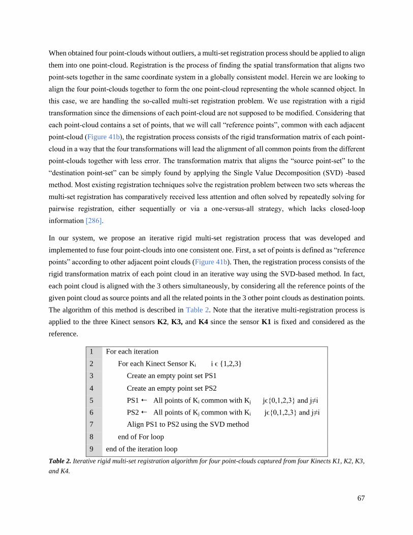
67
When obtained four point-clouds without outliers, a multi-set registration process should be applied to align
them into one point-cloud. Registration is the process of finding the spatial transformation that aligns two
point-sets together in the same coordinate system in a globally consistent model. Herein we are looking to
align the four point-clouds together to form the one point-cloud representing the whole scanned object. In
this case, we are handling the so-called multi-set registration problem. We use registration with a rigid
transformation since the dimensions of each point-cloud are not supposed to be modified. Considering that
each point-cloud contains a set of points, that we will call “reference points”, common with each adjacent
point-cloud (Figure 41b), the registration process consists of the rigid transformation matrix of each point-
cloud in a way that the four transformations will lead the alignment of all common points from the different
point-clouds together with less error. The transformation matrix that aligns the “source point-set” to the
“destination point-set” can be simply found by applying the Single Value Decomposition (SVD) -based
method. Most existing registration techniques solve the registration problem between two sets whereas the
multi-set registration has comparatively received less attention and often solved by repeatedly solving for
pairwise registration, either sequentially or via a one-versus-all strategy, which lacks closed-loop
information [286].
In our system, we propose an iterative rigid multi-set registration process that was developed and
implemented to fuse four point-clouds into one consistent one. First, a set of points is defined as “reference
points” according to other adjacent point clouds (Figure 41b). Then, the registration process consists of the
rigid transformation matrix of each point cloud in an iterative way using the SVD-based method. In fact,
each point cloud is aligned with the 3 others simultaneously, by considering all the reference points of the
given point cloud as source points and all the related points in the 3 other point clouds as destination points.
The algorithm of this method is described in Table 2. Note that the iterative multi-registration process is
applied to the three Kinect sensors K2, K3, and K4 since the sensor K1 is fixed and considered as the
reference.
1 For each iteration
2 For each Kinect Sensor Ki i ϵ {1,2,3}
3 Create an empty point set PS1
4 Create an empty point set PS2
5 PS1 All points of Ki common with Kj jϵ{0,1,2,3} and j≠i
6 PS2 All points of Kj common with Ki jϵ{0,1,2,3} and j≠i
7 Align PS1 to PS2 using the SVD method
8 end of For loop
9 end of the iteration loop
Table 2. Iterative rigid multi-set registration algorithm for four point-clouds captured from four Kinects K1, K2, K3,
and K4.

68
4.3.3 3D reconstruction
The 3D surface reconstruction method aims to reconstruct the final 3D surface from the fused point cloud.
In fact, the problem of surface reconstruction from a point sample is ill-defined: because the points only
provide a sample of the surface, we cannot determine with exact certainty how the surface behaves between
the points. Besides, for real-world data-sets, we also must handle outliers and small errors in the points'
locations that do not sample the surface perfectly. To overcome these obstacles, a scale-space 3D
reconstruction algorithm has been developed [287]. This method is already provided by the open-source
CGAL library. However, one main drawback of this method is its inability to close the holes that may
appear in the point-cloud (Figure 42a) due, e.g., outlier removal filter or occlusion during. An alternative
method may be the Poisson algorithm also provided by CGAL library. This contouring algorithm always
extracts a closed surface mesh and hence can fill the holes, but on the other hand, it does not provide any
means to trade data fitting for smoothness so it is unable to handle with noisy point-cloud (Figure 42a).
Figure 42. 3D reconstruction problem: (a) using Poisson or scale-space; (b) the process using both Poisson and
scale-space algorithm
Hence, we use a surface reconstruction combining these two algorithms. As shown in Figure 42b, the
Poisson algorithm is first applied to generate a closed 3D surface. The points of this surface mesh are
extracted to form a second point-cloud to be used as input to the scale-space algorithm. The surface
produced by this process is closed thanks to the former algorithm, and smooth thanks to the latter one.

69
4.4 Application
4.4.1 Technical implementation
The main program was developed using C++ with a graphical user interface created using VS2019
Windows Form Application (.net framework). All developed codes were combined into one package, called
OpenMKS (Multi-Kinect Scan) which is open source free software available on the following link
(https://github.com/abbassb88/OpenMKS). Since the default driver of the Kinect v2 camera does not
support natively multiple cameras on the same workstation, OpenMKS requires installing another driver,
libusb 3.0, which is required for the libfreenect2.0 library. The graphical user interface of OpenMKS is
shown in Figure 43.
Note that the 3D acquisition from multiple Kinect v2 sensors, error compensation, outlier removal, multi-
set registration, 3D surface reconstruction, as well as an implemented point-cloud up-sampling tool are all
included in this package. The point-cloud up-sampling procedure allows the user to up-sample the depth-
frame data (and so the point cloud) by N times, i.e. increasing the resolution of the depth-frame from
512×424 to (512×N) × (424×N), where N is an integer representing the up-sampling factor given by the
user. This has been done by estimating the depth values of the new pixels introduced in between the original
ones by simply applying bilinear interpolation. This up-sampling feature was useful during the multi-set
registration step where a higher resolution frame was necessary for better detection of the chessboard
corners using OpenCV.
Figure 43. Graphical User Interface of OpenMKS

70
4.4.2 Accuracy evaluation
A testing database was created consisting of three chessboard frames where the sensor is placed at 60cm,
75cm, and 90cm far from the chessboard respectively. Each of these frames was taken and visualized before
and after the introduction of the error compensation system. Then, the absolute errors of the chessboard
dimensions at each case were computed and visualized. The statistical t-test was used for comparison
purposes.
To evaluate the accuracy of our proposed iterative rigid multi-set registration process, a comparison with a
traditional sequential registration method [288-289] was performed on a box (length =30cm, width = 30cm,
and height =70cm) with a chessboard on each of its sides as “registration object” (Figure 44a).
Besides, the error compensation strategy was applied on three cylindrical objects of diameters 10cm, 16cm,
and 21cm mimicking the human residual limb to quantify its accuracy (Figure 44b). The 3D models
generated by the scan were compared with a reference 3D cylindrical object having the physical dimensions
of the scanned objects. The comparison was performed using MeshLab, an open-source system for
processing 3D triangular meshes. The scan and the reference models were aligned together using the
Iterative Closest Point (ICP) method, and then Hausdorff distance has been used to compute the differences
between the two meshes. The reference cylindrical objects were generated by a simple C++ code that writes
it in binary STL format.
Figure 44. (a) The calibration box, (b) the three cylindrical test objects
4.5 Results
4.5.1 Accuracy of the error compensation strategy
The integration of the error compensation strategy leads to reduce the reconstruction error according to the
case without error compensation. Figure 45, Figure 46, Figure 47, and Figure 48 show these results on the
three tested chessboard frames (i.e. sensor is placed at 60cm, 75cm, and 90cm far from the chessboard) for
the four Kinect sensors respectively.

71
Figure 45. Dimensions error patterns in the horizontal and vertical planes for the three tested chessboard frames
without and with error compensation for the Kinect sensor K1 (AE: Absolute Error).
Figure 46. Dimensions error patterns in the horizontal and vertical planes for the three tested chessboard frames
without and with error compensation for the Kinect sensor K2 (AE: Absolute Error).
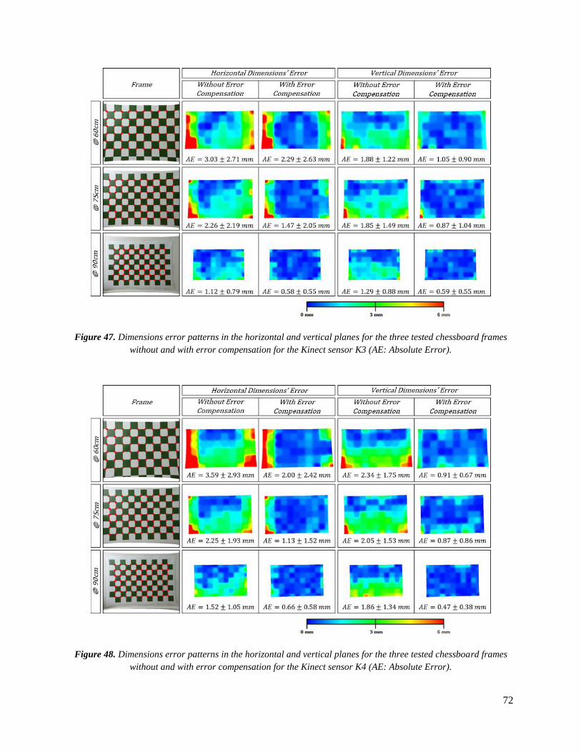
72
Figure 47. Dimensions error patterns in the horizontal and vertical planes for the three tested chessboard frames
without and with error compensation for the Kinect sensor K3 (AE: Absolute Error).
Figure 48. Dimensions error patterns in the horizontal and vertical planes for the three tested chessboard frames
without and with error compensation for the Kinect sensor K4 (AE: Absolute Error).

73
It is interesting to note that when applying the error compensation model, the reconstruction errors were
significantly reduced (t-test, p < 0.005). The grand mean absolute errors in both horizontal and vertical
planes were reduced from 1.69±0.38 mm to 1.10±0.36 mm, from 1.84±0.63 mm to 1.05±0.49 mm, from
1.91±0.63 mm to 1.14±0.59 mm, from 2.10±0.35 mm to 1.42±0.69 mm for the Kinects K1, K2, K3, and
K4 respectively.
Regarding the reconstruction without error compensation, high errors (around 6mm) mostly occurred at the
corners. Moreover, the 60cm- and 75cm frames lead to higher errors (around 6mm) than the case of the
90cm frame (around 3mm). This behavior is common for all four Kinect cameras. To focus the analysis on
these regions of interest, the absolute dimension errors were computed for the frontiers’ points of the
chessboards. The results are shown in Table 3 for the Kinects K1, K2, K3, and K4 respectively. The
statistical t-test (p < 0.005) confirmed a significant reduction of error in these regions of interest. For these
regions of interest reconstructed without error compensation, the maximal error of 5.01 ± 3.52 mm was
noted for the Kinect sensor K4 with a 60cm-case chessboard. The minimal error is around 1.35 ± 1.02 mm
for the Kinect sensor K3 with a 90cm-case chessboard.
Table 3. Dimensions’ errors of the edge points of the three tested chessboards in horizontal and vertical planes without
and with error compensation for all Kinect sensors (K1, K2, K3, AND K4)
When applying the error compensation, these errors were significantly reduced. In the horizontal plane, the
minimal error is around 0.85 ± 0.69 mm for the Kinect sensor K3 with a 90cm-case chessboard. The
maximal error is around 3.49 ± 3.22 mm for the Kinect sensor K3 with a 60cm-case chessboard. In the
vertical plane, the minimal error is around 0.60 ± 0.47 mm for the Kinect sensor K4 with a 90cm-case
Kinect Frame
Horizontal Dimensions’ Error
Vertical Dimensions’ Error
Without Error
Compensation
With Error
Compensation
Without Error
Compensation
With Error
Compensation
K1 @ 60cm 2.61 ± 1.78 mm 1.63 ± 1.07 mm 1.77 ± 0.96 mm 1.04 ± 0.59 mm
@ 75cm 3.77 ± 2.92 mm 2.70 ± 2.45 mm 2.43 ± 1.60 mm 1.14 ± 0.81 mm
@ 90cm 1.87 ± 1.26 mm 1.14 ± 1.21 mm 1.54 ± 1.05 mm 0.61 ± 0.46 mm
K2 @ 60cm 2.73 ± 1.97 mm 1.78 ± 1.84 mm 1.84 ± 0.95 mm 1.17 ± 1.03 mm
@ 75cm 4.43 ± 3.04 mm 3.35 ± 2.99 mm 2.53 ± 1.36 mm 1.25 ± 0.97 mm
@ 90cm 2.09 ± 1.34 mm 1.34 ± 1.21 mm 1.49 ± 1.02 mm 0.72 ± 0.53 mm
K3 @ 60cm 4.23 ± 3.29 mm 3.49 ± 3.22 mm 2.38 ± 1.47 mm 1.55 ± 1.08 mm
@ 75cm 3.29 ± 2.98 mm 2.45 ± 2.82 mm 2.49 ± 1.98 mm 1.43 ± 1.41 mm
@ 90cm 1.35 ± 1.02 mm 0.85 ± 0.69 mm 1.45 ± 1.16 mm 0.87 ± 0.73 mm
K4 @ 60cm 5.01 ± 3.52 mm 3.15 ± 3.00 mm 2.97 ± 2.13 mm 1.23 ± 0.82 mm
@ 75cm 3.27 ± 2.50 mm 1.89 ± 2.10 mm 2.51 ± 2.01 mm 1.22 ± 1.15 mm
@ 90cm 1.88 ± 1.28 mm 0.93 ± 0.72 mm 2.17 ± 1.55 mm 0.60 ± 0.47 mm

74
chessboard. The maximal error is around 1.55 ± 1.08 mm for the Kinect sensor K3 with a 60cm-case
chessboard. Note that the errors are small in the vertical plane according to those in the horizontal plane.
In addition, the reconstruction of three 3D cylindrical objects (diameters of 10cm, 16cm, and 21cm
respectively) mimicking the geometry of the residual limb (diameter of around 16mm) has a smaller error
range when applying the error compensation strategy (Figure 49). The root-mean-square error for the 10cm
tube has been reduced from 1.643mm to 1.254 mm (23.68%), from 2.738 mm to 1.659 mm (39.41%) for
the 16cm tube, and from 2.556 mm to 1.774 mm (30.59%) for the 21cm tube. The maximal errors reduce
from 6.03 mm to 3.73 mm, from 8.1 mm to 5.93 mm, from 6.99 mm to 5.465 mm for the 10cm, 16cm, and
21cm tubes respectively.
Figure 49. Dimensions error patterns for the three tubes reconstructed using sensor fusion without and with
applying the error compensation technique.

75
4.5.2 Speed of the scanning process
The recorded average time for a complete scan is 25.4 ± 2.5 seconds (Figure 50). This time has been
recorded on an HP Intel® Core™ i7-7700HQ CPU @ 2.80GHz 16GB RAM workstation. The first 12.6 ±
2.3 seconds were spent for quasi-simultaneous data collection from the four sensors and point-cloud
generations. Then, the outliers’ removal takes around 0.3 seconds. Finally, the 3D surface reconstruction,
which uses two algorithms successively, takes around 12.5 seconds.
Figure 50. Average timeline of the full scanning process.
4.5.3 Accuracy of the multiple point cloud registration process
Our iterative rigid multi-set registration process was compared to the conventional sequential approach.
Obtained results showed a reduction of error with our approach (Figure 51 and Table 4).
Figure 51. steps and visual reconstruction outcome of the multi-set registration.
Note that the Euclidean distance between the pair of reference points was quantified. In the ideal case, this
distance should be null for each pair. Thus, the mean errors reduce from 5.298 mm to 2.226 mm (~ 58 %)
for our iterative registration approach according to the sequential registration approach without error

76
compensation. Importantly, when applying the error compensation, this error is smaller and reaches a value
of 2.064 mm (reduction of ~ 61%).
Registration Method Mean Error
(mm)
Minimum Error
(mm)
Maximum Error
(mm)
Sequential registration 5.298 0.595 17.365
Iterative registration 2.226 0.563 4.363
Iterative registration + Error compensation 2.064 0.133 3.921
Table 4. Summary of the registration errors for different registration schemes
4.6 Discussions
A low-cost, rapid, and accurate 3D scanning system for the residual limb has attracted the attention of many
researchers in the last two decades. Since the prosthetic design is customized with the unique geometry and
mechanical function of a patient’s stump, such a system will allow automatic prosthetic CAD systems to
be developed for maximizing the benefit of amputee patients. Detailed and expensive imaging modalities
such as CT or MRI have been investigated as well as other sensing capacities like turning ultrasound
sensors, portable low-cost scanners or even portable low-cost RGB-Depth cameras [60, 104, 187]. Note
that CT or MRI modalities are more suitable for the design of osseointegrated prosthetic implants while
other surface-based sensing techniques are more applicable for conventional socket-stump prosthesis [290].
Portable optical scanners [70, 96-98], as well as ultrasound scanning [106-111], have been used to
reconstruct the 3D geometrical model of the stump. However, the reported scanning time of these
techniques was 2 to 3 minutes, which is a long period that will increase the error risks due to muscle
contractions and involuntary limb displacements during the scan. Multiple visual sensor fusion has been
proposed in the literature but only a study deals with the prosthetic application [291]. However, there is no
reported evaluation for the accuracy of such a complex fusion system. The objective of our present work
was to complete the literature about this subject by proposing a systematic evaluation process to quantify
the imprecision of multiple visual sensor fusion for prosthetic applications. Then, an error compensation
strategy was proposed and evaluated leading to reduce 40% of reconstruction error for stump-like
geometries. Finally, all sensing and processing procedures were integrated into an open-access library,
called OpenMKS. This library is freely shared to facilitate new contributions in the field.
A fixed scanning platform with four sensors has been proposed in this study in order to capture the four
sides of the stump simultaneously. This fact will eliminate the risks of model deviation because of the
involuntary movements of the limb during the acquisition, as witnessed in the case of the portable scanner
[71] or rotatable sensors [109]. A compensation camera has been proposed to track these movements and
compensate the related errors [109]..

77
The fusion of heterogeneous data and sensors has been intensively studied in many fields such as
multimedia or medical applications [292-295]. In particular, sensor fusion has become a potential solution
for the 3D reconstruction of complex objects such as human body structures [291]. Within the context of
the prosthetic design application, the reconstruction speed plays an important role to reduce the medial cost,
increase the comfort of the involved patients, and reduce the potential mesh distortion due to the stump
small movements. Our proposed fusion scheme of four Kinect sensors and specific processing procedures
leads to an effective scanning duration (around 25.4 ± 2.5 seconds) for each full acquisition and
reconstruction process. Note that the most critical part of this process is the data-collection from the
patient’s limb costing around 12.6 seconds. This is a very short period compared to the other works (2-3
minutes).
The use of portable and low-cost Kinect sensor (v1 and v2) opens new opportunities for a rapid and low-
cost 3D scanning system. However, the capacity of connecting multiple sensors into a single workstation
remains a technological challenge. The main reason relates to the USB 3.0 ports, to which the multiple
sensors are connected, which are sharing the same USB controller that is not able to support the bandwidth
of more than one sensor. Indeed, the default Kinect API provided by Microsoft does not support more than
one sensor on each PC. In fact, this issue is a runtime and hardware problem because of the unavailable
USB3 bandwidth for multiple sensors. That’s why many researchers used the client-server configuration to
deal with multiple sensors simultaneously [266, 281-283]. In our present work, we proposed a more
effective where multiple Kinect v2 sensors to be connected to a single PC in a straightforward way and thus
is more suitable for a complete rapid and low-cost 3D scanning system. Furthermore, we decided to make
our library an open-source one. It is expected that this contributes to the promotion of this solution within
the community and speed up the development of new effective and innovative solutions for medical and
industrial purposes.
Regarding the accuracy of scanning capacity with multiple Kinect sensors, an error compensation strategy
was proposed to correct the raw measurements coming from each sensor. Our proposed solution allows an
important reduction level of the 3D geometrical reconstruction error. In fact, a reduction of root-square-
mean error about 23% to 40% is reached for stump-like geometries while the peak error was reduced by
about 21% to 38%. The absolute error values are between 1.2mm and 1.8mm which are 0.8% to 1.3%
relative to the scanned object diameter. These results are competitive according to earlier recent error
compensation works, where the obtained average error is 2.75mm using the ultrasound scan [190], 1.4% to
4% and may sometimes reach 8% using the image processing technique [99], 1.4% to 2% using a portable
scanner [98]. Note that the linear regression model was used in our error compensation strategy. The
polynomial regression system with second and third-order was also implemented and evaluated. However,
unsatisfied outcomes were obtained for this system. One of the possible reasons relates to the unexpected
tail behavior of the polynomials. These tails tend to wiggle around, making the polynomials bad for

78
extrapolation and even for interpolation where input values get closer to the end of the learning data. One
of the possible future works can be the study and evaluation of more complex machine learning models
such as deep learning [296]. Moreover, the optimal scanning zone, i.e. the optimal position of the scanned
object relative to the sensors, may be also investigated in future work to minimize the errors, especially the
peak error (located mainly at the bottom half of the scanned object) that is still high (3.7mm to 5.9mm).
Two assumptions were performed in our error compensation strategy. The first one deals with the
assumption of the correct direction of the measured chessboard and the second one is the correct location
of the depth-frame focal center within the measured chessboard. These assumptions were made because of
unavailable information to compute them from the raw data. Hence, future work may focus on increasing
the accuracy of the errors’ model by improving the estimation of the correct position of the chessboard in
the camera 3D space. For the moment, to reduce the effect of the first assumption, we tried to keep the
camera horizontal and parallel to the chessboard plane as possible while taking the multiple frames for the
learning database generation. Finally, in this present study, only 3D cylindrical objects mimicking the
geometry of the residual limb were used and evaluated. Further investigations should be carried out to
confirm the findings and enhance the validation of the proposed fusion scheme and error compensation
strategy on the lower residual limb geometries. Moreover, the use of a visual camera like Kinect leads to
the capture of only external geometries. In the context of a complete computer-aided prosthetic design
system, internal geometries like bony structures need to be also reconstructed. Consequently, a statistical
shape modeling method or machine learning method should be investigated to study this relationship toward
an automatic generation of internal structures from external information.

79
Parametric Digital Design of the
Prosthetic Socket
The third step of the socket CAD workflow is discussed in this chapter. A novel numerical design method
for the prosthetic socket is proposed. This approach is based on the calculation of the stump-socket
interaction to predict the pressure distribution on the contact interface as a numerical indicator of the fit-
quality. Whereas a node-to-surface discrete contact formulation has been implemented and used to validate
our model compared to FE outcomes (chapter 3), a remarkable decrease in the calculation speed has been
witnessed when it is introduced in the simulation. In fact, a discrete contact detection formulation is very
simple and does not require high computational resources, but requires small time-steps for the sake of
stability which slows down the simulation. On the other side, a fast calculation is favorable to an interactive
design process with instant numerical feedback. For this purpose, an inverse calculation of the stump-socket
interaction is proposed in this study to eliminate the need for the direct contact formulation, and
consequently speed-up the process. This approach provides mechanical constraints along with other quality-
related constraints that will numerically define the shape of the well-fit socket. Thus, it consists of a
Constraint Satisfaction Problem (CSP) where an instant calculation is performed to check the satisfaction
level and given as instant feedback to guide the designer. This CAD system has been implemented along
with a user-friendly interface and parametric design tools and evaluated by comparing its outcomes with
the outputs of FE simulations
5.1 Computer-aided parametric socket design workflow
A computer-aided parametric socket design workflow was developed and shown in Figure 52. The design
socket process starts from an acquisition of a 3D geometrical model of the patient’s residual limb. Then, an
inverse calculation process of the stump-socket interaction was performed. This process consists of
determining the shape of the rigid contact surface of the socket from both the pressures applied to the
stump’s surface, considered equivalent to the contact pressure and the stump’s surface deformation. During
this interactive process, local pressures are applied to the surface to describe the contact pressure
distribution. The pressures are parametrically applied and they are subject to numerical constraints to ensure
that they are equivalent to contact pressures along with other constraints related to the socket design quality.
Numerical feedback from the dynamic soft-tissue deformation process performed in function of the applied
pressures is used to ensure that the applied pressures satisfy all prescribed constraints. Finally, the rigid

80
contact surface is reconstructed from the deformed surface of the stump, and a thickness is added to generate
the socket model.
Figure 52. The proposed computer-aided parametric socket design workflow to automatically generate a patient-
specific virtual socket prototype.
To provide the soft tissue deformation feedback during the parametric and interactive design process, a
Mass-Spring System with Corrective Springs (MSS-CS) model was used. Which has been described in
Chapter 3. For recall, this model is defined by the following parameters: (soft tissue density), E (soft
tissue elasticity modulus), A (ratio between the edge and face diagonal springs’ stiffnesses), and constants
C and for the corrective springs’ formulation.
5.2 Inverse approach for stump-socket interaction
5.2.1 Theoretical basis
The interaction of the residual limb and the prosthetic socket is a highly dynamic process [297]. However,
for simplification, we will consider the static case of the standing up configuration. In this case, we assume
that the patient’s weight is equally distributed between the two legs. Thus, we consider that the prosthetic
device bears a vertical load that is equal to half of the patient’s weight. Let M be the weight of the patient
in kg, and g the gravitational acceleration, the total force, in terms of Newton, applied by the body to the
prosthetic socket during the standing up posture is expressed by the following equation:
𝐹 𝑆 = 𝑀
2�� = −
𝑀𝑔
2 𝑒 𝑧 (36)

81
The ‘S’ in �� 𝑺 stands for ‘Socket’, and �� 𝒛 is the unit vector of the vertical axis in the Euclidian 3D space.
According to the third law of Newton, the socket is applying to the patient’s body, in this case, the residual
limb, a force 𝐹 𝑅, equal to 𝐹 𝑆 in magnitude, but opposite in direction. Therefore, the force applied by the
socket to the stump is expressed as follows:
𝐹 𝑅 = 𝑀𝑔
2 𝑒 𝑧 (37)
Considering �� 𝑹 the total torque applied by the socket to the residual limb, since the system is in
equilibrium, we consider that the total torque is null. The parameters of the interaction between the socket
and the stump are illustrated in Figure 53.
Figure 53. illustrations of the applied loads by the socket to the stump during the standing up posture (a) and the
force components applied to a single node of the stump’s surface (b).
In a discrete domain where the residuum is represented by a group of nodes, as in the MSS-CS model (that
will be applied in our present study), the total force applied to the stump is equal to the sum of the forces
applied individually to each node. Since the load under investigation is an external load applied to the
surface of the stump, the nodes of interest will be the surface nodes. Let be the domain of the 3D surface
nodes of the stump, N be the number of these nodes, and pi is of these points with i[0, N-1]. The total
force 𝐹 𝑅 can be expressed as follows:
𝐹 𝑅 = ∑ 𝐹 𝑖𝑁−1
𝑖=0
(38)
where �� 𝒊 is the force applied by the socket’s surface to the node pi. As shown in Figure 53a, this force is
the resultant of two forces: the normal contact force �� 𝑪𝒊 , and the tangential static friction force �� 𝒇𝒓
𝒊 as
follows:
𝐹 𝑖 = 𝐹 𝐶𝑖 + 𝐹 𝑓𝑟
𝑖 (39)
Equation 39 can be thus expressed as follows:

82
𝐹 𝑅 = ∑(𝐹 𝐶𝑖 + 𝐹 𝑓𝑟
𝑖 )
𝑁−1
𝑖=0
(40)
We here consider the static friction since the standing up posture is a static case. The static friction is
basically directed in the opposite direction of the applied tangential force. In our case, this friction is the
response to the vertical force �� 𝑹 which makes an angle i with the tangent of the stump surface at each
point pi (Figure 53b). Thus, the frictional norm at pi will be estimated as follows:
𝐹𝑓𝑟𝑖 = 𝜇𝐹𝑓𝑟
𝑖 × 𝑐𝑜𝑠(𝜃𝑖) (41)
where is the friction coefficient constant between the socket and the stump. From equations 37, 39, and
71, we deduce the following expression:
𝐹 𝑅 =
[
∑𝐹𝑐,𝑥𝑖
𝑁
𝑖=0
∑𝐹𝑐,𝑦𝑖
𝑁
𝑖=0
∑𝐹𝑐,𝑧𝑖 + 𝜇𝐹𝑐
𝑖 × cos(𝜃𝑖)
𝑁
𝑖=0 ]
= [
00𝑀𝑔
2
] (42)
where 𝐹𝑐,𝑥𝑖 , 𝐹𝑐,𝑦
𝑖 and 𝐹𝑐,𝑧𝑖 are the components of the 3D vector 𝐹𝑐
𝑖 in the Euclidian space.
The same analogy can be applied to the torque. Each 𝑭𝒄𝒊 applied to pi is creating a torque applied to the
stump with respect to its center of Inertia CI. This individual torque noted �� 𝒊, is expressed as follows:
𝜎 𝑖 = 𝐹 𝑐𝑖 × 𝑃𝑖𝐶𝐼 (43)
The total torque, �� 𝑹, that is a null vector as aforementioned is the sum of the individual torques �� 𝒊 applied
at each point, thus:
𝜎 𝑅 =∑𝜎𝑖
𝑖
=∑(𝐹 𝑐𝑖 × 𝑃𝑖𝐶𝐼 )
𝑖
= 0 (44)
5.2.2 Inverse approach
A. The principle
Let f be the field of 3D vectors representing the force distribution applied to the stump surface. These
forces are assumed to be normal vectors to the surface of the stump since they are supposed to represent
the normal contact forces. To each pi , we assign a force �� 𝑪𝒊 f. this force, supposed equivalent to a

83
contact force with the rigid surface of the stump during the standing up posture, produces a static friction
force 𝑭𝒇𝒓𝒊 as expressed in equation 41, and a torque �� 𝒊 with respect to the stump’s center of inertia as
expressed in equation 43. Given the deformed surface of the stump as a response to the applied forces f,
we consider that these applied forces are equivalent to a contact force with a rigid socket, whose inner
surface morphology is equal to the shape of the stump’s deformed surface and subject to a total force equal
to �� 𝑹 expressed in equation 42 and a total torque �� 𝑹 as expressed in equation 44.
In other terms, to be equivalent to the contact force distribution with a rigid socket during the standing up
posture, an applied force distribution to the stump surface f should respect the equalities shown in
equations 43 and 45. The shape of the socket surface is then equal to the shape of the deformed stump’s
surface.
B. The comfortability
We consider that a socket is comfortable during the prosthetic usage if the applied stresses to the stump
don’t cause pain. Inappropriate pressure distribution can generate many discomforts, and high local
pressures applied for a long time to the skin may cause skin problems. As the relationship between stresses
and discomfort varies for each subject depending on weight, residual muscle tonicity, and lifestyle [77],
identifying pressure threshold values can be the first step to reduce potential discomfort [126]. Many
researchers attempted to measure these thresholds [126-130], however, standard threshold values are not
available yet, especially because they depend dramatically on the status and unique features of the patient
residual tissues.
In the present study, the pain-threshold distribution measured for each stump is assumed to be available.
This pain-threshold distribution is assigned to the stump’s MSS-CS model, translated into maximum force
values, noted 𝑭𝒄,𝒎𝒂𝒙𝒊 assigned to each surface node pi . The comfortability is thus achieved as long as
the following constraint is respected:
𝐹𝑐 𝑖 < 𝐹𝑐, 𝑚𝑎𝑥
𝑖 𝑓𝑜𝑟 𝑎𝑛𝑦 𝑖 ∈ [0, 𝑁 − 1] (45)
C. The stability
Ideally, the socket would transmit forces from the user limb to the prosthesis and vice versa with perfect
efficiency, transferring any movements of the residual limb bone without loss of motion to the prosthetic
limb. However, an inappropriate socket fit may cause instability of the prosthetic device. The instability is
a complex behavior that may include tilting and slipping. Whereas tilting is related to the fact that the soft
tissues between the prosthetic socket and the residual limb bone are not rigid, the slipping behavior is a
translation movement of the socket with respect to the intrinsic bone that occurs when the external forces

84
pulling the prosthetic down exceed the static friction force [298]. Usually, this phenomenon leads to the
“pistoning” [299] that occurs when the residual limb slips up and down inside the prosthetic socket while
walking, and also relates to the friction between the socket and the stump. Therefore, we assume that a
stable socket, that does not exhibit a pistoning behavior, is the one that provides sufficient static friction
against the pulling downforce. The static friction at each surface point pi against a vertical
pushing/pulling force is given in equation 41. The total static friction is the sum of these individual static
frictions, and expressed as follows:
𝐹𝑓𝑟 = ∑ 𝐹𝑓𝑟𝑖
𝑁−1
𝑖=0
= ∑(𝜇𝐹𝑓𝑟𝑖 × 𝑐𝑜𝑠(𝜃𝑖))
𝑁−1
𝑖=0
(46)
Thus, we consider that a stable socket, with no pistoning behavior, is the one that respects the following
constraint:
𝐹𝑓𝑟 ≥ 𝐹𝑓𝑟,𝑚𝑖𝑛 (47)
where 𝑭𝒇𝒓,𝒎𝒊𝒏 is a certain predefined minimum value of the static friction. In the present study, we assume
that the slip of the socket is mainly due to a weak friction force that is not able to resist the weight of the
prosthesis, therefore, 𝑭𝒇𝒓,𝒎𝒊𝒏will be set as the weight of the prosthetic device, which is around 2Kg [297].
D. Summary of the proposed approach
The proposed method consists of finding the shape of the socket inner surface, from a normal pressure
distribution applied to the stump surface along with the deformed geometry of the stump model. The applied
pressure distribution is considered as the equivalent of the contact pressures between the stump and the
well-fit socket to be found. To be so, the applied pressure distribution should respect the four constraints
expressed in equations 42, 44, 45, and 47.
5.3 Interactive parametric design
To easily apply the pressure distribution to the stump’s surface, we developed a parametric tool that allows
the user to apply a local pressure spot in the desired location and with the desired size and magnitude by
simply tuning some parameters. These local pressures are in fact the analogical concept of the local
modifications applied in the conventional socket fabrication method: pressure is applied where the
prosthetist usually removes plaster from the residual limb’s replica to tighten the socket. The overall
pressure distribution is created by applying multiple local pressures where needed. The idea consists of
representing the local pressure distributions using parametric functions. Since the residual limb is a
cylindrical-based shaped object, we chose to use the cylindrical coordinate system to express the parametric
functions (Figure 54).

85
Figure 54. The cylindrical coordinate system for a transtibial residual limb model.
A CAD tool is also created to allow the user to identify the shape of the socket brim. The brim line is also
parametrized by defining some key-points and generated using the spline model.
A. Local pressures
We used the three key-functions shown in Table 5 to build the parametric functions of the local pressures.
These three key functions consist of a co-sinusoidal function, a multiplication of two sigmoid functions,
and a ramp function respectively.
Notation Expression Representation Parameters
COS
𝑓𝐶𝑂𝑆(𝑥)
= {
1
2[1 + cos (
𝜋(𝑥 − 𝑥0)
𝑅𝑥)] 𝑖𝑓 𝑥 ∈ [𝑥0 − 𝑅𝑥, 𝑥0 + 𝑅𝑥]
0 𝑜𝑡ℎ𝑒𝑟𝑤𝑖𝑠𝑒
𝑥0 𝑎𝑛𝑑 𝑅𝑥
SIG 𝑓𝑆𝐼𝐺(𝑥) =1
[1 + 𝑒−𝜆(𝑥−𝑥1)]×
1
[1 + 𝑒𝜆(𝑥−𝑥2)]
𝑥1, 𝑥2 𝑎𝑛𝑑 𝜆
RMP 𝑓𝑅𝑀𝑃(𝑥) =
{
1 𝑖𝑓 𝑥 < 𝑥1(𝑥 − 𝑥2)
(𝑥1 − 𝑥2) 𝑖𝑓 𝑥 ∈ [𝑥1, 𝑥2]
0 𝑖𝑓 𝑥 > 𝑥2
𝑥1 𝑎𝑛𝑑 𝑥2
Table 5. The key-functions used to build the parametric functions of the local pressure distribution.
Again, the pressures are translated into forces because we are dealing with the MSS-CS model consisting
of nodes. Each pi can be represented in the cylindrical system with its cylindrical coordinates

86
(𝝆𝒊, 𝜽𝒊, 𝒉𝒊). The applied force to pi is noted 𝒇𝒊. The function of the force’s distribution 𝒇 is defined as the
multiplication of two functions 𝒇𝜽 and 𝒇𝒉 (functions of 𝜽 and 𝒉 respectively), as follows:
𝑓(𝑝𝑖) = 𝐴 × 𝑓𝜃(𝜃𝑖) × 𝑓ℎ(ℎ𝑖) (49)
‘A’ is a constant that represents the amplitude of the function. 𝒇𝜽 and 𝒇𝒉 are functions chosen from the
list of key-functions in Table 5. Thus, we define the four parametric functions of the local applied forces
listed in Table 6 where the results of the application of these parametric pressures to a cylindrical object are
represented.
Notation COS2 SIG2 COS-SIG GRAD
𝒇𝜽 COS SIG COS 1
𝒇𝒉 COS SIG SIG RMP
Representation
Parameters 𝐴, 𝜃0, 𝑅𝜃 , ℎ0, 𝑅ℎ 𝐴, 𝜃1, 𝜃2, 𝜆𝜃 , ℎ1, ℎ2, 𝜆ℎ 𝐴, 𝜃0, 𝑅𝜃 , ℎ1, ℎ2, 𝜆ℎ 𝐴, ℎ1, ℎ2
Table 6. The parametric functions of the local force distributions.
B. Proximal brim
Whereas the applied force/pressure distribution aims to produce the stump soft-tissues deformation in order
to identify the shape of the socket's inner surface, the brim line should also be identified to specify the limits
of the contact surface, and consequently, the limits of the socket model. There are two types of lower limb
amputation: the transtibial amputation, also known as below-knee amputation, and the transfemoral one,
also known as above-knee amputation. For each of these two cases, several types of prosthetic socket exist.
For instance, Patellar-Tendon Bearing (PTB) socket is known to be the widely used concept for the
transtibial residual limbs, whereas the sub-ischial quadrilateral socket (QUAD) and Ischial Containment
Sockets (ICS) are examples of transfemoral socket designs [41]. To cover all these cases, a library of brim
lines, corresponding to each one of the socket designs, has been created. The brim line is defined by its key-
points whose locations can be adjusted by the designer, and then generated using the spline model. In
particular, we used Akima spline thanks to its stability. When selecting a brim line type and adjusting its
shape, all the applied forces to the surface nodes located above the line are eliminated. The line is also used
in the final model generation phase to slice the socket geometry accordingly, then a thickness is applied to
obtain the final model.

87
C. Implementation
C++ programming has been used to implement the parametric functions of the pressures to be applied
shown in Table 6 and add them to the MSS-CS simulation platform (Figure 55a). Some tools are added to
the graphical interface to allow the user to choose the functions to apply (Figure 55b) and tune their
parameters (Figure 55c). The design constraints expressed in equations 42, 44, 45, and 47 are calculated
inside the simulation loop. Regarding the constraint related to the comfortability (EQ. 45), the system has
been designed to saturate any applied force to any surface node of the stump model so it does not exceed
the maximal value attributed to the node. Regarding the other constraints (EQ. 42, 44, and 47), a “radar
chart” has been added to display the related feedback in real-time (Figure 55d). Fx, Fy, and Fz are the
components of the force FR in equation 42. Tx, Ty, and Tz are the components of the torque R in equation
44. And the ‘stability’ parameter represents the total friction force in equation 47.
Figure 55. The socket design system: (a) the GUI of the system; (b) interactive elements to apply the parametric
functions; (c) list of applied parametric functions and parameters’ tuning tools; (d) the radar chart displaying the
real-time feedback (the green line represents the normalized value of each variable and the yellow circle represents
the target values).
The values in this chart change instantly during the running simulation while the user adds parametric
functions or changes their parameters. An optimal pressure distribution, i.e. that respects the predefined
constraints, is reached when all the values in the chart align with the yellow circle. This circle represents
the value 0 for the three components of the torque (EQ. 44) along with Fx and Fy (EQ. 42), half of the
patient’s weight for Fz (EQ.42), and the weight of the prosthetic device for the stability parameter.

88
5.4 Application and accuracy evaluation
The proposed parametric prosthetic design method was applied and evaluated with the transtibial stump
model fabricated from the CT dataset as described in Chapter 3. The parameters of the MSS-CS model
were chosen to reflect the physical properties of the soft tissues. For instance, the material density is set to
1060 Kg/m3 [248]. The static friction coefficient between the limb and the socket is set to =0.5 [300]. For
the patient’s weight and the soft tissue elasticity modulus, we consider two cases for each one. 60Kg and
80Kg were chosen as the patient’s weight in this experiment, whereas the two values of the Young modulus,
100KPa, and 200KPa, were used, knowing that these values are within the range of the soft tissues Young’s
modulus reported in the literature [75, 247]. The four combinations of these parameters form the four study
cases in the present experiment. In each case, the pain-threshold distribution has been assigned to the
stump’s model. We used, as maximum bearable pressures, the maximum of the pressures measured by
Safari et al. [145] for a comfortable transtibial socket during a standing posture. These values are shown in
Table 7.
Notation Description Pressure (KPa)
MF Medial Flare 53.7
PT Patellar Tendon 189.72
FH Fibular Head 45.85
POP Popliteal 60.86
AD Anterior Distal 98.77
Table 7. Used values of the pain-threshold pressures in the key zones of the stump model.
To form the pain-threshold distribution on the overall stump surface (Figure 56), the inverse-distance-
weighting interpolation has been applied.
Figure 56. the pain-threshold distribution assigned to the stump's surface: (a) front-lateral view, (b) back-medial
view.

89
For each case, the socket is designed and generated using our proposed method. For validation, FE
simulations were performed between the stump and the generated socket to compare the resulted contact
pressures with the applied and optimized pressure distribution during the design phase. The choice of this
comparison is motivated by the fact that, in our inverse approach, the applied pressure distribution is
considered equivalent to the contact pressure with the socket to be designed. The FE simulations were
performed using Abaqus software with the same mesh used in the MSS-CS model of the stump (19,521
nodes and 18,099 hexahedral elements). We performed a convergence analysis to verify the use of this
mesh: the interaction between the socket with the stump has been simulated in Abaqus with four different
meshes (with a number of nodes equal to 3501, 7556, 14317, 19521 respectively), and the contact pressures
in three key-points of the stump (patellar tendon, medial flare, lateral flare) have been collected. The
selected mesh showed a variation rate of less than 5% for the pressures in the preselected points. Regarding
the boundary and loading conditions, the socket model has been displaced 18cm down from its final position
around the stump (Figure 57a). The nodes related to the bony structure in the stump model have been
constrained in the space. The used material parameters of the soft tissues (density and Young’s modulus)
are similar to those used in the MSS-CS model. The Poisson ratio has been set to 0.45 [117]. The rigid body
property has been used for the socket model. A surface-to-surface interaction method between the two
simulation actors has been used, with ‘Hard Contact’ as interaction normal behavior, and a penalty friction
formulation with a friction coefficient equal to 0.5, as set in the design phase using the MSS-CS model.
The FE simulation consisted of 2 steps: a first step where the socket donning was simulated under
displacement control, to generate initial interaction between the 2 objects, then a second step where an axial
load at the base of the socket, equal to half of the weight of the patient, was applied. After the second step,
the contact pressure distribution has been visualized and compared to the parametric pressure distribution
applied by the designer in the socket design phase. For a quantitative comparison, pressure values from the
points existing on the front vertical line (Figure 57b), the back vertical line (Figure 57c), and those existing
on the circumference of the stump (Figure 57d) were used.
Figure 57. The initial state of the FE simulation of the stump-socket interaction using Abaqus software (a), and the
three paths chosen for the quantitative evaluation: (b) the front-line, (c) the back-line, (d) the circumference.

90
5.5 Computational results
5.5.1 Socket design outcomes
The proposed design process was applied to the CT-based stump model and Figure 58 shows the main steps
of the parametric design process. Whenever a local pressure spot is applied, the radar chart returns instantly
the results of the constraints verification. The pressures were applied mainly to the areas where the socket
is tightened during the conventional fabrication method: patellar tendon, popliteal zone, medial and lateral
flares, and tibial sides. RMP function is also applied to create an overall distal pressure to boost the vertical
reaction of the stump against the patient’s weight. The values of the parameters of the applied pressures’
functions vary between the four study cases and were tuned until reaching the target values in the radar
chart. A brim line is also selected to eliminate the pressures outside the contact surface borders, and adjusted
according to the radar chart feedback. Noting that, during the overall interactive design process, a dynamic
simulation of the soft tissues’ deformation was running to produce the deformed stump’s model. Finally,
the 3D surface of the socket is reconstructed from the deformed stump’s surface and then extruded with a
5mm thickness to generate the 3D model of the socket. Figure 59 and Figure 60 illustrate the results of this
process (the final applied pressures, the stump deformation, the generated socket) for the 60Kg and the
80Kg patient’s weight respectively.
Figure 58. Illustration of interactive steps of the parametric socket design process applied to the CT-based stump
model.

91
Figure 59. the final applied pressures, the deformations of the stump, and the generated socket for the 60Kg weighted
patient, with both 100Kpa and 200 KPa soft tissues Young's modulus (E)
Figure 60. the final applied pressures, the deformations of the stump, and the generated socket for the 80Kg weighted
patient, with both 100Kpa and 200 KPa soft tissues’ Young's modulus (E)
5.5.2 Evaluation with FE Simulations outcomes
The contact pressure distribution resulted from the FE simulations of the interaction of each stump with its
generated socket is shown in Figure 61. The qualitative comparison between the FE results (Figure 61) and
the applied pressure distributions (Figure 59 and Figure 60) show a very good level of correspondence. This

92
observation confirms the fact that the pre-applied pressures during the design phase and managed by our
predefined constraints are equivalent to the contact pressures between the stump and the post-generated
socket. Besides, a quantitative comparison for the three specific paths (Figure 57) has been performed,
whose results are shown in Figure 62, Figure 63, and Figure 64. The points in the front-line and the back-
line are defined by their height coordinate, whereas the points of the circumference point-set are defined by
their angular coordinate in the cylindrical system. As in the qualitative comparison, the quantitative one
also shows an acceptable overall correspondence. The pressure absolute error is 1.44 ± 2.13 KPa in the
front-line point-set, 3.66 ± 4.56 KPa in the back-line, and 3.43 ± 2.62Kpa in the circumference. A high
error was witnessed in the back-line at the contact area with the socket edge. The error ratio at this point is
higher in the case where the elasticity modulus of the soft tissues is equal to 100 KPa (37.2% for the 60Kg
weighted patient and 40.03% for the 80Kg case) and the related correlation coefficient is equal to 0.90
and 0.91 respectively, whereas smaller errors are shown for the 200 KPa soft-tissues’ elasticity modulus
case, with 23.8% and 26.2% for the 60Kg and 80Kg weighted patient respectively and correlated
coefficient equal to 0.95 for each case. For the high error is located at the contact point with the socket
model’s edge, this may be a singularity pressure point. Further investigations are needed to be carried out
to confirm this finding. The obtained results, shown in Figure 62, Figure 63, and Figure 64, revealed that
the contact pressures resulted from the FE simulation are still below the pain-threshold curve, confirming
the comfortability of the designed sockets according to our predefined criteria.
Figure 61. The contact pressure distributions resulted from the FE simulations. (a) M=60Kg and E=100KPa, (b)
M=80Kg and E=200KPa, (c) M=80Kg and E=100KPa, (d) M=80Kg and E=200KPa.

93
Figure 62. Contact pressure resulted from the FE simulation compared to the applied pressures and the paint-
threshold for the front-line point-set, for 60 Kg patient (a) and 80Kg patient (b).
Figure 63. Contact pressure resulted from the FE simulation compared to the applied pressures and the paint-
threshold threshold for the back-line point-set, for 60 Kg patient (a) and 80Kg patient (b).
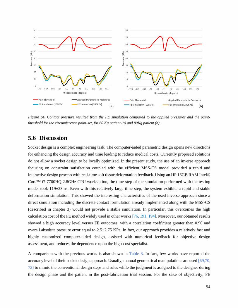
94
Figure 64. Contact pressure resulted from the FE simulation compared to the applied pressures and the paint-
threshold for the circumference point-set, for 60 Kg patient (a) and 80Kg patient (b).
5.6 Discussion
Socket design is a complex engineering task. The computer-aided parametric design opens new directions
for enhancing the design accuracy and time leading to reduce medical costs. Currently proposed solutions
do not allow a socket design to be locally optimized. In the present study, the use of an inverse approach
focusing on constraint satisfaction coupled with the efficient MSS-CS model provided a rapid and
interactive design process with real-time soft tissue deformation feedback. Using an HP 16GB RAM Intel®
Core™ i7-7700HQ 2.8GHz CPU workstation, the time-step of the simulation performed with the testing
model took 119±23ms. Even with this relatively large time-step, the system exhibits a rapid and stable
deformation simulation. This showed the interesting characteristics of the used inverse approach since a
direct simulation including the discrete contact formulation already implemented along with the MSS-CS
(described in chapter 3) would not provide a stable simulation. In particular, this overcomes the high
calculation cost of the FE method widely used in other works [76, 191, 194]. Moreover, our obtained results
showed a high accuracy level versus FE outcomes, with a correlation coefficient greater than 0.90 and
overall absolute pressure error equal to 2.5±2.75 KPa. In fact, our approach provides a relatively fast and
highly customized computer-aided design, assisted with numerical feedback for objective design
assessment, and reduces the dependence upon the high-cost specialist.
A comparison with the previous works is also shown in Table 8. In fact, few works have reported the
accuracy level of their socket design approach. Usually, manual geometrical manipulations are used [69,70,
72] to mimic the conventional design steps and rules while the judgment is assigned to the designer during
the design phase and the patient in the post-fabrication trial session. For the sake of objectivity, FE

95
simulation is usually performed to predict the pressure distribution on the stump surface during the
prosthetic use [71, 73]. It is well known that this complex FE simulation is very slow and impractical for
an interactive design system dedicated to clinical use. On the other hand, automated numerical approaches
[77-80] offer a foundation of an objective assessment criterion, but at the expense of design flexibility and
customization. In contrast, our approach provides an interactive, practical, rapid, highly customized, and
accurate design assisted with objective numerical real-time feedback.
Table 8. Comparison of the proposed approach with the available socket CAD systems
Soft tissue exhibits commonly a complex anisotropic, viscoelastic, inhomogeneous, nearly incompressible
behavior with large deformation. A large range of computational methods such as FE modeling methods
and their variations have been commonly used for developing soft-tissue deformation models [301]. Despite
Study Technique Design assessment Design
customization
Accuracy
(pressure
errors)
Ref.
The present study
Constraint-satisfaction technique based on an inverse approach
Numerical real-time feedback
Very high 2.5±2.75 KPa
Bonacini et al. 2007
3D-scan of the stump + CAD geometrical processing
FE simulation Equal to the
stump’s surface shape
N/A [71]
Hsu et al. 2010
Manual CAD manipulation
Personal judgement of the designer and post fabrication trial
Very high N/A [72]
Colombo et al. 2013
Manual CAD manipulation assisted by FE calculations
Personal judgement of the designer and FE simulation
Very high N/A [73]
Tzeng et al. 2015
Manual CAD manipulation
Personal judgement of the designer and post fabrication test
Very high N/A [70]
Colombo et al. 2016
Automatic modifications based on lifestyle and stump parameters
N/A Low N/A [77]
Nayak et al. 2016
Manual CAD manipulation
Personal judgement of the designer and post
fabrication test Very high N/A [69]
Steer et a. 2019
Statistical-Shape Model
Multiple solutions provided by the system. The final choice is made by the specialist.
Low < 4 KPa [79,80]
Li et al. 2019 Eigen vector algorithm method
Post-fabrication trial Low N/A [78]

96
a high accuracy level, the use of FE-related methods needs high computational cost and real-time feedback
can be also reached with model simplification or specific hardware implementation. Thus, real-time soft
tissue deformation remains a challenging issue in the biomechanical field. To provide an efficient approach,
a novel approach was proposed to estimate the soft tissue deformation using the Mass-Spring System
coupled with corrective springs (MSS-CS). The formulation simplicity and the low computational cost of
the MSS-based approach have been shown in many works from video games and computer graphics [302-
303] to surgical simulator domains [227, 233-237]. In particular, our proposed MSS-CS has been validated
with FE simulation outcomes with a commercial solver (i.e. Abaqus). This model was integrated into our
parametric workflow and provides real-time soft tissue deformation feedbacks with an average rendering
speed of 120 FPS and a calculation speed of 9 FPS. This is the first time that this approach has been applied
to the prosthetic domain. However, linear elasticity has been used to represent the behavior of soft tissues.
Further studies need to be investigated to add more realistic behavior of soft tissues into our MSS-CS model
to enhance the quantitative bio-feedbacks.
The interaction of the soft tissues with a medical device such as a socket in our study is extremely complex
to be described. This requires commonly multi-scale characterization and modeling for a better
understanding of tissue-device interface behavior [304-305]. Moreover, long-term analysis is required to
give a complete view of this complex interaction. The bone-implant interface has been largely studied [306-
307]. However, soft tissue interaction with the medical device remains a challenging issue. Especially in
the context of socket design, the relationship between mechanical loading and painful effects is still
misunderstood. To provide an efficient solution for this complex interaction, an inverse approach was
proposed in the present study. This approach is simplified but efficient to describe the stump-socket
interaction. To the best of our knowledge, this is the first use of the mass-spring system as well as the
inverse approach in the prosthetic design field. This allows developing the interactive design system, which
was not achieved in the case of direct FE calculations [76, 191, 194]. The inverse approach eliminates the
need for a contact formulation to predict the pressure distributions between the socket and the stump. It is
important to note that a discrete contact formulation implemented with the MSS-CS model takes around
48% of the calculation time. In addition, it requires decreasing the time-step size (or the calculation pseudo-
time) for the sake of stability which would slow down the simulation, as reported in chapter 3. Moreover,
the present work provides the first explicit and instant numerical feedback for an interactive prosthetic
socket design. Commonly, the prosthetic CAD consists of scanning the geometry of the residual limb and
then applying patient-specific modifications to the model, mimicking the artisanal conventional method
[90, 308-309]. This approach is followed by the currently used commercial prosthetic CAD systems where
the designed socket’s fit is still strictly correlated to the personal level of experience of the prosthetists as
well as the subjective feedback of the patient. Recently, automated socket design methods were proposed
and studied, either by using a predefined relationship between the geometrical operations and patient-
specific parameters [77], or by using previously fabricated sockets as dataset weighted based on the design

97
experience of the prosthetists [78], or even by parametrizing the design using Statistical-Shape Modeling
(SSM) [79]. However, pieces of the complete socket design are still missing. The first and second
approaches [77, 78] provide estimations of the magnitude of the geometrical modifications to be applied to
the stump model, without handling their sizes and locations. The SSM approach [79] provides an
approximated overall design concept based on the most influencing Principal Components (PCs) and
neglecting the information related to the low-influencing ones, and thus, it doesn’t provide the flexibility
to perform customized local geometrical operations for each specific patient. Moreover, these works are
strictly based on datasets reconstructed from manually fabricated sockets and that was not subject to an
objective assessment. The parametric tool implemented in our system overcomes these limitations by
allowing a highly customized design capacity including local geometrical operations. These operations are
parametrized in terms of their shapes, locations, sizes, and magnitudes. Furthermore, soft tissue
deformations are fed into the design process to adjust the design leading to an optimized solution satisfying
patient-specific geometrical and mechanical constraints.
In addition, the developed interactive design system with its user-friendly interface provides support to the
prosthetist’s evidence base. As shown in Figure 58, the manual manipulations to be applied are equivalent
to those performed while shaping the socket surface in the conventional fabrication method. What this
system adds to the clinical practice, in particular, is the parametric design tool for easy manipulations with
no need for CAD skills, along with visual feedback indicators in form of a radar chart as objective judgment
support. Moreover, the parametrization of the design opens the door for possible automatic optimization of
the socket. During the conventional socket test, the prosthetist looks for a pain-free prosthesis as a sign of
its comfortability. Our system uses the concept of the pain-threshold as a numerical translation of this
criterion for the sake of objectivity and independence from the subjective feedback of the patient. Instead
of the manual palpation to inspect the stump and estimate the socket shape modifications, the system
provides a tool dedicated to the reconstruction of the customized pain-threshold distribution. The
measurement of these thresholds is out of our scope but was the focus of many previous studies [126-130].
It is important to note that the paint-threshold measuring is still not a simple task to carry out, and relies on
the subjective feedback of the patient since the pain is a subjective personal experience unable yet to be
measured. Furthermore, the visual feedback indicators simplify for the prosthetist the engineering concepts,
so he can reach a surface pressure pattern that is equivalent to the contact pressure with the well-fit socket,
in other terms, to reach a deformed surface that is equivalent to the shape of the socket he’s looking for.
The main limitation of this study deals with the fact that only static standing up with normal pressure effect
was considered as loading condition. It is well-known that stump-socket interaction is highly dynamic.
Thus, the dynamic mechanism should be further integrated into the proposed inverse approach taking into
consideration the shear behavior. Moreover, the accuracy of the proposed method is highly dependent on
the quality of the generated mesh of the stump model. Highly irregular elements lead to undesired

98
deformations. In particular, the MSS-CS model is based on the hexahedral mesh whose generation is still
not a simple task. Further future works related to the enhancement of the MSS-CS model and meshing
process may be carried out.
Another limitation of the present study relates to the use of a dataset from a normal subject to fabricate the
stump model. Thus, the application of the proposed process should be applied to real patients with a residual
stump structure. For this purpose, the visual sensor fusion solution developed (described in the previous
chapter) could be used to acquire the 3D geometries of the stump, and the generated model will be integrated
into our present process. Finally, our interactive design process requires manual manipulations with the
clinician’s expertise to adjust the design based on soft tissue deformation feedbacks. Thus, this design
approach may be later automated and optimized using an automatic optimization algorithm.

99
General Discussions
In this chapter, the thesis objective is recalled, our achievements are summarized and generally discussed,
and our scientific and technical contributions along with our system limitations are highlighted.
6.1 Thesis objective
This project aims to study a way to optimize the design process of the lower limb prosthetic socket, in terms
of production time, cost, and design reliability. Since the prosthetic socket is a tailor-made product designed
to fit with the residual limb of the amputee having unique shape and characteristics, establishing numerical
standards for the design and realization of the prosthetic socket is still not a simple task. The current socket
design practice is still manual and based on the personal know-how of a specialist, its subjective judgment
based on his experience, and the feedback of the patient during the post-fabrication trial sessions. Even the
provided CAD systems still follow this manual approach. Usually, a trial-rectification iterative process is
needed until reaching the well-fit socket that acquires the amputee’s satisfaction. Thus, this is a long-time-
consuming process, high-cost, and based on subjective assessment criteria that negatively impact the design
reliability. Establishing an alternative optimized socket design and fabrication process is needed to enhance
prosthetic production.
It is assumed that a fully numerical alternative solution is mainly based on the digital model of the patient’s
stump including all its unique features. Therefore, a typical workflow of such a process consists, of four
main steps (Figure 2): scan of the residuum, generating the residual limb model, numerical computer-aided
design of the socket, computer-aided manufacturing. This thesis focuses on the three main steps related to
the design phase, and the objective is to propose and study a complete prosthetic design system from limb
scanning and system modeling to the digital socket shaping, providing a fully numerical solution for the
socket design, to objectify the socket analysis, reduce the process time and cost, and eliminate the
dependence upon skilled orthopedists.
6.2 The achieved system
During the three years of work, we eventually realized a fully numerical prosthetic socket computer-aided
design process whose input is the patient’s biological limb, and output is the virtual model of the
corresponding socket (Figure 65).

100
Figure 65. the diagram of the achieved system
After receiving the amputee, the process starts by 3D scanning the residuum’s geometry using the Kinect-
fusion scanning platform. Microsoft Kinect v2 sensors are used for their low-cost and scanning potential,
and four sensors were combined for a rapid scan. A 3D geometrical model of the stump is then given in
STL (stereolithography) format. The model is meshed following a hexahedral configuration and the related
Mass-Spring model is generated. The Mass-Spring System (MSS) is proposed in this project as an
alternative to the widely used Finite Element Method (FEM) to model the deformations of the stump’s soft
tissues, thanks to its simplicity and relatively low computational cost. In fact, in the context of an interactive
design process with real-time quantitative feedback provided during the interactive shaping of the socket,
or even in the case of an automatic design optimization process, a rapid calculation becomes crucial. A new
configuration of the MSS is proposed to add to the model the volume conversation property of the soft
tissues, by introducing non-linear diagonal Corrective Springs (CS) whose stiffness is variable in function
of the volume change. After the modeling step, the MSS-CS model of the stump is imported by a socket
parametric design platform, where real-time numerical feedback is given to assist the designer and guide
the designing process. The feedback comes from constraints postulated as a numerical definition of the
design of the well-fit socket and is displayed in a radar-chart. The real-time calculations were possible
thanks to the simplicity of the MSS-CS model along with the use of the inverse calculation to estimate the
stump-socket interaction stresses.

101
A good precision level is required in the prosthetic design application since it is known that the fit-quality
of the socket is highly sensitive to small changes in the socket dimensions. The accuracy of each step of the
system’s workflow has been measured and compared to previous similar works. The fusion scheme of the
Kinect v2 sensors with the applied error reduction techniques showed a remarkable reduction level of 3D
geometrical reconstruction errors compared to state-of-the-art scanning techniques. The absolute error
values of the 3D geometrical reconstruction of a stump-like cylindrical object are between 1.2mm and
1.8mm which are 0.8% to 1.3% relative to the scanned object diameter, versus 2.75mm average error using
the ultrasound scan [191], 1.4% to 4% (and may sometimes reach 8%) using the image processing technique
[99], and 1.4% to 2% using a portable scanner [98]. At the modeling level, it is the first time that the MSS
is applied in the prosthetic field, therefore it was not possible to compare our results with peer research in
the literature. The outcomes of the MSS-CS calculations were compared to those coming from valid FE
software (Abaqus). These two data outputs showed a correlation coefficient equal to 0.77 for a stump-socket
interaction during a donning process, and 0.90 to 0.95 for the final output of the system (the socket design).
The higher errors given by the interaction simulation may be due to the different contact formulations used
in Abaqus and our MSS-CS simulator, and a high correspondence is shown in the design step where the
inverse calculation approach is applied (without direct contact calculation) which reveals a good precision
level in the deformation calculation of the soft tissues using the MSS-CS model.
The process is fully numerical. It is based on a numerical model of the residual limb, captured by the
scanning step and automatically modeled by the second step. Still, some parameters related to the model
are to be provided manually such as the elastic modulus of the soft tissues, and the pain-threshold on the
surface of the stump. Actually, these two parameters are the numerical translation of the palpation
performed by the prosthetist in the conventional method to inspect the stiffness of the soft tissues and
estimate the pressure-sensitivity at the key-points of the residuum. Furthermore, manual manipulations are
still required to be performed in the socket design step mimicking the shaping steps in the conventional
method. However, these manipulations are parametrized for easier application in the current system, and
for potential future automation of the process. On the other hand, the numerical definition of the well-fit
socket, given in equations 42, 44, 45, and 47, provides a numerical approach for the design evaluation,
which is instantly given to the designer during the designing phase as an objective assistant. This original
point, which is not reported so far in the literature, is a numerical alternative to the subjective interpretation
of the patient’s feedback by the personal experience of the prosthetist.
Our socket parametric design method assisted with real-time feedback can be framed as a formal
engineering design optimization problem. In this case, the parameters of the applied parametric pressures
function as design parameters across a multi-dimensional input space, and the resultant contact pressure
field is formulated as the objective function (also called cost function). Since the discomfort is usually
associated with the contact pressures, the objective is to minimize the formulated cost function to reduce

102
the pain and thus increase comfort. It is also managed by the postulated constraints that ensure the stability
as well as the correspondence of the input parameters with the mechanical formulations. Whereas our
system consists of manual tuning of the input design parameters following a trial-error approach to find a
possible solution to this optimization problem, it is also possible, as future work, to elaborate an
optimization solver looking for the optimal solution.
The system does not provide an optimization just for the socket design not also for the production process
itself. The target here is to reduce the cost and time of the design and fabrication process, therefore, the
objective/cost function is to be formulated as a function of these two parameters. First, the capital cost of
the system has been reduced thanks to the cheap Kinect sensors that we’ve used. Besides, it consists of a
CAD system that does not require highly skilled labor. Second, this process effectively reduces the
production time. Whereas a socket consumes several days to be shaped in the current practice [46], it needs
no more than a half-hour to be designed by our system, thanks to the postulated numerical criterion to assess
the socket design that is supposed to eliminate the need for repetitive trial/rectification sessions. The Kinect-
fusion scheme allows relatively rapid scanning of the limb that takes almost 25 seconds (Figure 50), the
modeling step takes around 2 minutes, and the whole parametric design process (Figure 58) that produces
the final socket model took no more than 15 minutes. In addition, this is a low capital system requiring one
workstation and the four-Kinects scanning platform, knowing that Microsoft Kinect cameras are relatively
cheap devices brought to the market at a price equal to a couple of hundreds of dollars for each one. It is
important to note here that most prosthetists don’t rely on a numeric scan of the residual limb either because
of the high-cost as in the case of the medical imaging techniques and expensive optical scanners or because
of the low accuracy level, especially for the commercial low-cost portable scanners. Considering the
previously discussed accuracy level of our scanning platform, our system represents a good Quality/Price
solution hoping that it will be more attractive to be used in the prosthetic field.
Every step of the whole workflow has been implemented with an interactive graphical user-friendly
interface (GUI) including widgets for 3D visualization and manipulation along with all necessary functions,
to enhance the efficiency and ease of use for the underlying algorithms and numerical methods described
in this thesis. The scanning GUI (Figure 43) accommodates graphical interaction elements related to system
calibration, scanning and point-cloud generation, filtering, surface reconstruction, and model export to the
well-known STL format. The GUI of the MSS-CS simulator and parametric socket design platform (Figure
55) is realized with clinical-friendly widgets and functions that represent every clinically performed step in
the conventional socket shaping process.
The design of this GUI has followed the suggestions and feedback of the specialists in ELIMED orthopedic
center, Beirut, Lebanon (http://www.elimedcenter.com/) who satisfactorily evaluated the final system. The
concept used in the clinically applied commercial CAD systems is maintained, but with an additional
parametrization feature which enhances the ease of use and reduces the need for CAD skills. The numerical

103
design assistant represented by the numerical feedback given as a radar chart (Figure 55d) is also an original
point that is not provided in the currently used systems, and it also received a positive evaluation from the
specialists. However, this was limited for being a “concept evaluation” of the specialists’ impressions of
this prospective system, and no clinical experimental evaluation is yet performed.
6.3 Main contributions
6.3.1 MSS-CS model for fast soft-tissues deformation
MSS-CS (Mass-Spring System + Corrective Springs) is a model that was proposed in this study to estimate
the deformations of the stump’s soft tissues. The choice of the mass-spring-based system is motivated by
its simplicity and low computational cost allowing to perform fast dynamic simulations, unlike the very
expensive and widely used FE method. This system attracted the interest of many researchers to simulate
the soft tissue behavior in various medical fields, however, it is still not introduced in the prosthetic
application. MSS-CS provides a new configuration for the mass-spring system to simulate the non-
compressibility of the soft tissues, by introducing non-linear volume correction springs whose stiffnesses
are variable in function of the volume variation.
6.3.2 Error compensation strategy for the Kinect v2 sensor
The Kinect v2 raw outputs (x, y, and depth) are subject to some errors. Beside the literature, our observation
shows that the errors are somehow correlated to the output values, which opens the door for possible errors’
modeling. For this purpose, a machine learning system based on the linear regression method was
implemented to predict the errors for each pixel of the output frame of the sensor. The predicted errors are
then used in an error compensation algorithm. Using this approach, the errors have been reduced up to 50%
for every single sensor.
6.3.3 OpenMKS 3D-scanning platform
OpenMKS (Open Multi-Kinect Scan) is an open-source C++ code that we’ve developed as a tool for rapid
and accurate 3D-scanning and shared with the scientific community. The underlying scanning method is
based on the fusion of multiple low-cost RBG-Depth Microsoft Kinect v2 sensors. The implementation
includes a technical solution for the multi-sensor-fusion to one workstation and the aforesaid error
compensation strategy along with an iterative multi-set registration that increased the scan accuracy and
reduced the scanning errors up to 40%. OpenMKS provides a relatively good scanning precision level, and
a rapid scan that takes around 25 seconds, whereas it is reported to take several minutes in other works.

104
6.3.4 Constraint satisfaction approach for a numerical socket design with
real-time feedback
Based on the inverse calculation of the stump-socket interaction, arithmetic constraints have been
postulated to define the shape of the well-fit socket. The expected optimal solution is the one that satisfies
the given constraints. These constraints are the basis of the numerical feedback given to guide the designer.
Real-time feedback was possible thanks to the cheap contact-free inverse approach and the fast MSS-CS
deformations’ calculations. The research in the literature suggests that this is the first numerical design
method with a numerical definition of the socket shape and real-time numerical feedback so far.
6.4 Limitations
Our system still exhibits limitations, part of which was already discussed in previous chapters, and further
developments are needed to fill the gaps.
At the scanning level, only the outer surface of the stump is captured and digitized, and no information
about the bony structures and the biomechanical parameters of the soft tissues is directly collected from the
limb. It is important to note that this missing information is necessary to complete the MSS-CS model. In
the tests executed in this thesis, the bones were acquired from the CT dataset and manually placed inside
the model, and the used values of the biomechanical properties of the soft tissues are estimated based on
the literature reported values. In addition, two types of calibration are needed for our scanning platform:
the individual calibration of each sensor to identify the parameters of the relevant error compensation
system, and the overall system calibration for accurate multi-set registration. While the former calibration
type can be performed once during the manufacturing phase, the latter one is necessary before each use
considering the potential risk of system displacement, sensor tilting or movement... etc., which adds up the
time and efforts of a technical task to the clinical practice. The orthopedic technicians of ELIMED center
reported dissatisfaction from the fact that the scanning platform is not mobilizable and has large dimensions
(1.5m × 1.5m). Many of the center’s customers are unable to leave their homes, and the orthopedist, usually,
visits them to inspect the limb and scan it when necessary. The commercial portable calibration-free
scanners are preferable in these cases, despite their disadvantage related to the slow scanning process that
increases the risk of errors related to the involuntary muscles’ contraction or limb movement.
At the modeling level, the soft tissues are simplified as a linear viscoelastic object, knowing that they are
inhomogeneous viscoelastic material with complex biomechanical behavior. This simplification is
motivated by the assumption that the stump-socket interaction does not present large deformations that
would reach the non-linear zone. On the other hand, both linear and hyper-elastic models were tested in
previous work [191], and results show similar pressure distribution for both cases but a considerably higher
simulation speed in the case of the linear model. The shear behavior of the MSS-CS model was not

105
investigated. It is important to note that this is still a main issue of the Mass-Spring -based models for the
spring, as a fundamental element in mechanics, does not have a shear property. Besides, the human limb is
known for its very high level of anatomical complexity consisting of muscles, fat, dermic layer, blood
vessels, nerves… etc. Usually, the whole volume of the stump (excluding the bony structure) is simplified
as a homogenous elastic object [74, 180, 181, 194], and a layer representing the liner is sometimes
differentiated and added to the model [186]. The current proposed model follows the former approach,
though it has the potential to follow the latter one.
The MSS-CS model is based on a hexahedral meshing configuration. One of the main issues of this point
is the fact that hexahedral meshing is still not a simple task to be performed, especially for 3D objects with
a non-standard geometric shape. For the moment, this task is executed using the open-source meshing tool
IA-FEmesh [246] and not yet introduced as an underlying function in our system after the scanning step.
One of the very important parameters involved in the designing phase is the pain-threshold distribution. It
is known that this is a unique feature that varies from one patient to another depending on the characteristics
of the residual limb, along with local tissue sensitivities associated with neuromata and soft tissue injuries
which are usually identified in limb assessment by the prosthetist. Pain is a subjective experiment that is
still not able to be directly measured. Usually, pressure sensitivity is measured over various regions of the
stump by mechanical indentation looking for the minimum pressure from which the patient reports feeling
pain [127-131]. This process still relies on the subjective feedback of the patient that can’t be objectively
validated. Anyway, our developed system is still missing this step for it requires an indentation measuring
device, and estimated values found in the literature are currently assigned to the model.
The proposed socket design approach is based on the inverse calculation of the stump-socket interaction
where the well-fit socket is defined by certain postulated constraints that rule the pressure distribution to be
applied to the stump surface. These constraints are derived from a simplified analytical study of the static
stump-socket interaction, but this approach was not clinically validated. The complex mechanical behavior
of the system (during the gait cycle for instance) is not involved in the calculation. It is important to note
that, in the current conventional clinical practice, both static and dynamic tests are performed to assess the
fabricated socket. Therefore, the proposed approach yet does not fulfill all the clinical expectations,
especially regarding the comfortability of the socket during the dynamic usage of the prosthetic device.
Finally, the system has been validated numerically but was not brought to the clinical environment for
experimental validation, which was unfortunately prevented due to the COVID-19 situation. Consequently,
each step of the system has been studied and evaluated separately, whereas no test for the complete
workflow has been performed for global evaluation. It is known that user satisfaction with the socket is
ultimately a subjective measure that depends on a range of human factors such as comfort, pain thresholds,
and proprioception arising from a firm, functional prosthesis-skeletal coupling. This means that the
predictions of pressures and soft tissue strain are not necessarily directly related to comfort [310]. Thus,

106
actual experimental tests are necessary to validate the postulated numerical definition of a comfortable
socket and report the satisfaction level of the patients. Besides, the current system accommodates some
parameters to be tuned. For instance, the constants of the MSS-CS model were manually tuned to reach FE-
like results, but yet not experimentally validated as an actual reflection of the behavior of the soft tissue.

107
Conclusions & Perspectives
7.1 Summary of the thesis
The initial objective of this thesis was to study and develop a numerical-based alternative process for the
design of the lower-limb prosthetic socket, which shall lead to cost reduction and design optimization. The
socket is the most critical part of the device and consumes the most time and effort of the overall design
and fabrication process of the prosthesis. The review of the state-of-the-art in the prosthetic field shows that
this industry still relies on an artisanal and subjective process where the fit-quality of the final socket is
strictly correlated with the orthopedic technicians’ skills. Even the currently existing computer-aided design
(CAD) systems are based on the same manual approach. That’s why the prosthetic industry needs an
alternative approach that optimizes prosthetic production.
During the three years of this thesis, the initial objective has been achieved by proposing and studying an
innovative CAD-based socket design workflow. The proposed solution is totally based on the virtual model
of the patient’s residual limb which has to be generated for each patient. Thus, the primary three steps of
this process are elucidated as the 3D scan of the residuum, the generation of the related virtual model, and
finally the CAD of the socket. Each of these steps was given specific focus and studied in a way to overcome
the limitations existing in the current related techniques. As for the 3D scanning, we proposed a fusion
scheme of four Kinect v2 sensors along with error reduction techniques. The scanned model is then meshed
and a Mass-Spring based model of the residual limb soft tissues is generated. To our knowledge, this is the
first time that the Mass-Spring System (MSS) is applied in the prosthetic field, although it is popular in
many other medical-related applications. A new configuration involving Corrective Springs (CS) is
proposed to add volume conversation property to the model. This approach offers a fast stress-strain related
calculation of the soft tissues, unlike the widely used Finite Element (FE) method. This fast calculation
plays a significant role in the socket CAD method that we proposed, where an inverse calculation of the
stump-socket interaction is used to provide real-time numerical feedback during the designing phase.
Parametric CAD tools have been implemented in a user-friendly interface.
The system has been validated numerically. The 3D scan exhibits a good level of accuracy compared to
previous peer works, while the results of the modeling approach and the design method show good
correspondence to the Finite Element (FE) outcomes. The achieved system has received a satisfactorily
concept evaluation from experienced prosthetists, and it is to be brought to the clinical environment for
experimental validation.

108
7.2 General perspectives
Beside the further work needed to enhance the system, fill the gaps, and overcome its limitations, this
project opens the door for both short- and long-term perspectives.
Further studies are needed to enhance the MSS-CS model, in order to reflect the real complex viscoelastic
behavior of the stump soft-tissues and speed-up the calculation. Experimental validation shall be carried
out to compare the MSS-CS outcome with real stresses’ and strains’ measurements.
In order to complete the modeling step, internal bony structures need to be also reconstructed. Usually,
MRI and CT scans are used to collect the internal geometries [59, 70, 73, 97-101], and this may be a possible
solution whenever medical imaging has been already performed in the clinic. In many cases, however,
medical images are not available, knowing that a prosthetic device may be ordered anywhen during the life-
time. MRI and CT are expensive techniques and not favorable to the low-cost production process. A
potential candidate for this purpose can be the statistical shape modeling method or any other machine-
learning-based method that can study the relationship between the stump surface morphology and the inner
bones’ geometry toward an automatic generation of the latter one. This step can be implemented as an
underlying function in the system along with an automated meshing algorithm to facilitate the use of the
system in the clinical context.
In the context of short-term perspectives, the dynamic interaction between the stump and the socket will be
studied and introduced in the system. There exist various platforms designed to study and analyze the
human gait cycle along with other dynamic movements, such as OpenSim [311]. This is a suitable tool for
studying the dynamic behavior of the stump-socket system, which can be brought to our design environment
by developing an interface that connects OpenSim simulations with our MSS-CS simulator. The system
will allow, thus, a pre-fabrication prediction of the socket comfortability during the dynamic, replacing the
currently practiced post-fabrication dynamic trial sessions.
The ultimate long-term target is to automate the prosthetic production process. While this is still unfeasible
due to the lack of numerical definition of the optimal design, the approach presented in this thesis
transformed the socket design problem into a constraint’s satisfaction problem and provides a
parametrization of the socket shape. This opens the door for future investigation of an optimization
algorithm whose input is the stump model, and output is the values of the shape parameters that should
satisfy the given constraints.
The results of virtual tests and simulations show that the proposed solution is promising for improving the
current prosthetic production and overcoming its limitations such as subjectivity, high-time consummation,
and dependence on high-cost expertise. In addition, a positive concept evaluation has been received from
qualified prosthetists. However, future clinical experiments are needed to be done to validate the system
outcomes and report the satisfaction level of both patients and prosthetic specialists. For this purpose,

109
testing prototypes of the designed socket shall be fabricated, and the final socket is to be produced. A
Computer-Aided Manufacturing (CAM) technique, which was not within the scope of this thesis, shall be
studied to complete the prosthetic design and fabrication system.
This thesis created the foundation for a prosthetic CAD application but also contributed to other fields. For
instance, OpenMKS provides a rapid and low-cost solution whenever a 3D-scan is needed. The MSS-CS
system is intended to model the biomechanical behavior of the soft tissues and can be applied in other
medical or biomechanical fields where the fast calculation of soft tissue deformations is required, as well
as in computer vision applications. The inverse interaction calculation approach can be a solution wherever
the identification of a contract surface shape is challenged by the complexity and the high cost of the direct
contact calculation.
The system that we started to develop needs a lot of refinements and developments and its progress does
not stop at the end of this thesis. As this project ends with new questions, a tremendous amount of work
and scientific studies is ahead of us to enhance our findings and upgrade our achieved system. That’s it, the
path never ends, the more we advance, the more the road opens to our eyes. And as we progress, we hope
that each step we make adds new knowledge to the scientific community, and contributes to the
improvement of human life.

110
Publications
National Conference
• A. Ballit, I. Mougharbel, H. Ghaziri, T-T. Dao, “Fast Soft Tissue Deformation toward a Computer-Aided
Design System for Lower Limb Prostheses”, JETSAN 2019, Paris, France.
Journal Articles
• A. Ballit, I. Mougharbel, H. Ghaziri, and T.T Dao, “Fast Soft Tissue Deformation and Stump-Socket
Interaction toward a Computer-Aided Design System for Lower Limb Prostheses,” Innovation and Research
in BioMedical Engineering (IRBM), In Press, 2020
• A. Ballit, I. Mougharbel, H. Ghaziri and T. Dao, "Visual Sensor Fusion with Error Compensation Strategy
toward a Rapid and Low-cost 3D Scanning System for the Lower Residual Limb," in IEEE Sensors Journal,
doi: 10.1109/JSEN.2020.3011172.
• A. Ballit, I. Mougharbel, H. Ghaziri, and T.T Dao. “Computer-aided Parametric Prosthetic Socket Design
based on Real-Time Soft Tissue Deformation and an Inverse Approach”, The Visual Computer, International
Journal of Computer Graphics, 2020. (Under Review)

111
References [1] Ziegler‐Graham K, MacKenzie EJ, Ephraim PL, Travison TG, Brookmeyer R. Estimating the
Prevalence of Limb Loss in the United States: 2005 to 2050. Archives of Physical Medicine and
Rehabilitation2008;89(3):422‐9.
[2] Owings M, Kozak LJ, National Center for Health S. Ambulatory and Inpatient Procedures in the
United States, 1996. Hyattsville, Md.: U.S. Dept. of Health and Human Services, Centers for Disease
Control and Prevention, National Center for Health Statistics; 1998.
[3] Abbas ZG. The global burden of diabetic foot. In: Pendsey S, editor. Contemporary Management of
the Diabetic Foot. 1st ed. New Delhi: Jaypee Brothers Medical Publishers (P) Ltd.; 2013
[4] Pasquina PF, Miller M, Carvalho AJ, Corcoran M, Vandersea J, Johnson E, Chen YT. Special
considerations for multiple limb amputation. Current physical medicine and rehabilitation reports.
2014 Dec 1;2(4):273-89
[5] Horgan O, MacLachlan M. Psychosocial adjustment to lower-limb amputation: A review. Disabil
Rehabil. 2004;26:837–50.
[6] Solgajová A, Sollár T, Vörösová G. Gender, age and proactive coping as predictors of coping in
patients with limb amputation. Kontakt. 2015;17:e67–72.
[7] Pell JP, Donnan PT, Fowkes FG, Ruckley CV. Quality of life following lower limb amputation for
peripheral arterial disease. Eur J Vasc Surg. 1993;7:448–51.
[8] Parkes CM. Components of the reaction to loss of a lamb, spouse or home. J Psychosom Res.
1972;16:343–9
[9] Kingdon D, Pearce T. In: Psychological assessment and management of amputee. In: Rehabilitation
of Management of the Amputees. Banarjee S, editor. Baltimore, MD: Williams Wilkins; 1982. pp.
350–71. [Google Scholar]
[10] Block WE, Ventur PA. A study of the psychoanalytic concept of castration anxiety in symbolically
castrated amputees. Psychiatr Q. 1963;37:518–26. [PubMed] [Google Scholar]
[11] Goldberg RT. New trends in the rehabilitation of lower extremity amputees. Rehabil Lit. 1984;45:2–
11.
[12] Parkes CM.. Psychosocial transitions: comparison between reactions to loss of a limb and loss of a
spouse. Br J Psychiatry. 1975;127:204–210.
[13] Kubler-Ross E. On Death and Dying. New York, NY: Simon & Schuster; 1969.

112
[14] McGimpsey, G., Bradford, T., 2010. Limb Prosthetics Services and Devices. Bioengineering Institute
Center for Neuroprosthetics, Worcester Polytechnic Institution, Worcester, MA
[15] Mackenzie EJ, Jones AS, Bosse MJ et al. Health-care costs associated with amputation or
reconstruction of a limb-threatening injury. J. Bone Joint Surg. Am. 89(8), 1685–1692 (2007)
[16] Blough DK, Hubbard S, Mcfarland LV, Smith DG, Gambel JM, Reiber GE. Prosthetic cost projections
for servicemembers with major limb loss from Vietnam and OIF/OEF. J. Rehabil. Res. Dev. 47(4),
387–402 (2010).
[17] Alemayehu B, Warner KE. The lifetime distribution of health care costs. Health Serv. Res. 39(3), 627–
642 (2004).
[18] L. Lorenzelli, et al.” Socketmaster: Integrated Sensors System for the Optimised Design of Prosthetic
Socket for above Knee Amputees”, Published in: CAS (NGCAS), 2017 New Generation of, 6-9 Sept.
2017, pp. 233-236.
[19] N. Herbert, D. Simpson, W. D. Spence, W. Ion, “A Preliminary Investigation into the Development of
3-D Printing of Prosthetic Sockets”, JRRD, Vol.42, N.2, March/April 2005, p.141-146
[20] Syme, J.: Amputation at the ankle joint. Med. Sci. (Lond./Edinb.) 3 (1843), 93–96.
[21] Center for International Rehabilitation Research Information and Exchange, Partial Foot Amputation:
Aetiology, Incidence, Complications, Prosthetic Intervention and a Characterisation of Gait. Retrieved
January 05, 2017, from http://cirrie.buffalo.edu/encyclopedia/en/article/154/
[22] Owings MF, Kozak LJ. Ambulatory and inpatient procedures in the United States, 1996. Vital Health
Stat 13 1998;13(139):1-119.
[23] 50. Spittler, AW, Brennan, JJ, Payne, JW. Syme amputation performed in two stages. J Bone Joint
Surg Am. 1954;36(1):37-42.
[24] Waters, RL, Perry, J, Antonelli, D, Hislop, H. Energy cost of walking of amputees: the influence of
level of amputation. J Bone Joint Surg Am. 1976;58(1):42-46.
[25] Gaine, WJ, McCreath, SW. Syme’s amputation revisited: a review of 46 cases. J Bone Joint Surg Br.
1996;78(3):461-467.
[26] Smith, DG, Sangeorzan, BJ, Hansen, ST, Burgess, EM. Achilles tendon tenodesis to prevent heel pad
migration in the Syme’s amputation. Foot Ankle Int. 1994;15(1):14-17.
[27] Smith, D. G. (2014, February). The Knee Disarticulation:It's Better When It's Better and It's Not When
It's Not.

113
[28] Higgins TF, Klatt JB, Beals TC. Lower Extremity Assessment Project (LEAP)--the best available
evidence on limb-threatening lower extremity trauma. Orthop. Clin. North Am. 2010 Apr;41(2):233-
9.
[29] American Physical Therapy Association. (2015, June 16). Above-Knee Amputation. Retrieved
January 06, 2017, from:
http://www.moveforwardpt.com/symptomsconditionsdetail.aspx?cid=7e9549ef-0bff4b50-88f1-
8a8bf4f1e49615
[30] Pedersen HE. The problem of the geriatric amputee. Artif Limbs. 1968 Autumn;12(2):Suppl:1-3
[31] Köhler P, Lindh L, Björklind A. Bacteria on stumps of amputees and the effect of antiseptics. Prosthet
Orthot Int. 1989;13(3):149–51.
[32] Hachisuka K, Nakamura T, Ohmine S, Shitama H, Shinkoda K. Hygiene problems of residual limb
and silicone liners in transtibial amputees wearing the total surface bearing socket. Arch Phys Med
Rehabil. 2001;82(9):1286–90. [PMID:11552206].
[33] de Laat FA, van der Pluijm MJ, van Kuijk AA, Geertzen JH, Roorda LD. Cosmetic effect of knee joint
in a knee disarticulation prosthesis. Journal of Rehabilitation Research and Development. 2014
;51(10):1545-1554. DOI: 10.1682/jrrd.2014.03.0068.
[34] Apffelstaedt JP, Driscoll DL, Karakousis CP. Partial and complete internal hemipelvectomy:
complications and long-term follow-up. J Am Coll Surg. 1995;181:43-48
[35] Shmookler, B., Bickels, J., Jelinek, J., Sugarbaker, P., & Malawer, M. M. (2001). Bone and Soft-tissue
Sarcomas: Epidemiology, Radiology, Pathology and Fundamentals of Surgical Treatment. Retrieved
January 06, 2017
[36] Agarwal M, Puri A, Anchan C, Shah M, Jambhekar N (2007). "Rotationplasty for bone tumors: is
there still a role?". Clin. Orthop. Relat. Res. 459: 76–81. doi:10.1097/BLO.0b013e31805470f0
[37] Nerlich AG, Zinc A, Szeimies U, Hagedorn H: Ancient Egyptian prosthesis of the big toe. Lancet 356:
2176–2179, 2000
[38] Burkard Jr., G.; Rizzo, J.-R.; Heckman, J.; Cohen, J. Chapter 15 Prosthetics. In Rehab Clinical
Pocket Guide: Rehabilitation Medicine; Sackheim, K.A. Ed. Springer: New York, 2013; pp 529-
555.
[39] Sanders, J.E. (2005). Stump-Socket Interface Condition. In D. Bader, C. Bouten, D. Colin & C.
Oomens (eds.), Pressure ulcer research current and feature prespectives (pp. 129). Berlin, Germany:
Springer, 129–148.

114
[40] Fergason J and Smith D.G (1999) Socket Considerations for the Patient With a Trans-Tibial
Amputation Clinical Orthopaedics and Related Research 361 pages76-84
[41] Paternò L, Ibrahimi M, Gruppioni E, Menciassi A, Ricotti L. Sockets for limb prostheses: a review of
existing technologies and open challenges. IEEE Transactions on Biomedical Engineering. 2018 Jan
23;65(9):1996-2010.
[42] Hagberg K, Branemark R. Consequences of non-vascular transfemoral amputation: a survey of quality
of life, prosthetic use and problems. Prosthet Orthot Int 2001;25:186–194
[43] 2. Meulenbelt HE, Geertzen JH, Jonkman MF, Dijkstra PU. Determinants of skin problems of the
stump in lower-limb amputees. Arch Phys Med Rehabil 2009;90:74–8
[44] Safari M, Tafti N, Rezasoltani P. Effect of 'bad' and 'good' socket fit on functional capability of below
knee amputees. Iran J War Public Health. 2013; 5 (4) :51-60
[45] S. Turner, A. H. McGregor, “Perceived impact of socket fit on major lower limb prosthetic
rehabilitation: a clinician and amputee perspective”, Archives of Rehabilitation Research and Clinical
Translation, Available online 21 May 2020, 100059.
[46] Pezzin LE, Dillingham TR, MacKenzie EJ et al (2004) Use and satisfaction with prosthetic limb
devices and related services. Arch Phys Med Rehabil 85:723–729.
https://doi.org/10.1016/j.apmr.2003.06.002
[47] J. A. De Lisa et al., Physical Medicine and Rehabilitation: Principles and Practice. Hagerstown, MD:
Lippincott Williams & Wilkins, 2005.
[48] J. T. Highsmith and M. J. Highsmith, “Common skin pathology in LE prosthesis users: the nature of
state-of-the-art skin-prosthesis interface puts amputees who use prostheses at increased risk for these
common dermatologic conditions,” JAAPA, vol. 20, no. 11, pp. 33–38, Nov. 2007.
[49] Muller M, Staats T.B, Leach M and Fothergill I , Total Surface Bearing Trans-Tibial Socket Design
Impression Techniques
[50] Yiğiter K, Şener G and Bayar K (2002) Comparison of the Effects of Patellar Tendon Bearing and
Total Surface Bearing Sockets on Prosthetic Fitting and Rehabilitation Prosthetics and Orthotics
International 26 206-212
[51] Moo E.K, Osman N.A.A, Pingguan-Murphy B, Wan Abas W.A.B, Spence W.D and Solomonidis S.E
(2009) Interface Pressure Profile Analysis for Patella Tendon Bearing Socket and Hydrostatic Socket
Acta of Bioengineering and Biomechanics 11(4) 37 – 43

115
[52] Hachisuka K, Dozono K, Ogata H, Ohmine S, Shitama H, Shinkoda K (1998) Total Surface Bearing
Below – Knee Prosthesis: Advantages, Disadvantages and Clinical Implications Archives of Physical
Medicine and Rehabilitation 79 783-789
[53] S. Fatone and R. Caldwell, “Northwestern University Flexible Subischial Vacuum Socket for persons
with transfemoral amputation: Part 2 Description and Preliminary evaluation,” Prosthet. Orthot. Int,
vol. 41, no. 3, pp. 246–250, Jun. 2017.
[54] R. D. Alley et al., “Prosthetic sockets stabilized by alternating areas of tissue compression and release,”
JRRD, vol. 48, no. 6, pp. 679– 96, Jun. 2011
[55] J. T. Kahle and M. J. Highsmith, “Transfemoral interfaces with vacuum assisted suspension
comparison of gait, balance, and subjective analysis: Ischial containment versus brimless,” Gait
Posture, vol. 40, no. 2, pp. 315–320, Jun. 2014.
[56] D. Kijkusol, " Simplified, low cost below-knee prosthesis". Siriraj Hospital, Mahidol University,
Bangkok, Thailand. Prosthetics and Orthotics International, 1986, 10, 96-98. DOI:
10.3109/03093648609164507
[57] P. V. S. Lee, N. Lythgo, S. Laing, J. Lavranos, N. H. Thanh, “Pressure Casting Technique for
Transtibial Prosthetic Socket Fit in Developing Countries”, JRRD, vol. 51, no. 1, pp. 101-110, 2014.
DOI: 10.1682/JRRD.2012.10.0191
[58] J. Andrysek. "Lower-limb prosthetic technologies in the developing world: A review of literature from
1994–2010". Prosthetics and Orthotics International December 2010; 34(4): 378–398
[59] A. J. Petron. "Prosthetic Socket Design: From a Multi-Indenter Device for in vivo Biomechanical
Tissue Measurement to a Quasi-passive Transtibial Socket Interface". MASSACHUSETTS
INSTITUTE OF TECHNOLOGY. February 2016.
[60] David M. Sengeh, Kevin M. Moerman, Arthur Petron, Hugh Herr. "Multi-Material 3-D Viscoelastic
Model of a Transtibial Residuum from In-vivo Indentation and MRI Data". Journal of the Mechanical
Behavior of Biomedical Materials. Volume 59, June 2016, Pages 379-392
[61] Jonathan Michael Perez de Alderete, Carlisle, MA (US); Erin Elizabeth Keaney, Groton, MA (US);
Brendan Charles Donoghue, Shrewsbury, MA (US). "PROSTHETIC LIMB". The University of
Massachusetts, Boston, MA (US). United States Patent. Patent No: US 9,333,096 B2. Date of Patent:
May 10, 2016.
[62] C. Zagel, S. Huber, J. Süßmuth, M. Obermeier, F. Bodendorf. " 3DPro – Development of low-cost
Prosthetics using 3D Printing Technologies". Friedrich-Alexander-University Erlangen-Nürnberg.
ResearchGate, January 2017, DOI: 10.1007/978-3-319-41947-3_10.

116
[63] C. M. Webber, B. L. Davis, “Design of a novel prosthetic socket: Assessment of the thermal
performance” Journal of Biomechanics, volume 48, pp. 1294-1299, 2015.
[64] ERTIS, Shalan, KEARNS, John, & MANISKAS, Seija. (2012). Design and Testing of a Low Cost
Prosthetic Foot. Retrieved from
http://digitalcommons.calpoly.edu/cgi/viewcontent.cgi?article=1124&context=mesp
[65] Yap, J.; Renda, G. “Low-cost 3D-printable prosthetic foot”. In Proceedings of the 3rd European
Conference on Derign4Health, Sheffield, UK, 13–16 July 2015.
[66] Molly A. Berringer, Paige J. Boehmcke, Jason Z. Fischman, Athena Y. Huang, Youngjun Joh, J. Cali
Warner, V. N. Murthy Arelekatti, Matthew J. Major and Amos G. Winter, V. "Modular Design of a
Passive, Low-Cost Prosthetic Knee Mechanism to Enable Able-Bodied Kinematics for Users With
Transfemoral Amputation". ASME Proceedings. 41st Mechanisms and Robotics Conference. Paper
No. DETC2017-68278, pp. V05BT08A028; 11 pages. (2017).
[67] Arelekatti, V. N. M., & Winter, A. G. (2015). Design of Mechanism and Preliminary Field Validation
of Low-Cost, Passive Prosthetic Knee for Users With Transfemoral Amputation in India. Volume 5A:
39th Mechanisms and Robotics Conference. doi:10.1115/detc2015-47385
[68] M. Wu, S. Thapa, M. R. Haque, X. Shen, “Toward a Low-Cost Modular Powered Transtibial
Prosthesis: Initial Prototype Design and Testing”, Proceedings of the 2017 Design of Medical Devices
Conference, DMD2017, April 10-13, 2017, Minneapolis, Minnesota, USA.
[69] Chitresh Nayak, Amit Singh, Himanshu Chaudhary, and Abhishek Tripathi, “A Novel Approach for
Customized Prosthetic Socket Design”, Biomedical Engineering: Applications, Basis and
Communications, Vol. 28, No. 3 (2016) 1650022 (10 pages) DOI: 10.4015/S1016237216500228
[70] Ming-Ji Tzeng, Lai-Hsing Hsu, and Shih-Hsin Chang, “Development and Evaluation of a CAD/3DP
process for transtibial socket fabrication”, Biomedical Engineering: Applications, Basis and
Communications, Vol. 27, No. 5 (2015) 1550044 (9 pages) DOI: 10.4015/S1016237215500441
[71] Bonacini, D., Corradini, C., and Magrassi, G. 3D Digital Models Reconstruction: Residual Limb
Analysis To Improve Prosthesis Design. Body Modeling and Crime Scene Investigations. 2007. 96-
103.
[72] L. H. Hsu, G. F. Huang, C. T. Lu, D. Y. Hong, & S. H. Liu, “The development of a rapid prototyping
prosthetic socket coated with a resin layer for transtibial amputees”, Prosthetics and Orthotics
International, vol 34, no. pp: 37-45, March 2010.
[73] G. Colombo, G. Facoetti, C. Rizzi, “A digital patient for computer-aided prosthesis design”, Interface
Focus 3: 20120082. DOI: 10.1098/rsfs.2012.0082.

117
[74] Colombo, G., Morotti, R., & Rizzi, C. (2014). FE Analysis of Contact between Residual Limb and
Socket during Simulation of Amputee Motion. Computer-Aided Design and Applications, 11(4), 381–
388. doi:10.1080/16864360.2014.881178
[75] Colombo, G., Comotti, C., Redaelli, D. F., Regazzoni, D., Rizzi, C., & Vitali, A. (2016). A Method to
Improve Prosthesis Leg Design Based on Pressure Analysis at the Socket-Residual Limb Interface.
Volume 1A: 36th Computers and Information in Engineering Conference. doi:10.1115/detc2016-
60131
[76] Daniele Regazzoni, Andrea Vitali, Caterina Rizzi and Giorgio Colombo, “A virtual platform for lower
limb prosthesis design and assessment”, DHM and Posturography, 2019
[77] G. Colombo et al., “Automatic Below-Knee Prosthesis Socket Design: A Preliminary Approach,” in
Springer Int. Publ. Switz., 2016, pp. 75-81.
[78] Li, S., Lan, H., Luo, X., Lv, Y., Gao, L., & Yu, H. (2019). Quantitative compensation design for
prosthetic socket based on eigenvector algorithm method. Review of Scientific Instruments, 90(10),
104101. doi:10.1063/1.5092743
[79] J. W. Steer, P. R. Worsley, M. Browne, A. S. Dickinson, “Predictive prosthetic socket design: part 1—
population‑based evaluation of transtibial prosthetic sockets by FEA‑driven surrogate modelling”,
Biomechanics and Modeling in Mechanobiology, 2019, DOI: 10.1007/s10237-019-01195-5
[80] J. W. Steer, P. A. Grudniewski, M. Browne, P. R. Worsley, A. J. Sobey, A. S. Dickinson, “Predictive
prosthetic socket design: part 2—generating person‑specific candidate designs using multi‑objective
genetic algorithms”, Biomechanics and Modeling in Mechanobiology, 2019, DOI:10.1007/s10237-
019-01258-7
[81] Joan E. Sanders, Jake B. McLean, John C. Cagle, David W. Gardner, Katheryn, J. Allyn, “Technical
note: Computer-manufactured inserts for prosthetic sockets”, Medical Engineering and Physics, 2016.
[82] D. M. Sengeh, H. Herr, “A Variable-Impedance Prosthetic Socket for a Transtibial Amputee Designed
from Magnetic Resonance Imaging Data”, JPO Journal of Prosthetics and Orthotics: July 2013 -
Volume 25 - Issue 3 - p 129-137 doi: 10.1097/JPO.0b013e31829be19c
[83] Carl A. Caspers, “Dynamically-activated variable response socket with hydraulic pump”, 2010.
[84] Fernie GR, Holliday PJ, Lobb RJ. An instrument for monitoring stump oedema and shrinkage in
amputees. Prosthet Orthot Int. 1978;2(2):69–72.

118
[85] E Liedberg, H Hommerberg, B M Persson, “Tolerance of Early Walking With Total Contact Among
Below-Knee Amputees--A Randomized Test”, Prosthet Orthot Int. 1983 Aug;7(2):91-5. doi:
10.3109/03093648309166980.
[86] F. L. Golbrandson, R. W. Wirta, E. J. Kuncir, R L. Lieber, C. Oishi, “Volume changes occurring in
postoperative below-knee residual limbs”, H Rehab Res Dev, 188; 25:11-8.
[87] Klasson B. Computer sided design, computer aided manufacture and other computer aids in prosthetics
and orthotics. Prosth Orthot Int 1985;9(1):3–11.
[88] A. Brussel, “CAD/CAM in Prosthetics and Orthotics – state of art”, Orthopädie Technik 1991; 7:487-
95.
[89] G. R. Fernie, G. Griggs, S. Bartlett, K. Lunau, « Shape Sensing for Computer-Aided Below-Knee
Prosthetic Socket Design”, Pros and Orth Int 1985;9:12-6.
[90] K. Öberg, J. Kofman, A. Karlsson, B. Lindstrom, G. Sigblad, “The CAPOD system – a Scandinavian
CAD/CAM System for Prosthetic Sockets”, JPO 1989;1:139-48.
[91] J. R. Engsberg, G. S. Clynch, A. G. Lee, J. S. Allan, J. A. Harder, “CAD/CAM Method for Custom
Below-Knee Sockets”, Pros Orth Int 1992;16:183-8.
[92] M. Lilja, T. Öberg, “Volumetric Determinations with CAD/CAM in Prosthetics and Orthotics: Errors
of Measurement”, J Rehab Res Dev 1995;32:141-8.
[93] M. Lilja, T. Öberg, “Proper Time for Definitive Transtibial Prosthetic Fitting”, JPO Journal of
Prosthetics and Orthotics: April 1997 - p 90.
[94] Lin, C.-Y. and Chao, L.-S. (2000). Automated image interpretation for integrated topology and shape
optimization. Struct. Multidiscip. Optim., 20(2):125-137.
[95] Sanders, J. and Daly, C. (1993a). Measurement of stresses in three orthogonal directions at the residual
limb-prosthetic socket interface. IEEE Trans. Rehabil. Eng., 1(2):79-85.
[96] Wernke MM, Schroeder RM, Haynes ML, Nolt LL, Albury AW, Colvin JM. Progress Toward
Optimizing Prosthetic Socket Fit and Suspension Using Elevated Vacuum to Promote Residual Limb
Health. Adv Wound Care (New Rochelle). 2017;6(7):233-239. doi:10.1089/wound.2016.0719
[97] Seminati E, Canepa Talamas D, Young M, Twiste M, Dhokia V, Bilzon JLJ. Validity and reliability
of a novel 3D scanner for assessment of the shape and volume of amputees' residual limb models.
PLoS One. 2017;12(9):e0184498. doi: 10.1371/journal.pone.0184498.

119
[98] Sobani, S. S. M., Mahmood, N. H., Zakaria, N. A., & Razak, M. A. A. (2018). 3D Surface
Reconstruction for Lower Limb Prosthetic Model using Radon Transform. IOP Conference Series:
Materials Science and Engineering, 341, 012003. doi:10.1088/1757-899x/341/1/012003
[99] Ramos-Cabrer, P., van Duynhoven, J. P. M., Van der Toorn, A., & Nicolay, K. (2004). MRI of hip
prostheses using single-point methods: In vitro studies towards the artifact-free imaging of individuals
with metal implants. Magnetic Resonance Imaging, 22(8), 1097–1103.
[100] Waldenfels, Fee & Raith, Stefan & Eder, Maximilian & Volf, Alexander & Jalali, Jalil & Kovacs,
Laszlo. (2012). Computer Assisted Optimization of Prosthetic Socket Design for the Lower Limb
Amputees Using 3-D Scan. 15-20. 10.15221/12.015.
[101] Safari M, Rowe P, Buis A (2012) Accuracy verification of magnetic resonance imaging (MRI)
technology for lower-limb prosthetic research: utilising animal soft tissue specimen and common
socket. Sci World J. doi:10.1100/2012/156186
[102] Colombo, G.; Facoetti, G.; Rizzi, C.; Vitali, A.; Zanello, A.: Automatic 3d reconstruction of
transfemoral residual limb from MRI images, Digital Human Modeling and Applications in Health,
Safety, Ergonomics, and Risk Management. Human Body Modeling and Ergonomics, Springer, 2013,
324–332. DOI: 10.1007/978-3-642-39182-8_38
[103] Ramasamy, E., Avci, O., Dorow, B., Chong, S.-Y., Gizzi, L., Steidle, G., … Röhrle, O. (2018). An
Efficient Modelling-Simulation-Analysis Workflow to Investigate Stump-Socket Interaction Using
Patient-Specific, Three-Dimensional, Continuum-Mechanical, Finite Element Residual Limb Models.
Frontiers in Bioengineering and Biotechnology, 6. doi:10.3389/fbioe.2018.00126
[104] A. Sodickson, P. F. Baeyens, K. P. Andriole, L. M. Prevedello, R. D. Nawfel, R. Hanson, and R.
Khorasani, “Recurrent CT, Cumulative Radiation Exposure, and Associated Radiation-induced
Cancer Risks from CT of Adults,” Radiology, vol. 251, no. 1, pp. 175–184, 2009.
[105] He P, Xue KF, Fan Y, Wang YW. Test of a vertical scan mode in 3D imaging of residual limbs
using ultrasound. J Rehabil Res Dev 1999; 36: 86–93.
[106] Sun, S., and Anthony, B. W. (2016). "Enhanced ultrasound for advanced diagnostics, ultrasound
tomography for volume limb imaging and prosthetic fitting," Proc. SPIE, 9790, 97900Q. doi:10.
1117/12.2214258
[107] Fincke, J. R., Feigin, M., Prieto, G. A., Zhang, X., & Anthony, B. (2016). Towards ultrasound
travel time tomography for quantifying human limb geometry and material properties. Medical
Imaging 2016: Ultrasonic Imaging and Tomography. doi:10.1117/12.2218387

120
[108] Ranger, B. J., Feigin, M., Pestrov, N., Xiang Zhang, Lempitsky, V., Herr, H. M., & Anthony, B.
W. (2015). Motion compensation in a tomographic ultrasound imaging system: Toward volumetric
scans of a limb for prosthetic socket design. 2015 37th Annual International Conference of the IEEE
Engineering in Medicine and Biology Society (EMBC). doi:10.1109/embc.2015.7320054
[109] Ranger, B., Feigin, M., Herr, H., & Anthony, B. (2017). Image registration in a tomographic limb
ultrasound system: Comparison between camera-tracking and image-based motion compensation.
2017 IEEE International Ultrasonics Symposium (IUS). doi:10.1109/ultsym.2017.8092541
[110] B. J. Ranger, M. Feigin, X. Zhang, K. M. Moerman, H. Herr, and B. W. Anthony, “3D Ultrasound
Imaging of Residual Limbs with Camera-Based Motion Compensation,” IEEE Transactions on Neural
Systems and Rehabilitation Engineering, vol. 27, no. 2, pp. 207–217, 2019
[111] AROKOSKI J.P., SURAKKA J., OJALA T., KOLARI P., JURVELIN J.S., Feasibility of the use
of a novel soft tissue stiffness meter, Physiol. Meas., 2005, Vol. 26, 215–228.
[112] FISCHER A.A., Pressure algometry over normal muscles. Standard values, validity and
reproducibility of pressure threshold, Pain, 1987, Vol. 30, 115–126.
[113] Zheng, Y. P., Mak, a. F., and Leung, a. K. (2001). State-of-the-art methods for geometric and
biomechanical assessments of residual limbs: a review. J. Rehabil. Res. Dev., 38(5):487504.
[114] Mak, a. F., Zhang, M., and Boone, D. a. (2001). State-of-the-art research in lowerlimb prosthetic
biomechanics-socket interface: a review. J. Rehabil. Res. Dev., 38(2):161-174.
[115] Tran, H. V., Charleux, F., Rachik, M., Ehrlacher, A., and Ho Ba Tho, M. C. (2007). In vivo
characterization of the mechanical properties of human skin derived from MRI and indentation
techniques. Comput. Methods Biomech. Biomed. Engin., 10(6):401-407.
[116] Gennisson, J.-L., Deffieux, T., Fink, M., & Tanter, M. (2013). Ultrasound elastography: Principles
and techniques. Diagnostic and Interventional Imaging, 94(5), 487–495.
doi:10.1016/j.diii.2013.01.022
[117] Ziegert, J. C. and Lewis, J. L. (1978). In-Vivo Mechanical Properties of Soft Tissue Covering
Bony Prominences.
[118] Zheng, Y., Mak, a. F., and Lue, B. (1999). Objective assessment of limb tissue elasticity:
development of a manual indentation procedure. J. Rehabil. Res. Dev., 36(2):71-85.
[119] Ahn, B. and Kim, J. (2010). Measurement and characterization of soft tissue behavior with surface
deformation and force response under large deformations. Med. Image Anal., 14(2):138-148.

121
[120] Oflaz, H. and Baran, 0. (2014). A new medical device to measure a stiffness of soft materials. Acta
Bioeng. Biomech., 16(1).
[121] Khatyr, F., Imberdis, C., Vescovo, P., Varchon, D., and Lagarde, J. M. (2004). Model of the
viscoelastic behaviour of skin in vivo and study of anisotropy. Ski. Res. Technol., 10:96-103.
[122] Xiong, S., Goonetilleke, R. S., Witana, C. P., and Rodrigo, W. D. A. S. (2010). An indentation
apparatus for evaluating discomfort and pain thresholds in conjunction with mechanical properties of
foot tissue in vivo. J. Rehabil. Res. Dev., 47(7):629-641.
[123] Mojra, A., Najarian, S., Mohsen, S., Kashani, T., Panahi, F., and Yaghmaei, M. (2011). A novel
haptic robotic viscogram for characterizing the viscoelastic behaviour of breast tissue in clinical
examinations. Int J Med Robot. Comput Assist Surg, (7):282-292.
[124] Moerman, K. M., Sprengers, A. M. J., Nederveen, A. J., and Simms, C. K. (2013). A novel MRI
compatible soft tissue indentor and fibre Bragg grating force sensor. Med. Eng. Phys., 35:486-499.
[125] Kim Y, Kim J, Son H, Choi Y. Dynamic elasticity measurement for prosthetic socket design. IEEE
Int Conf Rehabil Robot. 2017;2017:1281-1286. doi:10.1109/ICORR.2017.8009425
[126] W. C. Lee et al., “Regional differences in pain threshold and tolerance of the transtibial residual
limb: Including the effects of age and interface material,” Arch. Phys. Med. Rehabil., vol. 86, no. 4,
pp. 641–649, Apr. 2005.
[127] A. Ogawa et al., “Design of lower limb prosthesis with contact pressure adjustment by MR fluid,”
in 2008 30th Annual Int. Conference of the IEEE Eng. in Medicine and Biology Society, 2008, pp.
330–333.
[128] J. T. Kahle and M. J. Highsmith, “Transfemoral sockets with vacuum-assisted suspension
comparison of hip kinematics, socket position, contact pressure, and preference: ischial containment
versus brimless.,” JRRD, vol. 50, no. 9, pp. 1241–52, 2013.
[129] M. Zhang, and W. C. C. Lee, “Quantifying the regional load-bearing ability of trans-tibial stump,”
Prosthetics and Orthotics International, vol. 30, no. 1, pp. 25-34, April 2006.
[130] Ghoseiri K, Rastkhadiv M.Y, Allami M. “Evaluation of localized pain in the transtibial residual
limb,” Canadian Prosthetics & Orthotics Journal, vol. 1, no. 2, 2018
[131] Polliack, A.; Sieh, R.; Craig, D.; Landsberger, S.; McNeil, D.; Ayyappa, E. Scientific validation of
two commercial pressure sensor systems for prosthetic socket fit. Prosthet. Orthot. Int. 2000, 24, 63–
73.

122
[132] Zhang, M.; Turner-Smith, A.; Tanner, A.; Roberts, V. Clinical investigation of the pressure and
shear stress on the trans-tibial stump with a prosthesis. Med. Eng. Phys. 1998, 20, 188–198.
[133] Hafner, B.J.; Sanders, J.E. Considerations for development of sensing and monitoring tools to
facilitate treatment and care of persons with lower limb loss. J.Rehabil. Res. Dev. 2014, 51, 1–14.
[134] Bae, J.; An, T.; Kim, Y.; Ryu, C. Analysis of digital load cell using 2.4 ghz band’s zig-bee. In
Proceedings of the 3rd IEEE Conference on Industrial Electronics and Applications, ICIEA,
Singapore, 3–5 June 2008; pp. 1358–1361.
[135] Tiwana, M.I.; Redmond, S.J.; Lovell, N.H. A review of tactile sensing technologies with
applications in biomedical engineering. Sens. Actuators A Phys. 2012, 179, 17–31
[136] Appoldt, F.; Bennett, L.; Contini, R. Stump-socket pressure in lower extremity prostheses. J.
Biomech. 1968, 1, 247–257.
[137] Williams, R.; Porter, D.; Roberts, V.; Regan, J. Triaxial force transducer for investigating stresses
at the stump/socket interface. Med. Biol. Eng. Comput. 1992, 30, 89–96.
[138] Appoldt, F.A.; Bennett, L.; Contini, R. Tangential pressure measurements in above-knee suction
sockets. Bull. Prosthet. Res. 1970, 10, 70–86
[139] S¸tefa˘nescu, D.M. Wheatstone bridge-the basic circuit for strain gauge force transducers. In
Handbook of Force Transducers; Springer: Berlin, Germany, 2011; pp. 347–360.
[140] Frossard, L.; Beck, J.; Dillon, M.; Evans, J. Development and preliminary testing of a device for
the direct measurement of forces and moments in the prosthetic limb of transfemoral amputees during
activities of daily living. J. Prosthet. Orthot. 2003, 15, 135–142.
[141] Hollinger, A.; Wanderley, M.M. Evaluation of commercial force-sensing resistors. In Proceedings
of the International Conference on New Interfaces for Musical Expression, Paris, France, 4–8 June
2006
[142] Lai, C.H.; Li-Tsang, C.W. Validation of the pliance x system in measuring interface pressure
generated by pressure garment. Burns 2009, 35, 845–851
[143] Wolf, S.I.; Alimusaj, M.; Fradet, L.; Siegel, J.; Braatz, F. Pressure characteristics at the
stump/socket interface in transtibial amputees using an adaptive prosthetic foot. Clin. Biomech. 2009,
24, 860–865
[144] Safari, M.R.; Tafti, N.; Aminian, G. Socket interface pressure and amputee reported outcomes for
comfortable and uncomfortable conditions of patellar tendon bearing socket: A pilot study. Assist.
Technol. 2015, 27, 24–31

123
[145] Tiwana, M.I.; Shashank, A.; Redmond, S.J.; Lovell, N.H. Characterization of a capacitive tactile
shear sensor for application in robotic and upper limb prostheses. Sens. Actuators A Phys. 2011, 165,
164–172
[146] Razian, M.; Pepper, M.G. Design, development, and characteristics of an in-shoe triaxial pressure
measurement transducer utilizing a single element of piezoelectric copolymer film. IEEE Trans. Neural
Syst. Rehabil. Eng. 2003, 11, 288–293
[147] Rae,J.W.; Cockrell, J. L., Interface pressure and stress distribution in prosthetic fitting. Bull.
Prosthet. Res. 1971, 10, 64–111
[148] Hugenholtz, P.G.; Gamble, W.J.; Monroe, G.R.; Polanyi, M. The use of fiberoptics in clinical
cardiac catheterization ii. In vivo dye-dilution curves. Circulation 1965, 31, 344–355.
[149] Rocha, R.; Gomes, J.; Carmo, J.; Silva, A.; Correia, J. Low-cost/high-reproducibility flexible sensor
based on photonics for strain measuring. Opt. Laser Technol. 2014, 56, 278–284.
[150] Fresvig, T.; Ludvigsen, P.; Steen, H.; Reikerås, O. Fibre optic bragg grating sensors: An alternative
method to strain gauges for measuring deformation in bone. Med. Eng. Phys. 2008, 30, 104–108
[151] Yu, Q.; Zhou, X. Pressure sensor based on the fiber-optic extrinsic fabry-perot interferometer.
Photon. Sens. 2011, 1, 72–83
[152] Liu, X.; Iordachita, I.I.; He, X.; Taylor, R.H.; Kang, J.U. Miniature fiber-optic force sensor based
on low-coherence fabry-pérot interferometry for vitreoretinal microsurgery. Biomed. Opt. Express
2012, 3, 1062–1076
[153] Bartelt, H.; Elsmann, T.; Habisreuther, T.; Schuster, K.; Rothhardt, M. Optical bragg grating sensor
fibers for ultra-high temperature applications. In Proceedings of the 5th Asia Pacific Optical Sensors
Conference, Jeju, Korea, 20–22 May 2015
[154] Gao, R.; Jiang, Y.; Ding, W.; Wang, Z.; Liu, D. Filmed extrinsic fabry–perot interferometric
sensors for the measurement of arbitrary refractive index of liquid. Sens. Actuators B Chem. 2013,
177, 924–928. [CrossRef] 109. Anwar Zawawi, M.; O’Keffe, S.; Lewis, E. Intensity-modulated fiber
optic sensor for health monitoring applications: A comparative review. Sens. Rev. 2013, 33, 57–67
[155] Papaioannou, G.; Tsiokos, D.; Fiedler, G.; Mitrogiannis, C.; Avdeev, I.; Wood, J.; McKinney, R.
Dynamic radiography imaging as a tool in the design and validation of a novel intelligent amputee
socket. In Computational Vision and Medical Image Processing: Recent Trends; Springer: Dordrecht,
The Netherlands, 2011; pp. 91–112.

124
[156] Kanellos, G.T.; Papaioannou, G.; Tsiokos, D.; Mitrogiannis, C.; Nianios, G.; Pleros, N. Two
dimensional polymer-embedded quasi-distributed fbg pressure sensor for biomedical applications.
Opt. Express 2010, 18, 179–186.
[157] Kanellos, G.T.; Tsiokos, D.; Pleros, N.; Papaioannou, G.; Childs, P.; Pissadakis, S. Enhanced
durability fbg-based sensor pads for biomedical applications as human-machine interface surfaces. In
Proceedings of the 2011 International Workshop on Biophotonics, Parma, Italy, 8–10 June 2011.
[158] Donati, M.; Vitiello, N.; De Rossi, S.M.M.; Lenzi, T.; Crea, S.; Persichetti, A.; Giovacchini, F.;
Koopman, B.; Podobnik, J.; Munih, M.A. flexible sensor technology for the distributed measurement
of interaction pressure. Sensors 2013, 13, 1021–1045
[159] Al-Fakih, E.; Osman, A.; Azuan, N.; Mahamd Adikan, F.; Eshraghi, A.; Jahanshahi, P.
Development and validation of fiber bragg grating sensing pad for interface pressure measurements
within prosthetic sockets. IEEE Sens. J. 2016, 16, 965–974
[160] Zhang,Z.F.; Tao,X.M.; Zhang,H.P.; Zhu,B.Soft fiber optic sensors for precision measurement of
shear stress and pressure. IEEE Sens. J. 2013, 13, 1478–1482
[161] Di Sante, R. Fibre optic sensors for structural health monitoring of aircraft composite structures:
Recent advances and applications. Sensors 2015, 15, 18666–18713.
[162] Mihailov, S.J. Fiber bragg grating sensors for harsh environments. Sensors 2012, 12, 1898–1918
[163] Al-Fakih, E., Abu Osman, N., & Mahmad Adikan, F. (2016). Techniques for Interface Stress
Measurements within Prosthetic Sockets of Transtibial Amputees: A Review of the Past 50 Years of
Research. Sensors, 16(7), 1119. doi:10.3390/s16071119
[164] Zachariah, S.; Sanders, J. Standing interface stresses as a predictor of walking interface stresses in
the trans-tibial prosthesis. Prosthet. Orthot. Int. 2001, 25, 34–40.
[165] Goh,J.;Lee,P.;Chong,S.Stump/socketpressureprofilesofthepressurecastprostheticsocket. Clin.
Biomech. 2003, 18, 237–243.
[166] Lee, V.; Solomonidis, S.; Spence, W. Stump-socket interface pressure as an aid to socket design in
prostheses for trans-femoral amputees—A preliminary study. Proc. Inst. Mech. Eng. H J. Eng. Med.
1997, 211, 167–180.
[167] Engsberg, J.; Springer, J.; Harder, J. Quantifying interface pressures in below-knee-amputee
sockets. Assoc. Child. Prosth. Orthot. Clin. 1992, 27, 81–88.

125
[168] Frieden, J.; Cugnoni, J.; Botsis, J.; Gmür, T.; ´Coric´, D. High-speed internal strain measurements
in composite structures under dynamic load using embedded fbg sensors. Compos. Struct. 2010, 92,
1905–1912
[169] Frillici FS, Rissone P, Rizzi C, Rotini F, “The role of simulation tools to innovate the prosthesis
socket design process”. In Intelligent production machines and system (eds DT Pham, EE Eldukhri,
AJ Soroka), pp. 612-619. Dunbeath, UK: Whittles Publishing. 2008
[170] Silver-Thorn, M. B. and Childress, D. S. (1996). Parametric analysis using the finite element
method to investigate prosthetic interface stresses for persons with trans-tibial amputation. J. Rehabil.
Res. Dev., 33(3):227-238.
[171] Zachariah S.G., Sanders J.E. Interface mechanics in lower-limb external prosthetics: a review of
finite element models. IEEE Trans. Rehabil. Eng.-4(4) (1996) 288–302.
[172] M. Zhang, A. F. T. Mak, A finite element analysis of the load transfer between an above-knee
residual limb and its prosthetic socket – Roles of interface friction and distal-end boundary conditions.
IEEE Transactions on Rehabilitation Engineering, 1996. 4(4): p. 337-346.
[173] J. P. Paul, Comparison of computational analysis with clinical measurement of stresses on a below-
knee residual limb in a prosthetic socket. Medical Engineering and Physics, 2001. 23(7): p. 519-520
[174] M. B. Silver-Thorn, J. W. Steege, and D. S. Childress, A review of prosthetic interface stress
investigations. Journal of rehabilitation research and development, 1996. 33(3): p. 253-266.
[175] M. Tanaka, Y. Akazawa, A. Nakagawa, et al., Identification of pressure distribution at the socket
interface of an above-knee prosthesis. Advances in Engineering Software, 1997. 28(6): p. 379-384.
[176] S. Portnoy, I. Siev-Ner, N. Shabshin, et al., Patient-specific analyses of deep tissue loads post
transtibial amputation in residual limbs of multiple prosthetic users. Journal of biomechanics, 2009.
42(16): p. 2686-2693.
[177] S. Portnoy, I. Siev-Ner, Z. Yizhar, et al., Surgical and Morphological Factors that Affect Internal
Mechanical Loads in Soft Tissues of the Transtibial Residuum. Annals of Biomedical Engineering,
2009. 37(12): p. 2583-2605
[178] W. C. C. Lee, M. Zhang, Using computational simulation to aid in the prediction of socket fit: A
preliminary study. Medical Engineering & Physics, 2007. 29(8): p. 923-929
[179] Surapureddy, R., Schönning, A., Stagon, S., & Kassab, A. (2016). Predicting pressure distribution
between transfemoral prosthetic socket and residual limb using finite element analysis. International
Journal of Experimental and Computational Biomechanics, 4(1), 32. doi:10.1504/ijecb.2016.081746

126
[180] L Zhang, M Zhu, L Shen, F Zheng, “Finite element analysis of the contact interface between trans-
femoral polyurethane stump and prosthetic socket”, 35th Annual International Conference of the IEEE
EMBS, Osaka, Japan, 3 - 7 July, 2013
[181] Mario Faustini, Mahendra Lokhande, Richard Crawford, William Rogers, Andrew Gitter, and
Gordon Bosker, “finite element structural analysis of prosthesis sockets for below-the-knee amputees
manufactured using sls”, International Solid Freeform Fabrication Symposium, 2001.
[182] Jia, X., Zhang, M., & Lee, W. C. . (2004). Load transfer mechanics between trans-tibial prosthetic
socket and residual limb—dynamic effects. Journal of Biomechanics, 37(9), 1371–1377.
doi:10.1016/j.jbiomech.2003.12.024
[183] Zhang M. et al. Finite element modelling of a residual lower-limb in a prosthetic socket—a survey
of the development in the first decade. Med. Eng. Phys.-20(5) (1998) 360–73.
[184] G. Simpson, D. K. Wright and C. Fisher, "Modelling the interactions between a prosthetic socket,
liners and the residual limb in tanstibial amputees using a non linear finite element analysis," Journal
of Biomedical Science Instrumentation, vol. 37, pp. 343-347, 2001.
[185] M. B. Silver-Thorn and T. Ergin, "Nonlinear Viscoelastic Material Property Estimation of Lower
Extremity Residual Limb Tissues," Journal of Biomechanical Engineering, vol. 126, pp. 289-3000,
2004.
[186] Cagle, J. C., Reinhall, P. G., Allyn, K. J., McLean, J., Hinrichs, P., Hafner, B. J., & Sanders, J. E.
(2017). A finite element model to assess transtibial prosthetic sockets with elastomeric liners. Medical
& Biological Engineering & Computing, 56(7), 1227–1240. doi:10.1007/s11517-017-1758-z
[187] M. Zhang, M. Lord, V. Roberts and S. A. R. Turner, "Development of a non-linear finite element
modelling of the below-knee prosthetic socket interface," Medical Engineering and Physics, vol. 17(8),
pp. 559-566, 1995.
[188] M. Zhang, A. B. David and F. T. Mak, "State-of-the-art research in lower-limb prosthetic
biomechanics socket interface: A review," Journal of Rehabilitation Research and Development, vol.
38(2), pp. 161-174, 2001
[189] C. L. Winson, Z. Ming, A. B. David and C. Bill, "Finite-element analysis to determine effect of
monolimb flexibility on structural strength and interaction between residual limb and prosthetic
socket," Journal of Rehabilitation Research and Development, vol. 41, pp. 775-786, 2004.
[190] X. Jia, "Load transfer mechanics between transtibial prosthetic socket and residual limb-dynamic
effects," Journal of biomechanics, vol. 37, pp. 1371-1377, 2003.

127
[191] Colombo, G., Facoetti, G., Morotti, R., & Rizzi, C. (2011). Physically Based Modelling and
Simulation to Innovate Socket Design. Computer-Aided Design and Applications, 8(4), 617–631.
doi:10.3722/cadaps.2011.617-631
[192] Rogers, Bill MS; Bosker, Gordon MEd, CPO, CPED; Faustini, Mario PhD; Walden, Gail MPH;
Neptune, Richard R. PhD; Crawford, Richard PhD Case Report: Variably Compliant Transtibial
Prosthetic Socket Fabricated Using Solid Freeform Fabrication, JPO Journal of Prosthetics and
Orthotics: January 2008 - Volume 20 - Issue 1 - p 1-7 doi: 10.1097/JPO.0b013e31815ea839
[193] Faustimi, Mario Carneiro, “Modeling and fabrication of prosthetic sockets using selective laser
sintering”, 2004
[194] Singh, D., & Pandey, R. (2016). A New Proposed Method to Reverse Engineer a Residual Limb
for Prosthetic Socket - Procedure, Advantages and Challenges. Applied Mechanics and Materials, 852,
558–563. doi:10.4028/www.scientific.net/amm.852.558
[195] Chuang, W.-C., Hsu, L.-H., Huang, G.-F., & Lai, C.-W. (2009). Computer-Aided Grid-Editing
System for Supporting the Design of Rapid Prototyping Transtibial Sockets. Volume 4: Design and
Manufacturing. doi:10.1115/imece2009-10758
[196] Chuang, W.-C., Hsieh, H.-H., Hsu, L.-H., Ho, H.-J., Chen, J.-T., & Tzeng, M.-J. (2011). A System
for Supporting the Design of Total Surface Bearing Transtibial Sockets. Computer-Aided Design and
Applications, 8(5), 723–734. doi:10.3722/cadaps.2011.723-734
[197] Rovick J, Chan R, Van Vorhis R, Childress D. Computer-aided manufacturing in prosthetics:
Various possibilities using industrial equipment. in Proceedings of the 7th World Congress of the
International Society for Prosthetics and Orthotics. 1992.
[198] Rovick J. An additive fabrication technique for the computer-aided manufacturing of sockets. in
7th World Congress of the International Society for Prosthetics and Orthotics, Chicago, IL. 1992.
[199] Rogers B, Bosker GW, Crawford RH, Faustini MC, Neptune RR, Walden G, Gitter AJ. Advanced
trans-tibial socket fabrication using selective laser sintering. Prosthetics and orthotics international;
2007. 31(1): 88-100
[200] Chen, R. K., Jin, Y., Wensman, J., & Shih, A. (2016). Additive manufacturing of custom orthoses
and prostheses—A review. Additive Manufacturing, 12, 77–89. doi:10.1016/j.addma.2016.04.002
[201] Hsu, L., Huang, G., Lu, C., Lai, C., Chen, Y., Yu, I., and Shih, H. (2008). The Application of Rapid
Prototyping for the Design and Manufacturing of Transtibial Prosthetic Socket.

128
[202] Lu, C. T., Hsu, L. H., Huang, G. F., Lai, C. W., Peng, H. K., and Hong, T. Y. (2009). The
Development and Strength Reinforcement of Rapid Prototyping Prosthetic Socket Coated with a Resin
Layer for Transtibial Amputee. IFMBE Proc., 23:1128-1131.
[203] Montgomery, J. T., Vaughan, M. R., & Crawford, R. H. (2010). Design of an actively actuated
prosthetic socket. Rapid Prototyping Journal, 16(3), 194–201. doi:10.1108/13552541011034861
[204] Rogers W, Crawford R, Beaman J, Walsh N. Fabrication of prosthetic sockets by selective laser
sintering. in 1991 Solid Freeform Fabrication Symposium Proceedings, Marcus, HL, Beaman, JJ,
Barlow, JW, Bourell, DL, and Crawford, RH, eds., Austin, TX. 1991.
[205] Rogers W, Crawford R, Faulkner V, Beaman J. Fabrication of an integrated prosthetic socket using
solid freeform fabrication. in 7th World Congress of the International Society for Prosthetics and
Orthotics, Chicago, IL. 1992.
[206] Stephens S, Crawford R, Rogers W, Gitter A, Bosker G. Manufacture of compliant prosthesis
sockets using selective laser sintering. in 11th Freeform Fabrication Symposium, Austin, TX. 2000.
[207] Analysis of trans tibial prosthetic socket materials using finite element method. J. Biomed. Sci.
Eng., 04(12):762-768.
[208] Joel Brown, Stephen Sorkin, Jean-Claude Latombe, Kevin Montgomery, and Michael Stephanides.
“Algorithmic tools for real-time microsurgery simulation”. In: Medical image analysis 6.3 (2002), pp.
289–300.
[209] G. A. Holzapfel. Nonlinear Solid Mechanics. A Continuum Approach for Engineering. John Wiley
& Sons, Chichester, 2000.
[210] R. W. Ogden. Non-linear Elastic Deformations. Dover, New York, 1997.
[211] R. J. Minns, P. D. Soden, and D. S. Jackson. The role of the fibrous components and ground
substance in the mechanical properties of biological tissues: A preliminary investigation. J. Biomech.,
6:153–165, 1973.
[212] K.J. Bathe. Finite Element Procedures in Engineering Analysis. Prentice Hall, New Jersey, 1982.
[213] Stéphane Cotin, Hervé Delingette, and Nicholas Ayache. “Real time volumetric deformable models
for surgery simulation”. In: Visualization in Biomedical Computing: 4th International Conference,
VBC’96 Hamburg, Germamy, September 22–25, 1996 Proceedings. Ed. by Karl Heinz Höhne and
Ron Kikinis. Berlin, Heidelberg: Springer Berlin Heidelberg, 1996, pp. 535–540. ISBN: 978-3-540-
70739-4. DOI: 10.1007/BFb0046995.
129
[214] Fred S. Azar, Dimitris N. Metaxas, and Mitchell D. Schnall. “A Deformable Finite Element Model
of the Breast for Predicting Mechanical Deformations under External Perturbations”. In: Academic
Radiology 8.10 (2001), pp. 965 –975. ISSN: 1076-6332. DOI: https://doi.org/10.1016/S1076-
6332(03)80640-2.
[215] Gefen, A., & Dilmoney, B. (2007). Mechanics of the normal woman’s breast. Technology and
Health Care, 15(4), 259–271. doi:10.3233/thc-2007-15404
[216] Del Palomar, A. P., Calvo, B., Herrero, J., López, J., & Doblaré, M. (2008). A finite element model
to accurately predict real deformations of the breast. Medical Engineering & Physics, 30(9), 1089–
1097. doi:10.1016/j.medengphy.2008.01.005
[217] Rajagopal, V., Nielsen, P. M. F., & Nash, M. P. (2009). Modeling breast biomechanics for multi-
modal image analysis-successes and challenges. Wiley Interdisciplinary Reviews: Systems Biology
and Medicine, 2(3), 293–304. doi:10.1002/wsbm.58
[218] Chen, W.-P., Tang, F.-T., & Ju, C.-W. (2001). Stress distribution of the foot during mid-stance to
push-off in barefoot gait: a 3-D finite element analysis. Clinical Biomechanics, 16(7), 614–620.
doi:10.1016/s0268-0033(01)00047-x
[219] Cheung, J. T.-M., Zhang, M., Leung, A. K.-L., & Fan, Y.-B. (2005). Three-dimensional finite
element analysis of the foot during standing—a material sensitivity study. Journal of Biomechanics,
38(5), 1045–1054. doi:10.1016/j.jbiomech.2004.05.035
[220] Cheung, J. T.-M., & Zhang, M. (2005). A 3-dimensional finite element model of the human foot
and ankle for insole design. Archives of Physical Medicine and Rehabilitation, 86(2), 353–358.
doi:10.1016/j.apmr.2004.03.031
[221] Cheung, J. T.-M., & Zhang, M. (2008). Parametric design of pressure-relieving foot orthosis using
statistics-based finite element method. Medical Engineering & Physics, 30(3), 269–277.
doi:10.1016/j.medengphy.2007.05.002
[222] Yu, J., Cheung, J. T.-M., Fan, Y., Zhang, Y., Leung, A. K.-L., & Zhang, M. (2008). Development
of a finite element model of female foot for high-heeled shoe design. Clinical Biomechanics, 23, S31–
S38. doi:10.1016/j.clinbiomech.2007.09.005
[223] Jakobsen T., 2001. Advanced Character Physics. In Game Developers Converence Proceedings.
CMP Media, Inc., 383–401.
[224] Matthias Müller, Bruno Heidelberger, Matthias Teschner, and Markus Gross. “Meshless
Deformations Based on Shape Matching”. In: ACM SIGGRAPH 2005 Papers. SIGGRAPH ’05. Los
Angeles, California: ACM, 2005, pp. 471–478. DOI: 10.1145/1186822.1073216.

130
[225] Matthias Müller, Bruno Heidelberger, Marcus Hennix, and John Ratcliff. “Position Based
Dynamics”. In: J. Vis. Comun. Image Represent. 18.2 (Apr. 2007), pp. 109–118. ISSN: 1047-3203.
DOI: 10.1016/j.jvcir.2007.01.005
[226] Bender, J., Müller, M., Otaduy, M. A., Teschner, M., & Macklin, M. (2014). A Survey on Position-
Based Simulation Methods in Computer Graphics. Computer Graphics Forum, 33(6), 228–251.
doi:10.1111/cgf.12346
[227] Xu, L., Lu, Y., & Liu, Q. (2018). Integrating viscoelastic mass spring dampers into position-based
dynamics to simulate soft tissue deformation in real time. Royal Society Open Science, 5(2), 171587.
doi:10.1098/rsos.171587
[228] R. Bridson, R. Fedkiw, and J. Anderson. “Robust Treatment of Collisions, Contact and Friction for
Cloth Animation”. In: ACM Trans. Graph. 21.3 (July 2002), pp. 594–603. ISSN: 0730-0301
[229] Xavier Provot Institut and Xavier Provot. “Deformation Constraints in a MassSpring Model to
Describe Rigid Cloth Behavior”. In: In Graphics Interface. 1996, pp. 147–154
[230] M. Teschner, B. Heidelberger, M. Muller, and M. Gross. “A versatile and robust model for
geometrically complex deformable solids”. In: Proceedings Computer Graphics International. June
2004, pp. 312–319. DOI: 10.1109/CGI.2004.1309227.
[231] Lee, C. W., Lee, J., & Park, S. (2015). Dynamic behavior and deformation analysis of the fish cage
system using mass-spring model. China Ocean Engineering, 29(3), 311–324. doi:10.1007/s13344-
015-0022-2
[232] Yu Zhang, Prakash, E. C., & Sung, E. (n.d.). Real-time physically-based facial expression
animation using mass-spring system. Proceedings. Computer Graphics International 2001.
doi:10.1109/cgi.2001.934696
[233] 49. M. Bro-Nielsen, D. Helfrick, B. Glass, X. Zeng and H. Connacher, "VR Simulation of
Abdominal Trauma Surgery", Medicine Meets Virtual Reality VI, 1998. 49. M. Bro-Nielsen, D.
Helfrick, B. Glass, X. Zeng and H. Connacher, "VR Simulation of Abdominal Trauma
Surgery", Medicine Meets Virtual Reality VI, 1998.
[234] G. San Vincente-Otamendi. “Designing deformable models of soft tissue for virtual surgery
planning and simulation using the Mass-Spring Model”. PhD thesis. Universidad de Navarra, 2011
[235] Mollemans, W., Schutyser, F., Van Cleynenbreugel, J., & Suetens, P. (2003). Tetrahedral Mass
Spring Model for Fast Soft Tissue Deformation. Lecture Notes in Computer Science, 145–154.
doi:10.1007/3-540-45015-7_14

131
[236] Fran¸cois Goulette, Zhuo-Wei Chen. Fast computation of soft tissue deformations in real-time
simulation with Hyper-Elastic Mass Links. Computer Methods in Applied Mechanics and
Engineering, Elsevier. (2015)
[237] Patete, P., Iacono, M. I., Spadea, M. F., Trecate, G., Vergnaghi, D., Mainardi, L. T., & Baroni, G.
(2013). A multi-tissue mass-spring model for computer assisted breast surgery. Medical Engineering
& Physics, 35(1), 47–53. doi:10.1016/j.medengphy.2012.03.008
[238] V. Baudet, M. Beuve, F. Jaillet, B. Shariat, and F. Zara. “Integrating Tensile Parameters in
Hexahedral Mass-Spring System for Simulation”. In: WSCG’2009. 2009. ISBN: 9788086943930
[239] Oliver Deussen, Leif Kobbelt, and Peter Tücke. “Using Simulated Annealing to Obtain Good Nodal
Approximations of Deformable Bodies”. In: Computer Animation and Simulation ’95: Proceedings of
the Eurographics Workshop in Maastricht, TheNetherlands, September2–3,1995.Ed. by Demetri
Terzopoulos and Daniel Thalmann. Vienna: SpringerVienna, 1995, pp.30–43. ISBN: 978-3-7091-
9435-5. DOI:10. 1007/978-3-7091-9435-5_3
[240] Karolina Golec. Hybrid 3D Mass Spring System for Soft Tissue Simulation. Modeling and
Simulation. Université de Lyon, 2018.
[241] Paloc, C., Bello, F., Kitney, R., Darzi, A.: Online multiresolution volumetric mass spring model
for real time soft tissue deformation. In: Medical Image Computing and Computer Assisted
Intervention. pp. 219–226 (2002)
[242] B. A. Lloyd, G. Székely, and M. Harders. “Identification of spring parameters for deformable object
simulation”. In: IEEE Transactions on Visualization and Computer Graphics 13.1 (2007), pp. 1081–
1093. ISSN: 10772626. DOI: 10.1109/TVCG.2007. 1055.
[243] Y. Duan, W. Huang, H. Chang, W. Chen, K. K. Toe, J. Zhou, T. Yang, J. Liu, S. K. Teo, C. W.
Lim, Y. Su, C. K. Chui, S. Chang: "Modeling and Simulation of Soft Tissue Deformation".
International MICCAI Workshop on Computational and Clinical Challenges in Abdominal Imaging.
ABD-MICCAI. pp 221-230 (2013)
[244] OpenGL Architecture Review Board, SHREINER D., WOO M., NEIDER J., DAVIS T.: OpenGL
Programming Guide: The Official Guide to Learning OpenGL. Addison-Wesley, 2003
[245] T T Dao (2017). Hybrid Rigid-Deformable Model for Prediction of Neighboring Intervertebral
Disk Loads during Flexion Movement after Lumbar Interbody Fusion at L3-4 Level Journal of
Biomechanical Engineering, 139(3), 031010-031010-6

132
[246] Grosland NM, Shivanna KH, Magnotta VA, Kallemeyn NA, DeVries NA, Tadepalli SC, Lisle C.,
IA-FEMesh: An open-source, interactive, multiblock approach to musculoskeletal finite element
model development, Comput Methods Programs Biomed 2009 Apr;94(1):96-107.
[247] B. C. W. Kot, Z. J. Zhang, A. W. C. Lee, V. Y. F. Leung, S. N. Fu: "Elastic Modulus of Muscle
and Tendon with Shear Wave Ultrasound Elastography: Variations with Different Technical Settings".
PLoS One. 7(8): e44348. (2012)
[248] Urbancheka, M; Picken, E; Kalliainen, L; Kuzon, W (2001). "Specific Force Deficit in Skeletal
Muscles of Old Rats Is Partially Explained by the Existence of Denervated Muscle Fibers". The
Journals of Gerontology Series A: Biological Sciences and Medical Sciences. 56 (5): B191–B19
[249] Chawla A, Mukherjee S, Karthikeyan B (2006) Mechanical properties of soft tissues in the human
chest, abdomen and upper extremities
[250] Taylor, R. (1990). Interpretation of the Correlation Coefficient: A Basic Review. Journal of
Diagnostic Medical Sonography, 6(1), 35–39. doi:10.1177/875647939000600106
[251] Ericson C (2004) Real-time collision detection. CRC Press, Boca Raton
[252] Balan L, Bone GM (2006) Real-time 3D collision avoidance method for safe human and robot
coexistence. In: Intelligent Robots and Systems, 2006 IEEE/RSJ International Conference on. IEEE,
pp 276–282
[253] Courtecuisse H, Jung H, Allard J, Duriez C, Lee DY, Cotin S (2010) Gpu-based real-time soft
tissue deformation with cutting and haptic feedback. Prog Biophys Mol Biol 103(2):159–168
[254] Malone HR, Syed ON, Downes MS, D’Ambrosio AL, Quest DO, Kaiser MG (2010) Simulation in
neurosurgery: a review of computer-based simulation environments and their surgical applications.
Neurosurgery 67(4):1105–1116
[255] F. Fazioli, F. Ficuciello, G. A. Fontanelli, B. Siciliano, L. Villani, "Implementation of a soft-rigid
collision detection algorithm in an open-source engine for surgical realistic simulation", Proc. IEEE
Int. Conf. Robot. Biomimetics, pp. 2204-2208, 2016.
[256] Redon S, Kheddar A, Coquillart S (2002) Fast continuous collision detection between rigid bodies.
In: Computer Graphics Forum, vol21.Wiley Online Library, pp 279–287
[257] Kim B, Rossignac J (2003) Collision prediction for polyhedral under screw motions. In:
Proceedings of the Eighth ACM Symposium on Solid Modeling and Applications. ACM, New York,
USA, pp 4–10
133
[258] Brochu T, Edwards E, Bridson R (2012) Efficient geometrically exact continuous collision
detection. ACM Trans Graph (TOG) 31(4):96
[259] Liang He , Ricardo Ortiz , Andinet Enquobahrie , Dinesh Manocha, Interactive continuous collision
detection for topology changing models using dynamic clustering, Proceedings of the 19th Symposium
on Interactive 3D Graphics and Games, February 27-March 01, 2015, San Francisco, California
[doi>10.1145/2699276.2699286]
[260] Trenkel S, Weller R, Zachmann G. A benchmarking suite for static collision detection algorithms.
In: Int. conf. in central Europe on computer graphics, visualization and computer vision. 2007
[261] A. Fukuhara, T. Tsujita, K. Sase, A. Konno, X. Jiang, S. Abiko, M. Uchiyama, “Proposition and
evaluation of a collision detection method for real time surgery simulation of opening a brain fissure”,
ROBOMECH Journal, vol. 1, no. 6, 2014.
[262] Caruso, L., Russo, R., & Savino, S. (2017). Microsoft Kinect V2 vision system in a manufacturing
application. Robotics and Computer-Integrated Manufacturing, 48, 174–181.
doi:10.1016/j.rcim.2017.04.001
[263] M. Gabel, R. Gilad-Bachrach, E. Renshaw, A. Schuster, Full body gait analysis with Kinect, in:
Proceedings of the Annual International Conference of the IEEE Engineering in Medicine and Biology
Society, San Diego, CA, 2012, pp. 1964–1967. http://dx.doi.org/10.1109/EMBC.2012.6346340.
[264] B. Lange, et al., Interactive game-based rehabilitation using the Microsoft Kinect, IEEE Virtual
Reality Workshops (VRW), Costa Mesa, CA, 2012,pp. 171–172.
http://dx.doi.org/10.1109/VR.2012.6180935.
[265] N. Kitsunezaki, E. Adachi, T. Masuda, J.i. Mizusawa, KINECT applications for the physical
rehabilitation, IEEE International Symposium on Medical Measurements and Applications (MeMeA),
Gatineau, QC, 2013, pp. 294–299. http://dx.doi.org/ 10.1109/MeMeA.2013.6549755.
[266] J Purnama et al, Facial Expression Recognition using Multiple Kinect version 2 Cameras. J. Phys.:
Conf. Ser. 1175 012077, 2019
[267] Senecal, S., Cuel, L., Aristidou, A., & Magnenat-Thalmann, N. (2016). Continuous body
emotion recognition system during theater performances. Computer Animation and Virtual
Worlds, 27(3-4), 311–320. doi:10.1002/cav.1714
[268] A. Kitsikidis, K. Dimitropoulos, S. Douka and N. Grammalidis, "Dance analysis using multiple Kinect
sensors," 2014 International Conference on Computer Vision Theory and Applications (VISAPP),
Lisbon, 2014, pp. 789-795.

134
[269] G. Du, P. Zhang, Markerless human–robot interface for dual robot manipulators using kinect
sensor, Robot. Comput.-Integr. Manuf. 30 (2014) 150–159.
[270] Zolkiewski, S., Pioskowik, D., Robot control and online programming by human gestures using a
kinect motion sensor. Advances in Intelligent Systems and Computing. New Perspectives in
Information Systems and Technologies 275, 2014, pp. 593–605.
[271] R.A. El-laithy, J. Huang, M. Yeh, Study on the use of Microsoft Kinect for robotics applications,
in: Proceedings of the 2012 IEEE/ION Position, Location and Navigation Symposium, Myrtle Beach,
SC, 2012, pp. 1280–1288, doi: 10.1109/ PLANS.2012.6236985.
[272] Z.-R. Tsai, Robust kinect-based guidance and positioning of a multidirectional robot by Log-ab
recognition, Expert Syst. Appl. 41 (2014) 1271–1282.
[273] L. Cruz, D. Lucio, L. Velho, Kinect and RGBD images: Challenges and applications, in:
Proceedings of the 25th SIBGRAPI Conference, Aug. 2012, pp. 36–49
[274] Jing Tong, Jin Zhou, Ligang Liu, Zhigeng Pan, & Hao Yan. (2012). Scanning 3D Full
Human Bodies Using Kinects. IEEE Transactions on Visualization and Computer Graphics,
18(4), 643–650. doi:10.1109/tvcg.2012.56
[275] Butkiewicz, T. (2014). Low-cost coastal mapping using Kinect v2 time-of-flight cameras.
2014 Oceans - St. John’s. doi:10.1109/oceans.2014.7003084
[276] A. Anwer, S. S. Azhar Ali, A. Khan and F. Mériaudeau, "Underwater 3-D Scene Reconstruction
Using Kinect v2 Based on Physical Models for Refraction and Time of Flight Correction," in IEEE
Access, vol. 5, pp. 15960-15970, 2017, doi: 10.1109/ACCESS.2017.2733003.
[277] A. Kolb, E. Barth, R. Koch, R. Larsen, Time-of-flight sensors in computer graphics, Proc.
Eurographics (2009) 119–134.
[278] C. Zhang and Z. Zhang, “Calibration between depth and color sensors for commodity depth
cameras,” in Computer Vision and Machine Learning with RGB-D Sensors, pp. 47–64, Springer,
2014.
[279] O. Wasenmüller, D. Stricker, “Comparison of Kinect V1 and V2 depth images in terms of accuracy
and precision”, ACCV Workshops, pp. 34-45, 2016.
[280] S. A. Rahman, D. Adjeroh, "Surface-Based Body Shape Index and Its Relationship with All-Cause
Mortality", PLoS ONE, vol. 10, no. 12, pp. e0144639, 2015.

135
[281] M. Kowalski, J. Naruniec, and M. Daniluk, “Livescan3D: A fast and inexpensive 3D data
acquisition system for multiple Kinect v2 sensors,” Proc. Int. Conf. 3D Vis. (3DV), pp. 318-325, Oct.
2015.
[282] S. Yun, J. Choi and C. Won, “Omnidirectional 3D Point Clouds Using Dual Kinect Sensors,”
Journal of Sensors, pp. 1-17, January 2019.
[283] L. Yang, B. Yang, H. Dong and A. El Saddik, “3-D Markerless Tracking of Human Gait by
Geometric Trilateration of Multiple Kinects,” IEEE Sytems Journal, vol. 12, no. 2, pp. 1393-1403,
2018.
[284] J. M. Gottfried, R. Nair, S. Meister, C. S. Garbe and D. Kondermann, “Time of flight motion
compensation revisited,” in 2014 IEEE International Conference on Image Processing (ICIP), Paris,
2014, pp. 5861-5865.
[285] R. B. Rusu and S. Cousins, “3D is here: Point Cloud Library (PCL),” in 2011 IEEE International
Conference on Robotics and Automation, Shanghai, 2011.
[286] G. D. Evangelidis and R. Horaud, "Joint Alignment of Multiple Point Sets with Batch and
Incremental Expectation-Maximization," IEEE Transactions on Pattern Analysis and Machine
Intelligence, vol. 40, no. 6, pp. 1397-1410, June 2018.
[287] J. Digne, J. M. Morel, C. M. Souzani and C. Lartigue, "Scale space meshing of raw data point sets,"
Computer Graphics Forum, vol. 30, no. 6, pp. 1630-1642, 2011.
[288] G. Blais and M. D. Levine, “Registering multiview range data to create 3D computer objects,”
IEEE Transactions on Pattern Analysis and Machine Intelligence, vol. 17, no. 8, pp. 820-824, Aug.
1995.
[289] S. Izadi, D. Kim, O. Hilliges, D. Molyneaux, R. Newcombe, P. Kohli, J. Shotton, S. Hodges, D.
Freeman, A. Davison, and A. Fitzgibbon, “KinectFusion: real-time 3D reconstruction and interaction
using a moving depth camera,” In Proc. ACM Symp. User Interface Softw. & Tech., pp. 559-568,
2011.
[290] B. W. Hoyt, S. A. Walsh, and J. A. Forsberg, “Osseointegrated prostheses for the rehabilitation of
amputees (OPRA): results and clinical perspective,” Expert Rev Med Devices, vol. 17, no. 1, pp. 17-
25, Jan. 2020.
[291] G. Colombo, G. Facoetti, C. Rizzi, and A. Vitali, “Mixed Reality to Design Lower Limb
Prosthesis,” Computer-Aided Design and Applications, vol. 13, no. 6, pp. 799–807, 2016.

136
[292] T H. Tannous, D. Istrate, A. Benlarbi-Delai, J. Sarrazin, D. Gamet, M. H. B. Tho, and T. Dao, “A
New Multi-Sensor Fusion Scheme to Improve the Accuracy of Knee Flexion Kinematics for
Functional Rehabilitation Movements,” Sensors, vol. 16, no. 11, p. 1-17, Nov. 2016.
[293] Y. Zhang, M. Ye, D. Manocha, and R. Yang, “3D Reconstruction in the Presence of Glass and
Mirrors by Acoustic and Visual Fusion,” IEEE Transactions on Pattern Analysis and Machine
Intelligence, vol. 40, no. 8, pp. 1785–1798, Aug. 2018.
[294] M. Koyuncu, A. Yazici, M. Civelek, A. Cosar, and M. Sert, “Visual and Auditory Data Fusion for
Energy-Efficient and Improved Object Recognition in Wireless Multimedia Sensor Networks,” in
IEEE Sensors Journal, vol. 19, no. 5, pp. 1839-1849, 1 March1, 2019.
[295] H. Aliakbarpour, J. F. Ferreira, V. B. S. Prasath, K. Palaniappan, G. Seetharaman, and J. Dias, “A
Probabilistic Fusion Framework for 3-D Reconstruction Using Heterogeneous Sensors,” in IEEE
Sensors Journal, vol. 17, no. 9, pp. 2640-2641, 1 May1, 2017.
[296] T. T. Dao, "From deep learning to transfer learning for the prediction of skeletal muscle forces",
Med. Biol. Eng. Comput., vol. 57, no. 5, pp. 1049-1058, 2019
[297] Tang J, McGrath M, Laszczak P et al (2015) Characterisation of dynamic couplings at lower limb
residuum/socket interface using 3D motion capture. Med Eng Phys 37:1
[298] Matthew Wernke, “Quantification of Transhumeral Prosthetic Socket Residual Limb Interface
Movement Using Motion Capture and a Slip Detection Sensor”, University of South Florida, January
2014.
[299] H. Gholizadeh, N. A. Abu Osman, M. Kamyab, A. Eshraghi, W. A. B. Abas, M. N. Azam,
“Transtibial prosthetic socket pistoning: static evaluation of Seal-In X5 and Dermo Liner using motion
analysis system”, Clinical Biomechanics, 27 (2012), pp. 34-39
[300] P. F. D. Naylor, The skin surface and friction. Br. J. Dematol., 1955. 67: p. 240-248.
[301] T N Nguyen, MC Ho Ba Tho, T T Dao (2020) . A systematic review of real-time medical
simulations with soft-tissue deformation: computational approaches, interaction devices, system
architectures and clinical validations Applied Bionics and Biomechanics, Vol. 2020, Article ID
5039329
[302] T N Nguyen, MC Ho Ba Tho, T T Dao (2020) . A systematic review of real-time medical
simulations with soft-tissue deformation: computational approaches, interaction devices, system
architectures and clinical validations Applied Bionics and Biomechanics, Vol. 2020, Article ID
5039329

137
[303] J. Bender, M. Müller, M. Macklin: "Position-Based Simulation Methods in Computer Graphics".
NVIDIA PhysX Research. (2015)
[304] M. Tawhai, J. Bischoff, D. Einstein, A. Erdemir, T. Guess and J. Reinbolt, "Multiscale modeling
in computational biomechanics," in IEEE Engineering in Medicine and Biology Magazine, vol. 28,
no. 3, pp. 41-49, May-June 2009, doi: 10.1109/MEMB.2009.932489.
[305] Megone, W., Roohpour, N. & Gautrot, J.E. Impact of surface adhesion and sample heterogeneity
on the multiscale mechanical characterisation of soft biomaterials. Sci Rep 8, 6780 (2018).
https://doi.org/10.1038/s41598-018-24671-x
[306] A Puleo, A Nanci. Understanding and controlling the bone–implant interface. Biomaterials Volume
20, Issues 23–24, December 1999, Pages 2311-2321
[307] Gao Xing, Fraulob Manon and Haïat Guillaume 2019, “Biomechanical behaviours of the bone–
implant interface: a review”, J. R. Soc. Interface. 1620190259. http://doi.org/10.1098/rsif.2019.0259
[308] Saunders CG, Foort J, Bannon M et al (1985) Computer aided design of prosthetic sockets for
below-knee amputees. Prosthet Orthot Int 9:17–22. https://doi.org/10.3109/03093648509164819
[309] Whiteside SR, Allen MJ, Barringer WJ et al (2007) Practice analysis of certifed practitioners in the
disciplines of orthotics and prosthetics. American Board for Certifcation in Orthotics, Prosthetics, and
Pedorthics, Alexandria
[310] Mak AF, Zhang M, Boone DA (2001) State-of-the-art research in lower-limb prosthetic
biomechanics-socket interface: a review. J Rehabil Res Dev 38(2):161–174
[311] S. L. Delp et al., "OpenSim: Open-Source Software to Create and Analyze Dynamic Simulations
of Movement," in IEEE Transactions on Biomedical Engineering, vol. 54, no. 11, pp. 1940-1950, Nov.
2007, doi: 10.1109/TBME.2007.901024.

138
Appendix: Abaqus for Finite Element Analysis
A.1. Overview on Finite Element Analysis
A.1.1. What is FEA?
The Finite Element Analysis (FEA) is the simulation of any given physical phenomenon using the
numerical technique called Finite Element Method (FEM). Engineers use it to reduce the number of
physical prototypes and experiments and optimize components in their design phase to develop better
products, faster while saving on expenses.
It is necessary to use mathematics to comprehensively understand and quantify any physical phenomena
such as structural or fluid behavior, thermal transport, wave propagation, the growth of biological cells, etc.
Most of these processes are described using Partial Differential Equations (PDEs). However, for a computer
to solve these PDEs, numerical techniques have been developed over the last few decades and one of the
prominent ones, today, is the Finite Element Analysis.
Differential equations not only describe natural phenomena but also physical phenomena encountered in
engineering mechanics. These partial differential equations (PDEs) are complicated equations that need to
be solved in order to compute relevant quantities of a structure (like stresses (ϵ), strains (ϵ), etc.) in order to
estimate the structural behavior under a given load. It is important to know that FEA only gives an
approximate solution to the problem and is a numerical approach to get the real result of these partial
differential equations. Simplified, FEA is a numerical method used for the prediction of how a part or
assembly behaves under given conditions. It is used as the basis for modern simulation software and helps
engineers to find weak spots, areas of tension, etc. in their designs. The results of a simulation based on the
FEA method are usually depicted via a color scale that shows, for example, the pressure distribution over
the object.
In the following sections, the FEA will be presented in the 1D framework to let us present these basic ideas
clearly, without having to worry about the complexities of the tensor calculus that a more general case
would have imposed. Moreover, the 1D framework still allows us to illustrate the finite element solution
procedure and its different phases all of which we find again in the 2D and 3D settings.

139
A.1.2. Domain and Boundary Conditions
Seeking to develop the theoretical formulation and the finite element solution procedure for a boundary
value problem in 1D elasticity, implies finding the variations of displacement, deformation, and stress fields
of an deformable body in one direction, with respect to the loading which is applied in the same direction,
assuming that the solution will remain constant in the plane which is perpendicular to the load’s direction.
We can therefore consider with no loss of generality an elastic bar of a length l and a cross-section A(x) as
shown in Figure 66. This is an example of a problem in linear stress analysis or linear elasticity, where we
seek to find the stress distribution σ(x) in the bar, resulting from the deformation of the body, which is
characterized by the displacement of points in the body, u(x). This displacement implies a strain denoted
by ϵ(x). As shown in Figure 66, the body is subjected to a body force or distributed loading b(x) (in terms
of force per length). Besides, we can describe the body force which could be due to gravity. Furthermore,
loads can be prescribed at the ends of the bar, where the displacement is not prescribed. These loads are
called tractions and denoted by 𝐭 (units are force per).
Figure 66. Example of a problem in linear stress analysis or linear elasticity
A.1.3. Strong and Weak Forms of Boundary Problem
Equations of the theory of elasticity need to be solved in a given domain for finding an equilibrium
configuration of a deformable elastic body. This is a strong form of the problem. At the same time, the total
mechanical energy (strain energy of the body + potential energy of externally applied forces) is at minimum
in an equilibrium state, which means that a certain functional needs to be minimized with respect to the

140
unknown field of displacements for finding the solution. This is a weak form (one among many possible).
Both formulations are mathematically equivalent but allow for different numerical methods for finding
approximate solutions.
The Strong Form
Referring to Figure 66, the bar must satisfy the following conditions:
a) Equilibrium must be fulfilled
b) Stress-Strain law must be satisfied: σ(x)=E(x)ϵ(x).
c) Displacement field must be compatible
d) Strain-Displacement equations must be satisfied
The differential equation of this bar can be obtained from the equilibrium of external forces b(x) as well as
the internal forces p(x) acting on the body in the axial direction (along the x-axis). Summing the forces in
x-direction:
−𝑝(𝑥) + 𝑏 (𝑥 +∆𝑥
2)∆𝑥 + 𝑝(𝑥 + ∆𝑥) = 0 (𝐴. 1)
This implies:
𝑝(𝑥 + ∆𝑥) − 𝑝(𝑥)
∆𝑥+ 𝑏 (𝑥 +
∆𝑥
2) = 0 (𝐴. 2)
With x0, the first term in equation (A.2) becomes the derivative dp/dx, and the second term become
b(x), which leads to the following simple equation:
𝑑𝑝
𝑑𝑥+ 𝑏(𝑥) = 0 (𝐴. 3)
On the other hand, stress is defined as:
𝜎(𝑥) =𝑝(𝑥)
𝐴(𝑥) → 𝑝(𝑥) = 𝜎(𝑥)𝐴(𝑥) (𝐴. 4)
And the strain is given as:

141
𝜖(𝑥) =𝑑𝑢
𝑑𝑥(𝑥) (𝐴. 5)
The well-known stress-strain law, also known as Hooke’s law, is given as follows:
𝜎(𝑥) = 𝐸(𝑥)𝜖(𝑥) (𝐴. 6)
With E(x) is the Young’s Modulus at the point x. The previous equations yield:
𝑑
𝑑𝑥(𝐴𝐸
𝑑𝑢
𝑑𝑥) + 𝑏 = 0 (𝐴. 7)
Equation (A.7) is a second-order ordinary equation, with u(x) is the dependent variable (which is the
unknown function) and x is the independent variable. This is a specific form of equation (A.3), it assumes
the linearity in the definition of the stain, whereas equation (A.3) is a general formulation for both linear
and nonlinear materials.
To solve the differential equation (A.7), boundary conditions at the two ends of the bar are to be prescribed.
We know that at x=l, the displacement u(x=l) is known and is equal to 0, whereas at x=0, the traction 𝐭 is
prescribed. Which leads to the following conditions:
{𝜎(0) = (𝐸
𝑑𝑢
𝑑𝑥)𝑥=0
=𝑝(0)
𝐴(0)= −𝑡
𝑢(𝑙) = ��
(𝐴. 8)
The governing differential equation (A.7) along with the boundary conditions (A.8) is called the Strong
Form of the problem.
The Weak Form
To develop the finite element formulation, the partial differential equations must be restated in an integral
form called the weak form. The weak form and strong form are equivalent. In stress analysis, the weak form
is called the principle of virtual work.

142
We start by multiplying the governing equation (A.7) and the traction boundary condition in the equation
(A.8) by an arbitrary function w(x), called weight function or test function, and integrating over the
domains on which they hold: for the governing equation, the pertinent domain is [0, l]. For the traction
boundary, it is the cross-sectional area at x = 0 (no integral needed since this condition only holds only at a
point but we multiply it with A). The results are:
{
∫ 𝑤 [
𝑑
𝑑𝑥(𝐴𝐸
𝑑𝑢
𝑑𝑥) + 𝑏]𝑑𝑥 = 0 ∀𝑤
𝑙
0
(𝑤𝐴(𝐸𝑑𝑢
𝑑𝑥+ 𝑡))
𝑥=0
= 0 ∀𝑤
(𝐴. 9)
The arbitrariness of the weight function is crucial for the weak form. Otherwise, the strong form is NOT
equivalent to the weak form. We did not enforce the boundary condition on the displacement in equation
(A.9) by the weight function. It will be seen that it is easy to construct trial solutions u(x) that satisfy this
boundary condition. We will also see that all weight functions satisfy w(l)=0.
By solving the weak form, a set of admissible solutions u(x) that satisfy certain conditions is considered
(also called trial solutions or candidate solutions). We could use equation (A.9) to construct a FEM
method. But since we have the second derivative of u(x) in the first equality of (A.9), we would need very
smooth trial functions that are difficult to construct in more than one dimension, which may result in an
asymmetric stiffness matrix. For that reason, equation (A.9) will be transformed into a form containing only
first derivatives in order to ensure a symmetric This will give us a symmetric stiffness matrix with less
smooth solutions. The first equation in (A.9) can be rewritten as follows:
∫ 𝑤𝑙
0
𝑑
𝑑𝑥(𝐴𝐸
𝑑𝑢
𝑑𝑥)𝑑𝑥 + ∫ 𝑤
𝑙
0
𝑏𝑑𝑥 = 0 ∀𝑤 (𝐴. 10)
The following integration by part can be applied:
∫ 𝑤𝑙
0
𝑑
𝑑𝑥(𝐴𝐸
𝑑𝑢
𝑑𝑥)𝑑𝑥 = (𝑤𝐴𝐸
𝑑𝑢
𝑑𝑥)|𝑙0− ∫
𝑑𝑤
𝑑𝑥𝐴𝐸
𝑑𝑢
𝑑𝑥𝑑𝑥
𝑙
0
(𝐴. 11)
Which leads to the following equation:

143
(𝑤𝐴𝐸𝑑𝑢
𝑑𝑥)|𝑙0 − ∫
𝑑𝑤
𝑑𝑥𝐴𝐸
𝑑𝑢
𝑑𝑥𝑑𝑥
𝑙
0
+ ∫ 𝑤𝑙
0
𝑏𝑑𝑥 ∀𝑤 𝑤𝑖𝑡ℎ 𝑤(𝑙) = 0 (𝐴. 12)
Noting that, referring to equations (A.5) and (A.6), the stress can be written as:
𝜎 = 𝐸𝑑𝑢
𝑑𝑥(𝐴. 13)
Equation (A.12) can be expressed as in the following form:
(𝑤𝐴𝜎)𝑥=𝑙 − (𝑤𝐴𝜎)𝑥=0 − ∫𝑑𝑤
𝑑𝑥𝐴𝐸
𝑑𝑢
𝑑𝑥𝑑𝑥
𝑙
0
+ ∫ 𝑤𝑙
0
𝑏𝑑𝑥 ∀𝑤 𝑤𝑖𝑡ℎ 𝑤(𝑙) = 0 (𝐴. 14)
The first term in equation (A.14) can be removed since we assumed that w(l)=0 (that’s why it is useful to
construct w(x) that is equal to zero on the prescribed displacement boundaries). On the other hand, referring
to the second equation of (A.9), the second term on equation (A.14) is equal to (𝒘𝑨��)𝒙=𝟎, which leads to:
∫𝑑𝑤
𝑑𝑥𝐴𝐸
𝑑𝑢
𝑑𝑥𝑑𝑥
𝑙
0
= (𝑤𝐴𝑡)𝑥=0 + ∫ 𝑤𝑙
0
𝑏𝑑𝑥 ∀𝑤 𝑤𝑖𝑡ℎ 𝑤(𝑙) = 0 (𝐴. 15)
Equation (A.15) is called the Weak Form. The name states that the solutions to the weak form do not need
to be as smooth as solutions of the strong form. It requires weaker continuity of the object domain.
A trial solution that is smooth AND satisfies the essential boundary conditions is called admissible. A
weight function that is smooth AND vanishes on essential boundaries is admissible. When weak forms are
used to solve a problem, the trial solutions and weight functions must be admissible. Also, notice that
equation (A.15) is symmetric in w and u which will lead to a symmetric stiffness matrix. The highest order
derivative that appears in this equation is of first order.
A.2. Soft-Tissue FE Modeling
The above described FEA is based on a linear stress-strain relationship (as given by equation A.6). This
linear model is sometimes useful for soft tissue deformation analysis especially in case of small
deformations that don’t exceed the linear zone of the soft tissue elastic behavior, knowing that soft tissues
are in reality non-linear hyperplastic materials.

144
A hyperelastic material model relies upon the definition of the strain‐energy function, which assumes
different forms according to the material or class of materials considered. This function is obtained from
symmetry, thermodynamic and energetic considerations. Although the soft tissues are now to have non
isotropic behavior because of their fiber structure that tends to have a specific direction, an isotropic model
is usually used for simplification. In this case, the strain-energy function (U) depends upon the strain
invariants:
𝑈𝑖𝑠𝑜𝑡𝑟𝑜𝑝𝑖𝑐 = 𝑈(𝐼1, 𝐼2, 𝐼3) (𝐴. 16)
Where:
{
𝐼1 =∑𝑖
2
3
𝑖=1
𝐼2 = ∑ 𝑖2𝑗
2 , 𝑖 ≠ 𝑗
3
𝑖,𝑗=1
𝐼3 =∏ 𝑖2
3
𝑖=1
(𝐴. 17)
With 1, 2 and 3 are the principle stretches. If the hyperplastic material is incompressible (which is the
case of the soft tissues), I3 = 1. In this case, there are no dependencies on 2, 3, and I3. The strain-energy
function is therefore expressed as follows:
𝑈𝑖𝑠𝑜𝑡𝑟𝑜𝑝𝑖𝑐,𝑖𝑛𝑐𝑜𝑚𝑝𝑟𝑒𝑠𝑠𝑖𝑏𝑙𝑒 = 𝑈(𝐼1, 𝐼2) = 𝑈() (𝐴. 18)
Whenever possible use strain‐energy functions evidencing a dependence on the invariants, as this approach
allows more compact force/stress relations. According to Holzapfel (Holzapfel, G. A. (2000) Nonlinear
Solid Mechanics. John Wiley and Sons, New York), in the case of a uniaxial tension, the Cauchy stress a
function of the strain invariants is:
𝜎 = 𝜎1 = 2(2 −
1
) (𝑑𝑈
𝑑𝐼1+1
𝜕𝑈
𝜕𝐼2) (𝐴. 19)
The other Cauchy stresses 2 and 3 for uniaxial tension study. In Equation (A.19), U must be substituted
by the expression corresponding to the material model in study
Several hyerelastic models were developed, we will mention here the well-known and widely used Mooney-
Rivlin, Yeoh, Neo-Hookean, Odgen, Humphrey, and Veronda-Westmann models. These models are briefly
described in the following paragraphs:

145
A.2.1. Mooney-Rivlin Model
This well-known model is historically one of the first hyperplastic models. The strain‐energy is often seen
in literature in the form:
𝑈𝑀𝑜𝑜𝑛𝑦−𝑅𝑖𝑣𝑙𝑖𝑛 =𝜇12(𝐼1 − 3) −
𝜇22(𝐼2 − 3) (𝐴. 20)
Sometimes the material properties 1 and 2 are replaced by 2c1 and -2c2 respectively, so equation A.20 can
be rewritten as follows:
𝑈𝑀𝑜𝑜𝑛𝑦−𝑅𝑖𝑣𝑙𝑖𝑛 =∑𝑐𝑖
2
𝑖−1
(𝐼𝑖 − 3) (𝐴. 21)
By applying equation (A.19), the Cauchy stress obtained is:
𝑀𝑜𝑜𝑛𝑒𝑦−𝑅𝑖𝑣𝑙𝑖𝑛 = 2(2 −
1
) (𝑐1 + 𝑐2
1
) (𝐴. 22)
A.2.2. Yeoh Model
The strain‐energy function that characterizes this model depends only on the first strain invariant (I1):
𝑈𝑌𝑒𝑜ℎ =∑𝑐𝑖
3
𝑖−1
(𝐼1 − 3)𝑖 (𝐴. 23)
As for the Mooney-Rivlin model, ci represent the material constants. The Cauchy stress given for this
model is given using equation (A.19) by the following expression:
𝑌𝑒𝑜ℎ = 2(2 −
1
) (𝑐1 + 2𝑐2(𝐼1 − 3) + 3𝑐3(𝐼1 − 3)
2) (𝐴. 24)
A.2.3. Neo-Hookean Model
A Neo-Hookean model us a hyperelastic material model, similar to Hooke’s law, based on based on the
statistical thermodynamics of cross-linked polymer chains and is usable for plastics and rubber-like
substances. Its strain-energy function is simply given as:
𝑈𝑁𝑒𝑜_𝐻𝑜𝑜𝑘𝑒 = 𝑐1(𝐼1 − 3) (𝐴. 25)

146
The constant c1 allows us to know the shear modulus by the relation = 2c1. By applying equation (A.25)
in equation (A.19), one obtains the following equation of Cauchy stress:
𝑁𝑒𝑜_𝐻𝑜𝑜𝑘𝑒 = 2(2 −
1
) 𝑐1 (𝐴. 26)
A.2.4. Odgen Model
Ogden model depends on stretch values λ1, λ2 and λ3. Due to Ogden's phenomenological theory of elasticity
(Ogden, R. W. (1984) Non‐Linear Elastic Deformations. Dover Publications Inc., Mineola, NY, USA), the
strain-energy function of this model is defined s follows:
𝑈𝑂𝑑𝑔𝑒𝑛 =∑𝜇𝑖𝛼𝑖(1𝛼𝑖 + 2
𝛼𝑖 + 3𝛼𝑖 − 3)
𝑁
𝑖=1
(𝐴. 27)
The N×2 material constants in equation (A.27), noted i and i, can be simply replaced by constants ci
where i= c2i-1 and i= c2i. Equation (A.27) can be therefore rewritten in the following form:
𝑈𝑂𝑑𝑔𝑒𝑛 =∑𝑐(2𝑖−1)
𝑐2𝑖(1𝑐2𝑖 + 2
𝑐2𝑖 + 3𝑐2𝑖 − 3)
𝑁
𝑖=1
(𝐴. 28)
N is constant chosen to ensure a good convergence. For instance, Holzapfel (Holzapfel, G. A. (2000)
Nonlinear Solid Mechanics. John Wiley and Sons, New York) showed that excellent convergence between
theoretical and experimental results for rubber are achieved when N=3.
In case of isotropic incompressible case, the strain-energy given in equation (A.28) is simplified into:
𝑈𝑂𝑑𝑔𝑒𝑛,𝑖𝑠𝑜𝑡𝑟𝑜𝑝𝑖𝑐 =∑𝑐(2𝑖−1)
𝑐2𝑖(𝑐2𝑖 + 2(
1
√)𝑐2𝑖
− 3)
𝑁
𝑖=1
(𝐴. 29)
The Cauchy strain is obtained via equation (A.19) as:
𝑂𝑑𝑔𝑒𝑛 =∑𝑐(2𝑖−1)(𝑐2𝑖 − −𝑐2𝑖/2)
𝑁
𝑖=1
(𝐴. 30)

147
A.2.5. Humphrey Model
This model was first proposed by Humphrey and Yin in 1987 (Humphrey, J. D. and Yin, F. C. P. (1987)
On constitutive relations and finite deformations of passive cardiac tissue: I. A pseudostrain energy
function. ASME J. Biomech. Eng. 109, 298–304). The strain-energy function of this model is given as
follows:
𝑈𝐻𝑢𝑚𝑝ℎ𝑟𝑒𝑦 = 𝑐(𝑒𝑄 − 1) (𝐴. 31)
Where Q us a function of the components of the right-Cauchy-Green tensor. A particular isotropic form for
Q is:
𝑄 = 𝑐2(𝐼1 − 3) (𝐴. 32)
Equation (A.31) can be written therefore as:
𝑈𝐻𝑢𝑚𝑝ℎ𝑟𝑒𝑦 = 𝑐1(𝑒𝑐2(𝐼1−3) − 1) (𝐴. 33)
In this case, c1 and c2 represents the material parameters and I1 is the first invariant of the Right-Cauchy
tensor. Therefore, the Cauchy stress given in equation (A.19) is given for Humphrey model as follows:
𝐻𝑢𝑚𝑝ℎ𝑟𝑒𝑦 = 2(2 −
1
) 𝑐1𝑐2𝑒
𝑐2(𝐼1−3) (𝐴. 34)
A.2.6. Veronda-Westmann Model
This model has been proposed by Veronda and Westmann in 1970 (Veronda, D. R. and Westmann, R. A.
(1970) Mechanical characterization of skin‐finite deformations. J. Biomech. 3, 111–124). Veronda–
Westmann's strain‐energy function for isotropic incompressible hyperelastic material is given as:
𝑈𝑉𝑒𝑟𝑜𝑛𝑑𝑎−𝑊𝑒𝑠𝑡𝑚𝑎𝑛𝑛 = 𝑐1[𝑒𝑐2(𝐼1−3) − 1] −
𝑐1𝑐22(𝐼2 − 3) (𝐴. 35)
Again, referring to equation (A.19), the stress expression is given as follows:
𝑉𝑒𝑟𝑜𝑛𝑑𝑎−𝑊𝑒𝑠𝑡𝑚𝑎𝑛𝑛 = 2(2 −
1
) 𝑐1𝑐2 (𝑒
𝑐2(𝐼1−3) − 1
2) (𝐴. 36)

148
A.3. Introduction to Abaqus
Finite element analysis software applications are designed to test how objects will respond to external
forces. Developing physical models and prototypes can require a lot of time and money. For this reason,
companies love having access to finite element analysis simulation software. They can quickly set up virtual
environments that have real-world properties to see how well their products can withstand mechanical
stress.
One of the powerful and widely used FEA software is Abaqus, originally released in 1978. Its name and
logo are based on the abacus calculation tool. The Abaqus product suite consists of five core software
products:
1) Abaqus/CAE, or "Complete Abaqus Environment" (a backronym with a root in Computer-Aided
Engineering). It is a software application used for both the modeling and analysis of mechanical
components and assemblies (pre-processing) and visualizing the finite element analysis result. A
subset of Abaqus/CAE including only the post-processing module can be launched independently
in the Abaqus/Viewer product.
2) Abaqus/Standard, a general-purpose Finite-Element analyzer that employs an implicit integration
scheme (traditional).
3) Abaqus/Explicit, a special-purpose Finite-Element analyzer that employs an explicit integration
scheme to solve highly nonlinear systems with many complex contacts under transient loads.
4) Abaqus/CFD, a Computational Fluid Dynamics software application that provides advanced
computational fluid dynamics capabilities with extensive support for preprocessing and
postprocessing provided in Abaqus/CAE.
5) Abaqus/Electromagnetic, a Computational electromagnetics software application which solves
advanced computational electromagnetic problems.
Beside the academic and research works, Abaqus is used in many industrial applications such as automotive,
aerospace, and industrial products industries. The product is popular with non-academic and research
institutions in engineering due to the wide material modeling capability, and the program's ability to be
customized, for example, users can define their own material models so that new materials could also be
simulated in Abaqus.
Abaqus was initially designed to address non-linear physical behavior; as a result, the package has an
extensive range of material models such as elastomeric (rubberlike) and hyperelastic (soft tissue) material
capabilities.

149
A.4. FEA Solution Sequence
Every complete finite-element analysis consists of 3 separate stages: pre-processing, processing, and post-
processing stage.
• Pre-Processing Stage: Pre-processing, also called modeling stage, involves creating the input file
containing the engineering design (or model) for a finite-element analyzer (called solver). The model of
the system to be simulated consists of the geometries of all the involved objects assembled into one
assembly, their materials’ properties, the boundary conditions, constraints, and the interaction properties
between the objects if applicable. The FE analysis can be either static or dynamic. When running dynamic
finite element analyses in Abaqus, one needs to decide which type of solver to use. For structural
applications, Abaqus has two solvers - Abaqus/Standard and Abaqus/Explicit. Each of these items (of the
pre-processing stage) will be detailed in the coming sections.
• Processing Stage: This stage consists of the Finite-Element Analysis. It is where the input model file is
submitted and the calculations are performed. This step is typically automated and done by the CAE
software based on the input provided in the previous pre-processing step. The governing partial
differential equations are transformed into a system of algebraic equations and the unknown values are
determined. The output results file is given at the end of this stage.
• Post-Processing Stage: This step involves visualizing the solution obtained at the previous step.
A.5. System Modeling Using Abaqus
As stated in the pre-processing stage definition, a Finite Element Model consists of the geometries of the
simulation actors, their meshes, the physical properties of the material of each object, the interaction
properties between them, and the applied boundary conditions and constraints. Simulation steps also need
to be identified to define the way the system will be analyzed.
A.5.1. Geometries
The first step in implementing the model in Abaqus is to create the geometries of the simulation objects.
A geometry can be obtained either by creating it from scratch using the CAD tools provided by Abaqus,
or either by importing a model already created by an external CAD software or automatically acquired
using any 3D-scan method.

150
Figure 67. (a) prosthetic socket imported as a part, (b) lower residual limb imported as a part, (c) the assembly of
the two parts
An object geometry is introduced into Abaqus as a “Part” (Figure 67a and Figure 67b are examples of
socket and stump parts). The “parts” are assembled in an “assembly” to form the whole system model, with
each “part” placed in its initial position. For instance, Figure 67c shows the assemble of a socket-stump
system.
A.5.2. Meshing
Meshing is an integral part of the finite element simulation process where complex geometries are divided
into simple elements that can be used as discrete local approximations of the larger domain. The mesh
influences the accuracy, convergence, and speed of the simulation. Furthermore, since meshing typically
consumes a significant portion of the time it takes to get simulation results, the better and more automated
the meshing tools, the faster and more accurate the solution.
ABAQUS/CAE can use a variety of meshing techniques to mesh models of different topologies. In some
cases, one can choose the technique used to mesh a model or model region. In other cases, only one
technique is valid. The different meshing techniques provide varying levels of automation and user control.
Three main meshing techniques are provided by ABAQUS/CAE: structured meshing, swept meshing, and
free meshing.
• Structured meshing: this technique gives the most control over the mesh because it applies
preestablished mesh patterns to particular model topologies. Most unpartitioned solid models are too
complex to be meshed using preestablished mesh patterns. However, one can often partition complex
models into simple regions with topologies for which structured meshing patterns exist. Figure 68a
shows an example of a structured mesh.

151
• Swept meshing: ABAQUS/CAE creates swept meshes by internally generating the mesh on an edge or
face and then sweeping that mesh along a sweep path. The result can be either a two-dimensional mesh
created from an edge or a three-dimensional mesh created from a face. Like structured meshing, swept
meshing is limited to models with specific topologies and geometries. Figure 68b shows an example of
a swept mesh.
• Free meshing: The free meshing technique is the most flexible meshing technique. It uses no
preestablished mesh patterns and can be applied to almost any model shape. However, free meshing
provides the user with the least control over the mesh since there is no way to predict the mesh pattern.
Figure 68c shows an example of a free mesh.
Figure 68. Examples of the three meshing techniques: structural mesh (a), swept mesh (b), free mesh (c). (Digital
Image, ABAQUS/CAE User’s Manual v6.6. url :
https://classes.engineering.wustl.edu/2009/spring/mase5513/abaqus/docs/v6.6/books/usi/default.htm?startat=pt03c
h17s03s03.html )
Besides, meshing can be done by an external meshing tool and imported to ABAQUS. For instance, IA-
FEmesh [246] provides a good tool for hexahedral structural meshing and export it to an ABAQUS Input
File (*.inp).
A.5.3. Materials
Any number of materials can be defined in an analysis. Each material definition can contain any number of
material behaviors, as required, to specify the complete material behavior. For example, in a linear static
stress analysis only elastic material behavior may be needed, while in a more complicated analysis several
material behaviors may be required.
Many material models for deformable objects are available in ABAQUS/CAE. Regarding the soft tissues,
one can choose either the linear elastic model (Figure 69a), or one of the available hyperelastic models
(Figure 69b).

152
Figure 69. Examples of material properties settings in Abaqus: linear elastic model (a), and hyperelastic models (b)
For the rigid bodies, the 3D-geometry is to be imported as a rigid part, and then a “Rigid Body
Constraint” is to be applied.
A.5.4. Interactions
Several types of interaction between any two bodies can be defined in ABAQUS/CAE, among them, one
may be interested in the “contact pairs” interaction in the elastic behavior study.
A contact simulation using contact pairs or general contact is defined by specifying the contact surfaces in
the two related bodies (the surfaces that interact with one another), the contact formulation, and physical
properties.
Two contact formulations exist in Abaqus:
• Surface-to-surface contact
• Edge-to-Surface contact
• Node-to-surface contact
Regarding the physical properties, contact is mainly defined by its two behaviors:

153
• Normal Behavior: defined by its pressure-overclosure (either a hard contact, exponential, linear, or tabular),
and the constraint enforcement method (the default method, or augmented Lagrange, penalty, or direct).
• Tangential Behavior: the contact can be either frictionless or with a specified friction formulation (penalty,
static-kinetic exponential decay, rough, Lagrange multiplier).
There are fundamental differences in the mechanical contact algorithms in Abaqus/Standard and
Abaqus/Explicit even though the input syntax is similar. The main differences are the following:
• Contact pair and general contact definitions in Abaqus/Standard are model definition data (although contact
pairs can be removed for a portion of the analysis and added back to the model in a later step of the analysis,
as discussed in Removing and reactivating contact pairs). In the contact pair algorithm in Abaqus/Explicit
contact constraints are history definition data; in the general contact algorithm in Abaqus/Explicit contact,
definitions can be either model or history data.
• Abaqus/Standard typically uses a pure master-slave relationship for the contact constraints; whereas
Abaqus/Explicit typically uses balanced master-slave contact by default. This difference is primarily due to
overconstraint issues unique to Abaqus/Standard.
• The contact formulations in Abaqus/Standard and Abaqus/Explicit differ in many respects due to different
convergence, performance, and numerical requirements:
• Abaqus/Standard provides surface-to-surface, edge-to-surface, and node-to-surface formulations, which
Abaqus/Explicit does not;
• Abaqus/Standard and Abaqus/Explicit both provide node-to-surface formulations, but some details
associated with surface smoothing, etc. differ in the respective implementations.
• The constraint enforcement methods in Abaqus/Standard and Abaqus/Explicit differ in some respects. For
example, both analysis codes provide penalty constraint methods, but the default penalty stiffnesses differ
(this is primarily due to the effect of the penalty stiffness on the stable time increment for Abaqus/Explicit).
• The small-sliding contact capability in Abaqus/Standard transfers the load to the master nodes according to
the current position of the slave node, but the small-sliding contact capability in Abaqus/Explicit always
transfers the load through the anchor point due to a numerical limitation associated with the implementation.
• Abaqus/Explicit can account for the thickness and mid-surface offset of shells and membranes in the contact
penetration calculations (although in some cases changes in the thickness upon deformation are not accounted
for in the contact calculations). Abaqus/Standard cannot account for the thickness and offset of shells and
membranes when using the finite-sliding, node-to-surface contact formulation (but can account for the
original thickness and offset in all other contact formulations).
As a result of these differences, contact definitions specified in an Abaqus/Standard analysis cannot be
imported into an Abaqus/Explicit analysis and vice versa. However, in many cases one can successfully
respecify a contact definition in an import analysis.

154
A.5.5. Boundary Conditions and Constraints
ABAQUS/CAE provides tools to set the prescribed boundary conditions to the system. These can be
“loads” or “constraints”.
Several types of mechanical loads are provided in ABAQUS/CAE, and can be applied to either a surface or
a point of an object. A load can be either a concentrated force, moment, or pressure. Figure 70 shows the
types of load that exist in the software.
Figure 70. Mechanical loads in ABAQUS/CAE
Constraints can also be applied to the whole object or a part of it, to defined a prescribed value of a
displacement, position or velocity… etc. Figure 71 shows the types of these constraints provided in
ABAQUS/CAE. One can apply, for instance, an ENCASTRE constrained for a 0 degree of freedom, a
prescribed displacement or eve velocity vector.
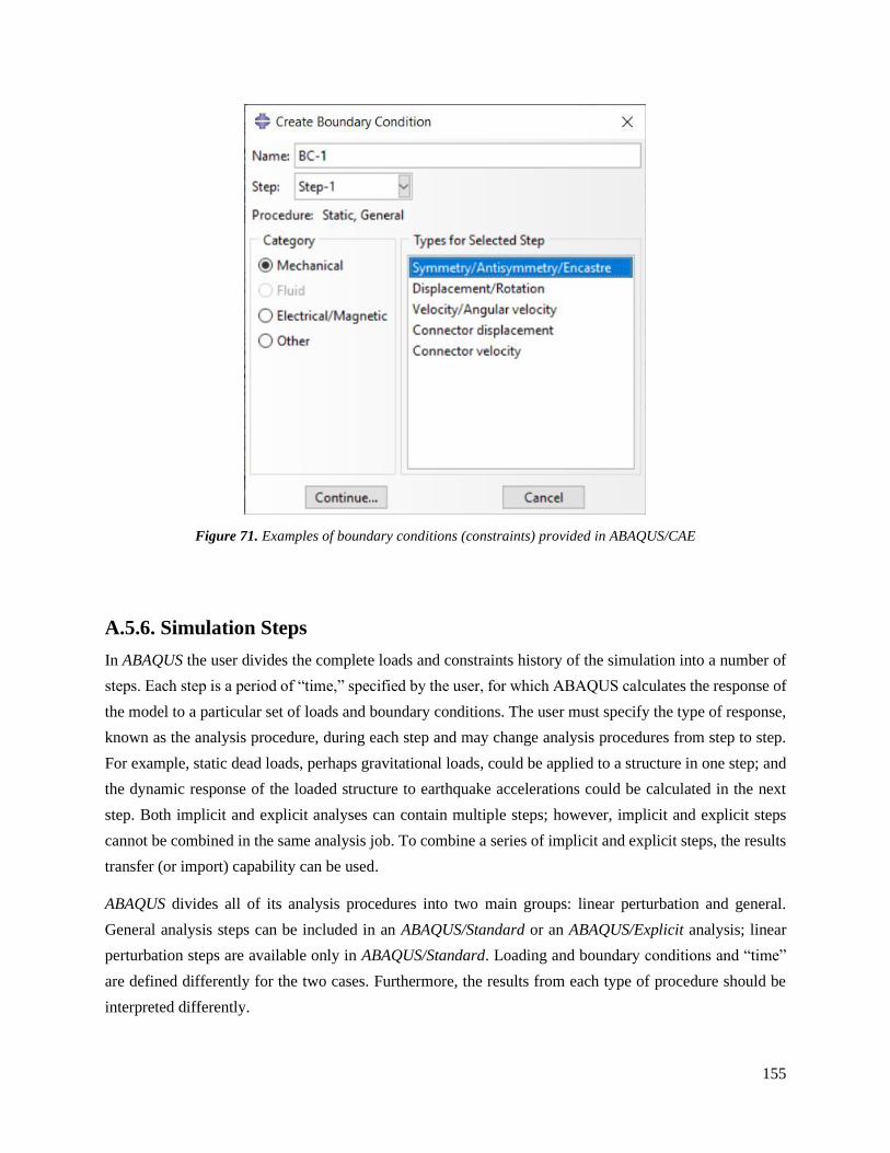
155
Figure 71. Examples of boundary conditions (constraints) provided in ABAQUS/CAE
A.5.6. Simulation Steps
In ABAQUS the user divides the complete loads and constraints history of the simulation into a number of
steps. Each step is a period of “time,” specified by the user, for which ABAQUS calculates the response of
the model to a particular set of loads and boundary conditions. The user must specify the type of response,
known as the analysis procedure, during each step and may change analysis procedures from step to step.
For example, static dead loads, perhaps gravitational loads, could be applied to a structure in one step; and
the dynamic response of the loaded structure to earthquake accelerations could be calculated in the next
step. Both implicit and explicit analyses can contain multiple steps; however, implicit and explicit steps
cannot be combined in the same analysis job. To combine a series of implicit and explicit steps, the results
transfer (or import) capability can be used.
ABAQUS divides all of its analysis procedures into two main groups: linear perturbation and general.
General analysis steps can be included in an ABAQUS/Standard or an ABAQUS/Explicit analysis; linear
perturbation steps are available only in ABAQUS/Standard. Loading and boundary conditions and “time”
are defined differently for the two cases. Furthermore, the results from each type of procedure should be
interpreted differently.

156
The response of the model during a general analysis procedure, known as a general step, may be either
nonlinear or linear. In a step that uses a perturbation procedure, which is called a perturbation step, the
response can only be linear. ABAQUS/Standard treats such steps as a linear perturbation about the
preloaded, predeformed state (known as the base state) created by any previous general steps; therefore, its
capability for doing linear simulations is rather more general than that of a purely linear analysis program.
In the case of general analysis, the starting point for each general step is the deformed state at the end of
the last general step. Therefore, the state of the model evolves in a sequence of general steps as it responds
to the loads defined in each step. Any specified initial conditions define the starting point for the first general
step in the simulation. All general analysis procedures share the same concepts for applying loads and
defining “time.”
Linear perturbation analysis steps are available only in ABAQUS/Standard, they calculate the linear
response of the structure to a perturbation load. The starting point for a linear perturbation step is called the
base state of the model. If the first step in a simulation is a linear perturbation step, the base state is the state
of the model specified using initial conditions. Otherwise, the base state is the state of the simulation at the
end of the last general step prior to the linear perturbation step. If another general step follows a perturbation
step, it uses the state of the model at the end of the last general step as its starting point, not the state of the
model at the end of the perturbation step. Thus, the response from a linear perturbation step has no
permanent effect on the simulation. Therefore, ABAQUS/Standard does not include the step time of linear
perturbation steps in the total time for the analysis. In fact, what ABAQUS/Standard actually does is to
define the step time of a perturbation step to be very small (10–36) so that it has no effect when it is added
to the total accumulated time. The exception to this rule is the modal dynamics procedure.