Design and implementation of a wire array antenna analyzer

Hrafnkell Eiriksson

March 5, 2000

Abstract

Design and implementation of a wire array antenna analyzer is discussed. The analyzer is based on theMethod of Moments and implemented in C++. Object-oriented design methods are used to make the soft-ware as general as possible and to allow for extensions. Implementation of numerical algorithms needed tosolve the problem are discussed.

Contents

1 Introduction 2

2 Theory 32.1 Currents on a dipole . . . . . . . . . . . . . . . . . . . . . . . . . . . . . . . . . . . . . . . 3

2.1.1 The applied field . . . . . . . . . . . . . . . . . . . . . . . . . . . . . . . . . . . . 42.2 Hallens integral equation . . . . . . . . . . . . . . . . . . . . . . . . . . . . . . . . . . . . 42.3 Hallens integral equation for arrays . . . . . . . . . . . . . . . . . . . . . . . . . . . . . . . 52.4 The farfield radiation pattern . . . . . . . . . . . . . . . . . . . . . . . . . . . . . . . . . . 6

3 Numerical methods 73.1 Method of Moments . . . . . . . . . . . . . . . . . . . . . . . . . . . . . . . . . . . . . . 7

3.1.1 Testing . . . . . . . . . . . . . . . . . . . . . . . . . . . . . . . . . . . . . . . . . 73.2 Solving Hallens integral equation for a dipole with the Method of Moments . . . . . . . . . 83.3 Solving Hallens integral equation for an array . . . . . . . . . . . . . . . . . . . . . . . . . 93.4 Using a triangle as a basis function . . . . . . . . . . . . . . . . . . . . . . . . . . . . . . . 93.5 Calculating the farfield pattern . . . . . . . . . . . . . . . . . . . . . . . . . . . . . . . . . 10

4 Results 11

5 Design of the software 125.1 The concept of object oriented programming . . . . . . . . . . . . . . . . . . . . . . . . . . 125.2 An object oriented array analyzer . . . . . . . . . . . . . . . . . . . . . . . . . . . . . . . . 12

5.2.1 C++ implementation details . . . . . . . . . . . . . . . . . . . . . . . . . . . . . . 13

A Numerical algorithms 16A.1 LU factorization . . . . . . . . . . . . . . . . . . . . . . . . . . . . . . . . . . . . . . . . . 16A.2 Simpson’s rule of integration . . . . . . . . . . . . . . . . . . . . . . . . . . . . . . . . . . 17

1

1 Introduction

This report documents the design and implementation of a wire array antenna analyzer. The mathematicaltheory on which it is based is presented and the integral equation that describes the currents on the wiresof the array is derived. A numerical method, the method of moments, for solving the integral equationis presented. The moment of methods is based on expanding the current on the wires with a set of basisfunctions. Results from using different expansion functions are compared.

The array analyzer is implemented in C++ and its object oriented design is presented. Finally anoverview of the numerical algorithms used in the program is given.

2

2 Theory

It is a well known fact that time varying currents radiate. When the currents and boundary conditions of theelectromagnetic problem to be solved are known both the electric and magnetic fields can be found. This isusually done with the help of the vector potential [Col85]. The current density and the vector potential arerelated as follows

A(r) =

ZVJ(r)

exp(jk0jr r0j)

4jr r0jdV 0 (1)

From that the H and E field can be found as

H(r) =1

rA(r) (2)

E(r) = j!A(r) +rr A(r)

j!(3)

2.1 Currents on a dipole

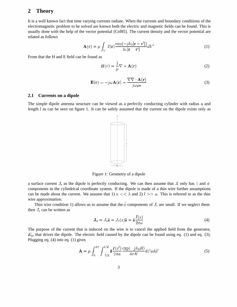
The simple dipole antenna structure can be viewed as a perfectly conducting cylinder with radius a andlength l as can be seen on figure 1. It can be safely assumed that the current on the dipole exists only as

2a

l

z

Figure 1: Geometry of a dipole

a surface current Js as the dipole is perfectly conducting. We can then assume that Js only has z and components in the cylindrical coordinate system. If the dipole is made of a thin wire further assumptionscan be made about the current. We assume that 1) a << and 2) l >> a. This is referred to as the thinwire approximation.

Thin wire condition 1) allows us to assume that the components of Js are small. If we neglect themthen Js can be written as

Js = Jsz = Js(z)z = zI(z)

2a(4)

The purpose of the current that is induced on the wire is to cancel the applied field from the generator,Eg, that drives the dipole. The electric field caused by the dipole can be found using eq. (1) and eq. (3).Plugging eq. (4) into eq. (1) gives

A =

Z 2

0

Z l=2

l=2zI(z0)

2a

exp(jk0R)

4Rdz0ad0 (5)

3

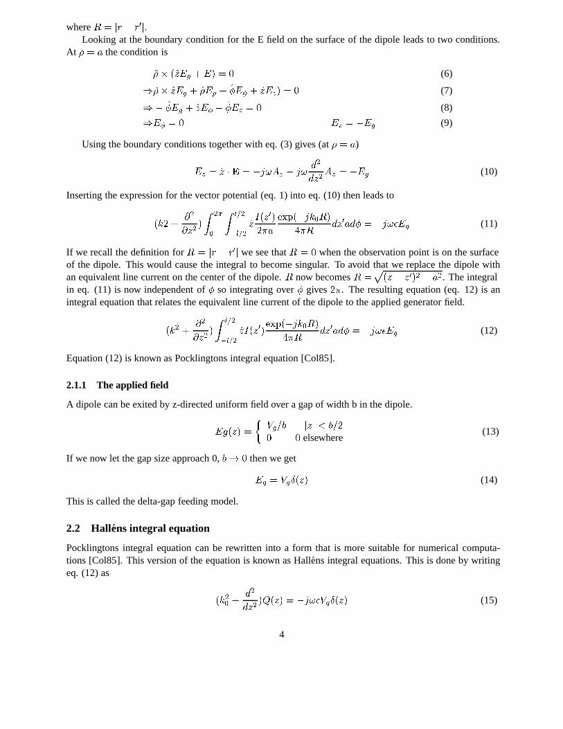
where R = jr r0j.Looking at the boundary condition for the E field on the surface of the dipole leads to two conditions.

At = a the condition is

(zEg +E) = 0 (6)

) zEg + E + E + zEz) = 0 (7)

) Eg + zE Ez = 0 (8)

)E = 0 Ez = Eg (9)

Using the boundary conditions together with eq. (3) gives (at = a)

Ez = z E = j!Az j!d2

dz2Az = Eg (10)

Inserting the expression for the vector potential (eq. 1) into eq. (10) then leads to

(k2 +@2

@z2)

Z 2

0

Z l=2

l=2zI(z0)

2a

exp(jk0R)

4Rdz0ad = j!Eg (11)

If we recall the definition for R = jr r0j we see that R = 0 when the observation point is on the surfaceof the dipole. This would cause the integral to become singular. To avoid that we replace the dipole withan equivalent line current on the center of the dipole. R now becomes R =

p(z z0)2 + a2. The integral

in eq. (11) is now independent of so integrating over gives 2. The resulting equation (eq. 12) is anintegral equation that relates the equivalent line current of the dipole to the applied generator field.

(k2 +@2

@z2)

Z l=2

l=2zI(z0)

exp(jk0R)

4Rdz0ad = j!Eg (12)

Equation (12) is known as Pocklingtons integral equation [Col85].

2.1.1 The applied field

A dipole can be exited by z-directed uniform field over a gap of width b in the dipole.

Eg(z) =

Vg=b jzj < b=20 0 elsewhere

(13)

If we now let the gap size approach 0, b! 0 then we get

Eg = VgÆ(z) (14)

This is called the delta-gap feeding model.

2.2 Hallens integral equation

Pocklingtons integral equation can be rewritten into a form that is more suitable for numerical computa-tions [Col85]. This version of the equation is known as Hallens integral equations. This is done by writingeq. (12) as

(k20 +d2

dz2)Q(z) = j!VgÆ(z) (15)

4

where

Q(z) =

Z l=2

l=2I(z0)

exp(jk0R)

4Rdz0: (16)

The solution to the differential equation eq. (16) is

Q(z) = A cos k0z jVgY02

sink0jzj (17)

where A and B are unknown constants. This is Hallens integral equation. By solving this equation thecurrent distribution on the dipole can be found. From the current distribution the radiated E and H field canbe found with the help of equations (1), (2) and (3).

2.3 Hallens integral equation for arrays

z

x

l l1 2

d

2az 2

1

V V21

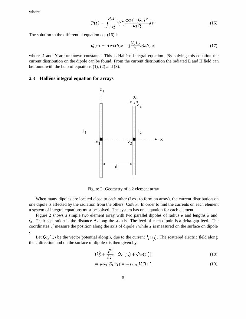
Figure 2: Geometry of a 2 element array

When many dipoles are located close to each other (f.ex. to form an array), the current distribution onone dipole is affected by the radiation from the others [Col85]. In order to find the currents on each elementa system of integral equations must be solved. The system has one equation for each element.

Figure 2 shows a simple two element array with two parallel dipoles of radius a and lengths l1 andl2. Their separation is the distance d along the x axis. The feed of each dipole is a delta-gap feed. Thecoordinates z0i measure the position along the axis of dipole i while zi is measured on the surface on dipolei.

Let Qij(zi) be the vector potential along zi due to the current Ij(z0j). The scattered electric field alongthe z direction and on the surface of dipole i is then given by

(k20 +@2

@z2i) [Qi1(zi) +Qi2(zi)] (18)

= j!Ei(zi) = j!ViÆ(zi) (19)

5

The system of equations can now be cast into a Hallen like equation the same way as was done above.This gives for the two dipole case

Q11(z1) +Q12(z1) =jk0Y0

2V1 sink0jz1j+C1 cos k0z1 (20)

Q21(z2) +Q22(z2) =jk0Y0

2V2 sink0jz2j+C2 cos k0z2 (21)

The vector potential functions are given by

Qij(zi) =

Z lj=2

lj=2

exp(jk0Rij)

4Rijdz0j (22)

where Rij is the distance from the observation point on dipole j to the integration point on dipole i.The extension of this to more than 2 parallel dipoles is obvious.

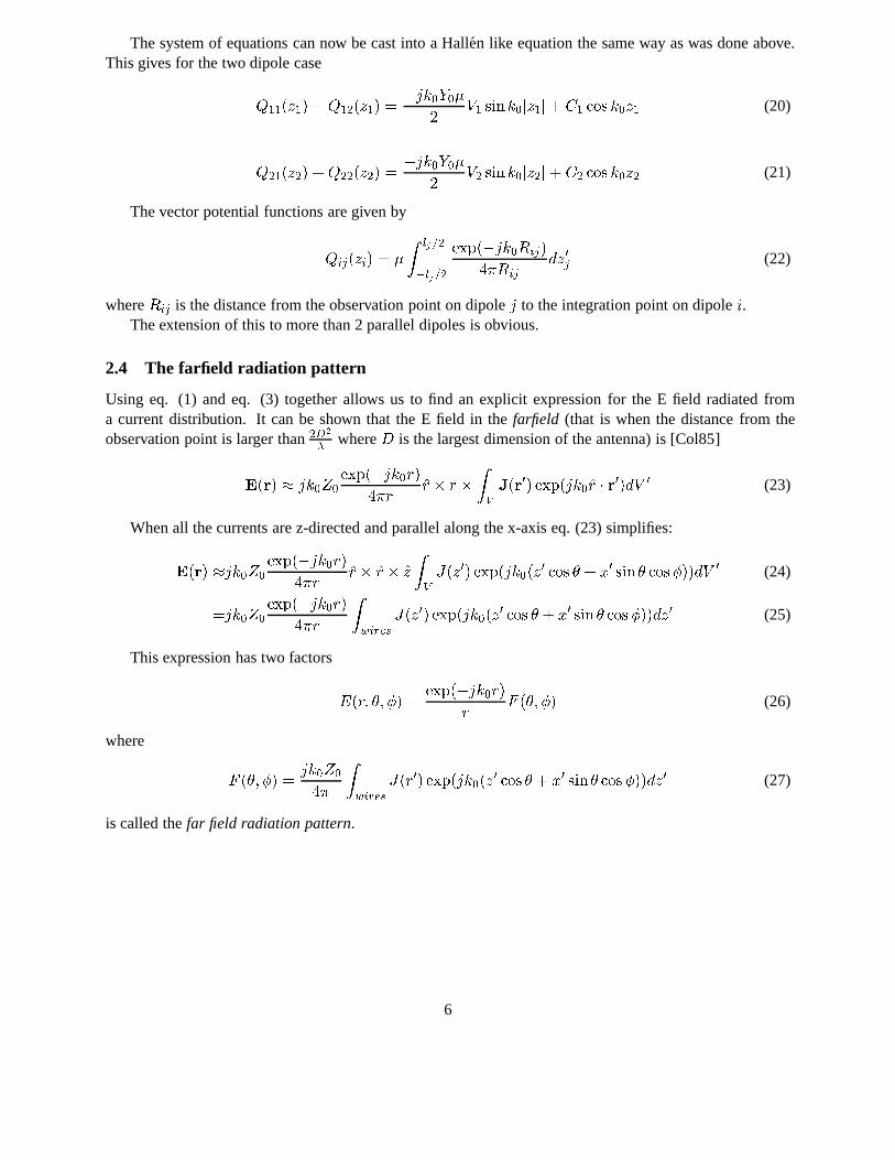
2.4 The farfield radiation pattern

Using eq. (1) and eq. (3) together allows us to find an explicit expression for the E field radiated froma current distribution. It can be shown that the E field in the farfield (that is when the distance from theobservation point is larger than 2D2

where D is the largest dimension of the antenna) is [Col85]

E(r) jk0Z0exp(jk0r)

4rr r

ZVJ(r0) exp(jk0r r

0)dV 0 (23)

When all the currents are z-directed and parallel along the x-axis eq. (23) simplifies:

E(r) jk0Z0exp(jk0r)

4rr r z

ZVJ(z0) exp(jk0(z

0 cos + x0 sin cos))dV 0 (24)

=jk0Z0exp(jk0r)

4r

Zwires

J(z0) exp(jk0(z0 cos + x0 sin cos))dz0 (25)

This expression has two factors

E(r; ; ) =exp(jk0r)

rF (; ) (26)

where

F (; ) =jk0Z0

4

Zwires

J(r0) exp(jk0(z0 cos + x0 sin cos))dz0 (27)

is called the far field radiation pattern.

6

3 Numerical methods

Hallens integral equation presented in section 2.2 can not be solved analytically. Numerical methods mustbe used. The most commonly used method for solving integral equations is the method of moments. Themethod is based on expanding the unknown current (or currents) with a set of basis functions and using thatto transform the integral to a sum.

3.1 Method of Moments

An integral equation like eq. (12) can be transformed into the equation

Z b

aG(z; z0)I(z0)dz0 = f(z) (28)

where f(z) has the domain [a; b] as its support. I(z) is the unknown and G(z; z0) is a kernel func-tion [Col85].

The current in the integral can be written as a sum of weighted basis functions

I(z) =

1Xn=1

Inn(z): (29)

When the expansion of the current (eq. (29)) is inserted into eq. (28) the integral is transformed into a sum:

1Xn=1

In

Z b

aG(z; z0)n(z

0)dz0 = (30)

1Xn=1

InGn(z) = f(z) (31)

where

Gn(z) =

Z b

aG(z; z0)n(z

0)dz0 (32)

The set of basis functions fn(z)g1n=1 is infinite and the equality in eq. (31) holds in some sense (f.ex.least squares, dependent on the basis chosen). In order to be able to work with eq. (31) in a computer wemust truncate the sum and choose to use only N basis functions. The equality in eq. (31) now becomes anapproximation. An error r(z) can be defined as

r(z) = f(z)NXn=1

InGn(z) (33)

3.1.1 Testing

Equation (31) is still a function of the variable z that has a continuous support domain. In order to be ableto work with it in a computer it has to be made discrete (or sampled). We can define a sampling grid with Npoints zm over [a; b] and force the error to be r(z) = 0 on that grid. We then get

NXn=1

InGn(zm) = f(zm) (34)

7

Forcing r(z) to be zero in N discrete points is often referred to as point testing or point matching.Equation (34) can be written as linear equation system

[Gnm]I = f (35)

where [Gnm] is a matrix with the elements Gn(zm), I is a column vector with the current weights In andf is a column vector with the elements f(zm). This system of linear equations can now be solved withGaussian elimination or LU factorization.

3.2 Solving Hallens integral equation for a dipole with the Method of Moments

Hallens integral equation has a similar form as eq. (28).Z l=2

l=2I(z0)

exp(jk0R)

4Rdz0 = A cos k0z j

VgY02

sink0jzj (36)

Here exp(jk0R)4R is the kernel.

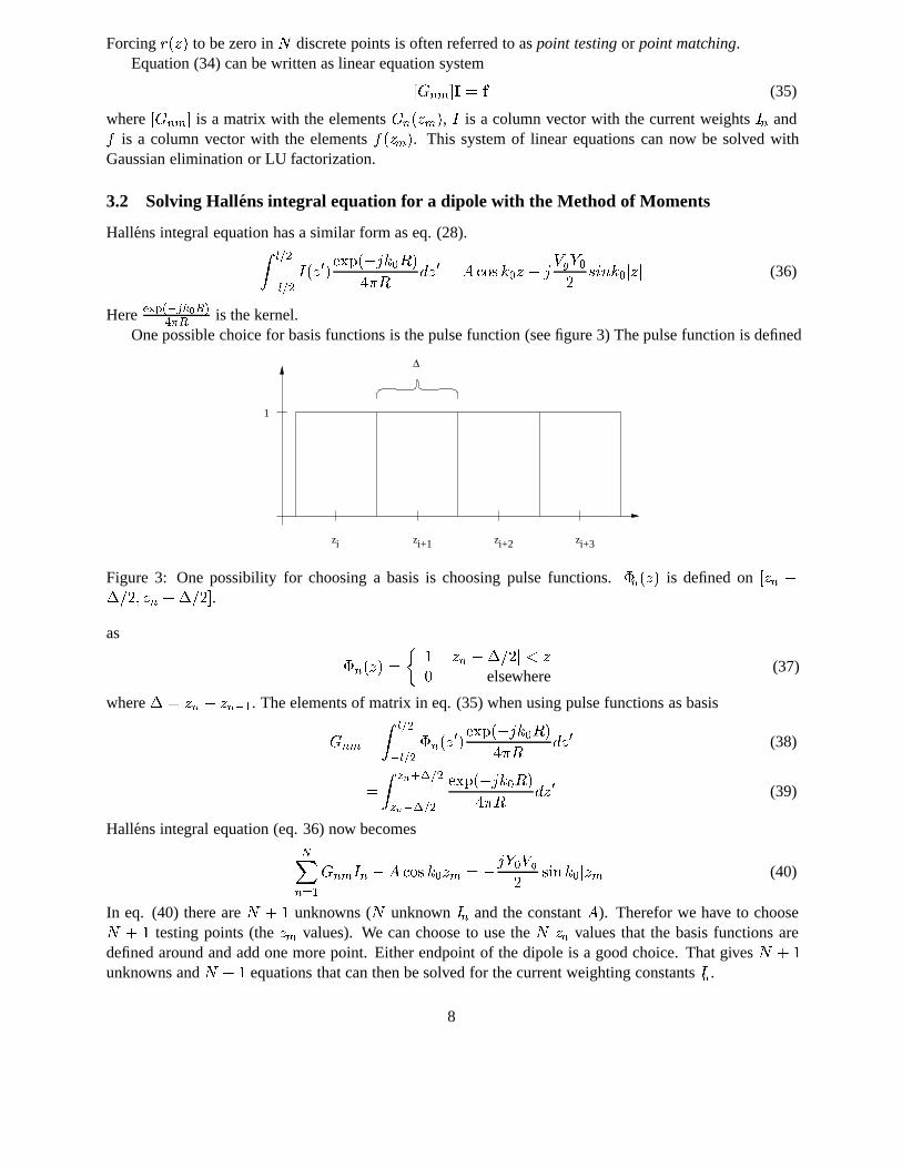
One possible choice for basis functions is the pulse function (see figure 3) The pulse function is defined

zi zi+1 zi+2 zi+3

∆

1

Figure 3: One possibility for choosing a basis is choosing pulse functions. n(z) is defined on [zn =2; zn +=2].

as

n(z) =

1 jzn =2j < z0 elsewhere

(37)

where = zn zn1. The elements of matrix in eq. (35) when using pulse functions as basis

Gnm =

Z l=2

l=2n(z

0)exp(jk0R)

4Rdz0 (38)

=

Z zn+=2

zn=2

exp(jk0R)

4Rdz0 (39)

Hallens integral equation (eq. 36) now becomes

NXn=1

GnmIn A cos k0zm = jY0Vg2

sink0jzmj (40)

In eq. (40) there are N + 1 unknowns (N unknown In and the constant A). Therefor we have to chooseN + 1 testing points (the zm values). We can choose to use the N zn values that the basis functions aredefined around and add one more point. Either endpoint of the dipole is a good choice. That gives N + 1unknowns and N + 1 equations that can then be solved for the current weighting constants In.

8

3.3 Solving Hallens integral equation for an array

Hallens integral equation for arrays (eq. (20) and (21) for the two element case) can be solved using themethod of moments in a way similar to what was done for the single dipole. Each Qij(z) becomes a blockin the matrix [Gnm] and the currents on the wires are represented in a single vector. Equations (20) and (21)become

N1Xn=1

G11nmI1n +

N2Xn=1

G12nmI2n A1 cos k0z1m = jY0V1g

2sink0jz1mj (41)

N1Xn=1

G21nmI1n +

N2Xn=1

G22nmI2n A2 cos k0z1m = jY0V2g

2sink0jz2mj (42)

where

Gijnm =

Z zn+=2

zn=2

exp(jk0Rij)

4Rijdz0 (43)

Ni is the number of basis functions needed (often also referred to as number of subdomains) on wire i ofthe array and Vig is the generator voltage for the i-th element

Equations (41) and (42) can be written up as a single system of linear equations as described above. Theresulting matrix equation will have the structure shown below

[G11] [cos k0z1m] [G12] [0]G21 [0] [G22] [cos k0z2m]

2664I1nA1

I2nA2

3775 =

jY02

V1g sink0jz1mjV2g sink0jz2mj

(44)

Extending this for more elements is obvious.

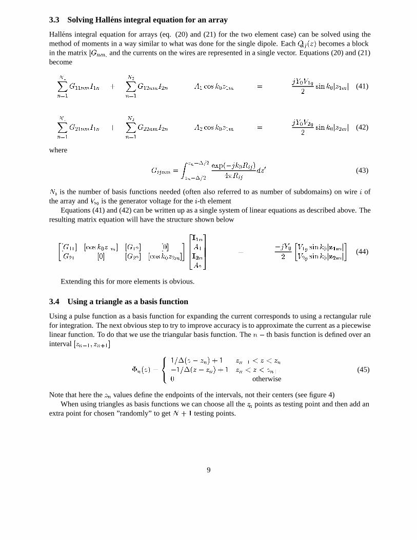
3.4 Using a triangle as a basis function

Using a pulse function as a basis function for expanding the current corresponds to using a rectangular rulefor integration. The next obvious step to try to improve accuracy is to approximate the current as a piecewiselinear function. To do that we use the triangular basis function. The n th basis function is defined over aninterval [zn1; zn+1]

n(z) =

8<:

1=(z zn) + 1 zn1 < z < zn1=(z zn) + 1 zn < z < zn+10 otherwise

(45)

Note that here the zn values define the endpoints of the intervals, not their centers (see figure 4)When using triangles as basis functions we can choose all the zn points as testing point and then add an

extra point for chosen ”randomly” to get N + 1 testing points.

9

Figure 4: The triangular basis functions. Note that the functions span two intervals and the functions at theends are different form the other.

3.5 Calculating the farfield pattern

When the currents on an wire array have been found its relatively easy to calculate the farfield radiationpattern from eq. (27). One can chose to do it numerically using an numerical integration method likeSimpson’s rule of integration (see Appendix A.2). When using simple basis functions as the pulse theintegration can be carried out analytically. When using pulse basis functions equation (27) becomes

F (; ) =

NwiresXn=1

[exp(jk0xn sin cos)

k0 cos2 sin(jk0=2 cos )

NsubdXm=1

Im exp(jk0zm cos)] (46)

10

4 Results

100

101

102

103

104

−50

0

50

100

150

200Convergence of input impedance of a dipole

Number of expansion functions per wavelength

Ω

Triangular − realTriangluar − imagPulse − real Pulse − imag

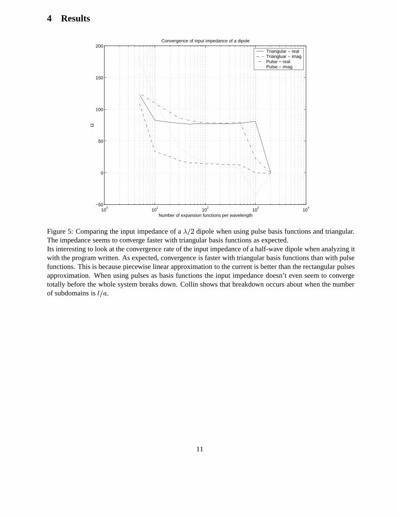
Figure 5: Comparing the input impedance of a =2 dipole when using pulse basis functions and triangular.The impedance seems to converge faster with triangular basis functions as expected.Its interesting to look at the convergence rate of the input impedance of a half-wave dipole when analyzing itwith the program written. As expected, convergence is faster with triangular basis functions than with pulsefunctions. This is because piecewise linear approximation to the current is better than the rectangular pulsesapproximation. When using pulses as basis functions the input impedance doesn’t even seem to convergetotally before the whole system breaks down. Collin shows that breakdown occurs about when the numberof subdomains is l=a.

11

5 Design of the software

5.1 The concept of object oriented programming

Using an object oriented programming language provides the programmer with some very powerful tools tohelp him organize his program [Str97].

One of the basic concepts in object oriented programming (OOP) is the class. A class is an representationof a concept, it is a collection of the data needed to represent its state and the operations (functions, methods)that can be applied to the data. The operations form the interface of the class.

Organizing classes into a hierarchy is another of the basic ideas in object oriented programming. At thetop of the class hierarchy is the most general representation of the idea or concept being implemented andfurther down are special versions of the concept. An example could be the basic class ”shape” and furtherdown in the hierarchy there might be a ”circle”. We say that the circle class is inherited from the ”shape”class. The ”shape” and the ”circle” class share the same interface. One possible operation to be applied to a”shape” would be to draw it.

When writing object oriented code it is important to remember to a) program to an interface, not animplementation and b) premature optimization is the root of all evil.

5.2 An object oriented array analyzer

The result of applying the moment of methods to an antenna array problem as described in section 2 arethe currents on each wire. What the currents are depends on the geometry of the problem (thickness, lengthand position of wires). It seems to be a good idea to represent an antenna array as a class that can be askedwhat the currents on its wires are. Someone who only wants to use the array analyzer doesn’t care how itsinternals are, he only wants to be able to a) specify the geometry to be analyzed and b) ask what the currentson the wires are. This makes up the interface of the general array analyzer class. Using different basisfunctions to expand the current can be represented by inherited classes from the basic array analyzer class.This is very convenient when exploring the different results when using different methods for calculating. Itallows the programmer to gather the implementation details that are common to all array analyzers into thebase class (f.x. to read in geometrical information) and only change the small details that are to be exploredin the derived classes.

Every array analyzer that uses the method of moments to analyze the currents on its wires has to do verysimilar things internally. It has to solve the matrix equation [Gnm]I = Vg . Before doing that it calculatesthe elements of the [Gnm] matrix and the Vg vector.

The matrix and vector are fundamental concepts used in finding the currents. They too can be repre-sented with a single class. A single matrix class is enough because vector can be considered a matrix wherethe number of columns or rows is 1. A matrix class has all the basic linear algebra functions such as solvinga system of linear equations. They form the interface of the matrix class.

To calculate the elements of the [Gnm] matrix, numerical integration must be used. One possible nu-merical algorithm is the Simpson rule of integration (see appendix A.2). The same numerical integrationmethod can be used to calculate the elements of the matrix independent on the choice of basis functions(and even kernels). The numerical integration method can therefor be implemented as class that representsan ”integration machine” that can integrate any function given to it. The integrator only has one operationin its interface: evaluate the given function.

One possible use of the currents found by the array analyzer is to calculate far field radiation patternfrom the antenna array. A far field calculator class could be constructed that has only one operation in itsinterface: give me the value of the far field pattern in the direction of (; ).

12

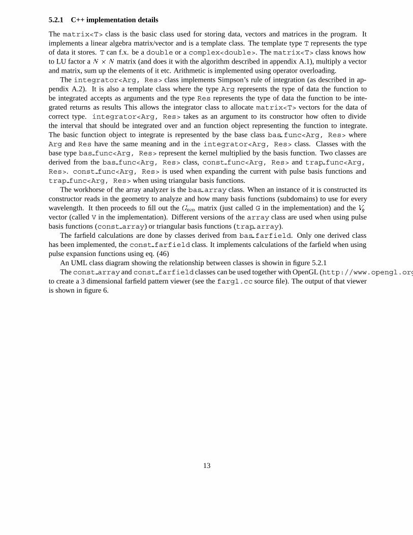
5.2.1 C++ implementation details

The matrix<T> class is the basic class used for storing data, vectors and matrices in the program. Itimplements a linear algebra matrix/vector and is a template class. The template type T represents the typeof data it stores. T can f.x. be a double or a complex<double>. The matrix<T> class knows howto LU factor a N N matrix (and does it with the algorithm described in appendix A.1), multiply a vectorand matrix, sum up the elements of it etc. Arithmetic is implemented using operator overloading.

The integrator<Arg, Res> class implements Simpson’s rule of integration (as described in ap-pendix A.2). It is also a template class where the type Arg represents the type of data the function tobe integrated accepts as arguments and the type Res represents the type of data the function to be inte-grated returns as results This allows the integrator class to allocate matrix<T> vectors for the data ofcorrect type. integrator<Arg, Res> takes as an argument to its constructor how often to dividethe interval that should be integrated over and an function object representing the function to integrate.The basic function object to integrate is represented by the base class bas func<Arg, Res> whereArg and Res have the same meaning and in the integrator<Arg, Res> class. Classes with thebase type bas func<Arg, Res> represent the kernel multiplied by the basis function. Two classes arederived from the bas func<Arg, Res> class, const func<Arg, Res> and trap func<Arg,Res>. const func<Arg, Res> is used when expanding the current with pulse basis functions andtrap func<Arg, Res> when using triangular basis functions.

The workhorse of the array analyzer is the bas array class. When an instance of it is constructed itsconstructor reads in the geometry to analyze and how many basis functions (subdomains) to use for everywavelength. It then proceeds to fill out the Gnm matrix (just called G in the implementation) and the Vgvector (called V in the implementation). Different versions of the array class are used when using pulsebasis functions (const array) or triangular basis functions (trap array).

The farfield calculations are done by classes derived from bas farfield. Only one derived classhas been implemented, the const farfield class. It implements calculations of the farfield when usingpulse expansion functions using eq. (46)

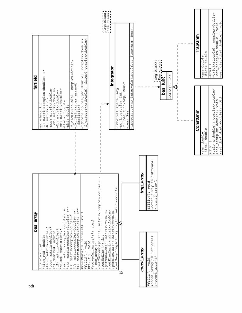
An UML class diagram showing the relationship between classes is showin in figure 5.2.1The const array and const farfield classes can be used together with OpenGL (http://www.opengl.org

to create a 3 dimensional farfield pattern viewer (see the fargl.cc source file). The output of that vieweris shown in figure 6.

13

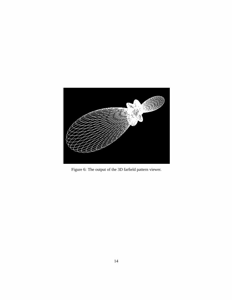
Figure 6: The output of the 3D farfield pattern viewer.

14

pth

bas

_arr

ay#no_elem: int

#elem_rad: double

#len: matrix<double>*

#pos: matrix<double>*

#dl_desired: double

#dl: matrix<double>*

#Nsubd: matrix<int>*

#ex: matrix<complex<double> >*

#zn: matrix<complex<double> >**

#G: matrix<complex<double>*

#V: matrix<complex<double> >*

#I: matrix<complex<double> >**

#readData(in:istream&): void

#fillG(): void

#fillV(): void

#solveCurrents()(): void

+~bas_array()

+getCurrents(n:int): matrix<complex<double> >

+getNoElem(): int

+getSubdLen(): matrix<double>

+getElemLen(): matrix<double>

+getElemPos(): matrix<double>

+getSamplingPoints(n:int): matrix<double>

con

st_a

rray

#fillG(): void

+const_array(in:istream&)

+~const_array()

trap

_arr

ay

#fillG(): void

+const_array(in:istream&)

+~const_array()

farf

ield

-no_elem: int

-I: matrix<complex<double> >*

-N: matrix<int>

-pos: matrix<double>

-len: matrix<double>

-dl: matrix<double>

-zn: matrix<double>*

-theta: double

-phi: double

-f_elem(x:double): complex<double>

+farfield(a:bas_array&)

+~farfield()

+f(theta:double,phi:double): complex<double>

+f_wrapper(x:double): friend complex<double>

bas

_fu

nc

+calc(): Res

Arg:class

Res:class

Co

nst

Gn

m-zm: double

-dist: double

+Gnm(:)

+calc(x:double): complex<double>

+set_testp(zm:double): void

+set_dist(dist:double): void

Tra

pG

nm

-zm: double

-dist: double

+Gnm(:)

+calc(x:double): complex<double>

+set_testp(zm:double): void

+set_dist(dist:double): void

inte

gra

tor

-interval_space: Arg

+no_intervals: int

-f: bas_func<Arg, Res>*

-res: Res

+integrator(no_intervals:int,f:bas_func<Arg, Res>)

Arg:class

Res:class

15

A Numerical algorithms

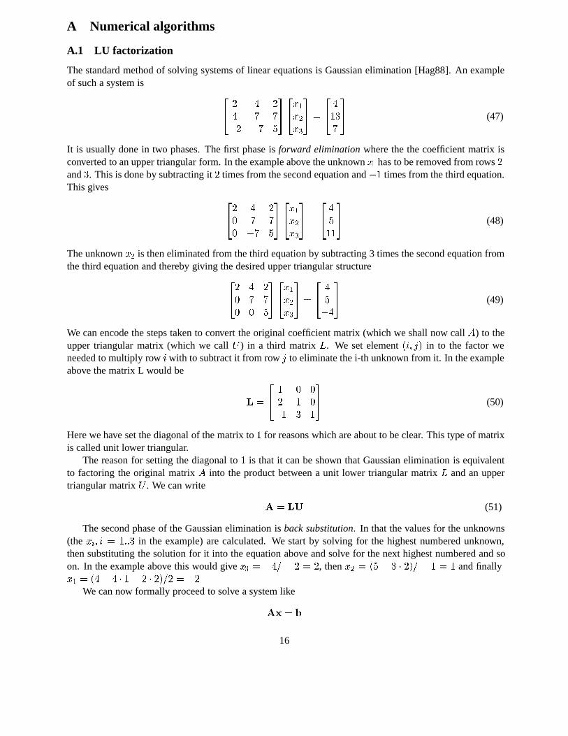
A.1 LU factorization

The standard method of solving systems of linear equations is Gaussian elimination [Hag88]. An exampleof such a system is

24 2 4 2

4 7 72 7 5

3524x1x2x3

35 =

24 4137

35 (47)

It is usually done in two phases. The first phase is forward elimination where the the coefficient matrix isconverted to an upper triangular form. In the example above the unknown x1 has to be removed from rows 2and 3. This is done by subtracting it 2 times from the second equation and 1 times from the third equation.This gives

242 4 20 7 70 7 5

3524x1x2x3

35 =

24 4511

35 (48)

The unknown x2 is then eliminated from the third equation by subtracting 3 times the second equation fromthe third equation and thereby giving the desired upper triangular structure

242 4 20 7 70 0 5

3524x1x2x3

35 =

24 4

54

35 (49)

We can encode the steps taken to convert the original coefficient matrix (which we shall now call A) to theupper triangular matrix (which we call U ) in a third matrix L. We set element (i; j) in to the factor weneeded to multiply row i with to subtract it from row j to eliminate the i-th unknown from it. In the exampleabove the matrix L would be

L =

24 1 0 0

2 1 01 3 1

35 (50)

Here we have set the diagonal of the matrix to 1 for reasons which are about to be clear. This type of matrixis called unit lower triangular.

The reason for setting the diagonal to 1 is that it can be shown that Gaussian elimination is equivalentto factoring the original matrix A into the product between a unit lower triangular matrix L and an uppertriangular matrix U . We can write

A = LU (51)

The second phase of the Gaussian elimination is back substitution. In that the values for the unknowns(the xi; i = 1::3 in the example) are calculated. We start by solving for the highest numbered unknown,then substituting the solution for it into the equation above and solve for the next highest numbered and soon. In the example above this would give x3 = 4= 2 = 2, then x2 = (5 3 2)= 1 = 1 and finallyx1 = (4 4 1 2 2)=2 = 2

We can now formally proceed to solve a system like

Ax = b

16

ht a b

x

f(x)

h

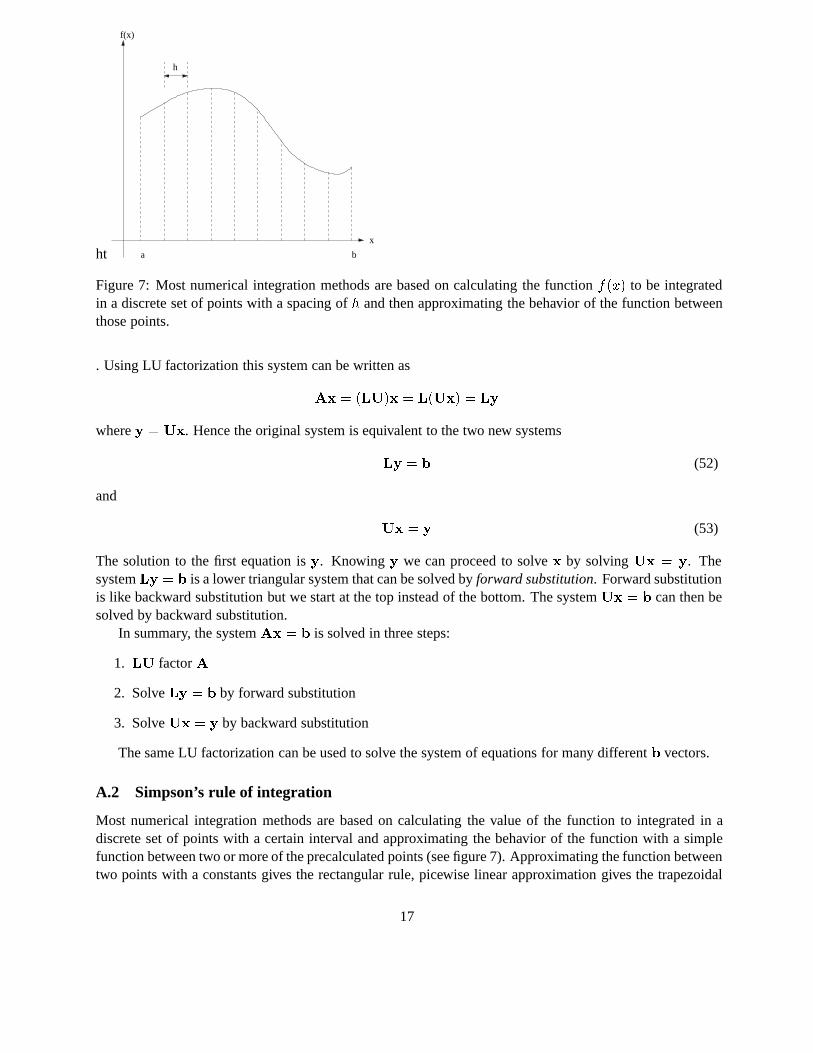
Figure 7: Most numerical integration methods are based on calculating the function f(x) to be integratedin a discrete set of points with a spacing of h and then approximating the behavior of the function betweenthose points.

. Using LU factorization this system can be written as

Ax = (LU)x = L(Ux) = Ly

where y = Ux. Hence the original system is equivalent to the two new systems

Ly = b (52)

and

Ux = y (53)

The solution to the first equation is y. Knowing y we can proceed to solve x by solving Ux = y. Thesystem Ly = b is a lower triangular system that can be solved by forward substitution. Forward substitutionis like backward substitution but we start at the top instead of the bottom. The system Ux = b can then besolved by backward substitution.

In summary, the system Ax = b is solved in three steps:

1. LU factor A

2. Solve Ly = b by forward substitution

3. Solve Ux = y by backward substitution

The same LU factorization can be used to solve the system of equations for many different b vectors.

A.2 Simpson’s rule of integration

Most numerical integration methods are based on calculating the value of the function to integrated in adiscrete set of points with a certain interval and approximating the behavior of the function with a simplefunction between two or more of the precalculated points (see figure 7). Approximating the function betweentwo points with a constants gives the rectangular rule, picewise linear approximation gives the trapezoidal

17

rule, and picewise quadratic approximation will give Simpson’s rule [Kre99]. Simpson’s rule is importantbecause it is sufficiently accurate for most problems, but still sufficiently simple.

To derive Simpsons rule we divide the interval of integration a x b into an even number, sayn = 2m, of equal subintervals of length h = (ba)=2m with endpoints x0(= a); x1; : : : ; x2m1; x2m(= b).We now take the first two subintervals and approximate f(x) in the interval x0 x x2 = x0 + 2h by theLagrange polynomial p2(x) through (x0; f(x0)),(x1; f(x1)),(x2; f(x2). The polynomial p2(x) is given as

p2(x) =(x x1)(x x2)

(x0 x1)(x0 x2)f(x0) + (54)

(x x0)(x x2)

(x1 x0)(x1 x2)f(x1) + (55)

(x x0)(x x1)

(x2 x0)(x2 x1)f(x2) (56)

The denominators are 2h2,h2 and 2h2, respectively. Setting s = (xx1)=h we have xx0 = (s+1)=h,x x1 = sh, x x2 = (s 1)=h and we obtain

p2(x) =1

2s(s 1)f(x0) (s+ 1)(s 1)f(x1) + (57)

1

2(s+ 1)sf(x2) (58)

We now integrate with respect to x from x0 to x2. This corresponds to integrating with respect to s from 1to 1. Since dx = hds the result isZ x2

x0

f(x)dx

Z x2

x0

p2(x)dx =h

3(f(x0) + 4f(x1) + f(x2)) (59)

A similar formula holds for the other intervals. By summing all these m formulas we obtain Simpson’s rule:

Z b

af(x)dx

h

3(f(x0) + 4f(x1) + 2f(x2) + 4f(x3) + (60)

+ 2f(x2m2) + 4f(x2m1 + f(x2m))) (61)

An algorithm for Simpson’s rule could then be:In: a, b, m, f0; : : : ; f2m Out: Approximate value of integral.Compute:

1. s0 = f0 + f2m

2. s1 = f1 + f3 + + f2m1

3. s2 = f2 + f4 + + f2m2

4. h = (b a)=2m

5. return h3 (s0 + 4s1 + 2s2)

18

References

[Col85] Robert E. Collin. Antennas and radiowave propagation. McGraw-Hill, 1985.

[Hag88] William W. Hager. Applied Numerical Linear Algebra. Prentice-Hall, 1988.

[Kre99] Erwin Kreyszig. Advanced Engineering Mathematics, 8th edition. John Wiley & Sons, 1999.

[Str97] Bjarne Stroustrup. The C++ Programming Language, third edition. Addison Wesley, 1997.

19