Embed Size (px)
Citation preview

DESIGN AND IMPLEMENTATION OF A HYBRID FACE RECOGNITION TECHNIQUE
__________________________
A Thesis
Presented to
the Faculty of the Elmer R. Smith College of Business and Technology
Morehead State University
_________________________
In Partial Fulfillment
of the Requirements for the Degree
Master of Science
_________________________
by
Asim S. Chaudhry
October 16, 2018

ProQuest Number:
All rights reserved
INFORMATION TO ALL USERSThe quality of this reproduction is dependent upon the quality of the copy submitted.
In the unlikely event that the author did not send a complete manuscriptand there are missing pages, these will be noted. Also, if material had to be removed,
a note will indicate the deletion.
ProQuest
Published by ProQuest LLC ( ). Copyright of the Dissertation is held by the Author.
All rights reserved.This work is protected against unauthorized copying under Title 17, United States Code
Microform Edition © ProQuest LLC.
ProQuest LLC.789 East Eisenhower Parkway
P.O. Box 1346Ann Arbor, MI 48106 - 1346
10980617
10980617
2018

Accepted by the faculty of the Elmer R. Smith College of Business and Technology, Morehead
State University, in partial fulfillment of the requirements for the Master of Science degree.
____________________________
Dr. Heba Elgazzar
Director of Thesis
Master’s Committee: ________________________________, Chair
Dr. Ahmad Zargari
_________________________________
Dr. Sam Nataraj
_________________________________
Dr. Cheng Cheng
________________________
Date

DESIGN AND IMPLEMENTATION OF A HYBRID FACE RECOGNITION TECHNIQUE
Asim S. Chaudhry
Morehead State University, 2018
Director of Thesis: __________________________________________________
Dr. Heba Elgazzar
The problem of face recognition is a subject that has been researched for many years. Face
recognition technology can be utilized in many different industries, it isn’t solely designated for
computer science relate fields. The purpose of this thesis is to continue this research and attempt
to provide a powerful classifier that works on par with the algorithms currently on the market.
This new algorithm will be known as the EFL Hybrid algorithm. This classifier is created by
combining many popular algorithms. There are three major algorithms that will be explored in
this thesis: Eigenfaces, Fisherfaces, and Local Binary Patterns Histograms. The Eigenfaces
algorithm utilizes Principal Component Analysis (PCA) to project the face data to a low
dimensional subspace where the data is distinct, and variation is maximized. These principal
components are called the eigenvectors or Eigenfaces. The Fisherfaces algorithm employs Linear
Discriminant Analysis (LDA) to reduce the dimensionality of the data. LDA projects the data
such that in between class and within class scatter is maximized. The Local Binary Patterns

Histogram (LBPH) is a classifier that uses texture descriptions based on local binary patterns
(LBP). A new image can be created by taking the LBP from each pixel in the original image.
This new LBP image is split up into blocks, each block is a histogram. These three algorithms
are tested against images provided by the Yale Face Database (Yale Face Database, n.d.). The
experimental results show that both the LBPH and Fisherfaces classifiers perform better than the
Eigenfaces classifier. Combining these three algorithms can provide the highest accuracy, as
long as the LBPH is ranked at the highest.
Accepted by: ______________________________, Chair
Dr. Ahmad Zargari
______________________________
Dr. Sam Nataraj
______________________________
Dr. Cheng Cheng

TABLE OF CONTENTS
CHAPTER I: INTRODUCTION ........................................................................................1
1.1 Background .......................................................................................................1
1.2 Facial Recognition Applications .......................................................................3
1.2.1 Security ...........................................................................................3
1.2.2 Law Enforcement ............................................................................4
1.2.3 Convenient Stores ...........................................................................4
1.2.4 Attendance ......................................................................................5
1.2.5 Identity Documents .........................................................................6
1.2.6 Disease Detection ............................................................................6
1.2.7 Assisting the Visually Impaired ......................................................7
1.3 Purpose ..............................................................................................................7
1.4 Objectives .........................................................................................................8
1.5 Limitations ........................................................................................................8
1.6 Definition of Terms .........................................................................................10
CHAPTER II: LITERATURE REVIEW .........................................................................10
2.1 Eigenfaces using PCA .....................................................................................10
2.2 Fisherfaces using LDA ...................................................................................11
2.3 Local Binary Patterns Histograms (LBPH) ....................................................13
2.4 Scale-Invariant Feature Transform (SIFT) .....................................................15
2.5 Speed-Up Robust Feature (SURF) ..................................................................15
2.6 Elastic Bunch Graph Matching .......................................................................16

CHAPTER III: METHODOLOGY ..................................................................................17
3.1 Tools ...............................................................................................................17
3.2 Software Libraries ...........................................................................................18
3.3 Data Preprocessing ..........................................................................................20
3.4 Algorithm Implementation ..............................................................................21
3.4.1 Eigenfaces Algorithm ............................................................................21
3.4.2 Fisherfaces Algorithm ............................................................................24
3.4.3 Local Binary Patterns Histogram Algorithm ......................................... 26
3.4.4 EFL Hybrid Algorithm ..........................................................................28
CHAPTER IV: EXPERIMENTAL RESULTS ................................................................30
4.1 Database for Face Recognition .......................................................................30
4.2 Eigenfaces Experimental Results ....................................................................31
4.3 Fisherfaces Experimental Results ...................................................................34
4.4 Local Binary Patterns Histograms Experimental Results ...............................37
4.4 EFL Hybrid Algorithm Experimental Results ................................................39
CHAPTER V: CONCLUSIONS ......................................................................................42
5.1 Summary .........................................................................................................42
5.2 Recommendations ...........................................................................................43
REFERENCES .................................................................................................................44

APPENDIX ......................................................................................................................48
Appendix A: Face Recognition Parent Class (Part 1) ..........................................48
Appendix B: Face Recognition Parent Class (Part 2) ..........................................49
Appendix C: Eigenfaces (Part 1) ..........................................................................50
Appendix D: Eigenfaces (Part 2) ..........................................................................51
Appendix E: Fisherfaces (Part 1) .........................................................................52
Appendix F: Fisherfaces (Part 2) .........................................................................53
Appendix G: Fisherfaces (Part 3) .........................................................................54
Appendix H: Local Binary Patterns Histograms (Part 1) ....................................55
Appendix I: Local Binary Patterns Histograms (Part 2) ......................................56
Appendix J: Local Binary Patterns Histograms (Part 3) .....................................57
Appendix K: Local Binary Patterns Histograms (Part 4) ....................................58
Appendix L: EFL Hybrid Algorithm .....................................................................59

CHAPTER I: INTRODUCTION
1.1 Background
Facial recognition is a technology that has been evolving steadily over the last decade. A skill
that is developed by children at a very young age has taken engineers years to develop. A child
will naturally develop his sight; however, a computer must be taught how to see. Giving a
computer the ability of sight is where the science of Computer Vision began. Gary Bradski
describes computer vision as, “the transformation of data from a still or video camera into either
a decision or a new representation” (Bradski, 2015, p. 18). An image by itself isn’t something
that a computer can comprehend, it needs to be translated to a different form. Everything a
computer understands is represented as a number, more specifically a binary number. A machine
tends to be most comfortable with numbers, so transforming the image into a group of numbers
is the most logical way to go.
Figure 1 shows how an image can be represented to allow a machine to understand it. Images
can be viewed as a matrix of numbers with each number representing a pixel in the image. In
terms of black and white images, these pixel numbers will represent the shades of gray of the
image. For a color picture each pixel is given three values. These three numbers represent the
level of red, green, and blue. The values range from 0 to 255 providing many different color
possibilities. Once the images are in number form they can be manipulated using tools such as
Machine Learning to help give machines the ability to perceive objects.

2
Figure 1: Image Representation in a Computer (Yale Face Database, n.d.)
Machine Learning is a programming implementation which allows a machine to learn a
specific pattern rather than having the pattern explicitly programmed into it. Mehmed Kantardzic
further explains that, “[Machine Learning] algorithms learn by searching through an n-
dimensional space of a given data set to find an acceptable generalization” (Kantardzic, 2011, p.
89). A computer can perform actions more rapidly and efficiently that a human being. It would
take a computer a fraction of the time to model complex data than it would for a human. It may
also find patterns that it’s human counterpart may never have discovered. There are two
important methods in Machine Learning: supervised learning and unsupervised learning. In a
supervised learning environment, the programmer provides data that serves as both the input and
the expected output. The machine would then perform its calculations on the data and obtain an
output. This output can then be compared to the expected output. What the programmer is doing
is teaching the machine based on examples. On the other hand, the unsupervised learning method

3
doesn’t rely on having an expected output. It is the machine’s responsibility to see how the data
fits together. Both of these methods can be effective depending on the requirements of the
project.
1.2 Facial Recognition Applications
Before the inner workings of face recognition technology can be discussed, it is important
to have an understanding as to why this technology is important. The reality is the use of face
recognition applications isn’t only isolated to the computer science industry. Face recognition
can provide many useful applications to all kinds of industries, from law enforcement to the
educational system. More specific applications will be discussed in this section.
1.2.1 Security
Face recognition technology can be used as another form of authentication when attempting
to access personal accounts. Whether that be personal computers, banking accounts, or even
email accounts having an extra layer of security can be invaluable when a person’s livelihood is
on the line. Automated Teller Machines (ATMs) already have cameras installed to help prevent
tampering. This camera can instead be used as a form of identification, only allowing the user to
access their account if their face is in the system. Securing this data behind a biometric security
system, such as face recognition, can be vital. Facial recognition is already being used as a form
of access control. Jeffrey S. Coffin developed a security method that uses face recognition to
identify individuals in order to determine their clearance access (Coffin, 1999). In the media,
biometric security measures are generally boiled down to retinal scans, and finger print scans.
Facial recognition is a very powerful biometric security system that can improve any access
system.

4
1.2.2 Law Enforcement
Law Enforcement is another industry that can benefit from facial recognition software. One
of the jobs required of policemen is tracking down criminals. Face recognition software can
automate this process by automatically tracking these criminals without needing any manpower
besides making the arrest. Cameras are set up all around the country, from traffic cameras, street
cameras, to private security cameras. The law enforcement officials can feed their database of
criminals into a facial recognition algorithm and use these cameras to track criminals all around
the world. Writing speeding tickets is another job police officers bog their time down with.
Sensors can be set up to check whether the car is going too fast. Then cameras can recognize the
face and automatically send a speeding ticket. Setting up cameras and speeding sensors may not
be very cost effective now; however, as technology progresses the cost of these things continue
to lower.
1.2.3 Convenient Stores
The police aren’t the only group that needs to track users. Convenient stores can even use
this technology to track customers throughout their stores. There are stores already employing
this technology, such as seven-eleven. Seven-eleven has applied a facial recognition system to
11,000 stores across Thailand allowing them to collect useful data by utilizing these functions
(Chan, 2018):
• identifying loyalty members
• analyzing in-store traffic
• monitoring product levels
• suggesting products to customers

5
• measuring the emotions of customers
Data is at a premium right now, companies such as Facebook are doing whatever they
can to collect as much data as possible from their users. In such a data driven society, this kind of
technology can bring a lot of growth to a company. With all this information being collected
from the customers, attempted thefts can be as trivial as looking through the cameras to see who
entered the store. Law enforcement can also provide these convenient stores with their criminal
database, so that the system can automatically alert the police if it spots a threat.
1.2.4 Attendance
The educational systems have some processes that can be improved by employing facial
recognition technology. Taking attendance is an important part of class time to ensure that all
students are present; however, the larger the class the more difficult and longer it takes to check.
The problem is compounded in classes that fill entire auditoriums. These systems, though not
used often, already exist. Abhishek Jha developed an automated attendance system that can
invaluable in the education industry (Jha, 2018). This system can help cut down the amount of
time needed in class by allowing the professor to jump straight into the material rather than waste
time calling everyone’s name one at a time. Many universities have already forgone the use of
attendance because sometimes it just isn’t feasible with the number of students they receive. By
automating this process, the university can track which students are attending lectures.

6
1.2.5 Identity Documents
Identity theft is a very serious issue that is prevalent in society. Adding another form of
security to identity documents can help prevent this kind of theft. Carlos Cobian Schroeder
developed a biometric security procedure that uses face recognition to combat identity theft
(Schroeder, 1998). All kinds of identity documents, such as passports and visas, can be backed
up by identity data which includes the person’s face. Computers are then set up to scan the
person’s face against the face in the system to authenticate the user. Faces can be unique, so it
would be difficult for a thief to gain access to an identity. There are reports that the Australian
Passport Office is creating a face recognition system. The system is designed to be used in online
government services, enabling the user to easily provide authentication (Lee, 2017). This is a
first step at employing this technology into the ecosystem, if it proves successful then it may
spread to other parts of the industry.
1.2.6 Disease Detection
Disease detection isn’t something most people would associate with facial recognition;
however, it is something that can be vastly improved by employing this technology. Paul
Kruszka and his colleagues developed a system that uses facial analysis technology to help assist
in early detection of the disease know as 22q11.2 deletion syndrome (Kruszka, 2017). This
disease is defined as a common microdeletion syndrome that is characterized by “congenital
heart disease, immunodeficiency, hypoparathyroidism, palatal, gastrointestinal, skeletal, and
renal abnormalities, characteristics facial features, developmental and speech delay and an
increased risk for psychiatric illness” (Kruszka, 2017, p.2). Early detection of this disease can
help the victims immensely.

7
1.2.7 Assisting the Visually Impaired
Face recognition software can be used to help blind people see. Of course, it won’t let them
literally see, but it can help them recognize people. It can be troublesome for a visually impaired
individual to recognize whomever they are currently speaking with in social settings. By
applying face recognition technology to this situation, the visually impaired can have more
enjoyable social interactions. This face recognition system can work by using a smart phone’s
built in camera. The phone would wirelessly transmit the face data to a remote server that
performs the recognition, and then transmits it back to the phone (Jafri, 2013). The phone can
then provide a sound queue based on the individual it classified, or even say the person’s name.
1.3 Purpose
Due to the increasing popularity of face recognition algorithms, it is important to have a
deeper understanding of how these algorithms work. This thesis will outline the process of
creating a facial recognition algorithm. Face recognition algorithms have been developed and
optimized for many years, it isn’t a new technology. There are many popular algorithms that
currently exist. The purpose of this thesis is to explore current algorithms and propose a hybrid
algorithm to improve the overall performance and provide better experimental results. The focus
of this study will be on three algorithms and these algorithms will be compared and analyzed. A
new hybrid algorithm is proposed that is based on the combination of these specific algorithms to
provide better experimental results.

8
1.4 Objectives
There are three main objectives for the proposed work in this thesis:
1. Implementing three facial recognition algorithms: Eigenfaces, Fisherfaces, and Local
Binary Patterns Histograms
2. Testing and analyzing the experimental results of these three algorithms
3. The creation of a new hybrid facial recognition algorithm that combines three algorithms
1.5 Limitations
Training a machine learning algorithm can take a great deal of data to achieve maximum
optimization and reduce error. Depending on the algorithm employed, these “learning” sessions
can take a very long time. The training sessions can put a great deal of stress on the computer, so
its imperative that a powerful computer is used. A computer with a stronger processor can handle
more calculations and operations in a lower amount of time. In the case of image processing, a
powerful graphics card can also be useful. The algorithms being explored in this project can take
some time; however, the dataset is small enough that training times could be lessened. For this
project, a high-quality computer is being used.

9
1.6 Definition of Terms
The following are definitions of terms that will be used extensively within this thesis.
Principal Component Analysis (PCA): Transformation of the dataset to a lower
dimensional set where most of the important information still exists (Kantardzic, 2011).
Linear Discriminant Analysis (LDA): A tool used to construct a discriminant function
providing different results when applying data from different classes. (Kantardzic, 2011).
Local Binary Patterns: A texture description operator that assigns a label to every pixel
of an image by thresholding the neighborhood of the pixel with the center value (Ahonen,
2006).
Training Set: The data set that is reserved for training the classifier.
Testing Set: The data set that is reserved for testing the results of a fully trained
classifier.
Confusion Matrix: A table that displays in-depth results of the algorithm’s performance
by comparing the predicted class to the actual class.

10
CHAPTER II: LITERATURE REVIEW
2.1 Eigenfaces using PCA
The first algorithm that will be implemented is the Eigenfaces classifier. For the purpose
of this thesis. it is important to discover what research has already been completed on this
subject. Eigenfaces is an algorithm that uses Principal Component Analysis. PCA is a data
reduction tool used for multivariate data. Kantardzic defines PCA as, “a method of transforming
the initial data set represented by vector samples into a new set of vector samples with derived
dimensions” (Kantardzic, 2011, p. 70-71). The theory behind using PCA is that the data is
projected to a subspace where there is maximum variance. This tool facilitates the transformation
of a larger data set into a smaller more manageable set which contains all the essential parts to
reduce the dimensionality. PCA is an unsupervised method, meaning it doesn’t require class
information (Rahman, 2012). Features, or eigenvectors, are extracted from a covariance matrix, a
matrix that holds the covariance for each data element.
Matthew Turk and Alex Pentland employed Principal Component Analysis in the
development of an algorithm called Eigenfaces (Turk, 1991). After applying PCA to the dataset,
they obtained the eigenvectors. Since vectors are in the form of 1xN, they need to be reformatted
before they can be viewed as Eigenfaces. Turk and Pentland found that you can represent an
individual face as a linear combination of Eigenfaces (Turk, 1991). Each Eigenface would be
multiplied by a constant or weight, and then the resulting values are summed up. This algorithm
was tested on a database with over 2500 images, 16 subjects, and each image had a resolution of
512x512. Turk and Pentland obtained an accuracy of 96% correct over lighting variation, 85%
correct over orientation variation, and 64% correct over size variation (Turk, 1991).
11
Another form of PCA exists as the Modular Principal Component Analysis algorithm.
This method involves splitting the image into sub images. After these images are split up, the
PCA steps are applied. These sub images are placed into a training set filled with other sub
images. A covariance matrix can then be computed from this new set of data, from which the
eigenvectors can be extracted. Ambika, Arathy and Srinivasa completed an experiment using
MPCA on their face data (D. Ambika, 2012). They tested this algorithm against three different
face databases: the ORL, JAFFE, and Indian databases. The ORL database provided them 40
distinct subjects, and the classifier had an accuracy of 99% (D. Ambika, 2012). The Indian
database also had 40 distinct subjects, giving an accuracy of 99% (D. Ambika, 2012). Finally,
the JAFFE database, providing 10 distinct subjects, had an accuracy of 99% (D. Ambika, 2012).
This is clearly a strong algorithm for face recognition.
2.2 Fisherfaces using LDA
The Fisherfaces algorithm differs from Eigenfaces in that it uses Linear Discriminant
Analysis. LDA involves “finding a set of weight values that maximizes the ratio of the between-
class to the within-class variance of the discriminant score for a preclassified set of samples”
(Kantardzic, 2011, p. 163). LDA is a classification model that was originally created by R. A.
Fisher in the article The Use of Multiple Measurements in Taxonomic Problems (Fisher, 1936).
Despite having its start in plant classification, this tool has applications in facial recognition.
LDA puts a bigger emphasis on the classes in the data. When the data is trained, the LDA
ensures that the separation in between different classes is maximized.
Peter N. Belhumeur explores the use of LDA in his Fisherfaces algorithm by comparing
its effectiveness to the Eigenfaces algorithm (Belhumeur, 1997). The Fisherface algorithm starts
with obtaining the between-class and within-class scatters for the data. A projection is created

12
from this data that maximizes the ratio of the two scatters (Belhumeur, 1997). From this
projection the eigenvectors are obtained. These vectors can then be reformatted into Fisherfaces.
Belhumeur compared the results from his Eigenfaces algorithm which obtained an error rate of
24.4% to the results of his Fisherface algorithm, which obtained an error rate of 7.3%
(Belhumeur, 1997). An error rate of 7.3% is very impressive for a face recognition algorithm.
Another Fisherface experiment was completed by Mustamin Anggo and La Arapu
(Anggo, 2018). Following the algorithm proposed by Belhumeur, they created their own version
of the Fisherface classifier. This version followed the original structure of the Fisherface
algorithm very closely. After running the algorithm through their dataset, they arrived at an
accuracy of 93% (Anggo, 2018). This experiment provided an additional source of results from
a different face database.
Wenyi Zhao, in his paper, attempted to use only LDA in face recognition (Zhao 1998).
He found that this method doesn’t function properly. There are three cases where a pure LDA
face recognition classifier fails (Zhao 1998):
• The testing samples are from classes not present in the training set
• The testing samples are different from the data in the training set
• The samples have different backgrounds
He managed to solve this issue by employing PCA alongside LDA. He completed his
experiment on the FERET face database. The database contained 1316 training images from 526
classes and 298 testing images from 298 different classes. An accuracy of 95% was obtained
using this classifier (Zhao 1998).

13
2.3 Local Binary Patterns Histograms (LBPH)
Local Binary Patterns Histograms is a very simple and popular algorithm in facial analysis.
The LBP operator is highly discriminative. It’s invariance to monotonic gray-level changes and
efficiency allow it to be a powerful tool in facial analysis (Ahonen, 2006). A face can consist of
many of patterns that can make the LBP texture features invaluable in facial classification. LBP
can be used to describe both the texture and the shape of an image (Rahim, 2013). Timo Ahonen
and Matti Pietikainen present an experiment where they attempt to use local binary patterns in
facial recognition (Ahonen, 2006). Each pixel in the face image is given a new value based on
the values of the pixels in its ‘neighborhood’. Ahonen and Pietikainen define the neighborhood
as a 3x3 matrix around the original pixel (Ahonen, 2006). Once this LBP image is created it is
further subdivided into regions. These regions are then concatenated together into a large
histogram. This algorithm was run on the FERET database, which contains 14,051 gray-scale
images or 1,199 individuals and obtained an accuracy of 97%.
Abdur Rahim and his colleagues also implemented the Local Binary Patterns algorithm
(Rahim, 2013). They used LBP for face recognition by splitting it into three different parts: face
representation, feature extraction, and classification (Rahim, 2013). The face is first represented
as an LBP image, then the histograms are extracted. The classification phase is determined by
comparing histograms. Rahim explores three different methods of comparing histograms:
Histogram Intersection, Log-likelihood Statistic, and Chi square statistic (Rahim, 2013). The
image dataset contains images taken from either a camera or a face database. The classifier is fed
a total of 2000 total faces. 1980 of these faces are recognized, while 20 are unrecognized,
yielding an accuracy of 99% (Rahim, 2013).

14
There is a variation of this algorithm called the Local Gabor Binary Pattern Histogram
Sequence. This classifier is robust to variation of imaging conditions and has more
discrimination power (Zhang, 2005). The combination of Gabor filters and Local Binary Patterns
enhances the algorithm. Wenchao Zhang created a classifier using this method (Zhang, 2005).
He argues that the generalization obtained when training some of the popular algorithms is a
problem. He hopes to avoid these issues by completely forgoing the training stage. His algorithm
works in several steps (Zhang, 2005):
1. The input face is normalized.
2. Using Gabor filters, several Gabor Magnitude Pictures are obtained.
3. The Gabor Magnitude Pictures are converted to Local Gabor Binary Pattern images
4. The LGBP is subdivided into rectangle regions
5. Histograms are concatenated to form a total histogram
Zhang uses two approach to compare the histograms: direct matching and weighted matching
(Zhang, 2005). The direct matching method simply compares the histograms; on the other hand,
weighted matching applies a weight to regions of the face that are most important for
recognition. Zhang ran his classifier on the FERET face database and obtained an accuracy of
94% using the direct method, and 98% using the weighted method (Zhang, 2005).

15
2.4 Scale-Invariant Feature Transform (SIFT)
The Scale-Invariant Feature Transform algorithm is a useful tool in detecting and describing
feature points on an image. This algorithm was originally created for use in object detection;
however, it has transitioned into facial analysis. SIFT can extract gray-level features using local
patterns taken from a scale-space decomposition of the image (Bicego, 2006). As the name
suggests the features that are extracted from this algorithm are invariant, or never changing,
based on changes in the environment such as light and distortion making these very distinct
features. Manuele Bicego implemented this algorithm by comparing the SIFT features of the
input face to the training set (Bicego, 2006). He used three different techniques to identify the
correct face. These techniques were: calculating the distance between all the features to find the
minimum distance, matching the eyes and mouth features, and matching features based off their
grid (Bicego, 2006).
2.5 Speed-Up Robust Feature (SURF)
The creation of the Speed-Up Robust Features method was influenced by SIFT. Like SIFT,
this algorithm involves obtaining features that are invariant to changes in the environment. SURF
involves two important phases: detection and description. In the detection phase, important
points of interest are found on the image. In order to find these points of interest, blob-like
structures are located where the determinant is at maximum (Du, 2009). The description phase
describes the features using Haar Wavelets.

16
2.6 Elastic Bunch Graph Matching
The Elastic Bunch Graph Matching algorithm uses face graphs to model the data. This
classifier finds distinct local features of the face. It is inspired by biological processes in the
brain. One of these is the Gabor wavelet. Gabor wavelets can be defined as, “biologically
motivated convolution kernels in the shape of plane waves restricted by the Gaussian envelope
function” (Wiskott 1997, p.2). This feature is found to be a good model of early visual
processing in the brain (Wiskott 2014). The matching algorithm is also based on dynamic link
matching, a model of invariant object recognition in the brain (Wiskott 2014). Feature jets are
used to form a face graph. Jets can be defined as a small patch of gray values in an image around
a given pixel (Wiskott 1997). The face recognition process involves measuring the similarity of
the face graphs. Laurenz Wiskott utilized Elastic Bunch Graph Matching in her paper, using the
ARPA/ARL FERET database, to obtain an accuracy of 98% (Wiskott 1997).

17
CHAPTER III: METHODOLOGY
This section will present the methods for achieving the objectives presented in the
introduction of this thesis. The first objective is to implement three face recognition algorithms.
The procedure of implementing these algorithms is discussed in this chapter, as well as the
software libraries that will assist in programming the classifiers. The second object involves the
testing and analyzing of the three algorithms. Properly preprocessing the data is important so that
it can provide the best experimental results when employed in the algorithms. Tools and software
libraries are provided that will create tables and plots to help analyze the potential findings. The
last objective is to create a hybrid algorithm that combines the three algorithms that are already
implemented. The implementation of this EFL hybrid algorithm will be discussed in the final
section.
3.1 Tools
The face recognition algorithms implemented for this thesis are coded in their entirety
using Python. Python is a very useful language for applications in data science and machine
learning. It is very easy to use, while providing quite a bit of complexity. It also provides useful
tools for computer vision and machine learning through its many libraries which are included in
the Anaconda distribution. The Anaconda Python distribution is a platform that allows
organizations to develop machine learning and data science related projects (Anaconda, 2018).
Anaconda also provides as robust programming development environment called Spyder.
Combined with the Anaconda tools and Spyder editor all the tools necessary to complete this
project are provided for. Training this algorithm may take a lot of time depending on how
powerful of a machine is used. Fortunately, this project will run on a laptop which contains an

18
Intel® CoreTM i7-6700HQ processor accompanied by an NVIDIA GeForce GTX 1070 graphics
card. These tools will be integral to implementing the algorithms stated in the objectives.
3.2 Software Libraries
Python has access to many powerful libraries that will be imperative in the completion of
this project. One of these libraries is OpenCV. The Open Source Computer Vision (OpenCV)
library was created to provide a simple computer vision infrastructure that can help build
complex applications rapidly (Bradski, 2015). This library makes it easier and more convenient
to create powerful application in the computer vision domain. OpenCV provides over 500 useful
functions for many different areas of computer vision including (Bradski, 2015):
• Factory product inspection
• Medical imaging
• Security
• User interface
• Camera calibration
• Stereo vision
• Robotics
This library also provides invaluable functions to help with the creation of facial recognition
algorithms. For example, OpenCV comes equipped with a function that performs principal
component analysis on the data. This provides an easy method to extract eigenvectors from a set
of data. OpenCV was originally written in C and C++; however, they do maintain development
and maintenance on an interface for Python. OpenCV will provide shortcuts in the programming
that can help reduce the amount of coding time.

19
Another useful Python library that will be utilized is NumPy. This library provides a
powerful tool, the NumPy array, that is practically a standard in Python related data science. The
NumPy array can be described as a multidimensional, uniform collection of elements (Walt,
2011). These arrays can have any number of dimensions and a combination of many different
data types such as integers, Booleans, and strings (Walt, 2011). NumPy also contains many
useful functions for manipulating matrices. Some of these functions include: inverting matrices,
sorting vectors, and transposing vectors. These functions will be vital since the face data will be
stored in matrices.
The ability to view the images and craft charts is something that is invaluable in this project.
The matplotlib library provides tools to achieve these goals. Matplotlib is a python library
designed to help create plots of the data. This library was created to emulate graphics commands
that are already available in MATLAB™ (Hunter, 2007). This library complements greatly with
NumPy which provides access to highly powerful arrays. The data employed in this thesis is
almost entirely full of images. This library provides a useful tool to view these images and the
transformations applied on them.
Another powerful library used for machine learning is the scikit-learn library. This library
provides powerful tools for classification, regression, and clustering. While these tools are
useful, for the most part the face recognition program implemented in the thesis was coded from
scratch. The PCACompute() method from OpenCV is one of the exceptions. The scikit-learn
library is also useful because it provides excellent functions for testing algorithms. Its use in this
experiment is restricted to the use of the confusion matrix method. This method allows easy
creation of confusion matrices which are valuable in analyzing the experimental results.

20
3.3 Data Preprocessing
Before the data can be fed into a recognition algorithm, it must first be processed into the
proper form. Each specific algorithm has their own form of data processing; however, there are
some general transformations that can be completed for all of them. As stated previously, images
are stored as matrices where each entry represents a pixel. Each pixel contains three values
which can represent all the colors in the spectrum. The values are formatted as red, green, blue
(rgb). For the purposes of this algorithm, the actual color of the image is unimportant. The
algorithms used in this project will focus more on the color intensity rather than the actual colors.
To get the most out of the algorithms, grayscale images are used. A grayscale image represents
the data in shades of gray. Instead of having three values (rgb) for each pixel in the image matrix,
there is only one value which represents intensity of the gray. The database being used in the
project already has the images formatted as grayscale simplifying the data preprocessing steps.
The last step is to split the data into training and testing sets. The training set is what will be used
to train the algorithms. It is important to have many examples for every class in the training set.
The more data in the training set, the more accurate the classifier becomes. The testing set will
have the data that will be tested against the trained algorithm to determine its accuracy. For this
project, a 4:1 ratio of training to testing will be used to split up the data. It is important to make
sure that there is at least one instance of each class in the testing sample otherwise it would be
impossible to test all the classes.

21
3.4 Algorithm Implementation
One of the objectives is to implement three face recognition algorithms. In this section,
the implementations of each algorithm will be discussed. This thesis will explain the
implementation of three major face recognition algorithms: Eigenfaces, Fisherfaces and Local
Binary Pattern Histograms. These three algorithms will serve as the structure for the hybrid
algorithm which will provide improved experimental results over each of these components.
3.4.1 Eigenfaces Algorithm
Training an Eigenfaces algorithm involves obtaining the eigenvectors of the dataset, by
employing Principal Component Analysis, then calculating the weights for each face to perform
the recognition process. To perform PCA on the data, it must first be transformed into a vector
format. Given of a set of images X = {X1, X2, …, Xk} of dimensions NxM, the images must be
transformed to a vector form of 1x(N*M) (Turk, 1991). From this an entirely new table is created
where each row represents a face. At this point the data is ready to perform principal component
analysis upon. Its important to remove all the common features of the faces so that all the unique
features can remain (Turk, 1991). To achieve this, the mean face Ψ can be calculated using the
equation in by adding up all the face vectors Xi and dividing by the total number of faces k(1).
Ψ =1
𝑘∑ 𝑋𝑖
𝑘𝑖=1 (1)
Φ = 𝑋𝑖 − Ψ (2)
Each face is subtracted by the mean face leaving only the unique data as seen in the
equation, where Φ is the normalized face vector (2). Figure 2 displays what the average face

22
would look like. This face should look like a generic person with very little unique features.
Subtracting this face from the rest of the data set will in theory leave only distinct features.
Figure 2: Average Face of Training Set (Yale Face Database, n.d.)
From here the covariance matrix is ready to be computed. The covariance matrix can be
calculated by using equation (3), where C is the covariance matrix and Φ is the normalized face
vector . To multiply two vectors, one of them must first be transposed T. Eigenvectors will be
extracted from the covariance matrix. The eigenvectors are sorted by their eigenvalues, then the
top X number of components are extracted (Turk, 1991). Generally having a small number of
eigenfaces isn’t preferable.
𝐶 =1
𝑘∑ΦΦT (3)
OpenCV comes equipped with a function, called PCACompute(), which will complete
the PCA task and provide the user with the mean face and the eigenvectors. These eigenvectors

23
can be reshaped into their original forms and be viewed as a face. Each face in the training set
can be portrayed as a linear combination of these eigenfaces. Setting the number of components
from the PCA method to 15 will yield 15 eigenfaces. These 15 faces contain all the important
distinct features from the entire dataset. By applying a weight to each of these eigenfaces, any of
the faces in the training set can be recreated. At this point, weights are calculated for each face in
the dataset. Once all the weights are calculated, the algorithm is ready to start classifying faces.
The face recognition task is very similar to the training process. The input image must
first be flattened so that it fits the form of 1x(N*M). Next the mean face Ψ is subtracted from
this input vector to ensure that only unique features remain. The weights are then calculated for
the face, so that they can be portrayed as a linear combination of the Eigenfaces. Using
Euclidean distance, these weights are compared to the weights in the training set. The face with
the lowest Euclidean distance is deemed to be the same class as the input face. This algorithm
can be summed up by the flow chart provided in Figure 3.
Figure 3: Eigenfaces Flow Chart

24
3.4.2 Fisherfaces Algorithm
The Fisherfaces algorithm was developed as an improvement to the Eigenfaces
algorithm. This method uses Linear Discriminant Analysis to create Fisherfaces which represent
all the training data. One of the major differences between PCA and LDA is that PCA ignores
classes. LDA treats the data in a way such that same classes are clustered tightly together, while
different classes are as far away as possible from each other (Wagner, 2012).
Philipp Wagner supplied an implementation to Fisherfaces that proved very helpful in the
implementation of this algorithm (Wagner, 2012). This algorithm attempts to create a projection
where the within class scatter is minimized and the between class scatter is maximized
(Belhumeur, 1997). The within class covariance matrix is given by equation (4), where Sw is the
within class scatter matrix. C refers the total number of classes in the dataset. The Xij represents
the sample in the ith position within class j. µj represents the mean of class j. Before the cross
product can be taken, the matrix must first be transposed, T. In equation (5), the between class
scatter matrix Sb is created. Here the mean of each class µj is being subtracted by the total mean µ.
𝑆𝑤 = ∑ ∑ (𝑋𝑖𝑗 − µ𝑗)(𝑋𝑖𝑗 − µ𝑗)𝑇𝑛𝑗
𝑖=1𝐶𝑗=1 (4)
𝑆𝑏 = ∑ 𝑁𝑖(µ𝑗 − µ)(µ𝑗 − µ)𝑇𝐶
𝑗=1 (5)
There is an issue where the within class scatter can become singular. This is because the
number of images in the training set are usually much smaller than the number of pixels in each
image (Belhumeur, 1997). The solution to this issue is to first use PCA on the data to reduce the
dimensionality, then LDA can be used. The eigenvectors are extracted from the two scatters
previously calculated. The NumPy library provides a useful method that will extract the
eigenvectors from the covariance matrix. This method is numpy.linalg.eig(). To obtain the final

25
projection, the eigenvectors obtained from PCA are multiplied by the eigenvectors obtained from
the LDA process. Much like the Eigenfaces algorithm, each image can be decompiled into a
linear combination of Fisherfaces (Belhumeur, 1997). Weights are calculated for all the faces in
the training set. Once an image is input, the algorithm calculates the weights for each Fisherface.
These weights are then compared to the weights in the training set. The face in the training set
that has the closest distance to the input image is then chosen as the match. Figure 4 shows the
procedure of this algorithm.
Figure 4: Fisherfaces Flow Chart

26
3.4.3 Local Binary Patterns Histograms Algorithm
The Local Binary Patterns Histograms (LBPH) algorithm is a very simple yet powerful
tool in face recognition. The LBPH algorithm takes the local binary patterns within the image,
transforms these into histograms, then compares each histogram to recognize the face (Ahonen,
2006). There are two important values to keep in mind during this process: neighbors and block
size. The local binary pattern of a single pixel is based on the pixels in its immediate
neighborhood (Ahonen, 2006). For the purposes of explanation, the center pixel will be called
the origin, and the outer pixels will be called the neighbors. In the case of this thesis, the number
of neighbors will be set to 8. Each image will be split up into blocks, these blocks will be the
histograms, so the block size is set to 8x8. Ensuring that the block size is square will make things
simple. The blocks at the edge of the image may be a little smaller assuming the image doesn’t
divide evenly into 8.
The training phase of this algorithm involves creating another image that holds all the
local binary patterns from the original image. To obtain the LBP, the origin pixel must be
compared to each of its neighbors. If the neighbor has a value greater than the value of the origin,
then it is denoted as a 1. On the other hand, if the neighbor’s value is less, then the value will be
denoted as a 0. At the end of this process, a set of 8 numbers will be obtained. This 8-digit binary
number serves as the LBP for that specific pixel. This procedure can be seen in Figure 5.

27
Figure 5: LBP process
The LBP are stored in the LBP image as a decimal number. This process is completed
for every pixel in the image. An LBP image is created through this process. Figure 6 shows the
initial face side by side with the new LBP face. Once the LBP image is completely calculated, it
is then split up into blocks. Each of these blocks are flattened so that they can represent a
histogram. Each histogram in the image is then connected giving a resulting cumulative
histogram. This process of creating an LBP image and transforming it into a histogram is
completed for each image in the dataset. This training process can be very time consuming.
Figure 6: LBP transformation (Yale Face Database, n.d.)
Face recognition in the LBPH classifier follows the same steps as the training phase.
Using the steps previously discussed, the input image is transformed into an LBP image. The
LBP image is then translated into a histogram. The next step is to find the histogram that most
closely resembles the histogram of the input image. The approach used to complete this task is to

28
find the Euclidean distance. The histogram with the shortest distance is considered to be the class
of the input image. Figure 7 shows the inner process of this algorithm.
Figure 7: Local Binary Patterns Histograms Flow Chart
3.4.4 EFL Hybrid Algorithm
The three previously described algorithms are more than capable of handling face
recognition requests on their own; however, they aren’t perfect. They all work towards similar
goals, but sometimes provide different experimental results. The last objective of this thesis is to
design and implement a hybrid algorithm that combines the three previously discussed
algorithms. The goal of this algorithm is to improve upon the accuracy of the three previous
classifiers by combination. When developing new algorithms reinventing the wheel can be
troublesome and may not even yield better experimental results. An easier solution is to simply
combine algorithms. This new algorithm will be referred to as the EFL Hybrid algorithm, based
on the first letters of the algorithms it contains.

29
The EFL Hybrid algorithm combines the three classifiers: Eigenfaces, Fisherfaces, and
Local Binary Patterns Histograms. Each classifier votes on a result based on the given input. The
class with the greatest number of votes is then given as the combined result. An issue can arise if
all three of the classifiers provide a different class, resulting in a three-way tie. A method in
alleviating this issue is to rank the classifiers in a such a way that if there is no majority, the
highest ranked algorithm’s vote wins. An overview of the EFL algorithm can be seen in Figure 8.
Figure 8: EFL Hybrid Flow Chart

30
CHAPTER IV: EXPERIMENTAL RESULTS
4.1 Database for Face Recognition
One of the objectives of this thesis is to test and analyze the experimental results from the
implemented face recognition classifiers. To achieve this objective, data needs to be collected.
The facial recognition algorithm will need plenty of face data to have the best possible
classification results. Fortunately, there are many face databases available on the internet for
free. The database that will be used for this experiment is The Yale Face Database. This database
contains 165 images with 15 different subjects, each subject having 11 images (Yale Face
Database, n.d.). Figure 9 shows a sample set of these faces. This sample set is all for a single
person, showing the different kinds of variation that will be tested in the coming classifiers.
These variations include: facial expressions, background shadows, and glasses. This dataset will
provide plenty of examples to train the algorithm.
Figure 9: Yale Database Sample Data (Yale Face Database, n.d.)

31
4.2 Eigenfaces Experimental Results
The very first experiment of this thesis is the testing of the Eigenfaces algorithm. Using
the methodology discussed in the previous section, an implementation of the algorithm was
created. Principal Component Analysis was applied on the dataset provided by Yale (Yale Face
Database, n.d.) to obtain the Eigenfaces. Figure 10 shows the Eigenfaces that were extracted.
These faces contain all the principal components of the training set. Any image in the training set
can be reconstructed by taking a combination of these Eigenfaces (Turk, 1991).
Figure 10: Eigenfaces (Yale Face Database, n.d.)

32
As can be seen in Table 1, employing this algorithm on the Yale Face Database results in an
accuracy of 83%. Depending on how strict of a system, these experimental results may not be
acceptable. Consider a case where this face recognition technology is used as a form of access
control. False negatives would be just an annoyance for the user; however, a false positive can
lead to a user having access to systems he has no authorization for. Using this line of reasoning,
this algorithm doesn’t provide acceptable results. Both the training phase and the testing phase of
this algorithm is very fast.
Table 1: Algorithm Accuracy on Yale Database
Eigenfaces Fisherfaces Local Binary Patterns Histograms
0.83 0.92 0.92
Figure 11 shows the confusion matrix on this algorithm, allowing us to see where the errors
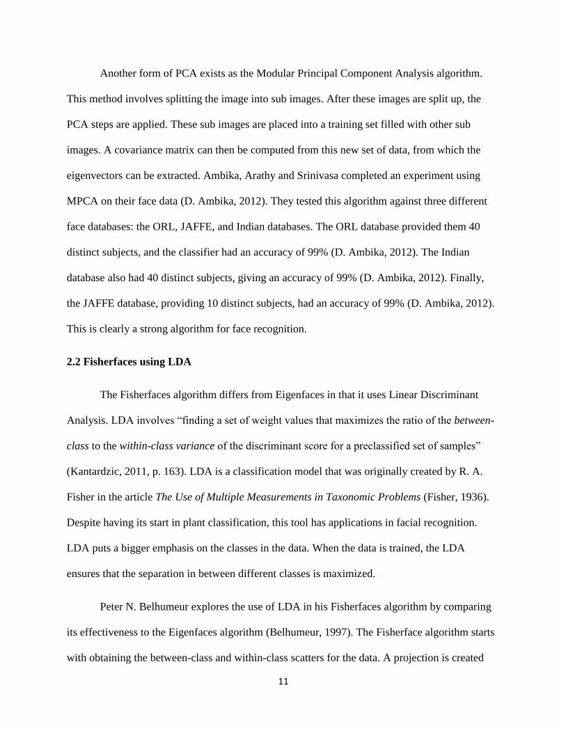
occurred. Figure 12 provides more detail for which faces were unable to be classified properly.
All these images that caused errors, save one, had some sort of shadow effect going on in the
background. It did perform well on faces that had different facial expression. It can be concluded
that this algorithm is too sensitive to the effects of the surroundings and should only be used
when a consistent background can be used.

33
Figure 11: Eigenfaces Confusion Matrix
34
Figure 12: Eigenfaces Errors (Yale Face Database, n.d.)
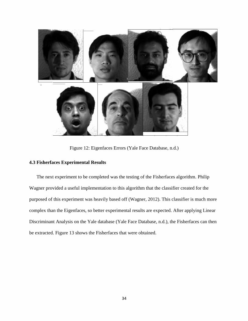
4.3 Fisherfaces Experimental Results
The next experiment to be completed was the testing of the Fisherfaces algorithm. Philip
Wagner provided a useful implementation to this algorithm that the classifier created for the
purposed of this experiment was heavily based off (Wagner, 2012). This classifier is much more
complex than the Eigenfaces, so better experimental results are expected. After applying Linear
Discriminant Analysis on the Yale database (Yale Face Database, n.d.), the Fisherfaces can then
be extracted. Figure 13 shows the Fisherfaces that were obtained.

35
Figure 13: Fisherfaces (Yale Face Database, n.d.)
After employing these Fisherfaces an accuracy of 92% was obtained, as can be seen in table
1. Figure 14 shows the confusion matrix obtained from the Fisherfaces algorithm. Out of the 43
samples in the testing set there were only 3 errors. This is a major improvement over the
Eigenfaces result. Figure 15 shows the errors that resulted from the use of this classifier. Two
faces make a reappearance from the Eigenfaces error list. It appears that the background shadows
can still cause issues within this face recognition classifier; however, it doesn’t have as big hold
as it did in the previous algorithm. Interestingly, two of the faces on the error list have a non-
neutral facial expression. A combination of the shadow background and facial expressions may
also sometimes cause a problem; however, most were classified properly. This classifier also
runs very fast on the Yale Face Database image set. It runs just as fast as the Eigenfaces
algorithm, so that leave very little reason to use that classifier.

36
Figure 14: Fisherface Confusion Matrix
Figure 15: Fisherface Errors (Yale Face Database, n.d.)
37
4.4 Local Binary Patterns Histogram Experimental Results
While the Fisherfaces result was very good, the next experiment will hopefully provide a
better accuracy. The Local Binary Patterns Histogram is the next classifier that is implemented.
The methodology described for this algorithm may seem a little bit complicated at first glance;
however, implementing isn’t overly complicated. In table 1 we can see that using this classifier
on the data from the Yale Face Database provides a 92% accuracy. This provides the same result
as the Fisherfaces classifier. Figure 16 shows the confusion matrix obtained from this classifier.
While it provided the same accuracy as the Fisherfaces algorithm, it has obtained errors on
mostly different images. As can be seen from the LBPH errors in Figure 17, once again the
shadows in the background are causing the occasional error. Interestingly the closed eyes image
was misclassified by all three of the previous algorithms. During the training phase, this
algorithm runs extremely slow. It takes more a minute to train this algorithm, compared the
Fisherfaces which trains in about a second. Testing the algorithm on the Yale Database takes
almost 5 minutes to complete. While taking a long time to run it provides about the same
accuracy as the Fisherfaces algorithm.

38
Figure 16: LBPH Confusion Matrix
Figure 17: LBPH Errors (Yale Face Database, n.d.)

39
4.5 EFL Hybrid Algorithm Experimental Results
Table 2: EFL Hybrid Algorithms Accuracy Based on Highest Rank
Ranked Eigenfaces Ranked Fisherfaces Ranked Local Binary Patterns Histograms
0.92 0.92 0.95
The final algorithm to be implemented is the EFL Hybrid classifier. As was stated
previously, there are three methods for creating this algorithm. Because a voting system is being
used, there is a chance that all three algorithms vote for a different class, which would lead to a
three-way tie. Each algorithm is given a rank so that in the case of a tie, the highest ranked
algorithm’s vote would be declared the winner. Our last experiment will be an implementation of
three possible algorithms with a different classifier as the highest ranked. The experimental
results obtained from using the different variations of the EFL classifier on the Yale Face
Database are displayed in table 2. The algorithm that ranked the Eigenfaces vote as the most
important yielded an accuracy of 92%. While this is a big improvement over the Eigenfaces’
results, it still provides the same results as both the Fisherfaces and the LBPH classifiers. This
algorithm wouldn’t be worth using because it takes more processing time for similar results. The
EFL algorithm which ranked the Fisherfaces vote as the highest provided the same accuracy of
92%. For the same reasoning stated previously, this is obviously not a useful classifier. The final
algorithm is the LBPH ranked classifier. This classifier provides an accuracy of 95%. The EFL
algorithm that ranks LBPH the highest provides the best accuracy. Figure 18 shows the
confusion matrix for this algorithm. If compared with Figure 16, it looks very similar.
Employing the Eigenfaces and Fisherfaces algorithms managed to cut out one of the errors that
previously existed in the LBPH classifier. Figure 19 shows the comparison of the accuracies of

40
each algorithm. The EFL algorithm provides an accuracy that is slightly greater than the
accuracy all its components; however, this boost in accuracy comes at the expense of higher
computational time.
Figure 18: EFL Hybrid Algorithm using LBPH rank Confusion Matrix

41
Figure 19: Comparison of Algorithms
Table 3 displays the run time for each algorithm. In all cases barring the Eigenfaces, the
testing phase appears to take longer than the training phase. Both the Eigenfaces and the
Fisherfaces algorithms run almost instantaneously, whereas the LBPH and the EFL Hybrid
algorithms are much slower. The cost of obtaining a higher accuracy from the EFL Hybrid is the
longer run times.
Table 3: Algorithm Speed (seconds)
Eigenfaces Fisherfaces Local Binary Patterns Histograms EFL Hybrid
Training Phase 1.16 1.89 112.36 115.41
Testing Phase 0.35 2.06 280.38 282.79
0.83
0.92 0.920.95
0.76
0.78
0.8
0.82
0.84
0.86
0.88
0.9
0.92
0.94
0.96
Eigenfaces Fisherfaces Local BinaryPatterns Histograms
EFL Hybrid
Acc
ura
cy
Algorithm
Face Recognition Algorithms

42
CHAPTER V: CONCLUSIONS
5.1 Summary
There were three initial goals stated at the beginning of this thesis. Implementing three
popular face recognition algorithms. Eigenfaces, Fisherfaces and Local Binary Patterns
Histograms were the three algorithms that were implemented. Once these algorithms were
completed, they were run on data obtained from the Yale Face Database (Yale Face Database,
n.d.). The experimental results found that the Eigenface algorithm is significantly worse than
both the Fisherface and the Local Binary Patterns Histograms. All the algorithms discussed were
sensitive to shadows in the background. A consistent background may be necessary for optimal
results. Both the Eigenfaces and the Fisherfaces algorithms run quite a bit faster than the Local
Binary Patterns Histograms algorithm. Due to this fact, the Fisherfaces algorithm should be
considered the best algorithm for this data set. The last goal was to combine these classifiers
such that there is improvement over the originals. When ranking the different algorithms within
the EFL hybrid classifier, both the Eigenfaces and Fisherfaces ranked algorithms didn’t provide
the experimental results that would warrant their usage. On the other hand, the LBPH ranked
classifier provided a slight improvement over its’ opponents. The EFL Hybrid classifier provides
a small increase in accuracy for a bit longer loading time. As technology continues to grow and
improve, the loading times will decrease but the accuracy will remain the same. Face recognition
and machine learning are valuable tools in today’s world, so having access to these algorithms
can be very useful.

43
5.2 Future Work
There are several ways we can improve with future work. Much of the errors that occurred
utilizing these algorithms were caused by shadows in the background of the image. If the images
are properly cropped such that the backgrounds become irrelevant, this may lead to better
experimental results. In this thesis, only three algorithms were combined. Adding even more
algorithms can be an option. The issue with combining more algorithms is the fact that it would
increase the amount of processing time required. This may become more feasible as computer
technology continues to be improved. An interesting concept would be comparing how much
increased accuracy can be obtained at the expense of processing time. This thesis used a method
of combining algorithms by taking the majority result from the classifiers. In future work, a
algorithm can be created that takes the strengths of each of the separate components. Testing
more face databases can also be explored in the future.

44
REFERENCES
Ahonen, T., Hadid, A., & Pietikäinen, M. (2006). Face Description with Local Binary Patterns:
Application to Face Recognition. IEEE Transactions on Pattern Analysis and Machine
Intelligence, 28, 2037-2041.
Anaconda. (2018, November 10). What is Anaconda? Retrieved from
https://www.anaconda.com/what-is-anaconda/
Anggo, M., & Arapu, L. (2018). Face Recognition Using Fisherface Method. Journal of Physics:
Conference Series,1028, 012119. doi:10.1088/1742-6596/1028/1/012119
Bicego, M., Lagorio, A., Grosso, E., & Tistarelli, M. (2006). On the Use of SIFT Features for Face
Authentication. 2006 Conference on Computer Vision and Pattern Recognition Workshop
(CVPRW'06), 35-35.
Bradski, G., & Kaehler, A. (2015). Learning OpenCV. OReilly Media.
Belhumeur, P.N., Hespanha, J.P., & Kriegman, D.J. (1997). Eigenfaces vs. Fisherfaces: Recognition
Using Class Specific Linear Projection. IEEE Trans. Pattern Anal. Mach. Intell., 19, 711-720.
Chan, T. F. (2018, March 16). 7-Eleven is bringing facial-recognition technology pioneered in
China to its 11,000 stores in Thailand. Retrieved from https://www.businessinsider.com/7-
eleven-facial-recognition-technology-introduced-in-thailand-2018-3
Coffin, J. S., & Ingram, D. (1999). U.S. Patent No. 5991429. Washington, DC: U.S. Patent and
Trademark Office.

45
D, Ambika & B. Arathy. B, Arathy & Ramalingam, Srinivasa Perumal. (2012). Comparison of PCA
and MPCA with Different Databases for Face Recognition. International Journal of Computer
Applications. 43. 30-34. 10.5120/6198-8730.
Du, G., Su, F., & Cai, A. (2009). Face recognition using SURF features.
Fisher, R. A. (1936). The Use Of Multiple Measurements In Taxonomic Problems. Annals of
Eugenics,7(2), 179-188. doi:10.1111/j.1469-1809.1936.tb02137.x
Hunter, J., & Dale, D. (2007, May 27). The Matplotlib User’s Guide. Retrieved from
https://social.stoa.usp.br/articles/0015/3893/matplotlib.pdf
Jafri, R., Ali, S.A., & Arabnia, H.R. (2013). Face Recognition for the Visually Impaired.
Jha, A. (2018). Class Room Attendance System Using Facial Recognition System. The International
Journal of Mathematics, Science, Technology and Management,2(3).
Kantardzic, M. (2011). Data mining: concepts, models, methods and algorithms. Oxford: Wiley-
Blackwell.
Kruszka, P., Addissie, Y. A., McGinn, D. E., Porras, A. R., Biggs, E., Share, M., Crowley, T. B.,
Chung, B. H., Mok, G. T., Mak, C. C., Muthukumarasamy, P., Thong, M. K., Sirisena, N. D.,
Dissanayake, V. H., Paththinige, C. S., Prabodha, L. B., Mishra, R., Shotelersuk, V., Ekure, E.
N., Sokunbi, O. J., Kalu, N., Ferreira, C. R., Duncan, J. M., Patil, S. J., Jones, K. L., Kaplan, J.
D., Abdul-Rahman, O. A., Uwineza, A., Mutesa, L., Moresco, A., Obregon, M. G., Richieri-
Costa, A., Gil-da-Silva-Lopes, V. L., Adeyemo, A. A., Summar, M., Zackai, E. H., McDonald-
McGinn, D. M., Linguraru, M. G., … Muenke, M. (2017). 22q11.2 deletion syndrome in diverse
populations. American journal of medical genetics. Part A, 173(4), 879-888.

46
Lee, J. (2017, May 19). Australian passport authority developing facial recognition system.
Retrieved from https://www.biometricupdate.com/201705/australian-passport-authority-
developing-facial-recognition-system
Rahim, A., Md, Hossain, N., Md, Wahid, T., & Azam, S., Md. (2013). Face Recognition using
Local Binary Patterns (LBP). Global Journal of Computer Science and Technology Graphics &
Vision,13(4).
Rahman, M.U. (2012). A comparative study on face recognition techniques and neural
network. CoRR, abs/1210.1916.
Schroeder, C. C. (1998). U.S. Patent No. 5787186. Washington, DC: U.S. Patent and Trademark
Office.
Turk, M., & Pentland, A. (1991). Eigenfaces for Recognition. Journal of Cognitive
Neuroscience,3(1), 71-86. doi:10.1162/jocn.1991.3.1.71
Wagner, P. (2012, July 18). Face Recognition with Python. Retrieved from
https://bytefish.de/pdf/facerec_python.pdf
Walt, S. V., Colbert, S. C., & Varoquaux, G. (2011). The NumPy Array: A Structure for Efficient
Numerical Computation. Computing in Science & Engineering,13(2), 22-30.
doi:10.1109/mcse.2011.37
Wiskott, L., Fellous, J., Krüger, N., & Malsburg, C. V. (1997). Face recognition by elastic bunch
graph matching. Computer Analysis of Images and Patterns Lecture Notes in Computer
Science,456-463. doi:10.1007/3-540-63460-6_150

47
Wiskott, L., Würtz, R. P., & Westphal, G. (2014). Elastic Bunch Graph Matching. Retrieved from
http://www.scholarpedia.org/article/Elastic_Bunch_Graph_Matching
Wold, S., Esbensen, K., & Geladi, P. (1987). Principal Component Analysis. Chemometrics and
Intelligent Laboratory Systems.
Yale Face Database. (n.d.). Retrieved from http://vision.ucsd.edu/content/yale-face-database
Zhao, W., Krishnaswamy, A., Chellappa, R., Swets, D. L., & Weng, J. (1998). Discriminant
Analysis of Principal Components for Face Recognition. Face Recognition,73-85.
doi:10.1007/978-3-642-72201-1_4
Zhang, W., Shan, S., Gao, W., Chen, X., & Zhang, H. (2005). Local Gabor binary pattern histogram
sequence (LGBPHS): a novel non-statistical model for face representation and recognition. Tenth
IEEE International Conference on Computer Vision (ICCV'05) Volume 1, 1, 786-791 Vol. 1.

48
APPENDIX
Appendix A: Face Recognition Parent Class (Part 1)

49
Appendix B: Face Recognition Parent Class (Part 2)

50
Appendix C: Eigenfaces (Part 1)

51
Appendix D: Eigenfaces (Part 2)

52
Appendix E: Fisherfaces (Part 1)

53
Appendix F: Fisherfaces (Part 2)

54
Appendix G: Fisherfaces (Part 3)

55
Appendix H: Local Binary Patterns Histograms (Part 1)

56
Appendix I: Local Binary Patterns Histograms (Part 2)

57
Appendix J: Local Binary Patterns Histograms (Part 3)

58
Appendix K: Local Binary Patterns Histograms (Part 4)

59
Appendix L: EFL Hybrid Algorithm


![Facial Expression Recognition using Hybrid Transform · understanding [1],, psychological studies, facial nerve grading in medicine, face image compression and synthetic face animation](https://img.pdfslide.us/doc/110x75/5f59383509f25316f3204a80/facial-expression-recognition-using-hybrid-transform-understanding-1-psychological.jpg)