Design and Flight Performance of the Orion Pre … · Design and Flight Performance of the Orion Pre-Launch Navigation System Renato Zanetti ... which is a pseudo-measurement consisting

Design and Flight Performance of the Orion

Pre-Launch Navigation System

Renato Zanetti∗

NASA Johnson Space Center, Houston, Texas, 77058, USA

Launched in December 2014 atop a Delta IV Heavy from the Kennedy Space Center,the Orion vehicle’s Exploration Flight Test-1 (EFT-1) successfully completed the objectiveto test the prelaunch and entry components of the system. Orion’s pre-launch absolutenavigation design is presented, together with its EFT-1 performance.

I. Introduction

The Orion capsule, the successor of the Space Shuttle as NASA’s flagship human transportation vehicle,is designed to take men back to the Moon and beyond. The first Exploration Mission (EM1) is scheduled for2018, while its first flight test, EFT-1 (Exploration Flight Test-1), was successfully completed on December5th, 2014. The main objective of the test was to demonstrate the capability to re-enter the Earth’s atmo-sphere and achieve safe splash-down into the Pacific Ocean. This un-crewed mission completes two orbitsaround Earth, the second of which was highly elliptical with an apogee of approximately 5908 km, higherthan any vehicle designed for humans since the Apollo program. The trajectory was designed in order to testa high-energy re-entry similar to those crews will undergo during lunar missions. In order to have a goodnavigation solution during entry, the navigation system operated during pre-flight operations, and duringthe entire flight, even when Orion was not controlling itself but under the control of the launch vehicle orthe upper stage.

Reference ? describes the navigation design of Orion’s EFT-1 mission and the flight performance forthe post-lift phase. The objectives of this paper are to: i. introduce the pad align algorithm design ofthe Orion vehicle, both the Exploration Flight Test 1 design and the changes made in preparation forExploration Missions 1 and 2, and ii. document the performance of the pre-launch navigation system duringEFT-1, which relies on the classic extended Kalman filter (EKF).2 Reference 3 introduced the preliminaryEFT-1 navigation design, while pre-mission simulation performance was shown in reference. 4. The UDUfactorization as introduced by Bierman is employed in the filter design,5 and measurements are included asscalars employing the Carlson6 and Agee-Turner7 Rank-One updates. The possibility of considering onlysome of the filter’s states (rather than estimating all of them8) is included in the design.9

Prior to launch the extended Kalman filter is initialized with the estimated vehicle’s attitude from gyrocompassing (coarse align algorithm) and an inertial position derived from the current time and the coordi-nates of the pad. This pre-launch navigation phase is called fine align and the only measurement active inthis mode during EFT-1 was integrated velocity, which is a pseudo-measurement consisting of a zero changeof Earth-referenced position over a 1 second interval. The GPS receiver measurement are not availableduring fine align because the vehicle, including the GPS antennas, are covered by the launch abort fairing.The main purpose of fine align is to better estimate the attitude and the IMU error states.

II. Inertial Measurement Unit

II.A. The Gyro Model

The gyro is modeled in terms of the bias, scale factor, and non-orthogonality. The IMU case frame isdefined such that the x-axis of the gyro is the reference direction with the x − y plane being the reference

∗GN&C Autonomous Flight Systems Engineer, Aeroscience and Flight Mechanics Division, EG6, 2101 NASA Parkway.AIAA Associate Fellow.

1 of 16

American Institute of Aeronautics and Astronautics

https://ntrs.nasa.gov/search.jsp?R=20160010463 2018-08-20T11:36:48+00:00Z

plane; the y- and z-axes are not mounted perfectly orthogonal to it (this is why we don’t have a fullmisalignment/nonorthogonality matrix as we will in the accelerometer model). The errors in determiningthese misalignments are the so-called non-orthogonality errors, expressed as a matrix Γ, as

Γg =

0 γg3 γg2γg3 0 γg1γg2 γg1 0

The gyro scale factor represents the error in conversion from raw sensor outputs (gyro digitizer pulses) touseful units. In general we model the scale-factor error as a first-order Markov (or a Gauss-Markov) processin terms of a diagonal matrix given as

Sg =

sgx 0 0

0 sgy 0

0 0 sgz

Similarly, the gyro bias errors are modeled as as first-order vector Gauss-Markov processes as

bg =

bgxbgybgz

Finally, the gyro noise is represented by εg. Hence the model of the gyro measurement is given by

ωcm = (I3 + Γg + ∆g) (ωc + bg + εg) = (I3 + ∆g) (ωc + bg + εg) (1)

where I3 is a 3 × 3 identity matrix, the superscript c indicates that this is an inertial measurement at the‘box-level’ expressed in case-frame co-ordinates, and ωc is the ‘true’ angular velocity in the case frame.Notice that since (I + ∆g)−1 ≈ I−∆g, we can express the actual angular velocity in terms of the measuredangular velocity as

ωc = (I3 −∆g)ωcm − bg − εg (2)

The actual measurement provided by gyros is the the accumulated angle:(∆θckck−1

)m

=

∫ tk

tk−1

ωcm(τ) +1

2φccref × ω

cm(τ) dτ (3)

=

∫ tk

tk−1

ωcm(τ) +1

2

[∫ τ

tk−1

φc

cref(χ) dχ

]× ωcm(τ) dτ (4)

=

∫ tk

tk−1

ωcm(τ) +1

2

[∫ τ

tk−1

(ωcm(χ) +

1

2φccref × ω

cm(χ)

)dχ

]× ωcm(τ) dτ

Ignoring second-order terms, we get(∆θckck−1

)m

=

∫ tk

tk−1

[ωcm(τ) +

1

2

∫ τ

tk−1

ωcm(χ) dχ× ωcm(τ)

]dτ (5)

II.B. The Accelerometer Model

Similar to the gyros, the accelerometer scale factor represents the error in conversion from raw sensor outputs(accelerometer digitizer pulses) to useful units. In general we model the scale-factor error as a first-order(Gauss-) Markov process in terms of a diagonal matrix given as

Sa =

sax 0 0

0 say 0

0 0 saz

2 of 16


Similarly, the bias errors are modeled as as first-order Gauss-Markov processes as

ba =

baxbaybaz

So, the accelerometer measurements, acm are modeled as:

acm = (I3 + Sa) (ac + ba + υa) (6)

where I3 is a 3 × 3 identity matrix, the superscript c indicates that this is an inertial measurement at the‘box-level’ expressed in case-frame co-ordinates, and ac is the ‘true’ non-gravitational acceleration in thecase frame. The quantity υa is the velocity random walk, a zero-mean white sequence on acceleration thatintegrates into a velocity random walk, which is the ‘noise’ on the accelerometer output. We note that themeasured ∆v in the case frame, ∆vcm, is mapped to the end of it’s corresponding time interval by the scullingalgorithm within the IMU firmware, so that we can write

(∆vcm)k =

∫ tk

tk−1

Tckc(t)a

c(t)m dt (7)

where (∆vcm)k covers the time interval from tk−1 to tk (tk > tk−1) and c(t) is the instantaneous case framea.We recall that a transformation matrix can be written in terms of the Euler axis/angle as

T (φ) = cos(φ)I − sinφ

φ[φ×] +

1− cosφ

φ2φφT (10)

= I − sinφ

φ[φ×] +

1− cosφ

φ2[φ×] [φ×] (11)

which, for φ ∼ 0 can be approximated as

T (φ) = I − [φ×] (12)

With this in mind, Tckc(t) = I3 −

[θckc(t)×

], and using Eq. (6),

(∆vBm

)k

becomes

(∆vcm)k =

∫ tk

tk−1

[I3 −

[θckc(t)×

]][(I3 + ∆a)ac + ba + υa] dt (13)

We can expand this equation, neglecting terms of second-order, as follows

(∆vcm)k =

∫ tk

tk−1

[I3 −

[θckc(t)×

]]acdt+

∫ tk

tk−1

(ba + υa) dt

+

∫ tk

tk−1

∆aacdt (14)

The first term in the above equation (Eq. (14)) becomes∫ tk

tk−1

[I3 −

[θckc(t)×

]]acdt = (∆vc)k (15)

aOr equivalently, (∆vB

m

)k

=

∫ tk

tk−1

TBkB(t)

aB(t)m dt (8)

But since TBkB(t)

≈ I3 −[φ

BkB(t)

×], we find

(∆vB

m

)k

=

∫ tk

tk−1

[I3 −

[φ

BkB(t)

×]]

aB(t)m dt (9)

3 of 16


and the third term becomes ∫ tk

tk−1

∆aacdt = ∆a

∫ tk

tk−1

acdt ≈∆a (∆vc)k (16)

Finally, the accelerometer noise, which is zero-mean process with spectral density Sa becomes∫ tk+1

tk

υadt = ua (17)

where ua is a random vector with covariance Sa(tk − tk−1). So, Eq. (14) becomes

(∆vcm)k = [I3 + ∆a] (∆vc)k + ba∆t+ υa∆t (18)

Since we have established that [I3 + ∆a]−1 ≈ [I3 −∆a], and neglecting terms of second-order,

(∆vc)k = [I3 −∆a] (∆vcm)k − ba∆t− υa∆t (19)

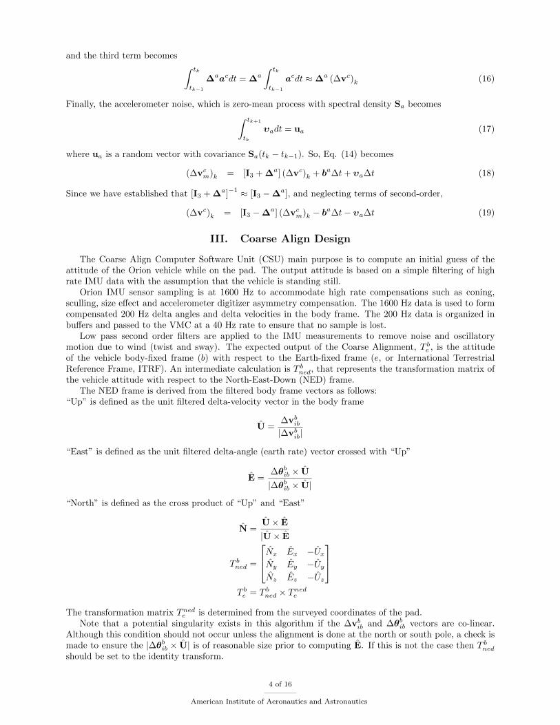
III. Coarse Align Design

The Coarse Align Computer Software Unit (CSU) main purpose is to compute an initial guess of theattitude of the Orion vehicle while on the pad. The output attitude is based on a simple filtering of highrate IMU data with the assumption that the vehicle is standing still.

Orion IMU sensor sampling is at 1600 Hz to accommodate high rate compensations such as coning,sculling, size effect and accelerometer digitizer asymmetry compensation. The 1600 Hz data is used to formcompensated 200 Hz delta angles and delta velocities in the body frame. The 200 Hz data is organized inbuffers and passed to the VMC at a 40 Hz rate to ensure that no sample is lost.

Low pass second order filters are applied to the IMU measurements to remove noise and oscillatorymotion due to wind (twist and sway). The expected output of the Coarse Alignment, T be , is the attitudeof the vehicle body-fixed frame (b) with respect to the Earth-fixed frame (e, or International TerrestrialReference Frame, ITRF). An intermediate calculation is T bned, that represents the transformation matrix ofthe vehicle attitude with respect to the North-East-Down (NED) frame.

The NED frame is derived from the filtered body frame vectors as follows:“Up” is defined as the unit filtered delta-velocity vector in the body frame

U =∆vbib|∆vbib|

“East” is defined as the unit filtered delta-angle (earth rate) vector crossed with “Up”

E =∆θbib × U

|∆θbib × U|

“North” is defined as the cross product of “Up” and “East”

N =U× E

|U× E

T bned =

Nx Ex −UxNy Ey −UyNz Ez −Uz

T be = T bned × Tnede

The transformation matrix Tnede is determined from the surveyed coordinates of the pad.Note that a potential singularity exists in this algorithm if the ∆vbib and ∆θbib vectors are co-linear.

Although this condition should not occur unless the alignment is done at the north or south pole, a check ismade to ensure the |∆θbib × U| is of reasonable size prior to computing E. If this is not the case then T bnedshould be set to the identity transform.

4 of 16


IV. Navigation Algorithm Design

Measurements are incorporated in the navigation solution at 1Hz, which is a typical rate of GPS sensors.However the attitude control algorithm necessitates estimates from the navigation solution at a higher rate,furthermore the IMU measurement data is available at a higher rate. The delta velocity delta attitude accu-mulator (DVDAAccum) CSU is the high-rate Inertial Measurement Unit (IMU) accumulator and attitudepropagator complement to filter CSUs in the 1 Hz rate group. The vehicle attitude is propagated forwardin time through the use of accumulated sensed ∆θ data. The CSU also accumulates ∆V measurementswhich are used by the Position and Velocity Fast Propagator to compute high rate position and velocity fordownstream users. The attitude of DVDAAccum is re-synched to the 1 Hz rate group estimate each second.

DVDAAccum receives feedback data from the 1 Hz EKF CSUs and uses it to perform an update. Duringthe update phase DVDAAccum replaces the estimates of the IMU errors with the most current values,transforms the values of the inertial accumulated delta velocity into the updated inertial frame, and updatesthe inertial to Orion body attitude with the information from the filter.

The Orion fine alignment algorithm utilizes the same Extended Kalman Filter architecture and CSU asthat used for atmospheric navigation (ATMEKF, used during the fine align, ascent, and entry phases). Thispaper presents the design of the fine align portion of the algorithm and trades between three different typeof fine align measurements: Integrated Velocity (IV), Zero Velocity (ZV), and Pad Position (Pos). All thesemeasurements are pseudomeasurents, no sensor exists that produces them, instead the measurements arederived from the fact that the vehicle is not moving with respect to the pad. Hence the actual measurementutilized from the filter is the theoretical value and the measurement noise is given by the variation from thistheoretical value due to twist and sway motion of the stack. This motion is forced by wind and is a functionof the bending modes of the launch system.

During EFT-1, the Orion EKF used an IV measurement, to precisely estimate the attitude of the IMUon the launch pad during the fine align phase. For EM1 and beyond, three possible solutions are considered:

1. The IV measurement returns the change in Earth Centered Earth Fixed (ECEF) position over aspecified amount of time, typically the call rate of the EKF, which for EFT-1 is one second. Thisis a “fake” measurement since no sensor exist and the processed measurement is always given by thenominal value of zero. The measurement noise is therefore given by the true motion of the IMU dueto twist and sway of the stack.

2. The pad position (Pos) measurement returns the planet-fixed position of the IMU. This is also a “fake”measurement always set to the nominal location. The measurement error is comprised not only to thetwist and sway motion, but also of the survey error of the pad location. Therefore the measurementerror has two distinct contributors, a varying component due to the stack oscillations and a repeatablecomponent due to the survey errors.

3. The zero velocity (ZV) measurement returns the instantaneous planet-fixed velocity of the IMU. Thisis also a “fake” measurement always set to the nominal value of zero. The measurement noise is givenby the true motion of the IMU due to twist and sway of the stack.

IV.A. Integrated Velocity

Given the current inertial position ri at time t, the prior inertial position ri0, as well as the transformationmatrix between Earth-fixed and inertial (Ti

e), the IV measurement is given by

yIV = hIV (x,x0, t) =(Tie(t))T

ri −(Tie(t0)

)Tri0 + ηIV = 0 (20)

where hIV (x,x0, t) is the measurement model (note the transpose on the transformation matrix) and ηIVis the measurement noise which exactly cancels out the motion due to twist and sway. The estimatedmeasurement is given by

yIV = hIV (x, x0, t) =(Tie(t))T

ri −(Tie(t0)

)Tri0 (21)

notice that this measurement is nonlinear, potentially highly-nonlinear, since in order to calculate the priorinertial position is necessary to back-integrate the nonlinear equations of motion that also contain the

5 of 16


estimates of the IMU error parameters. Therefore, the measurement residual is

εIV = yIV − yIV (22)

As a first order approximation (used to obtain the IV measurement partials or measurement mapping matrixHIV )

εIV =∂hIV∂x

(x− x) +∂hIV∂x0

(x0 − x0) + ηIV (23)

=∂hIV∂x

x +∂hIV∂x0

Φ(t, t0)x + ηIV (24)

= HIV (x) (x− x) + ηIV (25)

where Φ(t, t0) is the state transition matrix. With this in mind, the partial derivative of the IV measurementis as follows

∂hIV∂r

(x) =(Tie(t))T − (Ti

e(t0))T

Φrr(t, t0) (26)

∂hIV∂v

(x) = −(Tie(t0)

)TΦrv(t, t0) (27)

∂hIV∂φ

(x) = −(Tie(t0)

)TΦrφ(t, t0) (28)

∂hIV∂ba

(x) = −(Tie(t0)

)TΦrba

(t, t0) (29)

∂hIV∂sa

(x) = −(Tie(t0)

)TΦrsa(t, t0) (30)

∂hIV∂ξa

(x) = −(Tie(t0)

)TΦrξa

(t, t0) (31)

∂hIV∂bg

(x) = −(Tie(t0)

)TΦrbg (t, t0) (32)

∂hIV∂sg

(x) = −(Tie(t0)

)TΦrsg (t, t0) (33)

∂hIV∂γg

(x) = −(Tie(t0)

)TΦrγg

(t, t0) (34)

The measurement noise is given by the change in position due to sway over one second. Notice that becauseof the back-propagation, this measurement is nonlinear in nature. Due to the oscillatory motion due to theflex modes of the stack, this nonlinearity could be potentially severe, although severe nonlinearities are notexpected over one second intervals nor were they experience during EFT-1.

IV.B. Pad Position Measurement

The position measurement is expressed as follows:

yPos = hPos(x, t) =(Tie(t))T

ri + bpad + ηPos (35)

where bpad is the launch pad location survey error and ηPos is the measurement noise which exactly cancelsout the motion due to twist and sway. The estimated measurement is given by

yPos = hPos(x, t) =(Tie(t))T

ri + bpad (36)

The measurement residual is

εPos = yPos − yPos = HPos(x) x + ηPos (37)

6 of 16


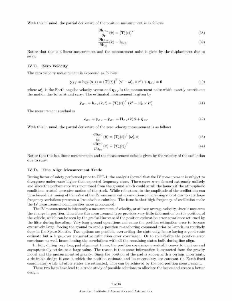
With this in mind, the partial derivative of the position measurement is as follows

∂hPos∂r

(x) =(Tie(t))T

(38)

∂hPos∂bse

(x) = I3×3 (39)

Notice that this is a linear measurement and the measurement noise is given by the displacement due tosway.

IV.C. Zero Velocity

The zero velocity measurement is expressed as follows:

yZV = hZV (x, t) =(Tie(t))T (

vi − ωiE × ri)

+ ηZV = 0 (40)

where ωiE is the Earth angular velocity vector and ηZV is the measurement noise which exactly cancels outthe motion due to twist and sway. The estimated measurement is given by

yZV = hZV (x, t) =(Tie(t))T (

vi − ωiE × ri)

(41)

The measurement residual is

εZV = yZV − yZV = HZV (x) x + ηZV (42)

With this in mind, the partial derivative of the zero velocity measurement is as follows

∂hZV∂r

(x) =(Tie(t))T

[ωiE×] (43)

∂hZV∂bse

(x) =(Tie(t))T

(44)

Notice that this is a linear measurement and the measurement noise is given by the velocity of the oscillationdue to sway.

IV.D. Fine Align Measurement Trade

During factor of safety performed prior to EFT-1, the analysis showed that the IV measurement is subject todivergence under some higher-than-expected frequency cases. These cases were deemed extremely unlikelyand since the performance was monitored from the ground which could scrub the launch if the atmosphericconditions created excessive motion of the stack. While robustness to the amplitude of the oscillations canbe achieved via tuning of the value of the IV measurement noise variance, increasing robustness to very largefrequency variations presents a less obvious solution. The issue is that high frequency of oscillation makethe IV measurement nonlinearities more pronounced.

The IV measurement is inherently a measurement of velocity, or at least average velocity, since it measuresthe change in position. Therefore this measurement type provides very little information on the position ofthe vehicle, which can be seen by the gradual increase of the position estimation error covariance returned bythe filter during fine align. Very long ground operations can cause the position estimation error to becomeexcessively large, forcing the ground to send a position re-anchoring command prior to launch, as routinelydone in the Space Shuttle. Two options are possible, overwriting the state only, hence having a good stateestimate but a large, over conservative estimation error covariance. Or to re-initialize the position errorcovariance as well, hence loosing the correlations with all the remaining states built during fine align.

In fact, during very long pad alignment times, the position covariance eventually ceases to increase andasymptotically settles to a large value. The reason is that some information is extracted from the gravitymodel and the measurement of gravity. Since the position of the pad is known with a certain uncertainty,a desirable design is one in which the position estimate and its uncertainty are constant (in Earth-fixedcoordinates) while all other states are estimated. This can be achieved by the pad position measurement.

These two facts have lead to a trade study of possible solutions to alleviate the issues and create a betterdesign.

7 of 16


The most important aspect of the trade is whether or not a position re-anchoring is necessary. Groundcommands not only increase the complexity of the code, but, more importantly, require controllers to spendconsiderable time developing and studying flight rules to handle various scenarios. A position re-anchoringcan be automatically forced immediately prior to launch, however this has the unwanted side effect of eithera largely conservative position covariance, or cancelling all the correlation between position and other states,which in turn are used to estimate the other states from pseudo range measurements during ascent. The padposition measurement keeps the estimated position error covariance constant during ground align operations,and never necessitates of a re-anchoring. Both IV and ZV measurement have very weak position observability,which comes from either the fact that gravity is a function of position or from ω× r due to Earth’s rotation;goth have a very low sensitivity to position changes.

In all aspects of flight software design, it is also very important to keep the algorithm as simple as possiblewhile meeting requirements. ZV and Pos measurements are both linear, do not require back propagation ofthe state, and hence are significantly simpler to implement than IV. Of the two, ZV is the simpler becauseit does not require the addition of any other state. The need of pad position bias states is imperativein processing pad measurement. The survey error is done only once, therefore processing the measurementevery second results in a constant error, furthermore this survey value is used to initialize the filter, hence theinitial error is correlated to the measurement error. The need for extra states, and hence a larger covariancematrix and more computations, is highly mitigated by the fact that GPSR measurement are not processedwhile on the pad and they also necessitate extra states. Therefore the GPS clock bias and drift states forthe two receivers are recycled as pad position bias states. As a result the pad position measurement doesnot require any increase on the size of the EKF state vector.

While filter divergence is a very serious issue that must be taken into consideration, the situations in whichIV measurement caused divergence of the filter were extreme and deemed very unlikely to occur. Even ifthey did occur, it would probably be due to bad weather and monitored by the ground which would postponethe launch. Therefore divergence issues are the lowest weighted element of the trade. Pad position and ZVare linear measurements, therefore they cannot cause divergence during a measurement update (divergencecan occur during propagation, but that is completely independent from the choice of measurement update).

Given these three aspects of the trade, pad position measurements were deemed the best solution forOrion going forward and replaced IV for Exploration Mission 1 and beyond. Table 1 shows the matrix ofthe trade.

Table 1. Fine Align Measurements Trade Matrix

Trade Factor Trade Weight IV Pos ZV

Avoid position re-anchor High NO YES NO

Lower algorithm complexity Medium NO NO YES

Avoid potential divergence Low NO YES NO

IV.E. Exploration Mission I Design

The Orion atmospheric extended Kalman filter (ATMEKF) processes all available observations each cycle toestimate position, velocity, and alignment, along with the measurement error parameters. All inertial sensorerror estimates are fed back as corrections each cycle during the INS state correction process. The U-D-Ualgorithm is used in the ATMEKF processing to avoid any possible numerical instability.

From the trade study discussed above, the pad position measurement is processed by the filter. Theobservation is based on the fact that, during ground alignment, the navigation base is not moving with respectto Earth, other than twist and sway. The surveyed position of the stack is therefore used as an externalmeasurement and it is compared to the propagated position using gravity and IMU data. This observationcan be mapped directly into the integrated position state via the Earth-Fixed to Inertial transformationmatrix. Two errors affect the measurement. The first is due to oscillations because of twist and sway, thiserror source is aleatory in nature and modeled as white noise. The second source of error is repeatable, andis given by the survey error of the pad location together with the error in establishing the position of theIMUs with respect to the pad. This error is accounted for as a state in the filter.

The normalized squared measurement residuals values for each of the three components of the position

8 of 16


observation are calculated prior to processing any observations. If any of the three values values exceeds thelimit, all observation components are discarded for this cycle.

The state vector components are divided in dynamic-states and parameter-states. Parameter-states differfrom the other states in that they are modeled as first order Markov processes, therefore their time evolutionis known analytically and does not necessitate numerical integration. In addition, their state transitionmatrix is also known analytically and it is very sparse, making their covariance matrix propagation extremelynumerically efficient.

The states are partitioned into vehicle dynamic states, X , and the parameter-states (IMU errors, GPSPR errors), B, so that

X =[X T BT

]T(45)

We explicitly include the attitude as a state in order to properly model the coupling inherent in a strap-down IMU (particularly during accelerated flight). As stated earlier the parameter-states are modeled asfirst-order Gauss-Markov processes and use a much more efficient computational algorithm for the updateof the covariance matrix. Tables 2 and 3 list the states and parameters within the Atmospheric EKF.

Table 2. Atmospheric Navigation States

State Number of Description

elements

Position 3 Position vector in inertial coordinates

Velocity 3 Velocity vector in inertial coordinate

Attitude 3 Multiplicative attitude deviation state

Clock Bias and Drift 4 One pair per receiver, three of these states are used as

pad position bias states during fine align

Table 3. Atmospheric Navigation Parameters

Parameter Number of

elements

gyro bias 3

gyro scale factor 3

accel bias 3

accel scale factor 3

pseudorange bias 12

Position, velocity, and attitude states and their covariance are initialized as appropriate directly fromdata provided to the CSU. During Pad initialization scenarios, states 10 to 12 are initialized as pad biasstates. The pad position measurement is expressed in the ITRF and is modeled as

ypad = re + bepad + ηpad

where re is the ITRF position vector, bepad is the survey error of the pad position, and ηpad is the non-repeatable error of the measurement (e.g. due to twist and sway motion). The filter is initialized with thepad surveyed position coordinated in the inertial frame, that is, the initial position estimate is given by

r(t0) = Tie(t0) ypad

where Tie is the DCM transforming inertial coordinates into ICRF coordinates, therefore the initial position

estimation error er(t0) is given by

er(t0) = r(t0)− r(t0) = Tie(t0)re −Ti

e(t0)(re + bepad + ηpad) (46)

= −Tie(t0)bepad −Ti

e(t0)ηpad = −Tie(t0)eebpad

−Tie(t0)ηpad (47)

9 of 16


The last equality holds because the initial estimated pad survey error is zero (otherwise the estimate errorwould be subtracted from the estimated position resulting in a new estimated position with zero estimatederror). Equation (47) shows the correlation between the initial position and the survey error state, from itwe deduce the values for the following elements of the initial covariance matrix

P0(bpad, bpad) = Tei (t0) P0(r, r) Ti

e(t0) (48)

P0(X, bpad) = P0(X, r) Tie(t0) (49)

P0(bpad, X) = Tei (t0) P0(r,X) (50)

where P0(bpad, bpad) is the 3×3 covariance of the pad survey error state, P0(r, r) is the 3×3 initial covarianceof the position state, P0(X, bpad) is the cross covariance between any state X and the pad survey errorstate. The resulting 12x12 position, velocity, attitude, and pad survey error covariance matrix is generallynon-diagonal and is converted to its UDU factorization for the filter to use. During non-pad initializationcases, states 10 to 12 are left unitialized; they will be initialized, together with state 13, once valid GPSmeasurements are received by the filter.

V. Pre-Launch EFT-1 Performance

Process noise is used to tune the filter. For the Orion Absolute Navigation Filter, the process noise entersthe covariance update via the dynamic states and the parameter states. For the position and velocity, theprocess noise enters via the velocity state; the process noise represents the uncertainty in the dynamics,chiefly caused by mis-modeled (or unmodeled) accelerations. Since the accelerometers only measure non-inertial forces, gravity is modeled via a high-order gravity model. For the Orion Absolute Navigation filter,Earth’s gravity is modeled by an 8 × 8 gravity field; higher-order spherical harmonics are neglected andhence are captured by the velocity process noise. Additionally, since the attitude rate states are not partof the filter, the attitude process noise enters via the gyro angle random walk. The velocity and attitudeprocess noises are obtained from the IMU Velocity Random Walk and Angular Random Walk performance,respectively. Conservative values of 0.96741 ft2/s and 0.0096741ft2/s3 are used for the clock bias and driftprocess noise, respectively.

The IMU states are modeled as first-order Gauss-Markov processes and carry with them correspondingprocess noise parameters which are used in the tuning of the filter. Since the IMU errors were expected tobe quite constant during the 4.5 hour flight, the time constant of these parameters was chosen as 4 hours,and the process noise was chosen such that the steady-state value of the Markov processes was equal to thevendor’s specification.

During fine align the navigation filter process integrated velocity (IV) measurements. Figure 1 showsthe performance of the filter processing this measurement by means of the measurement residual (actualmeasurement minus estimated measurement, blue lines) and their predicted covariance (red lines). It can beseen that the residuals are well within their predicted variance, all of the measurements are accepted (greenline) and zero rejections occur (red line). The residuals are extremely small with respect to their predictedstandard deviation, this suggests the filter is overly conservative. This fact was expected and a design choiceto add robustness to large twist and sway motion of the launch vehicle. During the day of flight little to notwist and sway was observed. Figure 1 shows the results from Channel 1. A zoomed in plot of the residualsfrom Channel 2 is shown in Figure 2. Throughout the flight the performance of the two channels is nearlyidentical, therefore only results from Channel 1 are shown for the remainder of this paper.

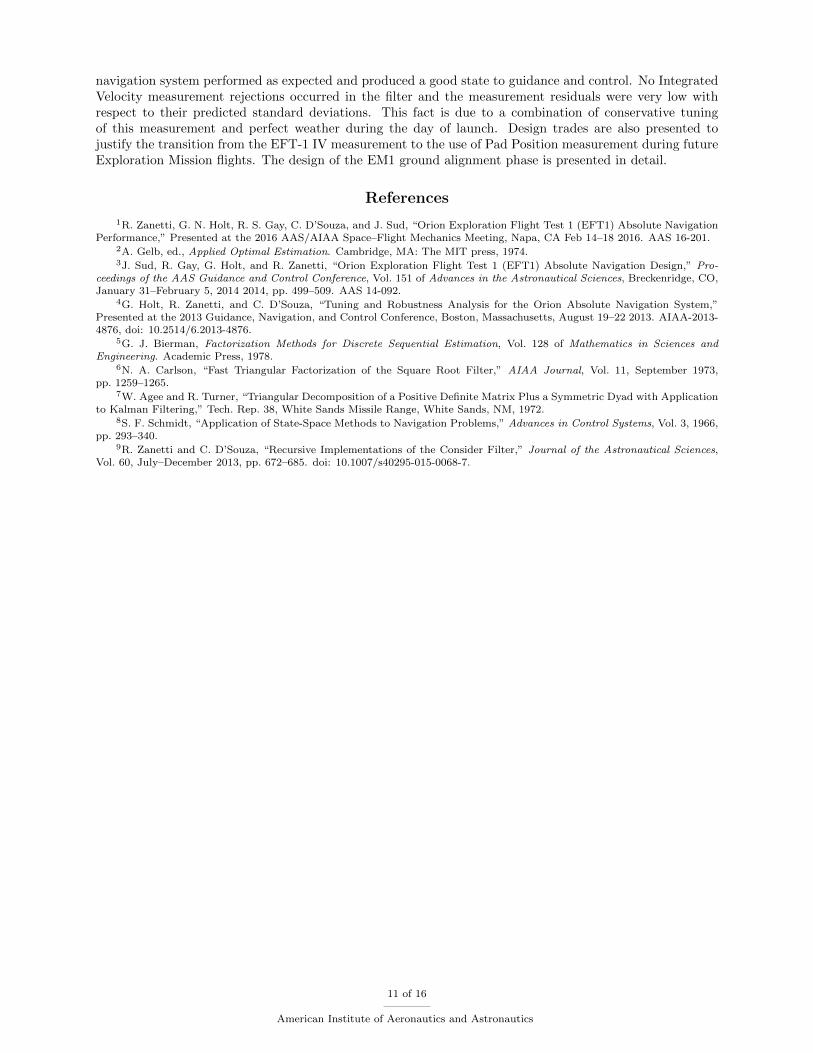
Figure 3 shows the filter’s position, velocity, and attitude covariance. Figures 4 and 5 show the ac-celerometer and gyro error states covariance, respectively. Figures 6 and 7 show the filter’s estimates of theaccelerometer and gyro errors, respectively. The performance is as expected.

Finally, Figures 8 to 10 show the position, velocity, and attitude estimates from the user parametersprocessor (UPP) which provided the outputs from channel 1.

VI. Conclusions

This paper documents the design of the Orion ground navigation system and presents its performanceduring Exploration Flight Test 1 (EFT-1). Characteristics of the EFT-1 design were introduced, and datafrom the flight is shown to validate the design choices. This data illustrates a flight in which the absolute

10 of 16


navigation system performed as expected and produced a good state to guidance and control. No IntegratedVelocity measurement rejections occurred in the filter and the measurement residuals were very low withrespect to their predicted standard deviations. This fact is due to a combination of conservative tuningof this measurement and perfect weather during the day of launch. Design trades are also presented tojustify the transition from the EFT-1 IV measurement to the use of Pad Position measurement during futureExploration Mission flights. The design of the EM1 ground alignment phase is presented in detail.

References

1R. Zanetti, G. N. Holt, R. S. Gay, C. D’Souza, and J. Sud, “Orion Exploration Flight Test 1 (EFT1) Absolute NavigationPerformance,” Presented at the 2016 AAS/AIAA Space–Flight Mechanics Meeting, Napa, CA Feb 14–18 2016. AAS 16-201.

2A. Gelb, ed., Applied Optimal Estimation. Cambridge, MA: The MIT press, 1974.3J. Sud, R. Gay, G. Holt, and R. Zanetti, “Orion Exploration Flight Test 1 (EFT1) Absolute Navigation Design,” Pro-

ceedings of the AAS Guidance and Control Conference, Vol. 151 of Advances in the Astronautical Sciences, Breckenridge, CO,January 31–February 5, 2014 2014, pp. 499–509. AAS 14-092.

4G. Holt, R. Zanetti, and C. D’Souza, “Tuning and Robustness Analysis for the Orion Absolute Navigation System,”Presented at the 2013 Guidance, Navigation, and Control Conference, Boston, Massachusetts, August 19–22 2013. AIAA-2013-4876, doi: 10.2514/6.2013-4876.

5G. J. Bierman, Factorization Methods for Discrete Sequential Estimation, Vol. 128 of Mathematics in Sciences andEngineering. Academic Press, 1978.

6N. A. Carlson, “Fast Triangular Factorization of the Square Root Filter,” AIAA Journal, Vol. 11, September 1973,pp. 1259–1265.

7W. Agee and R. Turner, “Triangular Decomposition of a Positive Definite Matrix Plus a Symmetric Dyad with Applicationto Kalman Filtering,” Tech. Rep. 38, White Sands Missile Range, White Sands, NM, 1972.

8S. F. Schmidt, “Application of State-Space Methods to Navigation Problems,” Advances in Control Systems, Vol. 3, 1966,pp. 293–340.

9R. Zanetti and C. D’Souza, “Recursive Implementations of the Consider Filter,” Journal of the Astronautical Sciences,Vol. 60, July–December 2013, pp. 672–685. doi: 10.1007/s40295-015-0068-7.

11 of 16


Figure 1. FCM1-CH1 IV Measurements

Figure 2. FCM1-CH2 IV Measurements

12 of 16


Figure 3. FCM1-CH1 Position, Velocity, and Attitude 3σ Covariance

Figure 4. FCM1-CH1 Accelerometer Bias, Scale Factor, and Misalignment 3σ Covariance

13 of 16


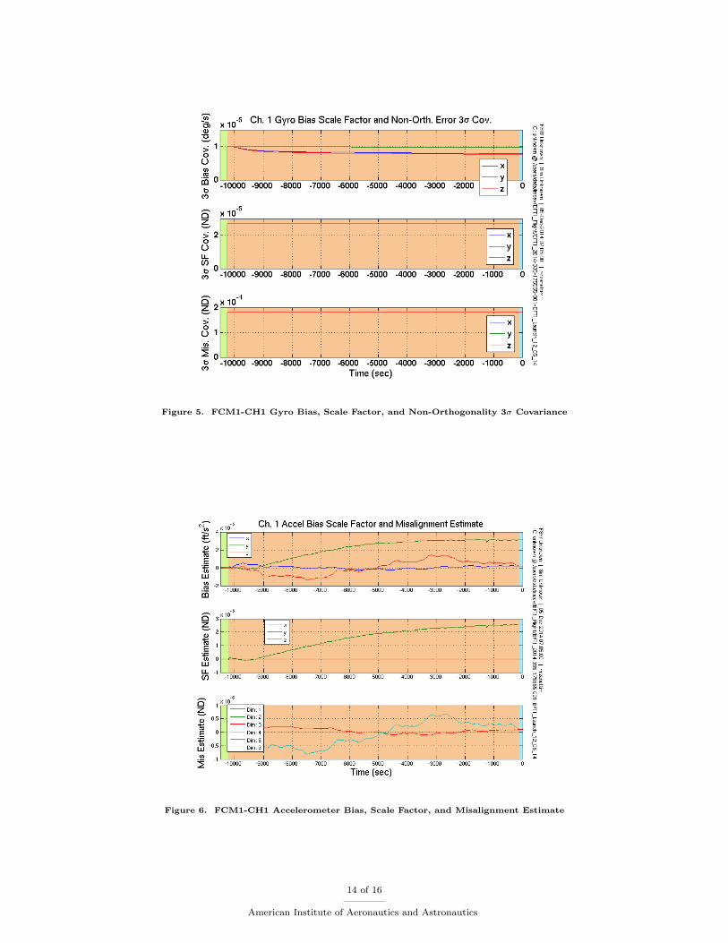
Figure 5. FCM1-CH1 Gyro Bias, Scale Factor, and Non-Orthogonality 3σ Covariance

Figure 6. FCM1-CH1 Accelerometer Bias, Scale Factor, and Misalignment Estimate

14 of 16


Figure 7. FCM1-CH1 Gyro Bias, Scale Factor, and Non-Orthogonality Estimate

Figure 8. FCM1-CH1 Position Estimate

15 of 16


Figure 9. FCM1-CH1 Velocity Estimate

Figure 10. FCM1-CH1 Attitude Estimate

16 of 16


Documents

Design and Flight Performance of the Orion Pre … · Design and Flight Performance of the Orion Pre-Launch Navigation System Renato Zanetti ... which is a pseudo-measurement consisting