Design and Flight-Path Simulation of a Dynamic-Soaring UAV

PhD Dissertations and Master's Theses

Summer 7-2021

Design and Flight-Path Simulation of a Dynamic-Soaring UAV Design and Flight-Path Simulation of a Dynamic-Soaring UAV

Gladston Joseph [email protected]

Follow this and additional works at: https://commons.erau.edu/edt

Part of the Aerodynamics and Fluid Mechanics Commons, Aeronautical Vehicles Commons,

Navigation, Guidance, Control and Dynamics Commons, Other Aerospace Engineering Commons, and the

Propulsion and Power Commons

Scholarly Commons Citation Scholarly Commons Citation Joseph, Gladston, "Design and Flight-Path Simulation of a Dynamic-Soaring UAV" (2021). PhD Dissertations and Master's Theses. 599. https://commons.erau.edu/edt/599

This Thesis - Open Access is brought to you for free and open access by Scholarly Commons. It has been accepted for inclusion in PhD Dissertations and Master's Theses by an authorized administrator of Scholarly Commons. For more information, please contact [email protected].

http://commons.erau.edu/

http://commons.erau.edu/

https://commons.erau.edu/edt

https://commons.erau.edu/edt?utm_source=commons.erau.edu%2Fedt%2F599&utm_medium=PDF&utm_campaign=PDFCoverPages

http://network.bepress.com/hgg/discipline/222?utm_source=commons.erau.edu%2Fedt%2F599&utm_medium=PDF&utm_campaign=PDFCoverPages





https://commons.erau.edu/edt/599?utm_source=commons.erau.edu%2Fedt%2F599&utm_medium=PDF&utm_campaign=PDFCoverPages

mailto:[email protected]

Design and Flight-Path Simulation of a Dynamic-Soaring UAV

By

Gladston Joseph

A Thesis Submitted to the Faculty of Embry-Riddle Aeronautical University

In Partial Fulfillment of the Requirements for the Degree of

Master of Science in Aerospace Engineering

July 2021

Embry-Riddle Aeronautical University

Daytona Beach, Florida

Daewon Kim 8/3/2021

8/3/2021

8/3/2021

iii

ACKNOWLEDGEMENTS

“In the beginning God created the heavens and the earth”

- Genesis 1:1 NKJV

I would like to thank my advisors, Dr. Vladimir Golubev, and Dr. Snorri

Gudmundsson for their expertise, guidance and the moral support.

I would also like to extend my acknowledgement to Dr. William Mackunis and

Dr. Hever Moncayo for their guidance in the development of control laws.

My gratitude goes towards my father, Mr. Stephen Leo and my mother, Dr. Joanofarc

for their prayers and support during this time.

I would also like to acknowledge the mentorship from Dr. Ravi Margasahayam, a

NASA Docent, and a Global Space Ambassador.

Lastly, I would like to express my gratitude to the university for the financial and

technical support that made this work possible.

iv

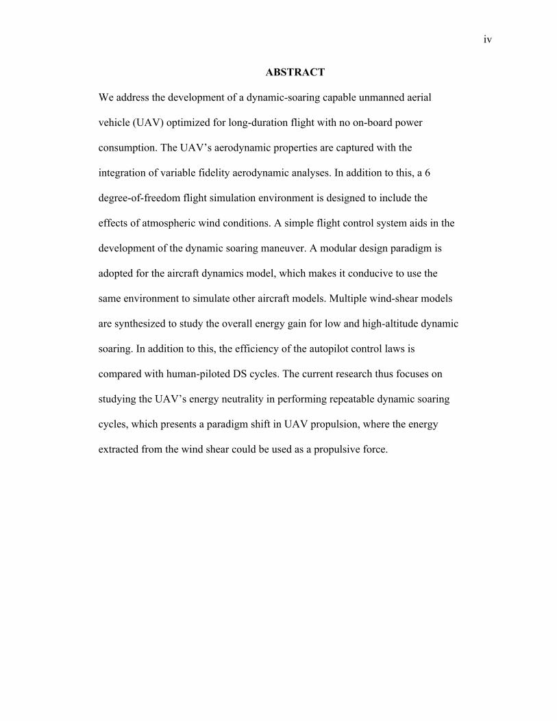
ABSTRACT

We address the development of a dynamic-soaring capable unmanned aerial

vehicle (UAV) optimized for long-duration flight with no on-board power

consumption. The UAV’s aerodynamic properties are captured with the

integration of variable fidelity aerodynamic analyses. In addition to this, a 6

degree-of-freedom flight simulation environment is designed to include the

effects of atmospheric wind conditions. A simple flight control system aids in the

development of the dynamic soaring maneuver. A modular design paradigm is

adopted for the aircraft dynamics model, which makes it conducive to use the

same environment to simulate other aircraft models. Multiple wind-shear models

are synthesized to study the overall energy gain for low and high-altitude dynamic

soaring. In addition to this, the efficiency of the autopilot control laws is

compared with human-piloted DS cycles. The current research thus focuses on

studying the UAV’s energy neutrality in performing repeatable dynamic soaring

cycles, which presents a paradigm shift in UAV propulsion, where the energy

extracted from the wind shear could be used as a propulsive force.

v

TABLE OF CONTENTS

ACKNOWLEDGEMENTS........................................................................................... iii ABSTRACT................................................................................................................... iv LIST OF FIGURES........................................................................................................ vii LIST OF TABLES......................................................................................................... xi NOMENCLATURE....................................................................................................... xii 1. Introduction................................................................................................................ 1

1.1. The Dynamic Soaring Cycles............................................................................ 1 1.2. Using Creation as a Model for Design.............................................................. 2

1.2.1. Termite Inspired Buildings...................................................................... 3 1.2.2. Kingfisher Inspired Bullet Trains............................................................. 4 1.2.3. Woodpecker Inspired Shock Absorbers................................................... 5

1.3. Importance of Research..................................................................................... 5 2. Review of the Relevant Literature............................................................................. 6 3. Methodology.............................................................................................................. 12

3.1. Acquiring the Aerodynamic Model.................................................................. 12 3.1.1. Initial Aircraft Geometry Design............................................................. 13 3.1.2. Integration of Variable Fidelity Analysis................................................ 15

3.1.2.1. SURFACES..................................................................................... 15 3.1.2.2. ANSYS Fluent................................................................................ 15 3.1.2.3. Numerical Implementation.............................................................. 16

3.1.2.3.1. ANSYS Fluent Model............................................................ 16 3.1.2.3.1.1. Model Geometry........................................................... 17 3.1.2.3.1.2. Model Grid Structure.................................................... 18

3.1.2.3.2. SURFACES Model................................................................ 19 3.1.3. Selecting the Turbulence Model.............................................................. 20

3.1.3.1. Methodology to Compare the Turbulence Models......................... 20 3.1.3.1.1. Isolated Wing Simulation....................................................... 20 3.1.3.1.2. CFD Simulations of Complete Aircraft Geometry................ 21

3.1.3.2. Comparison for Selected Stages of DS Flight Path........................ 23 3.1.4. Variations of Aerodynamic Characteristics............................................. 26

3.1.4.1. Angle of Attack Sweep................................................................... 26 3.1.4.2. Yaw Sweep...................................................................................... 29 3.1.4.3. Roll Sweep...................................................................................... 30 3.1.4.4. Dynamic Stability Derivatives........................................................ 30

3.2. Building the Flight Simulation Environment.................................................... 30 3.2.1. Aircraft Dynamics.................................................................................... 31

3.2.1.1. Lookup Tables................................................................................. 33

vi

3.2.1.2. Aerodynamics................................................................................. 35 3.2.1.3. Thrust Model................................................................................... 36 3.2.1.4. Linear Acceleration and Moments.................................................. 37 3.2.1.5. Equations of Motion and Numerical Integration............................ 38 3.2.1.6. Flight Parameters............................................................................ 38

3.2.2. Synthesizing the Wind Model.................................................................. 39 3.2.2.1. Logarithmic Wind Shear................................................................. 40 3.2.2.2. Simple Wind Model........................................................................ 41

3.2.3. Autopilot and Controls............................................................................. 41 3.2.3.1. Waypoint Controller........................................................................ 42 3.2.3.2. Closed Loop Control System.......................................................... 44 3.2.3.3. Flightgear Implementation.............................................................. 47 3.2.3.4. Human-Piloted System.................................................................... 48

3.3. Modifying the Aerodynamic Model.................................................................. 50 4. Results........................................................................................................................ 53

4.1. Auto-Pilot Controlled Dynamic Soaring........................................................... 53 4.1.1. Logarithmic Wind Shear at Maximum Wind Speed = 30 ft/s................. 54 4.1.2. Simple Wind Model at Wind Speed = 30 ft/s.......................................... 55 4.1.3. Total Distance Travelled.......................................................................... 56 4.1.4. Minimum Wind Shear Required.............................................................. 59

4.2. Human-Piloted Dynamic Soaring..................................................................... 60 5. Discussions, Conclusions, and Recommendations.................................................... 64

5.1. Discussions........................................................................................................ 64 5.1.1. Hybrid Aerodynamic Model.................................................................... 64 5.1.2. 6DoF Flight Simulation Environment...................................................... 65

5.2. Conclusions....................................................................................................... 65 5.3. Recommendations............................................................................................. 67

REFERENCES............................................................................................................... 68 APPENDIX A................................................................................................................ 70 APPENDIX B................................................................................................................ 71

vii

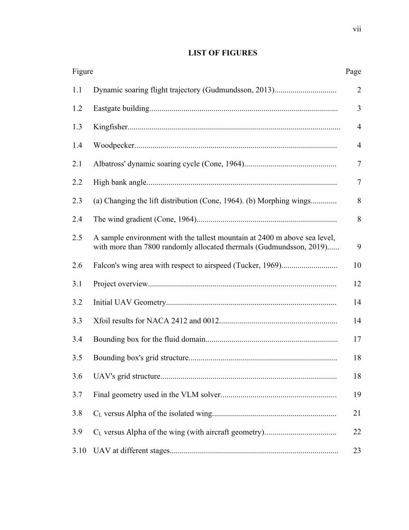
LIST OF FIGURES

Figure Page 1.1 Dynamic soaring flight trajectory (Gudmundsson, 2013)............................... 2 1.2 Eastgate building.............................................................................................. 3 1.3 Kingfisher.......................................................................................................... 4 1.4 Woodpecker..................................................................................................... 4 2.1 Albatross' dynamic soaring cycle (Cone, 1964).............................................. 7 2.2 High bank angle............................................................................................... 7 2.3 (a) Changing the lift distribution (Cone, 1964). (b) Morphing wings............. 8 2.4 The wind gradient (Cone, 1964)...................................................................... 8 2.5 A sample environment with the tallest mountain at 2400 m above sea level,

with more than 7800 randomly allocated thermals (Gudmundsson, 2019)...... -----

9 2.6 Falcon's wing area with respect to airspeed (Tucker, 1969)............................ 10 3.1 Project overview.............................................................................................. 12 3.2 Initial UAV Geometry..................................................................................... 14 3.3 Xfoil results for NACA 2412 and 0012........................................................... 14 3.4 Bounding box for the fluid domain.................................................................. 17 3.5 Bounding box's grid structure.......................................................................... 18 3.6 UAV's grid structure........................................................................................ 18 3.7 Final geometry used in the VLM solver.......................................................... 19 3.8 CL versus Alpha of the isolated wing.............................................................. 21 3.9 CL versus Alpha of the wing (with aircraft geometry).................................... 22 3.10 UAV at different stages.................................................................................... 23

viii

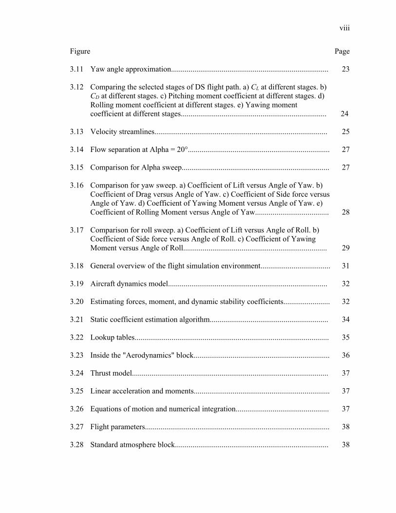
Figure Page 3.11 Yaw angle approximation................................................................................. 23 3.12 Comparing the selected stages of DS flight path. a) CL at different stages. b)

CD at different stages. c) Pitching moment coefficient at different stages. d) Rolling moment coefficient at different stages. e) Yawing moment coefficient at different stages...........................................................................

--------------------24

3.13 Velocity streamlines......................................................................................... 25 3.14 Flow separation at Alpha = 20°......................................................................... 27 3.15 Comparison for Alpha sweep............................................................................ 27 3.16 Comparison for yaw sweep. a) Coefficient of Lift versus Angle of Yaw. b)

Coefficient of Drag versus Angle of Yaw. c) Coefficient of Side force versus Angle of Yaw. d) Coefficient of Yawing Moment versus Angle of Yaw. e) Coefficient of Rolling Moment versus Angle of Yaw......................................

--------------

-----28

3.17 Comparison for roll sweep. a) Coefficient of Lift versus Angle of Roll. b)

Coefficient of Side force versus Angle of Roll. c) Coefficient of Yawing Moment versus Angle of Roll..........................................................................

------------

29 3.18 General overview of the flight simulation environment.................................... 31 3.19 Aircraft dynamics model.................................................................................. 32 3.20 Estimating forces, moment, and dynamic stability coefficients........................ 32 3.21 Static coefficient estimation algorithm............................................................. 34 3.22 Lookup tables.................................................................................................... 35 3.23 Inside the "Aerodynamics" block...................................................................... 36 3.24 Thrust model..................................................................................................... 37 3.25 Linear acceleration and moments...................................................................... 37 3.26 Equations of motion and numerical integration................................................ 37 3.27 Flight parameters............................................................................................... 38 3.28 Standard atmosphere block............................................................................... 38

ix

Figure Page 3.29 Synthesizing the wind model............................................................................ 39 3.30 Wind forces connected to force equations & flat earth navigation................... 40 3.31 Visual representation of the wind models......................................................... 41 3.32 Autopilot system design.................................................................................... 42 3.33 Waypoint controller.......................................................................................... 43 3.34 Waypoint counter.............................................................................................. 43 3.35 Rate of climb calculator.................................................................................... 44 3.36 Visual representation of PID equations............................................................. 45 3.37 Inner and outer loops for directional control..................................................... 45 3.38 Rate saturators................................................................................................... 45 3.39 Flightgear visualization..................................................................................... 47 3.40 Switching from flat earth to LLA coordinate system........................................ 48 3.41 Simulink to Flightgear interface........................................................................ 48 3.42 Joystick null-zones and sensitivity.................................................................... 49 3.43 SURFACES model of the “Albatross” UAV.................................................... 51 3.44 Lift to drag ratio of the "Albatross" UAV......................................................... 52 4.1 a) Speed & Altitude versus Time for Logarithmic wind shear with max wind

speed = 30 ft/s, b) Energy versus Time for logarithmic wind shear with max wind speed = 30 ft/s...........................................................................................

------------

55 4.2 a) Speed & Altitude versus Time for simple wind model with max wind

speed = 30 ft/s, b) Energy versus Time for simple wind model with max wind speed = 30 ft/s...........................................................................................

------------

57 4.3 Auto-piloted dynamic soaring flight path......................................................... 58 4.4 Auto-piloted dynamic soaring flight path (First three cycles).......................... 58

x

Figure Page 4.5 Total distance travelled by the auto-piloted UAV in approximately 20

dynamic soaring cycles..................................................................................... -----

59 4.6 Speed & Altitude versus Time for Logarithmic wind shear with max wind

speed = 27 ft/s.................................................................................................... -----

60 4.7 a) Speed & Altitude versus Time for Logarithmic wind shear with max wind

speed = 30 ft/s (Manually Controlled), b) Energy versus Time for Logarithmic wind shear with max wind speed = 30 ft/s (Manually Controlled).........................................................................................................

--------------

-----61

4.8 Human-piloted dynamic soaring flight path...................................................... 62 4.9 Human-piloted dynamic soaring flight path (First three cycles)....................... 62 4.10 Total distance travelled by the human-piloted UAV in approximately 20

dynamic soaring cycles..................................................................................... -----

62

xi

LIST OF TABLES

Table Page 3.1 Aircraft dimensions............................................................................................. 14 3.2 General flight conditions..................................................................................... 16 3.3 Bounding box dimensions and reference values................................................. 17 3.4 Grid structure....................................................................................................... 19 3.5 PID gains for the flight control system................................................................ 46 3.6 Modified UAV geometry.................................................................................... 52 3.7 Modified UAV inertia......................................................................................... 52

xii

NOMENCLATURE

⍺,AOA Angle of attack β Angle of Yaw ɣ Angle of Roll Cd Coefficient of drag CL Coefficient of lift ⍴ Density CAD Computer aided design CFD Computational fluid dynamics CG Center of gravity Cmx Coefficient of moment about the X axis (Pitching moment) Cmy Coefficient of moment about the Y axis (Yawing moment) Cmz Coefficient of moment about the Z axis (Rolling Moment) DES Detached Eddy Simulations DS Dynamic Soaring Fx Force in the X direction (Side force) Fy Force in the Y direction (Lift) Fz Force in the Z direction (Drag) k-ɛ k-ɛ turbulence model Q Dynamic pressure RANS Reynolds-averaged Navier-Stokes equations SA Spalart-Allmaras turbulence model UAV Unmanned aerial vehicle

xiii

VLM Vortex lattice method *! Elevator Deflection Angle *" Rudder Deflection Angle *# Aileron Deflection Angle ϕ Roll angle +̅ Wing Mean Aerodynamic Chord -$%! &'"

&%!

Cl Coefficient of Rolling Moment -(%# &'$

&%#

-(% &'$

&)%&'(*

-+%! &')

&%!

-+* &')

&)*+,'(*

CM Coefficient of Pitching Moment -,%! &'-

&%!

-,* &'-

&)*+,'(*

CN Coefficient of Yawing Moment --%# &'.

&%#

--%/ &'.

&%/

--/ &'.

&)/&'(*

CY Coefficient of Side force

xiv

-.%/ &'0

&%/

-.% &'0

&)%&'(*

DCM Direction Cosine Matrix DoF Degrees of Freedom h Altitude PID Proportional, Integral, Differential p Roll Rate q Pitch Rate r Yaw Rate ./ Mean wind speed V Wind velocity /01 Wind speed at an altitude of 20 ft WS Wingspan CAS Calibrated Air Speed Cg Center of gravity DS Dynamic Soaring LLA Latitude, Longitude, Altitude coordinate system TAS True Air Speed Xcg, Ycg, Zcg CG location in the respective axes

1

1. Introduction

Historically, engineers and scientists have always sighted nature to study the physics

of flying. This process is defined as biomimetics, which is the imitation of models,

systems, and elements of nature for the purpose of solving complex engineering

problems. Lord Rayleigh concluded that a bird cannot maintain level flight unless it

works its wings (1883). This essentially states that a flying machine cannot maintain level

flight unless it exerts energy in order to do so.

Soaring, by definition, means to fly without spending one’s own energy, which

essentially states that the energy required to maintain flight has to come from outside

airborne system. Dynamic soaring (DS) could be defined as a flying technique, where the

flying machine extracts its propulsive force from the horizontal wind gradient. This

energy is extracted by flying in complex repeatable cycles.

1.1. The Dynamic Soaring Cycles

In dynamic soaring, the rudimentary idea is for the UAV to trade its kinetic energy

gained from the previous leeward descent for potential energy that would be gained in the

windward climb. When it reaches the state of maximum potential energy, it trades that for

kinetic energy while diving with a tailwind, hence forming a repeatable cycle.

The interplay of the energies results in energy gain or energy neutrality at the end of

each DS cycle. This fundamental energy exchange creates a conducive condition for

dynamic soaring, and this energy exchange is constituted by climbing towards the

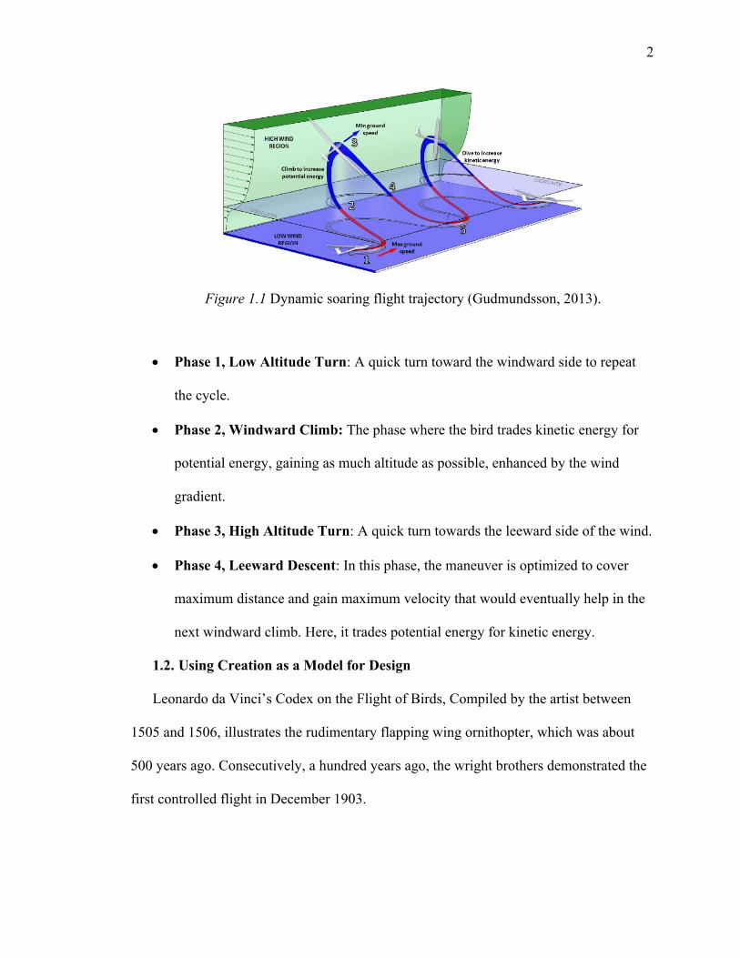
windward side and diving towards the leeward side in a cyclic fashion. The DS flight

path is made up of multiple phases as shown in Figure 1.1, and described below:

2

Figure 1.1 Dynamic soaring flight trajectory (Gudmundsson, 2013).

• Phase 1, Low Altitude Turn: A quick turn toward the windward side to repeat

the cycle.

• Phase 2, Windward Climb: The phase where the bird trades kinetic energy for

potential energy, gaining as much altitude as possible, enhanced by the wind

gradient.

• Phase 3, High Altitude Turn: A quick turn towards the leeward side of the wind.

• Phase 4, Leeward Descent: In this phase, the maneuver is optimized to cover

maximum distance and gain maximum velocity that would eventually help in the

next windward climb. Here, it trades potential energy for kinetic energy.

1.2. Using Creation as a Model for Design

Leonardo da Vinci’s Codex on the Flight of Birds, Compiled by the artist between

1505 and 1506, illustrates the rudimentary flapping wing ornithopter, which was about

500 years ago. Consecutively, a hundred years ago, the wright brothers demonstrated the

first controlled flight in December 1903.

3

This milestone led researchers and engineers to experiment with the multi-faceted

subject of aerodynamics, which resulted in the laws of aerodynamics that govern modern

flight. This led to the awe-inspiring realization that the laws existed ever since the

universe was put into place. The problem of achieving sustainable flight was already

solved by creation, billions of years ago.

Creation has been solving very complex mathematical problems for a very long time,

and this research only attempts to scratch the surface of the enormous possibilities of

biomimetic engineering design. The dynamic soaring maneuver is a flying technique that

is famously associated with the bird, Albatross. This phenomenon will be discussed

further in the subsequent sections. Some other significant examples of biomimetic design

are discussed below.

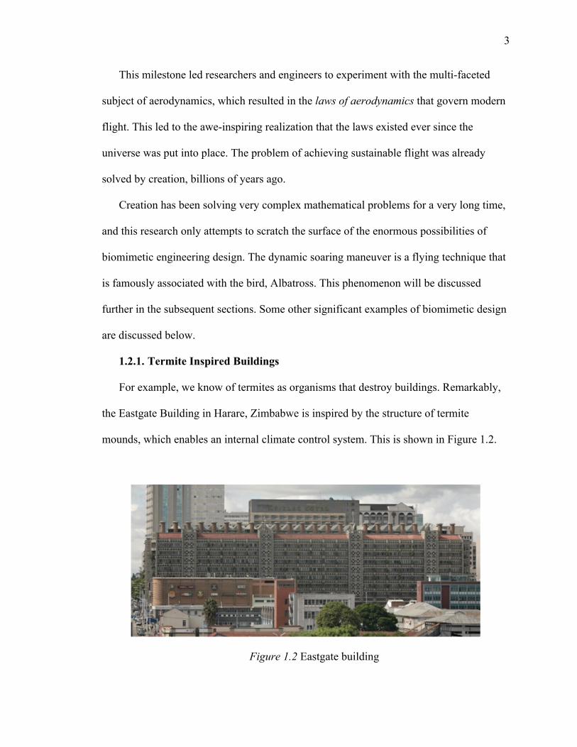
1.2.1. Termite Inspired Buildings

For example, we know of termites as organisms that destroy buildings. Remarkably,

the Eastgate Building in Harare, Zimbabwe is inspired by the structure of termite

mounds, which enables an internal climate control system. This is shown in Figure 1.2.

Figure 1.2 Eastgate building

4

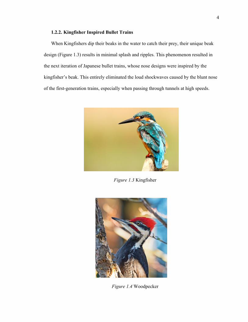
1.2.2. Kingfisher Inspired Bullet Trains

When Kingfishers dip their beaks in the water to catch their prey, their unique beak

design (Figure 1.3) results in minimal splash and ripples. This phenomenon resulted in

the next iteration of Japanese bullet trains, whose nose designs were inspired by the

kingfisher’s beak. This entirely eliminated the loud shockwaves caused by the blunt nose

of the first-generation trains, especially when passing through tunnels at high speeds.

Figure 1.3 Kingfisher

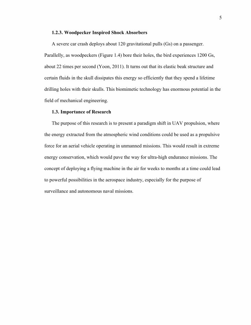
Figure 1.4 Woodpecker

5

1.2.3. Woodpecker Inspired Shock Absorbers

A severe car crash deploys about 120 gravitational pulls (Gs) on a passenger.

Parallelly, as woodpeckers (Figure 1.4) bore their holes, the bird experiences 1200 Gs,

about 22 times per second (Yoon, 2011). It turns out that its elastic beak structure and

certain fluids in the skull dissipates this energy so efficiently that they spend a lifetime

drilling holes with their skulls. This biomimetic technology has enormous potential in the

field of mechanical engineering.

1.3. Importance of Research

The purpose of this research is to present a paradigm shift in UAV propulsion, where

the energy extracted from the atmospheric wind conditions could be used as a propulsive

force for an aerial vehicle operating in unmanned missions. This would result in extreme

energy conservation, which would pave the way for ultra-high endurance missions. The

concept of deploying a flying machine in the air for weeks to months at a time could lead

to powerful possibilities in the aerospace industry, especially for the purpose of

surveillance and autonomous naval missions.

6

2. Review of the Relevant Literature

Dynamic soaring has been a focus of scientific inquiry for over 140 years. This

soaring technique, famously associated with the flight of the Albatross (Diomedea

exulans), was first recognized, and analyzed by Lord Rayleigh (1883). In its simplest

terms, the method is a repeated exchange of kinetic and potential energy in a non-

conservative force field, where the missing energy is extracted from the atmosphere.

An in-depth treatise of the mathematics of dynamic soaring is given in Cone’s

pioneering work, which starts off by making a statement that albatrosses can only achieve

cyclic dynamic soaring maneuvers in the presence of a brink and steady wind only

(1964). After years of observing the albatross’ unique flight maneuvers, Cone concluded

that the basic sequence of dynamic soaring consists of the 1) windward climb; 2) high-

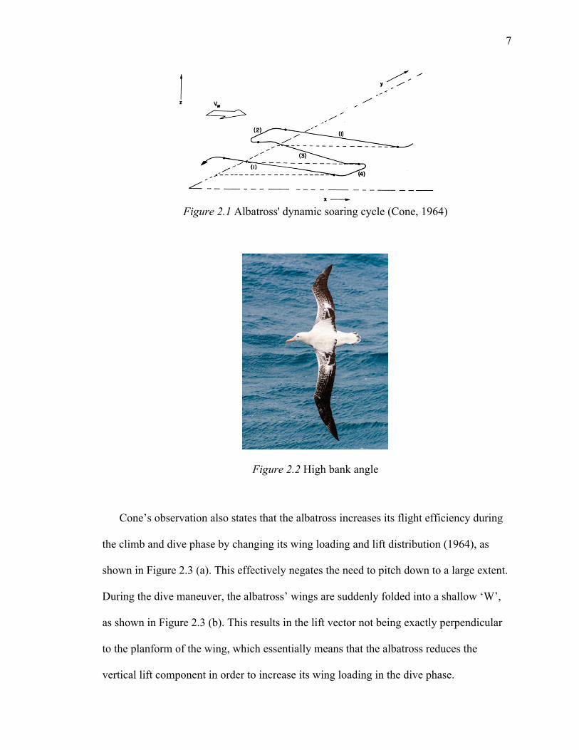
altitude turn; 3) leeward descent; and 4) the low altitude turn. This representation is

shown in Figure 2.1, that gives in-depth information on critical stages of this maneuver.

The windward climb is followed by a full 180° turn, allowing the bird to be pushed

by a tailwind. During this turn, the bird accelerates rapidly, achieving its state of

maximum kinetic energy at the end of this diving maneuver. Consecutively, the

windward climb starts off with maximum speed, which eventually curbs as the bird gains

altitude. It is also shown that both the high and low altitude turn are usually extremely

steep, where the albatross’s maximum bank angles are measured to be almost 90°, an

example of the bird’s extreme bank angle is shown in Figure 2.2.

7

Figure 2.1 Albatross' dynamic soaring cycle (Cone, 1964)

Figure 2.2 High bank angle

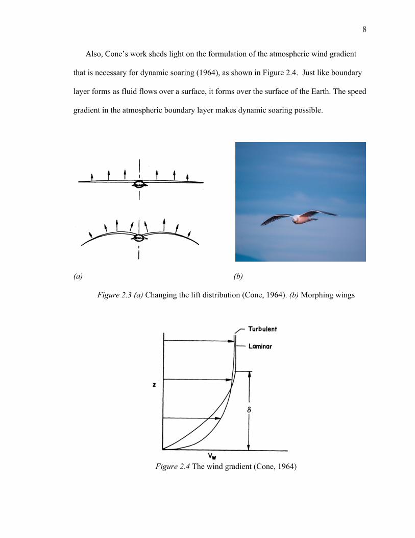
Cone’s observation also states that the albatross increases its flight efficiency during

the climb and dive phase by changing its wing loading and lift distribution (1964), as

shown in Figure 2.3 (a). This effectively negates the need to pitch down to a large extent.

During the dive maneuver, the albatross’ wings are suddenly folded into a shallow ‘W’,

as shown in Figure 2.3 (b). This results in the lift vector not being exactly perpendicular

to the planform of the wing, which essentially means that the albatross reduces the

vertical lift component in order to increase its wing loading in the dive phase.

8

Also, Cone’s work sheds light on the formulation of the atmospheric wind gradient

that is necessary for dynamic soaring (1964), as shown in Figure 2.4. Just like boundary

layer forms as fluid flows over a surface, it forms over the surface of the Earth. The speed

gradient in the atmospheric boundary layer makes dynamic soaring possible.

(a) (b)

Figure 2.3 (a) Changing the lift distribution (Cone, 1964). (b) Morphing wings

Figure 2.4 The wind gradient (Cone, 1964)

9

To this end, several bio-inspired flight-path optimization studies have been

implemented as reviewed by Gudmundsson (2019), where the possibilities of ridge

soaring is explored. The Lift Seeking-Sink Avoiding (LiSSA) algorithm developed in this

work attempts to evaluate the consequences of diverting from the shortest path from point

A to B to specifically seek the regions where extra lift can be gained in the sample

environment shown in Figure 2.5. This algorithm explores the possibilities of ridge

soaring for small unmanned aerial systems (sUAS) and estimates the cost of deviating

from the shortest path, in order to extract atmospheric energy.

Figure 2.5 A sample environment with the tallest mountain at 2400 m above sea level, with more than 7800 randomly allocated thermals (Gudmundsson, 2019).

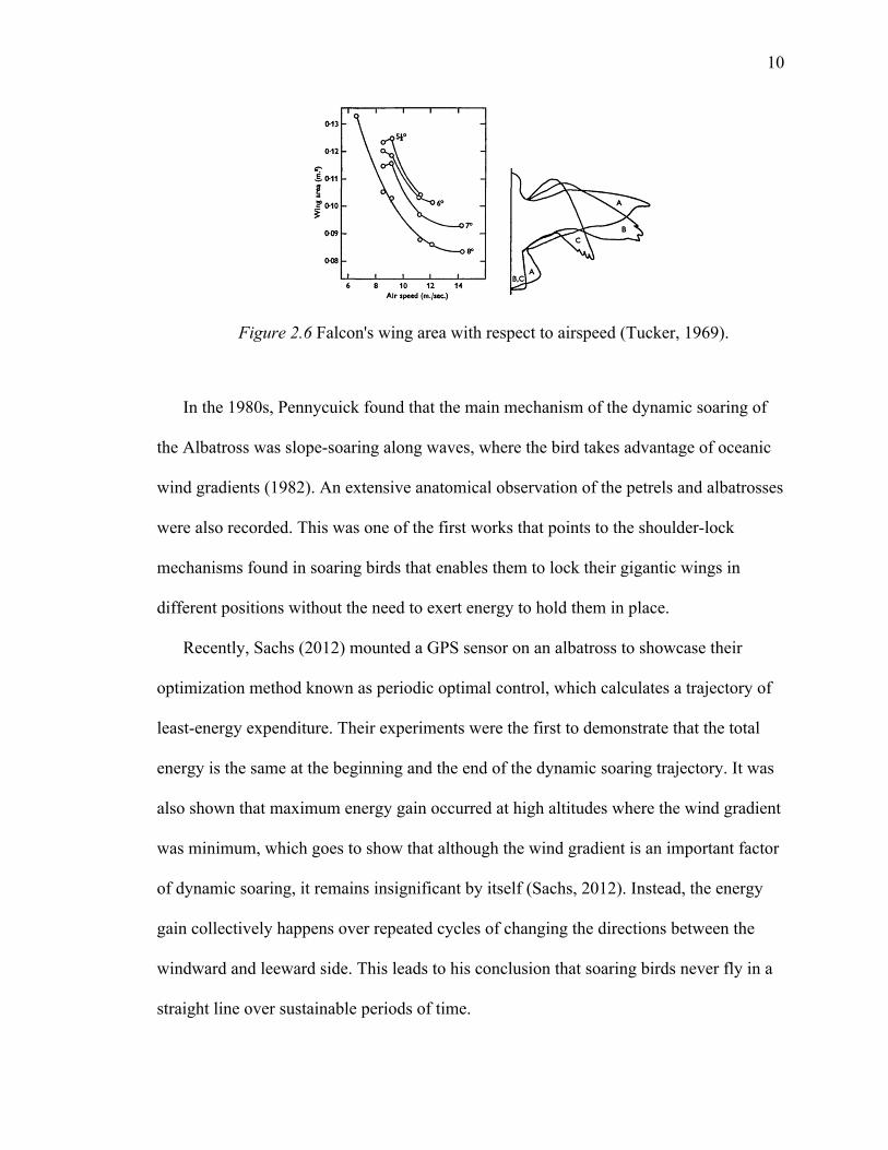
In the 1960s, Tucker and Parott (1969) concluded that only vertical changes in the

horizontal wind velocity component is needed to sustain dynamic soaring, upward wind

component is not required. This work attempts to investigate morphing wings, as it was

found that a laggar falcon (Falco jugger) reduces its wingspan, wing area and lift

coefficient with increasing airspeed. This establishes a pattern among soaring birds, that

incorporate some form of shape morphing in order to achieve maximum aerodynamic

efficiency. The wing area of this bird relative to its airspeed is shown in Figure 2.6.

10

Figure 2.6 Falcon's wing area with respect to airspeed (Tucker, 1969).

In the 1980s, Pennycuick found that the main mechanism of the dynamic soaring of

the Albatross was slope-soaring along waves, where the bird takes advantage of oceanic

wind gradients (1982). An extensive anatomical observation of the petrels and albatrosses

were also recorded. This was one of the first works that points to the shoulder-lock

mechanisms found in soaring birds that enables them to lock their gigantic wings in

different positions without the need to exert energy to hold them in place.

Recently, Sachs (2012) mounted a GPS sensor on an albatross to showcase their

optimization method known as periodic optimal control, which calculates a trajectory of

least-energy expenditure. Their experiments were the first to demonstrate that the total

energy is the same at the beginning and the end of the dynamic soaring trajectory. It was

also shown that maximum energy gain occurred at high altitudes where the wind gradient

was minimum, which goes to show that although the wind gradient is an important factor

of dynamic soaring, it remains insignificant by itself (Sachs, 2012). Instead, the energy

gain collectively happens over repeated cycles of changing the directions between the

windward and leeward side. This leads to his conclusion that soaring birds never fly in a

straight line over sustainable periods of time.

11

Recently, Williamson (2020) mounted GPS sensors on urban gulls and concluded that

they dynamically soar for 44% of their daily commute. This paper discusses the design of

the simulation environment that could simulate and quantify the energy gains reported in

the references above. With respect to mathematically modelling the dynamic soaring

flight path, Barnes (2004) studied the optimal flight path for the albatross to harvest

maximum energy from the wind. In his paper, he shows that such flight path enables the

albatross to fly for exceedingly long distances without spending almost any energy.

The results indicate that exploiting wind energy results in a significant reduction in

energy expenditure when compared to flying from Point A to B in a straight line. Sachs

and Grüter (2019) demonstrated that an unpowered glider could reach speeds up to 600

mph due to energy gain by dynamic soaring in a closed-circuit trajectory (Sachs, 2020). It

is an astonishing feat to accelerate a flying machine to 600 mph with no on-board energy

consumption. Finally, Deittert (2009) concludes that the ability to fly close to the surface

is a governing factor in extracting energy.

12

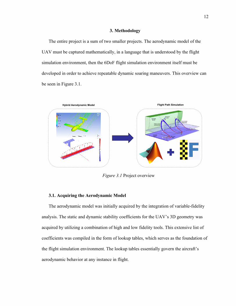
3. Methodology

The entire project is a sum of two smaller projects. The aerodynamic model of the

UAV must be captured mathematically, in a language that is understood by the flight

simulation environment, then the 6DoF flight simulation environment itself must be

developed in order to achieve repeatable dynamic soaring maneuvers. This overview can

be seen in Figure 3.1.

Figure 3.1 Project overview

3.1. Acquiring the Aerodynamic Model

The aerodynamic model was initially acquired by the integration of variable-fidelity

analysis. The static and dynamic stability coefficients for the UAV’s 3D geometry was

acquired by utilizing a combination of high and low fidelity tools. This extensive list of

coefficients was compiled in the form of lookup tables, which serves as the foundation of

the flight simulation environment. The lookup tables essentially govern the aircraft’s

aerodynamic behavior at any instance in flight.

Hybrid Aerodynamic Model Flight Path Simulation

13

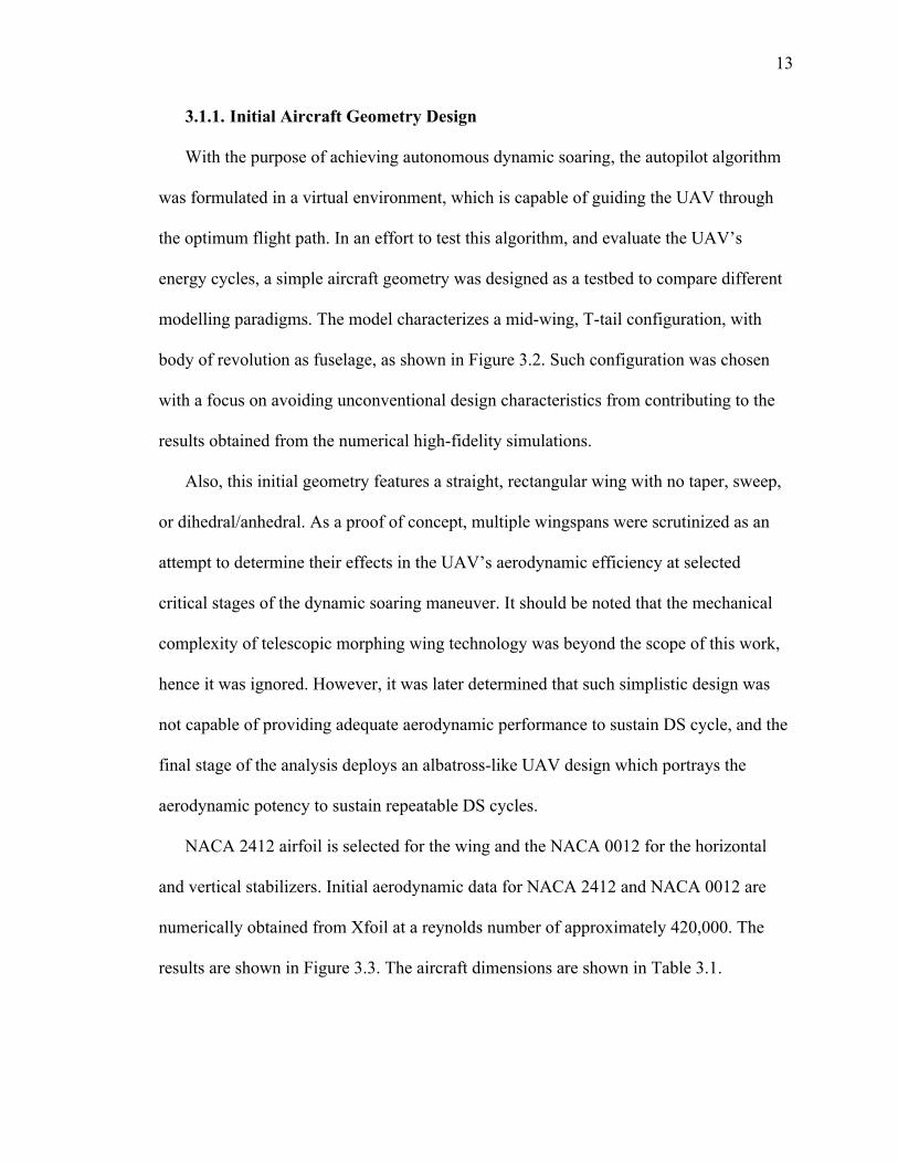
3.1.1. Initial Aircraft Geometry Design

With the purpose of achieving autonomous dynamic soaring, the autopilot algorithm

was formulated in a virtual environment, which is capable of guiding the UAV through

the optimum flight path. In an effort to test this algorithm, and evaluate the UAV’s

energy cycles, a simple aircraft geometry was designed as a testbed to compare different

modelling paradigms. The model characterizes a mid-wing, T-tail configuration, with

body of revolution as fuselage, as shown in Figure 3.2. Such configuration was chosen

with a focus on avoiding unconventional design characteristics from contributing to the

results obtained from the numerical high-fidelity simulations.

Also, this initial geometry features a straight, rectangular wing with no taper, sweep,

or dihedral/anhedral. As a proof of concept, multiple wingspans were scrutinized as an

attempt to determine their effects in the UAV’s aerodynamic efficiency at selected

critical stages of the dynamic soaring maneuver. It should be noted that the mechanical

complexity of telescopic morphing wing technology was beyond the scope of this work,

hence it was ignored. However, it was later determined that such simplistic design was

not capable of providing adequate aerodynamic performance to sustain DS cycle, and the

final stage of the analysis deploys an albatross-like UAV design which portrays the

aerodynamic potency to sustain repeatable DS cycles.

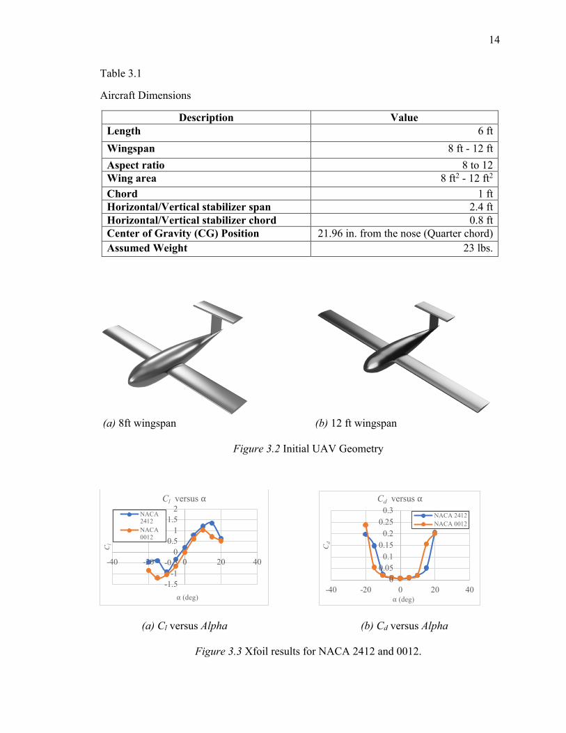
NACA 2412 airfoil is selected for the wing and the NACA 0012 for the horizontal

and vertical stabilizers. Initial aerodynamic data for NACA 2412 and NACA 0012 are

numerically obtained from Xfoil at a reynolds number of approximately 420,000. The

results are shown in Figure 3.3. The aircraft dimensions are shown in Table 3.1.

14

Table 3.1

Aircraft Dimensions

Description Value Length 6 ft Wingspan 8 ft - 12 ft Aspect ratio 8 to 12 Wing area 8 ft2 - 12 ft2

Chord 1 ft Horizontal/Vertical stabilizer span 2.4 ft Horizontal/Vertical stabilizer chord 0.8 ft Center of Gravity (CG) Position 21.96 in. from the nose (Quarter chord) Assumed Weight 23 lbs.

(a) 8ft wingspan (b) 12 ft wingspan

Figure 3.2 Initial UAV Geometry

(a) Cl versus Alpha (b) Cd versus Alpha

Figure 3.3 Xfoil results for NACA 2412 and 0012.

-1.5-1-0.500.511.52

-40 -20 0 20 40

Cl

⍺ (deg)

Cl versus ⍺NACA2412NACA0012

00.050.10.150.20.250.3

-40 -20 0 20 40

Cd

⍺ (deg)

Cd versus ⍺NACA 2412NACA 0012

15

3.1.2. Integration of Variable Fidelity Analysis

This section encompasses the analyses from a set of both low-fidelity and high-

fidelity tools to capture the aerodynamic model of the UAV. The variable fidelity tools

are deployed to calculate the coefficients of the aerodynamic forces and moments, and

the corresponding static and dynamic stability characteristics of the UAV.

3.1.2.1. SURFACES

SURFACES is an aircraft design software that resorts to the three-dimensional vortex

lattice method (VLM) to determine the airflow around the aircraft. Unlike the high-

fidelity CFD solver, a wide range of dynamic stability derivatives can be extracted from

the flow solution with the low-fidelity tool. The software calculates over 90 different

stability derivatives for the specified aircraft model. At the same time, the VLM solver

merely estimates the lift induced drag, as it is incapable of accounting for fluid viscosity,

especially at extreme angles of attack, which is where the inviscid methods fail to predict

the rapid increase in drag forces accompanying flow separation. Therefore, this is

augmented with the high-fidelity approach described in the next section.

3.1.2.2. ANSYS Fluent

ANSYS Fluent is a high-fidelity tool where different turbulence models are

implemented. This methodology is used to investigate the airflow over the UAV’s

geometry at extreme scenarios (i.e., high angles of attack followed by massive flow

separation) to obtain the aerodynamic derivatives. Simultaneously, the CFD solver is

used to validate the dynamic stability derivatives obtained from the low fidelity analysis.

The different turbulence models scrutinized are: 1) Spalart-Allmaras (1-equation); 2) K-ɛ

(2-equation); and 3) Detached Eddy Simulation (DES).

16

3.1.2.3. Numerical Implementation

The ultimate goal of the current study is to simulate the repeatable dynamic soaring

cycles with the quantification of kinetic and potential energies at critical stages. The

simulation will also measure the net energy gained or the net energy expended by the

UAV after each DS cycle and at the end of the complete flight. This virtual environment

would reveal some key characteristics like the minimum required wind shear, the

specifications of a control system capable of achieving perpetual DS, the efficiency of the

initial UAV’s design, etc. The general flight conditions employed in the variable-fidelity

analyses are shown in Table 3.2.

Table 3.2

General flight conditions

Description Value Altitude 0 ft - Sea Level Airspeed 20 m/s Pressure 1 atm. Density 1.225 Kg/m3

Temperature 15° C

3.1.2.3.1. ANSYS Fluent Model

This section describes the implementation of the high-fidelity, NAVIER-STOKES

solver for the purpose of capturing the static coefficients of the aerodynamic forces and

moments of the UAV by sweeping the geometry across various angles on all three axes.

The methodology used to implement the simulations on ANSYS Fluent is discussed

below, which includes the model geometry, the grid structure, and its implementation.

17

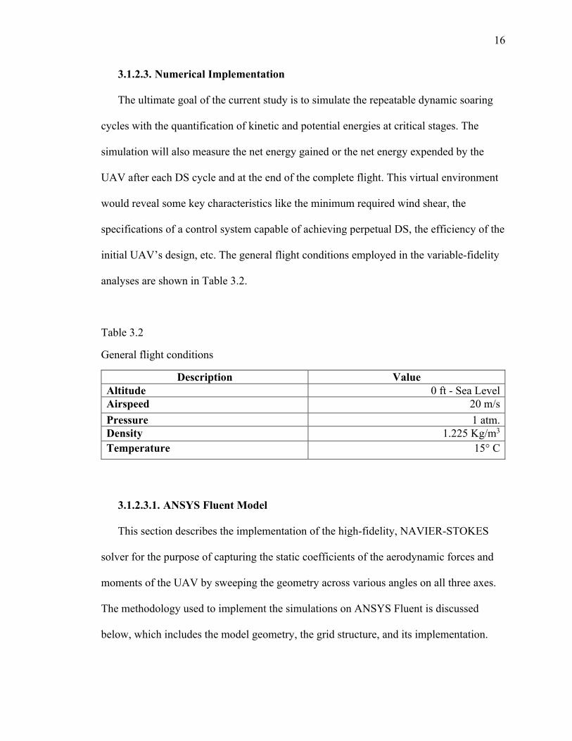
3.1.2.3.1.1. Model Geometry

The 3D model of the UAV is designed on Autodesk Fusion 360, a CAD / CAM

design software. As shown in Figure 3.4, a bounding box is required to define the fluid

domain around the UAV, and the corresponding reference values are shown in Table 3.3.

The inlet, outlet, and the walls of the bounding box are manually defined.

Figure 3.4 Bounding box for the fluid domain.

Table 3.3

Bounding box dimensions and reference values

Description Value Bounding box Length X 22.438 m Bounding box Length Y 20.528 m Bounding box Length Z 21.853 m Bounding box Volume 10066 m3

Area 0.743 m2 - 1.115 m2 Density 1.225 kg/m2 Reference length 0.305 m (Chord length) Temperature 288 K Velocity 20 m/s Viscosity 1.7894 ´ 10-5 kg/m-s Ratio of specific heats 1.4

18

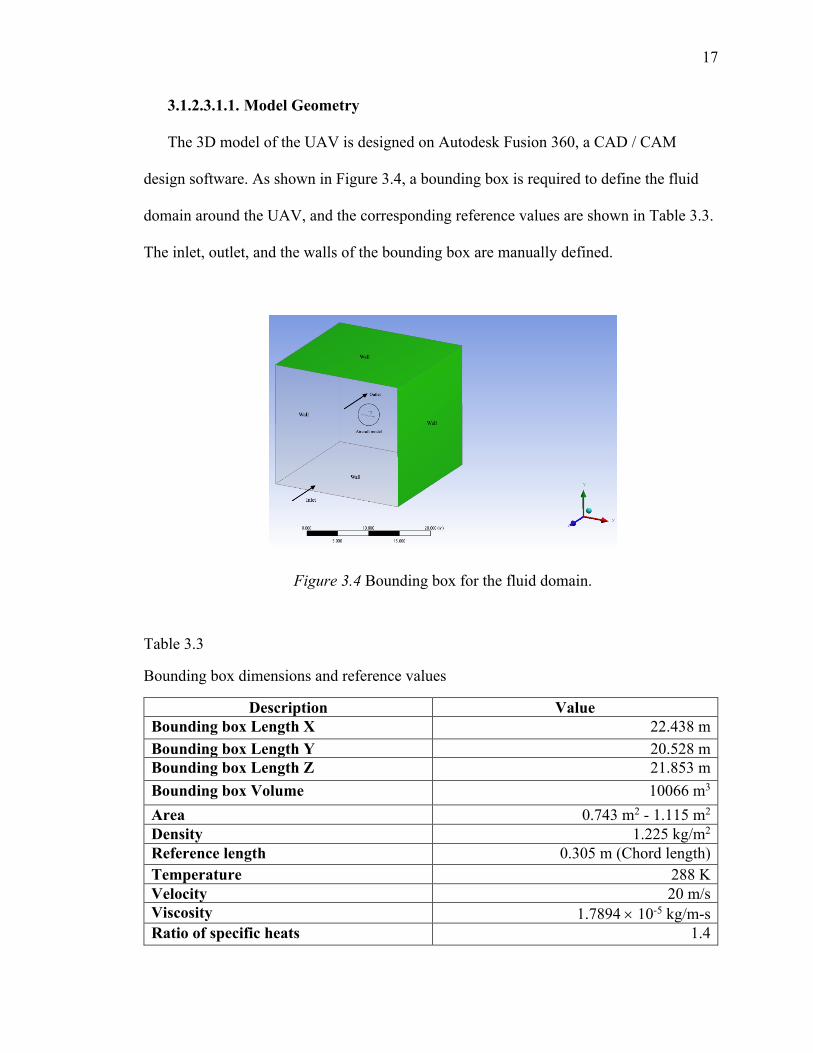
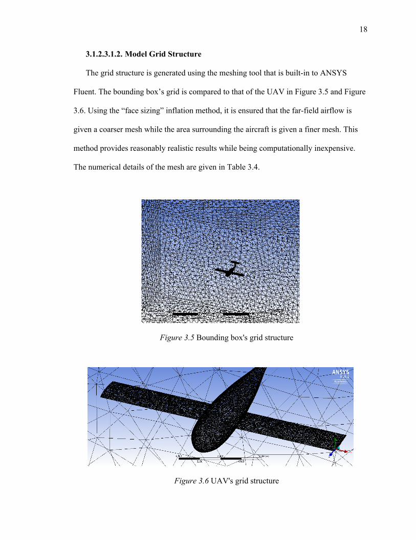
3.1.2.3.1.2. Model Grid Structure

The grid structure is generated using the meshing tool that is built-in to ANSYS

Fluent. The bounding box’s grid is compared to that of the UAV in Figure 3.5 and Figure

3.6. Using the “face sizing” inflation method, it is ensured that the far-field airflow is

given a coarser mesh while the area surrounding the aircraft is given a finer mesh. This

method provides reasonably realistic results while being computationally inexpensive.

The numerical details of the mesh are given in Table 3.4.

Figure 3.5 Bounding box's grid structure

Figure 3.6 UAV's grid structure

19

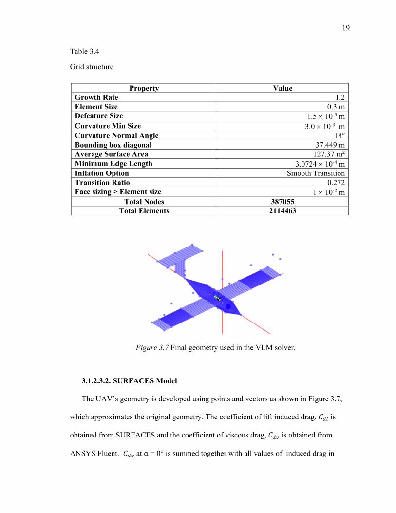
Table 3.4

Grid structure

Figure 3.7 Final geometry used in the VLM solver.

3.1.2.3.2. SURFACES Model

The UAV’s geometry is developed using points and vectors as shown in Figure 3.7,

which approximates the original geometry. The coefficient of lift induced drag, -23 is

obtained from SURFACES and the coefficient of viscous drag, -24 is obtained from

ANSYS Fluent. -24 at ⍺ = 0° is summed together with all values of induced drag in

Property Value Growth Rate 1.2 Element Size 0.3 m Defeature Size 1.5 ´ 10-3 m Curvature Min Size 3.0 ´ 10-3 m Curvature Normal Angle 18° Bounding box diagonal 37.449 m Average Surface Area 127.37 m2

Minimum Edge Length 3.0724 ´ 10-4 m Inflation Option Smooth Transition Transition Ratio 0.272 Face sizing > Element size 1 ´ 10-2 m

Total Nodes 387055 Total Elements 2114463

20

order to estimate an approximated total coefficient of drag. The VLM solver computes

the pressure values at every panel of the approximated geometry. The forces, moments

and dynamic stability derivatives are extracted from this VLM solution.

3.1.3. Selecting the Turbulence Model

The results from the isolated-wing simulations and the complete aircraft simulations

are first examined and validated in order to select the appropriate turbulence model for

the subsequent analyses. The most suitable model would be the one that closely resemble

reality with the lest computational cost.

3.1.3.1. Methodology to Compare the Turbulence Models

ANSYS Fluent has a variety of turbulence models for various fluid dynamics

applications. Depending on the nature of the problem, the turbulence models can be

chosen, but this must go through a detailed validation process. The K-Epsilon, Spallart-

Allmaras, and detached eddy simulations models were compared and the most

appropriate model for this analysis was chosen.

3.1.3.1.1. Isolated Wing Simulation

The 3D model of the wing is isolated from rest of the UAV’s and it is studied using

CFD simulations in order to prevent the aircraft’s complex geometry in playing a role in

selecting the best turbulence model for this specific study. This is done by sweeping the

wing over various angles of attack and the corresponding coefficient of lift is plotted and

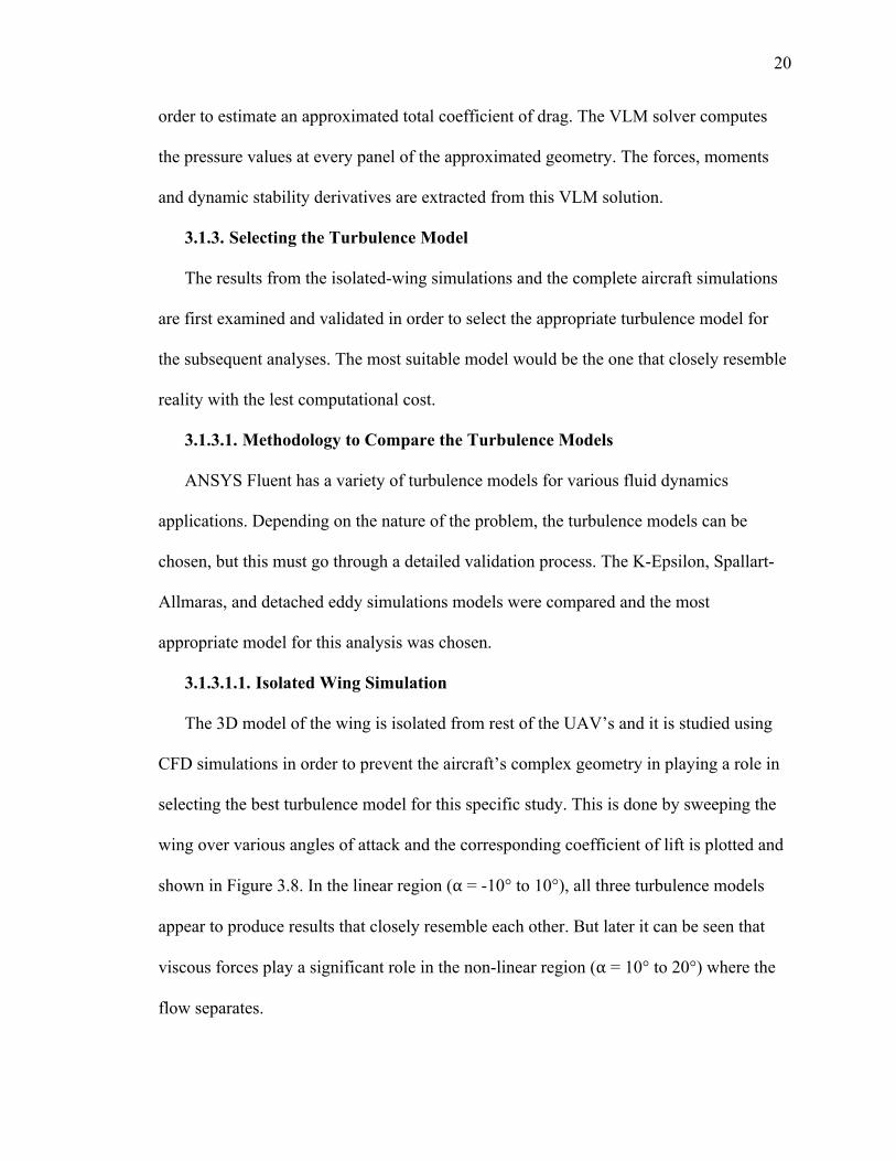
shown in Figure 3.8. In the linear region (⍺ = -10° to 10°), all three turbulence models

appear to produce results that closely resemble each other. But later it can be seen that

viscous forces play a significant role in the non-linear region (⍺ = 10° to 20°) where the

flow separates.

21

Time after time, the K-ɛ turbulence model overestimates the coefficient of lift, which

reveals the model’s inability to accurately account for the viscous forces. The DES

simulations predict the lowest CL, followed by k-ɛ and the SA model. In addition to the

three turbulence models, with a goal of validating them, the results are compared with the

experimental wind tunnel data for the NACA 2412 airfoil’s sectional lift coefficient

(Seetharam, 1977) and the NACA 2412 wing’s total lift coefficient data (Saha, 1999).

These effects are further studied and comprehended by running the same simulations for

the entire aircraft.

Figure 3.8 CL versus Alpha of the isolated wing.

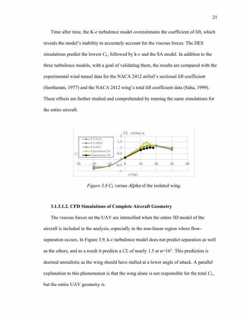
3.1.3.1.2. CFD Simulations of Complete Aircraft Geometry

The viscous forces on the UAV are intensified when the entire 3D model of the

aircraft is included in the analysis, especially in the non-linear region where flow-

separation occurs. In Figure 3.9, k-ɛ turbulence model does not predict separation as well

as the others, and as a result it predicts a CL of nearly 1.5 at ⍺=16°. This prediction is

deemed unrealistic as the wing should have stalled at a lower angle of attack. A parallel

explanation to this phenomenon is that the wing alone is not responsible for the total CL,

but the entire UAV geometry is.

-1-0.500.511.52

-30 -20 -10 0 10 20 30 40

CL

⍺ (deg)

CL versus ⍺8 ft (S-A)8 ft (DES)8 ft (KE)Experimental 2DExperimental 3D

22

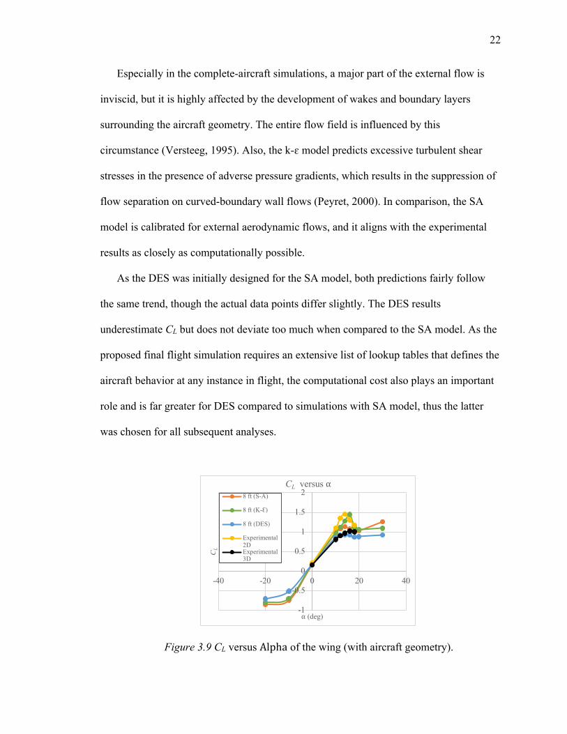
Especially in the complete-aircraft simulations, a major part of the external flow is

inviscid, but it is highly affected by the development of wakes and boundary layers

surrounding the aircraft geometry. The entire flow field is influenced by this

circumstance (Versteeg, 1995). Also, the k-ɛ model predicts excessive turbulent shear

stresses in the presence of adverse pressure gradients, which results in the suppression of

flow separation on curved-boundary wall flows (Peyret, 2000). In comparison, the SA

model is calibrated for external aerodynamic flows, and it aligns with the experimental

results as closely as computationally possible.

As the DES was initially designed for the SA model, both predictions fairly follow

the same trend, though the actual data points differ slightly. The DES results

underestimate CL but does not deviate too much when compared to the SA model. As the

proposed final flight simulation requires an extensive list of lookup tables that defines the

aircraft behavior at any instance in flight, the computational cost also plays an important

role and is far greater for DES compared to simulations with SA model, thus the latter

was chosen for all subsequent analyses.

Figure 3.9 CL versus Alpha of the wing (with aircraft geometry).

-1

-0.5

0

0.5

1

1.5

2

-40 -20 0 20 40

CL

⍺ (deg)

CL versus ⍺8 ft (S-A)

8 ft (K-Ɛ)

8 ft (DES)

Experimental2DExperimental3D

23

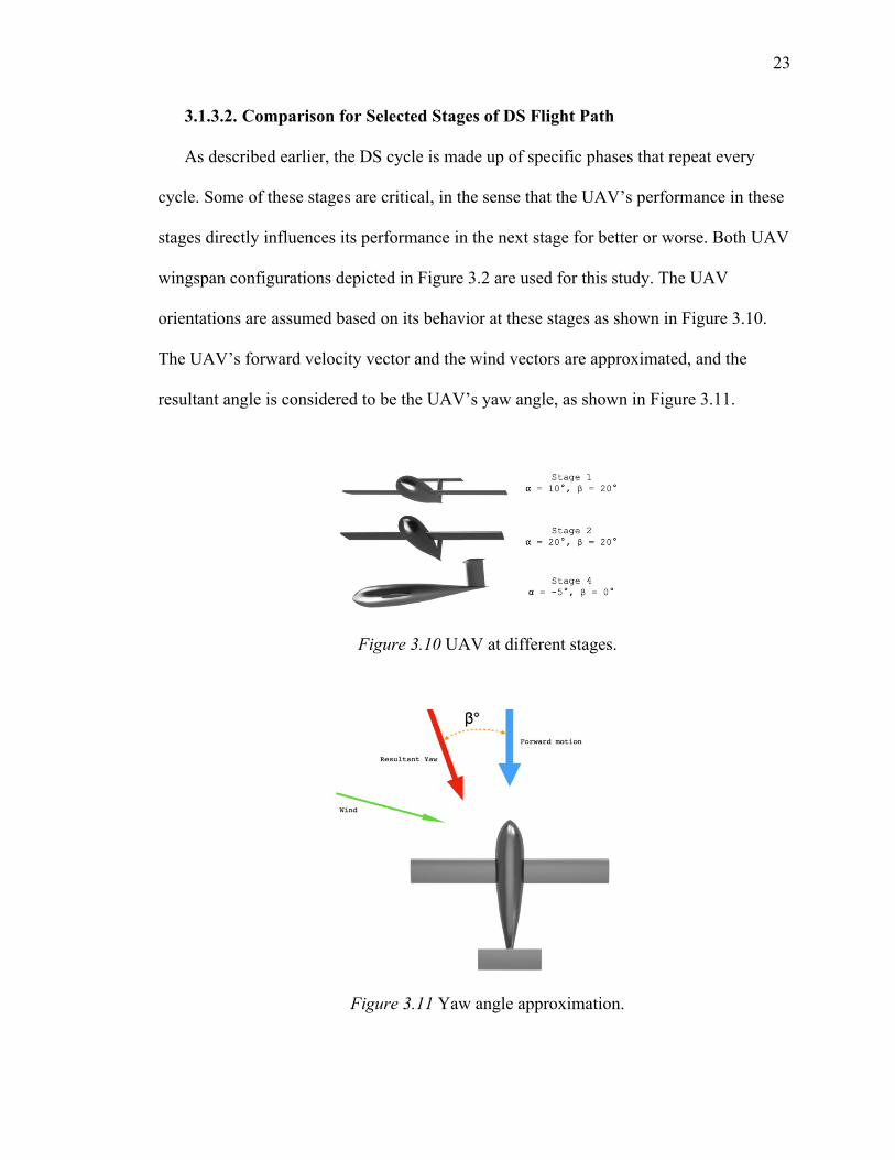
3.1.3.2. Comparison for Selected Stages of DS Flight Path

As described earlier, the DS cycle is made up of specific phases that repeat every

cycle. Some of these stages are critical, in the sense that the UAV’s performance in these

stages directly influences its performance in the next stage for better or worse. Both UAV

wingspan configurations depicted in Figure 3.2 are used for this study. The UAV

orientations are assumed based on its behavior at these stages as shown in Figure 3.10.

The UAV’s forward velocity vector and the wind vectors are approximated, and the

resultant angle is considered to be the UAV’s yaw angle, as shown in Figure 3.11.

Figure 3.10 UAV at different stages.

Figure 3.11 Yaw angle approximation.

24

(a) (b)

(c) (d)

(e)

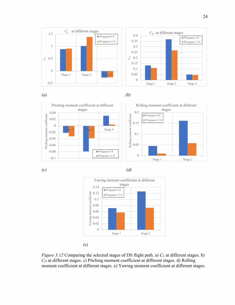
Figure 3.12 Comparing the selected stages of DS flight path. a) CL at different stages. b) CD at different stages. c) Pitching moment coefficient at different stages. d) Rolling moment coefficient at different stages. e) Yawing moment coefficient at different stages.

-0.5

0

0.5

1

1.5

Stage 1 Stage 2 Stage 4

CL

CL at different stagesWingspan 8 ft

Wingspan 12 ft

00.050.10.150.20.250.30.350.4


CD

CD at different stagesWingspan 8 ftWingspan 12 ft

-0.1

-0.08

-0.06

-0.04

-0.02

0

0.02

0.04


Pitc

hing

mom

ent c

oeff

icie

nt

Pitching moment coefficient at different stages

Wingspan 8 ftWingspan 12 ft 0

0.05

0.1

0.15

0.2

Stage 1 Stage 2

Rol

ling

mom

ent c

oeff

icie

nt

Rolling moment coefficient at different stages

Wingspan 8 ft

Wingspan 12 ft

0

0.02

0.04

0.06

0.08

0.1

0.12

0.14

Stage 1 Stage 2

Yaw

ing

mom

ent c

oeffi

cien

t

Yawing moment coefficient at different stages

Wingspan 8 ft

Wingspan 12 ft

25

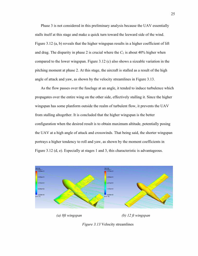
Phase 3 is not considered in this preliminary analysis because the UAV essentially

stalls itself at this stage and make a quick turn toward the leeward side of the wind.

Figure 3.12 (a, b) reveals that the higher wingspan results in a higher coefficient of lift

and drag. The disparity in phase 2 is crucial where the CL is about 40% higher when

compared to the lower wingspan. Figure 3.12 (c) also shows a sizeable variation in the

pitching moment at phase 2. At this stage, the aircraft is stalled as a result of the high

angle of attack and yaw, as shown by the velocity streamlines in Figure 3.13.

As the flow passes over the fuselage at an angle, it tended to induce turbulence which

propagates over the entire wing on the other side, effectively stalling it. Since the higher

wingspan has some planform outside the realm of turbulent flow, it prevents the UAV

from stalling altogether. It is concluded that the higher wingspan is the better

configuration when the desired result is to obtain maximum altitude, potentially posing

the UAV at a high angle of attack and crosswinds. That being said, the shorter wingspan

portrays a higher tendency to roll and yaw, as shown by the moment coefficients in

Figure 3.12 (d, e). Especially at stages 1 and 3, this characteristic is advantageous.

(a) 8ft wingspan (b) 12 ft wingspan

Figure 3.13 Velocity streamlines

26

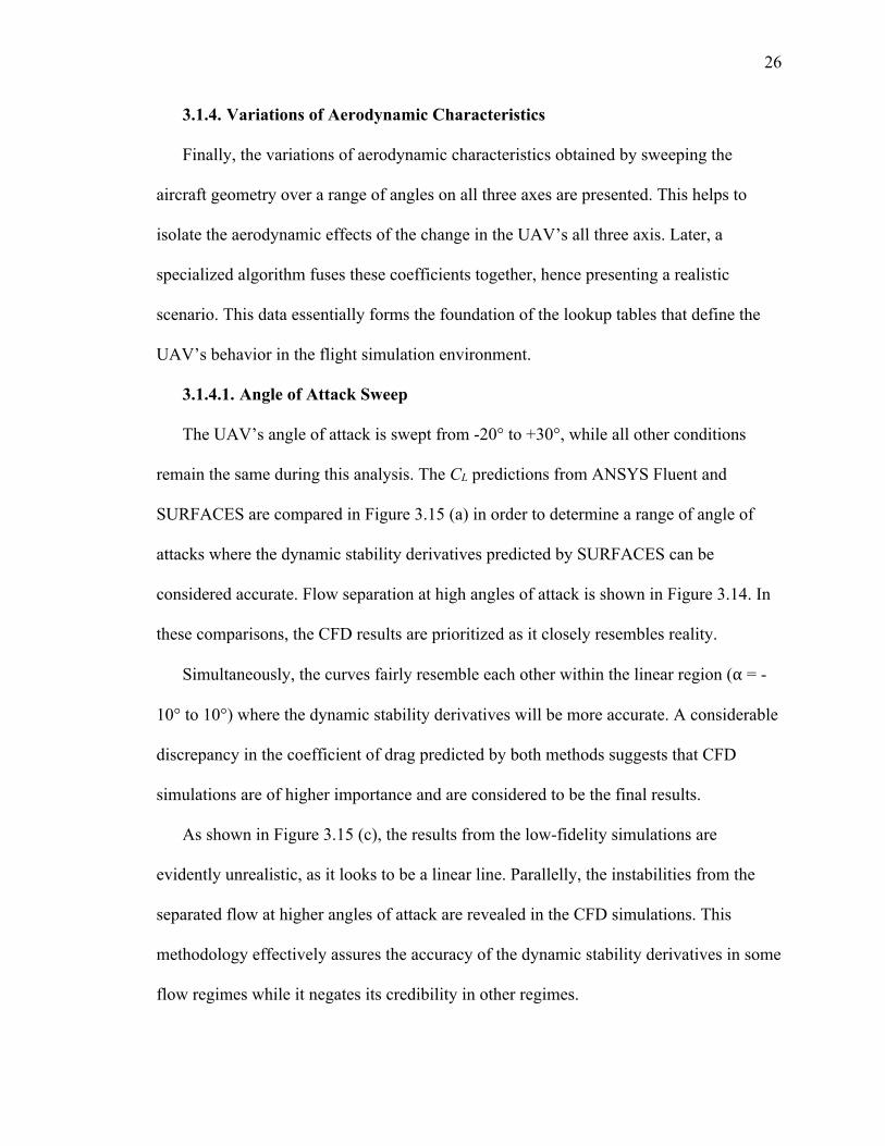
3.1.4. Variations of Aerodynamic Characteristics

Finally, the variations of aerodynamic characteristics obtained by sweeping the

aircraft geometry over a range of angles on all three axes are presented. This helps to

isolate the aerodynamic effects of the change in the UAV’s all three axis. Later, a

specialized algorithm fuses these coefficients together, hence presenting a realistic

scenario. This data essentially forms the foundation of the lookup tables that define the

UAV’s behavior in the flight simulation environment.

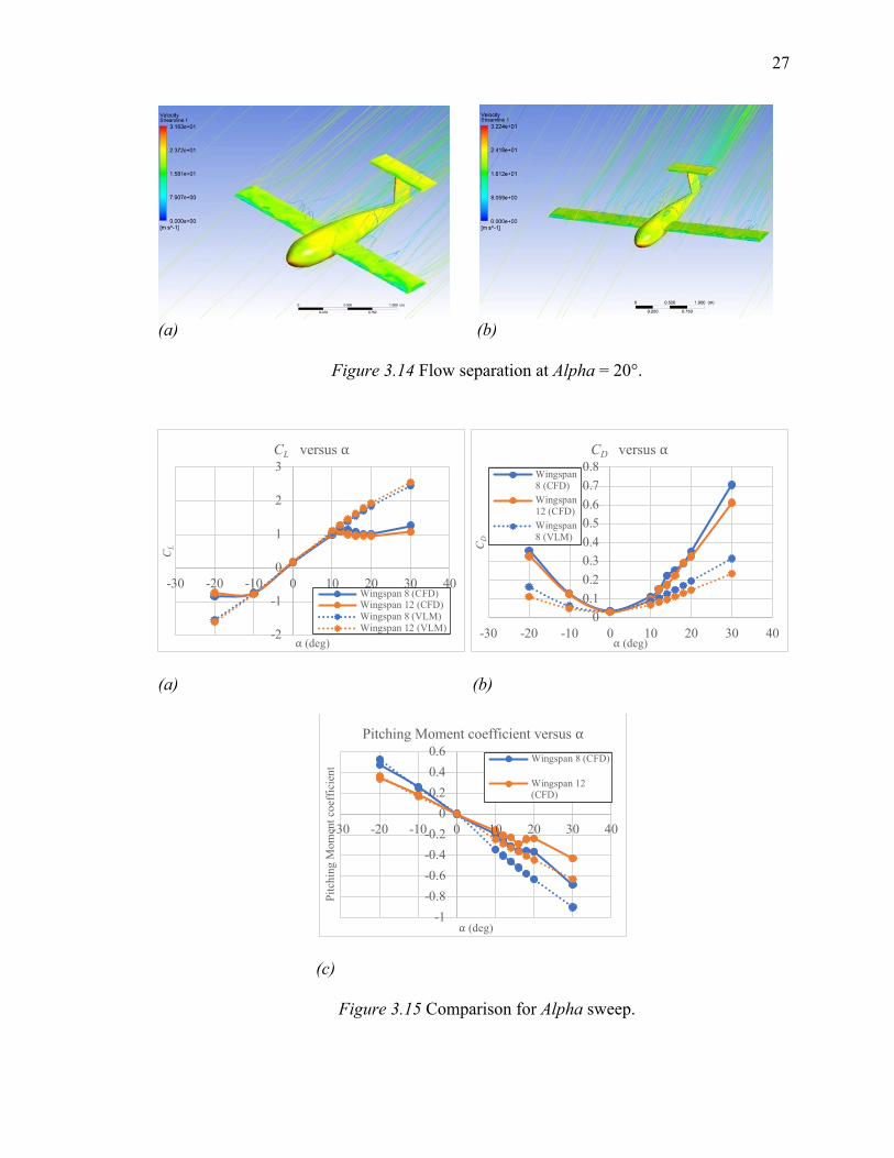
3.1.4.1. Angle of Attack Sweep

The UAV’s angle of attack is swept from -20° to +30°, while all other conditions

remain the same during this analysis. The CL predictions from ANSYS Fluent and

SURFACES are compared in Figure 3.15 (a) in order to determine a range of angle of

attacks where the dynamic stability derivatives predicted by SURFACES can be

considered accurate. Flow separation at high angles of attack is shown in Figure 3.14. In

these comparisons, the CFD results are prioritized as it closely resembles reality.

Simultaneously, the curves fairly resemble each other within the linear region (⍺ = -

10° to 10°) where the dynamic stability derivatives will be more accurate. A considerable

discrepancy in the coefficient of drag predicted by both methods suggests that CFD

simulations are of higher importance and are considered to be the final results.

As shown in Figure 3.15 (c), the results from the low-fidelity simulations are

evidently unrealistic, as it looks to be a linear line. Parallelly, the instabilities from the

separated flow at higher angles of attack are revealed in the CFD simulations. This

methodology effectively assures the accuracy of the dynamic stability derivatives in some

flow regimes while it negates its credibility in other regimes.

27

(a) (b)

Figure 3.14 Flow separation at Alpha = 20°.

(a) (b)

(c)

Figure 3.15 Comparison for Alpha sweep.

-2

-1

0

1

2

3

-30 -20 -10 0 10 20 30 40

CL

⍺ (deg)

CL versus ⍺

Wingspan 8 (CFD)Wingspan 12 (CFD)Wingspan 8 (VLM)Wingspan 12 (VLM)

00.10.20.30.40.50.60.70.8

-30 -20 -10 0 10 20 30 40

CD

⍺ (deg)

CD versus ⍺Wingspan8 (CFD)Wingspan12 (CFD)Wingspan8 (VLM)

-1-0.8-0.6-0.4-0.200.20.40.6

-30 -20 -10 0 10 20 30 40

Pitc

hing

Mom

ent c

oeff

icie

nt

⍺ (deg)

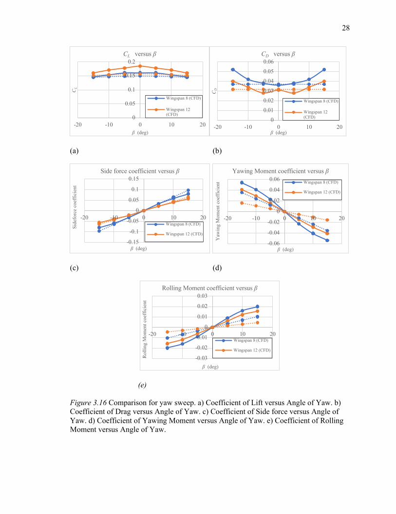
Pitching Moment coefficient versus ⍺Wingspan 8 (CFD)

Wingspan 12(CFD)

28

(a) (b)

(c) (d)

(e)

Figure 3.16 Comparison for yaw sweep. a) Coefficient of Lift versus Angle of Yaw. b) Coefficient of Drag versus Angle of Yaw. c) Coefficient of Side force versus Angle of Yaw. d) Coefficient of Yawing Moment versus Angle of Yaw. e) Coefficient of Rolling Moment versus Angle of Yaw.

0

0.05

0.1

0.15

0.2

-20 -10 0 10 20

CL

β (deg)

CL versus β

Wingspan 8 (CFD)

Wingspan 12(CFD)

00.010.020.030.040.050.06

-20 -10 0 10 20

CD

β (deg)

CD versus β

Wingspan 8 (CFD)

Wingspan 12(CFD)

-0.15

-0.1

-0.05

0

0.05

0.1

0.15

-20 -10 0 10 20

Side

forc

e co

effic

ient

β (deg)

Side force coefficient versus β

Wingspan 8 (CFD)

Wingspan 12 (CFD)

-0.06

-0.04

-0.02

0

0.02

0.04

0.06

-20 -10 0 10 20Y

awin

g M

omen

t coe

ffici

ent

β (deg)

Yawing Moment coefficient versus βWingspan 8 (CFD)

Wingspan 12 (CFD)

-0.03

-0.02

-0.01

0

0.01

0.02

0.03

-20 -10 0 10 20

Rol

ling

Mom

ent c

oeff

icie

nt

β (deg)

Rolling Moment coefficient versus β

Wingspan 8 (CFD)

Wingspan 12 (CFD)

29

(a) (b)

(c)

Figure 3.17 Comparison for roll sweep. a) Coefficient of Lift versus Angle of Roll. b) Coefficient of Side force versus Angle of Roll. c) Coefficient of Yawing Moment versus Angle of Roll.

3.1.4.2. Yaw Sweep

The angle of yaw is swept from -15° to +15°. All other conditions remain the same

during the analysis. To reduce computational costs, the analysis is done exclusively on

the positive angles, and the signs are reversed for the negative angles of the same

magnitude. The aircraft’s yaw angle plays an important role in both the coefficient of lift

and drag as shown in Figure 3.16 (a, b). The corresponding coefficients are shown in

Figure 3.16 (c, d, and e).

0

0.05

0.1

0.15

0.2

-30 -20 -10 0 10 20 30

CL

ɣ (deg)

CL versus ɣ

Wingspan 8

Wingspan 12

-0.08-0.06-0.04-0.02

00.020.040.060.08

-30 -20 -10 0 10 20 30

Cfx

(Sid

efor

ce)

ɣ (deg)

Side force coefficient versus ɣ

Wingspan 8

Wingspan 12

-0.004-0.003-0.002-0.001

00.0010.0020.0030.004

-30 -20 -10 0 10 20 30

Yaw

ing

Mom

ent c

oeffi

cien

t

ɣ (deg)

Yawing Moment coefficient versus ɣWingspan 8Wingspan 12

30

3.1.4.3. Roll Sweep

The angle of roll is swept from -20° to +20°. All other conditions remain the same

during the analysis. The signs are reversed for the negative angles for the directional

stability, as the analysis is performed only for the positive angles for the same reason as

reducing computational costs. The VLM solver’s static stability derivatives in the roll

axis turned out to be insignificant, hence they are ignored for the purposes of this

analysis. Consecutively, the CFD results as shown in Figure 3.17 are chosen to be

implemented in the final flight simulation.

3.1.4.4. Dynamic Stability Derivatives

The dynamic stability derivatives for this UAV are obtained from SURFACES as

described in section IV-B. The values are also validated using the proposed hybrid

aerodynamic model that integrates the variable fidelity of SURFACES and ANSYS

Fluent. An extensive list of dynamic stability derivatives is listed in Appendix A.

According to the coordinate system that SURFACES implements, the X axis is

longitudinal, Y axis is lateral, and the Z axis is vertical.

3.2. Building the Flight Simulation Environment

The flight simulation environment encapsulates the aircraft dynamics and the control

systems which were developed from the ground up using the graphical programming

language, Simulink. This design paradigm allows the development of complex systems

visually in the form of blocks (or subsystems) that are relatively easy to debug, when

compared to conventional programming languages. A simple illustration of this system is

shown in Figure 3.18, which also shows an overview of the Simulink environment

developed for this study.

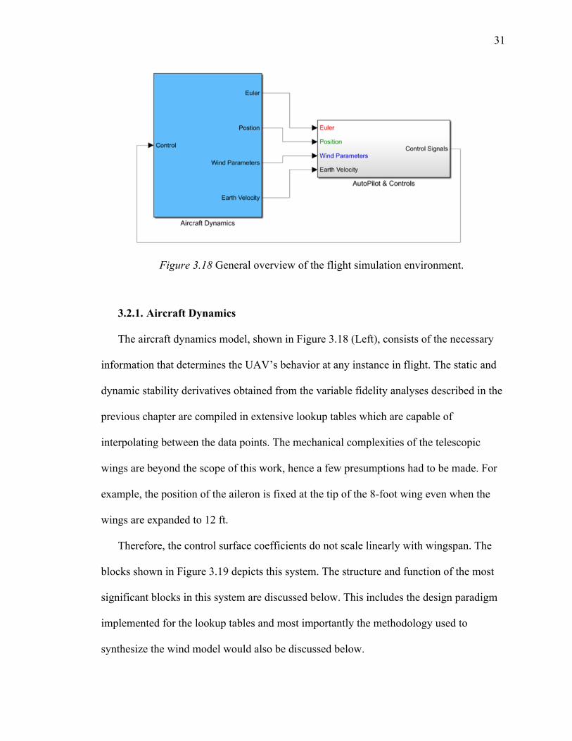
31

Figure 3.18 General overview of the flight simulation environment.

3.2.1. Aircraft Dynamics

The aircraft dynamics model, shown in Figure 3.18 (Left), consists of the necessary

information that determines the UAV’s behavior at any instance in flight. The static and

dynamic stability derivatives obtained from the variable fidelity analyses described in the

previous chapter are compiled in extensive lookup tables which are capable of

interpolating between the data points. The mechanical complexities of the telescopic

wings are beyond the scope of this work, hence a few presumptions had to be made. For

example, the position of the aileron is fixed at the tip of the 8-foot wing even when the

wings are expanded to 12 ft.

Therefore, the control surface coefficients do not scale linearly with wingspan. The

blocks shown in Figure 3.19 depicts this system. The structure and function of the most

significant blocks in this system are discussed below. This includes the design paradigm

implemented for the lookup tables and most importantly the methodology used to

synthesize the wind model would also be discussed below.

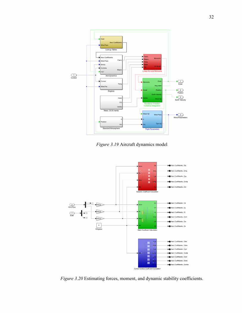
32

Figure 3.19 Aircraft dynamics model

Figure 3.20 Estimating forces, moment, and dynamic stability coefficients.

33

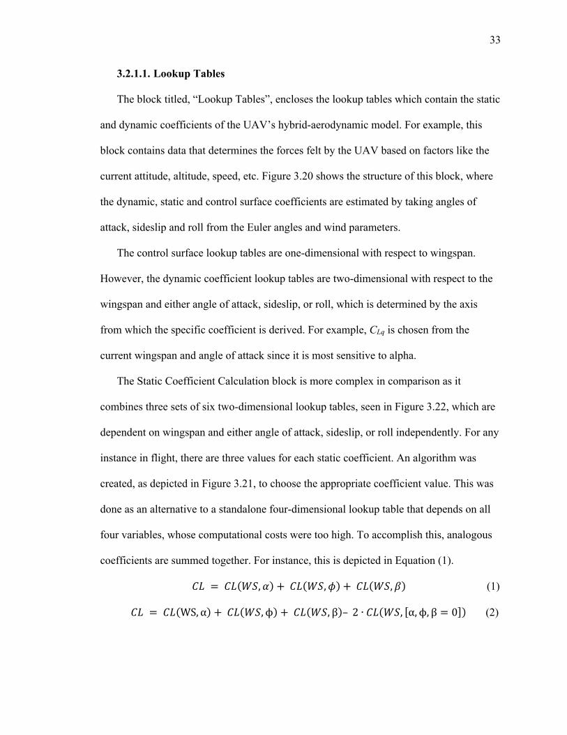
3.2.1.1. Lookup Tables

The block titled, “Lookup Tables”, encloses the lookup tables which contain the static

and dynamic coefficients of the UAV’s hybrid-aerodynamic model. For example, this

block contains data that determines the forces felt by the UAV based on factors like the

current attitude, altitude, speed, etc. Figure 3.20 shows the structure of this block, where

the dynamic, static and control surface coefficients are estimated by taking angles of

attack, sideslip and roll from the Euler angles and wind parameters.

The control surface lookup tables are one-dimensional with respect to wingspan.

However, the dynamic coefficient lookup tables are two-dimensional with respect to the

wingspan and either angle of attack, sideslip, or roll, which is determined by the axis

from which the specific coefficient is derived. For example, CLq is chosen from the

current wingspan and angle of attack since it is most sensitive to alpha.

The Static Coefficient Calculation block is more complex in comparison as it

combines three sets of six two-dimensional lookup tables, seen in Figure 3.22, which are

dependent on wingspan and either angle of attack, sideslip, or roll independently. For any

instance in flight, there are three values for each static coefficient. An algorithm was

created, as depicted in Figure 3.21, to choose the appropriate coefficient value. This was

done as an alternative to a standalone four-dimensional lookup table that depends on all

four variables, whose computational costs were too high. To accomplish this, analogous

coefficients are summed together. For instance, this is depicted in Equation (1).

-0 = -0(/3, 4) + -0(/3, 7) + -0(/3, 8) (1)

-0 = -0(WS, α) + -0(/3,ϕ) + -0(/3, β)– 2 ∙ -0(/3, [α, ϕ, β = 0]) (2)

34

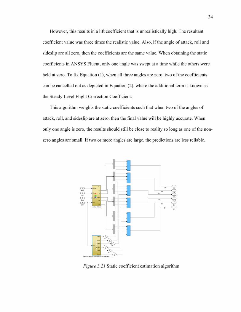
However, this results in a lift coefficient that is unrealistically high. The resultant

coefficient value was three times the realistic value. Also, if the angle of attack, roll and

sideslip are all zero, then the coefficients are the same value. When obtaining the static

coefficients in ANSYS Fluent, only one angle was swept at a time while the others were

held at zero. To fix Equation (1), when all three angles are zero, two of the coefficients

can be cancelled out as depicted in Equation (2), where the additional term is known as

the Steady Level Flight Correction Coefficient.

This algorithm weights the static coefficients such that when two of the angles of

attack, roll, and sideslip are at zero, then the final value will be highly accurate. When

only one angle is zero, the results should still be close to reality so long as one of the non-

zero angles are small. If two or more angles are large, the predictions are less reliable.

Figure 3.21 Static coefficient estimation algorithm

35

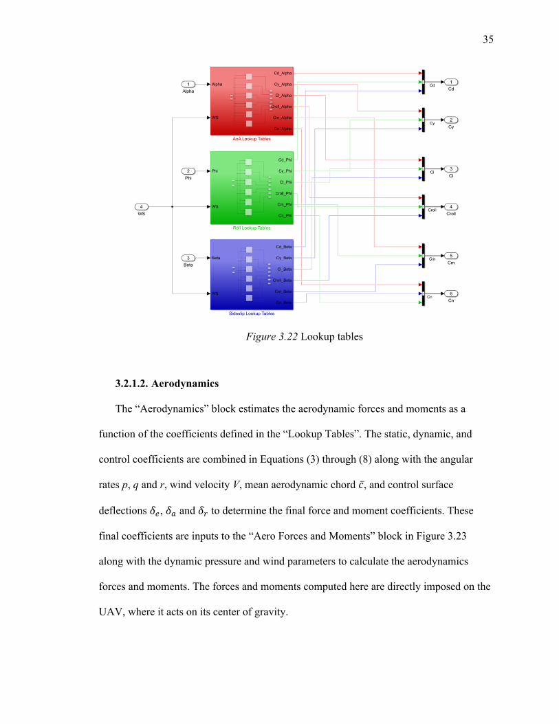
Figure 3.22 Lookup tables

3.2.1.2. Aerodynamics

The “Aerodynamics” block estimates the aerodynamic forces and moments as a

function of the coefficients defined in the “Lookup Tables”. The static, dynamic, and

control coefficients are combined in Equations (3) through (8) along with the angular

rates p, q and r, wind velocity V, mean aerodynamic chord +̅, and control surface

deflections *!, *# and *" to determine the final force and moment coefficients. These

final coefficients are inputs to the “Aero Forces and Moments” block in Figure 3.23

along with the dynamic pressure and wind parameters to calculate the aerodynamics

forces and moments. The forces and moments computed here are directly imposed on the

UAV, where it acts on its center of gravity.

36

-+ = -+12#23+ + -+*56̅8 + -+%!*! (3)

-$ = -$12#23+ + -$%!*! (4)

-. = -.12#23+ + -.%9:08 + -.%/*" (5)

-, = -,12#23+ + -,*56̅8 + -,%!*! (6)

-- = --12#23+ + --/":08 + --%/*" + --%#*# (7)

-( = -(12#23+ + -(%9:08 + -(%#*# (8)

Figure 3.23 Inside the "Aerodynamics" block.

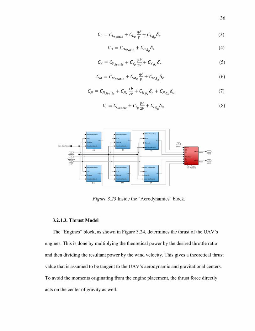
3.2.1.3. Thrust Model

The “Engines” block, as shown in Figure 3.24, determines the thrust of the UAV’s

engines. This is done by multiplying the theoretical power by the desired throttle ratio

and then dividing the resultant power by the wind velocity. This gives a theoretical thrust

value that is assumed to be tangent to the UAV’s aerodynamic and gravitational centers.

To avoid the moments originating from the engine placement, the thrust force directly

acts on the center of gravity as well.

37

Figure 3.24 Thrust model

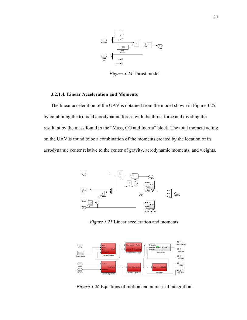
3.2.1.4. Linear Acceleration and Moments

The linear acceleration of the UAV is obtained from the model shown in Figure 3.25,

by combining the tri-axial aerodynamic forces with the thrust force and dividing the

resultant by the mass found in the “Mass, CG and Inertia” block. The total moment acting

on the UAV is found to be a combination of the moments created by the location of its

aerodynamic center relative to the center of gravity, aerodynamic moments, and weights.

Figure 3.25 Linear acceleration and moments.

Figure 3.26 Equations of motion and numerical integration.

38

3.2.1.5. Equations of Motion and Numerical Integration

The “Equations of Motion and Numerical Integration” block as shown in Figure 3.26

computes the position, orientation, and linear & angular velocities of the UAV.

Additionally, this block integrates the wind shear model defined in the standard

atmosphere section by adding the resultant wind speed to the linear velocity.

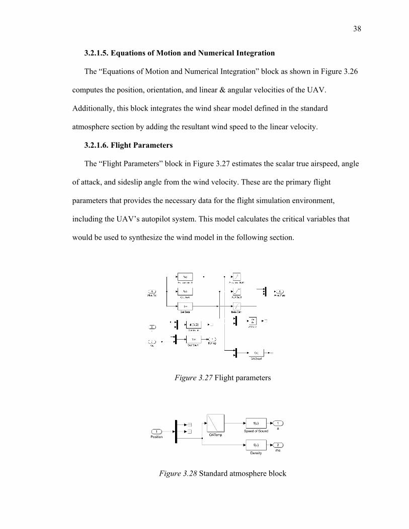
3.2.1.6. Flight Parameters

The “Flight Parameters” block in Figure 3.27 estimates the scalar true airspeed, angle

of attack, and sideslip angle from the wind velocity. These are the primary flight

parameters that provides the necessary data for the flight simulation environment,

including the UAV’s autopilot system. This model calculates the critical variables that

would be used to synthesize the wind model in the following section.

Figure 3.27 Flight parameters

Figure 3.28 Standard atmosphere block

39

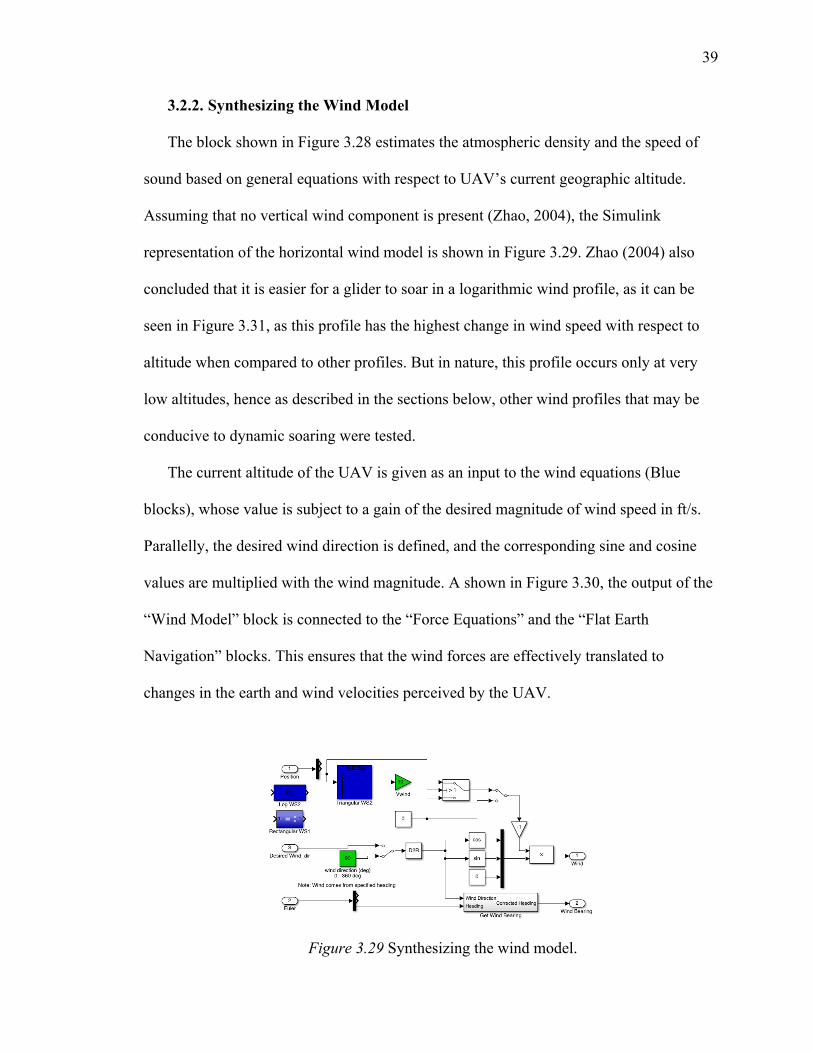
3.2.2. Synthesizing the Wind Model

The block shown in Figure 3.28 estimates the atmospheric density and the speed of

sound based on general equations with respect to UAV’s current geographic altitude.

Assuming that no vertical wind component is present (Zhao, 2004), the Simulink

representation of the horizontal wind model is shown in Figure 3.29. Zhao (2004) also

concluded that it is easier for a glider to soar in a logarithmic wind profile, as it can be

seen in Figure 3.31, as this profile has the highest change in wind speed with respect to

altitude when compared to other profiles. But in nature, this profile occurs only at very

low altitudes, hence as described in the sections below, other wind profiles that may be

conducive to dynamic soaring were tested.

The current altitude of the UAV is given as an input to the wind equations (Blue

blocks), whose value is subject to a gain of the desired magnitude of wind speed in ft/s.

Parallelly, the desired wind direction is defined, and the corresponding sine and cosine

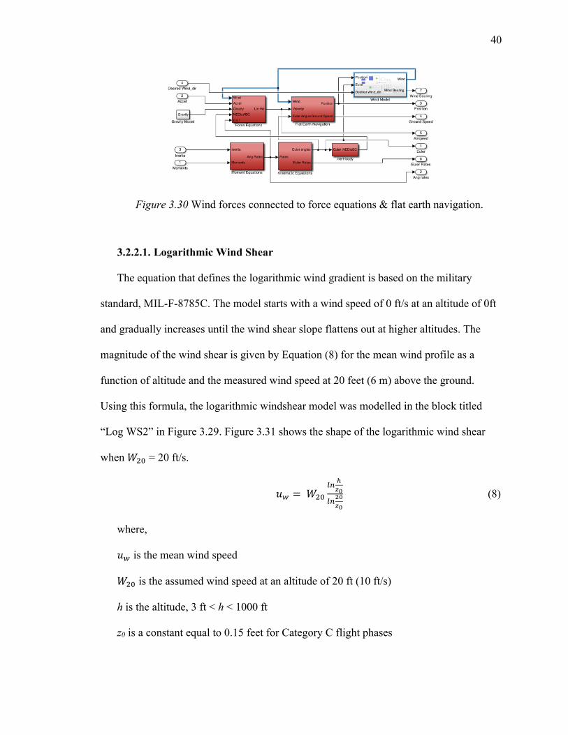
values are multiplied with the wind magnitude. A shown in Figure 3.30, the output of the

“Wind Model” block is connected to the “Force Equations” and the “Flat Earth

Navigation” blocks. This ensures that the wind forces are effectively translated to

changes in the earth and wind velocities perceived by the UAV.

Figure 3.29 Synthesizing the wind model.

40

Figure 3.30 Wind forces connected to force equations & flat earth navigation.

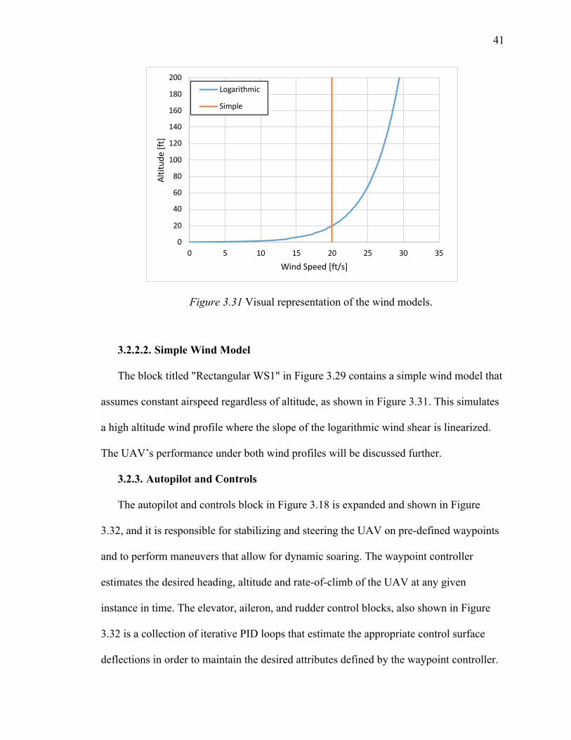
3.2.2.1. Logarithmic Wind Shear

The equation that defines the logarithmic wind gradient is based on the military

standard, MIL-F-8785C. The model starts with a wind speed of 0 ft/s at an altitude of 0ft

and gradually increases until the wind shear slope flattens out at higher altitudes. The

magnitude of the wind shear is given by Equation (8) for the mean wind profile as a

function of altitude and the measured wind speed at 20 feet (6 m) above the ground.

Using this formula, the logarithmic windshear model was modelled in the block titled

“Log WS2” in Figure 3.29. Figure 3.31 shows the shape of the logarithmic wind shear

when /01 = 20 ft/s.

./ =/01(; 456

(;'656 (8)

where,

./ is the mean wind speed

/01 is the assumed wind speed at an altitude of 20 ft (10 ft/s)

h is the altitude, 3 ft < h < 1000 ft

z0 is a constant equal to 0.15 feet for Category C flight phases

41

Figure 3.31 Visual representation of the wind models.

3.2.2.2. Simple Wind Model

The block titled "Rectangular WS1" in Figure 3.29 contains a simple wind model that

assumes constant airspeed regardless of altitude, as shown in Figure 3.31. This simulates

a high altitude wind profile where the slope of the logarithmic wind shear is linearized.

The UAV’s performance under both wind profiles will be discussed further.

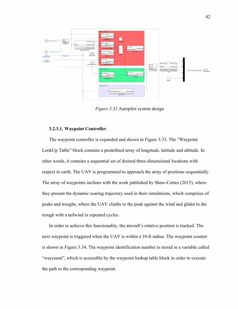
3.2.3. Autopilot and Controls

The autopilot and controls block in Figure 3.18 is expanded and shown in Figure

3.32, and it is responsible for stabilizing and steering the UAV on pre-defined waypoints

and to perform maneuvers that allow for dynamic soaring. The waypoint controller

estimates the desired heading, altitude and rate-of-climb of the UAV at any given

instance in time. The elevator, aileron, and rudder control blocks, also shown in Figure

3.32 is a collection of iterative PID loops that estimate the appropriate control surface

deflections in order to maintain the desired attributes defined by the waypoint controller.

0

20

40

60

80

100

120

140

160

180

200

0 5 10 15 20 25 30 35

Altit

ude

[ft]

Wind Speed [ft/s]

Logarithmic

Simple

42

Figure 3.32 Autopilot system design

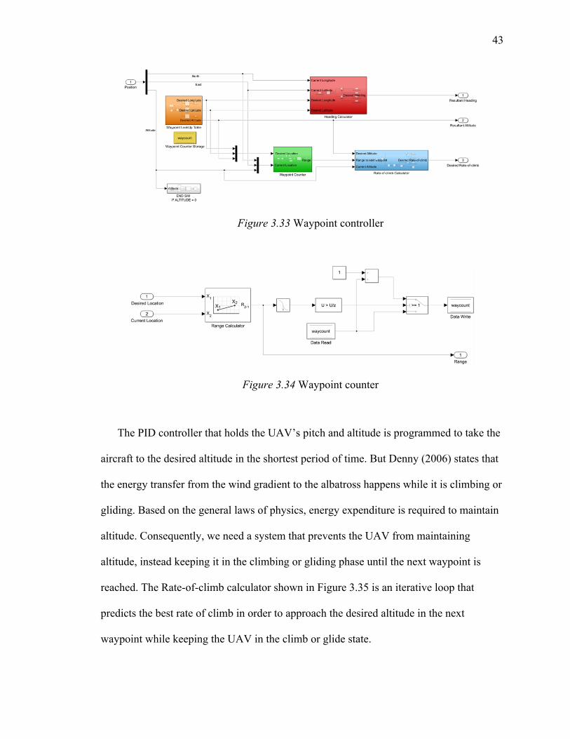
3.2.3.1. Waypoint Controller

The waypoint controller is expanded and shown in Figure 3.33. The “Waypoint

LookUp Table” block contains a predefined array of longitude, latitude and altitude. In

other words, it contains a sequential set of desired three-dimensional locations with

respect to earth. The UAV is programmed to approach the array of positions sequentially.

The array of waypoints inclines with the work published by Shaw-Cortez (2015), where

they present the dynamic soaring trajectory used in their simulations, which comprises of

peaks and troughs, where the UAV climbs to the peak against the wind and glides to the

trough with a tailwind in repeated cycles.

In order to achieve this functionality, the aircraft’s relative position is tracked. The

next waypoint is triggered when the UAV is within a 10-ft radius. The waypoint counter

is shown in Figure 3.34. The waypoint identification number is stored in a variable called

“waycount”, which is accessible by the waypoint lookup table block in order to execute

the path to the corresponding waypoint.

43

Figure 3.33 Waypoint controller

Figure 3.34 Waypoint counter

The PID controller that holds the UAV’s pitch and altitude is programmed to take the

aircraft to the desired altitude in the shortest period of time. But Denny (2006) states that

the energy transfer from the wind gradient to the albatross happens while it is climbing or

gliding. Based on the general laws of physics, energy expenditure is required to maintain

altitude. Consequently, we need a system that prevents the UAV from maintaining

altitude, instead keeping it in the climbing or gliding phase until the next waypoint is

reached. The Rate-of-climb calculator shown in Figure 3.35 is an iterative loop that

predicts the best rate of climb in order to approach the desired altitude in the next

waypoint while keeping the UAV in the climb or glide state.

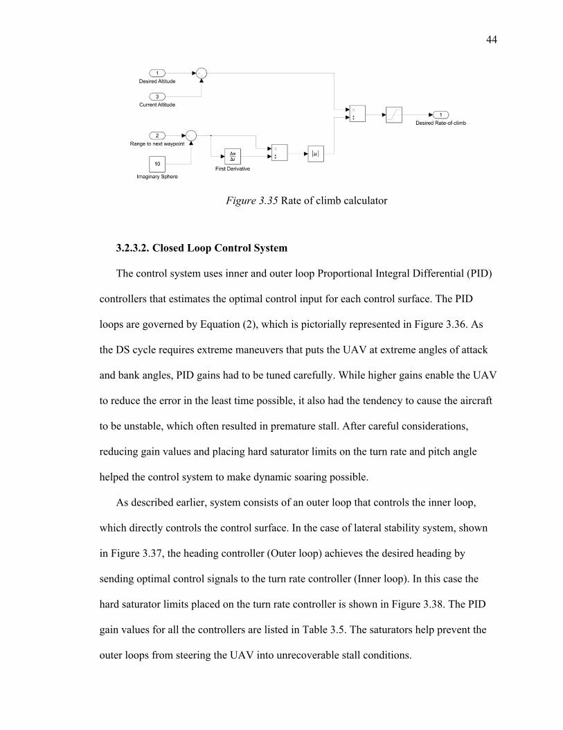
44

Figure 3.35 Rate of climb calculator

3.2.3.2. Closed Loop Control System

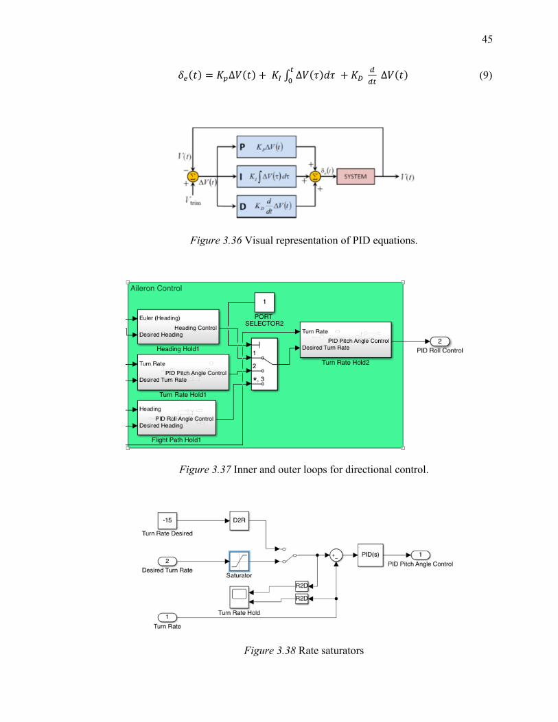
The control system uses inner and outer loop Proportional Integral Differential (PID)

controllers that estimates the optimal control input for each control surface. The PID

loops are governed by Equation (2), which is pictorially represented in Figure 3.36. As

the DS cycle requires extreme maneuvers that puts the UAV at extreme angles of attack

and bank angles, PID gains had to be tuned carefully. While higher gains enable the UAV

to reduce the error in the least time possible, it also had the tendency to cause the aircraft

to be unstable, which often resulted in premature stall. After careful considerations,

reducing gain values and placing hard saturator limits on the turn rate and pitch angle

helped the control system to make dynamic soaring possible.

As described earlier, system consists of an outer loop that controls the inner loop,

which directly controls the control surface. In the case of lateral stability system, shown

in Figure 3.37, the heading controller (Outer loop) achieves the desired heading by

sending optimal control signals to the turn rate controller (Inner loop). In this case the

hard saturator limits placed on the turn rate controller is shown in Figure 3.38. The PID

gain values for all the controllers are listed in Table 3.5. The saturators help prevent the

outer loops from steering the UAV into unrecoverable stall conditions.

45

*!(D) = E9∆G(D) +E< ∫ ∆G(I)JI=1 + E$

22= ∆G(D) (9)

Figure 3.36 Visual representation of PID equations.

Figure 3.37 Inner and outer loops for directional control.

Figure 3.38 Rate saturators

46

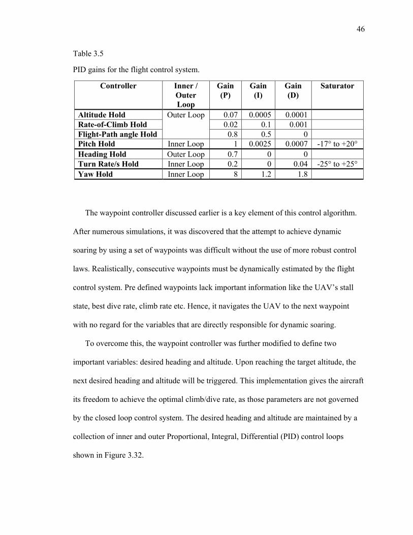
Table 3.5

PID gains for the flight control system.

Controller Inner / Outer Loop

Gain (P)

Gain (I)

Gain (D)

Saturator

Altitude Hold Outer Loop 0.07 0.0005 0.0001 Rate-of-Climb Hold 0.02 0.1 0.001 Flight-Path angle Hold 0.8 0.5 0 Pitch Hold Inner Loop 1 0.0025 0.0007 -17° to +20° Heading Hold Outer Loop 0.7 0 0 Turn Rate/s Hold Inner Loop 0.2 0 0.04 -25° to +25° Yaw Hold Inner Loop 8 1.2 1.8

The waypoint controller discussed earlier is a key element of this control algorithm.

After numerous simulations, it was discovered that the attempt to achieve dynamic

soaring by using a set of waypoints was difficult without the use of more robust control

laws. Realistically, consecutive waypoints must be dynamically estimated by the flight

control system. Pre defined waypoints lack important information like the UAV’s stall

state, best dive rate, climb rate etc. Hence, it navigates the UAV to the next waypoint

with no regard for the variables that are directly responsible for dynamic soaring.

To overcome this, the waypoint controller was further modified to define two

important variables: desired heading and altitude. Upon reaching the target altitude, the

next desired heading and altitude will be triggered. This implementation gives the aircraft

its freedom to achieve the optimal climb/dive rate, as those parameters are not governed

by the closed loop control system. The desired heading and altitude are maintained by a

collection of inner and outer Proportional, Integral, Differential (PID) control loops

shown in Figure 3.32.

47

The inner loop reduces the error in the aircraft’s orientation in space by directly

sending control inputs to the corresponding control surfaces. Simultaneously, the outer

loop reduces the aircraft’s positional error by controlling the inner loop. The error here, is

defined as the difference between the current and desired position. This controls bus is

sent back into the aircraft dynamics model in Figure 3.19, hence making this a closed-

loop flight simulation environment.

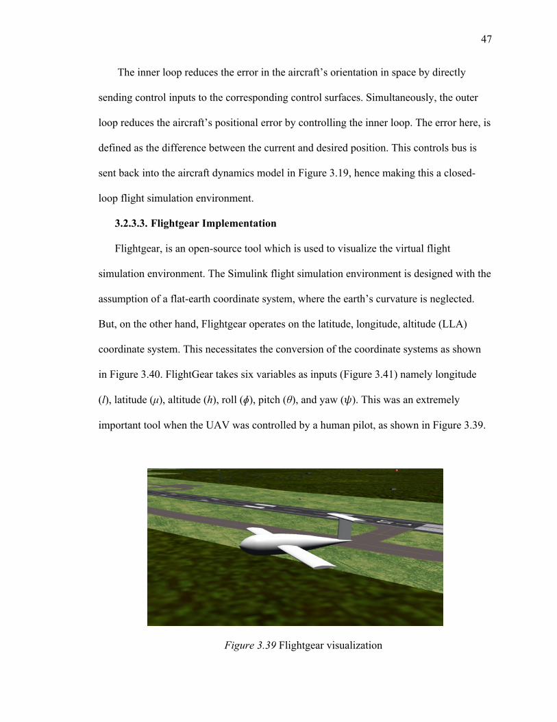
3.2.3.3. Flightgear Implementation

Flightgear, is an open-source tool which is used to visualize the virtual flight

simulation environment. The Simulink flight simulation environment is designed with the

assumption of a flat-earth coordinate system, where the earth’s curvature is neglected.

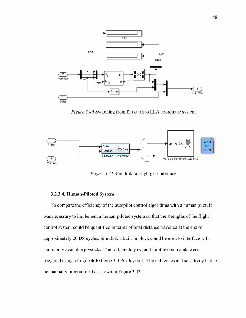
But, on the other hand, Flightgear operates on the latitude, longitude, altitude (LLA)

coordinate system. This necessitates the conversion of the coordinate systems as shown

in Figure 3.40. FlightGear takes six variables as inputs (Figure 3.41) namely longitude

(l), latitude (μ), altitude (h), roll (ɸ), pitch (θ), and yaw (K). This was an extremely

important tool when the UAV was controlled by a human pilot, as shown in Figure 3.39.

Figure 3.39 Flightgear visualization

48

Figure 3.40 Switching from flat earth to LLA coordinate system.

Figure 3.41 Simulink to Flightgear interface.

3.2.3.4. Human-Piloted System

To compare the efficiency of the autopilot control algorithms with a human pilot, it

was necessary to implement a human-piloted system so that the strengths of the flight

control system could be quantified in terms of total distance travelled at the end of

approximately 20 DS cycles. Simulink’s built-in block could be used to interface with

commonly available joysticks. The roll, pitch, yaw, and throttle commands were

triggered using a Logitech Extreme 3D Pro Joystick. The null zones and sensitivity had to

be manually programmed as shown in Figure 3.42.

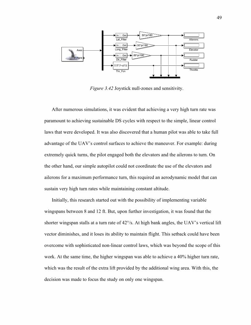
49

Figure 3.42 Joystick null-zones and sensitivity.

After numerous simulations, it was evident that achieving a very high turn rate was

paramount to achieving sustainable DS cycles with respect to the simple, linear control

laws that were developed. It was also discovered that a human pilot was able to take full

advantage of the UAV’s control surfaces to achieve the maneuver. For example: during

extremely quick turns, the pilot engaged both the elevators and the ailerons to turn. On

the other hand, our simple autopilot could not coordinate the use of the elevators and

ailerons for a maximum performance turn, this required an aerodynamic model that can

sustain very high turn rates while maintaining constant altitude.

Initially, this research started out with the possibility of implementing variable

wingspans between 8 and 12 ft. But, upon further investigation, it was found that the

shorter wingspan stalls at a turn rate of 42°/s. At high bank angles, the UAV’s vertical lift

vector diminishes, and it loses its ability to maintain flight. This setback could have been

overcome with sophisticated non-linear control laws, which was beyond the scope of this

work. At the same time, the higher wingspan was able to achieve a 40% higher turn rate,

which was the result of the extra lift provided by the additional wing area. With this, the

decision was made to focus the study on only one wingspan.

50

3.3. Modifying the Aerodynamic Model

Some drawbacks of the initial aircraft geometry led to the modification of the

aerodynamic model, as the repeatable dynamic soaring cycles were contingent upon this.

The methodology to capture the aerodynamic characteristics of a small UAV using

variable-fidelity analysis on ANSYS Fluent (High fidelity tool) and SURFACES (Low

fidelity tool) which was presented earlier.

The initial configuration, shown in Figure 3.2, was developed as a simple baseline

configuration that would be easily replicated by future researchers. The introduction of

the resulting aerodynamic model into the flight simulation environment revealed the

configuration was too aerodynamically inefficient to sustain dynamic soaring. The

principal drawback being its less-than-optimal lift to drag ratio of 10. In contrast, the

albatross achieves DS with a L/D ratio as high as 25 (Denny, 2006). Furthermore, the

albatross can also morph its body in order to better adapt to each phase of the DS

maneuver. While extreme vehicle morphing can be simulated theoretically, it is a

prohibitively challenging engineering problem to construct a morphing UAV.

As it can be seen later, the resulting aerodynamic model permits human and

automated sustenance of DS. The revised model utilizes a planform geometry based on

the wing of the albatross (Stempeck, 2018). The new geometry was initially designed

with a T-tail, which resulted in values of the Cnb, Clb, and Clr derivatives that made

lateral/directional handling of the aircraft unacceptable. This was remedied by switching

to a conventional tail and by reducing Clb by maintaining the outboard anhedral of the

albatross planform geometry. These changes substantially improved the Dutch roll

damping of the model, permitting easier and more responsive flight dynamics.

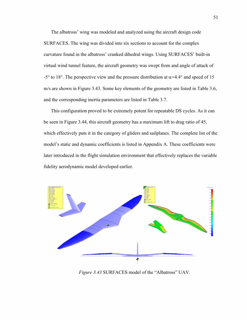
51

The albatross’ wing was modeled and analyzed using the aircraft design code

SURFACES. The wing was divided into six sections to account for the complex

curvature found in the albatross’ cranked dihedral wings. Using SURFACES’ built-in

virtual wind tunnel feature, the aircraft geometry was swept from and angle of attack of

-5° to 18°. The perspective view and the pressure distribution at a=4.4° and speed of 15

m/s are shown in Figure 3.43. Some key elements of the geometry are listed in Table 3.6,

and the corresponding inertia parameters are listed in Table 3.7.

This configuration proved to be extremely potent for repeatable DS cycles. As it can

be seen in Figure 3.44, this aircraft geometry has a maximum lift to drag ratio of 45,

which effectively puts it in the category of gliders and sailplanes. The complete list of the

model’s static and dynamic coefficients is listed in Appendix A. These coefficients were

later introduced in the flight simulation environment that effectively replaces the variable

fidelity aerodynamic model developed earlier.

Figure 3.43 SURFACES model of the “Albatross” UAV.

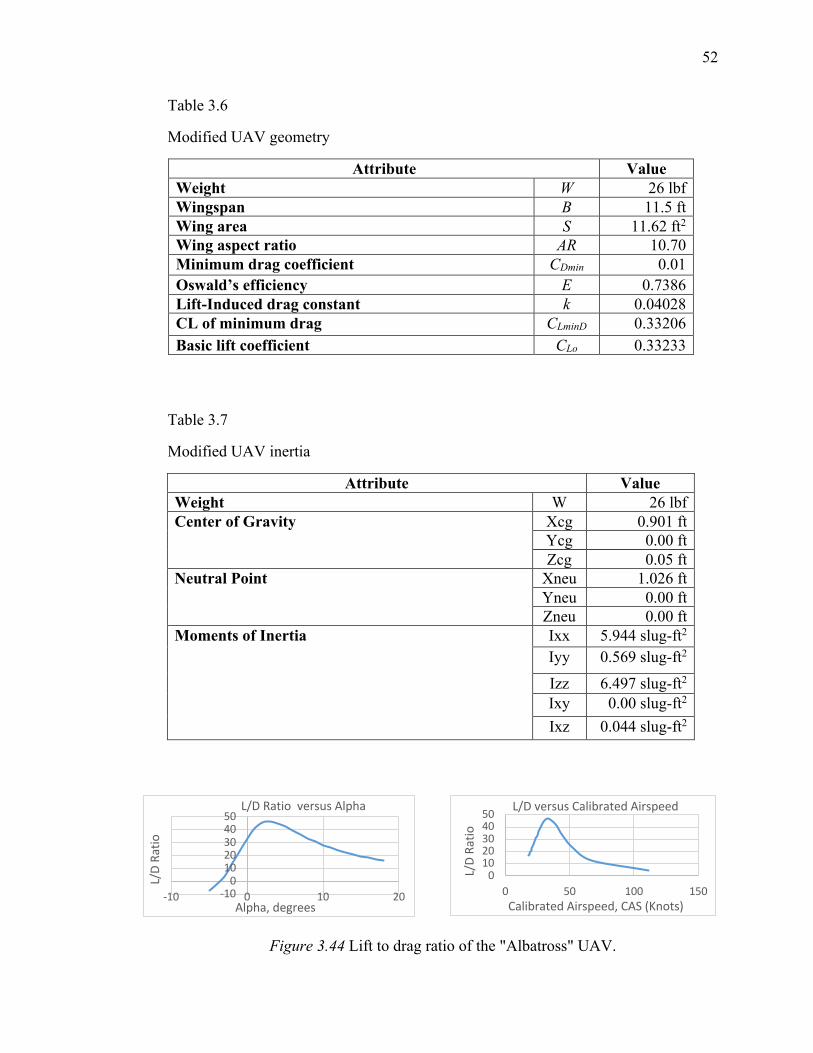
52

Table 3.6

Modified UAV geometry

Attribute Value Weight W 26 lbf Wingspan B 11.5 ft Wing area S 11.62 ft2 Wing aspect ratio AR 10.70 Minimum drag coefficient CDmin 0.01 Oswald’s efficiency E 0.7386 Lift-Induced drag constant k 0.04028 CL of minimum drag CLminD 0.33206 Basic lift coefficient CLo 0.33233

Table 3.7

Modified UAV inertia

Attribute Value Weight W 26 lbf Center of Gravity Xcg 0.901 ft

Ycg 0.00 ft Zcg 0.05 ft

Neutral Point Xneu 1.026 ft Yneu 0.00 ft Zneu 0.00 ft

Moments of Inertia Ixx 5.944 slug-ft2 Iyy 0.569 slug-ft2 Izz 6.497 slug-ft2 Ixy 0.00 slug-ft2 Ixz 0.044 slug-ft2

Figure 3.44 Lift to drag ratio of the "Albatross" UAV.

-1001020304050

-10 0 10 20

L/D

Ratio

Alpha, degrees

L/D Ratio versus Alpha

01020304050

0 50 100 150

L/D

Ratio

Calibrated Airspeed, CAS (Knots)

L/D versus Calibrated Airspeed

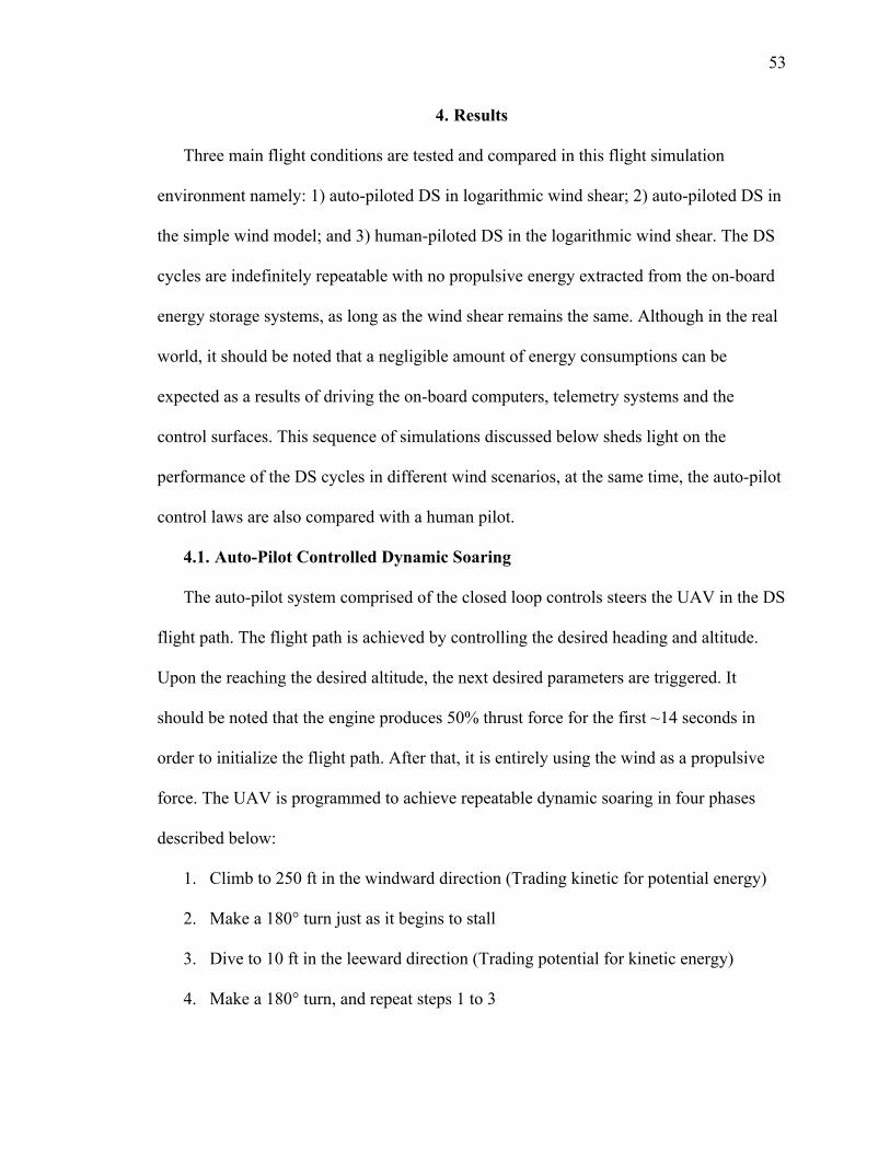
53

4. Results

Three main flight conditions are tested and compared in this flight simulation

environment namely: 1) auto-piloted DS in logarithmic wind shear; 2) auto-piloted DS in

the simple wind model; and 3) human-piloted DS in the logarithmic wind shear. The DS

cycles are indefinitely repeatable with no propulsive energy extracted from the on-board

energy storage systems, as long as the wind shear remains the same. Although in the real

world, it should be noted that a negligible amount of energy consumptions can be

expected as a results of driving the on-board computers, telemetry systems and the

control surfaces. This sequence of simulations discussed below sheds light on the

performance of the DS cycles in different wind scenarios, at the same time, the auto-pilot

control laws are also compared with a human pilot.

4.1. Auto-Pilot Controlled Dynamic Soaring

The auto-pilot system comprised of the closed loop controls steers the UAV in the DS

flight path. The flight path is achieved by controlling the desired heading and altitude.

Upon the reaching the desired altitude, the next desired parameters are triggered. It

should be noted that the engine produces 50% thrust force for the first ~14 seconds in

order to initialize the flight path. After that, it is entirely using the wind as a propulsive

force. The UAV is programmed to achieve repeatable dynamic soaring in four phases

described below:

1. Climb to 250 ft in the windward direction (Trading kinetic for potential energy)

2. Make a 180° turn just as it begins to stall

3. Dive to 10 ft in the leeward direction (Trading potential for kinetic energy)

4. Make a 180° turn, and repeat steps 1 to 3

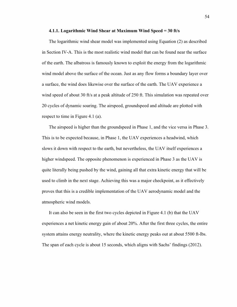
54

4.1.1. Logarithmic Wind Shear at Maximum Wind Speed = 30 ft/s

The logarithmic wind shear model was implemented using Equation (2) as described

in Section IV-A. This is the most realistic wind model that can be found near the surface

of the earth. The albatross is famously known to exploit the energy from the logarithmic

wind model above the surface of the ocean. Just as any flow forms a boundary layer over

a surface, the wind does likewise over the surface of the earth. The UAV experience a

wind speed of about 30 ft/s at a peak altitude of 250 ft. This simulation was repeated over

20 cycles of dynamic soaring. The airspeed, groundspeed and altitude are plotted with

respect to time in Figure 4.1 (a).

The airspeed is higher than the groundspeed in Phase 1, and the vice versa in Phase 3.

This is to be expected because, in Phase 1, the UAV experiences a headwind, which

slows it down with respect to the earth, but nevertheless, the UAV itself experiences a

higher windspeed. The opposite phenomenon is experienced in Phase 3 as the UAV is

quite literally being pushed by the wind, gaining all that extra kinetic energy that will be

used to climb in the next stage. Achieving this was a major checkpoint, as it effectively

proves that this is a credible implementation of the UAV aerodynamic model and the

atmospheric wind models.

It can also be seen in the first two cycles depicted in Figure 4.1 (b) that the UAV

experiences a net kinetic energy gain of about 20%. After the first three cycles, the entire

system attains energy neutrality, where the kinetic energy peaks out at about 5500 ft-lbs.

The span of each cycle is about 15 seconds, which aligns with Sachs’ findings (2012).

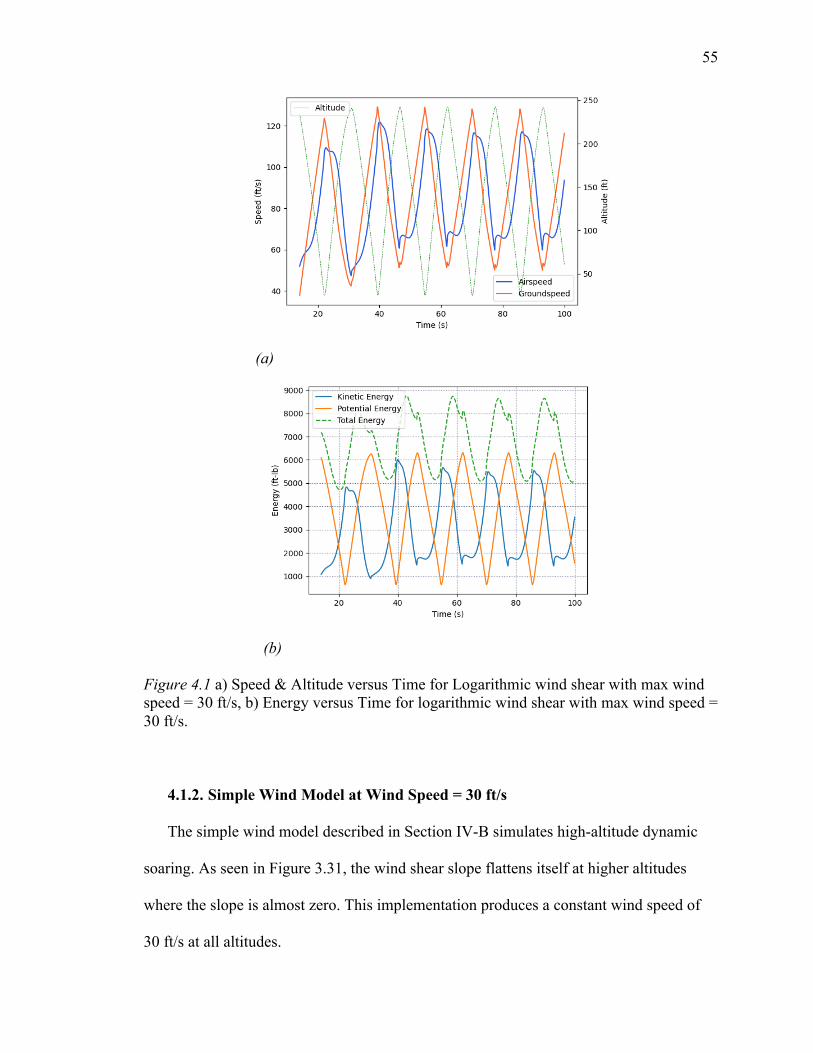
55

(a)

(b)

Figure 4.1 a) Speed & Altitude versus Time for Logarithmic wind shear with max wind speed = 30 ft/s, b) Energy versus Time for logarithmic wind shear with max wind speed = 30 ft/s.

4.1.2. Simple Wind Model at Wind Speed = 30 ft/s

The simple wind model described in Section IV-B simulates high-altitude dynamic

soaring. As seen in Figure 3.31, the wind shear slope flattens itself at higher altitudes

where the slope is almost zero. This implementation produces a constant wind speed of

30 ft/s at all altitudes.

56

The speed and altitude are plotted with respect to time in Figure 4.2 (a). Overall, the

curves follow the same pattern as the logarithmic wind model; however, there are a few

differences that can be noticed. The airspeed range is wider in the logarithmic wind shear

as compared to the simple wind model. This phenomenon can be directly traced back to

the fact that the logarithmic model has an extremely wide range of wind speeds with

respect to altitude. The same pattern can be observed in Figure 4.2 (b) as well, where the

kinetic energy fluctuates less, as compared to the logarithmic wind model.

The maximum kinetic energy in the simple wind model is about 9 % lesser than that

of the logarithmic model. This indicates that the UAV is not utilizing all its potential

energy, where excess energy goes unused. This could be made even better by increasing

the altitude delta in the DS cycle. Nevertheless, this research also shows that dynamic

soaring is possible at higher altitudes.

4.1.3. Total Distance Travelled

Interestingly, the simple wind model, which represents high-altitude dynamic soaring,

the UAV travels a slightly higher distance of ~700 ft over 20 cycles when compared to

the logarithmic wind model, as shown in Figure 4.5, which is about 11% higher. For

comparison, the albatross flies thousands of miles per day, where the small increments in

the distance gained could results in a significant amount over thousands of repeated DS

cycles. It should also be noted that the wind is blowing from the positive side of the

“East” axis. With respect to the wind direction, the UAV is performing repeated cycles of

climbing and diving.

57

(a)

(b)

Figure 4.2 a) Speed & Altitude versus Time for simple wind model with max wind speed = 30 ft/s, b) Energy versus Time for simple wind model with max wind speed = 30 ft/s.

An interesting observation from Figure 4.4 is that the logarithmic wind model keeps

the UAV travelling in a direction that is almost perpendicular to the wind direction. The

entire DS flight path is shown in Figure 4.3. At the same time, the simple wind model

gradually pushes the UAV off course, where the UAV may not have enough freedom to

steer itself in the desired direction.

58

With any flight mission, the UAV must travel from point A to B. In dynamic soaring,

it may not arrive at point B in the most direct path, but it must arrive at point B,

nevertheless. Hence, the freedom to change course at the macro level is key to make way

for real-world applications. It can be concluded that some directional controllability may

be lost with the simple wind model.

Figure 4.3 Auto-piloted dynamic soaring flight path.

Figure 4.4 Auto-piloted dynamic soaring flight path (First three cycles).

59

Figure 4.5 Total distance travelled by the auto-piloted UAV in approximately 20 dynamic soaring cycles.

4.1.4. Minimum Wind Shear Required

As shown in Figure 4.6, below a certain minimum magnitude of wind speed, the

UAV experiences a net energy loss at the end of each cycle, which eventually results in a

stall. After numerous simulations, it was estimated that the absolute minimum wind shear

required to achieve DS is 28.8 ft/s at peak altitude for the logarithmic model. This results

in a wind speed of 19 ft/s at an altitude of 20 ft in Equation (1).

Alternatively, the minimum wind speed required for the simple wind model is 26 ft/s,

which is only slightly lagging the logarithmic model. Keeping in mind that the simple

model has a constant wind speed with respect to altitude, while the logarithmic model has

a very low wind speed at altitudes very close to the ground. Despite this, the minimum

required wind shear for both models is very close. This shows that the UAV can extract

maximum energy from the logarithmic model.

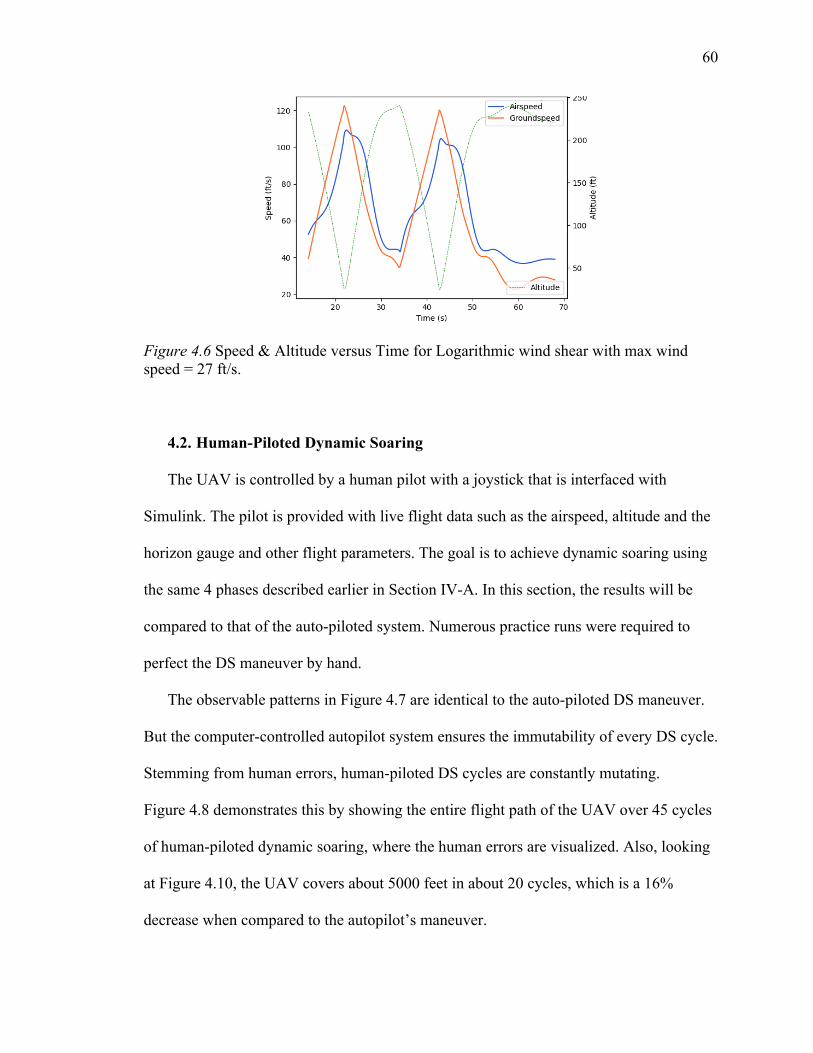
60

Figure 4.6 Speed & Altitude versus Time for Logarithmic wind shear with max wind speed = 27 ft/s.

4.2. Human-Piloted Dynamic Soaring

The UAV is controlled by a human pilot with a joystick that is interfaced with

Simulink. The pilot is provided with live flight data such as the airspeed, altitude and the

horizon gauge and other flight parameters. The goal is to achieve dynamic soaring using

the same 4 phases described earlier in Section IV-A. In this section, the results will be

compared to that of the auto-piloted system. Numerous practice runs were required to

perfect the DS maneuver by hand.

The observable patterns in Figure 4.7 are identical to the auto-piloted DS maneuver.

But the computer-controlled autopilot system ensures the immutability of every DS cycle.

Stemming from human errors, human-piloted DS cycles are constantly mutating.

Figure 4.8 demonstrates this by showing the entire flight path of the UAV over 45 cycles

of human-piloted dynamic soaring, where the human errors are visualized. Also, looking

at Figure 4.10, the UAV covers about 5000 feet in about 20 cycles, which is a 16%

decrease when compared to the autopilot’s maneuver.

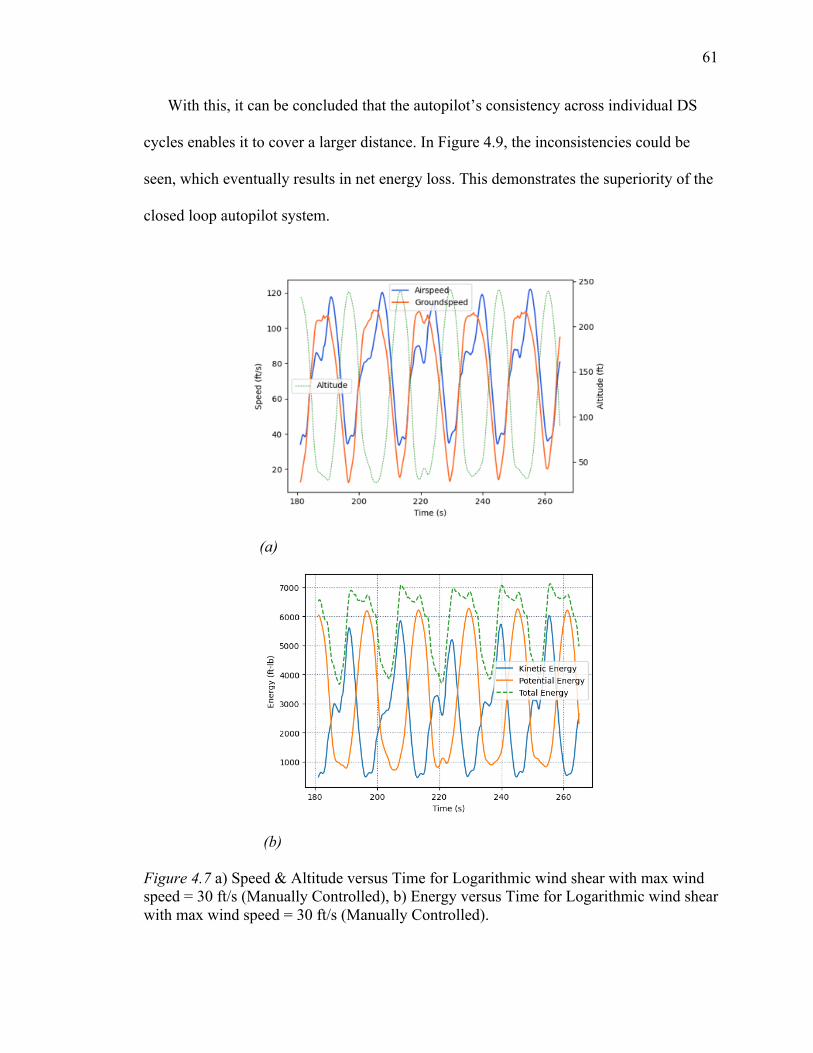
61

With this, it can be concluded that the autopilot’s consistency across individual DS

cycles enables it to cover a larger distance. In Figure 4.9, the inconsistencies could be

seen, which eventually results in net energy loss. This demonstrates the superiority of the

closed loop autopilot system.

(a)

(b)

Figure 4.7 a) Speed & Altitude versus Time for Logarithmic wind shear with max wind speed = 30 ft/s (Manually Controlled), b) Energy versus Time for Logarithmic wind shear with max wind speed = 30 ft/s (Manually Controlled).

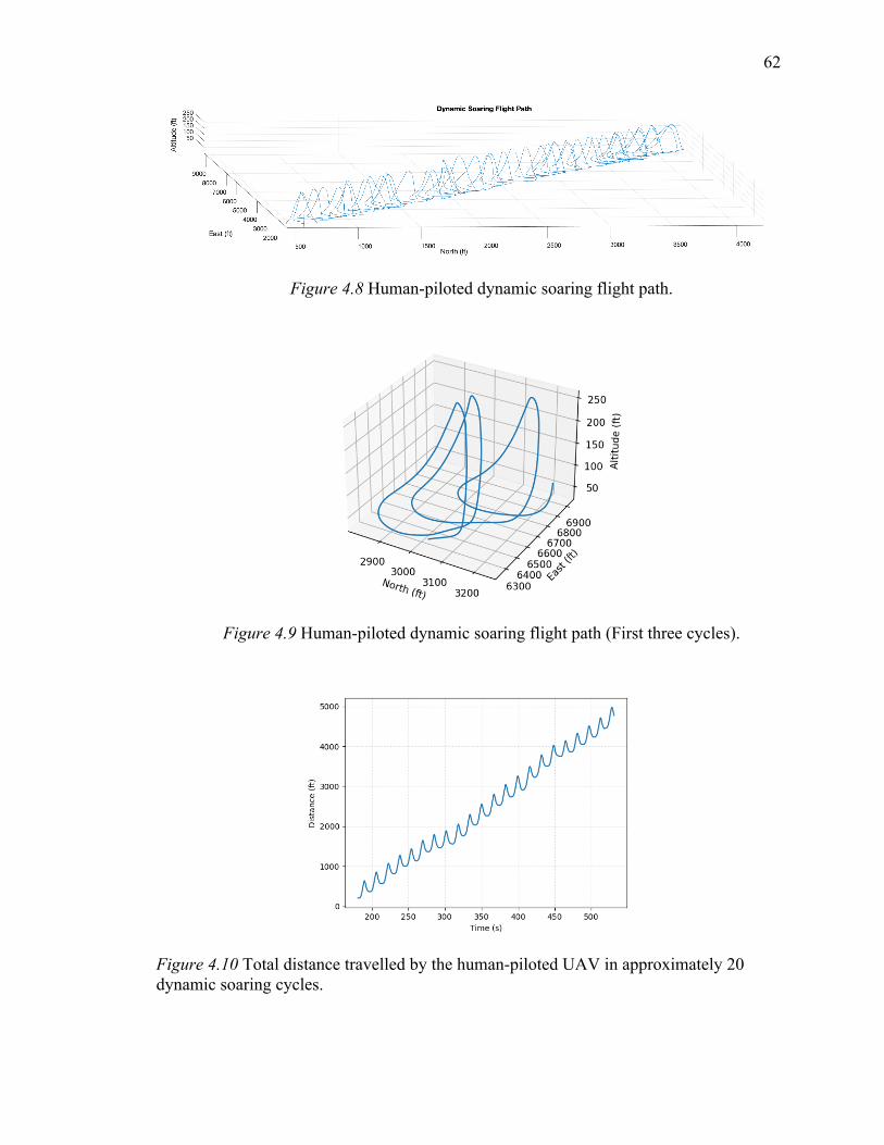
62

Figure 4.8 Human-piloted dynamic soaring flight path.

Figure 4.9 Human-piloted dynamic soaring flight path (First three cycles).

Figure 4.10 Total distance travelled by the human-piloted UAV in approximately 20 dynamic soaring cycles.

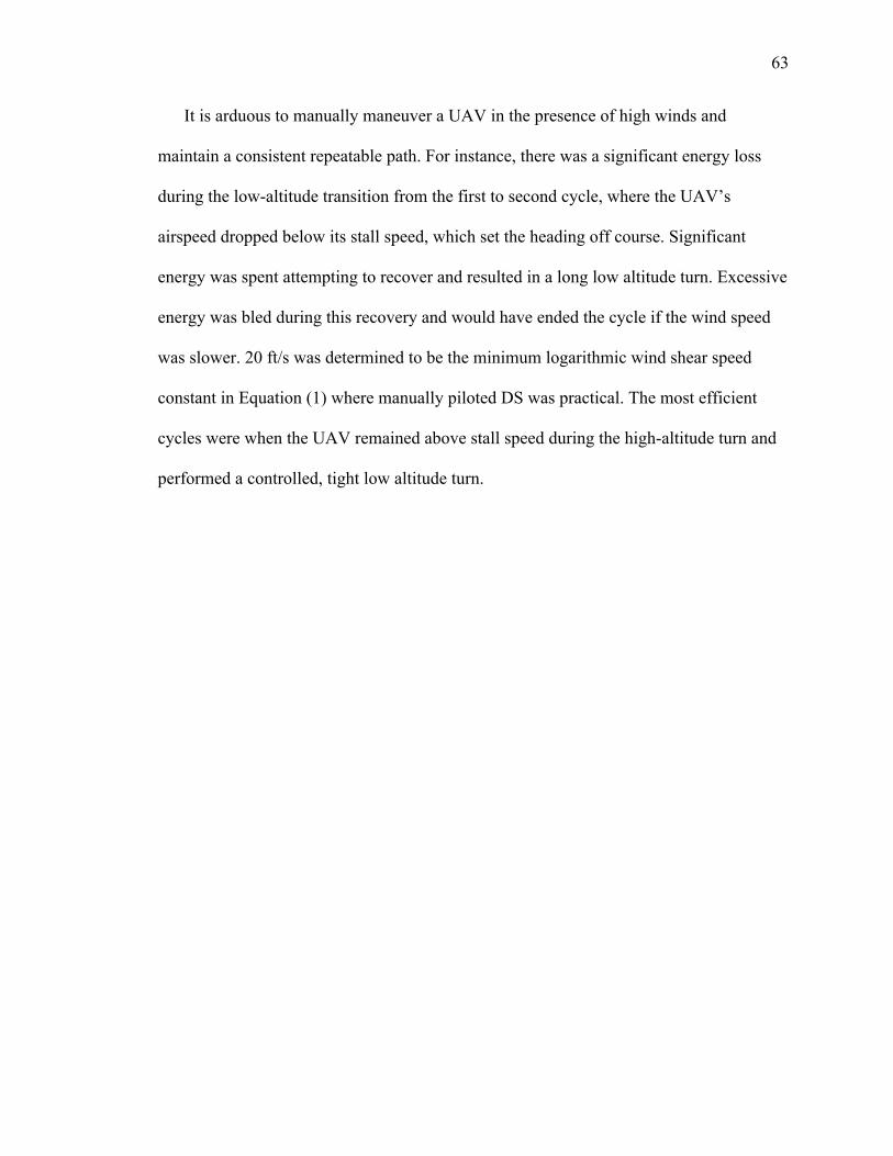
63

It is arduous to manually maneuver a UAV in the presence of high winds and

maintain a consistent repeatable path. For instance, there was a significant energy loss

during the low-altitude transition from the first to second cycle, where the UAV’s

airspeed dropped below its stall speed, which set the heading off course. Significant

energy was spent attempting to recover and resulted in a long low altitude turn. Excessive

energy was bled during this recovery and would have ended the cycle if the wind speed

was slower. 20 ft/s was determined to be the minimum logarithmic wind shear speed

constant in Equation (1) where manually piloted DS was practical. The most efficient

cycles were when the UAV remained above stall speed during the high-altitude turn and

performed a controlled, tight low altitude turn.

64

5. Discussions, Conclusions, and Recommendations

The aerodynamic model, auto-pilot control laws, a 6DoF flight simulation

environment, and a simple dynamic soaring algorithm was successfully developed from

scratch. At the outset, this project presents a paradigm shift in UAV propulsion, resulting

in a significant reduction in energy expenditure when the flight pattern of the albatross is

implemented on man-made aircrafts.

5.1. Discussions

The two major components of this work are described below. These components of

the flight simulation environment constitute the elementary building blocks of the flight

simulation environment, which was built using MATLAB and Simulink as a platform.

This also depicts a credible way to capture the aerodynamic model of an aircraft model

for the purpose of testing on a virtual environment.

5.1.1. Hybrid Aerodynamic Model

A variable-fidelity approach to predict aerodynamic and aircraft stability

characteristics of an aircraft model with morphing wing technology designed for the

dynamic-soaring (DS) flightpath was implemented and validated against available

experimental data. The low-fidelity tool based on the potential flow solver is highly

efficient but must be supplemented with high-fidelity viscous flow solutions to predict

the aircraft parameters at the critical stages of the dynamic-soaring trajectory

characterized by near-stall flow regimes. Preliminary results of the flight-path analysis

conducted for selected stages of the DS trajectory revealed a significant impact of the

variable span on the aircraft aerodynamic performance.

65

5.1.2. 6DoF Flight Simulation Environment

The closed-loop flight simulation environment is designed and built on MATLAB &

Simulink, where the hybrid aerodynamic model successfully represents the UAV’s

aerodynamic behavior in simulated flight. In addition to this, a simple autopilot & flight

control system is designed and developed to enable the UAV to navigate the simulated

world in predefined paths, as defined by the waypoint controller. The modular approach

to design the aircraft dynamics model makes it conducive to use the same environment to

simulate other aircrafts or scenarios by substituting the blocks with your own. This

environment was used as a platform to study and quantify the net energy gain in

repeatable dynamic soaring. Also, the modularity of the flight simulation environment

ensures its reusability by future researchers who wish to carry on with this work.

5.2. Conclusions

The results presented in this work is highly dependent on three important factors,

which are: 1) the aircraft geometry; 2) control laws; and 3) wind shear model. A change

in any of these parameters could prove to be beneficial or detrimental to dynamic soaring.

The perpetual dynamic soaring maneuver has been successfully simulated on the virtual

simulation environment designed on MATLAB and Simulink. This work serves to be a

virtual representation of dynamic soaring where the groundwork for a potential real world

dynamic soaring UAV has been laid out. This also serves as a benchmark for the optimal

aerodynamic model and the prerequisites of the autopilot system are defined for dynamic

soaring to be conducive. After testing a variety of scenarios in the virtual simulation

environment, the most significant results from this work are listed below:

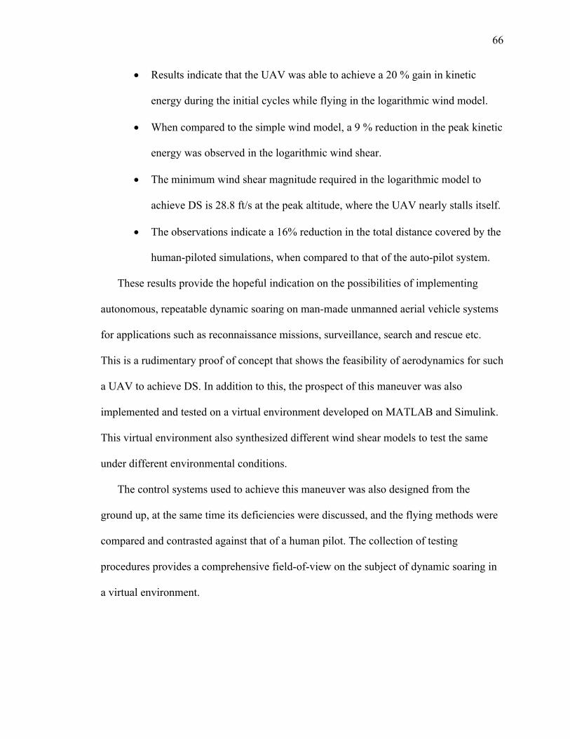
66

• Results indicate that the UAV was able to achieve a 20 % gain in kinetic

energy during the initial cycles while flying in the logarithmic wind model.

• When compared to the simple wind model, a 9 % reduction in the peak kinetic

energy was observed in the logarithmic wind shear.

• The minimum wind shear magnitude required in the logarithmic model to

achieve DS is 28.8 ft/s at the peak altitude, where the UAV nearly stalls itself.

• The observations indicate a 16% reduction in the total distance covered by the

human-piloted simulations, when compared to that of the auto-pilot system.

These results provide the hopeful indication on the possibilities of implementing

autonomous, repeatable dynamic soaring on man-made unmanned aerial vehicle systems

for applications such as reconnaissance missions, surveillance, search and rescue etc.

This is a rudimentary proof of concept that shows the feasibility of aerodynamics for such

a UAV to achieve DS. In addition to this, the prospect of this maneuver was also

implemented and tested on a virtual environment developed on MATLAB and Simulink.

This virtual environment also synthesized different wind shear models to test the same

under different environmental conditions.

The control systems used to achieve this maneuver was also designed from the

ground up, at the same time its deficiencies were discussed, and the flying methods were

compared and contrasted against that of a human pilot. The collection of testing

procedures provides a comprehensive field-of-view on the subject of dynamic soaring in

a virtual environment.

67

5.3. Recommendations

While the autopilot system is clearly superior to the human pilot, it was also observed

to be a bottleneck in this entire process as it lacked the ability to perform complex

maneuvers that could potentially result in a lower minimum required wind shear. This

comparison provides the rationale for the need to develop a sophisticated non-linear

autopilot control system that can maximize the net energy gained due to dynamic soaring.

As the scenarios described above are discussed for specific wind-shear conditions, the

need for implementing artificial intelligence for flight path estimation was realized. More

specifically, it was determined that unsupervised machine learning methodology known

as Reinforcement Learning was deemed to be the best methodology for this study. This

involves an agent (UAV) that can learn from its environment without the need for large,

complex data sets for training. Instead, the agent tries to perform actions for the purpose

of gaining rewards of variable weightage for different circumstances. This learning

paradigm would establish the best DS flight path under any environmental conditions.

This implementation is paramount to testing DS maneuvers in the real world due to the

volatility of atmospheric weather conditions.

This leads to the next important step in this research, where a real-world 3D model of

the UAV could be fabricated using the aerodynamic model discussed here, and the

control algorithms could be tested for their credibility. Nevertheless, this presents a

paradigm shift in UAV propulsion where the energy extracted from the atmospheric wind

shear can be used as a propulsive force.

68

REFERENCES

Barnes, J. P. (2004). How Flies the Albatross – the Flight Mechanics of Dynamic Soaring. SAE Technical Paper Series. https://doi.org/10.4271/2004-01-3088

Cone, C. D. (1964). A Mathematical Analysis of the Dynamic Soaring Flight of the

Albatross with Ecological Interpretations. Virginia Institute of Marine Science. Retrieved from https://scholarworks.wm.edu/reports/101/

Deittert, M., Richards, A., Toomer, C. A., & Pipe, A. (2009). Engineless Unmanned

Aerial Vehicle Propulsion by Dynamic Soaring. Journal of Guidance, Control, and Dynamics, 32(5), (pp. 1446–1457). doi: 10.2514/1.43270

Denny, M. (2008). Dynamic soaring: aerodynamics for albatrosses. European Journal of

Physics, 30(1), (pp. 75–84). doi: 10.1088/0143-0807/30/1/008 Gudmundsson, S. (2016). A biomimetic, energy-harvesting, obstacle-avoiding, path-

planning algorithm for UAVs. Embry-Riddle Aeronautical University. Retrieved from https://commons.erau.edu/cgi/viewcontent.cgi?article=1305&context=edt

Gudmundsson, S., Golubev, V., Drakunov, S., & Reinholtz, C. (2019). Bio-Inspired

Methodologies for Energy Conservation and Harvesting Flight-Path Modeling for Unmanned Aerial System. Journal of Aerospace Information Systems, 16(7), (pp. 289–295). doi: 10.2514/1.i010597

Pennycuick, C.J., The flight of petrels and albatrosses (procellariiformes), observed in

South Georgia and its vicinity. (1982). Philosophical Transactions of the Royal Society of London. B, Biological Sciences, 300(1098), (pp. 75–106). doi: 10.1098/rstb.1982.0158

Peyret, R., & Egon Krause. (2000). Advanced turbulent flow computations. Wien ; New

York: Springer, Cop. Rayleigh. (1883). The Soaring of Birds. Nature, 27(701), (pp. 534–535).

doi: 10.1038/027534a0 Sachs, G. P. (2019). Dynamic Soaring at 600 mph. AIAA Scitech 2019 Forum.

doi: 10.2514/6.2019-0107 Sachs, G. P. (2020). Optimal Acceleration Procedure from Launch to Maximum Speed in

High-Speed Dynamic Soaring. AIAA Scitech 2020 Forum. doi: 10.2514/6.2020-0024

69

Sachs, G., Traugott, J., Nesterova, A. P., Dell’Omo, G., Kümmeth, F., Heidrich, W., Vyssotski, A. L., & Bonadonna, F. (2012). Flying at No Mechanical Energy Cost: Disclosing the Secret of Wandering Albatrosses. PLoS ONE, 7(9), e41449. doi: 10.1371/journal.pone.0041449

Saha, N. (1999). Gap Size Effect on Low Reynolds Number Wind Tunnel Experiments.

Department of Aerospace and Ocean Engineering, Virginia Tech. Retrieved from https://vtechworks.lib.vt.edu/handle/10919/35938

Seetharam, H.C. et al. (1977). Experimental Studies of Flow Separation of the NACA

2412 Airfoil at Low Speeds. Final Technical Report of Research Conducted under Expansion of NGR 17-003-021 Phase II, for the NASA Langley Research Center, Aeronautical Engineering Department, Wichita State University. Retrieved from https://ntrs.nasa.gov/citations/19950002355

Shaw-Cortez, W. E., & Frew, E. (2015). Efficient Trajectory Development for Small

Unmanned Aircraft Dynamic Soaring Applications. Journal of Guidance, Control, and Dynamics, 38(3), (pp. 519–523). doi: 10.2514/1.g000543

Stempeck, A., Hassanalian, M., & Abdelkefi, A. (2018). Aerodynamic performance of

albatross-inspired wing shape for marine unmanned air vehicles. 2018 Aviation Technology, Integration, and Operations Conference. doi: 10.2514/6.2018-3899

Tucker, V. A., & Parrott, G. C. (1970). Aerodynamics of Gliding Flight in a Falcon and

Other Birds. Journal of Experimental Biology, 52(2), (pp. 345–367). doi: 10.1242/jeb.52.2.345

Versteeg, H. K., & W Malalasekera. (1995). An introduction to computational fluid

dynamics : the finite volume method. Harlow, England ; Toronto: Pearson Education.

Williamson, C. J., Spelt, A., & Windsor, S. P. (2021). Bird Velocity Optimization as

Inspiration for Unmanned Aerial Vehicles in Urban Environments. AIAA Journal, 59(7), (pp. 2503–2516). doi: 10.2514/1.j059438

Yoon, S.H., & Park, S. (2011). A mechanical analysis of woodpecker drumming and its

application to shock-absorbing systems. Bioinspiration & Biomimetics, 6(1), 016003. doi: 10.1088/1748-3182/6/1/016003

Zhao, Y. J. (2004). Optimal patterns of glider dynamic soaring. Optimal Control

Applications and Methods, 25(2), (pp. 67–89). doi: 10.1002/oca.739

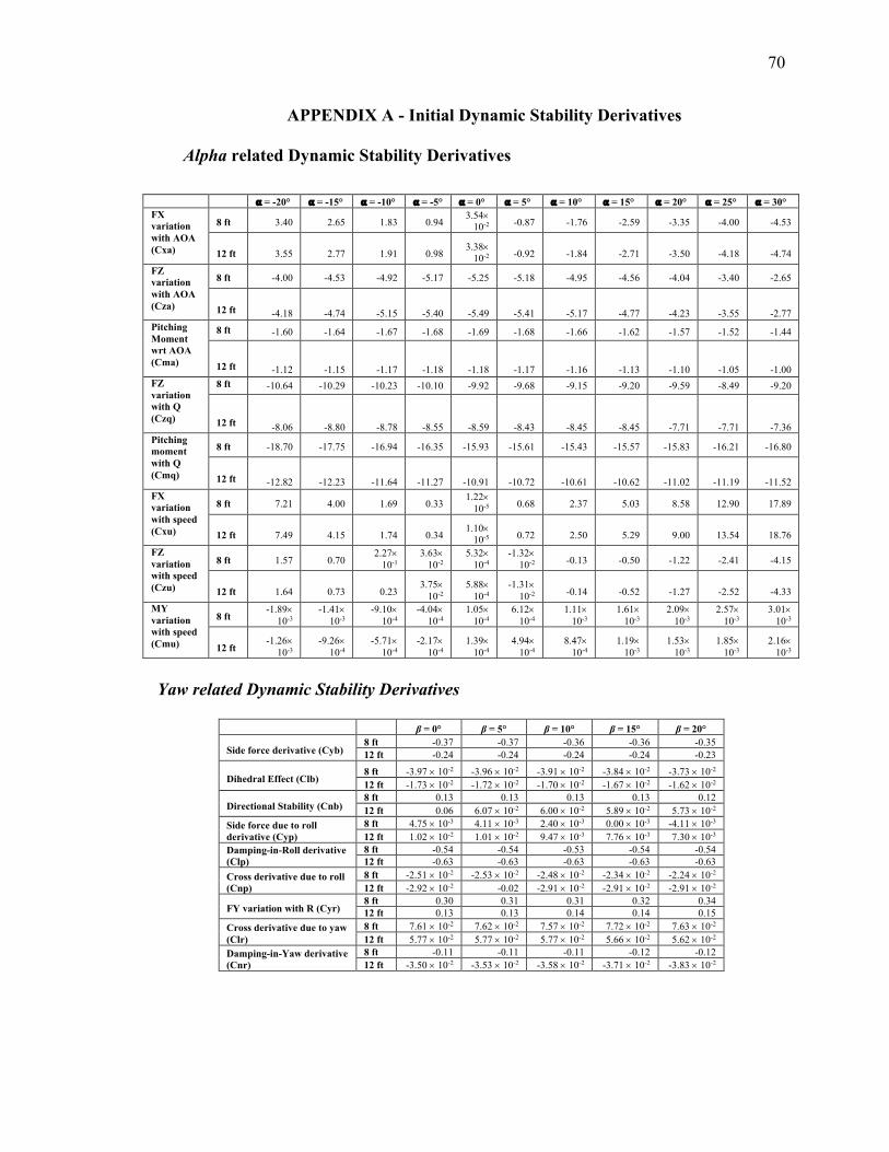
70

APPENDIX A - Initial Dynamic Stability Derivatives

Alpha related Dynamic Stability Derivatives

Yaw related Dynamic Stability Derivatives

β = 0° β = 5° β = 10° β = 15° β = 20°

Side force derivative (Cyb) 8 ft -0.37 -0.37 -0.36 -0.36 -0.35 12 ft -0.24 -0.24 -0.24 -0.24 -0.23

Dihedral Effect (Clb) 8 ft -3.97 ´ 10-2 -3.96 ´ 10-2 -3.91 ´ 10-2 -3.84 ´ 10-2 -3.73 ´ 10-2 12 ft -1.73 ´ 10-2 -1.72 ´ 10-2 -1.70 ´ 10-2 -1.67 ´ 10-2 -1.62 ´ 10-2

Directional Stability (Cnb) 8 ft 0.13 0.13 0.13 0.13 0.12 12 ft 0.06 6.07 ´ 10-2 6.00 ´ 10-2 5.89 ´ 10-2 5.73 ´ 10-2

Side force due to roll derivative (Cyp)

8 ft 4.75 ´ 10-3 4.11 ´ 10-3 2.40 ´ 10-3 0.00 ´ 10-3 -4.11 ´ 10-3 12 ft 1.02 ´ 10-2 1.01 ´ 10-2 9.47 ´ 10-3 7.76 ´ 10-3 7.30 ´ 10-3

Damping-in-Roll derivative (Clp)

8 ft -0.54 -0.54 -0.53 -0.54 -0.54 12 ft -0.63 -0.63 -0.63 -0.63 -0.63

Cross derivative due to roll (Cnp)

8 ft -2.51 ´ 10-2 -2.53 ´ 10-2 -2.48 ´ 10-2 -2.34 ´ 10-2 -2.24 ´ 10-2 12 ft -2.92 ´ 10-2 -0.02 -2.91 ´ 10-2 -2.91 ´ 10-2 -2.91 ´ 10-2

FY variation with R (Cyr) 8 ft 0.30 0.31 0.31 0.32 0.34 12 ft 0.13 0.13 0.14 0.14 0.15

Cross derivative due to yaw (Clr)

8 ft 7.61 ´ 10-2 7.62 ´ 10-2 7.57 ´ 10-2 7.72 ´ 10-2 7.63 ´ 10-2 12 ft 5.77 ´ 10-2 5.77 ´ 10-2 5.77 ´ 10-2 5.66 ´ 10-2 5.62 ´ 10-2

Damping-in-Yaw derivative (Cnr)

8 ft -0.11 -0.11 -0.11 -0.12 -0.12 12 ft -3.50 ´ 10-2 -3.53 ´ 10-2 -3.58 ´ 10-2 -3.71 ´ 10-2 -3.83 ´ 10-2

⍺ = -20° ⍺ = -15° ⍺ = -10° ⍺ = -5° ⍺ = 0° ⍺ = 5° ⍺ = 10° ⍺ = 15° ⍺ = 20° ⍺ = 25° ⍺ = 30° FX variation with AOA (Cxa)

8 ft 3.40 2.65 1.83 0.94 3.54´

10-2 -0.87 -1.76 -2.59 -3.35 -4.00 -4.53

12 ft 3.55 2.77 1.91 0.98 3.38´

10-2 -0.92 -1.84 -2.71 -3.50 -4.18 -4.74

FZ variation with AOA (Cza)

8 ft -4.00 -4.53 -4.92 -5.17 -5.25 -5.18 -4.95 -4.56 -4.04 -3.40 -2.65

12 ft -4.18 -4.74 -5.15 -5.40 -5.49 -5.41 -5.17 -4.77 -4.23 -3.55 -2.77 Pitching Moment wrt AOA (Cma)

8 ft -1.60 -1.64 -1.67 -1.68 -1.69 -1.68 -1.66 -1.62 -1.57 -1.52 -1.44

12 ft -1.12 -1.15 -1.17 -1.18 -1.18 -1.17 -1.16 -1.13 -1.10 -1.05 -1.00 FZ variation with Q (Czq)

8 ft -10.64 -10.29 -10.23 -10.10 -9.92 -9.68 -9.15 -9.20 -9.59 -8.49 -9.20

12 ft -8.06 -8.80 -8.78 -8.55 -8.59 -8.43 -8.45 -8.45 -7.71 -7.71 -7.36 Pitching moment with Q (Cmq)

8 ft -18.70 -17.75 -16.94 -16.35 -15.93 -15.61 -15.43 -15.57 -15.83 -16.21 -16.80

12 ft -12.82 -12.23 -11.64 -11.27 -10.91 -10.72 -10.61 -10.62 -11.02 -11.19 -11.52 FX variation with speed (Cxu)

8 ft 7.21 4.00 1.69 0.33 1.22´

10-5 0.68 2.37 5.03 8.58 12.90 17.89

12 ft 7.49 4.15 1.74 0.34 1.10´

10-5 0.72 2.50 5.29 9.00 13.54 18.76

FZ variation with speed (Czu)

8 ft 1.57 0.70 2.27´

10-1 3.63´

10-2 5.32´

10-4 -1.32´

10-2 -0.13 -0.50 -1.22 -2.41 -4.15

12 ft 1.64 0.73 0.23 3.75´

10-2 5.88´

10-4 -1.31´

10-2 -0.14 -0.52 -1.27 -2.52 -4.33

MY variation with speed (Cmu)

8 ft -1.89´

10-3 -1.41´

10-3 -9.10´

10-4 -4.04´

10-4 1.05´

10-4 6.12´

10-4 1.11´

10-3 1.61´

10-3 2.09´

10-3 2.57´

10-3 3.01´

10-3

12 ft -1.26´

10-3 -9.26´

10-4 -5.71´

10-4 -2.17´

10-4 1.39´

10-4 4.94´

10-4 8.47´

10-4 1.19´

10-3 1.53´

10-3 1.85´

10-3 2.16´

10-3

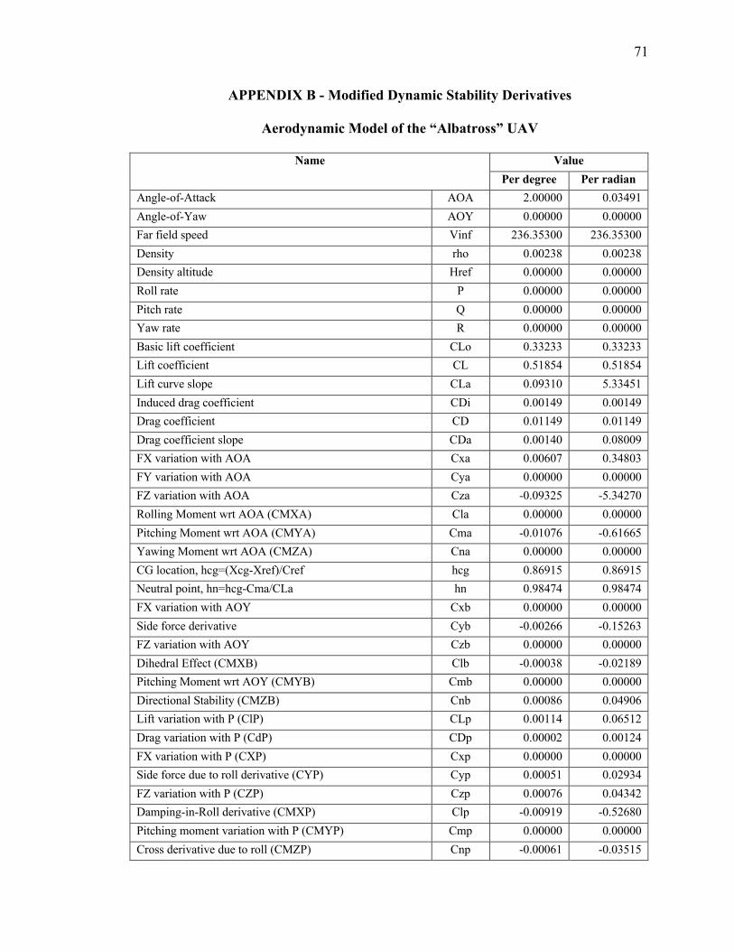
71

APPENDIX B - Modified Dynamic Stability Derivatives

Aerodynamic Model of the “Albatross” UAV

Name Value Per degree Per radian

Angle-of-Attack AOA 2.00000 0.03491 Angle-of-Yaw AOY 0.00000 0.00000 Far field speed Vinf 236.35300 236.35300 Density rho 0.00238 0.00238 Density altitude Href 0.00000 0.00000 Roll rate P 0.00000 0.00000 Pitch rate Q 0.00000 0.00000 Yaw rate R 0.00000 0.00000 Basic lift coefficient CLo 0.33233 0.33233 Lift coefficient CL 0.51854 0.51854 Lift curve slope CLa 0.09310 5.33451 Induced drag coefficient CDi 0.00149 0.00149 Drag coefficient CD 0.01149 0.01149 Drag coefficient slope CDa 0.00140 0.08009 FX variation with AOA Cxa 0.00607 0.34803 FY variation with AOA Cya 0.00000 0.00000 FZ variation with AOA Cza -0.09325 -5.34270 Rolling Moment wrt AOA (CMXA) Cla 0.00000 0.00000 Pitching Moment wrt AOA (CMYA) Cma -0.01076 -0.61665 Yawing Moment wrt AOA (CMZA) Cna 0.00000 0.00000 CG location, hcg=(Xcg-Xref)/Cref hcg 0.86915 0.86915 Neutral point, hn=hcg-Cma/CLa hn 0.98474 0.98474 FX variation with AOY Cxb 0.00000 0.00000 Side force derivative Cyb -0.00266 -0.15263 FZ variation with AOY Czb 0.00000 0.00000 Dihedral Effect (CMXB) Clb -0.00038 -0.02189 Pitching Moment wrt AOY (CMYB) Cmb 0.00000 0.00000 Directional Stability (CMZB) Cnb 0.00086 0.04906 Lift variation with P (ClP) CLp 0.00114 0.06512 Drag variation with P (CdP) CDp 0.00002 0.00124 FX variation with P (CXP) Cxp 0.00000 0.00000 Side force due to roll derivative (CYP) Cyp 0.00051 0.02934 FZ variation with P (CZP) Czp 0.00076 0.04342 Damping-in-Roll derivative (CMXP) Clp -0.00919 -0.52680 Pitching moment variation with P (CMYP) Cmp 0.00000 0.00000 Cross derivative due to roll (CMZP) Cnp -0.00061 -0.03515

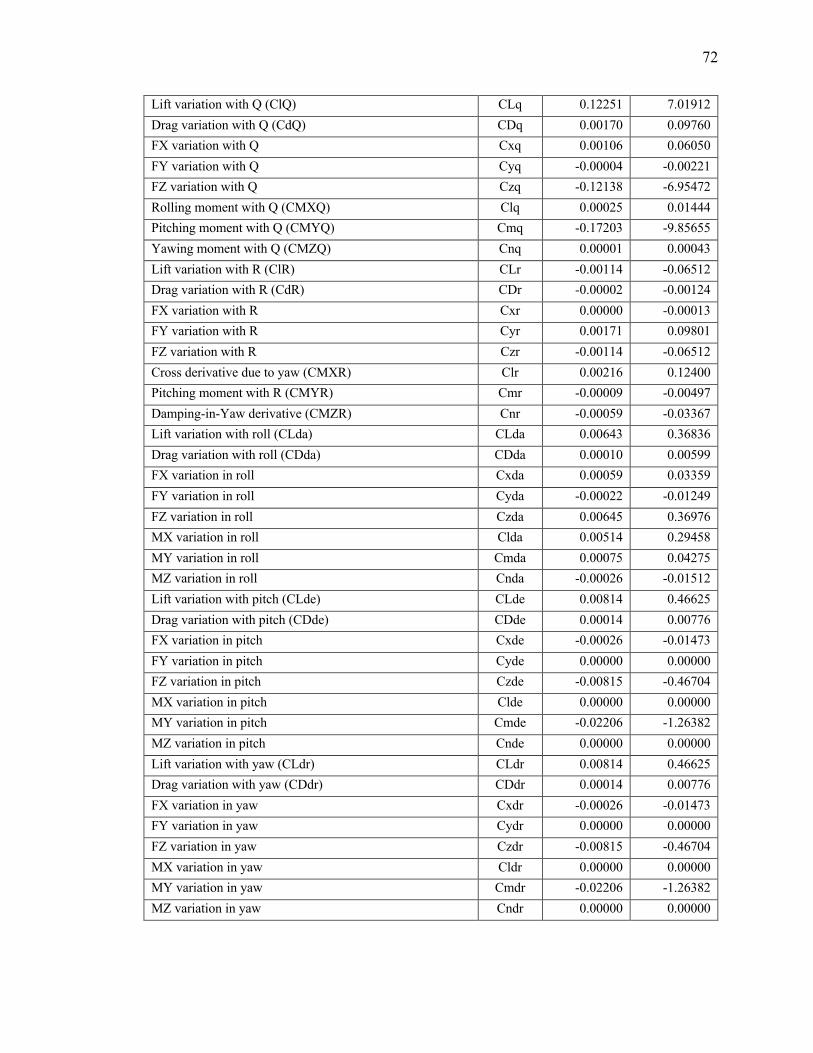
72

Lift variation with Q (ClQ) CLq 0.12251 7.01912 Drag variation with Q (CdQ) CDq 0.00170 0.09760 FX variation with Q Cxq 0.00106 0.06050 FY variation with Q Cyq -0.00004 -0.00221 FZ variation with Q Czq -0.12138 -6.95472 Rolling moment with Q (CMXQ) Clq 0.00025 0.01444 Pitching moment with Q (CMYQ) Cmq -0.17203 -9.85655 Yawing moment with Q (CMZQ) Cnq 0.00001 0.00043 Lift variation with R (ClR) CLr -0.00114 -0.06512 Drag variation with R (CdR) CDr -0.00002 -0.00124 FX variation with R Cxr 0.00000 -0.00013 FY variation with R Cyr 0.00171 0.09801 FZ variation with R Czr -0.00114 -0.06512 Cross derivative due to yaw (CMXR) Clr 0.00216 0.12400 Pitching moment with R (CMYR) Cmr -0.00009 -0.00497 Damping-in-Yaw derivative (CMZR) Cnr -0.00059 -0.03367 Lift variation with roll (CLda) CLda 0.00643 0.36836 Drag variation with roll (CDda) CDda 0.00010 0.00599 FX variation in roll Cxda 0.00059 0.03359 FY variation in roll Cyda -0.00022 -0.01249 FZ variation in roll Czda 0.00645 0.36976 MX variation in roll Clda 0.00514 0.29458 MY variation in roll Cmda 0.00075 0.04275 MZ variation in roll Cnda -0.00026 -0.01512 Lift variation with pitch (CLde) CLde 0.00814 0.46625 Drag variation with pitch (CDde) CDde 0.00014 0.00776 FX variation in pitch Cxde -0.00026 -0.01473 FY variation in pitch Cyde 0.00000 0.00000 FZ variation in pitch Czde -0.00815 -0.46704 MX variation in pitch Clde 0.00000 0.00000 MY variation in pitch Cmde -0.02206 -1.26382 MZ variation in pitch Cnde 0.00000 0.00000 Lift variation with yaw (CLdr) CLdr 0.00814 0.46625 Drag variation with yaw (CDdr) CDdr 0.00014 0.00776 FX variation in yaw Cxdr -0.00026 -0.01473 FY variation in yaw Cydr 0.00000 0.00000 FZ variation in yaw Czdr -0.00815 -0.46704 MX variation in yaw Cldr 0.00000 0.00000 MY variation in yaw Cmdr -0.02206 -1.26382 MZ variation in yaw Cndr 0.00000 0.00000

Documents

Design and Flight-Path Simulation of a Dynamic-Soaring UAV