Embed Size (px)
Citation preview

Design and Evaluation of a Single-Span Bridge Using Ultra-High Performance Concrete
Final ReportSeptember 2009
Sponsored byFederal Highway AdministrationIowa Highway Research Board (TR-529)Wapello County, Iowa

About the BEC
The mission of the Bridge Engineering Center is to conduct research on bridge technologies to help bridge designers/owners design, build, and maintain long-lasting bridges.
Disclaimer Notice
The contents of this report reflect the views of the authors, who are responsible for the facts and the accuracy of the information presented herein. The opinions, findings and conclusions expressed in this publication are those of the authors and not necessarily those of the sponsors.
The sponsors assume no liability for the contents or use of the information contained in this document. This report does not constitute a standard, specification, or regulation.
The sponsors do not endorse products or manufacturers. Trademarks or manufacturers’ names appear in this report only because they are considered essential to the objective of the document.
Non-discrimination Statement
Iowa State University does not discriminate on the basis of race, color, age, religion, national origin, sexual orientation, gender identity, sex, marital status, disability, or status as a U.S. veteran. Inquiries can be directed to the Director of Equal Opportunity and Diversity, (515) 294-7612.
Iowa Department of Transportation Statements
Federal and state laws prohibit employment and/or public accommodation discrimination on the basis of age, color, creed, disability, gender identity, national origin, pregnancy, race, religion, sex, sexual orientation or veteran’s status. If you believe you have been discriminated against, please contact the Iowa Civil Rights Commission at 800-457-4416 or Iowa Department of Transportation’s affirmative action officer. If you need accommodations because of a disability to access the Iowa Department of Transportation’s services, contact the agency’s affirmative action officer at 800-262-0003.
The preparation of this (report, document, etc.) was financed in part through funds provided by the Iowa Department of Transportation through its “Agreement for the Management of Research Conducted by Iowa State University for the Iowa Department of Transportation,” and its amendments.
The opinions, findings, and conclusions expressed in this publication are those of the authors and not necessarily those of the Iowa Department of Transportation.

Technical Report Documentation Page
1. Report No. 2. Government Accession No. 3. Recipient’s Catalog No.
4. Title and Subtitle 5. Report Date
Design and Evaluation of a Single-span Bridge Using Ultra-High Performance Concrete
September 2009
6. Performing Organization Code
7. Author(s) 8. Performing Organization Report No.
9. Performing Organization Name and Address 10. Work Unit No. (TRAIS)
Center for Transportation Research and Education
Iowa State University
2711 South Loop Drive, Suite 4700
Ames, IA 50010-8664
11. Contract or Grant No.
12. Sponsoring Organization Name and Address 13. Type of Report and Period Covered
Iowa Department of Transportation
800 Lincoln Way
Ames, IA 50010
14. Sponsoring Agency Code
15. Supplementary Notes
Funding provided through the Innovative Bridge Research and Construction Program within the Federal Highway Administration and the Iowa Highway Research Board. Wapello County received the FHWA funds directly and contracted with Iowa State University.
16. Abstract
Research presented herein describes an application of a newly developed material called Ultra-High Performance Concrete (UHPC) to a single-span bridge. The two primary objectives of this research were to develop a shear design procedure for possible code adoption and to provide a performance evaluation to ensure the viability of the first UHPC bridge in the United States. Two other secondary objectives included defining of material properties and understanding of flexural behavior of a UHPC bridge girder. In order to obtain information in these areas, several tests were carried out including material testing, large-scale laboratory flexure testing, large-scale laboratory shear testing, large-scale laboratory flexure-shear testing, small-scale laboratory shear testing, and field testing of a UHPC bridge.
Experimental and analytical results of the described tests are presented. Analytical models to understand the flexure and shear behavior of UHPC members were developed using iterative computer based procedures. Previous research is referenced explaining a simplified flexural design procedure and a simplified pure shear design procedure. This work describes a shear design procedure based on the Modified Compression Field Theory (MCFT) which can be used in the design of UHPC members. Conclusions are provided regarding the viability of the UHPC bridge and recommendations are made for future research.
17. Key Words 18. Distribution Statement
Ultra High Performance Concrete, UHPC, Testing, Bridge Testing, Material Testing
No restrictions.
19. Security Classification (of this report)
20. Security Classification (of this page)
21. No. of Pages 22. Price
Unclassified. Unclassified. 148 NA
IHRB Project TR-529
Terry J. Wipf, Brent M. Phares, Sri Sritharan, Brian E. Degen, Mark T. Giesmann
Final Report


DESIGN AND EVALUATION OF A SINGLE-SPAN
BRIDGE USING ULTRA-HIGH PERFORMANCE
CONCRETE
Co-Principal Investigators Terry J. Wipf, P.E.
Professor of Civil Engineering, Iowa State University Director of the Bridge Engineering Center
Center for Transportation Research and Education
Brent M. Phares, P.E. Associate Director of the Bridge Engineering Center Center for Transportation Research and Education
Sr Sritharan
Associate Professor of Civil Engineering, Iowa State University
Research Assistant Brian E. Degen
Mark T. Giesmann
Authors Terry J. Wipf, Brent M. Phares, Sri Sritharan, Brian E. Degen, Mark T. Giesmann
Preparation of this report was financed in part
through funds provided by the Iowa Department of Transportation through its research management agreement with the Center for Transportation Research and Education.
Institute for Transportation
Iowa State University 2711 South Loop Drive, Suite 4700
Ames, IA 50010-8664 Phone: 515-294-8103 Fax: 515-294-0467
www.intrans.iastate.edu
Final Report September 2009


v
TABLE OF CONTENTS
ACKNOWLEDGMENTS ............................................................................................................. xi
CHAPTER 1: INTRODUCTION ...................................................................................................1
1.1 Background ...................................................................................................................1 1.2 Concrete Types .............................................................................................................1 1.3 Advantages and Disadvantages of UHPC.....................................................................3 1.4 Research Objectives ......................................................................................................4 1.5 Project Scope ................................................................................................................4 1.6 Conventions ..................................................................................................................4 1.7 Report Content ..............................................................................................................5
CHAPTER 2: LITERATURE REVIEW ........................................................................................7
2.1 Material Properties ........................................................................................................7 2.2 Flexural Strength .........................................................................................................11 2.3 Shear Strength .............................................................................................................12 2.4 Structural Testing ........................................................................................................23 2.5 Prestress Bond .............................................................................................................24
CHAPTER 3: FIELD BRIDGE DESCIPTION ............................................................................27
3.1 Design .........................................................................................................................28 3.2 Construction ................................................................................................................29
CHAPTER 4: EXPERIMENTAL TEST PROGRAM .................................................................33
4.1 Material Testing ..........................................................................................................33 4.1.1 Uniaxial Compression Testing .....................................................................33
4.1.1.1 Test Specimen Description ...........................................................33 4.1.1.2 Test Configuration ........................................................................33 4.1.1.3 Test Procedure ..............................................................................33
4.1.2 Prism Flexural Testing .................................................................................34 4.1.2.1 Test Specimen Description ...........................................................34 4.1.2.2 Test Configuration ........................................................................34 4.1.2.3 Test Procedure ..............................................................................35
4.2 Large-Scale Laboratory Testing .................................................................................35 4.2.1 Test Specimen Description ..........................................................................35
4.2.1.1 Design ...........................................................................................36 4.2.1.2 Construction ..................................................................................36
4.2.2 Flexural Testing ..........................................................................................36 4.2.2.1 Test Configuration ........................................................................36 4.2.2.2 Test Procedure ..............................................................................38
4.2.3 Shear Testing ...............................................................................................39 4.2.3.1 Test Configuration ........................................................................39 4.2.3.2 Test Procedure ..............................................................................39

vi
4.2.4 Flexure-Shear Testing ..................................................................................41 4.2.4.1 Test Configuration ........................................................................41 4.2.4.2 Test Procedure ..............................................................................44
4.3 Small-Scale Laboratory Testing .................................................................................44 4.3.1 Test Specimen Description ..........................................................................44
4.3.1.1 Design ...........................................................................................46 4.3.1.2 Construction ..................................................................................46 4.3.1.3 Test Configuration ........................................................................46
4.3.2 Test Procedure .............................................................................................48 4.4 Field Testing ...............................................................................................................49
4.4.1 Release Testing ............................................................................................50 4.4.1.1 Test Configuration ........................................................................50 4.4.1.2 Test Procedure ..............................................................................50
4.4.2 Dead Load Testing .......................................................................................50 4.4.2.1 Test Configuration ........................................................................50 4.4.2.2 Test Procedure ..............................................................................51
4.4.3 Live Load Testing ........................................................................................51 4.4.3.1 Test Configuration ........................................................................51 4.4.3.2 Test Procedure ..............................................................................52 4.4.3.3 Pseudo-Static Loading ..................................................................52 4.4.3.4 Dynamic Loading ..........................................................................52
CHAPTER 5: ANALYSIS METHODS .......................................................................................57
5.1 Uncracked Beam Analysis ..........................................................................................57 5.1.1 Sectional Analysis ........................................................................................57 5.1.2 Deflection Analysis ......................................................................................59
5.2 Cracked Beam Analysis ..............................................................................................60 5.2.1 Sectional Analysis ........................................................................................60
5.2.1.1 Flexural Analysis ..........................................................................60 5.2.1.2 Flexure and Shear Analysis ..........................................................65
5.2.2 Deflection Analysis ......................................................................................74 5.2.3 Strut and Tie Analysis ..................................................................................75
CHAPTER 6: EXPERIMENTAL AND ANALYTICAL RESULTS ..........................................77
6.1 Material Testing ..........................................................................................................77 6.1.1 Uniaxial Compression Testing .....................................................................77 6.1.2 Prism Flexural Testing .................................................................................77
6.2 Large-Scale Laboratory Testing .................................................................................78 6.2.1 Flexural Testing ...........................................................................................78
6.2.1.1 Test Observations .........................................................................78 6.2.1.2 Test Results ...................................................................................79
6.2.2 Shear Testing ...............................................................................................82 6.2.2.1 Test Observations .........................................................................82 6.2.2.2 Test Results ...................................................................................83
6.2.3 Flexure-Shear Testing ..................................................................................88 6.2.3.1 Test Observations .........................................................................88

vii
6.2.3.2 Test Results ...................................................................................89 6.3 Small-Scale Laboratory Testing .................................................................................93
6.3.1 Test Observations ........................................................................................93 6.3.2 Test Results ..................................................................................................97
6.4 Field Testing .............................................................................................................101 6.4.1 Release Testing ..........................................................................................101 6.4.2 Dead Load Testing .....................................................................................103 6.4.3 Live Load Testing ......................................................................................104
6.4.3.1 Test 1 Results ..............................................................................105 6.4.3.2 Test 2 Results ..............................................................................111 6.4.3.3 Comparative Results ...................................................................116
CHAPTER 7: RECOMMENDED SHEAR DESIGN PROCEDURE .......................................119
7.1 Service Limit State ....................................................................................................119 7.1.1 Procedure Description ................................................................................119 7.1.2 Conservatism of Procedure ........................................................................120
7.2 Ultimate Limit State ..................................................................................................121 7.2.1 Procedure Description ................................................................................121 7.2.2 Conservatism of Procedure ........................................................................125
CHAPTER 8: CONCLUSIONS .................................................................................................129
8.1 Performance Evaluation ............................................................................................130 8.2 Future Research of UHPC ........................................................................................131
REFERENCES ............................................................................................................................132


ix
LIST OF FIGURES Figure 1.1. Wapello County truss bridge prior to replacement. .....................................................1 Figure 1.2. Samples of UHPC and conventional concrete. ............................................................3 Figure 2.1. Compressive constitutive properties of UHPC. ...........................................................7 Figure 2.2. Tensile constitutive properties of UHPC. .....................................................................8 Figure 2.3. Tensile constitutive properties of UHPC tested by Chuang and Ulm [2]. .................10 Figure 2.4. General strut and tie truss model. ...............................................................................13 Figure 2.5. Average and local stresses transmitted across cracks used by the MCFT [5]. ...........17 Figure 2.6. Mohr’s circle of average concrete stresses in a general concrete element [5]. ..........18 Figure 2.7. Vertical forces used in MCFT equilibrium condition. ...............................................19 Figure 2.8. Mohr’s circle of average concrete strains in a general concrete element [5]. ............20 Figure 2.9. FHWA flexure and shear testing setup diagrams. ......................................................24 Figure 2.10. FHWA flexure test setup photograph. ......................................................................24 Figure 2.11. Prismatic cross section of AASHTO type II FHWA test beam. ..............................25 Figure 2.12. Pull-out test apparatus used by Lubbers [13]. ..........................................................25 Figure 2.13. Pull-out test data for 0.5 in. oversized strands [13]. .................................................26 Figure 3.1. Cross section of Wapello County UHPC bridge. .......................................................27 Figure 3.2. Cross sections of Wapello County UHPC bridge beams. ..........................................28 Figure 3.3. Elevation of Wapello County UHPC bridge beams. ..................................................28 Figure 3.4. Placement of concrete during construction of Wapello County UHPC bridge
beams. ................................................................................................................................30 Figure 3.5. Elevation of Wapello County UHPC bridge. .............................................................31 Figure 4.1. Uniaxial compression test setup used for UHPC cubes. ............................................34 Figure 4.2. Flexure test setup used for UHPC prisms. .................................................................35 Figure 4.3. Large-scale flexure test setup diagram. ......................................................................37 Figure 4.4. Large-scale flexure test setup photograph. .................................................................37 Figure 4.5. Instrumentation on east side for large-scale flexure test. ...........................................37 Figure 4.6. Instrumentation on west side for large-scale flexure test. ..........................................38 Figure 4.7. Large-scale shear test setup diagram. .........................................................................39 Figure 4.8. Large-scale shear test setup photograph. ....................................................................40 Figure 4.9. Instrumentation on east side for large-scale shear test. ..............................................40 Figure 4.10. Instrumentation on west side for large-scale shear test. ...........................................40 Figure 4.11. Large strain rosettes gages R1 and R2 used for large-scale shear test. ....................41 Figure 4.12. Large-scale flexure-shear test setup diagram. ..........................................................41 Figure 4.13. Large-scale flexure-shear test setup photograph. .....................................................42 Figure 4.14. Instrumentation on east side for large-scale flexure-shear test. ...............................42 Figure 4.15. Instrumentation on west side for large-scale flexure-shear test. ..............................43 Figure 4.16. Large strain rosette gage R1 used for large-scale flexure-shear test. .......................43 Figure 4.17. Cross sections of small-scale test beams. .................................................................45 Figure 4.17. Cross sections of small-scale test beams (continued). .............................................46 Figure 4.18. Typical small-scale test setup. ..................................................................................47 Figure 4.19. 10-in. beam test setup. ..............................................................................................47 Figure 4.20. Instrumentation of 10-in. beams. ..............................................................................48 Figure 4.21. 12-in. beam test setup. ..............................................................................................49 Figure 4.22. Instrumentation of 12-in. beams. ..............................................................................49 Figure 4.23. Fiber optic gage locations in the large-scale test beam. ...........................................50

x
Figure 4.24. Fiber optic gage locations in the bridge beam. .........................................................50 Figure 4.25. BDI strain transducers attached to concrete. ............................................................51 Figure 4.26. Location of BDI strain transducers used during both tests. .....................................53 Figure 4.27. Test vehicle used in Test 1. ......................................................................................54 Figure 4.28. Test vehicle used in Test 2. ......................................................................................55 Figure 4.29. Truck positions used in the live load tests. ...............................................................56 Figure 5.1. General strain, stress, and shear within a section. ......................................................60 Figure 5.2. UHPC compressive and tensile constitutive properties. ............................................61 Figure 5.3. Prestressing strand tensile constitutive properties. .....................................................62 Figure 5.4. UHPC strain profile at midspan of large-scale flexure test beam at nominal moment
strength. ..............................................................................................................................62 Figure 5.5. UHPC stress profile at midspan of large-scale flexure test beam at nominal moment
strength. ..............................................................................................................................63 Figure 5.6. Strand strain profile at midspan of large-scale flexure test beam at nominal moment
strength. ..............................................................................................................................63 Figure 5.7. Strand stress profile at midspan of large-scale flexure test beam at nominal moment
strength. ..............................................................................................................................64 Figure 5.8. Force resultants at midspan of large-scale flexure test beam at nominal moment
strength. ..............................................................................................................................64 Figure 5.9. Directions of stresses and strains in a general UHPC element...................................65 Figure 5.10. Mohr’s circle of average concrete stresses in a general UHPC element [5]. ...........69 Figure 5.11. Mohr’s circle of average concrete strains in a general UHPC element [5]. .............69 Figure 5.12. Unsoftened longitudinal stress of large-scale flexure-shear test beam at load
application point L4 while undergoing a total load of 600 kips. .......................................72 Figure 5.13. Vertical strain of large-scale flexure-shear test beam at load application point L4
while undergoing a total load of 600 kips. .........................................................................72 Figure 5.14. Principal compressive stress angle of large-scale flexure-shear test beam at load
application point L4 while undergoing a total load of 600 kips. .......................................73 Figure 5.15. Softening coefficient of large-scale flexure-shear test beam at load application
point L4 while undergoing a total load of 600 kips. ..........................................................73 Figure 5.16. Softened longitudinal stress of large-scale flexure-shear test beam at load
application point L4 while undergoing a total load of 600 kips. .......................................74 Figure 5.17. Deflection of FHWA Flexure Test beam at midspan. ..............................................75 Figure 5.18. Deflection of FHWA Shear Test #2 beam at the load application point. .................76 Figure 6.1. Load vs. table displacement during a typical prism flexure test. ...............................78 Figure 6.2. Flexural cracks on north bottom flange at midspan at peak load of large-scale flexure
test. .....................................................................................................................................79 Figure 6.3. Strain at midspan during large-scale flexure test. ......................................................80 Figure 6.4. Deflection at midspan during large-scale flexure test. ...............................................81 Figure 6.5. Longitudinal live load stresses at cracking of large-scale flexure test beam. ............81 Figure 6.6. Strand slip at gage S1 during large-scale flexure test. ...............................................82 Figure 6.7. Shear crack at west end of large-scale shear test beam after failure. .........................83 Figure 6.8. Vertical crack in web at west end of large-scale shear test beam after failure. .........83 Figure 6.9. Strain at gage #2 during large-scale shear test. ..........................................................84 Figure 6.10. Strain at gage #10 during large-scale shear test. ......................................................85 Figure 6.11. Deflection including shear analysis at gage D3 during large-scale shear test. ........85 Figure 6.12. Deflection excluding shear analysis at gage D3 during large-scale shear test. ........86 Figure 6.13. Strand slip at gage S3 during large-scale shear test. ................................................87

xi
Figure 6.14. Live load principal stresses at gage #2 during large-scale shear test. ......................87 Figure 6.15. Total load principal stresses at gage #2 during large-scale shear test. .....................88 Figure 6.16. Flexure and shear cracking near gage R1 at a total load of 482 kips during the
large-scale flexure-shear test. ............................................................................................89 Figure 6.17. Strain at gage F5 during large-scale flexure-shear test. ...........................................90 Figure 6.18. Strain at gage #17 during large-scale flexure-shear test. .........................................90 Figure 6.19. Deflection at gage D5 during large-scale flexure-shear test. ...................................91 Figure 6.20. Live load principal stresses at gage #17 during large-scale flexure-shear test. .......91 Figure 6.21. Total load principal stresses at gage #17 during large-scale flexure-shear test. ......92 Figure 6.22. Shear constitutive properties of UHPC. ...................................................................92 Figure 6.23. Cracking of small-scale test beams after failure. .....................................................95 Figure 6.23. Cracking of small-scale test beams after failure (continued). ..................................96 Figure 6.23. Cracking of small-scale test beams after failure (continued). ..................................97 Figure 6.24. Deflection at gage D1 of small-scale test beam C2. .................................................99 Figure 6.25. Total load principal stresses at gage #7 of small-scale test beam C2. .....................99 Figure 6.26. Deflection at gage D3 of small-scale test beam E1. ...............................................100 Figure 6.27. Deflection at gage D2 of small-scale test beam E1. ...............................................100 Figure 6.28. Strand slip at gage S1 of small-scale test beam E1. ...............................................101 Figure 6.29. Strand slip at gage S3 of small-scale test beam E1. ...............................................101 Figure 6.30. Strains at gage F3 of large-scale test beam during strand release. .........................102 Figure 6.31. Strains at gage F3 of bridge beam during deck pour. .............................................103 Figure 6.32. Stresses at gage F3 of bridge beam during deck pour. ...........................................104 Figure 6.33. Stresses at gage F4 of bridge beam during deck pour. ...........................................105 Figure 6.34. Maximum bottom flange girder strains at midspan for Test 1. ..............................106 Figure 6.35. Neutral axis location of girders at midspan for Test 1. ..........................................107 Figure 6.35. Neutral axis location of girders at midspan for Test 1 (continued). .......................108 Figure 6.36. Experimental load fractions from Test 1. ...............................................................109 Figure 6.37. Experimental and AASHTO distribution factors from Test 1. ..............................110 Figure 6.38. Bottom flange midspan girder strain versus time, Load Case 7, Test 1. ................111 Figure 6.39. Maximum bottom flange girder strains at midspan for Test 2. ..............................112 Figure 6.40. Neutral axis location of girders at midspan for Test 2. ..........................................113 Figure 6.40. Neutral axis location of girders at midspan for Test 2 (continued). .......................114 Figure 6.41. Experimental load fractions from Test 2. ...............................................................115 Figure 6.42. Experimental and AASHTO distribution factors from Test 2. ..............................115 Figure 6.43. Bottom flange midspan girder strain versus time, Load Case 7, Test 2. ................116 Figure 6.44. Bottom flange girder strains at midspan from Test 1 and Test 2. ..........................117 Figure 6.45. Distribution factors from Test 1 and Test 2. ..........................................................118 Figure 7.1. Bridge loading required by AASHTO. .....................................................................120 Figure 7.2. Tensile stresses within a general beam at the ultimate loading condition according to
the MCFT. ........................................................................................................................122 Figure 7.3. Applied forces within the longitudinal reinforcement of a general beam at the
ultimate loading condition according to the MCFT. ........................................................123 Figure 7.4. Recommended and MCFT Sections at which to perform analysis. .........................125

xii
LIST OF TABLES Table 1.1. Typical UHPC material composition [1]. ......................................................................2 Table 1.2. Advantages and disadvantages of UHPC. .....................................................................4 Table 1.3. Sign conventions. ...........................................................................................................5 Table 2.1. Compressive and tensile constitutive properties of UHPC. ...........................................8 Table 2.2. Compressive strength of 3x6 in. UHPC cylinders tested by Graybeal and Hartmann
[1]. ........................................................................................................................................9 Table 2.3. Tensile cracking strength of UHPC tested by Graybeal and Hartmann [1]. .................9 Table 2.4. MCFT shear design factors for concrete members with web reinforcement [11]. ......23 Table 4.1. Location of strain gages used in large-scale flexure test. ............................................38 Table 4.2. Location of strain gages used in large-scale flexure-shear test. ..................................43 Table 4.3. Initial prestress and length of small-scale test beams. .................................................46 Table 4.4. Variables in the setup of the 10-in. small-scale test beams. ........................................47 Table 4.5. Summary of test vehicle’s axle loads for Test 1. .........................................................54 Table 4.6. Summary of test vehicle’s axle loads for Test 2. .........................................................55 Table 6.1. Uniaxial compressive strength of UHPC cubes. ..........................................................77 Table 6.2. Flexural cracking tensile strength of UHPC prisms. ...................................................78 Table 6.3. Comparison of large-scale flexure test capacities to applied bridge moments. ...........80 Table 6.4. Live load applied at three events during the large-scale shear test. ............................83 Table 6.5. Comparison of large-scale shear test capacities to applied bridge shears. ..................84 Table 6.6. Live load applied at three events during the large-scale flexure-shear test. ................89 Table 6.7. Live load and shear force applied at cracking and failure of the small-scale test
beams. ................................................................................................................................93 Table 6.8. Failure modes of small-scale test beams. ....................................................................94 Table 6.9. Comparison of experimental and analytical live loads required to cause cracking and
failure of the small-scale test beams. .................................................................................98 Table 6.10. Stresses in large-scale test beam after strand release. .............................................102 Table 6.11. Stresses in bridge beam after strand release. ...........................................................103 Table 7.1. Analytical cracking stress calculated at experimental cracking load for all beam
tests. .................................................................................................................................120 Table 7.2. Experimental and analytical ultimate shear strength of small-scale test beams. .......126 Table 7.3. Comparison of calculated and allowable longitudinal strains at failure of the large-
scale shear and flexure-shear tests. ..................................................................................127

xiii
ACKNOWLEDGMENTS
The authors would like to thank the Iowa Department of Transportation, Wapello County, and the Federal Highway Administration for providing funding, design expertise, and research collaboration. In particular Dean Bierwagen from the Iowa Department of Transportation and Brain Moore from Wapello County have had instrumental involvement with this project. Lafarge North America has shared expertise on the construction, research, and design of Ultra-High Performance Concrete. The Federal Highway Administration has provided research collaboration and test equipment. Special thanks are accorded to Doug Wood, Structures Laboratory Manager at Iowa State University, for his assistance in various phases of experimental testing.


1
CHAPTER 1: INTRODUCTION
1.1 Background
In 2003 the Iowa Department of Transportation (Iowa DOT) and Wapello County, Iowa began planning for a bridge replacement project. At that time, the bridge (see Fig. 1.1) known as FHWA structure #330530 100th Ave. over Little Soap Creek was closed due to durability and strength concerns. This bridge was a steel truss bridge with a timber deck and timber abutments. The need and timing for a bridge replacement presented an opportunity to use a newly developed material called Ultra-High Performance Concrete (UHPC). Ultimately, this became the first UHPC bridge constructed in the United States and construction was partially funded through the Federal Highway Administration’s (FHWA) Innovative Bridge Research and Construction (IBRC) program.
Figure 1.1. Wapello County truss bridge prior to replacement.
1.2 Concrete Types
One general way of classifying concrete is within the following three categories: conventional concrete, High Performance Concrete (HPC), and UHPC. Conventional concrete generally has compressive strengths of at least 2,000 psi with maximum design strengths of approximately 6,000 psi. In general, the material components in conventional concrete include coarse aggregate, fine aggregate, cement, and water. Fundamentally, the cement and water undergo a chemical reaction thereby creating a hardened paste that binds the aggregate together.

2
Generally, HPC has compressive strengths in the range of approximately 6,000 psi to 16,000 psi. In addition to the material components of conventional concrete, HPC can contain silica fume, fly ash, retarder, and superplasticizer. Silica fume and fly ash act as extremely fine aggregate, filling voids in the concrete mix and thereby creating a denser and stronger material. Generally in all concretes, the less water compared with the amount of cement that exists, the stronger the concrete. Accelerator is a chemical that allows the water to cement ratio to be reduced by delaying the concrete from setting up to allow time to place the material. Superplasticizer is a chemical that allows the water to cement ratio to be further reduced by liquefying the concrete, thus allowing placement of the material with improved workability.
The compressive strength of UHPC is generally 16,000 psi to 30,000 psi. Also, the tensile strength ofUHPC, which is normally negligible and therefore neglected in other concretes, can be as high as 1,700 psi. Refer to section 2.1 on the material properties of UHPC. The material components of UHPC can include all of the materials previously listed except for coarse aggregate. The exclusion of coarse aggregate filler material, which is generally weaker than other components, makes a stronger concrete possible. UHPC also contains small fibers, either steel or organic, randomly mixed within the concrete. The steel fibers used for this research constitute 2% of the mix by volume and they are 0.006 in. in diameter and 05 in. in length. These fibers increase both the material’s tensile strength and its ductility. Refer to Table 1.1 for a typical material composition of UHPC. For comparison, Fig. 1.2 shows samples of UHPC and conventional concrete. The darker colored square samples are composed of UHPC and the presence of steel fibers is apparent. The conventional concrete, in the light circular samples shows the presence of coarse aggregate which is not a component in UHPC.
UHPC materials may be referred to by several names. The term Reactive Powder Concrete is sometimes used in the academic world to describe UHPC. UHPC may also be identified as Fiber Reinforced Concrete referring to the use of the fibers. All the research summarized herein referring to UHPC has been conducted on one specific brand name of UHPC manufactured by Lafarge North America and known as Ductal®.
Table 1.1. Typical UHPC material composition [1].
Material Amount (lb/cubic yard)Portland Cement 1200
Fine Sand 1720Silica Fume 390
Ground Quartz 355Superplasticizer 51.8
Accelerator 50.5Steel Fibers 263
Water 184
3
Figure 1.2. Samples of UHPC and conventional concrete.
1.3 Advantages and Disadvantages of UHPC
Several characteristics of UHPC make it a desirable construction material. With increased compressive and tensile strengths, the material lends itself well to structural applications by allowing greater loads to be supported. By utilizing the higher strengths, traditional structural components can also be reduced in size and weight. Another benefit of UHPC is the high density of the material making it essentially impermeable to water and chlorides, thus making the material highly durable. Both characteristics also make UHPC attractive in areas of high impact and where water or chloride ions can corrode steel reinforcement.
Although not discussed in detail here, the life-cycle cost of UHPC may prove to be lower than other concretes. UHPC material itself is more costly than conventional and high performance concretes due to the elimination of the less expensive coarse aggregate material, the use of more cement, and the addition of fibers. However, the labor cost associated with creating a structural component such as a beam can be reduced. This is because the steel fibers are mixed within the concrete matrix in a random orientation as compared to other concretes where larger steel reinforcing bars must be hand placed in specific orientations. Additionally, in some cases steel reinforcement may potentially be completely eliminated. Furthermore, by reducing the size and weight of structural components, less material will be required and lower transportation costs may be realized at the same time. Because of the enhanced impermeability and durability characteristics of the material, long term costs associated with the deterioration of structural components may also be reduced. Refer to Table 1.2 for a summary of advantages and disadvantages.

4
Table 1.2. Advantages and disadvantages of UHPC.
Advantages DisadvantagesHigh Compressive Strength Short-Term CostsHigh Tensile Strength material costHigh Shear Strength mixing timeHigh Impermeability casting bed timeHigh Durability heat treatmentSelf LevelingSelf Healing Unhydrated CementLong-Term Costs eliminate labor installing strirrups fewer deck replacements reduced weight for shipping
Cast-In-Place Construction is not Desirable
1.4 Research Objectives
The primary objectives of this research were to acquire knowledge on the shear behavior of UHPC for the purpose of developing a shear design procedure and to evaluate the structural performance of a UHPC girder for use in the Wapello County bridge to assure the viability of the bridge design and verify design assumptions. Two secondary objectives were to define the material properties of UHPC more extensively than has been previously published and to more fully understand the flexural behavior of a UHPC girder.
1.5 Project Scope
The research herein consists of several components. The initial work included designing, documenting, and constructing the first UHPC bridge in the United State. Concurrently, research was conducted to perform a performance evaluation to ensure the viability of the UHPC bridge design. To help facilitate the design of the UHPC bridge, a shear design procedure was developed. Two other aspects were investigated further to aid in design: defining of material properties and understanding of flexural behavior. In order to obtain information in these areas, several tests were carried out including material testing, large-scale laboratory flexure testing, large-scale laboratory shear testing, large-scale laboratory flexure-shear testing, small-scale laboratory shear testing, and field testing.
1.6 Conventions
Consistent sign conventions are followed throughout this report with the exception of section 6.4.3. Refer to Table 1.3 for the specific conventions; however in section 6.4.3, the sign convention is reversed such that compression is negative and tension is positive. In addition, when using the square root of the compressive strength in computations, the numerical value of the compressive strength should be used in psi units. The result of the square root of the compressive strength will also be in psi units.

5
Table 1.3. Sign conventions.
Quantity Positive NegativeStress / Strain Compression Tension
Vertical Position Upward DownwardDeflection Downward UpwardMoment Causing (+) Deflection Causing (-) Deflection
Curvature Causing (+) Deflection Causing (-) DeflectionSlope Counter Clockwise Clockwise
1.7 Report Content
This report summarizes information about the various aspects of the overall research program. A literature review is provided in Chapter 2 describing UHPC material properties, UHPC flexural strength, UHPC and conventional concrete shear strengths, UHPC structural testing, and UHPC prestress bond. The first UHPC bridge constructed in the United States is described in Chapter 3. The adequacy of the design for this bridge was verified through an experimental test program completed at Iowa State University (ISU) and described in Chapter 4. The program has the following components: material testing, large-scale laboratory testing, small-scale laboratory testing, and field testing. Chapter 5 describes computational methods associated with the research including analytical modeling of UHPC in flexure and shear. Analytical and experimental results are presented in Chapter 6. Chapter 7 recommends a shear design procedure to be used with UHPC for both the service limit state and the ultimate limit state. Finally, Chapter 8 concludes the report discussing an overall summary, performance evaluation of the bridge beam design, and future research of UHPC.


7
CHAPTER 2: LITERATURE REVIEW
A literature review was performed on UHPC material properties, flexural strength, shear strength, structural testing, and prestress bond. However, only limited information has been found on the shear strength of UHPC.
2.1 Material Properties
The constitutive material properties of UHPC need to be known to define a stress-stain relationship that can be used to predict responses and strengths of UHPC members. The constitutive properties used for this report are idealizations of data from a number of sources and are summarized in Fig. 2.1, Fig. 2.2, and Table 2.1. The modulus of elasticity and the cracking tensile stress used were defined by Chuang and Ulm [2]. The general shape of Fig. 2.1 was obtained from the Association Francaise de Genie Civil (French Association of Civil Engineering) (AFGC) [3], but has been represented by a parabola to facilitate computations that will be discussed herein. The tensile data used were from Bristow and Sritharan [4] with the cracking stress and strain altered slightly to adhere to the previously stated modulus of elasticity and cracking tensile strength.
0
10
20
30
0 1 2 3 4 5 6 7
Strain (10-3
)
Stre
ss (k
si)
Figure 2.1. Compressive constitutive properties of UHPC.

8
-2.0
-1.5
-1.0
-0.5
0.0
-30 -25 -20 -15 -10 -5 0
Strain (10-3
)
Stre
ss (k
si)
Figure 2.2. Tensile constitutive properties of UHPC.
Table 2.1. Compressive and tensile constitutive properties of UHPC.
Stress (ksi) Strain (10-3)
f`c[2(Strain/ε`c)-(Strain/ε`c)2] > 0
-1.100 (fcr) -0.141-1.700 (fmax) -1.400 (εmin)
-1.700 (fmax) -2.400 (εmax)
(0.672)LN(-Strain)+2.362 < 0 < -2.400
In addition, other material properties are also useful for structural engineering concepts. The following values are followed by their referenced source and are used throughout this work.
cE = 7820 ksi modulus of UHPC [2]
ciE = 5700 ksi initial modulus of UHPC [3]
cfE = 0 ksi modulus of composite fiber [5]
pE = 28,500 ksi modulus of strand [6]
cf ` = 28 ksi maximum compressive strength of UHPC [2]
crf = -1.1 ksi cracking tensile strength of UHPC [2]
maxf = -1.7 ksi maximum tensile strength of UHPC [4]
puf = 270 ksi ultimate strand strength [6]
K = 0.3 creep coefficient [3] fL = 0.5 in. length of fiber [5]
u = 156 pcf unit weight of concrete [3]

9
= 6.55×10⁻⁶ per °F thermal coefficient of expansion [3] c̀ = 0.0045 strain at f`c of UHPC [3]
max = -0.0024 maximum magnitude of strain corresponding to fmax [4]
min = -0.0014 minimum magnitude of strain corresponding to fmax [4]
sh = 5.50×10⁻⁴ total shrinkage strain of UHPC [3]
bf = 1.3 partial safety factor [7]
= 0.2 poisson’s ratio [3]
The constitutive properties of UHPC in compression are generally better known than for tension. Generally, research by Graybeal and Hartmann [1] has shown the compressive strength of UHPC to be around 28 ksi as shown in Table 2.2.
Table 2.2. Compressive strength of 3x6 in. UHPC cylinders tested by Graybeal and Hartmann [1].
Curing Method SamplesCompressive Strength
(ksi)Standard Deviation
(ksi)
Steam 96 28.0 2.1Ambient Air 44 18.0 1.8
Tempered Steam 18 25.2 1.3Delayed Steam 18 24.9 1.5
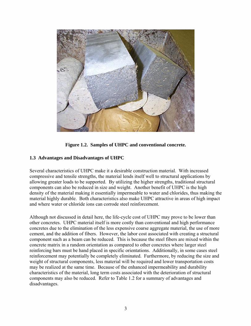
The constitutive properties of UHPC in tension are difficult to quantify with research still investigating this issue and with different researchers formulating slightly different conclusions. Graybeal and Hartmann [1] determined the cracking strength of UHPC using different methods, agreeing fairly well with other researchers, as shown in Table 2.3 for three different tensile tests and for four different curing conditions. Chuang and Ulm [2] attempted to define the tensile constitutive properties of UHPC as shown in Fig. 2.3 using a notched tensile plate test. However, the stress-strain relationship is not fully defined because results are not provided beyond the peak stress. The AFGC [3] also defined the tensile properties of UHPC. However, the recommendations require arbitrary determinations in order to obtain a complete stress-strain curve.
Table 2.3. Tensile cracking strength of UHPC tested by Graybeal and Hartmann [1].
Curing Method Mortar Briquette (ksi) Split Cylinder (ksi) Direct Tension (ksi)Steam 1.20 1.70 1.60
Air 0.90 1.30 0.82Tempered Steam 1.45 1.60 1.14Delayed Steam 1.00 1.60 1.62
10
-2.0
-1.5
-1.0
-0.5
0.0
-5 -4 -3 -2 -1 0
Strain (10-3
)
Stre
ss (k
si)
Figure 2.3. Tensile constitutive properties of UHPC reported by Chuang and Ulm [2].
Some research has suggested limiting flexural tensile strain based on the height of the specimen undergoing flexural loads. The reason for limiting the strain is because as the crack width grows large in comparison to the length of the fibers, it is postulated that tension stresses will not be transferred across the crack. Gowripalan and Gilbert [5] have proposed a limiting strain value shown in equation 2.1. The AFGC [3] recommends a similar limiting strain value shown in equation 2.2.
l = d
L f
2.1 001.0 strain limit (2.1)
Where: fL = length of fibers (in.)
d = depth (in.)
l = H
L f
8
3 strain limit (2.2)
Where: H = height of specimen (in.) Research has also been conducted at ISU separate from the work summarized herein by Bristow and Sritharan [4]. In that work, direct tension tests using dog-bone-shaped samples were conducted to determine the constitutive tensile properties of UHPC. The properties established in that work matched relatively well with the properties determined by Chuang and Ulm [2]. However, Bristow and Sritharan’s results are extended to a larger strain level. Figure 2.2 shows the stress-strain relationship as linear to a stress of 1.3 ksi at which point the stress increases to 1.7 ksi, flattens off and then declines gradually.

11
2.2 Flexural Strength
Previous research by Park, Chuang and Ulm [6] and Ulm and Chuang [7] has been completed concerning the flexural capacity of an UHPC member. Equations 2.3 through 2.13 summarized below were proposed by the authors to ensure that a given section is acceptable under given loading conditions.
Tc = c
pc
A
A prestressing ratio (2.3)
Where: pcA = area of strands within bottom flange (in.2)
cA = area of bottom flange (in.2)
= pup
f
fA
P
final prestressing percentage (2.4)
Where: fP = prestressing force final (kips)
pA = area of strands (in.2)
p = Tpu cf prestressing equivalent external pressure (ksi) (2.5)
l =
200
3,
8
3max
H
L f strain limit (2.6)
csE = cfpTcf EEcE modulus of composite concrete and strands (ksi) (2.7)
csf =
cr
c
csl
c
cscspuT f
E
E
E
EMEffcf 11,1min maxmax
maximum stress of composite concrete and strands (ksi) (2.8)
Where: M = applied external moment (in.- kips)
j = ccs Afpd
M
)( lever arm percentage of depth (2.9)
iM = djApM c internal moment (in.- kips) (2.10)
cF = dj
M i
compressive force (kips) (2.11)
cf = t
c
A
F compressive stress (ksi) (2.12)
Where: tA = area of top flange (in.2)
cf < cf ` (2.13)

12
2.3 Shear Strength
One simple procedure to compute an estimated ultimate shear strength of an UHPC structure has been developed by Chuang and Ulm [7] using previous information from the AFGC [3] as shown in equations 2.14 through 2.16. The basic concept of this procedure is to simply add the concrete contribution and fiber contribution to determine an ultimate shear strength. In this formulation, the concrete shear strength is determined empirically as the square root of the compressive strength. The fiber contribution is determined based on the tensile strength acting perpendicular to a crack. The crack occurs over the moment arm height and the web width. The height of the moment arm is estimated to be 90% of the depth. The tangent term is derived by finding the vertical component of the tensile strength that acts over the diagonal length of the crack. A partial safety factor is used to account for the degree to which the strength of this new material is still unknown. It should be pointed out that this procedure does not provide any information about the response of the structure.
cV = cw fdb `7.1 concrete shear contribution (kips) (2.14)
Where: wb = width of web (in.)
d = depth (in.)
fV = tan
9.0 max
bf
w fdb fiber shear contribution (kips) (2.15)
Where: bf = partial safety factor = 1.3
= crack angle (degrees)
nV = fc VV nominal shear strength (kips) (2.16)
Research has been completed by Padmarajaiah and Ramaswamy [8] using a truss model to determine shear capacity for high strength fiber reinforced concrete. In addition, strut and tie models [9], [10] and plasticity models [10] have been used by many different individuals to determine shear capacity of conventional concrete. Once again, these procedures do not provide information about the expected behavior of the structure.
The main advantage of using a strut and tie model is that it enables analysis and design of regions in a structure that do not satisfy the assumption that plane sections remain plane. This assumption may not be true for regions with discontinuities in loading or geometry. St. Venant’s Principle states that the D-region extends a distance away from a discontinuity equal to the overall height of the member.
When designing using a strut and tie model, a truss model should be created. This model should include struts where compression forces are expected, ties where tensile forces are expected, and nodes at the intersection of the struts and ties. Figure 2.4 demonstrates a possible truss model for a simply supported deep beam loaded with a concentrated load. Several different truss models

13
may be possible for a single structure, but each will be acceptable if the following procedures are followed. The determination of the geometry of the truss may be somewhat iterative. Once the truss model is developed, the forces in each of the nodes, struts, and ties should be determined. The design strength of each component should be greater than the applied loads. According to the American Concrete Institute (ACI) code [9], the design strength is found by multiplying the nominal strength by a strength reduction factor of 0.75.
node
node
struts tie
Figure 2.4. General strut and tie truss model.
The nodes should be examined to ensure sufficient strength. The nodes rely on compression of the concrete to resist the forces of the struts and ties. The nominal compression strength at the face of a nodal zone defined by ACI is reproduced in equation 2.17. The node factor is 1.0, 0.8, or 0.6 for a node with no ties, one tie, or two ties respectively. If one is examining a two dimensional structure, the area of the nodal face may be determined by using the width of the member in one direction. The size of the node in the other direction should be increased until the design strength is equal to or greater than the applied force. At this point iteration may take place if the change in size of the nodes affects the geometry of the truss model.
nnF = ncn Af `85.0 nominal nodal force (kips) (2.17)
Where: n = node factor
nA = area of nodal face (in.2)
The strength of the struts should be examined to ensure sufficient strength. ACI has determined the nominal compressive strength of the strut according to equation 2.18. The strut factor is 1.0 for struts with uniform cross section, 0.75 for bottle-shaped struts with adequate reinforcement, 0.4 for struts passing through cracks of a tensile zone, and conservatively 0.6 for struts within beam webs where struts are likely to be crossed by inclined cracks. The area of the strut should equate to the area of its nodal face.
nsF = stcst Af `85.0 nominal strut force (kips) (2.18)
Where: st = strut factor
stA = area of strut (in.2)

14
The strength of the ties should be adequate for design. ACI has determined the nominal strength according to equation 2.19. Included is strength from mild reinforcement and prestressing strands.
ntF = ppys fAfA nominal tie force (kips) (2.19)
Where: sA = area of mild reinforcement (in.2)
yf = yield strength of mild steel reinforcement (ksi)
pA = area of strands (in.2)
pf = stress in strand (ksi)
ACI also has recommendations for the amount of transverse reinforcement to be used. In addition, anchorage of the ties is discussed. Refer to the reference [9] for further information.
There are four major models that have been developed for conventional reinforced concrete that can predict both capacity and response of an element under shear or combined flexure and shear. They are the compression field theory (CFT) [11], the MCFT [11], the rotating angle softened truss model (RASTM) [10], and the fixed angle softened truss model (FASTM) [10]. The basic idea of each of the approaches is to be able to predict the capacity and response of an element by using equations of equilibrium, equations of compatibility, and constitutive stress-strain relationships of concrete compression, concrete tension, and reinforcement.
The models have some unique characteristics that differentiate them from one another. The CFT assumes that after cracking, no tensile stress is carried by the concrete across cracks; this is generally an overly conservative assumption. The MCFT accounts for a realistic concrete tensile stress after cracking. The compression field theories provide information on how to apply the models in a simplified sectional approach to analysis. The truss models, however, are designed more for a finite element analysis. The specific difference between the two truss models is that the FASTM assumes that the final angle of the principal compressive stress coincides with the angle of the initial cracks while a rotating angle is assumed for the RASTM (and the compression field models). A rotating angle means that the angle of the principal compressive stress increases as the ratio of applied shear to moment increases. In addition, the FASTM introduces another constitutive relationship between shear stress and shear strain.
The MCFT is the model that will principally be used for this research. Application of the MCFT for analytical modeling of UHPC beams is described in Chapter 5 based upon fundamentals of the MCFT as described by Collins and Mitchell [11]. In addition, Chapter 7 recommends a shear design procedure using the MCFT approach coupled with equations 2.14 through 2.16. Equations 2.20 through 2.41 and related descriptions are from Collins and Mitchell [11], describing the MCFT analytical procedure for use with conventional concrete with stirrups. The solution process is carried out at the mid-height of the web using the following steps:
1. Choose a value of the principal tensile strain at which to perform the calculations.

15
2. Estimate the principal compressive stress angle. 3. Calculate the crack width using equation 2.25. 4. Estimate the shear reinforcement stress. 5. Calculate the principal tensile stress using equation 2.28. 6. Calculate the shear force using equation 2.32. 7. Calculate the principal compressive stress using equation 2.30. 8. Calculate the maximum principal compressive stress using equation 2.34. 9. Ensure that the principal compressive stress is less than the maximum principal
compressive stress. If this is not satisfied, return to step 1 and decrease the magnitude of the principal tensile strain.
10. Calculate the principal compressive strain from equation 2.35. 11. Calculate the longitudinal and vertical strains from equations 2.36 and 2.37. 12. Calculate the shear reinforcement stress from equation 2.38. 13. Ensure that the estimated shear reinforcement stress from step 4 is near the stress
calculated in step 12. If not, then return to step 4 and make a new estimate. 14. Calculate the stresses in the longitudinal mild steel reinforcement and prestressing
strands using equations 2.39 and 2.40, respectively. 15. Calculate the axial force on the member using equation 2.43. 16. Ensure that the calculated axial load is equivalent to the applied axial load. If the
calculated axial load is more tensile than the applied, then return to step 2 and increase the value of the principal compressive stress angle.
17. Ensure that equation 2.44 is satisfied. If not, the principal tensile stress from step 5 needs to be incrementally reduced in magnitude.
18. Calculate the sectional curvature based on a plane sections analysis (strain compatibility) using the calculated longitudinal strain from step 11.
19. To obtain the complete response of the beam, these calculations are repeated for a range of values for the principal tensile strain.
The crack spacing parameters are used to determine the crack width as suggested by the MCFT in equations 2.20 through 2.25. Equations 2.22, 2.23, and 2.26 are not applicable for UHPC. Development of such equations for UHPC should be investigated by future research.
x = A
AA ps longitudinal reinforcement ratio (2.20)
Where: sA = area of mild reinforcement (in.2)
pA = area of strands (in.2)
A = gross cross-sectional area of member (in.2)
v = sb
A
w
v
shear reinforcement ratio (2.21)
Where: vA = area of shear reinforcement within distance s (in.2)
wb = width of web (in.)
s = spacing of shear reinforcement (in.)

16
mxs = x
bxxx
dk
sc
125.0
102 crack spacing in longitudinal direction (in.) (2.22)
Where: xc = maximum distance from longitudinal reinforcement in vertical direction (in.)
xs = spacing of longitudinal reinforcement in transverse direction (in.)
1k = 0.4 for deformed bars and 0.8 for plain bars or bonded strands
bxd = diameter of longitudinal reinforcement (in.)
mvs = v
bvv
dk
sc
125.0
102 crack spacing in vertical direction (in.) (2.23)
Where: vc = maximum distance from shear reinforcement in transverse direction (in.)
bvd = diameter of shear reinforcement (in.)
ms =
mvmx ss
cossin1
crack spacing in direction of principal compressive stress (in.) (2.24)
w = mp s1 crack width (in.) (2.25)
The shear stress along a crack can be determined by the use of equation 2.26 as suggested by the MCFT based on empirical data. It can be seen that stronger concrete, smaller crack width, and larger aggregate all contribute to a higher shear stress along a crack. This shear stress will be used as one condition for finding the principal tensile stress.
ci =
63.0
243.0
`16.2
a
w
f c shear stress at crack (ksi) (2.26)
Where: a = maximum aggregate diameter (in.) A second condition for finding the principal tensile stress is derived by using the calculated average stresses and the local stresses at a crack as shown in Fig. 2.5. The vertical force in the two stress states must be equivalent as described in equation 2.27 in order for the average stresses to accurately model the local conditions. Keep in mind that tensile stresses are negative values, while compression and shear stresses are positive values. Also note that the lever arm is the distance from the tensile force resultant to the compressive force resultant. If the crack width has become large enough that the shear stress across the crack is reduced significantly, equation 2.27 can be solved to find the principal tensile stress. This is shown in the first term of equation 2.28. If the crack width has not become large, the principal tensile stress is determined through an empirical procedure developed by the MCFT and described in the second term of equation 2.28.

17
p1
Av fv
jd
s s
jdci
vyfvA
a. Calculated average stresses. b. Local stresses at crack.
Figure 2.5. Average and local stresses transmitted across cracks used by the MCFT [5].
sintan 1
djb
s
djfA w
pvv
= djbs
djfA wcivyv
tan
(2.27)
1p =
1
21
5001,tanmin
p
crcivvy
w
v fff
bs
A
principal tensile stress (ksi) (2.28)
Where: 1 = 1.0 for deformed, 0.7 for plain, and 0 for unbonded reinforcement
2 = 1.0 for short-term monotonic loading and 0.7 for sustained and/or repeated loads
crf = cracking tensile strength of concrete (ksi)
vyf = yield strength of shear reinforcement (ksi)
The MCFT assumes a simple shear stress distribution constant over the depth of the moment arm as given in equation 2.29.
xy = djb
V
w shear stress in the x-y plane (ksi) (2.29)
Using Mohr’s circle of average stresses shown in Fig. 2.6, the principal compressive stress can be developed as shown in equation 2.30.

18
xy
x
y
normalstress
p2p1
2
shearstress
Figure 2.6. Mohr’s circle of average concrete stresses in a general concrete element [5].
2p = 1cottan pxy principal compressive stress (ksi) (2.30)
The principal compressive stress within a concrete member tends to push apart the top and bottom of the member while the principal tensile stress and the shear reinforcement pull the two back together. This requires a state of equilibrium in the vertical direction that is demonstrated in Fig. 2.7 and equation 2.31. When equations 2.29, 2.30, and 2.31 are combined and mathematically rearranged, equation 2.32 can be derived, describing the applied shear force.
vv fA = sbwpp 21
22 cossin (2.31)
V = cotcot1
djs
fAdjb vv
wp applied shear (kips) (2.32)
Two factors that influence the calculation of principal compressive strain are the principal compressive stress and the principal tensile strain. It is obvious that the principal compressive stress is interdependent on the principal compressive strain because each is assumed to be oriented in the same direction in MFCT. Typically, the relation of this stress and strain in a uniaxial orientation would be described by the modulus of elasticity. The MCFT has described a parabolic relation between the compressive stress and strain given in equation 2.33 that is more accurate than a straight line. However, because there is a biaxial state of stress, the same relation does not apply. In a biaxial state of stress, when a tensile strain is applied in the out-of-plane direction, the concrete will have a lower compressive strength in the in-plane direction. This

19
relationship is described in equation 2.34. Therefore, by substituting the maximum principal compressive stress from equation 2.34 for the compressive strength in equation 2.33 and then solving for the principal compressive strain, equation 2.35 is derived.
2p =
2
22
``2`
c
p
c
pcf
principal compressive stress (ksi) (2.33)
mp2 11708.0
`
p
cf
cf ` maximum principal compressive stress (ksi) (2.34)
2p =
mp
pc
2
211`
principal compressive strain (2.35)
Where: c̀ = strain associated with cf `
s
p1 p2
vfvA
Figure 2.7. Vertical forces used in MCFT equilibrium condition.
The longitudinal and vertical strains can now be calculated as given in equations 2.36 and 2.37 based on Mohr’s circle of average strains from Fig. 2.8.

20
x
normalstrain
2
shearstrain
p2 p1
y
2
xy2
Figure 2.8. Mohr’s circle of average concrete strains in a general concrete element [5].
x =
2
22
1
tan1
tan
pp longitudinal strain (2.36)
y =
2
12
2
tan1
tan
pp vertical strain (2.37)
Using these calculated strains, the stresses in the shear reinforcement, longitudinal mild reinforcement and the longitudinal prestressing strands can be calculated as described in equations 2.38 to 2.40.
vf = ysE vyf stress in shear reinforcement (ksi) (2.38)
Where: sE = modulus of mild reinforcement (ksi)
sf = xsE yf stress in mild reinforcement (ksi) (2.39)
Where: yf = yield strength of mild reinforcement (ksi)
pf =
pp
fxp EA
PE pyf stress in strand (ksi) (2.40)
Where: pyf = yield strength of strand (ksi)

21
The axial force in the member is dependent on the forces in the longitudinal reinforcement, the shear force, the stresses within the web, and the longitudinal stresses outside the web. The longitudinal stresses outside the web are only needed for compression because tension is negligible in conventional concrete. This compressive stress is described in equations 2.41 and 2.42. Then the axial force can be calculated using equation 2.43.
If x 0 then,
cf = 0 compressive stress (ksi) (2.41)
If x 0 then,
cf =
2
``2`
c
x
c
xcf
compressive stress (ksi) (2.42)
N = djbAfdjbVfAfA wccwpppss 1cot axial force (kips) (2.43)
In order for the previous analysis to be correct, the longitudinal reinforcement must not fail at the location of a crack and the resultant horizontal force based on the calculated average stresses and local stresses shown in Fig. 2.5 must be equivalent. This holds true if equation 2.44 is satisfied.
pspys fAfA djbfAfA wpppss 1
21 cot
djbff
sb
Awvvy
w
vp (2.44)
Where: psf = stress in strand at nominal strength [9] (ksi)
Collins and Mitchell [11] also suggest a shear design procedure for use with conventional concrete with stirrups. It is assumed that the section has already been designed based on flexure. The shear stirrups can be designed by using the following steps outlining the shear design procedure.
1. Calculate the shear stress ratio using equation 2.45. 2. Ensure that the shear stress ratio is less than 0.25. If this is not satisfied, increase the
size of the section or the concrete strength. 3. Estimate the principal compressive stress angle. 4. Calculate the longitudinal strain using equation 2.46. 5. Determine θ and β using Table 2.4. 6. Ensure that the estimated principal compressive stress angle from step 3 is near the
calculated value from step 5. If not, then return to step 3 and make a new estimate. 7. Calculate the concrete shear contribution using equation 2.47. 8. Calculate the reinforcement shear contribution using equation 2.48. 9. Determine the shear reinforcement spacing based on equation 2.49. 10. Ensure that yielding of the longitudinal reinforcement does not occur by satifying

22
equation 2.50. If needed, either add more longitudinal reinforcement or revise the values of θ and β using the values for a higher longitudinal strain. These values will reduce the amount of longitudinal reinforcement but increase the amount of stirrups required.
To begin the design, the shear stress ratio and the longitudinal strain should be determined. The shear stress as earlier described is assumed to be constant over the moment arm length as shown in equation 2.45. The longitudinal strain in reinforcement can be described by prestressing, flexural, shear, and axial forces converted to stress using the area of reinforcement and then converted to strain using the modulus of elasticity as described by equation 2.46. This strain is also the strain within the concrete assuming no slip between the concrete and reinforcement.
c
xy
f `
=
djbf
VV
wc
pu
` shear stress ratio (2.45)
Where: uV = factored ultimate shear force (kips)
pV = shear force provided by strands (kips)
x = ppss
uuu
f
AEAE
NVdj
MP
5.0cot5.0 longitudinal strain (2.46)
Where: uM = factored ultimate moment (in.- kips)
uN = factored ultimate axial force (kips)
Using the calculated value of the longitudinal strain, the two factors defined below are determined using empirical data described by Table 2.4. The shear strength contribution of concrete then can be found using equation 2.47.
cV = djbf wc ' concrete shear contribution (kips) (2.47)
Where: = tensile stress factor = principal compressive stress angle (degrees) The reinforcement shear contribution is found using equation 2.48 assuming that the design shear strength is equivalent to the applied factored shear force. The required spacing of shear reinforcement then can be described by equation 2.49.
sV = cpu VV
V
reinforcement shear contribution (kips) (2.48)
Where: = strength reduction factor
s s
yv
V
djfA cot spacing of shear reinforcement (in.) (2.49)

23
Table 2.4. MCFT shear design factors for concrete members with web reinforcement [11].
ShearStressRatio 0 -0.25 -0.50 -0.75 -1.00 -1.50 -2.00 -2.50 -3.00 -5.00
θ (deg.) 28 31 34 36 38 41 43 45 46 56β 5.24 3.70 3.01 2.62 2.33 1.95 1.72 1.54 1.39 0.92
θ (deg.) 28 30 30 34 36 40 42 43 43 56β 4.86 3.37 2.48 2.37 2.15 1.90 1.65 1.44 1.25 0.92
θ (deg.) 22 26 30 34 36 38 38 38 38 55β 2.71 2.42 2.31 2.27 2.08 1.72 1.39 1.16 1.00 0.95
θ (deg.) 23 27 31 34 36 36 36 36 36 55β 2.40 2.33 2.29 2.16 2.00 1.52 1.23 1.03 0.88 0.94
θ (deg.) 25 28 31 34 34 34 34 34 35 55β 2.53 2.25 2.13 2.06 1.73 1.30 1.04 0.85 0.77 0.94
θ (deg.) 26 29 32 32 32 32 34 36 38 54β 2.34 2.19 2.11 1.69 1.40 1.01 0.94 0.91 0.88 0.96
θ (deg.) 27 30 33 34 34 34 37 39 41 53β 2.16 2.13 2.09 1.82 1.52 1.08 1.11 1.04 0.99 0.98
θ (deg.) 28 31 34 34 34 37 39 42 44 -β 1.97 2.07 2.08 1.67 1.35 1.29 1.17 1.16 1.09 -
θ (deg.) 30 32 34 35 36 39 42 45 49 -β 2.26 2.00 1.87 1.63 1.45 1.37 1.32 1.28 1.24 -
0.250
0.125
0.150
0.175
0.200
0.225
Longitudinal Strain εx x 1000
< 0.050
0.075
0.100
The longitudinal reinforcement should be examined to avoid yielding. By considering all of the forces on the member, the longitudinal reinforcement will not yield if equation 2.50 is satisfied.
pspys fAfA
cot5.05.0
ps
uuu VVV
dj
MN (2.50)
Where: psf = stress in strand at nominal strength [9] (ksi)
2.4 Structural Testing
Structural testing of a UHPC beam was completed at the FHWA Turner Fairbanks Highway Research Center (TFHRC) Structural Engineering Laboratory. Flexural and shear testing procedures, instrumentation, and results have been described by Park, Chuang, and Ulm [6] and by Chuang and Ulm [12]. The test configurations are shown in Figs. 2.9 and 2.10. The tested beam was an AASHTO type II girder made of UHPC and is shown in Fig. 2.11. The Flexure Test was first performed on this beam resulting in a failure of the beam at midspan where the entire two halves of the beam separated. The Shear Test #1 and Shear Test #2 then took place on the broken portions of the original beam. Refer to Figs. 5.17 and 5.18 for some of the results of this testing.

24
435"9" 72" 435" 9"
a. Flexure Test
48"90"198"144"72" 6"96"6"
b. Shear Test #1 c. Shear Test #2
Figure 2.9. FHWA flexure and shear testing setup diagrams.
Figure 2.10. FHWA flexure test setup photograph.
2.5 Prestress Bond
The bond between prestressing strands and UHPC has been investigated by Lubbers [13] using a pullout test with 0.5 in. strands and 0.5 in. oversized strands embedded within UHPC specimens that were 12 to 24 in. deep using the test setup shown in Fig. 2.12. The strands had no prestressing force applied and were spaced at 9 in. within the test specimen. Conclusions were drawn that the development length of 0.5 in. strands within UHPC is greater than 18 in. but less than 24 in. and is approximately 12 in. for the 0.5 in. oversized strands. This was based on the depth of the specimen required to cause fracturing of the strands without slipping.

25
6"
6"
6"
15"
6"
3"
18"
12"
36"
* 12" strands spaced at 2"
Figure 2.11. Prismatic cross section of AASHTO type II FHWA test beam.
LVDT
Chair
LVDT
Prestressing Strand
Spacers
Load Cell
Hydraulic Cylinder
Test Specimen
Prestressing Chuck
12" Variable 48"
Figure 2.12. Pull-out test apparatus used by Lubbers [13].
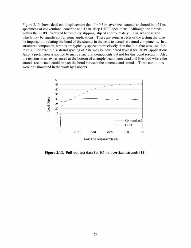
26
Figure 2.13 shows dead end displacement data for 0.5 in. oversized strands anchored into 24 in. specimens of conventional concrete and 12 in. deep UHPC specimens. Although the strands within the UHPC fractured before fully slipping, slip of approximately 0.1 in. was observed which may be significant for some applications. There are some aspects of the testing that may be important to relating the bond of the strands in the tests to actual structural components. In a structural component, strands are typically spaced more closely than the 9 in. that was used for testing. For example, a strand spacing of 2 in. may be considered typical for UHPC applications. Also, a pretension is applied to many structural components but not for this bond research. Also, the tension stress experienced at the bottom of a simple beam from dead and live load where the strands are located could impact the bond between the concrete and strands. These conditions were not simulated in the work by Lubbers.
0
5
10
15
20
25
30
35
40
45
50
0 0.02 0.04 0.06 0.08 0.1
Dead End Displacement (in.)
Loa
d (k
ips)
Conventional
UHPC
Figure 2.13. Pull-out test data for 0.5 in. oversized strands [13].

27
CHAPTER 3: FIELD BRIDGE DESCIPTION
The first UHPC bridge in the United States was constructed in Wapello County, Iowa during the fall of 2005. The bridge has no horizontal curve, vertical curve, nor skew. The cross section of the bridge as a whole is shown in Fig. 3.1. The deck has a 2% transverse crown from the peak at the centerline of the roadway. The deck reinforcement consists of transverse and longitudinal steel in both the top and bottom of the deck. The transverse steel has top cover of 2.5 in. and bottom cover of 1 in. with the longitudinal steel placed inside of the transverse steel. The #7 transverse bars are spaced at 9 in. across the width of the deck in both the top and bottom of the slab. In addition, #5 transverse bars spaced at 9 in. between the #7’s are in the top of the deck in the outer 6.67 ft of the deck to further strengthen the overhang. The longitudinal steel consists of #5 bars spaced at 1 ft between the beams, with the top and bottom reinforcement staggered in spacing. Similar reinforcement exists in the overhang of the deck. There is one diaphragm located at midspan of the bridge consisting of two C15x33.9 steel sections with one connecting each of the outer beams to the center beam at the mid-depth of the beams. Conventional Iowa DOT integral abutments with wingwalls and open guard rails were used for this bridge.
115" 115"
294"
326"
8.5"8" 9"#7 Transverse#5 Longitudinal
#5
Figure 3.1. Cross section of Wapello County UHPC bridge.
The three bridge beams used on this project were modified slightly from the Iowa DOT Bulb Tee C standard with the dimensions shown in Fig. 3.2. The beams are 111 ft long with a 110 ft span. Note the solid five strands that are aligned vertically near the top of Fig. 3.2.a. These are the harped stands that decline linearly from the end cross section (Fig. 3.2.a.) to the midspan cross section (Fig. 3.2.b.) over a distance of 44.5 ft as shown in Fig 3.3. Within the central 22 ft of the beam, all the strands run horizontally and are located as shown in the midspan cross section. There are #5 reinforcing bars with two legs in the top of the bridge beams in order to connect the deck and beams for composite action and resist horizontal shear. The spacing of the horizontal shear bars are shown in Fig. 3.3. The last 3.5 ft of the beams on both ends have eight strands that are debonded in the bottom flange. The last 6.5 ft of the beams on both ends have 16 strands that are debonded in the bottom flange. Debonding was used in order to reduce the stresses at the flange-web interface. No shear reinforcement is present within the beams.

28
42.00"
26.50"
32.00"
28.00"
R=8.00"
R=8.00"
0.75" Chamfer
4.50"
5.50"
5.50"
2.81"1.69"
R=2.00"R=2.00"
1.69"2.81"
5.50"
5.50"
4.50"
0.6" strands spaced at 2 in.
0.75" Chamfer
R=8.00"
R=8.00"
28.00"
32.00"
26.50"
42.00"
0.6" strands spaced at 2 in.
a. End cross section. b. Midspan cross section.
Figure 3.2. Cross sections of Wapello County UHPC bridge beams.
Harped Strands
Centerline
8-12" 6-15" 17-18"
132"534"
Spacing of #5 Horizontal Shear Bars
1-9" 13-9"8-6"
Figure 3.3. Elevation of Wapello County UHPC bridge beams.
3.1 Design
Design of the bridge was completed cooperatively between the Iowa DOT, Wapello County, and ISU. Initially, a global grillage analysis was completed for determination of accurate shear and moment distribution factors for the individual beams. As no U.S. specification existed for UHPC design, the design of the beams for flexural capacity was completed using two different approaches. The procedure which will be described in section 5.2.1 was used and checked using

29
conventional design assumptions (e.g., no tension in the concrete, a typical Whitney Stress Block, etc.) Composite action between the slab and the beams was considered. Shear design was completed using equations 2.14 through 2.16. In addition, full-scale shear testing as described in section 4.2 was completed before construction of the bridge to verify all design assumptions.
3.2 Construction
Each of the bridge beams was cast on separate days of June 25th, July 9th, and July 16th, 2005 at a concrete plant in Winnipeg, Manitoba, Canada. The construction procedure used with UHPC is somewhat atypical of conventional concrete with some important differences in the preparation, mixing, placing, and curing.
Preparation of the beams began by pulling the prestressing strands through the end formwork and stressing them between abutments to the appropriate level. Next, the side formwork was placed after being greased. Bolted struts were used to hold the formwork together transversely. One of the differences of UHPC from conventional concrete is its liquidity, requiring that the formwork must be specifically prepared to prevent leaking or lifting. In this instance, all joints and prestressing holes of the formwork were sealed with putty. UHPC tends to apply high hydrostatic pressures to portions of the formwork that are “above” the concrete (such as the taper of a bottom flange). Therefore, the formwork was fastened to the ground to prevent lifting of the forms.
Batching of the concrete took place in a four motor pan mixer with a 2.6 cubic yard capacity, capable of 50 rpm. Mixing UHPC requires special specifications as compared to conventional concrete. For instance, the mixer needs to input high amounts of shear, have minimum blade clearances, be capable of variable speed, and contain an amp meter. For casting of the UHPC bridge beams, batches of 1.3 cubic yards were mixed. First, the prepackaged bags of Ductal® were emptied into the mixer. As the mixer began at low power, the water and the first portion of the admixture were added. Since the temperature was quite high during mixing, a portion of water was replaced with ice. As the power was increased, the rest of the admixture was added and the mixing continued. Then as the power was decreased, the steel fibers were slowly introduced. Additional mixing occurred until the UHPC was ready to be placed. For this project more concrete was needed than could be mixed at once. Therefore, several batches of concrete were mixed and held in two ready mix trucks which continually agitated the fluid concrete.
Placement of the concrete occurred from only one end of the beam. If this is not done, a joint or lense may form where separate concrete pours come together. In this case, placement was completed by placing concrete directly from the ready mix trucks into one end of the formwork as shown in Fig. 3.4. As the formwork filled, the truck was slowly moved along the length of the beam so that no overflow occurred. However, in this situation care was taken to ensure that the concrete was always placed on flowing concrete, not placed into an area of the formwork where no concrete was present. Tools like shovels and two-by-fours were used to push the surface concrete into depressed areas of the form. This was only to fill the forms as the concrete should never be troweled because it causes too much moisture to rise to the surface. At this point,

30
inverted U-shaped mild reinforcement was installed in order to provide horizontal shear reinforcement between the beams and the bridge deck.
Figure 3.4. Placement of concrete during construction of Wapello County UHPC bridge beams.
In order to initiate the curing process and also to reduce shrinkage, the beams were tightly sealed. This was done by spraying a sealing chemical on the top surface of the freshly placed concrete. Tarps were then placed over the entire assembly to hold in moisture and heat during steam curing which was conducted for 12 hours at 140 °F. Once the concrete reached the specified strength, in this case 12 ksi as determined by cylinder testing, the strands were released. To release the strands, heat was applied with an acetylene torch, causing the strands to slowly elongate and lose stress. Following release, the UHPC was heat treated at 194 °F for a period of 48 hours.
These beams were then shipped to the bridge site where conventional concrete abutments had been previously constructed. Casting of the bridge deck took place on November 8th, 2005 with conventional concrete and normal construction practices. Additional construction of the guard rails, approach slab and grading of dirt took place on site in Wapello County, Iowa through the fall of 2005 with the nearly completed bridge shown in Fig. 3.5.

31
Figure 3.5. Elevation of Wapello County UHPC bridge.


33
CHAPTER 4: EXPERIMENTAL TEST PROGRAM
This chapter summarizes the experimental test program and consists of descriptions of the test specimens, setups, and procedures. Subsequently in Chapter 6, observations and results are discussed.
4.1 Material Testing
4.1.1 Uniaxial Compression Testing
Uniaxial compression tests on cubes were used to determine the compressive strength of the UHPC utilized in this study. Cubes were chosen instead of cylinders because the rough top surface created from casting of the concrete can be placed to the side, leaving flat, parallel surfaces on the top and bottom.
4.1.1.1 Test Specimen Description
Concrete cubes were cast on four different days when a beam was also constructed as follows: 42 specimens were cast on February 23rd, 2005, six specimens on June 25th, 2005, six specimens on July 9th, 2005, and nine specimens on July 16th, 2005. There were three different types of curing conditions applied to the cubes. Out of the 42 specimen cast during February, seven were cured with the beam, 14 were cured in a 194°F chamber, and 21 were cured at room temperature which was approximately 65°F. All of the cubes cast during June and July were cured with their respective UHPC beams. The cubes all had a side length of 1.97 in.
4.1.1.2 Test Configuration
Compression testing was completed following the provisions of ASTM C-109 [14]. The test was setup by placing the cube between a piece of steel and the test machine head as shown in Fig. 4.1.
4.1.1.3 Test Procedure
The test machine recorded the load and displacement of the table head throughout each test. The concrete cubes were tested at a loading rate of 300 lbs/sec. A rate above the ASTM C-109 [14] standard was required due to time constraints. A high compressive strength causes a long test duration unless the loading rate is increased.

34
Figure 4.1. Uniaxial compression test setup used for UHPC cubes.
4.1.2 Prism Flexural Testing
Flexural tests on prisms were used to determine the cracking strength of UHPC following the guidelines of ASTM C-78 [14]. This procedure was developed for testing conventional concrete, which, when unreinforced, fails at a load referred to as the cracking load. However, the same is not true of UHPC due to the presence of fibers; therefore in this work, the cracking load was defined as the point where load and displacement were no longer linear.
4.1.2.1 Test Specimen Description
UHPC prisms were cast on four different days when a beam was also constructed as follows: 42 specimens were cast on February 23rd, 2005, 12 specimens on June 25th, 2005, 12 specimens on July 9th, 2005, and 12 specimens on July 16th, 2005. There were three different types of curing conditions applied to the cubes. Out of the 42 specimen cast during February, seven were cured with the beam, 14 were cured in a 194°F chamber, and 21 were cured at room temperature which was approximately 65°F. All of the cubes cast during June and July were cured with their respective beams. The concrete prisms had dimensions of 1.57 in. x 1.57 in. x 6.30 in.
4.1.2.2 Test Configuration
The flexure testing was completed according to the provisions of ASTM C-78 [14]. The prisms were setup in a material test machine head using a span length of 4.5 in. with two load points spaced 1.5 in. apart and centered within the span as shown in Fig. 4.2.

35
Figure 4.2. Flexure test setup used for UHPC prisms.
4.1.2.3 Test Procedure
The test machine recorded the load and displacement of the table head throughout each test. The prisms were tested at a loading rate of 1,000 lbs/min as it was necessary to test at a higher rate than suggested by ASTM C-78 [14] in order to reduce the time required to complete each test.
4.2 Large-Scale Laboratory Testing
Large-scale laboratory testing was completed to collect information about the structural performance of UHPC girders. In all, three tests were conducted using one full-scale specimen. First, a flexure test provided information about the service limit state capacity of the beam and allowed the prestressing losses to be estimated. Next, a shear test provided information about the service and ultimate shear strength of the beam. And finally, a flexure-shear test permitted the service and ultimate shear strength of the beam to be determined when combined with significant applied moment.
4.2.1 Test Specimen Description
The cross sections of the large-scale laboratory test beam were the same as for the bridge beams shown in Fig. 3.2. The total length of the test beam was 71 ft with the harped strands varying linearly over a 28.5 ft long region at both ends of the girder. The central 14 ft of the beam had the midspan cross section shown in Fig. 3.2.b. Debonding was used in the same manner as previously described for the bridge beams.

36
4.2.1.1 Design
The test beam design was configured with the same cross section as the Wapello County, Iowa bridge beams and limited to a practical length and weight suitable for the ISU Structural Engineering Laboratory.
4.2.1.2 Construction
On February 23rd, 2005, the 71 ft long test beam was cast at a concrete plant in Winnipeg, Manitoba, Canada. The construction procedure was very similar to that described in section 3.2 with a few minor differences. As discussed previously, the UHPC mix tends to apply high hydrostatic pressures to portions of the formwork that are “above” the concrete such as the taper of a bottom flange. This pressure caused the laboratory beam formwork to lift up off its supports after the concrete was placed. Weight was added to the forms to push them back down at which point they were fastened to the ground to ensure that lifting did not occur again. The test beam was sealed using plastic sheets as opposed to the preferred chemical spray.
4.2.2 Flexural Testing
4.2.2.1 Test Configuration
The flexure test setup used in this work consisted of a 70-ft span with four applied point loads centered over the midspan, creating a constant moment region of approximately 64 in. Figures 4.3 and 4.4 show the test setup.
To quantify the response of the test beam, several different types of instrumentation were used and are shown in Figs. 4.5 and 4.6. The gage positions within each cross section are summarized in Table 4.1. During testing, a Megadac System and a Fiber Optic Interragator running at 1 Hz were used to collect data from the instruments including:
four load cells measuring loads (L1, L2, L3, L4) seven strain gage rosettes measuring strains in three directions (1, 2, 5, 6, 9, 13, 15) eight linear strain gages (3, 4, 7, 8, 10, 11, 12, 14) five fiber optic strain gages (F1, F2, F3, F4, F5) four DCDT’s measuring displacements between two points on the beam (H1, H2, H3,
H4) three DCDT’s measuring strand slip (S1, S2, S3) eight string potentiometers measuring deflection with a designation of “a” for those
placed on the north side of the beam, “b” for those placed on the south side of the beam, and no letter designation for those in the center of the beam (D1, D2, D3a, D3b, D4a, D4b, D5a, D5b)

37
22" 64" 22"L4 L3 L2 L1
366"366"6" 6"
Figure 4.3. Large-scale flexure test setup diagram.
Figure 4.4. Large-scale flexure test setup photograph.
#14
#13 #11
#12
F4F5
H1
H2
H4
H3
D5
210"6"
D4
210"
Figure 4.5. Instrumentation on east side for large-scale flexure test.

38
#8
#7
#2
#3
S3
S2
S1
#6,#15 on back #1#5#4
F1F3 F2#10
D1D2D3
20"66"78" 46" 6"
#9
Figure 4.6. Instrumentation on west side for large-scale flexure test.
Table 4.1. Location of strain gages used in large-scale flexure test.
GageVertical Position from Base (in.)
Horizontal Position from West Support (in.)
1 28 462 17 463 0 464 41 665 28 666 17 667 0 668 41 2109 17 210
10 0 21011 41 42012 0 42013 17 63014 0 63015 17 66H1 28 420H2 17 420H3 10.9 420H4 -1.875 420F1 2 66F2 2 132F3 2 210F4 2 420F5 2 630
4.2.2.2 Test Procedure
Flexural testing was performed on May 11th, 2005. Two sequences of loading were applied. During the first sequence of loading a total load of 237.4 kips was applied to the beam at which point the beam was inspected for flexural cracks at midspan. Additional loading was applied to

39
reach an approximate total load of 243 kips and 3 in. of midspan deflection. At this point, the beam was unloaded.
A second sequence of loading was then applied to the beam. The beam was first loaded to a total load of 256 kips and the beam was inspected for flexural cracks. Loading was resumed to a total load of 265 kips and 3.2 in. of deflection when the final inspection of the beam took place. Testing was halted at this point to maintain the structural integrity of the beam for the shear testing. It should be pointed out that the maximum applied moment is slightly under the service load condition and well under the ultimate load condition for the composite bridge beam and deck system.
4.2.3 Shear Testing
4.2.3.1 Test Configuration
The shear test setup was also configured to have a 70-ft span. The loading points were moved to the positions shown in Figs. 4.7 and 4.8. In order to reduce arching and deep beam action, a shear span to depth ratio of approximately 2.5 was used within the 90 in. region on the west end of the beam.
Nearly the same instrumentation used during the flexural testing was also utilized during the shear testing as shown in Figs. 4.9 and 4.10 with gages 1 through 15 and F1 through F5 unchanged and some small changes. The four DCDT’s (H1, H2, H3, H4) used as longitudinal strain gages at the midspan during the flexure test were moved to the end region and combined with two more for a total of six DCDT’s (R1a, R1b, R1c, R2a, R2b, R2c) essentially acting as two large-scale strain rosettes as shown in Fig. 4.11. These rosettes were located at a position 22.5 in. above the bottom of the beam.
4.2.3.2 Test Procedure
On June 9th, 2005 the shear test was performed. After total loads of 369.8 kips, 397.6 kips, and 594.0 kips were applied, the beam was inspected for cracks. Inspection took place at these loads due to audible cracking of the beam. The maximum total load applied during the test was 594.0 kips at which point the load began to decrease. Additional deflection was applied to the beam as the load decreased but is not significant to this research.
22"64"22"L1L2L3L4
6"6" 642" 90"
Figure 4.7. Large-scale shear test setup diagram.

40
Figure 4.8. Large-scale shear test setup photograph.
F5 F4
#12
#11#13
#14
210"
D4
6" 210"
D5
Figure 4.9. Instrumentation on east side for large-scale shear test.
#10 F2F3 F1
#4 #5 #1R2#6,#15 on backR1S1
S2
S3
#3
#2
#7
#8#9
D3 D2 D1
6"46"78" 66" 20"
Figure 4.10. Instrumentation on west side for large-scale shear test.

41
Figure 4.11. Large strain rosettes gages R1 and R2 used for large-scale shear test.
4.2.4 Flexure-Shear Testing
4.2.4.1 Test Configuration
This test was configured to have a 57-ft long span as shown in Figs. 4.12 and 4.13. The end region that was damaged during the shear test was allowed to overhang the support such as to minimize the influence on the behavior of the beam in this test. Two factors were balanced to determine an optimum loading position. The more the loads move toward the end of the beam, the more likely the beam is to fail in shear, but the less likely the moment will affect the shear strength. The selected configuration was thought to represent a typical combination of shear and bending loadings.
64"22"
36"210"6"
L1L2L3L4
352"
Figure 4.12. Large-scale flexure-shear test setup diagram.

42
Figure 4.13. Large-scale flexure-shear test setup photograph.
The instrumentation used for the flexure-shear test, shown in Figs. 4.14 through 4.16, was somewhat different than the previous two tests although gages 1 through 15 and F1 through F5 remain unchanged. The positions of gages not previously discussed are shown in Table 4.2. A Megadac System and a Fiber Optic Interragator running at 1 Hz were used to collect data from the instruments including:
four load cells measuring load (L1, L2, L3, L4) six strain gage rosettes measuring strain in three directions (9, 13, 15, 16, 17, 18) five linear strain gages (8, 10, 11, 12, 14) three fiber optic strain gages (F3, F4, F5) six DCDT’s essentially acting as two large-scale strain rosettes (R1a, R1b, R1c, R2a,
R2b, R2c) three DCDT’s measuring strand slip (S1, S2, S3) six string potentiometers measuring deflection with a designation of “a” for those
placed on the north side of the beam, “b” for those placed on the south side of the beam, and no letter designation for those in the center of the beam (D3a, D3b, D4a, D4b, D5a, D5b)
F5 #14#17#18
R2 R1#16 #13
S3
S2
S1
D5D6
6" 72" 74" 40"12" 12"
Figure 4.14. Instrumentation on east side for large-scale flexure-shear test.

43
#8#9
F3 #10
D4
#11
#12
F4
54"210" 163"
Figure 4.15. Instrumentation on west side for large-scale flexure-shear test.
Figure 4.16. Large strain rosette gage R1 used for large-scale flexure-shear test.
Table 4.2. Location of strain gages used in large-scale flexure-shear test.
GageVertical Position from Base (in.)
Horizontal Position from East Support (in.)
16 28 15817 17 15818 17 72R1 22.5 170R2 22.5 84

44
4.2.4.2 Test Procedure
On August 5th, 2005 the flexure-shear test was performed. A total load of 367 kips was applied and the beam was first inspected for cracking. Additional inspections took place at levels of 481.8 kips and at the maximum applied load of 658.1 kips. At this point the beam was suspected to have a slight amount of additional capacity. However, essentially no additional load was applied as the deflection increased to a maximum of about 8.5 in. at the easternmost load point. The test was then ended after the beam was unloaded.
4.3 Small-Scale Laboratory Testing
The purpose of the small-scale laboratory testing was to generate additional data on the shear behavior of UHPC under a variety of geometrical considerations. It was anticipated that analysis of the shear failure would provide a better definition of the shear strength of UHPC for use in design.
4.3.1 Test Specimen Description
Five different cross sections of small-scale beams, with three of each beam for a total of 15 beams were tested in the small-scale laboratory testing portion of this work. The different beams have different web widths, amount of reinforcement, and heights. The beam cross sections are shown in Fig. 4.17 with other important properties shown in Table 4.3. Sections A, B, and C in Fig. 4.17 have a height of 10 in. and will be collectively referred to as the 10-in. beams. Sections D and E in Fig. 4.17 have a height of 12 in. and will be referred to as the 12-in. beams.
2.00" 2.00"
8.00"
1.50"
2.00"
1.50"
2.00"
3.00"2.00"
8.00"
2.00" 2.00" 2.00" 2.00"
8.00" 8.00"
2.00"2.00"2.00"2.00"
8.00"
2.00"3.00"
2.00"
1.50"
2.00"
1.50"
8.00"
0.6"Dia.
0.5"Dia.
a. Section A. b. Section B.

45
Figure 4.17. Cross sections of small-scale test beams.
1.75"
8.00"
1.50"
3.00"2.00"
8.00"
2.00" 2.00" 2.00" 2.00"
8.00"
2.08"
1.33"
2.08"0.5"Dia.
c. Section C.
1.75" 1.50"
2.08"
2.08"
8.00"
2.00"2.00"2.00"2.00"
2.00"3.00"
1.50"
8.00"
3.33"10.00" 10.00"
8.00"
1.50"
3.00"2.00"
2.00" 2.00" 2.00" 2.00"
8.00"
2.17"
3.17"
2.17"0.5"Dia.
0.5"Dia.
d. Section D. e. Section E.

46
Figure 4.17. Cross sections of small-scale test beams (continued).
Table 4.3. Initial prestress and length of small-scale test beams.
Section Initial Prestress (kips) Length (in.)A 61.5 54B 62.0 54C 62.0 54D 62.0 64E 62.0 64
4.3.1.1 Design
In order to create a shear failure, this mode of failure needs to be weaker than the other failure modes, such as flexure or bond failure. In general, using the flexural analysis procedure described in Chapter 6, it was believed that the moment capacity of the beam was determined fairly accurately. The shear capacity was initially determined using equations 2.14 through 2.16. These equations are very conservative and meant for design. Therefore, the moment capacity was designed to be approximately twice that of the estimated shear capacity in order to ensure shear failure. Using the described shear and flexure analyses, the general cross section shape and the amount of reinforcement were determined. Then, the maximum tendon stress was determined in order to stay within the limits of allowable release stresses.
4.3.1.2 Construction
Construction of the small-scale shear beams took place in the days prior to the casting of the large-scale test beam on February 23rd, 2005. Construction was completed in a manner similar to that described in section 3.2.
4.3.1.3 Test Configuration
All 15 small-scale laboratory tests were completed in a similar manner with some variations mainly between the 10-in. and 12-in. beams. Figure 4.18 shows a typical test configuration.
A computerized hydraulic system was used to test the beams as it recorded the applied load. The testing setup and instrumentation are summarized in Table 4.4, Fig. 4.19, and Fig. 4.20 for the 10-in. beams. Data were collected at 1 Hz for the instruments which included:
one load cell measuring load five strain gage rosettes measuring strains in three directions (3, 4, 6, 7, 9) four linear strain gages (1, 2, 5, 8) three DCDT’s measuring strand slip (S1, S2, S3) two string potentiometers measuring deflections (D1, D2)

47
Figure 4.18. Typical small-scale test setup.
Table 4.4. Variables in the setup of the 10-in. small-scale test beams.
Beam Shear Span (in.) Total Span (in.) Gage Offset (in.) Loading DeviceA1 15 33 2 PadA2 15 33 2 PadA3 15 33 2 PadB1 20 46 4 PinB2 15 33 2 PinB3 15 33 2 PadC1 16 34 2 PadC2 15 33 2 PadC3 15 33 2 Pad
3-Strands
10.0"
Neoprene Pad
Steel Plate 3" x 3.5"
Total Span
2
Shear Span
Shear Span
Figure 4.19. 10-in. beam test setup.

48
9.5"0.5"
#8 #2
#1#5 #3
Gage Offset
5.0"7.0"
S1,S2,S3
#4#6#7,#9 on back
D1D2
Figure 4.20. Instrumentation of 10-in. beams.
The 12-in. beam setup was similar to that used for the 10-in. beams. Extra displacement devices were added to measure the deflection of the beam at the supports as well as the strand slip on both ends of the beam. In addition, four DCDT’s were installed to act like large-scale strain rosettes. The testing setup and instrumentation are further summarized in Figs. 4.21 and 4.22. For the 12-in. beams, the total span length was kept constant at 44 in. and the shear span was maintained at 20 in. The data acquisition systems were once again used with the following instruments:
one load cell measuring load five strain gage rosettes measuring strain in three directions (3, 4, 6, 7, 9) four linear strain gages (1, 2, 5, 8) four DCDT’s measuring displacement between two points on the beam (R1a, R1b,
R2a, R2b) six DCDT’s measuring strand slip (S1, S2, S3, S4, S5, S6) eight string potentiometers measuring deflection (E1, E2, D1a, D1b, D2a, D2b, D3a,
D3b) 4.3.2 Test Procedure
Testing was completed on the small-scale beams under displacement control. The desired rate was input into the computer system at 0.1 in./min except for beam B1 which was tested at 0.5 in./min. The machine automatically applied load until manually stopped. Testing was stopped after failure was evident by a significant drop in load. The beams were examined both during and after testing for indications of the response and resulting failure mode.

49
Shear SpanShear Span
2
Total Span
12.0"
3-Strands
Pin
Labstone R1 on backR2 on back
Figure 4.21. 12-in. beam test setup.
S1,S2,S3
11.5"0.5"
#7,#9 on back #6 #4
Gage Offset
#3#5 #1
#2#8
D2aD2b
D3aD3b
E2D1aD1b
E1
8.0"5.5"
S4,S5,S6
Figure 4.22. Instrumentation of 12-in. beams.
4.4 Field Testing
Field testing consists of collection of strain data during the release of strands at the precast plant, during placement of the deck at the bridge site, and during live load testing of the completed bridge.

50
4.4.1 Release Testing
4.4.1.1 Test Configuration
Five fiber optic gages, installed in both beams at the locations shown in Figs. 4.23 and 4.24, were used to monitor the release of the strands for both the test beam and one bridge beam.
6"
F4F5
210"210"210"
F3 F1F2
78" 66" 6"66"
Figure 4.23. Fiber optic gage locations in the large-scale test beam.
6" 6"
F4
330"330" 330" 330"
F2F5
F3
F1
Figure 4.24. Fiber optic gage locations in the bridge beam.
4.4.1.2 Test Procedure
Testing for release stresses was completed in the precast plant for both the test beam and one of the bridge beams on February 28th, 2005 and July 20th, 2005, respectively. The change in reflected wavelength of these gages was recorded throughout the release process for all of the gages except gage F1 of the bridge beam which was not working properly.
4.4.2 Dead Load Testing
4.4.2.1 Test Configuration
The same fiber optic gages used for release monitoring were used for dead load monitoring in the field. Recall that the gages were located as shown in Fig. 4.24 in the west exterior beam at the center of the web except for gage F4 (bottom midspan), which was located 7 in. east (toward the centerline of the entire bridge) from the horizontal center of the web.

51
4.4.2.2 Test Procedure
On Novemeber 8th, 2005, the Wapello Country bridge was monitored during the placement of the bridge deck concrete. Gages F1 and F2 were not working at this time and no data were collected. Initial readings were taken from gages F3 and F4 before pouring of the deck concrete. Slightly after the beginning of the deck pour, an initial reading was also taken from gage F5. Also, data was taken continuously from gage F3 and F4 slightly after the deck pour began and until the deck pour was completed. At this point a final reading was taken from gage F5.
4.4.3 Live Load Testing
The purpose of the live load testing was to determine the structural performance of the UHPC bridge and to make comparisons to design assumptions and the applicable laboratory test results. Two tests were conducted, one on August 23rd, 2006 and the other on June 7th, 2007 using essentially the same test configuration.
4.4.3.1 Test Configuration
In order to get an overall structural performance profile, Bridge Diagnostics, Inc. (BDI) Intelliducers and Structural Testing System (STS) were used to measure longitudinal live load strains. Figure 4.25 shows two typical BDI strain transducers attached to the top flange and concrete deck of the structure at one particular location.
Figure 4.25. BDI strain transducers attached to concrete.

52
At the midspan, south quarter span, and 42 in. from the south abutment, BDI strain transducers were attached in the longitudinal direction to the underside of the bottom flanges and near the top edge of the top flanges of each beam. Strain transducers were also attached to the underside of the bridge deck near the top flange in the longitudinal direction. A total of 18 BDI strain transducers were attached to the three girders and another nine were attached to the concrete deck. Figure 4.26 shows the instrumentation plan used for both live load tests.
4.4.3.2 Test Procedure
The bridge was loaded using a loaded tandem-axle dump truck provided by Wapello County. The total weight of the loaded tandem-axle dump truck for Test 1 and Test 2 was 54,060 lbs and 51,840 lbs, respectively, as shown in Tables 4.5 and 4.6. Figures 4.27 and 4.28 show the configurations of the test vehicles used for each test.
The bridge was loaded under five pseudo-static load cases and four dynamic load cases. The pseudo-static load cases (Load Case 1 through Load Case 5) were preformed with the test vehicle crossing the bridge at a crawl speed. The dynamic load cases (Load Case 6 through Load Case 9) were performed at speeds varying between 20 and 35 mph. Data were collected continuously during the entire time the truck was on the bridge. The load cases are shown in Fig. 4.29.
4.4.3.3 Pseudo-Static Loading
The pseudo-static load cases were each run twice using the test vehicle. Load Case 1 and Load Case 5 placed the wheel line of the truck 2 ft from the guard rail. The 2 ft offset was selected because current AASHTO [15] specifications dictate this as the minimum offset of the vehicle wheel line from the edge. Load Case 2 and Load Case 4 were selected to place the wheel line directly over the center girder. The truck was centered on the bridge for Load Case 3.
4.4.3.4 Dynamic Loading
The dynamic load cases were also each run twice. Load Case 6 and Load Case 7 were placed at the same location as Load Case 1 (2 ft from guard rail) with the target truck speeds of Load Case 6 being 20 mph and Load Case 7 being 35 mph. Load Case 8 and Load Case 9 were placed at the same location as Load Case 3 (truck centered) with the target truck speeds of Load Case 8 being 20 mph and Load Case 9 being 35 mph. Note that the 35 mph truck speed was difficult to reach since the roadway surface was gravel and there was a curve in the approach just prior to the bridge.
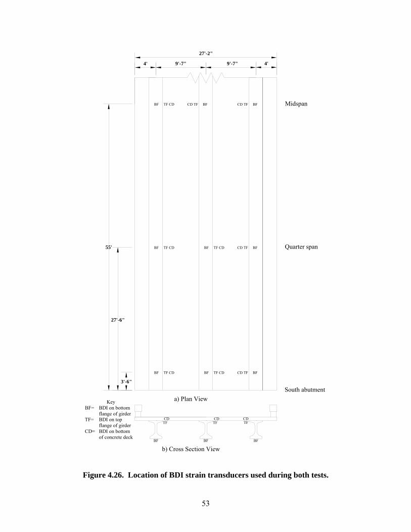
53
BF
TFCD
BF
TFCD
BF
TFCD
CD TF BFBF TF CD
3'-6"
27'-6"
55'
a) Plan View
b) Cross Section View
CD TF BF
BF TF CD BF TF CD CD TF BF
BF TF CD BF TF CD CD TF BF
27'-2"
4' 9'-7" 9'-7" 4'
KeyBF= BDI on bottom
flange of girderTF= BDI on top
flange of girderCD= BDI on bottom
of concrete deck
South abutment
Quarter span
Midspan
Figure 4.26. Location of BDI strain transducers used during both tests.

54
Table 4.5. Summary of test vehicle’s axle loads for Test 1.
Front Axle Weight (lbs) Rear Axle Weight (lbs) Total Weight (lbs)17,280 36,780 54,060
a) Side View - Loads
4'-7"17'-3"
7'-2" 6'-0"
b) Top View
c) Tandem truck used during Test 1
Figure 4.27. Test vehicle used in Test 1.

55
Table 4.6. Summary of test vehicle’s axle loads for Test 2.
Front Axle Weight (lbs) Rear Axle Weight (lbs) Total Weight (lbs)15,820 36,020 51,840
4'-5"15'-10"
7'-1" 6'-0"
a) Side View - Loads
b) Top View
c) Tandem truck used during Test 2
Figure 4.28. Test vehicle used in Test 2.
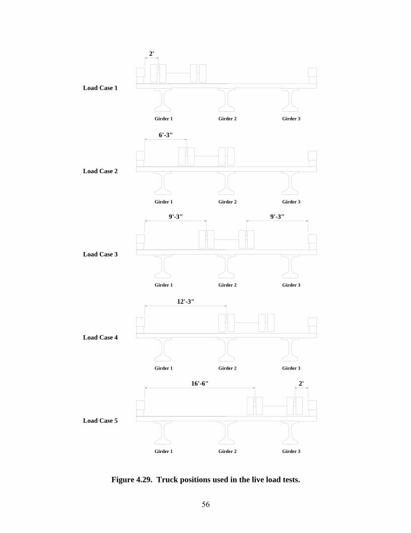
56
2'
6'-3"
9'-3"
12'-3"
16'-6"
Girder 1 Girder 2 Girder 3
Girder 1 Girder 2 Girder 3
Girder 1 Girder 2 Girder 3
Girder 1 Girder 2 Girder 3
Girder 1 Girder 2 Girder 3
Load Case 1
Load Case 2
Load Case 3
Load Case 4
Load Case 5
2'
9'-3"
Figure 4.29. Truck positions used in the live load tests.

57
CHAPTER 5: ANALYSIS METHODS
This chapter summarizes the analysis methods used both for assessment of the collected test data and the development of a UHPC shear design procedure. Computational procedures have been developed and are summarized herein for a UHPC beam member in both its uncracked and cracked conditions. For an uncracked section, standard mechanics of materials equations are used to compute stresses, strains, and deflections. When a cracked beam is analyzed at a section, strain compatibility and the MCFT are used. Also, a procedure for calculating deflection based on the sectional curvature along the entire member length is described.
5.1 Uncracked Beam Analysis
5.1.1 Sectional Analysis
In this section, calculation of stresses in the uncracked state is discussed. When the tensile principal stress reaches a value equivalent to the cracking strength of the material, the service level limit state is reached. This can be described mathematically as shown in equations 5.1 through 5.5. Note that transformed and composite section properties are used (which are described in more detail in Degen [16]).
x = c
cc
t
tt
I
cM
I
cM
I
ceP
A
P
longitudinal stress (ksi) (5.1)
Where: P = applied axial force (kips) A = gross cross-sectional area (in.2) e = eccentricity of axial force (in.) c = distance from centroid (in.) tc = distance from transformed centroid (in.)
cc = distance from composite centroid (in.)
I = moment of inertia (in.4) tI = transformed moment of inertia (in.4)
cI = composite moment of inertia (in.4)
tM = moment applied to transformed section (in.- kips)
cM = moment applied to composite section (in.- kips)
y = 0 vertical stress (ksi) (5.2)
xy = bI
QV
bI
QV
c
cc
t
tt
shear stress in the x-y plane (ksi) (5.3)
Where: tV = shear applied to transformed section (kips)
cV = shear applied to composite section (kips)
tQ = first moment about the neutral axis of the transformed section outside the shear

58
plane considered (in.3) cQ = first moment about the neutral axis of the transformed section outside the shear
plane considered for the composite section (in.3) b = width of section (in)
1p = 2
2
22 xyyxyx
principal tensile stress (ksi) (5.4)
2p = 2
2
22 xyyxyx
principal compressive stress (ksi) (5.5)
The compressive strength of UHPC was tested using a uniaxial compression test. The strength of each compression test specimen was determined using equation 5.6.
cf ` = A
Pmax maximum compressive strength of concrete (ksi) (5.6)
Where: maxP = maximum applied compressive force (kips)
A = gross cross-sectional area (in.2)
Flexural testing of prisms was completed to determine the tensile cracking strength of UHPC. The tensile cracking strength of the prisms was found using equation 5.7. There are some differences between flexural tension and direct tension; however, within this work they are considered interchangeable.
crf =
12
2323db
dLF
w
= 2db
LF
w
cracking tensile strength of concrete (ksi) (5.7)
Where: F = applied flexural cracking load (kips) L = span (in.)
wb = width of web (in.)
d = depth (in.) The service shear strength of UHPC can be determined theoretically using equation 5.4. The service shear strength is set as the shear force required to cause cracking. This occurs when the principal tensile stress is equated to the tensile cracking strength of the material. When this condition is true, the nominal service shear strength is given by equation 5.8. At this point when the concrete cracks, the crack orientation can be determined with equation 5.9 which is based upon Mohr’s stress circle. This value will be used later in the formulation of ultimate shear strength.

59
nV = ct VV nominal shear strength (kips) (5.8)
Where: tV = shear applied to transformed section (kips)
cV = shear applied to composite section (kips)
=
xt
cn
bI
QV
2
tan2
1 1 crack angle (degrees) (5.9)
Release stresses measured during release of the test beam and bridge beam can be verified using equation 5.10. This equation makes use of the mean stress method as described in reference [14] and is only valid in locations where the strand is fully developed.
f =
cicc
cicicxshx
EE
K
E
EE
K
ET
2
1
22
1
2
1
22
1
final stress due to prestress after losses (5.10) Where: x = longitudinal strain
sh = total shrinkage strain = 5.50×10-4
= thermal expansion coefficient = 6.55×10⁻⁶ per °F T = change in temperature (oF) cE = modulus of concrete = 7820 ksi
ciE = initial modulus of concrete = 5700 ksi
K = creep coefficient = 0.3 5.1.2 Deflection Analysis
Deflections are calculated in order to compare the experimental and analytical values to ensure understanding of the structural behavior of UHPC. The total deflection can be described as the superposition of the flexural and shear deflections as shown in equation 5.11. For an uncracked elastic section, these computations have been carried out using the unit load method. Any variety of methods would be acceptable.
= vm deflection due to moment and shear (in.) (5.11)
Where: m = deflection due to moment (in.)
v = deflection due to shear (in.)

60
5.2 Cracked Beam Analysis
In this section, methods for determining many different parameters of a cracked UHPC beam are discussed including the flexural strength, shear strength, stresses, strains, and curvature at a section. Note that the curvature computed at the sectional level will be used to make deflection calculations for the beam as a whole.
5.2.1 Sectional Analysis
For a cracked section, a non-linear flexural model was developed as part of this work. This model is sometimes referred to as the strain compatibility approach by ACI [9] and AASHTO [15] which is simply a sectional approach utilizing an iterative process. The procedure can be used to compute the ultimate moment capacity of a section or the deflection of a structural component. The analysis assumes that plane sections remain plane, that stress and strain can be related through constitutive material properties and that the shear stress is constant as shown in Fig 5.1.
Discretized Section Strain Stress ShearSection
Figure 5.1. General strain, stress, and shear within a section.
5.2.1.1 Flexural Analysis
For a purely flexural analysis, the strain compatibility approach is used but the influence of shear is ignored. Therefore, this procedure should be used in situations where shear deformations are negligible.
For this procedure, computer processing has been used to facilitate the iterative calculations which basically solve two equations with two unknowns. The two “unknowns” are the curvature and strain at one location along the section height using the assumption of linear strain profile. The specific location of the unknown strain could be set at any depth but has been arbitrarily chosen at the bottom flange. One of the “equations” results from force equilibrium (i.e., having a zero sum of forces in the horizontal direction at the sectional level). The other “equation” is satisfied by having the internal moment of the section equate to the external applied moment.

61
The external moment could be defined in one of two ways. First, the external moment could be the maximum possible applied moment or the moment capacity. In this case, Excel Solver was used to find the maximum value of the internal moment by iterating the strain and curvature and by satisfying force equilibrium. The second type of external moment is defined by the given loading conditions and is used for computing the deflection of a structural component. In this case, the curvature and strain are iterated to equate the internal and external moment and satisfy force equilibrium. Deflection can then be computed by integrating the curvature twice over the length of the beam. In the case of this research with a non-uniform beam having harped strands, the procedure must be repeated for many locations along the length. If the structural component being analyzed is uniform, a simpler approach could be utilized by defining one equation for the moment-curvature relationship.
In order to compute a moment capacity, the following example can be followed, which describes the computation of the capacity of the large-scale test beam at its midspan. First, the constitutive properties of the materials being used must be established. The idealized stress vs. strain diagrams used for the UHPC and the prestressing strands are shown in Figs. 5.2 and 5.3, respectively.
Next, the cross section of the beam is discretized into many rectangular segments of small heights across the full depth of the beam at each location as shown in Fig 5.1. With the assumption that plane sections remain plane, the strain profile must remain linear. Using an Excel spreadsheet, curvature and strain are iterated until a solution is found which satisfies the two previously described conditions. With this solution, the full strain profile can be determined as shown in Fig. 5.4. Combining the known strains with the constitutive properties of concrete, the stress profile of the concrete is created in Fig. 5.5.
-5
0
5
10
15
20
25
30
-0.03 -0.02 -0.01 0 0.01
Strain
Stre
ss (k
si)
Figure 5.2. UHPC compressive and tensile constitutive properties.

62
-300
-250
-200
-150
-100
-50
0
-0.05 -0.04 -0.03 -0.02 -0.01 0.00
Strain
Stre
ss (k
si)
Figure 5.3. Prestressing strand tensile constitutive properties.
Hei
ght (
in.)
0
6
12
18
24
30
36
42
-0.008 -0.006 -0.004 -0.002 0.000 0.002 0.004
Strain
Figure 5.4. UHPC strain profile at midspan of large-scale flexure test beam at nominal moment strength.

63
Hei
ght (
in.)
0
6
12
18
24
30
36
42
-4 0 4 8 12 16 20 24 28
Stress (ksi)
Figure 5.5. UHPC stress profile at midspan of large-scale flexure test beam at nominal moment strength.
The strains in the prestressing strands shown in Fig. 5.6 were determined by summing the prestressing strain with the strain induced by live loads. The stresses of the prestressing strands are shown in Fig. 5.7 and were determined by combining the strand strains with the constitutive strand properties.
Hei
ght (
in.)
0
6
12
18
24
30
36
42
-0.012 -0.010 -0.008 -0.006 -0.004 -0.002 0.000
Strain
Figure 5.6. Strand strain profile at midspan of large-scale flexure test beam at nominal moment strength.

64
Hei
ght (
in.)
0
6
12
18
24
30
36
42
-300 -250 -200 -150 -100 -50 0
Stress (ksi)
Figure 5.7. Strand stress profile at midspan of large-scale flexure test beam at nominal moment strength.
Next, a force resultant with its magnitude and position can be determined both in the compressive and tensile directions as shown in Fig. 5.8. The magnitudes of each must sum to zero for force equilibrium. Then the internal moment can be found by multiplying the distance between the two resultants by the magnitude of either one of the resultants. At this point, iteration takes place to maximize the internal moment.
3182 kips
42.00"33.54"
3182 kips
Figure 5.8. Force resultants at midspan of large-scale flexure test beam at nominal moment strength.

65
5.2.1.2 Flexure and Shear Analysis
For a combined flexure and shear analysis of a UHPC beam section, the purely flexural strain compatibility approach described in the previous section is combined with the shear analysis approach employing the MCFT [11]. Some parameters of the MCFT approach have been calibrated for use with UHPC using test data from the current research. Future research is needed to verify and add to the accuracy of the empirical parameters and the proposed approach in its entirety. The basic idea of the MCFT is to combine equilibrium, compatibility, and constitutive properties of the materials into an analysis based on average strains and stresses. The MCFT states some warnings of using this approach for a member without shear reinforcement. However, a UHPC section does have shear reinforcement in the form of fibers, not stirrups. Since the fibers in UHPC are oriented randomly, the contribution of the fibers is included in the tensile constitutive properties and not as a separate variable as is done in the case with shear stirrups in the MCFT. The presence of fibers also affects the analysis procedure recommended herein. The MCFT suggests analyzing the full stress-strain state at only one location within a section where the full stress-strain state is known because both the Mohr’s average stress and Mohr’s average strain circle are fully defined.
When employing the MCFT for use with UHPC, it is suggested that the full stress-strain state at many discrete locations along a section height should be analyzed. The main reasoning for this modification is because UHPC exhibits residual tensile stress across a crack in the longitudinal direction which is generally ignored with conventional concrete. When a plane section analysis is employed as described in the previous section, the stress profile can be predicted for conventional concrete by analyzing the full stress-strain state at only one location because the tensile strength of the concrete is essentially zero. In contrast, the stress profile is more accurately predicted for UHPC if many locations are used instead of just one. The directions of all the discussed stresses and strains are illustrated in Fig. 5.9 with stresses and strains occurring in the longitudinal, vertical, principal compressive, and principal tensile directions.
x x
yy p2
p2
p1
p1
Figure 5.9. Directions of stresses and strains in a general UHPC element.

66
The MCFT, as adopted in this research for combined flexure and shear analysis, is described as follows. A plane section analysis was used in conjunction with shear analysis. The curvature and the strain at the bottom of the section were first assumed for use with the plane section analysis as described in equations 5.12 and 5.13. These values were iterated until a solution was achieved and the strain was computed at every position along the section height as described by equation 5.14.
= guess curvature (1/in.) (5.12)
xb = guess longitudinal strain at bottom of section (5.13)
x = hxb longitudinal strain (5.14)
Where: h = distance above bottom of section (in.) Next, an estimate of the longitudinal stress was made. This estimate is based solely on the stress-strain constitutive relationship of UHPC described in section 2.1 and by equations 5.15 through 5.19.
If x 0 then,
xc =
2
``2`
c
x
c
xcf
longitudinal stress based on constitutive properties (ksi) (5.15)
If 0 x cr then,
xc = xcE longitudinal stress based on constitutive properties (ksi) (5.16)
If cr x min then,
xc = cr
cr
crxcr fff
maxmin
longitudinal stress based on constitutive properties (ksi) (5.17)
If min x max then,
xc = maxf longitudinal stress based on constitutive properties (ksi) (5.18)
If x max then,
xc = 0.672 ksi xln + 2.362 ksi 0 ksi
longitudinal stress based on constitutive properties (ksi) (5.19)
Where: crf = cracking tensile strength of concrete = -1.1 ksi
maxf = maximum tensile strength of concrete = -1.7 ksi
cr = cracking tensile strain of concrete = -0.000141
max = maximum magnitude of strain corresponding to maxf = -0.0024
min = minimum magnitude of strain corresponding to maxf = -0.0014

67
However, due to a bilinear state of stress within a structural element, the constitutive property relationship, which is based on uniaxial testing, is not fully valid. A material becomes weaker or “softer” in one direction when tension is applied in a perpendicular direction. The MCFT has developed equations relating the stress in the principal compressive direction to the strain in the principal tensile direction. In order to ease computation the “softening” relationship will be assumed to be applicable between the longitudinal stress and the vertical strain. In addition, the same softening affect will be assumed to take place for longitudinal tensile stresses due to vertical tensile strains. This relationship is not discussed by the MCFT because residual tensile stresses in the longitudinal direction are negligible in conventional concrete but not for UHPC. The following procedure, up to equation 5.26, is performed in order to find the “softened” longitudinal stress.
Shear contributes to the “softening” of concrete. The MCFT assumes a shear stress distribution as being constant along the lever arm height “jd” and zero at other locations as shown in Fig. 5.1. The shear stress magnitude is described by equation 5.20. A shear stress distribution is assumed instead of being calculated because of the complexity of this approach. A dual-section analysis could be completed in order to more correctly calculate the shear stress. In this approach two sections within a beam which are quite close together are analyzed. The difference in the longitudinal stresses between the two sections requires shear stress to satisfy equilibrium. As has been discussed, shear contributes to the softening of concrete, thus altering the longitudinal stresses. This interdependency between the longitudinal and shear stresses makes the solution technique challenging.
xy = djb
V
w shear stress in the x-y plane (ksi) (5.20)
Where: V = applied shear (kips) wb = width of web (in.)
j = lever arm percentage of depth d = depth (in.)
The lever arm height can be determined by a secondary iteration. An initial assumption is provided by the MCFT which states that the lever arm (i.e., j*d) need not be taken any smaller than 80% of the section height. Once the full computation of section 5.2.1 has been carried out, the distance between the compressive force resultant and the tensile force resultant can be compared to the initial assumption and a more refined value can be found.
Next, the shear strain can be determined using the shear stress-strain relationship developed during this research as shown subsequently in Fig. 6.22. The relationship is linear following the shear modulus until a stress of 2.3 ksi is reached. Then a parabolic relationship is used to a maximum stress of 3.5 ksi and strain of 0.01 as described in equations 5.21 and 5.22.

68
If xy cr then,
xy = G
xy shear strain in the x-y plane (ksi) (5.21)
Where: G = shear modulus (ksi) = 3258 ksi If xy cr then,
xy =
cr
crxy G
max
2
maxmax
max shear strain in the x-y plane (5.22)
Where: max = maximum shear strain = 0.01
cr = cracking shear stress = 2.3 ksi
max = maximum shear stress = 3.5 ksi
The MCFT theory has developed equation 5.23 to relate the “softening” effect on stress due to strain in the orthogonal direction. The left hand side of the equation that is multiplied by σxc can be thought of as a softening factor. This term is always less than one because the concrete becomes weaker with an applied orthogonal strain. The MCFT uses a first softening coefficient of ξ1 = 0.8, in which case if the vertical strain were zero, the entire softening term would be greater than one. Therefore, the MCFT states that the entire term cannot be greater than one. However, within the procedure used herein, it is mathematically difficult to use this inequality statement. Therefore, the first softening coefficient has been set equal to one, so the entire softening term will never be greater than one. Based upon the experimental results discussed in Chapter 6, the second softening coefficient has been estimated as ξ2 = 3. The MCFT uses a value of 0.34 for normal concrete. This large discrepancy is due to the use of a different material with a larger maximum strain, a different solution procedure taking into account every location along the height of the member instead of only one location, and that the longitudinal and vertical directions are being related instead of the two principal directions.
All the basic information is now available to determine the “softened” longitudinal stress. There are six unknown values needed in order to fully define the stress-strain state at any one location of the beam. This is because in order to fully define Mohr’s circle of average stresses, three values must be known. Three values must also be known to define Mohr’s circle of average strains. As discussed, the shear stress, shear strain, and longitudinal strain are known. In addition, the vertical stress can be assumed to be zero. One assumption made by the MCFT and upheld herein is that the angle of principal compressive stress is equal to the angle of the principal compressive strain. This eliminates the need for one known value.
Now there are three unknowns, namely the longitudinal stress, principal compressive stress angle, and vertical strain. Equation 5.23 has been developed by the MCFT to define the longitudinal stress. Using Mohr’s circle of average stresses and strains shown in Fig. 5.10 and 5.11, equations 5.24 and 5.25 can be derived describing the principal compressive stress angle and the vertical strain.

69
xy
x
y
normalstress
p2p1
2
shearstress
Figure 5.10. Mohr’s circle of average concrete stresses in a general UHPC element [5].
x
normalstrain
2
shearstrain
p2 p1
y
2
xy2
Figure 5.11. Mohr’s circle of average concrete strains in a general UHPC element [5].

70
x = xc
c
y
`
1
21
longitudinal stress (ksi) (5.23)
Where: 1 = first softening coefficient = 1
2 = second softening coefficient = 3
c̀ = strain associated with f`c
y = vertical strain
=
x
xy
2
tan2
1 1 principal compressive stress angle (degrees) (5.24)
y =
2tanxy
x vertical strain (5.25)
In order to develop a solution, a third order system of equations must be solved (equations 5.23 through 5.25). First, of equation 5.24 can be substituted into equation 5.25 resulting in equation 5.26. Then substituting y from equation 5.26 into equation 5.23 results in equation
5.27. If equation 5.27 is rearranged, equation 5.28 is derived.
y = xy
xxyx
2 vertical strain (5.26)
x =
xy
xxyxc
xcc
2`
`
21
longitudinal stress (ksi) (5.27)
xccxxcxxxy
xy
21
2 `2
= 0 ksi quadratic equation (5.28)
The quadratic equation described by equations 5.29 through 5.33 is utilized as a solution technique for equation 5.28 resulting in the derivation of the “softened” longitudinal stress described by equation 5.34.
qxqxq CBA 2 = 0 ksi quadratic equation (5.29)
If xc 0 ksi then,
qA = xy
xy
22 second order quadratic equation coefficient (in.2/kip) (5.30)
If xc 0 ksi then,

71
qA = xy
xy
22 second order quadratic equation coefficient (in.2/kip) (5.31)
qB = xc 21 ` first order quadratic equation coefficient (5.32)
qC = xcc ` constant quadratic equation coefficient (ksi) (5.33)
x = q
qqqq
A
CABB
2
42
longitudinal stress (ksi) (5.34)
This process will cause a mathematically erroneous answer for portions of the section with zero shear stress due to division by zero. Therefore, it has been assumed that the softening coefficient is constant across the section height set at the value computed at the beginning of the moment arm region.
Once the longitudinal stress is known, the plane section nonlinear flexural model described in section 5.2.1.1 is used. In that case, strain and curvature were solved based on moment and axial load. Now, in addition to those quantities, if the shear force is given, the shear stress distribution can also be determined which, in turn, impacts the other quantities. Utilizing a computer algorithm and/or an Excel spreadsheet with solver, the iterative calculations can be completed. The solution process is similar to solving three equations with three unknowns. Excel solver has a feature which allows the maximum value of shear force to be determined. Therefore, not only can this procedure be used with a given shear force, but it can also be used to determine shear strength.
To illustrate an example of the previous description several figures are shown. Figures 5.12 through 5.16 show the unsoftened longitudinal stress, vertical strain, principal compressive stress angle, softening coefficient, and the softened longitudinal stress analyzed at load application point L4 (see Fig. 4.12) for the flexure-shear beam test at a total load of 600 kips.
In order to determine the maximum value of shear, different failure modes should be analyzed. The modes that have been identified for this research are flexural tension failure, flexural compression failure, flexural tension failure of strands, compression failure of a web strut caused by shear, and tension failure of the web caused by shear. When flexural tension failure of the UHPC flange occurs, the longitudinal tension strain within the flange becomes large enough for the concrete to lose strength as described by its constitutive properties in section 2.1. The same is true for compression failure of the UHPC flange but large compression strains are developed instead of tension. Flexural tension failure of the strands occurs when the tensile strain in the strands exceeds the strain capacity. Shear compression failure of the web strut occurs when the principal compressive stress equates to the compressive strength of UHPC which can be determined with cylinder testing and a “softening” analysis. Shear tension failure of the web occurs when the principal tensile strain of UHPC becomes too large. This value can be obtained by multiplying the crack spacing by the maximum inclined crack width in the UHPC beam. Both of these parameters will need further research to fully define.

72
0
6
12
18
24
30
36
42
-5 0 5 10 15 20 25
Stress (ksi)
Hei
ght (
in.)
Figure 5.12. Unsoftened longitudinal stress of large-scale flexure-shear test beam at load application point L4 while undergoing a total load of 600 kips.
0
6
12
18
24
30
36
42
-3.0E-03 -2.5E-03 -2.0E-03 -1.5E-03 -1.0E-03 -5.0E-04 0.0E+00
Vertical Strain
Hei
ght (
in.)
Figure 5.13. Vertical strain of large-scale flexure-shear test beam at load application point L4 while undergoing a total load of 600 kips.

73
0
6
12
18
24
30
36
42
0 10 20 30 40 50
Principal Compressive Stress Angle (degrees)
Hei
ght (
in.)
Figure 5.14. Principal compressive stress angle of large-scale flexure-shear test beam at load application point L4 while undergoing a total load of 600 kips.
0
6
12
18
24
30
36
42
0.0 0.2 0.4 0.6 0.8 1.0
Softening Coefficient
Hei
ght (
in.)
Figure 5.15. Softening coefficient of large-scale flexure-shear test beam at load application point L4 while undergoing a total load of 600 kips.

74
0
6
12
18
24
30
36
42
-2 0 2 4 6 8 10 12 14
Stress (ksi)
Hei
ght (
in.)
Figure 5.16. Softened longitudinal stress of large-scale flexure-shear test beam at load application point L4 while undergoing a total load of 600 kips.
5.2.2 Deflection Analysis
The following describes a procedure for determining beam deflections in the elastic or post-elastic range after cracking. The beam is first discretized into many small portions along its length. Given a particular loading condition, the external moments corresponding to each location along the beam length can be found and set equal to the internal moments at each location. When this process is completed, the curvature at the discrete locations along the length of the beam can be determined. Next, two integrations of the curvature over the length of the beam are performed. It is not practical to express the curvature in closed form for a cracked beam because a very complicated equation would be required. Therefore, numerical integration is used. In the case of this research, the trapezoidal rule has been used although any numerical integration technique is acceptable. By integrating the curvature over the beam length, the slope can be found. However, an initial value for the slope must be determined in an iterative process. Integrating the slope numerically will determine the value of the deflection as shown in equation 5.35. The initial deflection at both ends of the beam must be equated to the boundary conditions which in most cases is zero. The solution is found by iteratively solving for the initial slope of the beam which can be done using Excel Solver as was done in this research.
= dxdxx x
0 0
deflection due to moment and shear (in.) (5.35)
Where: = curvature (1/in.) x = position along length of beam (in.)

75
Deflections computed using this procedure have been verified by comparing them to experimental deflections obtained during the FHWA structural testing described in section 2.4. Using the procedure of section 5.2.1.1, Fig. 5.17 shows that for the FHWA Flexure Test the experimental and analytical deflections correlate fairly well. Also, FHWA Shear Test #2 was analyzed using the procedure of section 5.2.1.2. The results did not match well. It should be noted that Chuang and Ulm [12] completed analysis on this test which closely match the analysis done in this work. The experimental deflection is shown in Fig. 5.18 to be approximately a constant 1.4 times larger than the analytical deflection. Possible reasons for this discrepancy are previous damage to the beam, underestimation of shear deformation, errors in the experimental data, or strand slip. Some previous damage did occur in the beam because the broken portion of the FHWA Flexure Test beam was used for the FHWA Shear Test #2. Analytically, shear deformation accounted for approximately 9% of the total deflection of the FHWA Shear Test #2 within the linear range.
5.2.3 Strut and Tie Analysis
Strut and tie analysis has been carried out according to section 2.3 and the provisions of ACI [9]. The computations show that the concrete is sufficiently strong in compression in order not to fail the struts when a strut factor of 0.85 is used. Therefore, the applied load is iterated until the tension in the tie reaches its ultimate capacity or until the angle between the strut and tie reaches 25 degrees as dictated by the strut and tie method. Degen [16] provides an example of the strut and tie method for the small-scale beams conducted as part of this research.
0
50
100
150
200
0 5 10 15 20
Deflection (in.)
Tot
al L
oad
(kip
s)
Experimental
Analytical
Figure 5.17. Deflection of FHWA Flexure Test beam at midspan.

76
0
100
200
300
400
500
600
700
800
0.00 0.25 0.50 0.75 1.00 1.25 1.50 1.75 2.00
Deflection (in.)
Tot
al L
oad
(kip
s)
Experimental
Analytical
Figure 5.18. Deflection of FHWA Shear Test #2 beam at the load application point.

77
CHAPTER 6: EXPERIMENTAL AND ANALYTICAL RESULTS
This chapter describes the experimental and analytical results for this research. Where appropriate, results include qualitative observations, quantitative data and interpretations of the data.
6.1 Material Testing
6.1.1 Uniaxial Compression Testing
Uniaxial compression strengths were determined using the previously described procedure in section 5.1.1. The average and standard deviation strength values are summarized in Table 6.1 for three different groups of samples; those cured at 194°F in a controlled chamber, those cured with the product, and those cured at room temperature. As a whole, the samples had slightly lower strength than the anticipated strength of 28 ksi (section 2.1). It is apparent that curing the samples in a controlled chamber at 194°F resulted in the highest compressive strength, while curing with the product was slightly lower but with greater consistency. Curing at room temperature resulted in the lowest strengths.
Table 6.1. Uniaxial compressive strength of UHPC cubes.
Curing Method Average (ksi) Standard Deviation (ksi)194°F 25.12 4.32
With Product 24.56 2.91Room Temperature 21.5 3.98
6.1.2 Prism Flexural Testing
In general, flexural testing of the prism specimens caused them to first crack in the central constant moment region as expected. After cracking, the prisms held additional load until failing in that same region. For this work, the load at which the load vs. table displacement became non-linear was defined as the flexural cracking load as is illustrated in Fig. 6.1 at a load of about 0.9 kips. The cracking tensile stress can be calculated using equation 5.7, which is not valid after cracking. The resulting flexural tensile cracking strength statistics are summarized in Table 6.2 for the three different curing conditions. Curing at 194°F resulted in the highest strengths, while curing at room temperature resulted in the lowest strengths. In general, the flexural tensile cracking strength results relate well to previously published test results [1], [2], [3], and [4].

78
0
0.5
1
1.5
2
2.5
3
3.5
4
4.5
0 0.02 0.04 0.06 0.08 0.1 0.12 0.14
Table Displacement (in.)
Loa
d (k
ips)
Figure 6.1. Load vs. table displacement during a typical prism flexure test.
Table 6.2. Flexural cracking tensile strength of UHPC prisms.
Curing Method Average (ksi) Standard Deviation (ksi)194°F -1.16 0.21
With Product -1.04 0.12Room Temperature -0.93 0.12
6.2 Large-Scale Laboratory Testing
6.2.1 Flexural Testing
6.2.1.1 Test Observations
During testing, the beam was inspected for cracks three times. The first inspection occurred at a total load level of approximately 237.4 kips and revealed one very small hairline crack near the beam midspan which was subsequently verified to be a crack during the second sequence of loading. The second inspection took place at a total load level of approximately 256 kips during the second sequence of loading when 13 hairline cracks spaced at about 6 in. were discovered on the bottom flange of the beam within the constant moment region. The third and final inspection took place at the end of the second sequence of loading at a total load level of approximately 265 kips. At this point, the previously identified cracks had extended. Also, one new crack was found nearly at the midspan of the beam. This flexural crack extended up to the web region of the beam on the north side (higher than any of the other cracks) and extended about 3 in. up from the bottom flange on the south side (lower than any of the other cracks). All 14 cracks ran transversely across the entire bottom flange of the beam. The cracks on the north face ended within the tapered portion of the bottom flange, while the cracks on the south side ended near the beginning of the tapered portion of the bottom flange. Generally, the cracks could be classified

79
as “hairline”. The cracks were marked with typical examples shown in a close up view on the bottom flange of the north face of the beam in Fig. 6.2. On the east end of the beam, the concrete around one strand had several cracks extending in the radial direction around the strand perimeter. On the west end of the beam, horizontal and vertical cracks extended to both the side and bottom of the beam at each of the two bottom corner strands.
Figure 6.2. Flexural cracks on north bottom flange at midspan at peak load of large-scale flexure test.
6.2.1.2 Test Results
The primary purpose of the flexure test was to provide reassurance to the design engineer that the beam had sufficient capacity for implementation in the first United States UHPC bridge in Wapello County, Iowa. This was achieved by reaching a load level above the expected service loads before cracking had occurred. The service level is determined by a simple summation of external moments required to be resisted by the bridge beam, which included moment from the bridge deck, future overlay, barriers, and the live load as required by code. Using the effective width of the bridge deck according to AASHTO [15], the bridge beams have a larger section than the test beam and therefore can resist even more moment. As can be seen in Fig. 6.3, the total load when non-linearity occurs at cracking was 237.4 kips which corresponds to a moment of 3,730 ft-k, without including the beam self-weight. Using this information and the additional effective width of the slab, a service moment capacity of the bridge beam can be determined which should be larger than the applied service moment as shown in Table 6.3. The same type of process was carried out for the ultimate limit state. However, test data for this beam did not reach this level, and therefore, the quantities shown in Table 6.3 are based off of analysis rather than testing.

80
0
50
100
150
200
250
300
-750 -500 -250 0 250 500 750 1000 1250
Microstrain
Tot
al L
oad
(kip
s)
Gage #11
Gage #12
Figure 6.3. Strain at midspan during large-scale flexure test.
Table 6.3. Comparison of large-scale flexure test capacities to applied bridge moments.
Service Level 3,730 4,760 4,624Ultimate Level N/A 7,620 7,350
Limit State
Experimental Moment Capacity of Test Beam (ft-kips)
Analytical Moment Capacity of Bridge Beam (ft-kips)
Applied Moment on Bridge Beam (ft-kips)
In addition, the flexure test was useful for estimating the amount of prestressing in the test beam. By using the applied moment at which cracking occurred, the prestressing force was estimated to be 1517 kips (27.2% loss) experimentally using a simple linear stress analysis. The amount of prestressing determined experimentally was also compared with traditional calculations made during initial design. The losses that were accounted for are the initial relaxation, elastic shortening, shrinkage, creep, and secondary relaxation. These loss calculations are described by AASHTO [15] and are documented in Degen [16] using the material properties presented previously. The calculated analytical prestressing force after losses is 1450 kips (30.4% loss) which correlates fairly well with the experimental results.
Several instruments recorded data during the test to ensure that the beam was behaving as expected. The deflection at several locations could be accurately calculated within the linear range by using the unit load method. Figure 6.4 shows the midspan experimental and analytical deflection. As well, the stresses within the beam could be predicted accurately. For instance, in Fig. 6.5 the stresses at midspan under a total load of 237 kips are shown to be accurate and uphold the assumption that plane sections remain plane. In addition, three strands were monitored for slip. One gage indicated a rapid increase in slip to 0.005 in. at the maximum load as shown in Fig. 6.6.

81
0
100
200
300
400
500
600
0 2 4 6 8 10 12
Deflection (in.)
Tot
al L
oad
(kip
s)
Experimental
Analytical
Figure 6.4. Deflection at midspan during large-scale flexure test.
-7
0
7
14
21
28
35
42
-8 -6 -4 -2 0 2 4 6 8 10
Stress (ksi)
Hei
ght (
in.)
Experimental
Analytical
Figure 6.5. Longitudinal live load stresses at cracking of large-scale flexure test beam.

82
0
50
100
150
200
250
300
-0.001 0.000 0.001 0.002 0.003 0.004 0.005 0.006
Slip (in.)
Tot
al L
oad
(kip
s)
Figure 6.6. Strand slip at gage S1 during large-scale flexure test.
6.2.2 Shear Testing
6.2.2.1 Test Observations
Throughout the test, the beam was periodically inspected and cracks were marked. At a total load of 369.8 kips, shear cracking first occurred in the end region of the beam. As shown in Fig. 6.7, crack #1 extended at approximately a 25 degree angle from the top of the web about 1 ft from the first applied load to the bottom of the web and approximately 2 ft away from the abutment. Using equation 5.9, the crack angle can be computed as 25.3 degrees at the bottom of the web and 23.3 degrees at the top of the web. As loading resumed, several more inclined shear cracks developed. At a total load of 397.6 kips, flexural cracks occurred under the east-most applied load, extending about 2 in. up from the bottom flange. This region was not cracked in the previous flexure test. At this time it was also observed that some, but not all, of the transverse cracks caused by the flexural test on May 11th had extended a short distance. Also, new longitudinal cracks were observed at the top of the bottom flange near the bottom of the web, possibly due to bursting of the concrete around the bottom flange strands.
When the beam failed at a total load of 594.0 kips, crack #2 (not crack #1) was the most prominent within the failure region as shown in Fig. 6.7. After failure and additional subsequent loading, crack #2 was about 1 in. wide. Crack #2 extended from the top of the web near the second applied load (L2 in Fig. 4.7) to the bottom of the web at the location of a lifting loop. This lifting loop is assumed to have shifted the failure critical region of the beam and to have added slightly to the ultimate shear strength at this location. Additional unexpected cracking was found at the end of the beam. The beam was sitting on two independent neoprene pads that separated horizontally during the test. This may have caused half of the beam to move with each pad and created a vertical cracked plane from the bottom of the beam up to the harped strands as
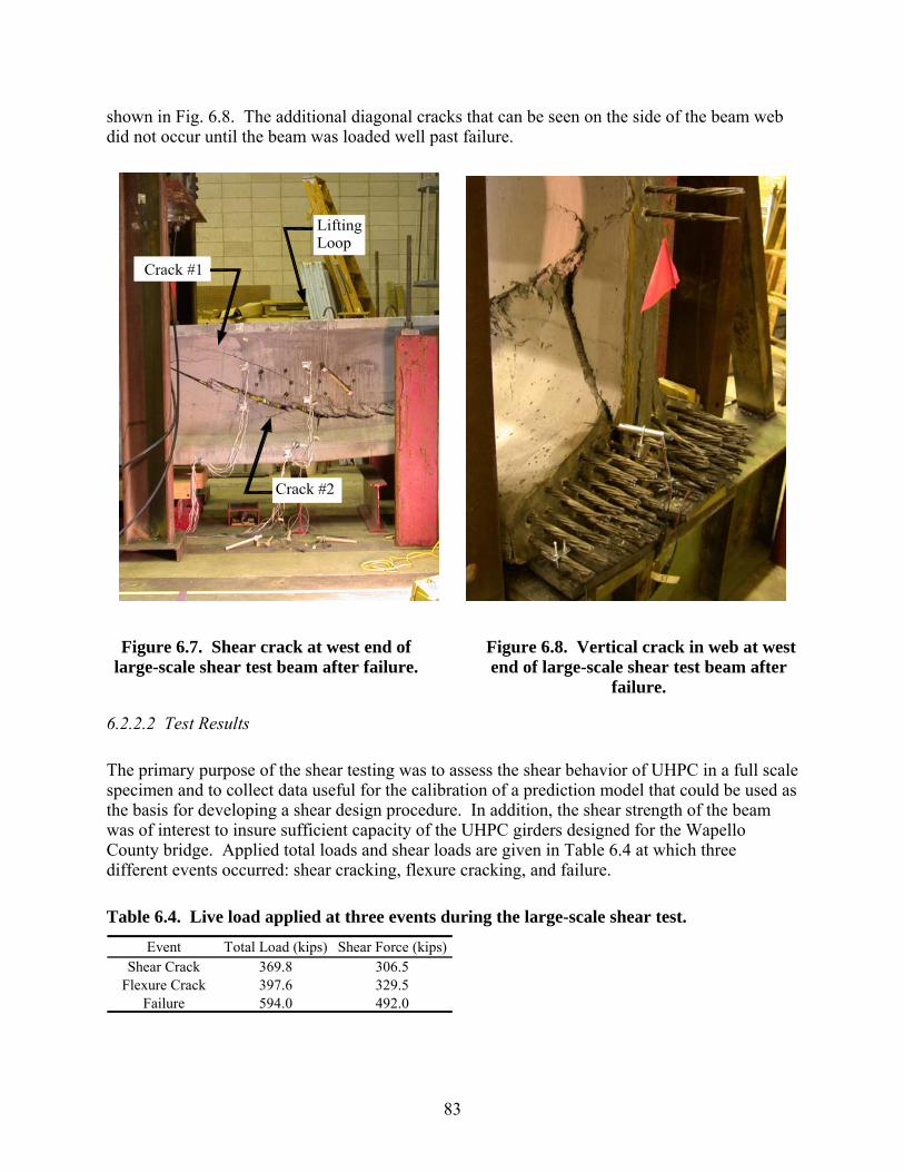
83
shown in Fig. 6.8. The additional diagonal cracks that can be seen on the side of the beam web did not occur until the beam was loaded well past failure.
Figure 6.7. Shear crack at west end of large-scale shear test beam after failure.
Figure 6.8. Vertical crack in web at west end of large-scale shear test beam after
failure.
6.2.2.2 Test Results
The primary purpose of the shear testing was to assess the shear behavior of UHPC in a full scale specimen and to collect data useful for the calibration of a prediction model that could be used as the basis for developing a shear design procedure. In addition, the shear strength of the beam was of interest to insure sufficient capacity of the UHPC girders designed for the Wapello County bridge. Applied total loads and shear loads are given in Table 6.4 at which three different events occurred: shear cracking, flexure cracking, and failure.
Table 6.4. Live load applied at three events during the large-scale shear test.
Event Total Load (kips) Shear Force (kips)Shear Crack 369.8 306.5
Flexure Crack 397.6 329.5Failure 594.0 492.0

84
The service and ultimate capacities of the test beams were determined as shown in Table 6.5 by including dead load and prestressing with the tested cracking and failure shear forces. The bridge beams were assumed to have the same capacities. As shown, the shear capacities were greater than the applied shear forces, making an acceptable design.
Table 6.5. Comparison of large-scale shear test capacities to applied bridge shears.
Service Level 312 312 210Ultimate Level 497 497 301
Analytical Shear Capacity of Bridge Beam (kips)
Applied Shear on Bridge Beam (kips)
Limit State
Experimental Shear Capacity of Test Beam (kips)
The load at which shear cracking occurred can be determined as the point when measured strains are no longer linear as shown in Fig. 6.9. Gage “a” refers to horizontal strain, “b” to strain at a positive 45 degree angle and “c” to strain at a negative 45 degree angle. The load at flexural cracking was determined using the point of non-linearity in Fig. 6.10. Both the shear cracking and flexural cracking load levels corresponded to slight discontinuities in the deflection data, thus verifying the loads at cracking. The load at failure was simply determined as the maximum load applied during testing as shown in Fig. 6.11.
Figure 6.11 shows the analytical deflection calculated using the procedure described in section 5.2.1.2. The softening coefficients mentioned in Chapter 5 were back-calculated as was previously discussed to best match the analytical and experimental deflections. Shear deformation accounts for 4% of the deflection in this instance. This procedure can be compared to that described in section 5.2.1.1, where the impact of shear on deflection is ignored resulting in the analysis shown in Fig. 6.12.
0
100
200
300
400
500
600
-400 -200 0 200 400 600
Microstrain
Tot
al L
oad
(kip
s)
Gage #2a
Gage #2b
Gage #2c
Figure 6.9. Strain at gage #2 during large-scale shear test.

85
0
100
200
300
400
500
600
700
-800 -700 -600 -500 -400 -300 -200 -100 0
Microstrain
Tot
al L
oad
(kip
s)
Figure 6.10. Strain at gage #10 during large-scale shear test.
0
100
200
300
400
500
600
700
0 1 2 3 4
Deflection (in.)
Tot
al L
oad
(kip
s)
Experimental
Analytical
Figure 6.11. Deflection including shear analysis at gage D3 during large-scale shear test.

86
0
100
200
300
400
500
600
700
0 1 2 3 4
Deflection (in.)
Tot
al L
oad
(kip
s)
Experimental
Analytical
Figure 6.12. Deflection excluding shear analysis at gage D3 during large-scale shear test.
Analytical beam capacities were computed for comparison to experimental values. Following the procedure described in section 5.1.1, the service shear and flexural strengths were determined. The service shear strength was estimated as 303 kips while the corresponding measured value was 312 kips, showing that cracking could be accurately predicted. The flexural cracking was also accurately predicted at a total load of 405 kips as compared to the measured load of 397.6 kips. For the ultimate limit state, the failure mode was observed to be shear tensile failure of the UHPC web. At the experimental failure load, the principal tensile strain was determined analytically to be 0.00125. Multiplying the principal tensile strain at failure by the crack spacing results in a crack width at failure. Further research should be conducted to accurately predict the crack spacing of UHPC under shear and to determine a crack width that will induce failure. During this research microcracks were observed at approximately 2 in. of crack spacing. However, the crack spacing of localized cracks should be used. This value was not available during testing because essentially one primary localized crack formed. A secondary crack was observed but it is thought to have occurred due to the shifting of the primary crack which crossed a vertical prestressing strands used as a lifting loop.
Throughout the shear test, strand slip was measured on three different strands. Slip did not occur on two of the strands. Some strand slip did occur in one of the three strands that were investigated as shown in Fig. 6.13. Other strands may have slipped as well.
The live load principal stresses in the beam could be calculated and compared to experimental data up to the point of shear cracking as shown in Fig. 6.14. After shear cracking, the experimental strain data are difficult to interpret due to discontinuities caused by shear cracking. All of the gages showed fairly good correlation between the analytical and experimental values showing that the elastic behavior of the beam was satisfactorily captured. There is some discrepancy between the experimental and analytical values, which could be caused by misalignment of the strain gage rosettes or by arching action in the end of the beam. The total

87
principal stresses shown in Fig. 6.15 included prestressing, dead load, and live load so that the results are no longer linear as with live load alone. The total principal stresses began to show discontinuos behavior after exceeding the shear cracking load of 369.8 kips. Generally, all the gages showed total principal tensile stress at the cracking stress of approximately -1.1 ksi as expected.
0.00
0.10
0.20
0.30
0.40
0 1 2 3 4 5
Deflection at Gage #3 (in.)
Slip
(in.
)
Figure 6.13. Strand slip at gage S3 during large-scale shear test.
0
50
100
150
200
250
300
350
400
-3 -2 -1 0 1 2 3
Stress (ksi)
Tot
al L
oad
(kip
s)
Experimental
Analytical
Figure 6.14. Live load principal stresses at gage #2 during large-scale shear test.

88
0
50
100
150
200
250
300
350
400
-2 -1 0 1 2 3 4 5
Stress (ksi)
Tot
al L
oad
(kip
s)
Experimental
Analytical
Figure 6.15. Total load principal stresses at gage #2 during large-scale shear test.
6.2.3 Flexure-Shear Testing
6.2.3.1 Test Observations
Throughout the test, the beam was periodically inspected and cracks were marked. The first cracks to be observed were flexural cracks occurring at a total load of 366.9 kip. These were vertical cracks located near load application point L2 identified in Fig. 4.12. No shear cracks were found in this region throughout testing. At this point and thereafter, the beam could be heard to be cracking repeatedly.
As loading continued, shear cracking occurred at a total load of 481.8 kips. Diagonal shear cracks were found in the end region of the beam between the support and load point L4 in Fig. 4.12 as shown in Fig. 6.16. After additional loading, flexure cracks began to occur in this region. The shear cracks were seen to bend from the diagonal direction within the web toward the vertical direction within the bottom flange. During additional loading, longitudinal cracks near the original midspan of the flexure test were observed. Furthermore, a vertical-longitudinal splitting crack could be seen at the east end of the beam going through the center of the beam where no strands were present. This crack was much smaller than a similar crack which occurred at the opposite end of the beam during the shear test shown in Fig. 6.8. Eventually, little additional load was being applied to the beam, and the beam continued to deflect to a maximum of 8.5 in. at the easternmost load point when testing was ended at a total load of 658.1 kips.

89
Figure 6.16. Flexure and shear cracking near gage R1 at a total load of 482 kips during the large-scale flexure-shear test.
6.2.3.2 Test Results
The purpose of the flexure-shear test was to determine the behavior of UHPC under combined flexure and shear loading. Loads are given in Table 6.6, at which three different events occurred: flexure cracking, shear cracking, and the maximum applied load which is determined to be near the failure load. The total load at flexure cracking is seen in Fig. 6.17 when the strain becomes non-linear. The total load due to shear cracking was determined at the point when strains have a discontinuity as shown in Fig. 6.18. The maximum applied load can be seen in Fig. 6.19.
Table 6.6. Live load applied at three events during the large-scale flexure-shear test.
Event Total Load (kips) Shear Force (kips)Flexure Crack 366.9 226.1Shear Crack 481.8 296.1Maximum 658.1 404.2
The large-scale flexure-shear test resulted in nearly maximizing the load that could safely be applied. No actual failure took place which can normally be described by a drop in applied load. However, it appears by the flattening of the load vs. deflection curve that a load near failure was achieved although additional deflection would have occurred. The beam was analyzed using the procedure outlined in section 5.2.1.2. The maximum total load applied during the test was 658 kips with an analytically predicted failure load of 649 kips which corresponds to 404 kips and

90
399 kips of shear force, respectively. In addition, the deflection values correlate well as shown in Fig. 6.19 where 4% of the deflection is due to shear deformation.
0
100
200
300
400
500
600
700
-5000 -4000 -3000 -2000 -1000 0
Microstrain
Tot
al L
oad
(kip
s)
Figure 6.17. Strain at gage F5 during large-scale flexure-shear test.
0
100
200
300
400
500
600
700
-400 -200 0 200 400
Microstrain
Tot
al L
oad
(kip
s)
Gage #17a
Gage #17b
Gage #17c
Figure 6.18. Strain at gage #17 during large-scale flexure-shear test.
The live load principal stresses were measured within the web with a strain rosette and are shown in Fig. 6.20. The analytical and experimental results generally correlate. In general, the gages show that an approximate total principal stress of -1.1 ksi is reached at cracking within the failure region as shown in Fig. 6.21 at a total load of 481.8 kips. This agrees with the tested cracking strength reported for the material properties in section 2.2. Strand slip was measured at

91
three strands at the end of the beam closest to the applied loads. No significant slip to these three strands was observed throughout the test.
0
100
200
300
400
500
600
700
0 2 4 6 8 10
Deflection (in.)
Tot
al L
oad
(kip
s)
Experimental
Analytical
Figure 6.19. Deflection at gage D5 during large-scale flexure-shear test.
0
100
200
300
400
500
-3 -2 -1 0 1 2 3
Stress (ksi)
Tot
al L
oad
(kip
s)
Experimental
Analytical
Figure 6.20. Live load principal stresses at gage #17 during large-scale flexure-shear test.
Using data from the shear test and the flexure-shear test, an idealized shear stress-strain relationship can be formulated. The idealized relationship is expressed mathematically in Chapter 5 as being linear until a stress of 2.3 ksi is reached, at which point the stress-strain relationship follows a parabolic relationship. Figure 6.22 shows data for two different tests, with the idealized relationship representing roughly an average of the two experimental data sets. This data was collected with the large wooden dowel strain gage rosettes shown in Figs. 4.11 and

92
4.16. These gages helped to overcome the effects of localized cracking because their gage lengths were 10 in. which is much longer than a typical strain rosette. However, the gages did fall off during testing when cracks were formed at the locations where the gages were glued to the beam. Drilling such gages into the beam would probably result in better data.
0
100
200
300
400
500
-2 -1 0 1 2 3 4
Stress (ksi)
Tot
al L
oad
(kip
s)Experimental
Analytical
Figure 6.21. Total load principal stresses at gage #17 during large-scale flexure-shear test.
Stre
ss (k
si)
0
0.5
1
1.5
2
2.5
3
3.5
0 0.002 0.004 0.006 0.008 0.01
Strain
Idealized
Gage R2 ShearGage R2 Flexure-Shear
Figure 6.22. Shear constitutive properties of UHPC.

93
6.3 Small-Scale Laboratory Testing
6.3.1 Test Observations
During testing of the small-scale beams, observations were recorded throughout testing without pauses in the loading. In each of the beams, cracking occurred either due to flexure or shear at a load level ranging from 47 kips to 82 kips as shown in Table 6.7. As loading continued to a peak load ranging from 116 kips to 164 kips as shown in Table 6.7, strand slip occurred in each of the beams and localized flexure or shear cracks formed.
Table 6.7. Live load and shear force applied at cracking and failure of the small-scale test beams.
Beam Total Cracking Load (kips) Cracking Shear (kips) Total Failure Load (kips) Failure Shear (kips)A1 60.7 33.1 145.4 79.3A2 70.8 38.6 156.9 85.6A3 82.0 44.7 139.5 76.1B1 47.4 26.8 116.6 65.9B2 60.1 32.8 146.9 80.1B3 61.8 33.7 153.6 83.8C1 53.8 28.5 154.5 81.8C2 51.5 28.1 149.4 81.5C3 56.1 30.6 152.9 83.4D1 70.0 38.2 164.3 89.6D2 66.0 36.0 159.1 86.8D3 46.0 25.1 152.5 83.2E1 60.9 33.2 150.0 81.8E2 41.8 22.8 118.4 64.6E3 49.7 27.1 142.3 77.6
Contrary to what was expected, the failure of the beams was initiated by a bond failure. It was apparent by instrumentation that the stands were slipping which eventually contributed to the beam failure. In addition, the localized cracking occurring during failure was dependent on the span lengths. Specifically, the longer spans showed localized flexural cracks in the bottom flange, while the shorter spans showed localized shear cracks in the web. These failures are listed in Table 6.8.

94
Table 6.8. Failure modes of small-scale test beams.
Beam Failure ModeA1 Bond / ShearA2 Bond / Shear (Long Side)A3 Bond / Shear (Long Side)B1 Bond / FlexureB2 Bond / ShearB3 Bond / ShearC1 Bond / Flexure-ShearC2 Bond / ShearC3 Bond / ShearD1 Bond / FlexureD2 Bond / Shear (Long Side)D3 Bond / ShearE1 Bond / ShearE2 Bond / ShearE3 Bond Shear
The B beams were tested first, being the most likely to fail in flexure with the larger web width and lower amount of reinforcement. The first beam to be tested, beam B1, had a long span length causing a flexural failure. For the next two beams B2 and B3 the span length was reduced, resulting in localized shear cracking. Next, for beam C1, the span length was increased, causing localized flexure and shear cracks to develop almost simultaneously. The beams C2, C3, A1, A2, A3, E1, E2, E3, D2, and D3 once again had the reduced span length resulting in localized shear cracking. The beam D1 had the same span but resulted in localized flexural cracking. Photographs of each of the failed beams are shown in Fig. 6.23. The flexure cracks and shear cracks are shown, with the shear cracks possibly occurring on either end of the beam. Straight vertical lines have been marked on the beams indicating where the load was applied or where the support was located.
a. Beam A1. b. Beam A2.

95
c. Beam A3. d. Beam B1 overall.
Figure 6.23. Cracking of small-scale test beams after failure.
e. Beam B1 strand. f. Beam B2.
g. Beam B3. h. Beam C1.

96
i. Beam C2. j. Beam C3.
Figure 6.23. Cracking of small-scale test beams after failure (continued).
k. Beam D1. l. Beam D2.
m. Beam D3. n. Beam E1.

97
o. Beam E2. p. Beam E3.
Figure 6.23. Cracking of small-scale test beams after failure (continued).
In all of the beams, strand slip could be visually observed on both sides of the beam. In the case of beams A2, A3, and D2, strand slip caused shear failure on the opposite side of the beam than was expected. The expectation was to see this occur on the side of the beam with its support closest to the applied load. Instead, as a result of the strand slip and associated loss in pressress, shear failure occurred on the side of the beam with its support furthest from the applied load. With the occurrence of strand slip causing some concern, beam B1 was dismantled to examine the strands. The inspection of beam B1 showed that one of the seven wires of one strand was fractured as shown in Fig. 6.23.e.
6.3.2 Test Results
The small-scale testing did not provide extensive information about the shear behavior of UHPC. The failures that occurred in the beams were not generally considered to be a pure shear failure; instead, bond failure was quite predominant. The bond failure mode was unexpected as previous research [13] had indicated significantly higher bond strength than was found in this study. Additionally, because of arching action, the shear capacity of the beams was larger than expected. Arching action occurs in short spans where a compression strut develops between the load application and a nearby support. This is different than the load being carried by shear and moment assumed in traditional beam theory. Due to the use of short spans, some of the sectional analysis described in Chapter 5 is less applicable in the regions close to concentrated loads according to St. Venant’s principle. In the case of the small-scale beams, these regions end up encompassing nearly the entire beam. However, information about the deflection and stresses developed in these beams are still interesting and are described herein.
Analytical cracking loads were calculated as shown in Table 6.9 using the previously described procedure from section 5.1.1. The calculated load at cracking was consistently underestimated due to arching action caused by the short span to depth ratio. Analytical failure loads were also predicted using the strut and tie model described in sections 2.3 and 5.2.3 and in section A.3 of

98
Degen [16]. This analysis indicated a total failure load of 205 kips for beam section A and 135 kips for beam sections B, C, D, and E as shown in Table 6.9.
The analysis was based on the failure of the tension tie because the strut and tie model showed that the concrete would not fail in compression. Therefore, sections with similar span to depth ratios and amount of reinforcement had similar calculated total failure loads. The strut and tie model does not address the prediction of when the strut will split, which did occur in some tests. The strut and tie model instead prescribes a certain amount of reinforcement to ensure that the strut will not split. Therefore, it is difficult to produce an accurate analysis based on the splitting of the tie or on the bond failure of the strand which is not addressed by the chosen strut and tie model.
General results of the small-scale beam testing will be illustrated with beam C2 which is used to represent all beams. The deflection of the beam can be seen in Fig. 6.24 with the analytical deflection calculated using section 5.2.2. It is interesting to note that for this specimen the shear deflection accounts for about 60% of the total deflection. The calculated deflection is lower than the experimental values due, in part, to support settlement. Also it was found that measuring the deflection on the bottom of the beam resulted in larger deflections than if measured on the top of the beam due to vertical strain. These problems were corrected in the 12-in. beams. In addition, slip of the strands would have led to larger deflections than expected.
Table 6.9. Comparison of experimental and analytical live loads required to cause cracking and failure of the small-scale test beams.
Beam Total Cracking Load (kips) Error (%) Total Failure Load (kips) Error (%)A1 39.0 36 205.0 41A2 39.0 45 205.0 31A3 39.0 52 205.0 47B1 - - - -B2 40.5 33 135.0 8B3 40.5 34 135.0 12C1 34.0 37 135.0 13C2 33.3 35 135.0 10C3 33.3 41 135.0 12D1 34.6 51 135.0 18D2 34.6 48 135.0 15D3 34.6 25 135.0 11E1 32.1 47 135.0 10E2 32.1 23 135.0 14E3 32.1 35 135.0 5

99
0
40
80
120
160
0.00 0.05 0.10 0.15 0.20 0.25 0.30
Deflection (in.)
Tot
al L
oad
(kip
s)
Experimental
Analytical
Figure 6.24. Deflection at gage D1 of small-scale test beam C2.
Analytical and experimental stresses within the beams can be compared as shown in Fig. 6.25. Without any experimental data for the release stresses, the experimental release stresses at zero load are equated to the analytical stresses. Since the beam is on a short span, arching action is taking place causing less tensile stress than predicted.
0
10
20
30
40
50
-2 -1 0 1 2 3
Stress (ksi)
Tot
al L
oad
(kip
s)
Experimental
Analytical
Figure 6.25. Total load principal stresses at gage #7 of small-scale test beam C2.
After observing that some of the deflection results could not accurately be predicted for the 10-in. beams, deflections were measured from the compression flange instead of the tension flange and support settlement was also measured in the 12-in. beams. Beam E1 will be used to represent the 12-in. beams. As shown in Fig. 6.26, the deflection at gage D3, located near the quarter span of the beam was closely predicted, as well as gage D1. However, the deflection at

100
gage D2 located at the load application is even further off than with the 10-in. beams as shown in Fig. 6.27. The cause of this difference is not well understood. Analytical deflections were once again calculated following the procedure described in section 5.2.2. As with the 10-in. beams, the stresses were found to be similar. The tensile stresses were again overestimated analytically.
0
40
80
120
160
0.00 0.02 0.04 0.06 0.08 0.10
Deflection (in.)
Tot
al L
oad
(kip
s)
Experimental
Analytical
Figure 6.26. Deflection at gage D3 of small-scale test beam E1.
0
40
80
120
160
0.00 0.05 0.10 0.15 0.20
Deflection (in.)
Tot
al L
oad
(kip
s)
Experimental
Analytical
Figure 6.27. Deflection at gage D2 of small-scale test beam E1.
A typical strand slip experienced in all beams is shown in Fig. 6.28 and 6.29 at one end of the beam. Slip at the opposite end of beam E1 was much smaller, up to about 0.007 in. which is also typical for the other beams. A spike, as shown in Fig. 6.28, occurred in all strand slips in all the beams at the point when the beam behavior becomes non-linear. The large amount of strand slip shown in Fig. 6.29 is beginning to occur at the maximum applied load. The large amounts of strand slip occurred after the maximum load had been applied.

101
0.00000
0.00005
0.00010
0.00015
0.00020
0.00 0.05 0.10 0.15 0.20
Deflection at Gage D2 (in.)
Slip
(in.
)
Figure 6.28. Strand slip at gage S1 of small-scale test beam E1.
0.00
0.02
0.04
0.06
0.08
0.0 0.1 0.2 0.3 0.4
Deflection at Gage D2 (in.)
Slip
(in.
)
Figure 6.29. Strand slip at gage S3 of small-scale test beam E1.
6.4 Field Testing
6.4.1 Release Testing
The strain in the fiber optic strain gages were monitored during the strand release of the large-scale test beam and one bridge beam. Figure 6.30 shows the change in strain with time for the test beam. Pauses can be seen as the strain remains constant when no strands were being cut. The total change in strain can be related to the initial release stress assuming a constant temperature without shrinkage or creep.

102
0.0E+00
1.0E-04
2.0E-04
3.0E-04
4.0E-04
5.0E-04
6.0E-04
7.0E-04
8.0E-04
0 10 20 30 40 50 60
Time (minutes)
Cha
nge
in S
trai
n
Figure 6.30. Strains at gage F3 of large-scale test beam during strand release.
The initial experimental and analytical release stresses are shown in Tables 6.10 and 6.11. The table compares the experimental and analytical results using the initial prestress force instead of the final prestress force. These results are based on the UHPC having an initial elastic modulus of 5700 ksi and 1484 kips of estimated prestress after losses. Notice that the analytical stresses overestimate the experimental release stresses. This was expected because the initial prestress force assumes that the strands were released instantaneously without elastic shortening losses. Final release stresses are also shown in Tables 6.10 and 6.11. These stresses are more difficult to decipher from the experimental data. The difficulty was caused because the strains were becoming more compressive due to shrinkage and creep while the stresses were becoming less compressive due to loss of prestress. Final release stresses were not recorded for the bridge beam until after deck rebar was placed which changed the strain readings due to the additional load.
Table 6.10. Stresses in large-scale test beam after strand release.
a. Initial stresses b. Final stresses
GageExperimental
(ksi)Analytical
(ksi)F1 3.87 5.57F2 4.50 5.57F3 4.43 5.60F4 4.02 5.72F5 4.32 5.60
GageExperimental
(ksi)Analytical
(ksi)F1 --- 4.66F2 2.03 4.64F3 4.61 4.65F4 5.73 4.72F5 0.93 4.65

103
Table 6.11. Stresses in bridge beam after strand release.
a. Initial stresses b. Final stresses
GageExperimental
(ksi)Analytical
(ksi)F1 --- ---F2 3.78 5.03F3 1.99 1.52F4 3.52 5.05F5 3.75 5.03
GageExperimental
(ksi)Analytical
(ksi)F1 --- ---F2 --- 4.11F3 --- 1.57F4 --- 4.07F5 --- 4.11
6.4.2 Dead Load Testing
Fiber optic instrumentation was monitored during the deck placement of the Wapello County bridge. The purpose of the monitoring was to ensure that the dead load stresses acting on the bridge matched analytical design values. Gage F5 at the quarter span had a reading taken at the beginning and end of the placement which shows the total change in strain. Gages F3 and F4 at the midspan had continuous readings throughout the deck pour. It was evident that as concrete was pumped onto the bridge, the strain readings increased. Figure 6.31 shows the recorded strains. It can be seen that the strains had a reversal of sign assumed to be due to temperature change at the bridge site. The total change in strain was related to the dead load stress created by the deck placement when corrections are made for the change in temperature.
-5.0E-05
0.0E+00
5.0E-05
1.0E-04
1.5E-04
2.0E-04
2.5E-04
3.0E-04
0.0 0.5 1.0 1.5 2.0 2.5 3.0
Time (hours)
Cha
nge
in S
trai
n
Figure 6.31. Strains at gage F3 of bridge beam during deck pour.
Dead load stress values can be easily estimated using the load applied on the bridge beam from the wet deck concrete. The beam monitored was an exterior beam. Assuming that half of the slab width between beams was applied to the exterior beam, changes in stresses of 2.77 ksi, -1.97 ksi, and -1.50 ksi for gages F3, F4 and F5 respectively were estimated.

104
The fiber optic instrumentation indicated that tension was occurring in the top of the beam during the early stages of the deck pour. This is not logical for tension to occur in the top of a simply supported beam under positive moment. It was noted that during the pour, the temperature rose by about 15 °F. This rise in temperature likely caused the strain in the fiber optic gages to change and accounts for the stress reversal.
The temperature corrected stress readings can be seen in Figs. 6.32 and 6.33. The figures were corrected using the assumption that the temperature changed linearly with time. The stress reversal is nearly eliminated and the magnitudes of the stresses generally matched the analytical values.
6.4.3 Live Load Testing
Live load testing of the Wapello County UHPC bridge was conducted by the ISU Bridge Engineering Center.
In order to compare the experimental results to the design condition, a magnification factor must be implemented to approximate the effect of a design vehicle. The ratio of the weight of the design vehicle, HS20-44, to the test vehicle was used as an approximate magnification factor. Note that this magnification factor was applied to all strain values presented here. The magnification factors used for Test 1 and Test 2 were 1.33 and 1.39, respectively.
-1.0
0.0
1.0
2.0
3.0
0.0 0.5 1.0 1.5 2.0 2.5 3.0
Time (hours)
Stre
ss (k
si)
Figure 6.32. Stresses at gage F3 of bridge beam during deck pour.

105
-2.0
-1.5
-1.0
-0.5
0.0
0.5
0.0 0.5 1.0 1.5 2.0 2.5 3.0
Time (hours)
Stre
ss (k
si)
Figure 6.33. Stresses at gage F4 of bridge beam during deck pour.
6.4.3.1 Test 1 Results
Following are the results from the live load test performed on the UHPC bridge on August 23, 2006. Note that the sign convention is reversed such that compression is negative and tension is positive.
Bottom Flange Midspan Girder Strains Figure 6.34 shows the maximum tensile strain in the girder bottom flange at midspan for the static Load Cases 1 through 5. By comparing Load Case 1 with Load Case 5 and Load Case 2 with Load Case 3, the transverse symmetry of the bridge and loading can be seen. The strains in girder 1 are generally slightly larger than girder 3 for the corresponding symmetrical load case. The cause of these small differences is not known. The maximum midspan flexural strain (70.8 microstrain) occurred in the bottom flange of girder 1 for Load Case 1. The corresponding maximum tensile stress in the girder bottom flange (assuming Ec=7820 ksi) was 554 psi, which is approximately 50% percent of the cracking stress of the concrete (1.1 ksi). After applying the magnification factor, the maximum single lane loaded stress at midspan was 736 psi. Note that the computed design live load stress from an HS20-44 truck was calculated to be 2.04 ksi and 2.41 ksi for the interior and exterior beams, respectively. The above results demonstrate a fairly conservative design for the UHPC bridge.

106
0
10
20
30
40
50
60
70
80
1 2 3Girder
Mic
rost
rain
LC1LC2LC3LC4LC5
Figure 6.34. Maximum bottom flange girder strains at midspan for Test 1.
Neutral Axis The neutral axis location of each girder was determined by using the top and bottom flange strains to interpolate the location where the strain in the girder is zero. Figure 6.35 shows the computed neutral axes for the three girders at midspan as the load truck crosses the bridge for each static load case. The experimentally determined neutral axis is label first with “NA” and then a number associated with each girder. The theoretical non-composite neutral axis is labeled as “NC” and the theoretical composite neutral axes for the interior and exterior girders are labeled as “IC” and “EC”, respectively. The location of top flange and bottom flange of the girders are labeled as “TF” and “BF”, respectively.
The neutral axis of the interior girder (NA 2) correlates fairly well with the composite interior girder (IC) and is slightly higher than the theoretical 30.09 in. NA 2 ranges from 27.7 in. for Load Case 1 to 34.3 in. for Load Case 4. The neutral axes of the exterior girders are considerably higher than that of the theoretical exterior girder neutral axis location of 24.92 in. for all load cases. NA 1 and NA 3 range in values from 27.8 in. for Load Case 1 and Load Case 5 to a maximum of 35.6 in. in girder 3 during Load Case 5.
It can be seen in Fig. 6.35 that the location of the neutral axis tends to approach the top flange when the load is near the girder. For example, in Load Case 1 the neutral axis of girder 1 (NA 1) is considerably higher than the other two girder and likewise in Load Case 5 the neutral axis of girder 3 (NA 3) is noticeably higher than NA 1 or NA 2. Also, as the axle of the truck passes the location of the strain transducers, it can be seen in most of the plots that the neutral axis increases as evident by the two or three bumps in the plots. This results from localized bending of the top flange. The neutral axes calculated confirm the composite action behavior of the UHPC bridge and suggests a larger effective flange width than used in the calculations of the theoretical composite neutral axes.

107
0
5
10
15
20
25
30
35
40
45
10.00 15.00 20.00 25.00 30.00 35.00 40.00 45.00
Time (sec.)
Dep
th (
in.)
NA 1 NA 2 NA 3 BFTF NC IC EC
a) Load Case 1
0
5
10
15
20
25
30
35
40
45
10.00 15.00 20.00 25.00 30.00 35.00 40.00 45.00
Time (sec.)
Dep
th (
in.)
NA 1 NA 2 NA 3 BFTF NC IC EC
b) Load Case 2
Figure 6.35. Neutral axis location of girders at midspan for Test 1.
0
5
10
15
20
25
30
35
40
45
10.00 15.00 20.00 25.00 30.00 35.00 40.00 45.00
Time (sec.)
Dep
th (
in.)
NA 1 NA 2 NA 3 BF
TF NC IC EC
c) Load Case 3

108
0
5
10
15
20
25
30
35
40
45
10.00 15.00 20.00 25.00 30.00 35.00 40.00 45.00
Time (sec.)
Dep
th (
in.)
NA 1 NA 2 NA 3 BF
TF NC IC EC
d) Load Case 4
0
5
10
15
20
25
30
35
40
45
10.00 15.00 20.00 25.00 30.00 35.00 40.00 45.00
Time (sec.)
Dep
th (
in.)
NA 1 NA 2 NA 3 BF
TF NC IC EC
e) Load Case 5
Figure 6.35. Neutral axis location of girders at midspan for Test 1 (continued).
Load Fraction Experimental load fractions were calculated from the measured strains at midspan. Lateral load fractions were approximated from equation 6.1 using test data from the bridge.
n
ii
iiLF
1
load fraction (6.1)
Where: LFi = load fraction of the ith girder (lanes/girder) εi = strain of the ith girder ∑εi = sum of girder strains n = number of girders

109
A summary of the maximum load fractions for each load case is shown in Fig. 6.36. The graph of the load fractions correlates well with the transverse position of the test trucks. The percentage of load carried by a girder decreases as load is positioned farther away. In addition, the symmetrical behavior of the bridge is again evident by comparing Load Case 1 with Load Case 5 and Load Case 2 with Load Case 4. The load fractions calculated here are used in the following results to determine experimental distribution factors.
0
0.1
0.2
0.3
0.4
0.5
0.6
0.7
1 2 3
Girder
Load
Fra
ctio
n
LC1
LC2
LC3
LC4
LC5
Figure 6.36. Experimental load fractions from Test 1.
Distribution Factors Experimental distribution factors were calculated from the previous load fractions. Distribution factors were approximated by superimposing the load fractions from two single lane load cases. The load distribution factors were compared to bridge design code distribution factors [15]. The maximum distribution factors and the design distribution factors are shown in Fig. 6.37. Bridge design code distribution factor for two lanes loaded is labeled as “Design” and the corresponding load cases are labeled such that “LC1 + LC5” is the effective result of superimposing Load Case 1 and Load Case 5.
The experimental distribution factors are all less than the AASHTO [15] factors. The maximum experimental distribution factor for the exterior girders was 0.79 which occurred in girder 1 by superimposing Load Case 1 and Load Case 4. The maximum interior experimental distribution factor was 0.68, which occurred by superimposing Load Case 1 and Load Case 4 and also Load Case 2 and Load Case 5. Due to the experimental distribution factors all being less, the AASHTO distribution factors used for the design of the UHPC bridge are shown to be slightly conservative. It can also be seen in Fig. 6.37 that the experimental distribution factors are symmetrical.

110
0
0.1
0.2
0.3
0.4
0.5
0.6
0.7
0.8
0.9
1 2 3
Girder
Dis
trib
utio
n F
acto
r
Design
LC1+LC5
LC1+LC4
LC2+LC5
Figure 6.37. Experimental and AASHTO distribution factors from Test 1.
Dynamic Results Dynamic tests were performed on the UHPC bridge as previously mentioned. However, the actual transverse position of the truck for Load Case 6 and Load Case 7 were not at 2 ft from curb due to the speeds at which the truck was traveling. The estimated distance from curb was 3.5 ft. and 4 ft for Load Case 6 and Load Case 7, respectively. The recorded speeds the truck was traveling were within 1 mph of the target speed for every load case. It is also noted that there was a significant bump at the interface of the gravel roadway and the bridge deck. This may have created notable truck dynamics.
Figure 6.38 shows the time history plot for strain of the three girders (labeled 1, 2, 3) at midspan during Load Case 7, which induced the largest strain in a single girder. The maximum strain occurred in girder 1 with a value of 103.5 microstrain. After applying the magnification factor, the associated stress is 1076 psi, slightly less than the cracking stress of 1.1 ksi.
The damped frequency and damping ratio of the girders were computed directly from the field test strain data using equation 6.2 and equation 6.3, respectively.
dd T
2 damped frequency (6.2)
Where: Td = damped period in seconds
mn
n
m
ln
2
1 damping ratio (6.3)
Where: m = number of cycles εn = strain at cycle n εn+m= strain at cycle n+m

111
The period and frequency for both the interior and exterior girders are Td=0.292 sec. and ωd=21.5 rad./sec., respectively. The damping ratios are ζ=0.016 for girder 1 and ζ =0.017 for girders 2 and 3. The damping ratios are less than the assumed equivalent viscous damping ratio of 2% given by AASHTO [15] for concrete construction. The differences here are insignificant and are most likely a result of the UHPC having a significantly higher strength than typical concrete. The dynamic amplification ratios computed by comparing maximum strains from Load Case 9 and Load Case 3 are 1.80, 1.53, and 1.82 for girders 1, 2, and 3, respectively. Load Case 9 was chosen since the transverse position for the dynamic and static load cases correlated. The three dynamic amplification ratios are significantly higher than the 1.33 factor recommended by AASHTO [15].
-40
-20
0
20
40
60
80
100
120
2.00 3.00 4.00 5.00 6.00 7.00 8.00
Time (sec.)
Mic
rost
rain
1
2
3
Figure 6.38. Bottom flange midspan girder strain versus time, Load Case 7, Test 1.
6.4.3.2 Test 2 Results
Following are the results from the UHPC bridge live load test performed on June 7, 2007.
Bottom Flange Midspan Girder Strains Figure 6.39 shows the maximum tensile strain in the girder bottom flange at midspan for the static Load Cases 1 through 5. The transverse symmetry is shown by comparing Load Case 1 with Load Case 5 and Load Case 2 with Load Case 4. The maximum midspan flexural strain (65.2 microstrain) occurred in the bottom flange of girder 3 for Load Case 5. The corresponding maximum tensile stress in the girder bottom flange (assuming Ec=7820 ksi) was 510 psi, which is less than 50% percent of the cracking stress of the girders (1.1 ksi). After applying the magnification factor of 1.39, the maximum single lane loaded stress at midspan is 709 psi. Note that as before, the computed design live load stress from an HS20-44 truck was calculated to be 2.04 ksi and 2.41 ksi for the interior and exterior beams respectively. Again, the strains measured display a conservatism in the design of the UHPC bridge.

112
0
10
20
30
40
50
60
70
1 2 3
Girder
Mic
rost
rain
LC1
LC2
LC3
LC4
LC5
Figure 6.39. Maximum bottom flange girder strains at midspan for Test 2.
Neutral Axis Figure 6.40 shows the computed neutral axes for the three girders at midspan as the load truck crosses the bridge for each static load case. Again, the experimentally determined neutral axis is labeled first with “NA” and then a number associated with each girder. The other labels are denoted as follow, top flange “TF”, bottom flange “BF”, theoretical non-composite action neutral axis “NC”, interior composite action neutral axis “IC”, and exterior composite action neutral axis “EC”.
Similar to the first test, the neutral axis of the interior girder (NA 2) corresponds with the theoretical composite interior girder (IC) location of 30.09 in. NA 2 ranges in values from 27.4 in. for Load Case 1 to 33.1 in. for Load Case 3. The neutral axes of the exterior girders are considerably higher than that of the theoretical exterior girder neutral axis location of 24.92 in. for all load cases. The exterior girders ranged in values from 27.8 in. for NA 1 for Load Cases 5 to a maximum of 36.1 in. for NA 3 for Load Case 5. Like Test 1, the neutral axes calculated confirm the composite action behavior of the UHPC bridge and suggests a larger effective flange width than used in the calculations of the theoretical composite neutral axes.

113
0
5
10
15
20
25
30
35
40
45
13.00 18.00 23.00 28.00 33.00
Time (sec.)
Dep
th (
in.)
NA 1 NA 2 NA 3 BF
TF NC IC EC
a) Load Case 1
0
5
10
15
20
25
30
35
40
45
10.00 15.00 20.00 25.00 30.00 35.00
Time (sec.)
Dep
th (
in.)
NA 1 NA 2 NA 3 BF
TF NC IC EC
b) Load Case 2
0
5
10
15
20
25
30
35
40
45
8.00 13.00 18.00 23.00 28.00
Time (sec.)
Dep
th (
in.)
NA1 NA 2 NA 3 BF
TF NC IC EC
c) Load Case 3
Figure 6.40. Neutral axis location of girders at midspan for Test 2.

114
0
5
10
15
20
25
30
35
40
45
9.00 14.00 19.00 24.00 29.00
Time (sec.)
Dep
th (
in.)
NA 1 NA 2 NA 3 BF
TF NC IC EC
d) Load Case 4
0
5
10
15
20
25
30
35
40
45
9.00 14.00 19.00 24.00 29.00
Time (sec.)
Dep
th (
in.)
NA 1 NA 2 NA 3 BF
TF NC IC EC
e) Load Case 5
Figure 6.40. Neutral axis location of girders at midspan for Test 2 (continued).
Load Fraction Equation 6.1 was used again to compute experimental lateral load fractions from the test data. The load fractions versus each girder for the load cases are plotted in Fig. 6.41. The load fraction graph from Test 1 (Fig. 6.36) and Test 2 (Fig. 6.41) are comparable in shape and magnitude. As can be seen in Fig. 6.41, the strain patterns show a symmetrical response that corresponds to the symmetrical nature of the bridge and the truck position utilized.
Distribution Factors Experimental lateral load distribution factors were calculated from the load fraction results in the same way as Test 1. The maximum distribution factors and the design distribution factors are shown in Fig. 6.42. The load distribution factors were compared to the two lanes loaded distribution factors labeled “Design” in Fig. 6.42.

115
The experimental distribution factors were all less than AASHTO [15] factors used for design. As a result, the distribution factors used for design of the UHPC bridge are shown to be slightly conservative.
0
0.1
0.2
0.3
0.4
0.5
0.6
1 2 3
Girder
Load
Fra
ctio
n
LC1
LC2
LC3
LC4
LC5
Figure 6.41. Experimental load fractions from Test 2.
0
0.1
0.2
0.3
0.4
0.5
0.6
0.7
0.8
0.9
1 2 3
Girder
Dis
trib
utio
n F
acto
r
Design
LC1+LC5
LC1+LC4
LC2+LC5
Figure 6.42. Experimental and AASHTO distribution factors from Test 2.
Dynamic Results The dynamic load cases in Test 2 varied slightly from Test 1. Due to the large bump which was experienced in Test 1, the position of Load Case 6 and Load Case 7 were moved to the other side (east side) of the bridge during Test 2. The targeted location was 2 ft from curb; however, as in Test 1, the estimated distance from the curb was 3.5 ft and 4 ft for Load Case 6 and Load Case 7.

116
In addition, the speeds reached in Load Case 7 and Load Case 9 were 5 mph less (i.e., 30 mph) than the target speed of 35 mph.
Figure 6.43 shows the time history plot for strain of the three girders (labeled 1, 2, 3) at midspan during the load case, which induced the largest strain in a single girder. The maximum occurred in girder 3 at a strain of 71.9 microstrain. After applying the magnification factor, the associated stress is 781.5 psi.
Again the damped frequency and damping ratio of the girders were computed directly from the field test strain data using equation 6.2 and equation 6.3, respectively. The period and frequency for all the girders are Td=0.291 sec. and ωd=21.6 rad./sec. respectively. The damping ratios are ζ=0.016 for each girder. Similar to the first test, the damping ratios are comparable to the recommended AASHTO [15] damping ratio of 2% for concrete structures. Again, the differences here are inconsequential and are assumed to be a result of the concrete strength. The dynamic amplification ratios computed by comparing maximum strains from Load Case 9 and Load Case 3 are 1.35, 1.07, and 1.23 for girders 1, 2, and 3, respectively. Except for girder 1, the dynamic amplification ratios are less than the dynamic factor of 1.33 recommended by AASHTO [15]. Load Case 9 was chosen since the transverse position for the dynamic and static load cases correlated. The dynamic effects from Test 2 appear to be lower than Test 1 because the weight of the vehicle for Test 2 was less (4.1% difference) than Test 1 and the speed reached in Test 2 was 5 mph less than Test 1. Also, the dynamic effects from Test 1 may be higher because the truck was bouncing significantly due to the bump at the bridge approach.
-20
-10
0
10
20
30
40
50
60
70
80
4.00 5.00 6.00 7.00 8.00 9.00 10.00
Time (sec.)
Mic
rost
rain
3
2
1
Figure 6.43. Bottom flange midspan girder strain versus time, Load Case 7, Test 2.
6.4.3.3 Comparative Results
In this section the results from Test 1 (August 23, 2006) and Test 2 (June 7, 2006) are compared.
Bottom Flange Midspan Girder Strains

117
The strain values for Test 1 are slightly greater than Test 2 in all cases; however, the shape of the curves for Test 1 and Test 2 are similar to one another. These results were expected since the weight of the truck for Test 1 was 4.1% greater than the weight of the truck for Test 2. Figure 6.44 presents a graph of the maximum bottom flange girder strain at midspan for both Test 1 and Test 2 for the load cases where the Test 2 values are increased by 4.1%.
0
10
20
30
40
50
60
70
80
1 2 3
Girder
Mic
rost
rain
LC1 (Test 1) LC3 (Test 1) LC5 (Test 1)
LC1 (Test 2) LC3 (Test 2) LC5 (Test 2)
Figure 6.44. Bottom flange girder strains at midspan from Test 1 and Test 2.
Distribution Factors The distribution factors for both tests were compared and presented in Fig. 6.45. In general, there is a good correlation between Test 1 and Test 2. However, there is also a slight variation in the exterior girders which could be attributed to a difference in the transverse location of the truck for each test. In addition, the gravel may not have been evenly distributed in the dump truck which could cause an uneven wheel line load. The higher values for girder 1 and lower values for girder 3 in Test 1 could be a result of the load distributed slightly heavier towards the girder 1 side of the truck.
In addition to the girder strains and distribution factors, the computed neutral axis values for Test 1 and Test 2 correlated well. In both tests, the neutral axes of the interior girders were at or slightly above the computed theoretical composite neutral axis. The results for the neutral axes of the exterior girders were similar for Test 1 and Test 2, and were considerably higher than the theoretical composite neutral axis confirming the composite behavior.
Overall, Test 1 and Test 2 produced consistent results. The higher strain values obtained in Test 1 were accounted for due to the difference in the weights of the trucks. Other dissimilarities could possibly be attributed to differences in truck placement, truck orientation, and transducer location.

118
0
0.1
0.2
0.3
0.4
0.5
0.6
0.7
0.8
0.9
1 2 3
Girder
Dis
trib
utio
n F
acto
r
Design LC1+LC5 (Test 1)
LC1+LC4 (Test 1) LC2+LC5 (Test 1)
LC1+LC5 (Test 2) LC1+LC4 (Test 2)
LC2+LC5 (Test 2)
Figure 6.45. Distribution factors from Test 1 and Test 2.
Comparison of Live Load Tests and Laboratory Tests For comparing live load test results to laboratory test results, the original sign convention is used such that compression is positive and tension is negative. Assuming stresses and strains remain linear up to the point of cracking, the girder strains from the live load tests can be compared to the flexural testing of the large-scale laboratory test. Using the calculated prestressing force in the large-scale beam (1517 kips) and equation 5.1 for the longitudinal bottom flange stress at centerline, the prestressed state of the bottom flange of the large-scale beam can be determined. The large-scale beam had a prestressed state of 5.81 ksi compression (743 microstrain) at the bottom surface of the concrete. The self-weight of the large-scale beam had an affect of -0.58 ksi tension at the bottom surface resulting in a final stress of 5.23 ksi compression (669 microstrain) before any additional loading. Subtracting the strain value at which non-linearity occurred in Section 6.2, the resultant cracking stain level can be calculated as -80 microstrain tension or 0.63 ksi, which is significantly lower than the assumed -1.1 ksi cracking stress.
Similarly the prestressed state of the bottom concrete surface of the bridge beams can be determined using equation 5.1. The concrete stress level at the bottom surface due to prestressing and dead load for the interior bridge beam is 1.10 ksi compression (140 microstrain) and for the exterior beams is 1.89 ksi compression (241 microstrain).
The maximum pseudo-static bottom flange concrete strains measured at the midspan during the live load field testing were -49 microstrain and -71 microstrain tension for the interior and exterior girders, respectively. The resulting strain due to prestressing, dead load, and live load at the bottom surface is 91 microstrain compression for the interior girder and 170 microstrain compression for the exterior girders.
Using the experimental cracking strain obtained above (-80 microstrain tension), the interior girder has the capacity for -171 microstrain tension or -1.34 ksi in addition to the live load level before reaching the cracking service level limit state, and the exterior girder has the capacity for

119
an additional -250 microstrain tension or -1.96 ksi. Even at the maximum measured dynamic strain of -103.5 microstrain tension, which occurred at the exterior girder in Test 1, the exterior girder has an additional strain capacity of -217.5 microstrain or -1.70 ksi.

119
CHAPTER 7: RECOMMENDED SHEAR DESIGN PROCEDURE
Recommendations will be made for the design of UHPC components in shear for both the service limit state and the ultimate limit state. These recommendations make use of some of the current AASHTO [15] code provisions for bridge design.
7.1 Service Limit State
The recommended service limit state design procedure is based upon a mechanics of materials, linear stress analysis. The design is carried out to ensure that the principal tensile stress at any location within a component due to service loading is smaller in magnitude than the material’s cracking tensile strength. The procedure has been compared to structural testing to ensure conservatism. A design example following this procedure is given in section A.2 of Degen [16].
7.1.1 Procedure Description
The recommended service limit state design procedure is a sectional approach. At any location within a member, equations 7.1 to 7.3 describe the applied stresses. Equation 7.4 should hold true for all locations within a member. Some judgment can be used to determine a few discrete points for completing the calculations. The following guidelines can be used in the case of traditional I-shaped prestressed beams. The stresses should be checked near the centroid of the section. Also, if positive moment is being applied to the beam, stresses should be checked at the bottom of the web. If negative moment is being applied, stresses should be checked at the top of the web.
x = c
cc
t
ttff
I
cM
I
cM
I
ceP
A
P
longitudinal stress (ksi) (7.1)
Where: fP = prestressing force final (kips)
A = gross cross-sectional area (in.2) e = eccentricity of axial force (in.) c = distance from centroid (in.) tc = distance from transformed centroid (in.)
cc = distance from composite centroid (in.)
I = moment of inertia (in.4) tI = transformed moment of inertia (in.4)
cI = composite moment of inertia (in.4)
tM = moment applied to transformed section (in.- kips)
cM = moment applied to composite section (in.- kips)
xy = bI
QV
bI
QV
c
cc
t
tt
shear stress in the x-y plane (ksi) (7.2)

120
Where: tV = shear applied to transformed section (kips)
cV = shear applied to composite section (kips)
tQ = first moment about the neutral axis of the portion of transformed section
outside the shear plane considered (in.3) cQ = first moment about the neutral axis of the portion of transformed section
outside the shear plane considered for the composite section (in.3) b = width of section (in)
1p = 22
22 xyxx
principal tensile stress (ksi) (7.3)
crf 1p cracking tensile strength of concrete (ksi) (7.4)
This procedure should be repeated at several sections along the length of the beam with the associated and appropriate shear and moment conditions. The first section for this procedure to be applied is at a distance half the beam height away from the support. Other sections should be spaced close enough so that a crack cannot occur between the selected sections. Assuming that the crack angle is 45 degrees, the section locations can be spaced at the height of the beam. For each of these sections, if using the HS-20 design truck specified by AASHTO [15], place the heaviest wheel load at the predetermined location with the remaining wheel loads positioned away from the support as shown in Fig. 7.1.
L
x 168" 168"distributed load
32 kips 32 kips 8 kips
Figure 7.1. Bridge loading required by AASHTO.
7.1.2 Conservatism of Procedure
In order to demonstrate the conservatism of the recommended shear design procedure, analytical results will be compared with experimental results. The procedure that has been outlined is somewhat limited in that it is difficult to predict the actual load that will cause cracking in an experiment. Instead, based on a given load, the procedure will determine the stress caused and whether that stress is above or below the cracking stress. Therefore, the experimental cracking load is used to find an analytical stress at that load. This has been carried out for each of the experiments with the resulting analytical stresses shown in Table 7.1. This table shows that the procedure calculates an analytical stress at the point of experimental cracking that is above the material strength of 1.1 ksi for all cases. Table 7.1. Analytical cracking stress calculated at experimental cracking load for all beam

121
tests.
Beam Principal Stress (ksi)
Shear -1.21Flexure-Shear -1.44
A1 -2.01A2 -2.39A3 -2.82B1 -1.54B2 -1.95B3 -2.02C1 -1.91C2 -1.88C3 -2.08D1 -2.13D2 -1.99D3 -1.30E1 -2.15E2 -1.38E3 -1.70
7.2 Ultimate Limit State
The recommended ultimate limit state design procedure is based on the MCFT. This theory has been employed for use with UHPC. When using this procedure with UHPC, the substantial tensile capacity of UHPC after cracking should be incorporated in the analysis. This is normally disregarded with conventional concrete. Simplifications have been adopted in order to eliminate the need for solution iteration. In addition, using empirical data, high bounds have been placed on the nominal shear strength. This procedure has been demonstrated to be conservative by comparison with structural testing. Refer to Degen [16] for a design example.
7.2.1 Procedure Description
The nominal shear strength can be determined assuming that the maximum tensile stress of UHPC is applied across a failure surface inclined at an angle over the height of the moment arm. This stress distribution is illustrated in Fig. 7.2 and described in equation 7.5. Assuming that for shear design, the section properties have already been selected, the only unknown in equation 7.5 is the angle θ. (Note that the lever arm percentage of depth can be found from a moment analysis.) The variable θ can be thought of as the minimum angle that results in the longitudinal strain, described by equation 7.9, being more compressive than the allowable longitudinal strain. As discussed in Chapter 5, the longitudinal strain can be determined along the section height through iteration. In order to simplify the procedure, a closed form formula will be used to estimate the longitudinal strain at only one location along the section height. Since longitudinal tension causes a decrease in shear capacity, it is conservative to use a large tensile strain at the level of the bottom reinforcement. The forces shown applied to the sections are illustrated in Fig. 7.3. Collins and Mitchell [11] described a similar equation to 7.9 for the longitudinal strain but it does not including the tensile capacity present with UHPC. The term Fbf shown in

122
equation 7.7 and 7.8 has been added to the basic MCFT because for UHPC tensile stresses are retained within the cracked concrete. Testing has illustrated that the tensile stresses stay nearly constant at a level equal to the cracking strength within the section of the beam that is below the neutral axis when loading beyond cracking has been applied. The neutral axis can be conservatively estimated to be at the centroid of the section after cracking although it will actually rise at higher load levels. Therefore, the area over which the tensile stress acts can be determined as in equation 7.6. The area varies linearly dependant on the applied moment. The area is conservatively assumed to be zero at an applied moment equal to the cracking moment and it increases to the area below the centroid of the section at an applied moment equal to the nominal moment strength of the section. The allowable longitudinal strain εxa is described in equation 7.10.
fmax cos
jdmaxf
jd
sin
Figure 7.2. Tensile stresses within a general beam at the ultimate loading condition according to the MCFT.
1nV = cotmax djbf w nominal shear strength (kips) (7.5)
Where: maxf = maximum tensile strength of concrete (ksi) = -1.7 ksi
wb = width of web (in.)
j = lever arm percentage of depth d = depth (in.) = principal compressive stress angle (degrees)
eA = crn
crub MM
MMA
effective area (in.2) (7.6)
Where: bA = area below centroid (in.2)
uM = factored ultimate moment (in.- kips)
crM = cracking moment (in.- kips)
nM = nominal moment strength (in.- kips)
The cracking moment is the live load moment that causes the longitudinal stress of equation 7.1 to equate to the cracking tensile strength of concrete. The nominal moment strength can be calculated using section 5.2.1.1 or section 2.2.

123
If uM crM then,
bfF = 0 ksi tensile force resultant in bottom flange (kips) (7.7)
If uM crM then,
bfF = ecr Af tensile force resultant in bottom flange (kips) (7.8)
Where: crf = cracking tensile strength of concrete (ksi)
x = ppbfssbf
uubfu
f
EAEA
NVFdj
MP
5.0cot5.0 longitudinal strain (7.9)
Where: fP = prestressing force final (kips)
uV = factored ultimate shear force (kips)
uN = factored ultimate axial force (kips)
sbfA = area of mild reinforcement in bottom flange (in.2)
pbfA = area of strands in bottom flange (in.2)
sE = modulus of mild reinforcement (ksi)
pE = modulus of strand (ksi)
TensionMomentPrestressSection
Concrete
Shear Axial
fPMu
jd
jduM
Fbf uV cot0.5
0.5 cotVu
VuuV
sin
0.5 Nu
uN0.5
uN
Figure 7.3. Applied forces within the longitudinal reinforcement of a general beam at the ultimate loading condition according to the MCFT.
xa =
2
max3
max
cot1
cotcot
c
w
uc
E
fdjb
VE
allowable longitudinal strain (7.10)
Where: max = maximum magnitude of strain corresponding to fmax = -0.0024
cE = modulus of concrete (ksi) = 7820 ksi

124
Equation 7.10 is derived assuming that the shear stress distribution is constant as given in equation 7.11. The stress and strain at failure are set at values found during testing as shown in equations 7.12 and 7.13. Also, using Wagner’s approach to reinforced concrete, equation 7.14 is given where it is conservatively assumed that the cracked concrete does not carry tension and that the shear is carried by a field of diagonal compression. Next, using Mohr’s circle of average stresses, equation 7.15 is derived. Also, the modulus of elasticity can be used to define the relationship between the principal compressive stress and strain as in equation 7.16. This is an estimate, ignoring the softening of the concrete as discussed in Chapter 5. Finally, with some mathematical manipulation, equation 7.10 is derived.
xy = djb
V
w
u
shear stress in the x-y plane (ksi) (7.11)
1p = max principal tensile strain (7.12)
1p = maxf principal tensile stress (ksi) (7.13)
2tan = xp
px
1
2 Wagner’s equation (7.14)
Where: 2p = principal compressive strain
2p = 1cottan pxy principal compressive stress (ksi) (7.15)
2p = cp E2 principal compressive stress (ksi) (7.16)
As mentioned previously, the recommended shear design procedure is a sectional approach that employs the MCFT. Since a sectional analysis is used, the section of the beam to be analyzed must be chosen. The MCFT states that the most accurate way to choose the controlling section is at the center of the “cut” portion of the beam where the “cut” takes place on a diagonal line at the angle of the principal compressive stress. However, to ease computation and to ensure conservatism, it is recommended to use the section at which the highest combination of shear and moment are applied. These locations are shown in Fig. 7.4 for the flexure-shear test conducted and described herein. This controlling section location along the length of the beam is the same as that described in section 7.1.1 for the service limit state design.
When this procedure is used with a truck load, the analysis section can be chosen under the wheel load nearest to the support. Also, when using a truck load, the loads are not stationary but instead they move. The standard procedure of AASHTO [15] can be used where the wheel load does not need to be placed any closer to the support than half the height of the beam. In addition, other load points should be investigated for flexure-shear interaction at intervals equal to the beam height as described in section 7.1.1. In situations where the loads are applied close to the support, the controlling section would also be close to the support. However, the MCFT procedure will not provide accurate results close to the support due to St. Venant’s Principle that the strain is no longer linear. Therefore in this situation, a procedure has been developed describing the pure shear strength of an UHPC component.

125
210"6"
L4
31"
Recommended Section
MCFT Section
Figure 7.4. Recommended and MCFT Sections at which to perform analysis.
The pure shear strength of UHPC has been determined by Chuang and Ulm [7] and the AFGC [3] as described in section 2.3 and repeated here in equations 7.17 through 7.19. Refer to equation 5.9 for computation of the crack angle.
cV = cw fdb `7.1 concrete shear contribution (kips) (7.17)
fV = tan
9.0 max
bf
w fdb fiber shear contribution (kips) (7.18)
Where: bf = partial safety factor = 1.3
= crack angle (degrees)
2nV = fc VV nominal shear strength (kips) (7.19)
The design is satisfactory if the design shear strength is larger than the ultimate applied shear at all sections along the beam length. This is shown in equation 7.20.
21 ,min nn VV uV design shear strength (kips) (7.20)
Where: = strength reduction factor 7.2.2 Conservatism of Procedure
In order to show that the above described shear design procedure is conservative, this section will ignore all of the load factors and strength reduction factors. This means that instead of using ultimate moments and shears, actual applied moments and shears will be used.
This work has proposed to use the limiting shear strength defined by equations 7.11 through 7.13. These equations are meant to cap the shear strength for an essentially pure shear loading without moment. The small-scale test beams underwent predominantly pure shear loading.

126
Therefore, the shear strength calculated using equations 7.11 through 7.13 should be smaller than the tested shear strengths. This is shown to be the case in Table 7.2. For the calculations in this table, the assumption is used that the crack angle is 45 degrees. This is conservative because for prestressed concrete the crack angle will always be below 45 degrees due to the presence of axial compression.
Table 7.2. Experimental and analytical ultimate shear strength of small-scale test beams.
Beam Experimental (kips) Analytical (kips)Analytical without Partial
Safety Factor (kips)A1 79.3 45.6 57.9A2 85.6 45.6 57.9A3 76.1 45.6 57.9B1 65.9 45.6 57.9B2 80.1 45.6 57.9B3 83.8 45.6 57.9C1 81.8 39.9 50.7C2 81.5 39.9 50.7C3 83.4 39.9 50.7D1 89.6 49.9 63.4D2 86.8 49.9 63.4D3 83.2 49.9 63.4E1 81.8 42.8 54.3E2 64.6 42.8 54.3E3 77.6 42.8 54.3
For loading conditions other than pure shear, showing that the shear design procedure is conservative is not as easy as ensuring that the experimental shear strength is greater than the analytical shear strength. This is because the shear strength is also dependent on the applied moment. In a design situation, this applied moment is known because the load is given. However, in an experimental situation, the load is continuously changing. Therefore, the experimentally measured load at failure serves as a substitute for a given design load.
The following approach will be used to verify conservatism. The experimentally measured shear at failure will be set equal to the nominal shear strength in equation 7.5 and the ultimate shear in equations 7.9 and 7.10. The experimentally measured moment at failure will be set equal to the ultimate moment in equations 7.6, 7.9, and 7.10. The compressive stress angle can then be computed from equation 7.5. All the variables of equations 7.9 and 7.10 are now known. The longitudinal strain and the allowable longitudinal strain can be calculated. To ensure conservatism, the longitudinal strain should be more tensile than the allowable longitudinal strain. This is reversed from the comparison of the strains in the design procedure because in the design, failure is not desired. However, to show conservatism, failure of the model is desired before the actual failure occurs. The comparison of the strain values in Table 7.3 verifies this conservatism.

127
Table 7.3. Comparison of calculated and allowable longitudinal strains at failure of the large-scale shear and flexure-shear tests.
Test Longitudinal Strain Allowable Longitudinal StrainShear -0.0010 0.0002
Flexure-Shear -0.0046 -0.0002


129
CHAPTER 8: CONCLUSIONS
The first UHPC bridge in the United States was successfully constructed in Wapello County, Iowa during the fall of 2005. The Wapello County bridge project allowed researchers to examine this relatively new material in terms of material properties, design, construction, and testing of UHPC. The objectives of this project were to acquire shear behavior of UHPC for the purpose of developing a shear design procedure, to evaluate the structural performance of a UHPC girder for use in the Wapello County bridge, and to evaluate the structural performance of the Wapello County bridge.
Based on the analytical and experimental test results, conclusions were made and are summarized here. The following conclusions apply to the use of UHPC in general.
An assumed compressive strength of UHPC of 28 ksi is not conservative. The compressive strength of UHPC is dependent on curing methods in which steam curing was shown to produce the highest strengths. The compressive strength of UHPC tested in this work was found to be between 24 ksi and 25 ksi.
The tensile cracking strength of UHPC is again dependent on curing methods; however, the tensile strength of approximately -1.1 ksi measured in this work generally agrees with previously published tensile strengths.
The flexural and shear service strength of UHPC beams can be accurately determined using an uncracked beam analysis based on standard mechanics of materials equations.
The ultimate flexural capacity of UHPC can be accurately determined using the strain compatibility approach described by ACI [9] and AASHTO [15]. This method assumes that after cracking plane sections remain plane, stress and strain can be related through constitutive properties, and shear stress is constant.
The MCFT approach can accurately determine the ultimate shear capacity of UHPC beams. The basic idea of the MCFT is to combine equilibrium, compatibility, and constitutive properties of the materials into an analysis based on average strains and stresses.
Additional conclusions have been made pertaining to the large-scale and small-scale laboratory testing of UHPC:
The analytical model using the strain compatibility approach correlated well with the large-scale flexure test results and, furthermore, the test results verified that the service level and ultimate level flexural capacities are adequate for the Wapello County bridge. The calculated service moment capacity of the bridge beam was determined experimentally to be 4,760 ft-kips which is greater than the applied service bridge moment of 4,624 ft-kips. The calculated ultimate moment capacity of the bridge beam was determined analytically to be 7,620 ft-kip which is greater than the applied ultimate bridge moment of 7,350 ft-kip.
The MCFT model correlated well with the large-scale shear test results up to the point of shear cracking. After shear cracking, the experimental strain data were

130
difficult to interpret due to discontinuities caused by shear cracking. However, the shear test verified that the service level and ultimate level shear capacities are adequate for the Wapello County bridge. The calculated service and ultimate shear capacities of the bridge beam was determined experimentally to be 312 kips and 497 kips, respectively, which are greater than the applied service and ultimate bridge shear of 210 kips and 301 kips, respectively.
The MCFT model correlated well with the large-scale flexure-shear test results, and using data from the shear test and flexure-shear test, an idealized shear stress-strain relationship could be formulated. The idealized relationship is expressed as being linear until a shear stress of 2.3 ksi is reached, at which point the stress-strain relationship may be assumed to follow a parabolic curve.
The small-scale shear test results were inconclusive due to unexpected slipping of strands instead of shear or flexure failure. This bond failure suggests that the bond strength may be less than that concluded in previous research.
The Wapello County bridge performed within the service level limit state under live loading testing and met the design criteria as concluded below:
The maximum design live load stresses at midspan due to an HS-20 truck for the interior and exterior girders were calculated to be 2.04 ksi and 2.41 ksi tension, respectively. After applying the magnification factors, the maximum static girder stress at midspan was 736 psi tension and the maximum dynamic girder stress was 1,076 psi tension. All stresses were well below the expected live load stresses and the measured cracking stress of UHPC (1.1 ksi). No cracks were observed in the UHCP girders or concrete deck.
The girder neutral axes were generally at or above the theoretical composite neutral axes, confirming composite action between the girders and bridge deck.
The experimental distribution factors correlated well with design distribution factors. In all cases, the experimental distribution factors were less than the design distribution factors which suggests a slightly conservative design.
The dynamic results from the initial live load test indicated slightly exaggerated amplification; however, dynamic results from second live load test compared well with AASHTO design recommendations.
Overall, the results from the two live load tests were similar and the UHPC bridge performed as expected under the load conditions.
8.1 Performance Evaluation
Evaluation of the Wapello County bridge beam design for shear strength was required to ensure that the bridge had adequate strength. Evaluation was carried out initially by comparing the experimentally obtained shear strengths to the design shear forces. The service shear strength and ultimate shear strength determined during the shear test were shown to be greater than the service shear force and ultimate shear force demands, respectively. Additionally, the shear strength of the test beam under combined flexure-shear testing was determined to be sufficient for the type of loading demands of the bridge. These calculations show that the analytical shear strength is greater than the code-required strength at each location along the length of the beam.

131
In addition, live load testing conducted on the Wapello County bridge confirmed the structural performance. The bridge was well within the service level limit state and complied with the appropriate design criteria.
8.2 Future Research of UHPC
Further research would be helpful in fully defining the shear strength characteristics of UHPC. There are three areas that have not been fully developed for applying the MCFT to UHPC. First, a method for prediction of the crack spacing should be developed so that multiplying this value by the principal tensile strain results in a crack width. A limiting shear stress on the crack interface had been determined for the MCFT, but is not applicable for UHPC. Developing a maximum crack width under shear loading in the web has been attempted herein but should be further examined. Research has been completed in these areas for conventional concrete.
In addition, this research has raised some concerns related to the bond of prestressed strands in UHPC. Slipping of the strands was consistently observed in several small-scale beam tests and to a lesser extent in a large-scale beam test which could cause premature structural failures. Further investigation into this area is warranted.
The most reliable structural shear testing of UHPC has now taken place on the FHWA AASHTO type II girder and on the test beam described in the this report. Subsequent structural testing would be helpful in creating a more statistically relevant data pool, with which the recommended design procedure could be further validated and calibrated.

132
REFERENCES
1. B. A. Graybeal and J. L. Hartmann. Strength and Durability of Ultra-High Performance Concrete. Report to the 2003 Concrete Bridge Conference, 2003.
2. E. Chuang, H. Park, and F.-J. Ulm. Structural Effect of UHPC Ductility. Report to the
2003 ISHPC, 2003.
3. Association Francaise de Genie Civil (AFGC) (The French Association of Civil Engineering). Ultra High Performance Fibre-Reinforced Concretes. January 2002.
4. Bristow, B. and S. Sritharan. Uniaxial and Cyclic Behavior of Ultra-High Performance
Concrete, To be submitted to the ACI Materials Journal.
5. N. Gowripalan and R. I. Gilbert. Design Guidelines for RPC Prestressed Concrete Beams. The University of New South Wales, 2000.
6. H. Park, E. Chuang, and F.-J. Ulm. Model-Based Optimization of Ultra High
Performance Concrete Highway Bridge Girders. Publication No. R03-01, Department of Civil and Environmental Engineering, Massachusetts Institute of Technology, 2003.
7. F.-J. Ulm and E. Chuang. UHPC Design Issues. Presentation to the Iowa Department of
Transportation, 2003.
8. S. K. Padmarajaiah, and Ananth Ramaswamy. Behavior of Fiber-Reinforced Prestressed and Reinforced High-Strength Concrete Beams Subjected to Shear. ACI Structural Journal, V. 98, No. 5, September-October 2001, pp. 752-761.
9. American Concrete Institute (ACI) Committee 318, Building Code Requirements for
Structural Concrete (ACI 318-02) and Commentary (ACI 318R-02). American Concrete Institute, Farmington Hills, Michigan.
10. Thomas T.C. Hsu. Unified Theory of Reinforced Concrete. CRC Press. 1993.
11. Michael P. Collins and Denis Mitchell. Prestressed Concrete Structures. Prentice Hall.
1991.
12. A. Lubbers. Bond Performance between Ultra-High Performance Concrete and Prestressing Strands. Department of Civil Engineering, Ohio University, August 2003.
13. ASTM, ASTM – Volume 04.02 Concrete and Aggregates, 2004. ASTM, Washington,
D.C.
14. S. Sritharan. Structural Effects of Creep and Shrinkage on Concrete Structures. University of Auckland, 1989.
133
15. American Association of State Highway and Transportation Officials (AASHTO), AASHTO LRFD Bridge Design Specifications, 1998. American Association of State Highway and Transportation Officials, Washington, D.C.
16. B. E. Degen. Shear design and behavior of Ultra-High Performance Concrete. Iowa
State University, 2006.
17. IABSE Colloquium. Vecchio F and Collins Stress-Strain Characteristics of Reinforced Concrete in Pure Shear. Advanced Mechanics of Reinforced Concrete, V. 34, 1981, pp. 211-225.