Embed Size (px)
Citation preview

Design and Development of Protection Schemes
for FREEDM Smart Grid Systems
by
Pavanchandra Mandava
A Thesis Presented in Partial Fulfillment
of the Requirements for the Degree
Master of Science
Approved August 2014 by the
Graduate Supervisory Committee:
George Karady, Chair
Raja Ayyanar
Keith Holbert
ARIZONA STATE UNIVERSITY
December 2014

i
ABSTRACT
This research work describes the design and validation of protection schemes
developed to solve the problem of communication with an ability to detect and sectionalize
the fault. Protection schemes have been designed according to the requirements of the
Future Renewable Electric Energy Delivery and Management (FREEDM) system. Due to
the presence of distributed generation (DG), power flow in the loop is bi-directional and
conventional protection schemes may face the problem of unwanted tripping. Hence
customized protection schemes have been developed specific to the FREEDM system.
Former FREEDM students at ASU have developed ultrafast pilot differential protection
using fast analog communication (Ethercat communication) and modified it in various
ways to speed up the fault detecting capability of the algorithm. However, the National
Science Foundation (NSF) criticized the use of Ethernet communication, as it is not
compatible for long distances. FREEDM loop uses a fault current limiter (FCL) to limit
the fault current and the substation solid state transformer (SST) reduces the system voltage
to limit the fault current to 2 per unit. This allows the protection scheme to detect fault
current in 2-3 cycles. However a much delayed fault detection is not encouraged as it will
disrupt the power supply to healthy parts of the system for a longer duration. Time inverse
directional overcurrent protection, pilot directional protection and PMU based protection
are developed in this thesis work addressing the communication problem and at the same
time with the ability to quickly detect the faults. Validation of the protection scheme is
performed on the Real Time Digital Simulator (RTDS) at the Center for Advanced Power
Systems (CAPS) using SEL relays and simulation models are developed in PSCAD.

ii
ACKNOWLEDGMENTS
I would like to sincerely thank my advisor and chair Dr. George Karady for his
advice and continued support throughout my work. His expertise and technical suggestions
have been influential in performing this research work and have been a great inspiration
throughout my entire masters. I would like to thank Dr. Raja Ayyanar and Dr. Keith Holbert
for being a part of my thesis committee. I am also very grateful to NSF and FREEDM
research center for supporting and financing my research work.
I would like to thank Dr. Mischa Steurer, Isaac Leonard, Mike Sloderbeck and
Ravindra Harsha at Center for Advanced Power Systems (CAPS) for helping me to work
on real time digital simulator to validate my research work. I would also like to thank SEL
for their continuous support helping me to enrich my results and research work.
I would like to thank my parents Mr. Venkateswara Rao and Mrs. Vijayalaxmi for
encouraging me in every step of my life. I would like to thank my family and friends for
their love and support during hard moments. I take this opportunity to thank my roommates
Gokul kumar, Goutam Tadimalla, Karthik palepu and Naren for their support during hard
times. I am indebted to Divya Reddy for her love and support throughout my master’s
tenure.

iii
TABLE OF CONTENTS
Page
LIST OF TABLES ................................................................................................................... vi
LIST OF FIGURES ............................................................................................................... vii
LIST OF NOMENCLATURE .............................................................................................. xii
CHAPTER
1 INTRODUCTION TO THE FREEDM SYSTEM ................................................... 1
1.1 Overview .............................................................................................. 1
1.2 FREEDM System ................................................................................ 2
1.3 Objectives of the Reserach .................................................................. 3
1.4 Organization of the Thesis ................................................................... 5
2 LITERATURE REVIEW ........... ................................................................................ 7
2.1 Overcurrent Protection ......................................................................... 7
2.2 Pilot Protection ................................................................................... 11
2.3 Detecting the Direction of Fault Current ........................................... 16
2.4 Application of Synchrophasors in Power System Monitoring, Control
and Protection ........................................................................................... 24
3 TIME INVERSE DIRECTIONAL OVER CURRENT PROTECTION ............... 31
3.1 Protection Algorithm ......................................................................... 31
3.2 Implementation of Protection Scheme over the FREEDM Loop..... 33
3.3 Single Line to Ground Fault at location F1 ....................................... 35
3.4 Single Line to Ground Fault at location F2 ....................................... 36
3.5 Single Line to Ground Fault at location F3 ....................................... 37

iv
CHAPTER Page
3.6 Selection of Time Dial Settings and Current Pick Values for Time
Inverse Over Curent Relays ..................................................................... 38
3.7 Effect of Fault Current Limiter on the Protection Algorithm ........... 44
3.8 Response Time of the Relays to Detect and Isolate the Fault .......... 51
3.9 Variation of the Trip Signal for Fault Current Chopped at
different Magnitudes ................................................................................ 60
3.10 Determining the Directionality of Fault Current ............................. 60
3.11 Application of Directionality in PSCAD ........................................ 61
3.12 Practical Implementation ................................................................. 64
4 PILOT DIRCTIONAL PROTECTION ................................................................... 65
4.1 Communication Between the Relays ................................................ 66
4.2 Application of Pilot Directional Scheme over the FREEDM System
…………………………………………………………………………….68
4.3 Simulation Results ............................................................................. 70
4.4 Hardware Implementation ................................................................. 74
5 VALIDATION OF PILOT DIRECTIONAL SCHEME OVER THE FREEDM
SYSTEM ON REAL TIME DIGITAL SIMULATOR (RTDS) 78
5.1 ABC to Ground Fault at Zero Degrees of Phase A Current ............. 80
5.2 ABC-LLL Fault at Zero Degree of Phase A Current ........................ 82
6 PMU BASED PROTECTION ............................................................................... 85
6.1 Single Line to Ground Fault on Phase A near F1 at 2 seconds ........ 86
6.2 3 Phase to Ground Fault near F1 at 2 seconds .................................. 90

v
CHAPTER Page
6.3 Hardware Implementation…………………………………………….94
7 CONCLUSIONS AND FUTURE WORK ………………………….…………97
7.1 Conclusions…………………………………………………………...97
7.2 Things to Take Care When Implementing Above Mentioned
Schemes…………………………………………………………………102
7.3 Future Work…………………………………………………………103
REFERENCES....... ............................................................................................................. 104
APPENDIX
A FREEDM SYSTEM USED IN PSCAD SIMULATION …………………………109
B SVP CONFIGURATOR PROGRAM ……………………………………………..111
C GENERATOR AND SYSTEM DATA OF THE FREEDM LOOP MODELED ON
REAL TIME DIGITAL SIMULATOR USED IN VALIDATING THE
PILOT DIRECTIONAL SCHEME …………………………………....113
D DETERMINING VOLTAGE PHASE DIFFERENCE BETWEEN PMU’S DURING
MAXIMUM POWER FLOW OF THE TRANSMISSION LINE ……115
vii
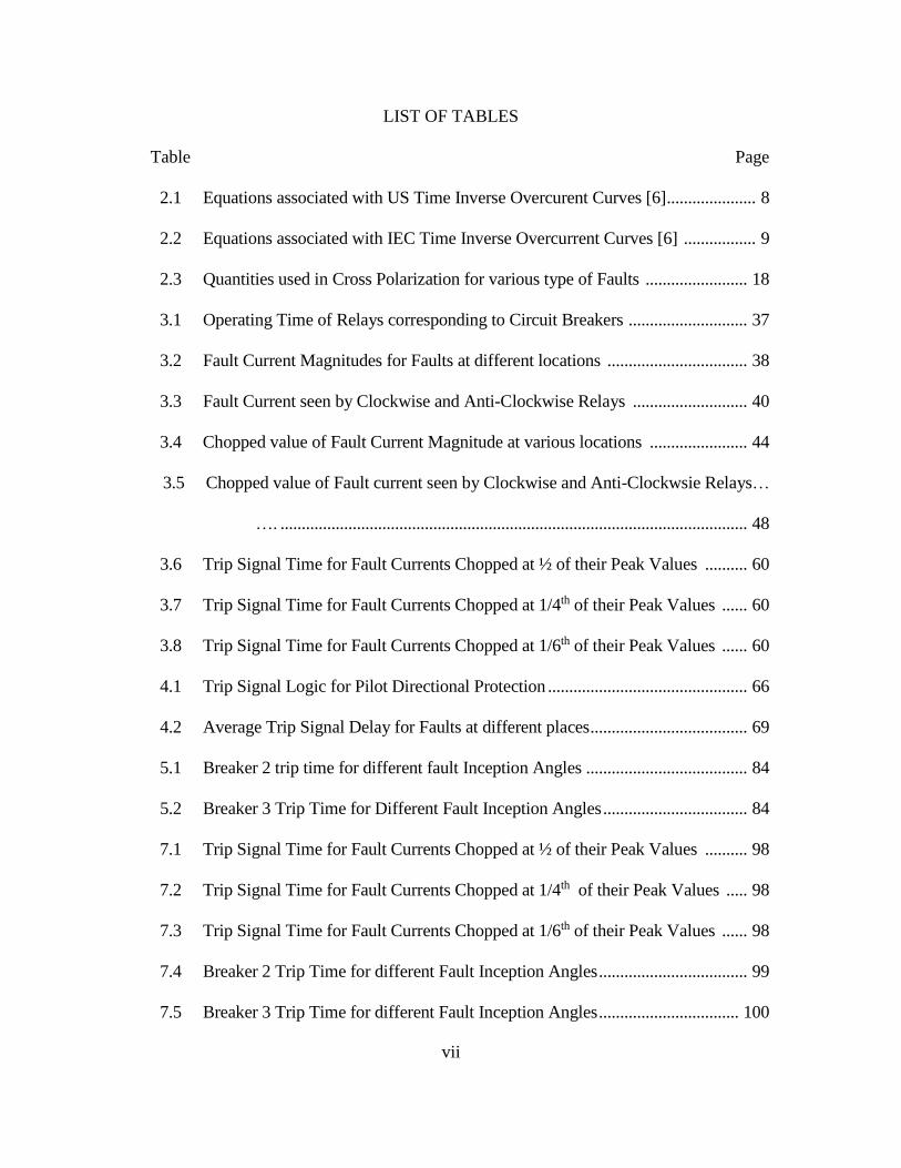
LIST OF TABLES
Table Page
2.1 Equations associated with US Time Inverse Overcurent Curves [6] ..................... 8
2.2 Equations associated with IEC Time Inverse Overcurrent Curves [6] ................. 9
2.3 Quantities used in Cross Polarization for various type of Faults ........................ 18
3.1 Operating Time of Relays corresponding to Circuit Breakers ............................ 37
3.2 Fault Current Magnitudes for Faults at different locations ................................. 38
3.3 Fault Current seen by Clockwise and Anti-Clockwise Relays ........................... 40
3.4 Chopped value of Fault Current Magnitude at various locations ....................... 44
3.5 Chopped value of Fault current seen by Clockwise and Anti-Clockwsie Relays…
…. .............................................................................................................. 48
3.6 Trip Signal Time for Fault Currents Chopped at ½ of their Peak Values .......... 60
3.7 Trip Signal Time for Fault Currents Chopped at 1/4th of their Peak Values ...... 60
3.8 Trip Signal Time for Fault Currents Chopped at 1/6th of their Peak Values ...... 60
4.1 Trip Signal Logic for Pilot Directional Protection ............................................... 66
4.2 Average Trip Signal Delay for Faults at different places ..................................... 69
5.1 Breaker 2 trip time for different fault Inception Angles ...................................... 84
5.2 Breaker 3 Trip Time for Different Fault Inception Angles .................................. 84
7.1 Trip Signal Time for Fault Currents Chopped at ½ of their Peak Values .......... 98
7.2 Trip Signal Time for Fault Currents Chopped at 1/4th of their Peak Values ..... 98
7.3 Trip Signal Time for Fault Currents Chopped at 1/6th of their Peak Values ...... 98
7.4 Breaker 2 Trip Time for different Fault Inception Angles ................................... 99
7.5 Breaker 3 Trip Time for different Fault Inception Angles ................................. 100

viii
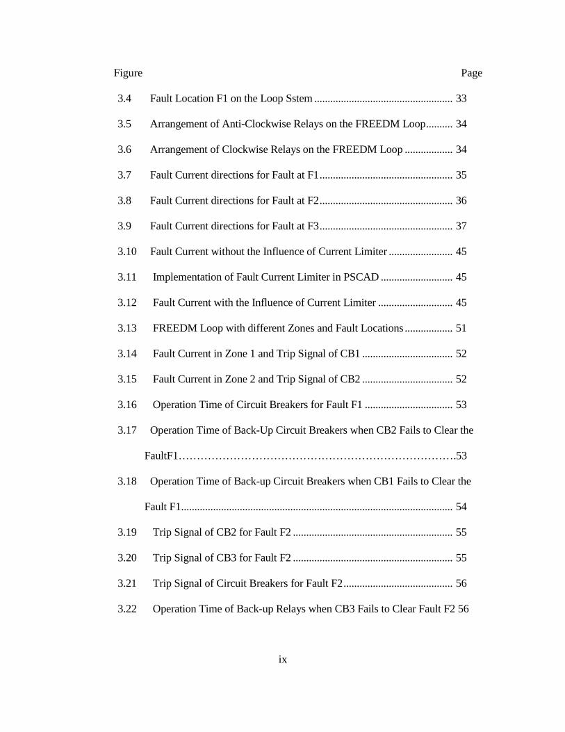
LIST OF FIGURES
Figure Page
1.1 FREEDM Concept Model ........................................................................... 2
1.2 FREEDM Loop ........................................................................................... 3
2.1 Time Inverse Over Current Curve ............................................................. 8
2.2 Operation of Differential Relay without Fault ......................................... 10
2.3 Operaton of Differential Relay for an External Fault .............................. 10
2.4 Operaton of Differential Relay for an Internal Fault ............................... 11
2.5 Pilot Protection Scheme ............................................................................ 13
2.6 Pilot Differential Protection ...................................................................... 15
2.7 Creating Phase Differnce between Voltage and Current using Lead/Lag
Compensator…………………………………………………………... 19
2.8 Sequnce Networks for a Single Line to Ground Fault [24] ..................... 20
2.9 Balanced Phase Voltages [24] .................................................................. 20
2.10 Phase Voltages during SLG Fault on Phase A [24] ................................. 21
2.11 Operating Region and Restraining Region of the Relay [24] .................. 21
2.12 Current Polarization for Forward Fault [24] ............................................ 22
2.13 Current Polarization for Reverse Fault [24] ............................................. 23
2.14 Representation of Synchrophasor [30] ..................................................... 25
2.15 Stable and Un-Stable Region to determine Out of Step Tripping [55] ... 29
3.1 Loop System fed with Multiple Sources .................................................. 31
3.2 Location of Clockwise Relays on the Loop System ................................ 32
3.3 Location of Anti-Clockwise Relays on the Loop System ....................... 32
ix
Figure Page
3.4 Fault Location F1 on the Loop Sstem .................................................... 33
3.5 Arrangement of Anti-Clockwise Relays on the FREEDM Loop .......... 34
3.6 Arrangement of Clockwise Relays on the FREEDM Loop .................. 34
3.7 Fault Current directions for Fault at F1 .................................................. 35
3.8 Fault Current directions for Fault at F2 .................................................. 36
3.9 Fault Current directions for Fault at F3 .................................................. 37
3.10 Fault Current without the Influence of Current Limiter ........................ 45
3.11 Implementation of Fault Current Limiter in PSCAD ........................... 45
3.12 Fault Current with the Influence of Current Limiter ............................ 45
3.13 FREEDM Loop with different Zones and Fault Locations .................. 51
3.14 Fault Current in Zone 1 and Trip Signal of CB1 .................................. 52
3.15 Fault Current in Zone 2 and Trip Signal of CB2 .................................. 52
3.16 Operation Time of Circuit Breakers for Fault F1 ................................. 53
3.17 Operation Time of Back-Up Circuit Breakers when CB2 Fails to Clear the
FaultF1………………………………………………………………….53
3.18 Operation Time of Back-up Circuit Breakers when CB1 Fails to Clear the
Fault F1...................................................................................................... 54
3.19 Trip Signal of CB2 for Fault F2 ............................................................ 55
3.20 Trip Signal of CB3 for Fault F2 ............................................................ 55
3.21 Trip Signal of Circuit Breakers for Fault F2 ......................................... 56
3.22 Operation Time of Back-up Relays when CB3 Fails to Clear Fault F2 56

x
Figure Page
3.23 Operation Time of Back-up Relays when CB2 Fails to Clear Fault F2 . 57
3.24 Trip Signal of CB3 for Fault F3 .............................................................. 57
3.25 Trip signal of CB4 for Fault F3 ............................................................... 58
3.26 Operation Time of Circuit Breakers to Isolate Fault F3 ......................... 58
3.27 Operation Time of Back-up Relays when CB3 Fails to Clear Fault F3 . 59
3.28 Operation Time of Back-up Relays when CB4 Fails to Clear Fault F3 . 59
3.29 Implementing Directional Element in PSCAD ....................................... 62
3.30 Output of Directional Element for a Reverse Fault ................................ 63
3.31 Output of Directional Element for a Forward Fault ............................... 63
3.32 Implementig Clockwise and Anti-Clockwise Relays using a Single Negative
Sequence Directional Element F32 Q………………………………......64
4.1 Radial System with Sources fed from both ends ............................... ....65
4.2 Forward Fault Logic and Reverse Fault Logic of Pilot Directional Protection
………………………………………………………………………….67
4.3 Communication between the Relays ....................................................... 67
4.4 FREEDM Loop with different Zones and Fault Locations .................... 68
4.5 Trip Signal of CB1 for Fault at F1 .......................................................... 70
4.6 Trip Signal of CB2 for Fault at F1 .......................................................... 71
4.7 Trip Signal of CB2 for Fault at F2 .......................................................... 71
4.8 Trip Signal of CB3 for Fault at F2 .......................................................... 72
4.9 Trip Signal of CB3 for Fault at F3 .......................................................... 73
xi
Figure Page
4.10 Trip Signal of CB4 for Fault at F3 .......................................................... 73
4.11 Single Line Diagram of the Hardware Test Bed ..................................... 74
4.12 Mirrored Bit Communication ................................................................. 76
4.13 Experimental Set up for Pilot Directional Protection ............................ 76
4.14 Trip Signal from AcSELerator Quickset Software of SEL ................... 77
5.1 7 Load FREEDM Systesm developed by MS&T ................................... 78
5.2 7 Load FREEDM System Modeled on RTDS ........................................ 79
5.3 Trip Signal of CB2 for a 3 Phase to Ground Fault ................................. 80
5.4 Voltage seen by Relay during 3 Phase Fault ........................................... 80
5.5 Trip Signal of CB3 for a 3 Phase to Ground Fault ................................. 81
5.6 File Generated from AcSELerator Quickset for a 3 Phase Fault ........... 82
5.7 Trip Signal of CB2 for a ABC-LLL Fault .............................................. 82
5.8 Voltage seen by Relay for a ABC-LLL Fault ......................................... 83
5.9 Trip Signal of CB3 for a ABC-LLL Fault .............................................. 83
6.1 FREEDM System showing PMU Location ........................................... 86
6.2 Logic to Detect an Event Using Synchrophasor Measurements ........... 86
6.3 Voltage Phase difference of Phase A between PMU 1 and PMU 2 for a SLG
Fault…..………………………………..……………………………….87

xii
Figure Page
6.4 Absolute Value of Voltage Phase differene of Phase A between PMU 1 and
PMU 2 for a SLG Fault…………………………………………………88
6.5 Voltage Phase difference of Phase A between PMU 2 and PMU 3 for a SLG
Fault……..…………………………………………………………….. .88
6.6 Voltage Phase difference of Phase A between PMU 3 and PMU 4 for a SLG
Fault ………...…………………………………………………………89
6.7 Voltage Phase difference of Phase A between PMU 4 and PMU 1 for a SLG
Fault……………………………………………………………………..89
6.8 Decrease in Fault Current due to the Isolation of Fault
…………………………………………………………………………..90
6.9 Voltage phase difference of Phase A between PMU 1 and PMU 2 for ABC-
GFault…………………………………………………………………...90
6.10 Voltage Phase difference of Phase B between PMU 1 and PMU 2 for
ABC-GFault…………………………………………………………………
…………………………………………………………………………..91
6.11 Voltage Phase difference of Phase C between PMU 1 and PMU 2 for
ABC-
GFault……………………………………………………………………91
6.12 Trip Signal Generated from PMU 1 and PMU 2 Data…………………
…………………………………………………………………………...92

xiii
Figure Page
6.13 Voltage Phase difference of Phase A between PMU 2 and PMU 3 for ABC
GFault……………………………………………………………………92
6.14 Voltage Phase difference of Phase A between PMU 3 and PMU 4 for
ABCG Fault……………………………………………………………...93
6.15 Voltage Phase difference of Phase A between PMU 4 and PMU 1 for
ABCGFault………………………………………………………………93
6.16 Hardware Set up for PMU based
Protection………………............................................................................95
6.17 Single Line Diagram of 3 Phase Test Bed used for Hardware
Implementation……...…………………………………………………..96
6.18 Graph Obtained from Synchro Vector
Processor………………………………………………………………...96

xiv
NOMENCLATURE
FREEDM Future Renewable Electric Energy delivery and Management
SST Solid State Transformer
AC Alternating Current
DC Direct Current
TDS
FCL
RTDS
PMU
Time Dial Settings
Fault Current Limiter
Real Time Digital Simulator
Phasor Measuring Unit
TIDOC Time Inverse Directional Overcurrent
SCDR Symmetrical Component Distance relay
FFL Forward Fault Logic
RFL Reverse Fault Logic
DG Distributed Generation
PSAT Power System Analysis Tool
CT Current Transformer
PT Potential Transformer
UPFC Unified Power Flow Controller
SLG Single Line to Ground
ABC-G Three Phase to ground
ABC-LLL Three Phase Short Circuit

1
CHAPTER 1
INTRODUCTION TO THE FREEDM SYSTEM
1.1 Overview
Burning out the fossil fuels for power generation and increased global warming
caused by excessive 𝐶𝑂2 emissions have become a greater concern for the US government
[1]. In order to prevent the excessive exhaustion of natural resources by power companies
without having a reduction in power generation, federal government passed a strict law to
include the renewable sources in total power generation. In addition to the federal laws,
ambitious renewable portfolio standards (RPS) and advancements in technology have led
to an extensive increase in renewable integration in the US power industry. Renewable
integration has become a dominant area of research both at the academic and industry level.
Integrating wind, solar PV, bio-fuel and others to the existing power system at the
distribution level would create a wide variety of technical difficulties. In spite of the
advancement in power electronics, energy storage devices and communication there are
still few problems like grid reliability, price of electricity and others that are to be taken
care of while integrating renewable resources.
FREEDM (Future Renewable Electric Energy Delivery and Management) is an
initiative by the National Science Foundation (NSF) to overcome the above mentioned
problems. The solution to solve the energy crisis is not solely the renewable energy but the
equipment involved in delivering the energy and maintaining the system operating
conditions [1]. Due to the presence of local distributed generation, the power flow in the
system is bi-directional and the conventional protection methods may face the problem of

2
false tripping. Due to the presence of power electronic converters and devices (power
electronic based fault current limiters and solid state transformer) the behavior of fault
current is different from a conventional distribution system [2], [3].
1.2 FREEDM system
FREEDM system was developed as a smart grid system with a motivation to
include renewable sources into the existing power grid. FREEDM system is a culmination
of high bandwidth digital communication, power electronics and digital communication
[1]. It replaces conventional transformer of 60 Hz with solid state transformer (SST)
incorporating bidirectional power flow. Solid state transformer is a package of cascaded
rectifier, dual active bridge converter and inverter. It has an input of 7.2 kV AC and output
of 120 V AC single phase, 208 V AC (3 phase) and 400 V DC. All the DC loads, distributed
generation and energy storage devices are connected to the DC link and AC loads are
connected to the AC output.
Figure 1.1 FREEDM concept model

3
To demonstrate the advancement done in FREEDM project, a 1 MW green energy
smart hub is under development. The proposed FREEDM loop allows consumers to plug
and play energy sources or storage devices from anywhere on the loop [1]. To provide
effective power flow, power distribution and fault detection; intelligent energy
management (IEM) and intelligent fault detection (IFD) control schemes are incorporated
in the FREEDM system. Following Figure 1.1 shows the schematic layout of the FREEDM
system and Figure 1.2 shows the single line diagram of the FREEDM system. The
FREEDM loop is connected to grid and in the case of grid failure, the loop can operate
independently.
Figure 1.2 FREEDM loop
1.3 Objectives of the research
The power flow in the FREEDM system is bi-directional due to the presence of
distributed generation (DG) and the conventional protection methodologies must be
modified accordingly to detect fault conditions and prevent false tripping. The solid state
transformers (SST) have self-protection, which shuts them down during faults when the
4
voltage goes below a certain threshold voltage and it can be adjusted. In the case of a loop
system during faults, the voltage of the entire loop plummets to zero or typically a low
value. In such a scenario all the SST’s connected to the loop will shut down due to its self-
protection. Hence, it is important to isolate the faulted part of the network from the rest of
the system to prevent the shutdown for SST’s. Pilot differential protection was developed
as a solution to the above mentioned problem by former ASU FREEDM students. It was
able to detect faults within quarter of a cycle but it suffered from the problem of
communication [4]. Ethernet cable was used as the communication medium to transfer the
sampled signals from the current transformers to the central processor. The central
processor analyzes the sampled current signals, generates the trip depending up on the
system conditions and sends the trip signal back to the breaker. The entire communication
is carried out by the ethernet cable which is practically not feasible to implement for longer
distances (7 mile to 10 mile) because of latency and economical factors. A solution to the
above communication problem is suggested in this thesis as a part of FREEDM research
work.
A protection method is developed that could protect looped systems with multiple
sources without using any sort of communication. Directional relays with time inverse
over current characteristics are coordinated affectively to detect and sectionalize the
fault location without affecting the healthy part of the system. This serves as a reliable
back-up protection system when the communication system fails.
A new pilot protection method is developed using the commercial SEL relays which
uses the direction of fault currents to locate the fault. The communication is done using
fiber-optic cables and the only data needed to be transferred between the relays is the

5
fault location which is transferred in the form of digital bits. Simulation, hardware
implementation and real time digital system (RTDS) validation is explained in the
thesis.
A protection method is suggested monitoring the sychrophasor measurements, voltage
of the system and current during faults.
1.4 Organization of the thesis
Chapter 2 presents the existing over current protection, differential pilot protection
schemes and use of synchrophasor data in power system monitoring and control. Standard
method of implementing pilot protection scheme is explained. Chapter 3 presents the
development of time inverse directional over current and PSCAD simulation. Chapter 4
presents the development of pilot directional protection, PSCAD simulation, hardware
implementation and validation of the protection scheme on RTDS system. Chapter 5
presents the validation of pilot directional scheme over the FREEDM system on real time
digital simulator (RTDS). Chapter 6 presents the development of PMU based protection
and hardware implementation. Chapter 7 presents conclusions, problems faced during
hardware implementation and future work.
Appendix A presents the graphs showing trip signal of breakers, fault current
magnitude and variation in system voltage for different faults at various fault angles.
Appendix B presents the code used in Synchro Vector Processor (SVP) configurator used
to communicate with the SVP SEL 3378. Appendix C presents the generator data and
system data used in real Time Digital Simulator (RTDS) simulation. Appendix D presents

6
the power flow information used to determine the voltage phase angle difference during
maximum power flow.
7
CHAPTER 2
LITERATURE REVIEW
2.1 Over current protection
Instantaneous Over current protection
Relay operates when current value goes beyond a preset threshold value.
Instantaneous over current protection is most commonly used in distribution systems and
equipment as a protection against short circuits and high fault currents.
Definite time over current protection
Relays operate with a definite preset time delay when current value goes beyond a
threshold value. It’s operation is independent of magnitude of fault current above the
threshold value.
Inverse time over current relays
Relays operate when the current value goes beyond a pick up current value. The
time of operation is inversely proportional to the magnitude of fault current. High fault
currents operate the relay faster than lower value of fault currents. It has two settings:
(i) Time dial settings (TD)
(ii) Current pick up settings
Figure 2.1 shows the time inverse over current characteristics with time dial settings
and current pick up values.

8
Figure 2.1 Time inverse over current curve [5]
These relays are classified into different types based on their operating time and
reset time. Table 2.1 and Table 2.2 describe the standard inverse time characteristic
equations of the relays as per IEEE C37.112-1996 standards and IEC standards [5], [6].
Table 2.1 Equations associated with US curves [6]
S.no Curve Type Operating Time Reset Time
1 U1 (Moderately Inverse) 𝑡𝑝 = 𝑇𝐷. (0.0226
+0.0104
𝑀0.02 − 1)
𝑡𝑟 = 𝑇𝐷. (1.08
1 − 𝑀2)
2 U2 (Inverse) 𝑡𝑝 = 𝑇𝐷. (0.180 +
5.95
𝑀2 − 1) 𝑡𝑟 = 𝑇𝐷. (
5.95
1 − 𝑀2)
3 U3 (Very Inverse) 𝑡𝑝 = 𝑇𝐷. (0.0963 +
3.88
𝑀2 − 1) 𝑡𝑟 = 𝑇𝐷. (
3.88
1 − 𝑀2)
4 U4 ( Extremely Inverse) 𝑡𝑝 = 𝑇𝐷. (0.0352 +
5.67
𝑀2 − 1) 𝑡𝑟 = 𝑇𝐷. (
5.67
1 − 𝑀2)
5 U5 (Short-Time Inverse) 𝑡𝑝 = 𝑇𝐷. (0.00262
+0.00342
𝑀0.02 − 1)
𝑡𝑟 = 𝑇𝐷. (0.323
1 − 𝑀2)

9
Table 2.2 Equations associated with IEC curves
S.no Curve Type Operating Time Reset Time
1 C1 (Standard Inverse) 𝑡𝑝 = 𝑇𝐷. (
0.14
𝑀0.02 − 1) 𝑡𝑟 = 𝑇𝐷. (
13.5
1 − 𝑀2)
2 C2 (Very Inverse) 𝑡𝑝 = 𝑇𝐷. (
13.5
𝑀2 − 1) 𝑡𝑟 = 𝑇𝐷. (
47.3
1 − 𝑀2)
3 C3(Extremely Inverse) 𝑡𝑝 = 𝑇𝐷. (
80
𝑀2 − 1) 𝑡𝑟 = 𝑇𝐷. (
80
1 − 𝑀2)
4 C4(Long time Inverse) 𝑡𝑝 = 𝑇𝐷. (
120
𝑀 − 1) 𝑡𝑟 = 𝑇𝐷. (
120
1 − 𝑀)
5 C5(Short-Time Invese) 𝑡𝑝 = 𝑇𝐷. (
0.05
𝑀0.04 − 1) 𝑡𝑟 = 𝑇𝐷. (
4.85
1 − 𝑀2)
Over current differential protection
Over current differential protection is based on the Kirchhoff’s first law, “the sum
of the current flowing into a node must be equal with the sum of the currents leaving the
same node.” Over current differential scheme is applied to various parts of power system
equipment such as transformer, bus-bar, generators with small and moderate kVA, motors,
transmission lines and other parts of the power system [7]. In the case of an external fault
to a transmission line or a transformer, the sum of the current entering and leaving the
element would be equal. However, in the case if an internal fault, current will be sinking
into the element and summation of the current entering into the element will not be equal
to the current leaving the element.

10
Operating principle of differential relay
The current flowing through the operating coil is the difference of the input entering
current and output leaving current. During the normal operation without any fault, both the
entering current and leaving currents are equal. So the current in the operating coil is zero.
Figure 2.2 shows the arrangement for differential protection of an element in the power
system.
Figure 2.2 Operation of differential relay without fault [9]
During an external fault to the protected unit, the current in the operating coil is still
zero as the current entering equals the current leaving the unit. Figure 2.3 shows the
operation of a differential relay for an external fault.
Figure 2.3 Operation of differential relay for an external fault [9]

11
But for an internal fault current sinks into the protected unit and the current in the
operating coil goes higher than the pickup value and results in a trip signal generation [8],
[9]. Figure 2.4 shows the operating current activating the relay trip coil during an internal
fault.
Figure 2.4 Operation of differential relay for an internal fault [9]
2.2 Pilot protection
The advancement of serial and wireless communication created a significant
improvement in the usage of communication link in protection schemes. Pilot protection
scheme employs communication to use the information from local relay and remote relay
to effectively make decision for the trip signal generation. Fault clearing time is very
important in long transmission lines operating at high voltage or extra high voltage. Any
delays in the trip signal could cause severe stability problems to the network. High fault
currents created in transmission lines could cause severe damage to the equipment. Hence
it is vital to clear the fault as soon as possible and pilot protection helps to achieve the fast
means of trip generation [10]. The communication in pilot protection schemes is usually

12
analog or digital transmitting at power frequencies or higher frequencies. Following are
few modes of existing communication [11].
1) Audio frequencies ranging from 20-20000 Hz,
2) Power carrier frequency in the range from 30 to 600 kHz,
3) Radio frequencies ranging from 10kHz to 100,000MHz,
4) Microwave frequency bands loosely applied to radio waves from 1000 MHz,
5) Visible light frequencies with nominal wavelength range of about 0.3μm - 30μm.
Pilot protection scheme is classified in following types depending on the quantities
transferred and compared.
i. Unit pilot protection schemes
In this protection scheme only the analog quantities such as amplitude or phase are
compared over the communication link between the relays [11].
ii. Non-unit pilot protection schemes
In this protection scheme the logical states related to fault information of the
protection algorithm is transferred and compared over the communication channel between
the relays or in a central processor to generate trip signal [11].
Unit protection schemes
a) Longitudinal differential Scheme or pilot differential scheme
Pilot differential scheme is based on the principle of over current differential
protection. The comparison of current signals and decision making takes place over the
communication link. The relays gather the current magnitude and phase angle information
13
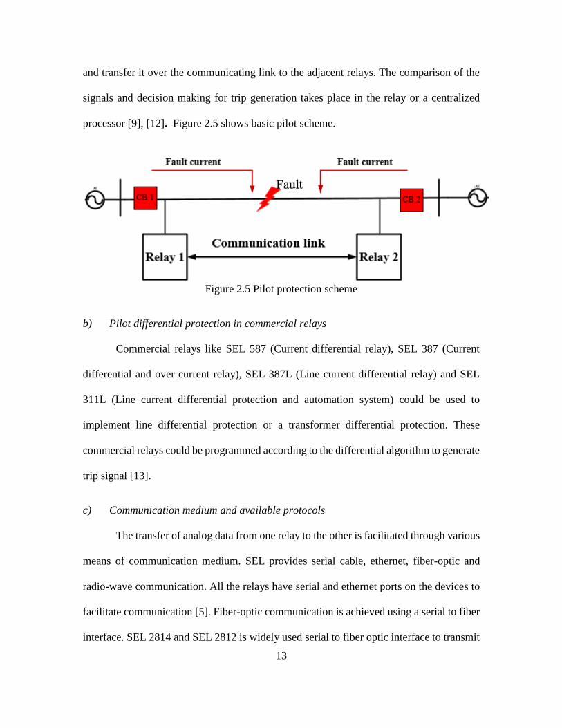
and transfer it over the communicating link to the adjacent relays. The comparison of the
signals and decision making for trip generation takes place in the relay or a centralized
processor [9], [12]. Figure 2.5 shows basic pilot scheme.
Figure 2.5 Pilot protection scheme
b) Pilot differential protection in commercial relays
Commercial relays like SEL 587 (Current differential relay), SEL 387 (Current
differential and over current relay), SEL 387L (Line current differential relay) and SEL
311L (Line current differential protection and automation system) could be used to
implement line differential protection or a transformer differential protection. These
commercial relays could be programmed according to the differential algorithm to generate
trip signal [13].
c) Communication medium and available protocols
The transfer of analog data from one relay to the other is facilitated through various
means of communication medium. SEL provides serial cable, ethernet, fiber-optic and
radio-wave communication. All the relays have serial and ethernet ports on the devices to
facilitate communication [5]. Fiber-optic communication is achieved using a serial to fiber
interface. SEL 2814 and SEL 2812 is widely used serial to fiber optic interface to transmit

14
the signals over fiber-optic cables. Two sets of fibers should be used to transmit and receive
the signals. Selection of fiber optic transceivers must be done basing on how long the data
must be transferred. Radio wave communication is achieved using the SEL-3031 module.
It could generate waves up to 915 MHz with point to point and point to multiple
point operation modes [13]. All the communication ports could be accessed by various
protocols. Following are the communication protocols present in the SEL relays:
1) DNP 3
2) Modbus
3) SEL fast messages
4) Mirrored bit communication
5) Plain ASCII
Protection method
The analog current signals are transferred with the time stamp using a synchronized
GPS clock. Instantaneous current values and current phase angles are transferred over the
available communication cables using any of the above mentioned protocols [14], [15].
Figure 2.6 shows the schematic for pilot differential protection.
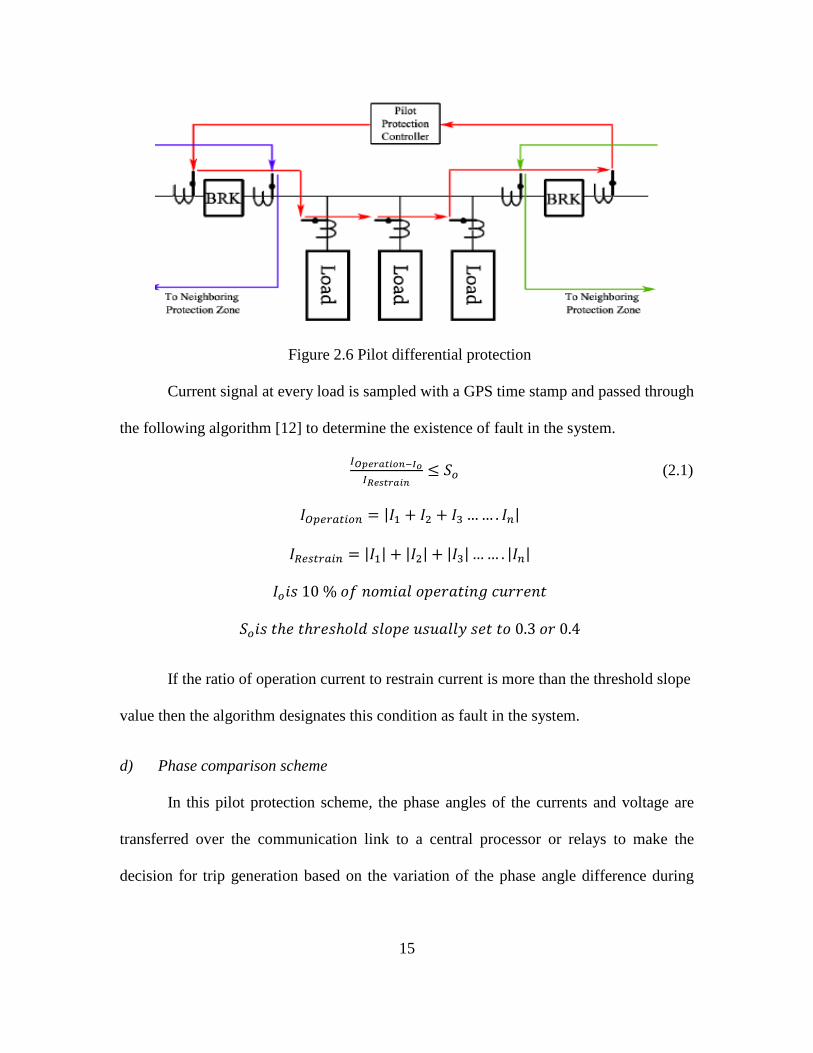
15
Figure 2.6 Pilot differential protection
Current signal at every load is sampled with a GPS time stamp and passed through
the following algorithm [12] to determine the existence of fault in the system.
𝐼𝑂𝑝𝑒𝑟𝑎𝑡𝑖𝑜𝑛−𝐼𝑜
𝐼𝑅𝑒𝑠𝑡𝑟𝑎𝑖𝑛≤ 𝑆𝑜 (2.1)
𝐼𝑂𝑝𝑒𝑟𝑎𝑡𝑖𝑜𝑛 = |𝐼1 + 𝐼2 + 𝐼3 … … . 𝐼𝑛|
𝐼𝑅𝑒𝑠𝑡𝑟𝑎𝑖𝑛 = |𝐼1| + |𝐼2| + |𝐼3| … … . |𝐼𝑛|
𝐼𝑜𝑖𝑠 10 % 𝑜𝑓 𝑛𝑜𝑚𝑖𝑎𝑙 𝑜𝑝𝑒𝑟𝑎𝑡𝑖𝑛𝑔 𝑐𝑢𝑟𝑟𝑒𝑛𝑡
𝑆𝑜𝑖𝑠 𝑡ℎ𝑒 𝑡ℎ𝑟𝑒𝑠ℎ𝑜𝑙𝑑 𝑠𝑙𝑜𝑝𝑒 𝑢𝑠𝑢𝑎𝑙𝑙𝑦 𝑠𝑒𝑡 𝑡𝑜 0.3 𝑜𝑟 0.4
If the ratio of operation current to restrain current is more than the threshold slope
value then the algorithm designates this condition as fault in the system.
d) Phase comparison scheme
In this pilot protection scheme, the phase angles of the currents and voltage are
transferred over the communication link to a central processor or relays to make the
decision for trip generation based on the variation of the phase angle difference during

16
faults. Care must be taken when implementing this protection method, as the change in
network configuration would result a change of the phase angles [16].
Non-unit pilot protection schemes
a) Distance scheme
Communication in distance protection can eliminate the time delays that occur to
detect the existence of faults in zone 2 or zone 3. Local relays could communicate to the
remote relays in long transmission lines to guarantee the fault and it could speed up the
operation. Permissive under reaching and permissive over reaching are the popular pilot
schemes used.
2.3 Detecting the direction of fault current
Above explained pilot methods transfer analog signal data with a time stamp. The
implementation of the above methods requires a huge data storage and data handling
capacity by the communication system. One solution to the above problem is to use the
direction of fault current to locate the fault. Following explains the different methods
developed in the literature to determine the fault current direction.
The deviation in the voltage and current from normal steady state condition due to
fault was used to determine the power direction. But there is a chance for the protection
strategy to mis-trip if it fails to distinguish in between the switching transients and lightning
with fault conditions [17]. A new method was developed using the superimposed sequence
currents (vector ratio of positive sequence and negative sequence currents) to determine
the faulty phase and fault current direction [18]. It requires a high speed phase selector in-
order to determine the fault phase by comparing the sequence components. The evolution
17
of microprocessor relays simplified the work of protection engineers to find the sequence
components. Scalar product of incremental in voltage and current is used to determine the
fault current direction [19]. Following section describes different methods used to
implement the directional relay.
i. Conventional method
In electro-mechanical relays the direction of fault is determined depending on the
direction of torque produced. The torque equation for the electro-mechanical relay is shown
below.
𝑇 = 𝑉𝑝𝑜𝑙 . 𝐼𝑜𝑝. cos( − 𝑉𝑝𝑜𝑙 − 𝐼𝑜𝑝) (2.2)
𝐼𝑜𝑝 is the current of the faulted phase
Positive torque results from forward faults and negative torque from reverse faults.
Jeff Roberts and Armando Guzmán demonstrated that equation 2 is computationally
efficient to determine the fault direction in microprocessor based relays [20].
𝑇 = 𝑅𝑒[−𝑉𝑝𝑜𝑙 . 𝐼𝑝𝑜𝑙] (2.3)
There is no single approach that could work for all faults and all line configurations.
Therefore microprocessor based relays use multiple algorithms in combination to
determine fault location. Polarizing signals are a reference for comparing the operating
quantities that are affected during fault. They help to determine the direction of fault to a
relay (forward or reverse). Polarizing signals should be present at all the times irrespective
of fault type and location.

18
ii. Cross polarizing
During a single phase to ground fault the 𝑉𝑃𝑁 (phase to neutral voltage) goes to zero
and the corresponding fault current lags the voltage by a large angle due to the high
reactance of line. This prevents the relay from detecting the correct fault direction. To
resolve the low voltage issue the voltage of unaffected phases is used. Phase to phase
voltages (VBC and IA) are used to detect the direction of fault [21].
Table 2.3 Cross polarizing table
Faulted phase Operating Quantity Polarizing Quantity
A Ia Va-Vb
B Ib Vc-Va
C Ic Va-Vb
AB Iab -j.Vc
BC Ibc -j.Va
CA Ica -j.Vb
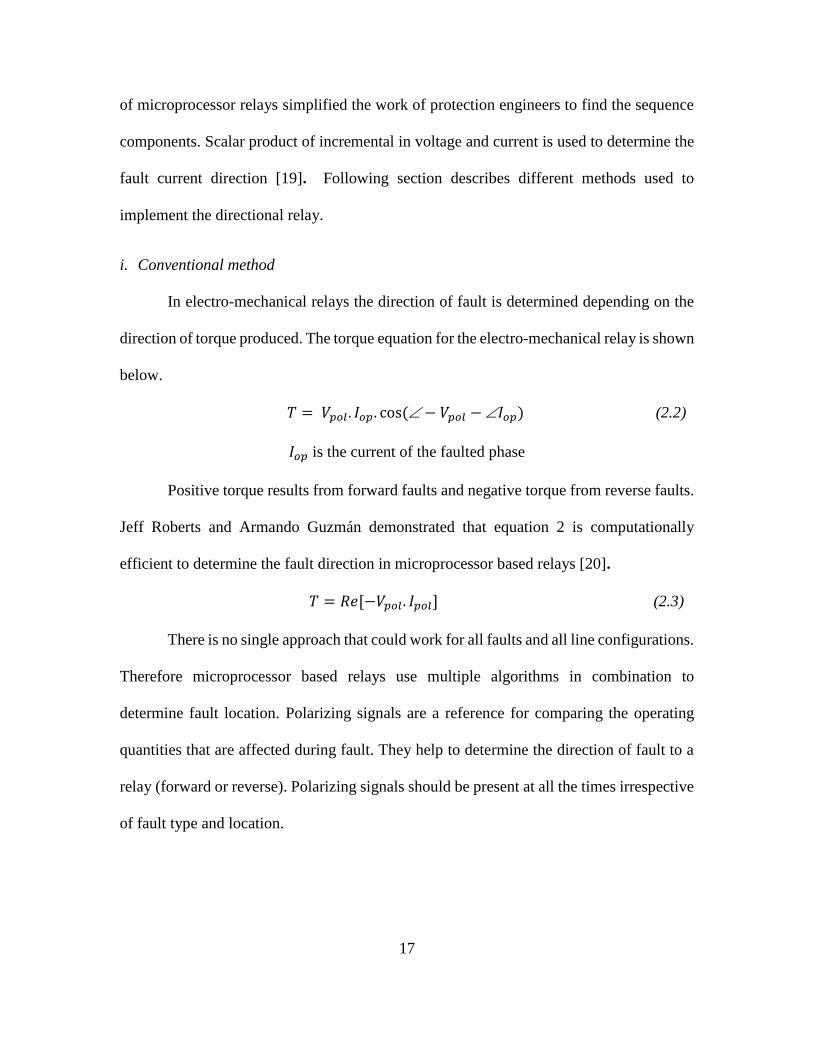
To overcome the backdrop due to high lagging current, the voltage of the relays in
the algorithm is passed through a lead or lag compensator so that the relays could detect
the fault. Figure 2.7 shows the compensation of phase-phase voltage [22]. Every relay
manufacturer has its own voltage compensation algorithm to detect the fault.
19
Figure 2.7 creating phase angle difference between voltage and current [21]
The development of micro-processor relays enabled protection engineers to use
sequence components for developing new methods to determine the direction of fault
current. Zero-sequence voltage polarization, zero-sequence current polarization, negative
sequence polarization are the popular methods developed from sequence components.
iii. Zero sequence voltage polarization
Zero sequence voltage polarization measures the angle between the zero sequence
voltage and residual current to determine the direction of fault current. Residual current is
obtained from summation of individual phase currents and is usually obtained from the
current transformer installed in the neutral wire. The residual current and the zero sequence
voltage are displaced by an angle of line impedance and source impedance [23], [24].
Figure 2.8 represents the sequence network of a system with sources 𝐸𝑆 and 𝐸𝑅 supplied
from both the ends. The fault location on the line is at a distance 𝑚. 𝑍𝐿𝑖𝑛𝑒 where m is the
per unit length of the line.

20
Figure 2.8 Sequence networks for a single line to ground fault [24]
Because of the reactive nature of the transmision line and the fault impedance being
reactive the torque developed is maximum when current lags the residual voltage by an
angle called “Maximum Torque Angle (MTA).”
32𝑉𝑇 = |𝑉0|. |𝐼𝑅|. [cos(∠ − 𝑉0 − (∠𝐼𝑅 + 𝑀𝑇𝐴))] (2.4)
The torque value is positive for a forward fault and negative for a reverse fault. The
directional elements also require minimum voltage and current for their operation to
produce torque value. Figure 2.9 shows the balanced phase angles of a system.
Figure 2.9 Balanced phase voltages [24]
21
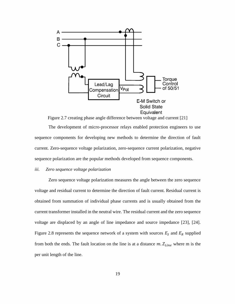
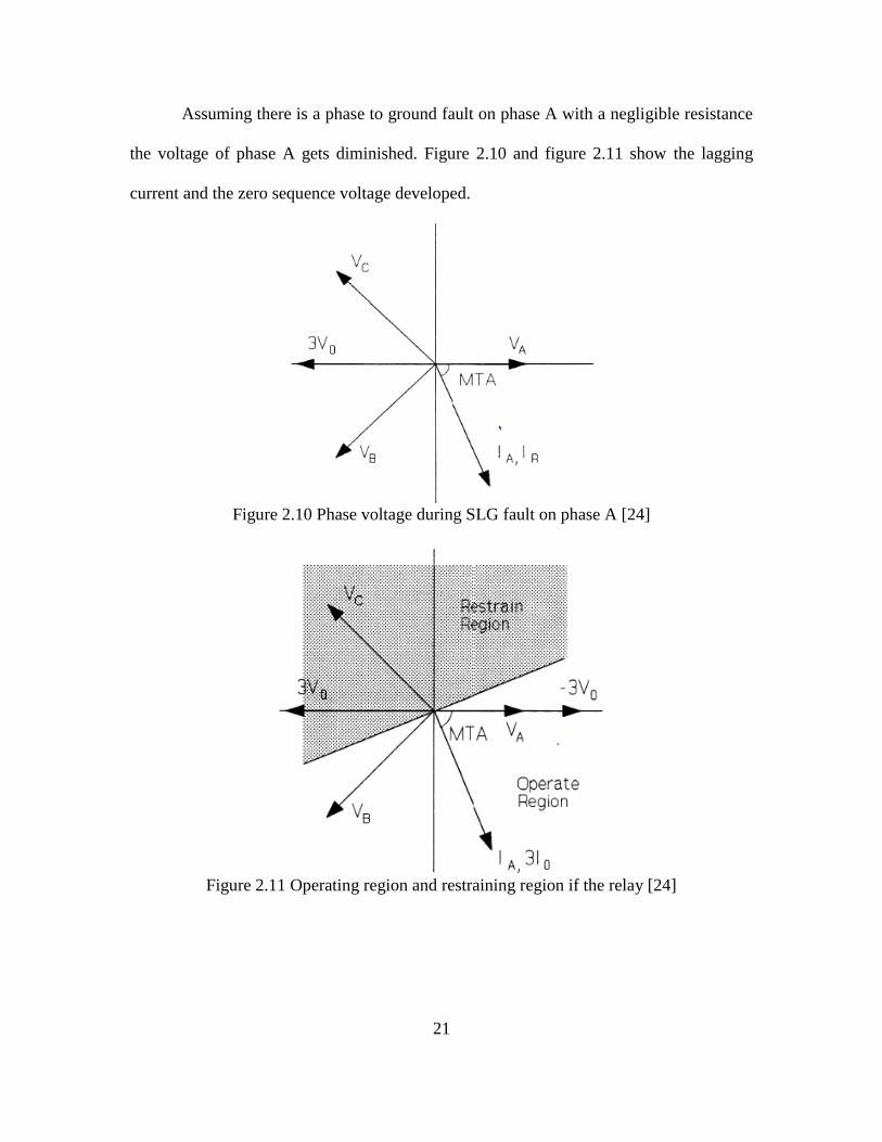
Assuming there is a phase to ground fault on phase A with a negligible resistance
the voltage of phase A gets diminished. Figure 2.10 and figure 2.11 show the lagging
current and the zero sequence voltage developed.
Figure 2.10 Phase voltage during SLG fault on phase A [24]
Figure 2.11 Operating region and restraining region if the relay [24]

22
iv. Zero Sequence Current Polarization
For few fault conditions the residual voltage developed is not sufficient to polarize
the relay. To overcome such scenarios, the neural current of a transformer (near to the
relay) with a grounded neutral can be used as a polarizing quantity [24]. For a forward
fault, the residual current seen by the relay and the neutral current are in the same direction.
For a reverse fault, the direction of the residual current is in opposite direction to that of
the neutral current.
32𝐼𝑇 = |𝐼𝑝𝑜𝑙|. |𝐼𝑅|. cos(∠𝐼𝑃𝑜𝑙 − ∠𝐼𝑅) (2.5)
From the torque equation, the maximum torque is developed when the polarizing
current and the residual current are in phase. One thing that has to be taken care of when
using this technique is the direction of polarizing current has to be same for all faults. If
the direction of the polarizing current is not the same then this technique cannot be used.
Figure 2.12 shows the direction of fault current and polarizing current for a forward fault.
Figure 2.12 Current polarization for forward fault [24]
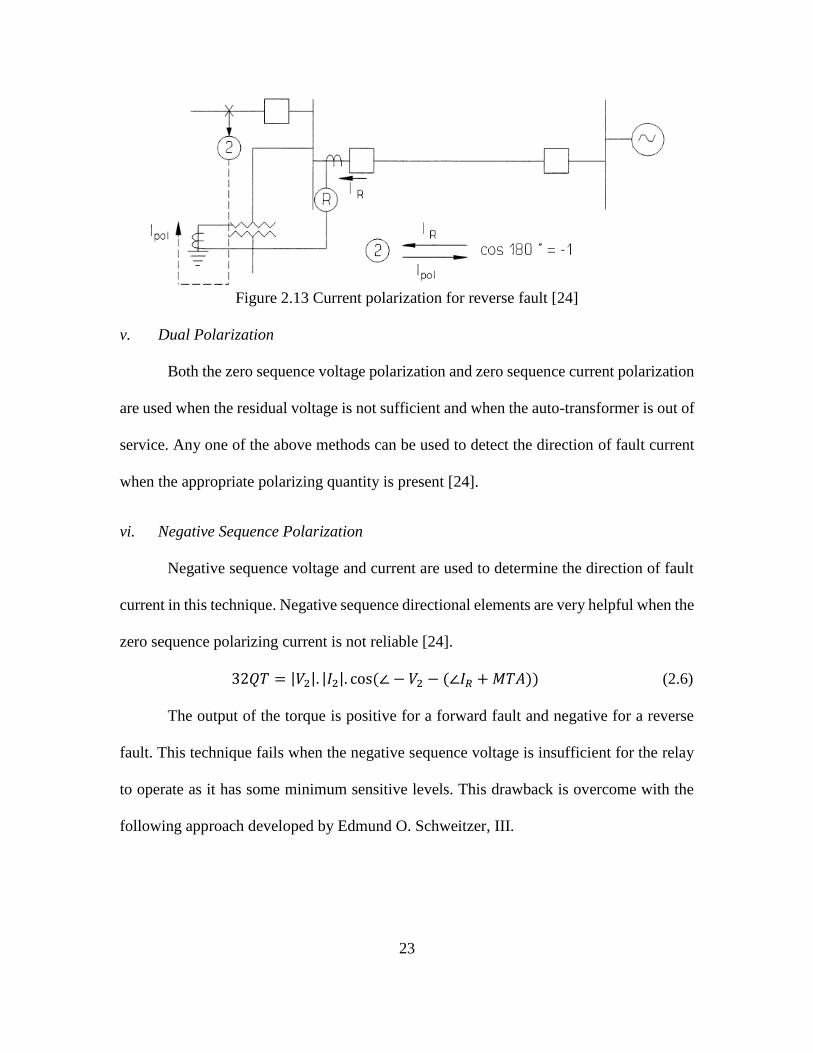
Figure 2.13 shows the direction of fault current direction and polarizing current for
a reverse fault.
23
Figure 2.13 Current polarization for reverse fault [24]
v. Dual Polarization
Both the zero sequence voltage polarization and zero sequence current polarization
are used when the residual voltage is not sufficient and when the auto-transformer is out of
service. Any one of the above methods can be used to detect the direction of fault current
when the appropriate polarizing quantity is present [24].
vi. Negative Sequence Polarization
Negative sequence voltage and current are used to determine the direction of fault
current in this technique. Negative sequence directional elements are very helpful when the
zero sequence polarizing current is not reliable [24].
32𝑄𝑇 = |𝑉2|. |𝐼2|. cos(∠ − 𝑉2 − (∠𝐼𝑅 + 𝑀𝑇𝐴)) (2.6)
The output of the torque is positive for a forward fault and negative for a reverse
fault. This technique fails when the negative sequence voltage is insufficient for the relay
to operate as it has some minimum sensitive levels. This drawback is overcome with the
following approach developed by Edmund O. Schweitzer, III.

24
vii. Negative Sequence impedance technique
Relay calculates the apparent negative sequence impedance between the faults and
relay location. It overcomes the problem of weak polarizing quantity caused by low
voltage source (weak in-feed) behind the relay. For faults at remote location, the magnitude
of negative sequence voltage seen by the relay might be very less. To overcome this
problem a compensating quantity is added that boosts the negative sequence voltage. The
compensating quantity is added to V2 for forward faults and subtracted for reverse faults.
𝑍2 =𝑅𝑒[𝑉2.(𝐼2.1θ)∗]
𝑅𝑒[(𝐼2.1θ).(𝐼2.1θ)∗]=
𝑅𝑒[𝑉2.(𝐼2.1θ)∗]
𝐼22 (2.7)
The calculated 𝑍2 is compared to the forward and reverse impedance thresholds to
determine the fault location. If the calculated impedance is less than the forward threshold
impedance then he fault is forward, if 𝑍2 is greater than reverse threshold impedance then
the fault is reverse. If the calculated impedance 𝑍2 lies within forward threshold impedance
and reverse threshold impedance then there is no fault [25]. This approach is not affected
by the zero-sequence mutual coupling between the parallel lines [26], [27], [28].
2.4 Application of synchrophasors in power system monitoring, protection and control
Power system is a vast electrical network spread through the geographical
locations. Electricity is transferred from the generation site to hundreds of miles over
various locations. It is highly essential to monitor the states of power system to effectively
monitor the operation and control of power delivery. Voltage magnitude, voltage phase
angle, current magnitude, current phase angle and frequency are the important states that
should be monitored. If these values are known active and reactive power in the system
can be calculated using the line impedance.

25
Due to the vast separation between different electrical nodes it was difficult to
estimate these states. However, with the development of synchrophasor measurements the
above challenge could be handled effectively with good communication technology. The
device capable of measuring synchrophasors is called phasor measuring unit (PMU). A
phasor is a complex number that represents magnitude and phase angle of a waveform at
specified frequency at a specific point in time [29]. Figure 2.14 shows the phasor
representation of a sinusoidal waveform.
Figure 2.14 Representation of synchrophasor [30]
GPS synchronized time stamp is used as a reference for the measurement of
phasors. The widely accepted standards for measuring and communicating the time
stamped signals are defined in IEEE C37.118 standards.
IEEE C37.118 standards
These standards specify the frequency and rate of change of frequency under all
operating conditions. It specifies only about the measurements but not about the hardware,
software and the method for computing these phasors.

26
The standard mentions about two classes of performance: M and P. In the M class,
phasors are passed through an anti-aliasing filter and are used in the applications where the
fast transfer of signals is not needed. In the P-class, the signals are not passed through any
sort of filter and are typically intended to use for protection application. The standard also
talks about the accuracy of the measurements in terms of Total Vector Error (TVE). The
maximum allowable phase angle error is 0.57 degrees [31], [32], [33].
History of PMU development and its wide area applications
The blackout of 1965 in North-East United States resulted in wide areas of research
to improve the secured operation of power system. The idea of static state estimator was
introduced to have a wide area monitoring of the system. Due to the technological
limitations at that point of time, an approximate state estimation is evaluated known as
quasi-steady state using the wide area inputs [34].
Computer relaying was first introduced as a research field in 1960’s to detect the
fault location. This research led to the development of symmetrical component distance
relay (SCDR) for protecting high voltage transmission lines [35], [36]. PMU was
developed from the idea of SCDR. It was first developed in 1988 by Dr. Arun G. Phadke
and Dr. James S. Thorp at Virginia Tech and the phasor calculation is based on the paper
presented by Charles Proteus Steinmetz about using the mathematical description of
complex numbers in electrical engineering [37]. Since then, PMU’s have become a wide
area of research for their application in monitoring, protection and control.
Paper [38] presents a method to use current differential algorithm along with wide
area measurements to secure the operation of distance relays during power swing blocking.

27
A new algorithm is presented in paper [39] to determine the fault location without installing
PMU at every bus location. It uses the phase angle data to find out the area in which the
fault has occurred. Particle swarm optimization is then used to find out the exact location
of the faulted section in the network. A wide area back-up protection algorithm is suggested
in [40] that could detect the faulted branch basing on the steady state fault components.
Subsets of bus called as protection correlation regions (PCR) are formed, basing on the
placement of PMU’s at bus locations and network topology. During fault conditions, the
steady state components of the network are co-related to the PCR’s to determine the exact
faulted branch.
An algorithm to detect fault location in a combined overhead and under-ground
transmission line system has been proposed in [41] using the positive sequence voltage and
synchrophasor at both the ends of a line section. This method helps to block the operation
of re-closer when the fault is determined in under-ground section. The advantage of
synchrophasor measurements over the SCADA monitoring to determine the control
decisions is discussed in paper [42]. Syncrophasor data could help in visualizing power
system conditions and dynamics, efficient operation of manual and automatic control
systems and protective relays could take high speed control actions which have an impact
on the system stability. A predictive out of step condition is presented in [43] based on the
real time dynamic states monitoring for the system’s transient swings using the dynamic
state estimation. Dynamic state estimation is performed using the synchrophasor
measurements at the generator terminals and at the end of line. A new protection method
for transmission lines without series compensation is proposed using the synchronized
phasor measurements in [44], [45]. In paper [46], a novel method to detect the fault location

28
in presence of thyristor controlled series compensated transmission line (TCSC) is
proposed using the synchronized phasor measurements at the line ends. A new method for
fault detection and fault location in presence of UPFC using the GPS based phasor
measurement is suggested using the sequence components [47]. It could accurately detect
the fault location and existence of fault in the presence of UPFC unlike distance relays
which suffer from the problem of over reach or under each [48].
A smart Remedial Action Scheme (RAS) is proposed in [49] using the PMU data.
It helps to identify the lines that could cause the system to suffer from stability issues due
to heavy loading and during sustained faults. It could generate the trip signals to protect
the lines by monitoring the live load flow. Phase angle data from the PMU is used to trip
off the distribution relays at the local generation (DG’s) using the telecommunication
signals. This method lets the distribution generation to ride through the system faults [50].
Real time transmission line data measurement is done using the PMU data to use in the
protective relays. The settings of distance relays could be updated adaptively to the change
in the operating conditions of the system [51]. Existing zone 3 elements of distance relay
that act as a back-up suffer from the problem of unintentional tripping. Back up relays use
the local measurements to detect the fault occurrence and they are not accurate in
distinguishing the faults from heavy loaded conditions or stressful conditions. A novel
method is proposed in [52] to supervise and secure the operation of back up relays using
the synchronized state estimation form the PMU data. The proposed method assumes the
system is fully observable from the installed PMU’s. Paper [53] talks about the use of PMU
data to identify stable and unstable regions to determine out of step tripping. The variation
of phase angle with respect to time (slip frequency) and change of slip frequency with time

29
is found. These are mapped on a slip frequency and acceleration graph to identify the
regions of stability and instability. Paper [54] talks about the use of slip frequency and rate
of change of frequency (slip acceleration) to determine the islanding condition for
distributed generation. Following shows the graph of slip acceleration versus slip
frequency to determine the islanding condition. Figure 2.15 shows the restrain region and
operating region for islanding mode basing on the slip frequency and acceleration.
Figure 2.15 Stable and un-stable region to determine out of step tripping [55]
The ability to use the time stamped synchrophasor measurements to detect the
voltage instability and respond, high speed distributed generation islanding complying
with IEEE 1547 standards and grid interconnection oscillations are shown in paper
[55], [56]. Conventional methods for voltage drop calculation and fault detection in
series compensated transmission lines use the model of series compensated (either the
switched capacitor or FACTS device) in the algorithm. The algorithm suffers from the
back-drop that it could not exactly estimate the mode of operation of the compensation
device and gives erroneous results in the fault detection and location. A new method to

30
detect the fault location is proposed without using the model of series compensation
device and using the synchrophasor values at the line terminals is proposed in [57]. The
proposed algorithm initially estimates the fault location and corrects the value in the
next step depending on the type of fault.
31
CHAPTER 3
TIME INVERSE DIRECTIONAL OVER CURRENT PROTECTION
This section describes the implementation of time inverse over current protection
with directional capability for loop systems. This method is applied over FREEDM loop
to demonstrate it’s working and capability to detect faults.
3.1 Protection algorithm
For a fault on any section of the loop, fault current is driven from both the ends.
Fault current magnitude is almost same in all the sections of the loop. Due to this, it is very
difficult to co-ordinate over current relays in a loop system. In order to detect and
sectionalize the fault a directional element must be added to the relays which could detect
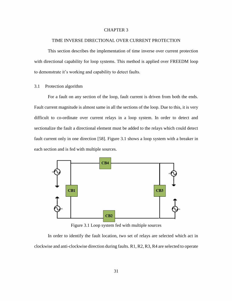
fault current only in one direction [58]. Figure 3.1 shows a loop system with a breaker in
each section and is fed with multiple sources.
Figure 3.1 Loop system fed with multiple sources
In order to identify the fault location, two set of relays are selected which act in
clockwise and anti-clockwise direction during faults. R1, R2, R3, R4 are selected to operate

32
in clockwise direction and R5, R6, R7, R8 in anti-clockwise direction. Figure 3.2 and
Figure 3.3 show the location of clockwise and anti-clockwise relays respectively.
Figure 3.2 Location of clockwise relays on the loop system
Figure 3.3 Location of anti-clockwise relays on the loop system
The location of a fault is sensed by the closest clockwise and anti-clockwise relays
located near the circuit breakers. In addition to the directional capability, relays are fed
with the time inverse over current characteristic. When a fault occurs, relays act according
to time inverse over current characteristics and the relays closest to the fault act first. For a
relay to respond, both the directional and time inverse over current element must be set at
high. The operation of relays during a fault is explained below in the Figure 3.4.
33
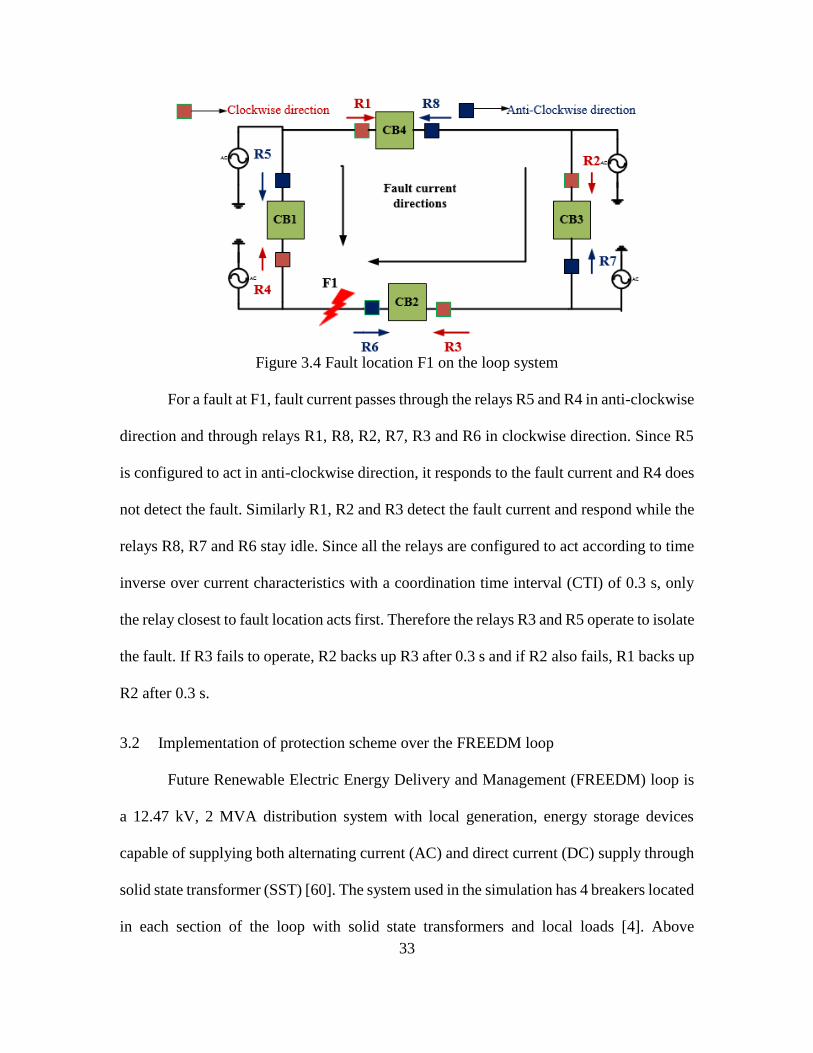
Figure 3.4 Fault location F1 on the loop system
For a fault at F1, fault current passes through the relays R5 and R4 in anti-clockwise
direction and through relays R1, R8, R2, R7, R3 and R6 in clockwise direction. Since R5
is configured to act in anti-clockwise direction, it responds to the fault current and R4 does
not detect the fault. Similarly R1, R2 and R3 detect the fault current and respond while the
relays R8, R7 and R6 stay idle. Since all the relays are configured to act according to time
inverse over current characteristics with a coordination time interval (CTI) of 0.3 s, only
the relay closest to fault location acts first. Therefore the relays R3 and R5 operate to isolate
the fault. If R3 fails to operate, R2 backs up R3 after 0.3 s and if R2 also fails, R1 backs up
R2 after 0.3 s.
3.2 Implementation of protection scheme over the FREEDM loop
Future Renewable Electric Energy Delivery and Management (FREEDM) loop is
a 12.47 kV, 2 MVA distribution system with local generation, energy storage devices
capable of supplying both alternating current (AC) and direct current (DC) supply through
solid state transformer (SST) [60]. The system used in the simulation has 4 breakers located
in each section of the loop with solid state transformers and local loads [4]. Above

34
mentioned algorithm is applied on the FREEDM loop and Figure 3.5 shows the model used
in simulation.
Figure 3.5 Arrangement of anti-clockwise relays on the FREEDM loop
In Figure 3.5, relays R1, R2 and R3 are anti-clockwise and RX is the sub-station
relay used to isolate the loop for faults near the sub-station. Co-ordination is done in such
a way that R2 backs up R1 and R3 backs up R2. If R3 fails, RX operates. Figure 3.6 shows
the arrangement of clockwise relays and their coordination.
Figure 3.6 Arrangement of clockwise relays on the FREEDM loop
Coordination is done such that R6 backs up R5, R5 backs up R4 and if R4 fails to
operate RX operates. Following section shows the operating relays and their corresponding

35
operating times for faults at various locations on the test bed at 0.2 s. For simulation, the
forward threshold impedance is taken to be 0.5 ohm and reverse threshold impedance is
taken to be 0.6 ohm. The area in between the CB1 and CB2 is considered as zone 1, CB2
and CB3 is considered as zone 2 and, CB3 and CB4 is considered as zone 3.
3.3 Single line to ground fault at location F1
Figure 3.7 shows the location of a single line to ground (SLG) fault F1 on phase A
at 0.2 seconds and the direction of fault currents in the loop. Calculations for current
transformer (CT) selection, current pick up values and time dial settings of the relay are
shown in the next section.
Figure 3.7 Fault current directions for fault at F1
For a fault F1 at 0.2 s, relays R1 and R6 act to isolate the fault. Relay R1 acts as the
fault current passes through it in anti-clockwise direction and R6 acts as fault current passes
through it in clockwise direction. Relays R4 and R5 also act as the fault current passes
through it in clockwise direction. But only the relays close to the fault acts first due to the

36
time inverse characteristics. R5 acts if R6 fails to operate with a co-ordination time interval
of 0.3 s. If R5 fails, R4 backs-up after 0.3 s.
Relays R1 and R6 are the primary relays. R1 operates at 0.293 s and R6 operates at
0.245 s. If R6 fails to operate, R5 backs up R6 with a CTI of 0.3 s at 0.545 s and if R5 fails,
R4 backs up R5 at 0.845 s. If all the relays fail to operate relay RX disconnects the supply
from the rest of the system. Time shown in the Figure 3.7 is the instance at which the relay
operates for fault at 0.2 s, not the time of operation. Time of operation of R1 is 0.293-
0.2=0.093 s which is approximately 5.8 cycles.
3.4 Single line to ground fault at location F2
Figure 3.8 shows the location of a single line to ground (SLG) fault F2 on phase
A at 0.2 seconds and the direction of fault currents in the loop.
Figure 3.8 Fault current directions for fault at F2
For a fault at F2, relays R2 and R5 are the primary relays. Relay R2 acts at 0.286 s
and R5 acts at 0.248 s. If R5 fails, R4 backs up R5 with a CTI of 0.3 s at 0.548 s. If R2

37
fails, R1 backs up R2 with CTI of 0.3 s at 0.586 s. If all the relays fail to act, then RX
disconnects the supply from the system.
3.5 Single line to ground fault at location at F3
Figure 3.9 shows the location of a single line to ground (SLG) fault F3 on phase A
at 0.2 seconds and the direction of fault currents in the loop.
Figure 3.9 Fault current directions for fault at F3
For a fault at F3, relays R4 and R3 are the primary relays. R3 acts at 0.248 s and
R4 acts at 0.276 s. If R3 fails to operate, R2 acts at 0.548 s and if R2 fails, R1 acts at 0.848
s. If R4 fails to operate, RX disconnects the supply from the system. Table 3.1 shows the
operation time of the relays for faults F1, F2 and F3 at 0.2 seconds.
Table 3.1 Operating times of relays corresponding to circuit breakers
Fault CB1 CB2 CB3 CB4
F1 0.093 s 0.045 s XXX XXX
F2 XXX 0.086 s 0.048 s XXX
F3 XXX XXX 0.048 s 0.076 s
38
3.6 Selection of time dial settings and current pick values for time inverse over current
relays
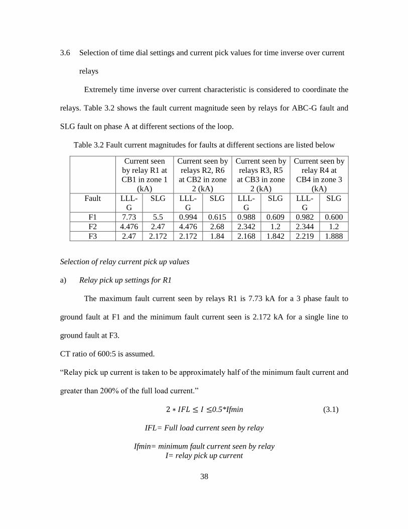
Extremely time inverse over current characteristic is considered to coordinate the
relays. Table 3.2 shows the fault current magnitude seen by relays for ABC-G fault and
SLG fault on phase A at different sections of the loop.
Table 3.2 Fault current magnitudes for faults at different sections are listed below
Current seen
by relay R1 at
CB1 in zone 1
(kA)
Current seen by
relays R2, R6
at CB2 in zone
2 (kA)
Current seen by
relays R3, R5
at CB3 in zone
2 (kA)
Current seen by
relay R4 at
CB4 in zone 3
(kA)
Fault LLL-
G
SLG LLL-
G
SLG LLL-
G
SLG LLL-
G
SLG
F1 7.73 5.5 0.994 0.615 0.988 0.609 0.982 0.600
F2 4.476 2.47 4.476 2.68 2.342 1.2 2.344 1.2
F3 2.47 2.172 2.172 1.84 2.168 1.842 2.219 1.888
Selection of relay current pick up values
a) Relay pick up settings for R1
The maximum fault current seen by relays R1 is 7.73 kA for a 3 phase fault to
ground fault at F1 and the minimum fault current seen is 2.172 kA for a single line to
ground fault at F3.
CT ratio of 600:5 is assumed.
“Relay pick up current is taken to be approximately half of the minimum fault current and
greater than 200% of the full load current.”
2 ∗ 𝐼𝐹𝐿 ≤ 𝐼 ≤0.5*Ifmin (3.1)
IFL= Full load current seen by relay
Ifmin= minimum fault current seen by relay
I= relay pick up current

39
2 ∗5 ∗ 20
600≤ 𝐼 ≤
0.5 ∗ 2172 ∗ 5
600
0.333 ≤ 𝐼 ≤ 9.05
𝐼 = 3 A is selected
b) Relay pick up settings for R2 and R6
The maximum fault current seen by R2 and R6 is 4.476 kA for a three phase to
ground fault at F2 and the minimum fault current seen is 615 A for a single line to ground
fault at F1.
CT ratio of 200:5 is assumed.
5 ∗ 2 ∗ 20
200≤ 𝐼 ≤
0.5 ∗ 5 ∗ 615
200
(3.2)
1 ≤ 𝐼 ≤ 7.68
𝐼 = 5
c) Relay pick up settings for R3 and R5
The maximum fault current seen by relays R3 and R5 is 2.342 kA for a 3 phase
fault to ground fault at F2 and the minimum fault current seen is 609 A for a single line to
ground fault at F1.
CT ratio of 200:5 is assumed.
5 ∗ 40 ∗ 2
200≤ 𝐼 ≤
0.5 ∗ 5 ∗ 609
200
2 ≤ 𝐼 ≤ 7.6125 (3.3)
𝐼 = 4

40
d) Relay pick up settings for R4
The maximum fault current seen by relays R4 is 2.344 kA for a 3 phase fault to
ground fault at F2 and the minimum fault current seen is 600 A for a single line to ground
fault at F1.
CT ratio of 200:5 is assumed.
5 ∗ 20 ∗ 2
200≤ 𝐼 ≤
0.5 ∗ 5 ∗ 600
200
1 ≤ 𝐼 ≤ 7.5 (3.4)
𝐼 = 7
The fault current magnitude near the relay RX would almost be equal to that of relay R4.
Hence a CT ratio of 200:5 is selected with a current pick up of 7 A.
Selection of time dial settings
In-order to determine time dial settings, maximum fault current seen by relays is
taken for calculation to ensure quick operation of relays for all type of faults. Table 3.3
shows the maximum current seen by the relays during fault conditions.
Table 3.3 Clockwise and anti- Clockwise relays
Relays in clockwise Relays in anti-clockwise
Relay acting as
primary
Relay acting as
back up
Relay acting as
primary
Relay acting as
back up
Fault Relay Current
seen
Relay Current
seen
Relay Current
seen
Relay Current
seen
F1 R6 994 A R5 998 A R1 7.73 kA RX 7.73
kA
F2 R5 2.342
kA
R4 2344 A R2 4.476
kA
R1 4.478
kA
F3 R4 2219 A RX 2220 A R3 2.168
kA
R2 2.170
kA

41
Time dial settings are determined from the co-ordination of relays. Coordination of relays
is explained in the following section.
Co-ordination of clockwise relays
i. Fault F1
For a fault at F1, R6 acts as primary protection and R5 acts as a back-up. Extremely
time inverse type over current relay is used. For the relay to act instantaneously time dial
settings for R6 is chosen to be 0.5, the minimum value for extremely inverse curve.
𝑇𝐷6 = 0.5
𝑡𝑟6 = 𝑇𝐷6 ∗ (0.0352 +5.67
𝑀2−1) (3.5)
𝑀 =𝐼𝑓𝑎𝑢𝑙𝑡 𝑠𝑒𝑒𝑛 𝑏𝑦 𝑅3
𝐼 𝑝𝑖𝑐𝑘 𝑢𝑝 =
𝐼𝑓𝑎𝑢𝑙𝑡 ∗ (1
𝐶𝑇 𝑟𝑎𝑡𝑖𝑜)
𝑟𝑒𝑙𝑎𝑦 𝑃𝑖𝑐𝑘 𝑢𝑝 𝑐𝑢𝑟𝑟𝑒𝑛𝑡
982 ∗ 5200⁄
5= 4.97
𝑡𝑟6 = 0.5 ∗ (0.0352 +5.67
4.912 − 1) = 0.13721 𝑠
Assuming a co-ordination time interval of 0.3 s, relay 5 operates at tr5= 0.13721+0.3 =
0.4372 s. Current seen by R5 for fault at F1 is 988 A.
𝑇𝐷5 =𝑡𝑟5
(0.0352 +5.67
𝑀2 − 1)
(3.6)
𝑀 =988 ∗ 5
200 ∗ 4= 6.175
𝑇𝐷5 = 2.326

42
ii. Fault F2
For a fault at F2, R5 acts as primary relay and R4 acts as back up relay. Time to
detect the fault current by relay R5 can be found by using the time dial setting of R5
calculated above step. Fault current seen by R5 is 2.342 kA.
𝑀 =2342 ∗ 5
200 ∗ 4= 14.637
(3.7)
𝑡𝑟5 = 2.326 ∗ (0.0352 +5.67
14.6372 − 1)
𝑡𝑟5 = 0.1437 𝑠
Relay R4 acts 0.3 s after the operation of R5. Time of operation of R4 is
0.1437+0.3=0.4437 s. Current seen by relay R4 for fault at F2 is 2.344 kA.
𝑀 =2344 ∗ 5
200 ∗ 7= 8.371
(3.8)
𝑇𝐷4 =𝑡𝑟4
(0.0352 +5.67
𝑀2 − 1)
= 3.78
Relay RX backs up R4 0.3 s after the operation of R4. tRX =0.4437+0.3= 0.7437 s. Current
sensed by the relay RX is 2219 A.
𝑀 =2219 ∗ 5
200 ∗ 7= 7.925
(3.9)
𝑇𝐷_𝑅𝑋 =𝑡𝑅𝑋
(0.0352 +5.67
𝑀2 − 1)
= 5.85

43
Co-ordination of anti-clockwise relays
i. Fault F3
For a fault at F3, R3 acts as primary relay and R2 acts as back up relay. Fault current
seen by R3 is 2.168 kA. For the relay to act instantaneously time dial settings for R3 is
chosen to be 0.5, the minimum value for extremely inverse curve.
𝑇𝐷3 = 0.5
𝑀 =2168 ∗ 5
200 ∗ 4= 13.55
(3.10)
𝑡𝑟3 = 𝑇𝐷3 ∗ (0.0352 +5.67
𝑀2 − 1) = 0.0331 𝑠
Relay R2 acts as back-up 0.3 seconds after the operation of R3. Time of operation of R2 is
tr2= 0.0331+0.3= 0.3331 s.
Time dial setting of R2 can be found out using the tr2 calculated in the above equation.
Fault current seen by R2 is 2170 A.
𝑀 =2170 ∗ 5
200 ∗ 5= 10.85
(3.11)
𝑇𝐷2 =𝑡𝑟2
(0.0352 +5.67
𝑀2 − 1)
= 3.9748
ii. Fault F2
For a fault at F2, R2 acts as primary relay and R1 acts as back up relay. Time to
detect the fault current by relay R2 can be found by using the time dial setting of R2
calculated in the above step. Fault current seen by R2 is 4.476 kA.
𝑀 =4476 ∗ 5
200 ∗ 5= 22.38
(3.12)
𝑡𝑟2 = 𝑇𝐷2 ∗ (0.0352 +5.67
𝑀2 − 1) = 0.1849 𝑠
44
Relay R1 acts as back up 0.3 seconds after the operation of R2. Time of operation
of R1 is tr1= 0.3+0.1849= 0.4849 s. Time dial settings of relay R1 can be found by using
tr1calculated in the above equation. Current seen by relay R1 is 4.478 kA.
𝑀 =4478 ∗ 5
600 ∗ 3= 12.43
(3.13)
𝑇𝐷1 =𝑡𝑟1
(0.0352 +5.67
𝑀2 − 1)
= 6.72
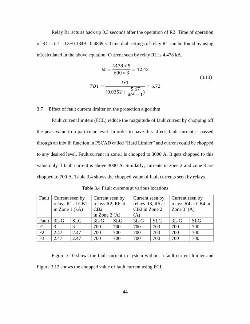
3.7 Effect of fault current limiter on the protection algorithm
Fault current limiters (FCL) reduce the magnitude of fault current by chopping off
the peak value to a particular level. In-order to have this affect, fault current is passed
through an inbuilt function in PSCAD called “Hard Limiter” and current could be chopped
to any desired level. Fault current in zone1 is chopped to 3000 A. It gets chopped to this
value only if fault current is above 3000 A. Similarly, currents in zone 2 and zone 3 are
chopped to 700 A. Table 3.4 shows the chopped value of fault currents seen by relays.
Table 3.4 Fault currents at various locations
Fault Current seen by
relays R1 at CB1
in Zone 1 (kA)
Current seen by
relays R2, R6 at
CB2
in Zone 2 (A)
Current seen by
relays R3, R5 at
CB3 in Zone 2
(A)
Current seen by
relays R4 at CB4 in
Zone 3 (A)
Fault 3L-G SLG 3L-G SLG 3L-G SLG 3L-G SLG
F1 3 3 700 700 700 700 700 700
F2 2.47 2.47 700 700 700 700 700 700
F3 2.47 2.47 700 700 700 700 700 700
Figure 3.10 shows the fault current in system without a fault current limiter and
Figure 3.12 shows the chopped value of fault current using FCL.

45
Figure 3.10 Fault current without current limiter
Figure 3.11 shows the hard limiter block in PSCAD and the implementation of
hard limiter. The input to the block must be an instantaneous value. Since the fault
current seen by relay has changed, the relay settings must be updated according to the
chopped value of fault current.
Figure 3.11 Implementation of fault current limiter in PSCAD
Figure 3.12 Fault current with current limiter

46
Selection of relay current pick up settings for chopped value of fault current
i. Relay pick up settings for R1
The maximum fault current seen by the relay R1 is 3 kA for a 3 phase fault to
ground fault at F1 and the minimum fault current seen is 2.47 kA for a single line to ground
fault.
CT ratio of 600:5 is assumed.
“Relay pick up current is taken to be approximately half of the minimum fault current
and greater than 200% of the full load current.”
2 ∗ 𝐼𝐹𝐿 ≤ 𝐼 ≤0.5*Ifmin
IFL= Full load current seen by relay
Ifmin= minimum fault current seen by relay
I= relay pick up current
2 ∗5 ∗ 20
600≤ 𝐼 ≤
0.5 ∗ 2470 ∗ 5
600
(3.14)
0.333 ≤ 𝐼 ≤ 10.29
𝐼 = 8 A is selected
ii. Relay pick up settings for R2 and R6
The maximum fault current seen by R2 and R6 is 700 A for a three phase to ground
fault at F2 and the minimum fault current seen is 700 A for a single line to ground fault at
F1.
CT ratio of 200:5 is assumed.
5 ∗ 2 ∗ 20
200≤ 𝐼 ≤
0.5 ∗ 5 ∗ 700
200
(3.15)
47
1 ≤ 𝐼 ≤ 8.75
𝐼 = 7 𝐴 𝑖𝑠 𝑠𝑙𝑒𝑐𝑡𝑒𝑑
iii. Relay pick up settings for R3 and R5
The maximum fault current seen by relays R3 and R5 is 700 A for a 3 phase fault
to ground fault at F3 and the minimum fault current seen is 700 A for a single line to ground
fault at F1.
CT ratio of 200:5 is assumed. 5 ∗ 40 ∗ 2
200≤ 𝐼 ≤
0.5 ∗ 5 ∗ 700
200
(3.16)
2 ≤ 𝐼 ≤ 8.75
𝐼 = 5 𝐴 𝑖𝑠 𝑠𝑒𝑙𝑒𝑐𝑡𝑒𝑑
iv. Relay pick up settings for R4
The maximum fault current seen by relays R4 is 700 A for a 3 phase fault to ground
fault at F3 and the minimum fault current seen is 700 A for a single line to ground fault at
F1.
CT ratio of 200:5 is assumed. 5 ∗ 20 ∗ 2
200≤ 𝐼 ≤
0.5 ∗ 5 ∗ 700
200
(3.17)
1 ≤ 𝐼 ≤ 8.75
𝐼 = 4.2 𝐴 𝑖𝑠 𝑠𝑒𝑙𝑒𝑐𝑡𝑒𝑑
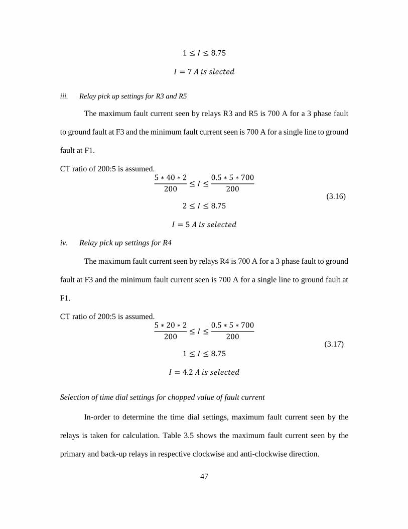
Selection of time dial settings for chopped value of fault current
In-order to determine the time dial settings, maximum fault current seen by the
relays is taken for calculation. Table 3.5 shows the maximum fault current seen by the
primary and back-up relays in respective clockwise and anti-clockwise direction.
48
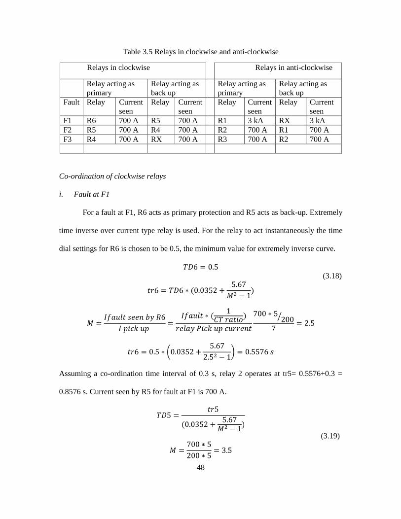
Table 3.5 Relays in clockwise and anti-clockwise
Relays in clockwise Relays in anti-clockwise
Relay acting as
primary
Relay acting as
back up
Relay acting as
primary
Relay acting as
back up
Fault Relay Current
seen
Relay Current
seen
Relay Current
seen
Relay Current
seen
F1 R6 700 A R5 700 A R1 3 kA RX 3 kA
F2 R5 700 A R4 700 A R2 700 A R1 700 A
F3 R4 700 A RX 700 A R3 700 A R2 700 A
Co-ordination of clockwise relays
i. Fault at F1
For a fault at F1, R6 acts as primary protection and R5 acts as back-up. Extremely
time inverse over current type relay is used. For the relay to act instantaneously the time
dial settings for R6 is chosen to be 0.5, the minimum value for extremely inverse curve.
𝑇𝐷6 = 0.5 (3.18)
𝑡𝑟6 = 𝑇𝐷6 ∗ (0.0352 +5.67
𝑀2 − 1)
𝑀 =𝐼𝑓𝑎𝑢𝑙𝑡 𝑠𝑒𝑒𝑛 𝑏𝑦 𝑅6
𝐼 𝑝𝑖𝑐𝑘 𝑢𝑝 =
𝐼𝑓𝑎𝑢𝑙𝑡 ∗ (1
𝐶𝑇 𝑟𝑎𝑡𝑖𝑜)
𝑟𝑒𝑙𝑎𝑦 𝑃𝑖𝑐𝑘 𝑢𝑝 𝑐𝑢𝑟𝑟𝑒𝑛𝑡
700 ∗ 5200⁄
7= 2.5
𝑡𝑟6 = 0.5 ∗ (0.0352 +5.67
2.52 − 1) = 0.5576 𝑠
Assuming a co-ordination time interval of 0.3 s, relay 2 operates at tr5= 0.5576+0.3 =
0.8576 s. Current seen by R5 for fault at F1 is 700 A.
𝑇𝐷5 =𝑡𝑟5
(0.0352 +5.67
𝑀2 − 1)
(3.19)
𝑀 =700 ∗ 5
200 ∗ 5= 3.5

49
𝑇𝐷5 = 1.5905
ii. Fault F2
For a fault at F2, R5 acts as primary relay and R4 acts as back up relay. Time to
detect the fault current by relay R5 can be found by using the time dial setting of R5
calculated above step. The fault current seen by R5 is 700 A.
𝑀 =700 ∗ 5
200 ∗ 5= 3.5
(3.20)
𝑡𝑟5 = 1.6 ∗ (0.0352 +5.67
4.1662 − 1)
𝑡𝑟5 = 0.8575 𝑠
Relay R4 acts 0.3 s after the operation of R5. Time of operation of R4 is
0.8575+0.3=1.1575 s. Current seen by relay R4 for fault at F2 is 700 A.
𝑀 =700 ∗ 5
200 ∗ 4.2= 4.166
(3.21)
𝑇𝐷4 =𝑡𝑟4
(0.0352 +5.67
𝑀2 − 1)
= 3.032
Relay RX acts 0.3 s after the operation of R4. Time of operation of RX is 1.1575+0.3=
1.4575 s. Current seen by RX for the fault F1 is 700 A.
𝑀 =700 ∗ 5
200 ∗ 4.2= 4.166
(3.22)
𝑇𝐷_𝑅𝑋 =1.4575
(0.0352 +5.67
𝑀2 − 1)
= 4.162

50
Co-ordination of anti-clockwise relays
i. Fault F3
For a fault at F3, R3 acts as primary relay and R2 acts as back up relay. Fault current
seen by R3 is 700 A. For the relay to act instantaneously, the time dial setting for R3 is
chosen to be 0.5, which is the minimum value for extremely time inverse curve.
𝑇𝐷3 = 0.5 (3.23)
𝑀 =700 ∗ 5
200 ∗ 5= 3.5
𝑡𝑟3 = 𝑇𝐷3 ∗ (0.0352 +5.67
𝑀2 − 1) = 0.2696 𝑠
Relay R2 acts as back up 0.3 seconds after the operation of R3. Time of operation of R2 is
0.2696+0.3=0.5696 s. The time dial setting of R2 can be found out using tr2 calculated in
the above equation. Fault current seen by R2 is 700 A.
𝑀 =700 ∗ 5
200 ∗ 7= 2.5
(3.24)
𝑇𝐷2 =𝑡𝑟6
(0.0352 +5.67
𝑀2 − 1)
= 0.52
ii. Fault F2
For a fault at F2, R2 acts as primary relay and R1 acts as back up relay. Time to
detect the fault current by relay R2 can be found by using the time dial setting of R2
calculated above. Fault current seen by R2 is 700 A.
𝑀 =700 ∗ 5
200 ∗ 7= 2.5
(3.25)
𝑡𝑟2 = 𝑇𝐷2 ∗ (0.0352 +5.67
𝑀2 − 1) = 0.58 𝑠

51
Relay R1 acts as back up relay 0.3 seconds after the operation of R2. Time of
operation of R1 is tr1= 0.3+0.58=0.879 s. The time dial setting of relay R1 can be found
by using tr1 calculated in the above equation. The current seen by relay R1 is 3kA.
𝑀 =2470 ∗ 5
600 ∗ 8= 3.12
(3.26)
𝑇𝐷1 =𝑡𝑟1
(0.0352 +5.67
𝑀2 − 1)
= 0.84169 = 0.85
3.8 Response time of the relays to detect and isolate the fault
Figure 3.13 shows the different protection zones and fault locations.
Figure 3.13 FREEDM Loop with different zones and fault locations
Fault F1
A single line to ground fault is applied on phase A near F1 at t=2 s, the time to clear
the fault and the fault current magnitude are shown below. Since F1 is located in zone 1,
the circuit breakers CB1 and CB2 operate to isolate the fault. Load current in zone 1 is 15
A (RMS) during the normal operation (obtained from the PSCAD file) and the fault current
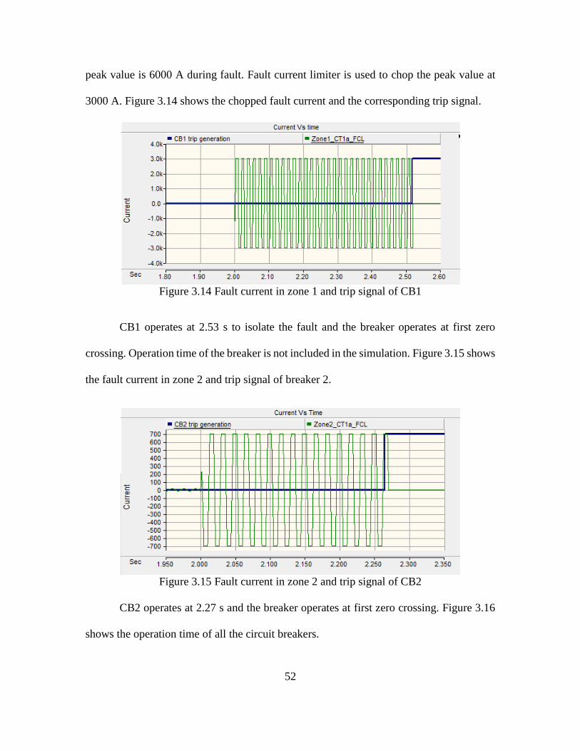
52
peak value is 6000 A during fault. Fault current limiter is used to chop the peak value at
3000 A. Figure 3.14 shows the chopped fault current and the corresponding trip signal.
Figure 3.14 Fault current in zone 1 and trip signal of CB1
CB1 operates at 2.53 s to isolate the fault and the breaker operates at first zero
crossing. Operation time of the breaker is not included in the simulation. Figure 3.15 shows
the fault current in zone 2 and trip signal of breaker 2.
Figure 3.15 Fault current in zone 2 and trip signal of CB2
CB2 operates at 2.27 s and the breaker operates at first zero crossing. Figure 3.16
shows the operation time of all the circuit breakers.

53
Figure 3.16 Operation time of circuit breakers for fault F1
The relays are coordinated such that they offer back-up protection when any of the
circuit breaker fails to operate. RX→R4→R5→R6 (Clockwise relays). Relay RX backs up
R4, R4 backs up R5 and R5 backs up R6 with a coordination time interval (CTI) of 0.3 s.
RX→R1→R2→R3 (Anti-Clockwise relays). Relay RX backs up R1, R1 backs up R2 and
R2 backs up R3 with a coordination time interval (CTI) of 0.3 s.
Back up protection when CB2 fails
Figure 3.17 shows the operation time of breakers CB3, CB4 and CB_X when the
breaker CB2 fails to operate. The time of operation of back up relays is found by disabling
the breaker operation for primary protection.
Figure 3.17 Operation time of back-up circuit breakers when CB2 fails to clear the fault
F1
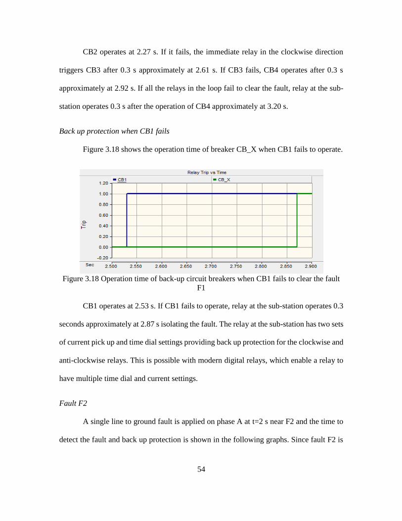
54
CB2 operates at 2.27 s. If it fails, the immediate relay in the clockwise direction
triggers CB3 after 0.3 s approximately at 2.61 s. If CB3 fails, CB4 operates after 0.3 s
approximately at 2.92 s. If all the relays in the loop fail to clear the fault, relay at the sub-
station operates 0.3 s after the operation of CB4 approximately at 3.20 s.
Back up protection when CB1 fails
Figure 3.18 shows the operation time of breaker CB_X when CB1 fails to operate.
Figure 3.18 Operation time of back-up circuit breakers when CB1 fails to clear the fault
F1
CB1 operates at 2.53 s. If CB1 fails to operate, relay at the sub-station operates 0.3
seconds approximately at 2.87 s isolating the fault. The relay at the sub-station has two sets
of current pick up and time dial settings providing back up protection for the clockwise and
anti-clockwise relays. This is possible with modern digital relays, which enable a relay to
have multiple time dial and current settings.
Fault F2
A single line to ground fault is applied on phase A at t=2 s near F2 and the time to
detect the fault and back up protection is shown in the following graphs. Since fault F2 is

55
located in zone 2, CB2 and CB3 act to isolate the fault. In this zone, the fault current is
chopped to 700 A. Figure 3.19 shows the current in zone 2 and trip signal of breaker 2.
Figure 3.19 Trip signal of CB2 for fault F2
CB2 operates at 2.23 s and the breaker operates at first zero crossing. Figure 3.20
shows current in zone 3 and trip signal of breaker 3.
Figure 3.20 Trip signal of CB3 for fault F2
CB3 operates at 2.47 s to isolate the fault and the fault current plummets to zero at
that instant. Figure 3.21 shows the operation time of all the circuit breakers.
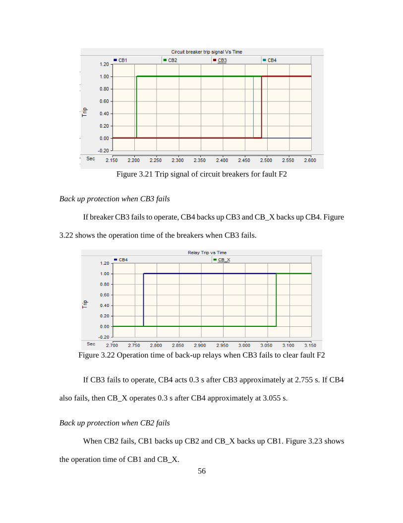
56
Figure 3.21 Trip signal of circuit breakers for fault F2
Back up protection when CB3 fails
If breaker CB3 fails to operate, CB4 backs up CB3 and CB_X backs up CB4. Figure
3.22 shows the operation time of the breakers when CB3 fails.
Figure 3.22 Operation time of back-up relays when CB3 fails to clear fault F2
If CB3 fails to operate, CB4 acts 0.3 s after CB3 approximately at 2.755 s. If CB4
also fails, then CB_X operates 0.3 s after CB4 approximately at 3.055 s.
Back up protection when CB2 fails
When CB2 fails, CB1 backs up CB2 and CB_X backs up CB1. Figure 3.23 shows
the operation time of CB1 and CB_X.

57
Figure 3.23 Operation time of back-up relays when CB2 fails to clear fault F2
When CB2 fails to clear the fault, CB1 operates after the CTI of 0.3 s approximately
at 2.5 s. If CB1 fails, then CBX operates 0.3 s after CB1 approximately at 2.8 s.
Fault F3
A single line to ground fault is applied on phase A at t=2 s and the corresponding
fault current is limited to 700 A. Figure 3.24 shows the operation of breaker 3 and fault
current in zone 2; Figure 3.25 shows the operation of breaker 4 and the fault current in zone
3.
Figure 3.24 Trip signal of CB3 for fault F3

58
Figure 3.25 Trip signal of CB4 for fault F3
Figure 3.26 shows the operation of the all primary circuit breakers. The circuit
breakers CB3 and CB4 operate at 2.291 s and 2.34 s respectively and the fault current
shoots down to zero as soon as the breakers operate.
Figure 3.26 Operation time of circuit breakers to isolate fault F3
Back-up protection when CB3 fails
Figure 3.27 shows the operation time of breakers CB2, CB1 and CB_X when CB
3 fails to clear the fault.
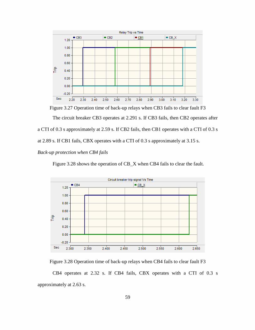
59
Figure 3.27 Operation time of back-up relays when CB3 fails to clear fault F3
The circuit breaker CB3 operates at 2.291 s. If CB3 fails, then CB2 operates after
a CTI of 0.3 s approximately at 2.59 s. If CB2 fails, then CB1 operates with a CTI of 0.3 s
at 2.89 s. If CB1 fails, CBX operates with a CTI of 0.3 s approximately at 3.15 s.
Back-up protection when CB4 fails
Figure 3.28 shows the operation of CB_X when CB4 fails to clear the fault.
Figure 3.28 Operation time of back-up relays when CB4 fails to clear fault F3
CB4 operates at 2.32 s. If CB4 fails, CBX operates with a CTI of 0.3 s
approximately at 2.63 s.

60
3.9 Variation of the trip signal for fault current chopped at different magnitudes
A SLG fault is applied at t=2 s at different locations of the loop and the trip
generation time is found out. Initially relays are coordinated to operate at their actual
values. Table 3.6, Table 3.7 and Table 3.8 show the response time of breakers for the fault
current chopped at different values.
Table 3.6 Fault currents chopped at 1/2 of their peak values
Fault CB1 CB2 CB3 CB4
F1 0.53 s 0.27 s XXX XXX
F2 XXX 0.21 s 0.47 s XXX
F3 XXX XXX 0.28 s 0.32 s
Table 3.7 Fault currents chopped at 1/3rd of their peak values
Fault CB1 CB2 CB3 CB4
F1 1.27 s 1.241 s XXX XXX
F2 XXX 1.119 s 1.51 s XXX
F3 XXX XXX 0.82 s 1.86 s
Table 3.8 Fault currents chopped at 1/6th of their peak values
Fault CB1 CB2 CB3 CB4
F1 2.823 s Failed to detect XXX XXX
F2 XXX Failed to detect 2.944 s XXX
F3 XXX XXX 2.584 s Failed to detect
To improve the operation time of relays, the time dial settings must be selected
according to the fault current limiting value.
3.10 Determining the directionality of fault current
The use of fault current direction simplifies the complexity involved in designing
the protection for loop systems. This method uses the negative sequence directional
element to determine the direction of fault current. “Negative sequence directional element
calculates the negative sequence impedance to determine the fault location. The calculated

61
scalar quantity 𝑍2 is compared with two threshold values to determine whether the fault is
in forward or reverse direction to a relay [59].
𝑍2 =𝑅𝑒[𝑉2.(𝐼2.1θ)∗]
𝑅𝑒[(𝐼2.1θ).(𝐼2.1θ)∗]=
𝑅𝑒[𝑉2.(𝐼2.1θ)∗]
𝐼22 (3.27)
𝑉2 = 𝑁𝑒𝑔𝑎𝑡𝑖𝑣𝑒 𝑠𝑒𝑞𝑢𝑒𝑛𝑐𝑒 𝑣𝑜𝑙𝑡𝑎𝑔𝑒
𝐼2 = 𝑁𝑒𝑔𝑎𝑡𝑖𝑣𝑒 𝑆𝑒𝑞𝑢𝑒𝑛𝑐𝑒 𝑐𝑢𝑟𝑟𝑒𝑛𝑡
𝑍2 = 𝑁𝑒𝑔𝑎𝑡𝑖𝑣𝑒 𝑆𝑒𝑞𝑢𝑒𝑛𝑐𝑒 𝐼𝑚𝑝𝑒𝑑𝑎𝑛𝑐𝑒
𝑖𝑓 𝑍2 < 𝑍2𝐹 , 𝑓𝑎𝑢𝑙𝑡 𝑖𝑠 𝑖𝑛 𝑓𝑜𝑟𝑤𝑎𝑟𝑑 𝑑𝑖𝑟𝑒𝑐𝑡𝑖𝑜𝑛
𝑖𝑓 𝑍2 > 𝑍2𝑅 , 𝑓𝑎𝑢𝑙𝑡 𝑖𝑠 𝑖𝑛 𝑟𝑒𝑣𝑒𝑟𝑠𝑒 𝑑𝑖𝑟𝑒𝑐𝑡𝑖𝑜𝑛
𝑖𝑓 𝑍2𝐹 < 𝑍2 < 𝑍2𝑅 , 𝑡ℎ𝑒𝑟𝑒 𝑖𝑠 𝑛𝑜 𝑓𝑎𝑢𝑙𝑡
𝑍2𝐹 = 𝐹𝑜𝑟𝑤𝑎𝑟𝑑 𝑡ℎ𝑟𝑒𝑠ℎ𝑜𝑙𝑑 𝑖𝑚𝑝𝑒𝑑𝑎𝑛𝑐𝑒
𝑍2𝑅 = 𝑅𝑒𝑣𝑒𝑟𝑠𝑒 𝑡ℎ𝑟𝑒𝑠ℎ𝑜𝑙𝑑 𝑖𝑚𝑝𝑒𝑑𝑎𝑛𝑐𝑒
During the normal operation, negative sequence quantities do not exist in the
system. The calculated negative sequence impedance lies within the forward threshold and
reverse threshold values. But during a faulted operation, sequential components come into
play and 𝑍2 could be used to determine the fault location. If the calculated 𝑍2 is less than
forward threshold impedance then the fault is in forward direction to a relay. If the
calculated 𝑍2 is greater than reverse threshold impedance then the fault is in reverse
direction to a relay. During a 3 phase to ground fault, negative sequence components are
negligible in the system and the directional element fails to detect the fault. To overcome
this particular scenario, relay uses positive sequence components during 3 phase faults to
detect directionality of the fault current.
3.11 Application of directionality in PSCAD
The sequence components of currents and voltages are obtained from the
fundamental phase quantities and are given as inputs to the ‘Negative sequence directional

62
element 32 Q’ available in PSCAD. The negative sequence directional element stays idle
during the normal operation and generates +1 or -1 depending on the fault location. It
behaves in the similar way as explained above. It uses negative sequences impedance as
the deciding factor to determine the fault location.
For a phase to ground fault, it uses the voltage of un-faulted phases for the relay to
be operational. Similarly, for a line-line fault, it uses the voltage of the un-faulted phases
to be operational. But for a 3phase-to-ground fault, the sequence components are less
dominant and it fails to detect the direction of fault. This hurdle can be overcomed when
digital relays are used. Digital relays (SEL 351S) invoke their internally stored memory
voltage during a three phase to ground fault. The protection scheme for a 3 phase fault is
validated on the real time digital simulator (RTDS) explained in the following section.
Figure 3.29 shows the implementation of directional element (32 Q element) in PSCAD.
Figure 3.29 Implementing directional element in PSCAD
Figure 3.32 shows the method to obtain sequence components required for the
operation of negative sequence directional element. It works in a similar way as explained
in the previous section. If the calculated 𝑍2 is less than forward threshold impedance 𝑍2𝐹,
the directional element generates +1 and if the calculated impedance is greater than the

63
reverse threshold impedance 𝑍2𝑅, it generates an output of -1. During normal operation it’s
output remains zero. Figure 3.30 and Figure 3.31 show the output of directional element
for faults in reverse and forward direction respectively.
Figure 3.30 Output of directional element for a reverse fault
Figure 3.31 Output of directional element for a forward fault
It can be seen in the figure 3.33 and figure 3.34, that the output of 32 Q element is
-1 for reverse fault, +1 for forward fault and it stays idle during normal operation.
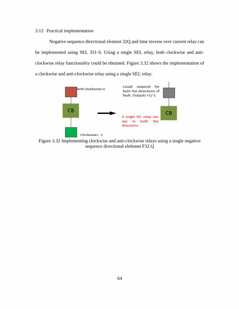
64
3.12 Practical implementation
Negative sequence directional element 32Q and time inverse over current relay can
be implemented using SEL 351-S. Using a single SEL relay, both clockwise and anti-
clockwise relay functionality could be obtained. Figure 3.32 shows the implementation of
a clockwise and anti-clockwise relay using a single SEL relay.
Figure 3.32 Implementing clockwise and anti-clockwise relays using a single negative
sequence directional elelemnt F32 Q

65
CHAPTER 4
PILOT DIRECTIONAL PROTECTION
Pilot directional protection uses the direction of fault current to determine the fault
location. A negative sequence directional element is used to determine the direction of fault
current (fault location). Working of negative sequence directional element is explained in
the previous section. Figure 4.1 shows the use of communication in determining the fault
location.
Figure 4.1 Radial system with sources fed from both ends
In Figure 4.1, fault current IF1 is sensed by the relays R1, R2 and fault current IF2
is sensed by the relay R3. R1, R2 and R3 calculate the negative sequence impedance
individually and compares with the threshold values to determine the fault location.
Directionality of the fault location is communicated between the relays R1, R2 and R2, R3.
If R1 and R2 have the same directionality, R1 does no generate the trip signal. If R2 and
R3 have different values of directionality, they generate the trip signals to breakers CB2
and CB3 to isolate the fault. Direction comparison is done only when current magnitude
crosses a threshold value and the voltage magnitude goes below a threshold value. This is
done to prevent any mis-trip which could occur due to the presence of negative sequence
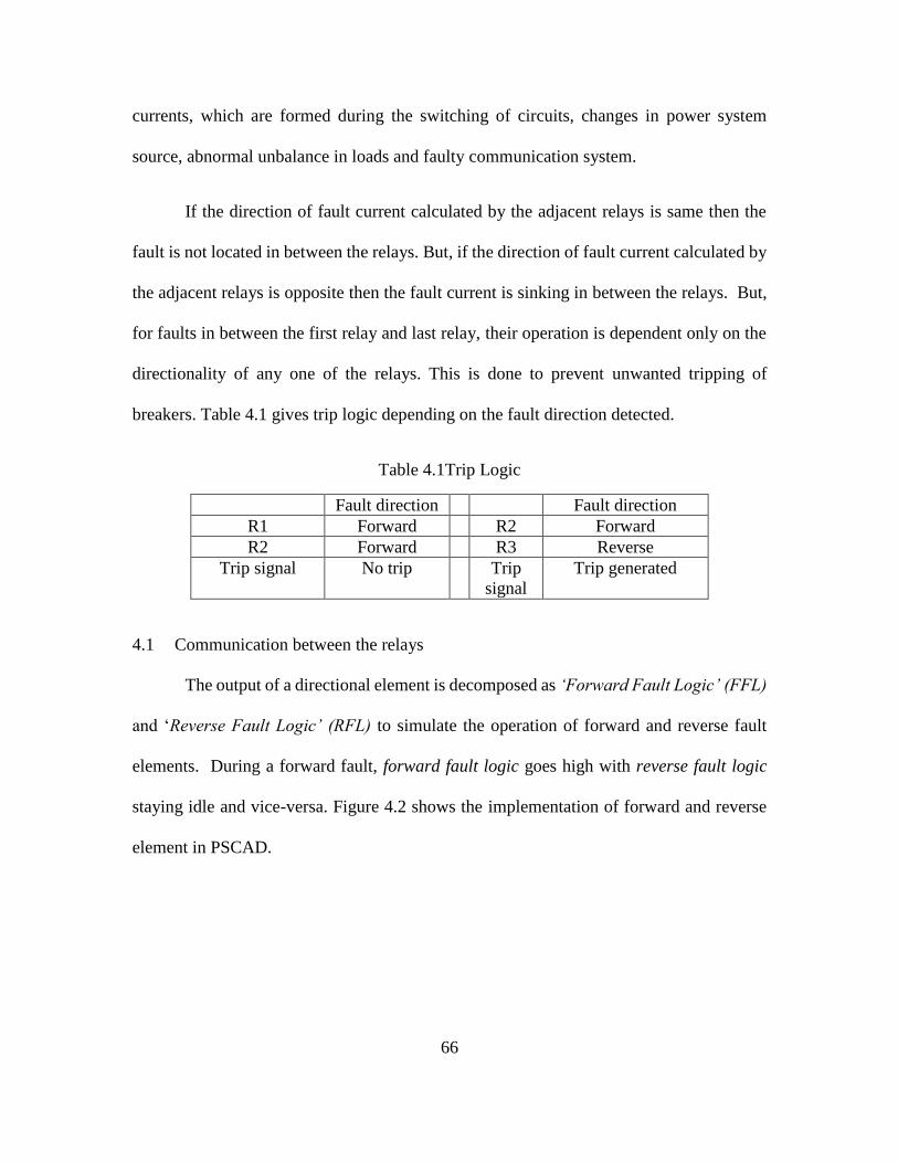
66
currents, which are formed during the switching of circuits, changes in power system
source, abnormal unbalance in loads and faulty communication system.
If the direction of fault current calculated by the adjacent relays is same then the
fault is not located in between the relays. But, if the direction of fault current calculated by
the adjacent relays is opposite then the fault current is sinking in between the relays. But,
for faults in between the first relay and last relay, their operation is dependent only on the
directionality of any one of the relays. This is done to prevent unwanted tripping of
breakers. Table 4.1 gives trip logic depending on the fault direction detected.
Table 4.1Trip Logic
Fault direction Fault direction
R1 Forward R2 Forward
R2 Forward R3 Reverse
Trip signal No trip Trip
signal
Trip generated
4.1 Communication between the relays
The output of a directional element is decomposed as ‘Forward Fault Logic’ (FFL)
and ‘Reverse Fault Logic’ (RFL) to simulate the operation of forward and reverse fault
elements. During a forward fault, forward fault logic goes high with reverse fault logic
staying idle and vice-versa. Figure 4.2 shows the implementation of forward and reverse
element in PSCAD.
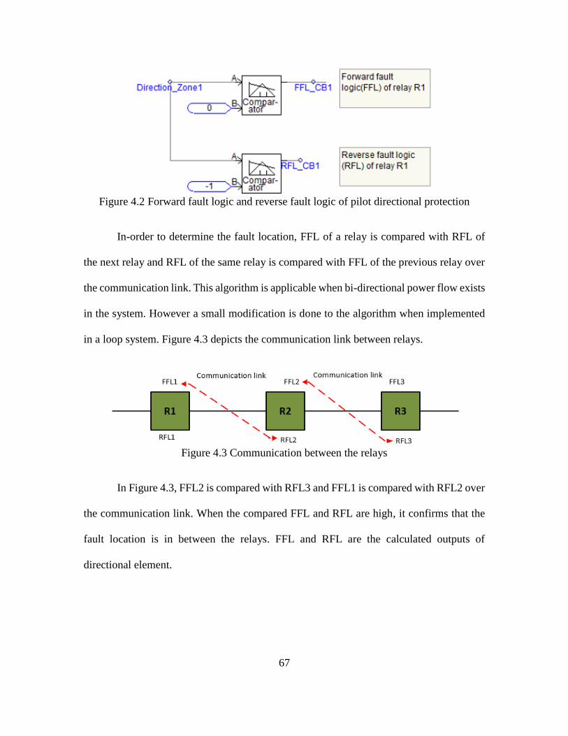
67
Figure 4.2 Forward fault logic and reverse fault logic of pilot directional protection
In-order to determine the fault location, FFL of a relay is compared with RFL of
the next relay and RFL of the same relay is compared with FFL of the previous relay over
the communication link. This algorithm is applicable when bi-directional power flow exists
in the system. However a small modification is done to the algorithm when implemented
in a loop system. Figure 4.3 depicts the communication link between relays.
Figure 4.3 Communication between the relays
In Figure 4.3, FFL2 is compared with RFL3 and FFL1 is compared with RFL2 over
the communication link. When the compared FFL and RFL are high, it confirms that the
fault location is in between the relays. FFL and RFL are the calculated outputs of
directional element.

68
4.2 Application of pilot directional scheme for the FREEDM system
PSCAD file of the FREEDM system used in the previous section is also used to
validate the pilot directional scheme. Figure 4.4 shows the FREEDM test bed used and the
fault locations F1, F2 and F3 in respective zones.
Figure 4.4 FREEDM loop with different zones and fault locations
Pilot directional algorithm is used as the protection scheme for the above loop
matching the hardware time delays (hardware is explained in the next section). Comparison
of directionality between CB1 and CB2, CB2 and CB3, CB3 and CB4 is done in the same
method as explained in the algorithm. But, the operation of CB1 and CB4 is coordinated
with the sub-station relay such that their operation is dependent up on the directional
element that goes high for faults in between CB1 and CB4. This ensures that they don’t
operate for a fault in any other section of the loop. This modification is done to prevent the
unwanted tripping of breakers in looped networks.

69
Average trip time for faults at various locations are shown below. Average trip time
is found by applying a fault in steps of 1 msec over 2 cycles and the average of the trip
signal time is taken. This is done using an inbuilt module in PSCAD. For simulation, the
forward threshold impedance is taken as 0.5 ohm and reverse threshold impedance is taken
as 0.6 ohm. Table 4.2 shows the operating time of breakers for different types of faults at
different locations.
Table 4.2 Trip signal delays for faults at different places
Fault
location
Fault
type
Breaker Avergae
delay
(msec)
F1 A-G CB1 18.25
F1 B-G CB1 18.25
F1 C-G CB1 18.21
F1 AB-G CB1 20.14
F1 BC-G CB1 19.82
F1 CA-G CB1 19.85
F1 A-B CB1 18.15
F1 B-C CB1 18.25
F1 C-A CB1 18.15
F2 A-G CB2 19.84
F2 B-G CB2 19.85
F2 C-G CB2 20.1
F2 AB-G CB2 22.13
F2 BC-G CB2 21.23
F2 CA-G CB2 22.56
F2 A-B CB2 21.5
F2 B-C CB2 23.6
F2 C-A CB2 22.3
F3 A-G CB3 21.84
F3 B-G CB3 21.84
F3 C-G CB3 21.83
F3 AB-G CB3 22.4
F3 BC-G CB3 23.84
F3 CA-G CB3 21.6
F3 A-B CB3 21.84
F3 B-C CB3 23.4
F3 C-A CB3 22.84
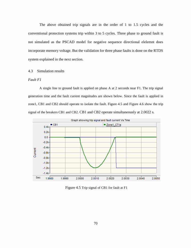
70
The above obtained trip signals are in the order of 1 to 1.5 cycles and the
conventional protection systems trip within 3 to 5 cycles. Three phase to ground fault is
not simulated as the PSCAD model for negative sequence directional elelemnt does
incorporate memory voltage. But the validation for three phase faults is done on the RTDS
system explained in the next section.
4.3 Simulation results
Fault F1
A single line to ground fault is applied on phase A at 2 seconds near F1. The trip signal
generation time and the fault current magnitudes are shown below. Since the fault is applied in
zone1, CB1 and CB2 should operate to isolate the fault. Figure 4.5 and Figure 4.6 show the trip
signal of the breakers CB1 and CB2. CB1 and CB2 operate simultaneously at 2.0022 s.
Figure 4.5 Trip signal of CB1 for fault at F1
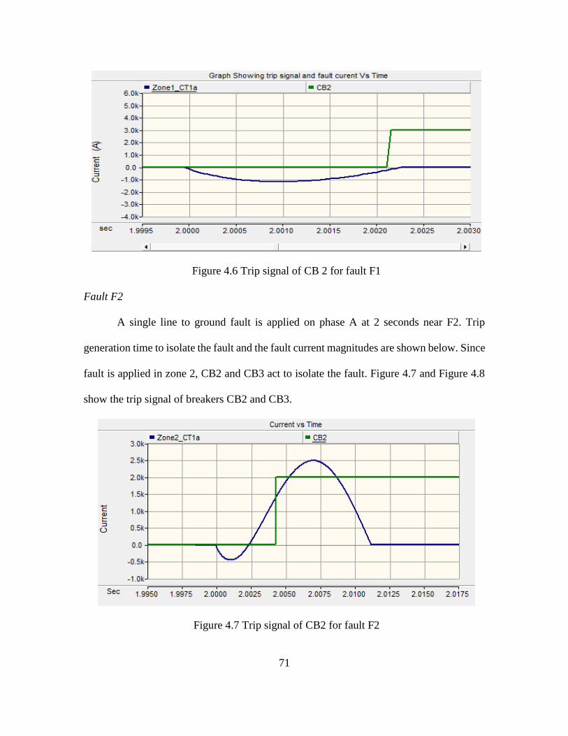
71
Figure 4.6 Trip signal of CB 2 for fault F1
Fault F2
A single line to ground fault is applied on phase A at 2 seconds near F2. Trip
generation time to isolate the fault and the fault current magnitudes are shown below. Since
fault is applied in zone 2, CB2 and CB3 act to isolate the fault. Figure 4.7 and Figure 4.8
show the trip signal of breakers CB2 and CB3.
Figure 4.7 Trip signal of CB2 for fault F2

72
Figure 4.8 Trip signal of CB3 for fault F2
The circuit breaker CB2 operates at 2.0041 s and CB3 operates at 2.002 s. Trip
signal to the circuit breaker CB2 is generated at 2.0041 s. Operation of the breaker takes
place at the next zero crossing of the current to clears the fault. The trip signal generated
in the simulation has a magnitude of 1. In-order to represent the decline of the fault current
against the trip signal the magnitude is scaled to 3000.
Fault F3
A single line to ground fault is applied on phase A near F3 at 2 seconds. Trip
generation time to isolate the fault and the fault current magnitudes are shown below. Since
the fault is applied in zone 3, CB3 and CB4 act to isolate the fault. Figure 4.9 and Figure
4.10 show the trip signal of CB3 and CB4. CB3 operates at 2.003 s and CB4 operates at
2.0023 s. All the circuit breakers operate at first zero crossing of the fault current.

73
Figure 4.9 Trip signal of CB3 for fault at F3
Figure 4.10 Trip signal of CB4 for fault at F3
Pilot protection scheme is very expensive when compared to the conventional
protection methods like over current and distance. But, pilot differential protection is
applied to few distribution feeders and transmission lines which carry significant amount
of power due to its fast clearing ability and robustness. The above described method can
be used for looped distribution networks with multiple sources as well as for the
transmission systems.

74
4.4 Hardware Implementation
Commercial Schweitzer relay SEL-351S is used to implement the pilot directional
algorithm. Figure 4.11 shows the single line diagram of a three phase test bed used for
hardware implementation.
Figure 4.11 Single line diagram of the hardware test bed
Hardware description
A 10 ohm resistor and 5 mH inductor connected in series is used to represent the
line impedance of a feeder with a load of 10 ohm resistor. A three phase 208 V 60Hz is
used as the power supply. A SLG fault is applied using ‘fault switch’ as shown in the above
picture with a fault resistor of 10 ohm. 100:5 CT’s are used to supply line currents to relays
R1 and R2. 1:1 isolation transformers are used as voltage inputs to both the relays. SEL-
2814 fiber-optic transceiver (serial to fiber interface) is used as a communication device
with fiber optic cable as the medium between the relays. Current in the test bed during

75
normal operation is 5 A but, when fault is created by turning ON the switch, current in
phase A jumps to 8 A.
Directional elements
R32Q and F32Q are the negative-sequence voltage polarized directional elements
used to determine fault current direction [5]. During the normal operation both the bits stay
low. But, during a forward fault to a relay F32Q goes high while R32Q stays idle and vice-
versa. Their operation is similar to the method as explained in the previous section. Relays
calculate the negative sequence impedance to determine the direction of fault current.
Mirrored bit communication and protection algorithm
Mirrored bit communication is the protocol used for communication between the
relays. Since the test bed used is a radial system, the fault current direction is from only
one end. Forward element of R1 (F32Q) is compared with forward element of R2 and
reverse element (R32Q) of R1 is compared with reverse element of R2 to determine the
fault current direction. The F32Q element of R1 is transmitted as a mirrored bit to R2 and
the F32Q of R2 is transmitted to R1. When both of them are high, fault is located at the
end of R2 and the relay is programmed to trip when it receives high signal from R1. Figure
4.12 depicts the communication method using mirrored bits [5] and [62].

76
Figure 4.12 Mirrored bit communication
Mirrored bits are transferred between the relays for every quarter cycle with a
sampling frequency of 128 Hz [61]. Figure 4.13 shows the hardware experimental setup.
Figure 4.13 Experimental set up for pilot directional protection
Figure 4.14 is generated using the SEL AcSELerator analytic assistant software. It
is used to view the trip signal generated against the system parameters.

77
Figure 4.14 Trip signal from acSELerator quikset software of SEL
Figure 4.18 depicts the change in frequency; increase in the magnitude of phase A
current and trip signal generation. The time delay between the instance of fault and trip
signal generation is found to be 1.094 cycle.
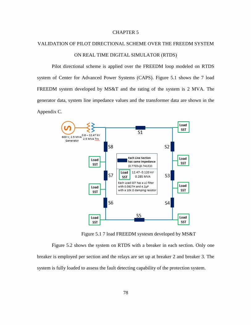
78
CHAPTER 5
VALIDATION OF PILOT DIRECTIONAL SCHEME OVER THE FREEDM SYSTEM
ON REAL TIME DIGITAL SIMULATOR (RTDS)
Pilot directional scheme is applied over the FREEDM loop modeled on RTDS
system of Center for Advanced Power Systems (CAPS). Figure 5.1 shows the 7 load
FREEDM system developed by MS&T and the rating of the system is 2 MVA. The
generator data, system line impedance values and the transformer data are shown in the
Appendix C.
Figure 5.1 7 load FREEDM systesm developed by MS&T
Figure 5.2 shows the system on RTDS with a breaker in each section. Only one
breaker is employed per section and the relays are set up at breaker 2 and breaker 3. The
system is fully loaded to assess the fault detecting capability of the protection system.

79
Figure 5.2 7 load FREEDM system modeled on RTDS
RTDS outputs the system voltage and currents in terms of voltage (AC or DC
depending on the system) with a maximum scale of 10 V. It’s output is interfaced to the
low voltage input of SEL 351 relay to measure to the system operating parameters. Relays
are connected at breaker 2 and breaker 3 locations. The fault location is chosen in between
breaker 2 and breaker 3 close to breaker 2 to simulate the worst case condition as the
voltage input to the relay plummets to zero during fault. Extensive study is done on trip
signal generation by applying 11 types of faults which includes single line to ground,
double line to ground, line to line, three phase to ground (ABC-G) and three phase line
faults (ABC-LLL) at 0 ° , 90 °, 180 °and 270 °. Following graphs show the fault current,
system voltage and the trip signal of breaker 2 and breaker 3. Relay settings are modified
according to the RTDS system parameters and operating conditions.

80
5.1 ABC to ground fault at zero degrees of phase A current
Figure 5.3 shows the trip signal of breaker 2 and the fault currents.
Figure 5.3 Trip signal of CB2 for 3 phase to ground fault
Time taken for the relay 2 to generate trip signal is 23.7 msec from the time of fault.
Figure 5.4 shows the system voltage near breaker 2 when the fault is cleared.
Figure 5.4 Voltage seen by relay during 3 phase fault
Figure 5.5 shows the trip signal of breaker 3.

81
Figure 5.5 Trip signal of CB3 for 3 phase to ground fault
Time taken for the relay 3 to generate trip signal is 25.8 msec from the time of fault.
The above graphs show the validation of the protection scheme an ABC to ground fault.
The basic foundation of the protection algorithm is to detect the fault location
(directionality property) using the negative sequence impedance. Negative sequence and
zero sequence components are negligible (very less) during a 3 phase to ground fault and
only positive sequence currents flow in the system. In addition to this, the entire voltage of
the loop momentarily goes to zero during a three phase fault (bolted ground fault) and the
relay has no input voltage to operate. Relay uses memory voltage to detect three phase
faults. Memory voltage is the momentary voltage which the relay stores before the voltage
of all phases goes to zero. Relay uses this memory voltage and positive sequence
components (F 32P element) to determine the fault location.
Figure 5.6 shows the phase currents, phase voltages, sequence components during
fault in the system. It can be seen that the negative sequence current and zero sequence
currents are very less when compared to positive sequence currents in the system. Relay
uses the positive sequence current and memory voltage to determine the direction.

82
Figure 5.6 File generated from acSELerator quickset for 3 phase fault
5.2 ABC-LLL fault at zero degree of phase A current
Figure 5.7 shows the trip signal of breaker 2 and fault current.
Figure 5.7 Trip signal of CB2 for ABC-LLL fault
Time taken by relay 2 to generate trip signal is 26.4 msec. Figure 5.8 shows the
system voltage near breaker 2 during fault and Figure 5.9 shows trip signal of breaker 3.

83
Figure 5.8 Voltage seen by relay for ABC-LLL fault
Figure 5.9 shows trip signal of breaker 3 and fault current.
Figure 5.9 Trip signal of CB3 for ABC-LLL fault
Time taken by relay 3 to generate trip signal is 26.2 msec. Graphs for the rest of the
fault types and fault angles are shown in the appendix A. Table 5.1 and Table 5.2 show the
trip time for all faults at different fault angles for breaker 2 and breaker 3.

84
Table 5.1 BRK 2 trip times for different fault angles
Fault type 0 degree 90 degree 180 degree 270 degree
SLG-A 23.7 msec 22.2 msec 26.8 msec 26.5 msec
SLG-B 20 msec 23.3 msec 26.8 msec 21.7 msec
SLG-C 31.4 msec 25.7 msec 27.9 msec 28.2 msec
ABC-G 23.78 msec 23.4 msec 23.8 msec 24.7 msec
AB (LL) 25.5 msec 20.4 msec 24 msec 27.2 msec
BC (LL) 25.9 msec 26.1 msec 25.5 msec 31.1 msec
CA (LL) 26.9 msec 28.4 msec 31.5 msec 20.5 msec
AB-G 24.9 msec 20 msec 25.6 msec 25.3 msec
BC-G 21.1 msec 29.8 msec 23.1 msec 33.5 msec
CA-G 24.2 msec 29.2 msec 27.6 msec 25.9 msec
ABC-LLL 26.4 msec 20.2 msec 19.6 msec 23.4 msec
Table 5.2 BRK 3 trip times for different fault angles
Fault Type 0 degrees 90 degrees 180 degrees 270 degrees
SLG A 40.1 msec 36.7 msec 28.4 msec 27.8 msec
SLG B 28.3 msec 35.1 msec 39.3 msec 41 msec
SLG C 35.8 msec 59.2 msec 27.4 msec 28.2 msec
ABC-G 25.8 msec 23 msec 24.8 msec 38.3 msec
AB (LL) 26.4 msec 29.9 msec 36.9 msec 35.3 msec
BC (LL) 45.36 msec 37.3 msec 42.1 msec 26.6 msec
CA (LL) 35.7 msec 37.3 msec 39.8 msec 36.19 msec
AB-G 20.1 msec 31.8 msec 32.9 msec 23 msec
BC-G 27.2 msec 56.9 msec 20.2 msec 55.4 msec
CA-G 42.2 msec 38.2 msec 41 msec 30.9 msec
ABC-LLL 26.2 msec 27.2 msec 22.5 msec 35.4 msec
Time taken by the relays to detect fault is in between 1.25 to 2.37 cycles. These
results are obtained from the 7 load RTDS FREEDM model when actual relays are used.
This is the only protection model that has been validated for the complete FREEDM loop
unlike the pilot differential protection which has been validated on a simple radial system.

85
CHAPTER 6
PMU BASED PROTECTION
Voltage phase angles are the primary variables that get affected during an event in
power system. Effective monitoring of these variables could help the power system
operators to respond quickly during unexpected contingencies. In this method the variation
of voltage phase angle during a fault is used as a deciding factor to trip the breakers. The
voltage phase angle difference between the ends of a transmission line is compared to a
predefined value and the comparison is done only when the current magnitude is higher
than 120 % of full load current and voltage magnitude is below 80 % of the rated value.
The predefined value is the voltage phase angle difference between the ends of a
transmission line during maximum power flow. The calculations for pre-set values are
shown in the appendix D.
A PMU is installed in every section of the loop to monitor the synchrophasor data.
Typically PMU’s are available in the modern digital relays and can be used to record the
synchrophasors. No additional device is added to monitor the synchrophasors, but the PMU
in the relay is enabled. Figure 6.1 shows location of PMU installed on the FREEDM loop
system. The absolute value of phase angle difference during maximum allowable power
flow between PMU1 and PMU 2 is 14.74 degrees, between PMU 2 and PMU 3 is 7.63
degrees, between PMU 3 and PMU 4 is 16.8261 degree, between PMU 4 and PMU 1 is
9.7484 degrees.

86
Figure 6.1 FREEDM system showing PMU location
6.1 Single line to ground fault on phase A near F1 at 2 seconds
Figure 6.2 Logic to detect an event using synchrophasor measurements
Figure 6.2 shows the algorithm using voltage phase angle data to detect faults.
Normal operating current in the loop is around 15 A and the current in the system is
compared to 120 % of the nominal current (approximately 20 A). The nominal phase

87
voltage of the system is 7.19 kV and voltage magnitude of a phase is compared to 6400 V
(around 85 % of the actual value). During a fault, the voltage of the system goes below the
operating value and the current magnitude shoots higher than the normal current. The
above must be met to guarantee the existence of fault in the system. The voltage phase
angle difference of phase A between PMU 1 and PMU 2 is compared to a predefined value
20 degrees (determined from the voltage phase angle difference during maximum power
flow). During any event, the phase angle difference fluctuates and finally settles to a new
value. The output of the voltage comparator, current magnitude comparator and voltage
phase angle difference comparator is given to an AND logic. Following graphs show the
variation of voltage phase angle difference between PMU 1 and PMU 2, PMU 2 and PMU
3, PMU 3 and PMU 4, PMU 4 and PMU 1.
Figure 6.3 Voltage phase difference of phase A between PMU 1 and PMU 2 for a SLG
fault
In Figure 6.3 it can be seen that for a fault at 2 seconds, the voltage phase angle
difference deviates from its initial value and settles at around -30 degrees. The absolute
value of voltage phase angle difference is compared to the threshold value to determine the

88
fault condition. Figure 6.4 shows the absolute value of voltage phase angle difference of
phase A between PMU 1 and PMU 2.
Figure 6.4 Absolute value of voltage phase differene of phase A between PMU 1 and
PMU 2 for a SLG fault
The time taken to generate the trip signal is around 15.5 msec and it does not include
the communication delay to transfer the phase angle information between the relays. Figure
6.5 shows the variation of voltage phase angle difference of phase A between PMU 2 and
PMU 3.
Figure 6.5 Voltage phase difference of phase A between PMU 2 and PMU 3 for a SLG
fault

89
Figure 6.6 and Figure 6.7 show the variation of voltage phase angle difference of phase A
between PMU 3 and PMU 4, PMU 4 and PMU 1.
Figure 6.6 Voltage phase difference of phase A between PMU 3 and PMU 4 for a SLG
fault
Figure 6.7 Voltage phase difference of phase A between PMU 4 and PMU 1 for a SLG
fault
In Figure 6.5, Figure 6.6 and Figure 6.7 it can be seen that the variation of phase
angle difference between PMU’s is not more than 6 degrees during fault which is less than
the phase difference during maximum allowable power flow. This ensures that other

90
breakers are not operated other than breaker 1 and breaker 2 for a fault at F1. Figure 6.8
shows the decrease of current in zone 1 when fault F1 is cleared by breakers.
Figure 6.8 Decrese in fault current due to the isolation of fault
6.2 3 phase to ground fault near F1 at 2 seconds
Figure 6.9 shows the variation of voltage phase angle difference of phase A
between PMU1 and PMU 2 for a 3 phase to ground fault at F1. The phase difference settles
to 30 degrees during fault condition.
Figure 6.9 Voltage phase difference of phase A between PMU 1 and PMU 2 for ABC-G
fault

91
Figure 6.10 shows the variation of voltage phase of phase B between PMU 1 and
PMU 2 for a 3 phase to ground fault. The voltage phase angle undergoes a huge transition
and settles at 300 degrees.
Figure 6.10 Voltage phase difference of phase B between PMU 1 and PMU 2 for ABC-G
fault
Figure 6.11 shows the voltage phase angle difference of phase C between PMU 1
and PMU 2. The phase difference settles to 40 degrees during fault.
Figure 6.11 Voltage phase difference of phase C between PMU 1 and PMU 2 for ABC-G
fault

92
Figure 6.12 shows the trip signal generation using the same algorithm used for
single line to ground faults. The logic to detect 3 phase to ground fault is same as to
detecting a single line to ground fault as the variation of phase angle difference of phase A
is similar.
Figure 6.12 Trip signal generated from PMU 1 and PMU 2 data
Figure 6.13, Figure 6.14 and Figure 6.15 shows the variation of voltage phase angle
difference of phase A between PMU’s in healthy part of the system.
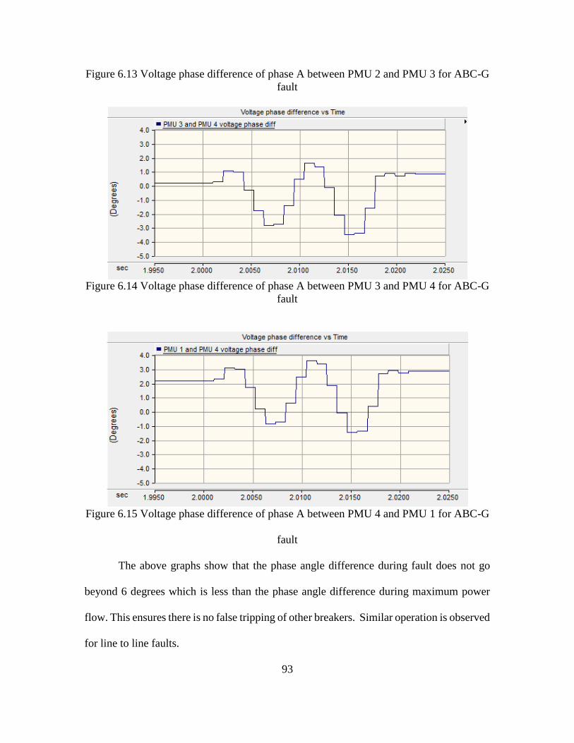
93
Figure 6.13 Voltage phase difference of phase A between PMU 2 and PMU 3 for ABC-G
fault
Figure 6.14 Voltage phase difference of phase A between PMU 3 and PMU 4 for ABC-G
fault
Figure 6.15 Voltage phase difference of phase A between PMU 4 and PMU 1 for ABC-G
fault
The above graphs show that the phase angle difference during fault does not go
beyond 6 degrees which is less than the phase angle difference during maximum power
flow. This ensures there is no false tripping of other breakers. Similar operation is observed
for line to line faults.

94
Power electronic converters impact the voltage magnitude, current magnitude and
voltage phase angle to facilitate bi-directional power flow in the loop. During faults the
substation SST in the loop voluntarily reduces the system voltage to limit the fault current
to 2 per unit. Substation SST controls only the voltage magnitude and current magnitude
but does not influence the voltage phase angle during a fault. Due to this peculiar operation
PMU based protection is highly reliable where other protection schemes fail to detect faults
(assuming no failure in communication channel).
6.3 Hardware implementation
A three phase test bed is used to implement the above algorithm and generate the
trip signal based on the variation of the voltage phase angle difference. Two 351S relays
are used to collect the synchrophasor data from the ends of test bed. The synchrophasor
data obtained is time stamped with a satellite enabled GPS clock SEL 2407 (IRIG-B
signal). The collected synchrophasor data is passed onto the synchro-vector processor SEL
3378 (SVP) which is used to analyze the synchrophasor data. The voltage phase angle
information is passed to adjacent SEL 3378 via fiber-optic cable using mirrored bit
communication. Thus the phase angle information is passed from one PMU to the other
PMU which is used for processing. The relays and synchro-vector processor is
programmed in such a way that it computes the voltage phase angle comparison only when
the voltage magnitude and current magnitude criteria met.
Inorder to collect, read and process the synchrophasor data SEL 5073, PDC
assistant, SVP Configurator and synchrowave central software are required to run
simultaneously on the computer. Relays collect the PMU data from the system but they
require SEL 5073 software to read the data from the relays onto the synchro vector

95
processor (SVP). SVP configurator helps in processing and analyzing the data while PDC
assistant along with Synchrowave central software helps to view the synchrowave data. All
these software are required to run simultaneously to view the real time data. Figure 6.16
shows the block diagram presentation of implementing hardware.
Figure 6.16 Hardware set up for PMU based protection
Relays SEL 351 collects the PMU data from network 1 and network 2. The data is
sent into the SEL 3378 (SVP-synchro vector processor) using the ethernet cable. PMU data
is transferred between the 3378’s via the fiber optic cable using the mirrored bit
communication. Once the data processor (SEL 3378) receives the PMU data, it calculates
the voltage phase angle difference between the two nodes, if the voltage magnitude goes
below a threshold value and the current magnitude goes above a threshold value and sends
a trip command to the relays. Program used in SVP configurator to communicate with
synchro vector processor is shown in appendix B. Figure 6.17 shows the single line
diagram of a 3 phase test bed on which testing is carried out.

96
Figure 6.17 Single line diagram of 3 phase test bed used in hardware implementation
Fault is applied in between 10 ohm and 5 mH reactor and the voltage phase between
the relay locations are monitored in the same way as explained above. Figure 6.18 shows
the variation of voltage phase from steady state condition of 141 degrees to 25 degrees.
Even though the network is a simple radial system with a 3 phase source, the hardware
implementation is done to make sure that the voltage phase angles vary as expected in the
simulation. A real time testing has to be done on the RTDS system to understand the
complete behavior of voltage phase angles during an event.
Figure 6.18 Graph obtained from the sychro vector processor

97
CHAPTER 7
CONCLUSIONS AND FUTURE WORK
7.1 Conclusions
This research work was aimed at developing protection schemes that could solve
the problem of communication in pilot differential protection developed by previous
FREEDM students at ASU. Due to the presence of distribution type solid state transformers
(SST) the power flow in the system is bi-directional and convention protection schemes
cannot be used. The substation SST reduces the voltage of system during faults to limit the
fault current to 2 per unit. Because of the reduced fault current magnitude, fast tripping
scheme could be compromised. However it is not advisable to allow a fault to persistent
for a longer duration as it will effect the power supply to healthy parts of system.
Considering all the operating conditions, three protection schemes have been developed.
Following are the various conclusions drawn from this research work.
Time inverse directional over-current (TIDOC) protection is developed using
directionality and time inverse characteristics with proper coordination of relays in the
looped system.
TIDOC protection could be used as a reliable back-up scheme when the communication
system fails, as it does not require communication channel to detect and sectionalize
the fault in a loop system with multiple sources.
TIDOC protection has inherent back-up protection when the primary breakers fail to
clear the fault. Table 7.1, 7.2 and 7.3 show the operation time of relays for faults at
various locations and when fault current is chopped at different levels. Relay settings
used for the simulation correspond to the actual fault current.
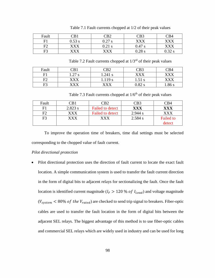
98
Table 7.1 Fault currents chopped at 1/2 of their peak values
Fault CB1 CB2 CB3 CB4
F1 0.53 s 0.27 s XXX XXX
F2 XXX 0.21 s 0.47 s XXX
F3 XXX XXX 0.28 s 0.32 s
Table 7.2 Fault currents chopped at 1/3rd of their peak values
Fault CB1 CB2 CB3 CB4
F1 1.27 s 1.241 s XXX XXX
F2 XXX 1.119 s 1.51 s XXX
F3 XXX XXX 0.82 s 1.86 s
Table 7.3 Fault currents chopped at 1/6th of their peak values
Fault CB1 CB2 CB3 CB4
F1 2.823 s Failed to detect XXX XXX
F2 XXX Failed to detect 2.944 s XXX
F3 XXX XXX 2.584 s Failed to
detect
To improve the operation time of breakers, time dial settings must be selected
corresponding to the chopped value of fault current.
Pilot directional protection
Pilot directional protection uses the direction of fault current to locate the exact fault
location. A simple communication system is used to transfer the fault current direction
in the form of digital bits to adjacent relays for sectionalizing the fault. Once the fault
location is identified current magnitude (𝐼𝐹 > 120 % 𝑜𝑓 𝐼𝐿𝑜𝑎𝑑) and voltage magnitude
(𝑉𝑠𝑦𝑠𝑡𝑒𝑚 < 80% 𝑜𝑓 𝑡ℎ𝑒 𝑉𝑟𝑎𝑡𝑒𝑑) are checked to send trip signal to breakers. Fiber-optic
cables are used to transfer the fault location in the form of digital bits between the
adjacent SEL relays. The biggest advantage of this method is to use fiber-optic cables
and commercial SEL relays which are widely used in industry and can be used for long

99
distances with little latency. Pilot directional method can be used to protect any looped
systems with multiple sources.
Pilot differential protection requires time stamped current signals (magnitude and phase
angle) at every load point. The communication channel should be fast with minimum
delay and the data analyzing capability should be very high to accurately detect the
fault and make sure the trip is not generated during normal operation. But the pilot
directional protection requires the transfer of only the fault location in the form of
digital bits to adjacent relays. It does not require a processing unit to collect the data,
process and send the trip to appropriate breakers in the faulted zone. The algorithm
inherently has fault sectionalizing capability with the communication of fault location.
Pilot directional algorithm should be modified to use for radial systems. However, it is
advisable to use conventional schemes (over-current) to protect radial systems which
is economical over pilot schemes. Table 7.4 and Table 7.5 show the operation time of
relays when validated on the RTDS system. 11 different types of faults are applied on
all phases at 0 degrees, 90 degrees, 180 degrees, 270 degrees and their trip time are
shown in the following table.
Table 7.4 Breaker 2 trip time for different fault angles
Fault type 0 degree 90 degree 180 degree 270 degree
SLG-A 23.7 msec 22.2 msec 26.8 msec 26.5 msec
SLG-B 20 msec 23.3 msec 26.8 msec 21.7 msec
SLG-C 31.4 msec 25.7 msec 27.9 msec 28.2 msec
ABC-G 23.78 msec 23.4 msec 23.8 msec 24.7 msec
AB (LL) 25.5 msec 20.4 msec 24 msec 27.2 msec
BC (LL) 25.9 msec 26.1 msec 25.5 msec 31.1 msec
CA (LL) 26.9 msec 28.4 msec 31.5 msec 20.5 msec
AB-G 24.9 msec 20 msec 25.6 msec 25.3 msec
BC-G 21.1 msec 29.8 msec 23.1 msec 33.5 msec
CA-G 24.2 msec 29.2 msec 27.6 msec 25.9 msec

100
ABC-LLL 26.4 msec 20.2 msec 19.6 msec 23.4 msec
Table 7.5 Breaker 3 trip time for different fault angles
Fault Type 0 degrees 90 degrees 180 degrees 270 degrees
SLG A 40.1 msec 36.7 msec 28.4 msec 27.8 msec
SLG B 28.3 msec 35.1 msec 39.3 msec 41 msec
SLG C 35.8 msec 59.2 msec 27.4 msec 28.2 msec
ABC-G 25.8 msec 23 msec 24.8 msec 38.3 msec
AB (LL) 26.4 msec 29.9 msec 36.9 msec 35.3 msec
BC (LL) 45.36 msec 37.3 msec 42.1 msec 26.6 msec
CA (LL) 35.7 msec 37.3 msec 39.8 msec 36.19 msec
AB-G 20.1 msec 31.8 msec 32.9 msec 23 msec
BC-G 27.2 msec 56.9 msec 20.2 msec 55.4 msec
CA-G 42.2 msec 38.2 msec 41 msec 30.9 msec
ABC-LLL 26.2 msec 27.2 msec 22.5 msec 35.4 msec
Protection, monitoring and control using synchrophasor data
During a fault in the system substation SST controls voltage magnitude to control fault
current magnitude. Voltage phase angle is left unaltered during fault conditions.
Monitoring voltage phase angle could be a reliable way to detect events (faults) in the
system.
During the normal operation, phase difference between two buses is almost zero or a
low value. But during a fault it undergoes a transition and settles to a higher value than
the phase difference during maximum power flow (𝛿𝑉𝑚𝑎𝑥) through the line. This
variation of voltage phase angle difference during fault is compared with 𝛿𝑉𝑚𝑎𝑥 to
detect fault. Comparison is done only when voltage goes below a certain value and
current goes above a certain value.

101
The transient change or oscillation of voltage phase angle difference of the unfaulted
section is below the 𝛿𝑉𝑚𝑎𝑥. This ensures that the breakers in the un-faulted section do
not operate.
PSCAD simulation for the PMU based protection is done and the time to detect the
occurrence of an event is found to be 15.5 msec.
Pilot differential protection and synchrophasor based protection do not have back up
protection like TIDOC protection.
TIDOC and pilot directional can be used for only 3 phase systems due to the presence
of negative sequence directional element. PMU based protection can be used for both
3 phase and single phase systems.
7.2 Things to take care when implementing above mentioned schemes
Directional element
Negative sequence directional element is used to find the direction of fault current. It has
several parameters like forward threshold impedance, reverse threshold impedance,
forward over current setting, reverse over current setting, positive sequence restraining
factor, zero-sequence restraining factor which should be set properly considering the line
impedance. In addition the direction of power flow should also be considered while
selecting the threshold impedance (forward and reverse) parameters. If the direction of
power flow is reverse then the positive threshold impedance values cannot detect the
direction, while negative threshold values of the same magnitude can be detected. If the
polarity of current transformer (CT) to the relay is reversed then the directionality may give
opposite results. Positive sequence directional element (F32P) must be set to ensure the
operation of relay for 3 phase faults (this is specific to SEL relays). When working on the

102
RTDS system CT ratio setting of the relay must never be set to 1 even though the CT ratio
factor is included within the RTDS software at the output terminals. If it is set to 1 then
F32P element goes high even during normal operation and might end up calculating the
settings which may be larger than the highest limits of the relay.
Selection of time dial settings for time inverse over current relay
Every relay has two sets of time dial and current pick up settings allowing the relay
to operate in both the directions (clockwise and anti-clockwise assuming the system is a
looped network like FREEDM system). As the number of breakers in the loop increase the
time dial and current pick up settings gets doubled. For adjacent relays, care must be taken
to properly select the time dial settings without which the time current characteristics are
going to get over-lapped and may result in unwanted tripping. If there is ever going to be
over-lapping, then proper adjustment of time current characteristics must be done. To make
sure all the time current relays act properly during a fault it is advisable to optimize the
time dial settings and current pick up settings.
Relay settings also depend on network topology in addition to system operating
parameters. When topology of the network is changed, relay settings must be checked to
ensure there is no nuisance tripping. A change in topology is done to accommodate
seasonal change in load and also during construction or temporary maintenance.
All the work presented above is applicable only for 3 phase systems except
synchrophasor based scheme. It is applicable specifically for 3 phase systems because the
directional element used works on negative sequence components which are present only
in a 3 phase system.

103
Determining the voltage phase angle difference during maximum power-flow
When the system topology changes it is recommended to recalculate the voltage
phase angle difference during maximum power flow. Maximum power flow in the line
corresponds to electrical limits but not the thermal limits. If there is generator close to the
system and fault happens to be on any of the main feeders, then fault clearing time must be
ensured to be less than the critical clearing time to make sure the generator does not fall
out of synchronism.
7.3 Future work
The work done in this thesis covers three different protection methods, their advantages
and challenges in implementation. However certain issues and new research avenues could
be explored.
Optimization of time dial settings and current pick up settings could be done to speed
up the operation of relays in time inverse directional over current protection.
Research on implementing the pilot directional protection as unit protection for power
system equipment such as power transformers and bus-bars can be done.
Study can be done on incorporating back-up protection for pilot directional scheme
using communication.
Future work on making the pilot directional protection wireless to eliminate the
presence of fiber optic cable.
Further study can be done on determining the optimal location of PMU placement in
the loop system and also on RTDS scheme.

104
REFERENCES
[1] “Information about the FREEDM system,” available at: http://www.freedm.ncsu.edu
[2] Jay Prigmore, George Karady, “A Novel 7.2 kV Fault Current Limiter for Use in the
FREEDM Project,” Transmission and Distribution Conference and Exposition (T&D),
2012 IEEE PES
[3] Jay Prigmore, George Karady, “An ETO-Based AC Buck-Type Fault Current Limiter
for Use in the FREEDM Project,” Applied Power Electronics Conference and
Exposition (APEC), 2012 twenty seventh annual IEEE.
[4] G. Karady, M. Kulkarni, “Implementation of a Novel Fast Pilot protection system for
Future renewable Electric Energy Distribution Management Project,” FREEDM,
Arizona State University, Tempe,AZ,2012
[5] Xing Liu, Arvind Thirumalai, George G. Karady, “Design and Development of an Ultra
Fast Pilot Protection,” Power Systems Conference and Exposition (PSCE), 2011
IEEE/PES
[6] “Instruction manual of SEL 351S-7,” available at: https://www.selinc.com/SEL-351.
[7] “Alstom Network protection and Automation guide”, available at:
http://gendocs.ru/docs/7/6127/conv_1/file1.pdf.
[8] J. Lewis Blackburn, Thomas J. Domin, “Protective Relaying: Principles and
Applications,” Third Edition, CRC Press, Dec. 21, 2006.
[9] N.Zhang, X.Z.Dong, Z.Q.Bo, S.Richards, A. Klimek, “Universal Pilot Wire
Differential Protection for Distribution System,” IET 9th International Conference on
Developments in Power System Protection, pp.224-228, 2008
[10] Xing Liu ”Design and Development of Novel Fast Pilot Protection ” M.S.
dissertation, Dept. of Electrical Computer and Energy Engineering., Arizona State
University, Tempe, 2012.
[11] Sepehr Sefidpour, “Pilot Protection Based on Directional Detection,” M.S.
dissertation, Dept. of Electrical Engineering Electrical Power Systems., Royal Institute
of Technology, Stockholm, 2009.
[12] G. G. Karady, Andrew Rogers, Varun Iyengar, “Feasibility of Fast Pilot Protection
for Multi-Load Distribution Systems,” PES General meeting 2012.
[13] “Information about different SEL devices used for differential protection is
available,” at: https://www.selinc.com

105
[14] “A Practical Approach to Line Current Differential Testing,” Karl Zimmerman and
David Costello, Schweitzer Engineering Laboratories, Inc.
[15] “A Practical Approach to Line Current Differential Testing,” Karl Zimmerman and
David Costello, Schweitzer Engineering Laboratories, Inc.
[16] A. Apostolov, “Implementation of a Transient Energy Method for Directional
Detection in Numerical Distance Relays,” IEEE Transmission and Distribution
Conference, Volume 1, Issue, 11-16 Apr 1999 Page(s):382 – 387 vol.
[17] M. Vitins, “A fundamental concept for high speed relaying,” IEEE Trans. Power
Apparatus and Systems, vol. 100, pp. 163–173, 1981.
[18] Xiang-Ning Lin, Menghua Zhao, Khafri Alymann, Pei Liu, “Novel Design of a Fast
Phase Selector Using Correlation Analysis,” Power Delivery, IEEE Transactions on
(vol: 20, Issue: 2), pp: 1283-1290, Apr 2005
[19] Benmouyal, G.; Mahseredjian, J., "A Combined Directional and Faulted Phase
Selector Element Based on Incremental Quantities," Power Engineering Review, IEEE,
vol. 21, no.8, pp.61,61, Aug. 2001.
[20] Jeff Roberts, Armando Guzmán, “Direction element design and evaluation.”
Schweitzer Engineering Laboratories, Inc.
[21] “Information about conventional directional elements,” is available at:
http://www.ece.uidaho.edu/ee/classes/ECE526S05/text/Ch4ab.PDF
[22] Horak, J.; Babic, W., “Directional Overcurrent Relaying (67) Concepts,” Rural
Electric Power Conference, 2006 IEEE , vol., no., pp.1,8, 0-0 0
doi:10.1109/REPCON.2006.1649062.
[23] J. Roberts, A. Guzman, “Directional Element Design and Evaluation,” 49th
Annual Georgia Tech Protective Relay Conference, Atlanta, GA, May 3-5, 1995
[24] Karl Zimmerman and Joey Mooney SEL “Comparing ground directional element
performance using field data,” 20th Western Protective Relay Conference Oct 19-21,
1993.
[25] E. O. Schweitzer, III, Jeff Roberts, “Distance relay element design,” Sixth annual
conference for protective relay engineers Texas A&M university college station,
Texas April 12- 14, 1993.
[26] J. Roberts, A. Guzman, “Directional Element Design and Evaluation,” 49th
Annual Georgia Tech Protective Relay Conference, Atlanta, GA, May 3-5, 1995.

106
[27] A. Guzman, J. Roberts, D. Hou,“New Ground Directional Element Operates
Reliably for Changing System Conditions,” 51st Annual Georgia Tech Protective Relay
Conference, Atlanta, GA, April 30-May2, 1997.
[28] B. Fleming, “Negative-Sequence Impedance Directional Element,” 10th Annual
ProTest user group meeting, Feb. 24-26, Pasadena, CA.
[29] Bradley Kerwin Greene, “Novel Applications for Phasor Measuring Units and
Synchrophasor Data,” M.S. dissertation, Dept. of Electrical Engineering., University
of Tennessee, Knoxville, 2013.
[30] “North American Electric Reliability Corporation (NERC),” available at:
http://www.nerc.com/docs/oc/rapirtf/RAPIR%20final%20101710.pdf
[31] A.P. Apostolov, “Synchrophasors – Can we use them for Protection?,”
Developments in Power System Protection, 2012, pp. 1-6.
[32] C37.118.1-2011 – IEEE Standard for Synchrophasor Measurements for Power
Systems
[33] C37.118.2-2011 – IEEE Standard for Synchrophasor Data Transfer for Power
Systems
[34] A.G. Phadke, “Synchronized Phasor Measurements – A Historical Overview,”
Virginia Tech, Blacksburg, Virginia, USA.
[35] M.G. Phadke, A.G. Hlibka, T. Ibrahim, M. Adamiak, “A Microcomputer
Based Symmetrical Component Distance Relay,” Power Industry Computer
Applications Conference, 1979. PICA-79. IEEE Conference Proceedings.
[36] AG. Phadke, Ibrahim M., Hlibka, “Fundamental Basis for Distance Relaying with
Symmetrical Components,” Power Apparatus and Systems, IEEE Transactions on
Volume: 96 , Issue: 2 , Part: 1
[37] Charles Proteus Steinmetz, “Complex Quantities and Their Use in Electrical
Engineering,” Proceedings of the International Electrical Congress, Chicago (Chicago,
Illinois 1893 conference of the AIEE: American Institute of Electrical
Engineers Proceedings): 33–74
[38] J.G. Rao, A.K. Pradhan, “Application of Synchrophasor Data for Fault Detection
during Power Swing”, ICEAS, 2011, pp. 1-5.
[39] E. Nashawati, R. Garcia, T. Rosenberger, “Using Synchrophasor for Fault Location
Identification”, Protective Relay Engineers, 2011, pp. 14-21.
107
[40] Jing Ma, Jinlong Li, James S. Thorp, Anderw J. Arana, Qixun Yang, A.G. Phadke,
“A Fault Steady State Component-Based Wide Area Backup Protection Algorithm”,
IEEE Trans. Smart Grid, vol. 2, no. 3, Sept. 2011.
[41] P. Eguia, I. Martin, I. Zamora, R. Cimadevilla, “Fault Location in Combined
Transmission Lines using PMUs for Recloser Control”, Powertech, 2011, pp. 1-8.
[42] R. Moxley, D. Dolezilek, “Case Studies: Synchrophasors for Wide-Area
Monitoring, Protection, and Control”, ISGT Europe, 2011, pp. 1-7.’
[43] E. Faranantos, Huang, Renke, G.J. Cokkinides, A.P. Meliopoulos, “A Predictive
Out of Step Protection Scheme based on PMU Enabled Dynamic State Estimation”,
Power and Energ. Society Gen. Meet., 2011, pp. 1-8.
[44] J. A. Jiang, J. Z. Yang, Y. H. Lin, C. W. Liu, J. C. Ma, “An Adaptive PMU Based
Fault Detection/Location Tchnique for Transmission Lines—Part I: Theory and
Algorithms,” IEEE Trans. Power Delivery, vol. 5, pp.1136–1146, Oct. 2000.
[45] J. A. Jiang, Y. H. Lin, J. Z. Yang, T. M. Too, C. W. Liu, “An Adaptive PMU Based
Fault Detection/Location Technique for Transmission Lines—Part II: PMU
Implementation and Performance Evaluation,” IEEE.
[46] C. S. Yu, C. W. Liu, S. L. Yu, and J. A. Jiang, “A New PMU-Based Fault Location
Algorithm for Series Compensated Lines,” IEEE Trans. Power Delivery, vol. 17, pp.
33–46, Jan. 2002.
[47] Motjaba Khederzadeh, “Application of Synchrophasors to Adaptive Protection of
Transmission Lines Compensated by UPFC”, Developments in Power System
Protection, 2010, pp. 1-5.
[48] X. Zhou, H. Wang, R. K. Aggarwal, and P. Beaumont, “Performance Evaluation of
a Distance Relay as Applied to a Transmission System with UPFC,” IEEE Trans.
Power Delivery, vol. 21, no. 3, pp. 1137–1147, Jul. 2006.
[49] S. Wang, G. Rodriguez, “Smart RAS (Remedial Action Scheme)”, ISGT, 2010, pp.
1-6.
[50] D.M. Laverty, D.J. Morrow, R.J. Best, P.A. Crossley, “Differential ROCOF Relay
for Loss-of-Mains Protection of Renewable Generation using Phasor Measurement
over Internet Protocol”, Integration of Wide-Scale, Renew. Resources, 2009, pp. 1-7.

108
[51] M. Kato, T. Hisakado, H. Takani, H. Umezaki, K. Sekiguchi, “A Method of
Measuring Three Phase Transmission Line Parameters for Relay Settings”, Trans. &
Dist. Conf., 2009, pp. 1-4.
[52] P.V. Navalkar, S.A. Soman, “Secure Remote Backup Protection of Transmission
Lines Using Synchrophasors”, IEEE Transactions on Power Delivery, 2011, pp. 87-96.
[53] Edmund O. Schweitzer, III, Armando Guzman, “Synchrophasor Processor Detects
Out-of-Step Conditions”, in Smart Grid Comm, 2011, pp. 576-581.
[54] J. Mulhausen, J. Schaefer, M. Mynam, A. Guzman, M. Donolo, “Anti-Islanding
Today, Successful Islanding in the Future,” proceedings of the 36th Annual Western
Protective Relay Conference, October 2009.
[55] E.O. Schweitzer, D. Whitehead, G. Zweigle, K.G. Ravikumar, “Synchrophasor-
Based Power System Protection and Control Applications”, 2010 63rd Annual
Conference for Protective Relay Engineers, 2010, pp. 1-10.
[56] E. O. Schweitzer, III and D. E. Whitehead, “Real-World Synchrophasor Solutions,”
proceedings of the 35th Annual Western Protective Relay Conference, October 2008.
[57] Chi-Shan Yu, Chih-Wen Liu, Sun-Li Yu, Joe-Air Jiang “A New PMU-Based Fault
Location Algorithm for Series Compensated Lines,” Power Engineering Review,
IEEE , vol.21, no.11, pp.58,58, Nov. 2001
[58] [Online]Available:http://www.cdeep.iitb.ac.in/nptel/Electrical%20Engineering/Po
wer%20S ystem%20Protection/Course_home_L18.html.
[59] Edmund O. Schweitzer, Jeffrey B. Roberts,” Negative Sequence Directional
Element for a Relay Useful in Power Transmission Lines,” U.S. Patent CA 2108443
C, Apr. 11, 2000.
[60] [Online]FREEDM website available at: www.freedm.ncsu.edu
[61] J. Borroy, S. Borroy, E. Martínez, N. El Halabi, S. martin, M. García-Gracia,
”Directional Undervoltage Pilot Scheme For Distribution Generation Networks
Protection,” Integration of Renewables into the Distribution Grid, CIRED 2012
Workshop , vol., no., pp.1,4, 29-30 May 2012.
[62] Ken Behrendt, Ken Fodero, “Implementing MIRRORED BITS Technology Over
Various Communications Media,” available at:
https://www.selinc.com/literature/ApplicationGuides/ document numberc: AG2001-
12

109
APPENDIX A
FREEDM SYSTEM USED IN PSCAD SIMULATION
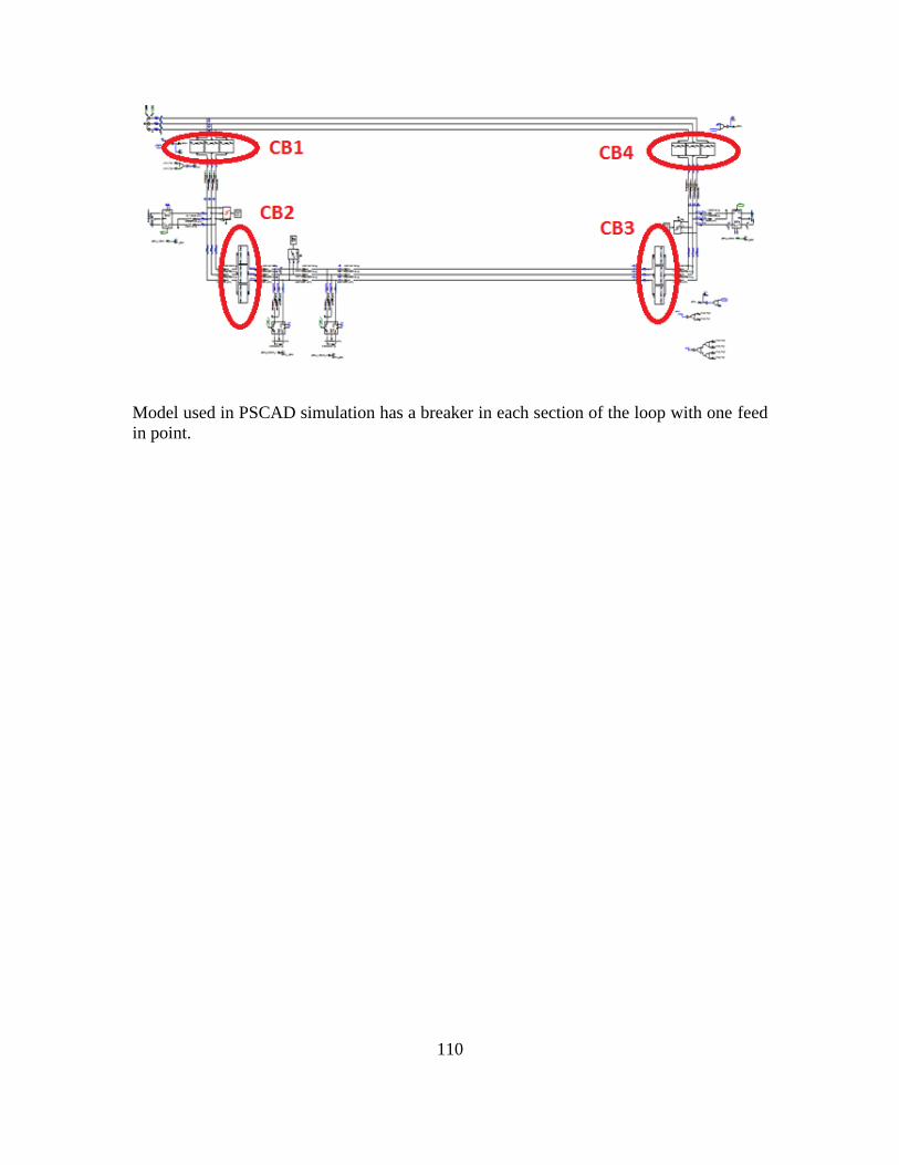
110
Model used in PSCAD simulation has a breaker in each section of the loop with one feed
in point.

111
APPENDIX B
SVP CONFIGURATOR PROGRAM
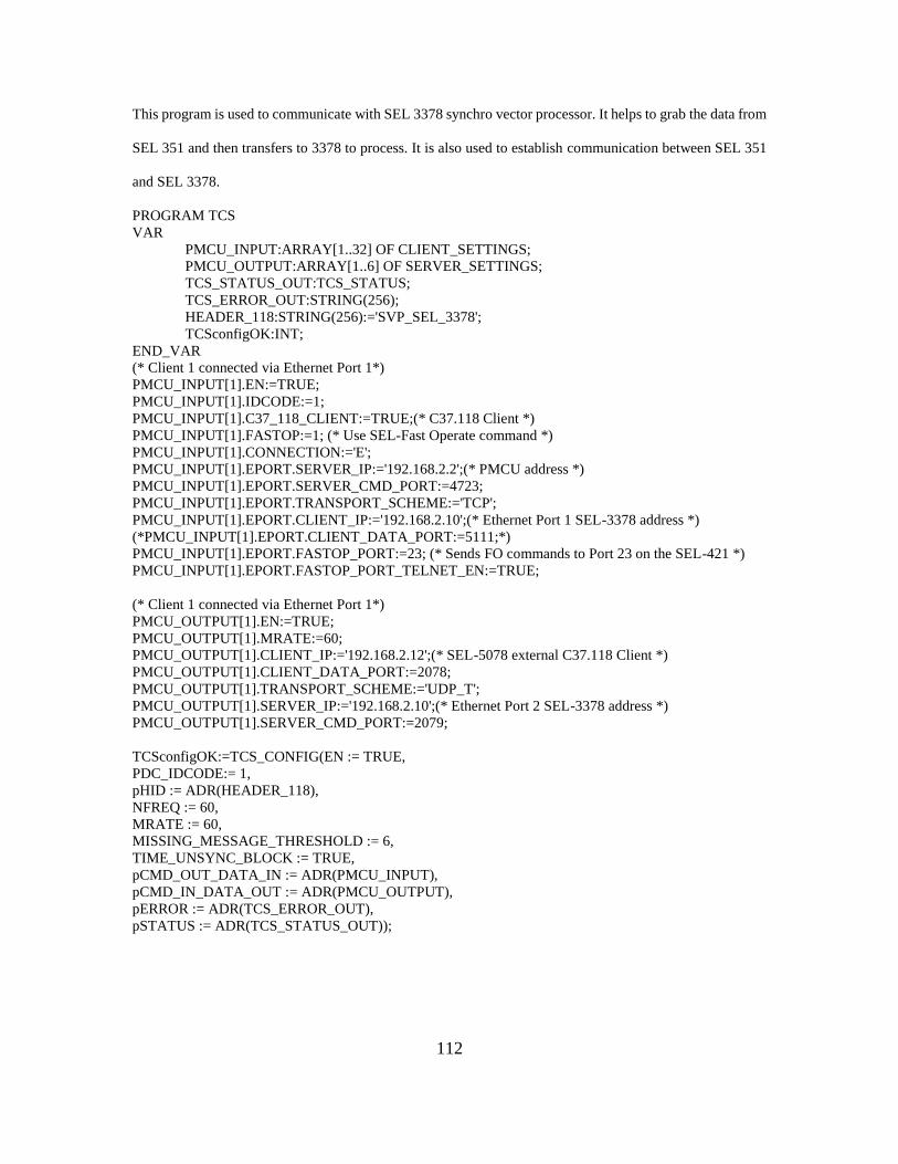
112
This program is used to communicate with SEL 3378 synchro vector processor. It helps to grab the data from
SEL 351 and then transfers to 3378 to process. It is also used to establish communication between SEL 351
and SEL 3378.
PROGRAM TCS
VAR
PMCU_INPUT:ARRAY[1..32] OF CLIENT_SETTINGS;
PMCU_OUTPUT:ARRAY[1..6] OF SERVER_SETTINGS;
TCS_STATUS_OUT:TCS_STATUS;
TCS_ERROR_OUT:STRING(256);
HEADER_118:STRING(256):='SVP_SEL_3378';
TCSconfigOK:INT;
END_VAR
(* Client 1 connected via Ethernet Port 1*)
PMCU_INPUT[1].EN:=TRUE;
PMCU_INPUT[1].IDCODE:=1;
PMCU_INPUT[1].C37_118_CLIENT:=TRUE;(* C37.118 Client *)
PMCU_INPUT[1].FASTOP:=1; (* Use SEL-Fast Operate command *)
PMCU_INPUT[1].CONNECTION:='E';
PMCU_INPUT[1].EPORT.SERVER_IP:='192.168.2.2';(* PMCU address *)
PMCU_INPUT[1].EPORT.SERVER_CMD_PORT:=4723;
PMCU_INPUT[1].EPORT.TRANSPORT_SCHEME:='TCP';
PMCU_INPUT[1].EPORT.CLIENT_IP:='192.168.2.10';(* Ethernet Port 1 SEL-3378 address *)
(*PMCU_INPUT[1].EPORT.CLIENT_DATA_PORT:=5111;*)
PMCU_INPUT[1].EPORT.FASTOP_PORT:=23; (* Sends FO commands to Port 23 on the SEL-421 *)
PMCU_INPUT[1].EPORT.FASTOP_PORT_TELNET_EN:=TRUE;
(* Client 1 connected via Ethernet Port 1*)
PMCU_OUTPUT[1].EN:=TRUE;
PMCU_OUTPUT[1].MRATE:=60;
PMCU_OUTPUT[1].CLIENT_IP:='192.168.2.12';(* SEL-5078 external C37.118 Client *)
PMCU_OUTPUT[1].CLIENT_DATA_PORT:=2078;
PMCU_OUTPUT[1].TRANSPORT_SCHEME:='UDP_T';
PMCU_OUTPUT[1].SERVER_IP:='192.168.2.10';(* Ethernet Port 2 SEL-3378 address *)
PMCU_OUTPUT[1].SERVER_CMD_PORT:=2079;
TCSconfigOK:=TCS_CONFIG(EN := TRUE,
PDC_IDCODE:= 1,
pHID := ADR(HEADER_118),
NFREQ := 60,
MRATE := 60,
MISSING_MESSAGE_THRESHOLD := 6,
TIME_UNSYNC_BLOCK := TRUE,
pCMD_OUT_DATA_IN := ADR(PMCU_INPUT),
pCMD_IN_DATA_OUT := ADR(PMCU_OUTPUT),
pERROR := ADR(TCS_ERROR_OUT),
pSTATUS := ADR(TCS_STATUS_OUT));
113
APPENDIX C
GENERATOR AND SYSTEM DATA OF THE FREEDM LOOP MODELED ON
RTDS USED IN VALIDATING THE PILOT DIRCETIONAL SCHEME

114
S-base = 2.5 MVA (2MVA at 0.8 pf Continuous)
Rated L-L RMS = 600V
Frequency = 60 Hz
Inertia Constant = 1.442 MW-s/MVA
Xa = 0.02 pu (Stator Reactance)
Xd = 3.145 pu (D-axis Unsaturated Reactance)
Xd' = 0.190 pu (D-axis Unsaturated Transient Reactance)
Xd" = 0.132 pu (D-axis Unsaturated Sub-Transient Reactance)
Xq = 1.470 pu (Q-axis Unsaturated Reactance)
Xq' = 0.186 pu (Q-axis Unsaturated Transient Reactance)
Xq" = 0.117 pu (Q-axis Unsaturated Sub-Transient Reactance)
Ra = 0.0022072 pu (Stator Resistance)
Tdo' = 5.48 sec (D-axis Un-saturated Transient Open T Constant)
Tdo" = 0.05 sec (D-axis Un-saturated Sub-Transient Open T Constant)
Tqo' = 0.85 sec (Q-axis Un-saturated Transient Open T Constant)
Tqo" = 0.05 sec (Q-axis Un-saturated Sub-Transient Open T Constant)
Machine Zero Sequence Resistance: 0.0004 pu
Machine Zero Sequence Reactance 0.05 pu
Neutral Series Resistance: 1.0E5 pu
Neutral Series Reactance: 0.0 pu
Step-up Transformer parameters: 600V-12.47kV
MVA rating = 2.5
Pos. Seq. Resistance = 0.02 pu
Pos. Seq. Reactance = 0.04 pu

115
APPENDIX D
DETERMINING VOLTAGE PHASE DIFFERENCE BETWEEN PMU’S DURING
MAXIMUM POWER FLOW OF THE TRANSMISSION LINE

116
Figure D1 shows the FREEDM loop with 5 buses. Bus 1 is designated as slack bus and rest of the buses are
assumed to be located at each relay position. The total allowable power-flow (4.06+ 2i p.u) in each line is
designated as a load at each bus. The line impedance between the bus 2 and bus 3 is 0.01906 +0.01906i in
per unit, between bus 3 and bus 4 is 0.03812+0.03812i, between bus 4 and bus 5 is 0.01906+0.01906i,
between bus 5 and bus 1 is 0.01906+0.01906i on a base of 100 MVA and voltage base of 12.47 kV. The
source reactance is 0.02906i per unit. All the system data is fed into Power System Analysis Tool (PSAT) in
the form of a Matlab file.
Figure D1 FREEDM system used for determining voltage phase profile during maximum power-flow
Matlab code representing system data
Bus.con = [ ...
1 1.00 1.000 0.0 1 1;
2 1.00 1.000 0.0 1 1;
3 1.00 1.000 0.0 1 1;
4 1.00 1.000 0.0 1 1;
5 1.00 1.000 0.0 1 1;
];
SW.con = [ ...
1 100.0 1.00 1.00000 0.00000 0.00000 0.00000 1.1 0.9 0.00000 1 1 1;
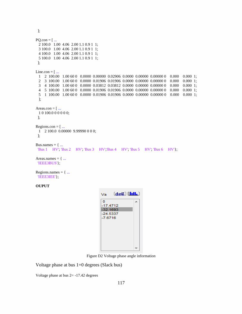
117
];
PQ.con = [ ...
2 100.0 1.00 4.06 2.00 1.1 0.9 1 1;
3 100.0 1.00 4.06 2.00 1.1 0.9 1 1;
4 100.0 1.00 4.06 2.00 1.1 0.9 1 1;
5 100.0 1.00 4.06 2.00 1.1 0.9 1 1;
];
Line.con = [ ...
1 2 100.00 1.00 60 0 0.0000 0.00000 0.02906 0.0000 0.00000 0.00000 0 0.000 0.000 1;
2 3 100.00 1.00 60 0 0.0000 0.01906 0.01906 0.0000 0.00000 0.00000 0 0.000 0.000 1;
3 4 100.00 1.00 60 0 0.0000 0.03812 0.03812 0.0000 0.00000 0.00000 0 0.000 0.000 1;
4 5 100.00 1.00 60 0 0.0000 0.01906 0.01906 0.0000 0.00000 0.00000 0 0.000 0.000 1;
5 1 100.00 1.00 60 0 0.0000 0.01906 0.01906 0.0000 0.00000 0.00000 0 0.000 0.000 1;
];
Areas.con = [ ...
1 0 100.0 0 0 0 0 0;
];
Regions.con = [ ...
1 2 100.0 0.00000 9.99990 0 0 0;
];
Bus.names = { ...
'Bus 1 HV'; 'Bus 2 HV'; 'Bus 3 HV';'Bus 4 HV'; 'Bus 5 HV'; 'Bus 6 HV'};
Areas.names = { ...
'IEEE3BUS'};
Regions.names = { ...
'IEEE3IEE'};
OUPUT
Figure D2 Voltage phase angle information
Voltage phase at bus 1=0 degrees (Slack bus)
Voltage phase at bus 2= -17.42 degrees
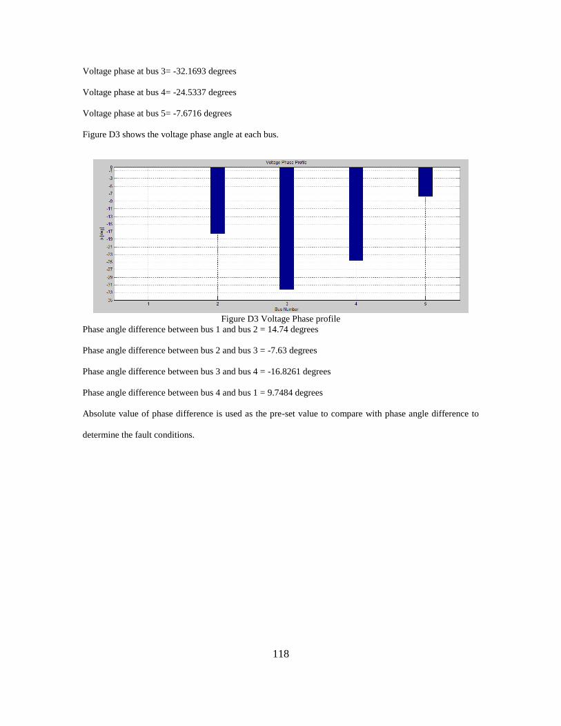
118
Voltage phase at bus 3= -32.1693 degrees
Voltage phase at bus 4= -24.5337 degrees
Voltage phase at bus 5= -7.6716 degrees
Figure D3 shows the voltage phase angle at each bus.
Figure D3 Voltage Phase profile
Phase angle difference between bus 1 and bus 2 = 14.74 degrees
Phase angle difference between bus 2 and bus 3 = -7.63 degrees
Phase angle difference between bus 3 and bus 4 = -16.8261 degrees
Phase angle difference between bus 4 and bus 1 = 9.7484 degrees
Absolute value of phase difference is used as the pre-set value to compare with phase angle difference to
determine the fault conditions.