DESIGN AND DEVELOPMENT OF A CONTINUOUS, OPEN-RETURN TRANSONIC

WIND TUNNEL FACILITY

BY

CODY GRAY

THESIS

Submitted in partial fulfillment of the requirements

for the degree of Master of Science in Aerospace Engineering

in the Graduate College of the

University of Illinois at Urbana-Champaign, 2017

Urbana, Illinois

Adviser:

Assistant Professor Phillip J. Ansell

ii

Abstract

A new transonic wind tunnel facility was designed and built on the University of Illinois

at Urbana-Champaign campus to enhance testing capabilities of the transonic flow regime. The

new tunnel will expand the experimental capabilities available to the Department of Aerospace

Engineering at UIUC for studying and understanding topics such as compressible dynamic stall

aerodynamics, shock buffet phenomenon and control, shock wave boundary layer ingestion to a

propulsor, and other future research topics.

The new wind tunnel is a rectangular testing facility with a 6 in (width) x 9 in (height)

cross-sectional area in the test section. It is a continuous, open-return facility, capable of operating

within a Mach number range of M=0-0.8, and possibly reaching M=0.85 or higher depending on

the test section configuration. The wind tunnel was assembled and installed in the Aerodynamics

Research Laboratory. The tunnel is driven by a centrifugal blower that exhausts the air back into

the laboratory. The components designed for the tunnel were the nozzle, diffuser, test section,

settling chamber, inlet flow conditioning section, and the structural assembly.

The most significant challenges in the design and development of the tunnel were

enveloped in the test section and suction plenum control system. When performing experiments

on transonic aerodynamic bodies, if the Mach number is high enough, pockets of locally

supersonic flow will be seen in the test section. Therefore, to simulate unbounded transonic flight,

partially-open test section walls were implemented to prevent shock reflections and test section

choking. The suction across these walls was controlled by flaps at the aft end of the test section.

The pressure differential created across the open-area walls can cause vibrational issues if adequate

suction is not provided and unloaded into the diffuser via control flaps. For this reason, thicker

open-area walls were substituted after the testing with thinner walls experienced these undesirable

vibrations.

iii

Acknowledgements

This project would not be complete without the support and guidance that I received from

my adviser Prof. Phil Ansell. He has been incredibly helpful throughout the design and

development process and I have enjoyed my time working under his supervision.

I would like to thank my family for all the love and support they have shown me throughout

my time here at UIUC. I am forever grateful for my family and I hope to make you all proud in

the next steps of my career. I would also like to thank Prof. Jim Leylek from the University of

Arkansas for all the guidance through my final undergraduate years, especially for convincing me

to apply to his alma mater, UIUC.

I am also grateful to the machine shop guys, Greg, Lee, Steve, and Dustin, without whom

this tunnel could not have been built. Finally, I would like to thank all the members for the

aerodynamics research group, especially Aaron Perry, for all the help during the completion of

this project.

iv

Table of Contents List of Figures ................................................................................................................................ vi

List of Tables .................................................................................................................................. x

Nomenclature ................................................................................................................................. xi

Chapter 1: Introduction ................................................................................................................... 1

1.1 Transonic Wind Tunnel Background .................................................................................... 1

1.2 Transonic Wind Tunnel Design Challenges.......................................................................... 3

1.3 Research Motivation ............................................................................................................. 5

Chapter 2: Design ........................................................................................................................... 7

2.1 Driving Design Factors ......................................................................................................... 7

2.1.1 Centrifugal Blower Selection ......................................................................................... 7

2.1.2 Test Section Size Selection........................................................................................... 10

2.2 Nozzle Inlet ......................................................................................................................... 12

2.2.1 Contraction Ratio .......................................................................................................... 12

2.2.2 Match Point of Nozzle Contraction .............................................................................. 14

2.3 Settling Chamber ................................................................................................................. 17

2.3.1 Honeycomb Flow Straightener ..................................................................................... 18

2.3.2 Turbulence-Reducing Screens ...................................................................................... 20

2.3.3 Settling Chamber Manufacturing ................................................................................. 22

2.4 Diffuser................................................................................................................................ 27

2.4.1 Diffuser Expansion Angle ............................................................................................ 28

2.4.2 Diffuser Material and Manufacturing ........................................................................... 29

2.5 Test Section ......................................................................................................................... 32

2.5.1 Open-area Walls ........................................................................................................... 33

2.5.2 Suction Plenums ........................................................................................................... 38

2.5.3 Suction Control ............................................................................................................. 39

2.5.4 Choke Vanes ................................................................................................................. 41

2.5.5 Walls ............................................................................................................................. 43

2.5.6 Windows ....................................................................................................................... 45

2.5.7 Model Mounting Apparatus.......................................................................................... 47

2.5.8 Stepper Motor Selection ............................................................................................... 50

v

2.6 Data Acquisition Capabilities ............................................................................................. 50

2.6.1 Mach Number Control via Static Pressure Taps and Thermocouple ........................... 50

2.6.2 PIV ................................................................................................................................ 53

2.6.3 Suction Control via Static Pressure Taps ..................................................................... 54

2.7 Structural Assembly ............................................................................................................ 54

2.7.1 Material and Manufacturing ......................................................................................... 55

2.7.2 Leveling ........................................................................................................................ 55

2.8 Transition Modifications ..................................................................................................... 58

Chapter 3: Results and Discussion ................................................................................................ 60

3.1 Wind Tunnel Performance Characteristics ......................................................................... 60

3.2 CFD Analysis ...................................................................................................................... 62

Chapter 4: Summary and Conclusions .......................................................................................... 72

APPENDIX A: TECHNICAL DOCUMENTATION .................................................................. 74

APPENDIX B: ENGINEERING DRAWINGS ........................................................................... 76

References ................................................................................................................................... 104

vi

List of Figures

Fig. 1.1 a) Airfoil in subsonic flow regime; b) airfoil in transonic flow regime; c) airfoil in

supersonic flow regime.2 ................................................................................................................. 2

Fig. 1.2 Transonic wind tunnel schematic. ..................................................................................... 3

Fig. 1.3 a) Slanted walls test section configuration; b) slotted walls test section configuration; c)

perforated walls test section configuration.1 ................................................................................... 4

Fig. 2.1 Comparison of pressure recovery and volume flow envelopes for a notional axial fan and

centrifugal blower. .......................................................................................................................... 8

Fig. 2.2 Performance curve of AirPro Fan model 420, sized for transonic wind tunnel. ............... 9

Fig. 2.3 a) AirPro blower system; b) ABB VFD. ......................................................................... 10

Fig. 2.4 a) Inlet nozzle side view; b) inlet nozzle isometric view. ............................................... 12

Fig. 2.5 3D inlet geometry for calculating contraction ratio.9 ...................................................... 13

Fig. 2.6 Schematic of match point location.10 ............................................................................... 14

Fig. 2.7 a) Entrance velocity variation chart; b) exit velocity variation chart; c) entrance pressure

coefficient chart; d) exit pressure coefficient chart.10 ................................................................... 16

Fig. 2.8 3D CAD model of settling chamber. ............................................................................... 18

Fig. 2.9 a) Circular honeycomb; b) square honeycomb; c) hexagonal honeycomb.20 .................. 19

Fig. 2.10 Settling chamber panels with slots: top and bottom walls. ............................................ 22

Fig. 2.11 Screen tensioning system............................................................................................... 23

Fig. 2.12 a) Turbulence screen assembly; b) screen L-stock and flatbar frame. .......................... 24

Fig. 2.13 a) Honeycomb assembly; b) honeycomb L-stock frame. .............................................. 24

Fig. 2.14 Settling chamber corner bracket. ................................................................................... 25

Fig. 2.15 a) PVC entrance; b) PVC entrance attached to settling chamber. ................................. 26

Fig. 2.16 a) Settling chamber access door; b) bolting bracket to seal access door. ...................... 27

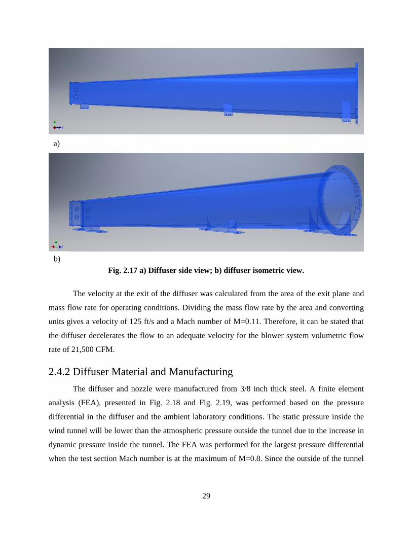
Fig. 2.17 a) Diffuser side view; b) diffuser isometric view. ......................................................... 29

Fig. 2.18 Diffuser FEA: Von Mises stress. ................................................................................... 31

Fig. 2.19 Diffuser FEA: displacement in X-direction. .................................................................. 31

Fig. 2.20 3D isometric view of test section. ................................................................................. 32

Fig. 2.21 a) Mach number distribution with perforated walls; b) Mach number distribution with

slotted walls. ................................................................................................................................. 34

vii

Fig. 2.22 Comparison of perforated walls with straight holes and inclined holes at different open-

area ratios.1 .................................................................................................................................... 35

Fig. 2.23 Cross-flow characteristics of perforated walls with 60 degree inclined holes for various

ratios of hole diameter to wall thickness, open-area ratio 6% at M=0.90.1 .................................. 35

Fig. 2.24 Hole inclination orientation.1 ......................................................................................... 36

Fig. 2.25 Porous plate model. ....................................................................................................... 37

Fig. 2.26 Porous plate with laser slot and static pressure ports. ................................................... 37

Fig. 2.27 Suction plenum attached to test section. ........................................................................ 38

Fig. 2.28 Plenum to diffuser gap. .................................................................................................. 39

Fig. 2.29 Suction plenum equipped with laser sheet window....................................................... 39

Fig. 2.30 Diffuser suction control flaps schematic.1 ..................................................................... 40

Fig. 2.31 Diffuser suction control flap design cross section. ........................................................ 41

Fig. 2.32 3D model of choke vane mechanism. ............................................................................ 42

Fig. 2.33 a) Choke vane top view; b) choke vane side view. ....................................................... 42

Fig. 2.34 Isometric view of test section walls. .............................................................................. 44

Fig. 2.35 Custom square tube bolting bracket. ............................................................................. 44

Fig. 2.36 Rectangular plate moment factor.5 ................................................................................ 45

Fig. 2.37 Test section side wall window. ...................................................................................... 46

Fig. 2.38 Laser sheet window. ...................................................................................................... 47

Fig. 2.39 Airfoil mount FEA: displacement in the Y-direction. ................................................... 48

Fig. 2.40 Airfoil mount apparatus. ................................................................................................ 49

Fig. 2.41 Test section pressure transducer and tap. ...................................................................... 52

Fig. 2.42 LabVIEW data acquisition block diagram. ................................................................... 53

Fig. 2.43 LabVIEW front panel for Mach number calculation. .................................................... 53

Fig. 2.44 LabVIEW front panel for test section temperature, speed of sound, and velocity

calculation. .................................................................................................................................... 53

Fig. 2.45 Static pressure tabs on both sides of porous wall. ......................................................... 54

Fig. 2.46 Structural assembly........................................................................................................ 55

Fig. 2.47 Custom leveling bolt assembly for settling chamber support........................................ 56

Fig. 2.48 Leveling mount for nozzle and diffuser. ....................................................................... 57

Fig. 2.49 Vibration-damping leveling mounts for blower assembly. ........................................... 58

viii

Fig. 2.50 Nozzle to test section transition with gap. ..................................................................... 59

Fig. 2.51 Nozzle to test section transition after smoothing process.............................................. 59

Fig. 3.1 Mach number distribution vs fan RPM. .......................................................................... 61

Fig. 3.2 CFD inlet boundary condition. ........................................................................................ 63

Fig. 3.3 CFD outlet boundary condition. ...................................................................................... 63

Fig. 3.4 CFD wall boundary condition. ........................................................................................ 64

Fig. 3.5 CFD viscous model. ........................................................................................................ 65

Fig. 3.6 a) CFD solution initialization; b) CFD reference values. ................................................ 66

Fig. 3.7 CFD velocity magnitude along centerline plane in streamwise downstream Z-direction.

....................................................................................................................................................... 67

Fig. 3.8 CFD velocity along centerline plane in streamwise downstream Z-direction. ................ 68

Fig. 3.9 CFD velocity along centerline plane in vertical Y-direction. .......................................... 68

Fig. 3.10 CFD velocity magnitude for full 3D tunnel mesh. ........................................................ 69

Fig. 3.11 CFD velocity magnitude on centerline plane in streamwise downstream Z-direction,

displaying the boundary layer. ...................................................................................................... 69

Fig. 3.12 CFD static pressure along centerline plane in streamwise downstream Z-direction. .... 70

Fig. 3.13 CFD static pressure plot along centerline plane in streamwise downstream Z-direction.

....................................................................................................................................................... 70

Fig. 3.14 CFD static pressure plot along walls in streamwise downstream Z-direction. ............. 70

Fig. 3.15 CFD residuals plot to show converging solution. .......................................................... 71

Fig. A. 1 AirPro dimension diagram.7............................................................................................ 74

Fig. A. 2 ABB ACS880 VFD dimensions. .................................................................................... 75

Fig. B. 1 Test section side wall connector, nozzle side. ................................................................ 76

Fig. B. 2 Test section side wall connector, diffuser side. .............................................................. 77

Fig. B. 3 Test section to nozzle flange. .......................................................................................... 78

Fig. B. 4 Test section side wall. ..................................................................................................... 79

Fig. B. 5 Test section top and bottom upstream wall. ................................................................... 80

Fig. B. 6 Test section to diffuser flange. ........................................................................................ 81

Fig. B. 7 Test section window frame. ............................................................................................ 82

Fig. B. 8 Test section window frame with isometric view. ........................................................... 83

Fig. B. 9 Test section window glass. ............................................................................................. 84

ix

Fig. B. 10 Diffuser. ....................................................................................................................... 85

Fig. B. 11 Nozzle front and side. ................................................................................................... 86

Fig. B. 12 Nozzle back and bottom. .............................................................................................. 87

Fig. B. 13 Choke vane. .................................................................................................................. 88

Fig. B. 14 Suction control flaps. .................................................................................................... 89

Fig. B. 15 Airfoil mount. ............................................................................................................... 90

Fig. B. 16 Motor mount left. .......................................................................................................... 91

Fig. B. 17 Motor mount left. .......................................................................................................... 92

Fig. B. 18 Motor mount extension. ................................................................................................ 93

Fig. B. 19 Motor mount right. ....................................................................................................... 94

Fig. B. 20 Motor mount right. ....................................................................................................... 95

Fig. B. 21 Laser sheet window frame. ........................................................................................... 96

Fig. B. 22 Laser sheet window frame with isometric view. .......................................................... 97

Fig. B. 23 Laser sheet window glass. ............................................................................................ 98

Fig. B. 24 Porous plate. ................................................................................................................. 99

Fig. B. 25 Porous plate with slot. ................................................................................................. 100

Fig. B. 26 Suction plenum. .......................................................................................................... 101

Fig. B. 27 Suction plenum with isometric view. .......................................................................... 102

Fig. B. 28 Suction plenum for laser sheet side. ............................................................................ 103

x

List of Tables

Table 1.1 Comparison of new transonic wind tunnel and existing university facilities. ................ 6

Table 2.1 Screen configurations.11 ................................................................................................ 21

Table 3.1 Transonic wind tunnel performance characteristics. .................................................... 61

Table 3.2 Coefficients for Mach number distribution trend lines. ................................................ 62

xi

Nomenclature

List of Symbols

a speed of sound

A cross-section area

Ad,e cross-section area of the diffuser exit plane

Ats cross-section area of the wind tunnel test section

A* cross-section area at choked conditions

β porosity or open-area ratio

B moment factor

CD wing drag coefficient

CL wing lift coefficient

Cp pressure coefficient

D drag force or diameter

DH hydraulic diameter

∆𝑝 pressure change

e exit plane

𝜀0𝑒𝑞 equivalent free-stream turbulence

𝜀𝑠∗ intrinsic turbulence created by the screen in the optimum position

𝜀∗ minimum value of turbulence

γ specific heat ratio

H height

i inlet plane

k pressure drop coefficient

Kh pressure loss coefficent

L lift force or length

�̇� mass flow rate

M Mach number

Mmax maximum moment

M∞ free stream Mach number

p unit pressure

xii

P static pressure

PT total pressure

q dynamic pressure

q∞ free-steam dynamic pressure

ρ density

R universal gas constant

s length of short side

S airfoil reference area

Smax maximum allowable stress

t window thickness

T static temperature

TT total temperature

U mean velocity

Um average velocity

�̃� percentage of maximum variation in velocity

V velocity

Vcl centerline velocity

Vcor velocity at corners

Vd,e velocity at the diffuser exit plane

Vmax maximum velocity

Vmin minimum velocity

Vts test section velocity

�̇� volumetric flow rate

W width

xiii

List of Abbreviations

AoA angle of attack

CAD computer aided design

CFD computational fluid dynamics

CFM cubic feet per minute

CR contraction ratio

FEA finite element analysis

hp horse power

ID inside diameter

OD outer diameter

PIV particle image velocimetry

psi pounds per square inch

RPM revolutions per minute

RTV room temperature vulcanization

SIS shock-induced separation

VFD variable frequency drive

1

Chapter 1

Introduction

Transonic wind tunnel testing encompasses the speed range between Mach 0.8-1.2, the

transition between subsonic to supersonic speeds. Operation so close to the speed of sound, M=1.0,

presents unusual challenges both in the design of aircraft and wind tunnels.1 This difficulty is

caused by the aerodynamic phenomenon where the flow changes from a “single-type flow,” purely

subsonic or supersonic, to a “mixed-type flow” with local supersonic fields embedded in the

subsonic flow or vice versa.1 These complexities in the flow have made it impossible to establish

simple transonic theories that can be used to reliably predict the aerodynamic flow about a

transonic aircraft. The difficulties in theory stems from subsonic flows being based on elliptic

governing equations and supersonic flows being based on hyperbolic governing equations. Due to

these challenges, the study of aerodynamic geometries operating across the transonic speed range

relies heavily on wind tunnel experiments to acquire the performance and characterize the flow

field about aerodynamic bodies.

1.1 Transonic Wind Tunnel Background

Transonic wind tunnels provide a facility for examining the fluid mechanics and associated

phenomena for air traveling at the speed range when the transition from subsonic to supersonic

2

occurs. This speed range, as opposed to a low-speed tunnel, cannot be treated as incompressible,

and therefore compressibility effects must be taken into account. For a freestream Mach number

of 0.8, the density can change by up to 26%.1 When a model, such as an airfoil, is introduced into

the flow, shock waves can occur due to choking in the test section. The choking is caused by the

reduced area between the test section walls and the model. This can present difficulties that only

increase in severity as sonic unity is approached in the freestream flow, resulting in inaccurate data

if these considerations are not accounted for properly.

Shock waves can also occur in transonic flow due to acceleration over a surface. If the

freestream Mach number flowing over an airfoil is subsonic, but sufficiently near 1.0, the flow

acceleration over the top surface of the airfoil may result in a local supersonic region.2 When the

Mach number is high enough, it will produce a pocket of locally supersonic flow which terminates

with a shock wave, resulting in a discontinuous and sometimes severe change in flow properties.2

The flow then slows down to subsonic speeds downstream of the shockwave. This change in speed

regimes, along with little to no analytical theory available, brings experimental complications such

as test section wall boundary corrections, shock reflections, choking, and other phenomena.3 The

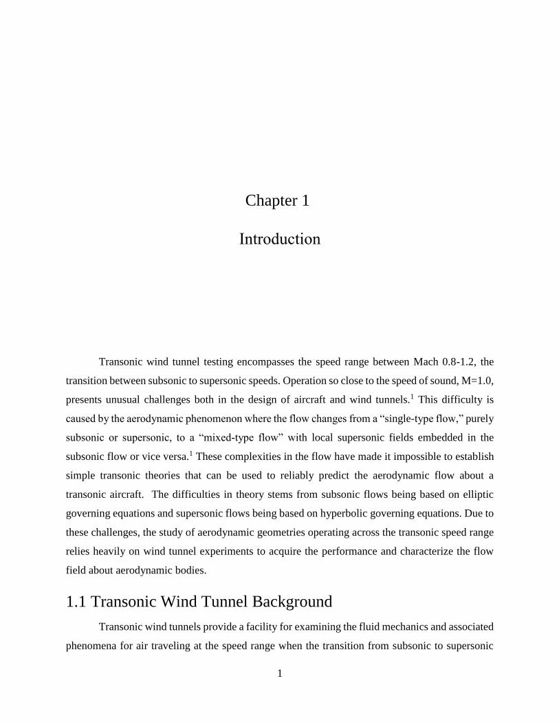
range at which this type of local supersonic flow occurs is between Mach 0.8 and 1.0 as shown in

Fig. 1.1 b). When the freestream velocity is below Mach 0.8 as shown in Fig. 1.1 a), the flow is

completely subsonic and a shock wave does not form. If the freestream velocity is increased to the

upper limits of the transonic speed range, above M∞=1, a bow shock will form upstream of the

leading edge and a trailing-edge shock will also form as shown in Fig. 1.1 c).

Fig. 1.1 a) Airfoil in subsonic flow regime; b) airfoil in transonic flow regime; c) airfoil in

supersonic flow regime.2

a) b)

c)

3

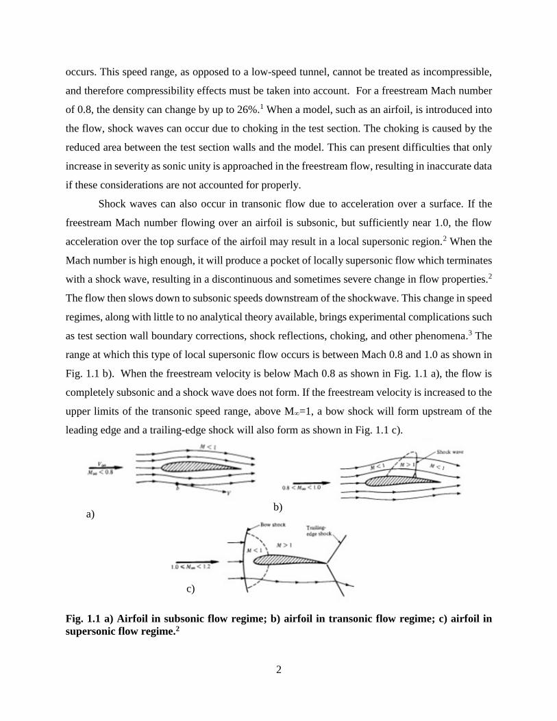
The three main components of a transonic wind tunnel design are the nozzle, test section,

and diffuser, as shown in the schematic in Fig. 1.2. This figure shows a continuous open-return

wind tunnel, as opposed to an intermittent blowdown tunnel. In a blowdown tunnel, a pressure

difference fore and aft of the test section is created by unloading a compressed air storage tank

down a series of pipes, resulting in high pressure upstream and low pressure downstream. In a

continuous open-return tunnel, the air is moved via a suction source (such as a blower or fan)

located at the downstream end. The nozzle is the stage where the flow is accelerated to the

transonic speed regime. The nozzle is configured such that flow entering is moving at a low

subsonic speed, M<<0.1. At the downstream end of the nozzle the flow reaches its desired speed,

based on the area ratio created from the nozzle contraction. The test section is the middle stage

and the flow remains constant and uniform throughout the length of the test section (given there is

no model present). The diffuser stage is where the flow velocity is decreased through expansion

by increasing the wind tunnel cross-sectional area with streamwise distance (following isentropic

flow theory), which results in an increase in pressure. The pressure difference required to run the

tunnel is driven by a centrifugal blower at the aft end of the diffuser. The shock waves mentioned

above will occur in the test section stage of the tunnel and the resulting pressure losses must be

able to be sustained by the blower driving the tunnel.

Fig. 1.2 Transonic wind tunnel schematic.

1.2 Transonic Wind Tunnel Design Challenges

The test section segment of a transonic wind tunnel is where most of the design challenges

occur. If a shock wave occurs in a test section with solid walls, the shock will reflect off of the

walls and back towards the model, potentially altering the flow about the test article. Such a case

4

would produce a flow field that is not a representation of what happens in unbounded transonic

flight, as the shock wave would continue to propagate throughout the atmosphere at the given

Mach angle. Special attention must be given to the walls above and below the model. For example,

if flow is going from left to right and the cross section of the airfoil is oriented horizontally, the

walls indicated would be the top and the bottom.

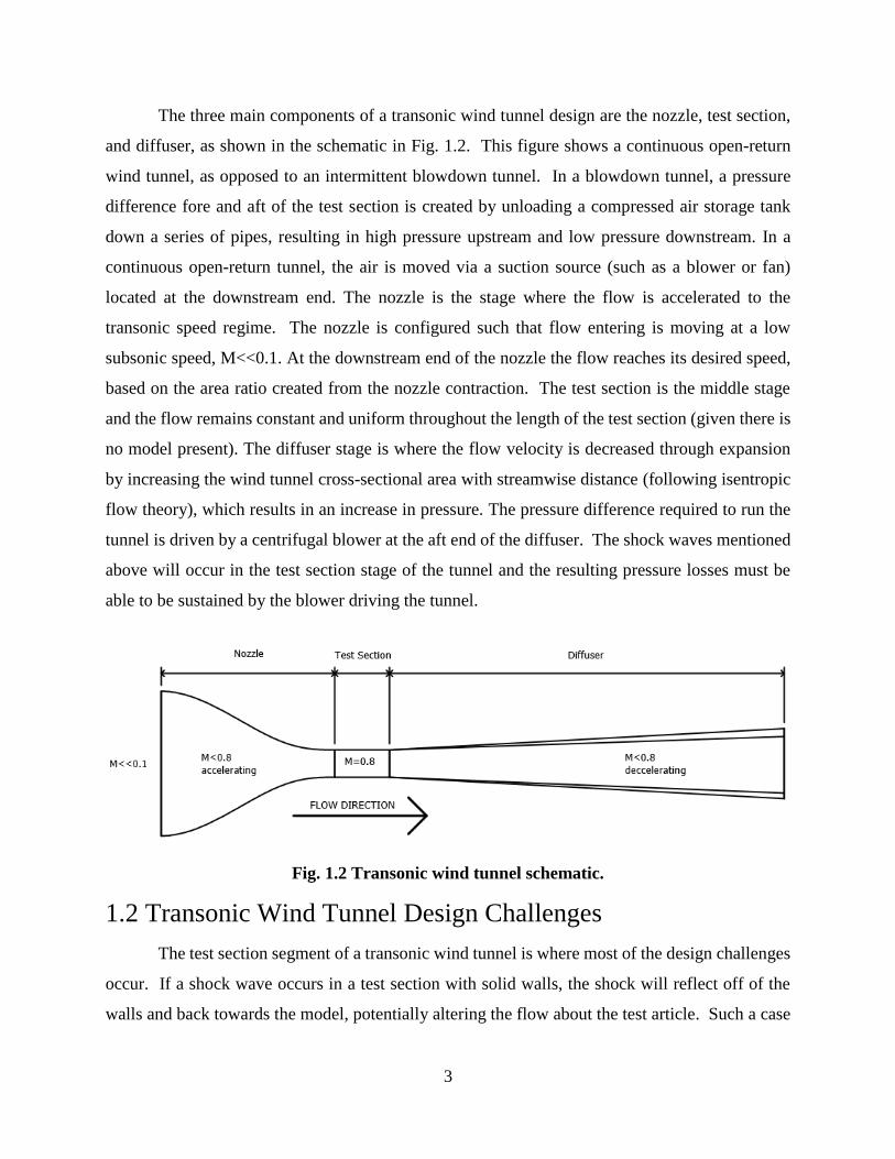
There are 3 main designs for test section walls, presented in Fig. 1.3, that help to alleviate

not only the reflection of shock waves, but also streamlines from the model that would not be

reflected in real flight: slanted walls, slotted walls, and perforated walls. The streamlines that flow

around any geometry, as shown in Fig. 1.1 a), b), and c), should follow their natural path without

external obstructions such as a wind tunnel wall.

Fig. 1.3 a) Slanted walls test section configuration; b) slotted walls test section configuration;

c) perforated walls test section configuration.1

The slanted wall design, as shown in Fig. 1.3 a), was the first one developed, it increased

the flow area aft of the throat that established supersonic flow in the test region.1 The test models

still had to remain very small to avoid shock reflection and therefore the design is not used today.

The slotted and perforated wall designs are similar in function, both bleed out the shocks and

streamlines into a pressure chamber in order to avoid reflections and/or choking. During low-speed

wind tunnel development in the 1930’s and later, it was shown that at the combination of both

solid and open walls could greatly reduce wind tunnel velocity corrections.1 These are inherent

velocity corrections in all wind tunnel testing due to wall interference. Due to these corrections

increasing with the third power of the Prandtl factor √(1 − 𝑀∞2 ), these open walls were necessary

to keep the corrections reasonably small.1 The basic configuration for slotted walls, as shown in

b) c) a)

5

Fig. 1.3 a), were longitudinal openings on the test section walls, running in-line with the

streamwise direction. Perforated walls, as shown in Fig. 1.3 c), have holes throughout the wall,

usually inclined towards the direction of the flow and offers a larger resistance to inflow back into

the test section. The flow into the suction plenum chamber is then routed back into the diffuser or

an external suction source. Along with alleviating shock wave and streamline reflections, both

configurations increase the available blockage, allowing larger models to be tested.1

The test section choking phenomenon is a serious problem when a model is introduced to

the flow. When solid test section walls are used, the amount of available blockage before choking

is relatively small, where the blockage represents the area occupied by the test article out of the

available test section cross sectional area. As the freestream velocity approaches sonic conditions,

the amount of blockage required to choke the flow approaches zero. Flow choking can be

addressed by using some of the same methods as dealing with shock wave reflections. The open

area of the walls effectively increases the flow area and discourages the flow from choking. This

choking can be restricted if enough of the excess mass flow can bypass the model by flowing out

of the slots or perforated holes.4 Another method used to control the Mach number and prevent

choking in the test section is the installation of choke tabs or choke vanes. These are located aft

of the test section, inside the diffuser, and are adjusted to be the smallest cross sectional area in the

tunnel. This guarantees that if choking does occur, it will be in line with the tabs rather than the

model in the test section. Although shock waves can occur, they should not be due to choking in

the test section because of area blockage. Rather, shock waves should naturally occur due to

expansion over the airfoil surface, creating a local supersonic region.

1.3 Research Motivation

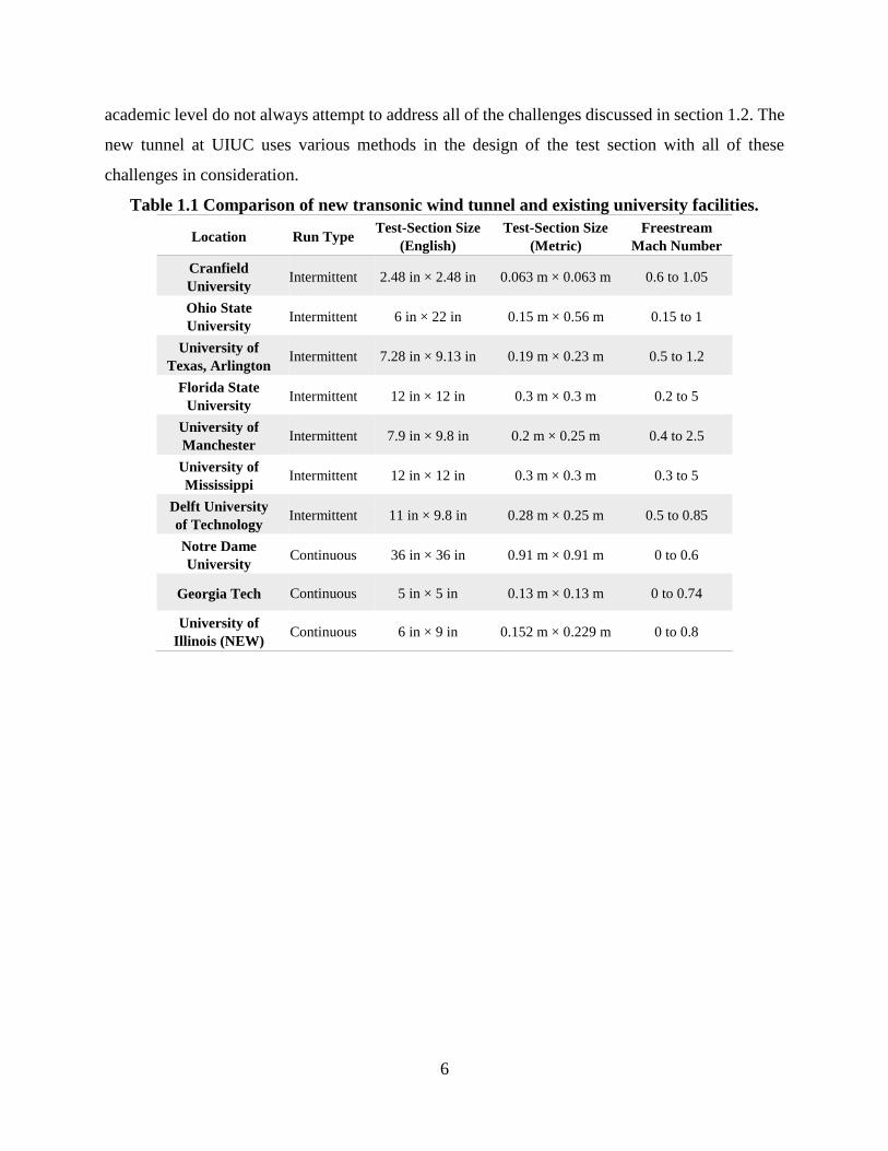
There are very few transonic wind tunnel facilities utilized at the academic level. A list of

these facilities is presented in Table 1.1. Given the analytical and computational limitations in the

transonic regime, wind tunnel experimentation is crucial to understanding transonic aerodynamics.

The focus on developing the transonic tunnel in this study is to allow further research in the

transonic flow regime to be conducted. This research includes but is not limited to: compressible

dynamic stall aerodynamics, testing various transonic airfoils for commercial aircraft, shock buffet

phenomenon and control, shock wave boundary layer ingestion to a propulsor, validation for

computational fluid dynamics, and shock-induced separation (SIS). Transonic wind tunnels at the

6

academic level do not always attempt to address all of the challenges discussed in section 1.2. The

new tunnel at UIUC uses various methods in the design of the test section with all of these

challenges in consideration.

Table 1.1 Comparison of new transonic wind tunnel and existing university facilities.

Location Run Type Test-Section Size

(English) Test-Section Size

(Metric) Freestream

Mach Number

Cranfield

University Intermittent 2.48 in × 2.48 in 0.063 m × 0.063 m 0.6 to 1.05

Ohio State

University Intermittent 6 in × 22 in 0.15 m × 0.56 m 0.15 to 1

University of

Texas, Arlington Intermittent 7.28 in × 9.13 in 0.19 m × 0.23 m 0.5 to 1.2

Florida State

University Intermittent 12 in × 12 in 0.3 m × 0.3 m 0.2 to 5

University of

Manchester Intermittent 7.9 in × 9.8 in 0.2 m × 0.25 m 0.4 to 2.5

University of

Mississippi Intermittent 12 in × 12 in 0.3 m × 0.3 m 0.3 to 5

Delft University

of Technology Intermittent 11 in × 9.8 in 0.28 m × 0.25 m 0.5 to 0.85

Notre Dame

University Continuous 36 in × 36 in 0.91 m × 0.91 m 0 to 0.6

Georgia Tech Continuous 5 in × 5 in 0.13 m × 0.13 m 0 to 0.74

University of

Illinois (NEW) Continuous 6 in × 9 in 0.152 m × 0.229 m 0 to 0.8

7

Chapter 2

Design

This chapter describes the component design of a transonic wind tunnel. It includes a

detailed design description of the following: nozzle, test section, diffuser, settling chamber,

blower, structure assembly, data acquisition, and post-manufacturing modifications.

2.1 Driving Design Factors

The key driving design factors for the transonic wind tunnel are as follows. The wind

tunnel must be able to produce uniform transonic flow at the design Mach number (M=0.8) in the

test section. The driving force of the tunnel, a centrifugal blower for this tunnel, must be

sufficiently large enough to sustain the corresponding mass flow rate and compensate for the

pressure losses that incur. The test section is constrained by the size of the blower, and the design

of all the other components of the wind tunnel are based on the size of the test section.

2.1.1 Centrifugal Blower Selection

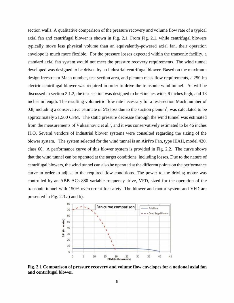
For a continuous transonic wind tunnel, axial compressor or centrifugal blower systems are

commonly used.5 These systems are capable of operating in the presence of the large total pressure

losses resulting from high-speed flows, shock structures, and suction across partially open test-

8

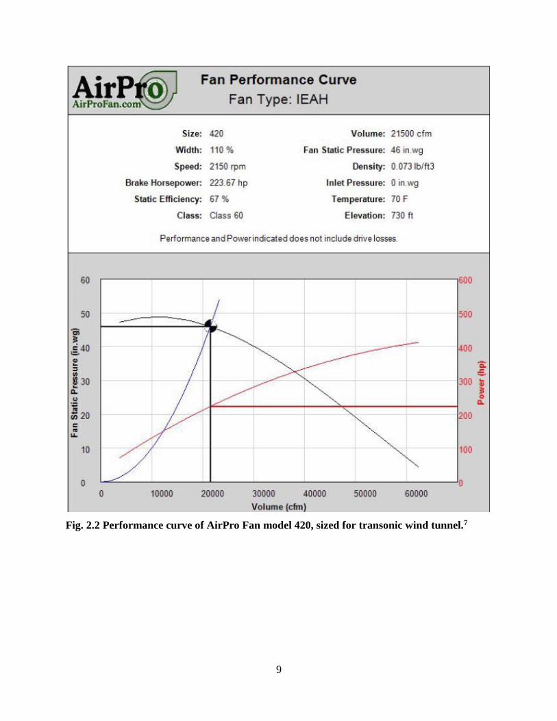
section walls. A qualitative comparison of the pressure recovery and volume flow rate of a typical

axial fan and centrifugal blower is shown in Fig. 2.1. From Fig. 2.1, while centrifugal blowers

typically move less physical volume than an equivalently-powered axial fan, their operation

envelope is much more flexible. For the pressure losses expected within the transonic facility, a

standard axial fan system would not meet the pressure recovery requirements. The wind tunnel

developed was designed to be driven by an industrial centrifugal blower. Based on the maximum

design freestream Mach number, test section area, and plenum mass flow requirements, a 250-hp

electric centrifugal blower was required in order to drive the transonic wind tunnel. As will be

discussed in section 2.1.2, the test section was designed to be 6 inches wide, 9 inches high, and 18

inches in length. The resulting volumetric flow rate necessary for a test-section Mach number of

0.8, including a conservative estimate of 5% loss due to the suction plenum1, was calculated to be

approximately 21,500 CFM. The static pressure decrease through the wind tunnel was estimated

from the measurements of Vukasinovic et al.6, and it was conservatively estimated to be 46 inches

H2O. Several vendors of industrial blower systems were consulted regarding the sizing of the

blower system. The system selected for the wind tunnel is an AirPro Fan, type IEAH, model 420,

class 60. A performance curve of this blower system is provided in Fig. 2.2. The curve shows

that the wind tunnel can be operated at the target conditions, including losses. Due to the nature of

centrifugal blowers, the wind tunnel can also be operated at the different points on the performance

curve in order to adjust to the required flow conditions. The power to the driving motor was

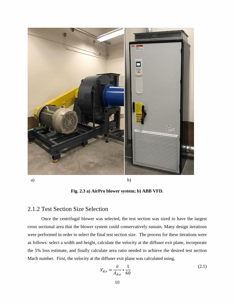
controlled by an ABB ACs 880 variable frequency drive, VFD, sized for the operation of the

transonic tunnel with 150% overcurrent for safety. The blower and motor system and VFD are

presented in Fig. 2.3 a) and b).

Fig. 2.1 Comparison of pressure recovery and volume flow envelopes for a notional axial fan

and centrifugal blower.

9

Fig. 2.2 Performance curve of AirPro Fan model 420, sized for transonic wind tunnel.7

10

Fig. 2.3 a) AirPro blower system; b) ABB VFD.

2.1.2 Test Section Size Selection

Once the centrifugal blower was selected, the test section was sized to have the largest

cross sectional area that the blower system could conservatively sustain. Many design iterations

were performed in order to select the final test section size. The process for these iterations were

as follows: select a width and height, calculate the velocity at the diffuser exit plane, incorporate

the 5% loss estimate, and finally calculate area ratio needed to achieve the desired test section

Mach number. First, the velocity at the diffuser exit plane was calculated using,

(2.1)

𝑉𝑑,𝑒 =�̇�

𝐴𝑑,𝑒∗

1

60

a) b)

11

where 𝑉𝑑,𝑒 denotes the velocity at the diffuser exit plane in ft/s, �̇� denotes the volumetric flow rate

of the blower in CFM, and 𝐴𝑑,𝑒 is the cross sectional area of the diffuser exit plane in ft2. The

Mach number at the diffuser exit plane with 5% loss estimate was calculated using,

(2.2)

where 𝑎 denotes the ambient speed of sound, 𝑎 = 1116.45 𝑓𝑡/𝑠. The Mach number at the diffuser

exit plane, 𝑀𝑑,𝑒 = 0.1, corresponds to an area ratio, relative to sonic conditions of 𝐴𝑑,𝑒/𝐴∗ =

5.8218 according to isentropic flow. The isentropic area ratio, relative to sonic conditions, for

M=0.8 in the test section is 𝐴𝑡𝑠/𝐴∗ = 1.038. Next, the area ratio between the diffuser exit plane

and the test section cross-sectional areas was calculated using,

(2.3)

which corresponds to an isentropic area ratio of 𝐴𝑑,𝑒/𝐴𝑡𝑠 = 5.609. The actual geometric area ratio

between the diffuser exit plane and test section was 𝐴𝑑,𝑒/𝐴𝑡𝑠 = 7.694. Therefore, since the actual

geometric area ratio was significantly larger than the estimated isentropic area ratio, it can be

conservatively stated that the area change in the diffuser was large enough for the wind tunnel to

reach the desired test section Mach number, as well as sustain unforeseen pressure losses. A

rectangular test section was selected to give more space between the model and the top and bottom

walls than that of a square test section, which reduced the influence of wall interference during

airfoil testing.

The length of the test section was designed based on an airfoil model with a 6 inch chord.

This corresponded to an aspect ratio of 1, assuming the model was installed horizontally. The

models will be mounted at the quarter-chord position and 5.5 inches downstream from the

beginning of the test section. According to Pope5, a test section length of at least 1.5 test section

heights should be adequate for the types of test in this tunnel. Also, Goett8 recommends at least

one chord length of test section behind the model to ensure flow stabilization for accurate pressure

measurements. Following the above criteria, the test section was designed at 18 inches (or 2 test

section heights), resulting in 8 inches of space (or 1.333 chord lengths) between the trailing edge

of the model (at 0° AoA) and the end of the test section.

𝑀𝑑,𝑒 =𝑉𝑑,𝑒

𝑎∗ 0.95

𝐴𝑑,𝑒/𝐴𝑡𝑠 =𝐴𝑑,𝑒/𝐴∗

𝐴𝑡𝑠/𝐴∗

12

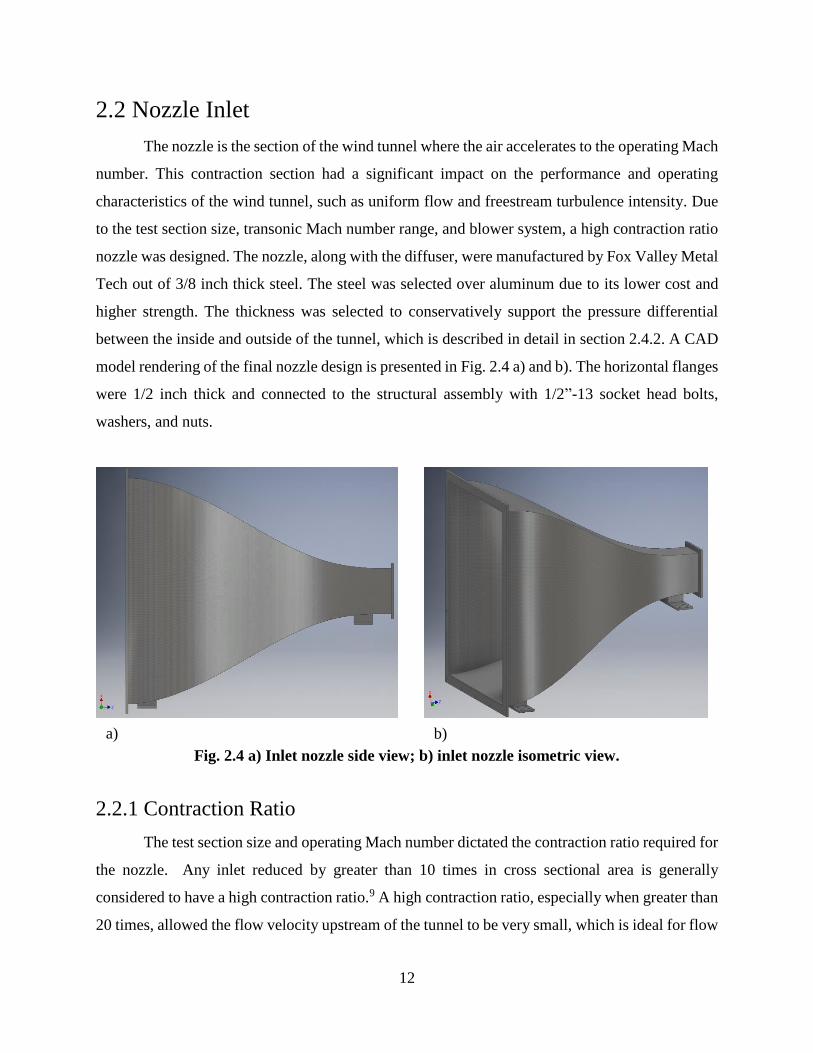
2.2 Nozzle Inlet

The nozzle is the section of the wind tunnel where the air accelerates to the operating Mach

number. This contraction section had a significant impact on the performance and operating

characteristics of the wind tunnel, such as uniform flow and freestream turbulence intensity. Due

to the test section size, transonic Mach number range, and blower system, a high contraction ratio

nozzle was designed. The nozzle, along with the diffuser, were manufactured by Fox Valley Metal

Tech out of 3/8 inch thick steel. The steel was selected over aluminum due to its lower cost and

higher strength. The thickness was selected to conservatively support the pressure differential

between the inside and outside of the tunnel, which is described in detail in section 2.4.2. A CAD

model rendering of the final nozzle design is presented in Fig. 2.4 a) and b). The horizontal flanges

were 1/2 inch thick and connected to the structural assembly with 1/2”-13 socket head bolts,

washers, and nuts.

Fig. 2.4 a) Inlet nozzle side view; b) inlet nozzle isometric view.

2.2.1 Contraction Ratio

The test section size and operating Mach number dictated the contraction ratio required for

the nozzle. Any inlet reduced by greater than 10 times in cross sectional area is generally

considered to have a high contraction ratio.9 A high contraction ratio, especially when greater than

20 times, allowed the flow velocity upstream of the tunnel to be very small, which is ideal for flow

a) b)

13

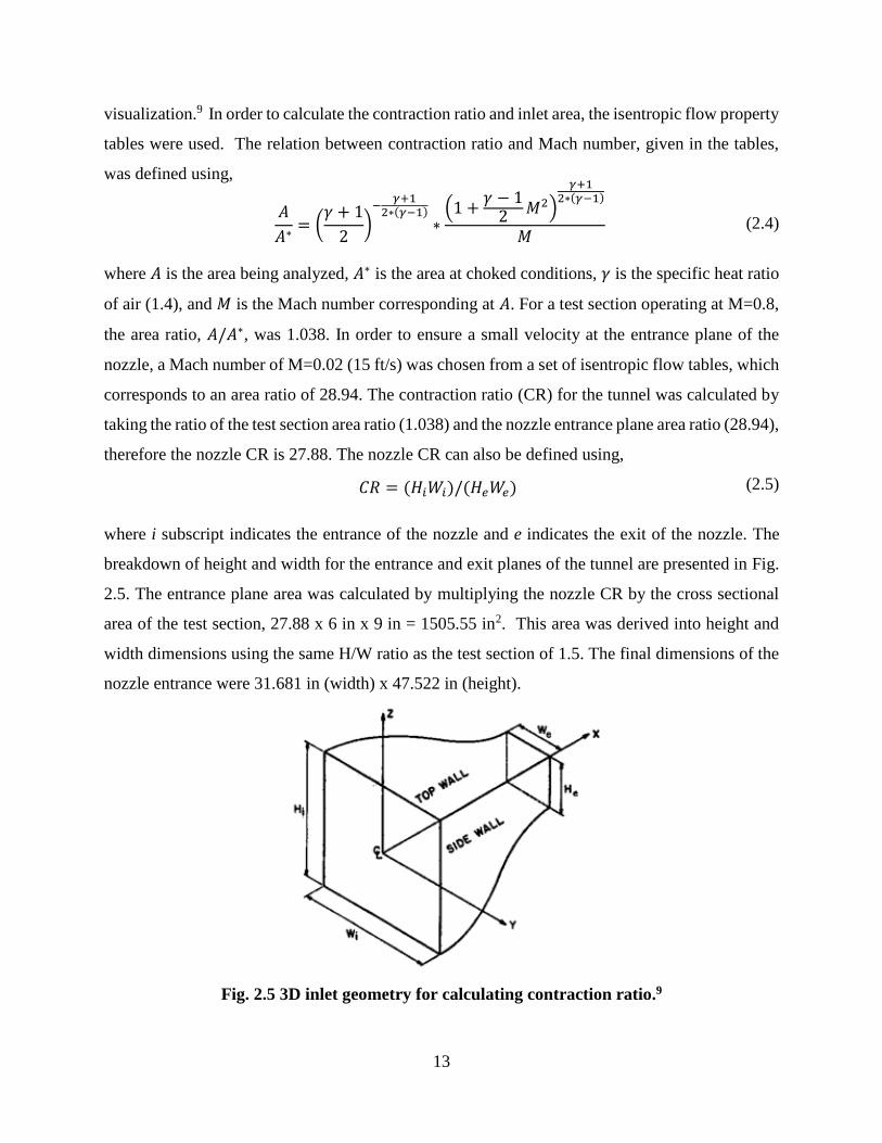
visualization.9 In order to calculate the contraction ratio and inlet area, the isentropic flow property

tables were used. The relation between contraction ratio and Mach number, given in the tables,

was defined using,

(2.4)

where 𝐴 is the area being analyzed, 𝐴∗ is the area at choked conditions, 𝛾 is the specific heat ratio

of air (1.4), and 𝑀 is the Mach number corresponding at 𝐴. For a test section operating at M=0.8,

the area ratio, 𝐴/𝐴∗, was 1.038. In order to ensure a small velocity at the entrance plane of the

nozzle, a Mach number of M=0.02 (15 ft/s) was chosen from a set of isentropic flow tables, which

corresponds to an area ratio of 28.94. The contraction ratio (CR) for the tunnel was calculated by

taking the ratio of the test section area ratio (1.038) and the nozzle entrance plane area ratio (28.94),

therefore the nozzle CR is 27.88. The nozzle CR can also be defined using,

(2.5)

where i subscript indicates the entrance of the nozzle and e indicates the exit of the nozzle. The

breakdown of height and width for the entrance and exit planes of the tunnel are presented in Fig.

2.5. The entrance plane area was calculated by multiplying the nozzle CR by the cross sectional

area of the test section, 27.88 x 6 in x 9 in = 1505.55 in2. This area was derived into height and

width dimensions using the same H/W ratio as the test section of 1.5. The final dimensions of the

nozzle entrance were 31.681 in (width) x 47.522 in (height).

Fig. 2.5 3D inlet geometry for calculating contraction ratio.9

𝐴

𝐴∗= (

𝛾 + 1

2)

−𝛾+1

2∗(𝛾−1)∗

(1 +𝛾 − 1

2 𝑀2)

𝛾+12∗(𝛾−1)

𝑀

𝐶𝑅 = (𝐻𝑖𝑊𝑖)/(𝐻𝑒𝑊𝑒)

14

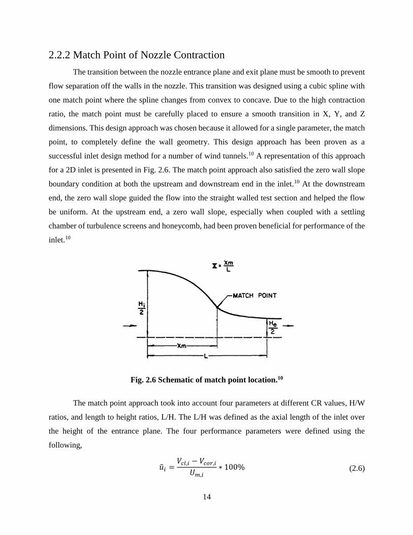
2.2.2 Match Point of Nozzle Contraction

The transition between the nozzle entrance plane and exit plane must be smooth to prevent

flow separation off the walls in the nozzle. This transition was designed using a cubic spline with

one match point where the spline changes from convex to concave. Due to the high contraction

ratio, the match point must be carefully placed to ensure a smooth transition in X, Y, and Z

dimensions. This design approach was chosen because it allowed for a single parameter, the match

point, to completely define the wall geometry. This design approach has been proven as a

successful inlet design method for a number of wind tunnels.10 A representation of this approach

for a 2D inlet is presented in Fig. 2.6. The match point approach also satisfied the zero wall slope

boundary condition at both the upstream and downstream end in the inlet.10 At the downstream

end, the zero wall slope guided the flow into the straight walled test section and helped the flow

be uniform. At the upstream end, a zero wall slope, especially when coupled with a settling

chamber of turbulence screens and honeycomb, had been proven beneficial for performance of the

inlet.10

Fig. 2.6 Schematic of match point location.10

The match point approach took into account four parameters at different CR values, H/W

ratios, and length to height ratios, L/H. The L/H was defined as the axial length of the inlet over

the height of the entrance plane. The four performance parameters were defined using the

following,

(2.6)

�̃�𝑖 =𝑉𝑐𝑙,𝑖 − 𝑉𝑐𝑜𝑟,𝑖

𝑈𝑚,𝑖∗ 100%

15

(2.7)

(2.8)

(2.9)

where �̃�𝑖 and �̃�𝑒 are the percent of maximum variation in velocity at the entrance and exit plane,

𝑉𝑐𝑙 is the centerline velocity, 𝑉𝑐𝑜𝑟 is the velocity at the corners, 𝑈𝑚 is the average velocity at either

the entrance or exit, 𝑐𝑝,𝑖 and 𝑐𝑝,𝑒 are the coefficients of pressure, and 𝑉𝑚𝑎𝑥 and 𝑉𝑚𝑖𝑛 are the

maximum and minimum speeds in the inlet.10 For each respective plane, 𝑉𝑐𝑙,𝑖

𝑈𝑚,𝑖 is the maximum and

𝑉𝑐𝑜𝑟,𝑖

𝑈𝑚,𝑖 is the minimum for the entrance, and

𝑉𝑐𝑜𝑟,𝑒

𝑈𝑚,𝑒 is the maximum and

𝑉𝑐𝑙,𝑒

𝑈𝑚,𝑒 is the minimum for the

exit. These four parameters define the aerodynamic performance of the inlet nozzle.10 In order to

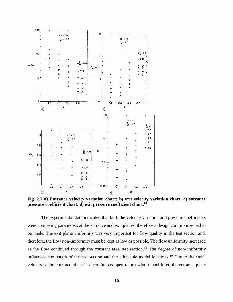
select the match point, inlet design charts generated from experimental data were referenced,

presented in Fig. 2.7 a) through d). The charts in Fig. 2.7, along with others at different CR and

H/W values, were interpolated to estimate the desired match point of the transonic wind tunnel

model at CR=27.88 and H/W of 1.5.

�̃�𝑒 =𝑉𝑐𝑜𝑟,𝑒 − 𝑉𝑐𝑙,𝑒

𝑈𝑚,𝑒∗ 100%

𝑐𝑝,𝑖 = 1 − (𝑉𝑚𝑖𝑛

𝑈𝑚,𝑖)

2

𝑐𝑝,𝑒 = 1 − (𝑈𝑚,𝑒

𝑉𝑚𝑎𝑥)

2

16

Fig. 2.7 a) Entrance velocity variation chart; b) exit velocity variation chart; c) entrance

pressure coefficient chart; d) exit pressure coefficient chart.10

The experimental data indicated that both the velocity variation and pressure coefficients

were competing parameters at the entrance and exit planes, therefore a design compromise had to

be made. The exit plane uniformity was very important for flow quality in the test section and,

therefore, the flow non-uniformity must be kept as low as possible. The flow uniformity increased

as the flow continued through the constant area test section.10 The degree of non-uniformity

influenced the length of the test section and the allowable model locations.10 Due to the small

velocity at the entrance plane in a continuous open-return wind tunnel inlet, the entrance plane

a) b)

c) d)

17

uniformity was not as critical of a parameter. It was possible to see speed variations of over 100%

of the mean value across the inlet plane in some tunnels.10 Although this parameter was less

critical, it can affect the size and placement of turbulence screens or honeycomb, or possibly set

an upper limit on tunnel operating speed.10 Therefore, both parameters should be kept at lower

values, with more emphasis put on the exit plan uniformity. A favorable pressure coefficient was

seen through the nozzle due the reduction in flow area and resulted in an increase in speed. The

pressure coefficients at the entrance and exit plane were competing in that the as the match point

was moved downstream, the pressure coefficient at the exit plane increased as the pressure

coefficients at the entrance plane decreased, as presented in Fig. 2.7 c) and d). From a favorable

pressure point of view, the match point was placed farther downstream to achieve a smoother

transition throughout the tunnel. The favorable pressure gradient was not as strong as an upstream

match point, but it extended over a greater length of the inlet. After interpolating the inlet design

charts, a match point of X=0.64 was selected for the transonic wind tunnel inlet. The

corresponding parameters at CR=27.88 and H/W=1.5 were as follows: �̃�𝑖 = 9.65%, �̃�𝑒 = 0.98%,

𝑐𝑝,𝑖 = 0.306, and 𝑐𝑝,𝑒 = 0.043. From a manufacturing point of view, the match point of 64% was

also selected, as any farther downstream the cubic spline would produce a local decrease in area

in the inlet with an area smaller than the test section area.

In order to create this 3D nozzle, the match point had to be scaled in all dimensions so the

transition remained smooth. The four cubic splines, one from each corner, must intersect the match

point plane to ensure the area reduction was equal to the opposing vertical and horizontal side.

Therefore, the top and bottom must decrease to the same match point relative to their lengths as

well as the two sides, relative to their lengths. This was performed in Autodesk Inventor by placing

each match point exactly half of the 64% away from the corresponding quadrant sides. For

example, when placing the match point for the top left corner, the point was located at a distance

64% of half the width of the inlet from the left and 64% of half the height of the inlet from the top.

2.3 Settling Chamber

The settling chamber is a flow conditioning section located upstream of the nozzle, usually

composed of a honeycomb to straighten the air flow and a series of turbulence screens that reduce

the level of free-stream turbulence in the wind tunnel.11 The flow conditioning components help

to eliminate swirl and unsteadiness from the incoming flow to achieve high quality, uniform flow

18

in the test section. Both components were used to reduce the turbulence intensity in the current

transonic wind tunnel design. The honeycomb reduced the large-scale turbulence and swirl from

the incoming ambient air, i.e. straightening the flow. Additionally, the screens reduced the overall

turbulence intensity by breaking up large-scale turbulent eddies as air passes through the screen

and inducing small-scale turbulence that decayed much more rapidly.12 In real free flight, it has

been shown that the turbulence of the atmosphere can be regarded as zero.12 For this reason, the

settling chamber is a crucial element for wind tunnels to reduce the turbulence intensity by as much

as possible. A 3D CAD model of the settling chamber used for the transonic wind tunnel is

presented in Fig. 2.8, and each component will be described in detail in the following sections.

Fig. 2.8 3D CAD model of settling chamber.

2.3.1 Honeycomb Flow Straightener

The first section the air flow encounters is the honeycomb flow straightener, located

farthest upstream in the setting chamber. According to Prandtl,13 the honeycomb is a guiding

device through which the individual air filaments are rendered parallel. The honeycomb was

positioned in the streamwise axis of the tunnel to suppress the cross velocity components (large

scale turbulence), which are initiated during the swirling motion in the air flow during entry.14 The

suppression of incoming turbulence was largely due to the passive constraint of lateral components

19

of the fluctuating velocity.15 Turbulence was also generated through the honeycomb, created by

shear layer instabilities and growing turbulent Reynolds stresses.15 However, these high-frequency

fluctuations (generated turbulence) dissipate rapidly, resulting in a net suppression of the free-

stream turbulence.15 The honeycomb was defined by its length to diameter ratio (L/D), which is

defined as the length in the streamwise direction and diameter of each cell.20 The different

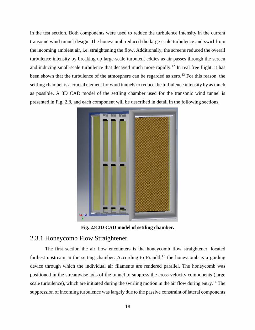
honeycomb cell types used in wind tunnels are presented in Fig. 2.9. In general, the loss in a

honeycomb, defined by the pressure loss coefficient 𝐾ℎ, in a wind tunnel is usually less than 5%

of the total tunnel loss.20 The loss coefficient is the ratio of pressure loss of the honeycomb to the

dynamic pressure at the entrance of the honeycomb.16 For the circular, square, and hexagonal

honeycombs presented in Fig. 2.9, the pressure loss coefficients for an L/D=6 are 0.3, 0.22, and

0.2 respectively.20 The hexagonal honeycomb type was selected for the transonic wind tunnel

because it had the lowest pressure loss coefficient and therefore was the most efficient for wind

tunnel turbulence reduction.

Fig. 2.9 a) Circular honeycomb; b) square honeycomb; c) hexagonal honeycomb.20

Typical L/D ratios for honeycombs range from 6-12, with 6-8 being the classical design20

and 8-12 have been used in more recent designs.14 The instability from the shear layer created in

the honeycomb is proportional to the shear layer thickness, therefore, a short honeycomb was

desired.15 In a recent study by Kulkarni et al.14, a series of computational fluid dynamics (CFD)

simulations were performed to find the optimal honeycomb-screen combination for wind tunnel

turbulence reduction. It was found that the optimal design was a honeycomb with L/D ratio in

between 8-10, followed by three screens downstream in the settling chamber. An adequate number

a) b) c)

20

of cells for a honeycomb is typically about 150 honeycomb cells per settling chamber hydraulic

diameter.17 The hydraulic diameter of the inlet was calculated using,

(2.10)

where 𝑎 is the height of the inlet, 47.522 inches, and 𝑏 is the width of the inlet, 31.681 inches.

Therefore, the hydraulic diameter of the inlet was 𝐷𝐻 = 38.017 inches. A cell diameter of 1/4

inches was chosen, as the cells per hydraulic diameter for this honeycomb size was equal to 152.

Once the cell diameter was selected, the L/D was determined by the available honeycomb core

stock material. The honeycomb was purchased from Universal Metaltek with the following

specifications: aluminum, 2.36 inch thickness, 1/4 inch cell diameter, 0.002 inch foil wall

thickness, and sheet size matching the height and width of the inlet. The 2.36 inch thickness

corresponded to an L/D=9.44, which was within the optimal range provided from the CFD study.14

2.3.2 Turbulence-Reducing Screens

The screens placed aft of the honeycomb were the components that actually reduced the

overall turbulence intensity. The screens improve the flow quality in terms of both velocity

uniformity and flow angularity.10 The resistance of a screen is proportional to the density of the

air and the square of the speed.12 The resistance per unit area can be calculated using,

(2.11)

where 𝑘 is the pressure-drop coefficient, 𝜌 is the air density, and 𝑈 is the mean velocity in the

settling chamber cross section. Since the velocity inside the settling chamber was relatively small

due to the high CR of the nozzle, the resistance of each screen was also small relative to the total

losses of the tunnel.

There were many configurations of screen size and spacing inside the settling chamber that

were considered when developing the transonic wind tunnel for this study. Based on CFD results

from Kulkarni et al.14 and other experiments11, the configuration of three screens aft of the

honeycomb section was selected for the wind tunnel. The selection of screen size was based on a

study performed by Derbunovich et al.11, in which the optimum arrangement of turbulence screens

were investigated. The screen configurations investigated are presented in Table 2.1, where 𝜀0𝑒𝑞

𝐷𝐻 =2𝑎𝑏

𝑎 + 𝑏

∆𝑝 = 𝑘 (1

2) 𝜌𝑈2

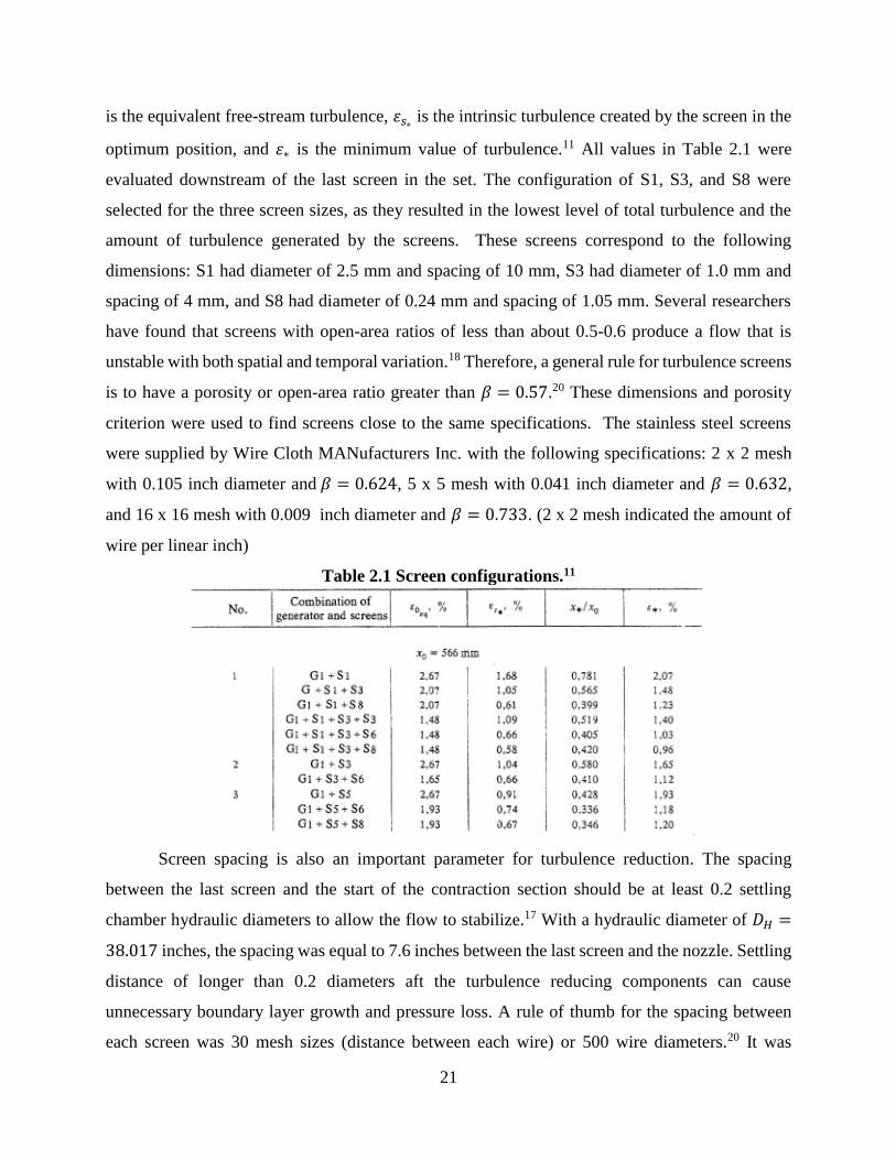
21

is the equivalent free-stream turbulence, 𝜀𝑠∗ is the intrinsic turbulence created by the screen in the

optimum position, and 𝜀∗ is the minimum value of turbulence.11 All values in Table 2.1 were

evaluated downstream of the last screen in the set. The configuration of S1, S3, and S8 were

selected for the three screen sizes, as they resulted in the lowest level of total turbulence and the

amount of turbulence generated by the screens. These screens correspond to the following

dimensions: S1 had diameter of 2.5 mm and spacing of 10 mm, S3 had diameter of 1.0 mm and

spacing of 4 mm, and S8 had diameter of 0.24 mm and spacing of 1.05 mm. Several researchers

have found that screens with open-area ratios of less than about 0.5-0.6 produce a flow that is

unstable with both spatial and temporal variation.18 Therefore, a general rule for turbulence screens

is to have a porosity or open-area ratio greater than 𝛽 = 0.57.20 These dimensions and porosity

criterion were used to find screens close to the same specifications. The stainless steel screens

were supplied by Wire Cloth MANufacturers Inc. with the following specifications: 2 x 2 mesh

with 0.105 inch diameter and 𝛽 = 0.624, 5 x 5 mesh with 0.041 inch diameter and 𝛽 = 0.632,

and 16 x 16 mesh with 0.009 inch diameter and 𝛽 = 0.733. (2 x 2 mesh indicated the amount of

wire per linear inch)

Table 2.1 Screen configurations.11

Screen spacing is also an important parameter for turbulence reduction. The spacing

between the last screen and the start of the contraction section should be at least 0.2 settling

chamber hydraulic diameters to allow the flow to stabilize.17 With a hydraulic diameter of 𝐷𝐻 =

38.017 inches, the spacing was equal to 7.6 inches between the last screen and the nozzle. Settling

distance of longer than 0.2 diameters aft the turbulence reducing components can cause

unnecessary boundary layer growth and pressure loss. A rule of thumb for the spacing between

each screen was 30 mesh sizes (distance between each wire) or 500 wire diameters.20 It was

22

estimated that the turbulence created by each screen persists for at least 200 screen mesh lengths.18

Using this criteria, the screens were spaced 5 inches apart from each preceding screen and the first

screen was placed 5 inches from the exit of the honeycomb. The total length of the settling chamber

was 25 inches after installation of honeycomb, three screens, and adequate spacing.

2.3.3 Settling Chamber Manufacturing

The settling chamber was manufactured by the UIUC Aerospace Engineering Machine

Shop and myself. The walls of the settling chamber were made of 1/4 inch thick aluminum 6061

flat bar. Each piece was machined into a panel that served as a track system for the screen and

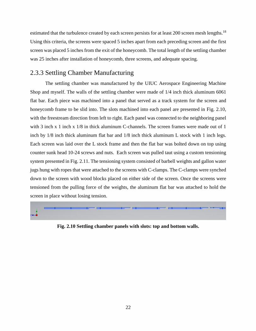
honeycomb frame to be slid into. The slots machined into each panel are presented in Fig. 2.10,

with the freestream direction from left to right. Each panel was connected to the neighboring panel

with 3 inch x 1 inch x 1/8 in thick aluminum C-channels. The screen frames were made out of 1

inch by 1/8 inch thick aluminum flat bar and 1/8 inch thick aluminum L stock with 1 inch legs.

Each screen was laid over the L stock frame and then the flat bar was bolted down on top using

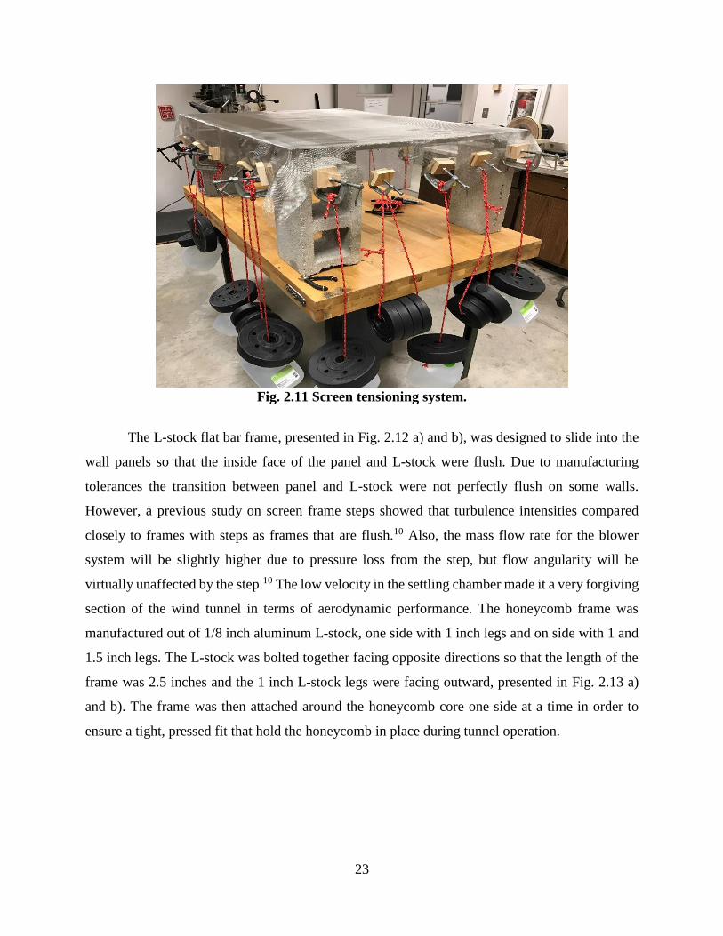
counter sunk head 10-24 screws and nuts. Each screen was pulled taut using a custom tensioning

system presented in Fig. 2.11. The tensioning system consisted of barbell weights and gallon water

jugs hung with ropes that were attached to the screens with C-clamps. The C-clamps were synched

down to the screen with wood blocks placed on either side of the screen. Once the screens were

tensioned from the pulling force of the weights, the aluminum flat bar was attached to hold the

screen in place without losing tension.

Fig. 2.10 Settling chamber panels with slots: top and bottom walls.

23

Fig. 2.11 Screen tensioning system.

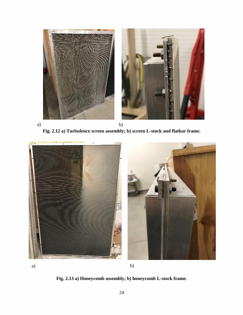
The L-stock flat bar frame, presented in Fig. 2.12 a) and b), was designed to slide into the

wall panels so that the inside face of the panel and L-stock were flush. Due to manufacturing

tolerances the transition between panel and L-stock were not perfectly flush on some walls.

However, a previous study on screen frame steps showed that turbulence intensities compared

closely to frames with steps as frames that are flush.10 Also, the mass flow rate for the blower

system will be slightly higher due to pressure loss from the step, but flow angularity will be

virtually unaffected by the step.10 The low velocity in the settling chamber made it a very forgiving

section of the wind tunnel in terms of aerodynamic performance. The honeycomb frame was

manufactured out of 1/8 inch aluminum L-stock, one side with 1 inch legs and on side with 1 and

1.5 inch legs. The L-stock was bolted together facing opposite directions so that the length of the

frame was 2.5 inches and the 1 inch L-stock legs were facing outward, presented in Fig. 2.13 a)

and b). The frame was then attached around the honeycomb core one side at a time in order to

ensure a tight, pressed fit that hold the honeycomb in place during tunnel operation.

24

Fig. 2.12 a) Turbulence screen assembly; b) screen L-stock and flatbar frame.

Fig. 2.13 a) Honeycomb assembly; b) honeycomb L-stock frame.

a) b)

a) b)

25

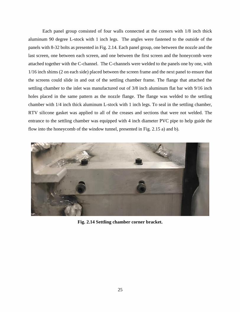
Each panel group consisted of four walls connected at the corners with 1/8 inch thick

aluminum 90 degree L-stock with 1 inch legs. The angles were fastened to the outside of the

panels with 8-32 bolts as presented in Fig. 2.14. Each panel group, one between the nozzle and the

last screen, one between each screen, and one between the first screen and the honeycomb were

attached together with the C-channel. The C-channels were welded to the panels one by one, with

1/16 inch shims (2 on each side) placed between the screen frame and the next panel to ensure that

the screens could slide in and out of the settling chamber frame. The flange that attached the

settling chamber to the inlet was manufactured out of 3/8 inch aluminum flat bar with 9/16 inch

holes placed in the same pattern as the nozzle flange. The flange was welded to the settling

chamber with 1/4 inch thick aluminum L-stock with 1 inch legs. To seal in the settling chamber,

RTV silicone gasket was applied to all of the creases and sections that were not welded. The

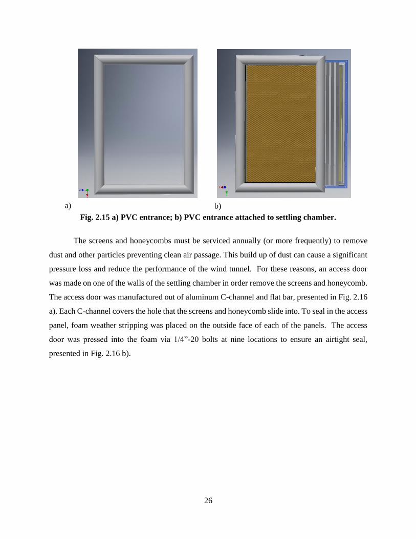
entrance to the settling chamber was equipped with 4 inch diameter PVC pipe to help guide the

flow into the honeycomb of the window tunnel, presented in Fig. 2.15 a) and b).

Fig. 2.14 Settling chamber corner bracket.

26

Fig. 2.15 a) PVC entrance; b) PVC entrance attached to settling chamber.

The screens and honeycombs must be serviced annually (or more frequently) to remove

dust and other particles preventing clean air passage. This build up of dust can cause a significant

pressure loss and reduce the performance of the wind tunnel. For these reasons, an access door

was made on one of the walls of the settling chamber in order remove the screens and honeycomb.

The access door was manufactured out of aluminum C-channel and flat bar, presented in Fig. 2.16

a). Each C-channel covers the hole that the screens and honeycomb slide into. To seal in the access

panel, foam weather stripping was placed on the outside face of each of the panels. The access

door was pressed into the foam via 1/4”-20 bolts at nine locations to ensure an airtight seal,

presented in Fig. 2.16 b).

a) b)

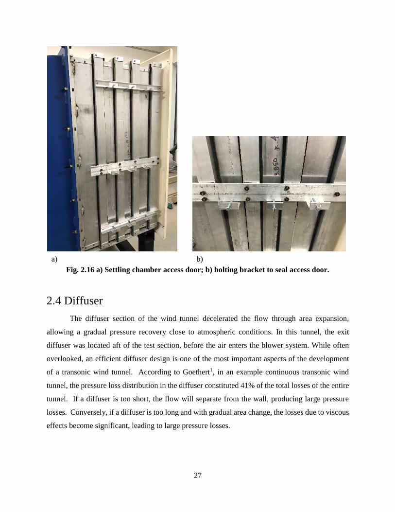
27

Fig. 2.16 a) Settling chamber access door; b) bolting bracket to seal access door.

2.4 Diffuser

The diffuser section of the wind tunnel decelerated the flow through area expansion,

allowing a gradual pressure recovery close to atmospheric conditions. In this tunnel, the exit

diffuser was located aft of the test section, before the air enters the blower system. While often

overlooked, an efficient diffuser design is one of the most important aspects of the development

of a transonic wind tunnel. According to Goethert1, in an example continuous transonic wind

tunnel, the pressure loss distribution in the diffuser constituted 41% of the total losses of the entire

tunnel. If a diffuser is too short, the flow will separate from the wall, producing large pressure

losses. Conversely, if a diffuser is too long and with gradual area change, the losses due to viscous

effects become significant, leading to large pressure losses.

a) b)

28

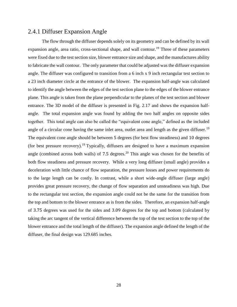
2.4.1 Diffuser Expansion Angle

The flow through the diffuser depends solely on its geometry and can be defined by its wall

expansion angle, area ratio, cross-sectional shape, and wall contour.19 Three of these parameters

were fixed due to the test section size, blower entrance size and shape, and the manufactures ability

to fabricate the wall contour. The only parameter that could be adjusted was the diffuser expansion

angle. The diffuser was configured to transition from a 6 inch x 9 inch rectangular test section to

a 23 inch diameter circle at the entrance of the blower. The expansion half-angle was calculated

to identify the angle between the edges of the test section plane to the edges of the blower entrance

plane. This angle is taken from the plane perpendicular to the planes of the test section and blower

entrance. The 3D model of the diffuser is presented in Fig. 2.17 and shows the expansion half-

angle. The total expansion angle was found by adding the two half angles on opposite sides

together. This total angle can also be called the “equivalent cone angle,” defined as the included

angle of a circular cone having the same inlet area, outlet area and length as the given diffuser.19

The equivalent cone angle should be between 5 degrees (for best flow steadiness) and 10 degrees

(for best pressure recovery).19 Typically, diffusers are designed to have a maximum expansion

angle (combined across both walls) of 7.5 degrees.20 This angle was chosen for the benefits of

both flow steadiness and pressure recovery. While a very long diffuser (small angle) provides a

deceleration with little chance of flow separation, the pressure losses and power requirements do

to the large length can be costly. In contrast, while a short wide-angle diffuser (large angle)

provides great pressure recovery, the change of flow separation and unsteadiness was high. Due

to the rectangular test section, the expansion angle could not be the same for the transition from

the top and bottom to the blower entrance as is from the sides. Therefore, an expansion half-angle

of 3.75 degrees was used for the sides and 3.09 degrees for the top and bottom (calculated by

taking the arc tangent of the vertical difference between the top of the test section to the top of the

blower entrance and the total length of the diffuser). The expansion angle defined the length of the

diffuser, the final design was 129.685 inches.

29

Fig. 2.17 a) Diffuser side view; b) diffuser isometric view.

The velocity at the exit of the diffuser was calculated from the area of the exit plane and

mass flow rate for operating conditions. Dividing the mass flow rate by the area and converting

units gives a velocity of 125 ft/s and a Mach number of M=0.11. Therefore, it can be stated that

the diffuser decelerates the flow to an adequate velocity for the blower system volumetric flow

rate of 21,500 CFM.

2.4.2 Diffuser Material and Manufacturing

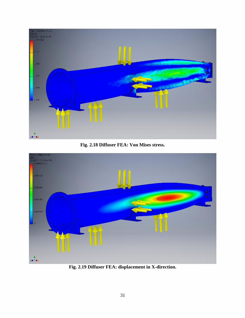
The diffuser and nozzle were manufactured from 3/8 inch thick steel. A finite element

analysis (FEA), presented in Fig. 2.18 and Fig. 2.19, was performed based on the pressure

differential in the diffuser and the ambient laboratory conditions. The static pressure inside the

wind tunnel will be lower than the atmospheric pressure outside the tunnel due to the increase in

dynamic pressure inside the tunnel. The FEA was performed for the largest pressure differential

when the test section Mach number is at the maximum of M=0.8. Since the outside of the tunnel

a)

b)

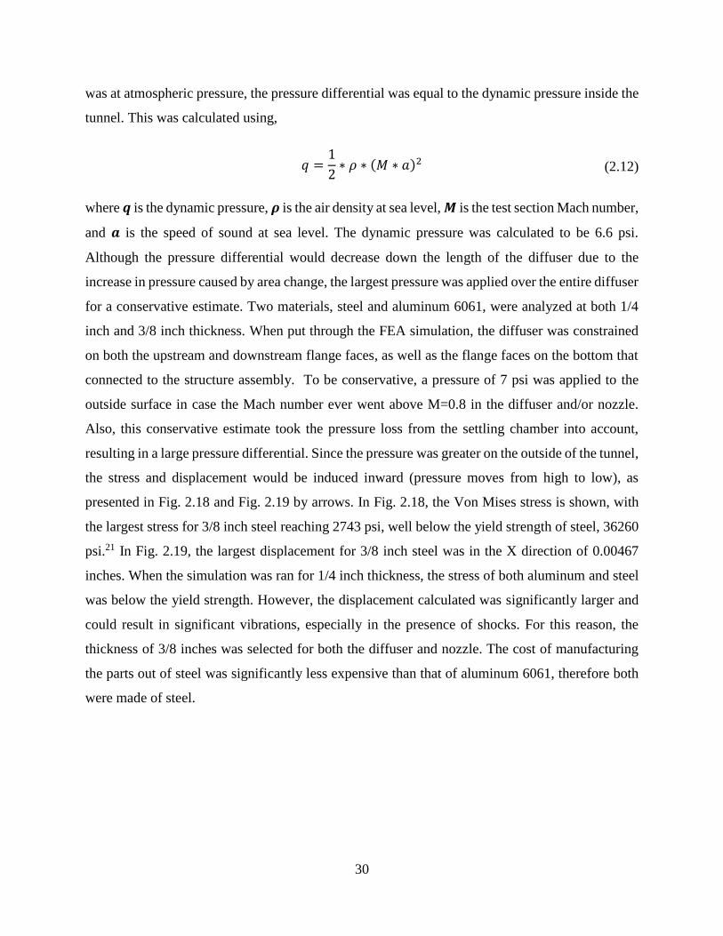
30

was at atmospheric pressure, the pressure differential was equal to the dynamic pressure inside the

tunnel. This was calculated using,

(2.12)

where 𝒒 is the dynamic pressure, 𝝆 is the air density at sea level, 𝑴 is the test section Mach number,

and 𝒂 is the speed of sound at sea level. The dynamic pressure was calculated to be 6.6 psi.

Although the pressure differential would decrease down the length of the diffuser due to the

increase in pressure caused by area change, the largest pressure was applied over the entire diffuser

for a conservative estimate. Two materials, steel and aluminum 6061, were analyzed at both 1/4

inch and 3/8 inch thickness. When put through the FEA simulation, the diffuser was constrained

on both the upstream and downstream flange faces, as well as the flange faces on the bottom that

connected to the structure assembly. To be conservative, a pressure of 7 psi was applied to the

outside surface in case the Mach number ever went above M=0.8 in the diffuser and/or nozzle.

Also, this conservative estimate took the pressure loss from the settling chamber into account,

resulting in a large pressure differential. Since the pressure was greater on the outside of the tunnel,

the stress and displacement would be induced inward (pressure moves from high to low), as

presented in Fig. 2.18 and Fig. 2.19 by arrows. In Fig. 2.18, the Von Mises stress is shown, with

the largest stress for 3/8 inch steel reaching 2743 psi, well below the yield strength of steel, 36260

psi.21 In Fig. 2.19, the largest displacement for 3/8 inch steel was in the X direction of 0.00467

inches. When the simulation was ran for 1/4 inch thickness, the stress of both aluminum and steel

was below the yield strength. However, the displacement calculated was significantly larger and

could result in significant vibrations, especially in the presence of shocks. For this reason, the

thickness of 3/8 inches was selected for both the diffuser and nozzle. The cost of manufacturing

the parts out of steel was significantly less expensive than that of aluminum 6061, therefore both

were made of steel.

𝑞 =1

2∗ 𝜌 ∗ (𝑀 ∗ 𝑎)2

31

Fig. 2.18 Diffuser FEA: Von Mises stress.

Fig. 2.19 Diffuser FEA: displacement in X-direction.

32

The nozzle and diffuser were manufactured by Fox Valley Metal Tech by bending and

shaping the parts to the specified dimensions. The parts were welded together after each panel was

formed. As an added measure of safety, a sheet of metal twisted-wire fencing was installed

between the downstream end of the diffuser and the blower entrance flanges. The hexagonal

openings were 1 in (height) by 1.5 in (width) with a wire diameter of 0.035 inches. The fencing

will stop any large objects that may come down the tunnel from hitting and possibly damaging the

blades of the fan. The horizontal flanges were 1/2 inch thick and connected to the structural

assembly with 1/2” -13 socket head bolts, washers, and nuts. The circular flange that connected

the diffuser to the blower was attached with 1/2”-13 socket head bolts, washers, and nuts.

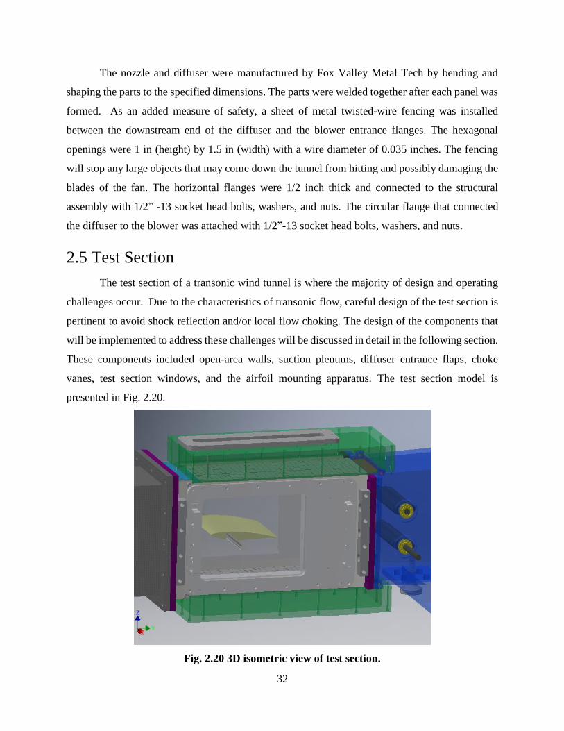
2.5 Test Section

The test section of a transonic wind tunnel is where the majority of design and operating

challenges occur. Due to the characteristics of transonic flow, careful design of the test section is

pertinent to avoid shock reflection and/or local flow choking. The design of the components that

will be implemented to address these challenges will be discussed in detail in the following section.

These components included open-area walls, suction plenums, diffuser entrance flaps, choke

vanes, test section windows, and the airfoil mounting apparatus. The test section model is

presented in Fig. 2.20.

Fig. 2.20 3D isometric view of test section.

33

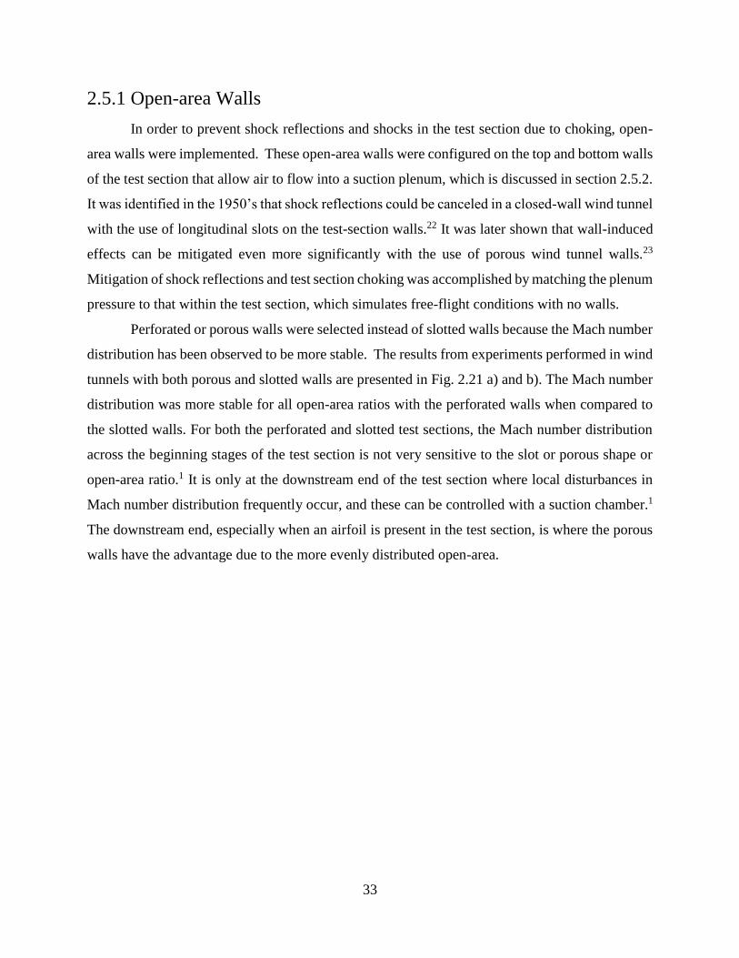
2.5.1 Open-area Walls

In order to prevent shock reflections and shocks in the test section due to choking, open-

area walls were implemented. These open-area walls were configured on the top and bottom walls

of the test section that allow air to flow into a suction plenum, which is discussed in section 2.5.2.

It was identified in the 1950’s that shock reflections could be canceled in a closed-wall wind tunnel

with the use of longitudinal slots on the test-section walls.22 It was later shown that wall-induced

effects can be mitigated even more significantly with the use of porous wind tunnel walls.23

Mitigation of shock reflections and test section choking was accomplished by matching the plenum

pressure to that within the test section, which simulates free-flight conditions with no walls.

Perforated or porous walls were selected instead of slotted walls because the Mach number

distribution has been observed to be more stable. The results from experiments performed in wind

tunnels with both porous and slotted walls are presented in Fig. 2.21 a) and b). The Mach number

distribution was more stable for all open-area ratios with the perforated walls when compared to

the slotted walls. For both the perforated and slotted test sections, the Mach number distribution

across the beginning stages of the test section is not very sensitive to the slot or porous shape or

open-area ratio.1 It is only at the downstream end of the test section where local disturbances in

Mach number distribution frequently occur, and these can be controlled with a suction chamber.1

The downstream end, especially when an airfoil is present in the test section, is where the porous

walls have the advantage due to the more evenly distributed open-area.

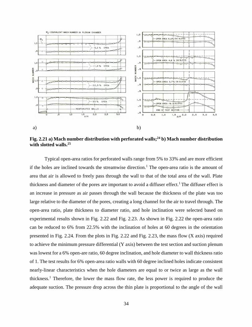
34

Fig. 2.21 a) Mach number distribution with perforated walls;24 b) Mach number distribution

with slotted walls.25

Typical open-area ratios for perforated walls range from 5% to 33% and are more efficient

if the holes are inclined towards the streamwise direction.1 The open-area ratio is the amount of

area that air is allowed to freely pass through the wall to that of the total area of the wall. Plate

thickness and diameter of the pores are important to avoid a diffuser effect.1 The diffuser effect is

an increase in pressure as air passes through the wall because the thickness of the plate was too

large relative to the diameter of the pores, creating a long channel for the air to travel through. The

open-area ratio, plate thickness to diameter ratio, and hole inclination were selected based on

experimental results shown in Fig. 2.22 and Fig. 2.23. As shown in Fig. 2.22 the open-area ratio

can be reduced to 6% from 22.5% with the inclination of holes at 60 degrees in the orientation

presented in Fig. 2.24. From the plots in Fig. 2.22 and Fig. 2.23, the mass flow (X axis) required

to achieve the minimum pressure differential (Y axis) between the test section and suction plenum

was lowest for a 6% open-are ratio, 60 degree inclination, and hole diameter to wall thickness ratio

of 1. The test results for 6% open-area ratio walls with 60 degree inclined holes indicate consistent

nearly-linear characteristics when the hole diameters are equal to or twice as large as the wall

thickness.1 Therefore, the lower the mass flow rate, the less power is required to produce the

adequate suction. The pressure drop across the thin plate is proportional to the angle of the wall

a) b)

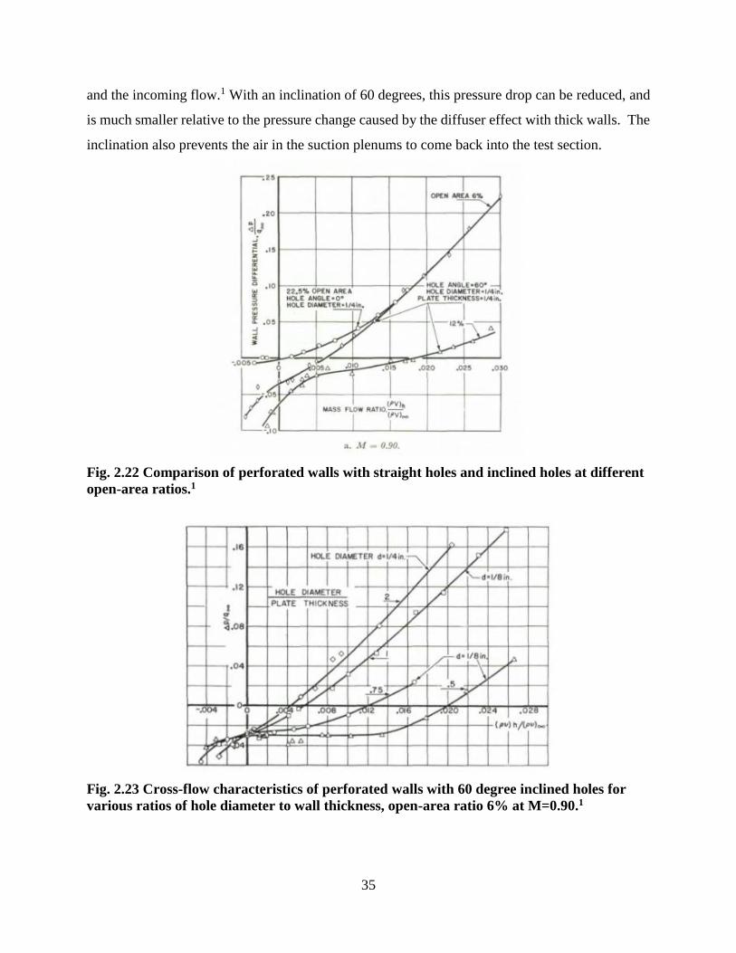
35

and the incoming flow.1 With an inclination of 60 degrees, this pressure drop can be reduced, and

is much smaller relative to the pressure change caused by the diffuser effect with thick walls. The

inclination also prevents the air in the suction plenums to come back into the test section.

Fig. 2.22 Comparison of perforated walls with straight holes and inclined holes at different

open-area ratios.1

Fig. 2.23 Cross-flow characteristics of perforated walls with 60 degree inclined holes for

various ratios of hole diameter to wall thickness, open-area ratio 6% at M=0.90.1

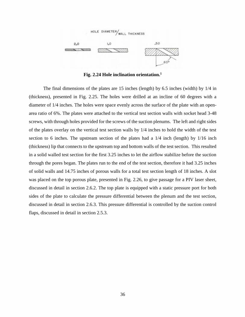
36

Fig. 2.24 Hole inclination orientation.1

The final dimensions of the plates are 15 inches (length) by 6.5 inches (width) by 1/4 in

(thickness), presented in Fig. 2.25. The holes were drilled at an incline of 60 degrees with a

diameter of 1/4 inches. The holes were space evenly across the surface of the plate with an open-

area ratio of 6%. The plates were attached to the vertical test section walls with socket head 3-48

screws, with through holes provided for the screws of the suction plenums. The left and right sides

of the plates overlay on the vertical test section walls by 1/4 inches to hold the width of the test

section to 6 inches. The upstream section of the plates had a 1/4 inch (length) by 1/16 inch

(thickness) lip that connects to the upstream top and bottom walls of the test section. This resulted

in a solid walled test section for the first 3.25 inches to let the airflow stabilize before the suction

through the pores began. The plates run to the end of the test section, therefore it had 3.25 inches

of solid walls and 14.75 inches of porous walls for a total test section length of 18 inches. A slot

was placed on the top porous plate, presented in Fig. 2.26, to give passage for a PIV laser sheet,

discussed in detail in section 2.6.2. The top plate is equipped with a static pressure port for both

sides of the plate to calculate the pressure differential between the plenum and the test section,

discussed in detail in section 2.6.3. This pressure differential is controlled by the suction control

flaps, discussed in detail in section 2.5.3.

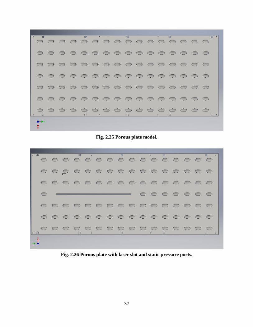
37

Fig. 2.25 Porous plate model.

Fig. 2.26 Porous plate with laser slot and static pressure ports.

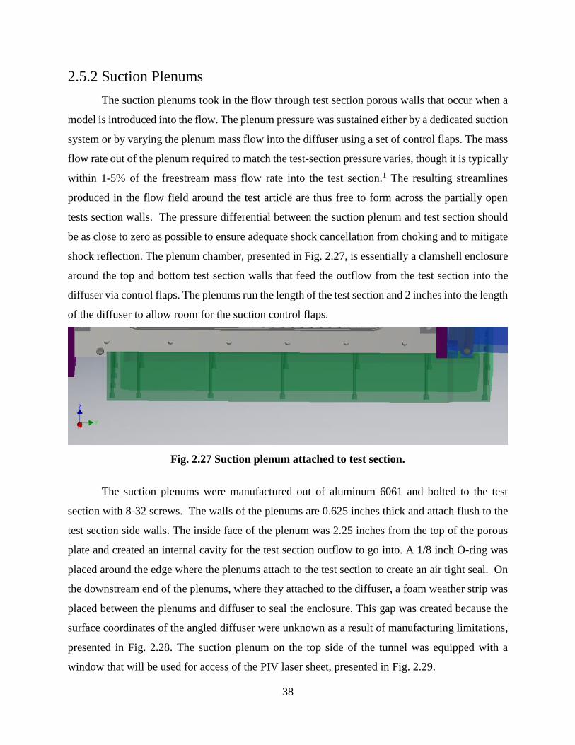
38

2.5.2 Suction Plenums

The suction plenums took in the flow through test section porous walls that occur when a

model is introduced into the flow. The plenum pressure was sustained either by a dedicated suction

system or by varying the plenum mass flow into the diffuser using a set of control flaps. The mass

flow rate out of the plenum required to match the test-section pressure varies, though it is typically

within 1-5% of the freestream mass flow rate into the test section.1 The resulting streamlines

produced in the flow field around the test article are thus free to form across the partially open

tests section walls. The pressure differential between the suction plenum and test section should

be as close to zero as possible to ensure adequate shock cancellation from choking and to mitigate

shock reflection. The plenum chamber, presented in Fig. 2.27, is essentially a clamshell enclosure

around the top and bottom test section walls that feed the outflow from the test section into the

diffuser via control flaps. The plenums run the length of the test section and 2 inches into the length

of the diffuser to allow room for the suction control flaps.

Fig. 2.27 Suction plenum attached to test section.

The suction plenums were manufactured out of aluminum 6061 and bolted to the test

section with 8-32 screws. The walls of the plenums are 0.625 inches thick and attach flush to the

test section side walls. The inside face of the plenum was 2.25 inches from the top of the porous

plate and created an internal cavity for the test section outflow to go into. A 1/8 inch O-ring was

placed around the edge where the plenums attach to the test section to create an air tight seal. On

the downstream end of the plenums, where they attached to the diffuser, a foam weather strip was

placed between the plenums and diffuser to seal the enclosure. This gap was created because the

surface coordinates of the angled diffuser were unknown as a result of manufacturing limitations,

presented in Fig. 2.28. The suction plenum on the top side of the tunnel was equipped with a

window that will be used for access of the PIV laser sheet, presented in Fig. 2.29.

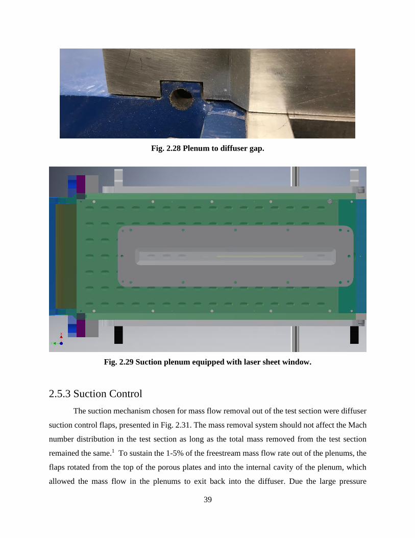
39

Fig. 2.28 Plenum to diffuser gap.

Fig. 2.29 Suction plenum equipped with laser sheet window.

2.5.3 Suction Control

The suction mechanism chosen for mass flow removal out of the test section were diffuser

suction control flaps, presented in Fig. 2.31. The mass removal system should not affect the Mach

number distribution in the test section as long as the total mass removed from the test section

remained the same.1 To sustain the 1-5% of the freestream mass flow rate out of the plenums, the

flaps rotated from the top of the porous plates and into the internal cavity of the plenum, which

allowed the mass flow in the plenums to exit back into the diffuser. Due the large pressure

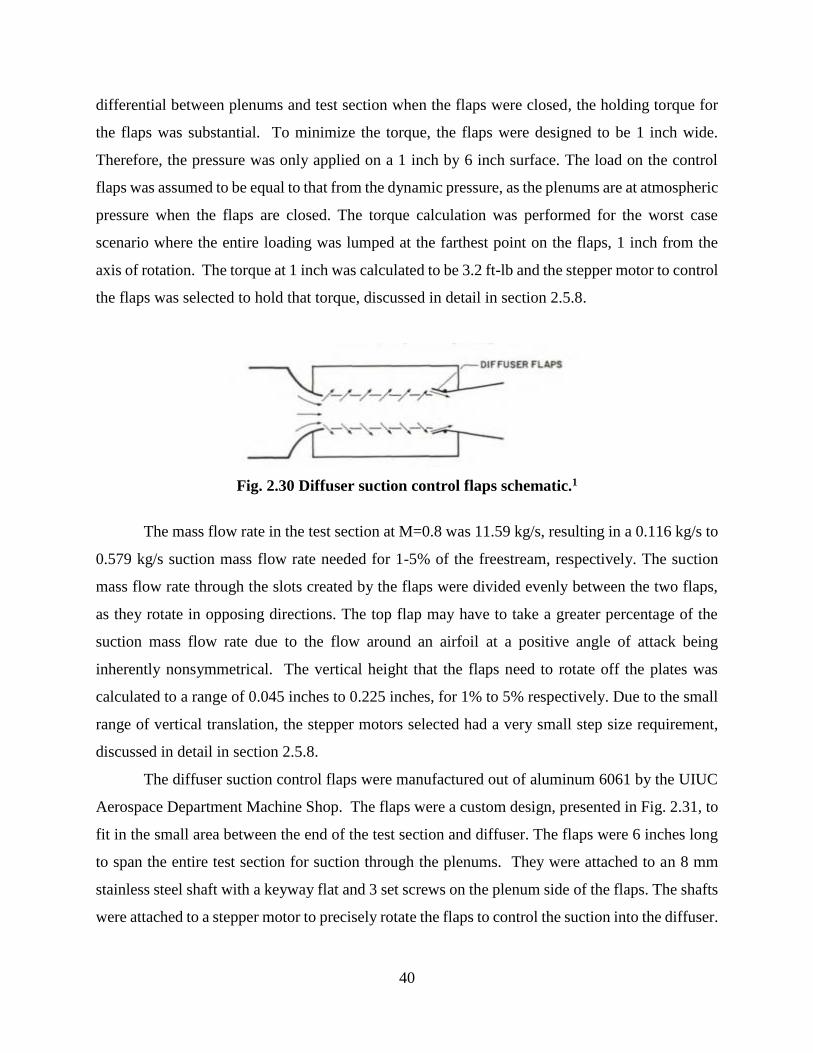
40

differential between plenums and test section when the flaps were closed, the holding torque for

the flaps was substantial. To minimize the torque, the flaps were designed to be 1 inch wide.

Therefore, the pressure was only applied on a 1 inch by 6 inch surface. The load on the control

flaps was assumed to be equal to that from the dynamic pressure, as the plenums are at atmospheric

pressure when the flaps are closed. The torque calculation was performed for the worst case

scenario where the entire loading was lumped at the farthest point on the flaps, 1 inch from the

axis of rotation. The torque at 1 inch was calculated to be 3.2 ft-lb and the stepper motor to control

the flaps was selected to hold that torque, discussed in detail in section 2.5.8.

Fig. 2.30 Diffuser suction control flaps schematic.1

The mass flow rate in the test section at M=0.8 was 11.59 kg/s, resulting in a 0.116 kg/s to

0.579 kg/s suction mass flow rate needed for 1-5% of the freestream, respectively. The suction

mass flow rate through the slots created by the flaps were divided evenly between the two flaps,

as they rotate in opposing directions. The top flap may have to take a greater percentage of the

suction mass flow rate due to the flow around an airfoil at a positive angle of attack being

inherently nonsymmetrical. The vertical height that the flaps need to rotate off the plates was

calculated to a range of 0.045 inches to 0.225 inches, for 1% to 5% respectively. Due to the small

range of vertical translation, the stepper motors selected had a very small step size requirement,

discussed in detail in section 2.5.8.

The diffuser suction control flaps were manufactured out of aluminum 6061 by the UIUC

Aerospace Department Machine Shop. The flaps were a custom design, presented in Fig. 2.31, to

fit in the small area between the end of the test section and diffuser. The flaps were 6 inches long

to span the entire test section for suction through the plenums. They were attached to an 8 mm

stainless steel shaft with a keyway flat and 3 set screws on the plenum side of the flaps. The shafts

were attached to a stepper motor to precisely rotate the flaps to control the suction into the diffuser.

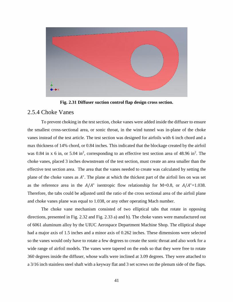
41

Fig. 2.31 Diffuser suction control flap design cross section.

2.5.4 Choke Vanes

To prevent choking in the test section, choke vanes were added inside the diffuser to ensure

the smallest cross-sectional area, or sonic throat, in the wind tunnel was in-plane of the choke

vanes instead of the test article. The test section was designed for airfoils with 6 inch chord and a

max thickness of 14% chord, or 0.84 inches. This indicated that the blockage created by the airfoil

was 0.84 in x 6 in, or 5.04 in2, corresponding to an effective test section area of 48.96 in2. The

choke vanes, placed 3 inches downstream of the test section, must create an area smaller than the

effective test section area. The area that the vanes needed to create was calculated by setting the

plane of the choke vanes as 𝐴∗. The plane at which the thickest part of the airfoil lies on was set

as the reference area in the 𝐴/𝐴∗ isentropic flow relationship for M=0.8, or 𝐴/𝐴∗=1.038.

Therefore, the tabs could be adjusted until the ratio of the cross sectional area of the airfoil plane

and choke vanes plane was equal to 1.038, or any other operating Mach number.

The choke vane mechanism consisted of two elliptical tabs that rotate in opposing

directions, presented in Fig. 2.32 and Fig. 2.33 a) and b). The choke vanes were manufactured out

of 6061 aluminum alloy by the UIUC Aerospace Department Machine Shop. The elliptical shape

had a major axis of 1.5 inches and a minor axis of 0.262 inches. These dimensions were selected

so the vanes would only have to rotate a few degrees to create the sonic throat and also work for a

wide range of airfoil models. The vanes were tapered on the ends so that they were free to rotate

360 degrees inside the diffuser, whose walls were inclined at 3.09 degrees. They were attached to

a 3/16 inch stainless steel shaft with a keyway flat and 3 set screws on the plenum side of the flaps.

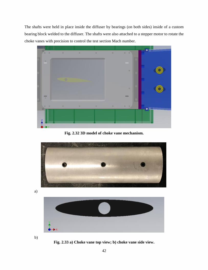
42

The shafts were held in place inside the diffuser by bearings (on both sides) inside of a custom

bearing block welded to the diffuser. The shafts were also attached to a stepper motor to rotate the

choke vanes with precision to control the test section Mach number.

Fig. 2.32 3D model of choke vane mechanism.

Fig. 2.33 a) Choke vane top view; b) choke vane side view.

a)

b)

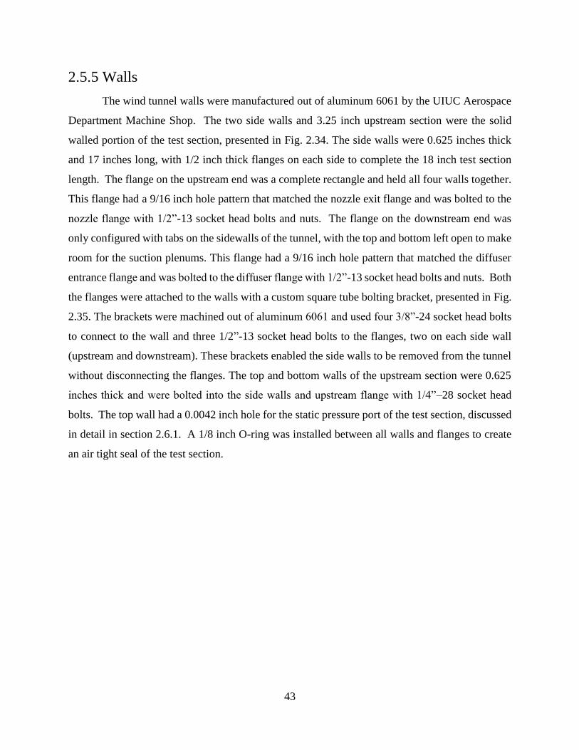
43

2.5.5 Walls

The wind tunnel walls were manufactured out of aluminum 6061 by the UIUC Aerospace

Department Machine Shop. The two side walls and 3.25 inch upstream section were the solid

walled portion of the test section, presented in Fig. 2.34. The side walls were 0.625 inches thick

and 17 inches long, with 1/2 inch thick flanges on each side to complete the 18 inch test section

length. The flange on the upstream end was a complete rectangle and held all four walls together.

This flange had a 9/16 inch hole pattern that matched the nozzle exit flange and was bolted to the

nozzle flange with 1/2”-13 socket head bolts and nuts. The flange on the downstream end was

only configured with tabs on the sidewalls of the tunnel, with the top and bottom left open to make

room for the suction plenums. This flange had a 9/16 inch hole pattern that matched the diffuser

entrance flange and was bolted to the diffuser flange with 1/2”-13 socket head bolts and nuts. Both

the flanges were attached to the walls with a custom square tube bolting bracket, presented in Fig.

2.35. The brackets were machined out of aluminum 6061 and used four 3/8”-24 socket head bolts

to connect to the wall and three 1/2”-13 socket head bolts to the flanges, two on each side wall

(upstream and downstream). These brackets enabled the side walls to be removed from the tunnel

without disconnecting the flanges. The top and bottom walls of the upstream section were 0.625

inches thick and were bolted into the side walls and upstream flange with 1/4”–28 socket head

bolts. The top wall had a 0.0042 inch hole for the static pressure port of the test section, discussed

in detail in section 2.6.1. A 1/8 inch O-ring was installed between all walls and flanges to create

an air tight seal of the test section.

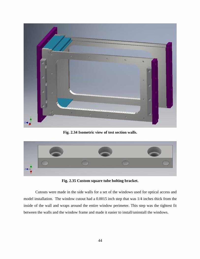
44

Fig. 2.34 Isometric view of test section walls.

Fig. 2.35 Custom square tube bolting bracket.

Cutouts were made in the side walls for a set of the windows used for optical access and

model installation. The window cutout had a 0.0015 inch step that was 1/4 inches thick from the

inside of the wall and wraps around the entire window perimeter. This step was the tightest fit

between the walls and the window frame and made it easier to install/uninstall the windows.

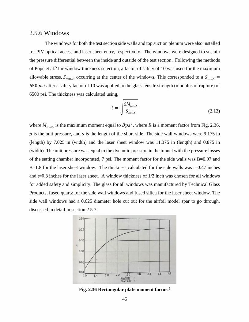
45

2.5.6 Windows

The windows for both the test section side walls and top suction plenum were also installed

for PIV optical access and laser sheet entry, respectively. The windows were designed to sustain

the pressure differential between the inside and outside of the test section. Following the methods

of Pope et al.5 for window thickness selection, a factor of safety of 10 was used for the maximum

allowable stress, 𝑆𝑚𝑎𝑥, occurring at the center of the windows. This corresponded to a 𝑆𝑚𝑎𝑥 =

650 𝑝𝑠𝑖 after a safety factor of 10 was applied to the glass tensile strength (modulus of rupture) of

6500 psi. The thickness was calculated using,

(2.13)

where 𝑀𝑚𝑎𝑥 is the maximum moment equal to 𝐵𝑝𝑠2, where 𝐵 is a moment factor from Fig. 2.36,

𝑝 is the unit pressure, and 𝑠 is the length of the short side. The side wall windows were 9.175 in

(length) by 7.025 in (width) and the laser sheet window was 11.375 in (length) and 0.875 in

(width). The unit pressure was equal to the dynamic pressure in the tunnel with the pressure losses

of the setting chamber incorporated, 7 psi. The moment factor for the side walls was B=0.07 and

B=1.8 for the laser sheet window. The thickness calculated for the side walls was t=0.47 inches

and t=0.3 inches for the laser sheet. A window thickness of 1/2 inch was chosen for all windows

for added safety and simplicity. The glass for all windows was manufactured by Technical Glass

Products, fused quartz for the side wall windows and fused silica for the laser sheet window. The

side wall windows had a 0.625 diameter hole cut out for the airfoil model spar to go through,

discussed in detail in section 2.5.7.

Fig. 2.36 Rectangular plate moment factor.5

𝑡 = √6𝑀𝑚𝑎𝑥

𝑆𝑚𝑎𝑥

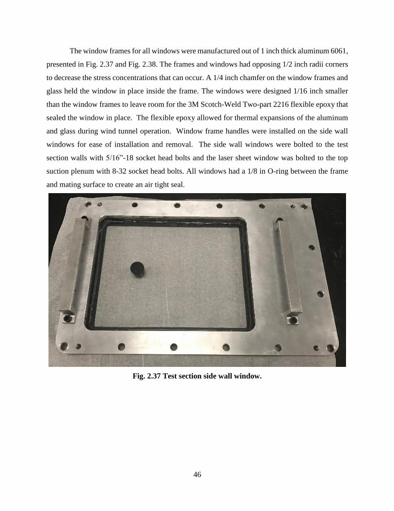
46

The window frames for all windows were manufactured out of 1 inch thick aluminum 6061,

presented in Fig. 2.37 and Fig. 2.38. The frames and windows had opposing 1/2 inch radii corners

to decrease the stress concentrations that can occur. A 1/4 inch chamfer on the window frames and

glass held the window in place inside the frame. The windows were designed 1/16 inch smaller

than the window frames to leave room for the 3M Scotch-Weld Two-part 2216 flexible epoxy that

sealed the window in place. The flexible epoxy allowed for thermal expansions of the aluminum

and glass during wind tunnel operation. Window frame handles were installed on the side wall

windows for ease of installation and removal. The side wall windows were bolted to the test

section walls with 5/16”-18 socket head bolts and the laser sheet window was bolted to the top

suction plenum with 8-32 socket head bolts. All windows had a 1/8 in O-ring between the frame

and mating surface to create an air tight seal.

Fig. 2.37 Test section side wall window.

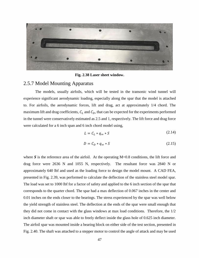
47

Fig. 2.38 Laser sheet window.

2.5.7 Model Mounting Apparatus

The models, usually airfoils, which will be tested in the transonic wind tunnel will

experience significant aerodynamic loading, especially along the spar that the model is attached

to. For airfoils, the aerodynamic forces, lift and drag, act at approximately 1/4 chord. The

maximum lift and drag coefficients, 𝐶𝐿 and 𝐶𝐷, that can be expected for the experiments performed

in the tunnel were conservatively estimated as 2.5 and 1, respectively. The lift force and drag force

were calculated for a 6 inch span and 6 inch chord model using,

(2.14)

(2.15)

where 𝑺 is the reference area of the airfoil. At the operating M=0.8 conditions, the lift force and

drag force were 2636 N and 1055 N, respectively. The resultant force was 2840 N or

approximately 640 lbf and used as the loading force to design the model mount. A CAD FEA,

presented in Fig. 2.39, was performed to calculate the deflection of the stainless steel model spar.

The load was set to 1000 lbf for a factor of safety and applied to the 6 inch section of the spar that

corresponds to the quarter chord. The spar had a max deflection of 0.067 inches in the center and

0.01 inches on the ends closer to the bearings. The stress experienced by the spar was well below

the yield strength of stainless steel. The deflection at the ends of the spar were small enough that

they did not come in contact with the glass windows at max load conditions. Therefore, the 1/2

inch diameter shaft or spar was able to freely deflect inside the glass hole of 0.625 inch diameter.

The airfoil spar was mounted inside a bearing block on either side of the test section, presented in

Fig. 2.40. The shaft was attached to a stepper motor to control the angle of attack and may be used

𝐿 = 𝐶𝐿 ∗ 𝑞∞ ∗ 𝑆

𝐷 = 𝐶𝐷 ∗ 𝑞∞ ∗ 𝑆

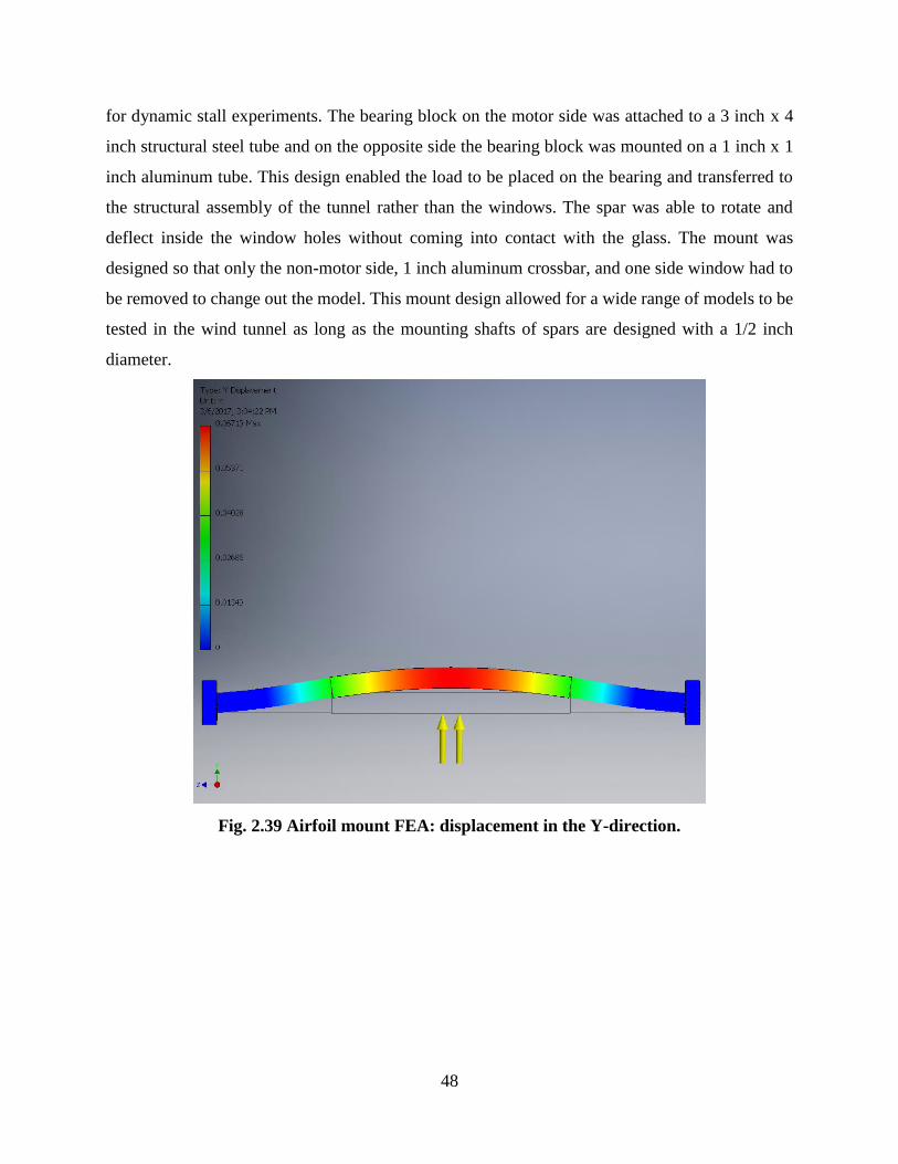
48

for dynamic stall experiments. The bearing block on the motor side was attached to a 3 inch x 4

inch structural steel tube and on the opposite side the bearing block was mounted on a 1 inch x 1

inch aluminum tube. This design enabled the load to be placed on the bearing and transferred to

the structural assembly of the tunnel rather than the windows. The spar was able to rotate and

deflect inside the window holes without coming into contact with the glass. The mount was

designed so that only the non-motor side, 1 inch aluminum crossbar, and one side window had to

be removed to change out the model. This mount design allowed for a wide range of models to be

tested in the wind tunnel as long as the mounting shafts of spars are designed with a 1/2 inch

diameter.

Fig. 2.39 Airfoil mount FEA: displacement in the Y-direction.

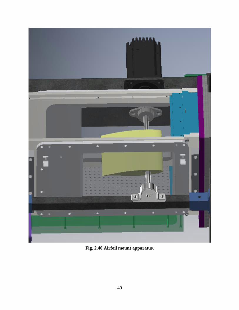
49

Fig. 2.40 Airfoil mount apparatus.

50

2.5.8 Stepper Motor Selection

A set of stepper motors for the wind tunnel were used for suction control, Mach number

calibration, and model adjustments such as angle of attack. The selection of the motors was based

on the holding torque and rotational step size required. The maximum holding torque will occur

during actuation of the diffuser suction control flaps. This torque was evaluated to be 3.2 ft-lb or

615 oz-in and was much greater than the torque experienced by the model mount system or choke

vanes. The stepper resolution was based on the precision required for the diffuser suction control

flaps. The vertical distance travelled by the flaps for a 1% to 5% freestream mass flow rate was

only 0.18 inches (maximum distance of 0.225 inches minus minimum distance of 0.045 inches).

This resulted in a 10.2 degree window of rotation for the flaps. The majority of stepper motors

researched had a 1.8 degree step resolution and did not provide the accuracy required for adequate

suction control (only 6 steps for the flaps). Therefore, the Anaheim Automation 34MDSI214S was

selected for all 5 stepper motors, one for each control flap, one for each choke vane, and one for

the model mount system. These motors had a 1200 oz-in holding torque and 0.225 degree

resolution with micro-stepping. The small step size allowed for 45 steps of precision for suction

control, as well as precise Mach number control with the choke vanes and model adjustments. To

simplify system integration, the same motor was used for all control applications, even if the torque

loads and step resolution required were less for that of the choke vanes and model mount system.

The motors were installed in line with each of the shafts for the control flaps, choke vanes, and

model using zero-backlash replaceable-center flexible shaft couplings.

2.6 Data Acquisition Capabilities

The transonic wind tunnel was designed to have the capability to perform multiple data

measurement methods. These include but are not limited to: Schlieren flow visualization, time

resolved PIV, stereoscopic PIV, static pressure measurement, wake rake pressure surveys, and

thermocouple temperature measurements.

2.6.1 Mach Number Control via Static Pressure Taps and Thermocouple

The Mach number in the test section, controlled via choke vanes, was defined as the driving

parameter of the wind tunnel. Static pressure taps in the settling chamber and test section, along

with a thermocouple outside the tunnel, are used to calculate the Mach number. A static pressure

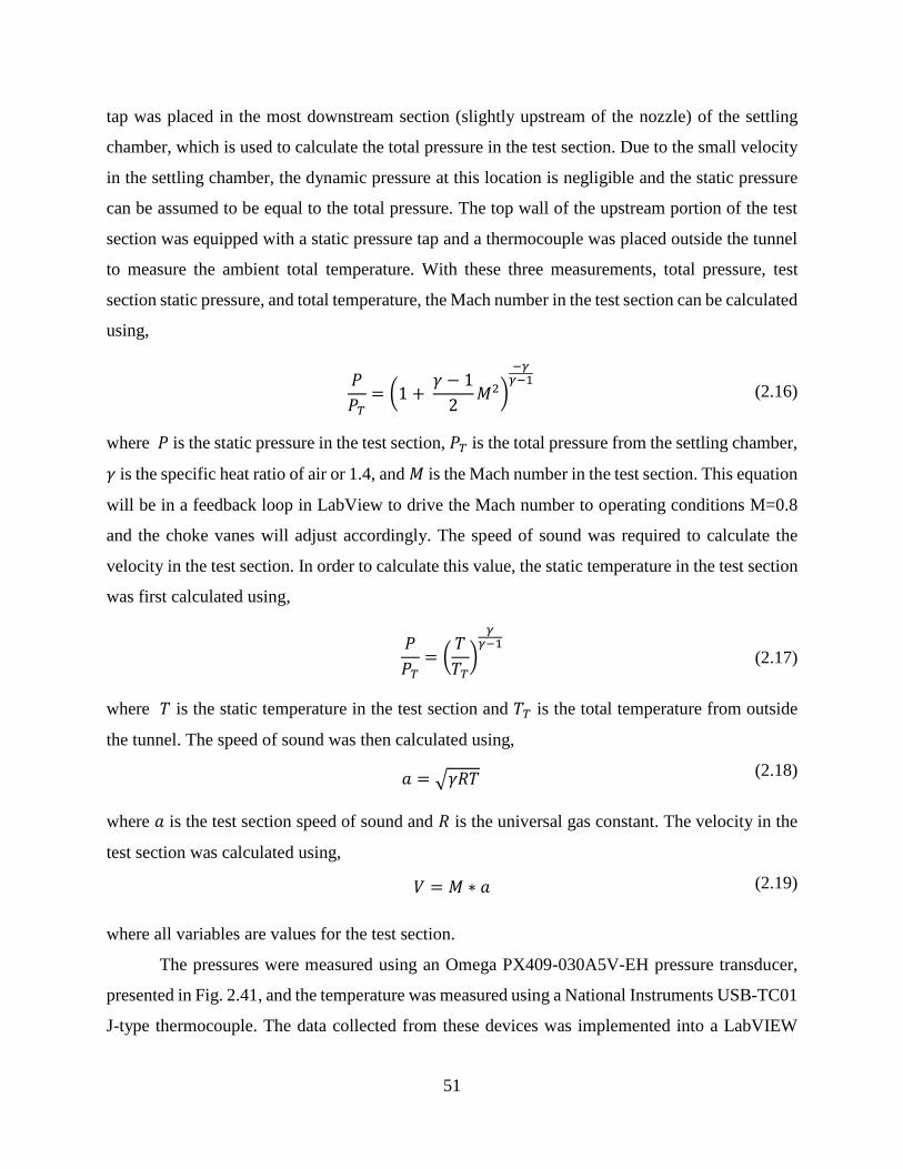
51

tap was placed in the most downstream section (slightly upstream of the nozzle) of the settling

chamber, which is used to calculate the total pressure in the test section. Due to the small velocity

in the settling chamber, the dynamic pressure at this location is negligible and the static pressure

can be assumed to be equal to the total pressure. The top wall of the upstream portion of the test

section was equipped with a static pressure tap and a thermocouple was placed outside the tunnel

to measure the ambient total temperature. With these three measurements, total pressure, test

section static pressure, and total temperature, the Mach number in the test section can be calculated

using,

(2.16)

where 𝑃 is the static pressure in the test section, 𝑃𝑇 is the total pressure from the settling chamber,

𝛾 is the specific heat ratio of air or 1.4, and 𝑀 is the Mach number in the test section. This equation

will be in a feedback loop in LabView to drive the Mach number to operating conditions M=0.8

and the choke vanes will adjust accordingly. The speed of sound was required to calculate the

velocity in the test section. In order to calculate this value, the static temperature in the test section

was first calculated using,

(2.17)

where 𝑇 is the static temperature in the test section and 𝑇𝑇 is the total temperature from outside

the tunnel. The speed of sound was then calculated using,

(2.18)

where 𝑎 is the test section speed of sound and 𝑅 is the universal gas constant. The velocity in the

test section was calculated using,

(2.19)

where all variables are values for the test section.

The pressures were measured using an Omega PX409-030A5V-EH pressure transducer,

presented in Fig. 2.41, and the temperature was measured using a National Instruments USB-TC01

J-type thermocouple. The data collected from these devices was implemented into a LabVIEW

𝑃

𝑃𝑇= (

𝑇

𝑇𝑇)

𝛾𝛾−1

𝑎 = √𝛾𝑅𝑇

𝑉 = 𝑀 ∗ 𝑎

𝑃

𝑃𝑇= (1 +

𝛾 − 1

2𝑀2)

−𝛾𝛾−1

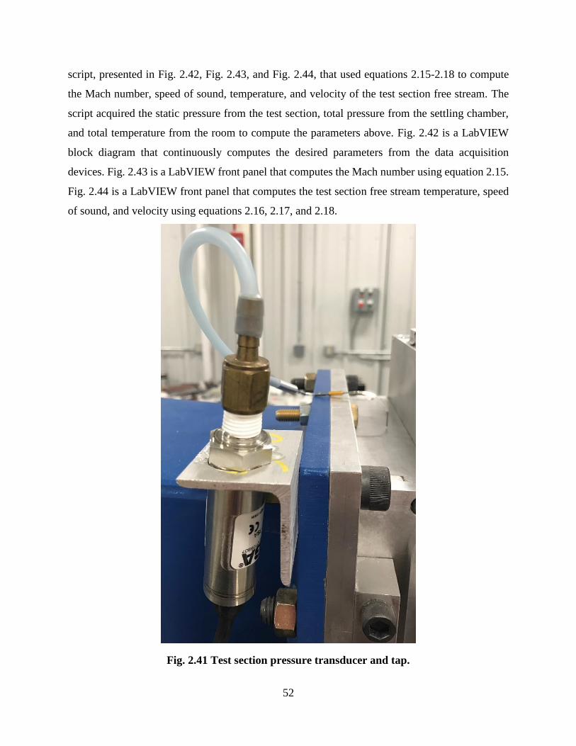
52

script, presented in Fig. 2.42, Fig. 2.43, and Fig. 2.44, that used equations 2.15-2.18 to compute

the Mach number, speed of sound, temperature, and velocity of the test section free stream. The

script acquired the static pressure from the test section, total pressure from the settling chamber,

and total temperature from the room to compute the parameters above. Fig. 2.42 is a LabVIEW

block diagram that continuously computes the desired parameters from the data acquisition

devices. Fig. 2.43 is a LabVIEW front panel that computes the Mach number using equation 2.15.

Fig. 2.44 is a LabVIEW front panel that computes the test section free stream temperature, speed

of sound, and velocity using equations 2.16, 2.17, and 2.18.

Fig. 2.41 Test section pressure transducer and tap.

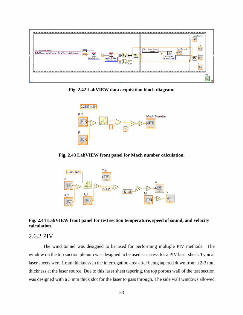
53

Fig. 2.42 LabVIEW data acquisition block diagram.

Fig. 2.43 LabVIEW front panel for Mach number calculation.

Fig. 2.44 LabVIEW front panel for test section temperature, speed of sound, and velocity

calculation.

2.6.2 PIV

The wind tunnel was designed to be used for performing multiple PIV methods. The

window on the top suction plenum was designed to be used as access for a PIV laser sheet. Typical

laser sheets were 1 mm thickness in the interrogation area after being tapered down from a 2-3 mm

thickness at the laser source. Due to this laser sheet tapering, the top porous wall of the test section

was designed with a 3 mm thick slot for the laser to pass through. The side wall windows allowed

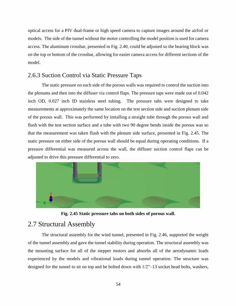
54

optical access for a PIV dual-frame or high speed camera to capture images around the airfoil or

models. The side of the tunnel without the motor controlling the model position is used for camera

access. The aluminum crossbar, presented in Fig. 2.40, could be adjusted so the bearing block was

on the top or bottom of the crossbar, allowing for easier camera access for different sections of the

model.

2.6.3 Suction Control via Static Pressure Taps

The static pressure on each side of the porous walls was required to control the suction into

the plenums and then into the diffuser via control flaps. The pressure taps were made out of 0.042

inch OD, 0.027 inch ID stainless steel tubing. The pressure tabs were designed to take

measurements at approximately the same location on the test section side and suction plenum side

of the porous wall. This was performed by installing a straight tube through the porous wall and

flush with the test section surface and a tube with two 90 degree bends inside the porous was so

that the measurement was taken flush with the plenum side surface, presented in Fig. 2.45. The

static pressure on either side of the porous wall should be equal during operating conditions. If a

pressure differential was measured across the wall, the diffuser suction control flaps can be

adjusted to drive this pressure differential to zero.

Fig. 2.45 Static pressure tabs on both sides of porous wall.

2.7 Structural Assembly

The structural assembly for the wind tunnel, presented in Fig. 2.46, supported the weight

of the tunnel assembly and gave the tunnel stability during operation. The structural assembly was

the mounting surface for all of the stepper motors and absorbs all of the aerodynamic loads

experienced by the models and vibrational loads during tunnel operation. The structure was

designed for the tunnel to sit on top and be bolted down with 1/2”–13 socket head bolts, washers,

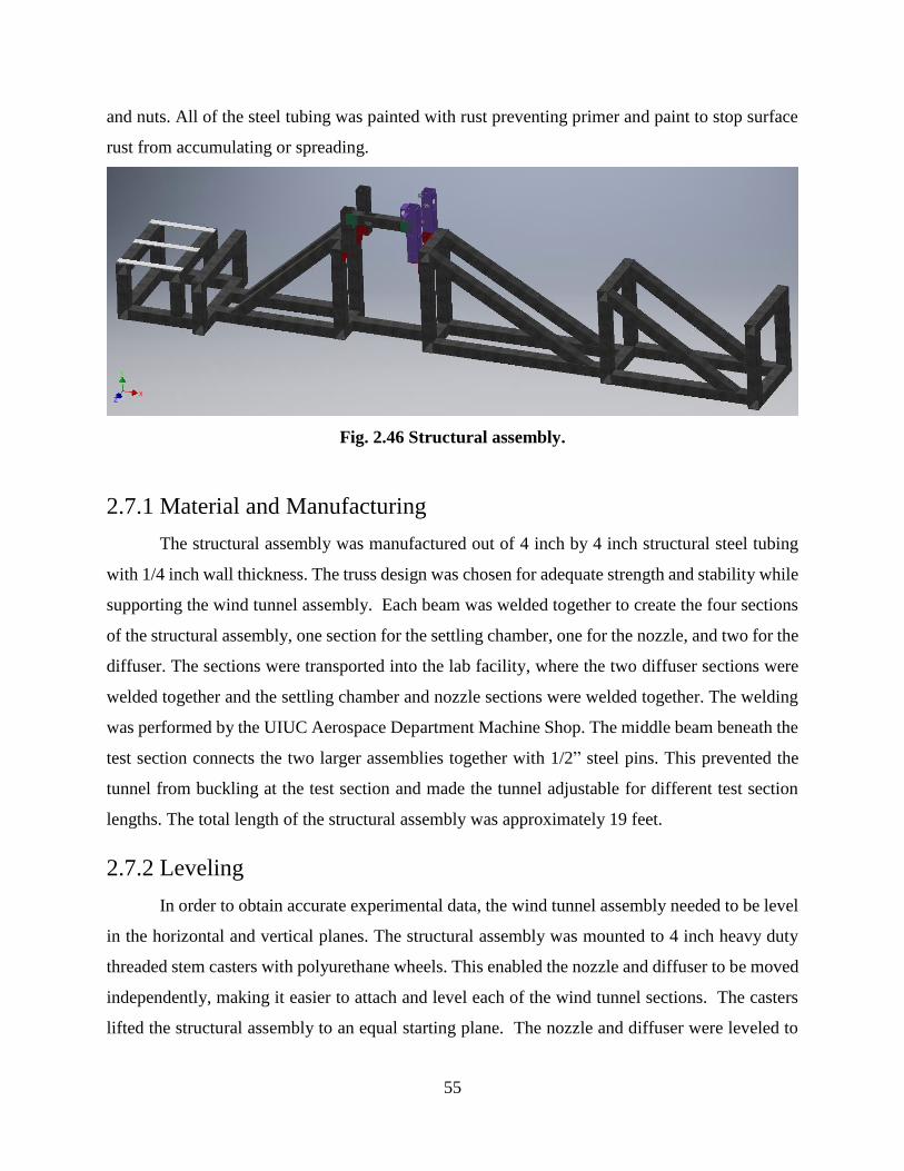
55

and nuts. All of the steel tubing was painted with rust preventing primer and paint to stop surface

rust from accumulating or spreading.

Fig. 2.46 Structural assembly.

2.7.1 Material and Manufacturing

The structural assembly was manufactured out of 4 inch by 4 inch structural steel tubing

with 1/4 inch wall thickness. The truss design was chosen for adequate strength and stability while

supporting the wind tunnel assembly. Each beam was welded together to create the four sections

of the structural assembly, one section for the settling chamber, one for the nozzle, and two for the

diffuser. The sections were transported into the lab facility, where the two diffuser sections were

welded together and the settling chamber and nozzle sections were welded together. The welding

was performed by the UIUC Aerospace Department Machine Shop. The middle beam beneath the

test section connects the two larger assemblies together with 1/2” steel pins. This prevented the

tunnel from buckling at the test section and made the tunnel adjustable for different test section

lengths. The total length of the structural assembly was approximately 19 feet.

2.7.2 Leveling

In order to obtain accurate experimental data, the wind tunnel assembly needed to be level

in the horizontal and vertical planes. The structural assembly was mounted to 4 inch heavy duty

threaded stem casters with polyurethane wheels. This enabled the nozzle and diffuser to be moved

independently, making it easier to attach and level each of the wind tunnel sections. The casters

lifted the structural assembly to an equal starting plane. The nozzle and diffuser were leveled to

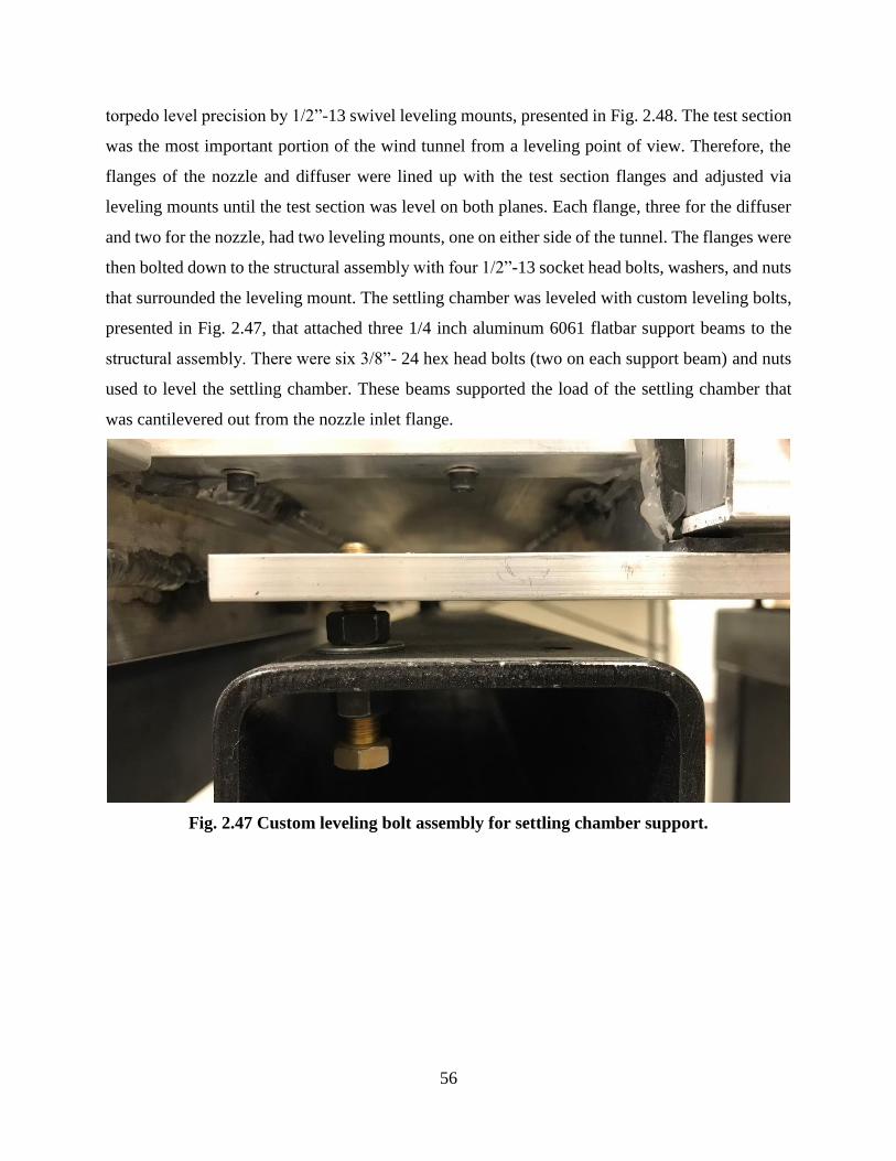
56

torpedo level precision by 1/2”-13 swivel leveling mounts, presented in Fig. 2.48. The test section

was the most important portion of the wind tunnel from a leveling point of view. Therefore, the

flanges of the nozzle and diffuser were lined up with the test section flanges and adjusted via

leveling mounts until the test section was level on both planes. Each flange, three for the diffuser

and two for the nozzle, had two leveling mounts, one on either side of the tunnel. The flanges were

then bolted down to the structural assembly with four 1/2”-13 socket head bolts, washers, and nuts

that surrounded the leveling mount. The settling chamber was leveled with custom leveling bolts,

presented in Fig. 2.47, that attached three 1/4 inch aluminum 6061 flatbar support beams to the

structural assembly. There were six 3/8”- 24 hex head bolts (two on each support beam) and nuts

used to level the settling chamber. These beams supported the load of the settling chamber that

was cantilevered out from the nozzle inlet flange.

Fig. 2.47 Custom leveling bolt assembly for settling chamber support.

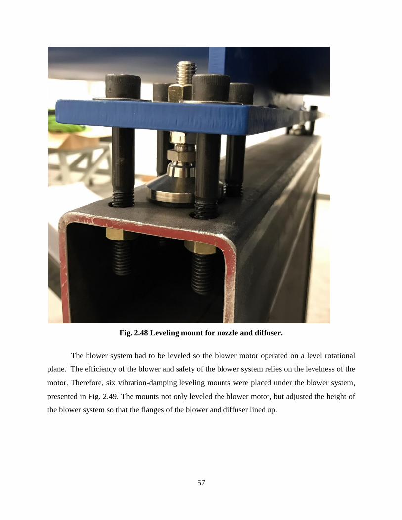
57

Fig. 2.48 Leveling mount for nozzle and diffuser.

The blower system had to be leveled so the blower motor operated on a level rotational

plane. The efficiency of the blower and safety of the blower system relies on the levelness of the

motor. Therefore, six vibration-damping leveling mounts were placed under the blower system,

presented in Fig. 2.49. The mounts not only leveled the blower motor, but adjusted the height of

the blower system so that the flanges of the blower and diffuser lined up.

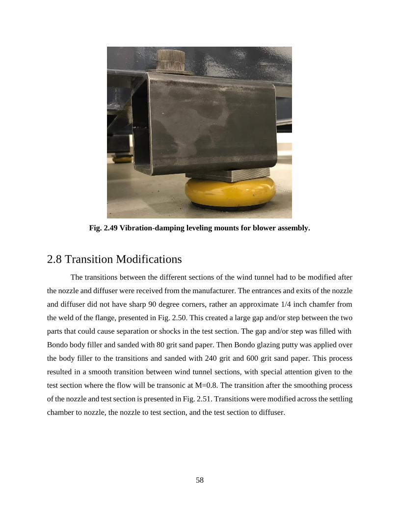
58

Fig. 2.49 Vibration-damping leveling mounts for blower assembly.

2.8 Transition Modifications

The transitions between the different sections of the wind tunnel had to be modified after

the nozzle and diffuser were received from the manufacturer. The entrances and exits of the nozzle

and diffuser did not have sharp 90 degree corners, rather an approximate 1/4 inch chamfer from

the weld of the flange, presented in Fig. 2.50. This created a large gap and/or step between the two

parts that could cause separation or shocks in the test section. The gap and/or step was filled with

Bondo body filler and sanded with 80 grit sand paper. Then Bondo glazing putty was applied over

the body filler to the transitions and sanded with 240 grit and 600 grit sand paper. This process

resulted in a smooth transition between wind tunnel sections, with special attention given to the

test section where the flow will be transonic at M=0.8. The transition after the smoothing process

of the nozzle and test section is presented in Fig. 2.51. Transitions were modified across the settling

chamber to nozzle, the nozzle to test section, and the test section to diffuser.

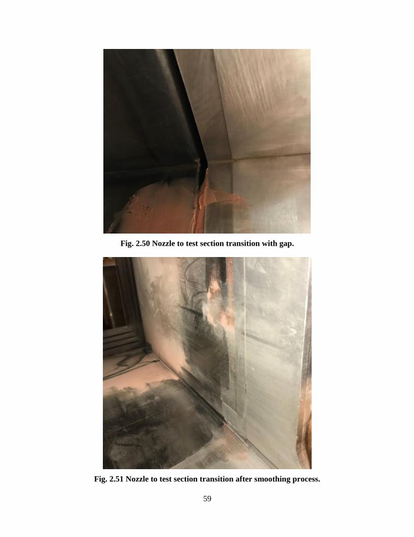
59

Fig. 2.50 Nozzle to test section transition with gap.

Fig. 2.51 Nozzle to test section transition after smoothing process.

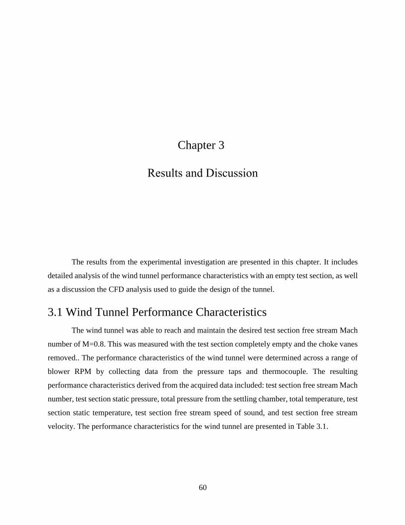
60

Chapter 3

Results and Discussion

The results from the experimental investigation are presented in this chapter. It includes

detailed analysis of the wind tunnel performance characteristics with an empty test section, as well

as a discussion the CFD analysis used to guide the design of the tunnel.

3.1 Wind Tunnel Performance Characteristics

The wind tunnel was able to reach and maintain the desired test section free stream Mach

number of M=0.8. This was measured with the test section completely empty and the choke vanes

removed.. The performance characteristics of the wind tunnel were determined across a range of

blower RPM by collecting data from the pressure taps and thermocouple. The resulting

performance characteristics derived from the acquired data included: test section free stream Mach

number, test section static pressure, total pressure from the settling chamber, total temperature, test

section static temperature, test section free stream speed of sound, and test section free stream

velocity. The performance characteristics for the wind tunnel are presented in Table 3.1.

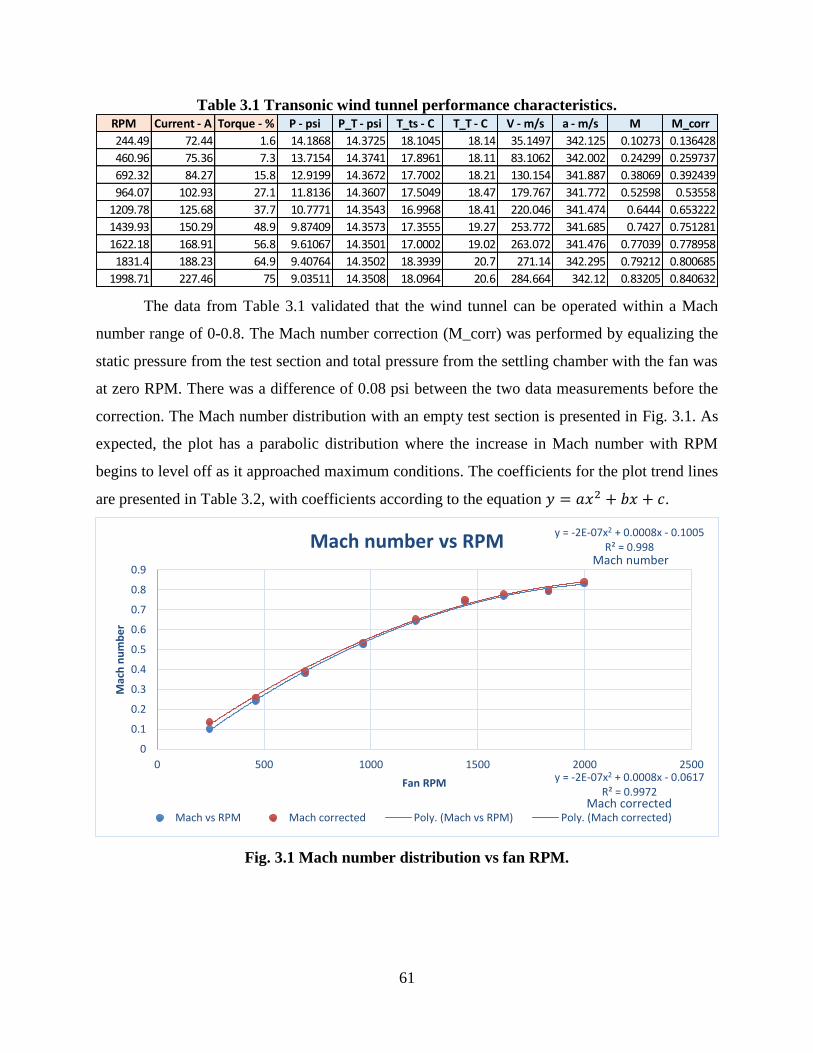
61

Table 3.1 Transonic wind tunnel performance characteristics.

The data from Table 3.1 validated that the wind tunnel can be operated within a Mach

number range of 0-0.8. The Mach number correction (M_corr) was performed by equalizing the

static pressure from the test section and total pressure from the settling chamber with the fan was

at zero RPM. There was a difference of 0.08 psi between the two data measurements before the

correction. The Mach number distribution with an empty test section is presented in Fig. 3.1. As

expected, the plot has a parabolic distribution where the increase in Mach number with RPM

begins to level off as it approached maximum conditions. The coefficients for the plot trend lines

are presented in Table 3.2, with coefficients according to the equation 𝑦 = 𝑎𝑥2 + 𝑏𝑥 + 𝑐.

Fig. 3.1 Mach number distribution vs fan RPM.

RPM Current - A Torque - % P - psi P_T - psi T_ts - C T_T - C V - m/s a - m/s M M_corr

244.49 72.44 1.6 14.1868 14.3725 18.1045 18.14 35.1497 342.125 0.10273 0.136428

460.96 75.36 7.3 13.7154 14.3741 17.8961 18.11 83.1062 342.002 0.24299 0.259737

692.32 84.27 15.8 12.9199 14.3672 17.7002 18.21 130.154 341.887 0.38069 0.392439

964.07 102.93 27.1 11.8136 14.3607 17.5049 18.47 179.767 341.772 0.52598 0.53558

1209.78 125.68 37.7 10.7771 14.3543 16.9968 18.41 220.046 341.474 0.6444 0.653222

1439.93 150.29 48.9 9.87409 14.3573 17.3555 19.27 253.772 341.685 0.7427 0.751281

1622.18 168.91 56.8 9.61067 14.3501 17.0002 19.02 263.072 341.476 0.77039 0.778958

1831.4 188.23 64.9 9.40764 14.3502 18.3939 20.7 271.14 342.295 0.79212 0.800685

1998.71 227.46 75 9.03511 14.3508 18.0964 20.6 284.664 342.12 0.83205 0.840632

y = -2E-07x2 + 0.0008x - 0.1005R² = 0.998

y = -2E-07x2 + 0.0008x - 0.0617R² = 0.9972

0

0.1

0.2

0.3

0.4

0.5

0.6

0.7

0.8

0.9

0 500 1000 1500 2000 2500

Mac

h n

um

be

r

Fan RPM

Mach number vs RPM

Mach vs RPM Mach corrected Poly. (Mach vs RPM) Poly. (Mach corrected)Mach corrected

Mach number

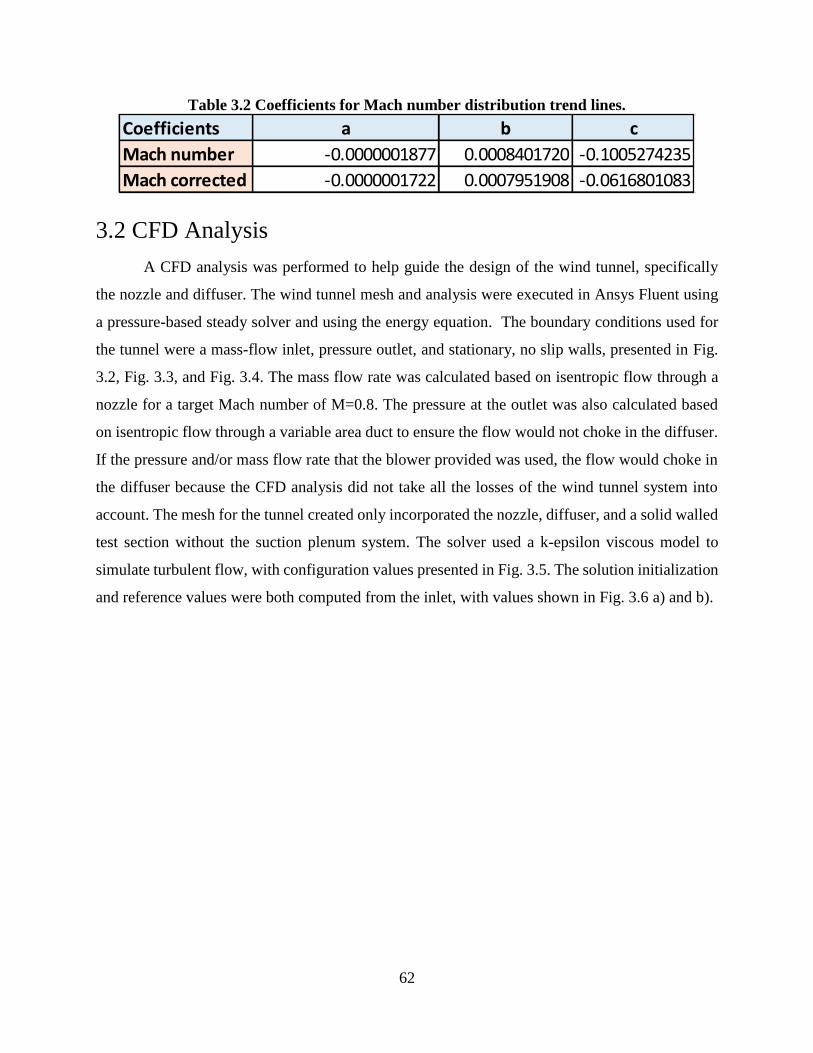
62

Table 3.2 Coefficients for Mach number distribution trend lines.

3.2 CFD Analysis

A CFD analysis was performed to help guide the design of the wind tunnel, specifically

the nozzle and diffuser. The wind tunnel mesh and analysis were executed in Ansys Fluent using

a pressure-based steady solver and using the energy equation. The boundary conditions used for

the tunnel were a mass-flow inlet, pressure outlet, and stationary, no slip walls, presented in Fig.

3.2, Fig. 3.3, and Fig. 3.4. The mass flow rate was calculated based on isentropic flow through a

nozzle for a target Mach number of M=0.8. The pressure at the outlet was also calculated based

on isentropic flow through a variable area duct to ensure the flow would not choke in the diffuser.

If the pressure and/or mass flow rate that the blower provided was used, the flow would choke in

the diffuser because the CFD analysis did not take all the losses of the wind tunnel system into

account. The mesh for the tunnel created only incorporated the nozzle, diffuser, and a solid walled

test section without the suction plenum system. The solver used a k-epsilon viscous model to

simulate turbulent flow, with configuration values presented in Fig. 3.5. The solution initialization

and reference values were both computed from the inlet, with values shown in Fig. 3.6 a) and b).

Coefficients a b c

Mach number -0.0000001877 0.0008401720 -0.1005274235

Mach corrected -0.0000001722 0.0007951908 -0.0616801083

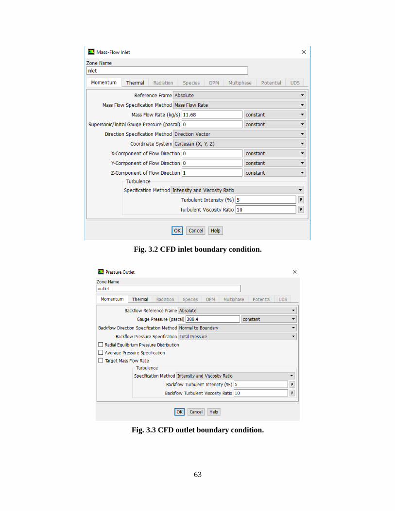
63

Fig. 3.2 CFD inlet boundary condition.

Fig. 3.3 CFD outlet boundary condition.

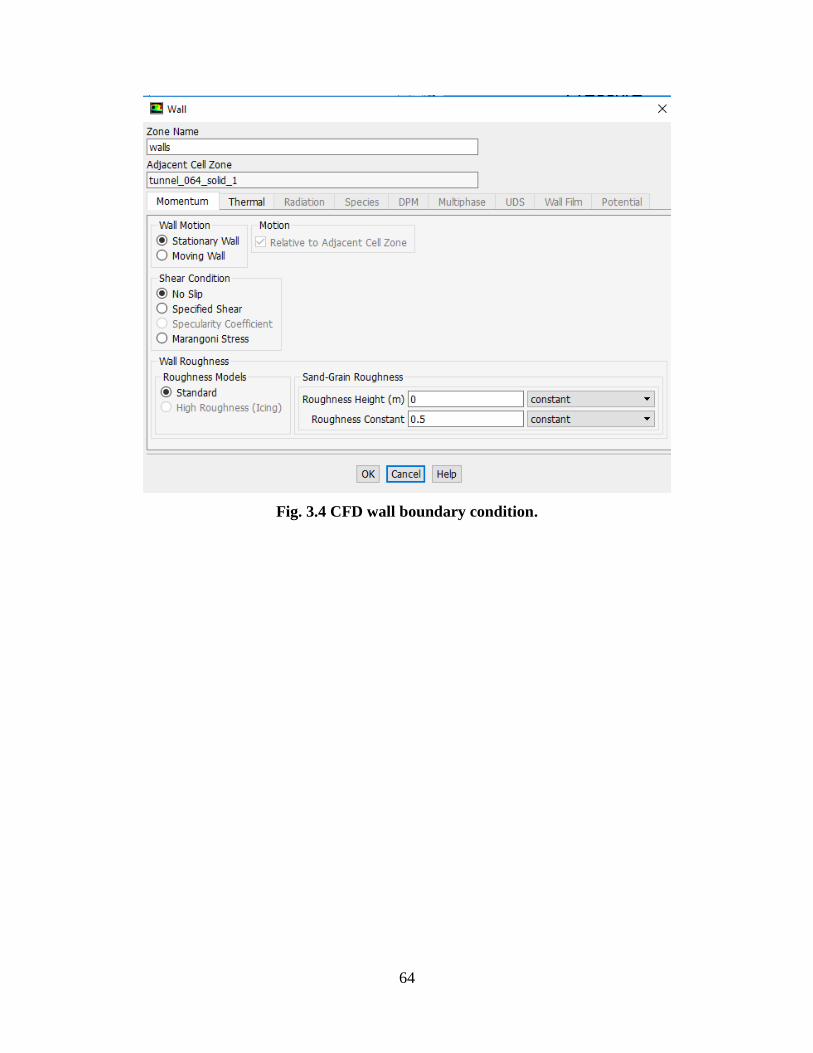
64

Fig. 3.4 CFD wall boundary condition.

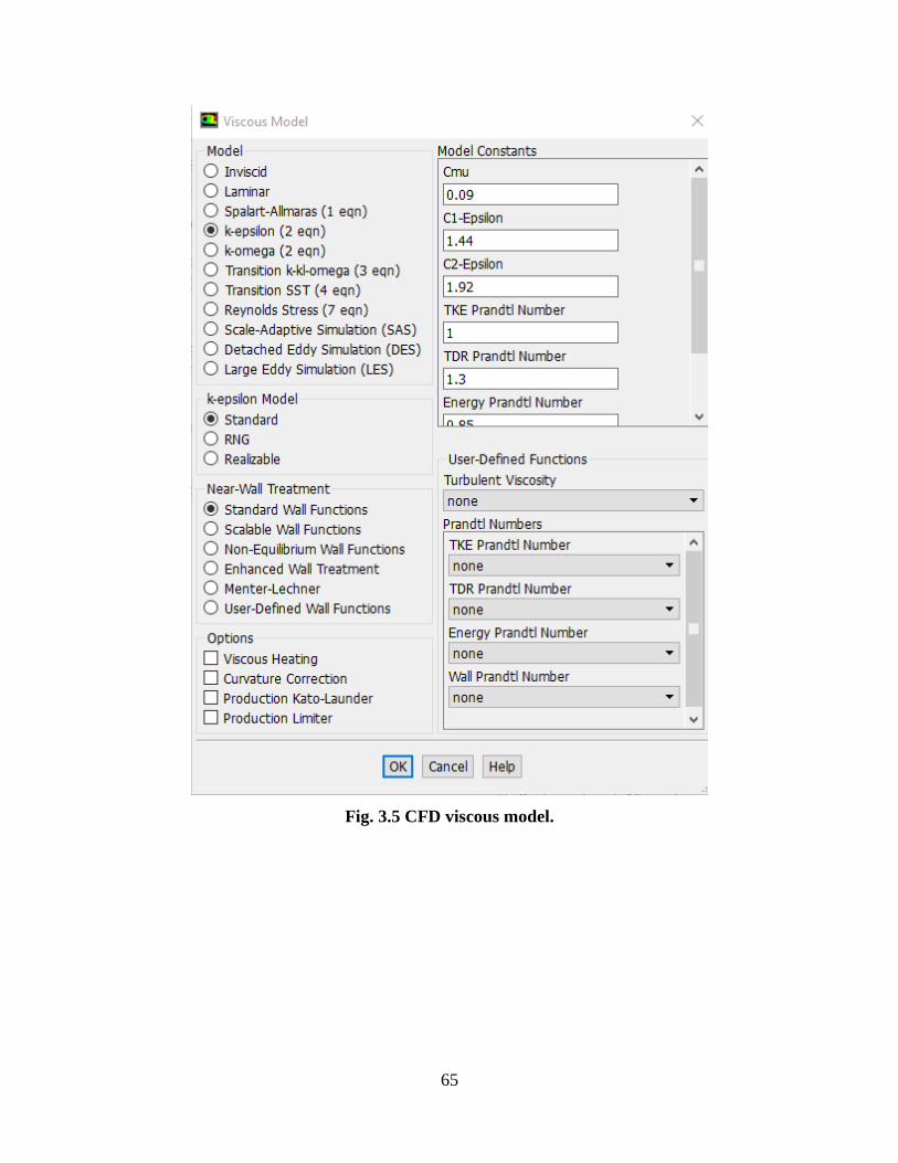
65

Fig. 3.5 CFD viscous model.

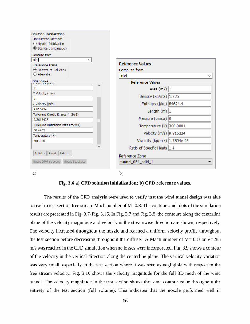
66

Fig. 3.6 a) CFD solution initialization; b) CFD reference values.

The results of the CFD analysis were used to verify that the wind tunnel design was able

to reach a test section free stream Mach number of M=0.8. The contours and plots of the simulation

results are presented in Fig. 3.7-Fig. 3.15. In Fig. 3.7 and Fig. 3.8, the contours along the centerline

plane of the velocity magnitude and velocity in the streamwise direction are shown, respectively.

The velocity increased throughout the nozzle and reached a uniform velocity profile throughout

the test section before decreasing throughout the diffuser. A Mach number of M=0.83 or V=285

m/s was reached in the CFD simulation when no losses were incorporated. Fig. 3.9 shows a contour

of the velocity in the vertical direction along the centerline plane. The vertical velocity variation

was very small, especially in the test section where it was seen as negligible with respect to the

free stream velocity. Fig. 3.10 shows the velocity magnitude for the full 3D mesh of the wind

tunnel. The velocity magnitude in the test section shows the same contour value throughout the

entirety of the test section (full volume). This indicates that the nozzle performed well in

a) b)

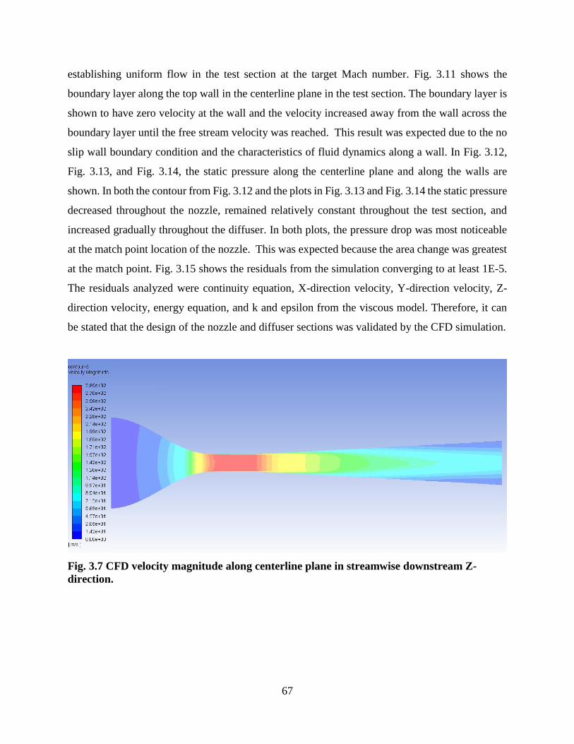
67

establishing uniform flow in the test section at the target Mach number. Fig. 3.11 shows the

boundary layer along the top wall in the centerline plane in the test section. The boundary layer is

shown to have zero velocity at the wall and the velocity increased away from the wall across the

boundary layer until the free stream velocity was reached. This result was expected due to the no

slip wall boundary condition and the characteristics of fluid dynamics along a wall. In Fig. 3.12,

Fig. 3.13, and Fig. 3.14, the static pressure along the centerline plane and along the walls are

shown. In both the contour from Fig. 3.12 and the plots in Fig. 3.13 and Fig. 3.14 the static pressure

decreased throughout the nozzle, remained relatively constant throughout the test section, and

increased gradually throughout the diffuser. In both plots, the pressure drop was most noticeable

at the match point location of the nozzle. This was expected because the area change was greatest

at the match point. Fig. 3.15 shows the residuals from the simulation converging to at least 1E-5.

The residuals analyzed were continuity equation, X-direction velocity, Y-direction velocity, Z-

direction velocity, energy equation, and k and epsilon from the viscous model. Therefore, it can

be stated that the design of the nozzle and diffuser sections was validated by the CFD simulation.

Fig. 3.7 CFD velocity magnitude along centerline plane in streamwise downstream Z-

direction.

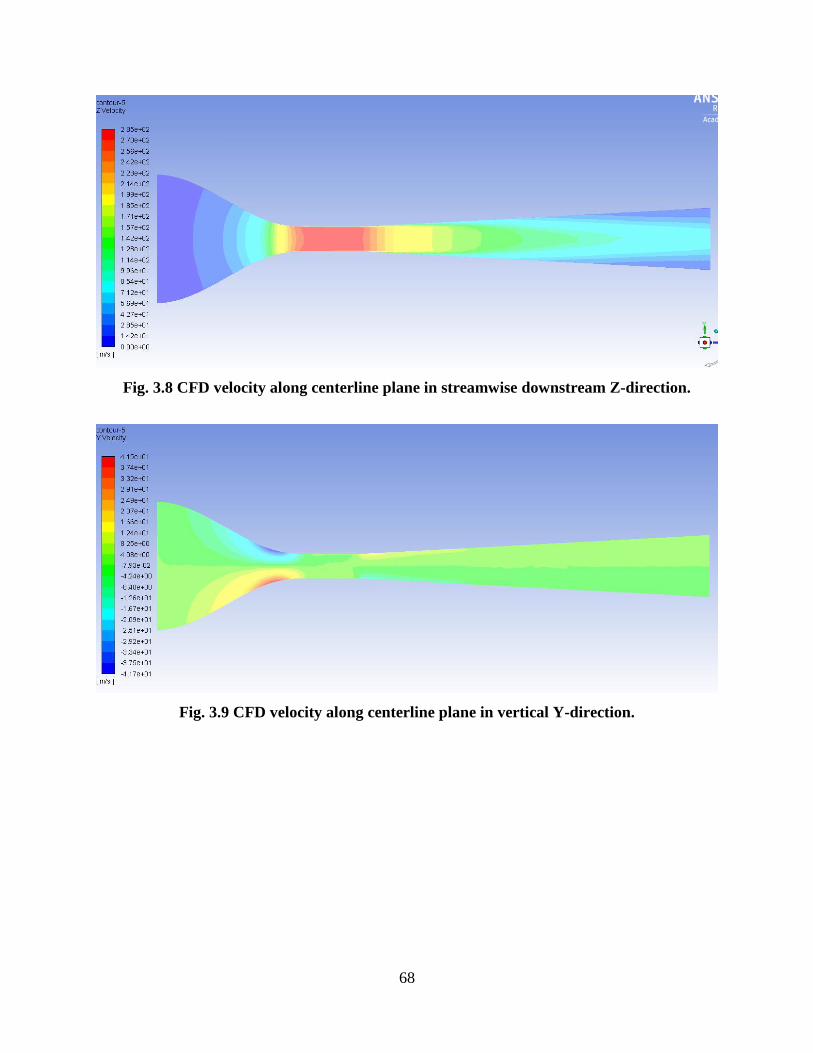
68

Fig. 3.8 CFD velocity along centerline plane in streamwise downstream Z-direction.

Fig. 3.9 CFD velocity along centerline plane in vertical Y-direction.

69

Fig. 3.10 CFD velocity magnitude for full 3D tunnel mesh.

Fig. 3.11 CFD velocity magnitude on centerline plane in streamwise downstream Z-

direction, displaying the boundary layer.

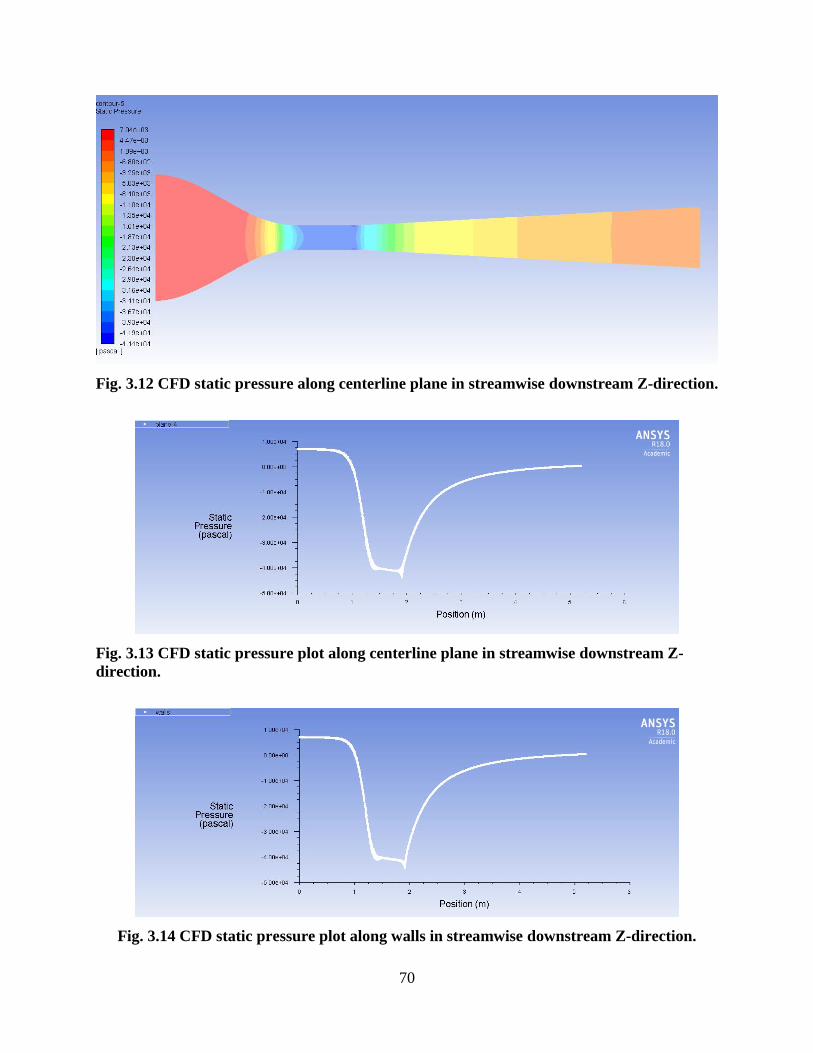
70

Fig. 3.12 CFD static pressure along centerline plane in streamwise downstream Z-direction.

Fig. 3.13 CFD static pressure plot along centerline plane in streamwise downstream Z-

direction.

Fig. 3.14 CFD static pressure plot along walls in streamwise downstream Z-direction.

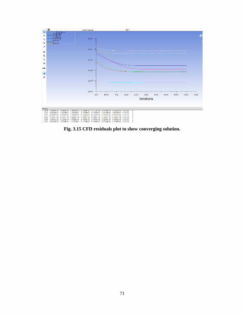
71

Fig. 3.15 CFD residuals plot to show converging solution.

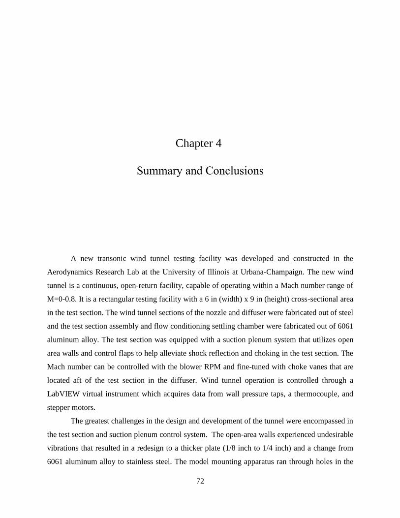
72

Chapter 4

Summary and Conclusions

A new transonic wind tunnel testing facility was developed and constructed in the

Aerodynamics Research Lab at the University of Illinois at Urbana-Champaign. The new wind

tunnel is a continuous, open-return facility, capable of operating within a Mach number range of

M=0-0.8. It is a rectangular testing facility with a 6 in (width) x 9 in (height) cross-sectional area

in the test section. The wind tunnel sections of the nozzle and diffuser were fabricated out of steel

and the test section assembly and flow conditioning settling chamber were fabricated out of 6061

aluminum alloy. The test section was equipped with a suction plenum system that utilizes open

area walls and control flaps to help alleviate shock reflection and choking in the test section. The

Mach number can be controlled with the blower RPM and fine-tuned with choke vanes that are

located aft of the test section in the diffuser. Wind tunnel operation is controlled through a

LabVIEW virtual instrument which acquires data from wall pressure taps, a thermocouple, and

stepper motors.

The greatest challenges in the design and development of the tunnel were encompassed in

the test section and suction plenum control system. The open-area walls experienced undesirable

vibrations that resulted in a redesign to a thicker plate (1/8 inch to 1/4 inch) and a change from

6061 aluminum alloy to stainless steel. The model mounting apparatus ran through holes in the

73

glass windows and was supported by structural cross beams. A CAD FEA was performed on the

mounting spar to ensure the load was transferred to the structure and the deflection did not contact

the glass. Another significant challenge was the design of the high contraction ratio nozzle. CFD

and previous experimental data were used to design the nozzle to produce uniform flow through

the test section with minimal losses.

A 250 hp centrifugal blower system was selected to drive the tunnel because of its flexible

performance envelope and pressure recover capabilities. A conservative estimate was used for the

blower power and CFM to compensate for all the losses that occur throughout the tunnel while

still sustaining the target Mach number. The flow conditioning for the wind tunnel was achieved

in the settling chamber through the use of a flow straightening honeycomb and three turbulence

reducing screens. The screens were aft of the honeycomb, decreasing in wire diameter and

increasing in mesh density with each successive screen downstream. The diffuser transitioned from

the rectangular test section to the circular entrance into the blower. Diffuser expansion angles of

3.75 degrees (horizontal transition) and 3.09 degrees (vertical transition) were chosen for the

benefits of both flow steadiness and pressure recovery.

The validity of the new transonic wind tunnel facility as a functional test bed was

demonstrated through a series of benchmarking tests with an empty test section. The performance

characteristics were collected for different blower fan RPM up to the nominal condition of Mach

0.8. The wind tunnel was found to produce a constant Mach number in the test section when set to

a specific RPM. In order to validate the production of uniform flow in the test section, further

testing, such as PIV, will need to be performed.

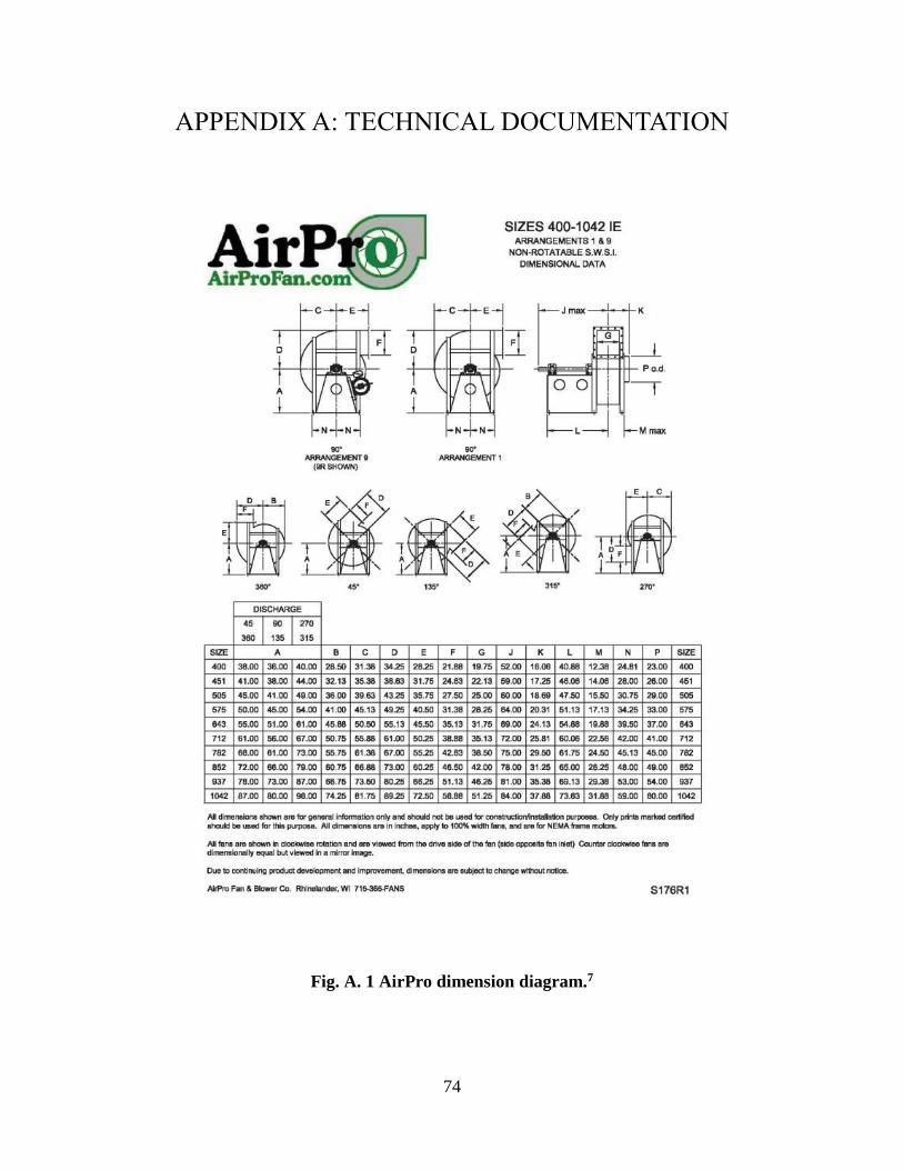
74

APPENDIX A: TECHNICAL DOCUMENTATION

Fig. A. 1 AirPro dimension diagram.7

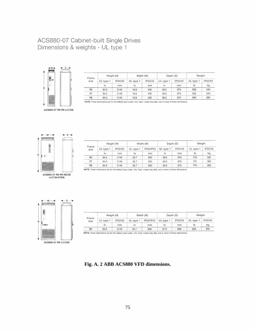
75

Fig. A. 2 ABB ACS880 VFD dimensions.

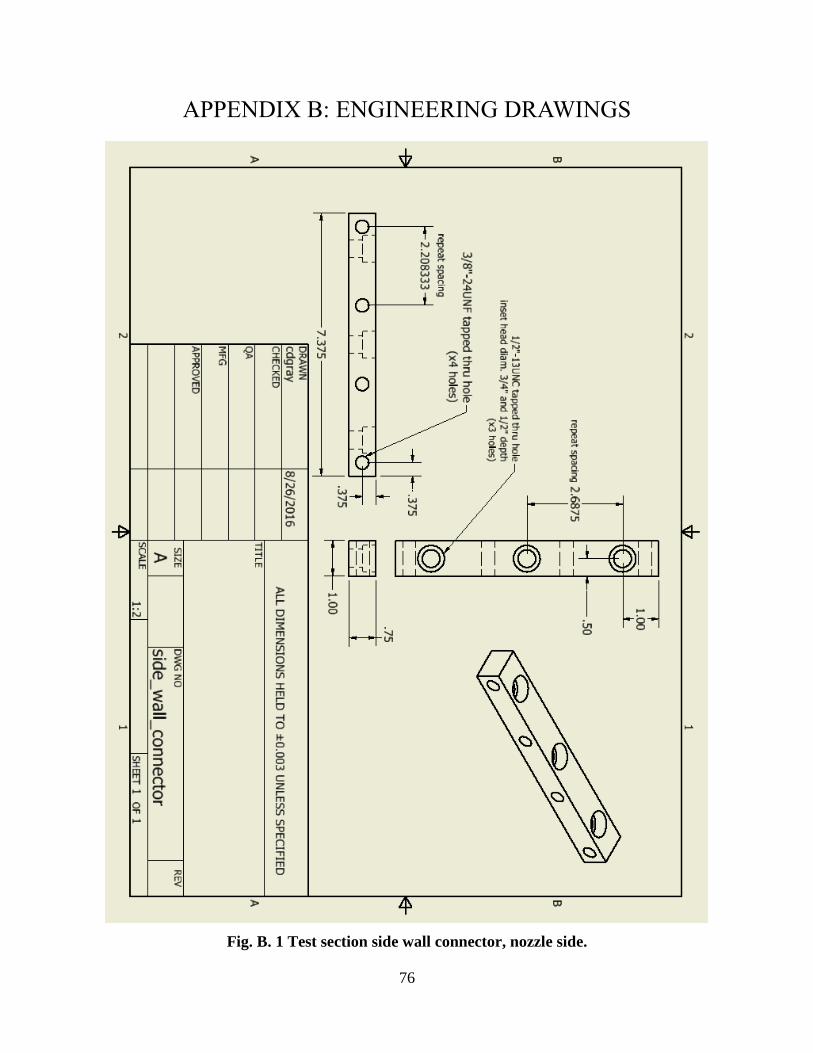
76

APPENDIX B: ENGINEERING DRAWINGS

Fig. B. 1 Test section side wall connector, nozzle side.

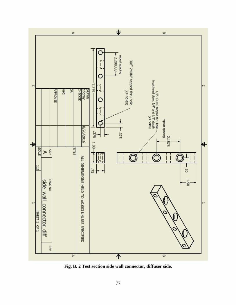
77

Fig. B. 2 Test section side wall connector, diffuser side.

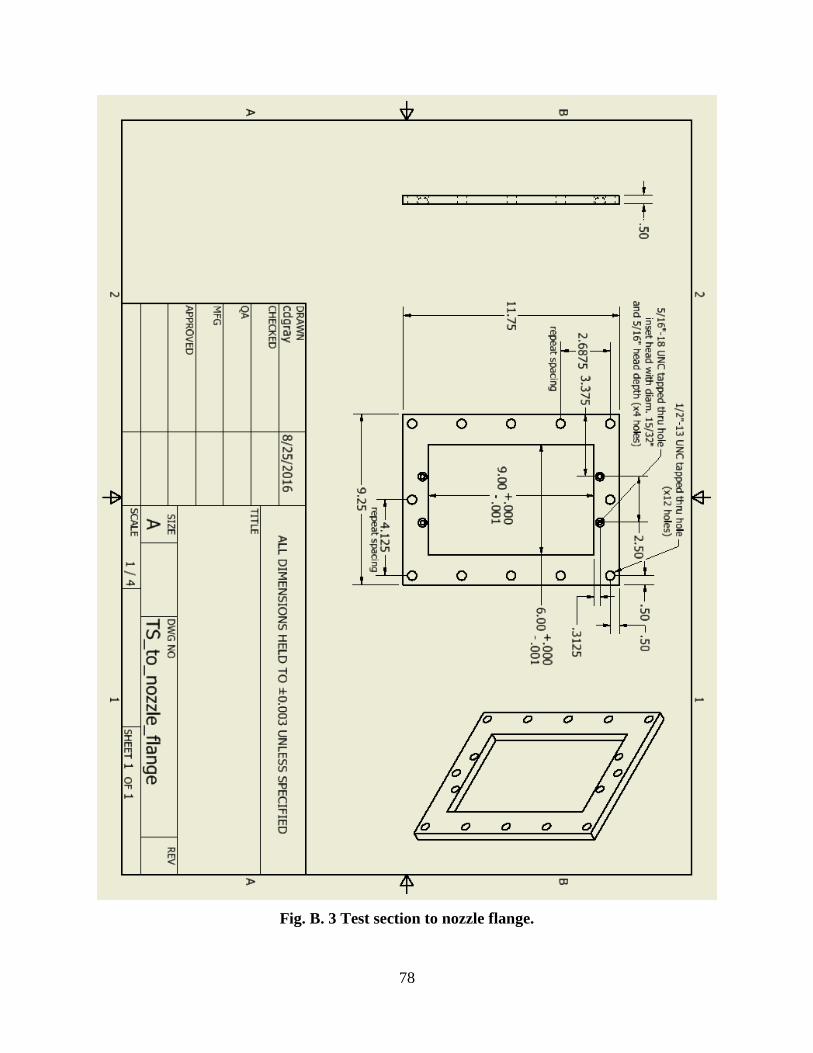
78

Fig. B. 3 Test section to nozzle flange.

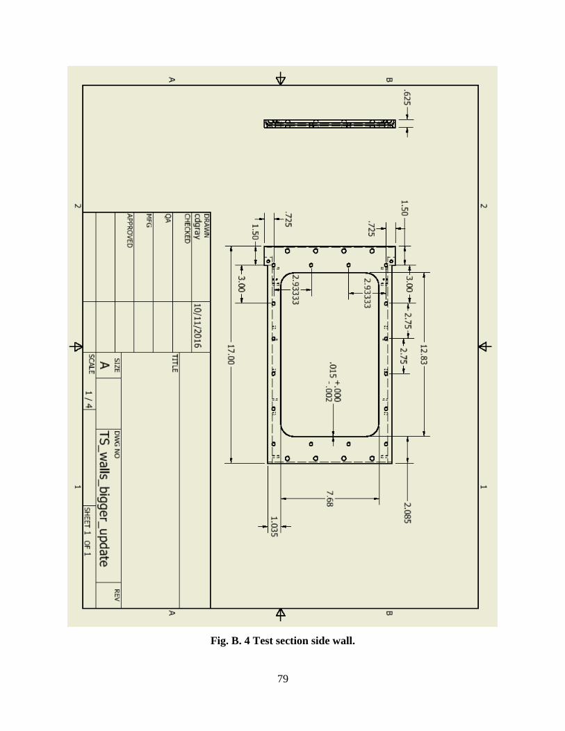
79

Fig. B. 4 Test section side wall.

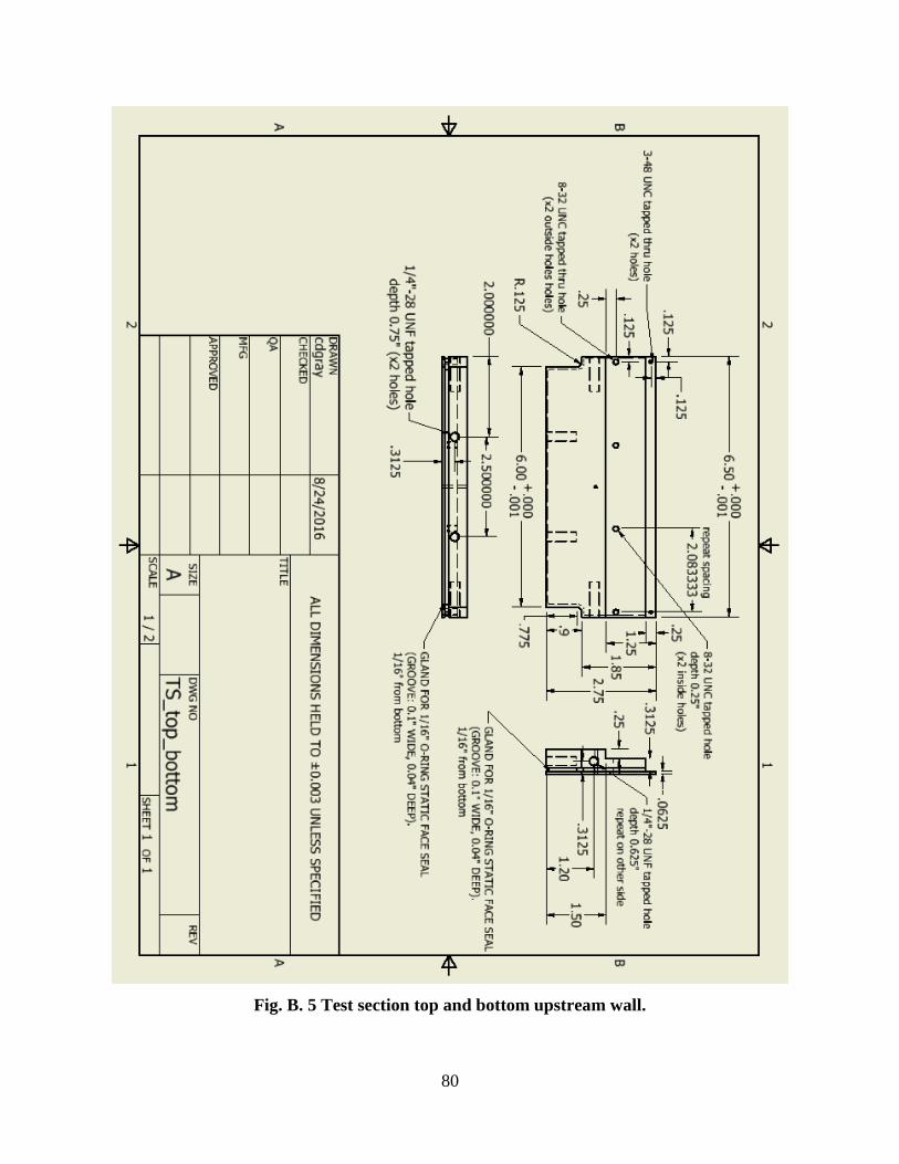
80

Fig. B. 5 Test section top and bottom upstream wall.

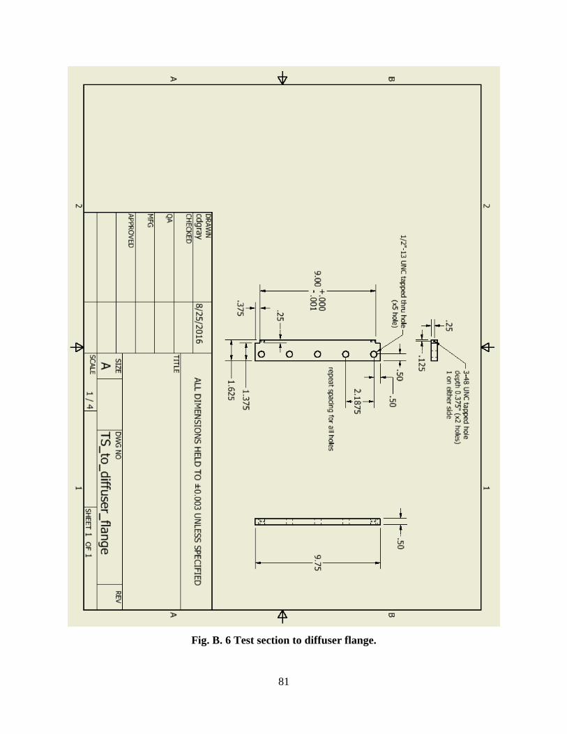
81

Fig. B. 6 Test section to diffuser flange.

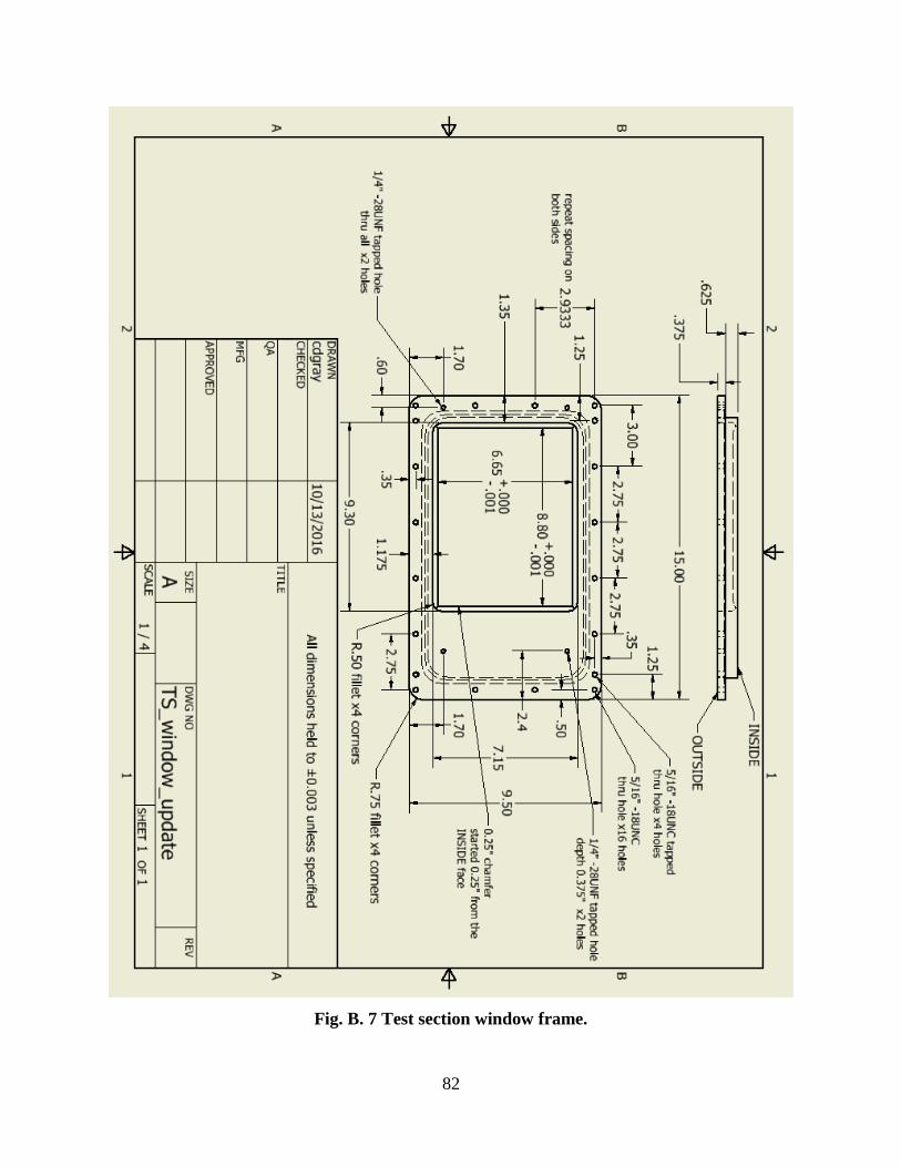
82

Fig. B. 7 Test section window frame.

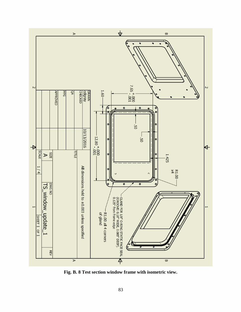
83

Fig. B. 8 Test section window frame with isometric view.

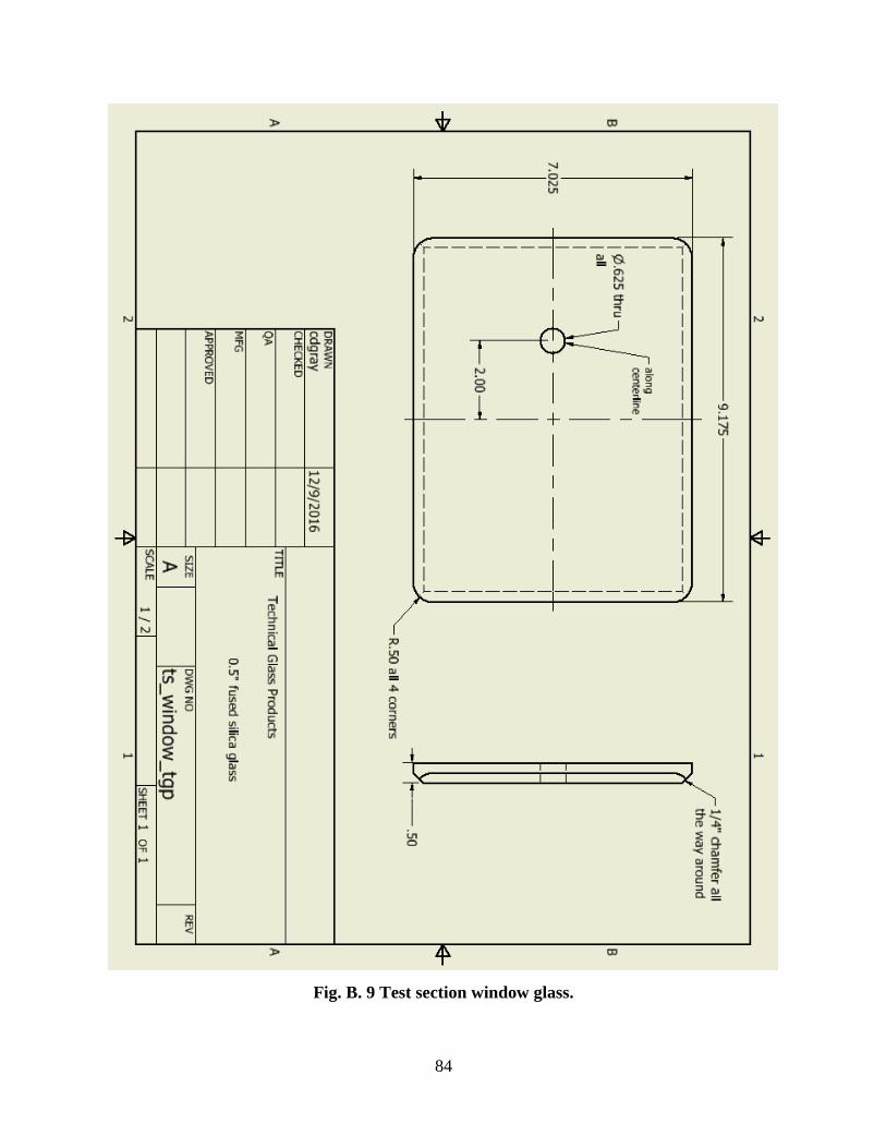
84

Fig. B. 9 Test section window glass.

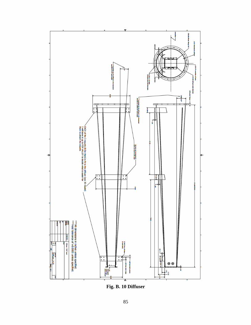
85

Fig. B. 10 Diffuser

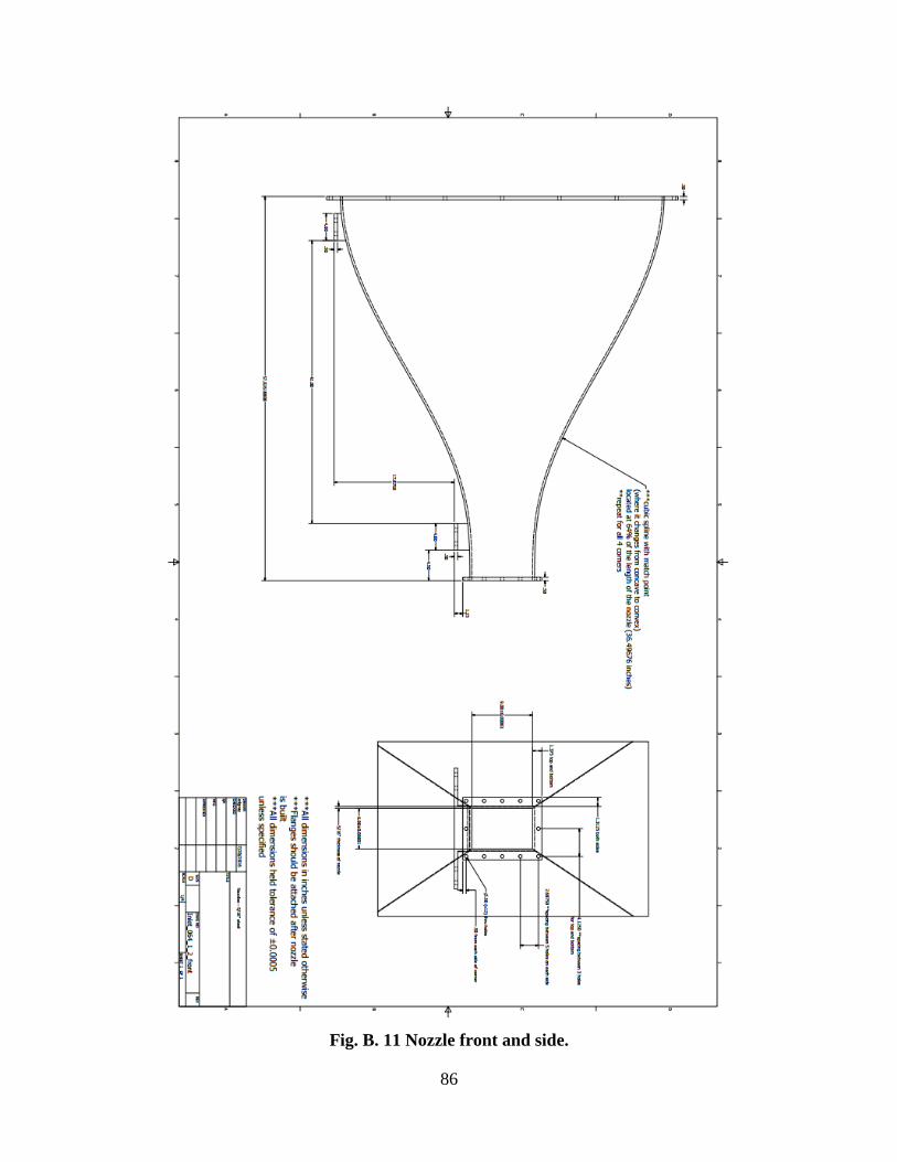
86

Fig. B. 11 Nozzle front and side.

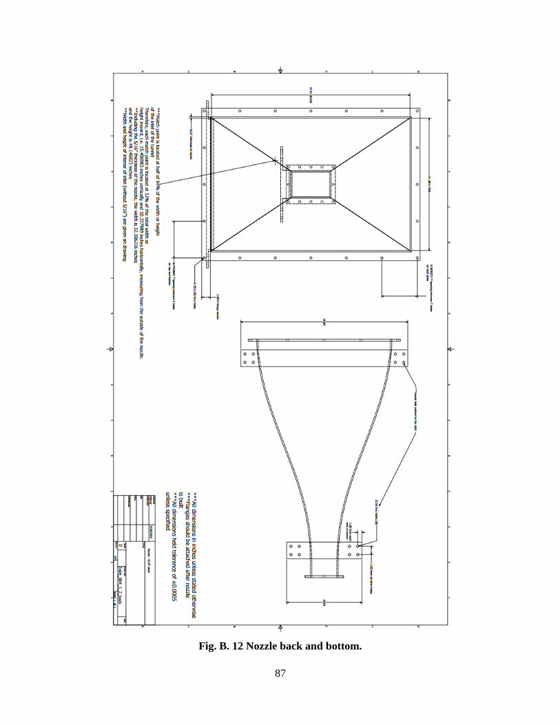
87

Fig. B. 12 Nozzle back and bottom.

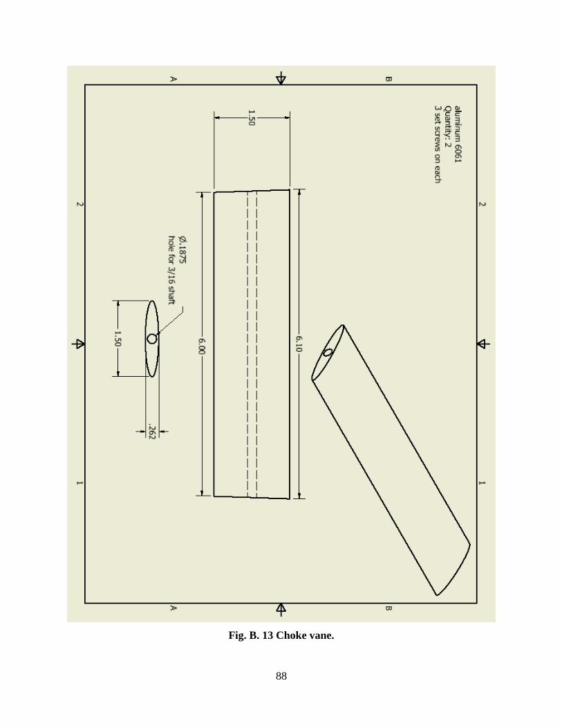
88

Fig. B. 13 Choke vane.

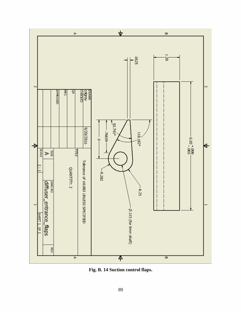
89

Fig. B. 14 Suction control flaps.

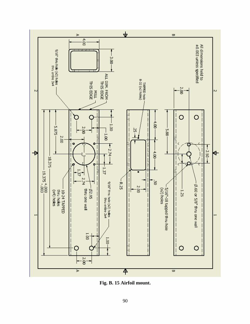
90

Fig. B. 15 Airfoil mount.

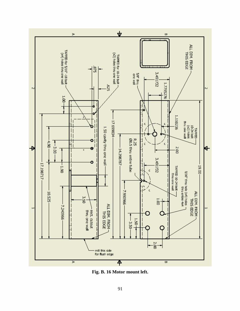
91

Fig. B. 16 Motor mount left.

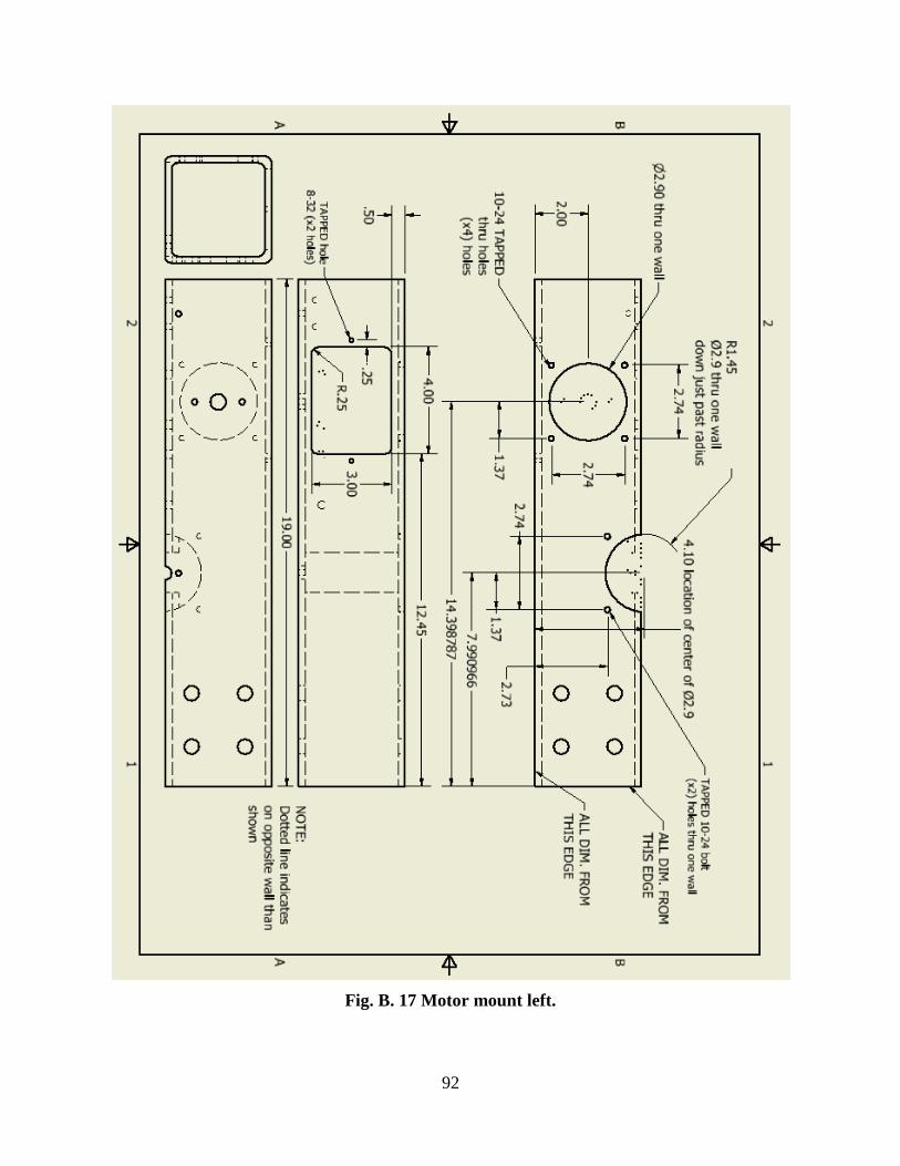
92

Fig. B. 17 Motor mount left.

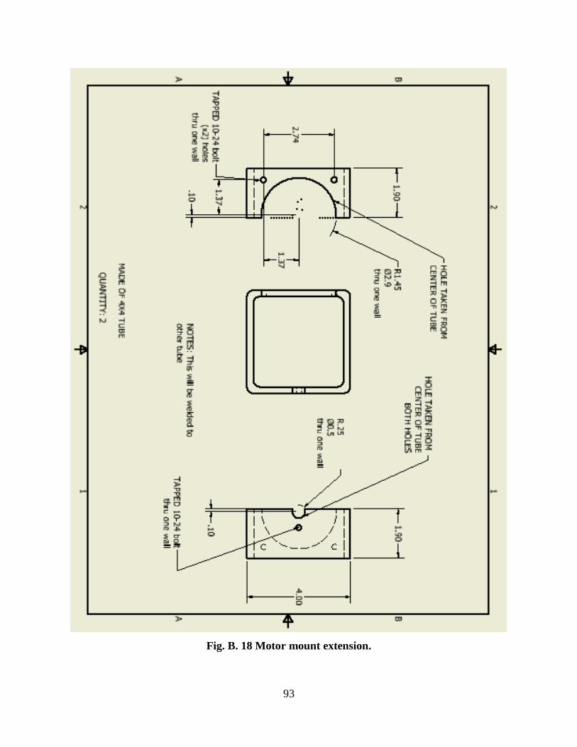
93

Fig. B. 18 Motor mount extension.

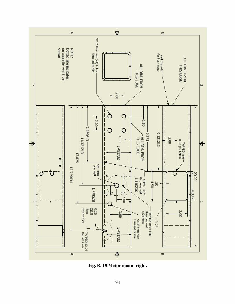
94

Fig. B. 19 Motor mount right.

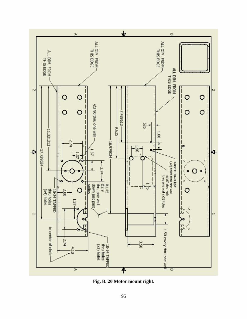
95

Fig. B. 20 Motor mount right.

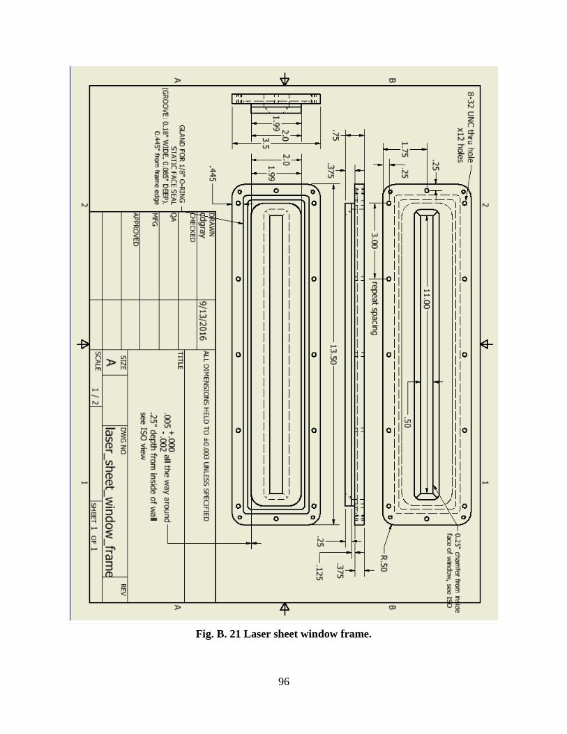
96

Fig. B. 21 Laser sheet window frame.

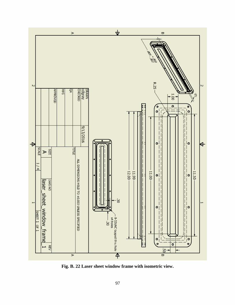
97

Fig. B. 22 Laser sheet window frame with isometric view.

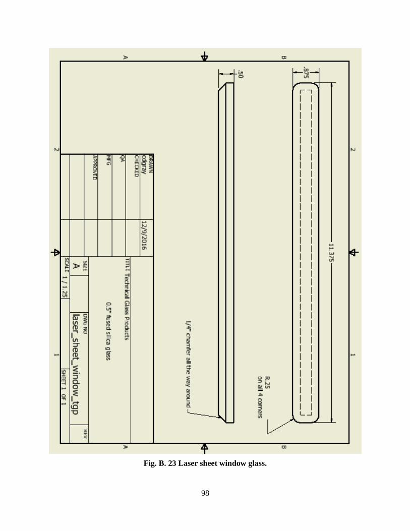
98

Fig. B. 23 Laser sheet window glass.

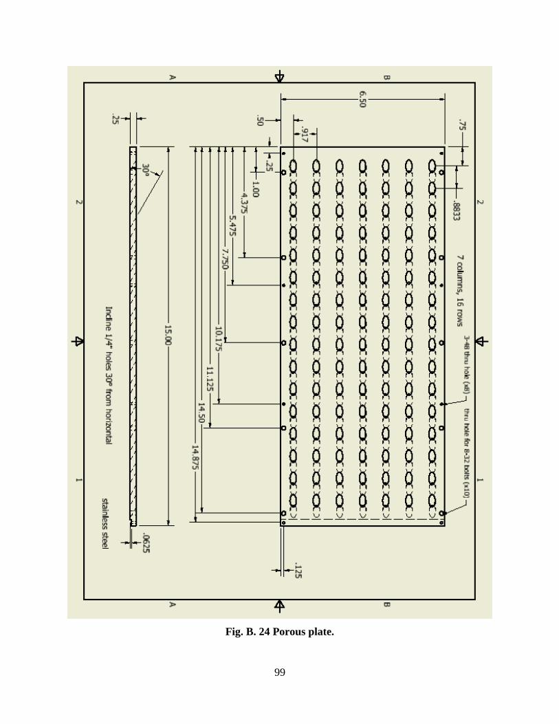
99

Fig. B. 24 Porous plate.

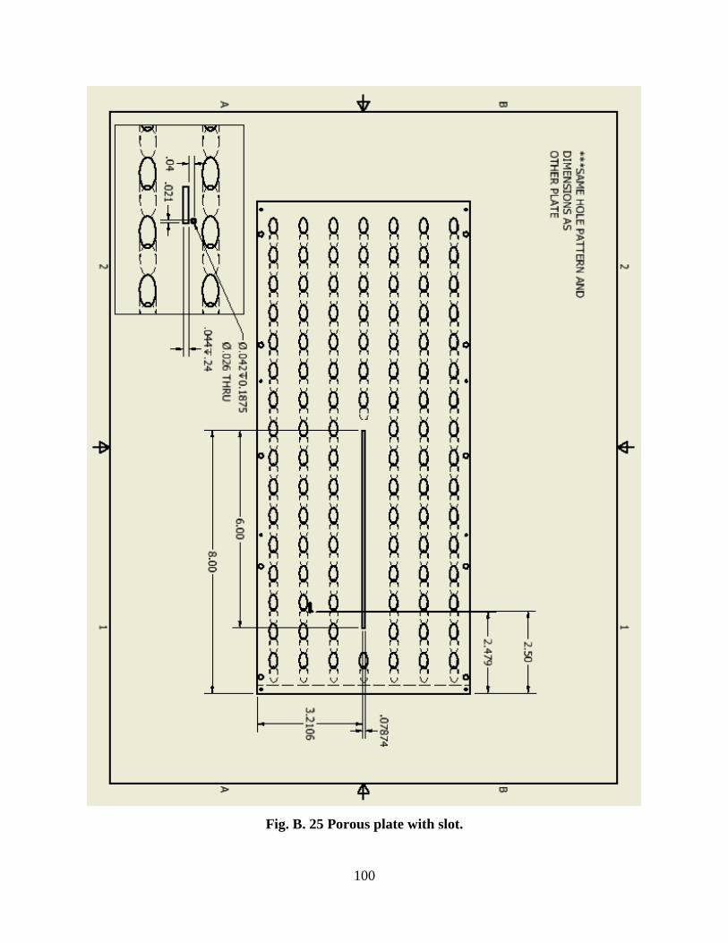
100

Fig. B. 25 Porous plate with slot.

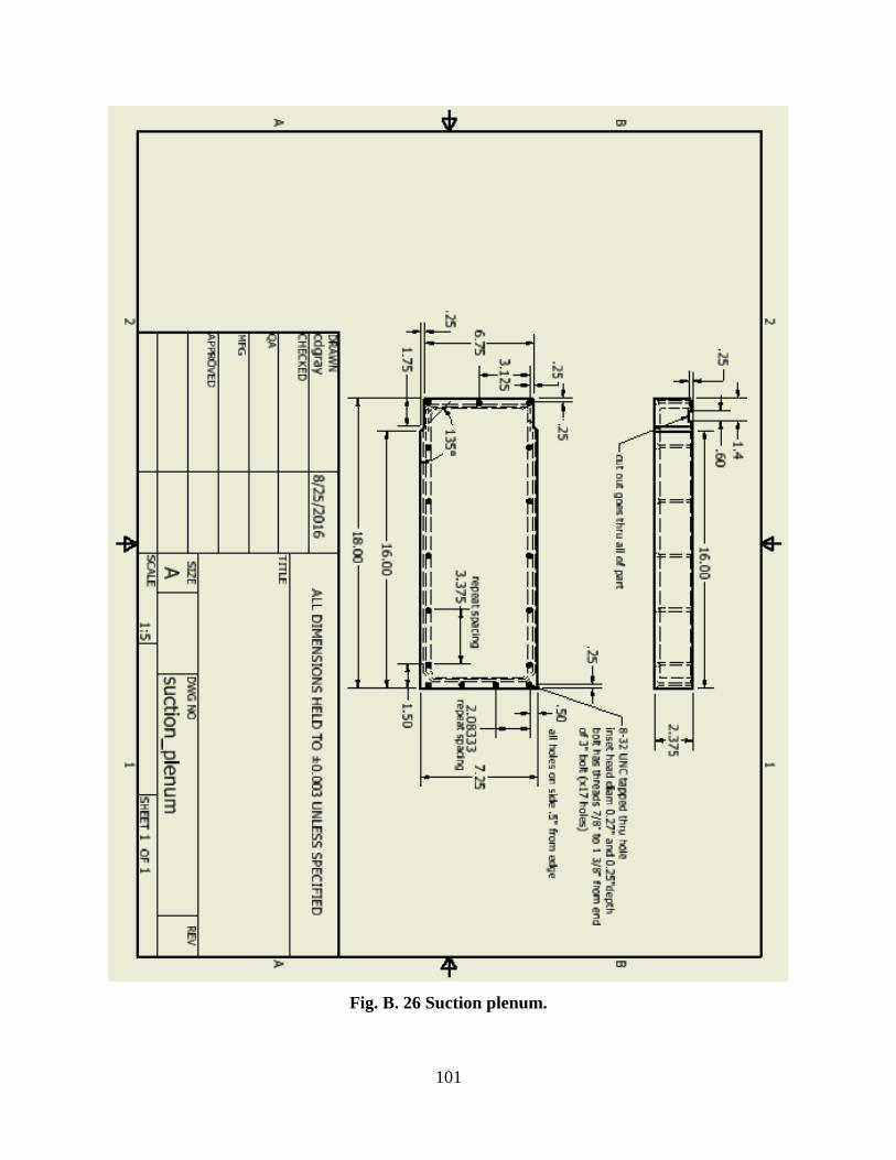
101

Fig. B. 26 Suction plenum.

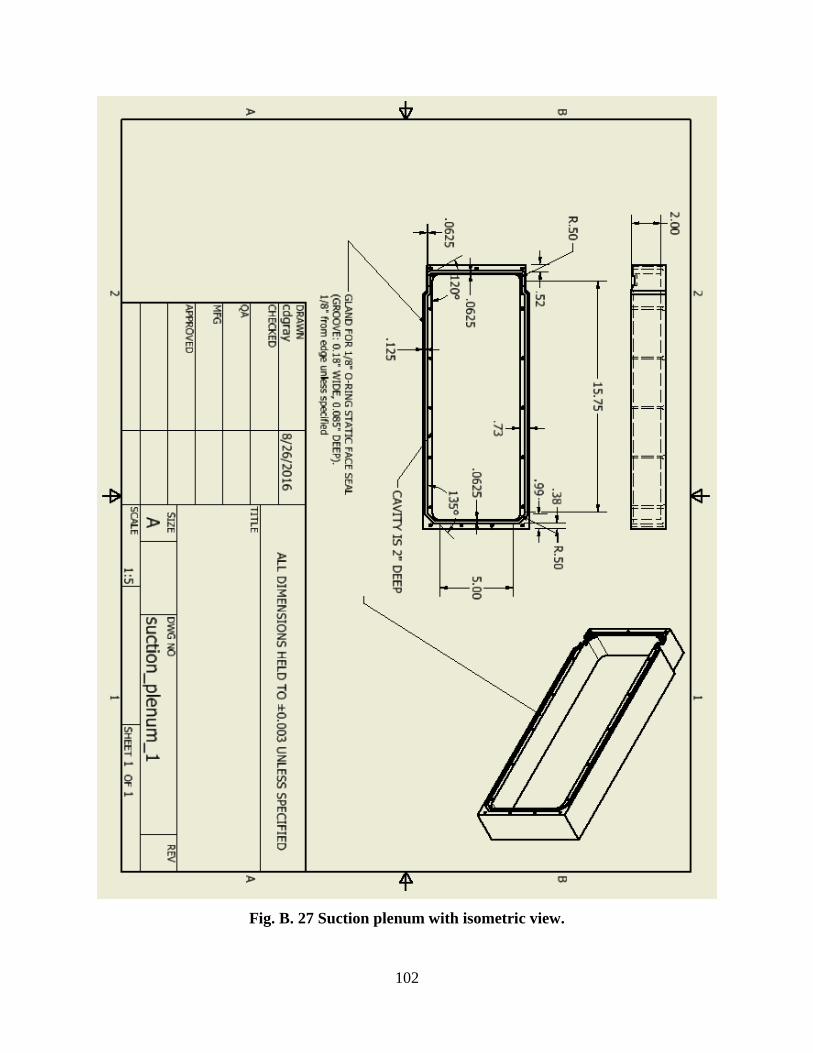
102

Fig. B. 27 Suction plenum with isometric view.

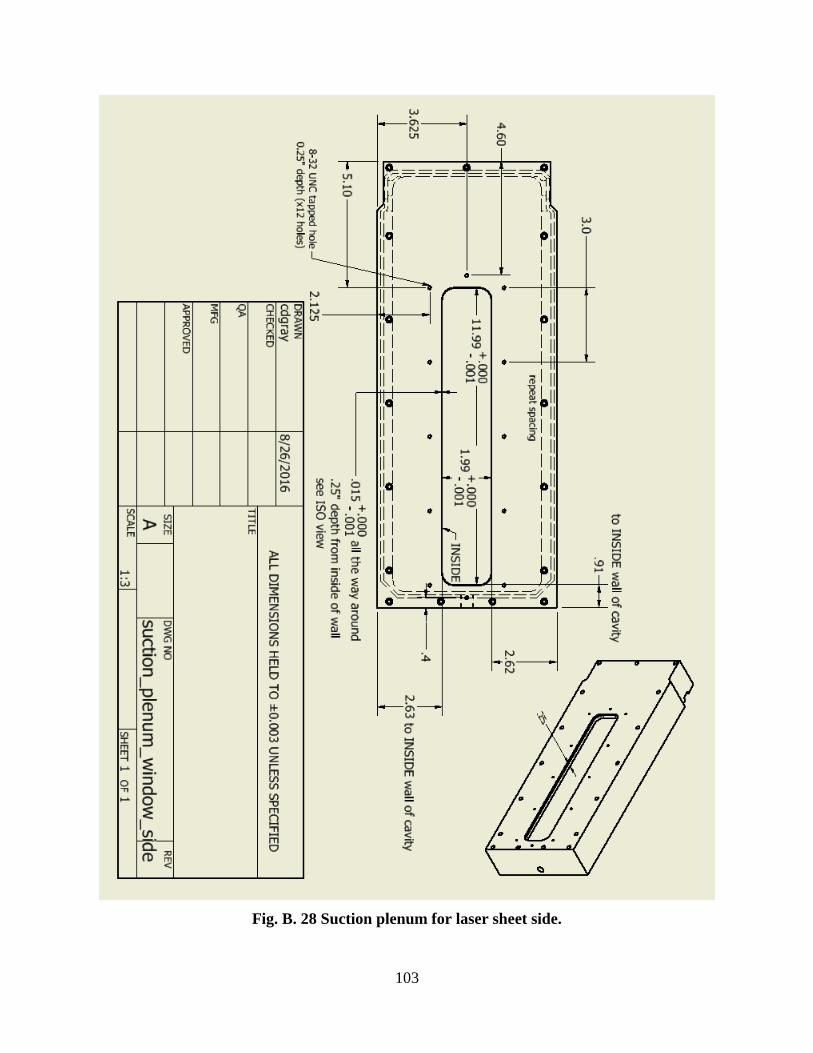
103

Fig. B. 28 Suction plenum for laser sheet side.

104

References

1 Goethert, B.H., “Transonic Wind Tunnel Testing,” Dover, 2007. 2 Anderson, J.D., “Modern Compressible Flow With Historical Perspectives,” 3rd Edition,

McGraw-Hill Companies, Inc., New York, 2003. 3 Mason, W.H., “Transonic Aerodynamics of Airfoils and Wings,” 2006. 4 Wright, R.H. and Ward, V.G., “NACA Transonic Wind-Tunnel Test Sections,” NACA Technical

Report 1231, 1955. 5 Pope, A. and Goin, K.L., High-Speed Wind Tunnel Testing, John Wiley and Sons, Inc., 1965.

6 Vukasinovic, B., Gissen, A.N., Glezer, A., and Gogineni, S., “Fluidic Control of Transonic

Shock-Induced Separation,” AIAA Paper 2013-0529, 2013. 7 AirPro Fan & Blower Company, https://airprofan.com 8 Goett, H.J., “Experimental Investigation of the Momentum Method for Determining Profile

Drag,” NACA Report No. 660, 1939.

9 Batill, S.M. and Hoffman, J.J., “Aerodynamic Design of High Contraction Ratio, Subsonic Wind

Tunnel Inlets,” AIAA Paper 84-0416, 1984. 10 Batill, S.M., Caylor, M.J., and Hoffman, J.J., “An Experimental and Analytic Study of the Flow

in Subsonic Wind Tunnel Inlets,” AFWAL-TR-83-3109, 1983. 11 Derbunovich, G.I., Zemskaya, A.S., Repik, E.U., and Sosedko, Y.P., “Optimum Conditions of

Turbulence Reduction With Screens,” 1991. 12 Dryden, H.L. and Schubauer, G.B., “The Use of Damping Screens for the Reduction of Wind-

Tunnel Turbulence,” Journal of Aeronautical Sciences, 1947. 13 Prandtl, L., “Attaining a Steady Air Stream in Wind Tunnels,” National Advisory Committee

forAeronautics, Technical Memorandum No. 726, 1933. 14 Kulkarni, V., Sahoo, N., and Chavan, S.D., “Simulation of honeycomb-screen combinations for

turbulence management in a subsonic wind tunnel,” Journal of Wind Engineering and Industrial

Aerodynamics, Vollume 99, Issue 1, 2011. 15 Loehrke, R. I. and Nagib, H.M., “Control of Free-Stream Turbulence by Means of Honeycombs:

A Balance Between Suppression and Generation,” ASME, 1976. 16 Eckert, W.T., Mort, K.W., and Jope, J. “Aerodynamic Design Guidelines and Computer

Program for Estimation of Subsonic Wind Tunnel Performance,” NASA TN D-8243, 1976.

105

17 Mehta, R.D. and Bradshaw, P., “Design Rules for Small Low Speed Wind Tunnels,” The

Aeronautical Journal, November 1979. 18 Mehta, R.D., “Turbulent Boundary Layer Perturbed by a Screen,” AIAA Journal, Vol. 23 No.9,

1985. 19 Mehta, R.D., “The Aerodynamic Design of Blower Tunnels with Wide-Angle Diffusers,” Prog.

Aerospace Sci., Vol. 18, pp. 59-120, 1977. 20

Barlow, J.B., Rae, W.H. Jr. and Pope, A., “Low-Speed Wind Tunnel Testing,” 3rd Edition, John

Wiley & Sons, Inc., New York, 1999. 21 “Strength/Mechanics of Materials,” www.engineersedge.com, 2000. 22 Vos, R. and Farokhi, S., Introduction to Transonic Aerodynamics, Springer, 2015. 23 Tokaty, G.A., Fluid Dynamics, W & J Mackay & Co., 1971. 24 Chew, W.L., “Wind Tunnel Investigations of Transonic Test Sections- Phase II: Comparison of

Results of Test of Five Perforated-Wall Test Sections in Conjunction with a Sonic Nozzle,”

AEDC-TR-54-52, 1955. 25 Holder, D.W., North R.D., and Chinneck, A., “Experiments with Slotted and Perforated Walls

in a Two-dimensional High-Speed Tunnel,” T.P.352 F.M. 1631, 1951.