Embed Size (px)
Citation preview

Design and Data Analysis in Psychology I
Salvador Chacón MoscosoSusana Sanduvete Chaves
School of PsychologyDpt. Experimental Psychology
1

Lesson 11
Relationship between two quantitative variables
2

INTRODUCTION When assumptions are accepted
(parametric tests): Simple linear regression (it is going to be
studied next academic year in the subject Design and Data Analysis in Psychology II).
Pearson correlation.
When assumptions are not accepted (non-parametric tests): Spearman correlation.
3

PEARSON CORRELATION: DEFINITION
• rXY
• Coefficient useful to measure covariation between variables: in which way changes in a variable are associated to the changes in other variable.
• Quantitative variables (interval or ratio scale).• Linear relationship EXCLUSIVELY.• Values: -1 ≤ rXY ≤ +1.• Interpretation:
+1: perfect positive correlation (direct association).-1: perfect negative correlation (inverse association).0: no correlation.
4

5
Perfect positive correlation: rxy = +1 (difficult to find in psychology)

6
Positive correlation: 0 < rxy < +1

7
Perfect negative correlation: rxy = -1 (difficult to find in psychology)

8
Negative correlation: -1 < rxy < 0

9
No correlation

Formulas
10
YXXY SS
YXN
XY
r
22 yx
xyrXY
N
ZZr YXXY
Raw scores
Deviation scores
Standard scores

ExampleX: 2 4 6 8 10 12 14 16 18 20 Y:1 6 8 10 12 10 12 13 10 22
1. Calculate rxy in raw scores.
2. Calculate rxy in deviation scores.
3. Calculate rxy in standard scores.
11

Example: scatter plot
12

Example :calculation of rxy in raw scores
X Y XY X2 Y2
2 1 2 4 14 6 24 16 366 8 48 36 648 10 80 64 10010 12 120 100 14412 10 120 144 10014 12 168 196 14416 13 208 256 16918 10 180 324 10020 22 440 400 484110 104 1390 1540 1342
13

Example :calculation of rxy in raw scores
14
839.0103.5*745.5
4.10*1110
1390
YXXY SS
YXN
XY
r
1110
110
N
XX
4.1010
104
N
YY
745.51110
1540 222
XN
XSx
103.54.1010
1342 222
YN
YS y

Example :calculation of rxy in deviation scores
X Y x y xy x2 y2
2 1 -9 -9.4 84.6 81 88.364 6 -7 -4.4 30.8 49 19.366 8 -5 -2.4 12 25 5.768 10 -3 -0.4 1.2 9 0.1610 12 -1 1.6 -1.6 1 2.5612 10 1 -0.4 -0.4 1 0.1614 12 3 1.6 4.8 9 2.5616 13 5 2.6 13 25 6.7618 10 7 -0.4 -2.8 49 0.1620 22 9 11.6 104.4 81 134.56110 104 0 0 246 330 260.4
15
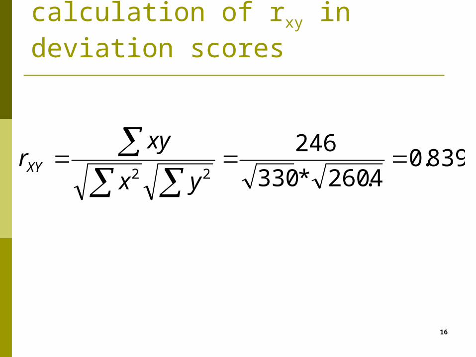
Example :calculation of rxy in deviation scores
16
839.04.260*330
24622
yx
xyrXY

Example :calculation of rxy in standard scores
X Y Zx Zy ZxZy2 1 -1.567 -1.842 2.8864 6 -1.218 -0.862 1.0516 8 -0.870 -0.470 0.4098 10 -0.522 -0.078 0.04110 12 -0.174 0.314 -0.05512 10 0.174 -0.078 -0.01414 12 0.522 0.314 0.16416 13 0.870 0.510 0.44318 10 1.218 -0.078 -0.09620 22 1.567 2.273 3.561110 104 0 0 8.391
17

Example :calculation of rxy in standard scores
18
839.010
391.8
N
ZZr YXXY
XX S
XXZ
YY S
YYZ

Significance
Does the correlation coefficient show a real relationship between X and Y, or is that relationship due to hazard?
Null hypothesis H0: rxy = 0. The correlation coefficient is drawn from a population whose correlation is zero (ρXY = 0).
Alternative hypothesis H1: . The correlation coefficient is not drawn from a population whose correlation is different to zero (ρXY ).
19
0XYr
0
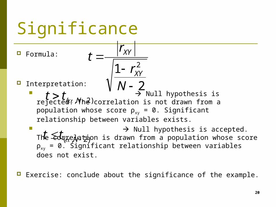
Significance Formula:
Interpretation: Null hypothesis is rejected. The
correlation is not drawn from a population whose score ρxy = 0. Significant relationship between variables exists.
Null hypothesis is accepted. The correlation is drawn from a population whose score ρxy = 0. Significant relationship between variables does not exist.
Exercise: conclude about the significance of the example.20
21 2
Nr
rt
XY
XY
)2,( Ntt
)2,( Ntt
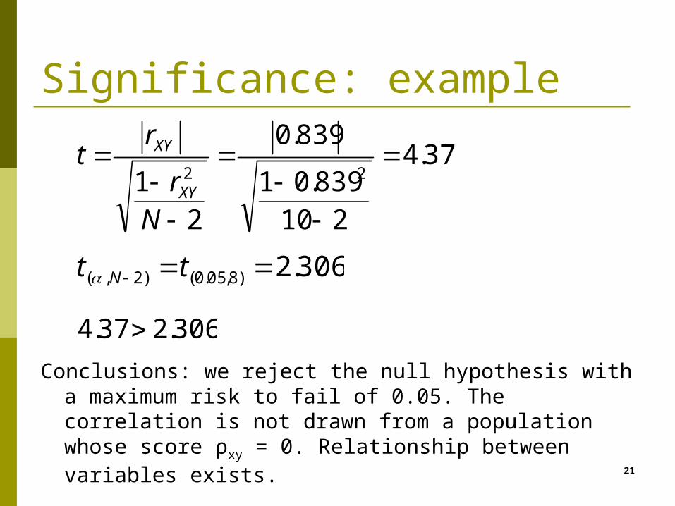
Significance: example
Conclusions: we reject the null hypothesis with a maximum risk to fail of 0.05. The correlation is not drawn from a population whose score ρxy = 0. Relationship between variables exists. 21
37.4
210839.01
839.0
21 22
Nr
rt
XY
XY
306.2)8,05.0()2,( tt N
306.237.4

Other questions to be considered Correlation does not imply causality. Statistical significance depends on sample size (higher N,
likelier to obtain significance). Other possible interpretation is given by the coefficient of
determination , or proportion of variability in Y that is ‘explained’ by X.
The proportion of Y variability that left unexplained by X is called coefficient of non-determination:
Exercise: calculate the coefficient of determination and the coefficient of non-determination and interpret the results.
22
2XYr
21 XYr

Coefficient of determination: example
70.4% of variability in Y is explained by X.
29.6% of variability in Y is not explained.
23
704.0839.0 22 XYr
296.0839.011 22 XYr

Which is the final conclusion?
Significant effect
Non-significant effect
High effect size (≥ 0.67)
The effect probably exists
The non-significance can be
due to low statistical power
Low effect size (≤ 0.18)
The statistical significance can be due to an excessive
high statistical power
The effect probably does not exist
24

Which is the final conclusion?
Significant effect
Non-significant effect
High effect size (≥ 0.67)
The effect probably exists
The non-significance can be
due to low statistical power
Low effect size (≤ 0.18)
The statistical significance can be due to an excessive
high statistical power
The effect probably does not exist
25


![[Moscoso GarcÃ-A, Francisco] Cuentos en Dialecto Ã(BookFi.org)](https://img.pdfslide.us/doc/110x75/55cf8efa550346703b97ad07/moscoso-garca-a-francisco-cuentos-en-dialecto-abookfiorg.jpg)