Design and Construction Procedures forConcrete Overlay and Widening of Existing

Pavements

Final ReportSeptember 2005

Sponsored by Federal Highway Administration (Project 6)

and the Iowa Highway Research Board (Project TR-511)

Disclaimer Notice

The opinions, findings, and conclusions expressed in this publication are those of the authors and not necessarily those of the Federal Highway Administration, Iowa Highway Research Board, or Iowa Department of Transportation. The sponsors assume no liability for the contents or use of the information contained in this document. This report does not constitute a standard, specifica-tion, or regulation. The sponsors do not endorse products or manufacturers.

The contents of this report reflect the views of the authors, who are responsible for the facts and the accuracy of the information presented herein. This document is disseminated under the sponsorship of the U.S. Department of Transportation in the interest of information exchange. The U.S. Government assumes no liability for the contents or use of the information contained in this document. This report does not constitute a standard, specification, or regulation.

The U.S. Government does not endorse products or manufacturers. Trademarks or manufactur-ers’ names appear in this report only because they are considered essential to the objective of the document.

About the PCC Center/CTRE

The Center for Portland Cement Concrete Pavement Technology (PCC Center) is housed at the Center for Transportation Research and Education (CTRE) at Iowa State University. The mission of the PCC Center is to advance the state of the art of portland cement concrete pavement tech-nology. The center focuses on improving design, materials science, construction, and mainte-nance in order to produce a durable, cost-effective, sustainable pavement.

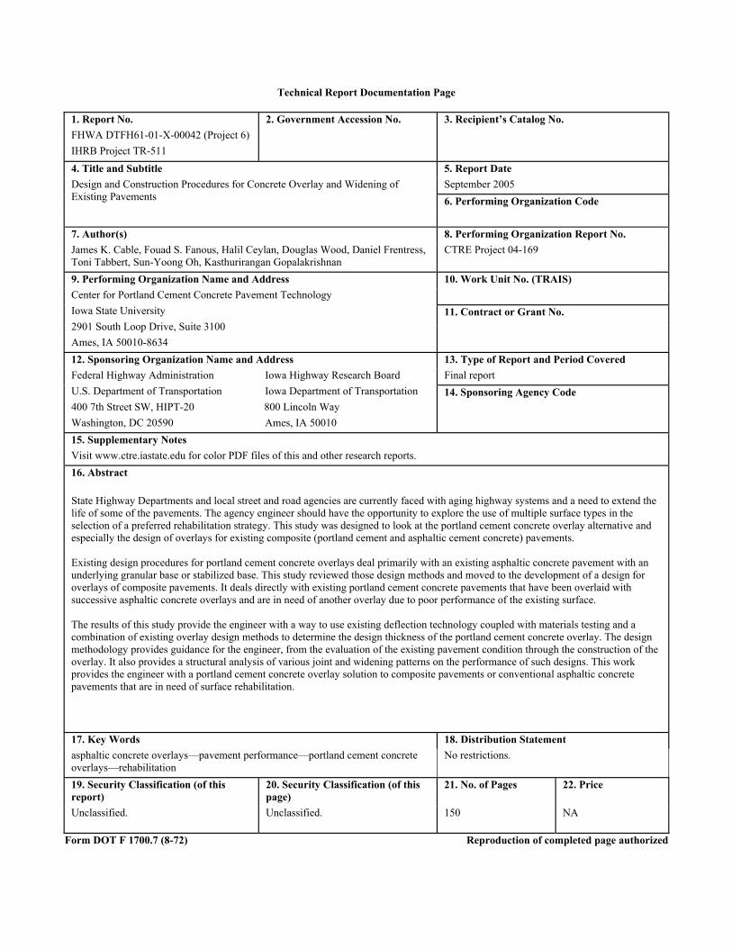
Technical Report Documentation Page

1. Report No. FHWA DTFH61-01-X-00042 (Project 6) IHRB Project TR-511

2. Government Accession No. 3. Recipient’s Catalog No.

4. Title and Subtitle Design and Construction Procedures for Concrete Overlay and Widening of Existing Pavements

5. Report Date September 2005 6. Performing Organization Code

7. Author(s) James K. Cable, Fouad S. Fanous, Halil Ceylan, Douglas Wood, Daniel Frentress, Toni Tabbert, Sun-Yoong Oh, Kasthurirangan Gopalakrishnan

8. Performing Organization Report No. CTRE Project 04-169

9. Performing Organization Name and Address Center for Portland Cement Concrete Pavement Technology Iowa State University 2901 South Loop Drive, Suite 3100 Ames, IA 50010-8634

10. Work Unit No. (TRAIS)

11. Contract or Grant No.

12. Sponsoring Organization Name and Address Federal Highway Administration Iowa Highway Research Board U.S. Department of Transportation Iowa Department of Transportation 400 7th Street SW, HIPT-20 800 Lincoln Way Washington, DC 20590 Ames, IA 50010

13. Type of Report and Period Covered Final report 14. Sponsoring Agency Code

15. Supplementary Notes Visit www.ctre.iastate.edu for color PDF files of this and other research reports. 16. Abstract

State Highway Departments and local street and road agencies are currently faced with aging highway systems and a need to extend the life of some of the pavements. The agency engineer should have the opportunity to explore the use of multiple surface types in the selection of a preferred rehabilitation strategy. This study was designed to look at the portland cement concrete overlay alternative and especially the design of overlays for existing composite (portland cement and asphaltic cement concrete) pavements.

Existing design procedures for portland cement concrete overlays deal primarily with an existing asphaltic concrete pavement with an underlying granular base or stabilized base. This study reviewed those design methods and moved to the development of a design for overlays of composite pavements. It deals directly with existing portland cement concrete pavements that have been overlaid with successive asphaltic concrete overlays and are in need of another overlay due to poor performance of the existing surface.

The results of this study provide the engineer with a way to use existing deflection technology coupled with materials testing and a combination of existing overlay design methods to determine the design thickness of the portland cement concrete overlay. The design methodology provides guidance for the engineer, from the evaluation of the existing pavement condition through the construction of the overlay. It also provides a structural analysis of various joint and widening patterns on the performance of such designs. This work provides the engineer with a portland cement concrete overlay solution to composite pavements or conventional asphaltic concrete pavements that are in need of surface rehabilitation.

17. Key Words asphaltic concrete overlays—pavement performance—portland cement concrete overlays—rehabilitation

18. Distribution Statement No restrictions.

19. Security Classification (of this report) Unclassified.

20. Security Classification (of this page) Unclassified.

21. No. of Pages

150

22. Price

NA

Form DOT F 1700.7 (8-72) Reproduction of completed page authorized

DESIGN AND CONSTRUCTION PROCEDURES FOR CONCRETE OVERLAY AND WIDENING OF

EXISTING PAVEMENTS

Final Report September 2005

Principal Investigator James K. Cable

Associate Professor Department of Civil, Construction and Environmental Engineering, Iowa State University

Co-Principal Investigators Fouad S. Fanous

Professor Department of Civil, Construction and Environmental Engineering, Iowa State University

Halil CeylanAssistant Professor

Department of Civil, Construction and Environmental Engineering, Iowa State University

Research Associates Douglas Wood, Daniel Frentress, Kasthurirangan Gopalakrishnan

Research Assistants Toni Tabbert, Sun-Yoong Oh

Sponsored by the Federal Highway Administration (Project 6) andthe Iowa Highway Research Board (Project TR-511)

Preparation of this report was financed in part through funds provided by the Iowa Department of Transportation

through its research management agreement with the Center for Transportation Research and Education

CTRE Project 04-169

Center for Portland Cement Concrete Pavement Technology Iowa State University

2901 South Loop Drive, Suite 3100 Ames, IA 50010-8634 Phone: 515-294-8103 Fax: 515-294-0467

www.pcccenter.iastate.edu

TABLE OF CONTENTS

ACKNOWLEDGMENTS ............................................................................................................ IX

INTRODUCTION ...........................................................................................................................1

Objectives................................................................................................................................... 1 Research Plan............................................................................................................................. 2

PART I—ANALYTICAL STUDIES AND FIELD TESTING ......................................................4

Background ................................................................................................................................ 4 Objectives................................................................................................................................... 6 Approach.................................................................................................................................... 6 Literature Review....................................................................................................................... 7

Analytical Studies ................................................................................................................. 7 Finite Element Modeling Techniques for Composite Pavements ......................................... 8

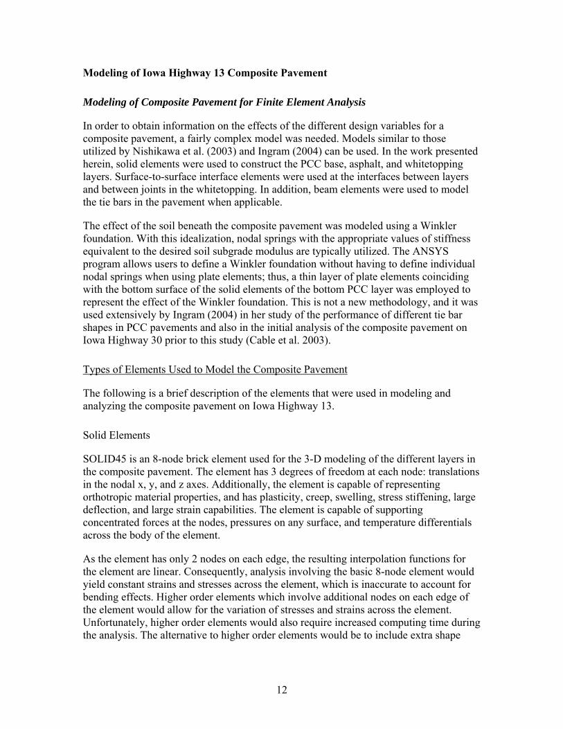
Modeling of Iowa Highway 13 Composite Pavement ............................................................. 12 Modeling of Composite Pavement for Finite Element Analysis......................................... 12 Verification of ANSYS Model............................................................................................ 18

Field Investigation of Iowa Highway 13 Composite Pavement............................................... 19 Field Test............................................................................................................................. 19 Composite Pavement Analysis with Field Test Loads........................................................ 24

Analysis of Iowa Highway 13 Composite Pavement............................................................... 31 Parametric Study of Composite Pavement.......................................................................... 31 Pavement Behavior When Subjected to Truck Loading ..................................................... 40 Pavement Behavior When Subjected to Temperature Differential ..................................... 43

PART II—OVERLAY DESIGN METHODOLOGY...................................................................47

Literature Review of Existing Methods ................................................................................... 47 ACPA/PCA Ultra-Thin Whitetopping Design Guidelines.................................................. 47 Colorado Thin Whitetopping Design Procedure................................................................. 52 Illinois (Riley et al. 2005) ................................................................................................... 59 Transtec Overlay Design..................................................................................................... 62

Mechanistic Whitetopping Thickness Design Procedure ........................................................ 71 Evaluation of the Existing Pavement ....................................................................................... 71

Temperature Effects ............................................................................................................ 71 Asphalt Modulus ................................................................................................................. 71 Backcalculation of the Subgrade K-Value and Concrete Modulus..................................... 72 PCC Elastic Modulus .......................................................................................................... 75

Effective Thickness of Existing Pavement .............................................................................. 75 Effective “Plate” Theory ..................................................................................................... 75 Unbonded ACC and PCC Layer ......................................................................................... 76 Bonded ACC and PCC Layers ............................................................................................ 76

Design Implementation ............................................................................................................ 77 Iowa 175.............................................................................................................................. 77

v

Overlay Planning Guidelines ................................................................................................... 78 Overlay Design Guidelines ...................................................................................................... 80 Overlay Construction Guidelines............................................................................................. 82

SUMMARY, CONCLUSIONS, AND RECOMMENDATIONS.................................................85

Analytical study ....................................................................................................................... 85 Summary ............................................................................................................................. 85 Conclusions ......................................................................................................................... 86 Future Recommendations.................................................................................................... 87

REFERENCES ..............................................................................................................................89

APPENDIX A: STRAIN GAGE DATA .................................................................................... A-1

APPENDIX B: IOWA 175 DESIGN EXAMPLE.......................................................................B-1

vi

LIST OF FIGURES

Figure 1. Schematics of the composite pavement (not to scale).........................................................5 Figure 2. 3-D finite element model (Wu et al. 1998)........................................................................10 Figure 3. Interface elements (Nishizawa et al. 2003) .......................................................................11 Figure 4. Orientation of interface element ........................................................................................14 Figure 5. Friction model ...................................................................................................................15 Figure 6. Finite element model details (not to scale)........................................................................16 Figure 7. Location of tie bars (not to scale) ......................................................................................17 Figure 8. Sample composite pavement model ..................................................................................18 Figure 9. Schematic of FWD deflection sensors ..............................................................................19 Figure 10. Temperature and strain gages along Iowa highway 13 ...................................................21 Figure 11. Configuration of truck load used for strain data collection.............................................22 Figure 12. Test truck provided by IDOT for strain data collection ..................................................22 Figure 13. Example of strain gage reading .......................................................................................23 Figure 14. Example of composite pavement deflected shape (9-kip load) (plan view—

exaggerated scale).................................................................................................................25 Figure 15. Example of composite pavement deflected shape (9-kip load) (cross-section view—

exaggerated scale).................................................................................................................25 Figure 16. Deflection comparison for pavement with 3.5″ whitetopping and 4.5 ft joint spacing...26 Figure 17. Deflection comparison for pavement with 3.5″ whitetopping and 6 ft joint spacing......26 Figure 18. Deflection comparison for pavement with 3.5″ whitetopping and 9 ft joint spacing......27 Figure 19. Deflection comparison for pavement with 4.5″ whitetopping and 4.5 ft joint spacing...27 Figure 20. Deflection comparison for pavement with 4.5″ whitetopping and 6 ft joint spacing......28 Figure 21. Deflection comparison for pavement with 4.5″ whitetopping and 9 ft joint spacing......28 Figure 22. Comparison of experimental and analytical strain results...............................................29 Figure 23. Deflection profiles for pavements with 3.5″ and 4.5″ whitetopping thickness ...............32 Figure 24. Comparison of deflections for bonded layers and unbonded layers................................35 Figure 25. Maximum deflections—varying widening unit widths (9-kip load)...............................37 Figure 26. Maximum deflections—varying widening unit depths (9-kip load) ...............................37 Figure 27. Insertion of interface elements between widening unit and composite section ..............38 Figure 28. Separation at widening unit–composite section interface (cross-section view—

exaggerated scale).................................................................................................................39 Figure 29. Partial separation at widening unit–composite section interface (cross-section view—

exaggerated scale).................................................................................................................40 Figure 30. Location of truck outer wheel on composite pavement...................................................41 Figure 31. Configuration of truck loads with two lanes loaded........................................................42 Figure 32. Temperature differentials applied to the composite pavement........................................44 Figure 33. Schematic of framework to optimizing whitetopping design (The Transtec Group

2005) .....................................................................................................................................63 Figure 34. Ida county site map..........................................................................................................77 Figure 35. Sac county site map .........................................................................................................77

vii

LIST OF TABLES

Table 1. Breakdown of maximum deflection data from FWD test: 3.5″ whitetopping pavement ......20 Table 2. Breakdown of maximum deflection data from FWD test: 4.5″ whitetopping pavement ......20 Table 3. Maximum composite pavement deflections (9-kip load) ......................................................32 Table 4. Maximum transverse stresses (psi) for different joint configurations (9-kip load) ...............32 Table 5. Maximum longitudinal stresses (psi) for different joint configurations (9-kip load) ............33 Table 6. Maximum deflections due to varying overlay crack depths (9-kip load) ..............................34 Table 7. Maximum stresses (psi) for full overlay depth joint cracks (9-kip load)...............................34 Table 8. Maximum transverse stresses (psi) for bonded/unbonded composite pavement (9-kip

load) .........................................................................................................................................35 Table 9. Maximum longitudinal stresses (psi) for bonded/unbonded composite pavement (9-kip

load) .........................................................................................................................................36 Table 10. Maximum deflection and stresses in the composite pavement (single truck load) .............41 Table 11. Maximum deflection and stresses in the composite pavement (double truck load) ............42 Table 12. Maximum deflection and stresses due to worst case loading of the composite pavement ..43 Table 13. Maximum deflections and whitetopping–ACC interface stresses (temperature

differential) ..............................................................................................................................45 Table 14. Maximum transverse stresses in the composite pavement (temperature differential).........45 Table 15. Maximum longitudinal stresses in the composite pavement (temperature differential)......45 Table 16. Comparison of whitetopping design procedures .................................................................69 Table B.1. Iowa 175 input parameters ...............................................................................................B-2 Table B.2. Eastbound lane backcalculation of layer parameters .......................................................B-3 Table B.2a. Bonded layer condition (eastbound lane).......................................................................B-6 Table B.2b. Unbonded layer conditions (eastbound lane).................................................................B-9 Table B.3. CDOT whitetopping thickness for 20-year traffic prediction (bonded–eastbound

lane)......................................................................................................................................B-13 Table B.4. CDOT whitetopping thickness for 20-year traffic prediction (unbonded–eastbound

lane)......................................................................................................................................B-15 Table B.5. PCA whitetopping thickness for 20-year traffic prediction (bonded–eastbound lane)..B-17 Table B.6. PCA whitetopping thickness for 20-year traffic prediction (unbonded–eastbound

lane)......................................................................................................................................B-19 Table B.7. Westbound lane backcalculation of layer parameters....................................................B-21 Table B.7a. Bonded layer condition (westbound lane)....................................................................B-24 Table B.7b. Unbonded layer condition (westbound lane) ...............................................................B-26 Table B.8. CDOT whitetopping thickness for 20-year traffic prediction (bonded–westbound

lane)......................................................................................................................................B-29 Table B.9. CDOT whitetopping thickness for 20-year traffic prediction (unbonded–westbound

lane)......................................................................................................................................B-31 Table B.10. PCA whitetopping thickness for 20-year traffic prediction (bonded–westbound

lane)......................................................................................................................................B-33 Table B.11. PCA whitetopping thickness for 20-year traffic prediction (unbonded–westbound

lane)......................................................................................................................................B-35

viii

ACKNOWLEDGMENTS

The project research staff wants to thank Iowa DOT and Manchester Maintenance Garage staff for their support in the conduct of the field strain and pavement temperature testing. The traffic control equipment was essential to the installation and testing done for this project.

ix

INTRODUCTION

Iowa is currently one of the few states with two thin PCC overlay projects in place that are in excess of one mile in length. The first of these pavement overlays was placed in 1994 and has been used to investigate the optimum overlay for asphaltic concrete base pavements. The second pavement overlay was placed in 2002 and focused on additional investigation of the overlay depth and the impact of fibers and pavement widening on the pavement performance. These projects have proved that thin overlays are capable of becoming an alternative to asphaltic concrete overlays.

As a result of the previous work in Iowa, a need for a design manual for the engineer to use in the selection of pavement rehabilitation candidates for PCC widening and overlay projects was identified. This project was also envisioned to move the research results of the existing PCC overlay research in Iowa and nationally into an implementation mode.

This research also sought to answer some of the current issues in PCC overlay construction:

1. Selection criteria for implementation of successful PCC overlays, such as traffic needs, climate, underlying pavement condition, and depth of each pavement layer.

2. Traffic control requirements for various traffic volumes and mixes of vehicles. 3. Consideration of single lane paving techniques. 4. Design relationships:

a. Traffic volume and mix vs. overlay depth b. Widening depth and width vs. structural enhancement of overlay c. Structural evaluation of underlying pavement vs. overlay depth d. Fiber contribution vs. overlay performance. e. Need for widening tie bars, size, spacing, and method of placement.

5. Design and performance of the stress reliever layer materials, surface texture, and bonding capability.

6. Structural evaluation of the impact of the widening unit and the joint spacing of the overlay on the long-term performance of the pavement.

Objectives

The objectives of this research focused on four areas:

1. Conduct of a structural analysis of the overlay and widening unit contributions to stress reductions and extended pavement life of the composite pavement.

2. Development of construction guidelines for construction of thin concrete overlays and widening units and a catalog of designs employed.

3. Development of an overlay design procedures for thin PCC overlays and widening units.

4. Validation of the structural analysis and design procedure with field load tests and strain measures for the various pavement layers of the existing two material/layer pavements.

1

Research Plan

The research was carried out using the two Iowa PCC overlay projects as a basis for analysis of the performance of various design components. Those pavements included the Iowa Highway 21 (7.2 mile) section from U.S. Highway 6 north to Iowa Highway 212 and the Iowa Highway 13 project from Manchester north to the junction of Iowa Highway 3.

A finite element computer analysis coupled with field strain gage installation was used for the structural analysis. The details of the field installation and the results are shown in Part I of this report.

Individual parts of the project were subdivided into the following tasks:

Task 1. Structural Analysis

1. Field evaluation and validation of strain measures in two existing overlay research pavements in Iowa to validate the current finite element results for the unbonded overlays.

2. Enhancement of previous structural analysis of the various overlay joint patterns and widening unit combinations of depth vs. width impact on the stress/strain imparted to the underlying pavement layers and life of the overlay.

3. Evaluation of the impact of the reinforcement ties between the widening unit and the overlay to include the following:

a. Slab sizes, including, but not limited to 2x2, 4x4, 4.5x4, 5x5, 5.5x5.5, 6x6, 9x9, 10x10, 11x11, 12x12, and 12x15 feet.

b. Overlay depths of 2, 3.5, 4, 4.5, and 6 inches. c. Widening unit, varying in width from 1 ft. to 5 ft. in one-foot

increments in conjunction with a constant depth of 8 inches.

Task 2. Development of guidelines for the selection of candidate projects for PCC overlays

1. Structural and visual evaluation of the existing pavement layers. 2. Estimation of the future traffic needs. 3. Evaluation of traffic control needs during construction.

Task 3. Development of draft design guidelines for the overlay and widening units

1. Design of depth and width to meet traffic needs and control. 2. Use of fibers and widening tie methods. 3. Design of widening units, overlay joint spacing, and widening connection to

existing pavements.

Task 4. Innovation

1. Consideration of new paving techniques to enhance pavement overlay construction and/or reduce traffic control problems during construction.

2

2. Consideration of new ways to introduce fibers into the mix. 3. Consideration of new joint forming methods to reduce construction time. 4. Consideration of design applications to bus loading areas and intersections or

parking lots.

Task 5. Demonstration and validation

1. Development of a demonstration project or projects to illustrate the results of the research.

2. Validation of the results of the structural design enhancements with a field demonstration project.

3. Development of the project report and implementation presentations. 4. Evaluation of the resulting field demonstration project after one year.

The work was divided into two major areas of structural analysis and design process development. These are reported on in the same order in the following portions of the report.

3

PART I—ANALYTICAL STUDIES AND FIELD TESTING

Background

Resurfacing hot mix asphalt (HMA) pavements with thin Portland Cement Concrete (PCC) overlays, or “whitetopping” as it has come to be known, is a concept that dates back to 1918. This approach has seen a large increase in use in the past 15 years due to improved whitetopping technology and the success of several high-profile projects (NCHRP 2002). Whitetopping provides several advantages to the conventional resurfacing of pavements with HMA. It significantly reduces time and delays associated with pavement maintenance utilizing asphalt. PCC surfaces also have proven durability and long-term performance, which allows for longer life at lower life-cycle costs as compared to asphalt surfaces (Burnham and Rettner 2003).

The state of Iowa is one of several states known for the large amount of PCC pavements. The original design life of the initial pavement systems was established as 20 years, and most of the systems had reached or exceeded the design life by the 1970s. These pavements were then continually resurfaced and possibly widened with asphalt cement concrete (ACC) to extend the life for another 10 to 15 years or until funding could be obtained to replace the pavements (Cable et al. 2003; Burnham and Rettner 2003). Due to the shorter design life and higher maintenance costs of asphalt pavements throughout that design life, whitetopping presents an attractive, lower cost alternative to continued pavement rehabilitation of asphalt surfaces.

In 1994, the Iowa Department of Transportation (Iowa DOT) initiated an ultra-thin whitetopping (UTW) project on a 7.2-mile segment of Iowa Highway 21 in Iowa County, near Belle Plaine, Iowa. The objective of that research was to investigate the interface bonding condition between an ultra-thin PCC overlay and an ACC base over time, with consideration given to the combination of different factors, such as ACC surface preparation, PCC thickness, the usage of synthetic fiber reinforcement, joint spacing, and joint sealing. That research continues to be one of the most referenced in demonstrating the applicability of whitetopping as a viable rehabilitation option.

In 2002, a follow-up project was initiated by Iowa DOT to investigate and verify the findings from the 1994 study (Cable et al. 2003). For this purpose, a 9.6-mile long stretch of Iowa Highway 13 (IA 13) that extends from Manchester, Iowa, to Iowa Highway 3 in Delaware County was selected as the test site. The pavement section consisted of a bottom PCC layer constructed in 1931 that was 18 ft wide, with a thickened edge that is 10″ at the edges and 7″ at the centerline of the roadway. The concrete pavement was used as the driving surface until subsequently overlaid with 2″ of asphalt concrete in 1964 and with another asphalt concrete overlay of 3″ in 1984.

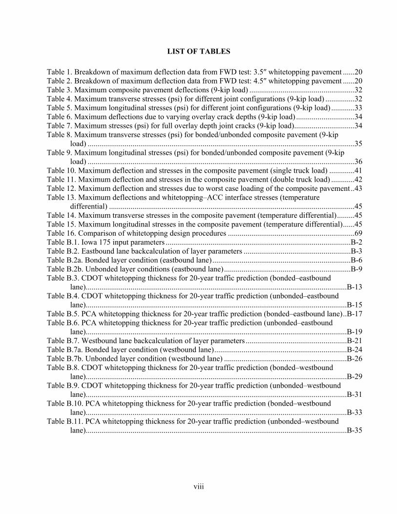
Whitetopping was utilized in the summer of 2002 to rehabilitate the Iowa Highway 13 roadway and was applied considering the following variables: ACC surface preparation (milled, one-inch HMA stress relief course, and broomed only); use of fiber reinforcement in concrete (polypropylene, monofilament, proprietary structural, and no

4

fibers); joint spacing (4.5 x 4.5, 6 x 6, and 9 x 9-foot sections); and joint/crack preparation (bridge with concrete or #4 rebars stapled to the asphalt surface). The pavement section was also widened during the overlay operation to its current 24 ft width. The details of the construction were presented in a separate construction report presented by the Center for Portland Cement Concrete Pavement Technology at Iowa State University (Cable et al. 2003).

9’ 9’

9 9’ 9’

4.5’ 4.5’ 4.5’ 4.5’ 5’ 5’

6’

6’

6’ 6’

4.5’ 4.5’

6’. 6’

Joint formed not sawed (1.5” deep) Sawed joints (1.5” deep)

(a) Plan – Various joint spacing configuration

5’ 9’ 9’ 5’

5”7”

5”

PCC

ACC PCC

Concrete Concrete

3.5” or 4.5”

10” 8”

10”10”

Widening 18’ Composite Section’ Widening Unit

(b) Pavement cross-section Unit

Figure 1. Schematics of the composite pavement (not to scale)

The construction report also included an analytical study utilizing the finite element method to predict the behavior of the composite pavement under truck loads. Several observations on the overall structural behavior of the pavement were made with regards to factors such as variation of soil subgrade reaction values, pavement cross-slope, and joint crack depth. The widening units were also found to be beneficial to pavement performance by reducing deflection and stresses. However, the state of bonding between

5

the layers, the different joint spacings, the effect of the rebars, and the effect of temperature variation were not part of the investigation (Cable et al. 2003).

The study presented herein is an extension of the initial analytical work presented in the construction report (Cable et al. 2003) and is focused on analytically investigating the factors that were not studied in the aforementioned analytical work.

Objectives

The objectives of the study presented herein were as follows:

• Develop an analytical model for a finite element analysis that can accurately predict the response of the composite pavement on Iowa Highway 13

• Investigate the behavior of the pavement as whitetopping thickness, joint spacing, and depth of joint cracking was varied

• Examine the effects of bonding between the different layers on the overall structural behavior of the composite pavement

• Investigate the effects of the widening units on the deflection and stresses induced in the composite pavement when subjected to loading

• Determine the effects of bridging the pavement section and widening units with tie bars of different size and spacing

• Investigate the behavior of the pavement when subjected to different thermal conditions

Approach

To achieve the aforementioned objectives, the following tasks were completed:

• Collection of information regarding the dimensions and other considerations about the pavement on Iowa Highway 13

• Determination of the appropriate types of elements for the finite element modeling of the composite pavement. This step required the following:

o Verification of the suitability of interface elements to model the interaction between pavement layers

o Comparison of the results obtained using a general purpose finite element model with those obtained using available specialized pavement analysis software, such as ISLAB2000

o Determination of the appropriate mesh size for the finite element model to ensure accurate results are obtained

• Calibration of the analytical results with field test data on Iowa Highway 13. o Comparison of collected Falling Weight Deflectometer (FWD) test data to

analysis results from pavement subjected to comparable load and ground conditions

o Comparison of measured strain to strain results from the finite element analysis

6

• Analysis of the pavement model with the different design variables under consideration, which include the following:

o Bonded and unbonded layers o Different joint spacing and crack depth o Different widening unit thickness and width o Different rebar bar size and spacing

• Investigation of the behavior of composite pavement under recorded temperature differentials

Literature Review

Analytical Studies

Several analytical methods that range in degree of difficulty from using simple closed form solutions to complex finite element models may be utilized to investigate the performance of composite pavement structures. A three-dimensional (3-D) finite element model for the stress analysis of pavements with UTW was developed as part of a 1997 study of UTW overlays at the Ellaville Weigh Station on I-10 in northern Florida by the Florida DOT. The analysis was an attempt to understand the reason for the poor performance of the UTW sections constructed at the Ellaville Weight Station. The analysis showed that the UTW sections were found to have relatively higher stresses under critical loading conditions, which appeared to explain the poor performance and high incidences of cracked slabs. The 3-D model developed was also used to perform a parametric analysis to determine the effects that various UTW design variables have on performance, such as asphalt thickness, concrete thickness, asphalt and concrete moduli, and subgrade stiffness. The 3-D finite element model was limited by the simplifications of the material behavior to elastic material, full bonding between the layers, and no load transfer between adjacent slabs (thus providing an extreme worst case scenario). Despite these limitations, the project was a valuable demonstration of the applicability of using the finite element method to aid in investigating the performance of whitetopping.

In 1998, the Portland Cement Association (PCA) published a report detailing the development of a first generation design procedure for UTW. The report was based on a comprehensive study involving extensive field load testing, as well as the theoretical evaluation of UTW pavement behavior utilizing 3-D finite element analysis with the NISA II software package (Wu et al. 1998). Field test data was collected from three different sites: from a parking ramp rehabilitation project in the Spirit of St. Louis Airport, constructed in early 1995, and from two whitetopping test sections in Colorado that were instrumented and tested in 1996. Variables such as the slab thickness, joint spacing, joint condition, and asphalt surface preparation were considered in the study. In addition to the development of a rational design procedure for UTW, data collected from these projects have resulted in improved design and construction specifications of the UTW. Among the recommendations of the study were the installation of tie bars along the longitudinal construction joint and avoiding placing whitetopping overlay on top of a newly laid hot mix asphalt (HMA). Subsequent work has supported these findings, but emphasized that

7

the properties of the HMA, whether existing or new, be taken into account in the overlay design (NCHRP 2002).

Analytical work in the PCA study mentioned above also attempted to account for the load transfer between adjacent slabs, as well as the soil support using a system of unidirectional springs. Attempts at modeling the interface bond condition between layers utilizing point-to-point shear-friction gap elements were unsuccessful, and the investigative team subsequently utilized a system of springs to model the interface condition. A finite element program utilizing only shell elements to model pavements— commonly referred to as a 2-D model—was used to perform a parametric analysis, rather than the 3-D model that was developed, in the interests of reducing computational time. Results of the 2-D model were then converted into equivalent 3-D model results by using predictive equations developed from linear regression analysis of results from a control case. Results from the test sections in Colorado were also used in the development of design guidelines for whitetopping by CDOT (Tarr, Sheehan, and Okamoto 1998).

Based upon the premise that the structural design of UTW overlays requires precise predictions of loading stresses in the pavement system, a team of investigators from Tokyo, Japan, developed a 3-D finite element model that takes into account the viscoelastic behavior of asphalt and the interaction between the concrete overlay and asphalt subbase (Nishizawa, Murata, and Kokubun 2003). Analysis was performed on the program Pave3D, which was developed by one of the investigators for the analysis of pavement structures. Loading tests for both stationary and moving loads were conducted on an instrumented test pavement which was constructed in 1999 with two different joint spacings. The measured strains were compared with the computed strains from the finite element model for both stationary and moving loads. The comparison showed that the viscosity of the asphalt subbase and the interface conditions significantly affect the stress behavior of the pavement, affirming qualitative observations in the studies mentioned earlier from an analytical perspective. The study also demonstrated the applicability and advantage of more complex formulations of the finite element method in analyzing the unique behavior of whitetopped composite pavements. However, the report pointed out that precise prediction of stresses at high temperature conditions was still difficult using the 3-D model, even by incorporating viscoelasticity of the asphalt layer.

While attempts at modeling aspects of the more complex behavior of whitetopped pavements have been successful, much effort is still needed to develop a complete model that successfully predicts pavement behavior under a variety of design variables and conditions. However, in the author’s opinion, the seemingly inexhaustible combinations of design variables and project specific considerations, not to mention limited resource availability, may well render this ultimate objective unreachable.

Finite Element Modeling Techniques for Composite Pavements

Two-dimensional finite element programs, such as ISLAB2000 (proprietary revision of ILSL2), J-SLAB, KenPAVE, and FEACONS, have been used in the analysis of pavement systems. These programs are based upon classical theories of analyzing thin plates (also known as medium-thick plates in pavement literature) on Winkler

8

foundations. They have been effectively used to analyze pavements with various slab sizes, different joint conditions, multiple layers, and with linear temperature differentials. However, these software packages do not allow users to model pavements with varying thickness or cross-slopes. Also, representing the configuration of pavements with widened sections would be difficult, if not impossible, when using 2-D finite element models to analyze such a structure; therefore, analysis of a composite pavement, such as the one found on Iowa Highway 13, requires the development of a 3-D model utilizing a general finite element program, such as ABAQUS, ADINA, or ANSYS. The analysis package ANSYS was selected for use in the work presented herein and is presented in detail in chapter “Modeling of Iowa Highway 13 Composite Pavement.”

Modeling of Concrete and Asphalt Layers

Eight-node solid elements, also known as brick elements, can be used to model the concrete and asphalt layers of the composite pavement. Higher order solid elements, i.e., elements with a higher number of nodes, could also be utilized; however, employing higher order elements results in higher requirements for computational resources. To minimize the burden on computational resources and to maintain the accuracy of the finite element results, eight-node brick elements can be utilized by including “extra displacement functions” (Cook et al. 2002). These extra displacement functions are used to correct for the parasitic shear that results from the assumed displacement functions associated with the formulation of the eight-node solid element and allow the element to accurately represent the effects of bending in structures.

Kumara et al. utilized 20-node solid elements to model the UTW pavement layers in their Florida study (2003), whereas Wu et al. (1998) and Nishizawa et al. (2003) utilized the computationally economical eight-node solid element. In the work presented herein, eight-node solid elements with extra displacement functions were utilized in modeling the composite pavement on Iowa Highway 13.

Interface Modeling Techniques

The effect of interface condition is of particular interest in investigating the behavior of the composite pavement, as previous studies have shown that it has a significant effect on the behavior of the whitetopping pavement system. In the analytical work leading to the development of the PCA design procedure for UTW, Wu et al. (1998) attempted to model the interface interaction with the use of non-linear shear-friction gap elements, which were 2-node or point-to-point interface elements that were available with the finite element analysis package NISA II. The element is capable of contact determination between the two layers: “open” or “closed” status. If the interface is “open,” no transfer of loads between the two surfaces occurs. If “closed,” the element resists normal and tangential forces through the use of three orthogonal springs with frictional capabilities in the horizontal direction. The element was capable of allowing sliding at locations where the shear forces exceeded the shear resistance, thereby simulating partial bonding of the pavement layers. Unfortunately, convergence problems in the resulting non-linear solution process forced the investigative team to abandon this approach and, instead, to

9

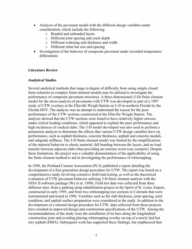
adopt a model that incorporated horizontal spring elements located at the interface of the concrete and asphalt layers. A bonded interface would be associated with very high values of the horizontal spring stiffness and an unbonded interface with very low values. Partially bonded conditions would then be modeled by moderate values of the spring stiffness, which were determined by a trial and error process. The final model adopted by Wu et al. is shown schematically in Figure 2.

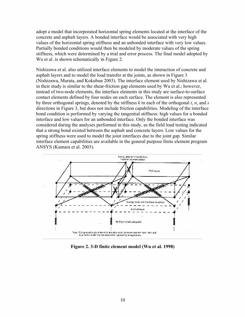
Nishizawa et al. also utilized interface elements to model the interaction of concrete and asphalt layers and to model the load transfer at the joints, as shown in Figure 3 (Nishizawa, Murata, and Kokubun 2003). The interface element used by Nishizawa et al. in their study is similar to the shear-friction gap elements used by Wu et al.; however, instead of two-node elements, the interface elements in this study are surface-to-surface contact elements defined by four nodes on each surface. The element is also represented by three orthogonal springs, denoted by the stiffness k in each of the orthogonal t, n, and s directions in Figure 3, but does not include friction capabilities. Modeling of the interface bond condition is performed by varying the tangential stiffness: high values for a bonded interface and low values for an unbonded interface. Only the bonded interface was considered during the analyses performed in this study, as the field load testing indicated that a strong bond existed between the asphalt and concrete layers. Low values for the spring stiffness were used to model the joint interfaces due to the joint gap. Similar interface element capabilities are available in the general purpose finite element program ANSYS (Kumara et al. 2003).

Figure 2. 3-D finite element model (Wu et al. 1998)

10

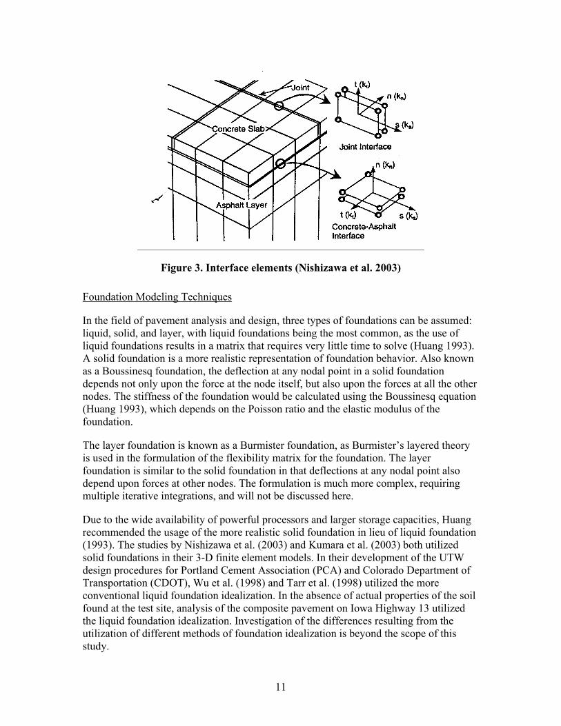
Figure 3. Interface elements (Nishizawa et al. 2003)

Foundation Modeling Techniques

In the field of pavement analysis and design, three types of foundations can be assumed: liquid, solid, and layer, with liquid foundations being the most common, as the use of liquid foundations results in a matrix that requires very little time to solve (Huang 1993). A solid foundation is a more realistic representation of foundation behavior. Also known as a Boussinesq foundation, the deflection at any nodal point in a solid foundation depends not only upon the force at the node itself, but also upon the forces at all the other nodes. The stiffness of the foundation would be calculated using the Boussinesq equation (Huang 1993), which depends on the Poisson ratio and the elastic modulus of the foundation.

The layer foundation is known as a Burmister foundation, as Burmister’s layered theory is used in the formulation of the flexibility matrix for the foundation. The layer foundation is similar to the solid foundation in that deflections at any nodal point also depend upon forces at other nodes. The formulation is much more complex, requiring multiple iterative integrations, and will not be discussed here.

Due to the wide availability of powerful processors and larger storage capacities, Huang recommended the usage of the more realistic solid foundation in lieu of liquid foundation (1993). The studies by Nishizawa et al. (2003) and Kumara et al. (2003) both utilized solid foundations in their 3-D finite element models. In their development of the UTW design procedures for Portland Cement Association (PCA) and Colorado Department of Transportation (CDOT), Wu et al. (1998) and Tarr et al. (1998) utilized the more conventional liquid foundation idealization. In the absence of actual properties of the soil found at the test site, analysis of the composite pavement on Iowa Highway 13 utilized the liquid foundation idealization. Investigation of the differences resulting from the utilization of different methods of foundation idealization is beyond the scope of this study.

11

Modeling of Iowa Highway 13 Composite Pavement

Modeling of Composite Pavement for Finite Element Analysis

In order to obtain information on the effects of the different design variables for a composite pavement, a fairly complex model was needed. Models similar to those utilized by Nishikawa et al. (2003) and Ingram (2004) can be used. In the work presented herein, solid elements were used to construct the PCC base, asphalt, and whitetopping layers. Surface-to-surface interface elements were used at the interfaces between layers and between joints in the whitetopping. In addition, beam elements were used to model the tie bars in the pavement when applicable.

The effect of the soil beneath the composite pavement was modeled using a Winkler foundation. With this idealization, nodal springs with the appropriate values of stiffness equivalent to the desired soil subgrade modulus are typically utilized. The ANSYS program allows users to define a Winkler foundation without having to define individual nodal springs when using plate elements; thus, a thin layer of plate elements coinciding with the bottom surface of the solid elements of the bottom PCC layer was employed to represent the effect of the Winkler foundation. This is not a new methodology, and it was used extensively by Ingram (2004) in her study of the performance of different tie bar shapes in PCC pavements and also in the initial analysis of the composite pavement on Iowa Highway 30 prior to this study (Cable et al. 2003).

Types of Elements Used to Model the Composite Pavement

The following is a brief description of the elements that were used in modeling and analyzing the composite pavement on Iowa Highway 13.

Solid Elements

SOLID45 is an 8-node brick element used for the 3-D modeling of the different layers in the composite pavement. The element has 3 degrees of freedom at each node: translations in the nodal x, y, and z axes. Additionally, the element is capable of representing orthotropic material properties, and has plasticity, creep, swelling, stress stiffening, large deflection, and large strain capabilities. The element is capable of supporting concentrated forces at the nodes, pressures on any surface, and temperature differentials across the body of the element.

As the element has only 2 nodes on each edge, the resulting interpolation functions for the element are linear. Consequently, analysis involving the basic 8-node element would yield constant strains and stresses across the element, which is inaccurate to account for bending effects. Higher order elements which involve additional nodes on each edge of the element would allow for the variation of stresses and strains across the element. Unfortunately, higher order elements would also require increased computing time during the analysis. The alternative to higher order elements would be to include extra shape

12

functions in the element stiffness formulation (Cook et al. 2002). ANSYS provides such an option when using SOLID45.

Plate Elements

SHELL63 is an element with both bending and membrane capabilities, with in-plane and normal loads permitted. The element is defined by 4 nodes, with six degrees of freedom at each node, incorporating translations and rotations in each of the orthogonal directions. Orthotropic material properties are permitted, and the element allows for a smoothly varying thickness across the element. An Elastic Foundation Stiffness (EFS) can be defined, which is equivalent to the soil subgrade modulus associated with a Winkler foundation. This allows for a convenient method for idealizing a liquid foundation in the pavement model that is less time consuming than defining individual nodal springs.

As solid elements do not have EFS capabilities, a very thin layer of plate elements was placed beneath the pavement structure to include the foundation effects without artificially increasing the stiffness of the pavement structure. Similar to the brick element, concentrated forces, pressures, and temperature differentials may be applied to the element.

Beam Elements

A 3-D beam element, BEAM4, was selected to model the tie bars that were placed along the edge of the pavement and the widening unit. The element has tension, compression, bending, and torsion capabilities. The cross-sectional area, area moments of inertia, torsional moment of inertia, and thicknesses in two directions may be specified. The element may also be defined with an initial strain if necessary. Once again, the element is capable of supporting forces, pressures, and temperature differentials.

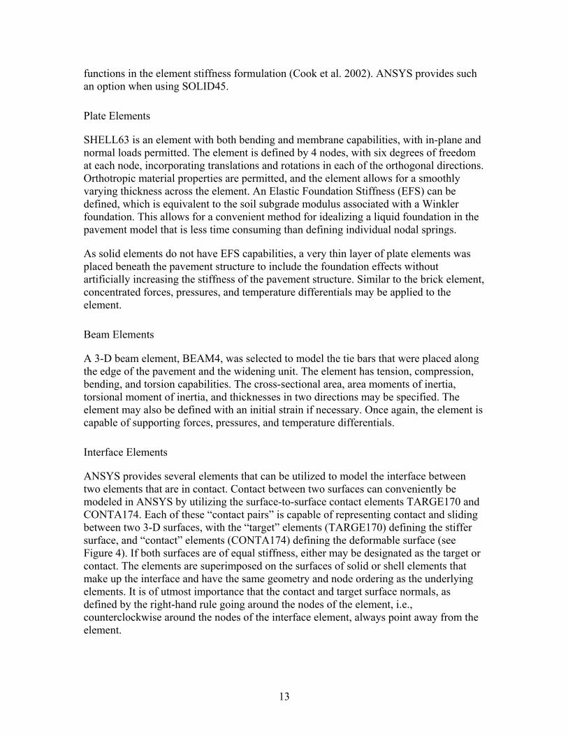
Interface Elements

ANSYS provides several elements that can be utilized to model the interface between two elements that are in contact. Contact between two surfaces can conveniently be modeled in ANSYS by utilizing the surface-to-surface contact elements TARGE170 and CONTA174. Each of these “contact pairs” is capable of representing contact and sliding between two 3-D surfaces, with the “target” elements (TARGE170) defining the stiffer surface, and “contact” elements (CONTA174) defining the deformable surface (see Figure 4). If both surfaces are of equal stiffness, either may be designated as the target or contact. The elements are superimposed on the surfaces of solid or shell elements that make up the interface and have the same geometry and node ordering as the underlying elements. It is of utmost importance that the contact and target surface normals, as defined by the right-hand rule going around the nodes of the element, i.e., counterclockwise around the nodes of the interface element, always point away from the element.

13

Brick Element

Interface Element Surface Normal (Pointing away from Element) (Contact or Target)

Figure 4. Orientation of interface element

The status of contact pairs could either be “closed,” i.e., in contact, or “open,” i.e., not in contact and no load transfer between the two surfaces takes place. Interface elements introduce geometric nonlinearity in the solution process, resulting in increased computing time. Consequently, iterative solutions must be repeated until the status of each interface does not change, while at the same time satisfying the force and displacement convergence criteria and ensuring that penetration between the surfaces stays within acceptable tolerances.

The mechanics of the contact pair involve normal and tangential contact stiffnesses. The normal contact stiffness governs the amount of penetration between the two surfaces. ANSYS estimates the normal contact stiffness based upon the material properties of the underlying elements; however, the stiffness can be adjusted by the user if necessary. Using a larger contact stiffness, while beneficial in reducing penetration, could result in convergence difficulties. Alternatively, a contact stiffness that is too low would allow too much penetration and render the results inaccurate.

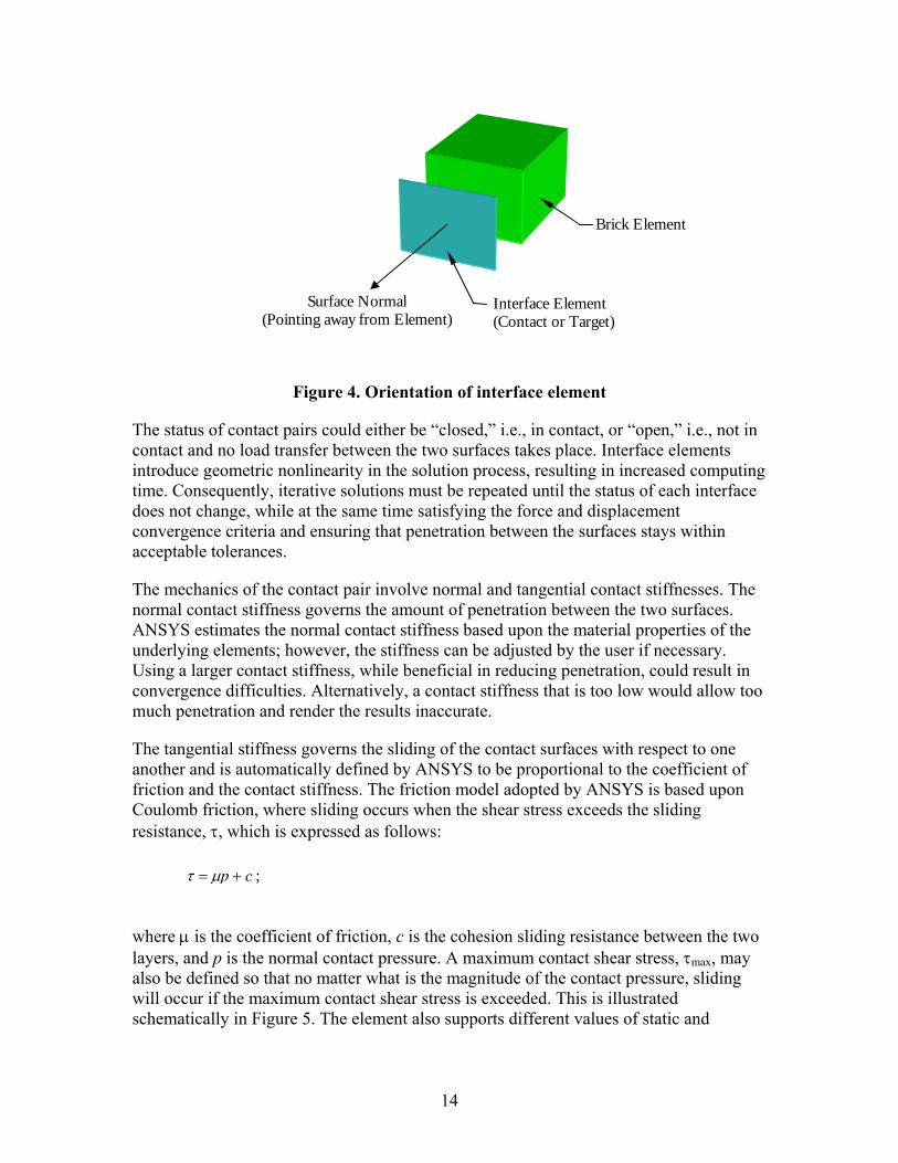
The tangential stiffness governs the sliding of the contact surfaces with respect to one another and is automatically defined by ANSYS to be proportional to the coefficient of friction and the contact stiffness. The friction model adopted by ANSYS is based upon Coulomb friction, where sliding occurs when the shear stress exceeds the sliding resistance, τ, which is expressed as follows:

τ = μp + c ;

where μ is the coefficient of friction, c is the cohesion sliding resistance between the two layers, and p is the normal contact pressure. A maximum contact shear stress, τmax, may also be defined so that no matter what is the magnitude of the contact pressure, sliding will occur if the maximum contact shear stress is exceeded. This is illustrated schematically in Figure 5. The element also supports different values of static and

14

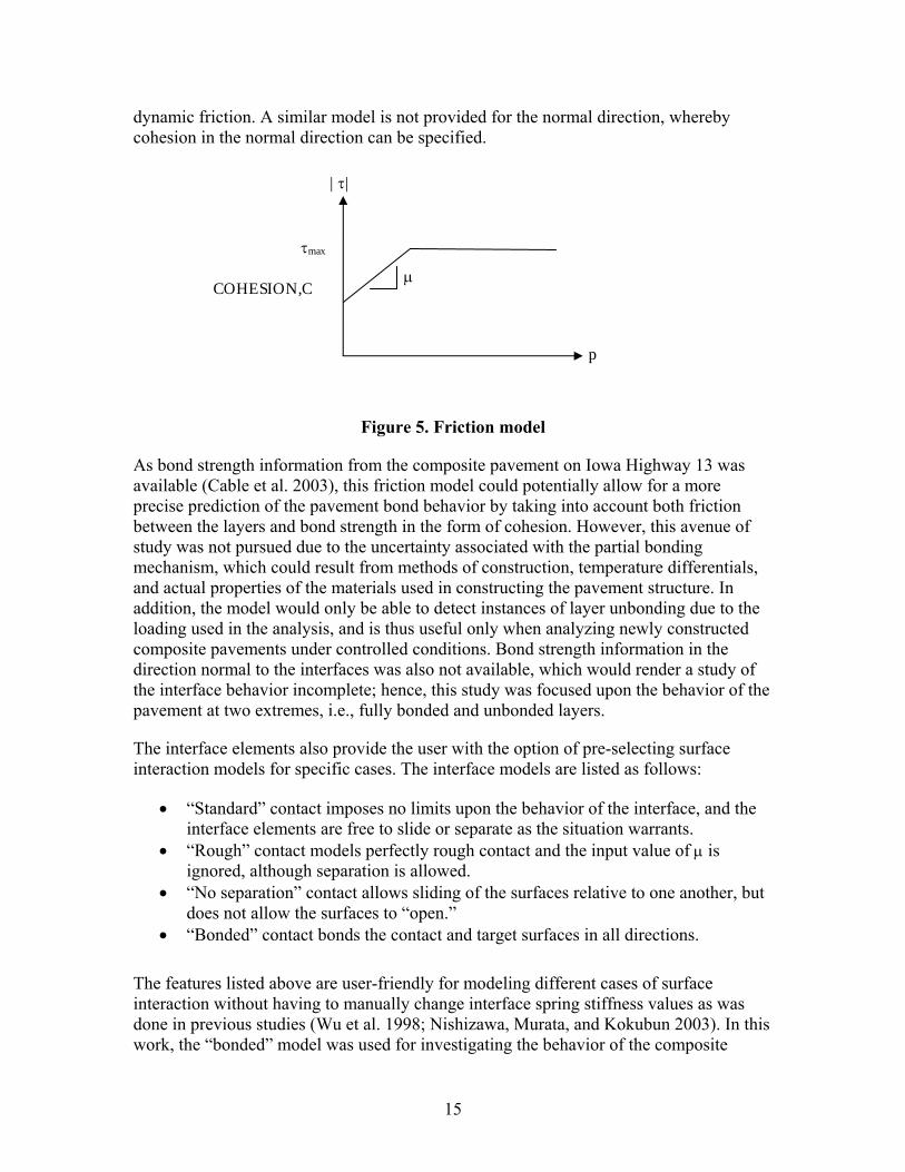
dynamic friction. A similar model is not provided for the normal direction, whereby cohesion in the normal direction can be specified.

|τ|

τmax

COHESION,C

p

μ

Figure 5. Friction model

As bond strength information from the composite pavement on Iowa Highway 13 was available (Cable et al. 2003), this friction model could potentially allow for a more precise prediction of the pavement bond behavior by taking into account both friction between the layers and bond strength in the form of cohesion. However, this avenue of study was not pursued due to the uncertainty associated with the partial bonding mechanism, which could result from methods of construction, temperature differentials, and actual properties of the materials used in constructing the pavement structure. In addition, the model would only be able to detect instances of layer unbonding due to the loading used in the analysis, and is thus useful only when analyzing newly constructed composite pavements under controlled conditions. Bond strength information in the direction normal to the interfaces was also not available, which would render a study of the interface behavior incomplete; hence, this study was focused upon the behavior of the pavement at two extremes, i.e., fully bonded and unbonded layers.

The interface elements also provide the user with the option of pre-selecting surface interaction models for specific cases. The interface models are listed as follows:

• “Standard” contact imposes no limits upon the behavior of the interface, and the interface elements are free to slide or separate as the situation warrants.

• “Rough” contact models perfectly rough contact and the input value of μ is ignored, although separation is allowed.

• “No separation” contact allows sliding of the surfaces relative to one another, but does not allow the surfaces to “open.”

• “Bonded” contact bonds the contact and target surfaces in all directions.

The features listed above are user-friendly for modeling different cases of surface interaction without having to manually change interface spring stiffness values as was done in previous studies (Wu et al. 1998; Nishizawa, Murata, and Kokubun 2003). In this work, the “bonded” model was used for investigating the behavior of the composite

15

pavement when a strong bond exists in all layers. “Standard” or “no separation” was also used for unbonded layers, depending upon whether separation between the surfaces was expected.

Finite Element Modeling of Composite Pavement on Iowa Highway 13

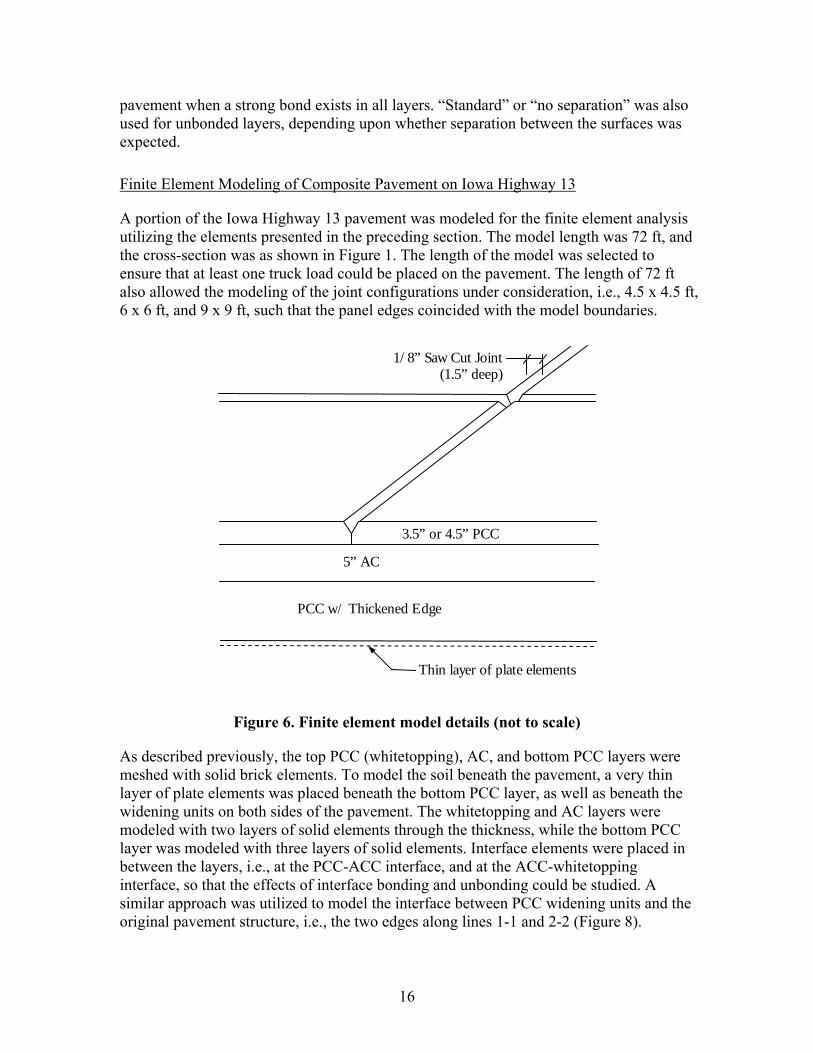
A portion of the Iowa Highway 13 pavement was modeled for the finite element analysis utilizing the elements presented in the preceding section. The model length was 72 ft, and the cross-section was as shown in Figure 1. The length of the model was selected to ensure that at least one truck load could be placed on the pavement. The length of 72 ft also allowed the modeling of the joint configurations under consideration, i.e., 4.5 x 4.5 ft, 6 x 6 ft, and 9 x 9 ft, such that the panel edges coincided with the model boundaries.

1/8” Saw Cut Joint (1.5” deep)

3.5” or 4.5” PCC

5” AC

PCC w/ Thickened Edge

Thin layer of plate elements

Figure 6. Finite element model details (not to scale)

As described previously, the top PCC (whitetopping), AC, and bottom PCC layers were meshed with solid brick elements. To model the soil beneath the pavement, a very thin layer of plate elements was placed beneath the bottom PCC layer, as well as beneath the widening units on both sides of the pavement. The whitetopping and AC layers were modeled with two layers of solid elements through the thickness, while the bottom PCC layer was modeled with three layers of solid elements. Interface elements were placed in between the layers, i.e., at the PCC-ACC interface, and at the ACC-whitetopping interface, so that the effects of interface bonding and unbonding could be studied. A similar approach was utilized to model the interface between PCC widening units and the original pavement structure, i.e., the two edges along lines 1-1 and 2-2 (Figure 8).

16

Saw-cut joints were modeled as V-cuts that were 1/8 in. wide at the whitetopping surface, with a depth of 1.5 in, as shown in Figure 6, per the construction report (Cable et al. 2003). The joint cracks in the model were analyzed with 1.5 in. depth, and with the cracks extending through the thickness of the whitetopping. Apart from the saw-cut joints, the ACC and PCC layers were assumed to be crack-free. Interface elements were utilized between the joints according to the crack depth being studied.

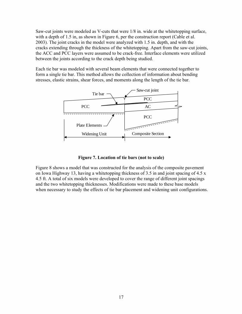
Each tie bar was modeled with several beam elements that were connected together to form a single tie bar. This method allows the collection of information about bending stresses, elastic strains, shear forces, and moments along the length of the tie bar.

PCC

Widening Unit Composite Section

Plate Elements

Tie bar Saw-cut joint

PCC

AC

PCC

Figure 7. Location of tie bars (not to scale)

Figure 8 shows a model that was constructed for the analysis of the composite pavement on Iowa Highway 13, having a whitetopping thickness of 3.5 in and joint spacing of 4.5 x 4.5 ft. A total of six models were developed to cover the range of different joint spacings and the two whitetopping thicknesses. Modifications were made to these base models when necessary to study the effects of tie bar placement and widening unit configurations.

17

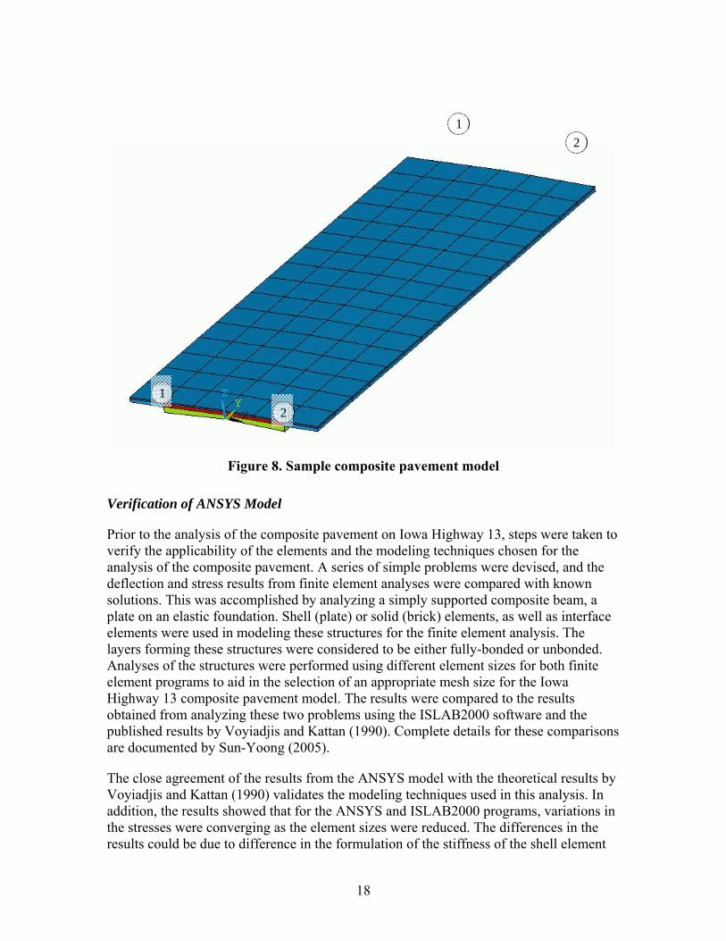
2 1

1 2

Figure 8. Sample composite pavement model

Verification of ANSYS Model

Prior to the analysis of the composite pavement on Iowa Highway 13, steps were taken to verify the applicability of the elements and the modeling techniques chosen for the analysis of the composite pavement. A series of simple problems were devised, and the deflection and stress results from finite element analyses were compared with known solutions. This was accomplished by analyzing a simply supported composite beam, a plate on an elastic foundation. Shell (plate) or solid (brick) elements, as well as interface elements were used in modeling these structures for the finite element analysis. The layers forming these structures were considered to be either fully-bonded or unbonded. Analyses of the structures were performed using different element sizes for both finite element programs to aid in the selection of an appropriate mesh size for the Iowa Highway 13 composite pavement model. The results were compared to the results obtained from analyzing these two problems using the ISLAB2000 software and the published results by Voyiadjis and Kattan (1990). Complete details for these comparisons are documented by Sun-Yoong (2005).

The close agreement of the results from the ANSYS model with the theoretical results by Voyiadjis and Kattan (1990) validates the modeling techniques used in this analysis. In addition, the results showed that for the ANSYS and ISLAB2000 programs, variations in the stresses were converging as the element sizes were reduced. The differences in the results could be due to difference in the formulation of the stiffness of the shell element

18

used in ISLAB2000 and the solid element in ANSYS. These two comparisons also show that the size of the elements to be used in the composite pavement analysis should be limited to a size of 6″ x 6″ or smaller to obtain accurate results. However, one must expect that using smaller size elements will require larger computation time. In this work, element size was limited to 6″ x 6″.

Field Investigation of Iowa Highway 13 Composite Pavement

In order to determine the applicability of utilizing the finite element method to analyze the composite pavement on Iowa Highway 13, field testing of the pavement was carried out. In addition, since soil data was unavailable, it was necessary to determine a representative value suitable for the soil subgrade reaction modulus, ks. This was accomplished by comparing the measured deflection results with analytical results that were obtained using different values for the soil subgrade. Next, the pavement model was analyzed with the selected value of ks to determine the computed strains at the gage locations, which were compared to the measured strains obtained from field testing.

Field Test

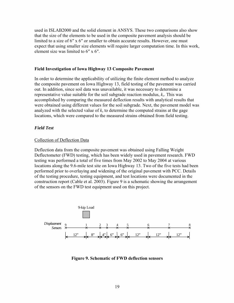
Collection of Deflection Data

Deflection data from the composite pavement was obtained using Falling Weight Deflectometer (FWD) testing, which has been widely used in pavement research. FWD testing was performed a total of five times from May 2002 to May 2004 at various locations along the 9.6-mile test site on Iowa Highway 13. Two of the five tests had been performed prior to overlaying and widening of the original pavement with PCC. Details of the testing procedure, testing equipment, and test locations were documented in the construction report (Cable et al. 2003). Figure 9 is a schematic showing the arrangement of the sensors on the FWD test equipment used on this project.

9-kip Load

Displacement 9 1 2 3 4 5 6 7

12” 8” 4” 6” 6” 12” 12” 12”

Sensors

Figure 9. Schematic of FWD deflection sensors

19

8

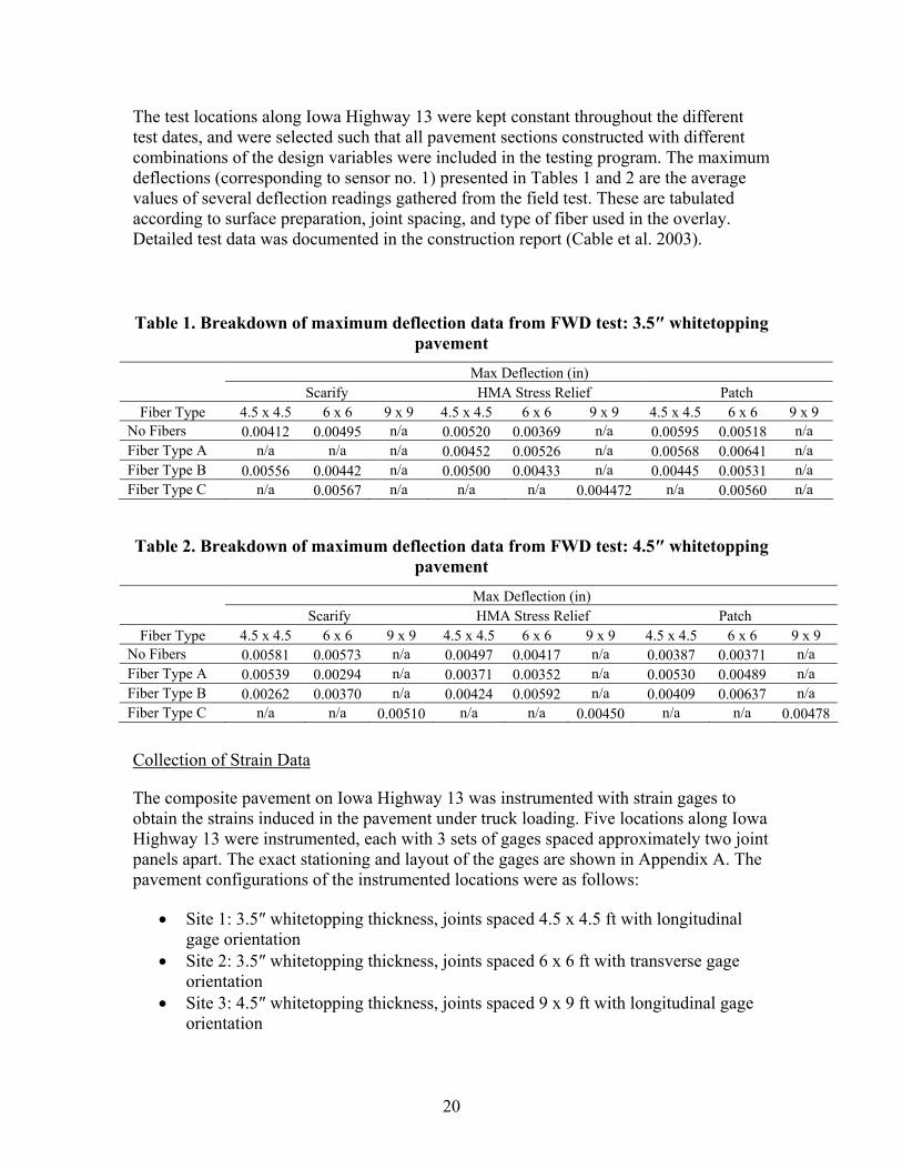
The test locations along Iowa Highway 13 were kept constant throughout the different test dates, and were selected such that all pavement sections constructed with different combinations of the design variables were included in the testing program. The maximum deflections (corresponding to sensor no. 1) presented in Tables 1 and 2 are the average values of several deflection readings gathered from the field test. These are tabulated according to surface preparation, joint spacing, and type of fiber used in the overlay. Detailed test data was documented in the construction report (Cable et al. 2003).

Table 1. Breakdown of maximum deflection data from FWD test: 3.5″ whitetopping pavement

Max Deflection (in) Scarify HMA Stress Relief Patch

Fiber Type 4.5 x 4.5 6 x 6 9 x 9 4.5 x 4.5 6 x 6 9 x 9 4.5 x 4.5 6 x 6 9 x 9 No Fibers 0.00412 0.00495 n/a 0.00520 0.00369 n/a 0.00595 0.00518 n/a Fiber Type A n/a n/a n/a 0.00452 0.00526 n/a 0.00568 0.00641 n/a Fiber Type B 0.00556 0.00442 n/a 0.00500 0.00433 n/a 0.00445 0.00531 n/a Fiber Type C n/a 0.00567 n/a n/a n/a 0.004472 n/a 0.00560 n/a

Table 2. Breakdown of maximum deflection data from FWD test: 4.5″ whitetopping pavement

Max Deflection (in) Scarify HMA Stress Relief Patch

Fiber Type 4.5 x 4.5 6 x 6 9 x 9 4.5 x 4.5 6 x 6 9 x 9 4.5 x 4.5 6 x 6 9 x 9 No Fibers 0.00581 0.00573 n/a 0.00497 0.00417 n/a 0.00387 0.00371 n/a Fiber Type A 0.00539 0.00294 n/a 0.00371 0.00352 n/a 0.00530 0.00489 n/a Fiber Type B 0.00262 0.00370 n/a 0.00424 0.00592 n/a 0.00409 0.00637 n/a Fiber Type C n/a n/a 0.00510 n/a n/a 0.00450 n/a n/a 0.00478

Collection of Strain Data

The composite pavement on Iowa Highway 13 was instrumented with strain gages to obtain the strains induced in the pavement under truck loading. Five locations along Iowa Highway 13 were instrumented, each with 3 sets of gages spaced approximately two joint panels apart. The exact stationing and layout of the gages are shown in Appendix A. The pavement configurations of the instrumented locations were as follows:

• Site 1: 3.5″ whitetopping thickness, joints spaced 4.5 x 4.5 ft with longitudinal gage orientation

• Site 2: 3.5″ whitetopping thickness, joints spaced 6 x 6 ft with transverse gage orientation

• Site 3: 4.5″ whitetopping thickness, joints spaced 9 x 9 ft with longitudinal gage orientation

20

• Site 4: 4.5″ whitetopping thickness, joints spaced 4.5 x 4.5 ft with transverse gage orientation

• Site 5: 4.5″ whitetopping thickness, joints spaced 6 x 6 ft with longitudinal gage orientation

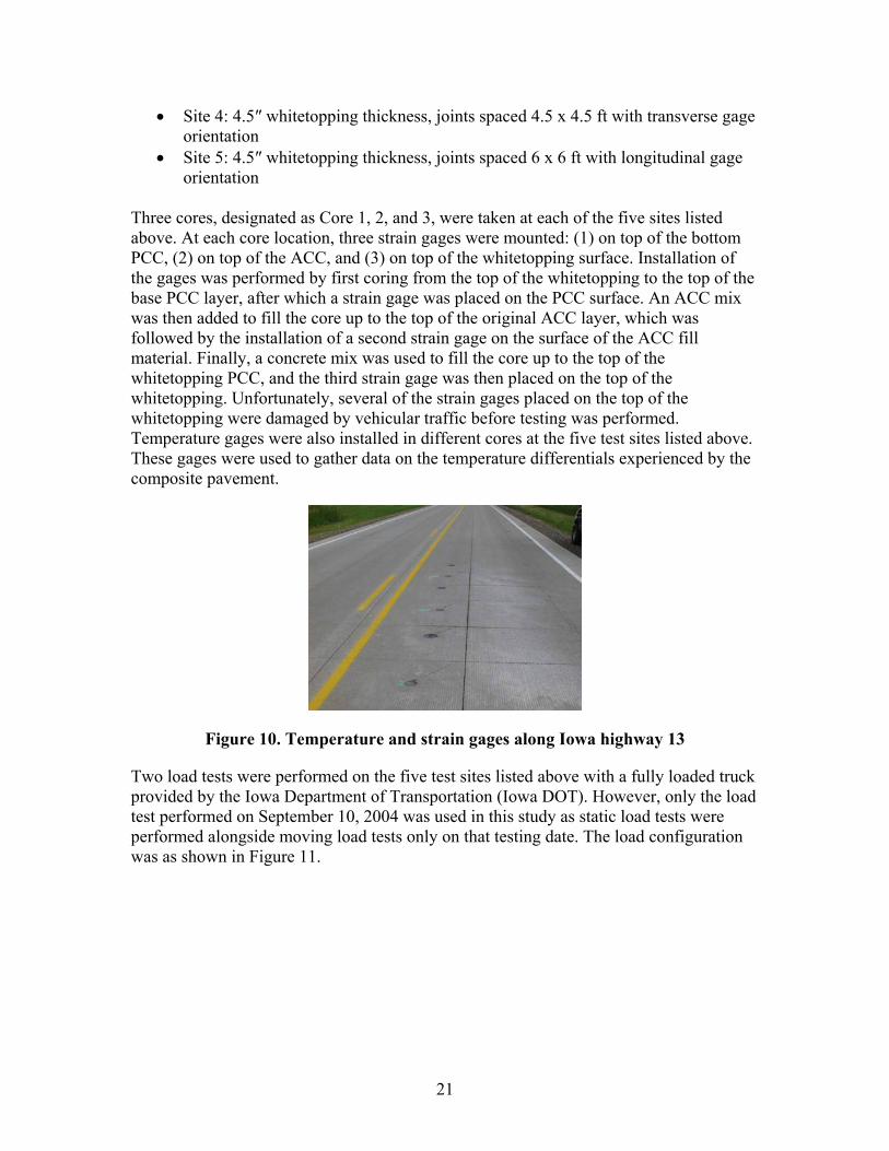
Three cores, designated as Core 1, 2, and 3, were taken at each of the five sites listed above. At each core location, three strain gages were mounted: (1) on top of the bottom PCC, (2) on top of the ACC, and (3) on top of the whitetopping surface. Installation of the gages was performed by first coring from the top of the whitetopping to the top of the base PCC layer, after which a strain gage was placed on the PCC surface. An ACC mix was then added to fill the core up to the top of the original ACC layer, which was followed by the installation of a second strain gage on the surface of the ACC fill material. Finally, a concrete mix was used to fill the core up to the top of the whitetopping PCC, and the third strain gage was then placed on the top of the whitetopping. Unfortunately, several of the strain gages placed on the top of the whitetopping were damaged by vehicular traffic before testing was performed. Temperature gages were also installed in different cores at the five test sites listed above. These gages were used to gather data on the temperature differentials experienced by the composite pavement.

Figure 10. Temperature and strain gages along Iowa highway 13

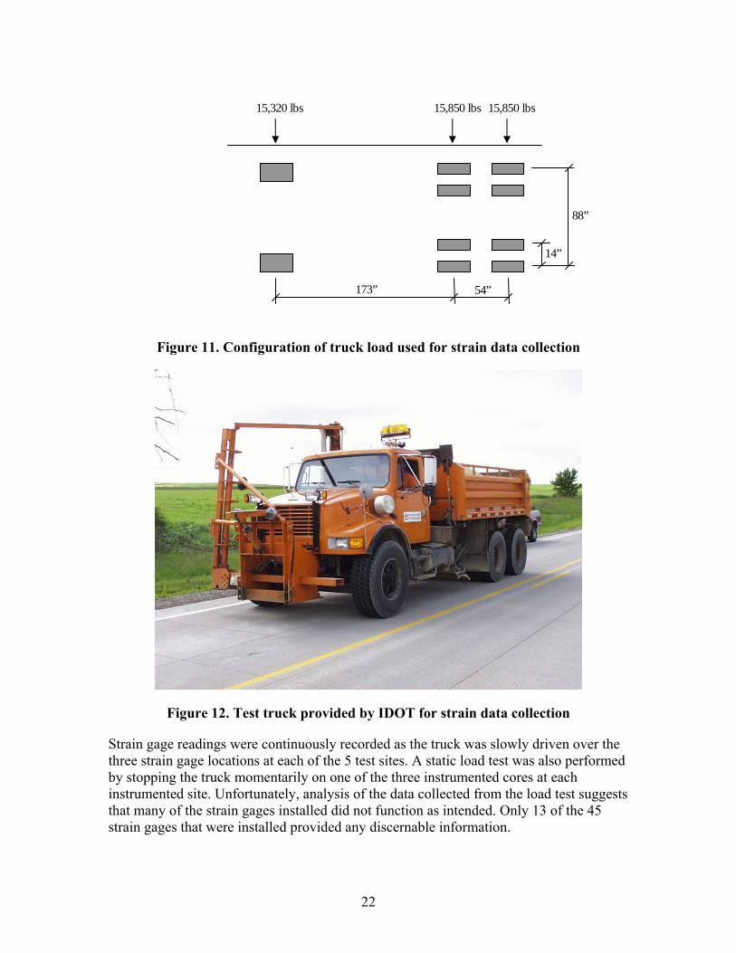
Two load tests were performed on the five test sites listed above with a fully loaded truck provided by the Iowa Department of Transportation (Iowa DOT). However, only the load test performed on September 10, 2004 was used in this study as static load tests were performed alongside moving load tests only on that testing date. The load configuration was as shown in Figure 11.

21

15,320 lbs 15,850 lbs 15,850 lbs

54”

14”

88”

173”

Figure 11. Configuration of truck load used for strain data collection

Figure 12. Test truck provided by IDOT for strain data collection

Strain gage readings were continuously recorded as the truck was slowly driven over the three strain gage locations at each of the 5 test sites. A static load test was also performed by stopping the truck momentarily on one of the three instrumented cores at each instrumented site. Unfortunately, analysis of the data collected from the load test suggests that many of the strain gages installed did not function as intended. Only 13 of the 45 strain gages that were installed provided any discernable information.

22

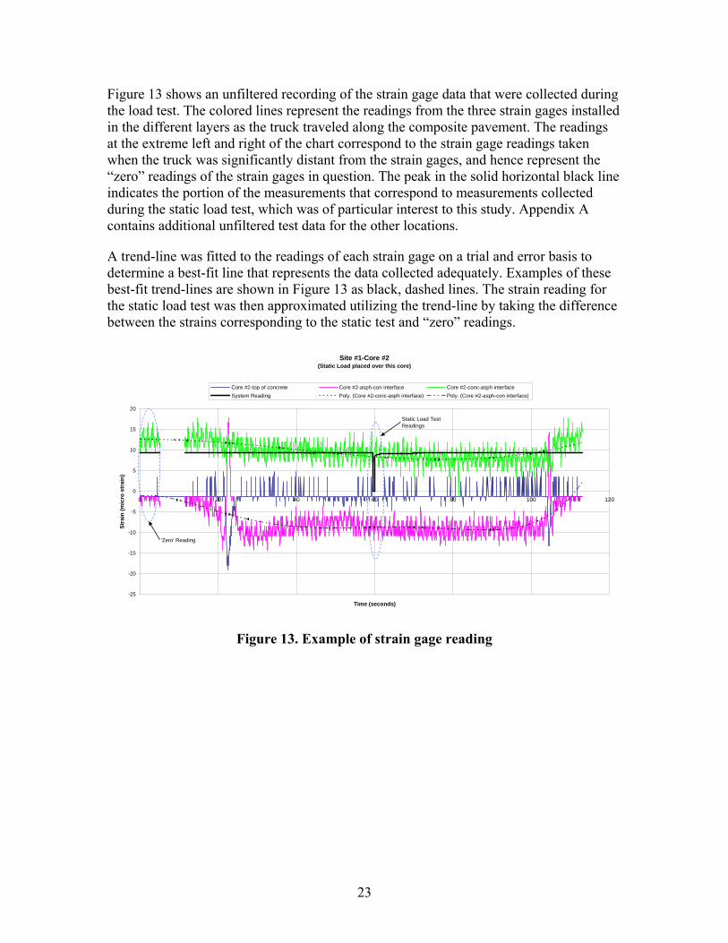
Figure 13 shows an unfiltered recording of the strain gage data that were collected during the load test. The colored lines represent the readings from the three strain gages installed in the different layers as the truck traveled along the composite pavement. The readings at the extreme left and right of the chart correspond to the strain gage readings taken when the truck was significantly distant from the strain gages, and hence represent the “zero” readings of the strain gages in question. The peak in the solid horizontal black line indicates the portion of the measurements that correspond to measurements collected during the static load test, which was of particular interest to this study. Appendix A contains additional unfiltered test data for the other locations.

A trend-line was fitted to the readings of each strain gage on a trial and error basis to determine a best-fit line that represents the data collected adequately. Examples of these best-fit trend-lines are shown in Figure 13 as black, dashed lines. The strain reading for the static load test was then approximated utilizing the trend-line by taking the difference between the strains corresponding to the static test and “zero” readings.

Site #1-Core #2(Static Load placed over this core)

Core #2-top of concrete Core #2-asph-con interface Core #2-conc-asph interface System Reading Poly. (Core #2-conc-asph interface) Poly. (Core #2-asph-con interface)

20

Static Load Test Readings 15

10

5

0 0 20 40 60 80 100 120

-5

-10 'Zero' Reading

-15

-20

-25

Time (seconds)

Figure 13. Example of strain gage reading

Stra

in (m

icro

str

ain)

23

Composite Pavement Analysis with Field Test Loads

The composite pavement on Iowa Highway 13 was analyzed under the different test loads described in the previous section. This required knowledge of the properties of the pavement materials and the soil subgrade reaction. Unfortunately, detailed information regarding these parameters was not available and had to be estimated from well-established norms. Information gathered from communication with Iowa DOT provided an estimate on the compressive strength of the whitetopping layer of 4500psi. The modulus of elasticity for the ACC layer was estimated from common values encountered in the central Iowa region (Coree 2004). Values of the ACC modulus of elasticity from the spring and fall seasons were utilized to reach an estimate of 650,000 psi for the modulus of elasticity of the ACC layer in this study. This value corresponds with the time when the different field tests were performed. Typical values of 0.35 and 0.2 were assumed for the Poisson’s ratio of asphalt and concrete, respectively.

As mentioned previously, information regarding the properties of the soil beneath the pavement was not known; thus, it was necessary to determine the modulus of subgrade reaction, ks, using a different approach. While an estimate of 75 pci was suggested (Cable 2004), the value of ks was estimated based upon the more rational method of comparing analysis results with the deflection data obtained from FWD testing.

Comparison with FWD Deflection Data

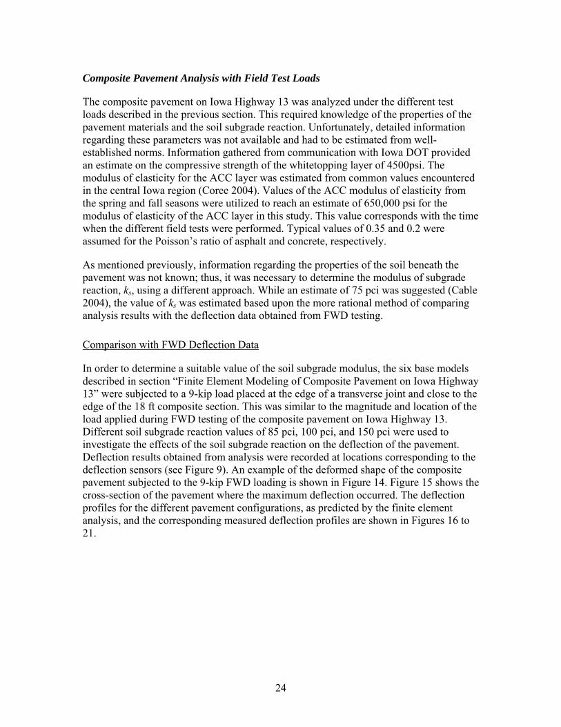
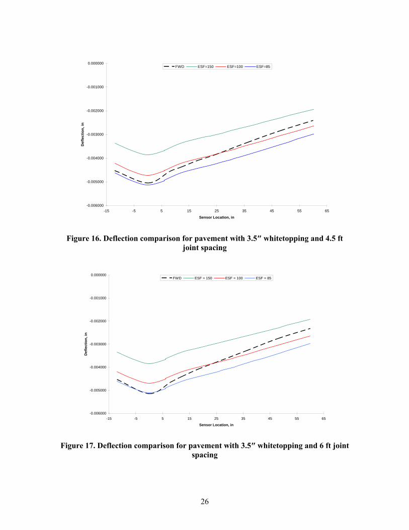
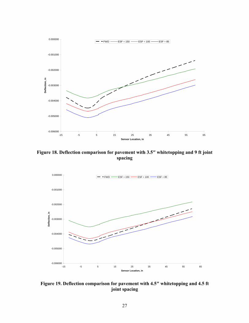
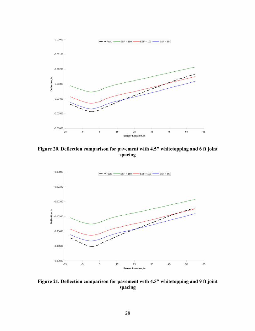
In order to determine a suitable value of the soil subgrade modulus, the six base models described in section “Finite Element Modeling of Composite Pavement on Iowa Highway 13” were subjected to a 9-kip load placed at the edge of a transverse joint and close to the edge of the 18 ft composite section. This was similar to the magnitude and location of the load applied during FWD testing of the composite pavement on Iowa Highway 13. Different soil subgrade reaction values of 85 pci, 100 pci, and 150 pci were used to investigate the effects of the soil subgrade reaction on the deflection of the pavement. Deflection results obtained from analysis were recorded at locations corresponding to the deflection sensors (see Figure 9). An example of the deformed shape of the composite pavement subjected to the 9-kip FWD loading is shown in Figure 14. Figure 15 shows the cross-section of the pavement where the maximum deflection occurred. The deflection profiles for the different pavement configurations, as predicted by the finite element analysis, and the corresponding measured deflection profiles are shown in Figures 16 to 21.

24

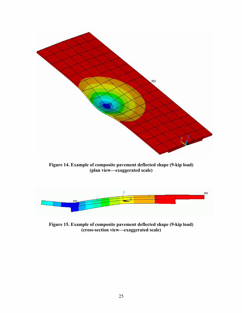
Figure 14. Example of composite pavement deflected shape (9-kip load) (plan view—exaggerated scale)

Figure 15. Example of composite pavement deflected shape (9-kip load) (cross-section view—exaggerated scale)

25

Def

lect

ion,

in

0.000000 FWD ESF=150 ESF=100 ESF=85

-0.001000

-0.002000

-0.003000

-0.004000

-0.005000

-0.006000 -15 -5 5 15 25 35 45 55 65

Sensor Location, in

Figure 16. Deflection comparison for pavement with 3.5″ whitetopping and 4.5 ft joint spacing

Def

lect

ion,

in

0.000000 FWD ESF = 150 ESF = 100 ESF = 85

-0.001000

-0.002000

-0.003000

-0.004000

-0.005000

-0.006000 -15 -5 5 15 25 35 45 55 65

Sensor Location, in

Figure 17. Deflection comparison for pavement with 3.5″ whitetopping and 6 ft joint spacing

26

Def

lect

ion,

in

0.000000 FWD ESF = 150 ESF = 100 ESF = 85

-0.001000

-0.002000

-0.003000

-0.004000

-0.005000

-0.006000 -15 -5 5 15 25

Sensor Location, in 35 45 55 65

Figure 18. Deflection comparison for pavement with 3.5″ whitetopping and 9 ft joint spacing

Def

lect

ion,

in

0.000000 FWD ESF = 150 ESF = 100 ESF = 85

-0.001000

-0.002000

-0.003000

-0.004000

-0.005000

-0.006000 -15 -5 5 15 25 35 45 55 65

Sensor Location, in

Figure 19. Deflection comparison for pavement with 4.5″ whitetopping and 4.5 ft joint spacing

27

Def

lect

ion,

in

0.00000 FWD ESF = 150 ESF = 100 ESF = 85

-0.00100

-0.00200

-0.00300

-0.00400

-0.00500

-0.00600 -15 -5 5 15 25 35 45 55 65

Sensor Location, in

Figure 20. Deflection comparison for pavement with 4.5″ whitetopping and 6 ft joint spacing

Def

lect

ion,

in

0.00000 FWD ESF = 150 ESF = 100 ESF = 85

-0.00100

-0.00200

-0.00300

-0.00400

-0.00500

-0.00600 -15 -5 5 15 25 35 45 55 65

Sensor Location, in

Figure 21. Deflection comparison for pavement with 4.5″ whitetopping and 9 ft joint spacing

28

As can be seen from the preceding figures, the deflections obtained from FWD testing appear to be bounded by ks values of 85~100 pci, and is closer to those obtained using ks of 85 pci. This is slightly different from the estimate of 75 pci (Cable 2004). The lower value of 85 pci was selected as an acceptable value to represent the stiffness of the foundation beneath the composite pavement on Iowa Highway 13 and was utilized in all subsequent finite element analyses in this study.

Comparison with Measured Strain Data

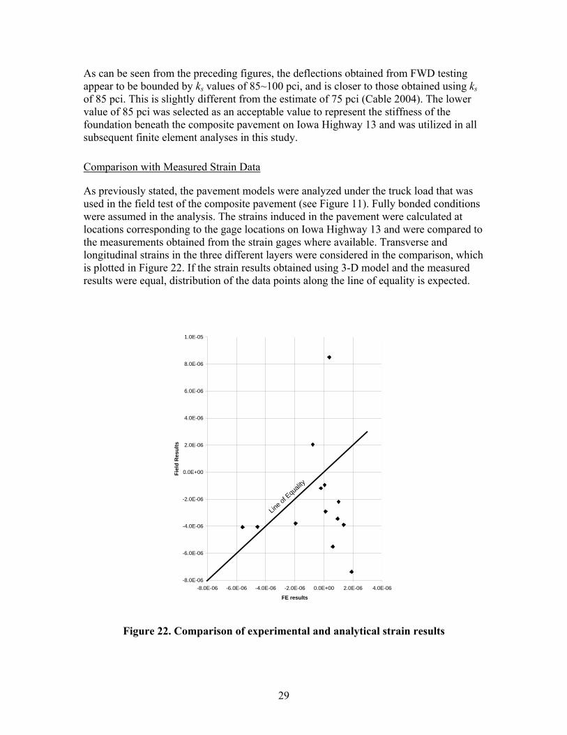
As previously stated, the pavement models were analyzed under the truck load that was used in the field test of the composite pavement (see Figure 11). Fully bonded conditions were assumed in the analysis. The strains induced in the pavement were calculated at locations corresponding to the gage locations on Iowa Highway 13 and were compared to the measurements obtained from the strain gages where available. Transverse and longitudinal strains in the three different layers were considered in the comparison, which is plotted in Figure 22. If the strain results obtained using 3-D model and the measured results were equal, distribution of the data points along the line of equality is expected.

Fiel

d R

esul

ts

1.0E-05

8.0E-06

6.0E-06

4.0E-06

2.0E-06

0.0E+00

-2.0E-06

-4.0E-06

-6.0E-06

-8.0E-06

Line of

Equalit

y

-8.0E-06 -6.0E-06 -4.0E-06 -2.0E-06 0.0E+00 2.0E-06 4.0E-06

FE results

Figure 22. Comparison of experimental and analytical strain results

29

The above comparison shows some discrepancy between the results from the finite element analysis and field test results. However, the strains obtained from finite element analysis and from the field test data were both in the range of -10 to 10 microns, while the error of the strain gages used was in the range of 4~5 microns. This could be a significant part of the reason for the poor agreement between experimental and analytical results. In addition, the method of installation of the strain gages could also have contributed to the discrepancy, as removal of the original pavement material could have altered the behavior of the pavement at the strain gage locations, which can not be accurately accounted for in the 3-D model. As most of the strain gages that were installed had malfunctioned or were damaged, the accuracy of the data from the remaining strain gages that was deemed useful could also be suspect. Interference from passing traffic while the truck load testing was performed could also have easily contributed to further error in the experimental results.

Not all reasons for the discrepancy were due to experimental factors. Localized differences in the soil properties from test site to test site could exist and would require that different values for the soil subgrade reaction be used instead of the 85 pci determined previously. Simplification of the model by assuming perfectly undamaged ACC and PCC layers underlying the whitetopping could be another source of error. Additionally, the degree of bond at the interfaces between the layers is potentially another factor contributing to the discrepancy between experimental and analytical results. Unfortunately, a lack of information regarding actual field conditions and interaction mechanism renders a highly detailed model which adequately accounts for all these factors improbable in the current analysis.

With the many factors potentially contributing to the discrepancy between field data and analytical strain values, the comparison is thus inconclusive and no determination can be made regarding the accuracy of the finite element model based upon these strain results alone. However, the favorable comparison between the deflection values and deflection profiles recorded from the field, and those obtained from analyses, generated sufficient confidence in the results from the finite element model. Hence, the finite element model was further utilized to investigate the behavior of the composite pavement on Iowa Highway 13.

30

Analysis of Iowa Highway 13 Composite Pavement

Following the verification of the pavement model developed for the finite element program ANSYS, the 3-D composite pavement model was subjected to different loading conditions. A parametric study was carried out to investigate the effects that whitetopping thickness, interface bonding, joint spacing, depth of joint crack, widening unit configuration, and tie bar size and spacing have on overall structural behavior. The pavement was then subjected to heavy truckloads, and temperature gradients were recorded from the installed gages to determine the stresses that could be induced in the composite pavement in the field.

Parametric Study of Composite Pavement

Of particular interest in the study presented herein are the effects of the following factors on pavement behavior:

• Thickness of the whitetopping • Spacing of the joints • Depth of the cracks along the joints • Bonding of the layers • Width and depth of the widening units • Size and spacing of tie bars

Therefore, the composite pavement was analyzed considering each of the variables listed above. As mentioned in chapter “Modeling of Iowa Highway 13 Composite Pavement,” in the development of the 3-D finite element model, only the saw-cut joints in the whitetopping layer were modeled, and the rest of the pavement structure was assumed to be un-cracked. The soil subgrade reaction modulus, ks, was assumed to be 85 pci. The pavement layers were considered to be fully bonded to one another, except when investigating the effects of interface bond behavior. Material properties of the different layers listed in the previous chapter were again utilized in this portion of the study. For the purposes of the parametric study, the pavement was subjected to a 9-kip load located at the edge of a transverse saw-cut joint and at the edge of the widening unit–composite section longitudinal joint shown in Figure 7.

Whitetopping Thickness and Joint Spacing

The whitetopping overlay on Iowa Highway 13 was constructed with two different thicknesses. One should expect that the thicker whitetopping would provide better pavement performance. In order to quantify this difference in the behavior of the composite pavement, a total of six pavement models, configured with combinations of the two whitetopping thicknesses (3.5 in. and 4.5 in.) and three saw-cut joint configurations (4.5 x 4.5 ft, 6 x 6 ft and 9 x 9 ft), were analyzed under a 9-kip load. Deflection profiles, similar to those obtained by FWD testing, were constructed from the results of the analyses and are presented in Figure 23. The numerical values for the maximum deflection for each case are tabulated in Table 3. The maximum compressive

31

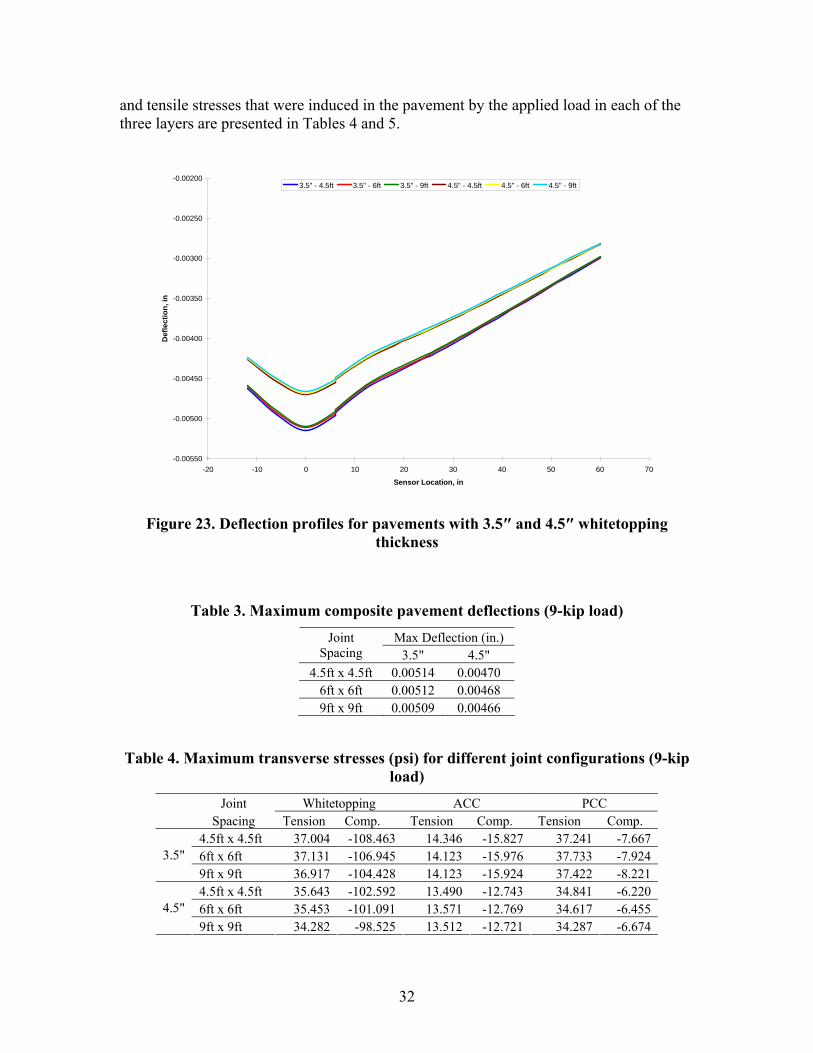
and tensile stresses that were induced in the pavement by the applied load in each of the three layers are presented in Tables 4 and 5.

Def

lect

ion,

in

-0.00200 3.5" - 4.5ft 3.5" - 6ft 3.5" - 9ft 4.5" - 4.5ft 4.5" - 6ft 4.5" - 9ft

-0.00250

-0.00300

-0.00350

-0.00400

-0.00450

-0.00500

-0.00550 -20 -10 0 10 20 30 40 50 60 70

Sensor Location, in

Figure 23. Deflection profiles for pavements with 3.5″ and 4.5″ whitetopping thickness

Table 3. Maximum composite pavement deflections (9-kip load) Joint Max Deflection (in.)

Spacing 3.5" 4.5" 4.5ft x 4.5ft 0.00514 0.00470

6ft x 6ft 0.00512 0.00468 9ft x 9ft 0.00509 0.00466

Table 4. Maximum transverse stresses (psi) for different joint configurations (9-kip load)

Joint Whitetopping ACC PCC Spacing Tension Comp. Tension Comp. Tension Comp.

4.5ft x 4.5ft 37.004 -108.463 14.346 -15.827 37.241 -7.667 3.5" 6ft x 6ft 37.131 -106.945 14.123 -15.976 37.733 -7.924

9ft x 9ft 36.917 -104.428 14.123 -15.924 37.422 -8.221 4.5ft x 4.5ft 35.643 -102.592 13.490 -12.743 34.841 -6.220

4.5" 6ft x 6ft 35.453 -101.091 13.571 -12.769 34.617 -6.455 9ft x 9ft 34.282 -98.525 13.512 -12.721 34.287 -6.674

32

Table 5. Maximum longitudinal stresses (psi) for different joint configurations (9-kip load)

Joint Whitetopping ACC PCC Spacing Tension Comp. Tension Comp. Tension Comp.

4.5ft x 4.5ft 31.729 -123.174 11.544 -17.347 70.942 -16.835 3.5" 6ft x 6ft 31.079 -122.264 11.428 -17.514 70.560 -16.633

9ft x 9ft 30.530 -121.010 11.415 -17.435 70.162 -16.572 4.5ft x 4.5ft 31.528 -113.645 10.832 -13.994 62.897 -11.745

4.5" 6ft x 6ft 31.000 -112.791 10.899 -14.036 62.615 -11.744 9ft x 9ft 30.466 -111.497 10.863 -13.960 62.309 -11.690

As can be seen from Figure 23 and Table 3, the deflections experienced by the pavements with thinner whitetopping overlays were about 10% larger than those with 4.5″ overlays. The pavements with thicker whitetopping overlays also exhibited lower stresses, particularly in the longitudinal direction, in the range of 5.5% to 7.9% for stresses in the whitetopping layer. The thicker whitetopping layer also reduced stresses in the underlying ACC and PCC layers, with reduction of up to 11.2% in the tensile stresses at the bottom PCC layer. The combination of deflection and stress results indicate that the 4.5″ overlay exhibits better performance with deflections and stresses as the design criteria.

The deflection profiles in Figure 23 also seem to suggest that the different joint spacings do not significantly affect pavement behavior when subjected to vertical loads. While overlays with joint spacing at 4.5 x 4.5 ft had the largest deflection and stresses, and overlays of 9 x 9 ft joint spacing exhibited the least amount of deflection and stresses for both thicknesses, the differences were not significant. This contradicts findings from other studies (Tarr, Sheehan, and Okamoto 1998; Kumara et al. 2003), which demonstrate that pavement deflection varies with joint spacing, especially when subjected to temperature loading. The reason for the discrepancy with the findings of other studies was due to the assumption made in the current study that the underlying ACC and PCC layers were crack-free and continuous, while other studies focused on the testing or analyzing of composite pavement panels in isolation. This demonstrates that the condition of the layers underlying the overlay has a significant effect on pavement behavior.

Joint Crack Depth

The saw-cut joints in the whitetopping were modeled with two different depths to determine the effects of joint crack propagation through the depth of the overlay on pavement behavior. Pavement models with 3.5″ whitetopping overlay and the three different joint spacings were analyzed considering the two different crack depths, and the maximum deflections obtained are tabulated in Table 6.

33

Table 6. Maximum deflections due to varying overlay crack depths (9-kip load) Joint Max. Deflections (in)

Spacing 1.5" Full Depth 4.5ft x 4.5ft 0.00514 0.00526 6ft x 6ft 0.00512 0.00522 9ft x 9ft 0.00509 0.00516

The results in Table 6 revealed that modeling the joints assuming that the cracks propagated through the depth of the overlay only resulted in slightly larger deflections. The deflection profiles for the models with full overlay depth cracks exhibited the same behavior as the corresponding model with 1.5″ crack depth. The maximum stresses in the pavement layers with the joints modeled as cracked through the overlay thickness are given in Table 7.

Table 7. Maximum stresses (psi) for full overlay depth joint cracks (9-kip load)

Joint Spacing WhitetoppingTension Comp.

ACC Tension Comp.

PCC Tension Comp.

Transverse: 4.5ft x 4.5ft 38.747 -107.409 14.880 -16.096 39.331 -8.566 6ft x 6ft 38.226 -105.969 14.775 -16.03 38.803 -7.973 9ft x 9ft 37.795 -102.956 14.645 -16.088 38.371 -8.542 Longitudinal: 4.5ft x 4.5ft 31.998 -113.212 11.646 -17.837 72.920 -17.535 6ft x 6ft 31.381 -114.030 11.578 -17.721 72.175 -17.342 9ft x 9ft 30.692 -110.502 11.508 -17.716 71.429 -17.211

The results from Table 7 were compared to the transverse and longitudinal stresses for 3.5″ whitetopping presented in Tables 4 and 5. While the stresses induced in models with joints modeled as full overlay depth cracks were generally larger, the differences between the cases were not significant. The small differences in deflection and stresses obtained from analysis could once again be attributed to the assumption of undamaged and crack-free ACC and PCC layers underlying the whitetopping overlay.

Bond Condition Between Layers

The effect of the interface bond on pavement behavior was investigated by analyzing the composite behavior by assuming either full bonding between all three layers or no bonding between all three layers, thus providing results for two extreme cases. The whitetopping overlay thickness was assumed to be 3.5 in. for this comparison, and the three different joint configurations of 4.5 x 4.5 ft, 6 x 6 ft, and 9 x 9 ft were also included in the investigation. Figure 24 compares the deflection profiles obtained from the analyses and demonstrates that interface bonding significantly affects the deflection behavior of the pavement.

34

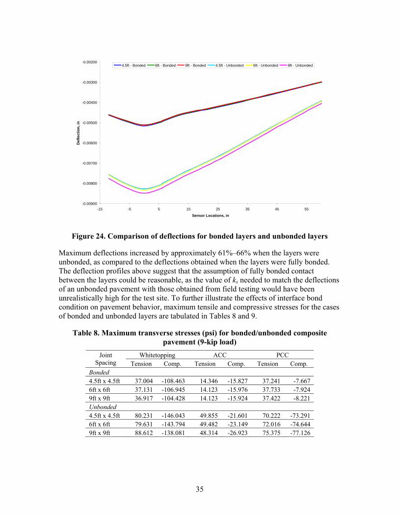
Def

lect

ion,

in

-0.00200 4.5ft - Bonded 6ft - Bonded 9ft - Bonded 4.5ft - Unbonded 6ft - Unbonded 9ft - Unbonded

-0.00300

-0.00400

-0.00500

-0.00600

-0.00700

-0.00800

-0.00900 -15 -5 5 15 25 35 45 55

Sensor Locations, in

Figure 24. Comparison of deflections for bonded layers and unbonded layers

Maximum deflections increased by approximately 61%–66% when the layers were unbonded, as compared to the deflections obtained when the layers were fully bonded. The deflection profiles above suggest that the assumption of fully bonded contact between the layers could be reasonable, as the value of ks needed to match the deflections of an unbonded pavement with those obtained from field testing would have been unrealistically high for the test site. To further illustrate the effects of interface bond condition on pavement behavior, maximum tensile and compressive stresses for the cases of bonded and unbonded layers are tabulated in Tables 8 and 9.

Table 8. Maximum transverse stresses (psi) for bonded/unbonded composite pavement (9-kip load)

Joint Whitetopping ACC PCC Spacing Tension Comp. Tension Comp. Tension Comp.

Bonded 4.5ft x 4.5ft 37.004 -108.463 14.346 -15.827 37.241 -7.667 6ft x 6ft 37.131 -106.945 14.123 -15.976 37.733 -7.924 9ft x 9ft 36.917 -104.428 14.123 -15.924 37.422 -8.221 Unbonded 4.5ft x 4.5ft 80.231 -146.043 49.855 -21.601 70.222 -73.291 6ft x 6ft 79.631 -143.794 49.482 -23.149 72.016 -74.644 9ft x 9ft 88.612 -138.081 48.314 -26.923 75.375 -77.126

35

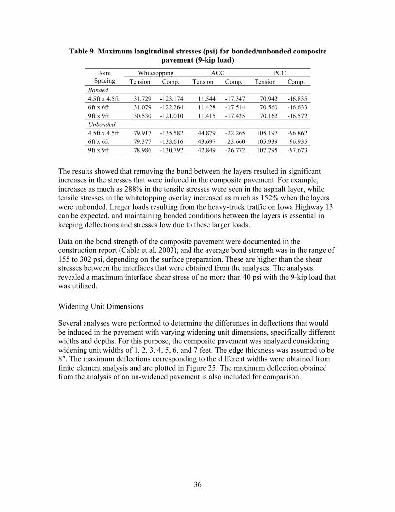
Table 9. Maximum longitudinal stresses (psi) for bonded/unbonded composite pavement (9-kip load)

Joint Whitetopping ACC PCC Spacing Tension Comp. Tension Comp. Tension Comp.

Bonded 4.5ft x 4.5ft 31.729 -123.174 11.544 -17.347 70.942 -16.835 6ft x 6ft 31.079 -122.264 11.428 -17.514 70.560 -16.633 9ft x 9ft 30.530 -121.010 11.415 -17.435 70.162 -16.572 Unbonded 4.5ft x 4.5ft 79.917 -135.582 44.879 -22.265 105.197 -96.862 6ft x 6ft 79.377 -133.616 43.697 -23.660 105.939 -96.935 9ft x 9ft 78.986 -130.792 42.849 -26.772 107.795 -97.673

The results showed that removing the bond between the layers resulted in significant increases in the stresses that were induced in the composite pavement. For example, increases as much as 288% in the tensile stresses were seen in the asphalt layer, while tensile stresses in the whitetopping overlay increased as much as 152% when the layers were unbonded. Larger loads resulting from the heavy-truck traffic on Iowa Highway 13 can be expected, and maintaining bonded conditions between the layers is essential in keeping deflections and stresses low due to these larger loads.

Data on the bond strength of the composite pavement were documented in the construction report (Cable et al. 2003), and the average bond strength was in the range of 155 to 302 psi, depending on the surface preparation. These are higher than the shear stresses between the interfaces that were obtained from the analyses. The analyses revealed a maximum interface shear stress of no more than 40 psi with the 9-kip load that was utilized.

Widening Unit Dimensions

Several analyses were performed to determine the differences in deflections that would be induced in the pavement with varying widening unit dimensions, specifically different widths and depths. For this purpose, the composite pavement was analyzed considering widening unit widths of 1, 2, 3, 4, 5, 6, and 7 feet. The edge thickness was assumed to be 8″. The maximum deflections corresponding to the different widths were obtained from finite element analysis and are plotted in Figure 25. The maximum deflection obtained from the analysis of an un-widened pavement is also included for comparison.

36

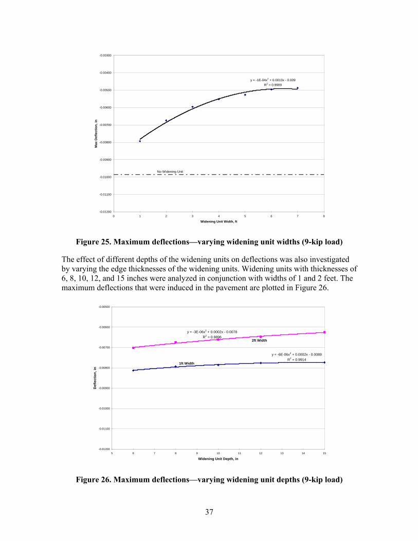
-0.00300

-0.00400

y = -1E-04x2 + 0.0013x - 0.009 R2 = 0.9909

-0.00500

Max

Def

lect

ion,

in

-0.00600

-0.00700

-0.00800

-0.00900

No Widening Unit -0.01000

-0.01100

-0.01200 0 1 2 3 4 5 6 7 8

Widening Unit Width, ft

Figure 25. Maximum deflections—varying widening unit widths (9-kip load)

The effect of different depths of the widening units on deflections was also investigated by varying the edge thicknesses of the widening units. Widening units with thicknesses of 6, 8, 10, 12, and 15 inches were analyzed in conjunction with widths of 1 and 2 feet. The maximum deflections that were induced in the pavement are plotted in Figure 26.

-0.00500

-0.00600

y = -3E-06x2 + 0.0002x - 0.0078 R2 = 0.9896

2ft Width

-0.00700

y = -6E-06x2 + 0.0002x - 0.0089 R2 = 0.9914

1ft Width

Def

lect

ion,

in -0.00800

-0.00900

-0.01000

-0.01100

-0.01200 5 6 7 8 9 10 11 12 13 14 15

Widening Unit Depth, in

Figure 26. Maximum deflections—varying widening unit depths (9-kip load)

37

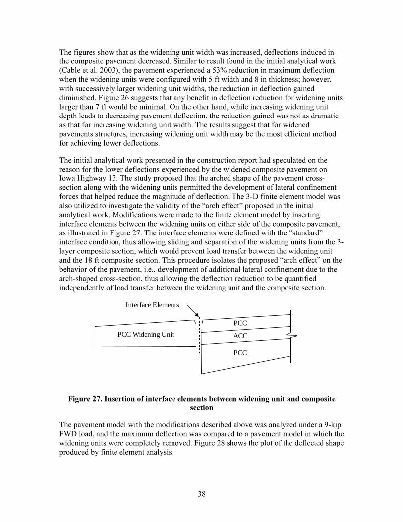
The figures show that as the widening unit width was increased, deflections induced in the composite pavement decreased. Similar to result found in the initial analytical work (Cable et al. 2003), the pavement experienced a 53% reduction in maximum deflection when the widening units were configured with 5 ft width and 8 in thickness; however, with successively larger widening unit widths, the reduction in deflection gained diminished. Figure 26 suggests that any benefit in deflection reduction for widening units larger than 7 ft would be minimal. On the other hand, while increasing widening unit depth leads to decreasing pavement deflection, the reduction gained was not as dramatic as that for increasing widening unit width. The results suggest that for widened pavements structures, increasing widening unit width may be the most efficient method for achieving lower deflections.

The initial analytical work presented in the construction report had speculated on the reason for the lower deflections experienced by the widened composite pavement on Iowa Highway 13. The study proposed that the arched shape of the pavement cross-section along with the widening units permitted the development of lateral confinement forces that helped reduce the magnitude of deflection. The 3-D finite element model was also utilized to investigate the validity of the “arch effect” proposed in the initial analytical work. Modifications were made to the finite element model by inserting interface elements between the widening units on either side of the composite pavement, as illustrated in Figure 27. The interface elements were defined with the “standard” interface condition, thus allowing sliding and separation of the widening units from the 3­layer composite section, which would prevent load transfer between the widening unit and the 18 ft composite section. This procedure isolates the proposed “arch effect” on the behavior of the pavement, i.e., development of additional lateral confinement due to the arch-shaped cross-section, thus allowing the deflection reduction to be quantified independently of load transfer between the widening unit and the composite section.

Interface Elements

PCC Widening Unit

PCC

ACC

PCC

Figure 27. Insertion of interface elements between widening unit and composite section

The pavement model with the modifications described above was analyzed under a 9-kip FWD load, and the maximum deflection was compared to a pavement model in which the widening units were completely removed. Figure 28 shows the plot of the deflected shape produced by finite element analysis.

38

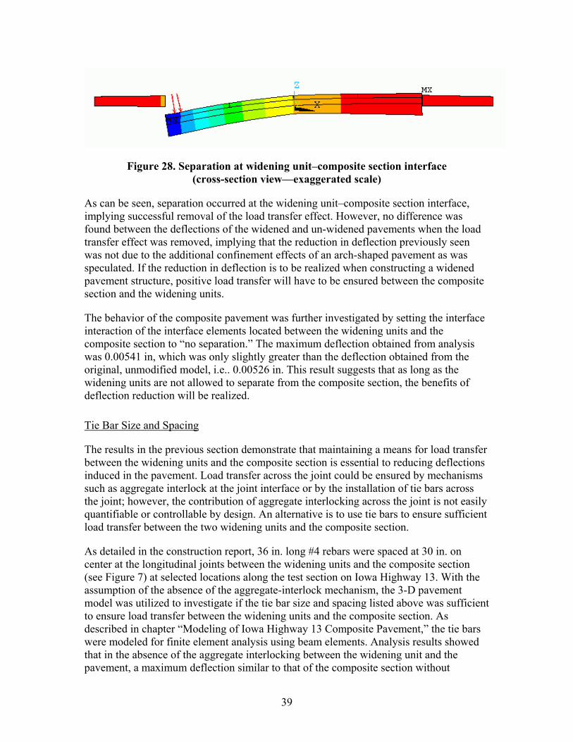
Figure 28. Separation at widening unit–composite section interface (cross-section view—exaggerated scale)

As can be seen, separation occurred at the widening unit–composite section interface, implying successful removal of the load transfer effect. However, no difference was found between the deflections of the widened and un-widened pavements when the load transfer effect was removed, implying that the reduction in deflection previously seen was not due to the additional confinement effects of an arch-shaped pavement as was speculated. If the reduction in deflection is to be realized when constructing a widened pavement structure, positive load transfer will have to be ensured between the composite section and the widening units.

The behavior of the composite pavement was further investigated by setting the interface interaction of the interface elements located between the widening units and the composite section to “no separation.” The maximum deflection obtained from analysis was 0.00541 in, which was only slightly greater than the deflection obtained from the original, unmodified model, i.e.. 0.00526 in. This result suggests that as long as the widening units are not allowed to separate from the composite section, the benefits of deflection reduction will be realized.

Tie Bar Size and Spacing

The results in the previous section demonstrate that maintaining a means for load transfer between the widening units and the composite section is essential to reducing deflections induced in the pavement. Load transfer across the joint could be ensured by mechanisms such as aggregate interlock at the joint interface or by the installation of tie bars across the joint; however, the contribution of aggregate interlocking across the joint is not easily quantifiable or controllable by design. An alternative is to use tie bars to ensure sufficient load transfer between the two widening units and the composite section.

As detailed in the construction report, 36 in. long #4 rebars were spaced at 30 in. on center at the longitudinal joints between the widening units and the composite section (see Figure 7) at selected locations along the test section on Iowa Highway 13. With the assumption of the absence of the aggregate-interlock mechanism, the 3-D pavement model was utilized to investigate if the tie bar size and spacing listed above was sufficient to ensure load transfer between the widening units and the composite section. As described in chapter “Modeling of Iowa Highway 13 Composite Pavement,” the tie bars were modeled for finite element analysis using beam elements. Analysis results showed that in the absence of the aggregate interlocking between the widening unit and the pavement, a maximum deflection similar to that of the composite section without

39

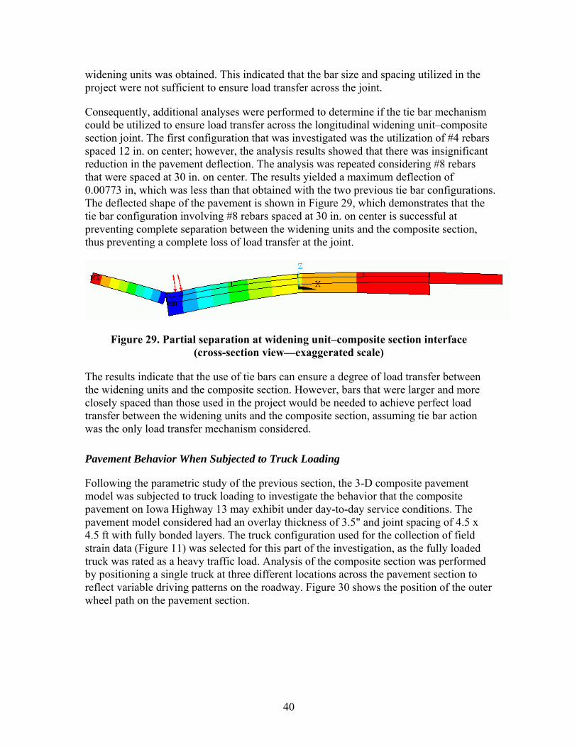
widening units was obtained. This indicated that the bar size and spacing utilized in the project were not sufficient to ensure load transfer across the joint.

Consequently, additional analyses were performed to determine if the tie bar mechanism could be utilized to ensure load transfer across the longitudinal widening unit–composite section joint. The first configuration that was investigated was the utilization of #4 rebars spaced 12 in. on center; however, the analysis results showed that there was insignificant reduction in the pavement deflection. The analysis was repeated considering #8 rebars that were spaced at 30 in. on center. The results yielded a maximum deflection of 0.00773 in, which was less than that obtained with the two previous tie bar configurations. The deflected shape of the pavement is shown in Figure 29, which demonstrates that the tie bar configuration involving #8 rebars spaced at 30 in. on center is successful at preventing complete separation between the widening units and the composite section, thus preventing a complete loss of load transfer at the joint.

Figure 29. Partial separation at widening unit–composite section interface (cross-section view—exaggerated scale)

The results indicate that the use of tie bars can ensure a degree of load transfer between the widening units and the composite section. However, bars that were larger and more closely spaced than those used in the project would be needed to achieve perfect load transfer between the widening units and the composite section, assuming tie bar action was the only load transfer mechanism considered.

Pavement Behavior When Subjected to Truck Loading

Following the parametric study of the previous section, the 3-D composite pavement model was subjected to truck loading to investigate the behavior that the composite pavement on Iowa Highway 13 may exhibit under day-to-day service conditions. The pavement model considered had an overlay thickness of 3.5" and joint spacing of 4.5 x 4.5 ft with fully bonded layers. The truck configuration used for the collection of field strain data (Figure 11) was selected for this part of the investigation, as the fully loaded truck was rated as a heavy traffic load. Analysis of the composite section was performed by positioning a single truck at three different locations across the pavement section to reflect variable driving patterns on the roadway. Figure 30 shows the position of the outer wheel path on the pavement section.

40

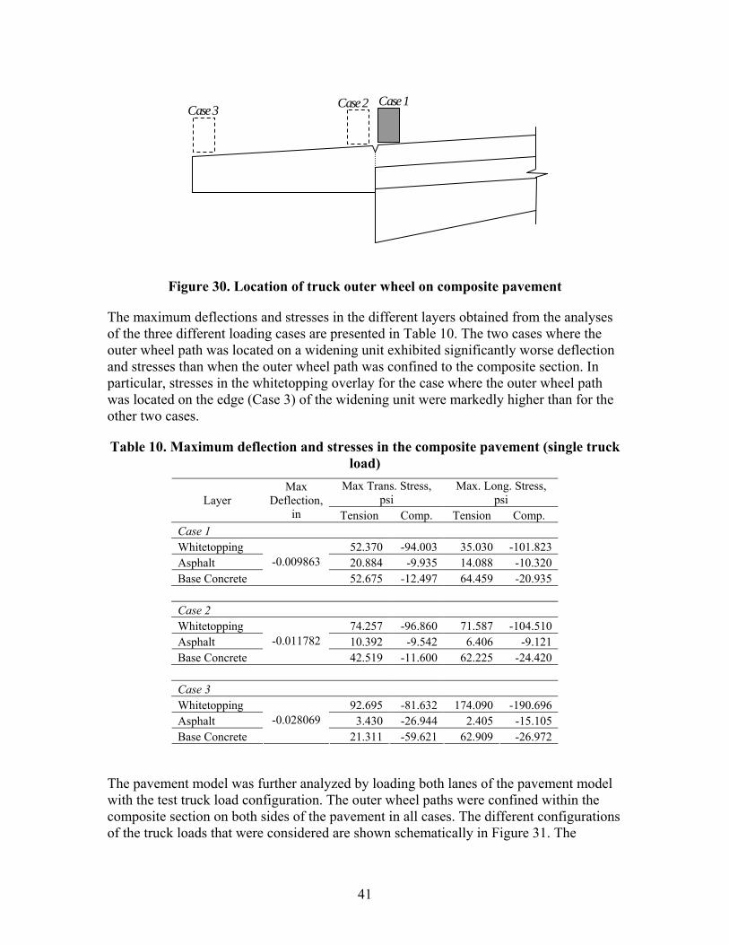
Case 2 Case 1 Case 3

Figure 30. Location of truck outer wheel on composite pavement

The maximum deflections and stresses in the different layers obtained from the analyses of the three different loading cases are presented in Table 10. The two cases where the outer wheel path was located on a widening unit exhibited significantly worse deflection and stresses than when the outer wheel path was confined to the composite section. In particular, stresses in the whitetopping overlay for the case where the outer wheel path was located on the edge (Case 3) of the widening unit were markedly higher than for the other two cases.

Table 10. Maximum deflection and stresses in the composite pavement (single truck load)

Layer Max

Deflection, in

Max Trans. Stress, psi

Tension Comp.

Max. Long. Stress, psi

Tension Comp. Case 1 Whitetopping Asphalt -0.009863

52.370 20.884

-94.003 -9.935

35.030 14.088

-101.823 -10.320

Base Concrete 52.675 -12.497 64.459 -20.935

Case 2 Whitetopping Asphalt -0.011782

74.257 10.392

-96.860 -9.542

71.587 6.406

-104.510 -9.121

Base Concrete 42.519 -11.600 62.225 -24.420

Case 3 Whitetopping 92.695 -81.632 174.090 -190.696 Asphalt -0.028069 3.430 -26.944 2.405 -15.105 Base Concrete 21.311 -59.621 62.909 -26.972

The pavement model was further analyzed by loading both lanes of the pavement model with the test truck load configuration. The outer wheel paths were confined within the composite section on both sides of the pavement in all cases. The different configurations of the truck loads that were considered are shown schematically in Figure 31. The

41

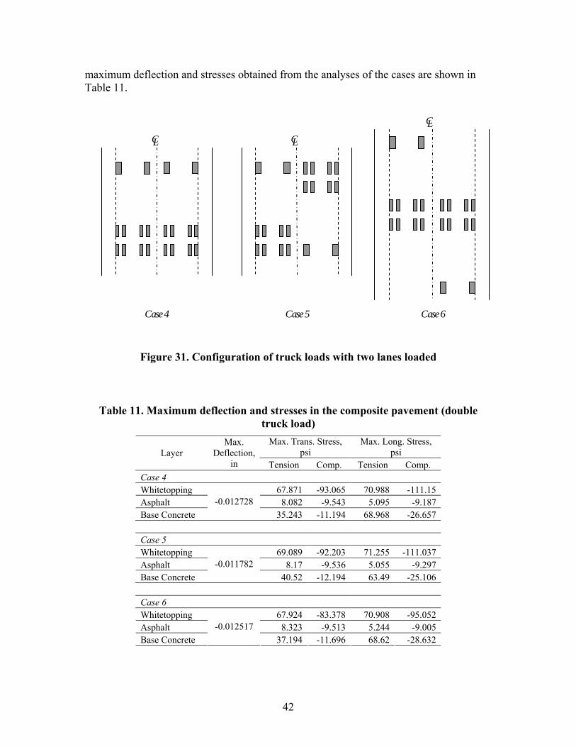
maximum deflection and stresses obtained from the analyses of the cases are shown in Table 11.

CL CL CL

Case 4 Case 5 Case 6

Figure 31. Configuration of truck loads with two lanes loaded

Table 11. Maximum deflection and stresses in the composite pavement (double truck load)

Layer Max.

Deflection, in

Max. Trans. Stress, psi

Tension Comp.

Max. Long. Stress, psi

Tension Comp. Case 4 Whitetopping Asphalt -0.012728

67.871 8.082

-93.065 -9.543

70.988 5.095

-111.15 -9.187

Base Concrete 35.243 -11.194 68.968 -26.657

Case 5 Whitetopping Asphalt -0.011782

69.089 8.17

-92.203 -9.536

71.255 5.055

-111.037 -9.297

Base Concrete 40.52 -12.194 63.49 -25.106

Case 6 Whitetopping Asphalt Base Concrete

-0.012517 67.924

8.323 37.194

-83.378 -9.513

-11.696

70.908 5.244 68.62

-95.052 -9.005

-28.632

42

Generally, the cases where the truck loads were placed side-by-side yielded the highest stresses. While the stresses for Cases 4 and 5 were not always higher than that obtained by the single truck in Case 1, longitudinal tensile stresses were approximately twice that of Case 1. In addition, the maximum contact stress in the plane of the interface elements for the cases investigated above were less than 80 psi, obtained from the whitetopping– ACC interface in the edge loading case (Case 3). This was again much less than the bond strength values presented in the construction report (Cable et al. 2003).

As the loading in Case 5 induced the highest tensile stresses in the whitetopping layer, a final analysis was performed by placing the outer wheels for two trucks at the edges of the pavement, positioned side-by-side and facing opposite directions, similar to the orientation in Case 5. The results from this analysis considering this load configuration hereafter referred to as Case 7. The results are summarized in Table 12.

Table 12. Maximum deflection and stresses due to worst case loading of the composite pavement

Max. Trans. Stress, psi

Max. Long. Stress, psiLayer

Max. Deflection,

in Tension Comp. Tension Comp. Case 7 Whitetopping 99.525 -86.779 173.324 -191.823 Asphalt 3.896 -29.246 2.826 -16.486 Base Concrete

-0.027157 14.630 -64.866 62.937 -26.608

As can be seen, the use of two truck loading placed on the edge of the pavement induced the highest transverse stresses in the composite pavement, while the longitudinal stresses were not significantly different from the case with a single truck loading on the pavement edge (Case 3). The maximum in-plane contact stress for this case was found to be a little less than 70 psi, occurring at the whitetopping–ACC interface.

Pavement Behavior When Subjected to Temperature Differential

The behavior of the composite pavement when subjected to temperature differentials was considered separately. As material non-linearities and large deflections were not considered in the course of this study, superposition of the results from static load and temperature analyses would sufficiently represent the effects of these two loading conditions on the pavement.

In order to investigate the effects of temperature differentials on the composite pavement on Iowa Highway 13, the composite pavement developed and presented in chapter “Modeling of Iowa Highway 13 Composite Pavement” was subjected to two temperature gradients that produced upward and downward curling of the pavement. The two gradients were +22.5°F at the top and -16.2°F at the bottom, as illustrated in Figure 32. These gradients were the maximum gradients that were obtained from temperature gage recordings from the 5 test sites on Iowa Highway 13.

43

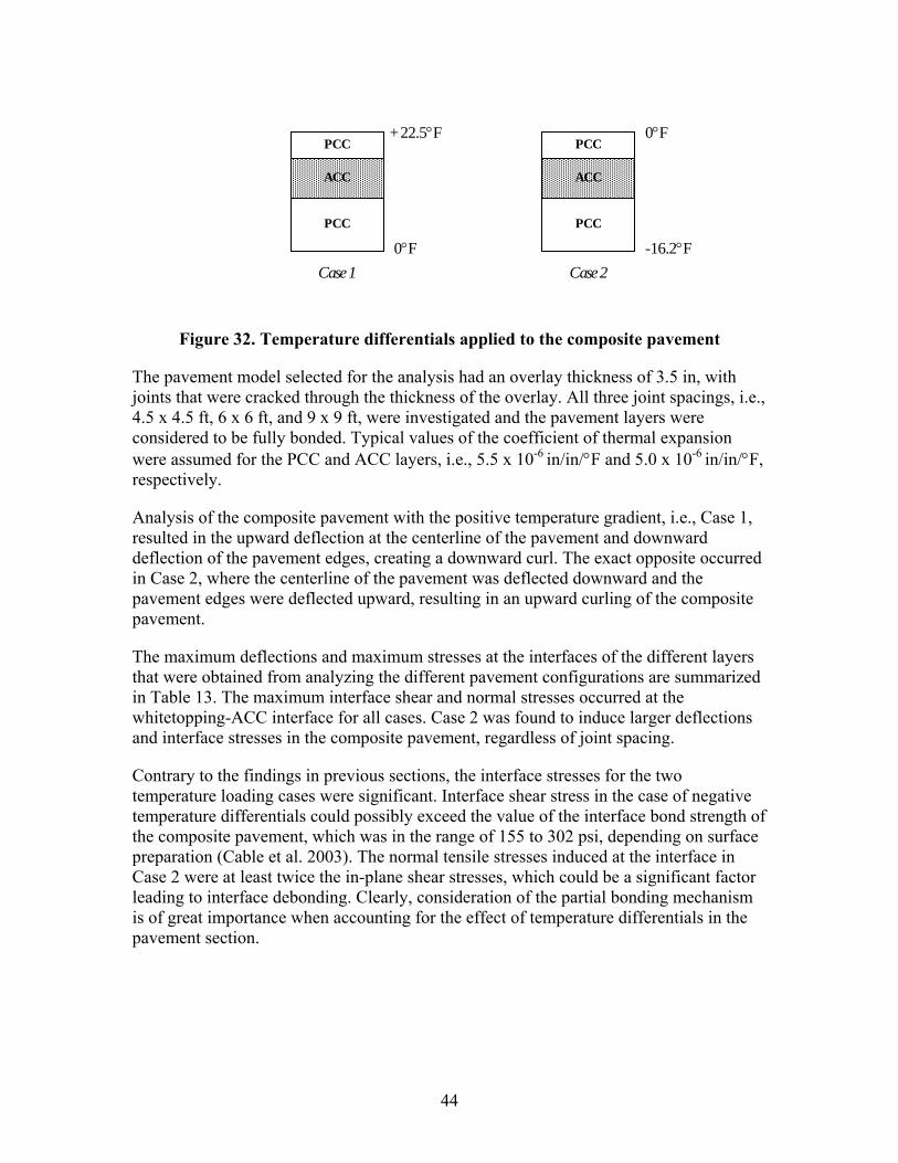
PCC

ACC

PCC

+22.5°F PCC

ACC

PCC

0°F

0°F -16.2°F Case 1 Case 2

Figure 32. Temperature differentials applied to the composite pavement

The pavement model selected for the analysis had an overlay thickness of 3.5 in, with joints that were cracked through the thickness of the overlay. All three joint spacings, i.e., 4.5 x 4.5 ft, 6 x 6 ft, and 9 x 9 ft, were investigated and the pavement layers were considered to be fully bonded. Typical values of the coefficient of thermal expansion were assumed for the PCC and ACC layers, i.e., 5.5 x 10-6 in/in/°F and 5.0 x 10-6 in/in/°F, respectively.

Analysis of the composite pavement with the positive temperature gradient, i.e., Case 1, resulted in the upward deflection at the centerline of the pavement and downward deflection of the pavement edges, creating a downward curl. The exact opposite occurred in Case 2, where the centerline of the pavement was deflected downward and the pavement edges were deflected upward, resulting in an upward curling of the composite pavement.

The maximum deflections and maximum stresses at the interfaces of the different layers that were obtained from analyzing the different pavement configurations are summarized in Table 13. The maximum interface shear and normal stresses occurred at the whitetopping-ACC interface for all cases. Case 2 was found to induce larger deflections and interface stresses in the composite pavement, regardless of joint spacing.

Contrary to the findings in previous sections, the interface stresses for the two temperature loading cases were significant. Interface shear stress in the case of negative temperature differentials could possibly exceed the value of the interface bond strength of the composite pavement, which was in the range of 155 to 302 psi, depending on surface preparation (Cable et al. 2003). The normal tensile stresses induced at the interface in Case 2 were at least twice the in-plane shear stresses, which could be a significant factor leading to interface debonding. Clearly, consideration of the partial bonding mechanism is of great importance when accounting for the effect of temperature differentials in the pavement section.

44

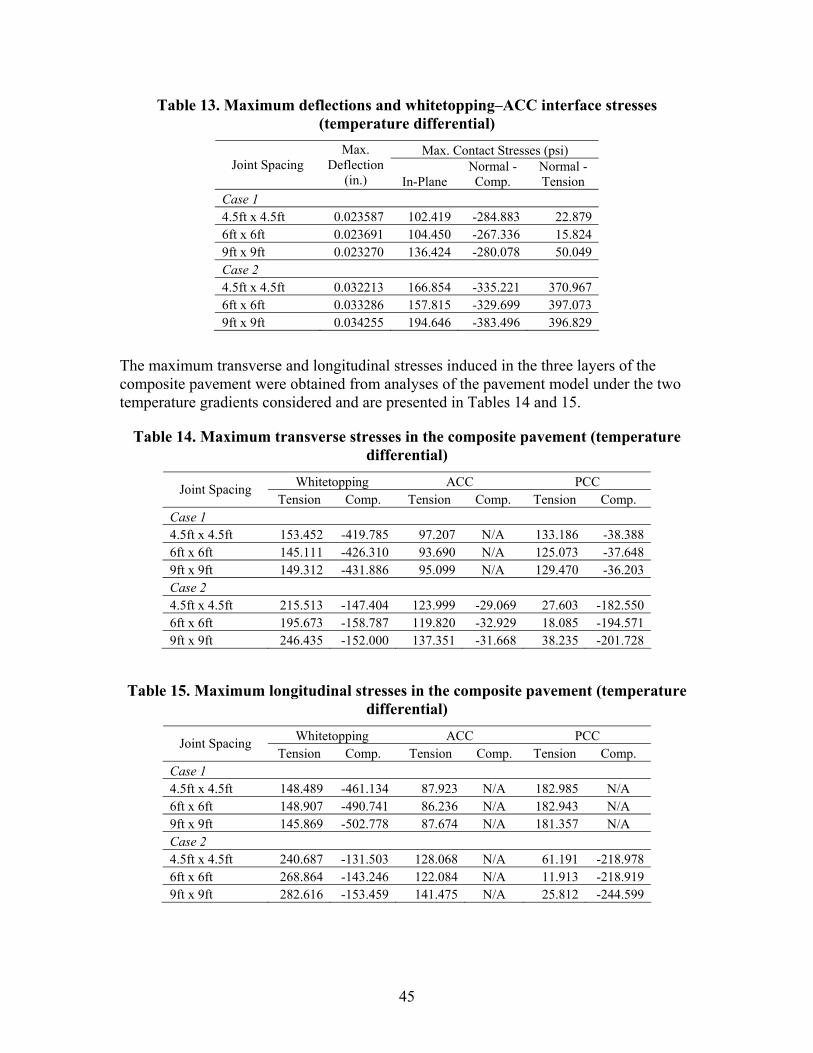
Table 13. Maximum deflections and whitetopping–ACC interface stresses (temperature differential)

Joint Spacing Max.

Deflection Max. Contact Stresses (psi)

Normal - Normal - (in.) In-Plane Comp. Tension

Case 1 4.5ft x 4.5ft 0.023587 102.419 -284.883 22.879 6ft x 6ft 0.023691 104.450 -267.336 15.824 9ft x 9ft 0.023270 136.424 -280.078 50.049 Case 2 4.5ft x 4.5ft 0.032213 166.854 -335.221 370.967 6ft x 6ft 0.033286 157.815 -329.699 397.073 9ft x 9ft 0.034255 194.646 -383.496 396.829

The maximum transverse and longitudinal stresses induced in the three layers of the composite pavement were obtained from analyses of the pavement model under the two temperature gradients considered and are presented in Tables 14 and 15.

Table 14. Maximum transverse stresses in the composite pavement (temperature differential)

Joint Spacing WhitetoppingTension Comp.

ACC Tension Comp.

PCC Tension Comp.

Case 1 4.5ft x 4.5ft 153.452 -419.785 97.207 N/A 133.186 -38.388 6ft x 6ft 145.111 -426.310 93.690 N/A 125.073 -37.648 9ft x 9ft 149.312 -431.886 95.099 N/A 129.470 -36.203 Case 2 4.5ft x 4.5ft 215.513 -147.404 123.999 -29.069 27.603 -182.550 6ft x 6ft 195.673 -158.787 119.820 -32.929 18.085 -194.571 9ft x 9ft 246.435 -152.000 137.351 -31.668 38.235 -201.728

Table 15. Maximum longitudinal stresses in the composite pavement (temperature differential)

Joint Spacing WhitetoppingTension Comp.

ACC Tension Comp.

PCC Tension Comp.

Case 1 4.5ft x 4.5ft 148.489 -461.134 87.923 N/A 182.985 N/A 6ft x 6ft 148.907 -490.741 86.236 N/A 182.943 N/A 9ft x 9ft 145.869 -502.778 87.674 N/A 181.357 N/A Case 2 4.5ft x 4.5ft 240.687 -131.503 128.068 N/A 61.191 -218.978 6ft x 6ft 268.864 -143.246 122.084 N/A 11.913 -218.919 9ft x 9ft 282.616 -153.459 141.475 N/A 25.812 -244.599

45

These results demonstrate that the stresses induced in the composite pavement by temperature differentials could be several times those induced by vertical loads. While the stresses induced in Case 1 were not significantly different in the pavements with different joint spacing, differences in stresses due to the different joint spacing used were more pronounced in the case of the negative temperature gradient. The joint spacing of 9 x 9 ft generally resulted in larger stresses in the different layers, particularly in the whitetopping overlay, which is to be expected as shorter joint spacings have been shown to reduce curling stresses (Tarr, Sheehan, and Okamoto 1998).

Once again, the assumption that the underlying layers are undamaged and crack-free might have contributed to the relatively small differences found between the different joint spacings, as the pavement behavior was essentially monolithic. One may expect larger differences between the stresses in pavements with different joint configurations as joint crack depth propagates through the thickness of the pavement section.

As the contact stresses indicate a high possibility of debonding of the three pavement layers, attempts were made to predict the stresses and deflections of the pavement model with the layers unbonded. The interface element behavior was set to “standard” to allow for separation of the layers as well as sliding, as differential curling of the different layers was expected due to the distribution of the temperature gradients.

While test runs with smaller, discrete composite panels successfully modeled the differential curling of smaller, discrete composite panels, convergence difficulties were encountered when modeling the unbonded behavior of the full pavement model developed in this study. In the author’s opinion, the complexity of the expected solution due to the combination of irregular geometry, multiple contact pairs with “standard” interface behavior, and the applied temperature gradients could have contributed to the non-convergence. Due to the lack of time, this portion of the study was not pursued further.

46

PART II—OVERLAY DESIGN METHODOLOGY

There are a number of existing design procedures that have been or could be used for whitetopping overlay design. At least four different design procedures have been identified in the literature, including those developed by the states of Colorado (Tarr et al. 1998; Sheehan et al. 2004) and New Jersey (SWK Pavement Engineering 1998), the Portland Cement Association (Wu et al. 1998) and the American Association of State Highway and Transportation Officials (AASHTO), or the American Concrete Pavement Association method (American Concrete Pavement Association 1998). Some of the more advanced procedures that have been recently developed include the modified American Concrete Pavement Association (ACPA) procedure (Riley et al. 2005) and the Total Systems Analysis Approach (The Transtec Group 2005) for design of whitetopping pavements. A review of some of these design procedures is presented in the following section.

Literature Review of Existing Methods

ACPA/PCA Ultra-Thin Whitetopping Design Guidelines

In 1998, the Portland Cement Association (PCA) and American Concrete Pavement Association (ACPA) sponsored a research study to develop thickness design guidelines for ultra-thin whitetopping (UTW) pavements (Wu et al. 1998). As part of the PCA/ACPA study, thin slabs (2 to 4 in.) with short joint spacings (24 to 50 in.) located at the Spirit of St. Louis Airport in Chesterfield, Missouri, were instrumented with strain gages and loaded using a 20 kip single axle load (SAL). The ultra-thin whitetopping test results indicated that the slab corner was the critical ultra-thin whitetopping load location, and the critical location inducing maximum asphalt strain occurred at the midpoint of the longitudinal joint.

The effects of whitetopping concrete and asphalt interface partial bonding were quantified using the PCA/ACPA study field testing results. Measured field load-induced flexural stresses were compared to fully bonded theoretical stresses to determine an adjustment factor increasing modeled ultra-thin whitetopping load stresses due to the partially bonded condition. A factor of 1.36 (36% increase in stress due to partial bonding) was determined based on the field data. This adjustment factor was applied to stresses computed during a parametric study to convert and adjust modeled stresses to simulate measured field behavior.

Linear regression techniques were then used to develop prediction equations for the ultra­thin whitetopping section critical stresses. The equations included parameters of the whitetopping pavement that have a significant impact on the induced concrete flexural stresses and asphalt flexural strains. The PCA/ACPA design procedure was developed as a guide for determining the Portland cement concrete (PCC) thickness necessary for ultra-thin whitetopping applications in low-volume traffic situations such as intersections, streets, and off ramps.

47

The development of the UTW design procedure involved the following steps (Riley et al. 2005):

1. Verify the 3-D finite element model by comparing the predicted stresses with the load testing results from the Spirit of St. Louis test pavements.

2. Characterize the degree of bond in the field and correlate that with additional load carrying capacity offered by the asphalt layer.

3. Correlate stresses predicted by the 3-D model and the 2-D model so that the 2-D model could be used to make multiple runs, thereby taking less time.

4. Develop design guidelines: a. Compute load and temperature stresses using the 2-D model under a wide

range of parameters b. Convert the 2-D stresses to 3-D stresses based on the correlation in Step 3 c. Increase the 3-D stresses by 36 percent to account for the partially bonded

condition observed in the field d. Calculate and tabulate both stresses and strains for UTW pavements under

different loading and temperature conditions e. Obtain a desired UTW pavement design by limiting both the concrete and

asphalt stresses with safe limits given a certain amount of traffic and environmental loadings over the pavement’s life

The design parameters and material properties required to determine stresses and strains for a design include the following:

• Concrete thickness (in) • Joint spacing/slab size (in) • Concrete flexural strength (psi) • Concrete modulus of elasticity (psi) • Asphalt thickness (in) • Asphalt modulus of elasticity (psi) • Composite modulus of subgrade reaction (psi) • Temperature differential between top and bottom of concrete (°F) • Coefficient of thermal expansion (CTE) of the concrete (in/in/°F) • Axle load distribution (weights and numbers of axles by type—single, tandem) • Average daily truck traffic (ADTT) • Design life (years) • Fatigue relationship (number of load applications vs. stress ratio)

The PCA/ACPA design method is technically an analysis procedure that allows for the prediction of the number of loads to fatigue failure for a given UTW configuration (Wu et al. 1998). The models used are mechanistic-empirical in nature. Initially, the concrete thickness and joint spacing (slab size) are selected. The procedure then uses these inputs together with other inputs to calculate fatigue of the PCC at the corner of the UTW and fatigue at the bottom of the Hot Mix Asphalt (HMA) under joint loading. Temperature effects are also considered. The final design is reached through an iterative (or trial and error) process.

48

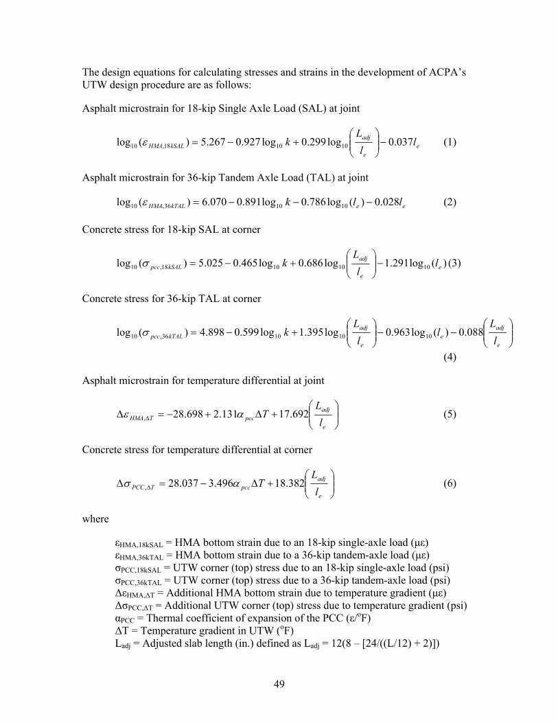
The design equations for calculating stresses and strains in the development of ACPA’s UTW design procedure are as follows:

Asphalt microstrain for 18-kip Single Axle Load (SAL) at joint

log10 (ε HMA,18kSAL ) = 5.267 − 0.927 log10 k + 0.299log10

⎛⎜⎜

Ladj ⎞⎟⎟ − 0.037le (1)

⎝ le ⎠

Asphalt microstrain for 36-kip Tandem Axle Load (TAL) at joint

log10 (ε HMA,36kTAL ) = 6.070 − 0.891log10 k − 0.786log10 (le ) − 0.028le (2)

Concrete stress for 18-kip SAL at corner

log10 (σ pcc,18kSAL ) = 5.025 − 0.465log10 k + 0.686log10

⎛⎜⎜

Lladj ⎞⎟⎟ −1.291log10 (le ) (3)

⎝ e ⎠

Concrete stress for 36-kip TAL at corner

log10 (σ pcc,36kTAL ) = 4.898 − 0.599log10 k + 1.395log10 ⎜⎜⎛ Ladj

⎟⎟⎞ − 0.963log10 (le ) − 0.088⎜⎜

⎛ Ladj ⎟⎟⎞

⎝ le ⎠ ⎝ le ⎠ (4)

Asphalt microstrain for temperature differential at joint

Δε HMA,ΔT = −28.698 + 2.131α pcc ΔT +17.692⎜⎜⎛ Ladj

⎟⎟⎞

(5)⎝ le ⎠

Concrete stress for temperature differential at corner

Δσ PCC ,ΔT = 28.037 − 3.496α pcc ΔT +18.382⎛⎜⎜

Ladj ⎞⎟⎟ (6)

⎝ le ⎠

where

εHMA,18kSAL = HMA bottom strain due to an 18-kip single-axle load (με) εHMA,36kTAL = HMA bottom strain due to a 36-kip tandem-axle load (με) σPCC,18kSAL = UTW corner (top) stress due to an 18-kip single-axle load (psi) σPCC,36kTAL = UTW corner (top) stress due to a 36-kip tandem-axle load (psi) ΔεHMA,ΔT = Additional HMA bottom strain due to temperature gradient (με) ΔσPCC,ΔT = Additional UTW corner (top) stress due to temperature gradient (psi) αPCC = Thermal coefficient of expansion of the PCC (ε/oF) ΔT = Temperature gradient in UTW (oF) Ladj = Adjusted slab length (in.) defined as Ladj = 12(8 – [24/((L/12) + 2)])

49

k = Modulus of subgrade reaction (psi/in.)le = Effective radius of relative stiffness for a fully bonded system (in.)

= {Epcc * [tpcc3 / 12 + tpcc * (NA – tpcc / 2)2] / [k * (1 - µpcc

2)]+ Eac * [tac

3 / 12 + tac *( tpcc - NA + tac / 2)2] / [k * (1 - µac2)]}0.25

NA = neutral axis from top of concrete slab (in.) = [Epcc * tpcc

2 / 2 + EHMA * tHMA * (tpcc + tHMA / 2)] / [Epcc * tpcc + EHMA * tHMA] Epcc = Modulus of elasticity of the UTW PCC (psi) EHMA = Modulus of elasticity of the HMA (psi) tpcc = Thickness of the UTW PCC (in.) tHMA = Thickness of the HMA (in.) L = Actual joint spacing (in.)

For fatigue of the PCC, the PCA fatigue cracking equations (PCA 1984) are used. For a given stress-to-strength ratio (SR), the number of loads to fatigue failure (NPCC) is calculated as follows:

For SR > 0.55 Log10(N) = (0.97187 - SR) / 0.0828 (7)

For 0.45 ≤ SR ≤ 0.55 N = (4.2577 / (SR - 0.43248 ))3.268 (8)

For SR < 0.45 N = ∞

Fatigue damage of the HMA was selected as the second possible failure criterion. For this, the Asphalt Institute (1982) method was employed. The failure criterion for this method is the number of loads that produce cracking in 20% of the wheel path area. The equation is a function of the modulus of elasticity of the HMA (EHMA) in psi and the maximum strain at the bottom of the HMA layer (εHMA), as follows:

3.29 0.854⎛ 1 ⎞ ⎛ 1 ⎞

N = 0.0795 ∗⎜⎜ ⎟⎟ ∗⎜⎜ ⎟⎟ (9) HMA⎝ ε HMA ⎠ ⎝ EHMA ⎠

The accumulated damage can then be calculated by employing Miner’s Hypothesis:

LoadGroups ⎛∑ ⎜⎜ N

ni ⎟⎟⎞ ≥ 1 (10)

i=1 ⎝ i ⎠

This analysis procedure can be conducted by dividing the expected traffic loading into load groups with single and tandem axles of known weights. The number of loads to fatigue failure in both the HMA and the PCC can be calculated, and the Miner’s Hypothesis can be used to determine the fraction of the fatigue life that has been consumed. It should be noted that some of the fatigue life in the HMA may already been

50

consumed by the trafficking before the UTW overlay; therefore, there may be an initial value of fatigue damage for that failure mode.

The steps involved in the PCA/ACPA design procedure are as follows (Riley et al. 2005):

1. Determine the neutral axis (NA) and radius of relative stiffness (le). 2. Compute the load-induced concrete stresses and asphalt strains for an 18,000 lb

single-axle load (SAL) and a 36,000 lb tandem-axle load (TAL). 3. Use a linear relationship to determine the concrete stress and asphalt strain for all

other weights in the axle load distribution category. For example, if the concrete stress under the 18-kip SAL is 187 psi, then the stress under a 20-kip SAL would be (20/18) x 287 = 319 psi.

4. Compute the temperature-induced concrete stresses and asphalt strains. These values are not load-related and are the same for all axle loads and types.

5. Sum the load-induced and temperature-induced stresses and strains to get total concrete stress and total asphalt strain.

6. Conduct the fatigue analyses. For a given set of parameters, one of the two materials will govern and determine the required thickness and joint spacing. For each axle load, do the following:

a. Compute the concrete stress ratio by dividing the total stress by the flexural strength of the concrete.

b. Use the stress ratio and fatigue relationship to determine the number of allowable load applications to fatigue failure for the concrete layer.

c. Compute the percent of fatigue used. d. Sum the concrete fatigue damage for all axle loads, both single and

tandem, and determine if greater than 100 percent. e. Determine the allowable load repetitions for the asphalt layer using the

asphalt modulus of elasticity and the calculated microstrains. f. Sum the asphalt fatigue damage for all axle loads, both single and tandem,

and determine if greater than 100 percent. 7. If either asphalt or concrete fatigue is greater than 100 percent, alter the design

inputs and rerun the analysis.

The benefits and limitations of the PCA/ACPA UTW design procedure are identified in the NCHRP Synthesis 338 (2003).

Benefits

• The PCA/ACPA design procedure considers the unusual geometry and bond inherent in a UTW overlay, which is not considered in other design procedures, such as those in the AASHTO design guide (ACPA 1998).

• As the design method was developed through the use of a 3-D Finite Element (FE) analysis, it more realistically predicts the pavement responses.

• The method recognizes the importance of bonding characteristics of the UTW to the HMA layer.

• The method was validated though the use of data from a number of field sites.

51

• The design method uses multiple failure criteria, recognizing the complexity of the UTW system.

Limitations

• To account for the partial bonding between the PCC and HMA layers, a correction term (multiplier) was derived for the corner stress prediction. However, this stress multiplier is based on a single field test location, making extrapolation prone to error. In addition, the use of a constant correction factor oversimplifies the UTW pavement response under load, especially because a constant value for the HMA resilient modulus was used.

• The current design procedure does not account for reliability in the design. The only exception is an inherent reliability of the stress multiplier.

• In the current design procedure, two modes of failure govern the predicted service life: fatigue cracking at the corner of the UTW and fatigue cracking of the HMA layer beneath the UTW. Although HMA fatigue may be a contributor to UTW distress, HMA alligator cracking in the wheel path, as the model used currently predicts, does not apply, owing to the differences in geometry and loading.

• The developers state that for UTW pavements, “the asphalt layer is covered by concrete slabs, and pavement rutting would not be the governing distress.” However, from observations of UTW overlays in service, this mode of failure does appear to be significant, and it should possibly be considered.

• The procedure contains the requirements for a number of inputs that may be difficult to define accurately by the typical user, including, for example, a “design temperature differential.”

• The current fatigue relationship included in the PCA design method yields results at a high reliability level. However, lower type facilities, such as local roads and city streets, for which UTW was originally conceived for, are designed using reliability levels between 75 and 80 percent. This is less than the in-built reliability in the PCA models. Thus, applying the PCA models will result in excessive UTW thickness, and this makes them less suitable for UTW design (Riley et al. 2005).

Colorado Thin Whitetopping Design Procedure

The State of Colorado was interested in using thin whitetopping as a technique for rehabilitating deteriorated asphalt highway pavements and, therefore, wanted to adopt the PCA/ACPA whitetopping design procedure. However, the PCA/ACPA design procedure did not include concrete thicknesses and joint spacings Colorado state officials considered acceptable for the highway projects being considered for whitetopping rehabilitation. Therefore, research was initiated to develop thin whitetopping design guidelines for the State of Colorado.

The Colorado Department of Transportation (CDOT) rationale for developing a thin whitetopping design procedure that incorporates stress correction factors was primarily to

52

take advantage of the partial bonding phenomenon between the concrete and asphalt layers. This would allow the DOT to construct the most economical whitetopping pavements possible and increase the feasibility of thin whitetopping as a rehabilitation technique for asphalt pavements.

Therefore, in 1996, the Colorado Department of Transportation and Portland Cement Association co-sponsored and initiated a research project to develop a mechanistic design procedure for thin whitetopping pavements (Silwferbrand 1997). This project involved construction of three TWT pavements containing many test sections with field instrumentation. TWT sections from 5 to 7 in. thick, with joint spacings of up to 12 ft, were instrumented to measure critical stresses and strains as a result of traffic loads and temperature differentials. Construction Technology Laboratories, Inc. (CTL) installed the instrumentation, conducted the load testing on the instrumented test sections, performed a theoretical analysis, and developed a thin whitetopping design procedure for CDOT. Many variables were considered in the construction of the test sections, including concrete overlay thickness, slab dimension, existing asphalt layer thickness, different asphalt surface preparation techniques, and the use of dowel and tie bars.

The general techniques used in the development of the PCA/ACPA ultra-thin whitetopping design procedure were also used to develop the original Colorado guidelines. Field testing was conducted to evaluate critical load locations for the thicker PCC layer and larger joint spacings. The load-induced flexural strains were used to calibrate fully bonded stresses computed using finite element analysis techniques with partially bonded stresses measured in the field. Load testing was also conducted throughout the course of a day to develop temperature corrections for the load responses. Equations predicting the critical concrete flexural stresses and asphalt concrete strains for use in whitetopping design were developed, and thickness design guidelines were established for partially bonded thin whitetopping pavements using field calibrated theoretical stresses.

In addition to the Colorado mechanistic thin whitetopping design procedure originally developed in 1998 (based on an axle load distributions obtained from traffic monitoring data), the Colorado Department of Transportation also requested that the procedure be converted so that the empirical theory of Equivalent Single Axle Loads (ESALs) could be used as the traffic input information (Sheehan et al. 2004). This required extrapolating AASHTO axle load conversion factors to include typical thin whitetopping thicknesses because the AASHTO design procedure does not suggest conversion factors for a pavement thickness below 6 in. Two ESAL conversion factors were developed based on actual traffic data (for Primary and Secondary Highways) supplied by CDOT for 8 in. thick conventional pavements. In addition to ESAL conversion factors, a nonlinear relationship was realized for PCC thicknesses determined using the empirical (ESAL) and mechanistic (axle load) procedures. An additional conversion factor was derived to equilibrate the empirical and mechanistic design methods.

The development of guidelines for bonded whitetopping during the original 1998 study (Tarr et al. 1998) and the subsequent verification and revision of the design guidelines (Sheehan et al. 2004) included the following elements:

53

1. The critical load location for the design of whitetopping pavement was determined and verified by comparing the stress data collected for each load position.

2. Critical load-induced stresses were determined when there was approximately a zero temperature gradient.

3. An analysis of experimental and theoretical concrete stresses was made (no temperature gradient). The calibration factor originally developed to adjust theoretical fully bonded stresses to measured partially bonded concrete stresses was revised.

4. An adjustment factor originally developed to convert theoretical fully bonded maximum asphalt flexural strains to partially bonded strains was revised.

5. To account for loss of support with temperature curling effects, an equation was originally derived and presently reviewed that incorporates the percent change in stress (from zero temperature gradient) based on the unit temperature gradient (°F/in.).

6. The calculation of design concrete flexural stress and asphalt strain for a specific set of design parameters involves the following steps:

• Maximum load-induced concrete stresses and asphalt strains were computed for fully bonded whitetopping pavements using the finite element program ILSL2 (Khazanovich and Ioannides 1993). A wide range of pavement parameters and material properties were originally covered, but additional ILSL2 analyses were performed and incorporated into the current study.

• Stepwise least squares linear regression techniques were used to derive the original equations to predict concrete stresses and asphalt strains from different pavement parameters and material properties. These equations have been re-derived and the new equations presented based on the 2004 study (Sheehan et al. 2004).

• Theoretical load-induced concrete stresses are increased to account for the partially bonded condition (step 3 above).

• Theoretical load-induced asphalt strains are decreased to account for the partially bonded condition (step 4 above).

• The increased load-induced concrete stresses are adjusted to account for loss of support with temperature curling effects (step 5 above).

7. Whitetopping concrete thicknesses are established by limiting both the concrete flexural stresses and asphalt flexural strains within safe limits under anticipated traffic and environmental conditions during the pavement’s design life. The procedure uses fatigue concepts to evaluate the concrete and asphalt layers separately. Therefore, for a given set of pavement parameters and material properties, the concrete or the asphalt layer may govern the design.

In this design procedure, the location of critical stress is hypothesized as being centered along a longitudinal free edge joint, such as a PCC curb and gutter. Because the joints loaded by traffic will most likely not be in a free edge condition, the design procedure considers tied longitudinal joints. The relationship between the free edge stress and tied edge stress is given as follows:

54

σFE = 1.87 * σTE (11)

where σFE is the longitudinal free joint load-induced stress (psi) and σTE is the load-induced stress at a longitudinal tied joint (psi).

Comparison of the theoretical stresses with the measured tied edge loading stresses showed that the measured stresses are greater than the theoretical stresses. The correction factors are reported as follows:

1998 Original Model (Tarr et al. 1998)

σex = 1.65 * σth (12)

2004 Adjusted Model (Sheehan et al. 2004)

σex = 1.51 * σth (13)

where σex is the measured experimental partially bonded interfacial stresses and σth is the theoretical fully bonded interfacial stresses.

To assess the PCC-HMA interface, the strains were measured in the top of the HMA pavement and also in the bottom of the PCC slab in the field. It was found that the strain in the HMA is less than the strain in the PCC pavement, which is the result of slippage between the layers. The equations representing the loss of strain are as follows:

1998 Original Model (Tarr et al. 1998)

εac = 0.842 * εpcc (14)

2004 Adjusted Model (Sheehan et al. 2004)

εac = 0.897 * εpcc - 0.776 (15)

where εac is the strain in the HMA surface and εpcc is the strain in the PCC bottom.

Once the theoretical load-induced stresses are adjusted for the partial bonding condition, the effect of the temperature-induced curling is applied. The relationship derived between the change in stress and measured temperature gradient is as follows:

1998 Original Model (Tarr et al. 1998)

σ% = 4.56 * ∆T (16)

55

2004 Adjusted Model (Sheehan et al. 2004)

σ% = 3.85 * ∆T (17)

where σ% is the percent change in stress from zero temperature gradient and ∆T is the temperature gradient (oF/in.).

For the corner and tied edge loading conditions, the following combinations of parameters were investigated for single and tandem axle configurations, resulting in nearly 4000 ILLI-SLAB (ILSL2) analysis runs being performed:

• Joint spacing, L: 48, 72, and 144 in. • Concrete slab thickness, tpcc: 4, 5, 6, and 7 in. • Asphalt layer thickness, tac: 3, 6, and 9 in. • Concrete modulus of elasticity, Epcc: 4 million psi • Asphalt modulus of elasticity, Eac: 0.05, 0.25, 0.5, 0.75, and 1 million psi • Concrete Poisson's ratio, µpcc: 0.15 • Asphalt Poisson's ratio, µac: 0.35 • Modulus of subgrade reaction, k: 50, 150, 300, and 500 psi/in. • Truck axle configuration: single (SAL) and tandem (TAL) • Slab loading locations: corner and longitudinal edge

As a result of this analysis, design equations were developed for the prediction of PCC stresses from both 20-kip single-axle loads and 40-kip tandem-axle loads. Similar equations were also developed for the HMA strain. All of these equations depend on the effective radius of relative stiffness for the fully bonded slabs. Adjustments are made to the stress equations to account for partial bond and the loss of support as a result of temperature-induced curling. Since the single-axle load concrete stress prediction model developed during the original study (Tarr et al. 1998) does not appear to provide satisfactory predictions of the modeled stresses, revised equations were developed in 2004 (Sheehan et al. 2004). The original and redeveloped prediction equations for computing design concrete flexural stresses and asphalt flexural strains are listed below:

1998 Original Model (Tarr et al. 1998)

Concrete stress for 20-kip SAL

σpcc = 919 + 18,492 / le - 575.3 log k + 0.000133 Eac

(R2adj. = 0.99) (18)

Concrete Stress for 40-kip TAL

σpcc = 671.2 - 0.000099 Eac - 437.1 log k + 1.582 * 104 / le

(R2adj. = 0.99) (19)

56

Asphalt Strain for 20-kip SAL

1/εac = 8.51114 * 10-9 Eac + 0.008619 le/L (R2

adj. = 0.99) (20)

Asphalt Strain for 40-kip TAL

1/εac = 9.61792 * 10-9 Eac + 0.009776 le/L (R2

adj. = 0.99) (21)

2004 Revised Model (Sheehan et al. 2004)

Concrete stress for 20-kip SAL

1/ 2 −6(σ pcc ) = 18.879 + 2.918(t pcc tac )+ 425.44 / le − 6.955x10 Eac − 9.0366 log k + 0.0133L (R2

adj. = 0.91) (22)

Concrete Stress for 40-kip TAL

1/ 2 −6(σ pcc ) = 17.669 + 2.668(t pcc t ac )+ 408.52 / le − 6.455x10 Eac − 8.3576log k + 0.00622L

(R2adj. = 0.92) (23)

Asphalt Strain for 20-kip SAL

1/ 4 −7(ε ac ) = 8.224 − 0.2590(t pcc tac )− 0.04419le − 6.898x10 Eac −1.1027 log k (R2

adj. = 0.81) (24)

Asphalt Strain for 40-kip TAL

1/ 4 −7(ε ac ) = 7.923 − 0.2503(t pcc tac )− 0.04331le − 6.746x10 Eac −1.0451log k (R2

adj. = 0.82) (25)

where

σpcc = maximum stress in the concrete slab, psi εac = maximum strains at bottom of asphalt layer, microstrain Epcc = concrete modulus of elasticity, assumed 4 million psi Eac = asphalt modulus of elasticity, psi tpcc = thickness of the concrete layer, in. tac = thickness of the asphalt layer, in. µpcc = Poissons ratio for the concrete, assumed 0.15

57

µac = Poissons ratio for the asphalt, assumed 0.35 k = modulus of subgrade reaction, pci le = effective radius of relative stiffness for fully bonded slabs, in.

= {Epcc * [tpcc3 / 12 + tpcc * (NA – tpcc / 2)2] / [k * (1 - µpcc

2)] + Eac * [tac

3 / 12 + tac *( tpcc - NA + tac / 2)2] / [k * (1 - µac2)]}0.25

NA = neutral axis from top of concrete slab, in. = [Epcc * tpcc

2 / 2 + Eac * tac * (tpcc + tac / 2)] / [Epcc * tpcc + Eac * tac] L = joint spacing, in.

Both PCC and HMA fatigue relations were used as failure criteria in this procedure. The PCA fatigue criterion (PCA 1984) based on Miner’s hypothesis was incorporated for PCC fatigue. This PCC fatigue criterion is as follows:

For SR > 0.55 Log10(N) = (0.97187 - SR) / 0.0828 (26)

For 0.45 ≤ SR ≤ 0.55 N = (4.2577 / (SR - 0.43248 ))3.268 (27)

For SR < 0.45 N = ∞

where SR is flexural stress-to-strength ratio and N is the allowable number of load repetitions.

The HMA pavements are generally designed based on two criteria: asphalt concrete fatigue and subgrade compressive strain to control pavement rutting. According to the developers, pavement rutting should not be the governing distress in whitetopping pavements since concrete slabs cover the asphalt layer in whitetopping pavements. Therefore, HMA fatigue was used as the design criterion in developing the Colorado design procedure. For the HMA fatigue, the number of allowable loads is a function of the maximum tensile strain in the HMA layer, the HMA modulus of elasticity, and the volume of binder and air voids. The amount of fatigue damage that the HMA has sustained before whitetopping construction is also considered. The asphalt concrete fatigue equation developed by the Asphalt Institute (1981) was employed in the development of the whitetopping design procedure. The HMA fatigue equation is as follows:

N = C * 18.4 * (4.32 X 10-3) * ( 1/ εac)3.29 * (1 / Eac)0.854 (28)

where N = number of load repetitions for 20% or greater AC fatigue cracking εac = maximum tensile strain in the asphalt layer Eac = asphalt modulus of elasticity, psi C = correction factor = 10M

58

M = 4.84 * [(Vb / (Vv + Vb) - 0.69] Vb = volume of asphalt, % Vv = volume of air voids, %

The following concerns were identified after a subsequent review of Colorado whitetopping design procedure (NCHRP 2003):

• TWT overlay thickness is substantially dependent on the subgrade modulus of reaction (k).

• TWT thickness is also sensitive to the HMA stiffness and thickness. It was stated in the procedure that the thickness of the HMA layer should not be less than 5 inches.

• TWT thickness is not sensitive to the number of 18-kip ESALs for greater than 1 million applications. However, when the loads increase, the stiffness of the HMA becomes a more significant factor. For traffic loading greater than 4 million ESALs, TWT should not be specified if the HMA modulus is less than 400 ksi.

• No guidance is provided on the proper selection of the design temperature gradient.

• The 2004 revised thin whitetopping design procedure is more sensitive than the original procedure to existing pavement subgrade characteristics, asphalt properties, and future traffic volumes. There does not appear to be specific minimum values for subgrade support or asphalt thickness necessary (as was the case for the original study).

• Due to the sensitivity of the revised thin whitetopping procedure to design procedure input parameter values, it is critical to evaluate and quantify the existing pavement conditions (i.e., subgrade support, existing asphalt modulus and thickness, remaining asphalt concrete fatigue life, anticipated traffic volumes and distributions) to get a realistic estimate of required whitetopping thickness using the revised design procedure.

Illinois (Riley et al. 2005)

Illinois first researched the experimental use of whitetopping in 1998 with the construction of three intersection projects (Winkelman 2005). Since those first three intersections, the process has been used on several more state maintained intersections and highways, as well as numerous local agency roadways and privately owned facilities. According to Pavement Technology Advisory-Whitetopping-PTA-M4 (Eff. 8/2000, Rev. 02/2005), the Illinois Department of Transportation (IDOT) has not adopted a standard design procedure for developing whitetopping overlay thickness.

In the PCA/ACPA UTW design procedures, the development of the original models for PCC fatigue included utilization of the existing fatigue relations developed by PCA (1984). According to Riley et al. (2005), the underlying assumptions in the PCA fatigue models result in an unstated, conservative factor of safety in all UTW designs developed using this procedure. In other words, the use of PCA fatigue curve imparts very high

59

levels of design reliability compared to those normally used for the design of local and secondary roads for which UTW was originally intended. An effort was undertaken to incorporate probabilistic concepts into the existing fatigue models (Riley et al. 2005). Approximate comparisons were made with several existing projects constructed in Illinois as a base of reference for the revised models.

To select an appropriate methodology for incorporating reliability into fatigue relationships, several studies from the literature were reviewed. It was found that a methodology proposed by McCall (1958) for incorporating probability of failure or survival into fatigue analysis and predictions of N was successfully applied in several studies. The relationship proposed by McCall is as follows:

log N = ⎡⎢− SR −α log(1− p)⎤

⎥

γ

(29) ⎣ β ⎦

where N is the number of load repetitions, SR is stress ratio, p is the probability of failure and 1-p is the probability of survival, and α, β, and γ are regression constants. The methodology proposed by McCall (1958) was judged to be most appropriate and formed the basis for incorporating reliability into fatigue predictions in the model developed by Riley et al. (1995).

The first step in model development consisted of assembling data from various sources. The data elements of interest for model development were applied stress, PCC strength at testing, stress ratio, the number of load applications to failure, and information indicating whether the test specimen failed at the time testing was terminated. Data for analysis were obtained from the ACPA and several published reports and literature.

The calibration of the selected model using the assembled data consisted of the following steps:

1. Group the fatigue data into categories of SR 2. For each SR category, perform survival analysis and determine the probability of

survival of a PCC beam subjected to fatigue at the prescribed stress ratio level 3. Assemble a database of probability of survival and N for the categories of SR

established. 4. Perform nonlinear regression using the data obtained in step 3 to determine model

coefficients for the selected N prediction model (Equation 29). 5. Verify the tentative model, modify as needed, and determine final model

coefficients.

The result of the calibration effort was the development of a tentative model as follows:

⎡− SR −10.24 log(1− p) ⎤0.217

log N f = ⎢ ⎥ (30) ⎣ 0.0112 ⎦

60

The model statistics were as follows:

• N = 87 • R2* = 91 percent (R2 computed from predicted and measured logN = 91%) • RMSE = 0.31

The model verification consisted of reviewing the diagnostic statistics and conducting a sensitivity analysis. A comparison of the model developed during this study and other past studies with the current PCA model indicated that predicted log Nf from the PCA model is the most conservative.

Since the fatigue data upon which the original design procedure and the revised procedure incorporating reliability are based is essentially similar, the same limitations to interpretation apply. In order to obtain a comparison of the results, several calculations were completed using the old procedure.

Using the existing fatigue relationship, the maximum number of loads the section could carry until fatigue capacity of the concrete or the asphalt was reached was calculated. Next, analyses were completed at 90% and 95% reliability using the new fatigue relationship to contrast that with the prior model based on the old fatigue relationship. As expected, at 90% reliability, several of the calculated loads for given conditions were less conservative than those associated with the published fatigue curve, whereas at 95% reliability, the loads are, in general, more conservative (Riley et al. 2005).

The results from the revised procedure were then compared with field experience. A number of whitetopping and UTW pavements have been built in Illinois. Since the results from this analysis are based largely on theoretical concepts, an attempt was made to compare results from the revised procedure with results obtained from the IDOT projects in Illinois. By using the new models with parameters typical of Illinois and converting an ACPA category B traffic distribution to ESALs, a rough comparison was made to see if the pavements are performing at least as well as might be forecast using the revised procedure at a 90% level of reliability (ACPA 2002). Additional comparisons were completed using the data published from the Federal Highway Administration’s (FHWA) accelerated loading facility (ALF) test results (ACPA 2003).

Results from the projects considered generally indicated that all of the designs reviewed with the limited information available would meet the above criteria; though, it may be somewhat early to tell for all of the sections. The data from the ALF testing is more certain and meets the aforementioned criteria. Other conventional whitetopping projects in Illinois were not considered since they fall outside the normal limits of UTW of 2 to 4 in. The models were not developed for that range, but may later be reviewed for possibility of extrapolation to infer likely performance.

It is noted that no attempt has been made to address the fatigue of the asphalt in the paper by Riley et al. (2005). For many of these analyses, failure in the asphalt layer drove the maximum number of loads carried. It was suggested by the authors that the asphalt

61

fatigue relationship remains unchanged and warrants further study if an overall probabilistic relationship is desired. In its present form, the developed procedure allows some degree of assurance against failure by fatigue of the concrete when constructed as a UTW overlay.

Transtec Overlay Design

The Transtec Group, under sponsorship from the Innovative Pavement Research Foundation (IPRF), is currently developing a new state-of-the-art design procedure for whitetopping pavements. Employing a Total Systems Analysis Approach, the development of the new design procedure began with an in-depth study of the various failure modes that could develop in all classes of whitetopping. This approach includes the means not only to optimize the design thickness, but also to optimize other key variables such as the joint spacing, mix design, and surface preparation technique. A brief description of the upcoming whitetopping design guidelines is presented here.

This approach employs 18 unique steps, illustrated in Figure 33. Each cell in this figure is described below. The end result of this approach is the ability to make a side-by-side comparison of various alternatives which, using conventional design techniques, could not be accomplished.

Step 1—User Inputs

In the first step, the various user inputs are defined under seven categories: (1) general, (2) materials, (3) geometry, (4) environment, (5) traffic, and (6) economic. Each of these categories contains a number of variables that can be defined by the user. The developers acknowledge that a balance must be made between the accuracy of the software and the complexity of the inputs.

Step 2—Strategy Selection

Once the user has identified the various inputs, the strategies to be analyzed must be defined. Traditional pavement design tools will often only provide a single result— minimum thickness required to achieve a specified performance based on a small number of criteria. However, this design system is a systems analysis tool. This type of tool has the flexibility to provide the user with much more power to make the types of decisions that are critical during the pavement design.

Step 3—Loop over Each Strategy

The software tool that implements this design guide will begin the analysis by looping over each selected strategy. For example, if three different strategies were selected, the program will run three times.

62

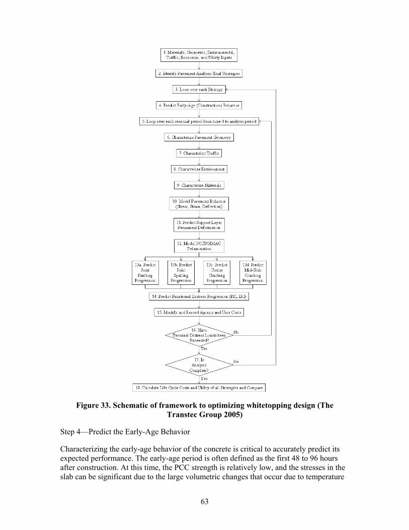
Figure 33. Schematic of framework to optimizing whitetopping design (The Transtec Group 2005)

Step 4—Predict the Early-Age Behavior

Characterizing the early-age behavior of the concrete is critical to accurately predict its expected performance. The early-age period is often defined as the first 48 to 96 hours after construction. At this time, the PCC strength is relatively low, and the stresses in the slab can be significant due to the large volumetric changes that occur due to temperature

63

and moisture conditions in the slab. This is especially true for UTW slabs due to the high surface area to volume ratio. Algorithms from the FHWA HIPERPAV™ analysis tool will be selected to predict the early-age behavior.

Step 5—Loop over Each Seasonal Period

This step includes one of the characterizing elements of this unique approach. The essence of a systems analysis tool is to predict the various paving strategies as realistically as possible. This simulation is done in a chronological fashion by looping over each season from the initial construction season up to the last season of the user- defined analysis period. During this simulation, the various distresses will be predicted incrementally, and the resulting performance can then be derived from this distress history. Unlike traditional design tools, the process described here has the flexibility to compare various strategies side-by-side.

Step 6—Characterize Pavement Geometry

Using the various user inputs, the geometry of the pavement system is characterized in this step. This primarily involves characterizing the various layer thicknesses, so it is relatively straightforward.

Step 7—Characterize Traffic

The traffic for the current period is defined in this step. Adjustments to the traffic are made as follows:

• Axle-load spectra. The simulation will be performed over the full range of anticipated axle-load spectra. An integration of the number of axles by the distress due to each axle load will be made to predict the overall incremental distress.

• Seasonal distribution of traffic. For example, higher traffic may be experienced during the summer months on some facilities; therefore, an adjustment is made to reflect this effect.

• Growth. The traffic level will generally increase with time. An adjustment will be made to reflect the growth function as defined by the user. Three growth functions are provided—linear, exponential, and logistic (s-shaped) growth.

• Time of day. The simulation also loops over the time of day. This effect is important since the deflected shape of the pavement will differ from day to night, and therefore will impact the predicted traffic-induced stresses. The user can define either a functional class or an hourly traffic distribution to better define the traffic volumes during different times of the day.

Step 8—Characterize Environment

Various user inputs are needed to characterize the ambient environmental conditions at the specified location for the design. In order to minimize the burden to the user, these inputs will be made using a sophisticated GIS-based interface. When a location for the

64

design is selected, an extensive 600-megabyte database is queried for weather data from weather stations in the vicinity of the specified location.

Using an intelligent algorithm, the most relevant weather stations are selected, and the weather information for the specified location is calculated based on a weighted interpolation scheme. The database actually contains mean hourly readings for the entire year (based on 30 years of data) for each of the specified stations. For simplicity, these values are reduced seasonal means. In addition, the database contains the variances for each of these factors in order to better characterize the stochastic nature of weather phenomena.

Using the ambient environmental inputs along with the materials inputs, the temperature profiles in the pavement system will be predicted using a finite-difference algorithm, similar to that of the Integrated Climate Model (ICM) developed for the FHWA. The remaining characterization, behavior, and distress models in the systems analysis, in turn, will use these profiles.

Step 9—Characterize Materials

Contrary to most pavement design methods, the key properties of paving materials to predict pavement performance are not static values. Although, most design procedures simplify the characterization of materials properties such as modulus and strength, the systems analysis approach to pavements does not require this assumption to be made. This is quite beneficial since most of the key properties are a function of dynamic variables such as temperature, moisture, cumulative damage, and time.

For example, the software will use two unique models to predict the concrete strength and modulus. The first model is based on maturity methods and would be used during the early-age analysis (Step 4), and the second model is based on a more general form and would be used for subsequent analysis period (Step 9).

Step 10—Model Pavement Behavior

Pavement behavior modeling is a controversial issue—primarily among academia, but also among practitioners who are simply asking for the “right answer.” Over the years, many models have been developed to predict the responses of a pavement system due to both environmental and traffic loading. Regarding whitetopping, pavement responses of interest include the following:

• Critical stresses in the whitetopping layer—corner stresses and edge stresses • Deflections and strains in the whitetopping layer at the corner and the edge • Stresses and strains in the HMA support layer • Stresses and strains in the base and subgrade layers • Delamination stresses and strains (which will be covered in more detail in step

12).

65

Coming up with the “right answer” is quite difficult, however. The types of models range widely. On one extreme are simple closed-form solutions such as those developed by Westergaard and refined by Bradbury in the early part of last century. On the other extreme are dynamic, non-linear three-dimensional finite element prediction models. One trade-off between these models, and everything in between, is run-time versus accuracy.

Closed-form solutions may be easy to program and implement into a system such as this, but their accuracy is limited due to the simplicity of the inputs and the inherent assumptions. Three-dimensional finite element models, on the other hand, require tremendous computing power and are beyond reasonable feasibility at this time for integration into the systems analysis tool during run-time. The Transtec Group project team believes that it will provide the "best of both worlds" in the current approach.

The response model will be a hybrid “2½D” model consisting of a non-linear two- dimensional (2-D) finite element model foundation. This model will be modified via simplified correction models developed using a non-linear three-dimensional (3-D) FEM.

Step 11—Predict Support Layer Permanent Deformation

In thinner whitetopping pavements, failures that have been observed are often caused, either directly or indirectly, by a loss of support due to permanent deformations in the support layers. In some cases, the permanent deformation is in the HMA layer directly beneath the whitetopping. In other pavements, the failure may be in the base, or even in the subgrade.

Predicting the progression of permanent deformations in the support layers accurately is a key element in the overall systems analysis approach. This prediction model will set up the boundary conditions necessary to predict the response of the whitetopping layer in subsequent periods.

Step 12—Model Whitetopping-HMA Delamination

Whitetopping layers are traditionally designed and analyzed based on the assumption that a bond exists between the concrete and the HMA layers. However, a number of factors contribute to the deterioration of the bond between these layers:

• Upward warping of the slab corners and edges due to moisture loss from the top portion of the PCC slab

• Upward curling of the slab corners and edges due to negative temperature gradients in the PCC slab

• Axial shrinkage of the slab due to drying shrinkage • Axial shrinkage or expansion of the slab due to changes in slab temperature • Traction forces caused by passing wheel loads • Dynamic forces of passing wheel loads • Shrinkage of the support layers due to moisture changes • Permanent deformation of the support layers • Swelling of the support layers

66

• Healing of the HMA • Relaxation creep in the PCC slab

The characterization and, furthermore, the interaction of these variables is quite complex. However, many of these parameters can be modeled and will be incorporated into the systems analysis.

The bond between the HMA and the concrete layers must resist delamination forces. A state of stress can be modeled at the interface using a number of models. To compare to this predicted stress, two “strengths” must be considered:

1. The bond strength of the interface between the HMA and the PCC layers 2. The strength of the HMA, considering factors such as the loading rate, stress state,

and temperature.

The weakest of these strengths will govern the delamination of the layers.

Step 13—Model Whitetopping Structural Distresses

From the observations of the project team, four key structural distresses have noted to be predominant in whitetopping pavements to date. These include the following distresses:

• Joint Faulting—the vertical separation of adjacent slabs that is due to many factors, including poor load transfer and loss of support.

• Joint Spalling—a localized failure along a joint where pieces of PCC have failed and broken away from the slab. There are two primary sources of spalling distress—deflection-related and delamination-related. The former is caused by high deflections in the slab that create high shear stresses in the top layer of the slab at the joint, resulting in a localized failure. Delamination spalling is often caused by significant moisture loss from the slab resulting in weak horizontal planes, which then fail under subsequent traffic loading.

• Corner Cracking—a cracking failure in the vicinity of the slab corner. • Mid-Slab Cracking—a cracking failure that occurs in the middle of a slab. This

type of cracking can occur due to either high volumetric changes in the PCC, coupled with high restraint, or by fatigue due to repeated traffic loading.

Step 14—Predict Functional Distress Progression in Whitetopping

Although the prediction of structural distresses is a key factor in a mechanistic-based analysis system, it is highly recommended that a means to predict the functional distress also be provided. The two primary indicators in use today to quantify the functional distress are the Present Serviceability Index (PSI) and the International Roughness Index (IRI).

67

Step 15—Identify and Record Agency and User Costs

At the end of the analysis cycle, the agency and user costs will be calculated for the current period. The former requires little modeling—only a good "bookkeeping" routine that will accrue the construction costs to the agency. The user costs, however, require a more sophisticated model. This model will account for the traffic volumes, time of day of the maintenance, and other items which relate to the impact to the traffic.

Step 16—Check to see if Distress Limits have been Exceeded

This step will conduct an evaluation of the current state of the pavement. If the simulation has predicted a level of distress that the user denotes as being "terminating" in nature, the analysis will complete. This, in essence, allows the analysis period to be shortened to eliminate analysis options that do not meet the basic minimum criteria set by the user.

As an extreme example, if a one-inch whitetopping is selected for construction over an HMA of poor condition subjected to very heavy traffic loading, it will intuitively not reach an analysis period of 15 years. In this case, the program will drop out of the analysis when the maximum terminating level of distress is exceeded. It is also at this point that the loop completes to advance to the next season to be simulated. As mentioned in step 5, each strategy will be simulated over the analysis period as defined by the user.

Step 17—Check to see if Analysis is Complete

If each of the strategies that the user had selected for the systems analysis has been executed and simulated, the analysis will terminate. If not, the analysis will continue to loop through to the next strategy.

Step 18—Calculate and Compare Life-Cycle Costs for all Strategies

This step includes the use of sophisticated life-cycle cost analysis (LCCA) techniques to predict values that can immediately be used by the user to compare the alternative strategies.

A comparison of the whitetopping design procedures discussed in this section is made in Table 16.

68

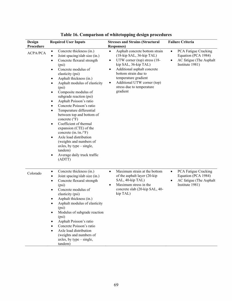
Table 16. Comparison of whitetopping design procedures Design Required User Inputs Stresses and Strains (Structural Failure Criteria Procedure Responses)

ACPA/PCA • Concrete thickness (in.) • Joint spacing/slab size (in.) • Concrete flexural strength

(psi) • Concrete modulus of

elasticity (psi) • Asphalt thickness (in.) • Asphalt modulus of elasticity

(psi) • Composite modulus of

subgrade reaction (psi) • Asphalt Poisson’s ratio • Concrete Poisson’s ratio • Temperature differential

between top and bottom of concrete (°F)

• Coefficient of thermal expansion (CTE) of the concrete (in./in./°F)

• Axle load distribution (weights and numbers of axles, by type – single, tandem)

• Average daily truck traffic (ADTT)

• Asphalt concrete bottom strain (18-kip SAL, 36-kip TAL)

• PCA Fatigue Cracking Equation (PCA 1984)

• UTW corner (top) stress (18­kip SAL, 36-kip TAL)

• AC fatigue (The Asphalt Institute 1981)

• Additional asphalt concrete bottom strain due to temperature gradient

• Additional UTW corner (top) stress due to temperature gradient

Colorado • Concrete thickness (in.) • Joint spacing/slab size (in.) • Concrete flexural strength

(psi) • Concrete modulus of

elasticity (psi) • Asphalt thickness (in.) • Asphalt modulus of elasticity

(psi) • Modulus of subgrade reaction

(psi) • Asphalt Poisson’s ratio • Concrete Poisson’s ratio • Axle load distribution

(weights and numbers of axles, by type – single, tandem)

• Maximum strain at the bottom • PCA Fatigue Cracking of the asphalt layer (20-kip Equation (PCA 1984) SAL, 40-kip TAL) • AC fatigue (The Asphalt

• Maximum stress in the Institute 1981) concrete slab (20-kip SAL, 40­kip TAL)

69

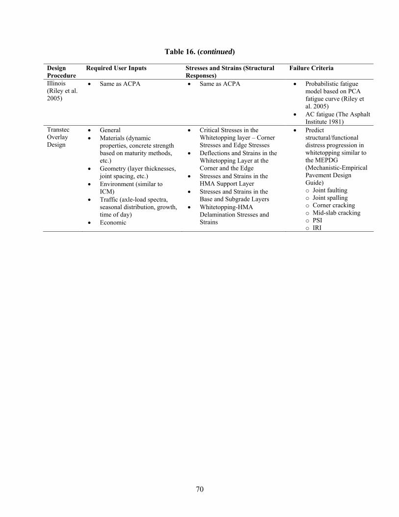
Table 16. (continued)

Design Required User Inputs Stresses and Strains (Structural Failure Criteria Procedure Responses) Illinois • Same as ACPA • Same as ACPA • Probabilistic fatigue (Riley et al. model based on PCA 2005) fatigue curve (Riley et

al. 2005) • AC fatigue (The Asphalt

Institute 1981) Transtec • General Overlay • Materials (dynamic Design properties, concrete strength

based on maturity methods, etc.)

• Geometry (layer thicknesses, joint spacing, etc.)

• Environment (similar to ICM)

• Traffic (axle-load spectra, seasonal distribution, growth, time of day)

• Economic

• Critical Stresses in the Whitetopping layer – Corner Stresses and Edge Stresses

• Deflections and Strains in the Whitetopping Layer at the Corner and the Edge

• Stresses and Strains in the HMA Support Layer

• Stresses and Strains in the Base and Subgrade Layers

• Whitetopping-HMA Delamination Stresses and Strains

• Predict structural/functional distress progression in whitetopping similar to the MEPDG (Mechanistic-Empirical Pavement Design Guide) o Joint faulting o Joint spalling o Corner cracking o Mid-slab cracking o PSI o IRI

70

Mechanistic Whitetopping Thickness Design Procedure

The Colorado DOT (CDOT) thin whitetopping procedure and the Portland Concrete Association (PCA) ultra-thin whitetopping procedure both outline methods for designing a thin concrete overlay on top of an existing Asphaltic Concrete (AC) pavement. However, many of the roads in Iowa and other states consist of Portland Cement Concrete (PCC) pavements overlaid with AC. This is done in order to extend the service life of the pavement. This section outlines a process to evaluate the existing pavement conditions and determine the parameters required to apply the CDOT and PCA design procedures.

Evaluation of the Existing Pavement

To evaluate the existing conditions of the composite (AC/PCC) pavement, visual inspection and deflection testing should be conducted. Deflection testing is performed with a FWD and load magnitude of 9000 pounds. The deflection testing should be done in enough intervals that will allow for an adequate evaluation of the pavement. Measurements taken from sensors, located at 0, 12, 24, and 36 inches from the center of the load plate, are adjusted for temperature effects on the AC moduli and standardized for a load of 9000 lbs. These results are used to compute the maximum deflection (d0) and the deflection basin AREA. The parameters or layer moduli of the existing AC/PCC pavement are then backcalculated using the two values (Hall and Darter 1994).

Temperature Effects

In order to account for temperature effects during load testing, temperature of the AC layer must be monitored. An alternative method to determine the temperature of the AC using the mean monthly air temperature was developed by Witczak and is shown below (Asphalt Institute 1982).

T = MMAT ⎛1 + 1 ⎞

⎟ − 34

+ 6 (31) ac ⎜⎝ z + 4 ⎠ z + 4

where

Tac = mean temperature of the asphalt layer MMAT = mean monthly air temperature z = 1/3 depth from the surface of the asphalt, inches

Asphalt Modulus

A large portion of the total deflection can be attributed to the vertical compression of the AC layer under the 9000 lb load. To determine the amount of compression in the asphalt, the AC elastic modulus needs to be calculated. The method outlined below uses the Asphalt

71

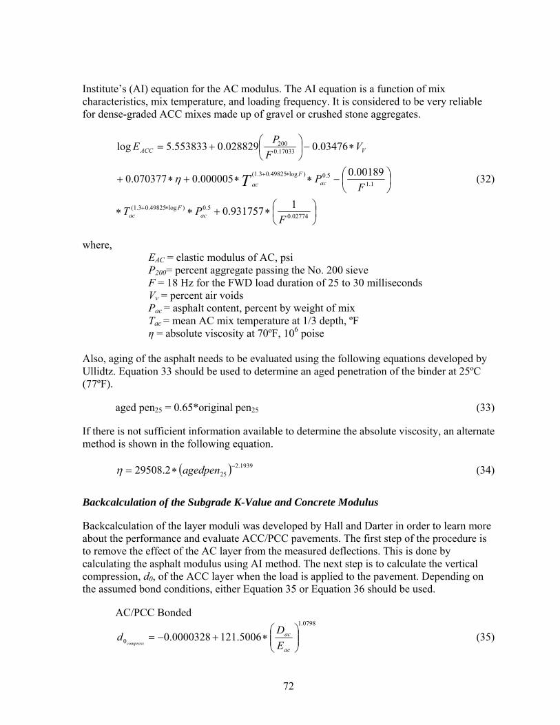
Institute’s (AI) equation for the AC modulus. The AI equation is a function of mix characteristics, mix temperature, and loading frequency. It is considered to be very reliable for dense-graded ACC mixes made up of gravel or crushed stone aggregates.

⎛ P200 ⎞log EACC = 5.553833 + 0.028829⎜ 0.17033 ⎟ − 0.03476 ∗VV⎝ F ⎠

(1.3+0.49825∗log F ) 0.5 − ⎛ 0.00189 ⎞+ 0.070377 ∗η + 0.000005 ∗T ac ∗ Pac ⎜ 1.1 ⎟ (32)

⎝ F ⎠

∗T (1.3+0.49825∗log F ) ∗ P0.5 + 0.931757 ∗⎛⎜ 1 ⎞

⎟ac ac 0.02774⎝ F ⎠

where, EAC = elastic modulus of AC, psi P200= percent aggregate passing the No. 200 sieve F = 18 Hz for the FWD load duration of 25 to 30 milliseconds Vv = percent air voids Pac = asphalt content, percent by weight of mix Tac = mean AC mix temperature at 1/3 depth, ºF η = absolute viscosity at 70ºF, 106 poise

Also, aging of the asphalt needs to be evaluated using the following equations developed by Ullidtz. Equation 33 should be used to determine an aged penetration of the binder at 25ºC (77ºF).

aged pen25 = 0.65*original pen25 (33)

If there is not sufficient information available to determine the absolute viscosity, an alternate method is shown in the following equation.

η = 29508.2 ∗ (agedpen25 )−2.1939 (34)

Backcalculation of the Subgrade K-Value and Concrete Modulus

Backcalculation of the layer moduli was developed by Hall and Darter in order to learn more about the performance and evaluate ACC/PCC pavements. The first step of the procedure is to remove the effect of the AC layer from the measured deflections. This is done by calculating the asphalt modulus using AI method. The next step is to calculate the vertical compression, d0, of the ACC layer when the load is applied to the pavement. Depending on the assumed bond conditions, either Equation 35 or Equation 36 should be used.

AC/PCC Bonded 1.0798

⎛ D ⎞acd = −0.0000328 + 121.5006 ∗⎜⎜ ⎟⎟ (35) 0compress ⎝ Eac ⎠

72

AC/PCC Unbonded 0.94551

⎛ D ⎞acd0 = −0.00002132 + 38.6872 ∗⎜⎜ E ⎟⎟ (36) compress

⎝ ac ⎠

where d0 compress = AC compression at center of load, in Dac = AC thickness, in Eac = AC elastic modulus, psi

After the compression of the AC layer at the center of the load is calculated, this value is subtracted from the maximum deflection (d0) measured by the FWD in order to find the deflection of the PCC layer.

d0PCC = d0 − d0compress (37)

where d0 compress = vertical compression of the AC layer, in d0 = maximum deflection at center of load plate, in d0PCC = deflection of the PCC layer, in

Now that the asphalt layer has been accounted for, the procedure follows regular backcalculation techniques:

1. Calculate the area of the deflection basin under PCC slab using the d0 calculated above and the d12, d24, and d36 measured at the AC surface.

AREAPCC = 6 ∗⎛⎜⎜1 + 2 ∗

⎛⎜⎜ d

d12 ⎞⎟⎟ + 2 ∗

⎛⎜⎜ d

d24 ⎞⎟⎟ +

⎛⎜⎜ d

d36 ⎞⎟⎟⎞⎟⎟

(38) PCC PCC⎝ ⎝ 0 ⎠ ⎝ 0PCC ⎠ ⎝ 0 ⎠⎠

where AREAPCC = area of the deflection basin, in d0PCC = deflection of the PCC layer at center of load plate, in di = deflection at distance i from the center of the load plate, in

2. Calculate the radius of relative stiffness (l).

⎡ ⎛ 36 − AREAPCC ⎞⎤4.387

l = ⎢⎢ ln

⎝⎜ 1812.279 ⎠

⎟⎥⎥

(39) ⎢ − 2.559 ⎥ ⎢ ⎥⎦⎣

73

3. Calculate the L/l. L is the least slab dimension divided by l calculated in #2.

4. The above backcalculation procedure uses Westergard’s equation for deflection of an infinite plate on a dense liquid foundation. However, many slabs are too small to approximate infinite slab behavior. Therefore if the L/l resulting value is less than eight, the following corrections must be performed to the maximum deflection and radius of relative stiffness.

−0.66914∗⎛⎜ L ⎞⎟

0.84408

AFd = 1 −1.0687 ∗ e ⎝ l ⎠ (40) 0

−2.17612∗⎜⎛ L ⎞⎟

0.49895

AFl = 1 − 5.29875 ∗ e ⎝ l ⎠ (41)

adjusted d0 = AFd0 ∗ measured d0 (42)

adjusted l = AFl ∗ calculated l (43)

5. Calculate the k-value using Westergard’s deflection equation.

⎛ P ⎞⎧⎪ ⎛ 1 ⎞⎡ ⎛ a ⎞ ⎤⎛ a ⎞2 ⎫⎪k =

⎝⎜⎜ 8 ∗ d0 ∗ l 2

⎠⎟⎟⎩⎪⎨1 +

⎝⎜ 2π ⎠

⎟⎣⎢ln

⎝⎜ 2 ∗ l ⎠

⎟ + γ −1.25 ⎦⎥⎝⎜ l ⎠

⎟⎭⎪⎬ (44)

where k = effective modulus of subgrade reaction, pci (dynamic) d0 = adjusted maximum deflection d0, in l = adjusted radius of relative stiffness P = FWD load, pounds γ = Euler’s constant, 0.57721566490 a = load radius, 5.9 inches for the FWD

6. Using the definition of l and dividing the k-value by two, the concrete elastic modulus may be determined.

2 412 ∗(1 − μ )∗ k ∗ lEPCC = PCC (45) 3DPCC

74

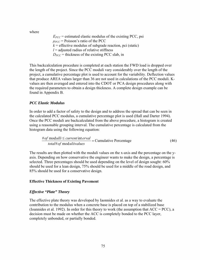
where EPCC = estimated elastic modulus of the existing PCC, psi μPCC = Poisson’s ratio of the PCC k = effective modulus of subgrade reaction, pci (static) l = adjusted radius of relative stiffness DPCC = thickness of the existing PCC slab, in

This backcalculation procedure is completed at each station the FWD load is dropped over the length of the project. Since the PCC moduli vary considerably over the length of the project, a cumulative percentage plot is used to account for the variability. Deflection values that produce AREA values larger than 36 are not used in calculations of the PCC moduli. K-values are then averaged and entered into the CDOT or PCA design procedures along with the required parameters to obtain a design thickness. A complete design example can be found in Appendix B.

PCC Elastic Modulus

In order to add a factor of safety to the design and to address the spread that can be seen in the calculated PCC modulus, a cumulative percentage plot is used (Hall and Darter 1994). Once the PCC moduli are backcalculated from the above procedure, a histogram is created using a reasonable grouping interval. The cumulative percentage is calculated from the histogram data using the following equation:

#of modulli ≤ current int erval = Cumulative Percentage (46)

total#of moduliivalues

The results are then plotted with the moduli values on the x-axis and the percentage on the y-axis. Depending on how conservative the engineer wants to make the design, a percentage is selected. Three percentages should be used depending on the level of design sought: 60% should be used for a lean design, 75% should be used for a middle of the road design, and 85% should be used for a conservative design.

Effective Thickness of Existing Pavement

Effective “Plate” Theory

The effective plate theory was developed by Iaonnides et al. as a way to evaluate the contribution to the modulus when a concrete base is placed on top of a stabilized base (Ioannides et al. 1992). In order for this theory to work (the assumption that ACC = PCC), a decision must be made on whether the ACC is completely bonded to the PCC layer, completely unbonded, or partially bonded.

75

Unbonded ACC and PCC Layer

If the ACC and PCC layers are not bonded, the equation to calculate thickness of the effective “plate” is rather simple.

EPCC

1 3)

PCC

(⎡ ⎤3 3Dhe D ∗ (47) +⎢⎣

= ⎥⎦

AC EAC

where he = effective thickness of the existing pavement, in DAC = thickness of the AC layer, in DPCC = thickness of the PCC layer, in EAC = elastic modulus of the AC, psi EPCC = elastic modulus of the PCC, psi

Bonded ACC and PCC Layers

If the ACC and PCC layers are bonded, then the neutral axis of the composite plate is calculated. The first step is to calculate the depth to the neutral axis (x).

DAC

2+ +

DPCC

2 ⎞⎟⎠

⎛⎜⎝

E D E D DAC AC PCC PCC ACC

(48) x =E D E DPCC+AC AC PCC

where DAC = thickness of the AC layer, in DPCC = thickness of the PCC layer, in EAC = elastic modulus of the AC, psi EPCC = elastic modulus of the PCC, psi

Next, calculate the thickness of the effective plate (he).

( )31EPCC

EAC

⎧ ⎫D3 AC + 3

PCCD⎪⎪

⎪⎪⎬he (49)

⎡⎨= 2 2 ⎤x −

DAC

2 DAC +

EPCC

EAC

⎛⎜⎝

DAC −x +DPCC

2 ⎞⎟⎠

⎛⎜⎝

⎞⎟⎠

⎪ ⎪⎩

⎪ ⎪⎭

D+12⎢⎢⎣

⎥⎥⎦

PCC

where DAC = thickness of the AC layer, in DPCC = thickness of the PCC layer, in EAC = elastic modulus of the AC, psi EPCC = elastic modulus of the PCC, psi

76

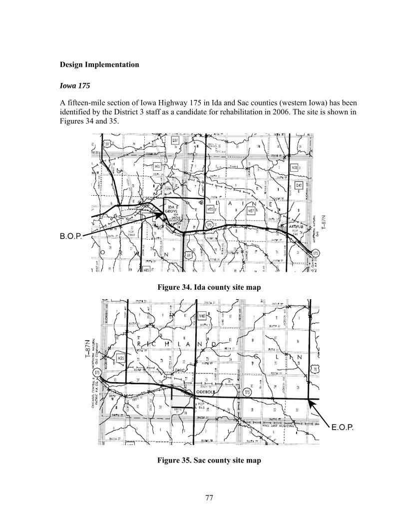
Design Implementation

Iowa 175

A fifteen-mile section of Iowa Highway 175 in Ida and Sac counties (western Iowa) has been identified by the District 3 staff as a candidate for rehabilitation in 2006. The site is shown in Figures 34 and 35.

Figure 34. Ida county site map

Figure 35. Sac county site map

77

The route consists of an existing thickened edge concrete pavement that has been widened and overlaid with Asphaltic Concrete. The original rehabilitation concepts involved various mill and fill Asphaltic Concrete options. The research team has been able to conduct field FWD deflection measurements every 0.2 mile in each direction on the project. The results of this and visual surveys of the project have been used as inputs to the previously described design procedure. The design procedure has indicated the need for a 4.5-inch PCC overlay if no bonding is assumed between the overlay and the existing ACC layer. If bond is assumed, the overlay thickness could be reduced to 3.5 inches. In each case, the pavement will be widened from 24 to 28 feet with an 8-inch deep non-tied PCC widening unit.

This work and one other project being considered in northeastern Iowa will represent the first use of this new design methodology in Iowa. These projects will represent the implementation phase of the design methodology and provide validation and upgrading of the procedure in the future for Iowa State and local road needs.

Overlay Planning Guidelines

It is important that the rehabilitation program planners and rehabilitation designers understand the locations where this specific overlay design method can be best applied. The pavement engineers should pay special attention to the following characteristics of the existing roadway cross section and condition:

1. Review of “as built” plans. The performance of this type of overlay depends heavily on the materials and condition of the underlying layers at the time of the overlay. This review will help the pavement engineer understand the visual survey performance indicators in a field review.

a. The materials used in the concrete layer at the bottom of the existing pavement should be durable. Gain an understanding of the existence of reinforcement and its layout. Is it continuous mesh, load transfer, or a bar configuration in portions of the slab?

b. Identify the transverse joint spacing and the depth of the PCC slabs. Is this a uniform depth section or thickened edge pavement, and what were the cross slopes on the surface of that layer?

c. How many ACC overlays have been placed on this slab, what was the overlay depth and date of placement, what was the material makeup, and what surface preparations were done prior to each overlay? Are the overlay materials subject to stripping or deformation? (You must conduct coring to determine the presence or absence of stripping.) Has the pavement been widened, and if so, with what type of materials and to what depth?

d. What type, amount, and location of drainage layers or systems are present along the roadway? A review of existing drainage ways adjacent to the project can identify farm tile and drainage obstructions.

78

2. Traffic Estimate. Determine the historical mix of the traffic and the number of axle loadings it has experienced from original construction to the present time. What will be the mix and volumes of various vehicle types (especially trucks or farm equipment) expected in the design period?

3. Field review of the project. This activity should involve the combined efforts of the pavement engineer, soils engineer, planner, designer, and the local maintenance supervisor at a minimum and any pavement history/management records review for the project area. This is an important step in collecting knowledge of the pavement that does not appear in written records.

a. Identify each pavement distress, frequency, and severity over the length of the project. Is the distress found throughout the project or in isolated portions? Take note of field entrances of heavy farm equipment or crossroads locations such as a quarry location near the roadway.

b. Try to determine whether the distress is load, environmental, or material related. Examples may include excessive numbers of transverse cracks that are “tented” upwards. If these cracks are associated with joints in the underlying PCC pavement, it may mean that the concrete is deteriorated to a point where the new overlay will not bridge this problem. It may also mean there is no load transfer or the reinforcement is deteriorated to a point of no practical use. If there are many transverse cracks between PCC joints, one should consider the existence of transverse steel in the concrete layer acting as another deteriorated joint. This usually results in “tenting” of the crack. If more than 20% of these are “tented” up, it is doubtful that any kind of thin overlay will perform adequately.

c. Look for longitudinal working cracks at a joint between the original pavement and the widening unit. A working crack here must be considered in the jointing plan for the overlay.

d. Determine the location of other working cracks (longitudinal, transverse, or diagonal) that will require reinforcement in the overlay.

e. Identify the location of existing full depth patches and their condition. If they have failed, this is the time to replace them. If more than 20% of the transverse joints in the project have been patched in this manner and more are needed, thin concrete overlay rehabilitation should not be considered. An unbonded overlay of significant thickness (6″ or greater) should be considered along with the option of removal and replacement of the entire roadway structure.

f. Identify areas of potential delamination in the ACC or ACC/PCC underlying pavement layers due to moisture or pavement longitudinal growth and blowups. If blowups have occurred in the past, what material was used to patch them and were moisture conditions dealt with at the site? How much additional drainage work will be required and how will it be placed relative to the existing pavement cross section?

79

g. Identify special needs for additional widening to accommodate trucks entering and leaving the pavement and navigating horizontal curves.

h. Identify special needs of the surrounding property owners that must be met during construction. Is daily access essential or can special arrangements for access be provided during construction?

i. Identify the drainage structures that must be lengthened or widened. Will bridge decks be overlaid or will the overlay be transitioned into the existing decks? Are the drainage structures in need of replacement? If so, they should be replaced and patched with a full depth before the overlay is placed.

j. Identify the need and location for any shoulder widening. The new pavement should have at least 3 foot of earth or granular shoulder outside the paved area to protect the pavement section.

k. A review of detour potential routes should be considered at this time. It is not necessary, but could speed up construction and opening to traffic.

l. Field review data collection should include the following: random coring of layers at selected distressed and good performing transverse joints, wheel paths and mid panel/quarter points to determine the stability of each layer, and potential delamination areas between various layers.

m. FWD deflection testing should be performed at each 0.2-mile location in the outer wheel path in each direction of travel on the project roadway. This amount may be reduced over time by the design agency when they develop a level of confidence in the variability along the roadway with their results. Testing should be done with a load and with sensors placed between surface cracks and not across a reflective crack.

Overlay Design Guidelines

The following items should be considered in the development of the PCC overlays.

1. Depth and condition of the various layers of the existing pavement. If the underlying PCC layer contains large amounts of steel reinforcement that is causing reflective cracking in the surface of the pavement, this pavement should not be considered for a thin PCC overlay. Treat this pavement as an in-place base and design a conventional unbonded PCC overlay of 6 inches or greater on the pavement.

If the cores taken in the field indicate debonding or delamination between the ACC layers or the ACC/PCC, interface consideration should be given to removal of the ACC to that interface. In the case the interface between the ACC/PCC is the problem, complete removal of the ACC and replacement with a one-inch ACC bond breaker should be considered to insure good performance of the new PCC overlay and to reduce the potential for reflective cracking.

2. Overlay depth should be determined from the results of the coring, deflection testing, and anticipated traffic mix and volume. It should consider the amount of ACC depth

80

being removed in the milling procedure and make allowance for the reduced composite section depth.

3. The entire ACC surface should be milled to a minimal depth that allows for the road surface crown to be restored while removing any high spots across the road surface. It is not necessary or advised to remove the ACC to the bottom of the ruts that may be present in the ACC surface. Millings can be used for shoulder materials in most cases.

Termini at bridges or ends of the project should be milled to a depth of 6 inches or greater at the junction with the existing pavement. Mill across the slab at this point to get a vertical edge at the junction of the new and old surfaces. If this means removal of some of the existing PCC, treat that section as a bonded section in terms of joint patterns. This provides a thickened end where vehicle impact loads are prevalent.

In the event the existing widening unit longitudinal joint is open and working, it is suggested that the widening unit be milled to a depth of the design widening unit and a new joint established at this point. Expansion joint material shall be replaced near bridge termini according to highway agency standards.

4. Joint patterns in the surface PCC overlay should be determined in relationship to the slab width of the underlying PCC pavement. Divide the lane width into segments that are nearly square in nature and allow for the retention of a lane or centerline joint. Either joint can become a reflective crack if not considered in the design. Joint spacing of the PCC overlay in feet should not exceed twice the depth in inches, unless fibers are used. In this case, do not exceed the instructions of the fiber manufacturer. The fibers will hold cracks tight and to some degree assist in bonding, but they will not stop the crack from forming. The object of joint design is to allow for the differences in cement chemistry of today and allow for curl and warp to occur in the thin surface without causing cracks. Care should be taken to eliminate longitudinal joints in the wheel paths wherever possible.

Evaluate the condition of the existing widening joint. If geotextile or metal reinforcement was used across the original joints in the overlay and the joint is tight, the designer can neglect this joint as a potential reflective crack in the overlay.

5. The use of fibers is suggested in PCC overlays of less than 4 inches as an insurance policy against loss of surface due to a crack. They will not stop cracking, but will retard loss of material around the crack. Research is ongoing to evaluate the use of the fibers to allow for larger joint patterns in the overlay that could match the underlying PCC layer joint pattern.

6. Tie bars across the longitudinal joints should be used in PCC depths of 6 inches or greater due to placement problems. In the case of the longitudinal joint between a new widening unit and the existing pavement, where the PCC overlay thickness is less than 3″–6″, tie bars, nailed to the existing ACC surface at 36-inch spacings should be considered.

81

7. Concrete quantities should be bid in two bid items. The first should be for volume delivered in cubic yards. Be aware that this reduces the risk to the contractor, fills the rutted areas and the overlay volume, and will often overrun between 10%-20% due to irregularities in the slab wheelpaths. The second bid item is for concrete placement by the square yard that covers the placement and finishing, curing, and texturing of the concrete as will be used in a conventional PCC new pavement construction.

8. Construction survey for the overlay should involve cross sections on 25-foot intervals and points across the slab that involve the two edges of slab, centerline of roadway, center of wheelpath (rut), and lane centerpoints as a minimum. This minimizes the potential for unexpected overrun identified in item 7. It allows the engineer to identify high points in the cross section that will affect the minimum depth in a given cross section and the longitudinal grades vs. the volume of concrete required to meet a good profile and minimum depth of concrete requirements. This also requires the paving contractor to utilize two string lines to guide his machine for each edge of the roadway.

Overlay Construction Guidelines

The construction of this type of overlay creates its own problems and solutions. With consideration of the following items, the project should move smoothly forward with little or no inconvenience for the traveling public. The goal of this work is to treat the construction process in the same manner as a conventional ACC overlay construction project. This requires that the designer and construction industry consider new paradigms in portland cement concrete pavement construction.

1. Scheduling of work items on the contract should direct the contractor to close portions of the road only when paving is ongoing. All removal items, drainage construction, and shouldering work should be done under traffic.

One of the critical considerations in this process is the location of the subdrains and their timing in the construction process. Consideration of the location relative to the edge of the existing vs. finished pavement edge is critical to the sequencing and traffic control.

2. Paving can be accomplished by either one-lane or two-lane construction techniques. The use of maturity testing for determination of strength gain and pilot car operations will allow for continuous use of the highway during one-lane construction. The rapid placement of this overlay proceeds at a pace that will allow multiple miles to be placed in one week in one direction and in the following week in the opposite direction. This process will require new ideas to protect the drop-off at the edge of the pavement for access points by public traffic during construction.

Two-lane construction can proceed at an equally fast pace if a detour is available. This method allows for a better performing longitudinal centerline joint. The maturity method of estimating concrete strength can be used with proper concrete mix

82

selection to reduce property owner inconvenience to less than 20 hours (car traffic) and construction traffic to approximately 30 hours (truck traffic) being off the placed slab.

This type of paving moves very quickly and the contractor must be prepared to not only take care of the surface area in terms of finishing, but also maintain a good surface profile. This will be the controlling activity in this type of construction.

3. The use of fibers and current texturing methods using burlap, Astroturf, and tining machines will bring some of the fibers to the surface behind the paving operation. These will not damage the pavement performance and can be removed by the first set of highway traffic or snowplow operations of the winter season.

4. Traffic control can be the same as that used on other overlay projects. It is essential that the contractor and the businesses along the project understand the construction process to be used. A preconstruction public meeting can alleviate many of the potential conflicts with deliveries and access along the project.

5. Concrete placement for this type of overlay requires that the pavement be clean of all foreign matter in front of the paving operation. This will insure the proper opportunity for bonding between the overlay and the existing surface. Temperature monitoring of the existing ACC surface should be employed to keep the surface temperature below 100 degrees Fahrenheit. In the event that temperature is exceeded, the surface should be sprayed with water to cool the surface. Excess water should be removed prior to the placement of the concrete.

6. In the event fibers are selected for introduction into the mix, the contractor should demonstrate that the introduction method will eliminate the potential for balling. The use of agitating haul units allows for the addition of the fibers at the plant and mixing during hauling. If dump trucks are used for hauling, means of blowing the fibers into the mixing drum or alternative but worker-safe modes should be demonstrated prior to beginning the work.

7. Curing and surface texturing for this type of work must remain close to the slipform paving operation due to the depth of the overlay and the changing weather conditions over the course of the day. It is recommended that multiple maturity locations be considered for each day’s placement. Research indicates that the changes in existing pavement surface temperature over the course of the day may dictate that some areas be skipped by the saw in the morning in order to meet the rapid strength gain potential that could have occurred in the middle of the afternoon.

8. Due to the small distance between joints, the joint formation should be done with early entry saws and 1/8-inch-wide blades. Joint formation in both directions should be initiated as soon as concrete strengths are in the 100 to 120 psi flexural strength range or when raveling of the joint does not occur behind the saw. Depth of joint

83

formation should be accomplished to the same relative depth as that in full-depth pavement specifications.

The process of first sawing a transverse joint in the 15- to 20-foot range of spacing and then allowing other saws to follow with the intermediate joints can prevent premature cracks on hot weather days. In the case of thin overlays, it is important to keep the longitudinal sawed joint formation closer to the slipform than on full depth pavements. It is probable and possible to keep all the joint formation operations within 1,000 to 1,500 feet of the slipform paver for mixes that do not contain slag or similar retarding type materials.

Existing Iowa research indicates no difference in joint performance between joints that were air blasted after sawing and joints that were not cleaned. The only caution is the buildup of sawing dust and its effect on profile measurements. This can be eliminated with the use of a power broom. If water is used to cool the saw blades, then water flushing of the joints should be done.

9. The owners and contractors must change their perspective on opening this road to traffic. Shouldering should be done as soon as the pavement strength allows for construction traffic. This normally will be within two days after paving and can be monitored with the maturity method of estimating concrete strength.

84

SUMMARY, CONCLUSIONS, AND RECOMMENDATIONS

Analytical study

Summary

The state of Iowa is one of the states known for their extensive PCC pavements, where the potential for cost savings from whitetopping is a very attractive alternative to continued pavement rehabilitation with asphalt. To gain further experience in the use of whitetopping for pavement rehabilitation, the state of Iowa has sponsored several research projects to test and monitor a 9.6-mile stretch of Iowa Highways 13. The following points represent the summary of the field and the analytical investigations:

• Published analytical studies have demonstrated the feasibility of utilizing the finite element method to aid in the study of pavements constructed with a concrete whitetopping overlay.

• Owing to the irregular geometry of the composite pavement on Iowa Highway 13, three-dimensional finite element models were developed using the ANSYS finite element program to aid in the investigation of the behavior of the composite pavement. Solid and shell elements were used in modeling various configurations of the pavement structure on Iowa Highway 13.

• In order to study the effects of the interface bonding between the different layers, interface elements capable of modeling bonded and unbonded interactions were utilized. In addition, beam elements were used to represent tie bars where necessary. The applicability of the modeling techniques were then tested and affirmed by comparison of the results obtained from ANSYS with beam and plate theories and by comparison with the ISLAB2000 software package.

• The applicability of the 3-D model developed in ANSYS for the composite pavement on Iowa Highway 13 was tested by comparing the results from the finite element analysis to measured deflection and strain data from the field. Deflections from the field were in good agreement with the deflections obtained from analysis. On the other hand, comparisons of analytical and measured strains were inconclusive. This could be due to various factors that could not be adequately controlled experimentally or precisely accounted for in the analytical process. However, based on the results of the deflection comparisons, the finite element models developed for the Iowa Highway 13 composite pavement were deemed adequate to further investigate the structural behavior of the pavement.

• A parametric analysis was performed in order to determine the effects of the whitetopping thickness, joint spacing, joint crack depth, interface bond, widening unit configuration, and tie bar size and spacing. In addition, temperature data collected from the field was utilized to analyze the effect of the temperature gradient on the composite pavement behavior.

85

Design Method

• The existing design methods for thin overlays contain much of the same theory and are tailored for the specific needs of the user.

• The Iowa method is designed to use tools available to the state highway department staff in the form of as-built plans, traffic projections, coring, deflection testing, and visual distress surveys to form the inputs to the design process. Much of the Colorado procedure has been incorporated into this process.

• The design process will be validated in one or more construction projects in 2006 and 2007 on state highways. The performance results do match well with existing projects on Iowa Highways 13 and 21 with their 3 and 10 years of experience, respectively.

Conclusions

• The behavior of a composite pavement with fully bonded layers, subjected to actual truckloads and temperature differentials, can be accurately predicted with the 3-D model developed with this study.

• The interface elements in the ANSYS program are suitable for modeling the fully bonded and unbonded interface conditions between the different pavement layers.

• Thicker whitetopping overlays were found to improve pavement performance by lowering deflections and maximum stresses that were induced in the composite pavement under static loading.

• Investigations into pavement behavior as a function of the different joint spacing or different crack depths demonstrate that the condition of the layers underlying the whitetopping greatly influence the behavior of the pavement. With the assumption of undamaged, crack-free base PCC and ACC layers, joint spacing and crack depth did not have a significant effect on pavement performance.

• Composite pavements with fully bonded and unbonded layers exhibited very different behavior. For example, the deflections and maximum stresses induced in pavements with unbonded layers were significantly higher than in pavements with fully bonded layers.

• The width, rather than the depth, of the widening units has a significant effect on reducing the deflection.

• Load transfer between the widening units and the composite section of the pavement section has to be maintained to reduce the deflection induced in the pavement under vertical traffic loads.

• Even in the absence of the aggregate-interlock load transfer mechanism, tie bars with reasonable size and spacing were capable of providing the aforementioned load transfer between the widening units and composite section.

• A PCC overlay design procedure has been developed based on the existing Colorado design procedure and modified to use existing information that can readily be obtained by state highway department staff.

86

• The overlay design procedure provides for acceptable performance for traffic volumes of up to 2,000 ADT and in excess of 10 years, as indicated in the Iowa Highway 21 research results.

• Thin PCC overlay and widening units do provide a viable and economical alternative in the field of overlay rehabilitation strategies for narrow highway pavements.

Future Recommendations

The following are the recommendations for further study:

• The FWD deflection data should be normalized such that the effects of variable temperatures and foundation stiffnesses may be isolated.

• The quality of the strain data obtained from the field should be improved by ensuring the integrity of the gages after installation, which can easily be attained if these gages are installed during the construction of new pavements. Also, interference from passing traffic should be eliminated during data collection.

• The non-linear material properties for both asphalt and concrete should be included to account for fundamental material behavior, such as concrete cracking or asphalt viscosity or stripping, that could influence the behavior of the pavement.

• Time factors such as concrete fatigue, creep, and shrinkage need also be incorporated into a study of pavement performance to determine any possible long-term destructive effects.

• Detailed information on the condition of the layers underlying the whitetopping is needed for the precise prediction of pavement behavior. However, this approach could be unfeasible due to the unlimited variation of actual pavement condition in the field over a relatively short length. An alternative approach could be to assume the propagation of whitetopping joints through the thickness of the pavement, with appropriate load transfer efficiency values determined by trial and error, applied between the resulting pavement panels to approximate actual pavement behavior.

• Modeling of the partial bonding condition between the different pavement layers should be an essential part of future work since this factor has a significant effect on the overall behavior and performance of composite pavements.

• The variation in the stresses at the layer interfaces could be significant when the pavement is subjected to temperature differentials. This implies that treatment of the partial bonding mechanism is of particular importance to adequately account for the effects of temperature differentials on composite pavement behavior.

• The effects of using tie bars and aggregate interlock mechanism on the load transfer between the widening units and composite section need to be further investigated.

• The behavior of the composite pavement structure under moving loads, which is a better approximation of the actual traffic loads that a pavement is subjected to during normal operation, should be investigated.

• The unbonded behavior of the composite pavement subjected to temperature differential should be investigated.

87

• Continued validation of the developed PCC overlay design process by monitoring two pavement design projects currently under development by the Iowa DOT is necessary. Also, continue to test the FWD input method with other potential projects under rehabilitation consideration.

88

REFERENCES

American Concrete Pavement Association. 1998. Whitetopping–State of the Practice. ACPA Publication EB210P. Skokie, IL: American Concrete Pavement Association

American Concrete Pavement Association. 2002. Ultrathin Whitetopping, IS100P. Skokie, IL: American Concrete Pavement Association.

American Concrete Pavement Association. 2003. Special Report–Accelerated Pavement Testing to Evaluate UTW Load-Carrying Capacity. SR002P. Skokie, IL: American Concrete Pavement Association.

ANSYS User’s Manual–Theory. 2004. ANSYS v.6.1. Canonsburg, PA: ANSYS Inc. Burnham, T., and D. Rettner. 2003. Whitetopping and Hot-Mix Asphalt Overlay Treatments

for Flexible Pavement. Maplewood, MN: Minnesota Department of Transportation. Cable, J.K., M.L. Anthony, F.S. Fanous, and B.M. Phares. 2003. Evaluation of Composite

Pavement Unbonded Overlays: Phases I and II. Ames, IA: Iowa State University, Center for Portland Cement Concrete Pavement Technology.

Cable, J.K., Professor, Iowa State University. 2004. Personal Conversation. Cook, R., D. Malkus, M. Plesha, and R. Witt. 2002. Concepts and Applications of Finite

Element Analysis, 4th Ed., John Wiley & Sons, Inc. Coree, B., Professor, Iowa State University. 2004. Electronic Correspondence. Hall, K. T., and M. I. Darter.1994. Improved Methods for Asphalt-Overlaid Concrete

Pavement Backcalculation and Evaluation. Nondestructive Testing of Pavements and Backcalculation of Moduli. Second Volume. STP 1198. Harold L. Quintus, Albert J. Bush, III, and Gilbert Y. Baladi, Eds. American Society for Testing and Materials, Philadelphia.

Huang, Y.H. 1993. Pavement Analysis and Design. Upper Saddle River, NJ: Prentice Hall. Ingram, D.N.J. 2004. The Effect of the Dowel Bar Shape and Spacing in Portland Cement

Concrete Pavements on the Load Transfer Efficiency of the Transverse Joint. Ames, Iowa: Iowa State University.

Ioannides, A. M., L. Khazanovich, and J.L. Becque. 1992. Structural Evaluation of Base Layers in Concrete Pavement Systems. Washington DC: Transportation Research Board

Khazanovich, L., and A. M. Ioannides. 1993. Finite Element Analysis of Slabs-On-Grade Using Improved Subgrade Soil Models. Proceedings, ASCE Specialty Conference: Airport Pavement Innovations–Theory to Practice. Vicksburg, MS: Waterways Experiment Station.

Kumara, W., M. Tia, C.–L. Wu, and B. Choubane. 2003. Evaluation of Applicability of Ultrathin Whitetopping in Florida. Paper presented at the annual meeting of the Transportation Research Board, Washington, DC.

McCall, J.T. 1958. Probability of Fatigue of Plain Concrete. Journal of the American Concrete Institute. vol. 30., no. 2, pp. 233-234.

National Cooperative Highway Research Program. 2002. Thin and Ultra-Thin Whitetopping. NCHRP Synthesis 338. Washington DC: Transportation Research Board, National Research Council.

National Cooperative Highway Research Program. 2003. Thin and Ultra-Thin Whitetopping. A Synthesis of Highway Practice. NCHRP Synthesis 338. Washington, DC: Transportation Research Board, National Research Council.

89

Nishizawa, T., Y. Murata, and K. Kokubun. 2003. Mechanical Behavior of Ultrathin Whitetopping Structure Under Stationary and Moving Loads. Paper presented at the annual meeting of the Transportation Research Board, Washington, DC.

Portland Cement Association. 1984. Thickness Design for Concrete Highway and Street Pavements. Engineering Bulletin No. EB-109.01P. Skokie, IL: Portland Cement Association.

Riley, R. C., L. Titus-Glover, J. Mallela, S. Waalkes, and M. Darter. 2005. Incorporation of Probabilistic Concepts into Fatigue Analysis of Ultrathin Whitetopping as Developed for the American Concrete Pavement Association. Proceedings of the International Conference on Best Practices for Ultrathin and Thin Whitetoppings. Denver, CO.

Sheehan, M. J., S. M.Tarr, and S. Tayabji. 2004. Instrumentation and Field Testing of Thin Whitetopping Pavement in Colorado and Revision of the Existing Colorado Thin Whitetopping Procedure. Report No. CDOT-DTD-R-2004-12. Denver, CO: Colorado Department of Transportation.

Silfwerbrand, J. 1997. Whitetoppings–Swedish Field Tests and Recommendations. Proceedings of the 6th International Purdue Conference on Concrete Pavement Design and Materials for High Performance. Lafayette, IN: Purdue University.

Sun-Yoong, O. 2005. Finite Element Analysis of Iowa Highway 13 Composite Pavement, Thesis, Iowa State University.

SWK Pavement Engineering. 1998. Development of a Design Guide for Ultra-Thin Whitetopping. Princeton, NJ: SWK Pavement Engineering.

Tarr, S. M., M. J. Sheehan, and P. A. Okamoto. 1998. Guidelines for the Thickness Design of Bonded Whitetopping in the State of Colorado. Report No. CDOT-DTD-R-98-10. Denver, CO: Colorado Department of Transportation.

The Asphalt Institute. 1981. Thickness Design–Asphalt Pavements for Highways and Streets. Manual Series No. 1. Lexington, KY: The Asphalt Institute.

The Asphalt Institute. 1982. Research and Development of the Asphalt Institute’s Thickness Design Manual (MS-1). Ninth Edition. Research Report 82-2.

The Transtec Group. 2005. http://www.whitetopping.com/design.asp. Voyiadjis, G.Z., P.I. Kattan. 1990. Bending of Thick Plates on Elastic Foundation. Advances

in the Theory of Plates and Shells. Studies in Applied Electromagnetics and Mechanics 24: 87-121. Amsterdam, The Netherlands: Elsevier.

Winkelman, T. J. 2005. Whitetopping Performance in Illinois. Physical Research Report No. 148. Springfield, IL: Illinois Department of Transportation.

Wu, C. L., S. M. Tarr, T. M. Refai, M. A. Nagi, and M. J. Sheehan. 1998. Development of Ultra-Thin Whitetopping Design Procedure. Portland Cement Association Research and Development Report No. 2124. Skokie, IL: Portland Cement Association.

90

APPENDIX A: STRAIN GAGE DATA

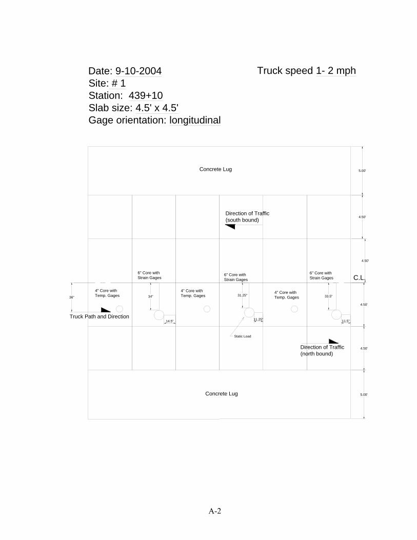
Date: 9-10-2004 Truck speed 1- 2 mph Site: # 1 Station: 439+10 Slab size: 4.5' x 4.5' Gage orientation: longitudinal

Truck Path and Direction

4" Core with Temp. Gages

6" Core with Strain Gages

4" Core with Temp. Gages

6" Core with Strain Gages

4" Core with Temp. Gages

6" Core with Strain Gages

Concrete Lug

C.L.

Concrete Lug

Direction of Traffic (south bound)

Direction of Traffic (north bound)

Static Load

5.00'

4.50'

4.50'

4.50'

4.50'

5.00'

36" 34"

14.5"

31.25"

11.25"

33.5"

11.5"

A-2

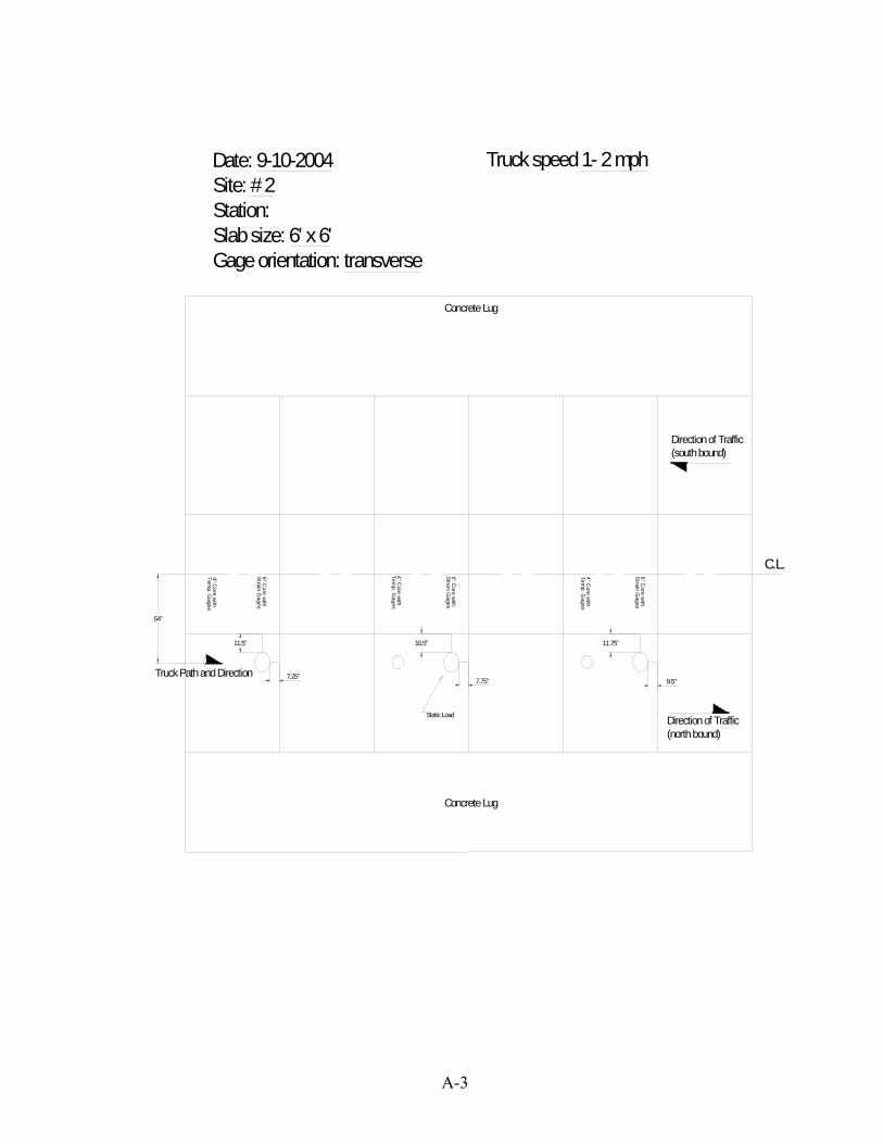
Date: 9-10-2004 Truck speed 1- 2 mph Site: # 2 Station: Slab size: 6' x 6' Gage orientation: transverse

C.L.

Concrete Lug

6" Core w

ith S

train Gages

4" Core w

ith Tem

p. Gages

4" Core w

ith Tem

p. Gages

6" Core w

ith S

train Gages

4" Core w

ith Tem

p. Gages

6" Core w

ith S

train Gages

Concrete Lug

Truck Path and Direction

Direction of Traffic (south bound)

Direction of Traffic (north bound)

11.5"

7.25"

10.5"

7.75"

11.75"

9.5"

54"

Static Load

A-3

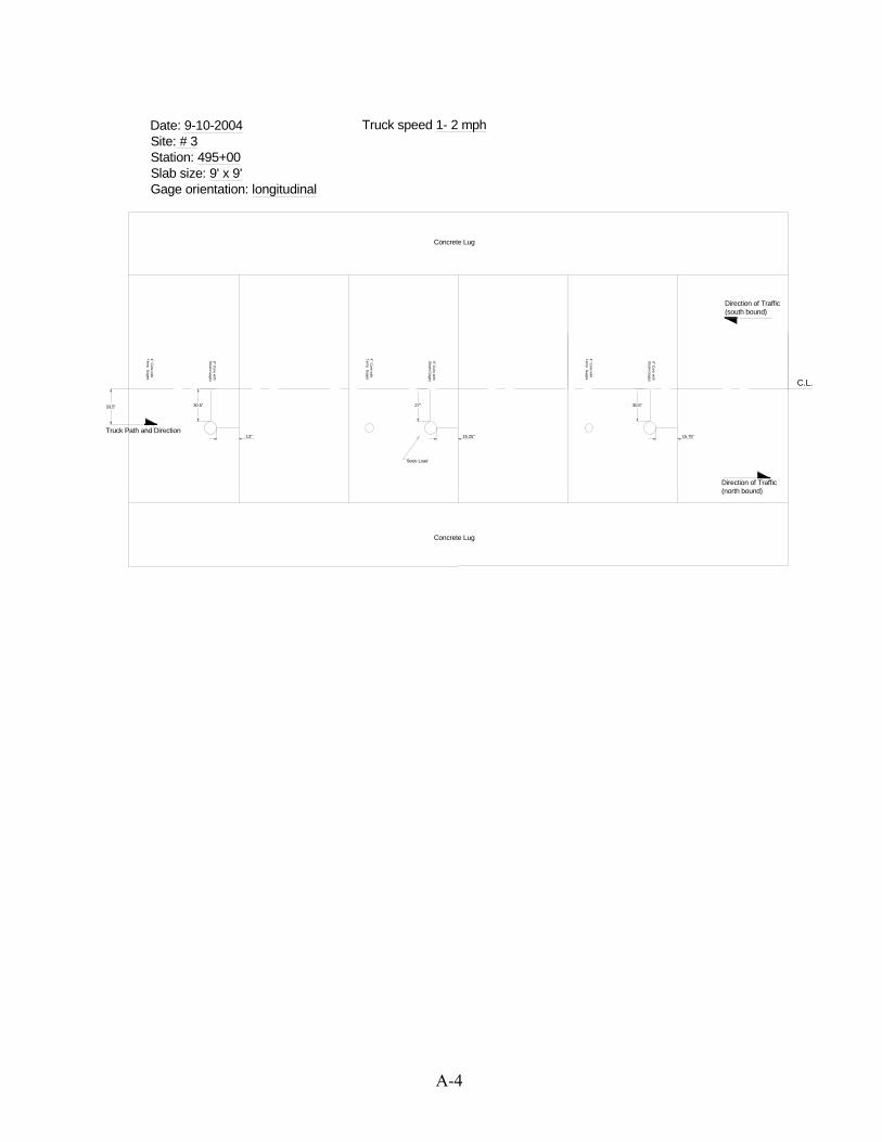
Date: 9-10-2004 Truck speed 1- 2 mph Site: # 3 Station: 495+00 Slab size: 9' x 9' Gage orientation: longitudinal

Static Load

13" Truck Path and Direction

Concrete Lug

4" Core w

ith Tem

p. Gages

6" Core w

ith S

train Gages

Concrete Lug

30.5" 33.5"

6" Core w

ith S

train Gages

4" Core w

ith Tem

p. Gages

27"

16.25" 15.75"

30.5"

4" Core w

ith Tem

p. Gages

6" Core w

ith S

train Gages C.L.

Direction of Traffic (south bound)

Direction of Traffic (north bound)

A-4

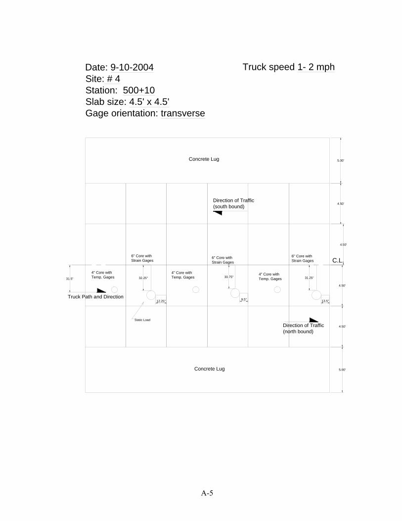
Date: 9-10-2004 Truck speed 1- 2 mph Site: # 4 Station: 500+10 Slab size: 4.5' x 4.5' Gage orientation: transverse

5.00'

4.50'

4.50'

4.50

4.50'

5.00'

Static Load

Direction of Traffic (north bound)

Direction of Traffic (south bound)

Concrete Lug

C.L.

Concrete Lug

6" Core with Strain Gages

4" Core with Temp. Gages

6" Core with Strain Gages

4" Core with Temp. Gages

6" Core with Strain Gages

4" Core with Temp. Gages

Truck Path and Direction

31.5" 32.25"

12.25"

30.75"

9.5"

31.25"

13.5"

'

A-5

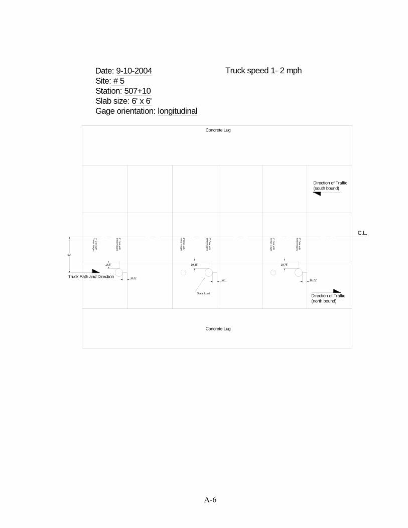
Date: 9-10-2004 Truck speed 1- 2 mph Site: # 5 Station: 507+10 Slab size: 6' x 6' Gage orientation: longitudinal

Static Load

60"

14.75"

19.75"

13"

19.25"

11.5"

16.5"

Direction of Traffic (north bound)

Direction of Traffic (south bound)

Truck Path and Direction

Concrete Lug

6" Core w

ith S

train Gages

4" Core w

ith Tem

p. Gages

6" Core w

ith S

train Gages

4" Core w

ith Tem

p. Gages

4" Core w

ith Tem

p. Gages

6" Core w

ith S

train Gages

Concrete Lug

C.L.

A-6

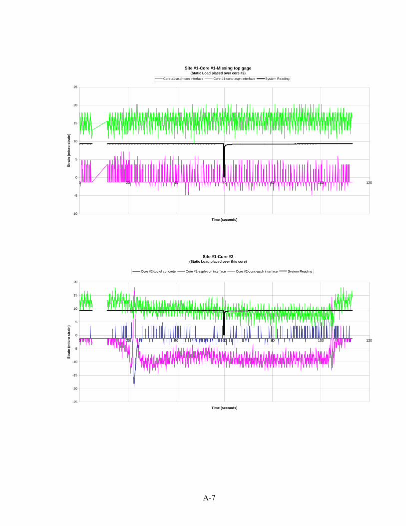
25

Site #1-Core #1-Missing top gage (Static Load placed over core #2)

Core #1-asph-con interface Core #1-conc-asph interface System Reading

20

15

10

5

0 0 20 40 60 80 100 120

-5

-10

Time (seconds)

Stra

in (m

icro

str

ain)

St

rain

(mic

ro s

trai

n)

Site #1-Core #2 (Static Load placed over this core)

Core #2-top of concrete Core #2-asph-con interface Core #2-conc-asph interface System Reading

20

15

10

5

0

0 20 40 60 80 100 120

-5

-10

-15

-20

-25

Time (seconds)

A-7

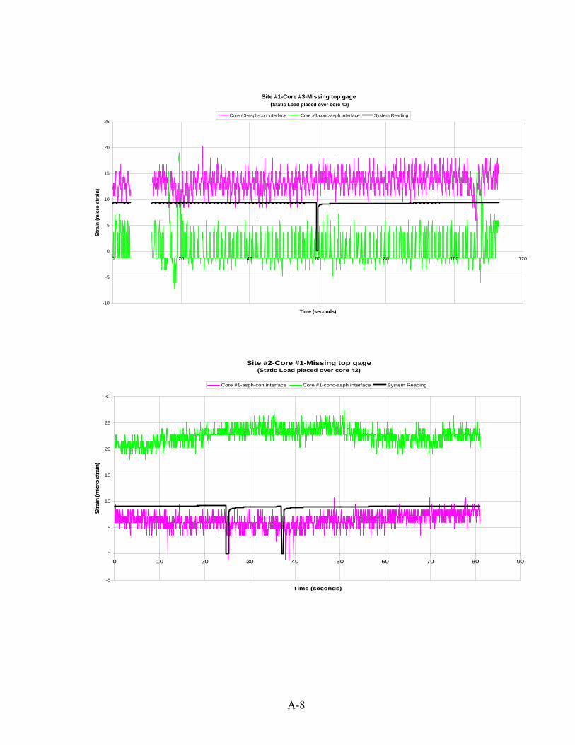
Stra

in (m

icro

str

ain)

St

rain

(mic

ro s

trai

n)

Site #1-Core #3-Missing top gage (Static Load placed over core #2)

Core #3-asph-con interface Core #3-conc-asph interface System Reading25

20

15

10

5

0 0 20 40 60 80 100 120

-5

-10

Time (seconds)

Site #2-Core #1-Missing top gage (Static Load placed over core #2)

Core #1-asph-con interface Core #1-conc-asph interface System Reading

30

25

20

15

10

5

0

0 10 20 30 40 50 60 70 80 90

-5

Time (seconds)

A-8

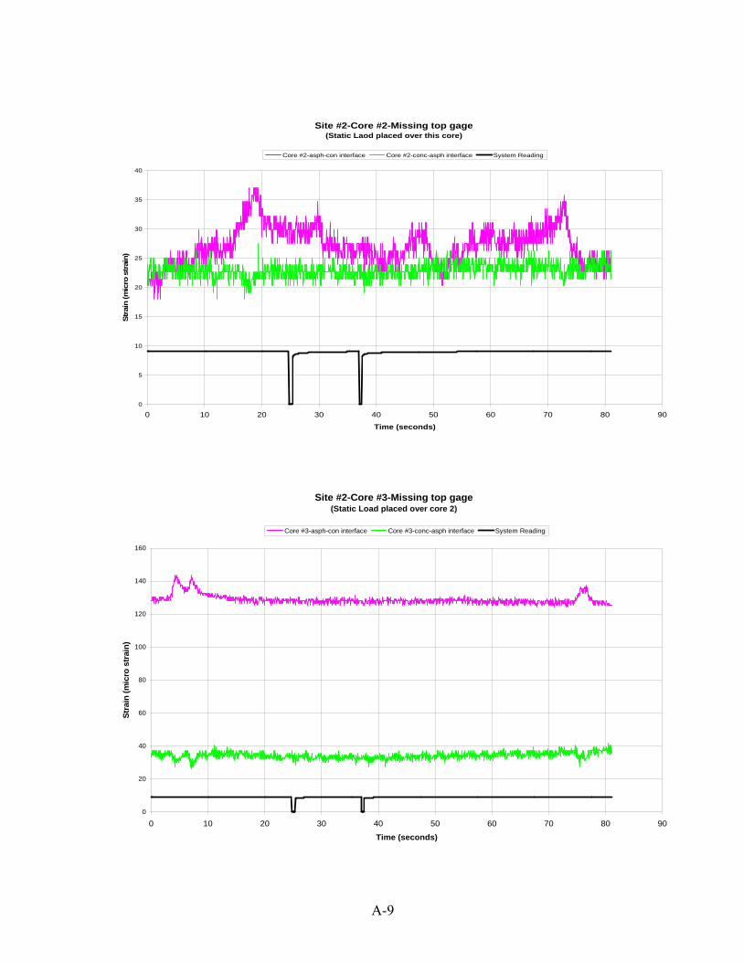
Stra

in (m

icro

str

ain)

St

rain

(mic

ro s

trai

n)

40

Site #2-Core #2-Missing top gage (Static Laod placed over this core)

Core #2-asph-con interface Core #2-conc-asph interface System Reading

35

30

25

20

15

10

5

0

0 10 20 30 40 50 60

Time (seconds)

70 80 90

160

Site #2-Core #3-Missing top gage (Static Load placed over core 2)

Core #3-asph-con interface Core #3-conc-asph interface System Reading

140

120

100

80

60

40

20

0

0 10 20 30 40 50 60 70 80

Time (seconds) 90

A-9

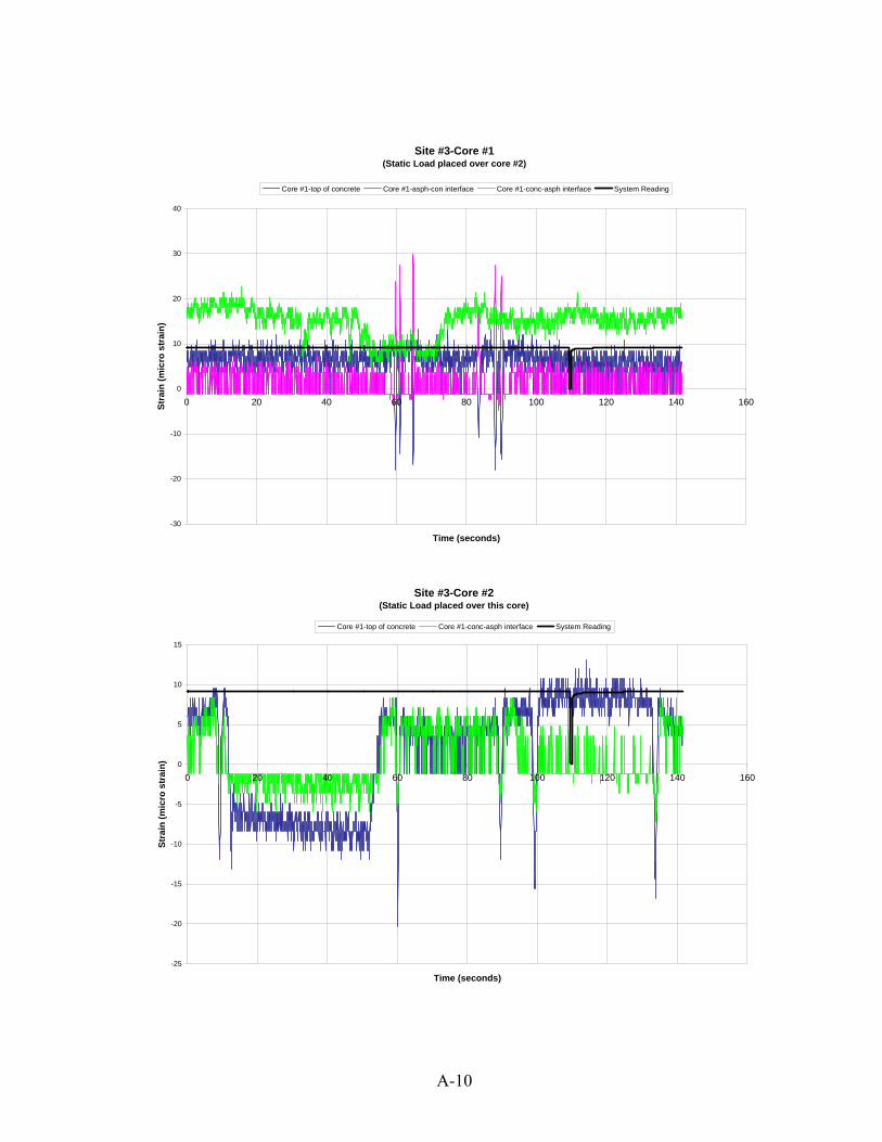
Stra

in (m

icro

str

ain)

St

rain

(mic

ro s

trai

n)

Site #3-Core #1 (Static Load placed over core #2)

Core #1-top of concrete Core #1-asph-con interface Core #1-conc-asph interface System Reading

40

30

20

10

0

0 20 40 60 80 100 120 140 160

-10

-20

-30

Time (seconds)

Site #3-Core #2 (Static Load placed over this core)

Core #1-top of concrete Core #1-conc-asph interface System Reading

15

10

5

0

0 20 40 60 80 100 120 140 160

-5

-10

-15

-20

-25

Time (seconds)

A-10

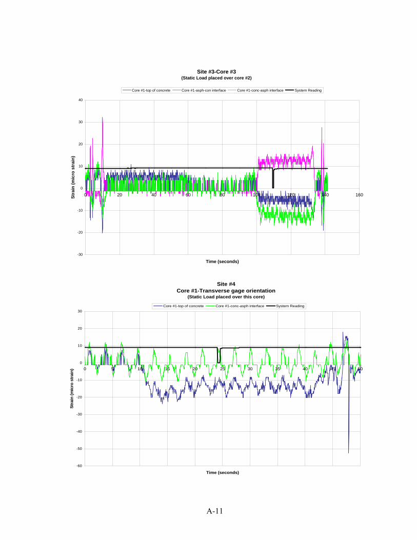
40

Stra

in (m

icro

str

ain)

St

rain

(mic

ro s

trai

n)

Site #3-Core #3 (Static Load placed over core #2)

Core #1-top of concrete Core #1-asph-con interface Core #1-conc-asph interface System Reading

30

20

10

0

0 20 40 60 80 100 120 140 160

-10

-20

-30

Time (seconds)

Site #4Core #1-Transverse gage orientation

(Static Load placed over this core)

Core #1-top of concrete Core #1-conc-asph interface System Reading30

20

10

0

0 5 10 15 20 25 30 35 40 45 50

-10

-20

-30

Time (seconds)

A-11

-60

-50

-40

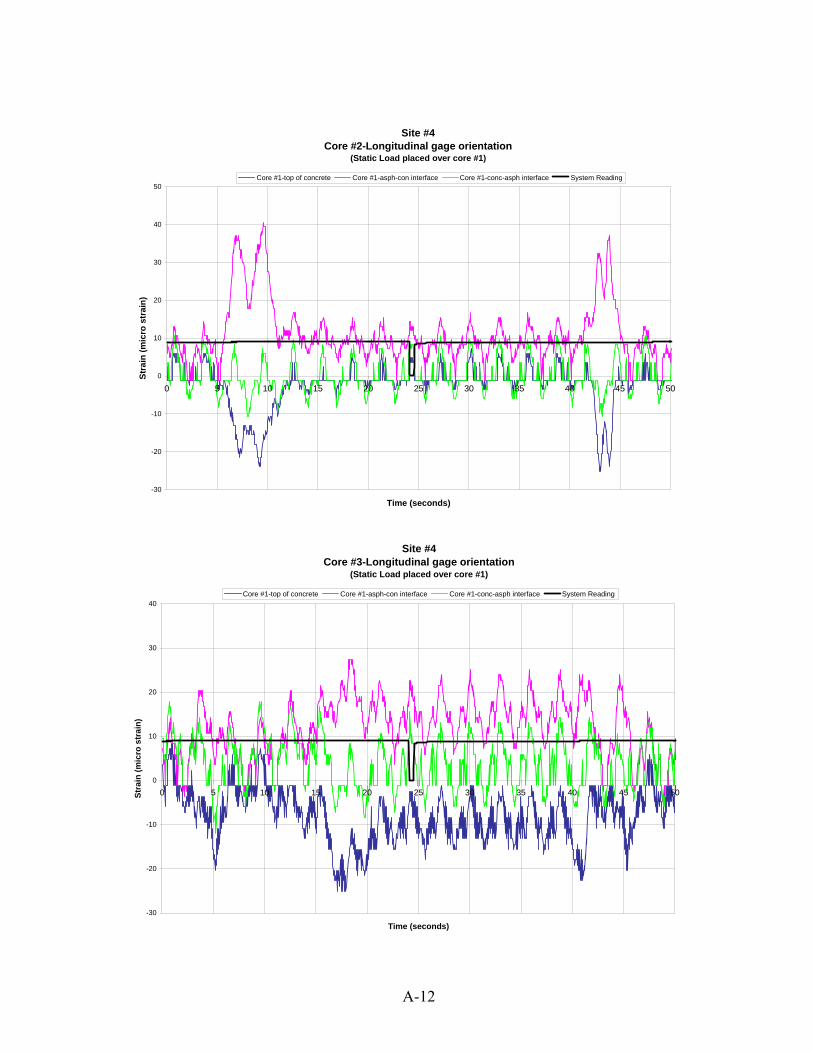
Stra

in (m

icro

str

ain)

St

rain

(mic

ro s

trai

n)

50

40

30

20

10

0

0

-10

-20

-30

40

30

20

10

0

0

-10

-20

-30

Site #4Core #2-Longitudinal gage orientation

(Static Load placed over core #1)

Core #1-top of concrete Core #1-asph-con interface Core #1-conc-asph interface System Reading

5 10 15 20 25 30 35 40 45 50

Time (seconds)

Site #4Core #3-Longitudinal gage orientation

(Static Load placed over core #1)

Core #1-top of concrete Core #1-asph-con interface Core #1-conc-asph interface System Reading

5 10 15 20 25 30 35 40 45 50

Time (seconds)

A-12

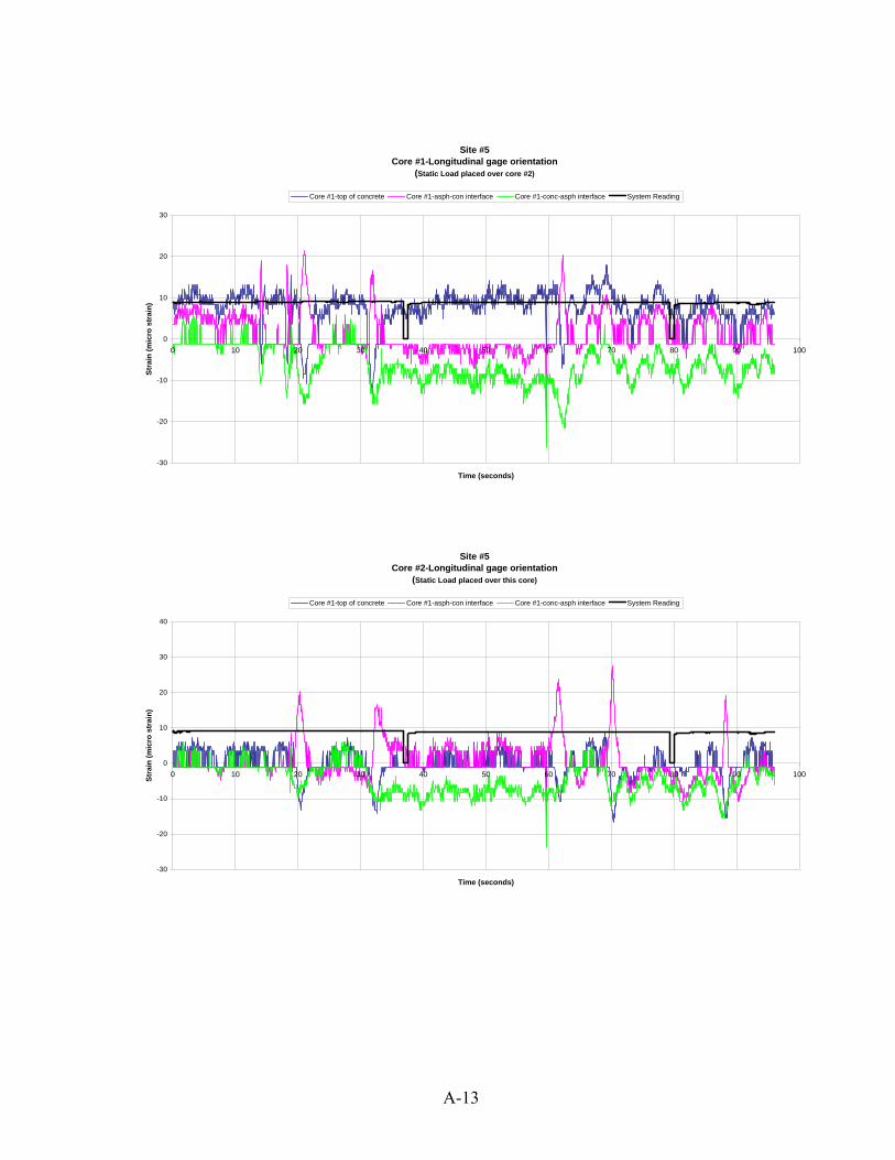
Stra

in (m

icro

str

ain)

St

rain

(mic

ro s

trai

n)

30

Core #1-top of concrete

Site #5 Core #1-Longitudinal gage orientation

(Static Load placed over core #2)

Core #1-asph-con interface Core #1-conc-asph interface System Reading

20

10

0 0 10 20 30 40 50 60 70 80 90 100

-10

-20

-30

Time (seconds)

40

Core #1-top of concrete

Site #5 Core #2-Longitudinal gage orientation

(Static Load placed over this core)

Core #1-asph-con interface Core #1-conc-asph interface System Reading

30

20

10

-10

0 0 10 20 30 40 50 60 70 80 90 100

-20

-30

Time (seconds)

A-13

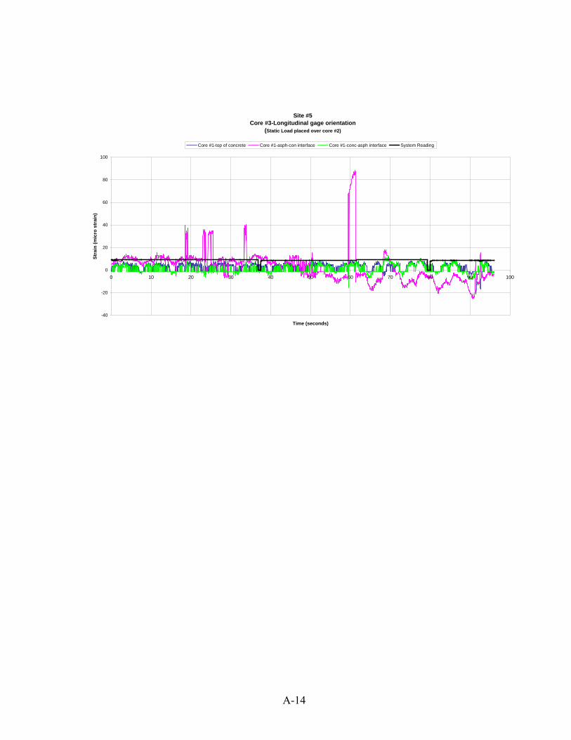
100

Stra

in (m

icro

str

ain)

Site #5Core #3-Longitudinal gage orientation

(Static Load placed over core #2)

Core #1-top of concrete Core #1-asph-con interface Core #1-conc-asph interface System Reading

80

60

40

20

0 0 10 20 30 40 50 60 70 80 90 100

-20

-40

Time (seconds)

A-14

APPENDIX B: IOWA 175 DESIGN EXAMPLE

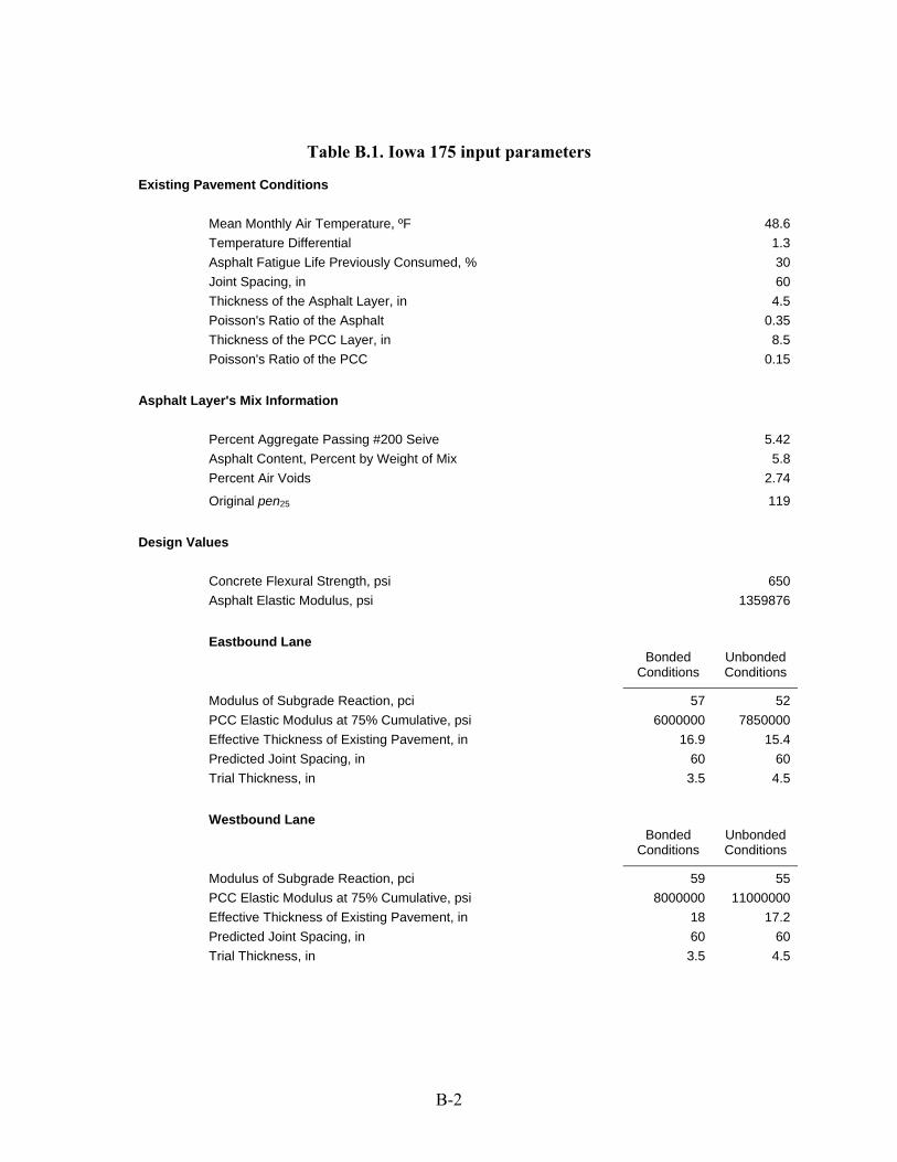
Table B.1. Iowa 175 input parameters

Existing Pavement Conditions

Mean Monthly Air Temperature, ºF Temperature Differential

Asphalt Fatigue Life Previously Consumed, % Joint Spacing, in

Thickness of the Asphalt Layer, in Poisson's Ratio of the Asphalt Thickness of the PCC Layer, in Poisson's Ratio of the PCC

48.6 1.3 30 60

4.5 0.35 8.5

0.15

Asphalt Layer's Mix Information

Percent Aggregate Passing #200 Seive Asphalt Content, Percent by Weight of Mix

Percent Air Voids

5.42 5.8

2.74

Original pen25 119

Design Values

Concrete Flexural Strength, psi Asphalt Elastic Modulus, psi

650 1359876

Eastbound Lane Bonded

Conditions Unbonded Conditions

Modulus of Subgrade Reaction, pci PCC Elastic Modulus at 75% Cumulative, psi Effective Thickness of Existing Pavement, in Predicted Joint Spacing, in

Trial Thickness, in

57 6000000

16.9 60 3.5

52 7850000

15.4 60 4.5

Westbound Lane Bonded

Conditions Unbonded Conditions

Modulus of Subgrade Reaction, pci PCC Elastic Modulus at 75% Cumulative, psi Effective Thickness of Existing Pavement, in Predicted Joint Spacing, in

Trial Thickness, in

59 8000000

18 60 3.5

55 11000000

17.2 60 4.5

B-2

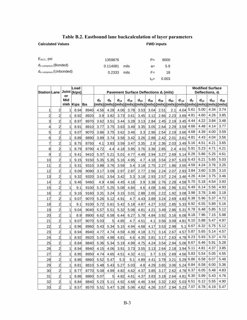
1 2 3 4 5 6 7 8 9

10 11 12 13 14 15 16 17 18 19 20 21 22 23 24 25 26 27 28 29 30 31 32 33

Table B.2. Eastbound lane backcalculation of layer parameters Calculated Values FWD inputs

EACC, psi 1359876 P= 9000 do compress (Bonded) 0.114081 mils a= 5.9 do compress (Unbonded) 0.2333 mils F= 18

tw= 0.003

Station Lane Joint or

Mid slab

Load (kips) Pavement Surface Deflections di (mils)

Modified Surface Deflections, di

Kips lbs d0

(mils) d8

(mils) d12

(mils) d18

(mils) d24

(mils) d36

(mils) d48

(mils) d60

(mils) d-12

(mils) d0

(mils) d12

(mils) d24

(mils) d36

(mils) 2 1 8.94 8940 4.56 4.28 4.06 3.78 3.53 3.04 2.51 2.1 4.04 5.61 5.00 4.34 3.74

2 1 8.92 8920 3.9 3.82 3.73 3.61 3.45 3.12 2.66 2.23 3.69 4.81 4.60 4.26 3.85

2 1 8.97 8970 3.62 3.51 3.44 3.28 3.13 2.84 2.45 2.19 3.45 4.44 4.22 3.84 3.48

2 1 8.91 8910 3.77 3.75 3.63 3.49 3.35 3.05 2.64 2.29 3.59 4.66 4.48 4.14 3.77

2 1 9.07 9070 3.86 3.75 3.62 3.46 3.3 2.96 2.54 2.19 3.66 4.68 4.39 4.00 3.59

2 1 8.89 8890 3.89 3.74 3.58 3.42 3.26 2.88 2.42 2.01 3.61 4.81 4.43 4.04 3.56

2 1 8.75 8750 4.1 3.83 3.59 3.47 3.35 2.9 2.36 2.03 3.49 5.16 4.51 4.21 3.65

2 1 8.79 8790 4.72 4.4 4.18 3.95 3.76 3.36 2.85 2.4 4.01 5.91 5.23 4.71 4.21

2 1 9.41 9410 5.37 5.21 5.01 4.77 4.49 3.94 3.27 2.69 5.14 6.28 5.86 5.25 4.61

2 1 9.15 9150 5.35 5.35 5.16 4.95 4.7 4.18 3.54 2.97 5.03 6.43 6.21 5.65 5.03

2 1 9.31 9310 3.88 3.76 3.59 3.4 3.18 2.75 2.27 1.86 3.55 4.59 4.24 3.76 3.25

2 1 9.09 9090 3.17 3.09 2.97 2.87 2.77 2.56 2.24 2.07 2.93 3.84 3.60 3.35 3.10

2 1 9.32 9320 3.61 3.54 3.42 3.3 3.18 2.93 2.57 2.24 3.46 4.26 4.04 3.75 3.46

2 1 9.46 9460 4.9 4.66 4.45 4.18 3.9 3.38 2.76 2.28 4.58 5.70 5.18 4.54 3.93

2 1 9.1 9100 5.37 5.25 5.08 4.84 4.6 4.08 3.46 2.96 5.01 6.49 6.14 5.56 4.93

2 1 9.16 9160 3.31 3.24 3.15 3.01 2.88 2.65 2.22 1.92 3.08 3.98 3.78 3.46 3.18

2 1 9.07 9070 5.26 5.12 4.91 4.7 4.43 3.89 3.24 2.69 4.83 6.38 5.96 5.37 4.72

2 1 9.1 9100 5.72 5.61 5.42 5.18 4.87 4.27 3.52 2.85 5.33 6.92 6.55 5.89 5.16

2 1 9.04 9040 5.57 5.51 5.32 5.08 4.81 4.21 3.49 2.86 5.31 6.78 6.48 5.85 5.12

2 1 8.9 8900 6.62 6.58 6.44 6.27 5.78 4.84 3.92 3.16 6.08 8.18 7.96 7.15 5.98

2 1 9.07 9070 5.03 5 4.85 4.7 4.51 4.1 3.56 3.09 4.81 6.10 5.88 5.47 4.97

2 1 8.96 8960 5.43 5.34 5.15 4.94 4.68 4.17 3.53 2.98 5.1 6.67 6.32 5.75 5.12

2 1 8.94 8940 4.77 4.74 4.59 4.39 4.18 3.71 3.14 2.67 4.57 5.87 5.65 5.14 4.57

2 1 8.92 8920 5.05 4.98 4.81 4.6 4.35 3.81 3.17 2.63 4.78 6.23 5.93 5.37 4.70

2 1 8.84 8840 5.36 5.34 5.19 4.99 4.75 4.24 3.54 2.94 5.06 6.67 6.46 5.91 5.28

2 1 8.94 8940 4.15 4.06 3.91 3.73 3.55 3.13 2.64 2.18 3.94 5.11 4.81 4.37 3.85

2 1 8.95 8950 4.74 4.65 4.51 4.32 4.11 3.7 3.15 2.69 4.56 5.83 5.54 5.05 4.55

2 1 8.86 8860 5.52 5.47 5.3 5.1 4.89 4.41 3.78 3.21 5.29 6.86 6.58 6.07 5.48

2 1 8.81 8810 5.48 5.43 5.27 5.03 4.8 4.29 3.65 3.06 5.24 6.84 6.58 6.00 5.36

2 1 8.77 8770 5.08 4.99 4.82 4.62 4.37 3.85 3.17 2.62 4.78 6.37 6.05 5.48 4.83

2 1 8.86 8860 5.07 5 4.82 4.61 4.37 3.83 3.18 2.64 4.81 6.30 5.99 5.43 4.76

2 1 8.84 8840 5.23 5.11 4.92 4.68 4.46 3.94 3.32 2.82 5.03 6.51 6.12 5.55 4.90

2 1 8.57 8570 5.51 5.47 5.28 5.06 4.82 4.26 3.57 2.94 5.23 7.07 6.78 6.19 5.47

B-3

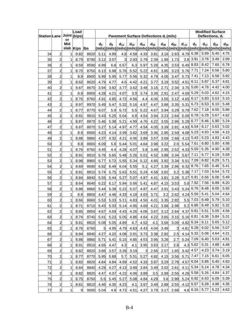
Station Lane Joint Load (kips) Pavement Surface Deflections di (mils)

Modified Surface Deflections, di

or Mid slab Kips lbs

d0 (mils)

d8 (mils)

d12 (mils)

d18 (mils)

d24 (mils)

d36 (mils)

d48 (mils)

d60 (mils)

d-12 (mils)

d0 (mils)

d12 (mils)

d24 (mils)

d36 (mils)

34 2 1 8.82 8820 5.11 4.99 4.8 4.58 4.33 3.81 3.16 2.63 4.79 6.38 5.99 5.40 4.75

35 2 1 8.79 8790 3.12 3.07 3 2.93 2.79 2.39 1.99 1.73 2.8 3.91 3.76 3.49 2.99

36 2 1 8.59 8590 6.89 6.8 6.57 6.3 5.97 5.28 4.35 3.53 6.49 8.83 8.42 7.65 6.76

37 2 1 8.75 8750 6.13 5.98 5.76 5.52 5.22 4.61 3.85 3.23 5.76 7.71 7.24 6.56 5.80

38 2 1 8.9 8900 5.99 5.95 5.77 5.56 5.32 4.79 4.06 3.47 5.73 7.41 7.13 6.58 5.92

39 2 1 8.62 8620 4.79 4.77 4.6 4.42 4.21 3.77 3.19 3.52 4.51 6.11 5.87 5.37 4.81

40 2 1 8.67 8670 3.94 3.92 3.77 3.62 3.48 3.15 2.71 2.34 3.75 5.00 4.78 4.42 4.00

41 2 1 8.9 8900 4.28 4.21 4.07 3.9 3.74 3.36 2.91 2.47 4.09 5.29 5.03 4.62 4.15

42 2 1 8.76 8760 4.91 4.85 4.72 4.56 4.4 4.06 3.55 3.12 4.65 6.17 5.93 5.53 5.10

43 2 1 8.97 8970 5.49 5.47 5.32 5.16 4.97 4.47 3.86 3.35 5.31 6.73 6.53 6.10 5.48

44 2 1 8.77 8770 6.07 5.9 5.72 5.5 5.22 4.67 3.94 3.29 5.79 7.62 7.18 6.55 5.86

45 2 1 8.81 8810 5.43 5.25 5.04 4.8 4.54 3.94 3.23 2.64 5.09 6.78 6.29 5.67 4.92

46 2 1 8.87 8870 5.46 5.38 5.21 4.99 4.76 4.22 3.55 2.96 5.28 6.77 6.46 5.90 5.24

47 2 1 8.87 8870 5.27 5.14 4.97 4.77 4.54 4.05 3.39 2.81 4.93 6.54 6.17 5.63 5.02

48 2 1 8.9 8900 4.23 4.14 3.99 3.82 3.69 3.36 2.95 2.59 4.08 5.23 4.93 4.56 4.15

49 2 1 8.86 8860 4.37 4.32 4.21 4.06 3.89 3.57 3.09 2.69 4.13 5.43 5.23 4.83 4.43

50 2 1 8.8 8800 6.09 5.8 5.44 5.01 4.64 3.98 3.22 2.9 5.54 7.61 6.80 5.80 4.98

51 2 1 8.76 8760 4.45 4.4 4.26 4.07 3.9 3.49 2.95 2.52 4.33 5.59 5.35 4.90 4.38

52 2 1 8.91 8910 5.76 5.65 5.48 5.26 5.01 4.52 3.88 3.34 5.67 7.11 6.77 6.19 5.58

53 2 1 8.96 8960 5.77 5.72 5.55 5.34 5.12 4.65 3.92 3.34 5.51 7.09 6.82 6.29 5.71

54 2 1 8.69 8690 6.92 6.49 6.04 5.55 5.1 4.27 3.39 2.96 6.32 8.76 7.65 6.46 5.41

55 2 1 8.81 8810 5.74 5.75 5.63 5.51 5.24 4.58 3.82 3.2 5.36 7.17 7.03 6.54 5.72

56 2 1 8.84 8840 5.55 5.44 5.27 5.07 4.87 4.41 3.81 3.28 5.27 6.91 6.56 6.06 5.49

57 2 1 8.64 8640 6.22 6.17 5.94 5.66 5.41 4.87 4.15 3.53 5.8 7.92 7.56 6.89 6.20

58 2 1 8.86 8860 5.44 5.38 5.22 5.07 4.87 4.47 3.91 3.43 5.24 6.76 6.48 6.05 5.55

59 2 1 8.8 8800 4.47 4.46 4.33 4.18 4.03 3.71 3.2 2.62 4.24 5.59 5.41 5.04 4.64

60 2 1 8.66 8660 5.53 5.33 5.11 4.83 4.56 4.01 3.35 2.82 5.5 7.03 6.49 5.79 5.10

61 2 1 8.71 8710 5.43 5.33 5.14 4.95 4.69 4.21 3.56 2.98 5.2 6.86 6.49 5.92 5.32

62 2 1 8.85 8850 4.67 4.59 4.43 4.26 4.06 3.67 3.12 2.64 4.37 5.81 5.51 5.05 4.56

63 2 1 8.74 8740 5.41 5.23 5.05 4.86 4.64 4.22 3.65 3.15 5.16 6.81 6.36 5.84 5.31

64 2 1 8.81 8810 5.08 5.05 4.89 4.7 4.52 4.1 3.56 3.09 4.82 6.34 6.11 5.65 5.12

65 2 1 8.76 8760 5 4.95 4.79 4.63 4.43 4.04 3.49 3 4.81 6.28 6.02 5.56 5.07

66 2 1 8.84 8840 4.27 4.22 4.08 3.91 3.73 3.38 2.92 2.5 4.14 5.32 5.08 4.64 4.21

67 2 1 8.86 8860 5.71 5.41 5.15 4.85 4.53 3.95 3.26 2.7 5.24 7.09 6.40 5.63 4.91

68 2 1 8.91 8910 4.55 4.47 4.3 4.1 3.95 3.63 3.17 2.8 4.3 5.62 5.31 4.88 4.48

69 2 1 8.82 8820 3.66 3.57 3.39 3.19 3 2.56 2.07 1.65 3.42 4.57 4.23 3.74 3.19

70 2 1 8.77 8770 5.95 5.88 5.7 5.51 5.27 4.82 4.15 3.56 5.71 7.47 7.15 6.61 6.05

71 2 1 8.82 8820 4.84 4.84 4.69 4.52 4.33 3.87 3.29 2.76 4.57 6.04 5.85 5.40 4.83

72 2 1 8.84 8840 4.29 4.27 4.13 3.99 3.84 3.49 3.02 2.61 4.11 5.34 5.14 4.78 4.34

74 2 1 8.82 8820 4.47 4.37 4.22 4.06 3.88 3.5 2.99 2.56 4.26 5.58 5.26 4.84 4.37

75 2 1 8.75 8750 5.5 5.45 5.27 5.08 4.84 4.29 3.6 2.99 5.24 6.92 6.63 6.09 5.39

76 2 1 8.81 8810 4.46 4.35 4.23 4.1 3.97 3.48 2.88 2.55 4.12 5.57 5.28 4.96 4.35

77 2 1 9 9000 5.04 4.9 4.72 4.51 4.27 3.79 3.17 2.68 4.8 6.16 5.77 5.22 4.63

B-4

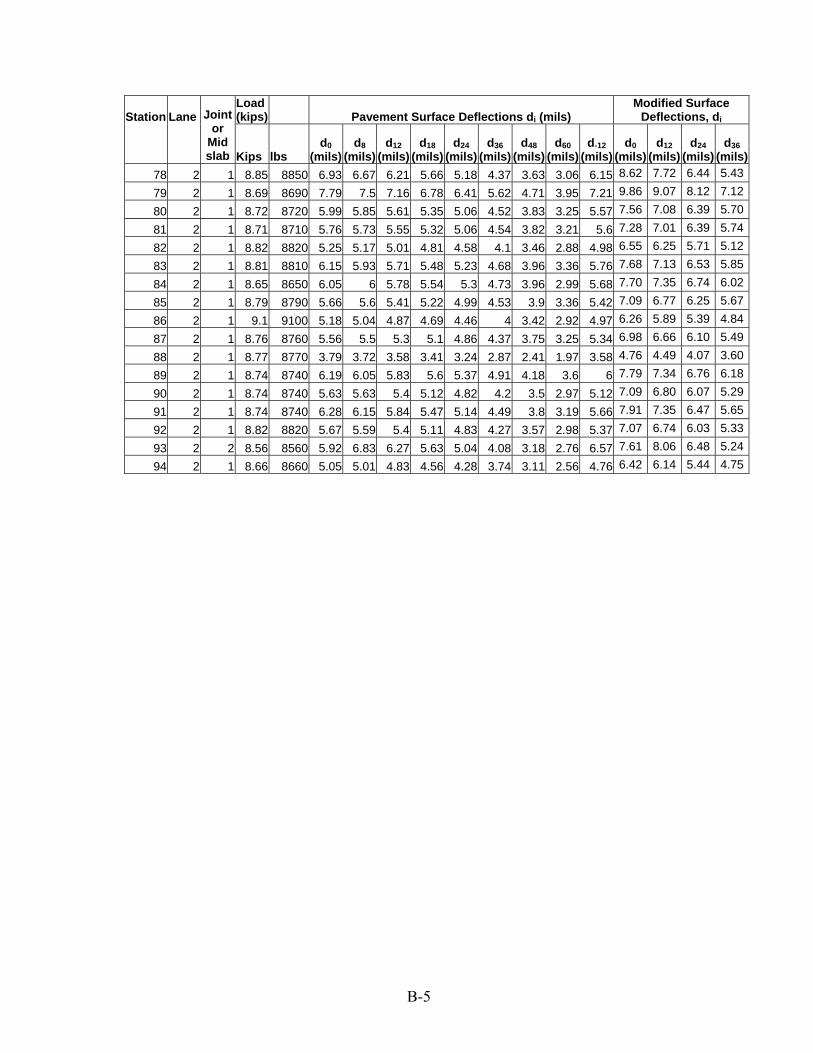
Station Lane Joint Load (kips) Pavement Surface Deflections di (mils)

Modified Surface Deflections, di

or Mid slab Kips lbs

d0 (mils)

d8 (mils)

d12 (mils)

d18 (mils)

d24 (mils)

d36 (mils)

d48 (mils)

d60 (mils)

d-12 (mils)

d0 (mils)

d12 (mils)

d24 (mils)

d36 (mils)

78 2 1 8.85 8850 6.93 6.67 6.21 5.66 5.18 4.37 3.63 3.06 6.15 8.62 7.72 6.44 5.43

79 2 1 8.69 8690 7.79 7.5 7.16 6.78 6.41 5.62 4.71 3.95 7.21 9.86 9.07 8.12 7.12

80 2 1 8.72 8720 5.99 5.85 5.61 5.35 5.06 4.52 3.83 3.25 5.57 7.56 7.08 6.39 5.70

81 2 1 8.71 8710 5.76 5.73 5.55 5.32 5.06 4.54 3.82 3.21 5.6 7.28 7.01 6.39 5.74

82 2 1 8.82 8820 5.25 5.17 5.01 4.81 4.58 4.1 3.46 2.88 4.98 6.55 6.25 5.71 5.12

83 2 1 8.81 8810 6.15 5.93 5.71 5.48 5.23 4.68 3.96 3.36 5.76 7.68 7.13 6.53 5.85

84 2 1 8.65 8650 6.05 6 5.78 5.54 5.3 4.73 3.96 2.99 5.68 7.70 7.35 6.74 6.02

85 2 1 8.79 8790 5.66 5.6 5.41 5.22 4.99 4.53 3.9 3.36 5.42 7.09 6.77 6.25 5.67

86 2 1 9.1 9100 5.18 5.04 4.87 4.69 4.46 4 3.42 2.92 4.97 6.26 5.89 5.39 4.84

87 2 1 8.76 8760 5.56 5.5 5.3 5.1 4.86 4.37 3.75 3.25 5.34 6.98 6.66 6.10 5.49

88 2 1 8.77 8770 3.79 3.72 3.58 3.41 3.24 2.87 2.41 1.97 3.58 4.76 4.49 4.07 3.60

89 2 1 8.74 8740 6.19 6.05 5.83 5.6 5.37 4.91 4.18 3.6 6 7.79 7.34 6.76 6.18

90 2 1 8.74 8740 5.63 5.63 5.4 5.12 4.82 4.2 3.5 2.97 5.12 7.09 6.80 6.07 5.29

91 2 1 8.74 8740 6.28 6.15 5.84 5.47 5.14 4.49 3.8 3.19 5.66 7.91 7.35 6.47 5.65

92 2 1 8.82 8820 5.67 5.59 5.4 5.11 4.83 4.27 3.57 2.98 5.37 7.07 6.74 6.03 5.33

93 2 2 8.56 8560 5.92 6.83 6.27 5.63 5.04 4.08 3.18 2.76 6.57 7.61 8.06 6.48 5.24

94 2 1 8.66 8660 5.05 5.01 4.83 4.56 4.28 3.74 3.11 2.56 4.76 6.42 6.14 5.44 4.75

B-5

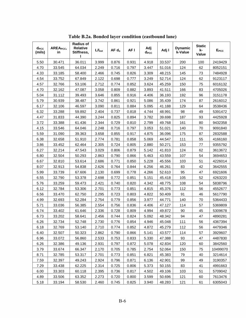
Table B.2a. Bonded layer condition (eastbound lane)

dPCC (mils)

AREAPCC, in

Radius of Relative

Stiffness, l

L/lest AF do AF l Adj dPCC

Adj l Dynamic k-Value

Static k-

Value EPCC

5.50 30.471 36.011 3.999 0.876 0.931 4.918 33.537 200 100 2419429 4.70 33.545 64.034 2.249 0.716 0.797 3.447 51.016 124 62 8052151 4.33 33.185 58.400 2.466 0.745 0.826 3.309 48.215 145 73 7484928 4.54 33.752 67.849 2.122 0.698 0.777 3.249 52.714 124 62 9123117 4.57 32.766 53.106 2.712 0.774 0.852 3.624 45.259 150 75 6016132 4.70 32.162 47.087 3.058 0.809 0.882 3.893 41.511 166 83 4705026 5.04 31.112 39.493 3.646 0.855 0.916 4.406 36.193 192 96 3151178 5.79 30.939 38.487 3.742 0.861 0.921 5.086 35.439 174 87 2616012 6.17 32.106 46.597 3.090 0.811 0.884 5.095 41.188 129 64 3538436 6.32 33.288 59.892 2.404 0.737 0.818 4.744 48.991 98 49 5391472 4.47 31.833 44.390 3.244 0.825 0.894 3.782 39.698 187 93 4425928 3.72 33.388 61.436 2.344 0.729 0.810 2.799 49.768 161 80 9432358 4.15 33.546 64.046 2.248 0.716 0.797 3.053 51.021 140 70 9091840 5.59 31.090 39.363 3.658 0.855 0.917 4.875 36.096 175 87 2832588 6.38 32.658 51.910 2.774 0.781 0.858 5.069 44.547 111 55 4166160 3.86 33.452 62.464 2.305 0.724 0.805 2.880 50.271 153 77 9355792 6.27 32.214 47.543 3.029 0.806 0.879 5.142 41.810 124 62 3613672 6.80 32.504 50.293 2.863 0.790 0.866 5.463 43.559 107 54 3694653 6.67 32.810 53.614 2.686 0.771 0.850 5.228 45.556 103 51 4226014 8.07 32.913 54.838 2.626 0.764 0.844 6.256 46.261 83 42 3642555 5.99 33.739 67.606 2.130 0.699 0.778 4.266 52.610 95 47 6921606 6.55 32.790 53.378 2.698 0.772 0.851 5.151 45.418 105 52 4263220 5.76 33.259 59.473 2.421 0.740 0.820 4.342 48.775 108 54 5838796 6.12 32.784 53.306 2.701 0.773 0.851 4.815 45.376 112 56 4552677 6.56 33.470 62.750 2.295 0.723 0.803 4.822 50.409 91 46 5617790 4.99 32.693 52.284 2.754 0.779 0.856 3.977 44.771 140 70 5364433 5.71 33.036 56.385 2.554 0.756 0.836 4.406 47.127 114 57 5369809 6.74 33.402 61.646 2.336 0.728 0.809 4.994 49.872 90 45 5309678 6.73 33.202 58.641 2.456 0.744 0.824 5.092 48.342 94 47 4890281 6.26 32.734 52.748 2.730 0.776 0.854 4.946 45.048 111 56 4367394 6.18 32.769 53.140 2.710 0.774 0.852 4.872 45.279 112 56 4479346 6.40 32.507 50.323 2.862 0.790 0.866 5.141 43.577 114 57 3929607 6.96 33.072 56.860 2.533 0.753 0.833 5.330 47.388 93 47 4487830 6.26 32.386 49.136 2.931 0.797 0.872 5.078 42.834 120 60 3842560 3.79 33.674 66.347 2.170 0.705 0.785 2.754 52.064 150 75 10499070 8.71 32.785 53.317 2.701 0.773 0.851 6.821 45.383 79 40 3214614 7.59 32.397 49.243 2.924 0.796 0.871 6.136 42.901 99 49 3190357 7.29 33.438 62.225 2.314 0.725 0.806 5.373 50.155 83 41 4991663 6.00 33.303 60.118 2.395 0.736 0.817 4.502 49.106 103 51 5709042 4.89 33.506 63.352 2.273 0.720 0.800 3.599 50.696 121 60 7613476 5.18 33.194 58.530 2.460 0.745 0.825 3.940 48.283 121 61 6305043

B-6

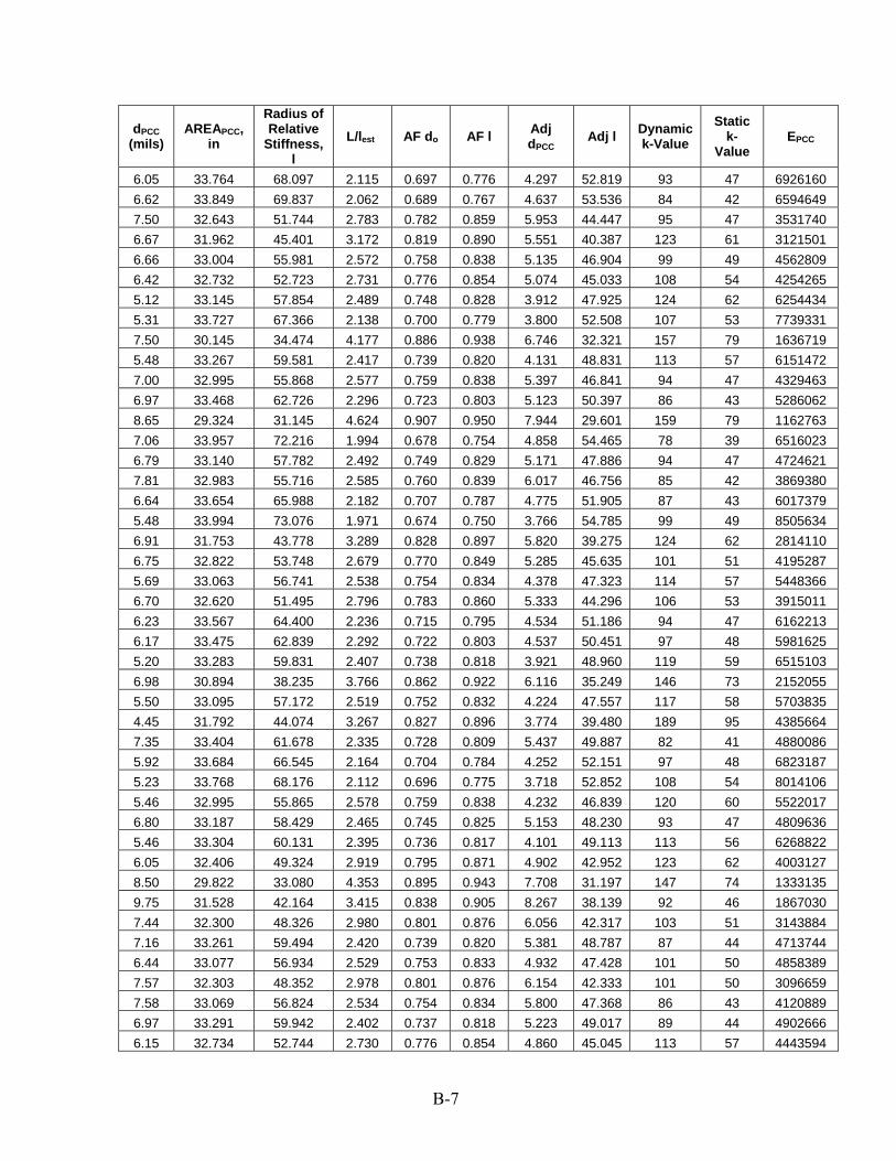
dPCC (mils)

AREAPCC, in

Radius of Relative

Stiffness, l

L/lest AF do AF l Adj dPCC

Adj l Dynamic k-Value

Static k-

Value EPCC

6.05 33.764 68.097 2.115 0.697 0.776 4.297 52.819 93 47 6926160 6.62 33.849 69.837 2.062 0.689 0.767 4.637 53.536 84 42 6594649 7.50 32.643 51.744 2.783 0.782 0.859 5.953 44.447 95 47 3531740 6.67 31.962 45.401 3.172 0.819 0.890 5.551 40.387 123 61 3121501 6.66 33.004 55.981 2.572 0.758 0.838 5.135 46.904 99 49 4562809 6.42 32.732 52.723 2.731 0.776 0.854 5.074 45.033 108 54 4254265 5.12 33.145 57.854 2.489 0.748 0.828 3.912 47.925 124 62 6254434 5.31 33.727 67.366 2.138 0.700 0.779 3.800 52.508 107 53 7739331 7.50 30.145 34.474 4.177 0.886 0.938 6.746 32.321 157 79 1636719 5.48 33.267 59.581 2.417 0.739 0.820 4.131 48.831 113 57 6151472 7.00 32.995 55.868 2.577 0.759 0.838 5.397 46.841 94 47 4329463 6.97 33.468 62.726 2.296 0.723 0.803 5.123 50.397 86 43 5286062 8.65 29.324 31.145 4.624 0.907 0.950 7.944 29.601 159 79 1162763 7.06 33.957 72.216 1.994 0.678 0.754 4.858 54.465 78 39 6516023 6.79 33.140 57.782 2.492 0.749 0.829 5.171 47.886 94 47 4724621 7.81 32.983 55.716 2.585 0.760 0.839 6.017 46.756 85 42 3869380 6.64 33.654 65.988 2.182 0.707 0.787 4.775 51.905 87 43 6017379 5.48 33.994 73.076 1.971 0.674 0.750 3.766 54.785 99 49 8505634 6.91 31.753 43.778 3.289 0.828 0.897 5.820 39.275 124 62 2814110 6.75 32.822 53.748 2.679 0.770 0.849 5.285 45.635 101 51 4195287 5.69 33.063 56.741 2.538 0.754 0.834 4.378 47.323 114 57 5448366 6.70 32.620 51.495 2.796 0.783 0.860 5.333 44.296 106 53 3915011 6.23 33.567 64.400 2.236 0.715 0.795 4.534 51.186 94 47 6162213 6.17 33.475 62.839 2.292 0.722 0.803 4.537 50.451 97 48 5981625 5.20 33.283 59.831 2.407 0.738 0.818 3.921 48.960 119 59 6515103 6.98 30.894 38.235 3.766 0.862 0.922 6.116 35.249 146 73 2152055 5.50 33.095 57.172 2.519 0.752 0.832 4.224 47.557 117 58 5703835 4.45 31.792 44.074 3.267 0.827 0.896 3.774 39.480 189 95 4385664 7.35 33.404 61.678 2.335 0.728 0.809 5.437 49.887 82 41 4880086 5.92 33.684 66.545 2.164 0.704 0.784 4.252 52.151 97 48 6823187 5.23 33.768 68.176 2.112 0.696 0.775 3.718 52.852 108 54 8014106 5.46 32.995 55.865 2.578 0.759 0.838 4.232 46.839 120 60 5522017 6.80 33.187 58.429 2.465 0.745 0.825 5.153 48.230 93 47 4809636 5.46 33.304 60.131 2.395 0.736 0.817 4.101 49.113 113 56 6268822 6.05 32.406 49.324 2.919 0.795 0.871 4.902 42.952 123 62 4003127 8.50 29.822 33.080 4.353 0.895 0.943 7.708 31.197 147 74 1333135 9.75 31.528 42.164 3.415 0.838 0.905 8.267 38.139 92 46 1867030 7.44 32.300 48.326 2.980 0.801 0.876 6.056 42.317 103 51 3143884 7.16 33.261 59.494 2.420 0.739 0.820 5.381 48.787 87 44 4713744 6.44 33.077 56.934 2.529 0.753 0.833 4.932 47.428 101 50 4858389 7.57 32.303 48.352 2.978 0.801 0.876 6.154 42.333 101 50 3096659 7.58 33.069 56.824 2.534 0.754 0.834 5.800 47.368 86 43 4120889 6.97 33.291 59.942 2.402 0.737 0.818 5.223 49.017 89 44 4902666 6.15 32.734 52.744 2.730 0.776 0.854 4.860 45.045 113 57 4443594

B-7

dPCC (mils)

AREAPCC, in

Radius of Relative

Stiffness, l

L/lest AF do AF l Adj dPCC

Adj l Dynamic k-Value

Static k-

Value EPCC

6.87 33.086 57.054 2.524 0.752 0.832 5.255 47.493 94 47 4572828 4.64 32.780 53.261 2.704 0.773 0.851 3.676 45.350 147 74 5955386 7.68 32.865 54.259 2.654 0.768 0.846 5.982 45.930 88 44 3754985 6.97 32.689 52.243 2.756 0.779 0.857 5.520 44.747 101 50 3860467 7.79 31.641 42.959 3.352 0.833 0.901 6.588 38.702 113 56 2413256 6.96 32.598 51.269 2.809 0.784 0.861 5.548 44.159 103 51 3740040 7.50 33.473 62.799 2.293 0.723 0.803 5.499 50.432 80 40 4931568 6.30 32.563 50.904 2.829 0.786 0.863 5.046 43.936 114 57 4070375

B-8

Table B.2b. Unbonded layer conditions (eastbound lane)

dPCC (mils) AREAPCC

Radius of Relative

Stiffness, l

L/lest AF do AF l Adj dPCC

Adj l Dynamic k-Value

Static k-

Value EPCC

5.38 31.013 38.914 3.701 0.858 0.919 4.817 35.760 180 90 2813376 4.58 34.263 80.097 1.798 0.644 0.713 3.097 57.115 111 55 11248235 4.21 33.955 72.167 1.995 0.678 0.754 3.010 54.446 125 63 10508922 4.42 34.500 87.778 1.641 0.613 0.673 2.856 59.089 112 56 13059783 4.45 33.483 62.975 2.287 0.722 0.802 3.380 50.516 129 65 8050875 4.58 32.843 54.000 2.667 0.769 0.848 3.703 45.780 144 72 6026551 4.92 31.720 43.535 3.308 0.830 0.898 4.278 39.106 170 85 3795032 5.68 31.463 41.725 3.451 0.841 0.907 4.968 37.824 156 78 3055295 6.05 32.620 51.503 2.796 0.783 0.860 4.917 44.301 115 58 4247685 6.20 33.812 69.075 2.085 0.692 0.771 4.453 53.226 89 44 6787767 4.35 32.541 50.674 2.842 0.788 0.864 3.612 43.794 161 80 5648996 3.60 34.294 81.027 1.777 0.640 0.708 2.455 57.386 138 69 14321613 4.03 34.361 83.089 1.733 0.632 0.697 2.692 57.954 124 62 13325605 5.47 31.637 42.934 3.354 0.833 0.901 4.750 38.684 156 78 3344036 6.26 33.166 58.141 2.477 0.747 0.827 4.848 48.078 100 50 5080116 3.74 34.327 82.008 1.756 0.636 0.703 2.528 57.662 133 67 14042762 6.15 32.722 52.612 2.737 0.777 0.855 4.957 44.967 111 56 4342197 6.68 32.976 55.627 2.589 0.760 0.840 5.257 46.706 97 49 4419280 6.55 33.298 60.054 2.398 0.737 0.817 4.994 49.074 93 46 5139586 7.95 33.316 60.325 2.387 0.735 0.816 6.017 49.211 77 38 4289664 5.87 34.303 81.277 1.772 0.639 0.707 3.898 57.457 87 43 9042863 6.44 33.286 59.870 2.405 0.738 0.818 4.918 48.980 95 47 5198580 5.64 33.836 69.561 2.070 0.690 0.768 4.050 53.425 97 48 7519089 6.00 33.316 60.320 2.387 0.735 0.816 4.580 49.209 101 50 5635127 6.44 33.978 72.707 1.981 0.675 0.752 4.507 54.649 83 42 7072427 4.87 33.345 60.767 2.370 0.733 0.814 3.744 49.434 122 61 6958010 5.59 33.612 65.206 2.208 0.711 0.791 4.141 51.554 101 51 6844708 6.62 33.895 70.829 2.033 0.684 0.761 4.689 53.931 82 41 6618811 6.61 33.692 66.695 2.159 0.703 0.783 4.814 52.217 85 43 6040969 6.14 33.253 59.389 2.425 0.740 0.821 4.717 48.732 100 50 5365404 6.06 33.295 60.008 2.400 0.737 0.817 4.639 49.050 100 50 5526921 6.28 33.010 56.055 2.569 0.758 0.837 4.933 46.945 103 51 4758261 6.84 33.544 64.000 2.250 0.717 0.797 5.069 51.000 85 42 5471036 6.14 32.898 54.660 2.634 0.765 0.844 4.879 46.160 107 54 4649947 3.67 34.572 90.493 1.591 0.603 0.659 2.356 59.647 133 67 16130848 8.59 33.156 58.004 2.483 0.747 0.828 6.596 48.005 73 37 3722472 7.48 32.818 53.707 2.681 0.771 0.849 5.941 45.610 90 45 3728175 7.17 33.894 70.803 2.034 0.684 0.762 5.066 53.920 76 38 6123574 5.88 33.856 69.994 2.057 0.688 0.766 4.206 53.599 92 46 7288421 4.77 34.194 78.138 1.843 0.652 0.723 3.259 56.516 107 54 10462283 5.06 33.835 69.540 2.071 0.690 0.768 3.651 53.416 107 54 8338560

B-9

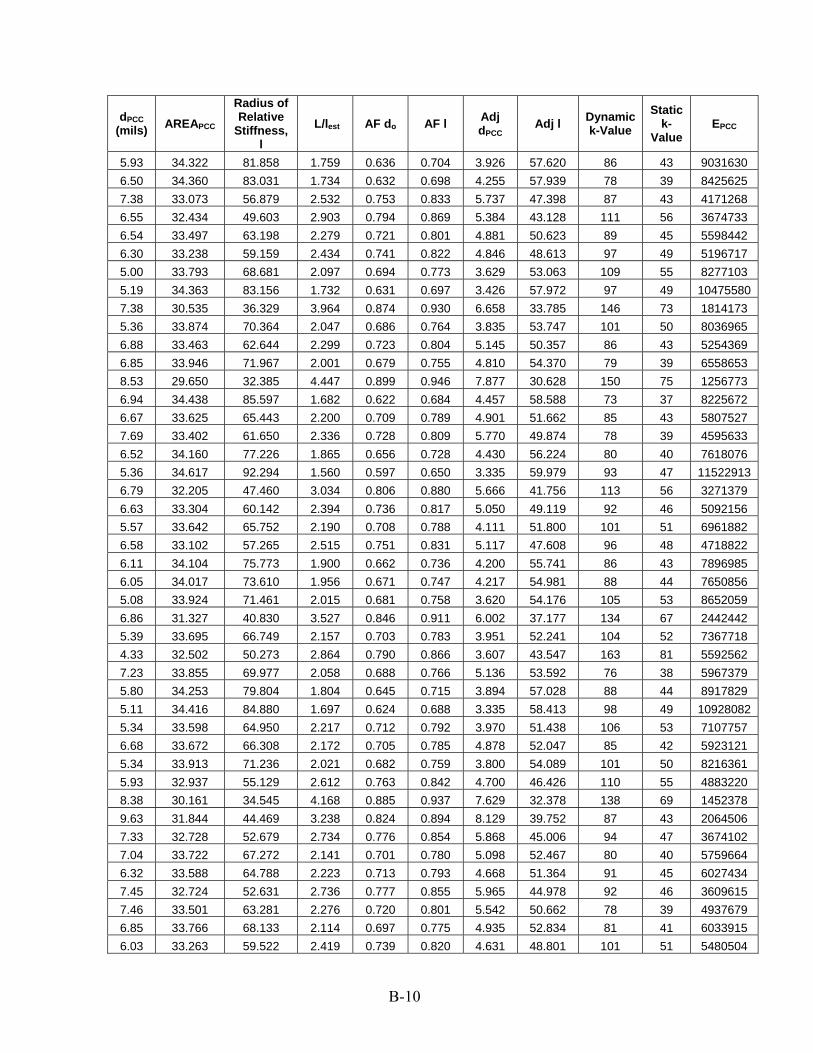
dPCC (mils) AREAPCC

Radius of Relative

Stiffness, l

L/lest AF do AF l Adj dPCC

Adj l Dynamic k-Value

Static k-

Value EPCC

5.93 34.322 81.858 1.759 0.636 0.704 3.926 57.620 86 43 9031630 6.50 34.360 83.031 1.734 0.632 0.698 4.255 57.939 78 39 8425625 7.38 33.073 56.879 2.532 0.753 0.833 5.737 47.398 87 43 4171268 6.55 32.434 49.603 2.903 0.794 0.869 5.384 43.128 111 56 3674733 6.54 33.497 63.198 2.279 0.721 0.801 4.881 50.623 89 45 5598442 6.30 33.238 59.159 2.434 0.741 0.822 4.846 48.613 97 49 5196717 5.00 33.793 68.681 2.097 0.694 0.773 3.629 53.063 109 55 8277103 5.19 34.363 83.156 1.732 0.631 0.697 3.426 57.972 97 49 10475580 7.38 30.535 36.329 3.964 0.874 0.930 6.658 33.785 146 73 1814173 5.36 33.874 70.364 2.047 0.686 0.764 3.835 53.747 101 50 8036965 6.88 33.463 62.644 2.299 0.723 0.804 5.145 50.357 86 43 5254369 6.85 33.946 71.967 2.001 0.679 0.755 4.810 54.370 79 39 6558653 8.53 29.650 32.385 4.447 0.899 0.946 7.877 30.628 150 75 1256773 6.94 34.438 85.597 1.682 0.622 0.684 4.457 58.588 73 37 8225672 6.67 33.625 65.443 2.200 0.709 0.789 4.901 51.662 85 43 5807527 7.69 33.402 61.650 2.336 0.728 0.809 5.770 49.874 78 39 4595633 6.52 34.160 77.226 1.865 0.656 0.728 4.430 56.224 80 40 7618076 5.36 34.617 92.294 1.560 0.597 0.650 3.335 59.979 93 47 11522913 6.79 32.205 47.460 3.034 0.806 0.880 5.666 41.756 113 56 3271379 6.63 33.304 60.142 2.394 0.736 0.817 5.050 49.119 92 46 5092156 5.57 33.642 65.752 2.190 0.708 0.788 4.111 51.800 101 51 6961882 6.58 33.102 57.265 2.515 0.751 0.831 5.117 47.608 96 48 4718822 6.11 34.104 75.773 1.900 0.662 0.736 4.200 55.741 86 43 7896985 6.05 34.017 73.610 1.956 0.671 0.747 4.217 54.981 88 44 7650856 5.08 33.924 71.461 2.015 0.681 0.758 3.620 54.176 105 53 8652059 6.86 31.327 40.830 3.527 0.846 0.911 6.002 37.177 134 67 2442442 5.39 33.695 66.749 2.157 0.703 0.783 3.951 52.241 104 52 7367718 4.33 32.502 50.273 2.864 0.790 0.866 3.607 43.547 163 81 5592562 7.23 33.855 69.977 2.058 0.688 0.766 5.136 53.592 76 38 5967379 5.80 34.253 79.804 1.804 0.645 0.715 3.894 57.028 88 44 8917829 5.11 34.416 84.880 1.697 0.624 0.688 3.335 58.413 98 49 10928082 5.34 33.598 64.950 2.217 0.712 0.792 3.970 51.438 106 53 7107757 6.68 33.672 66.308 2.172 0.705 0.785 4.878 52.047 85 42 5923121 5.34 33.913 71.236 2.021 0.682 0.759 3.800 54.089 101 50 8216361 5.93 32.937 55.129 2.612 0.763 0.842 4.700 46.426 110 55 4883220 8.38 30.161 34.545 4.168 0.885 0.937 7.629 32.378 138 69 1452378 9.63 31.844 44.469 3.238 0.824 0.894 8.129 39.752 87 43 2064506 7.33 32.728 52.679 2.734 0.776 0.854 5.868 45.006 94 47 3674102 7.04 33.722 67.272 2.141 0.701 0.780 5.098 52.467 80 40 5759664 6.32 33.588 64.788 2.223 0.713 0.793 4.668 51.364 91 45 6027434 7.45 32.724 52.631 2.736 0.777 0.855 5.965 44.978 92 46 3609615 7.46 33.501 63.281 2.276 0.720 0.801 5.542 50.662 78 39 4937679 6.85 33.766 68.133 2.114 0.697 0.775 4.935 52.834 81 41 6033915 6.03 33.263 59.522 2.419 0.739 0.820 4.631 48.801 101 51 5480504

B-10

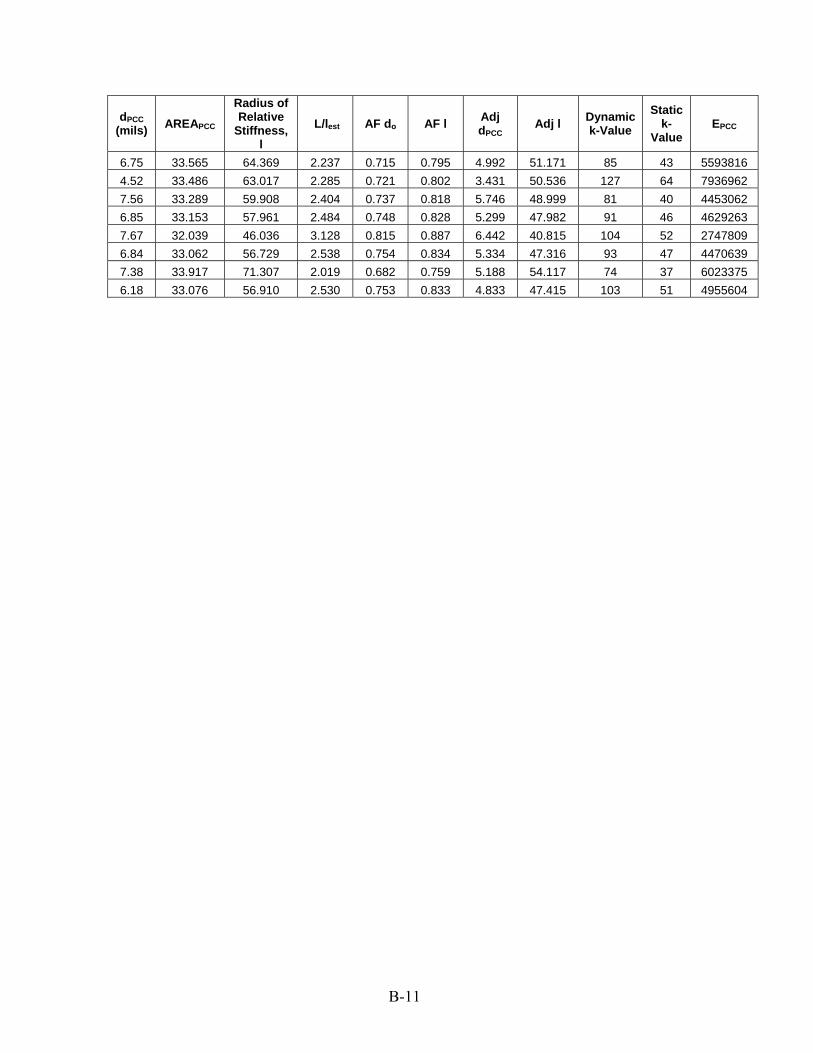
dPCC (mils) AREAPCC

Radius of Relative

Stiffness, l

L/lest AF do AF l Adj dPCC

Adj l Dynamic k-Value

Static k-

Value EPCC

6.75 33.565 64.369 2.237 0.715 0.795 4.992 51.171 85 43 5593816 4.52 33.486 63.017 2.285 0.721 0.802 3.431 50.536 127 64 7936962 7.56 33.289 59.908 2.404 0.737 0.818 5.746 48.999 81 40 4453062 6.85 33.153 57.961 2.484 0.748 0.828 5.299 47.982 91 46 4629263 7.67 32.039 46.036 3.128 0.815 0.887 6.442 40.815 104 52 2747809 6.84 33.062 56.729 2.538 0.754 0.834 5.334 47.316 93 47 4470639 7.38 33.917 71.307 2.019 0.682 0.759 5.188 54.117 74 37 6023375 6.18 33.076 56.910 2.530 0.753 0.833 4.833 47.415 103 51 4955604

B-11

Cum

mul

ativ

e %

Cummulative %,Eastbound Lane

Bonded Unbonded

100.00%

90.00%

80.00%

70.00%

60.00%

50.00%

40.00%

30.00%

20.00%

10.00%

0.00% 0 2000000 4000000 6000000 8000000 10000000 12000000

PCC Elastic modulus

B-12

Table B.3. CDOT whitetopping thickness for 20-year traffic prediction (bonded– eastbound lane)

Colorado DOT Whitetopping Design (AI, Eff, Winter)

Bonded Slabs

EAC= 1359876 PCC Poisson= 0.15 Trial Thickness= 3.5

tBase= 16.9 ACC Poisson= 0.35 Joint Spacing= 60 k= 57 Temperature Differential= 1.3 Existing Asphalt Fatigue= 30

EPCC= 6000000 N.A.= 7.08 PAC= 5.62

MR= 650 le= 75.75 VV= 2.74 L/le= .079

Axle Load, kips

Critical Concrete Stresses and Asphalt Strains Load Induced Bond Adjustment Loss of Support Adjustment

Stress, psi Microstrain Stress, psi Microstrain Stress, psi Microstrain 1 2 3 4 5 6 7

Single Axles 35 1 25 1 22 1 22 30 0 22 1 19 1 19 26 0 19 1 16 1 16 24 0 17 1 15 1 15 22 0 16 1 13 1 13 20 0 14 0 12 1 12 18 0 13 0 11 0 11 16 0 12 0 10 0 10 12 0 9 0 7 0 7 8 0 6 0 4 0 4 7 0 5 0 4 0 4 3 0 2 0 1 0 1

Tandem Axles 60 0 17 1 15 1 15 55 0 16 1 13 1 13 50 0 14 1 12 1 12 46 0 13 0 11 1 11 44 0 13 0 10 0 10 42 0 12 0 10 0 10 40 0 11 0 9 0 9 38 0 11 0 9 0 9 36 0 10 0 8 0 8 34 0 10 0 8 0 8 32 0 9 0 7 0 7 30 0 9 0 7 0 7

B-13

Axle

Load,

kips

Expected

Repetitions

Concrete Fatigue Analysis Asphalt Fatigue Analysis

Concrete Stress Ratio

Allowable Repetitions,

N

Fatigue Percent,

%

Asphalt

Microstrain

Allowable

Repetitions, N

Fatigue Percent,

%

1 8 9 10 11 12 13 14

Single Axles

Percent Asphalt Concrete Fatigue Life Previously

Consumed: 30 35 0 0.001 Unlimited 0.0 22 691588514 0.0 30 504 0.001 Unlimited 0.0 19 1171064542 0.0 26 0 0.001 Unlimited 0.0 16 1915289124 0.0 24 3961 0.001 Unlimited 0.0 15 2525652662 0.0 22 11702 0.001 Unlimited 0.0 13 3416249537 0.0 20 38322 0.001 Unlimited 0.0 12 4764277409 0.0 18 79837 0.001 Unlimited 0.0 11 6897740578 0.0 16 242208 0.001 Unlimited 0.0 10 10466725758 0.0 12 1235348 0.000 Unlimited 0.0 7 29512088266 0.0 8 165948 0.000 Unlimited 0.0 4 135205019314 0.0 7 4238911 0.000 Unlimited 0.0 4 228171366685 0.0 3 12592840 0.000 Unlimited 0.0 1 10714536949257 0.0

Tandem Axles 60 3589 0.001 Unlimited 0.0 15 2622446134 0.0 55 1794 0.001 Unlimited 0.0 13 3547819359 0.0 50 4988 0.001 Unlimited 0.0 12 4948854914 0.0 46 20709 0.001 Unlimited 0.0 11 6632642204 0.0 44 3590 0.001 Unlimited 0.0 10 7758738720 0.0 42 18149 0.001 Unlimited 0.0 10 9147555310 0.0 40 31109 0.001 Unlimited 0.0 9 10878969089 0.0 38 85463 0.001 Unlimited 0.0 9 13063473215 0.0 36 120720 0.001 Unlimited 0.0 8 15856648407 0.0 34 178092 0.001 Unlimited 0.0 8 19481945019 0.0 32 105799 0.001 Unlimited 0.0 7 24267516006 0.0 30 219452 0.001 Unlimited 0.0 7 30707580046 0.0

Total Concrete

Fatigue, % = 0.0 Total Asphalt

Fatigue, %= 30.0

B-14

Table B.4. CDOT whitetopping thickness for 20-year traffic prediction (unbonded– eastbound lane)

Colorado DOT Whitetopping Design (AI, Eff, Winter)

Unbonded Slabs

EBase= 1359876 PCC Poisson= 0.15 Trial Thickness= 4.5

tBase= 15.4 ACC Poisson= 0.35 Joint Spacing= 6 k= 52 Temperature Differential= 1.3 Existing Asphalt Fatigue= 30

EPCC= 7850000 N.A.= 5.95 PAC= 5.62

MR= 650 le= 78.35 VV= 2.74 L/le= 0.08

Axle Load, kips

Critical Concrete Stresses and Asphalt Strains Load Induced Bond Adjustment Loss of Support Adjustment

Stress, psi Microstrain Stress, psi Microstrain Stress, psi Microstrain 1 2 3 4 5 6 7

Single Axles 35 0 21 0 18 0 18 30 0 18 0 15 0 15 26 0 15 0 13 0 13 24 0 14 0 12 0 12 22 0 13 0 11 0 11 20 0 12 0 10 0 10 18 0 11 0 9 0 9 16 0 9 0 8 0 8 12 0 7 0 6 0 6 8 0 5 0 3 0 3 7 0 4 0 3 0 3 3 0 2 0 1 0 1

Tandem Axles 60 1 14 1 12 1 12 55 0 13 1 11 1 11 50 0 12 1 10 1 10 46 0 11 1 9 1 9 44 0 10 1 8 1 8 42 0 10 1 8 1 8 40 0 9 1 8 1 8 38 0 9 0 7 1 7 36 0 8 0 7 0 7 34 0 8 0 6 0 6 32 0 7 0 6 0 6 30 0 7 0 5 0 5

B-15

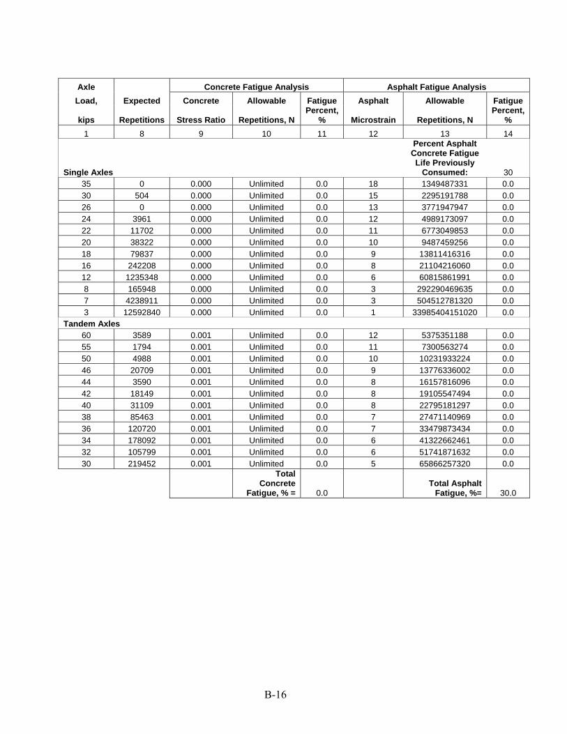
Axle Load,

kips

Expected

Repetitions

Concrete Fatigue Analysis Asphalt Fatigue Analysis Concrete

Stress Ratio

Allowable

Repetitions, N

Fatigue Percent,

%

Asphalt

Microstrain

Allowable

Repetitions, N

Fatigue Percent,

% 1 8 9 10 11 12 13 14

Single Axles

Percent Asphalt Concrete Fatigue Life Previously

Consumed: 30 35 0 0.000 Unlimited 0.0 18 1349487331 0.0 30 504 0.000 Unlimited 0.0 15 2295191788 0.0 26 0 0.000 Unlimited 0.0 13 3771947947 0.0 24 3961 0.000 Unlimited 0.0 12 4989173097 0.0 22 11702 0.000 Unlimited 0.0 11 6773049853 0.0 20 38322 0.000 Unlimited 0.0 10 9487459256 0.0 18 79837 0.000 Unlimited 0.0 9 13811416316 0.0 16 242208 0.000 Unlimited 0.0 8 21104216060 0.0 12 1235348 0.000 Unlimited 0.0 6 60815861991 0.0 8 165948 0.000 Unlimited 0.0 3 292290469635 0.0 7 4238911 0.000 Unlimited 0.0 3 504512781320 0.0 3 12592840 0.000 Unlimited 0.0 1 33985404151020 0.0

Tandem Axles 60 3589 0.001 Unlimited 0.0 12 5375351188 0.0 55 1794 0.001 Unlimited 0.0 11 7300563274 0.0 50 4988 0.001 Unlimited 0.0 10 10231933224 0.0 46 20709 0.001 Unlimited 0.0 9 13776336002 0.0 44 3590 0.001 Unlimited 0.0 8 16157816096 0.0 42 18149 0.001 Unlimited 0.0 8 19105547494 0.0 40 31109 0.001 Unlimited 0.0 8 22795181297 0.0 38 85463 0.001 Unlimited 0.0 7 27471140969 0.0 36 120720 0.001 Unlimited 0.0 7 33479873434 0.0 34 178092 0.001 Unlimited 0.0 6 41322662461 0.0 32 105799 0.001 Unlimited 0.0 6 51741871632 0.0 30 219452 0.001 Unlimited 0.0 5 65866257320 0.0

Total Concrete

Fatigue, % = 0.0 Total Asphalt

Fatigue, %= 30.0

B-16

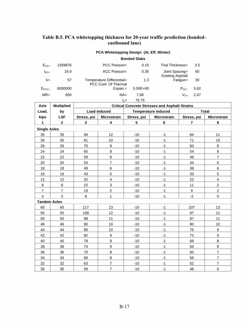
Table B.5. PCA whitetopping thickness for 20-year traffic prediction (bonded– eastbound lane)

PCA Whitetopping Design (AI, Eff, Winter)

Bonded Slabs

EAC= 1359876 PCC Poisson= 0.15 Trial Thickness= 3.5

tAC= 16.9 ACC Poisson= 0.35 Joint Spacing= 60 Existing Asphalt

k= 57 Temperature Differential= 1.3 Fatigue= 30 PCC Coef. Of Thermal

EPCC= 6000000 Expan.= 5.50E+00 PAC= 5.62

MR= 650 NA= 7.08 VV= 2.47 le = 75.75

AxleLoad, kips

1

Multiplied by

LSF 2

Critical Concrete Stresses and Asphalt Strains Load Induced Temperature Induced Total

Stress, psi Microstrain Stress, psi Microstrain Stress, psi Microstrain 3 4 5 6 7 8

Single Axles 35 35 94 12 -10 -1 84 11 30 30 81 10 -10 -1 71 10 26 26 70 9 -10 -1 60 8 24 24 65 8 -10 -1 54 8 22 22 59 8 -10 -1 49 7 20 20 54 7 -10 -1 44 6 18 18 49 6 -10 -1 38 6 16 16 43 6 -10 -1 33 5 12 12 32 4 -10 -1 22 4 8 8 22 3 -10 -1 11 2 7 7 19 2 -10 -1 9 2 3 3 8 1 -10 -1 -2 0

Tandem Axles 60 60 117 13 -10 -1 107 13 55 55 108 12 -10 -1 97 12 50 50 98 11 -10 -1 87 11 46 46 90 10 -10 -1 80 10 44 44 86 10 -10 -1 76 9 42 42 82 9 -10 -1 72 9 40 40 78 9 -10 -1 68 8 38 38 74 9 -10 -1 64 8 36 36 70 8 -10 -1 60 7 34 34 66 8 -10 -1 56 7 32 32 63 7 -10 -1 52 7 30 30 59 7 -10 -1 48 6

B-17

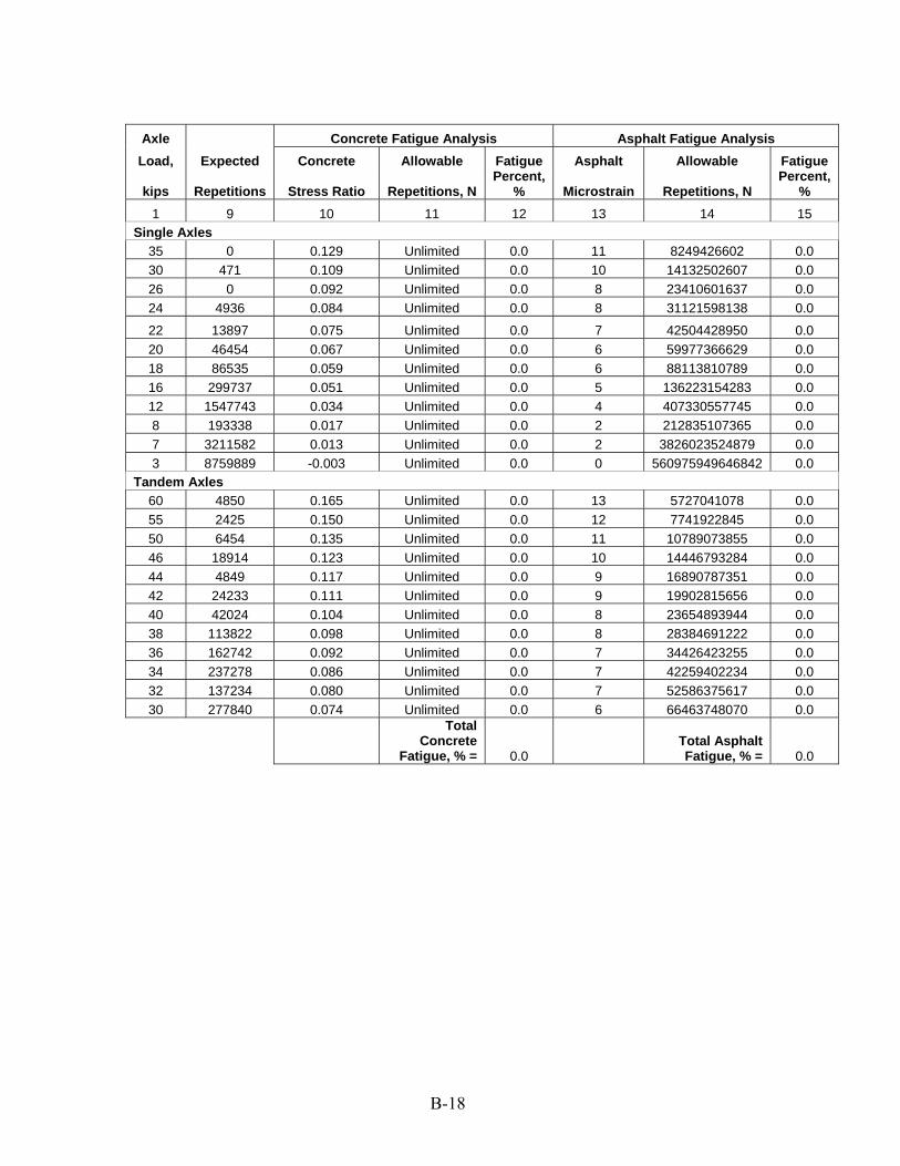
Axle Load,

kips

Expected

Repetitions

Concrete Fatigue Analysis Asphalt Fatigue Analysis Concrete

Stress Ratio

Allowable

Repetitions, N

Fatigue Percent,

%

Asphalt

Microstrain

Allowable

Repetitions, N

Fatigue Percent,

% 1 9 10 11 12 13 14 15

Single Axles 35 0 0.129 Unlimited 0.0 11 8249426602 0.0 30 471 0.109 Unlimited 0.0 10 14132502607 0.0 26 0 0.092 Unlimited 0.0 8 23410601637 0.0 24 4936 0.084 Unlimited 0.0 8 31121598138 0.0

22 13897 0.075 Unlimited 0.0 7 42504428950 0.0 20 46454 0.067 Unlimited 0.0 6 59977366629 0.0 18 86535 0.059 Unlimited 0.0 6 88113810789 0.0 16 299737 0.051 Unlimited 0.0 5 136223154283 0.0 12 1547743 0.034 Unlimited 0.0 4 407330557745 0.0 8 193338 0.017 Unlimited 0.0 2 212835107365 0.0 7 3211582 0.013 Unlimited 0.0 2 3826023524879 0.0 3 8759889 -0.003 Unlimited 0.0 0 560975949646842 0.0

Tandem Axles 60 4850 0.165 Unlimited 0.0 13 5727041078 0.0 55 2425 0.150 Unlimited 0.0 12 7741922845 0.0 50 6454 0.135 Unlimited 0.0 11 10789073855 0.0 46 18914 0.123 Unlimited 0.0 10 14446793284 0.0 44 4849 0.117 Unlimited 0.0 9 16890787351 0.0 42 24233 0.111 Unlimited 0.0 9 19902815656 0.0 40 42024 0.104 Unlimited 0.0 8 23654893944 0.0 38 113822 0.098 Unlimited 0.0 8 28384691222 0.0 36 162742 0.092 Unlimited 0.0 7 34426423255 0.0 34 237278 0.086 Unlimited 0.0 7 42259402234 0.0 32 137234 0.080 Unlimited 0.0 7 52586375617 0.0 30 277840 0.074 Unlimited 0.0 6 66463748070 0.0

Total Concrete

Fatigue, % = 0.0 Total Asphalt Fatigue, % = 0.0

B-18

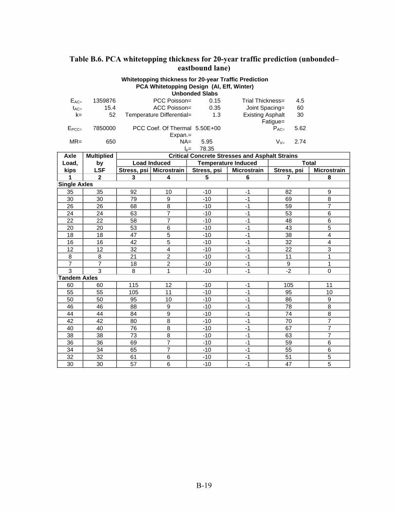
Table B.6. PCA whitetopping thickness for 20-year traffic prediction (unbonded– eastbound lane)

Whitetopping thickness for 20-year Traffic PredictionPCA Whitetopping Design (AI, Eff, Winter)

Unbonded SlabsEAC= 1359876 PCC Poisson= 0.15 Trial Thickness= 4.5 tAC= 15.4 ACC Poisson= 0.35 Joint Spacing= 60 k= 52 Temperature Differential= 1.3 Existing Asphalt 30

Fatigue= EPCC= 7850000 PCC Coef. Of Thermal 5.50E+00 PAC= 5.62

Expan.= MR= 650 NA= 5.95 VV= 2.74

le= 78.35 Axle

Load, kips

Multiplied by

LSF

Critical Concrete Stresses and Asphalt Strains Load Induced Temperature Induced Total

Stress, psi Microstrain Stress, psi Microstrain Stress, psi Microstrain 1 2 3 4 5 6 7 8

Single Axles 35 35 92 10 -10 -1 82 9 30 30 79 9 -10 -1 69 8 26 26 68 8 -10 -1 59 7 24 24 63 7 -10 -1 53 6 22 22 58 7 -10 -1 48 6 20 20 53 6 -10 -1 43 5 18 18 47 5 -10 -1 38 4 16 16 42 5 -10 -1 32 4 12 12 32 4 -10 -1 22 3 8 8 21 2 -10 -1 11 1 7 7 18 2 -10 -1 9 1 3 3 8 1 -10 -1 -2 0

Tandem Axles 60 60 115 12 -10 -1 105 11 55 55 105 11 -10 -1 95 10 50 50 95 10 -10 -1 86 9 46 46 88 9 -10 -1 78 8 44 44 84 9 -10 -1 74 8 42 42 80 8 -10 -1 70 7 40 40 76 8 -10 -1 67 7 38 38 73 8 -10 -1 63 7 36 36 69 7 -10 -1 59 6 34 34 65 7 -10 -1 55 6 32 32 61 6 -10 -1 51 5 30 30 57 6 -10 -1 47 5

B-19

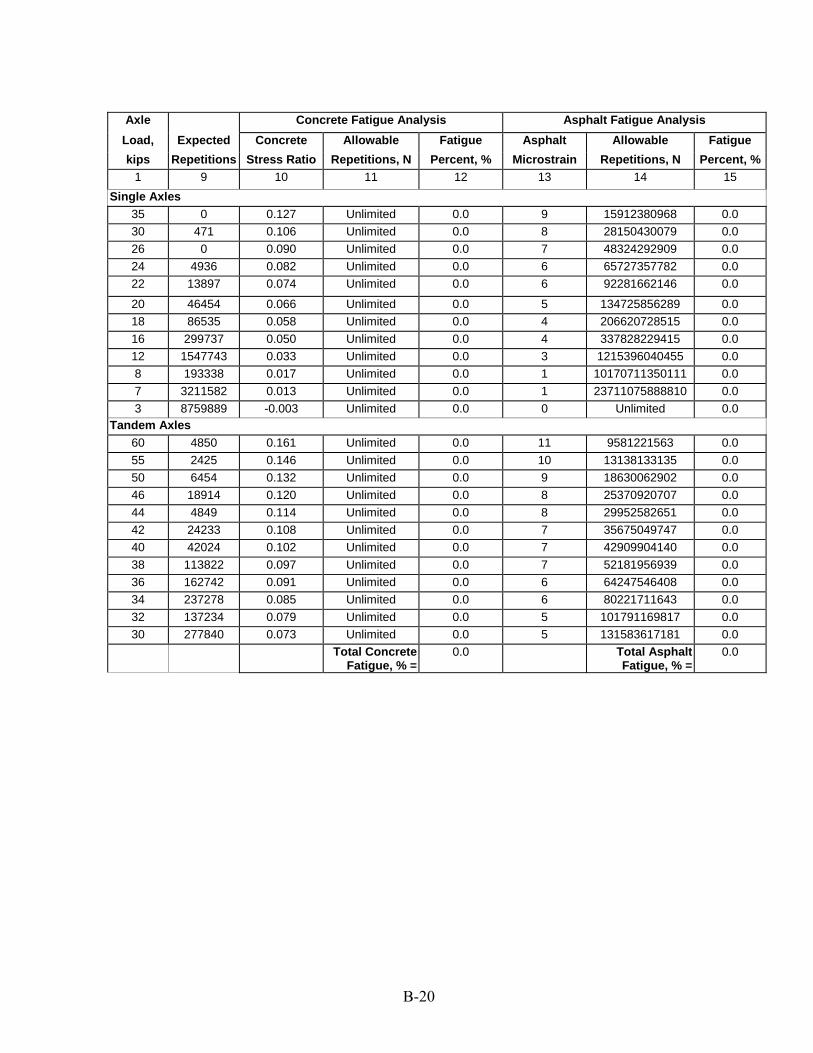
Axle Load, kips

Expected Repetitions

Concrete Fatigue Analysis Asphalt Fatigue Analysis Concrete

Stress Ratio Allowable

Repetitions, N Fatigue

Percent, % Asphalt

Microstrain Allowable

Repetitions, N Fatigue

Percent, % 1 9 10 11 12 13 14 15

Single Axles 35 0 0.127 Unlimited 0.0 9 15912380968 0.0 30 471 0.106 Unlimited 0.0 8 28150430079 0.0 26 0 0.090 Unlimited 0.0 7 48324292909 0.0 24 4936 0.082 Unlimited 0.0 6 65727357782 0.0 22 13897 0.074 Unlimited 0.0 6 92281662146 0.0

20 46454 0.066 Unlimited 0.0 5 134725856289 0.0 18 86535 0.058 Unlimited 0.0 4 206620728515 0.0 16 299737 0.050 Unlimited 0.0 4 337828229415 0.0 12 1547743 0.033 Unlimited 0.0 3 1215396040455 0.0 8 193338 0.017 Unlimited 0.0 1 10170711350111 0.0 7 3211582 0.013 Unlimited 0.0 1 23711075888810 0.0 3 8759889 -0.003 Unlimited 0.0 0 Unlimited 0.0

Tandem Axles 60 4850 0.161 Unlimited 0.0 11 9581221563 0.0 55 2425 0.146 Unlimited 0.0 10 13138133135 0.0 50 6454 0.132 Unlimited 0.0 9 18630062902 0.0 46 18914 0.120 Unlimited 0.0 8 25370920707 0.0 44 4849 0.114 Unlimited 0.0 8 29952582651 0.0 42 24233 0.108 Unlimited 0.0 7 35675049747 0.0 40 42024 0.102 Unlimited 0.0 7 42909904140 0.0 38 113822 0.097 Unlimited 0.0 7 52181956939 0.0 36 162742 0.091 Unlimited 0.0 6 64247546408 0.0 34 237278 0.085 Unlimited 0.0 6 80221711643 0.0 32 137234 0.079 Unlimited 0.0 5 101791169817 0.0 30 277840 0.073 Unlimited 0.0 5 131583617181 0.0

Total Concrete Fatigue, % =

0.0 Total Asphalt Fatigue, % =

0.0

B-20

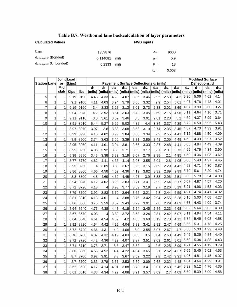
Table B.7. Westbound lane backcalculation of layer parameters Calculated Values FWD inputs

EACC 1359876 P= 9000 do compress (Bonded) 0.114081 mils a= 5.9 do compress (Unbonded) 0.2333 mils F= 18

tw= 0.003

Station Lane Joint

or Load (kips) Pavement Surface Deflections di (mils)

Modified Surface Deflections, di

Mid slab Kips lbs

d0 (mils)

d8 (mils)

d12 (mils)

d18 (mils)

d24 (mils)

d36 (mils)

d48 (mils)

d60 (mils)

d-12 (mils)

d0 (mils)

d12 (mils)

d24 (mils)

d36 (mils)

5 1 1 9.19 9190 4.43 4.33 4.23 4.07 3.86 3.46 2.95 2.53 4.2 5.30 5.06 4.62 4.14

6 1 1 9.1 9100 4.11 4.03 3.94 3.79 3.66 3.32 2.9 2.54 5.61 4.97 4.76 4.43 4.01

7 1 1 9.19 9190 3.4 3.33 3.26 3.13 3.01 2.73 2.38 2.01 3.69 4.07 3.90 3.60 3.27

8 1 1 9.04 9040 4.2 3.92 3.81 3.63 3.42 3.05 2.59 2.15 4.96 5.11 4.64 4.16 3.71

9 1 1 9.11 9110 3.8 3.61 3.62 3.46 3.3 3.01 2.61 2.28 5.2 4.59 4.37 3.99 3.64

10 1 1 8.91 8910 5.44 5.27 5.26 5.02 4.82 4.4 3.84 3.37 4.29 6.72 6.50 5.95 5.43

11 1 1 8.97 8970 3.97 3.8 3.83 3.68 3.53 3.19 2.74 2.35 3.45 4.87 4.70 4.33 3.91

12 1 1 8.99 8990 4.18 4.02 3.99 3.84 3.68 3.34 2.9 2.55 4.41 5.12 4.88 4.50 4.09

13 1 1 8.9 8900 3.74 3.63 3.55 3.39 3.21 2.85 2.41 2.05 4.49 4.62 4.39 3.97 3.52

14 1 1 8.95 8950 4.11 4.01 3.94 3.81 3.65 3.33 2.87 2.48 4.41 5.05 4.84 4.49 4.09

15 1 1 8.95 8950 4.06 3.92 3.86 3.71 3.53 3.17 2.7 2.31 3.73 4.99 4.75 4.34 3.90

16 1 1 8.38 8380 3.43 3.38 3.32 3.19 3.07 2.76 2.38 2.1 4.95 4.50 4.36 4.03 3.62

17 1 1 8.77 8770 4.62 4.41 4.33 4.14 3.96 3.55 3.04 2.6 4.95 5.80 5.43 4.97 4.45

18 1 1 8.95 8950 4 3.89 3.83 3.67 3.5 3.15 2.69 2.29 4.42 4.92 4.71 4.30 3.87

19 1 1 8.86 8860 4.66 4.58 4.52 4.36 4.19 3.82 3.32 2.89 2.99 5.79 5.61 5.20 4.74

20 1 1 8.8 8800 4.8 4.69 4.62 4.45 4.27 3.9 3.38 2.96 2.51 6.00 5.78 5.34 4.88

21 1 1 8.94 8940 4.12 4.02 3.96 3.83 3.71 3.41 2.99 2.64 6.17 5.07 4.87 4.57 4.20

22 1 1 8.72 8720 4.13 4 3.93 3.77 3.59 3.19 2.7 2.26 5.19 5.21 4.96 4.53 4.03

23 1 1 8.79 8790 3.92 3.83 3.79 3.64 3.52 3.21 2.8 2.44 5.59 4.91 4.74 4.41 4.02

24 1 1 8.81 8810 4.13 4.01 4 3.88 3.75 3.42 2.94 2.55 5.28 5.16 5.00 4.68 4.27

25 1 1 8.86 8860 3.75 3.59 3.57 3.43 3.29 3.01 2.6 2.29 4.69 4.66 4.43 4.09 3.74

26 1 1 8.64 8640 4.73 4.38 4.43 4.18 3.94 3.45 2.84 2.33 4.68 6.02 5.64 5.02 4.39

27 1 1 8.67 8670 4.03 4 3.89 3.72 3.58 3.24 2.81 2.42 5.07 5.11 4.94 4.54 4.11

28 1 1 8.84 8840 4.61 4.54 4.39 4.2 4.03 3.68 3.19 2.78 4.12 5.74 5.46 5.02 4.58

29 1 1 8.82 8820 4.54 4.42 4.26 4.04 3.83 3.41 2.92 2.47 4.69 5.66 5.31 4.78 4.25

30 1 1 8.72 8720 4.36 4.31 4.2 4.06 3.9 3.55 3.07 2.67 4.7 5.50 5.30 4.92 4.48

31 1 1 8.76 8760 4.37 4.32 4.19 4.03 3.85 3.5 3.04 2.63 4.49 5.49 5.26 4.84 4.40

32 1 1 8.72 8720 4.42 4.36 4.23 4.07 3.87 3.51 3.03 2.61 5.01 5.58 5.34 4.88 4.43

33 1 1 8.71 8710 3.73 3.71 3.6 3.47 3.32 3 2.6 2.25 3.99 4.71 4.55 4.19 3.79

34 1 1 8.86 8860 4.55 4.52 4.4 4.22 4.04 3.65 3.1 2.62 4.37 5.65 5.46 5.02 4.53

35 1 1 8.7 8700 3.92 3.91 3.8 3.67 3.52 3.22 2.8 2.42 3.31 4.96 4.81 4.45 4.07

36 1 1 8.7 8700 3.83 3.78 3.67 3.53 3.39 3.09 2.68 2.32 4.48 4.84 4.64 4.29 3.91

37 1 1 8.62 8620 4.17 4.14 4.01 3.88 3.73 3.41 3.01 2.63 5.45 5.32 5.12 4.76 4.35

38 1 1 8.61 8610 4.38 4.34 4.22 4.08 3.91 3.57 3.09 2.7 4.09 5.60 5.39 5.00 4.56

B-21

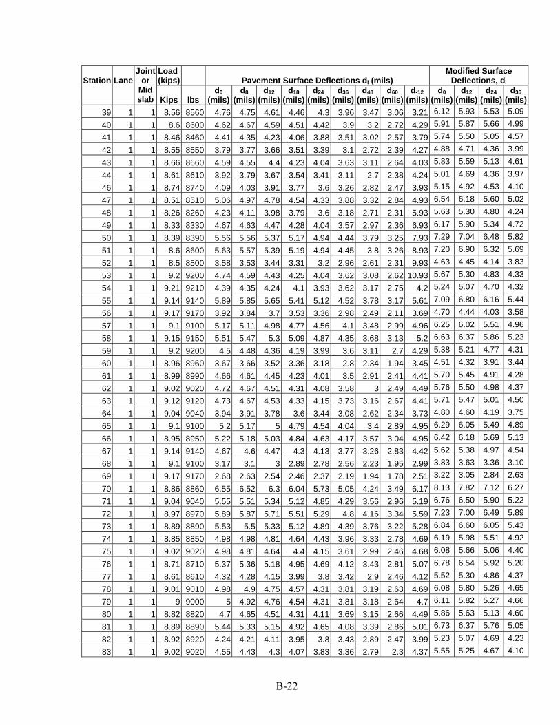
Station Lane Joint

or Load (kips) Pavement Surface Deflections di (mils)

Modified Surface Deflections, di

Mid slab Kips lbs

d0 (mils)

d8 (mils)

d12 (mils)

d18 (mils)

d24 (mils)

d36 (mils)

d48 (mils)

d60 (mils)

d-12 (mils)

d0 (mils)

d12 (mils)

d24 (mils)

d36 (mils)

39 1 1 8.56 8560 4.76 4.75 4.61 4.46 4.3 3.96 3.47 3.06 3.21 6.12 5.93 5.53 5.09

40 1 1 8.6 8600 4.62 4.67 4.59 4.51 4.42 3.9 3.2 2.72 4.29 5.91 5.87 5.66 4.99

41 1 1 8.46 8460 4.41 4.35 4.23 4.06 3.88 3.51 3.02 2.57 3.79 5.74 5.50 5.05 4.57

42 1 1 8.55 8550 3.79 3.77 3.66 3.51 3.39 3.1 2.72 2.39 4.27 4.88 4.71 4.36 3.99

43 1 1 8.66 8660 4.59 4.55 4.4 4.23 4.04 3.63 3.11 2.64 4.03 5.83 5.59 5.13 4.61

44 1 1 8.61 8610 3.92 3.79 3.67 3.54 3.41 3.11 2.7 2.38 4.24 5.01 4.69 4.36 3.97

46 1 1 8.74 8740 4.09 4.03 3.91 3.77 3.6 3.26 2.82 2.47 3.93 5.15 4.92 4.53 4.10

47 1 1 8.51 8510 5.06 4.97 4.78 4.54 4.33 3.88 3.32 2.84 4.93 6.54 6.18 5.60 5.02

48 1 1 8.26 8260 4.23 4.11 3.98 3.79 3.6 3.18 2.71 2.31 5.93 5.63 5.30 4.80 4.24

49 1 1 8.33 8330 4.67 4.63 4.47 4.28 4.04 3.57 2.97 2.36 6.93 6.17 5.90 5.34 4.72

50 1 1 8.39 8390 5.56 5.56 5.37 5.17 4.94 4.44 3.79 3.25 7.93 7.29 7.04 6.48 5.82

51 1 1 8.6 8600 5.63 5.57 5.39 5.19 4.94 4.45 3.8 3.26 8.93 7.20 6.90 6.32 5.69

52 1 1 8.5 8500 3.58 3.53 3.44 3.31 3.2 2.96 2.61 2.31 9.93 4.63 4.45 4.14 3.83

53 1 1 9.2 9200 4.74 4.59 4.43 4.25 4.04 3.62 3.08 2.62 10.93 5.67 5.30 4.83 4.33

54 1 1 9.21 9210 4.39 4.35 4.24 4.1 3.93 3.62 3.17 2.75 4.2 5.24 5.07 4.70 4.32

55 1 1 9.14 9140 5.89 5.85 5.65 5.41 5.12 4.52 3.78 3.17 5.61 7.09 6.80 6.16 5.44

56 1 1 9.17 9170 3.92 3.84 3.7 3.53 3.36 2.98 2.49 2.11 3.69 4.70 4.44 4.03 3.58

57 1 1 9.1 9100 5.17 5.11 4.98 4.77 4.56 4.1 3.48 2.99 4.96 6.25 6.02 5.51 4.96

58 1 1 9.15 9150 5.51 5.47 5.3 5.09 4.87 4.35 3.68 3.13 5.2 6.63 6.37 5.86 5.23

59 1 1 9.2 9200 4.5 4.48 4.36 4.19 3.99 3.6 3.11 2.7 4.29 5.38 5.21 4.77 4.31

60 1 1 8.96 8960 3.67 3.66 3.52 3.36 3.18 2.8 2.34 1.94 3.45 4.51 4.32 3.91 3.44

61 1 1 8.99 8990 4.66 4.61 4.45 4.23 4.01 3.5 2.91 2.41 4.41 5.70 5.45 4.91 4.28

62 1 1 9.02 9020 4.72 4.67 4.51 4.31 4.08 3.58 3 2.49 4.49 5.76 5.50 4.98 4.37

63 1 1 9.12 9120 4.73 4.67 4.53 4.33 4.15 3.73 3.16 2.67 4.41 5.71 5.47 5.01 4.50

64 1 1 9.04 9040 3.94 3.91 3.78 3.6 3.44 3.08 2.62 2.34 3.73 4.80 4.60 4.19 3.75

65 1 1 9.1 9100 5.2 5.17 5 4.79 4.54 4.04 3.4 2.89 4.95 6.29 6.05 5.49 4.89

66 1 1 8.95 8950 5.22 5.18 5.03 4.84 4.63 4.17 3.57 3.04 4.95 6.42 6.18 5.69 5.13

67 1 1 9.14 9140 4.67 4.6 4.47 4.3 4.13 3.77 3.26 2.83 4.42 5.62 5.38 4.97 4.54

68 1 1 9.1 9100 3.17 3.1 3 2.89 2.78 2.56 2.23 1.95 2.99 3.83 3.63 3.36 3.10

69 1 1 9.17 9170 2.68 2.63 2.54 2.46 2.37 2.19 1.94 1.78 2.51 3.22 3.05 2.84 2.63

70 1 1 8.86 8860 6.55 6.52 6.3 6.04 5.73 5.05 4.24 3.49 6.17 8.13 7.82 7.12 6.27

71 1 1 9.04 9040 5.55 5.51 5.34 5.12 4.85 4.29 3.56 2.96 5.19 6.76 6.50 5.90 5.22

72 1 1 8.97 8970 5.89 5.87 5.71 5.51 5.29 4.8 4.16 3.34 5.59 7.23 7.00 6.49 5.89

73 1 1 8.89 8890 5.53 5.5 5.33 5.12 4.89 4.39 3.76 3.22 5.28 6.84 6.60 6.05 5.43

74 1 1 8.85 8850 4.98 4.98 4.81 4.64 4.43 3.96 3.33 2.78 4.69 6.19 5.98 5.51 4.92

75 1 1 9.02 9020 4.98 4.81 4.64 4.4 4.15 3.61 2.99 2.46 4.68 6.08 5.66 5.06 4.40

76 1 1 8.71 8710 5.37 5.36 5.18 4.95 4.69 4.12 3.43 2.81 5.07 6.78 6.54 5.92 5.20

77 1 1 8.61 8610 4.32 4.28 4.15 3.99 3.8 3.42 2.9 2.46 4.12 5.52 5.30 4.86 4.37

78 1 1 9.01 9010 4.98 4.9 4.75 4.57 4.31 3.81 3.19 2.63 4.69 6.08 5.80 5.26 4.65

79 1 1 9 9000 5 4.92 4.76 4.54 4.31 3.81 3.18 2.64 4.7 6.11 5.82 5.27 4.66

80 1 1 8.82 8820 4.7 4.65 4.51 4.31 4.11 3.69 3.15 2.66 4.49 5.86 5.63 5.13 4.60

81 1 1 8.89 8890 5.44 5.33 5.15 4.92 4.65 4.08 3.39 2.86 5.01 6.73 6.37 5.76 5.05

82 1 1 8.92 8920 4.24 4.21 4.11 3.95 3.8 3.43 2.89 2.47 3.99 5.23 5.07 4.69 4.23

83 1 1 9.02 9020 4.55 4.43 4.3 4.07 3.83 3.36 2.79 2.3 4.37 5.55 5.25 4.67 4.10

B-22

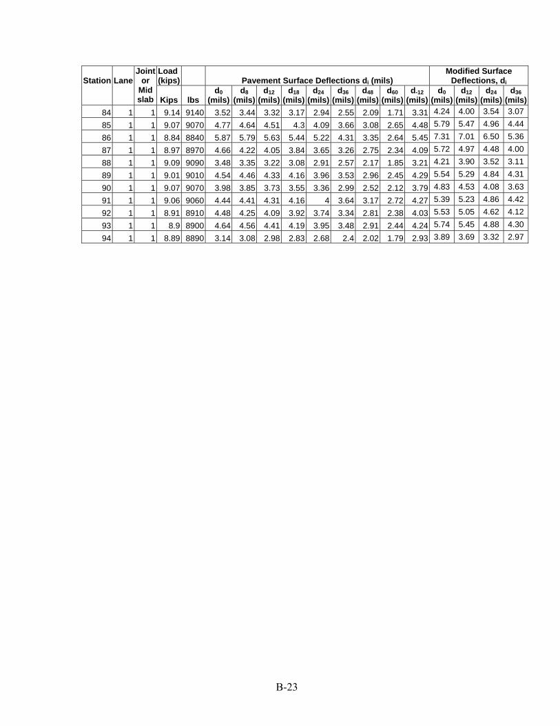
Station Lane Joint

or Load (kips) Pavement Surface Deflections di (mils)

Modified Surface Deflections, di

Mid slab Kips lbs

d0 (mils)

d8 (mils)

d12 (mils)

d18 (mils)

d24 (mils)

d36 (mils)

d48 (mils)

d60 (mils)

d-12 (mils)

d0 (mils)

d12 (mils)

d24 (mils)

d36 (mils)

84 1 1 9.14 9140 3.52 3.44 3.32 3.17 2.94 2.55 2.09 1.71 3.31 4.24 4.00 3.54 3.07

85 1 1 9.07 9070 4.77 4.64 4.51 4.3 4.09 3.66 3.08 2.65 4.48 5.79 5.47 4.96 4.44

86 1 1 8.84 8840 5.87 5.79 5.63 5.44 5.22 4.31 3.35 2.64 5.45 7.31 7.01 6.50 5.36

87 1 1 8.97 8970 4.66 4.22 4.05 3.84 3.65 3.26 2.75 2.34 4.09 5.72 4.97 4.48 4.00

88 1 1 9.09 9090 3.48 3.35 3.22 3.08 2.91 2.57 2.17 1.85 3.21 4.21 3.90 3.52 3.11

89 1 1 9.01 9010 4.54 4.46 4.33 4.16 3.96 3.53 2.96 2.45 4.29 5.54 5.29 4.84 4.31

90 1 1 9.07 9070 3.98 3.85 3.73 3.55 3.36 2.99 2.52 2.12 3.79 4.83 4.53 4.08 3.63

91 1 1 9.06 9060 4.44 4.41 4.31 4.16 4 3.64 3.17 2.72 4.27 5.39 5.23 4.86 4.42

92 1 1 8.91 8910 4.48 4.25 4.09 3.92 3.74 3.34 2.81 2.38 4.03 5.53 5.05 4.62 4.12

93 1 1 8.9 8900 4.64 4.56 4.41 4.19 3.95 3.48 2.91 2.44 4.24 5.74 5.45 4.88 4.30

94 1 1 8.89 8890 3.14 3.08 2.98 2.83 2.68 2.4 2.02 1.79 2.93 3.89 3.69 3.32 2.97

B-23

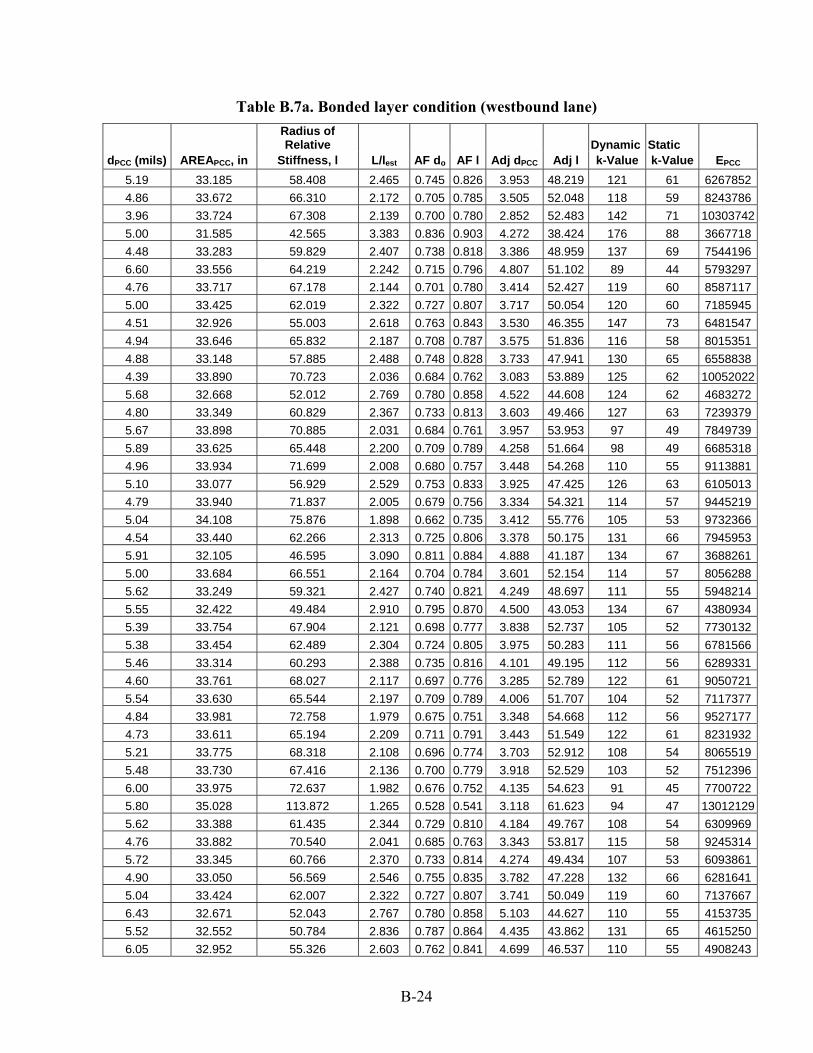
Table B.7a. Bonded layer condition (westbound lane)

dPCC (mils) AREAPCC, in

Radius of Relative

Stiffness, l L/lest AF do AF l Adj dPCC Adj l Dynamic k-Value

Static k-Value EPCC

5.19 33.185 58.408 2.465 0.745 0.826 3.953 48.219 121 61 6267852 4.86 33.672 66.310 2.172 0.705 0.785 3.505 52.048 118 59 8243786 3.96 33.724 67.308 2.139 0.700 0.780 2.852 52.483 142 71 10303742 5.00 31.585 42.565 3.383 0.836 0.903 4.272 38.424 176 88 3667718 4.48 33.283 59.829 2.407 0.738 0.818 3.386 48.959 137 69 7544196 6.60 33.556 64.219 2.242 0.715 0.796 4.807 51.102 89 44 5793297 4.76 33.717 67.178 2.144 0.701 0.780 3.414 52.427 119 60 8587117 5.00 33.425 62.019 2.322 0.727 0.807 3.717 50.054 120 60 7185945 4.51 32.926 55.003 2.618 0.763 0.843 3.530 46.355 147 73 6481547 4.94 33.646 65.832 2.187 0.708 0.787 3.575 51.836 116 58 8015351 4.88 33.148 57.885 2.488 0.748 0.828 3.733 47.941 130 65 6558838 4.39 33.890 70.723 2.036 0.684 0.762 3.083 53.889 125 62 10052022 5.68 32.668 52.012 2.769 0.780 0.858 4.522 44.608 124 62 4683272 4.80 33.349 60.829 2.367 0.733 0.813 3.603 49.466 127 63 7239379 5.67 33.898 70.885 2.031 0.684 0.761 3.957 53.953 97 49 7849739 5.89 33.625 65.448 2.200 0.709 0.789 4.258 51.664 98 49 6685318 4.96 33.934 71.699 2.008 0.680 0.757 3.448 54.268 110 55 9113881 5.10 33.077 56.929 2.529 0.753 0.833 3.925 47.425 126 63 6105013 4.79 33.940 71.837 2.005 0.679 0.756 3.334 54.321 114 57 9445219 5.04 34.108 75.876 1.898 0.662 0.735 3.412 55.776 105 53 9732366 4.54 33.440 62.266 2.313 0.725 0.806 3.378 50.175 131 66 7945953 5.91 32.105 46.595 3.090 0.811 0.884 4.888 41.187 134 67 3688261 5.00 33.684 66.551 2.164 0.704 0.784 3.601 52.154 114 57 8056288 5.62 33.249 59.321 2.427 0.740 0.821 4.249 48.697 111 55 5948214 5.55 32.422 49.484 2.910 0.795 0.870 4.500 43.053 134 67 4380934 5.39 33.754 67.904 2.121 0.698 0.777 3.838 52.737 105 52 7730132 5.38 33.454 62.489 2.304 0.724 0.805 3.975 50.283 111 56 6781566 5.46 33.314 60.293 2.388 0.735 0.816 4.101 49.195 112 56 6289331 4.60 33.761 68.027 2.117 0.697 0.776 3.285 52.789 122 61 9050721 5.54 33.630 65.544 2.197 0.709 0.789 4.006 51.707 104 52 7117377 4.84 33.981 72.758 1.979 0.675 0.751 3.348 54.668 112 56 9527177 4.73 33.611 65.194 2.209 0.711 0.791 3.443 51.549 122 61 8231932 5.21 33.775 68.318 2.108 0.696 0.774 3.703 52.912 108 54 8065519 5.48 33.730 67.416 2.136 0.700 0.779 3.918 52.529 103 52 7512396 6.00 33.975 72.637 1.982 0.676 0.752 4.135 54.623 91 45 7700722 5.80 35.028 113.872 1.265 0.528 0.541 3.118 61.623 94 47 13012129 5.62 33.388 61.435 2.344 0.729 0.810 4.184 49.767 108 54 6309969 4.76 33.882 70.540 2.041 0.685 0.763 3.343 53.817 115 58 9245314 5.72 33.345 60.766 2.370 0.733 0.814 4.274 49.434 107 53 6093861 4.90 33.050 56.569 2.546 0.755 0.835 3.782 47.228 132 66 6281641 5.04 33.424 62.007 2.322 0.727 0.807 3.741 50.049 119 60 7137667 6.43 32.671 52.043 2.767 0.780 0.858 5.103 44.627 110 55 4153735 5.52 32.552 50.784 2.836 0.787 0.864 4.435 43.862 131 65 4615250 6.05 32.952 55.326 2.603 0.762 0.841 4.699 46.537 110 55 4908243

B-24

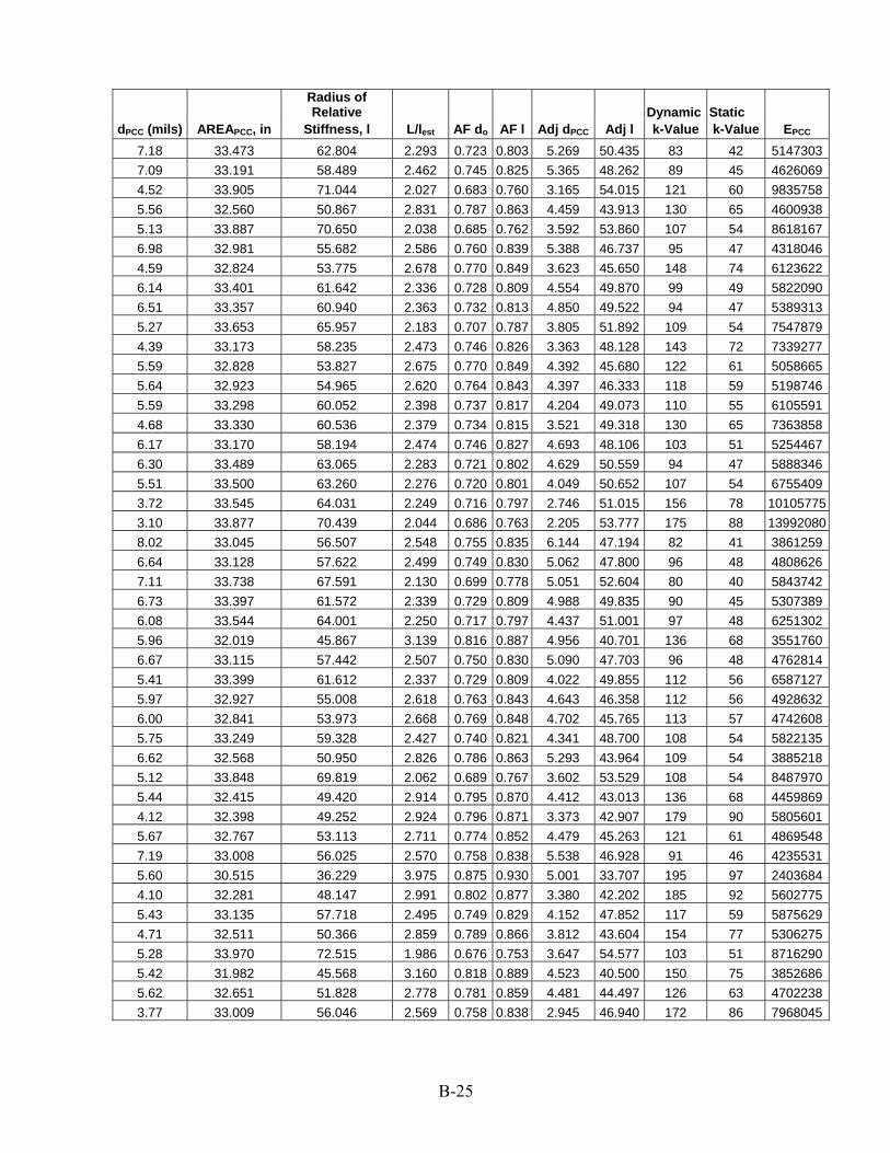
dPCC (mils) AREAPCC, in

Radius of Relative

Stiffness, l L/lest AF do AF l Adj dPCC Adj l Dynamic k-Value

Static k-Value EPCC

7.18 33.473 62.804 2.293 0.723 0.803 5.269 50.435 83 42 5147303 7.09 33.191 58.489 2.462 0.745 0.825 5.365 48.262 89 45 4626069 4.52 33.905 71.044 2.027 0.683 0.760 3.165 54.015 121 60 9835758 5.56 32.560 50.867 2.831 0.787 0.863 4.459 43.913 130 65 4600938 5.13 33.887 70.650 2.038 0.685 0.762 3.592 53.860 107 54 8618167 6.98 32.981 55.682 2.586 0.760 0.839 5.388 46.737 95 47 4318046 4.59 32.824 53.775 2.678 0.770 0.849 3.623 45.650 148 74 6123622 6.14 33.401 61.642 2.336 0.728 0.809 4.554 49.870 99 49 5822090 6.51 33.357 60.940 2.363 0.732 0.813 4.850 49.522 94 47 5389313 5.27 33.653 65.957 2.183 0.707 0.787 3.805 51.892 109 54 7547879 4.39 33.173 58.235 2.473 0.746 0.826 3.363 48.128 143 72 7339277 5.59 32.828 53.827 2.675 0.770 0.849 4.392 45.680 122 61 5058665 5.64 32.923 54.965 2.620 0.764 0.843 4.397 46.333 118 59 5198746 5.59 33.298 60.052 2.398 0.737 0.817 4.204 49.073 110 55 6105591 4.68 33.330 60.536 2.379 0.734 0.815 3.521 49.318 130 65 7363858 6.17 33.170 58.194 2.474 0.746 0.827 4.693 48.106 103 51 5254467 6.30 33.489 63.065 2.283 0.721 0.802 4.629 50.559 94 47 5888346 5.51 33.500 63.260 2.276 0.720 0.801 4.049 50.652 107 54 6755409 3.72 33.545 64.031 2.249 0.716 0.797 2.746 51.015 156 78 10105775 3.10 33.877 70.439 2.044 0.686 0.763 2.205 53.777 175 88 13992080 8.02 33.045 56.507 2.548 0.755 0.835 6.144 47.194 82 41 3861259 6.64 33.128 57.622 2.499 0.749 0.830 5.062 47.800 96 48 4808626 7.11 33.738 67.591 2.130 0.699 0.778 5.051 52.604 80 40 5843742 6.73 33.397 61.572 2.339 0.729 0.809 4.988 49.835 90 45 5307389 6.08 33.544 64.001 2.250 0.717 0.797 4.437 51.001 97 48 6251302 5.96 32.019 45.867 3.139 0.816 0.887 4.956 40.701 136 68 3551760 6.67 33.115 57.442 2.507 0.750 0.830 5.090 47.703 96 48 4762814 5.41 33.399 61.612 2.337 0.729 0.809 4.022 49.855 112 56 6587127 5.97 32.927 55.008 2.618 0.763 0.843 4.643 46.358 112 56 4928632 6.00 32.841 53.973 2.668 0.769 0.848 4.702 45.765 113 57 4742608 5.75 33.249 59.328 2.427 0.740 0.821 4.341 48.700 108 54 5822135 6.62 32.568 50.950 2.826 0.786 0.863 5.293 43.964 109 54 3885218 5.12 33.848 69.819 2.062 0.689 0.767 3.602 53.529 108 54 8487970 5.44 32.415 49.420 2.914 0.795 0.870 4.412 43.013 136 68 4459869 4.12 32.398 49.252 2.924 0.796 0.871 3.373 42.907 179 90 5805601 5.67 32.767 53.113 2.711 0.774 0.852 4.479 45.263 121 61 4869548 7.19 33.008 56.025 2.570 0.758 0.838 5.538 46.928 91 46 4235531 5.60 30.515 36.229 3.975 0.875 0.930 5.001 33.707 195 97 2403684 4.10 32.281 48.147 2.991 0.802 0.877 3.380 42.202 185 92 5602775 5.43 33.135 57.718 2.495 0.749 0.829 4.152 47.852 117 59 5875629 4.71 32.511 50.366 2.859 0.789 0.866 3.812 43.604 154 77 5306275 5.28 33.970 72.515 1.986 0.676 0.753 3.647 54.577 103 51 8716290 5.42 31.982 45.568 3.160 0.818 0.889 4.523 40.500 150 75 3852686 5.62 32.651 51.828 2.778 0.781 0.859 4.481 44.497 126 63 4702238 3.77 33.009 56.046 2.569 0.758 0.838 2.945 46.940 172 86 7968045

B-25

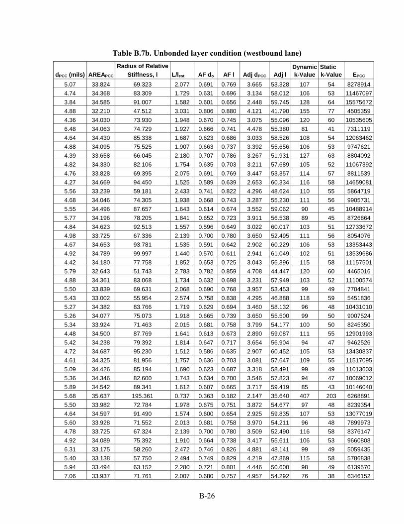
Table B.7b. Unbonded layer condition (westbound lane)

dPCC (mils) AREAPCC

Radius of Relative Stiffness, l L/lest AF do AF l Adj dPCC Adj l

Dynamic k-Value

Static k-Value EPCC

5.07 33.824 69.323 2.077 0.691 0.769 3.665 53.328 107 54 8278914 4.74 34.368 83.309 1.729 0.631 0.696 3.134 58.012 106 53 11467097 3.84 34.585 91.007 1.582 0.601 0.656 2.448 59.745 128 64 15575672 4.88 32.210 47.512 3.031 0.806 0.880 4.121 41.790 155 77 4505359 4.36 34.030 73.930 1.948 0.670 0.745 3.075 55.096 120 60 10535605 6.48 34.063 74.729 1.927 0.666 0.741 4.478 55.380 81 41 7311119 4.64 34.430 85.338 1.687 0.623 0.686 3.033 58.526 108 54 12063462 4.88 34.095 75.525 1.907 0.663 0.737 3.392 55.656 106 53 9747621 4.39 33.658 66.045 2.180 0.707 0.786 3.267 51.931 127 63 8804092 4.82 34.330 82.106 1.754 0.635 0.703 3.211 57.689 105 52 11067392 4.76 33.828 69.395 2.075 0.691 0.769 3.447 53.357 114 57 8811539 4.27 34.669 94.450 1.525 0.589 0.639 2.653 60.334 116 58 14659081 5.56 33.239 59.181 2.433 0.741 0.822 4.296 48.624 110 55 5864719 4.68 34.046 74.305 1.938 0.668 0.743 3.287 55.230 111 56 9905731 5.55 34.496 87.657 1.643 0.614 0.674 3.552 59.062 90 45 10488914 5.77 34.196 78.205 1.841 0.652 0.723 3.911 56.538 89 45 8726864 4.84 34.623 92.513 1.557 0.596 0.649 3.022 60.017 103 51 12733672 4.98 33.725 67.336 2.139 0.700 0.780 3.650 52.495 111 56 8054076 4.67 34.653 93.781 1.535 0.591 0.642 2.902 60.229 106 53 13353443 4.92 34.789 99.997 1.440 0.570 0.611 2.941 61.049 102 51 13539686 4.42 34.180 77.758 1.852 0.653 0.725 3.043 56.396 115 58 11157501 5.79 32.643 51.743 2.783 0.782 0.859 4.708 44.447 120 60 4465016 4.88 34.361 83.068 1.734 0.632 0.698 3.231 57.949 103 52 11100574 5.50 33.839 69.631 2.068 0.690 0.768 3.957 53.453 99 49 7704841 5.43 33.002 55.954 2.574 0.758 0.838 4.295 46.888 118 59 5451836 5.27 34.382 83.766 1.719 0.629 0.694 3.460 58.132 96 48 10431010 5.26 34.077 75.073 1.918 0.665 0.739 3.650 55.500 99 50 9007524 5.34 33.924 71.463 2.015 0.681 0.758 3.799 54.177 100 50 8245350 4.48 34.500 87.769 1.641 0.613 0.673 2.890 59.087 111 55 12901993 5.42 34.238 79.392 1.814 0.647 0.717 3.654 56.904 94 47 9462526 4.72 34.687 95.230 1.512 0.586 0.635 2.907 60.452 105 53 13430837 4.61 34.325 81.956 1.757 0.636 0.703 3.081 57.647 109 55 11517095 5.09 34.426 85.194 1.690 0.623 0.687 3.318 58.491 99 49 11013603 5.36 34.346 82.600 1.743 0.634 0.700 3.546 57.823 94 47 10069012 5.89 34.542 89.341 1.612 0.607 0.665 3.717 59.419 85 43 10146040 5.68 35.637 195.361 0.737 0.363 0.182 2.147 35.640 407 203 6268891 5.50 33.982 72.784 1.978 0.675 0.751 3.872 54.677 97 48 8239354 4.64 34.597 91.490 1.574 0.600 0.654 2.925 59.835 107 53 13077019 5.60 33.928 71.552 2.013 0.681 0.758 3.970 54.211 96 48 7899973 4.78 33.725 67.324 2.139 0.700 0.780 3.509 52.490 116 58 8376147 4.92 34.089 75.392 1.910 0.664 0.738 3.417 55.611 106 53 9660808 6.31 33.175 58.260 2.472 0.746 0.826 4.881 48.141 99 49 5059435 5.40 33.138 57.750 2.494 0.749 0.829 4.219 47.869 115 58 5786838 5.94 33.494 63.152 2.280 0.721 0.801 4.446 50.600 98 49 6139570 7.06 33.937 71.761 2.007 0.680 0.757 4.957 54.292 76 38 6346152

B-26

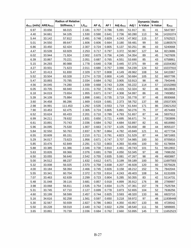
dPCC (mils) AREAPCC

Radius of Relative Stiffness, l L/lest AF do AF l Adj dPCC Adj l

Dynamic k-Value

Static k-Value EPCC

6.97 33.656 66.015 2.181 0.707 0.786 5.091 51.917 81 41 5647397 4.40 34.661 94.105 1.530 0.590 0.641 2.736 60.280 113 56 14191074 5.44 33.142 57.812 2.491 0.748 0.829 4.243 47.902 115 57 5762522 5.01 34.550 89.647 1.606 0.606 0.664 3.180 59.481 99 50 11883576 6.86 33.450 62.424 2.307 0.724 0.805 5.137 50.251 86 43 5240668 4.47 33.539 63.929 2.253 0.717 0.797 3.372 50.967 127 64 8213686 6.02 33.944 71.924 2.002 0.679 0.756 4.245 54.354 89 45 7427609 6.39 33.867 70.221 2.051 0.687 0.765 4.551 53.690 85 43 6758861 5.15 34.293 80.988 1.778 0.640 0.708 3.445 57.375 99 49 10204382 4.27 33.931 71.623 2.011 0.680 0.757 3.066 54.239 124 62 10237910 5.47 33.413 61.830 2.329 0.727 0.808 4.149 49.962 108 54 6413367 5.52 33.504 63.328 2.274 0.720 0.800 4.145 50.684 105 52 6607799 5.47 33.893 70.785 2.034 0.684 0.762 3.905 53.913 98 49 7943446 4.56 34.045 74.280 1.939 0.668 0.743 3.206 55.222 114 57 10152860 6.05 33.705 66.940 2.151 0.702 0.782 4.415 52.324 92 46 6613848 6.18 34.019 73.654 1.955 0.671 0.747 4.308 54.997 86 43 7493852 5.39 34.109 75.884 1.898 0.661 0.735 3.719 55.778 97 48 8930668 3.60 34.458 86.286 1.669 0.619 0.681 2.373 58.752 137 68 15537305 2.98 34.991 111.453 1.292 0.535 0.553 1.719 61.644 171 86 23621202 7.90 33.453 62.475 2.305 0.724 0.805 5.891 50.276 75 37 4574469 6.52 33.624 65.433 2.201 0.710 0.789 4.793 51.657 87 44 5937512 6.99 34.211 78.632 1.831 0.650 0.721 4.695 56.671 74 37 7303899 6.61 33.891 70.743 2.036 0.684 0.762 4.684 53.897 82 41 6616960 5.96 34.095 75.530 1.907 0.663 0.737 4.105 55.658 88 44 8055107 5.84 32.550 50.763 2.837 0.787 0.864 4.782 43.849 121 61 4277734 6.55 33.609 65.151 2.210 0.711 0.791 4.823 51.529 87 44 5871683 5.29 34.017 73.623 1.956 0.671 0.747 3.707 54.985 100 50 8705810 5.85 33.476 62.849 2.291 0.722 0.803 4.393 50.456 100 50 6178694 5.88 33.385 61.386 2.346 0.730 0.810 4.461 49.743 101 51 5912802 5.63 33.826 69.366 2.076 0.691 0.769 4.050 53.345 97 48 7496150 6.50 33.055 56.640 2.542 0.755 0.835 5.081 47.267 98 49 4683887 5.00 34.512 88.237 1.632 0.612 0.671 3.199 59.189 100 50 11697593 5.32 33.008 56.025 2.570 0.758 0.838 4.207 46.928 120 60 5575628 4.00 33.184 58.394 2.466 0.745 0.826 3.158 48.212 152 76 7842044 5.55 33.341 60.704 2.372 0.733 0.814 4.243 49.403 108 54 6131009 7.07 33.463 62.639 2.299 0.723 0.804 5.285 50.355 83 42 5114731 5.48 31.048 39.116 3.681 0.857 0.918 4.899 35.912 176 88 2789997 3.98 33.068 56.811 2.535 0.754 0.834 3.175 47.361 157 78 7525784 5.31 33.745 67.710 2.127 0.699 0.778 3.873 52.655 104 52 7636256 4.60 33.199 58.599 2.457 0.744 0.825 3.593 48.320 133 66 6923710 5.16 34.616 92.258 1.561 0.597 0.650 3.218 59.972 97 48 11938448 5.30 32.567 50.939 2.827 0.786 0.863 4.350 43.957 133 66 4726542 5.50 33.228 59.019 2.440 0.742 0.822 4.256 48.540 111 56 5898665 3.65 33.891 70.739 2.036 0.684 0.762 2.660 53.895 145 72 11652523

B-27

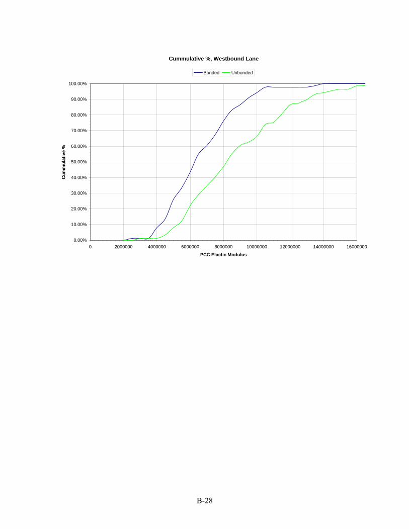
Cummulative %, Westbound Lane

Bonded Unbonded

0 2000000 4000000 6000000 8000000 10000000 12000000 14000000 16000000

PCC Elactic Modulus

0.00%

10.00%

20.00%

30.00%

40.00%

50.00%

60.00%

70.00%

80.00%

90.00%

100.00%

Cum

mul

ativ

e %

B-28

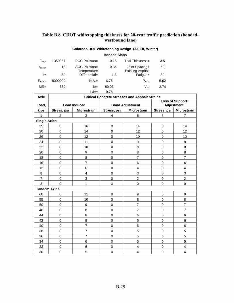
Table B.8. CDOT whitetopping thickness for 20-year traffic prediction (bonded– westbound lane)

Colorado DOT Whitetopping Design (AI, Eff, Winter)

Bonded Slabs

EAC= 1359867 PCC Poisson= 0.15 Trial Thickness= 3.5

tBase= 18 ACC Poisson= 0.35 Joint Spacing= 60 Temperature Existing Asphalt

k= 59 Differential= 1.3 Fatigue= 30

EPCC= 8000000 N.A.= 6.76 PAC= 5.62

MR= 650 le= 80.03 VV= 2.74 L/le= 0.75

Axle

Load, kips

Critical Concrete Stresses and Asphalt Strains

Load Induced Bond Adjustment Loss of Support

Adjustment Stress, psi Microstrain Stress, psi Microstrain Stress, psi Microstrain

1 2 3 4 5 6 7 Single Axles

35 0 16 0 14 0 14 30 0 14 0 12 0 12 26 0 12 0 10 0 10 24 0 11 0 9 0 9 22 0 10 0 8 0 8 20 0 9 0 8 0 8 18 0 8 0 7 0 7 16 0 7 0 6 0 6 12 0 6 0 4 0 4 8 0 4 0 3 0 3 7 0 3 0 2 0 2 3 0 1 0 0 0 0

Tandem Axles 60 0 11 0 9 0 9 55 0 10 0 8 0 8 50 0 9 0 7 0 7 46 0 8 0 7 0 7 44 0 8 0 6 0 6 42 0 8 0 6 0 6 40 0 7 0 6 0 6 38 0 7 0 5 0 5 36 0 7 0 5 0 5 34 0 6 0 5 0 5 32 0 6 0 4 0 4 30 0 5 0 4 0 4

B-29

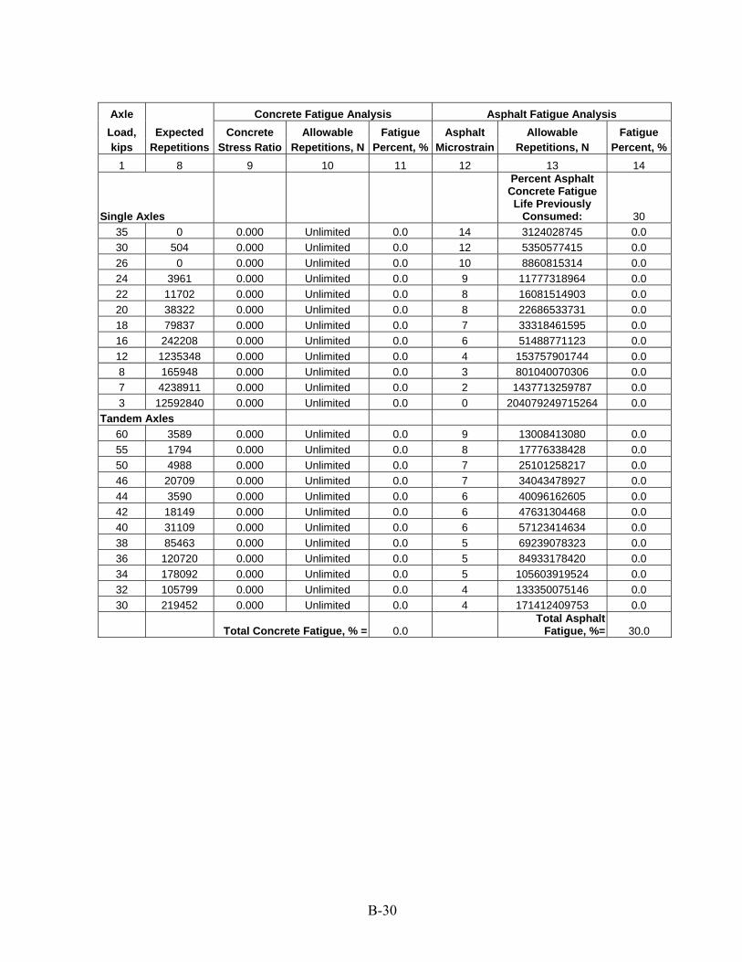
Axle Concrete Fatigue Analysis Asphalt Fatigue Analysis Load, kips

Expected Repetitions

Concrete Stress Ratio

Allowable Repetitions, N

Fatigue Percent, %

Asphalt Microstrain

Allowable Repetitions, N

Fatigue Percent, %

1 8 9 10 11 12 13 14

Single Axles

Percent Asphalt Concrete Fatigue Life Previously

Consumed: 30 35 0 0.000 Unlimited 0.0 14 3124028745 0.0 30 504 0.000 Unlimited 0.0 12 5350577415 0.0 26 0 0.000 Unlimited 0.0 10 8860815314 0.0 24 3961 0.000 Unlimited 0.0 9 11777318964 0.0 22 11702 0.000 Unlimited 0.0 8 16081514903 0.0 20 38322 0.000 Unlimited 0.0 8 22686533731 0.0 18 79837 0.000 Unlimited 0.0 7 33318461595 0.0 16 242208 0.000 Unlimited 0.0 6 51488771123 0.0 12 1235348 0.000 Unlimited 0.0 4 153757901744 0.0 8 165948 0.000 Unlimited 0.0 3 801040070306 0.0 7 4238911 0.000 Unlimited 0.0 2 1437713259787 0.0 3 12592840 0.000 Unlimited 0.0 0 204079249715264 0.0

Tandem Axles 60 3589 0.000 Unlimited 0.0 9 13008413080 0.0 55 1794 0.000 Unlimited 0.0 8 17776338428 0.0 50 4988 0.000 Unlimited 0.0 7 25101258217 0.0 46 20709 0.000 Unlimited 0.0 7 34043478927 0.0 44 3590 0.000 Unlimited 0.0 6 40096162605 0.0 42 18149 0.000 Unlimited 0.0 6 47631304468 0.0 40 31109 0.000 Unlimited 0.0 6 57123414634 0.0 38 85463 0.000 Unlimited 0.0 5 69239078323 0.0 36 120720 0.000 Unlimited 0.0 5 84933178420 0.0 34 178092 0.000 Unlimited 0.0 5 105603919524 0.0 32 105799 0.000 Unlimited 0.0 4 133350075146 0.0 30 219452 0.000 Unlimited 0.0 4 171412409753 0.0

Total Concrete Fatigue, % = 0.0 Total Asphalt

Fatigue, %= 30.0

B-30

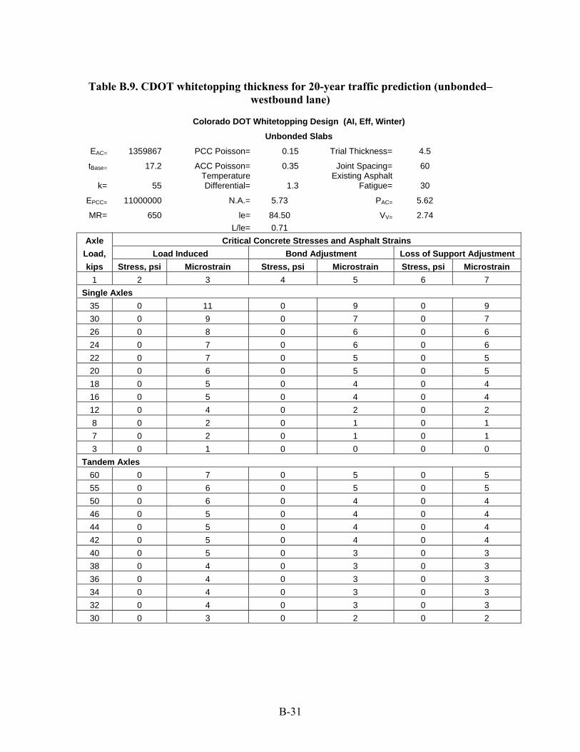
Table B.9. CDOT whitetopping thickness for 20-year traffic prediction (unbonded– westbound lane)

Colorado DOT Whitetopping Design (AI, Eff, Winter)

Unbonded Slabs

EAC= 1359867 PCC Poisson= 0.15 Trial Thickness= 4.5

tBase= 17.2 ACC Poisson= 0.35 Joint Spacing= 60 Temperature Existing Asphalt

k= 55 Differential= 1.3 Fatigue= 30

EPCC= 11000000 N.A.= 5.73 PAC= 5.62

MR= 650 le= 84.50 VV= 2.74 L/le= 0.71

Axle Load, kips

Critical Concrete Stresses and Asphalt Strains Load Induced Bond Adjustment Loss of Support Adjustment

Stress, psi Microstrain Stress, psi Microstrain Stress, psi Microstrain 1 2 3 4 5 6 7

Single Axles 35 0 11 0 9 0 9 30 0 9 0 7 0 7 26 0 8 0 6 0 6 24 0 7 0 6 0 6 22 0 7 0 5 0 5 20 0 6 0 5 0 5 18 0 5 0 4 0 4 16 0 5 0 4 0 4 12 0 4 0 2 0 2 8 0 2 0 1 0 1 7 0 2 0 1 0 1 3 0 1 0 0 0 0

Tandem Axles 60 0 7 0 5 0 5 55 0 6 0 5 0 5 50 0 6 0 4 0 4 46 0 5 0 4 0 4 44 0 5 0 4 0 4 42 0 5 0 4 0 4 40 0 5 0 3 0 3 38 0 4 0 3 0 3 36 0 4 0 3 0 3 34 0 4 0 3 0 3 32 0 4 0 3 0 3 30 0 3 0 2 0 2

B-31

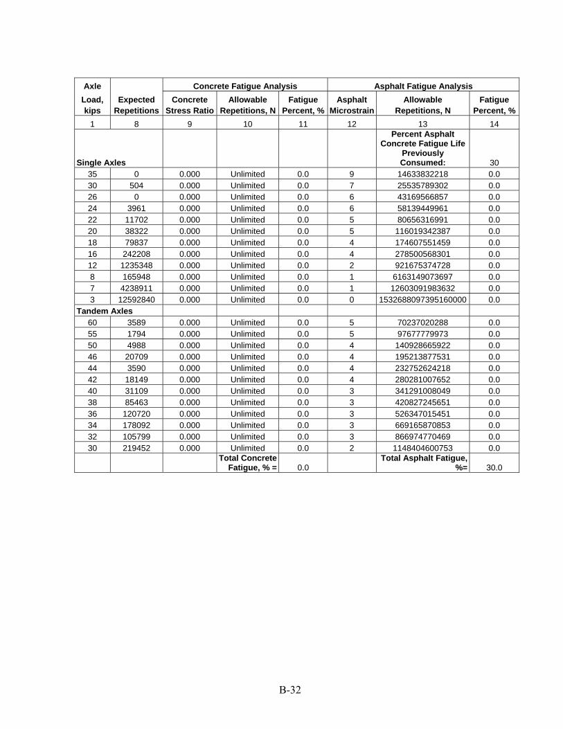
Axle Concrete Fatigue Analysis Asphalt Fatigue Analysis Load, kips

Expected Repetitions

Concrete Stress Ratio

Allowable Repetitions, N

Fatigue Percent, %

Asphalt Microstrain

Allowable Repetitions, N

Fatigue Percent, %

1 8 9 10 11 12 13 14

Single Axles

Percent Asphalt Concrete Fatigue Life

Previously Consumed: 30

35 0 0.000 Unlimited 0.0 9 14633832218 0.0 30 504 0.000 Unlimited 0.0 7 25535789302 0.0 26 0 0.000 Unlimited 0.0 6 43169566857 0.0 24 3961 0.000 Unlimited 0.0 6 58139449961 0.0 22 11702 0.000 Unlimited 0.0 5 80656316991 0.0 20 38322 0.000 Unlimited 0.0 5 116019342387 0.0 18 79837 0.000 Unlimited 0.0 4 174607551459 0.0 16 242208 0.000 Unlimited 0.0 4 278500568301 0.0 12 1235348 0.000 Unlimited 0.0 2 921675374728 0.0 8 165948 0.000 Unlimited 0.0 1 6163149073697 0.0 7 4238911 0.000 Unlimited 0.0 1 12603091983632 0.0 3 12592840 0.000 Unlimited 0.0 0 1532688097395160000 0.0

Tandem Axles 60 3589 0.000 Unlimited 0.0 5 70237020288 0.0 55 1794 0.000 Unlimited 0.0 5 97677779973 0.0 50 4988 0.000 Unlimited 0.0 4 140928665922 0.0 46 20709 0.000 Unlimited 0.0 4 195213877531 0.0 44 3590 0.000 Unlimited 0.0 4 232752624218 0.0 42 18149 0.000 Unlimited 0.0 4 280281007652 0.0 40 31109 0.000 Unlimited 0.0 3 341291008049 0.0 38 85463 0.000 Unlimited 0.0 3 420827245651 0.0 36 120720 0.000 Unlimited 0.0 3 526347015451 0.0 34 178092 0.000 Unlimited 0.0 3 669165870853 0.0 32 105799 0.000 Unlimited 0.0 3 866974770469 0.0 30 219452 0.000 Unlimited 0.0 2 1148404600753 0.0

Total Concrete Fatigue, % = 0.0

Total Asphalt Fatigue, %= 30.0

B-32

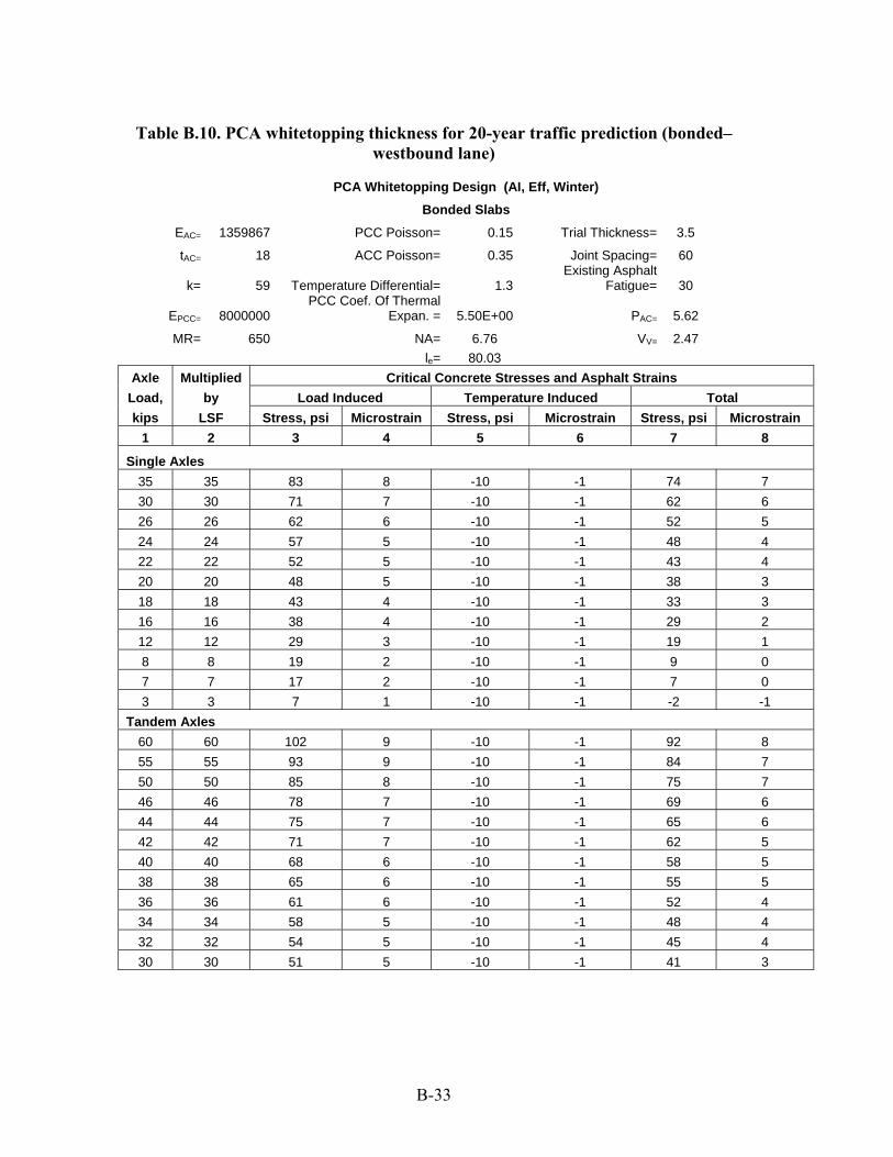
Table B.10. PCA whitetopping thickness for 20-year traffic prediction (bonded– westbound lane)

PCA Whitetopping Design (AI, Eff, Winter)

Bonded Slabs

EAC= 1359867 PCC Poisson= 0.15 Trial Thickness= 3.5

tAC= 18 ACC Poisson= 0.35 Joint Spacing= 60 Existing Asphalt

k= 59 Temperature Differential= 1.3 Fatigue= 30 PCC Coef. Of Thermal

EPCC= 8000000 Expan. = 5.50E+00 PAC= 5.62

MR= 650 NA= 6.76 VV= 2.47 le = 80.03

AxleLoad, kips

Multiplied by

LSF

Critical Concrete Stresses and Asphalt Strains Load Induced Temperature Induced Total

Stress, psi Microstrain Stress, psi Microstrain Stress, psi Microstrain 1 2 3 4 5 6 7 8

Single Axles 35 35 83 8 -10 -1 74 7 30 30 71 7 -10 -1 62 6 26 26 62 6 -10 -1 52 5 24 24 57 5 -10 -1 48 4 22 22 52 5 -10 -1 43 4 20 20 48 5 -10 -1 38 3 18 18 43 4 -10 -1 33 3 16 16 38 4 -10 -1 29 2 12 12 29 3 -10 -1 19 1 8 8 19 2 -10 -1 9 0 7 7 17 2 -10 -1 7 0 3 3 7 1 -10 -1 -2 -1

Tandem Axles 60 60 102 9 -10 -1 92 8 55 55 93 9 -10 -1 84 7 50 50 85 8 -10 -1 75 7 46 46 78 7 -10 -1 69 6 44 44 75 7 -10 -1 65 6 42 42 71 7 -10 -1 62 5 40 40 68 6 -10 -1 58 5 38 38 65 6 -10 -1 55 5 36 36 61 6 -10 -1 52 4 34 34 58 5 -10 -1 48 4 32 32 54 5 -10 -1 45 4 30 30 51 5 -10 -1 41 3

B-33

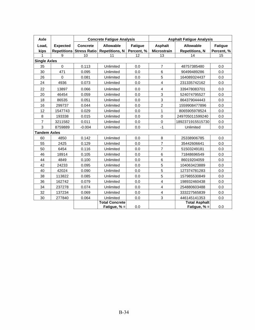
Axle Load, kips

Expected Repetitions

Concrete Fatigue Analysis Asphalt Fatigue Analysis Concrete

Stress Ratio Allowable

Repetitions, N Fatigue

Percent, % Asphalt

Microstrain Allowable

Repetitions, N Fatigue

Percent, % 1 9 10 11 12 13 14 15

Single Axles 35 0 0.113 Unlimited 0.0 7 48757385480 0.0 30 471 0.095 Unlimited 0.0 6 90499489286 0.0 26 0 0.081 Unlimited 0.0 5 164089324437 0.0 24 4936 0.073 Unlimited 0.0 4 231335742162 0.0

22 13897 0.066 Unlimited 0.0 4 339478083701 0.0 20 46454 0.059 Unlimited 0.0 3 524074795527 0.0 18 86535 0.051 Unlimited 0.0 3 864379044443 0.0 16 299737 0.044 Unlimited 0.0 2 1559908477896 0.0 12 1547743 0.029 Unlimited 0.0 1 8065905978524 0.0 8 193338 0.015 Unlimited 0.0 0 249705011599240 0.0 7 3211582 0.011 Unlimited 0.0 0 1892371915515730 0.0 3 8759889 -0.004 Unlimited 0.0 -1 Unlimited 0.0

Tandem Axles 60 4850 0.142 Unlimited 0.0 8 25338906785 0.0 55 2425 0.129 Unlimited 0.0 7 35442606641 0.0 50 6454 0.116 Unlimited 0.0 7 51503249181 0.0 46 18914 0.105 Unlimited 0.0 6 71848696549 0.0 44 4849 0.100 Unlimited 0.0 6 86019204059 0.0 42 24233 0.095 Unlimited 0.0 5 104063423889 0.0 40 42024 0.090 Unlimited 0.0 5 127374781283 0.0 38 113822 0.085 Unlimited 0.0 5 157985530849 0.0 36 162742 0.079 Unlimited 0.0 4 198932460438 0.0 34 237278 0.074 Unlimited 0.0 4 254880603488 0.0 32 137234 0.069 Unlimited 0.0 4 333227565839 0.0 30 277840 0.064 Unlimited 0.0 3 446145141353 0.0

Total Concrete Fatigue, % = 0.0

Total Asphalt Fatigue, % = 0.0

B-34

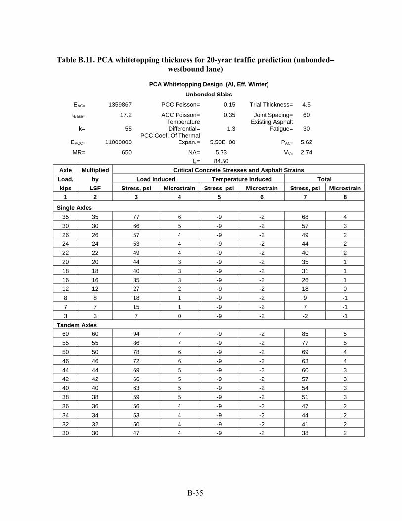
Table B.11. PCA whitetopping thickness for 20-year traffic prediction (unbonded– westbound lane)

PCA Whitetopping Design (AI, Eff, Winter)

Unbonded Slabs

EAC= 1359867 PCC Poisson= 0.15 Trial Thickness= 4.5

tBase= 17.2 ACC Poisson= 0.35 Joint Spacing= 60 Temperature Existing Asphalt

k= 55 Differential= 1.3 Fatigue= 30 PCC Coef. Of Thermal

EPCC= 11000000 Expan.= 5.50E+00 PAC= 5.62

MR= 650 NA= 5.73 VV= 2.74 le = 84.50

AxleLoad, kips

Multiplied by

LSF

Critical Concrete Stresses and Asphalt Strains Load Induced Temperature Induced Total

Stress, psi Microstrain Stress, psi Microstrain Stress, psi Microstrain 1 2 3 4 5 6 7 8

Single Axles 35 35 77 6 -9 -2 68 4 30 30 66 5 -9 -2 57 3 26 26 57 4 -9 -2 49 2 24 24 53 4 -9 -2 44 2 22 22 49 4 -9 -2 40 2 20 20 44 3 -9 -2 35 1 18 18 40 3 -9 -2 31 1 16 16 35 3 -9 -2 26 1 12 12 27 2 -9 -2 18 0 8 8 18 1 -9 -2 9 -1 7 7 15 1 -9 -2 7 -1 3 3 7 0 -9 -2 -2 -1

Tandem Axles 60 60 94 7 -9 -2 85 5 55 55 86 7 -9 -2 77 5 50 50 78 6 -9 -2 69 4 46 46 72 6 -9 -2 63 4 44 44 69 5 -9 -2 60 3 42 42 66 5 -9 -2 57 3 40 40 63 5 -9 -2 54 3 38 38 59 5 -9 -2 51 3 36 36 56 4 -9 -2 47 2 34 34 53 4 -9 -2 44 2 32 32 50 4 -9 -2 41 2 30 30 47 4 -9 -2 38 2

B-35

Axle Load, kips

Expected Repetitions

Concrete Fatigue Analysis Asphalt Fatigue Analysis Concrete

Stress Ratio Allowable

Repetitions, N Fatigue

Percent, % Asphalt

Microstrain Allowable

Repetitions, N Fatigue

Percent, % 1 9 10 11 12 13 14 15

Single Axles 35 0 0.105 Unlimited 0.0 4 318114132260 0.0 30 471 0.088 Unlimited 0.0 3 712946565378 0.0 26 0 0.075 Unlimited 0.0 2 1630994471997 0.0 24 4936 0.068 Unlimited 0.0 2 2709818003389 0.0

22 13897 0.061 Unlimited 0.0 2 4940515459044 0.0 20 46454 0.054 Unlimited 0.0 1 10306117833832 0.0 18 86535 0.047 Unlimited 0.0 1 26604723481723 0.0 16 299737 0.041 Unlimited 0.0 1 101374982690248 0.0 12 1547743 0.027 Unlimited 0.0 0 Unlimited 0.0 8 193338 0.014 Unlimited 0.0 -1 Unlimited 0.0 7 3211582 0.010 Unlimited 0.0 -1 Unlimited 0.0 3 8759889 -0.003 Unlimited 0.0 -1 Unlimited 0.0

Tandem Axles 60 4850 0.131 Unlimited 0.0 5 105731872607 0.0 55 2425 0.119 Unlimited 0.0 5 157742070969 0.0 50 6454 0.107 Unlimited 0.0 4 248758902666 0.0 46 18914 0.097 Unlimited 0.0 4 377123569121 0.0 44 4849 0.092 Unlimited 0.0 3 474458486341 0.0 42 24233 0.087 Unlimited 0.0 3 607291477740 0.0 40 42024 0.083 Unlimited 0.0 3 793041579438 0.0 38 113822 0.078 Unlimited 0.0 3 1060308707898 0.0 36 162742 0.073 Unlimited 0.0 2 1458114757734 0.0 34 237278 0.068 Unlimited 0.0 2 2074912003885 0.0 32 137234 0.063 Unlimited 0.0 2 3080567886888 0.0 30 277840 0.059 Unlimited 0.0 2 4827576637260 0.0

Total Concrete Fatigue, % = 0.0

Total Asphalt Fatigue, % = 0.0

B-36