Embed Size (px)
Citation preview
International Journal of Scientific Engineering and Research (IJSER) www.ijser.in
ISSN (Online): 2347-3878, Impact Factor (2015): 3.791
Volume 4 Issue 6, June 2016 Licensed Under Creative Commons Attribution CC BY
Design and Comparison of Different Controllers to
Stabilize a Rotary Inverted Pendulum
Kambhampati Tejaswi1, Alluri Amarendra
2, Ganta Ramesh
3
1M.Tech, Department of EEE, Gudlavalleru engineering college, Gudlavalleru, Krishna [A.P], India
2Associate professor, Department of EEE, Gudlavalleru engineering college, Gudlavalleru, Krishna [A.P], India 3Assistant professor, Department of EEE, Gudlavalleru engineering college, Gudlavalleru, Krishna [A.P], India
Abstract: This paper describes the design procedures and design of various controllers for stabilizing a Rotary Inverted Pendulum
System (RIPS). A PV (Position-Velocity) controller, LQR (Linear Quadratic Regulator) controller with different weighing matrices and
an observer-based controller are tried on RIPS in MATLAB Simulink. The outputs obtained with different weighing matrices are
observed and compared for different conclusions. The controllers with the best values obtained in the simulation are tested on a test-bed
of RIPS and are compared for various aspects. The controllers in Simulink are compared with the controllers in real time.
Keywords: Rotary Inverted Pendulum, PV, LQR, Weighing Matrices, Observer-Based control
1.Introduction
A typical unstable non-linear Inverted Pendulum system is
often used as a benchmark to study various control
techniques in control engineering. Analysis of controllers
on RIP illustrates the analysis in cases such as control of a
space booster rocket and a satellite, an automatic aircraft
landing system, aircraft stabilization in the turbulent air-
flow, stabilization of a cabin in a ship etc. RIP is a test bed
for the study of various controllers like PID controller,
LQR controller, Robust controllers, Fuzzy-Logic, AI
techniques, GA techniques and any more. A normal
pendulum is stable when hanging downwards, an inverted
pendulum is inherently unstable, and must be actively
balanced in order to remain upright, this can be done by
applying a torque at the pivot point, by moving the pivot
point horizontally as part of a feedback system.
In this paper controllers are developed that keep the
pendulum upright without any oscillations. The model is
simulated using the MATLAB application. The paper is
organized as follows. Section 2 deals with the modelling
of the system, Section 3 discusses the control techniques
PID, LQR, observer based controller, Section 4 gives the
test bed results, and Section 5 discusses the conclusion
drawn from the analysis of these controllers in Simulink
and on test bed.
2.Modelling of Rotary Inverted Pendulum
The Rotary Inverted Pendulum mainly consists of a rotary
arm, vertical pendulum, and a servo motor which drives
the system. An encoder is attached to the arm shaft in
order to measure the rotation angle of the arm and
pendulum.
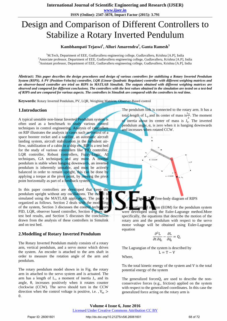
The rotary pendulum model shown in in Fig. the rotary
arm in attached to the servo system and is actuated. The
arm has a length of Lr, a moment of inertia Jr, and its
angle, θ, increases positively when it rotates counter
clockwise (CCW). The servo should turn in the CCW
direction when the control voltage is positive, i.e. , Vm >0.
The pendulum link is connected to the rotary arm. It has a
total length of Lp and its center of mass isLp
2. The moment
of inertia about its center of mass is Jp. The inverted
pendulum angle, α, is zero when it is hanging downwards
and increases when rotated CCW.
Figure 2.1: Free-body diagram of RIPS
The equations of motion (EOM) for the pendulum system
were developed using the Euler-Lagrange method.More
specifically, the equations that describe the motion of the
rotary arm and the pendulum with respect to the servo
motor voltage will be obtained using Euler-Lagrange
equation
∂2L
∂t ∂q i−
∂L
∂q i= Qi
The Lagrangian of the system is described by
L = T − V
Where,
Tis the total kinetic energy of the system and V is the total
potential energy of the system
The generalized forcesQi are used to describe the non-
conservative forces (e.g., friction) applied on the system
with respect to the generalized coordinates. In this case the
generalized force acting on the rotary arm is
Paper ID: 26061601 http://dx.doi.org/10.21275/v5i6.26061601 68 of 72

International Journal of Scientific Engineering and Research (IJSER) www.ijser.in
ISSN (Online): 2347-3878, Impact Factor (2015): 3.791
Volume 4 Issue 6, June 2016 Licensed Under Creative Commons Attribution CC BY
Q1 = τ − Drθ
and acting on the pendulum is
Q2 = −Dpα
The total potential energy of the system is
V = mgLp
2cos(α)
and the total kinetic energy of the system is
T =1
2 Jr + mpLr
2 θ 2 +2
3mpLp
2α 2 − mpLpLrcos α θ α
Solving the above two equations for the Lagrangian and
the derivatives, the EOM of the system are
mpLr2 +
1
4mpLp
2 −1
4mpLp
2cos2 α + Jr θ − 1
2mpLpLr cos α α +
1
2mpLp
2 sin α cos α θ α
+ 1
2mpLpLr sin α α 2 = τ − Drθ
1
2mpLrLp cos α θ + Jp +
1
4mpLp
2 α −1
4mpLp
2 cos α sin α θ 2 +1
2mpLpg sin α = −Dpα
The torque applied at the base of the rotary arm is described as
τ =ηgηm kgktkm (Vm − kmθ)
Rm
When the nonlinear equations are linearized about the operating point θ, α = (0,0), the resultant EMO of the inverted
pendulum are defined as:
mpLr2 + Jr θ −
1
2mpLpLrα = τ − Drθ
and
1
2𝑚𝑝𝐿𝑟𝐿𝑝𝜃 + 𝐽𝑝 +
1
4𝑚𝑝𝐿𝑝
2 𝛼 +1
2𝑚𝑝𝐿𝑝𝑔𝛼 = −𝐷𝑝𝛼
Solving the above equations for the acceleration terms yields
𝜃 =1
𝐽𝑇 − 𝐽𝑝 +
1
4𝑚𝑝𝐿𝑝
2 𝐷𝑟𝜃 +1
2𝑚𝑝𝐿𝑝𝐿𝑟𝐷𝑝𝛼 +
1
4𝑚𝑝
2𝐿𝑝2𝐿𝑟𝑔𝛼 + 𝐽𝑝 +
1
4𝑚𝑝𝐿𝑝
2 𝜏
and
𝛼 =1
𝐽𝑇 1
2𝑚𝑝𝐿𝑝𝐿𝑟𝐷𝑟𝜃 − 𝐽𝑟 + 𝑚𝑝𝐿𝑟
2 𝐷𝑝𝛼 −1
2𝑚𝑝𝐿𝑝𝑔 𝐽𝑟 + 𝑚𝑝𝐿𝑟
2 𝛼 −1
2𝑚𝑝𝐿𝑝𝐿𝑟𝜏
Where
𝐽𝑇 = 𝐽𝑝𝑚𝑝𝐿𝑟2 + 𝐽𝑟𝐽𝑝 +
1
4𝐽𝑟𝑚𝑝𝐿𝑝
2
The A and B matrices for state-space representation can then be found as
𝐴 =1
𝐽𝑇
0 0 1 00 0 0 1
01
4𝑚𝑝
2𝐿𝑝2𝐿𝑟𝑔 − 𝐽𝑝 +
1
4𝑚𝑝𝐿𝑝
2 𝐷𝑟
1
2𝑚𝑝𝐿𝑝𝐿𝑟𝐷𝑝
0 −1
2𝑚𝑝𝐿𝑝𝑔 𝐽𝑟 + 𝑚𝑝𝐿𝑟
2 1
2𝑚𝑝𝐿𝑝𝐿𝑟𝐷𝑟 − 𝐽𝑟 + 𝑚𝑝𝐿𝑟
2 𝐷𝑝
𝐵 =1
𝐽𝑇
00
𝐽𝑝 +1
4𝑚𝑝𝐿𝑝
2
−1
2𝑚𝑝𝐿𝑝𝐿𝑟
Paper ID: 26061601 http://dx.doi.org/10.21275/v5i6.26061601 69 of 72

International Journal of Scientific Engineering and Research (IJSER) www.ijser.in
ISSN (Online): 2347-3878, Impact Factor (2015): 3.791
Volume 4 Issue 6, June 2016 Licensed Under Creative Commons Attribution CC BY
3.Design of Controllers for Rotary Inverted
Pendulum
3.1 PV (Position-velocity) Control
In this paper we will find control strategies that balance
the pendulum in the upright position while maintaining a
desired position of the arm. When balancing the system,
the pendulum angle 𝛼 is small and balancing can be
accomplished with a simple PD controller, as shown in
Figure 3.1.1. The control law can then be expressed as
𝑢 = 𝑘𝑝 ,𝜃 𝜃𝑟 − 𝜃 − 𝑘𝑝 ,𝛼𝛼 − 𝑘𝑑 ,𝜃𝜃 − 𝑘𝑑 ,𝛼𝛼
Where, 𝑘𝑝 ,𝜃 is the arm angle proportional gain, 𝑘𝑝 ,𝛼 is the
pendulum angle proportional gain, 𝑘𝑑 ,𝜃 is the arm angle
derivative gain, 𝑘𝑑 ,𝛼 is the pendulum angle derivative
gain. The desired angle of the arm is denoted by 𝜃𝑟 and
the reference for the pendulum position is zero (i.e.
upright position).
Figure 3.1.1: Block Diagram of PV Controller
As mentioned, the integral term is eliminated taking the
constraints of noise and derivative control is used as a
velocity feedback and only negative velocity is fed-back
to the system. And in practical system we use a filter to
suppress the noise generated by the derivative control. By
trial and error method we obtain the gain values of the
controller as Kd = −2, Kp = 2 for the control of the rotary
arm and Kd = 2.5, Kp = 30 for the control of the
pendulum.
3.2 LQR Controller
Linear Quadratic Regulator (LQR) theory is a technique
that is ideally suited for finding the parameters of the
pendulum balance controller. Given that the equations of
motion of the system can be described in the form
x = Ax + Bu
Where Aand Bare the state and input matrices,
respectively, the LQR algorithm computes a control law u
such that the performance criterion or cost function
J = xref − x t T
Q xref − x t + u t TRu t dt
∞
0
is minimized. The design matrices Q and R hold the
penalties on the deviations of the state variables from their
set-point and the control actions, respectively. When an
element of Q is increased, therefore, the cost function
increases the penalty associated with any deviations from
the desired set-point of that state variable, and thus the
specific control gain will be larger. When the values of the
R matrix are increased, a larger penalty is applied to the
aggressiveness of the control action and the control gains
are uniformly decreased. In our case the state vector x is
defined
x = [θ α θ α ]T
Figure 3.2.1: Block diagram of an LQR Controller
Since there is only one control variable, R is a scalar. The
reference signal xref is set to [θr 0 0 0], and the control
strategy used to minimize cost function J is thus given by
u = K xref − x = kp,θ θr − θ − kp,αα − kd,θθ − kd,αα
This control law is a state-feedback control and is
illustrated in the above figure. It is equivalent to the PV
control designed.
The LQR gain matrix K is obtained by using MATLAB
software, using code “lqr(A,B,Q,R)”.
3.3 Observer-Based control
Figure 3.3.1: Block diagram of observer based control
In LQR, all the states are utilised which is an unnecessary
action. Hence, here in observer control, we use only the
states which are necessary for the control action. To
address the situation where not all the state variables are
measured, a state estimator must be designed. A schematic
of the state estimator is shown below.
The condition to be met is that the system states are
completely observable. The dynamics of the state estimate
is described by the following equation.
x = Ax + Bu + L(y − y )
Paper ID: 26061601 http://dx.doi.org/10.21275/v5i6.26061601 70 of 72

International Journal of Scientific Engineering and Research (IJSER) www.ijser.in
ISSN (Online): 2347-3878, Impact Factor (2015): 3.791
Volume 4 Issue 6, June 2016 Licensed Under Creative Commons Attribution CC BY
The dynamics of the error in the state estimate is described
by
e = x − x = Ax + Bu − (Ax + Bu + L Cx − Cx )
e = A − LC e
Combining the LQR with the state estimate gives us the
full compensator and the state-space matrices are given by
x e =
A − BK BK0 A − LC
xe + BN
0 r
y = C 0 xe + 0 r
4.Simulation & Results
The model parameters are shown in below table.
Table 1: Rotary Inverted pendulum Parameters Motor
Rm = 8.4 Resistance
Kt = 0.042 Current-torque (N-m/A)
Km = 0.042 Back-emf constant (V-s/rad)
Rotary Arm
Mr = 0.095 Mass (kg)
Lr = 0.085 Total length (m)
Jr = Mr*Lr2/12
Moment of inertia about pivot (kg-
m^2)
Dr = 0.0015 Equivalent Viscous Damping
Coefficient (N-m-s/rad)
Pendulum Link
Mp = 0.024 Mass (kg)
Lp = 0.129 Total length (m)
Jp = Mp*Lp2/12
Moment of inertia about pivot (kg-
m^2)
Dp = 0.0005 Equivalent Viscous Damping
Coefficient (N-m-s/rad)
g = 9.81 Gravity Constant
After substituting RIP parameters in A and B matrices, we
can get
A =
0 0 1 00 0 0 10 149.2751 −14.9183 49.14930 −261.6091 14.7448 −86.1356
B =
00
49.7275−49.1493
4.1 PV Controller
Figure 4.1.1: Simulink Model of PV Controller
Figure 4.1.2: Response of arm for a PV Controller
Figure 4.1.3: Response of Pendulum for a PV
4.2 LQR Controller
Figure 4.2.1: Simulink Model of an LQR Controller
For R=1; Q=[20 0 0 0; 0 5 0 0; 0 0 1 0; 0 0 0 1]:
K = [4.4721 1.3528 0.9364 0.4866]
Figure 4.2.2: Response of arm
Figure 4.2.3: Response of pendulum
For R=15, Q=[20 0 0 0; 0 5 0 0; 0 0 1 0; 0 0 0 1]:
K = [1.1547 0.2361 0.2010 0.1185]
Paper ID: 26061601 http://dx.doi.org/10.21275/v5i6.26061601 71 of 72

International Journal of Scientific Engineering and Research (IJSER) www.ijser.in
ISSN (Online): 2347-3878, Impact Factor (2015): 3.791
Volume 4 Issue 6, June 2016 Licensed Under Creative Commons Attribution CC BY
Figure 4.2.4: Response of arm
Figure 4.2.5: Response of pendulum
For R=25, Q=[20 0 0 0;0 5 0 0; 0 0 1 0; 0 0 0 1]:
K = [0.8944 0.1586 0.1499 0.0889]
Figure 4.2.8: Response of arm
Figure 4.2.9: Response of pendulum
4.3 Observer-Based control
Figure 4.3.1: Simulink Model of observer-based control
Figure 4.3.2: Response of Rotary arm
Figure 4.3.3: Response of pendulum
4.4 Comparison of PV and LQR controllers
Figure 4.4.1: Response of Rotary arm
Figure 4.4.2: Response of Pendulum
5.Conclusions
From the simulation results, we can observe that the
system can be stabilized by many controllers. But the
necessity is for the controller with better response. Among
PV and LQR controllers, LQR controller gives much
better response. Using the Observer-based control, we can
minimize the error and neglect the unnecessary states
while controlling. Even though there wouldn’t be any
difference in the output, but coming to the application
oriented it simplifies and reduces the cost required to build
the application.
References
[1] Control Systems Engineering, 6th Edition by Norman
S Nise, John Wiley & Sons Inc., 2011.
[2] Feedback Systems, Electronic Edition 2.11b, K.J.
Astrom, Richard M Murray, Princeton University
Press, 2012.
[3] Feedback Control of Dynamic Systems, 6th Edition,
Gene F Franklin, J Dvaid Powell, Abbas Emai-
Naeini, Pearson Higher Education Inc., 2010.
[4] Modern Control Systems, 12th Edition, Richard C
Dorf, Robert H Bishop, Pearson Higher Education,
2011.
[5] Modern Control Engineering, 5th Edition, Katsuhiko
Ogata, Pearson Education, 2010
[6] Automatic control Systems, 9th Edition, Farid
Golnaraghi, Benajmin C Kuo, John Wiley & Sons
Inc., 2010.
[7] Control Systems Engineering, 5th Edition, I J Nagrath,
M Gopal, Anshan Ltd and New Age International
Ltd, 2008.
[8] Mechatronics, 3rd Edition, W Bolton, Pearson
Education Ltd, 2003
Paper ID: 26061601 http://dx.doi.org/10.21275/v5i6.26061601 72 of 72


![Inverted Pendulum [Final]](https://img.pdfslide.us/doc/110x75/58904db31a28abcb668bcda8/inverted-pendulum-final.jpg)