Embed Size (px)
Citation preview
Rochester Institute of Technology Rochester Institute of Technology
RIT Scholar Works RIT Scholar Works
Theses
5-17-2017
Design and Analysis of Multiple-Load Automated Guided Vehicle Design and Analysis of Multiple-Load Automated Guided Vehicle
Dispatching Algorithms Dispatching Algorithms
Maojia Li [email protected]
Follow this and additional works at: https://scholarworks.rit.edu/theses
Recommended Citation Recommended Citation Li, Maojia, "Design and Analysis of Multiple-Load Automated Guided Vehicle Dispatching Algorithms" (2017). Thesis. Rochester Institute of Technology. Accessed from
This Thesis is brought to you for free and open access by RIT Scholar Works. It has been accepted for inclusion in Theses by an authorized administrator of RIT Scholar Works. For more information, please contact [email protected].
DESIGN AND ANALYSIS OF MULTIPLE-LOAD AUTOMATED
GUIDED VEHICLE DISPATCHING ALGORITHMS
By
Maojia Li
A Thesis Submitted in Partial Fulfilment of the Requirement
for the Degree of Master of Science in
Manufacturing and Mechanical Systems Integration
Department of Manufacturing and Mechanical Engineering Technology
College of Applied Science and Technology
Rochester Institute of Technology
Rochester, NY
May 17, 2017

i
ACKNOWLEDGMENTS
I take this opportunity to express my sincere gratitude to my thesis advisor Dr. Michael Kuhl for his
exemplary guidance, patience, and encouragement through this thesis. Dr. Kuhl dedicated his valuable time
to guide my research and review my work constantly. His support has enabled me to complete this thesis.
I also thank my thesis committee members Dr. Manian Ramkumar and Dr. James Lee who provided me
support and valuable suggestions. I would like to extend my sincerest thanks to my parents, Mr. Chunbin
Li and Mrs. Jing Zou for supporting me from the beginning of my lifetime.
ii
ABSTRACT
This paper addresses the problems of dispatching multiple-load automated guided vehicles
(AGVs) in flexible manufacturing systems (FMSs). A pickup-or-delivery-en-route (PDER) rule is
proposed to address the task-determination problem that indicates if a partially loaded AGV’s next
task should be picking up a new job or dropping off a carried load. A workload-balancing (WLB)
algorithm is developed to deal with the pickup-dispatching problem that determines which job
should be assigned to an AGV. A simulation experiment is conducted to compare the PDER rule
with an existing task-determination rule in 2 representative FMSs. We use another simulation
experiment to compare the WLB rule with 4 existing pickup-dispatching rules in 3 FMSs. The
results show that the PDER rule can significantly improve the system throughput and reduce the
average time in system of parts, while the WLB rule also has an outstanding throughput
performance.
iii
Table of Contents
ACKNOWLEDGMENTS ........................................................................................................................... i
ABSTRACT ................................................................................................................................................. ii
Table of Contents ....................................................................................................................................... iii
List of Tables ............................................................................................................................................... v
List of Figures ............................................................................................................................................. vi
Notation ..................................................................................................................................................... viii
1. INTRODUCTION ................................................................................................................................... 1
2. PROBLEM STATEMENT .................................................................................................................... 3
3. LITERATURE REVIEW ...................................................................................................................... 4
3.1 Scheduling vs. Dispatching ............................................................................................................... 4
3.2 Multiple-load AGV Dispatching ...................................................................................................... 4
3.3 Workcenter-initiated vs. Vehicle-initiated Dispatching Rules ...................................................... 6
3.4 Multi-attributed vs. Hierarchical Dispatching Algorithms ........................................................... 8
3.5 Discussion........................................................................................................................................... 8
4. ALGORITHM DESIGN ...................................................................................................................... 12
4.1 Pickup-or-Delivery-En-Route Rule ............................................................................................... 12
4.1.1 Important Queues ....................................................................................................................... 12
4.1.2 Flowchart ................................................................................................................................... 13
4.1.3 Example of PDER Rule .............................................................................................................. 15
4.2 Workload Balancing Rule .................................................................................................................. 17
4.2.1 Workload Balancing Concept .................................................................................................... 17
4.2.2 Job Evaluation ........................................................................................................................... 18
4.2.3 Example of WLB Algorithm ....................................................................................................... 18
4.3 AGV Control Rules ......................................................................................................................... 19
4.3.1 Workcenter-initiated Rule .......................................................................................................... 19
4.3.2 Delivery-dispatching Rule .......................................................................................................... 19
4.3.3 Load-selection Rule.................................................................................................................... 19
4.3.4 Pickup-dispatching Rules ........................................................................................................... 20
4.3.5 Task-determination Rule ............................................................................................................ 20
5. IMPLEMENTATION .......................................................................................................................... 22
5.1 Implementation of PDER ............................................................................................................... 22
5.2 Implementation of DTF .................................................................................................................. 26
iv
5.3 Implementation of WLB ................................................................................................................. 27
6. EXPERIMENT FOR THE PDER RULE ........................................................................................... 29
6.1 Experiment Design (Experiment 1) ............................................................................................... 29
6.1.1 FMS 1 Configuration (Experiment 1) ........................................................................................ 29
6.1.2 FMS 2 Configuration (Experiment 1) ........................................................................................ 30
6.2 Output Analysis (Experiment 1) .................................................................................................... 32
7. EXPERIMENT FOR THE PDER AND WLB RULES..................................................................... 36
7.1 Experiment Design (Experiment 2) ............................................................................................... 36
7.1.1 FMS 1 Configuration (Experiment 2) ........................................................................................ 36
7.1.2 FMS 2 Configuration (Experiment 2) ........................................................................................ 37
7.1.3 FMS 3 Configuration (Experiment 2) ........................................................................................ 37
7.2 Output Analysis (Experiment 2) .................................................................................................... 38
7.2.1 FMS 1 Output Analysis (Experiment 2) ..................................................................................... 40
7.2.2 FMS 2 Output Analysis (Experiment 2) ..................................................................................... 43
7.2.3 FMS 3 Output Analysis (Experiment 2) ..................................................................................... 47
8. MAJOR FINDINGS ............................................................................................................................. 51
9. CONCLUSION ..................................................................................................................................... 54
REFERENCES .......................................................................................................................................... 55
APPENDIX ................................................................................................................................................ 57
Simio Processes...................................................................................................................................... 57
Throughput Analysis ............................................................................................................................ 60
AGV Capacity Utilization Analysis ..................................................................................................... 62
v
List of Tables
Table 1: Differences in vehicle states between single- and dual-load AGVs. ............................................ 12
Table 2: Factors considered in experiment 1. ............................................................................................. 29
Table 3: Part routing and processing information for FMS 1, experiment 1. ............................................. 30
Table 4: Part routing and production volume percentages for FMS 2. ....................................................... 31
Table 5: Processing time distributions at each workstation for FMS 2, experiment 1. .............................. 31
Table 6: Scenarios that are the focus of analysis in experiment 1. ............................................................. 33
Table 7: Mean (standard deviation) of throughput for selected scenarios in FMS 1, experiment 1. .......... 33
Table 8: Mean (standard deviation) of throughput for selected scenarios in FMS 2, experiment 1. .......... 34
Table 9: Mean (standard deviation) of ATIS in minutes for selected scenarios in FMS 1, experiment 1. . 34
Table 10: Mean (standard deviation) of ATIS in minutes for selected scenarios in FMS 2, experiment 1. 35
Table 11: Factors considered in experiment 2. ........................................................................................... 36
Table 12: Part routing and processing information for FMS 1, experiment 2. ........................................... 37
Table 13: Processing time distributions at each workstation for FMS 2, experiment 2. ............................ 37
Table 14: Scenarios that are the focus of the analysis in experiment 2. ..................................................... 40
Table 15: Mean (standard deviation) of throughput for selected scenarios in FMS 1, experiment 2. ........ 40
Table 16: Mean (standard deviation) of ATIS in minutes for selected scenarios in FMS 1, experiment 2. 43
Table 17: Mean (standard deviation) of throughput for selected scenarios in FMS 2, experiment 2. ........ 44
Table 18: Mean (standard deviation) of ATIS in minutes for selected scenarios in FMS 2, experiment 2. 47
Table 19: Mean (standard deviation) of throughput for selected scenarios in FMS 3, experiment 2. ........ 47
Table 20: Mean (standard deviation) of ATIS in minutes for selected scenarios in FMS 3, experiment 2. 50
vi
List of Figures
Figure 1: Four problem associated with dispatching multiple-load AGVs (Ho and Chien, 2006) ............... 5
Figure 2: The first example of the DTF rule. ................................................................................................ 9
Figure 3: The second example of the DTF rule. ......................................................................................... 10
Figure 4: The flowchart of PDER rule ........................................................................................................ 14
Figure 5: An example of the PDER rule. .................................................................................................... 16
Figure 6: An example of Rule 1. ................................................................................................................. 17
Figure 7: An example of Rule 2 with machine blocking. ........................................................................... 17
Figure 8: An example of Rule 3. ................................................................................................................. 18
Figure 9: DTF rule flowchart. ..................................................................................................................... 21
Figure 10: A portion of OnVisitingNode process for the Vehicle object in Simio. .................................... 22
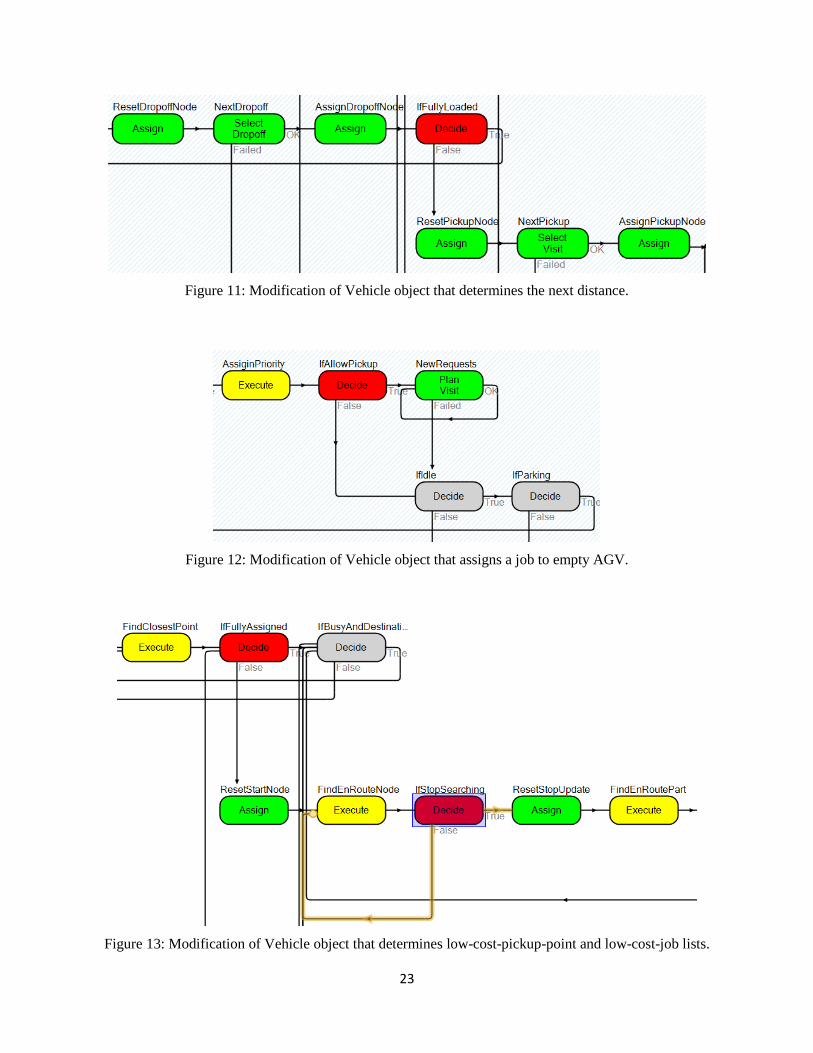
Figure 11: Modification of Vehicle object that determines the next distance. ........................................... 23
Figure 12: Modification of Vehicle object that assigns a job to empty AGV. ............................................ 23
Figure 13: Modification of Vehicle object that determines low-cost-pickup-point and low-cost-job lists. 23
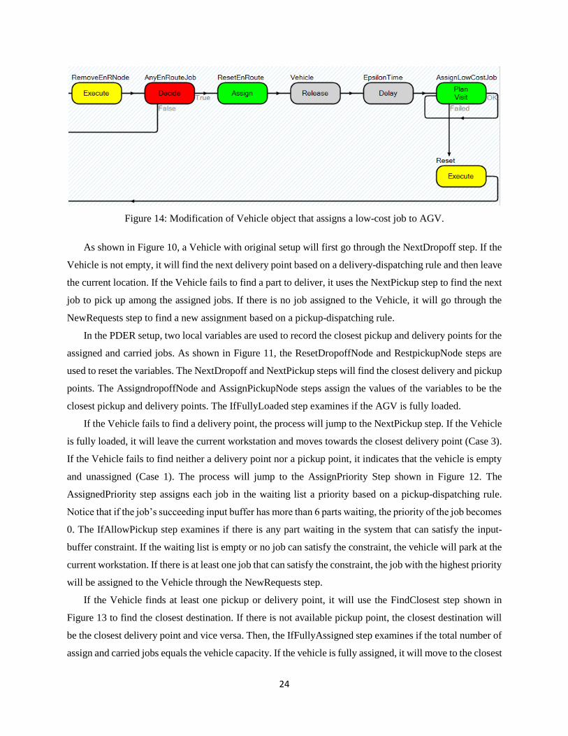
Figure 14: Modification of Vehicle object that assigns a low-cost job to AGV. ........................................ 24
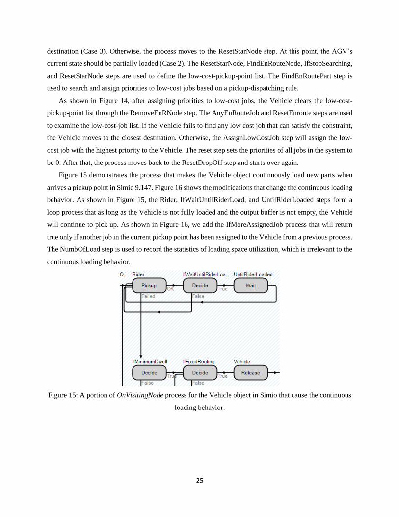
Figure 15: A portion of OnVisitingNode process for the Vehicle object in Simio. .................................... 25
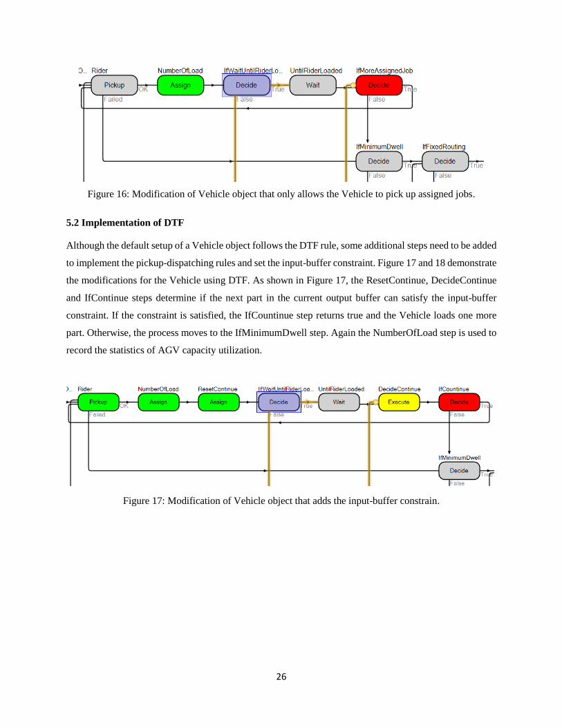
Figure 16: Modification of Vehicle object that only allows the Vehicle to pick up assigned jobs. ............ 26
Figure 17: Modification of Vehicle object that adds the input-buffer constrain. ........................................ 26
Figure 18: Modification of Vehicle object implement the pickup-dispatching rule using the DTF rule. ... 27
Figure 19: The WLB rule in Simio. ............................................................................................................ 28
Figure 20: Layout of FMS 1. ...................................................................................................................... 30
Figure 21: Layout of FMS 2 (Ho and Chien, 2006). ................................................................................... 31
Figure 22: System throughput results for experiment 1. ............................................................................. 32
Figure 23: Layout of FMS 3. ...................................................................................................................... 38
Figure 24: Throughput analysis of FMS 1 with dual-load AGVs in experiment 2. .................................... 39
Figure 25: Throughput analysis of FMS 1 with triple-load AGVs in experiment 2. .................................. 39
Figure 26: Throughput Analysis of FMS 1, experiment 2. ......................................................................... 41
Figure 27: AGV capacity utilization analysis in FMS 1, experiment 2. ..................................................... 41
Figure 28: Average travel distance of AGVs in FMS 1, experiment 2. ...................................................... 42
Figure 29: Throughput Analysis of FMS 3, experiment 2. ......................................................................... 44
Figure 30: AGV capacity utilization in FMS 2, experiment 2. ................................................................... 45
Figure 31: Average travel distance of AGVs in FMS 2, experiment 2. ...................................................... 46
Figure 32: Throughput Analysis of FMS 3, experiment 2. ......................................................................... 48
vii
Figure 33: AGV capacity utilization in FMS 3, experiment 2. ................................................................... 49
Figure 34: Average travel distance of AGVs in FMS 3, experiment 2. ...................................................... 49
Figure 35: Add-on process for the Source in Simio.. .................................................................................. 57
Figure 36: Theprocess invoked by the FindClosestPoint in Figure 13.. ..................................................... 57
Figure 37: The process invoked by FindEnRouteNode in Figure 13. ......................................................... 58
Figure 38: Th=e process invoked by FindEnRoutePart in Figure 13. ......................................................... 58
Figure 39: The process invoked by RemoveEnrouteNode in Figure 14. .................................................... 58
Figure 40: The process invoked by Reset in Figure 14 and 18. .................................................................. 59
Figure 41: The process invoked by DecideContinue in Figure 17. ............................................................. 59
Figure 42: The process invoked by the AssignPriority in Figure 12 and 18. .............................................. 59
Figure 43: Throughput Analysis of FMS 2 with dual-load AGVs. ............................................................. 60
Figure 44: Throughput Analysis of FMS 2 with triple-load AGVs. ........................................................... 60
Figure 45: Throughput Analysis of FMS 3 with dual-load AGVs. ............................................................. 61
Figure 46: Throughput Analysis of FMS 3 with triple-load AGVs. ........................................................... 61
Figure 47: AGV capacity utilization when using 2 (a) and 3 (b) dual-load AGVs in FMS 1. .................... 62
Figure 48: AGV capacity utilization when using 2 (a) and 3 (b) triple-load AGVs in FMS 1. .................. 62
Figure 49: AGV capacity utilization when using 2 (a) and 3 (b) dual-load AGVs in FMS 2. .................... 63
Figure 50: AGV capacity utilization when using 2 (a) and 3 (b) triple-load AGVs in FMS 2. .................. 63
Figure 51: AGV capacity utilization when using 2 (a) and 3 (b) dual-load AGVs in FMS 3. .................... 64
Figure 52: AGV capacity utilization when using 2 (a) and 3 (b) triple-load AGVs in FMS 3. .................. 64
viii
Notation
𝐵𝑎 A Boolean variable that indicates if workstation 𝑎 is blocked.
𝐶𝐼𝐵𝑏 Capacity of input buffer of workstation 𝑏.
𝐶𝑂𝑄𝑎 Capacity of output buffer of workstation 𝑎.
𝐷 The shortest distance between AGV, 𝑉, and job 𝑖.
𝐷𝑉 List of destinations for AGV, 𝑉, corresponding to its assigned and carried jobs.
𝑖 A transportation job (load) in the system.
𝐼 Waiting list of all unassigned jobs in the system.
𝐼𝑉 Set of low-cost jobs waiting at pickup points 𝑃𝑉 where 𝐼𝑉 ⊆ 𝐼.
𝐼𝐵𝑏 Input buffer of workstation 𝑏.
𝑁𝐼𝐵𝑏 number of parts in the input buffer of workstation 𝑏
𝑁𝑂𝐵𝑎 number of parts in the output buffer of workstation 𝑎
𝑂𝐵𝑎 Output buffer of workstation 𝑎.
𝑃𝑖 Priority of job 𝑖.
𝑃𝑉 List of pickup points located between the AGV’s current location and next destination.
𝑆𝑏 A Boolean variable that indicates if workstation 𝑏 is starved.
𝑉 An AGV in the system.
𝑊𝑆 A workstation in the system.
1
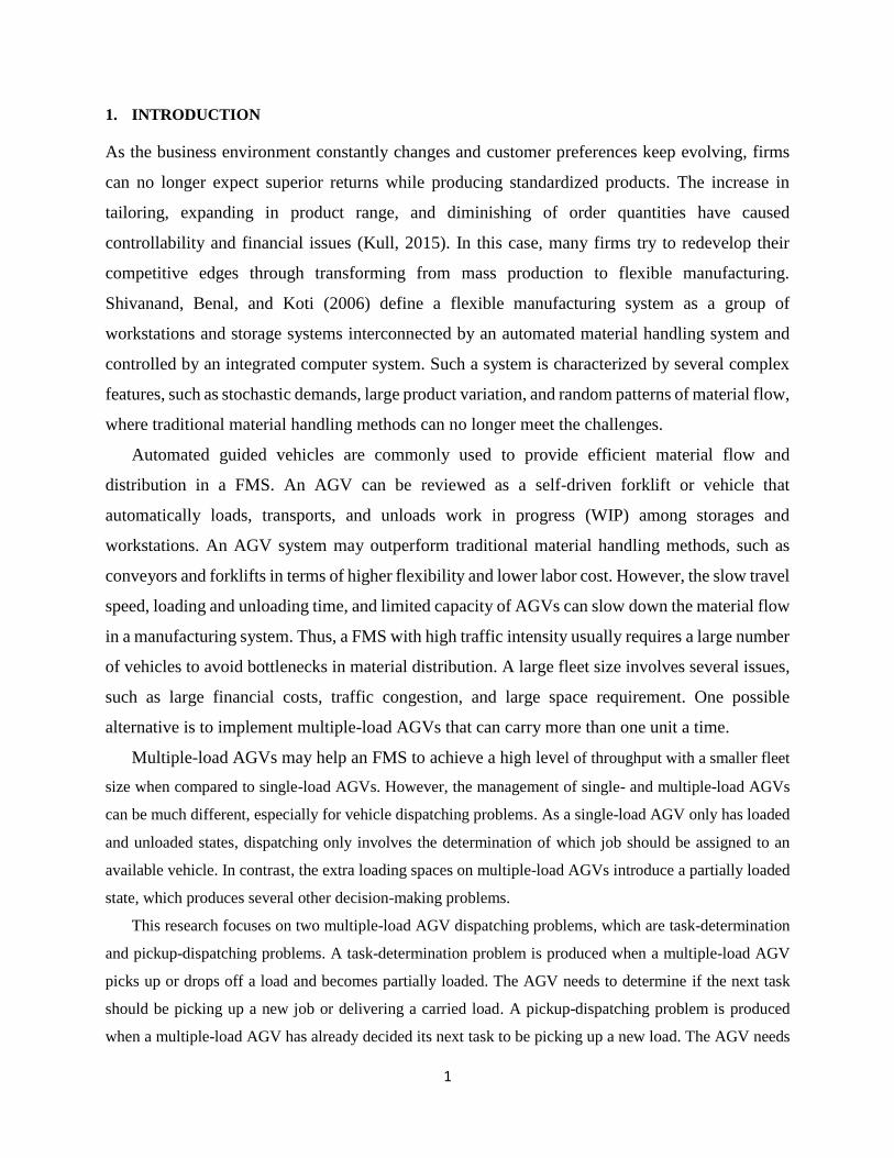
1. INTRODUCTION
As the business environment constantly changes and customer preferences keep evolving, firms
can no longer expect superior returns while producing standardized products. The increase in
tailoring, expanding in product range, and diminishing of order quantities have caused
controllability and financial issues (Kull, 2015). In this case, many firms try to redevelop their
competitive edges through transforming from mass production to flexible manufacturing.
Shivanand, Benal, and Koti (2006) define a flexible manufacturing system as a group of
workstations and storage systems interconnected by an automated material handling system and
controlled by an integrated computer system. Such a system is characterized by several complex
features, such as stochastic demands, large product variation, and random patterns of material flow,
where traditional material handling methods can no longer meet the challenges.
Automated guided vehicles are commonly used to provide efficient material flow and
distribution in a FMS. An AGV can be reviewed as a self-driven forklift or vehicle that
automatically loads, transports, and unloads work in progress (WIP) among storages and
workstations. An AGV system may outperform traditional material handling methods, such as
conveyors and forklifts in terms of higher flexibility and lower labor cost. However, the slow travel
speed, loading and unloading time, and limited capacity of AGVs can slow down the material flow
in a manufacturing system. Thus, a FMS with high traffic intensity usually requires a large number
of vehicles to avoid bottlenecks in material distribution. A large fleet size involves several issues,
such as large financial costs, traffic congestion, and large space requirement. One possible
alternative is to implement multiple-load AGVs that can carry more than one unit a time.
Multiple-load AGVs may help an FMS to achieve a high level of throughput with a smaller fleet
size when compared to single-load AGVs. However, the management of single- and multiple-load AGVs
can be much different, especially for vehicle dispatching problems. As a single-load AGV only has loaded
and unloaded states, dispatching only involves the determination of which job should be assigned to an
available vehicle. In contrast, the extra loading spaces on multiple-load AGVs introduce a partially loaded
state, which produces several other decision-making problems.
This research focuses on two multiple-load AGV dispatching problems, which are task-determination
and pickup-dispatching problems. A task-determination problem is produced when a multiple-load AGV
picks up or drops off a load and becomes partially loaded. The AGV needs to determine if the next task
should be picking up a new job or delivering a carried load. A pickup-dispatching problem is produced
when a multiple-load AGV has already decided its next task to be picking up a new load. The AGV needs

2
to determine which point the AGV should visit next. As multiple-load AGVs are managed by more efficient
task-determination and pickup-dispatching rules, we believe the system throughput and average time in
system of parts will be maximized and minimized respectively in a FMS.
3
2. PROBLEM STATEMENT
One common problem for AGV systems in FMSs is that they require a large number of AGVs to deal with
the dynamic environment and large product variation. Instead of moving material continuously like a
conveyor, an AGV transports material in a discrete manner, which increases the flexibility but reduces the
speed of material handling process. This is the reason that most AGV systems are only implemented in low
to medium production volume systems. One common way to improve the speed of material flow is to
increase the number of AGVs in the system. However, a large fleet size can produce several problems, such
as traffic congestion, large financial cost, and large requirement of space. One possible alternative is to
implement multiple-load AGVs that can carry most than one unit a time.
Despite the considerable amount of recent research on AGV dispatching rules, only few authors study
multiple-load AGVs in FMS. However, the management of single- and multiple-load AGVs are much
different. A single-load AGV only has empty and loaded states. When the AGV is empty, it only needs to
decide which load should be picked up next. When the AGV is loaded, it only needs to find the destination
of the carried load. The additional loading spaces on multiple-load AGVs introduce a partially loaded state.
When an AGV is partially loaded, it needs to determine if the next task should be picking up a new load or
dropping off a carried load, which is a task-determination problem. It is found that many researchers
studying multiple-load AGVs use a delivery-task-first (DTF) rule to deal with the task determination
problem. The DTF rule suggests that an AGV should always choose to deliver parts when it is partially
loaded. However, as the DTF rule gives delivery tasks higher priorities, after an AGV drops off a load, the
empty loading space will not be utilized until the AGV frees up all loading spaces. Such a problem will
reduce the AGV capacity utilization and hence limits the system throughput.
It is found that most of pickup-dispatching rules are designed for single-load AGVs. Some researchers
apply single-attribute rules on multiple-load AGVs to test their performances. As many researchers found
that multi-attribute dispatching rules usually outperform single-attribute dispatching rules in terms of
system throughput and average time in system, we believe the benefits of multiple-load AGVs are not fully
captured by applying single-attribute dispatching rules.
There are two parallel objectives in this research. First we want to develop a task-determination rule
and a pickup-dispatching rule that can increase the AGV capacity utilization and machine utilization
respectively and hence improve the system throughput. The second objective is to use simulation
experiments to examine both rules and compare them with the existing task-determination and pickup-
dispatching rules.
4
3. LITERATURE REVIEW
This section reviews the previous research on automated guided vehicle management. The common ways
to manage the coordination of AGVs are introduced and compared. The previous researches on multiple-
load AGVs are demonstrated. The classification of AGV dispatching algorithm is summarized, and some
common dispatching rules are introduced. Finally, the major findings from the literature review are
discussed.
3.1 Scheduling vs. Dispatching
According to Vivaldini, Rocha, Becker, and Moreira (2015), the major design challenge of an AGV system
is to assure that vehicles efficiently arrive to the desired destinations at the desired time within highly
dynamic environments so that traffic conflicts, machine overloads, starvations, and other unpredicted events
will be avoided. The most common approaches to manage the coordination among AGVs are dispatching
and scheduling. Original AGV dispatching was defined as a function that assigns transportation tasks to
vehicles, where scheduling determines the time at which vehicles should enter and leave the guide-path
segments to avoid conflicts (Langevin, Lauzon, & Riopel, 1996). However, in recent years, scheduling
becomes a task allocation process for AGVs considering the time and cost of operations (Corréa, Langevin,
& Rousseau, 2007). A scheduling system can decide when, where, and how a vehicle performs tasks
including the route it should take (Le-Anh & De Koster, 2006). With an on-line scheduling system, these
decisions are specified and updated after a time horizon (Yang, Jaillet, & Mahmassani, 2004).
An AGV system designer can think of dispatching as a scheduling system with zero time horizon so
that decisions are made once a vehicle reaches its destination or a new request is generated. Le-Anh et al.
(2006) have conducted a comprehensive review study that lists pros and cons of dispatching and scheduling.
Dispatching algorithms are typically more favorable in a highly stochastic environment, since it is difficult
to schedule vehicles over a long period in such an uncertain environment. In case of a high job density,
AGVs frequently move from one workstation to another so that a complicated scheduling system may not
be as useful. Four common objectives of AGV dispatching rules are minimizing average time in system of
parts, maximizing system throughput, minimizing queue length, and guaranteeing a certain service level at
stations (Le-Anh and De Koster, 2006).
3.2 Multiple-load AGV Dispatching
Despite the considerable amount of research on AGV dispatching, only a few authors study multiple-load
AGVs. Johnson and Brandeau (1995) conduct a study to compare the performances of single-load and
multiple-load AGVSs in a central depot. The results show that multiple-load AGVs are capable of serving
more stations without increasing the mean response time. Grunow, Günther, and Lehmann (2004) present
5
a simulation on multiple-load AGVs in a highly automated seaport container terminal. The numerical results
indicate that using dual-load AGVs can significantly improve the system efficiency with respect to average
lateness and berthing time when compare to single-load AGVs. Ozden (1988) conducts a study to compare
the performance of single- and multiple-load AGVs in an FMS. The results show that multiple-load AGVs
can often help an FMS to achieve a higher level of throughput with a smaller fleet size. Some other benefits
of multiple-load AGVs include improving machine utilizations and better utilization of AGVs (Bilge and
Tanchoco, 1997).
The major challenge of managing multiple-load AGVs is that the additional loading spaces increases
the number of decision-making states. According to Ho and Chien (2006), a single-load AGV only has two
decision-making states, which are empty and loaded, while a multiple-load AGV can be empty, partially
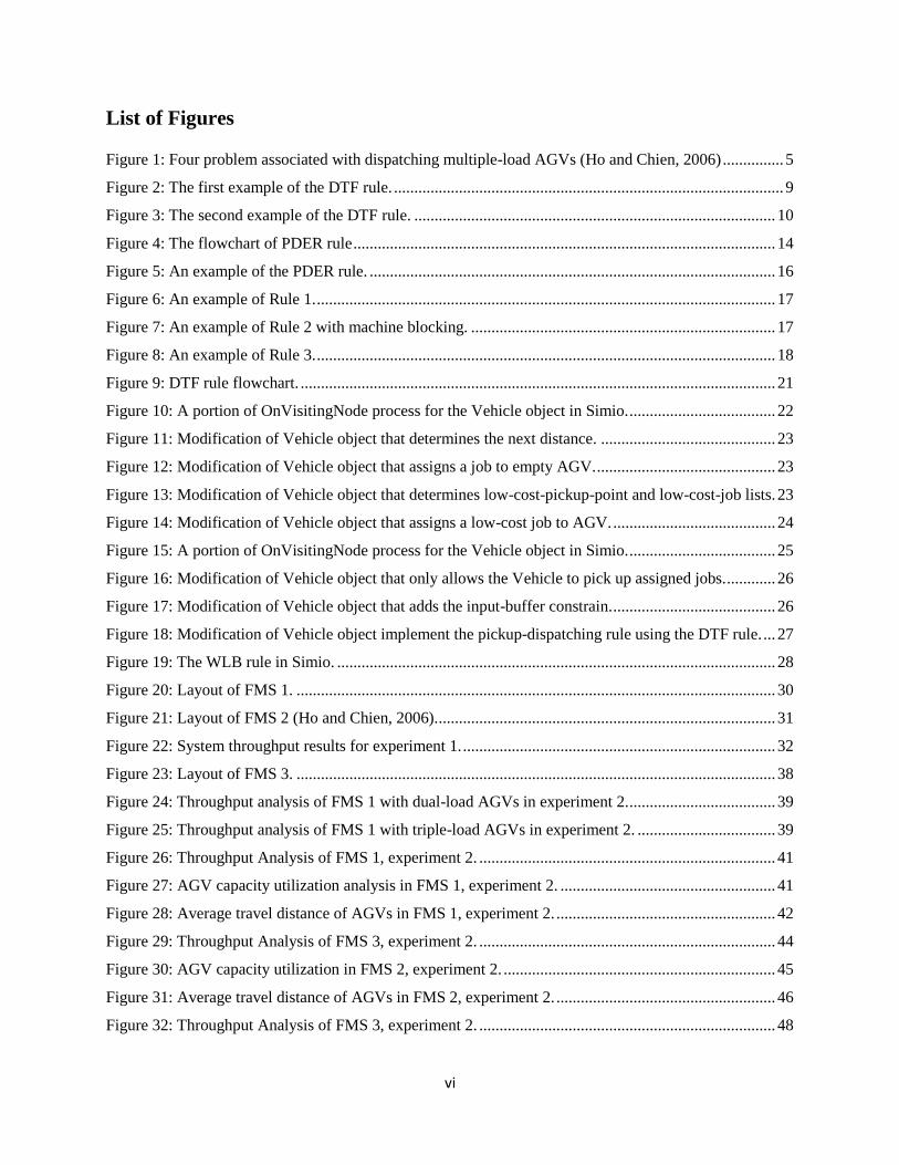
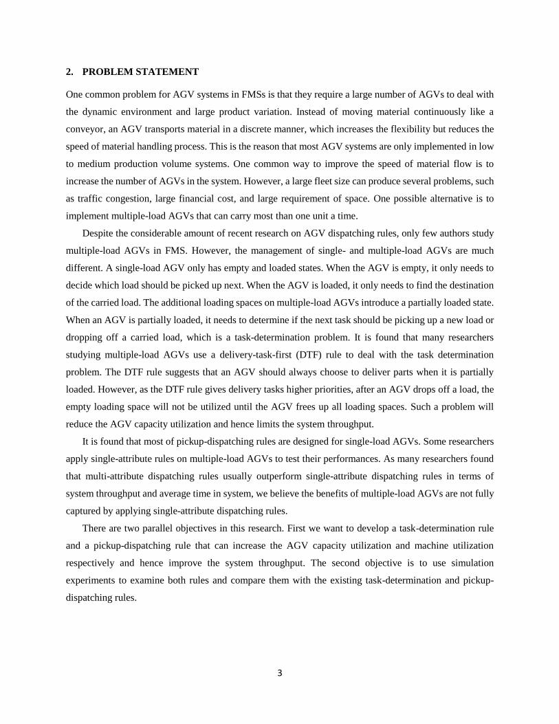
loaded, and fully loaded. As shown in Figure 1, Ho and Chien (2006) define four major problems associated
with dispatching multiple-load AGVs, which are,
Task-determination problem: determines if the AGV’s next task should be picking up a new job or
dropping off a carried load when it is partially loaded.
Pickup-dispatching problem: determines which pickup point should the AGV visits when the
vehicle has already decided its next task to be picking up a new load.
Delivery-dispatching problem: determines which load should be delivered next when the AGV has
already decided its next task to be delivering a carried load.
Task-selection problem: determines which load should be picked up when the AGV is visiting a
pickup point.
Figure 1: Four problem associated with dispatching multiple-load AGVs (Ho and Chien, 2006)
6
Ho and Chien (2006) propose three rules to handle the task-determination problem. The pickup-task-
first (PTF) rule indicates that when an AGV is partially loaded, it should always pick up new loads until it
becomes full. A delivery-task-first (DTF) rule suggests that an AGV should always perform a delivery task
when it is partially loaded. With either the PTF or DTF rule, an AGV should pick up as many parts as it
can at a pickup point. Rather than giving the pickup or delivery task a higher priority, a load-ratio (LR) rule
determines the AGV’s next task based on the load ratio on the vehicle. In order to compare the performance
of these task-determination rules, Ho and Chien (2006) couple them with different delivery-dispatching
rules and test them in a representitive FMS through simulation models. The results show that the DTF rule
is more favorable in terms of maximizing throughput and minimizing average time in system. Based on
their results, other authors also examine different pickup-dispatching, delivery-dispatching, and load-
selection rules (Ho and Liu 2006, Ho and Liu 2009).
Azimi, Haleh, and Alidoost (2010) study pickup-dispatching and delivery-dispatching rules for
multiple-load AGVs in an FMS. To evaluate the performances of different combinations of rules, the
authors develop a fuzzy multi-attribute decision-making method that takes into account ten performance
criteria, including system throughput (ST), mean flow time of parts (MFTP), mean tardiness of parts
(MFTP), AGV idle time (AGVIT), AGV travel full (AGVTF), AGV travel empty (AGVTE), AGV load
time (AGVLT), AGV unload time (AGVUT), mean queue length (MQL), and mean queue waiting (MQW).
Their findings indicate that the best pickup-dispatching rule is Earliest Due Time (EDT), and the best
delivery-dispatching rule is Shortest Distance (SD).
3.3 Workcenter-initiated vs. Vehicle-initiated Dispatching Rules
Pickup-dispatching rules can be categorized as either workcenter-initiated or vehicle-initiated rules
(Egbelu, & Tanchoco, 1984). A workcenter-initiated rule involves the selection of a vehicle from a set of
idle vehicles to be assigned to a transportation job. A vehicle-initiated rule involves the selection of a job
from a set of unassigned jobs when there is only one available vehicle. Some well-known dispatching rules,
first recognized in 1980s, are listed below. Notice that these rules are the key components of multi-attribute
algorithms that are popular today.
A. Workcenter-initiated rules (single request and multiple vehicles):
a) Random Vehicle Rule (RV): the request is randomly assigned to any available vehicle.
b) Nearest Vehicle Rule (NV): the vehicle with the shortest travel distance to the pickup point is
dispatched.
c) Farthest Vehicle Rule (FV): an antithetical rule that dispatches the vehicle who has the longest
travel distance to the pickup point.
7
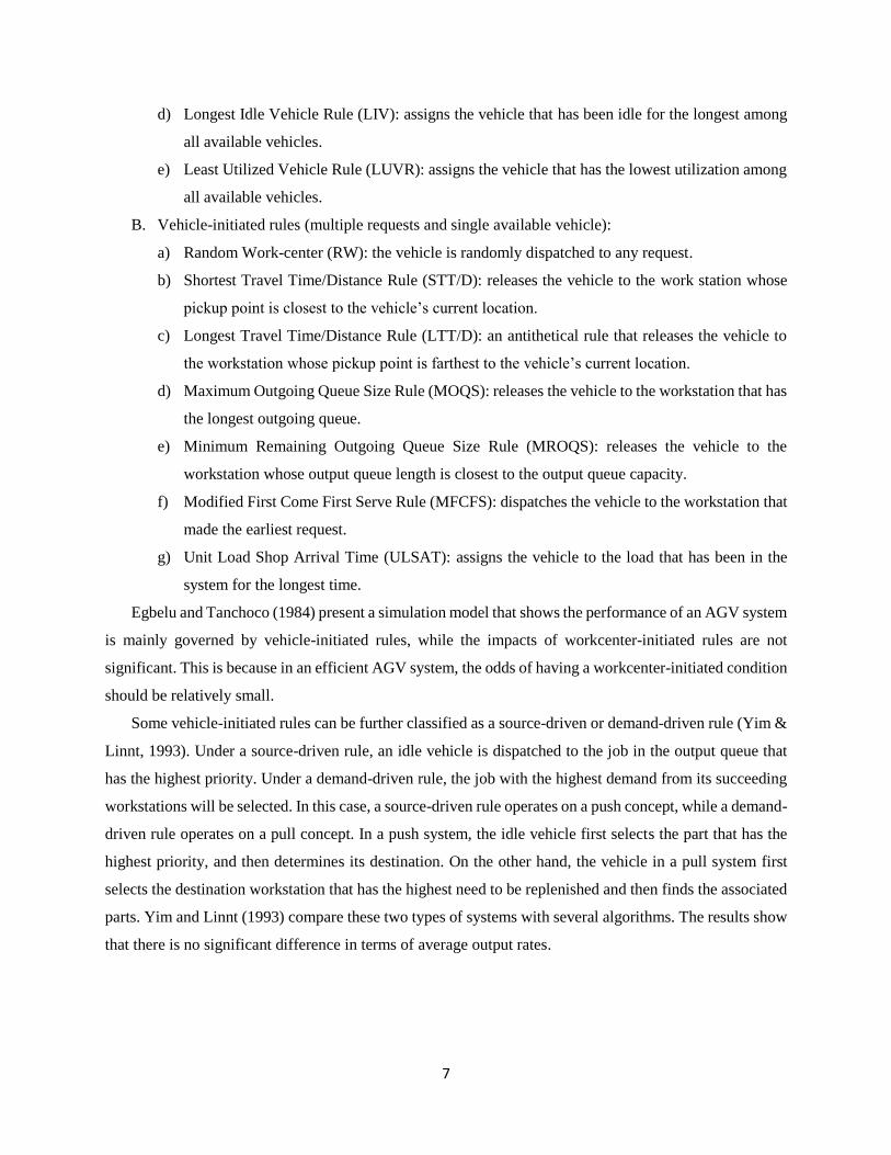
d) Longest Idle Vehicle Rule (LIV): assigns the vehicle that has been idle for the longest among
all available vehicles.
e) Least Utilized Vehicle Rule (LUVR): assigns the vehicle that has the lowest utilization among
all available vehicles.
B. Vehicle-initiated rules (multiple requests and single available vehicle):
a) Random Work-center (RW): the vehicle is randomly dispatched to any request.
b) Shortest Travel Time/Distance Rule (STT/D): releases the vehicle to the work station whose
pickup point is closest to the vehicle’s current location.
c) Longest Travel Time/Distance Rule (LTT/D): an antithetical rule that releases the vehicle to
the workstation whose pickup point is farthest to the vehicle’s current location.
d) Maximum Outgoing Queue Size Rule (MOQS): releases the vehicle to the workstation that has
the longest outgoing queue.
e) Minimum Remaining Outgoing Queue Size Rule (MROQS): releases the vehicle to the
workstation whose output queue length is closest to the output queue capacity.
f) Modified First Come First Serve Rule (MFCFS): dispatches the vehicle to the workstation that
made the earliest request.
g) Unit Load Shop Arrival Time (ULSAT): assigns the vehicle to the load that has been in the
system for the longest time.
Egbelu and Tanchoco (1984) present a simulation model that shows the performance of an AGV system
is mainly governed by vehicle-initiated rules, while the impacts of workcenter-initiated rules are not
significant. This is because in an efficient AGV system, the odds of having a workcenter-initiated condition
should be relatively small.
Some vehicle-initiated rules can be further classified as a source-driven or demand-driven rule (Yim &
Linnt, 1993). Under a source-driven rule, an idle vehicle is dispatched to the job in the output queue that
has the highest priority. Under a demand-driven rule, the job with the highest demand from its succeeding
workstations will be selected. In this case, a source-driven rule operates on a push concept, while a demand-
driven rule operates on a pull concept. In a push system, the idle vehicle first selects the part that has the
highest priority, and then determines its destination. On the other hand, the vehicle in a pull system first
selects the destination workstation that has the highest need to be replenished and then finds the associated
parts. Yim and Linnt (1993) compare these two types of systems with several algorithms. The results show
that there is no significant difference in terms of average output rates.
8
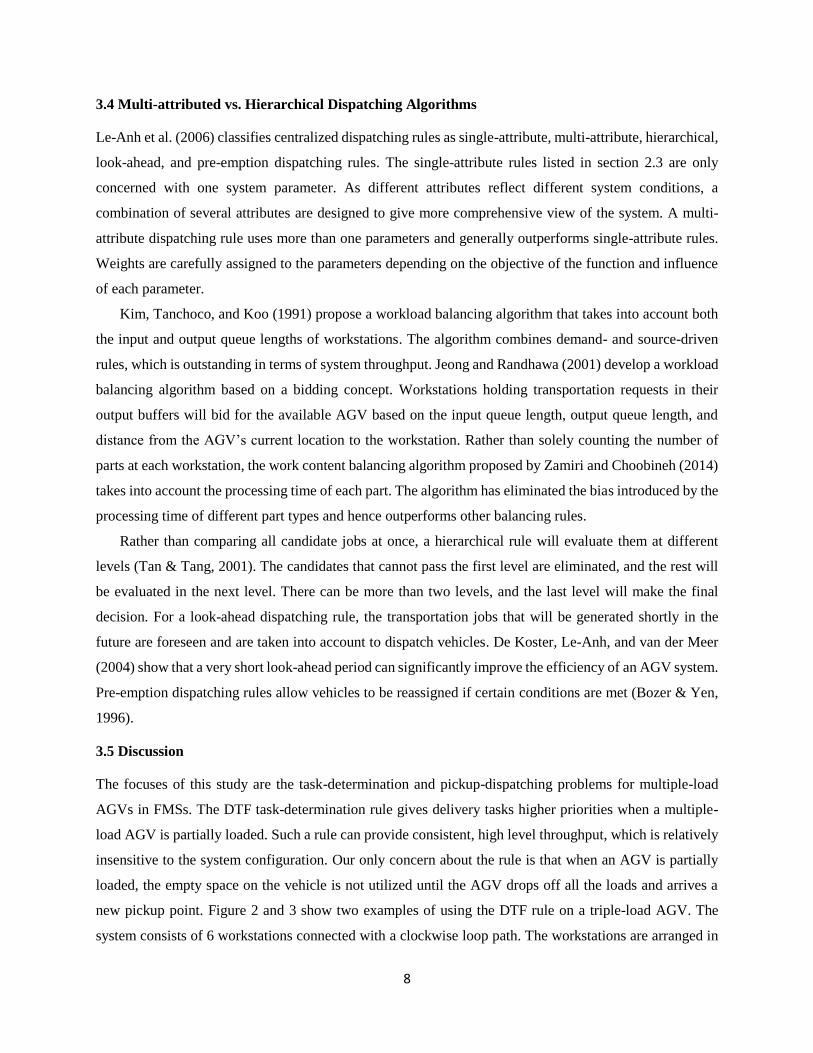
3.4 Multi-attributed vs. Hierarchical Dispatching Algorithms
Le-Anh et al. (2006) classifies centralized dispatching rules as single-attribute, multi-attribute, hierarchical,
look-ahead, and pre-emption dispatching rules. The single-attribute rules listed in section 2.3 are only
concerned with one system parameter. As different attributes reflect different system conditions, a
combination of several attributes are designed to give more comprehensive view of the system. A multi-
attribute dispatching rule uses more than one parameters and generally outperforms single-attribute rules.
Weights are carefully assigned to the parameters depending on the objective of the function and influence
of each parameter.
Kim, Tanchoco, and Koo (1991) propose a workload balancing algorithm that takes into account both
the input and output queue lengths of workstations. The algorithm combines demand- and source-driven
rules, which is outstanding in terms of system throughput. Jeong and Randhawa (2001) develop a workload
balancing algorithm based on a bidding concept. Workstations holding transportation requests in their
output buffers will bid for the available AGV based on the input queue length, output queue length, and
distance from the AGV’s current location to the workstation. Rather than solely counting the number of
parts at each workstation, the work content balancing algorithm proposed by Zamiri and Choobineh (2014)
takes into account the processing time of each part. The algorithm has eliminated the bias introduced by the
processing time of different part types and hence outperforms other balancing rules.
Rather than comparing all candidate jobs at once, a hierarchical rule will evaluate them at different
levels (Tan & Tang, 2001). The candidates that cannot pass the first level are eliminated, and the rest will
be evaluated in the next level. There can be more than two levels, and the last level will make the final
decision. For a look-ahead dispatching rule, the transportation jobs that will be generated shortly in the
future are foreseen and are taken into account to dispatch vehicles. De Koster, Le-Anh, and van der Meer
(2004) show that a very short look-ahead period can significantly improve the efficiency of an AGV system.
Pre-emption dispatching rules allow vehicles to be reassigned if certain conditions are met (Bozer & Yen,
1996).
3.5 Discussion
The focuses of this study are the task-determination and pickup-dispatching problems for multiple-load
AGVs in FMSs. The DTF task-determination rule gives delivery tasks higher priorities when a multiple-
load AGV is partially loaded. Such a rule can provide consistent, high level throughput, which is relatively
insensitive to the system configuration. Our only concern about the rule is that when an AGV is partially
loaded, the empty space on the vehicle is not utilized until the AGV drops off all the loads and arrives a
new pickup point. Figure 2 and 3 show two examples of using the DTF rule on a triple-load AGV. The
system consists of 6 workstations connected with a clockwise loop path. The workstations are arranged in
9
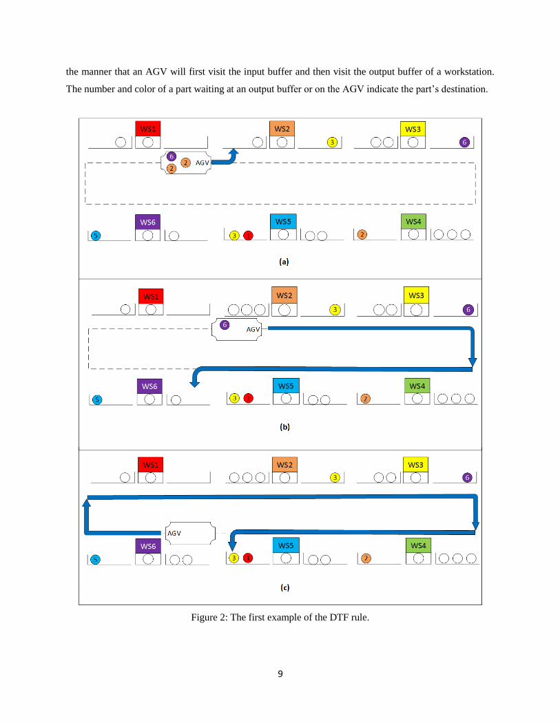
the manner that an AGV will first visit the input buffer and then visit the output buffer of a workstation.
The number and color of a part waiting at an output buffer or on the AGV indicate the part’s destination.
Figure 2: The first example of the DTF rule.
10
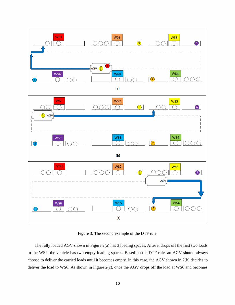
Figure 3: The second example of the DTF rule.
The fully loaded AGV shown in Figure 2(a) has 3 loading spaces. After it drops off the first two loads
to the WS2, the vehicle has two empty loading spaces. Based on the DTF rule, an AGV should always
choose to deliver the carried loads until it becomes empty. In this case, the AGV shown in 2(b) decides to
deliver the load to WS6. As shown in Figure 2(c), once the AGV drops off the load at WS6 and becomes
11
empty, it chooses the next pickup point to be the output buffer of WS5. In this example, the two empty
loading spaces have not been utilized since the first two loads are dropped at the beginning.
Another problem is that when the AGV decides to visit a pickup point, the output queue of the
workstation may not have enough loads to fill up the vehicle. In such a case, the empty space will not be
utilized until the AGV delivers all parts loaded from this output queue. As shown in Figure 3(a), the triple-
load AGV only finds two parts from the output buffer of the WS5. The AGV picks the loads and deliver
them to the WS1 and WS3 respectively. After it drops off the last load, it chooses the input buffer of the
WS4 as its next pickup point. In this example, the AGV has an empty loading space since the beginning.
The objective of this study is to develop a combination of task-determination and pickup-dispatching
rules that can increase the system throughput and decrease the average time in system. The first step of this
study is to develop a task-determination rule that improves the utilizations of loading spaces for multiple-
load AGVs. The two problems shown in examples should be avoided, which may speed up the material
flow in a FMS. The second step is to develop a workload-balancing dispatching algorithm tailored for
multiple-load AGVs. The previous studies show that multi-attribute, pickup-dispatching algorithm usually
outperforms single-attribute rules on single-load AGVs, especially when employing a workload balancing
concept. As the workload balancing rule can avoid machine blocking and starvation, the machine utilization
should be improved. We believe the faster material flow and higher machine utilization may lead to a higher
system throughput and smaller average time in system.
12
4. ALGORITHM DESIGN
In this section, we first introduce the pickup-or-delivery-en-route rule that deals with the task-determination
problem. Then, we explain the workload balancing rule that is used for the pickup-dispatching problem.
Besides the task-termination and pickup-dispatching rules, some other AGV control rules employed on the
AGVs in the experiment are described. Finally, we introduce the task-determination rules and the pickup-
dispatching rules that are used to compare with the PDER and WLB rules, respectively.
4.1 Pickup-or-Delivery-En-Route Rule
The task-determination rule proposed in this study is the pickup-or-delivery-en-route rule. The essential
goal of the PDER rule is to maximize the utilization of loading spaces on multiple-load AGVs. The
utilization can be increased by allowing a partially loaded AGV to pick up additional loads on its way
moving towards the next destination. The PDER rule suggests that when a multiple-load AGV just
completes all the necessary tasks at a pickup or delivery point and becomes partially loaded, it should search
for a new assignment among the jobs whose pickup points are geographically located on the shortest path
between the AGV’s current location and next destination. These jobs are named as low-cost jobs because
it is very convenient for the AGV to pick them up. The next destination is the closest pickup or delivery
point corresponding to a job that have been assigned to or carried by the AGV.
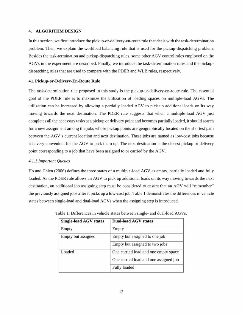
4.1.1 Important Queues
Ho and Chien (2006) defines the three states of a multiple-load AGV as empty, partially loaded and fully
loaded. As the PDER rule allows an AGV to pick up additional loads on its way moving towards the next
destination, an additional job assigning step must be considered to ensure that an AGV will “remember”
the previously assigned jobs after it picks up a low-cost job. Table 1 demonstrates the differences in vehicle
states between single-load and dual-load AGVs when the assigning step is introduced.
Table 1: Differences in vehicle states between single- and dual-load AGVs.
Single-load AGV states Dual-load AGV states
Empty Empty
Empty but assigned Empty but assigned to one job
Empty but assigned to two jobs
Loaded One carried load and one empty space
One carried load and one assigned job
Fully loaded
13
With a PDER rule, a transportation job 𝑖 will be kept in any one of the three queues: the waiting list, 𝐼,
presents all unassigned jobs in the system; an AGV’s assignment list indicates the jobs that have been
assigned to the AGV; and an AGV’s workload list demonstrates the jobs that have been picked up and
carried by the AGV. Once a job is assigned to an AGV, it will be removed from the waiting list of the
system and added to the AGV’s assignment list. As the job is picked up by the AGV, it will be transferred
from the AGV’s assignment list to the workload list. Finally, the job will be removed from the workload
list when the AGV drops it off at its destination.
A destination list, 𝐷𝑉 , is a list of destinations for AGV, 𝑉, corresponding to its assigned and carried
jobs. For each time 𝑉 is assigned to a new job, the pickup point (𝑂𝐵𝑎) and drop-off point (𝐼𝐵𝑏) of the job
will be added to 𝐷𝑉. As 𝑉 picks up or drops off a job, 𝐵𝑂𝑎 or 𝐼𝐵𝑏 will be removed from 𝐷𝑉 respectively.
An AGV’s low-cost-pickup-point list 𝑃𝑉 is a list of pickup points that geometrically locate between the
AGV’s current location and next destination (including the current location and next destination). An
AGV’s low-cost-job list 𝐼𝑉 ⊆ 𝐼 is a subset of the waiting list that records all jobs waiting at the low-cost-
pickup points. These jobs are considered to have low costs since it is very convenient for the AGV to pick
them up.
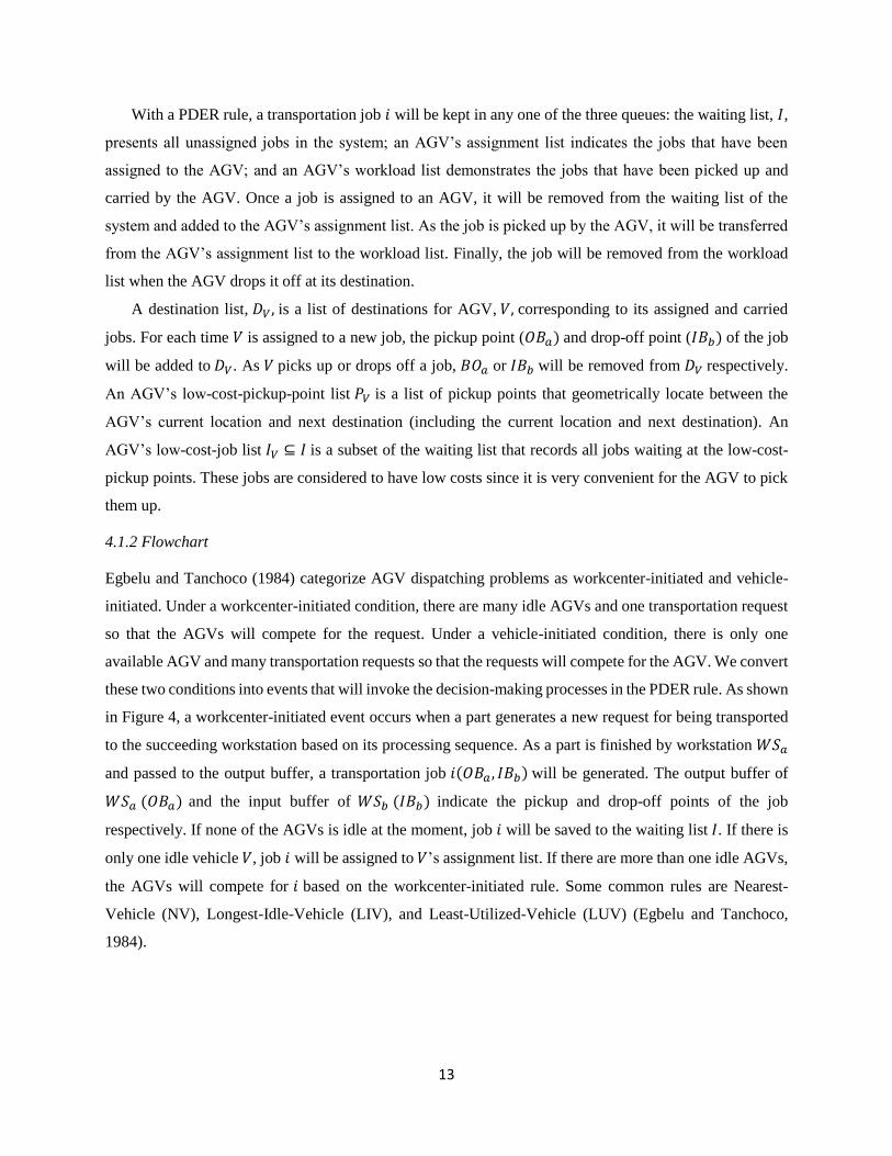
4.1.2 Flowchart
Egbelu and Tanchoco (1984) categorize AGV dispatching problems as workcenter-initiated and vehicle-
initiated. Under a workcenter-initiated condition, there are many idle AGVs and one transportation request
so that the AGVs will compete for the request. Under a vehicle-initiated condition, there is only one
available AGV and many transportation requests so that the requests will compete for the AGV. We convert
these two conditions into events that will invoke the decision-making processes in the PDER rule. As shown
in Figure 4, a workcenter-initiated event occurs when a part generates a new request for being transported
to the succeeding workstation based on its processing sequence. As a part is finished by workstation 𝑊𝑆𝑎
and passed to the output buffer, a transportation job 𝑖(𝑂𝐵𝑎 , 𝐼𝐵𝑏) will be generated. The output buffer of
𝑊𝑆𝑎 (𝑂𝐵𝑎) and the input buffer of 𝑊𝑆𝑏 (𝐼𝐵𝑏) indicate the pickup and drop-off points of the job
respectively. If none of the AGVs is idle at the moment, job 𝑖 will be saved to the waiting list 𝐼. If there is
only one idle vehicle 𝑉, job 𝑖 will be assigned to 𝑉’s assignment list. If there are more than one idle AGVs,
the AGVs will compete for 𝑖 based on the workcenter-initiated rule. Some common rules are Nearest-
Vehicle (NV), Longest-Idle-Vehicle (LIV), and Least-Utilized-Vehicle (LUV) (Egbelu and Tanchoco,
1984).
14
Figure 4: The flowchart of PDER rule
A vehicle-initiated event occurs when an AGV reaches a pickup or delivery point. As shown in Figure
4, when an AGV reaches a point, it will first perform the pickup or drop-off task that is pre-determined for
the assigned or carried job respectively. Notice that rather than picking up as many parts as the AGV can
like a DTF rule, the PDER rule only allows the AGV to pick up the jobs in it its assignment list. Once the
AGV completes the pre-determined task, it will be in one of the three conditions:
Case 1: 𝑉 is not carrying any load nor being assigned to any job. In this case, if the waiting list I is
not empty, 𝐴𝐺𝑉𝑛 will use a pickup-dispatching rule to determine the next pickup point and a load-
selection rule to decide the next pickup job. Otherwise, 𝑉 will park at the nearest parking area.
15
Case 2: As 𝑉 is assigned to or carrying one or more loads, it will first define its next destination,
which is the closest pickup or drop-off point in its destination list 𝐷𝑣. If the total number of jobs
assigned to and carried by 𝑉 is smaller than the vehicle capacity, 𝑉 will define its low-cost-pickup-
point list 𝑃𝑉 and low-cost-job list 𝐼𝑉. If 𝐼𝑉 is not empty, 𝑉 will use a pickup-dispatching rule to
determine the low-cost-pickup point that has the highest priority. A low-cost job waiting at this
pickup point will be selected based on the task-selection rule. If 𝐼𝑉 is empty, 𝑉 will move to the
next destination.
Case 3: As 𝑉 is assigned to or carrying one or more loads, it will first define its next destination.
The total number of assigned and carried jobs equals vehicle capacity. In this case, 𝑉 will move to
the next destination.
In Case 1 and 2, after i is assigned to 𝑉 and removed from 𝐼, 𝑉’s subsequent states will follow either
Case 2 or Case 3. In other words, 𝑉 will not leave the pickup or drop-off point unless the vehicle is fully
assigned, 𝐼 in Case 1 is empty, or 𝐼𝑉 in Case 2 is empty. As the next destination is defined as the closest
pickup or drop-off point in 𝑉’s destination list, the delivery-dispatching decisions always follow the STD
rule.
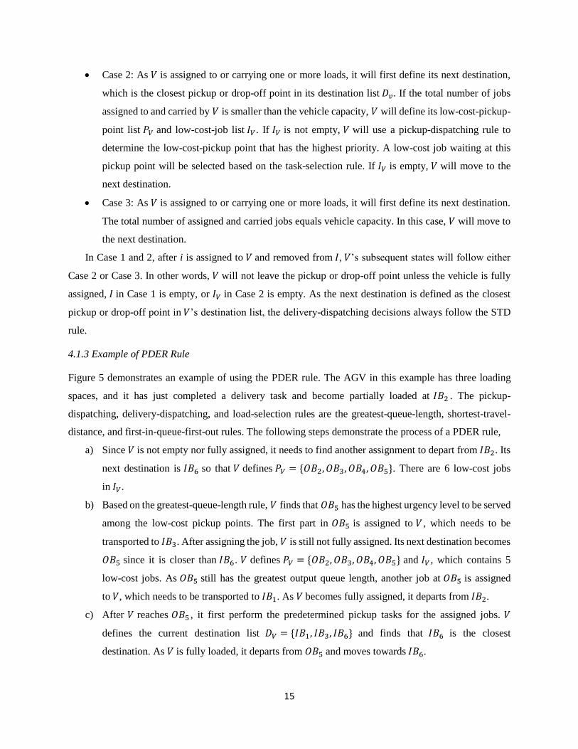
4.1.3 Example of PDER Rule
Figure 5 demonstrates an example of using the PDER rule. The AGV in this example has three loading
spaces, and it has just completed a delivery task and become partially loaded at 𝐼𝐵2 . The pickup-
dispatching, delivery-dispatching, and load-selection rules are the greatest-queue-length, shortest-travel-
distance, and first-in-queue-first-out rules. The following steps demonstrate the process of a PDER rule,
a) Since 𝑉 is not empty nor fully assigned, it needs to find another assignment to depart from 𝐼𝐵2. Its
next destination is 𝐼𝐵6 so that 𝑉 defines 𝑃𝑉 = {𝑂𝐵2, 𝑂𝐵3, 𝑂𝐵4, 𝑂𝐵5}. There are 6 low-cost jobs
in 𝐼𝑉.
b) Based on the greatest-queue-length rule, 𝑉 finds that 𝑂𝐵5 has the highest urgency level to be served
among the low-cost pickup points. The first part in 𝑂𝐵5 is assigned to 𝑉 , which needs to be
transported to 𝐼𝐵3. After assigning the job, 𝑉 is still not fully assigned. Its next destination becomes
𝑂𝐵5 since it is closer than 𝐼𝐵6. 𝑉 defines 𝑃𝑉 = {𝑂𝐵2, 𝑂𝐵3, 𝑂𝐵4, 𝑂𝐵5} and 𝐼𝑉 , which contains 5
low-cost jobs. As 𝑂𝐵5 still has the greatest output queue length, another job at 𝑂𝐵5 is assigned
to 𝑉, which needs to be transported to 𝐼𝐵1. As 𝑉 becomes fully assigned, it departs from 𝐼𝐵2.
c) After 𝑉 reaches 𝑂𝐵5 , it first perform the predetermined pickup tasks for the assigned jobs. 𝑉
defines the current destination list 𝐷𝑉 = {𝐼𝐵1, 𝐼𝐵3, 𝐼𝐵6} and finds that 𝐼𝐵6 is the closest
destination. As 𝑉 is fully loaded, it departs from 𝑂𝐵5 and moves towards 𝐼𝐵6.
16
Figure 5: An example of the PDER rule.
17
4.2 Workload Balancing Rule
4.2.1 Workload Balancing Concept
The proposed pickup-dispatching rule operates on a bidding concept. When an AGV becomes empty or
partially loaded, the jobs in 𝐼 or 𝐼𝑉 will bid for the AGV, respectively. The job with the highest bidding
score will win the auction. The bidding score is based on a workload-balancing concept. The essential goal
is to avoid machine blocking and starvation and hence improve the throughput.
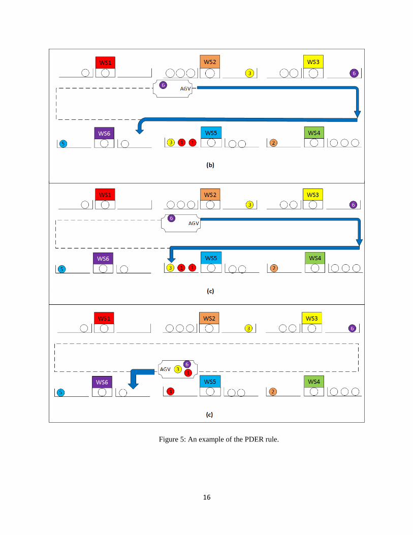
Four rules are used to rank job priorities. For Rule 1, if the delivery of a job can avoid both machine
blocking and starvation problems, such a job should have the highest priority. Figure 6 gives an example
of Rule 1. All parts waiting at 𝑂𝐵1 need to be transported to 𝐼𝐵2 and parts at 𝑂𝐵3 need to be delivered
to 𝐼𝐵4. We only consider the two parts at the beginning of the output queues at WS1 and WS3. All the
output and input buffer capacities are 3. As there is a machine blocking at WS1 and WS3 and a starvation
at WS2, the part at 𝑂𝐵1 has a higher priority.
For Rule 2, if the delivery of a job can avoid a machine blocking or starvation problem, such a job
should have a high priority. Figure 7 gives an example of Rule 2. A machine blocking occurs at WS1, and
there is no machine blocking at WS3 nor starvation at WS4. In this case, the part waiting at 𝑂𝐵1 has a
higher priority.
Figure 6: An example of Rule 1.
Figure 7: An example of Rule 2 with machine blocking.
18
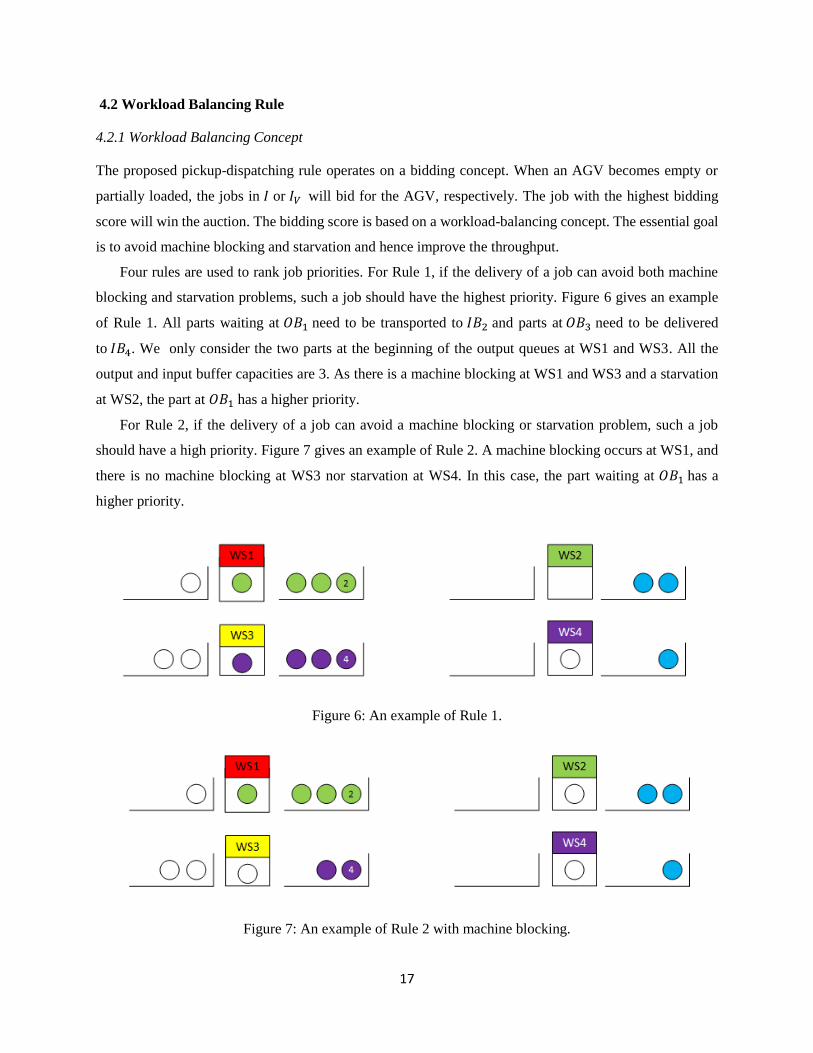
For Rule 3, a workstation that is closer to have a machine blocking or starvation should have a higher
priority. Figure 8 demonstrate an example of Rule 3. There is no machine blocking nor starvation observed
in the system. However, there are more parts waiting at 𝑂𝐵1 when compare to 𝑂𝐵2 so that WS1 is closer
to a machine blocking. In this case, the part waiting at 𝑂𝐵1 has a higher priority. For Rule 4, a shortest-
travel-distance rule is applied to break the tie. If multiple jobs tie by using Rule 1, 2, and 3, the job whose
pickup point is closer to the AGV’s current location will have a higher priority.
Figure 8: An example of Rule 3.
4.2.2 Job Evaluation
We convert the job ranking rules into a compound algorithm. When 𝑉 arrives a pickup or delivery point
(𝐼𝐵𝑐/𝑂𝐵𝑑 ). If 𝐼 in Case 1 or 𝐼𝑉 in Case 2 is not empty, 𝑉 will evaluate the score of each job in the list. The
score of job 𝑖(𝑂𝐵𝑎 , 𝐼𝐵𝑏) is determined by,
𝑃𝑖 = 𝐵𝑎 ∗ 100 + 𝑆𝑏 ∗ 100 + 10 ∗ (𝑁𝑂𝑄𝑎
𝐶𝑂𝑄𝑎+
𝐶𝐼𝑄𝑏 − 𝑁𝐼𝑄𝑏
𝐶𝐼𝑄𝑏) +
1
𝐷 + 1. (1)
The term 𝐵𝑎 is a Boolean variable that indicates if there is a machine blocking at 𝑖’s current output
buffer 𝑂𝐵𝑎, while 𝑆𝑏 specifies if there is a starvation at 𝑖’s succeeding buffer 𝐼𝐵𝑏. The term 𝑁𝑂𝑄𝑎
𝐶𝑂𝑄𝑎 is the
normalized output queue size of job 𝑖’s current workstation. The 𝑁𝑂𝑄𝑎 represents the number of parts in
the output buffer and 𝐶𝑂𝑄𝑎 is the buffer capacity. The term𝐶𝐼𝑄𝑏−𝑁𝐼𝑄𝑏
𝐶𝐼𝑄𝑏 is the normalized input queue size of
job 𝑖’s succeeding workstation. The 𝑁𝐼𝑄𝑏 represents the number of parts in the input buffer and 𝐶𝐼𝑄𝑏 is
the buffer capacity. D is the shortest distance from AGV’s current location to 𝑖’s pickup point.
4.2.3 Example of WLB Algorithm
This section demonstrates an example of the WLB rule. We compare the bidding scores of the parts shown
in Figure 6. The job that needs to be transported from 𝑂𝐵1 to 𝐼𝐵2 is named job 1 and the job that needs to
be delivered from 𝑂𝐵3 to 𝐼𝐵4 is name job 2. We assume the distance from the AGV’s current location to
𝑂𝐵1 and 𝑂𝐵3 are both 1. The bidding score of job 1 (𝑃1) and job 2 (𝑃1) will be,
19
𝑆1 = 100 ∗ 1 + 100 ∗ 1 + 10 ∗ (3
3+
3 − 0
3) +
1
1 + 1= 220.5
𝑆2 = 100 ∗ 1 + 100 ∗ 0 + 10 ∗ (3
3+
3 − 0
3) +
1
1 + 1= 120.5
In this case, job 1 has a higher priority.
4.3 AGV Control Rules
This section introduces the other AGV control rules that are necessary to manage AGVs besides the task-
determination and pickup-dispatching rules. These rules include the workcenter-initiated rule, delivery-
dispatching rule, and load-selection rules. There is no degree of freedom introduced to them since they are
not the focus of this study. This section also explains the task-determination and pickup-dispatching rules
that are used to compare with the PDER and WLB rules.
4.3.1 Workcenter-initiated Rule
Egbelu and Tanchoco’s study (1984) shows that the performance of an AGV system is mainly governed by
the vehicle-initiated rule, since the workcenter-initiated condition only has a small odd to occur. Our
preliminary study also shows that the AGV utilizations in most systems are high around 99%. In this case,
a single-attribute workcenter-initiate rule is applied to the system. Egbelu and Tanchoco (1984) list several
workcenter-initiated rules. The nearest-vehicle (NV) rule has an outstanding throughput performance when
compare to other single-attribute rules. In this case, we simply apply the NV rule for the workcenter-
initiated conditions. When a new transportation request is generated and more than one AGVs are idle at
the moment, each AGV will find the shortest path to the pickup point of the job. The AGV that has the
smallest travel distance to the pickup point will be assigned for the job.
4.3.2 Delivery-dispatching Rule
The SD rule is used to determine which load should be dropped off first. With a DTF task-selection rule,
when an AGV identifies its next movement as a delivery task, the AGV will determine the shortest path
to each required delivery point. The delivery point that is closest to the AGV’s current location will be
visited next. With a PDER rule, an AGV’s next destination will always be the pickup or delivery point in
its destination list that is closest to its current location.
4.3.3 Load-selection Rule
A first-in-queue-first-out (FIQFO) rule is used to determine which load should be picked up after an AGV
determined the next pickup point based on the pickup-dispatching rule. With a DTF task-determination
rule, when an AGV reaches a pickup point, it needs to decide which load(s) should be picked up from the
output buffer. With a FIQFO rule, the load that has a greater waiting time at the pickup point will have a
20
higher priority. With a PDER task-determination rule, the FIQFO rule will be invoked during the job
assigning process demonstrated in Figure 4. For example, with a GQL pickup-dispatching rule, if 𝑉 finds
that 𝑂𝐵𝑎 has the longest queue, the vehicle will only be assigned for the job that has the longest waiting
time at 𝑂𝐵𝑎.
4.3.4 Pickup-dispatching Rules
Four different pickup-dispatching rules are used to compare with the WLB rule. A pickup-dispatching rule
is used to determine which pickup point the AGV should visit next. An additional constraint is employed
in each pickup-dispatching rule including the WLB with DTF rule. We allow an AGV to pick up a job only
when the job’s succeeding input buffer has less than 6 parts. The input-buffer constraint will avoid the
overflow in input buffers. The other four pickup-dispatching rules in this study are:
Longest-Time-In-System (LTIS): V identifies the time in system, TIS, for all the parts whose
transportation request is still unassigned in 𝐼 or 𝐼𝑉 depending on 𝑉’s current status. The part with a
longer TIS will have a higher pickup priority.
Longest-Waiting-Time-at-Pickup-poinT (LWTPT): 𝑉 identifies the amount of time that a job has
been waiting at the pickup point, WTPT, for all jobs in 𝐼 or 𝐼𝑉 depending on 𝑉’s current condition.
The job with a longer WTPT will have a higher pickup priority.
Shortest-Travel-Distance (STD): 𝑉 identifies all the unassigned jobs in 𝐼 or 𝐼𝑉 and determines the
shortest path to each job’s pickup point. V selects the closest pickup point.
Greatest-Queue-Length (GQL): 𝑉 identifies all the unassigned jobs in 𝐼 or 𝐼𝑉 and determines the output
queue length of each job’s pickup point. V will select the job whose pickup point has the longest queue.
4.3.5 Task-determination Rule
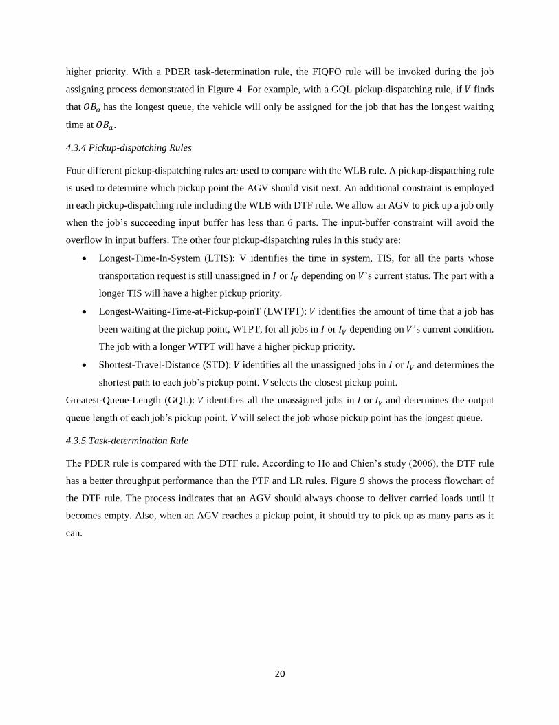
The PDER rule is compared with the DTF rule. According to Ho and Chien’s study (2006), the DTF rule
has a better throughput performance than the PTF and LR rules. Figure 9 shows the process flowchart of
the DTF rule. The process indicates that an AGV should always choose to deliver carried loads until it
becomes empty. Also, when an AGV reaches a pickup point, it should try to pick up as many parts as it
can.
21
Figure 9: DTF rule flowchart.
22
5. IMPLEMENTATION
Two simulation models were constructed using Simio simulation software version 9.147. We use six
modeling objects to build the hypothetical FMSs in Simio, including Source, Sink, Server, Modelentity,
Path, Vehicle, and Modelentity objects. The Source and Sink objects are the entry and exit of a system. A
Modelentity object is used as a part, which is created by a Source, processed by Servers, and destroyed by
a Sink. The Vehicle object is used to reproduce the behaviors of AGV that moves along the Paths. This
section explains the implementations of the PDER, DTF, and WLB rules in Simio.
5.1 Implementation of PDER
The Vehicle object in Simio 9.147 has the basic characteristics of a DTF task-determination rule. After a
Vehicle reaches an assigned output buffer, it will continue to load parts until all loading spaces are filled or
the output buffer becomes empty. Then, the Vehicle will continue to deliver the carried loads until it frees
up all loading spaces. In order to implement the PDER rule, the first step is to change the continue loading
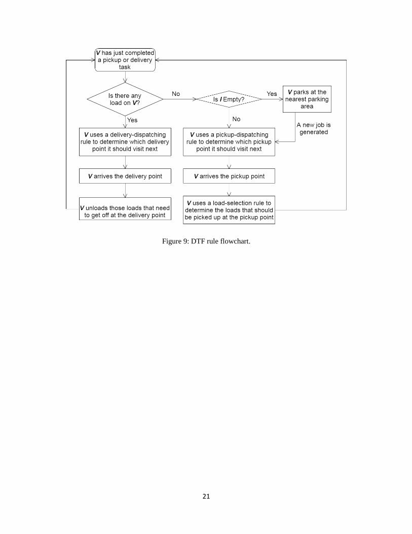
behavior. With a PDER rule, an AGV should only pick up the assigned job at a pickup point. Figure 10
demonstrates a portion of OnVisitingNode process for the Vehicle object in Simio. The OnVisitingNode
process is invoked whenever the Vehicle reaches a node (point). Figure 11 through 14 show the
modifications for the PDER rule. The blocks in gray are default steps. The block in green indicates that it
is a new or revised step. A block in red means it is a new or revised decision-making step. Each block in
yellow will invoke another process, which is demonstrated in the Appendix.
Figure 10: A portion of OnVisitingNode process for the Vehicle object in Simio.
23
Figure 11: Modification of Vehicle object that determines the next distance.
Figure 12: Modification of Vehicle object that assigns a job to empty AGV.
Figure 13: Modification of Vehicle object that determines low-cost-pickup-point and low-cost-job lists.
24
Figure 14: Modification of Vehicle object that assigns a low-cost job to AGV.
As shown in Figure 10, a Vehicle with original setup will first go through the NextDropoff step. If the
Vehicle is not empty, it will find the next delivery point based on a delivery-dispatching rule and then leave
the current location. If the Vehicle fails to find a part to deliver, it uses the NextPickup step to find the next
job to pick up among the assigned jobs. If there is no job assigned to the Vehicle, it will go through the
NewRequests step to find a new assignment based on a pickup-dispatching rule.
In the PDER setup, two local variables are used to record the closest pickup and delivery points for the
assigned and carried jobs. As shown in Figure 11, the ResetDropoffNode and RestpickupNode steps are
used to reset the variables. The NextDropoff and NextPickup steps will find the closest delivery and pickup
points. The AssigndropoffNode and AssignPickupNode steps assign the values of the variables to be the
closest pickup and delivery points. The IfFullyLoaded step examines if the AGV is fully loaded.
If the Vehicle fails to find a delivery point, the process will jump to the NextPickup step. If the Vehicle
is fully loaded, it will leave the current workstation and moves towards the closest delivery point (Case 3).
If the Vehicle fails to find neither a delivery point nor a pickup point, it indicates that the vehicle is empty
and unassigned (Case 1). The process will jump to the AssignPriority Step shown in Figure 12. The
AssignedPriority step assigns each job in the waiting list a priority based on a pickup-dispatching rule.
Notice that if the job’s succeeding input buffer has more than 6 parts waiting, the priority of the job becomes
0. The IfAllowPickup step examines if there is any part waiting in the system that can satisfy the input-
buffer constraint. If the waiting list is empty or no job can satisfy the constraint, the vehicle will park at the
current workstation. If there is at least one job that can satisfy the constraint, the job with the highest priority
will be assigned to the Vehicle through the NewRequests step.
If the Vehicle finds at least one pickup or delivery point, it will use the FindClosest step shown in
Figure 13 to find the closest destination. If there is not available pickup point, the closest destination will
be the closest delivery point and vice versa. Then, the IfFullyAssigned step examines if the total number of
assign and carried jobs equals the vehicle capacity. If the vehicle is fully assigned, it will move to the closest
25
destination (Case 3). Otherwise, the process moves to the ResetStarNode step. At this point, the AGV’s
current state should be partially loaded (Case 2). The ResetStarNode, FindEnRouteNode, IfStopSearching,
and ResetStarNode steps are used to define the low-cost-pickup-point list. The FindEnRoutePart step is
used to search and assign priorities to low-cost jobs based on a pickup-dispatching rule.
As shown in Figure 14, after assigning priorities to low-cost jobs, the Vehicle clears the low-cost-
pickup-point list through the RemoveEnRNode step. The AnyEnRouteJob and ResetEnroute steps are used
to examine the low-cost-job list. If the Vehicle fails to find any low cost job that can satisfy the constraint,
the Vehicle moves to the closest destination. Otherwise, the AssignLowCostJob step will assign the low-
cost job with the highest priority to the Vehicle. The reset step sets the priorities of all jobs in the system to
be 0. After that, the process moves back to the ResetDropOff step and starts over again.
Figure 15 demonstrates the process that makes the Vehicle object continuously load new parts when
arrives a pickup point in Simio 9.147. Figure 16 shows the modifications that change the continuous loading
behavior. As shown in Figure 15, the Rider, IfWaitUntilRiderLoad, and UntilRiderLoaded steps form a
loop process that as long as the Vehicle is not fully loaded and the output buffer is not empty, the Vehicle
will continue to pick up. As shown in Figure 16, we add the IfMoreAssignedJob process that will return
true only if another job in the current pickup point has been assigned to the Vehicle from a previous process.
The NumbOfLoad step is used to record the statistics of loading space utilization, which is irrelevant to the
continuous loading behavior.
Figure 15: A portion of OnVisitingNode process for the Vehicle object in Simio that cause the continuous
loading behavior.
26
Figure 16: Modification of Vehicle object that only allows the Vehicle to pick up assigned jobs.
5.2 Implementation of DTF
Although the default setup of a Vehicle object follows the DTF rule, some additional steps need to be added
to implement the pickup-dispatching rules and set the input-buffer constraint. Figure 17 and 18 demonstrate
the modifications for the Vehicle using DTF. As shown in Figure 17, the ResetContinue, DecideContinue
and IfContinue steps determine if the next part in the current output buffer can satisfy the input-buffer
constraint. If the constraint is satisfied, the IfCountinue step returns true and the Vehicle loads one more
part. Otherwise, the process moves to the IfMinimumDwell step. Again the NumberOfLoad step is used to
record the statistics of AGV capacity utilization.
Figure 17: Modification of Vehicle object that adds the input-buffer constrain.
27
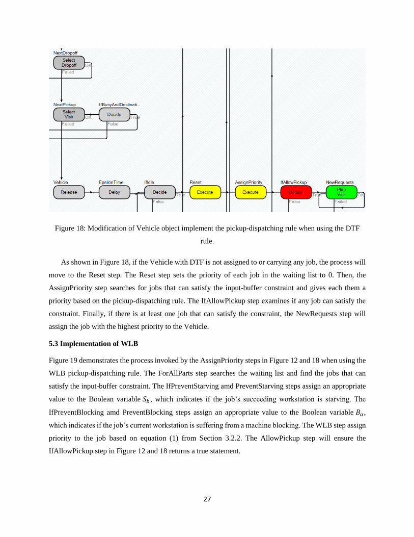
Figure 18: Modification of Vehicle object implement the pickup-dispatching rule when using the DTF
rule.
As shown in Figure 18, if the Vehicle with DTF is not assigned to or carrying any job, the process will
move to the Reset step. The Reset step sets the priority of each job in the waiting list to 0. Then, the
AssignPriority step searches for jobs that can satisfy the input-buffer constraint and gives each them a
priority based on the pickup-dispatching rule. The IfAllowPickup step examines if any job can satisfy the
constraint. Finally, if there is at least one job that can satisfy the constraint, the NewRequests step will
assign the job with the highest priority to the Vehicle.
5.3 Implementation of WLB
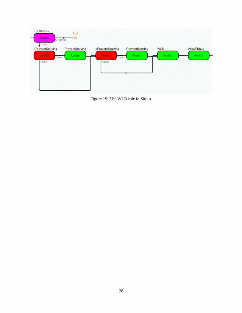
Figure 19 demonstrates the process invoked by the AssignPriority steps in Figure 12 and 18 when using the
WLB pickup-dispatching rule. The ForAllParts step searches the waiting list and find the jobs that can
satisfy the input-buffer constraint. The IfPreventStarving amd PreventStarving steps assign an appropriate
value to the Boolean variable 𝑆𝑏 , which indicates if the job’s succeeding workstation is starving. The
IfPreventBlocking amd PreventBlocking steps assign an appropriate value to the Boolean variable 𝐵𝑎 ,
which indicates if the job’s current workstation is suffering from a machine blocking. The WLB step assign
priority to the job based on equation (1) from Section 3.2.2. The AllowPickup step will ensure the
IfAllowPickup step in Figure 12 and 18 returns a true statement.
28
Figure 19: The WLB rule in Simio.
29
6. EXPERIMENT FOR THE PDER RULE
In this study, we conduct two simulation-based experiments. The first experiment (experiment 1) compares
the PDER rule with the DTF rule in two hypothetical FMSs. The second experiment (experiment 2)
compares the WLB rule with four pickup-dispatching rules while using both DTF and PDER task-
determination rules. This section presents the experiment design and output analysis of experiment 1.
6.1 Experiment Design (Experiment 1)
The first experiment compares the performance of the PDER and DTF task-selection rules paired with four
alternative pickup-dispatching rules in two FMS configurations, FMS 1 and FMS 2. The other factors under
consideration include the AGV fleet size ranging from 1 to 4 vehicles, and the vehicle types include dual-
and triple-load AGVs resulting in a total of 128 test scenarios. The experimental factors and their levels are
presented in Table 2. The primary performance measures considered for this experiment are throughput and
average time in system (ATIS).
Both FMS 1 and FMS 2 operate on a pull concept, that a new part with a random part type will enter
the system when the Entry station’s queue length is smaller than its capacity. The capacity of the Entry
station is 6 in both FMSs. In both configurations, an AGV’s loading and unloading times are 15 seconds
per part, and its travel speed is 2 miles per hour. The simulation experiments are set up to run 20 replication
of each scenario consisting of 500 hours of continuous operations which includes a warm-up period of 6
and 12 hours for FMS 1 and FMS 2, respectively.
Table 2: Factors considered in experiment 1.
Dispatching rules System Configuration
Pickup-
Dispatching
Task-
determination
Flexible manufacturing
system (FMS)
Number of AGV
(AGVs)
AGV Capacity
(AGV Cap.)
QGL PDER 1 1 2
LTIS DTF 2 2 3
LWTPT 3
STD 4
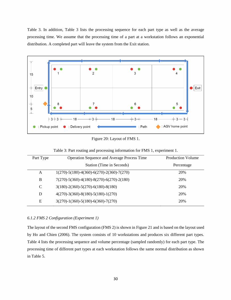
6.1.1 FMS 1 Configuration (Experiment 1)
The layout of the first FMS configuration (FMS 1) is shown in Figure 20. FMS 1 has a single-loop floor
layout, which consists of 8 workstations connected with unidirectional paths, and produces five part types.
The output buffer capacity of the Entry station is 6. After an AGV picks up a part from the output buffer, a
new part with random part type will flow into the system based on the production volume percentages in
30
Table 3. In addition, Table 3 lists the processing sequence for each part type as well as the average
processing time. We assume that the processing time of a part at a workstation follows an exponential
distribution. A completed part will leave the system from the Exit station.
Figure 20: Layout of FMS 1.
Table 3: Part routing and processing information for FMS 1, experiment 1.
Part Type
Operation Sequence and Average Process Time
Station (Time in Seconds)
Production Volume
Percentage
A 1(270)-5(180)-4(360)-6(270)-2(360)-7(270) 20%
B 7(270)-5(360)-4(180)-8(270)-6(270)-2(180) 20%
C 3(180)-2(360)-5(270)-6(180)-8(180) 20%
D 4(270)-3(360)-8(180)-5(180)-1(270) 20%
E 3(270)-1(360)-5(180)-6(360)-7(270) 20%
6.1.2 FMS 2 Configuration (Experiment 1)
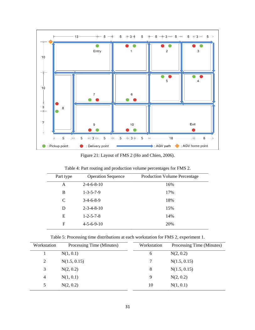
The layout of the second FMS configuration (FMS 2) is shown in Figure 21 and is based on the layout used
by Ho and Chien (2006). The system consists of 10 workstations and produces six different part types.
Table 4 lists the processing sequence and volume percentage (sampled randomly) for each part type. The
processing time of different part types at each workstation follows the same normal distribution as shown
in Table 5.
31
Figure 21: Layout of FMS 2 (Ho and Chien, 2006).
Table 4: Part routing and production volume percentages for FMS 2.
Part type Operation Sequence Production Volume Percentage
A 2-4-6-8-10 16%
B 1-3-5-7-9 17%
C 3-4-6-8-9 18%
D 2-3-4-8-10 15%
E 1-2-5-7-8 14%
F 4-5-6-9-10 20%
Table 5: Processing time distributions at each workstation for FMS 2, experiment 1.
Workstation Processing Time (Minutes) Workstation Processing Time (Minutes)
1 N(1, 0.1) 6 N(2, 0.2)
2 N(1.5, 0.15) 7 N(1.5, 0.15)
3 N(2, 0.2) 8 N(1.5, 0.15)
4 N(1, 0.1) 9 N(2, 0.2)
5 N(2, 0.2) 10 N(1, 0.1)
32
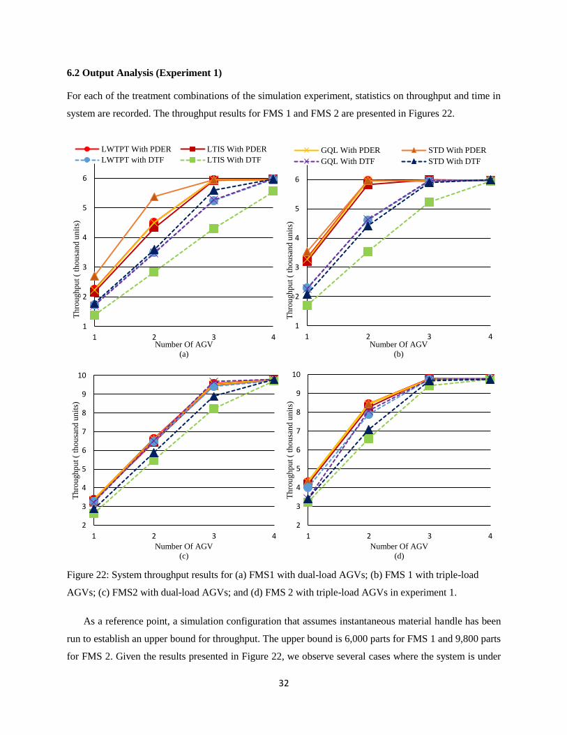
6.2 Output Analysis (Experiment 1)
For each of the treatment combinations of the simulation experiment, statistics on throughput and time in
system are recorded. The throughput results for FMS 1 and FMS 2 are presented in Figures 22.
Figure 22: System throughput results for (a) FMS1 with dual-load AGVs; (b) FMS 1 with triple-load
AGVs; (c) FMS2 with dual-load AGVs; and (d) FMS 2 with triple-load AGVs in experiment 1.
As a reference point, a simulation configuration that assumes instantaneous material handle has been
run to establish an upper bound for throughput. The upper bound is 6,000 parts for FMS 1 and 9,800 parts
for FMS 2. Given the results presented in Figure 22, we observe several cases where the system is under
1
2
3
4
5
6
1 2 3 4
Th
rou
gh
pu
t (
tho
usa
nd
un
its)
Number Of AGV
(a)
LWTPT With PDER LTIS With PDER
LWTPT with DTF LTIS With DTF
1
2
3
4
5
6
1 2 3 4
Th
rou
gh
pu
t (
tho
usa
nd
un
its)
Number Of AGV
(b)
GQL With PDER STD With PDER
GQL With DTF STD With DTF
2
3
4
5
6
7
8
9
10
1 2 3 4
Th
rou
gh
pu
t (
tho
usa
nd
un
its)
Number Of AGV
(c)
2
3
4
5
6
7
8
9
10
1 2 3 4
Th
rou
gh
pu
t (
tho
usa
nd
un
its)
Number Of AGV
(d)
33
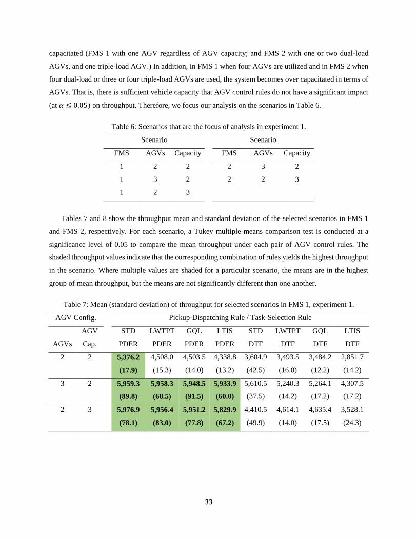
capacitated (FMS 1 with one AGV regardless of AGV capacity; and FMS 2 with one or two dual-load
AGVs, and one triple-load AGV.) In addition, in FMS 1 when four AGVs are utilized and in FMS 2 when
four dual-load or three or four triple-load AGVs are used, the system becomes over capacitated in terms of
AGVs. That is, there is sufficient vehicle capacity that AGV control rules do not have a significant impact
(at 𝛼 ≤ 0.05) on throughput. Therefore, we focus our analysis on the scenarios in Table 6.
Table 6: Scenarios that are the focus of analysis in experiment 1.
Scenario Scenario
FMS AGVs Capacity FMS AGVs Capacity
1 2 2 2 3 2
1 3 2 2 2 3
1 2 3
Tables 7 and 8 show the throughput mean and standard deviation of the selected scenarios in FMS 1
and FMS 2, respectively. For each scenario, a Tukey multiple-means comparison test is conducted at a
significance level of 0.05 to compare the mean throughput under each pair of AGV control rules. The
shaded throughput values indicate that the corresponding combination of rules yields the highest throughput
in the scenario. Where multiple values are shaded for a particular scenario, the means are in the highest
group of mean throughput, but the means are not significantly different than one another.
Table 7: Mean (standard deviation) of throughput for selected scenarios in FMS 1, experiment 1.
AGV Config. Pickup-Dispatching Rule / Task-Selection Rule
AGVs
AGV
Cap.
STD
PDER
LWTPT
PDER
GQL
PDER
LTIS
PDER
STD
DTF
LWTPT
DTF
GQL
DTF
LTIS
DTF
2 2 5,376.2 4,508.0 4,503.5 4,338.8 3,604.9 3,493.5 3,484.2 2,851.7
(17.9) (15.3) (14.0) (13.2) (42.5) (16.0) (12.2) (14.2)
3 2 5,959.3 5,958.3 5,948.5 5,933.9 5,610.5 5,240.3 5,264.1 4,307.5
(89.8) (68.5) (91.5) (60.0) (37.5) (14.2) (17.2) (17.2)
2 3 5,976.9 5,956.4 5,951.2 5,829.9 4,410.5 4,614.1 4,635.4 3,528.1
(78.1) (83.0) (77.8) (67.2) (49.9) (14.0) (17.5) (24.3)
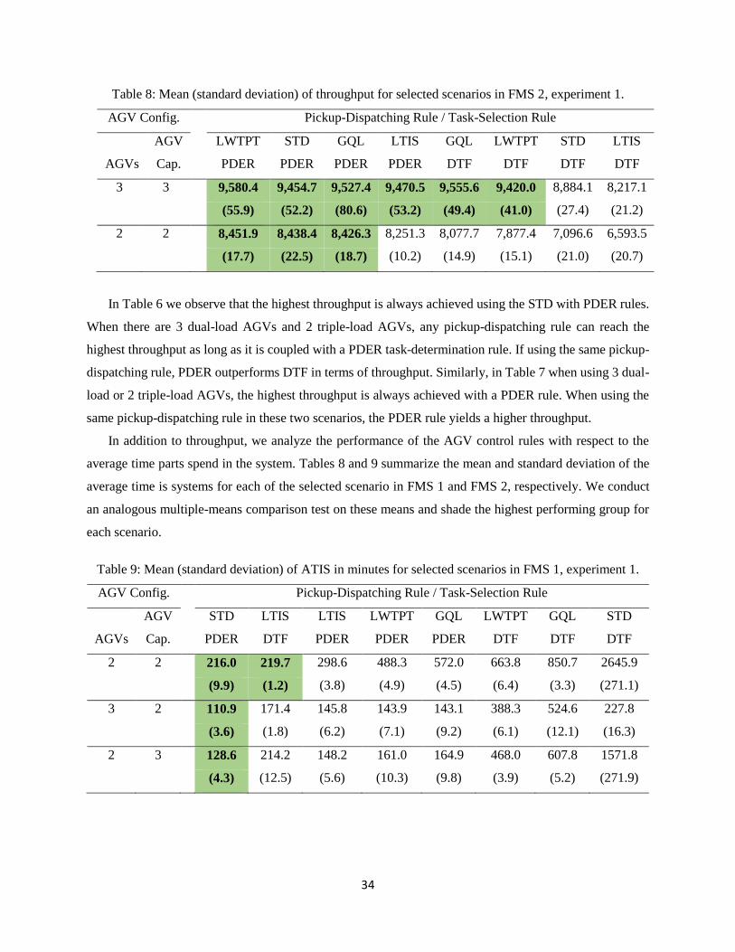
34
Table 8: Mean (standard deviation) of throughput for selected scenarios in FMS 2, experiment 1.
AGV Config. Pickup-Dispatching Rule / Task-Selection Rule
AGVs
AGV
Cap.
LWTPT
PDER
STD
PDER
GQL
PDER
LTIS
PDER
GQL
DTF
LWTPT
DTF
STD
DTF
LTIS
DTF
3 3 9,580.4 9,454.7 9,527.4 9,470.5 9,555.6 9,420.0 8,884.1 8,217.1
(55.9) (52.2) (80.6) (53.2) (49.4) (41.0) (27.4) (21.2)
2 2 8,451.9 8,438.4 8,426.3 8,251.3 8,077.7 7,877.4 7,096.6 6,593.5
(17.7) (22.5) (18.7) (10.2) (14.9) (15.1) (21.0) (20.7)
In Table 6 we observe that the highest throughput is always achieved using the STD with PDER rules.
When there are 3 dual-load AGVs and 2 triple-load AGVs, any pickup-dispatching rule can reach the
highest throughput as long as it is coupled with a PDER task-determination rule. If using the same pickup-
dispatching rule, PDER outperforms DTF in terms of throughput. Similarly, in Table 7 when using 3 dual-
load or 2 triple-load AGVs, the highest throughput is always achieved with a PDER rule. When using the
same pickup-dispatching rule in these two scenarios, the PDER rule yields a higher throughput.
In addition to throughput, we analyze the performance of the AGV control rules with respect to the
average time parts spend in the system. Tables 8 and 9 summarize the mean and standard deviation of the
average time is systems for each of the selected scenario in FMS 1 and FMS 2, respectively. We conduct
an analogous multiple-means comparison test on these means and shade the highest performing group for
each scenario.
Table 9: Mean (standard deviation) of ATIS in minutes for selected scenarios in FMS 1, experiment 1.
AGV Config. Pickup-Dispatching Rule / Task-Selection Rule
AGVs
AGV
Cap.
STD
PDER
LTIS
DTF
LTIS
PDER
LWTPT
PDER
GQL
PDER
LWTPT
DTF
GQL
DTF
STD
DTF
2 2 216.0 219.7 298.6 488.3 572.0 663.8 850.7 2645.9
(9.9) (1.2) (3.8) (4.9) (4.5) (6.4) (3.3) (271.1)
3 2 110.9 171.4 145.8 143.9 143.1 388.3 524.6 227.8
(3.6) (1.8) (6.2) (7.1) (9.2) (6.1) (12.1) (16.3)
2 3 128.6 214.2 148.2 161.0 164.9 468.0 607.8 1571.8
(4.3) (12.5) (5.6) (10.3) (9.8) (3.9) (5.2) (271.9)
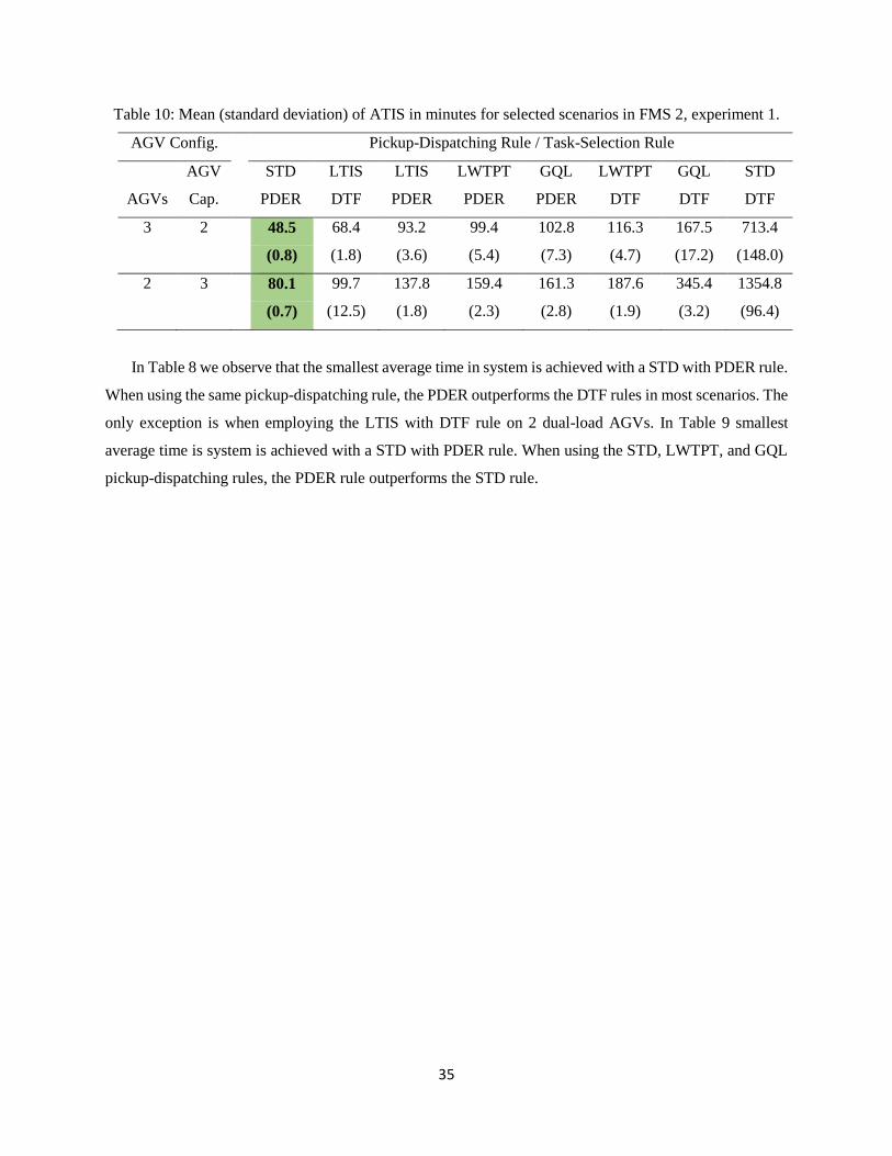
35
Table 10: Mean (standard deviation) of ATIS in minutes for selected scenarios in FMS 2, experiment 1.
AGV Config. Pickup-Dispatching Rule / Task-Selection Rule
AGVs
AGV
Cap.
STD
PDER
LTIS
DTF
LTIS
PDER
LWTPT
PDER
GQL
PDER
LWTPT
DTF
GQL
DTF
STD
DTF
3 2 48.5 68.4 93.2 99.4 102.8 116.3 167.5 713.4
(0.8) (1.8) (3.6) (5.4) (7.3) (4.7) (17.2) (148.0)
2 3 80.1 99.7 137.8 159.4 161.3 187.6 345.4 1354.8
(0.7) (12.5) (1.8) (2.3) (2.8) (1.9) (3.2) (96.4)
In Table 8 we observe that the smallest average time in system is achieved with a STD with PDER rule.
When using the same pickup-dispatching rule, the PDER outperforms the DTF rules in most scenarios. The
only exception is when employing the LTIS with DTF rule on 2 dual-load AGVs. In Table 9 smallest
average time is system is achieved with a STD with PDER rule. When using the STD, LWTPT, and GQL
pickup-dispatching rules, the PDER rule outperforms the STD rule.
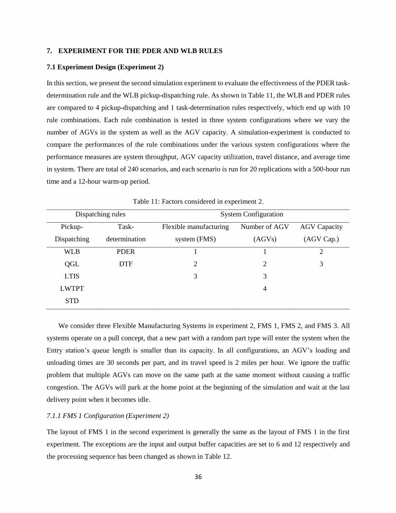
36
7. EXPERIMENT FOR THE PDER AND WLB RULES
7.1 Experiment Design (Experiment 2)
In this section, we present the second simulation experiment to evaluate the effectiveness of the PDER task-
determination rule and the WLB pickup-dispatching rule. As shown in Table 11, the WLB and PDER rules
are compared to 4 pickup-dispatching and 1 task-determination rules respectively, which end up with 10
rule combinations. Each rule combination is tested in three system configurations where we vary the
number of AGVs in the system as well as the AGV capacity. A simulation-experiment is conducted to
compare the performances of the rule combinations under the various system configurations where the
performance measures are system throughput, AGV capacity utilization, travel distance, and average time
in system. There are total of 240 scenarios, and each scenario is run for 20 replications with a 500-hour run
time and a 12-hour warm-up period.
Table 11: Factors considered in experiment 2.
Dispatching rules System Configuration
Pickup-
Dispatching
Task-
determination
Flexible manufacturing
system (FMS)
Number of AGV
(AGVs)
AGV Capacity
(AGV Cap.)
WLB PDER 1 1 2
QGL DTF 2 2 3
LTIS 3 3
LWTPT 4
STD
We consider three Flexible Manufacturing Systems in experiment 2, FMS 1, FMS 2, and FMS 3. All
systems operate on a pull concept, that a new part with a random part type will enter the system when the
Entry station’s queue length is smaller than its capacity. In all configurations, an AGV’s loading and
unloading times are 30 seconds per part, and its travel speed is 2 miles per hour. We ignore the traffic
problem that multiple AGVs can move on the same path at the same moment without causing a traffic
congestion. The AGVs will park at the home point at the beginning of the simulation and wait at the last
delivery point when it becomes idle.
7.1.1 FMS 1 Configuration (Experiment 2)
The layout of FMS 1 in the second experiment is generally the same as the layout of FMS 1 in the first
experiment. The exceptions are the input and output buffer capacities are set to 6 and 12 respectively and
the processing sequence has been changed as shown in Table 12.
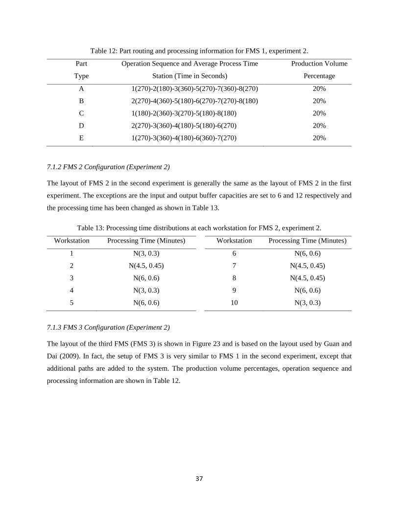
37
Table 12: Part routing and processing information for FMS 1, experiment 2.
Part
Type
Operation Sequence and Average Process Time
Station (Time in Seconds)
Production Volume
Percentage
A 1(270)-2(180)-3(360)-5(270)-7(360)-8(270) 20%
B 2(270)-4(360)-5(180)-6(270)-7(270)-8(180) 20%
C 1(180)-2(360)-3(270)-5(180)-8(180) 20%
D 2(270)-3(360)-4(180)-5(180)-6(270) 20%
E 1(270)-3(360)-4(180)-6(360)-7(270) 20%
7.1.2 FMS 2 Configuration (Experiment 2)
The layout of FMS 2 in the second experiment is generally the same as the layout of FMS 2 in the first
experiment. The exceptions are the input and output buffer capacities are set to 6 and 12 respectively and
the processing time has been changed as shown in Table 13.
Table 13: Processing time distributions at each workstation for FMS 2, experiment 2.
Workstation Processing Time (Minutes) Workstation Processing Time (Minutes)
1 N(3, 0.3) 6 N(6, 0.6)
2 N(4.5, 0.45) 7 N(4.5, 0.45)
3 N(6, 0.6) 8 N(4.5, 0.45)
4 N(3, 0.3) 9 N(6, 0.6)
5 N(6, 0.6) 10 N(3, 0.3)
7.1.3 FMS 3 Configuration (Experiment 2)
The layout of the third FMS (FMS 3) is shown in Figure 23 and is based on the layout used by Guan and
Dai (2009). In fact, the setup of FMS 3 is very similar to FMS 1 in the second experiment, except that
additional paths are added to the system. The production volume percentages, operation sequence and
processing information are shown in Table 12.
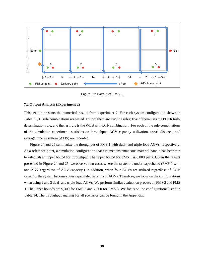
38
Figure 23: Layout of FMS 3.
7.2 Output Analysis (Experiment 2)
This section presents the numerical results from experiment 2. For each system configuration shown in
Table 11, 10 rule combinations are tested. Four of them are existing rules; five of them uses the PDER task-
determination rule; and the last rule is the WLB with DTF combination. For each of the rule combinations
of the simulation experiment, statistics on throughput, AGV capacity utilization, travel distance, and
average time in system (ATIS) are recorded.
Figure 24 and 25 summarize the throughput of FMS 1 with dual- and triple-load AGVs, respectively.
As a reference point, a simulation configuration that assumes instantaneous material handle has been run
to establish an upper bound for throughput. The upper bound for FMS 1 is 6,800 parts. Given the results
presented in Figure 24 and 25, we observe two cases where the system is under capacitated (FMS 1 with
one AGV regardless of AGV capacity.) In addition, when four AGVs are utilized regardless of AGV
capacity, the system becomes over capacitated in terms of AGVs. Therefore, we focus on the configurations
when using 2 and 3 dual- and triple-load AGVs. We perform similar evaluation process on FMS 2 and FMS
3. The upper bounds are 9,300 for FMS 2 and 7,000 for FMS 3. We focus on the configurations listed in
Table 14. The throughput analysis for all scenarios can be found in the Appendix.
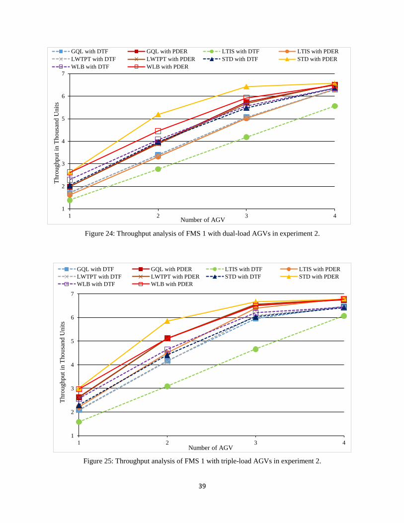
39
Figure 24: Throughput analysis of FMS 1 with dual-load AGVs in experiment 2.
Figure 25: Throughput analysis of FMS 1 with triple-load AGVs in experiment 2.
1
2
3
4
5
6
7
1 2 3 4
Thro
ughp
ut
in T
ho
usa
nd
Unit
s
Number of AGV
GQL with DTF GQL with PDER LTIS with DTF LTIS with PDER
LWTPT with DTF LWTPT with PDER STD with DTF STD with PDER
WLB with DTF WLB with PDER
1
2
3
4
5
6
7
1 2 3 4
Thro
ughp
ut
in T
ho
usa
nd
Unit
s
Number of AGV
GQL with DTF GQL with PDER LTIS with DTF LTIS with PDER
LWTPT with DTF LWTPT with PDER STD with DTF STD with PDER
WLB with DTF WLB with PDER
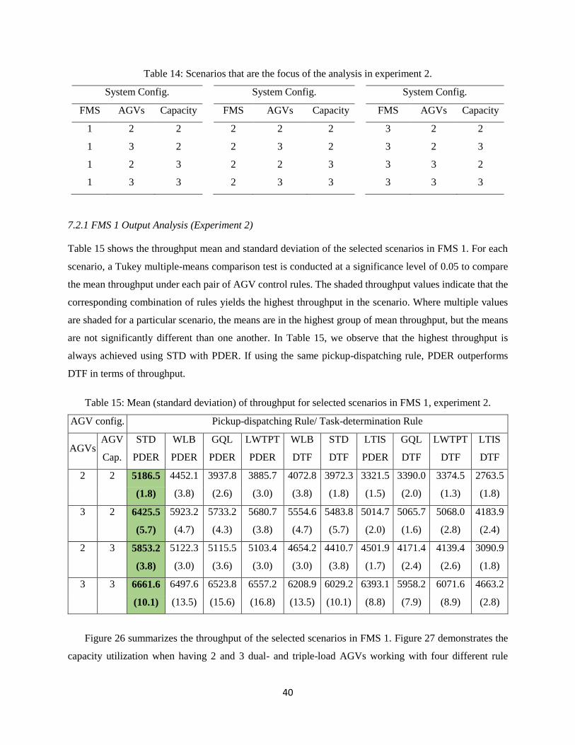
40
Table 14: Scenarios that are the focus of the analysis in experiment 2.
System Config. System Config. System Config.
FMS AGVs Capacity FMS AGVs Capacity FMS AGVs Capacity
1 2 2 2 2 2 3 2 2
1 3 2 2 3 2 3 2 3
1 2 3 2 2 3 3 3 2
1 3 3 2 3 3 3 3 3
7.2.1 FMS 1 Output Analysis (Experiment 2)
Table 15 shows the throughput mean and standard deviation of the selected scenarios in FMS 1. For each
scenario, a Tukey multiple-means comparison test is conducted at a significance level of 0.05 to compare
the mean throughput under each pair of AGV control rules. The shaded throughput values indicate that the
corresponding combination of rules yields the highest throughput in the scenario. Where multiple values
are shaded for a particular scenario, the means are in the highest group of mean throughput, but the means
are not significantly different than one another. In Table 15, we observe that the highest throughput is
always achieved using STD with PDER. If using the same pickup-dispatching rule, PDER outperforms
DTF in terms of throughput.
Table 15: Mean (standard deviation) of throughput for selected scenarios in FMS 1, experiment 2.
AGV config. Pickup-dispatching Rule/ Task-determination Rule
AGVs AGV
Cap.
STD
PDER
WLB
PDER
GQL
PDER
LWTPT
PDER
WLB
DTF
STD
DTF
LTIS
PDER
GQL
DTF
LWTPT
DTF
LTIS
DTF
2 2 5186.5 4452.1 3937.8 3885.7 4072.8 3972.3 3321.5 3390.0 3374.5 2763.5
(1.8) (3.8) (2.6) (3.0) (3.8) (1.8) (1.5) (2.0) (1.3) (1.8)
3 2 6425.5 5923.2 5733.2 5680.7 5554.6 5483.8 5014.7 5065.7 5068.0 4183.9
(5.7) (4.7) (4.3) (3.8) (4.7) (5.7) (2.0) (1.6) (2.8) (2.4)
2 3 5853.2 5122.3 5115.5 5103.4 4654.2 4410.7 4501.9 4171.4 4139.4 3090.9
(3.8) (3.0) (3.6) (3.0) (3.0) (3.8) (1.7) (2.4) (2.6) (1.8)
3 3 6661.6 6497.6 6523.8 6557.2 6208.9 6029.2 6393.1 5958.2 6071.6 4663.2
(10.1) (13.5) (15.6) (16.8) (13.5) (10.1) (8.8) (7.9) (8.9) (2.8)
Figure 26 summarizes the throughput of the selected scenarios in FMS 1. Figure 27 demonstrates the
capacity utilization when having 2 and 3 dual- and triple-load AGVs working with four different rule
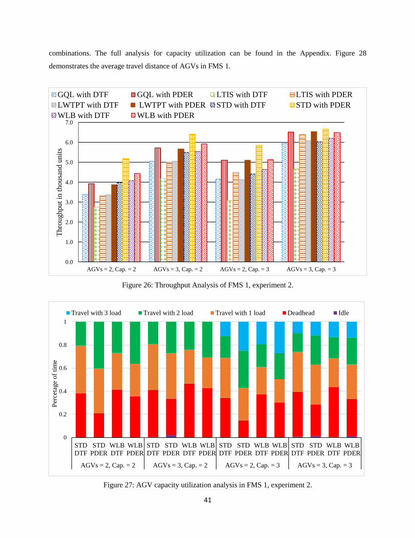
41
combinations. The full analysis for capacity utilization can be found in the Appendix. Figure 28
demonstrates the average travel distance of AGVs in FMS 1.
Figure 26: Throughput Analysis of FMS 1, experiment 2.
Figure 27: AGV capacity utilization analysis in FMS 1, experiment 2.
0.0
1.0
2.0
3.0
4.0
5.0
6.0
7.0
AGVs = 2, Cap. = 2 AGVs = 3, Cap. = 2 AGVs = 2, Cap. = 3 AGVs = 3, Cap. = 3
Thro
ughput
in t
ho
usa
nd
un
its
GQL with DTF GQL with PDER LTIS with DTF LTIS with PDER
LWTPT with DTF LWTPT with PDER STD with DTF STD with PDER
WLB with DTF WLB with PDER
0
0.2
0.4
0.6
0.8
1
STD
DTF
STD
PDER
WLB
DTF
WLB
PDER
STD
DTF
STD
PDER
WLB
DTF
WLB
PDER
STD
DTF
STD
PDER
WLB
DTF
WLB
PDER
STD
DTF
STD
PDER
WLB
DTF
WLB
PDER
AGVs = 2, Cap. = 2 AGVs = 3, Cap. = 2 AGVs = 2, Cap. = 3 AGVs = 3, Cap. = 3
Per
ceta
ge
of
tim
e
Travel with 3 load Travel with 2 load Travel with 1 load Deadhead Idle
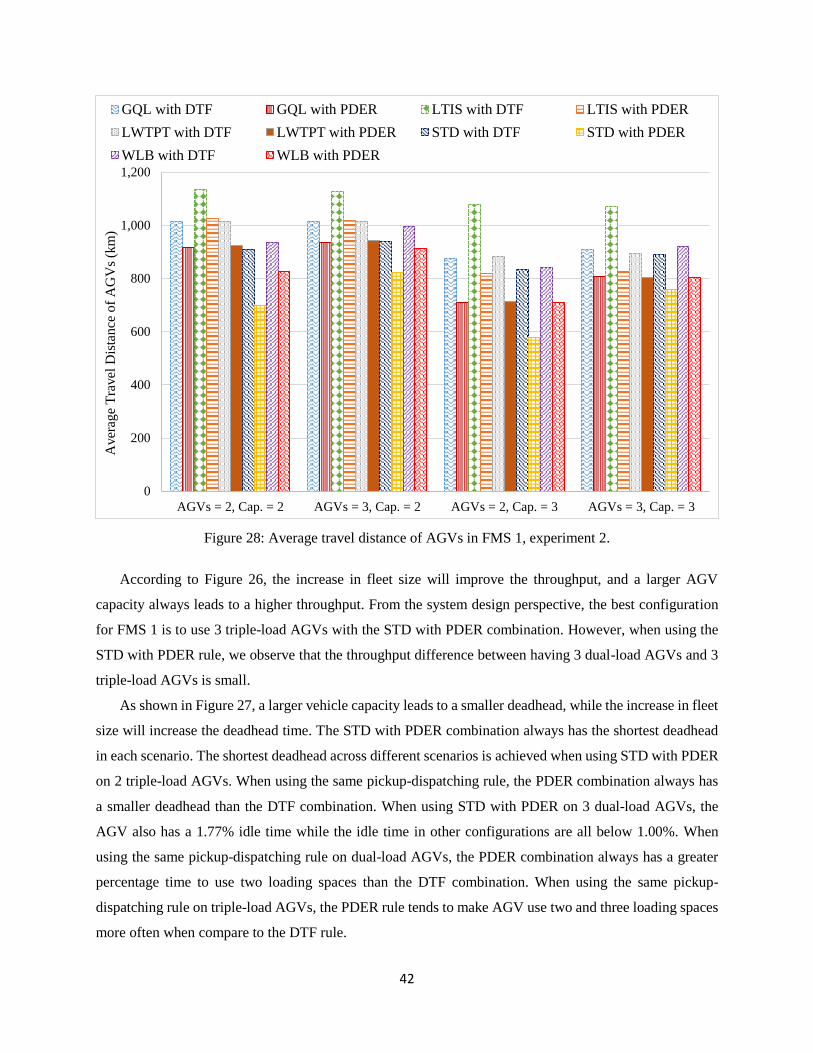
42
Figure 28: Average travel distance of AGVs in FMS 1, experiment 2.
According to Figure 26, the increase in fleet size will improve the throughput, and a larger AGV
capacity always leads to a higher throughput. From the system design perspective, the best configuration
for FMS 1 is to use 3 triple-load AGVs with the STD with PDER combination. However, when using the
STD with PDER rule, we observe that the throughput difference between having 3 dual-load AGVs and 3
triple-load AGVs is small.
As shown in Figure 27, a larger vehicle capacity leads to a smaller deadhead, while the increase in fleet
size will increase the deadhead time. The STD with PDER combination always has the shortest deadhead
in each scenario. The shortest deadhead across different scenarios is achieved when using STD with PDER
on 2 triple-load AGVs. When using the same pickup-dispatching rule, the PDER combination always has
a smaller deadhead than the DTF combination. When using STD with PDER on 3 dual-load AGVs, the
AGV also has a 1.77% idle time while the idle time in other configurations are all below 1.00%. When
using the same pickup-dispatching rule on dual-load AGVs, the PDER combination always has a greater
percentage time to use two loading spaces than the DTF combination. When using the same pickup-
dispatching rule on triple-load AGVs, the PDER rule tends to make AGV use two and three loading spaces
more often when compare to the DTF rule.
0
200
400
600
800
1,000
1,200
AGVs = 2, Cap. = 2 AGVs = 3, Cap. = 2 AGVs = 2, Cap. = 3 AGVs = 3, Cap. = 3
Aver
age
Tra
vel
Dis
tan
ce o
f A
GV
s (k
m)
GQL with DTF GQL with PDER LTIS with DTF LTIS with PDER
LWTPT with DTF LWTPT with PDER STD with DTF STD with PDER
WLB with DTF WLB with PDER
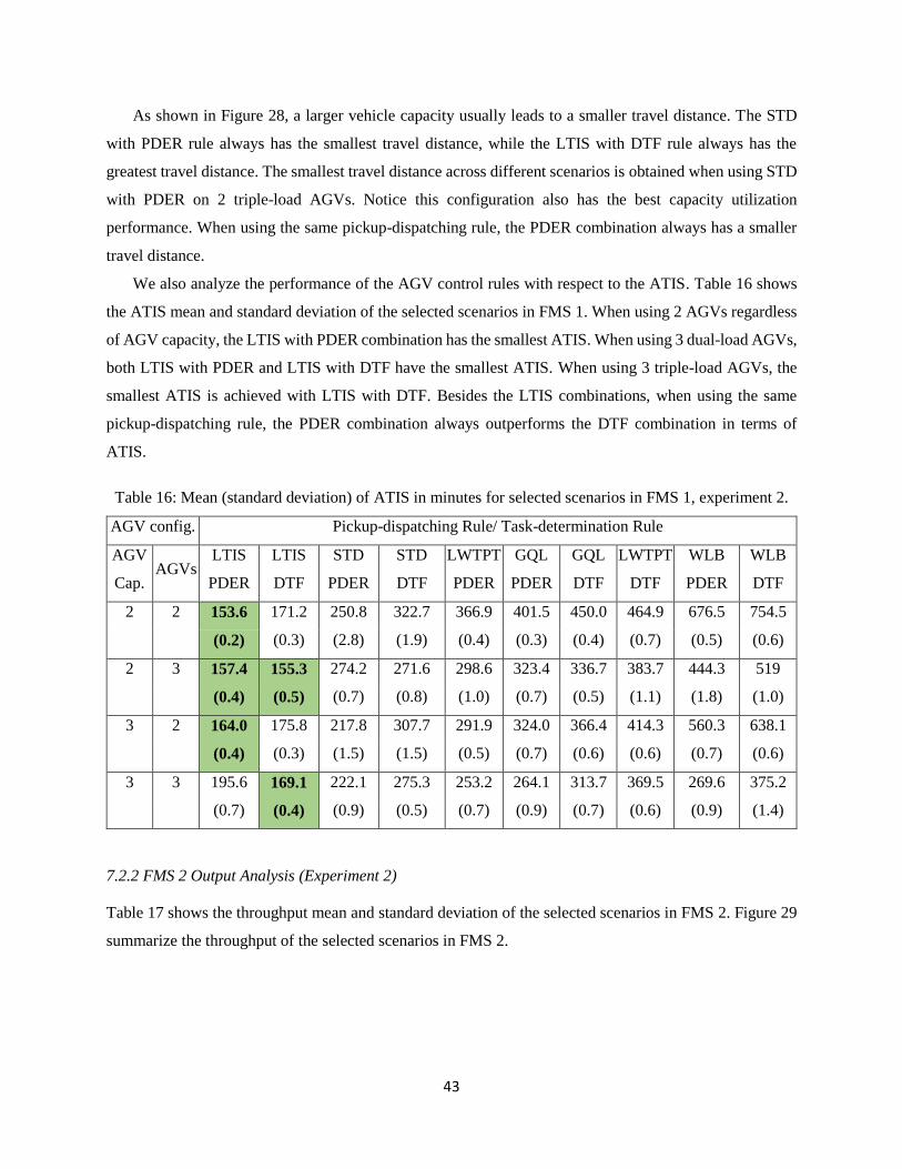
43
As shown in Figure 28, a larger vehicle capacity usually leads to a smaller travel distance. The STD
with PDER rule always has the smallest travel distance, while the LTIS with DTF rule always has the
greatest travel distance. The smallest travel distance across different scenarios is obtained when using STD
with PDER on 2 triple-load AGVs. Notice this configuration also has the best capacity utilization
performance. When using the same pickup-dispatching rule, the PDER combination always has a smaller
travel distance.
We also analyze the performance of the AGV control rules with respect to the ATIS. Table 16 shows
the ATIS mean and standard deviation of the selected scenarios in FMS 1. When using 2 AGVs regardless
of AGV capacity, the LTIS with PDER combination has the smallest ATIS. When using 3 dual-load AGVs,
both LTIS with PDER and LTIS with DTF have the smallest ATIS. When using 3 triple-load AGVs, the
smallest ATIS is achieved with LTIS with DTF. Besides the LTIS combinations, when using the same
pickup-dispatching rule, the PDER combination always outperforms the DTF combination in terms of
ATIS.
Table 16: Mean (standard deviation) of ATIS in minutes for selected scenarios in FMS 1, experiment 2.
AGV config. Pickup-dispatching Rule/ Task-determination Rule
AGV
Cap. AGVs
LTIS
PDER
LTIS
DTF
STD
PDER
STD
DTF
LWTPT
PDER
GQL
PDER
GQL
DTF
LWTPT
DTF
WLB
PDER
WLB
DTF
2 2 153.6 171.2 250.8 322.7 366.9 401.5 450.0 464.9 676.5 754.5
(0.2) (0.3) (2.8) (1.9) (0.4) (0.3) (0.4) (0.7) (0.5) (0.6)
2 3 157.4 155.3 274.2 271.6 298.6 323.4 336.7 383.7 444.3 519
(0.4) (0.5) (0.7) (0.8) (1.0) (0.7) (0.5) (1.1) (1.8) (1.0)
3 2 164.0 175.8 217.8 307.7 291.9 324.0 366.4 414.3 560.3 638.1
(0.4) (0.3) (1.5) (1.5) (0.5) (0.7) (0.6) (0.6) (0.7) (0.6)
3 3 195.6 169.1 222.1 275.3 253.2 264.1 313.7 369.5 269.6 375.2
(0.7) (0.4) (0.9) (0.5) (0.7) (0.9) (0.7) (0.6) (0.9) (1.4)
7.2.2 FMS 2 Output Analysis (Experiment 2)
Table 17 shows the throughput mean and standard deviation of the selected scenarios in FMS 2. Figure 29
summarize the throughput of the selected scenarios in FMS 2.
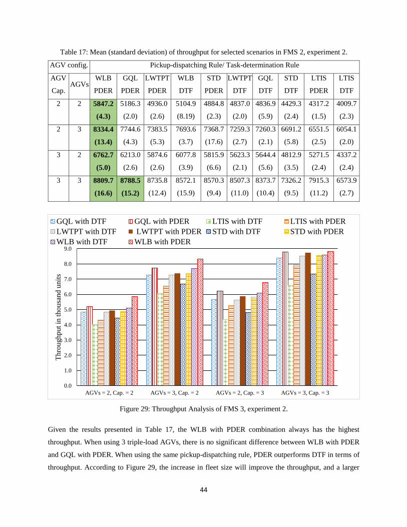
44
Table 17: Mean (standard deviation) of throughput for selected scenarios in FMS 2, experiment 2.
AGV config. Pickup-dispatching Rule/ Task-determination Rule
AGV
Cap. AGVs
WLB
PDER
GQL
PDER
LWTPT
PDER
WLB
DTF
STD
PDER
LWTPT
DTF
GQL
DTF
STD
DTF
LTIS
PDER
LTIS
DTF
2 2 5847.2 5186.3 4936.0 5104.9 4884.8 4837.0 4836.9 4429.3 4317.2 4009.7
(4.3) (2.0) (2.6) (8.19) (2.3) (2.0) (5.9) (2.4) (1.5) (2.3)
2 3 8334.4 7744.6 7383.5 7693.6 7368.7 7259.3 7260.3 6691.2 6551.5 6054.1
(13.4) (4.3) (5.3) (3.7) (17.6) (2.7) (2.1) (5.8) (2.5) (2.0)
3 2 6762.7 6213.0 5874.6 6077.8 5815.9 5623.3 5644.4 4812.9 5271.5 4337.2
(5.0) (2.6) (2.6) (3.9) (6.6) (2.1) (5.6) (3.5) (2.4) (2.4)
3 3 8809.7 8788.5 8735.8 8572.1 8570.3 8507.3 8373.7 7326.2 7915.3 6573.9
(16.6) (15.2) (12.4) (15.9) (9.4) (11.0) (10.4) (9.5) (11.2) (2.7)
Figure 29: Throughput Analysis of FMS 3, experiment 2.
Given the results presented in Table 17, the WLB with PDER combination always has the highest
throughput. When using 3 triple-load AGVs, there is no significant difference between WLB with PDER
and GQL with PDER. When using the same pickup-dispatching rule, PDER outperforms DTF in terms of
throughput. According to Figure 29, the increase in fleet size will improve the throughput, and a larger
0.0
1.0
2.0
3.0
4.0
5.0
6.0
7.0
8.0
9.0
AGVs = 2, Cap. = 2 AGVs = 3, Cap. = 2 AGVs = 2, Cap. = 3 AGVs = 3, Cap. = 3
Thro
ughput
in t
housa
nd u
nit
s
GQL with DTF GQL with PDER LTIS with DTF LTIS with PDER
LWTPT with DTF LWTPT with PDER STD with DTF STD with PDER
WLB with DTF WLB with PDER
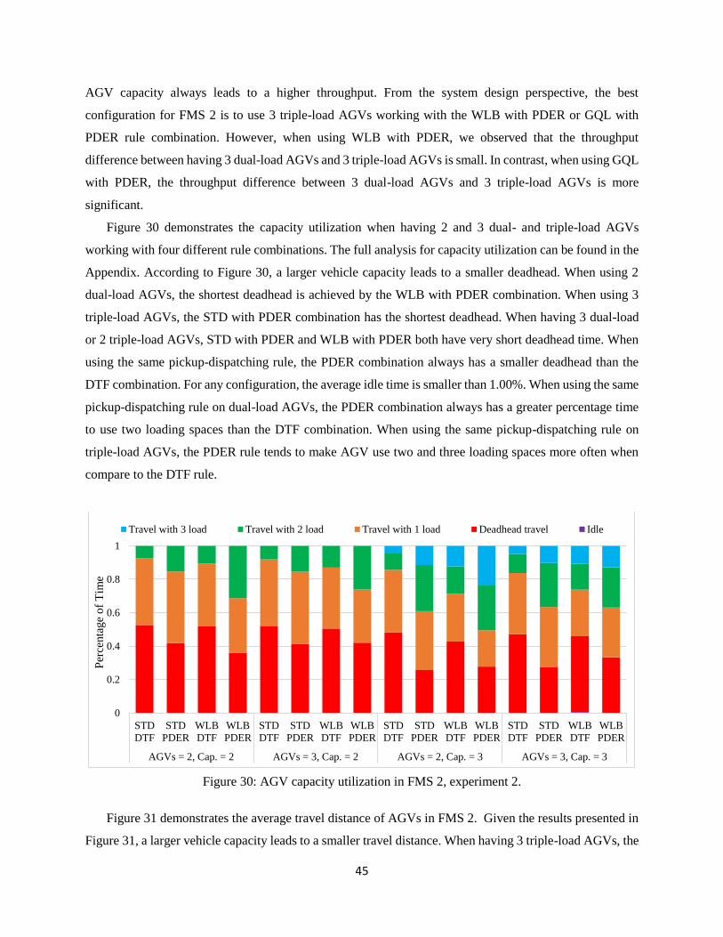
45
AGV capacity always leads to a higher throughput. From the system design perspective, the best
configuration for FMS 2 is to use 3 triple-load AGVs working with the WLB with PDER or GQL with
PDER rule combination. However, when using WLB with PDER, we observed that the throughput
difference between having 3 dual-load AGVs and 3 triple-load AGVs is small. In contrast, when using GQL
with PDER, the throughput difference between 3 dual-load AGVs and 3 triple-load AGVs is more
significant.
Figure 30 demonstrates the capacity utilization when having 2 and 3 dual- and triple-load AGVs
working with four different rule combinations. The full analysis for capacity utilization can be found in the
Appendix. According to Figure 30, a larger vehicle capacity leads to a smaller deadhead. When using 2
dual-load AGVs, the shortest deadhead is achieved by the WLB with PDER combination. When using 3
triple-load AGVs, the STD with PDER combination has the shortest deadhead. When having 3 dual-load
or 2 triple-load AGVs, STD with PDER and WLB with PDER both have very short deadhead time. When
using the same pickup-dispatching rule, the PDER combination always has a smaller deadhead than the
DTF combination. For any configuration, the average idle time is smaller than 1.00%. When using the same
pickup-dispatching rule on dual-load AGVs, the PDER combination always has a greater percentage time
to use two loading spaces than the DTF combination. When using the same pickup-dispatching rule on
triple-load AGVs, the PDER rule tends to make AGV use two and three loading spaces more often when
compare to the DTF rule.
Figure 30: AGV capacity utilization in FMS 2, experiment 2.
Figure 31 demonstrates the average travel distance of AGVs in FMS 2. Given the results presented in
Figure 31, a larger vehicle capacity leads to a smaller travel distance. When having 3 triple-load AGVs, the
0
0.2
0.4
0.6
0.8
1
STD
DTF
STD
PDER
WLB
DTF
WLB
PDER
STD
DTF
STD
PDER
WLB
DTF
WLB
PDER
STD
DTF
STD
PDER
WLB
DTF
WLB
PDER
STD
DTF
STD
PDER
WLB
DTF
WLB
PDER
AGVs = 2, Cap. = 2 AGVs = 3, Cap. = 2 AGVs = 2, Cap. = 3 AGVs = 3, Cap. = 3
Per
centa
ge
of
Tim
e
Travel with 3 load Travel with 2 load Travel with 1 load Deadhead travel Idle
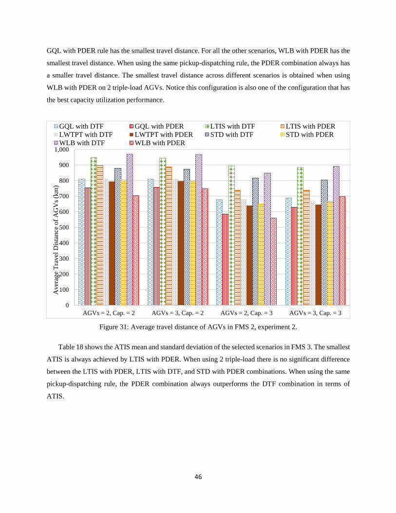
46
GQL with PDER rule has the smallest travel distance. For all the other scenarios, WLB with PDER has the
smallest travel distance. When using the same pickup-dispatching rule, the PDER combination always has
a smaller travel distance. The smallest travel distance across different scenarios is obtained when using
WLB with PDER on 2 triple-load AGVs. Notice this configuration is also one of the configuration that has
the best capacity utilization performance.
Figure 31: Average travel distance of AGVs in FMS 2, experiment 2.
Table 18 shows the ATIS mean and standard deviation of the selected scenarios in FMS 3. The smallest
ATIS is always achieved by LTIS with PDER. When using 2 triple-load there is no significant difference
between the LTIS with PDER, LTIS with DTF, and STD with PDER combinations. When using the same
pickup-dispatching rule, the PDER combination always outperforms the DTF combination in terms of
ATIS.
0
100
200
300
400
500
600
700
800
900
1,000
AGVs = 2, Cap. = 2 AGVs = 3, Cap. = 2 AGVs = 2, Cap. = 3 AGVs = 3, Cap. = 3
Aver
age
Tra
vel
Dis
tance
of
AG
Vs
(km
)
GQL with DTF GQL with PDER LTIS with DTF LTIS with PDER
LWTPT with DTF LWTPT with PDER STD with DTF STD with PDER
WLB with DTF WLB with PDER
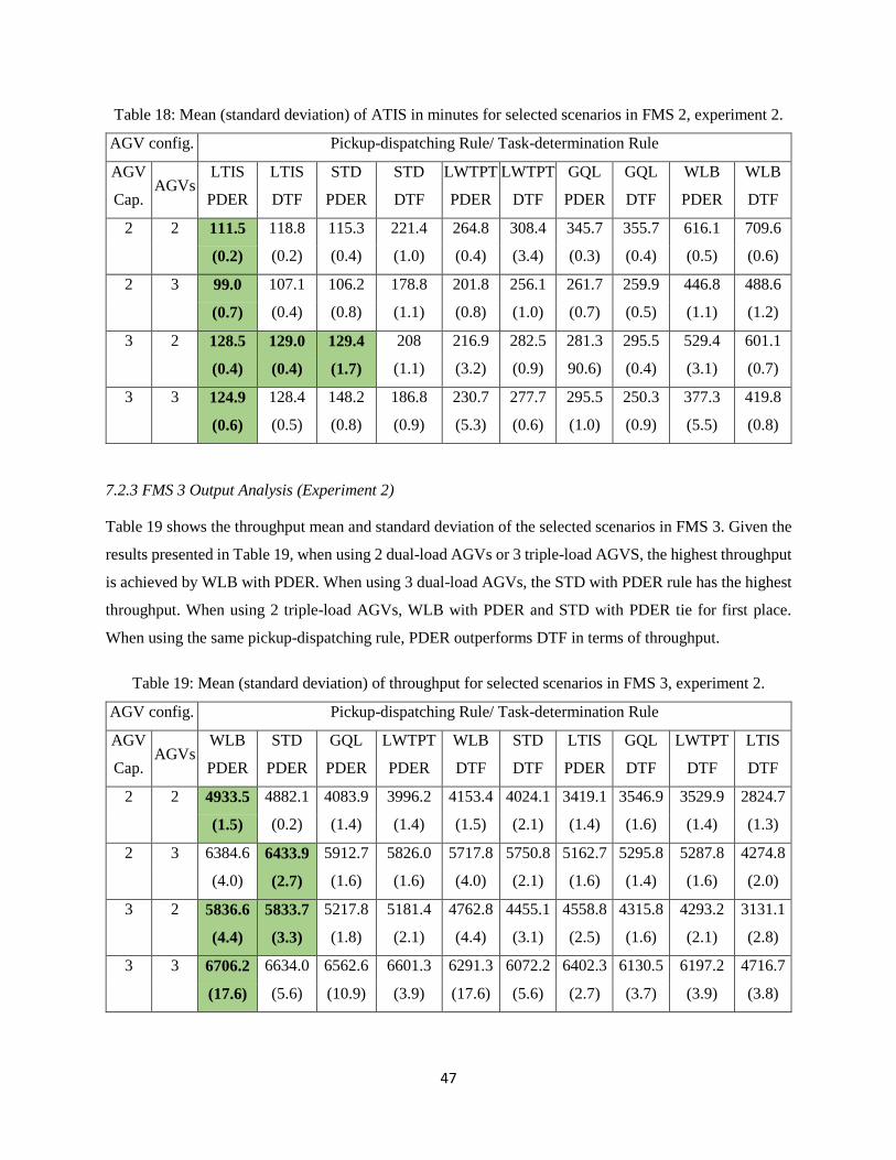
47
Table 18: Mean (standard deviation) of ATIS in minutes for selected scenarios in FMS 2, experiment 2.
AGV config. Pickup-dispatching Rule/ Task-determination Rule
AGV
Cap. AGVs
LTIS
PDER
LTIS
DTF
STD
PDER
STD
DTF
LWTPT
PDER
LWTPT
DTF
GQL
PDER
GQL
DTF
WLB
PDER
WLB
DTF
2 2 111.5 118.8 115.3 221.4 264.8 308.4 345.7 355.7 616.1 709.6
(0.2) (0.2) (0.4) (1.0) (0.4) (3.4) (0.3) (0.4) (0.5) (0.6)
2 3 99.0 107.1 106.2 178.8 201.8 256.1 261.7 259.9 446.8 488.6
(0.7) (0.4) (0.8) (1.1) (0.8) (1.0) (0.7) (0.5) (1.1) (1.2)
3 2 128.5 129.0 129.4 208 216.9 282.5 281.3 295.5 529.4 601.1
(0.4) (0.4) (1.7) (1.1) (3.2) (0.9) 90.6) (0.4) (3.1) (0.7)
3 3 124.9 128.4 148.2 186.8 230.7 277.7 295.5 250.3 377.3 419.8
(0.6) (0.5) (0.8) (0.9) (5.3) (0.6) (1.0) (0.9) (5.5) (0.8)
7.2.3 FMS 3 Output Analysis (Experiment 2)
Table 19 shows the throughput mean and standard deviation of the selected scenarios in FMS 3. Given the
results presented in Table 19, when using 2 dual-load AGVs or 3 triple-load AGVS, the highest throughput
is achieved by WLB with PDER. When using 3 dual-load AGVs, the STD with PDER rule has the highest
throughput. When using 2 triple-load AGVs, WLB with PDER and STD with PDER tie for first place.
When using the same pickup-dispatching rule, PDER outperforms DTF in terms of throughput.
Table 19: Mean (standard deviation) of throughput for selected scenarios in FMS 3, experiment 2.
AGV config. Pickup-dispatching Rule/ Task-determination Rule
AGV
Cap. AGVs
WLB
PDER
STD
PDER
GQL
PDER
LWTPT
PDER
WLB
DTF
STD
DTF
LTIS
PDER
GQL
DTF
LWTPT
DTF
LTIS
DTF
2 2 4933.5 4882.1 4083.9 3996.2 4153.4 4024.1 3419.1 3546.9 3529.9 2824.7
(1.5) (0.2) (1.4) (1.4) (1.5) (2.1) (1.4) (1.6) (1.4) (1.3)
2 3 6384.6 6433.9 5912.7 5826.0 5717.8 5750.8 5162.7 5295.8 5287.8 4274.8
(4.0) (2.7) (1.6) (1.6) (4.0) (2.1) (1.6) (1.4) (1.6) (2.0)
3 2 5836.6 5833.7 5217.8 5181.4 4762.8 4455.1 4558.8 4315.8 4293.2 3131.1
(4.4) (3.3) (1.8) (2.1) (4.4) (3.1) (2.5) (1.6) (2.1) (2.8)
3 3 6706.2 6634.0 6562.6 6601.3 6291.3 6072.2 6402.3 6130.5 6197.2 4716.7
(17.6) (5.6) (10.9) (3.9) (17.6) (5.6) (2.7) (3.7) (3.9) (3.8)
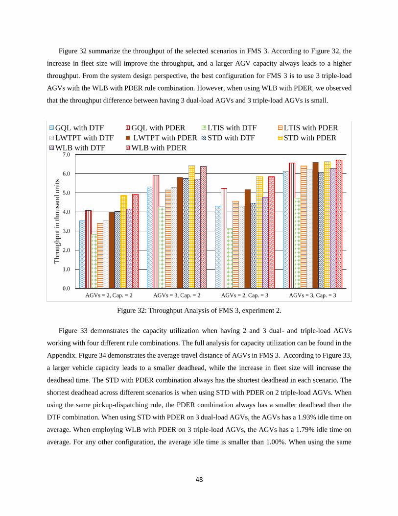
48
Figure 32 summarize the throughput of the selected scenarios in FMS 3. According to Figure 32, the
increase in fleet size will improve the throughput, and a larger AGV capacity always leads to a higher
throughput. From the system design perspective, the best configuration for FMS 3 is to use 3 triple-load
AGVs with the WLB with PDER rule combination. However, when using WLB with PDER, we observed
that the throughput difference between having 3 dual-load AGVs and 3 triple-load AGVs is small.
Figure 32: Throughput Analysis of FMS 3, experiment 2.
Figure 33 demonstrates the capacity utilization when having 2 and 3 dual- and triple-load AGVs
working with four different rule combinations. The full analysis for capacity utilization can be found in the
Appendix. Figure 34 demonstrates the average travel distance of AGVs in FMS 3. According to Figure 33,
a larger vehicle capacity leads to a smaller deadhead, while the increase in fleet size will increase the
deadhead time. The STD with PDER combination always has the shortest deadhead in each scenario. The
shortest deadhead across different scenarios is when using STD with PDER on 2 triple-load AGVs. When
using the same pickup-dispatching rule, the PDER combination always has a smaller deadhead than the
DTF combination. When using STD with PDER on 3 dual-load AGVs, the AGVs has a 1.93% idle time on
average. When employing WLB with PDER on 3 triple-load AGVs, the AGVs has a 1.79% idle time on
average. For any other configuration, the average idle time is smaller than 1.00%. When using the same
0.0
1.0
2.0
3.0
4.0
5.0
6.0
7.0
AGVs = 2, Cap. = 2 AGVs = 3, Cap. = 2 AGVs = 2, Cap. = 3 AGVs = 3, Cap. = 3
Thro
ughput
in t
housa
nd u
nit
s
GQL with DTF GQL with PDER LTIS with DTF LTIS with PDER
LWTPT with DTF LWTPT with PDER STD with DTF STD with PDER
WLB with DTF WLB with PDER
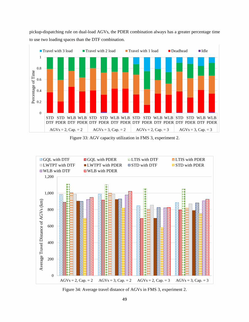
49
pickup-dispatching rule on dual-load AGVs, the PDER combination always has a greater percentage time
to use two loading spaces than the DTF combination.
Figure 33: AGV capacity utilization in FMS 3, experiment 2.
Figure 34: Average travel distance of AGVs in FMS 3, experiment 2.
0
0.2
0.4
0.6
0.8
1
STD
DTF
STD
PDER
WLB
DTF
WLB
PDER
STD
DTF
STD
PDER
WLB
DTF
WLB
PDER
STD
DTF
STD
PDER
WLB
DTF
WLB
PDER
STD
DTF
STD
PDER
WLB
DTF
WLB
PDER
AGVs = 2, Cap. = 2 AGVs = 3, Cap. = 2 AGVs = 2, Cap. = 3 AGVs = 3, Cap. = 3
Per
cen
tag
e o
f T
ime
Travel with 3 load Travel with 2 load Travel with 1 load Deadhead Idle
0
200
400
600
800
1,000
1,200
AGVs = 2, Cap. = 2 AGVs = 3, Cap. = 2 AGVs = 2, Cap. = 3 AGVs = 3, Cap. = 3
Aver
age
Tra
vel
Dis
tan
ce o
f A
GV
s (k
m)
GQL with DTF GQL with PDER LTIS with DTF LTIS with PDER
LWTPT with DTF LWTPT with PDER STD with DTF STD with PDER
WLB with DTF WLB with PDER
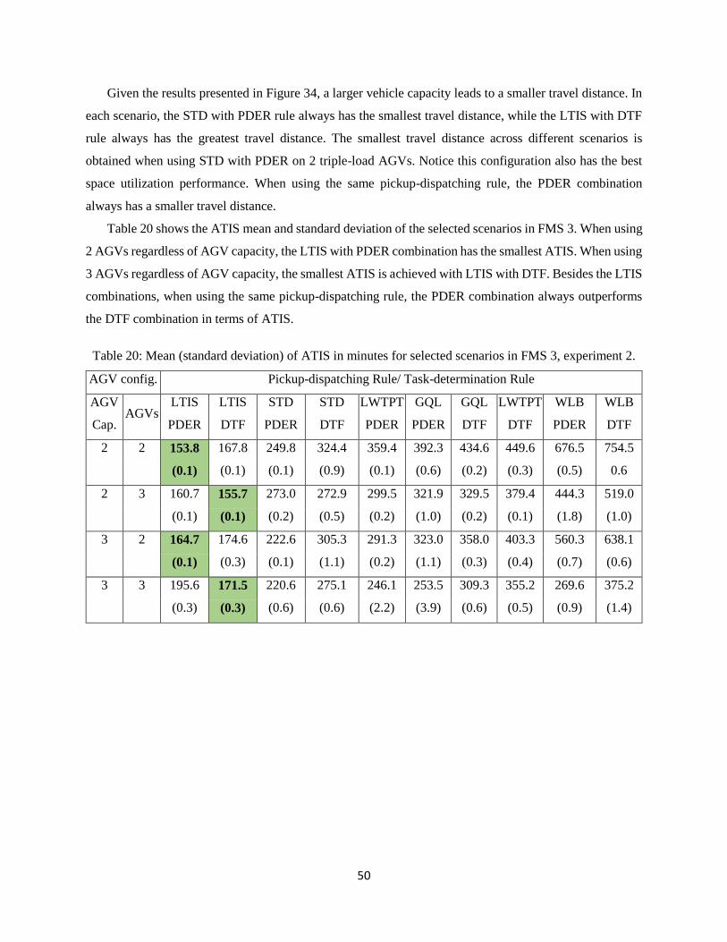
50
Given the results presented in Figure 34, a larger vehicle capacity leads to a smaller travel distance. In
each scenario, the STD with PDER rule always has the smallest travel distance, while the LTIS with DTF
rule always has the greatest travel distance. The smallest travel distance across different scenarios is
obtained when using STD with PDER on 2 triple-load AGVs. Notice this configuration also has the best
space utilization performance. When using the same pickup-dispatching rule, the PDER combination
always has a smaller travel distance.
Table 20 shows the ATIS mean and standard deviation of the selected scenarios in FMS 3. When using
2 AGVs regardless of AGV capacity, the LTIS with PDER combination has the smallest ATIS. When using
3 AGVs regardless of AGV capacity, the smallest ATIS is achieved with LTIS with DTF. Besides the LTIS
combinations, when using the same pickup-dispatching rule, the PDER combination always outperforms
the DTF combination in terms of ATIS.
Table 20: Mean (standard deviation) of ATIS in minutes for selected scenarios in FMS 3, experiment 2.
AGV config. Pickup-dispatching Rule/ Task-determination Rule
AGV
Cap. AGVs
LTIS
PDER
LTIS
DTF
STD
PDER
STD
DTF
LWTPT
PDER
GQL
PDER
GQL
DTF
LWTPT
DTF
WLB
PDER
WLB
DTF
2 2 153.8 167.8 249.8 324.4 359.4 392.3 434.6 449.6 676.5 754.5
(0.1) (0.1) (0.1) (0.9) (0.1) (0.6) (0.2) (0.3) (0.5) 0.6
2 3 160.7 155.7 273.0 272.9 299.5 321.9 329.5 379.4 444.3 519.0
(0.1) (0.1) (0.2) (0.5) (0.2) (1.0) (0.2) (0.1) (1.8) (1.0)
3 2 164.7 174.6 222.6 305.3 291.3 323.0 358.0 403.3 560.3 638.1
(0.1) (0.3) (0.1) (1.1) (0.2) (1.1) (0.3) (0.4) (0.7) (0.6)
3 3 195.6 171.5 220.6 275.1 246.1 253.5 309.3 355.2 269.6 375.2
(0.3) (0.3) (0.6) (0.6) (2.2) (3.9) (0.6) (0.5) (0.9) (1.4)
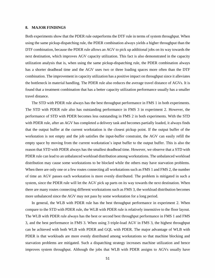
51
8. MAJOR FINDINGS
Both experiments show that the PDER rule outperforms the DTF rule in terms of system throughput. When
using the same pickup-dispatching rule, the PDER combination always yields a higher throughput than the
DTF combination, because the PDER rule allows an AGV to pick up additional jobs on its way towards the
next destination, which improves AGV capacity utilization. This fact is also demonstrated in the capacity
utilization analysis that is, when using the same pickup-dispatching rule, the PDER combination always
has a shorter deadhead time and the AGV uses two or three loading spaces more often than the DTF
combination. The improvement in capacity utilization has a positive impact on throughput since it alleviates
the bottleneck in material handling. The PDER rule also reduces the average travel distance of AGVs. It is
found that a treatment combination that has a better capacity utilization performance usually has a smaller
travel distance.
The STD with PDER rule always has the best throughput performance in FMS 1 in both experiments.
The STD with PDER rule also has outstanding performance in FMS 3 in experiment 2. However, the
performance of STD with PDER becomes less outstanding in FMS 2 in both experiments. With the STD
with PDER rule, after an AGV has completed a delivery task and becomes partially loaded, it always finds
that the output buffer at the current workstation is the closest pickup point. If the output buffer of the
workstation is not empty and the job satisfies the input-buffer constraint, the AGV can easily refill the
empty space by moving from the current workstation’s input buffer to the output buffer. This is also the
reason that STD with PDER always has the smallest deadhead time. However, we observe that a STD with
PDER rule can lead to an unbalanced workload distribution among workstations. The unbalanced workload
distribution may cause some workstations to be blocked while the others may have starvation problems.
When there are only one or a few routes connecting all workstations such as FMS 1 and FMS 2, the number
of time an AGV passes each workstation is more evenly distributed. The problem is mitigated in such a
system, since the PDER rule will let the AGV pick up parts on its way towards the next destination. When
there are many routes connecting different workstations such as FMS 3, the workload distribution becomes
more unbalanced since the AGV may not pass by some workstation for a long period.
In general, the WLB with PDER rule has the best throughput performance in experiment 2. When
compare to the STD with PDER rule, the WLB with PDER rule is relatively insensitive to the floor layout.
The WLB with PDER rule always has the best or second best throughput performance in FMS 1 and FMS
3, and the best performance in FMS 3. When using 3 triple-load AGV in FMS 3, the highest throughput
can be achieved with both WLB with PDER and GQL with PDER. The major advantage of WLB with
PDER is that workloads are more evenly distributed among workstations so that machine blocking and
starvation problems are mitigated. Such a dispatching strategy increases machine utilization and hence
improves system throughput. Although the jobs that WLB with PDER assigns to AGVs usually have
52
stronger impact on maximizing throughput, there is a tradeoff between delivering more parts and delivering
more urgent parts. As FMS 1 has a loop floor layout, it is more important to have AGVs pick up and deliver
parts more frequently than finding the urgent jobs. When there are many routes connecting different
workstations such as FMS 3, it is more important to have a balanced system.
Both experiments show that the PDER rule also has outstanding performances in terms of the average
time parts spend in the system. When using the same pickup dispatching rule, the PDER rule outperforms
the DTF rule except for the LTIS case. In the first experiment, the STD with PDER rule has the best ATIS
performance. However, in experiment 2, the smallest average time in system is always achieved with either
a LTIS with PDER or LTIS with DTF rule. When using 3 dual-load AGVs in FMS 1, there is no significant
difference between LTIS with PDER and LTIS with DTF in terms of ATIS. When using two triple-load
AGVs in FMS 3, the LTIS with PDER, LTIS with DTF, and STD with PDER all have the best ATIS
performance. The essential goal of the LTIS rule is to minimize the time in system of parts. A part waiting
at the pickup point of the Entry station always has a smaller time in system than those parts in the output
buffers of workstations. Thus, the AGVs will drive the manufacturing system to focus on completing the
parts that already left the Entry station. This effect ensures the minimizing time in system but reduces the
number of parts pulled into the system, thus limiting throughput. In contrast, we observe the downside of
the WLB rule (regardless of the task-determination rule) is the large ATIS. In order to avoid machine
starvation problems upstream, the WLB rule tends to pull more parts into the system than other pickup-
dispatching rules.
When the system is not over capacitated, the increase in fleet size always has a positive impact on
system throughput and ATIS. However, there is a tradeoff between system performance and AGV
performance. As there are more AGVs in the system, the number of jobs distributed to each vehicle becomes
smaller. For example, if two AGVs have the same or similar low-cost pickup points, they have to compete
for the limited number of low-cost jobs. The AGV that loses the bidding may not find another low-cost job
so that the empty loading spaces will not be utilized. Recall that an AGV can accept a job only if the job’s
succeeding input buffer has no more than 6 parts waiting to be processed. These are the reasons that some
systems have larger AGV idle time when using 3 AGVs. When using the STD with PDER rule, the
competition has a large impact on capacity utilization. This is because if the AGV loses in an bidding, it
will has to find another job, which may be further from its current location. It also explains the reason that
a larger fleet size always increase the average travel distance of AGVs when using STD with PDER.
It is found that a larger AGV capacity can improve the system throughput. However, the relationship
between system throughput and cost of material handling system is not always linear. For example, the
STD with PDER rule always yields the highest throughput in FMS 1. When using 2 AGVs, the throughput
of using triple-load AGVs is around 11.9% higher than using dual-load AGVs. When using 3 AGVs, the

53
use of triple-load AGVs only increases the throughput by 3.5%. In this case, the three additional loading
spaces only increase the throughput by around 236 parts. As the throughput of a system is getting closer to
its upper bound, the impacts of increasing fleet size and AGV capacity become smaller.
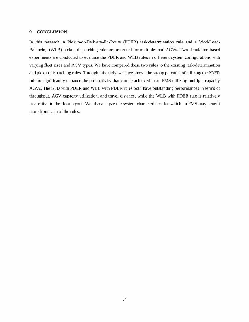
54
9. CONCLUSION
In this research, a Pickup-or-Delivery-En-Route (PDER) task-determination rule and a WorkLoad-
Balancing (WLB) pickup-dispatching rule are presented for multiple-load AGVs. Two simulation-based
experiments are conducted to evaluate the PDER and WLB rules in different system configurations with
varying fleet sizes and AGV types. We have compared these two rules to the existing task-determination
and pickup-dispatching rules. Through this study, we have shown the strong potential of utilizing the PDER
rule to significantly enhance the productivity that can be achieved in an FMS utilizing multiple capacity
AGVs. The STD with PDER and WLB with PDER rules both have outstanding performances in terms of
throughput, AGV capacity utilization, and travel distance, while the WLB with PDER rule is relatively
insensitive to the floor layout. We also analyze the system characteristics for which an FMS may benefit
more from each of the rules.
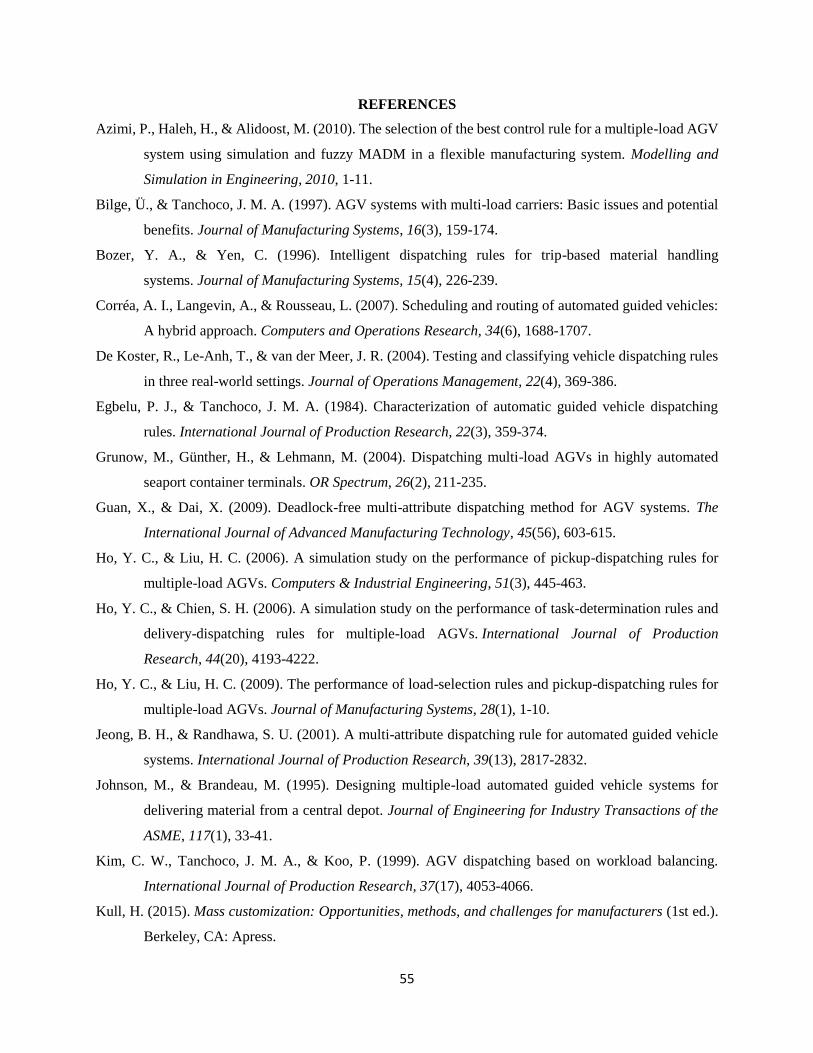
55
REFERENCES
Azimi, P., Haleh, H., & Alidoost, M. (2010). The selection of the best control rule for a multiple-load AGV
system using simulation and fuzzy MADM in a flexible manufacturing system. Modelling and
Simulation in Engineering, 2010, 1-11.
Bilge, Ü., & Tanchoco, J. M. A. (1997). AGV systems with multi-load carriers: Basic issues and potential
benefits. Journal of Manufacturing Systems, 16(3), 159-174.
Bozer, Y. A., & Yen, C. (1996). Intelligent dispatching rules for trip-based material handling
systems. Journal of Manufacturing Systems, 15(4), 226-239.
Corréa, A. I., Langevin, A., & Rousseau, L. (2007). Scheduling and routing of automated guided vehicles:
A hybrid approach. Computers and Operations Research, 34(6), 1688-1707.
De Koster, R., Le-Anh, T., & van der Meer, J. R. (2004). Testing and classifying vehicle dispatching rules
in three real-world settings. Journal of Operations Management, 22(4), 369-386.
Egbelu, P. J., & Tanchoco, J. M. A. (1984). Characterization of automatic guided vehicle dispatching
rules. International Journal of Production Research, 22(3), 359-374.
Grunow, M., Günther, H., & Lehmann, M. (2004). Dispatching multi-load AGVs in highly automated
seaport container terminals. OR Spectrum, 26(2), 211-235.
Guan, X., & Dai, X. (2009). Deadlock-free multi-attribute dispatching method for AGV systems. The
International Journal of Advanced Manufacturing Technology, 45(56), 603-615.
Ho, Y. C., & Liu, H. C. (2006). A simulation study on the performance of pickup-dispatching rules for
multiple-load AGVs. Computers & Industrial Engineering, 51(3), 445-463.
Ho, Y. C., & Chien, S. H. (2006). A simulation study on the performance of task-determination rules and
delivery-dispatching rules for multiple-load AGVs. International Journal of Production
Research, 44(20), 4193-4222.
Ho, Y. C., & Liu, H. C. (2009). The performance of load-selection rules and pickup-dispatching rules for
multiple-load AGVs. Journal of Manufacturing Systems, 28(1), 1-10.
Jeong, B. H., & Randhawa, S. U. (2001). A multi-attribute dispatching rule for automated guided vehicle
systems. International Journal of Production Research, 39(13), 2817-2832.
Johnson, M., & Brandeau, M. (1995). Designing multiple-load automated guided vehicle systems for
delivering material from a central depot. Journal of Engineering for Industry Transactions of the
ASME, 117(1), 33-41.
Kim, C. W., Tanchoco, J. M. A., & Koo, P. (1999). AGV dispatching based on workload balancing.
International Journal of Production Research, 37(17), 4053-4066.
Kull, H. (2015). Mass customization: Opportunities, methods, and challenges for manufacturers (1st ed.).
Berkeley, CA: Apress.
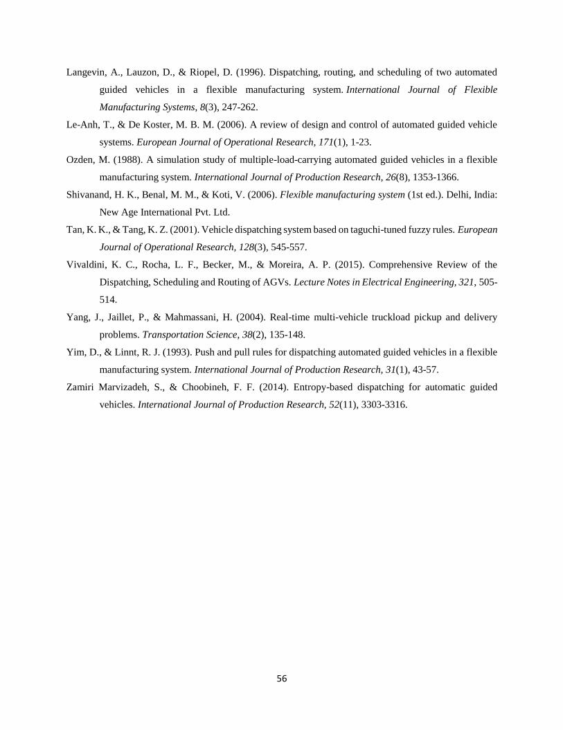
56
Langevin, A., Lauzon, D., & Riopel, D. (1996). Dispatching, routing, and scheduling of two automated
guided vehicles in a flexible manufacturing system. International Journal of Flexible
Manufacturing Systems, 8(3), 247-262.
Le-Anh, T., & De Koster, M. B. M. (2006). A review of design and control of automated guided vehicle
systems. European Journal of Operational Research, 171(1), 1-23.
Ozden, M. (1988). A simulation study of multiple-load-carrying automated guided vehicles in a flexible
manufacturing system. International Journal of Production Research, 26(8), 1353-1366.
Shivanand, H. K., Benal, M. M., & Koti, V. (2006). Flexible manufacturing system (1st ed.). Delhi, India:
New Age International Pvt. Ltd.
Tan, K. K., & Tang, K. Z. (2001). Vehicle dispatching system based on taguchi-tuned fuzzy rules. European
Journal of Operational Research, 128(3), 545-557.
Vivaldini, K. C., Rocha, L. F., Becker, M., & Moreira, A. P. (2015). Comprehensive Review of the
Dispatching, Scheduling and Routing of AGVs. Lecture Notes in Electrical Engineering, 321, 505-
514.
Yang, J., Jaillet, P., & Mahmassani, H. (2004). Real-time multi-vehicle truckload pickup and delivery
problems. Transportation Science, 38(2), 135-148.
Yim, D., & Linnt, R. J. (1993). Push and pull rules for dispatching automated guided vehicles in a flexible
manufacturing system. International Journal of Production Research, 31(1), 43-57.
Zamiri Marvizadeh, S., & Choobineh, F. F. (2014). Entropy-based dispatching for automatic guided
vehicles. International Journal of Production Research, 52(11), 3303-3316.

57
APPENDIX
Simio Processes
Figure 35: This is an add-on process for the Source. If there are less than 6 parts in the output buffer of the
Source, the NeedsMore step returns true and a new part will be created. Otherwise, the source will stop
creating new parts.
Figure 36: This is the process invoked by the FindClosestPoint in Figure 13. The IsPickupNodeCloser step
returns true if the AGV does not have an available delivery point or the closest pickup point is closer to the
AGV’s current location when compare to the closest delivery point. If the statement is false, the
NextDropOff step will set the next destination to be the closest delivery point.
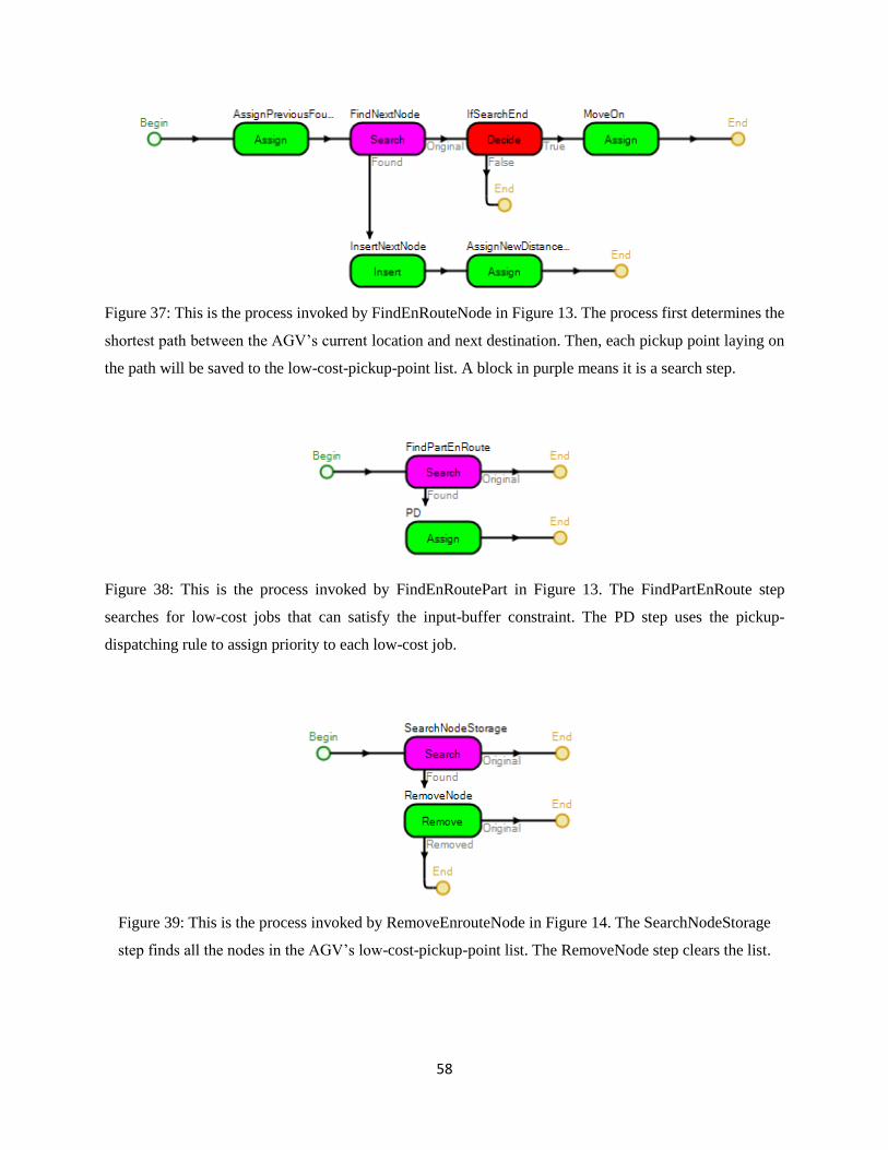
58
Figure 37: This is the process invoked by FindEnRouteNode in Figure 13. The process first determines the
shortest path between the AGV’s current location and next destination. Then, each pickup point laying on
the path will be saved to the low-cost-pickup-point list. A block in purple means it is a search step.
Figure 38: This is the process invoked by FindEnRoutePart in Figure 13. The FindPartEnRoute step
searches for low-cost jobs that can satisfy the input-buffer constraint. The PD step uses the pickup-
dispatching rule to assign priority to each low-cost job.
Figure 39: This is the process invoked by RemoveEnrouteNode in Figure 14. The SearchNodeStorage
step finds all the nodes in the AGV’s low-cost-pickup-point list. The RemoveNode step clears the list.
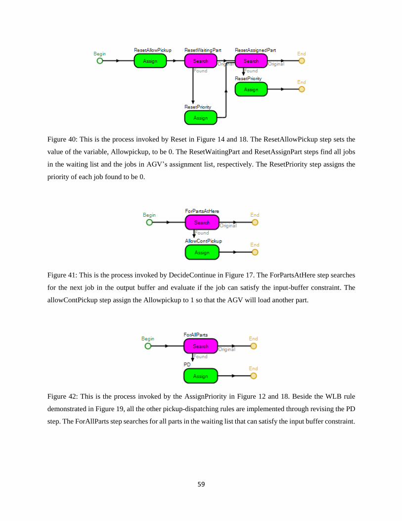
59
Figure 40: This is the process invoked by Reset in Figure 14 and 18. The ResetAllowPickup step sets the
value of the variable, Allowpickup, to be 0. The ResetWaitingPart and ResetAssignPart steps find all jobs
in the waiting list and the jobs in AGV’s assignment list, respectively. The ResetPriority step assigns the
priority of each job found to be 0.
Figure 41: This is the process invoked by DecideContinue in Figure 17. The ForPartsAtHere step searches
for the next job in the output buffer and evaluate if the job can satisfy the input-buffer constraint. The
allowContPickup step assign the Allowpickup to 1 so that the AGV will load another part.
Figure 42: This is the process invoked by the AssignPriority in Figure 12 and 18. Beside the WLB rule
demonstrated in Figure 19, all the other pickup-dispatching rules are implemented through revising the PD
step. The ForAllParts step searches for all parts in the waiting list that can satisfy the input buffer constraint.
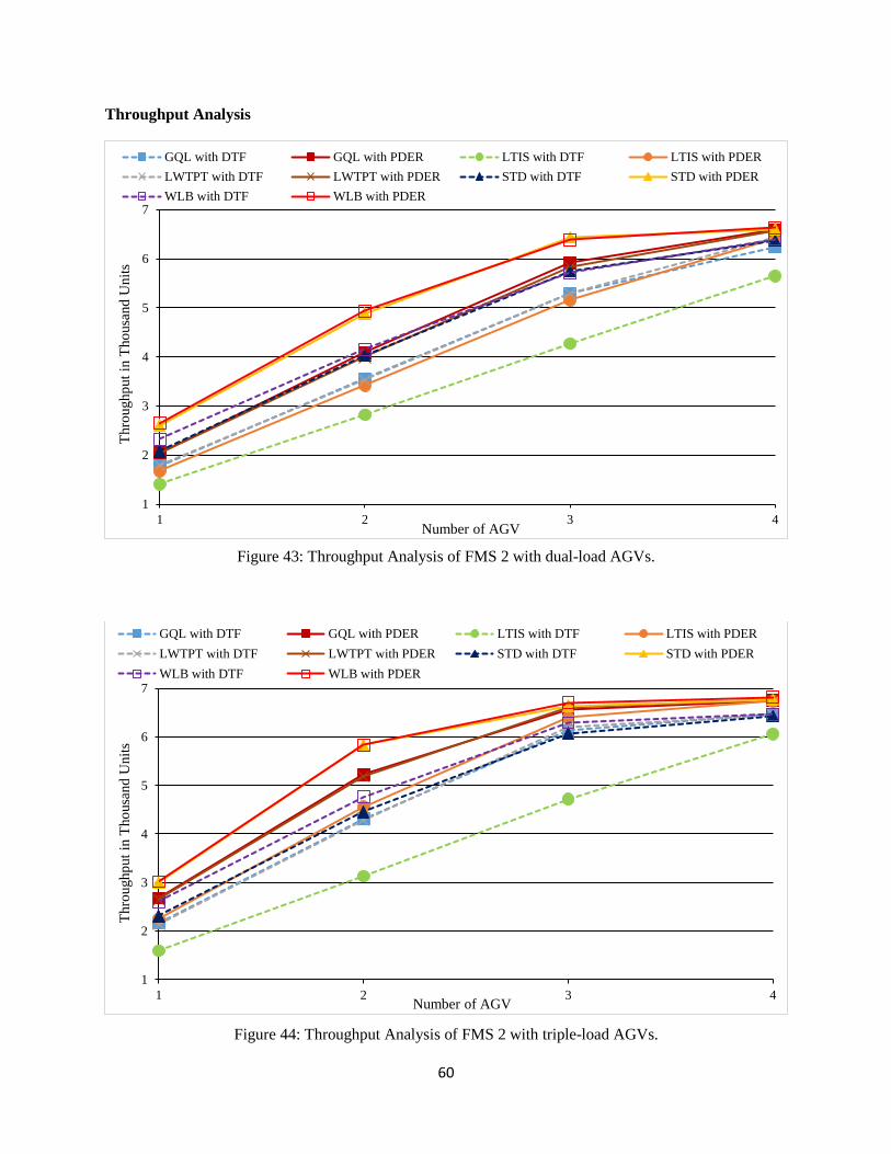
60
Throughput Analysis
Figure 43: Throughput Analysis of FMS 2 with dual-load AGVs.
Figure 44: Throughput Analysis of FMS 2 with triple-load AGVs.
1
2
3
4
5
6
7
1 2 3 4
Thro
ughp
ut
in T
ho
usa
nd
Unit
s
Number of AGV
GQL with DTF GQL with PDER LTIS with DTF LTIS with PDER
LWTPT with DTF LWTPT with PDER STD with DTF STD with PDER
WLB with DTF WLB with PDER
1
2
3
4
5
6
7
1 2 3 4
Thro
ughp
ut
in T
ho
usa
nd
Unit
s
Number of AGV
GQL with DTF GQL with PDER LTIS with DTF LTIS with PDER
LWTPT with DTF LWTPT with PDER STD with DTF STD with PDER
WLB with DTF WLB with PDER
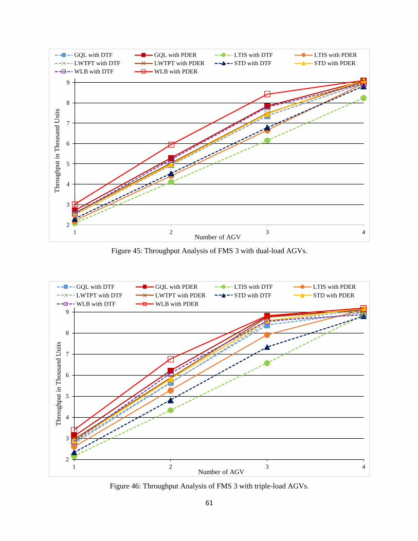
61
Figure 45: Throughput Analysis of FMS 3 with dual-load AGVs.
Figure 46: Throughput Analysis of FMS 3 with triple-load AGVs.
2
3
4
5
6
7
8
9
1 2 3 4
Thro
ughp
ut
in T
ho
usa
nd
Unit
s
Number of AGV
GQL with DTF GQL with PDER LTIS with DTF LTIS with PDER
LWTPT with DTF LWTPT with PDER STD with DTF STD with PDER
WLB with DTF WLB with PDER
2
3
4
5
6
7
8
9
1 2 3 4
Thro
ughp
ut
in T
ho
usa
nd
Unit
s
Number of AGV
GQL with DTF GQL with PDER LTIS with DTF LTIS with PDER
LWTPT with DTF LWTPT with PDER STD with DTF STD with PDER
WLB with DTF WLB with PDER
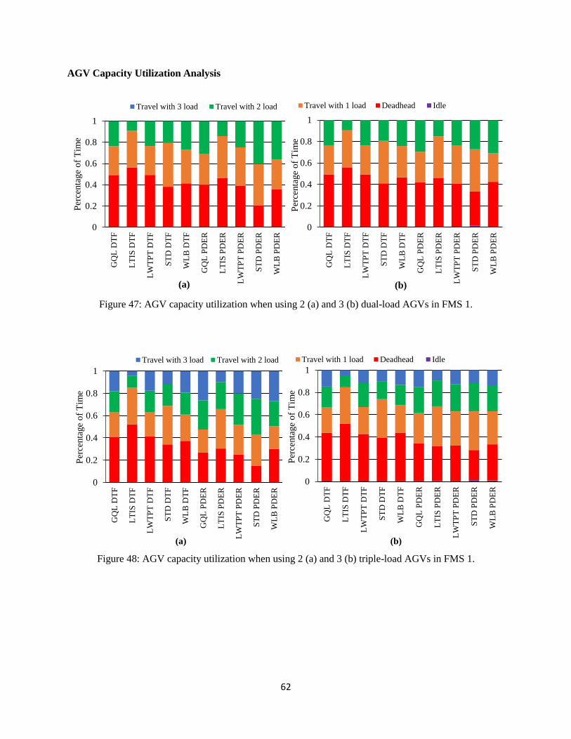
62
AGV Capacity Utilization Analysis
Figure 47: AGV capacity utilization when using 2 (a) and 3 (b) dual-load AGVs in FMS 1.
Figure 48: AGV capacity utilization when using 2 (a) and 3 (b) triple-load AGVs in FMS 1.
0
0.2
0.4
0.6
0.8
1G
QL
DT
F
LT
IS D
TF
LW
TP
T D
TF
ST
D D
TF
WL
B D
TF
GQ
L P
DE
R
LT
IS P
DE
R
LW
TP
T P
DE
R
ST
D P
DE
R
WL
B P
DE
R
Per
centa
ge
of
Tim
e
(a)
Travel with 3 load Travel with 2 load
0
0.2
0.4
0.6
0.8
1
GQ
L D
TF
LT
IS D
TF
LW
TP
T D
TF
ST
D D
TF
WL
B D
TF
GQ
L P
DE
R
LT
IS P
DE
R
LW
TP
T P
DE
R
ST
D P
DE
R
WL
B P
DE
R
Per
centa
ge
of
Tim
e(b)
Travel with 1 load Deadhead Idle
0
0.2
0.4
0.6
0.8
1
GQ
L D
TF
LT
IS D
TF
LW
TP
T D
TF
ST
D D
TF
WL
B D
TF
GQ
L P
DE
R
LT
IS P
DE
R
LW
TP
T P
DE
R
ST
D P
DE
R
WL
B P
DE
R
Per
centa
ge
of
Tim
e
(a)
Travel with 3 load Travel with 2 load
0
0.2
0.4
0.6
0.8
1
GQ
L D
TF
LT
IS D
TF
LW
TP
T D
TF
ST
D D
TF
WL
B D
TF
GQ
L P
DE
R
LT
IS P
DE
R
LW
TP
T P
DE
R
ST
D P
DE
R
WL
B P
DE
R
Per
centa
ge
of
Tim
e
(b)
Travel with 1 load Deadhead Idle
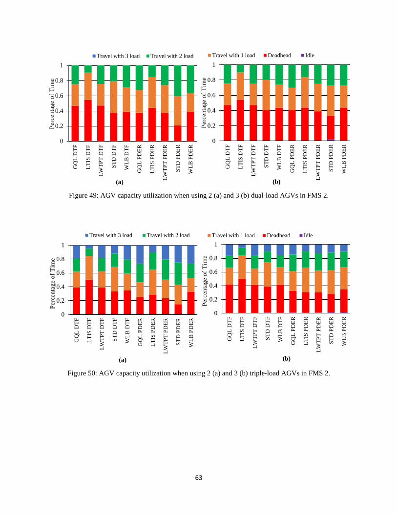
63
Figure 49: AGV capacity utilization when using 2 (a) and 3 (b) dual-load AGVs in FMS 2.
Figure 50: AGV capacity utilization when using 2 (a) and 3 (b) triple-load AGVs in FMS 2.
0
0.2
0.4
0.6
0.8
1
GQ
L D
TF
LT
IS D
TF
LW
TP
T D
TF
ST
D D
TF
WL
B D
TF
GQ
L P
DE
R
LT
IS P
DE
R
LW
TP
T P
DE
R
ST
D P
DE
R
WL
B P
DE
R
Per
centa
ge
of
Tim
e
(a)
Travel with 3 load Travel with 2 load
0
0.2
0.4
0.6
0.8
1
GQ
L D
TF
LT
IS D
TF
LW
TP
T D
TF
ST
D D
TF
WL
B D
TF
GQ
L P
DE
R
LT
IS P
DE
R
LW
TP
T P
DE
R
ST
D P
DE
R
WL
B P
DE
R
Per
centa
ge
of
Tim
e
(b)
Travel with 1 load Deadhead Idle
0
0.2
0.4
0.6
0.8
1
GQ
L D
TF
LT
IS D
TF
LW
TP
T D
TF
ST
D D
TF
WL
B D
TF
GQ
L P
DE
R
LT
IS P
DE
R
LW
TP
T P
DE
R
ST
D P
DE
R
WL
B P
DE
R
Per
centa
ge
of
Tim
e
(a)
Travel with 3 load Travel with 2 load
0
0.2
0.4
0.6
0.8
1
GQ
L D
TF
LT
IS D
TF
LW
TP
T D
TF
ST
D D
TF
WL
B D
TF
GQ
L P
DE
R
LT
IS P
DE
R
LW
TP
T P
DE
R
ST
D P
DE
R
WL
B P
DE
R
Per
centa
ge
of
Tim
e
(b)
Travel with 1 load Deadhead Idle
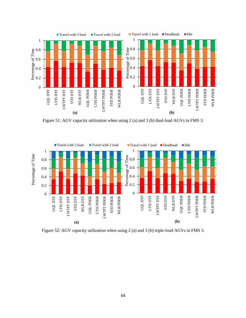
64
Figure 51: AGV capacity utilization when using 2 (a) and 3 (b) dual-load AGVs in FMS 3.
Figure 52: AGV capacity utilization when using 2 (a) and 3 (b) triple-load AGVs in FMS 3.
0
0.2
0.4
0.6
0.8
1
GQ
L D
TF
LT
IS D
TF
LW
TP
T D
TF
ST
D D
TF
WL
B D
TF
GQ
L P
DE
R
LT
IS P
DE
R
LW
TP
T P
DE
R
ST
D P
DE
R
WL
B P
DE
R
Per
centa
ge
of
Tim
e
(a)
Travel with 3 load Travel with 2 load
0
0.2
0.4
0.6
0.8
1
GQ
L D
TF
LT
IS D
TF
LW
TP
T D
TF
ST
D D
TF
WL
B D
TF
GQ
L P
DE
R
LT
IS P
DE
R
LW
TP
T P
DE
R
ST
D P
DE
R
WL
B P
DE
R
Per
centa
ge
of
Tim
e
(b)
Travel with 1 load Deadhead Idle
0
0.2
0.4
0.6
0.8
1
GQ
L D
TF
LT
IS D
TF
LW
TP
T D
TF
ST
D D
TF
WL
B D
TF
GQ
L P
DE
R
LT
IS P
DE
R
LW
TP
T P
DE
R
ST
D P
DE
R
WL
B P
DE
R
Per
centa
ge
of
Tim
e
(a)
Travel with 3 load Travel with 2 load
0
0.2
0.4
0.6
0.8
1
GQ
L D
TF
LT
IS D
TF
LW
TP
T D
TF
ST
D D
TF
WL
B D
TF
GQ
L P
DE
R
LT
IS P
DE
R
LW
TP
T P
DE
R
ST
D P
DE
R
WL
B P
DE
R
Per
centa
ge
of
Tim
e
(b)
Travel with 1 load Deadhead Idle