1

Design and Analysis of Joint Data Detection

and Frequency/Phase Estimation AlgorithmsChun-Hao Hsu Student Member, IEEE,

and Achilleas Anastasopoulos, Member, IEEE

Submitted: April 15, 2004; Revised December 5, 2004

Abstract

The problem of joint data detection and frequency/phase estimation is considered in this work. The

traditional belief regarding exact generalized-likelihood-based joint detection and estimation is that its

complexity is exponential in the sequence length N . This belief is justified due to the memory imposed

on the transmitted sequence by the lack of knowledge of the auxiliary channel parameters. In this paper,

we show that the exact solution can be performed with O(N4) worst-case complexity regardless of the

operating signal-to-noise ratio. The concepts used in the proof of the polynomial complexity result are

also utilized to evaluate tight performance bounds on the exact and a family of approximate algorithms.

I. INTRODUCTION

Coherent data communication requires perfect knowledge of the frequency and phase of

the carrier signal. In practical communication systems, however, the mobility of the transmit-

ter/receiver, in conjunction with the ambient and electronic noise at the receiver circuitry results

in a time-varying phase that is unknown to the receiver. The presence of this frequency/phase

jitter has multiple effects on the transmitted signal, the most severe of which is distortion of the

transmitted signal and generation of inter-symbol interference (ISI) which becomes significant

This work was supported in part by the National Science Foundation under Grant CCF-0346977.

This paper was presented in part at the International Conference on Communications (ICC), Paris, France, June 2004.

The authors are with Electrical Engineering and Computer Science Department, University of Michigan, Ann Arbor, MI

48109-2122, (e-mail: chhsu@umich.edu; anastas@umich.edu).

2

as the frequency/phase dynamics increase. Nevertheless, even when the channel dynamics are

slow, the effect is a multiplicative phase distortion that can cause a significant performance loss,

if not accounted for at the receiver.

There are three basic techniques (see [1] for a tutorial review) for detecting data in the presence

of frequency/phase jitter: (i) a training sequence is transmitted periodically that aids at frequency

and phase estimation, followed by coherent data detection; (ii) the received signal is passed

through a memoryless nonlinearity (e.g., squaring binary phase shift keying (BPSK) signals,)

that eliminates the data dependence, thus allowing channel estimation, followed by coherent

data detection; and (iii) joint data detection and frequency/phase estimation. Clearly, the first

two schemes do not exploit all the channel information available at the received sequence. As

a result, the first two solutions are adequate for high signal-to-noise ratios (SNRs) and slow

channel dynamics, but they perform very poorly (in terms of bandwidth efficiency or bit-error-

rate (BER)) in more severe scenarios. Thus, when high-performance codes are employed over

fast channels, some sort of joint detection and estimation needs to be performed.

Motivated by the desire to exploit the information from the whole sequence while keeping a

low computational complexity, several joint detection/estimation algorithms have been proposed

in the literature. These can be classified into the following two categories. The first category

involves alternate maximization (or more formally, expectation maximization (EM)), where

the tasks of channel-conditioned data detection and data-conditioned channel estimation are

performed iteratively starting from an initial channel estimate, until convergence occurs [2]–[4].

The second category of algorithms is based on a suboptimal search over the set of all sequences

by appropriately pruning the sequence tree according to a tree-pruning algorithm, such as the

T-algorithm [5], the M-algorithm [6], or the per-survivor processing (PSP) algorithm [7]–[11].

It is noted that the above mentioned approaches are valid for any joint data detection and

channel estimation problem and not only for the particular problem of joint data detection and

frequency/phase estimation discussed in this paper. The impetus for the aforementioned research

on approximate algorithms was the belief that the exact solution of the joint data detection and

3

parameter estimation problem has exponential complexity with respect to the sequence length.

Since future communication systems will operate close to their theoretical limits, joint data

detection and parameter estimation will become indispensable in achieving the highest possible

performance with the given resources, and thus, the following questions arise: (i) how accurate is

the conventional wisdom that exact joint data detection and frequency/phase estimation requires

exponential complexity with respect to the sequence length? (ii) what is the impact of a negative

answer to the above question on the design of approximate algorithms? (iii) how can the

complexity/performance tradeoff of these approximate algorithms be analyzed, and how can

it be improved?

In this paper we continue the work initiated in [12] in trying to provide answers to the

above questions. In particular, it is shown here that exact, generalized-likelihood-based, joint

detection and frequency/phase jitter estimation of uncoded sequences is a polynomial-complexity

problem in the sequence length. Furthermore, the proposed technique can be generalized to solve

the problem of symbol-by-symbol soft-decision generation implied by the min-sum algorithm,

which can be used when turbo-like coded sequences are utilized. In this paper, we concentrate

in the uncoded sequence detection problem, since the extension to symbol-by-symbol soft-

decision generation can be performed in a way similar to the one described in [12]. Furthermore,

based on the proposed exact solution, we develop a class of approximate algorithms. Finally, a

framework for analyzing the performance of both exact and approximate algorithms at arbitrary

SNR is proposed. In the case of performance analysis for the exact algorithms, it is shown

that analysis is possible exactly due to the novel polynomial-complexity structure. For the

approximate algorithms, it is shown that their performance can get close to that of the exact

algorithms with reasonable complexity.

The remaining of the paper is structured as follows. Section II develops the system and channel

model under consideration. The polynomial-complexity exact algorithm for joint data detection

and frequency/phase estimation is developed in Section III, after reviewing the corresponding

results from [12]. Section IV presents the performance analysis for the exact, as well as several

4

approximate techniques. Numerical results are presented in Section V, while the conclusions

are summarized in Section VI. For the sake of clarity, most of the proofs are relegated to an

appendix at the end of the paper.

II. CHANNEL MODEL

Consider the transmission of a length-N sequence of symbols sk ∈ A, where A is a set of

complex-valued numbers with unit magnitude. The equivalent lowpass transmitted signal is of

the form

s(t) =N∑

k=1

sk

√Ekp(t − kT ) (1)

where p(t) is a pulse shape function satisfying the no-ISI Nyquist criterion [13, Section 9.2.1],

with unit energy, T is the symbol duration, and Ek = Es or Ep depending on whether sk is an

information symbol or pilot symbol, respectively. If this signal is transmitted over an additive

white Gaussian noise (AWGN) channel and is further rotated by a phase process φ(t) unknown

to both transmitter and receiver, then the received signal z(t) can be modelled as1

z(t) = s(t)ejφ(t) + n(t) (2)

where n(t) is a zero mean complex white Gaussian process with one-sided power spectral

density level N0. For this observation model, optimal pre-processing depends on the phase

process φ(t) and in the general case should include fractionally-spaced sampling. However, for

the purpose of illustrating the basic ideas, we will assume symbol-spaced sampling, since all

algorithms generalize easily to the fractionally-space model. We will further assume perfect epoch

synchronization. Then, if the phase rotation process φ(t) is modelled by a constant unknown

1In this model, amplitude variations are ignored. This is done mainly in order to isolate the effects of phase rotation on

the system performance. This assumption may be justified for channels where the phase rotation is due to imperfect local

oscillators, and not due to user mobility. In the latter case, this model can be justified by the existence of an automatic gain

control mechanism that compensates for the amplitude variations.

5

phase θ ∈ [0, 2π), i.e., if

φ(t) = θ ∀t ∈ [0, NT ), (3)

then there will be no ISI and we have the following equivalent discrete-time model

z = Dsejθ + n (4)

where s ! [s1, s2, . . . , sN ]T ,D is a diagonal matrix with diagonal elements (√

E1,√

E2, . . . ,√

EN ),

z ! [z1, z2, . . . , zN ]T is the vector of symbol-spaced observations, and n ! [n1, n2, . . . , nN ]T

is a vector of i.i.d. zero-mean circularly symmetric complex Gaussian random variables with

variance N0/2 per real an imaginary component. On the other hand, if the phase rotation process

is modelled by

φ(t) = 2π(fd/T )t + θ ∀t ∈ [0, NT ), (5)

where fd ∈ [0, 1) is the normalized frequency jitter, and θ ∈ [0, 2π) is the phase shift, then as

shown in [1] under the assumption of no ISI and perfect gain control, the discrete-time model

becomes

zk = sk

√Eke

j(2πfdk+θ) + nk ∀k = 1, 2, . . . , N. (6)

III. ALGORITHMS FOR EXACT GENERALIZED-LIKELIHOOD DETECTION

For this section and the rest of the paper, we will restrict our attention to the special case

where we use equally probable antipodal signaling, i.e., A = {+1,−1} for simplicity. Moreover,

we will assume that the first one, and the first two symbols are pilot symbols for models (4),

and (6), respectively. With a little abuse of notation, it is understood that all following detection

algorithms are applied only to information symbols by setting beforehand the pilot symbols to +1.

However, we note that all the algorithms and results presented in this paper can be generalized

to arbitrary alphabet A, unequal a-priori probabilities, arbitrary pilot symbol positioning, and

energy assignments with a complexity increase by a factor O(|A|2).

6

A. Background: The Constant Phase Model

In this subsection, we review the low complexity exact generalized-likelihood algorithm pro-

posed in [12], [14], [15] for completeness and for the purpose of showing the basic idea from

which we develop the exact algorithm for the more complicated model (6). The sequence

estimate based on the generalized-likelihood ratio test (GLRT) for model (4) can be written

in the following double maximization form

sGLRT ! arg maxs∈AN

{max

θ∈[0,2π)p(z|s, θ)

}= arg max

s∈AN

{max

θ∈[0,2π)%{zHDsejθ}

}(7a)

= arg maxs∈AN

|zHDs|. (7b)

It is well known that, under the assumption that the constant phase rotation θ is uniformly

distributed in [0, 2π), the GLRT solution coincides with the maximum likelihood sequence

detection (MLSD) solution. Furthermore, this optimal solution can be obtained exactly with

O(N log N) complexity as follows (for details on the correctness of the algorithm, refer to [12]).

1) Calculate the set of partitioning points (or thresholds) from the received signal z as follows

Φ ! {φi ∈ [0, 2π) : φi ! ∠zi ±π

2, ∀i = 2, 3, . . . , N} (8)

2) Sort Φ so that Φ = {0 ≤ t1 ≤ t2 ≤ . . . ≤ t2(N−1) ≤ 2π}. We use j(i) to denote the index

of the observation symbol zj(i) associated with ti.

3) Find the candidate sequence supported by the first partition, which contains phase 0,

s1 = s(0) (9)

where

s(θ) ! arg maxs∈AN

%{zHDsejθ} (10)

4) Sequentially evaluate the candidate sequence si+1 from si by flipping the j(i)th bit of si.

5) As explicitly proved in [12], sGLRT must be one of the candidate sequences s1, s2, . . . , s2(N−1).

Hence we have

sGLRT = arg maxs∈{s1,s2,...,s2(N−1)}

%{zHDsejθ(s)} = arg maxs∈{s1,s2,...,s2(N−1)}

|zHDs| (11)

7

where

θ(s) ! arg maxθ∈[0,2π)

%{zHDsejθ} = −∠(zHDs) (12)

The actual algorithm in [12], [14], [15] further simplifies the metric evaluation in (11), so

that the overall complexity is determined by the sorting in step 2) which can be performed in

O(N log N) time. Note that the basic idea behind the algorithm is to partition the parameter

space [0, 2π) in such a way that performing coherent sequence detection with one hypothesized

parameter taken from each set of the partition provides a sufficient set of candidate sequences

for the GLRT problem.

B. The Linear Phase Model

Consider the model in (6). The GLRT solution is given by

sGLRT ! arg maxs

{max

(fd,θ)∈Λp(z|s, fd, θ)

}(13)

where Λ ! [0, 1)× [0, 2π) is the 2-dimensional parameter space over which maximization of the

unknown parameters fd and θ is performed for each possible transmitted sequence. In the rest

of the section, we will aim at finding this exact GLRT solution with polynomial complexity.

Defining

fd(s) ! arg maxfd

{max

θp(z|s, fd, θ)

}= arg max

fd

∣∣∣∣∣∑

k

z∗k sk

√Eke

j2πfdk

∣∣∣∣∣ (14a)

and

θ(s) ! arg maxθ

{max

fd

p(z|s, fd, θ)

}= −∠

(∑

k

z∗k sk

√Eke

j2πfd(s)k

)(14b)

to be the sequence-conditioned phase/frequency estimates, we have

sGLRT = arg maxs∈AN

p(z|s, fd(s), θ(s)) (15)

Looking at (15) one can make the following observation. There are two sources of complexity in

finding the GLRT solution. The first one is combinatorial in nature and is related to the exponen-

tial growth of sequences (or metrics) that need to be maximized. The second source of complexity

8

is computational in nature and is related to the evaluation of each metric p(z|s, fd(s), θ(s)) for

a given hypothesized sequence. This latter complexity is linear in N for the constant phase

model as evidenced in (7b). It should be clear however, that there is no hope in finding a

closed-form solution for the metric p(z|s, fd(s), θ(s)), since this is equivalent to finding a closed-

form solution to the sequence-conditioned frequency estimate fd(s) in (14a). But this, in turn,

involves maximization of the magnitude of the discrete-time Fourier transform (DTFT) of the

sequence {zks∗k√

Ek}Nk=1 over the continuous interval [0, 1) [1]. Therefore, frequency estimation

can only be performed within a pre-specified accuracy with finite complexity in all practical

algorithms. Since this complexity is unavoidable even when the data sequence is known, we

are only interested in the first source of complexity manifesting itself through the combinatorial

explosion of the data sequences. As can be seen in (15), even if we omit the frequency-estimation

complexity, the exact GLRT solution still appears to demand O(2N) complexity; we will now

propose an exact algorithm, which performs this task with O(N4) complexity regardless of the

SNR.

Defining a parameter-conditioned sequence estimate

s(fd, θ) ! arg maxs∈AN

p(z|s, fd, θ), (16)

the GLRT problem can be restated as

sGLRT ! max(fd,θ)∈Λ

p(z|s(fd, θ), fd, θ). (17)

Furthermore, collecting all candidate GLRT solutions in the sufficient set

T ! {s(fd, θ)|(fd, θ) ∈ Λ}, (18)

the GLRT problem becomes

sGLRT = arg maxs∈T

p(z|s, fd(s), θ(s)). (19)

It is now clear how one should proceed to prove the polynomial-complexity result: if the size

of T grows only polynomially with N , and T can be constructed by a polynomial-complexity

algorithm, then using (19) one can solve the problem with polynomial combinatorial complexity.

9

As shown in [12] for a general GLRT problem, constructing the sufficient set T is equivalent

to partitioning the parameter space Λ into subsets in such a way that all parameter pairs (fd, θ)

in each subset result in the same sequence s(fd, θ). It was further shown that this partitioning

can be accomplished by superimposing the boundaries defined by equations of the form

|zk −√

Ek(+1)ej(2πfdk+θ)|2 = |zk −√

Ek(−1)ej(2πfdk+θ)|2

⇔ 2πfdk + θ = ∠zk ±π

2+ 2πm, (20)

for all k = 1, 2, . . . , N , and all integers m. An example of the resulting partitioned parameter

space is shown in Fig. 1.

By observing that there are 2k lines for each k, we conclude that there are O(N 2) lines in

total implied by (20). Using a well-known result from computational geometry [16], one can

deduce that at most |T | = O(N4) polygons can be generated by superimposing O(N2) lines

and that there is an O(N4)-complexity algorithm that can construct these polygons, and thus

the sufficient set T . We further improve this estimate by using the additional information that

every line with k = i intersects at most one line with k = j, j )= i, and is parallel to all lines

with k = i. Indeed, due to the above observation, it is straightforward to show that there are at

most |T | = O(N3) partitions resulted from these lines since each line intersects at most N − 1

other lines. Moreover, to compute all intersection points of each additional line at k = i with

all previously drawn lines, the following algorithm can be used.

1) Find the entrance intersection point on the polygon adjacent to the left or upper boundary of

the parameter space Λ. It is sufficient to look only at the left and upper boundary, because

all lines have negative slopes. The complexity of this step is O(i2) for all 2i lines.

2) Find the exit intersection point among all sides of this polygon. Note that the number of

sides per polygon is constant on the average, resulting in constant complexity for this step.

3) Identify the next polygon (constant complexity with proper indexing). If there is no next

polygon, i.e., the exit point hits the lower or right boundary, then quit. Otherwise, go to

step 2.

10

Since there are O(N 2) lines in total, and each line visits at most N polygons as shown above,

we have shown that the size of the partition and its construction complexity is O(N3).

After constructing all O(N3) polygons, we take one parameter pair (fd, θ) from each polygon

and do coherent symbol by symbol detection hypothesizing (fd, θ) as the CSI. The resulting

O(N3) sequences from all polygons then constitute the the sufficient set T . Finally, the frequency

estimate and the noncoherent metric is evaluated for each of these sequences and is maximized

to find the GLRT solution according to

sGLRT = arg maxs∈T

∣∣∣∣∣

N∑

k=1

z∗k sk

√Eke

j2πfd(s)k

∣∣∣∣∣ . (21)

Since these two final steps require O(N) complexity for each polygon and since we have O(N3)

polygons, we have verified that the whole algorithm finds the exact GLRT solution with O(N4)

complexity. We summarize the above discussion in the following proposition.

Proposition 1 The proposed algorithm in this subsection finds the exact GLRT solution with

worst case complexity O(N4) when omitting the complexity of the frequency estimator, where

N is the sequence length.

Proof: Follows from the above discussion and the framework developed in [12].

IV. PERFORMANCE ANALYSIS OF EXACT AND APPROXIMATE ALGORITHMS

The purpose of this section is to demonstrate that the polynomial-complexity results developed

above, aside from their conceptual value, are also useful in at least two additional respects.

The first is that they enable accurate performance analysis of the corresponding exact GLRT

algorithms, which would otherwise be impossible or result in loose performance bounds. The

second is that they imply a family of approximate algorithms that can be easily implemented

and analyzed. In the following, the exact and two approximate algorithms are analyzed for the

constant phase model and one approximate algorithm is analyzed for the linear phase model.

11

A. Constant Phase Model: Exact GLRT Algorithm

In this subsection, we present a performance analysis for the polynomial-complexity exact

GLRT algorithm for the model in (4). The resulting performance upper bound turns out to be

extremely tight as can be seen in section V, and is now given by the following proposition.

Proposition 2 Under the assumptions of the model in (4), the sequence error probability for the

exact GLRT solution (which is the same as the optimal MLSD solution), can be upper bounded

by

PMLSD ≤2N−2∑

w=1

∫ ∞

0

R(r, Et,EtN0

2)Q1(

r|Et − 2wEs|√2wEtEs(Et − wEs)N0

,r√

Et√2wEs(Et − wEs)N0

)dr

+

∫ ∞

0

R(r, Et,EtN0

2)Q1(

r|Ep − (N − 1)Es|√2(N − 1)EtEsEpN0

,r√

Et√2(N − 1)EsEpN0

)dr

+ 1 − (1 − Q(

√2Es

N0))N−1, (22a)

where

Et ! Ep + (N − 1)Es (22b)

denotes the total signalling energy,

R(r, s,σ2) ! r

σ2e−

r2+s2

2σ2 I0(rs

σ2) (22c)

is a Ricean density with I0(·) being the 0th-order modified Bessel function of the first kind, and

Q1(·, ·), Q(·) are the the Marcum’s Q function, and the Gaussian tail function, respectively.

Proof: See Appendix A.

The main idea of the proof is to use union bound over a much smaller sufficient set of

sequences rather than all the 2N sequences. This can be done only because the set of all possible

MLSD solutions had been tremendously reduced to have a size linear in N as was shown in the

previous section.

12

B. Constant Phase Model: Pilot-Only (PO) Algorithm

It is possibly the simplest approximate algorithm, which uses the channel information provided

by the pilot symbol only, and performs symbol-by-symbol detection as follows

si = arg maxs∈A

p(zi|s, z1) i = 2, . . . , N, (23)

This pilot-only (PO) algorithm has complexity O(N), and its performance is given in the

following proposition.

Proposition 3 The probability of bit error of the PO algorithm is exactly

Pb(PO) = 1 −∫ 2π

0

∫ π2

−π2

T (y + x,Es

N0)T (x,

Ep

N0)dydx (24)

where

T (x, S) ! 1

2πe−S +

√S

πcos(x)e−S sin2(x)

(1 − Q(

√2S cos(x))

)(25)

is the probability density function (pdf) of the phase component of the complex Gaussian random

variable with mean√

S and variance 1. Therefore, the corresponding probability of sequence

error is

PPO = 1 −(∫ 2π

0

∫ π2

−π2

T (y + x,Es

N0)T (x,

Ep

N0)dydx

)N−1

(26)

Proof: See Appendix B.

It is worth noting that even if we drop the magnitude information of z1 and condition only on

∠z1 in (23), we obtain the same performance in this uncoded sequence case. However, if we are

also interested in the soft decisions of the receiver as required in the coded sequence case, then

the magnitude information provided by the pilot symbol would help improve the performance

as shown in [17].

13

C. Constant Phase Model: Uniform Sampling (US) Algorithm

Motivated by the exact algorithm described in Section IV-A, we now consider a simple

approximate analogue of it and analyze its performance. The idea behind this algorithm is

that instead of optimally partitioning the parameter space [0, 2π)–a process that has complexity

O(N log N)–one can partition the parameter space in a sensible, but somewhat arbitrary way,

in order to reduce complexity. The simplest such partitioning is the uniform partitioning (or

sampling), which results in the following algorithm.

1) Define L samples {ai}Li=1 as

ai ! 2πi

L, ∀ i = 1, 2, . . . , L (27)

2) Obtain L candidate sequences s(ai) for all i and select

sUS = arg maxs(ai):i∈{1,2,...,L}

|zHDs(ai)| (28)

This algorithm has complexity O(LN) and a characterization of its performance is given by

the following proposition.

Proposition 4 Under the assumption that L ≥ 2, the probability of sequence error for the US

algorithm can be bounded by

PMLSD ≤ PUS ≤PMLSD + (N − 1)(N − 2)

∫ ∞

0

R(r, Et,EtN0

2)

[∫ πL

− πL

T (θ − π

2,

Es

Et(Et − Es)N0r2)dθ

]2

dr (29a)

=PMLSD + O(N2

L2e−

EsN0 ) (29b)

Proof: See Appendix C.

The main idea behind the proof can again be attributed to the parameter space partitioning

perspective. The event that we miss the MLSD solution is exactly the event that none of our

sampling points is in the same partition with the MLSD solution. It is the probability of this

event that is characterized and upper bounded in the proof.

14

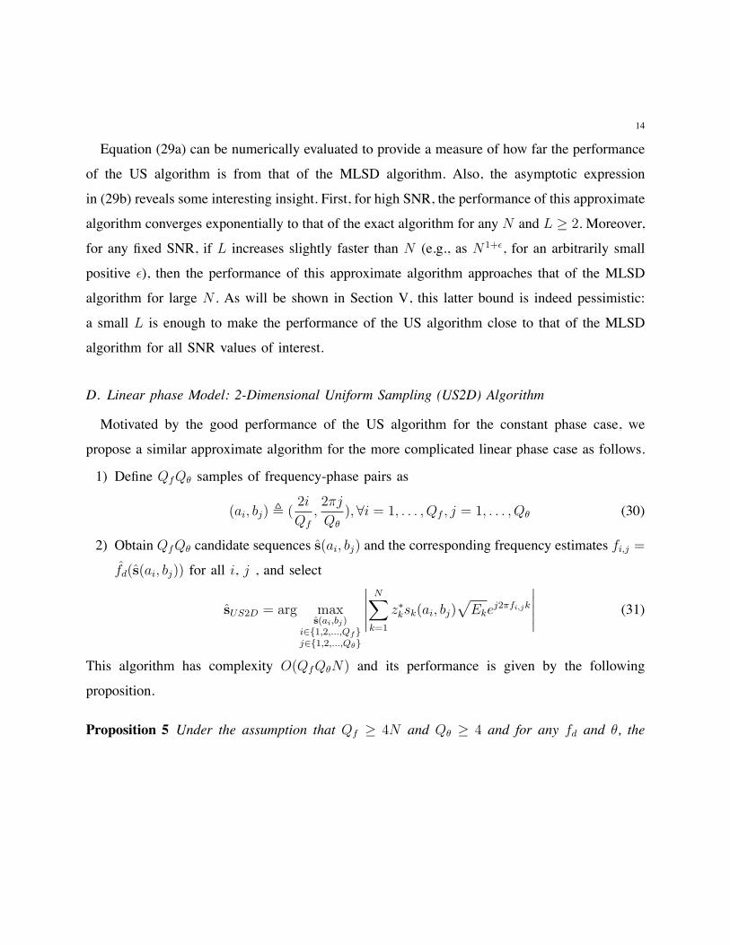
Equation (29a) can be numerically evaluated to provide a measure of how far the performance

of the US algorithm is from that of the MLSD algorithm. Also, the asymptotic expression

in (29b) reveals some interesting insight. First, for high SNR, the performance of this approximate

algorithm converges exponentially to that of the exact algorithm for any N and L ≥ 2. Moreover,

for any fixed SNR, if L increases slightly faster than N (e.g., as N1+ε, for an arbitrarily small

positive ε), then the performance of this approximate algorithm approaches that of the MLSD

algorithm for large N . As will be shown in Section V, this latter bound is indeed pessimistic:

a small L is enough to make the performance of the US algorithm close to that of the MLSD

algorithm for all SNR values of interest.

D. Linear phase Model: 2-Dimensional Uniform Sampling (US2D) Algorithm

Motivated by the good performance of the US algorithm for the constant phase case, we

propose a similar approximate algorithm for the more complicated linear phase case as follows.

1) Define QfQθ samples of frequency-phase pairs as

(ai, bj) ! (2i

Qf,2πj

Qθ),∀i = 1, . . . , Qf , j = 1, . . . , Qθ (30)

2) Obtain QfQθ candidate sequences s(ai, bj) and the corresponding frequency estimates fi,j =

fd(s(ai, bj)) for all i, j , and select

sUS2D = arg maxs(ai,bj)

i∈{1,2,...,Qf}j∈{1,2,...,Qθ}

∣∣∣∣∣

N∑

k=1

z∗ksk(ai, bj)√

Ekej2πfi,jk

∣∣∣∣∣ (31)

This algorithm has complexity O(QfQθN) and its performance is given by the following

proposition.

Proposition 5 Under the assumption that Qf ≥ 4N and Qθ ≥ 4 and for any fd and θ, the

15

probability of sequence error for the US2D algorithm can be bounded by

PCSI ≤ PUS2D ≤PCSI + PGLRT + {1 − 2N∏

k=1

(1 − ql(k)) +N∏

k=1

(1 − 2ql(k))}

+{1 − 2(1 − qu)N + (1 − 2qu)N

}(32a)

=PCSI + PGLRT + O(N2

Qfe−

EsN0 ) + O(

N

Qθe−

EsN0 ) (32b)

where PCSI and PGLRT are the probability of error for the perfect channel state information

(CSI) and the exact GLRT algorithms, respectively, and

ql(k) =

∫ 2πkQf

0

T (x − π

2,Es

N0) + T (x +

π

2,Es

N0)dx (33a)

qu =

∫ 2πQθ

0

T (x − π

2,Es

N0) + T (x +

π

2,Es

N0)dx. (33b)

Proof: See Appendix D.

This result is very similar in spirit to Proposition 4. One difference is that because of the

additional frequency jitter, we may need to increase Qf quadratically with N in order to have a

performance close to that of the exact GLRT algorithm. Another difference is that in this case,

the upper and lower bounds do not agree even for large Qf and Qθ.

V. NUMERICAL RESULTS

In this section numerical results are presented for the exact and approximate algorithms

developed earlier for both the constant and the linear phase models.

A. The Constant Phase Model

Fig. 2 compares the performance bounds for the three algorithms (where the expression for

the PO algorithm is exact) developed in Section IV for model (4) with optimally chosen pilot

energies versus the information bit SNR, Eb/N0def= (Et/N0)/(N − 1)/ log2 |A|. Also shown is

the PCSI performance curve, and a “naive” MLSD bound obtained by a union bound over all

2N sequences. As can be seen in the figure, the upper bound of the US algorithm, which is

16

obtained by substituting the MLSD bound into (29a), performs almost identically to the upper

bound of the exact MLSD algorithm, and is very close to the performance curve of the perfect

CSI receiver. With a moderate choice of L = 8 in the approximate algorithm, it performs equally

well for both N = 4 and N = 32 cases. As compared with the PO algorithm, we gain 2 dB

when N = 4 and about 0.5 dB when N = 32 by using the US algorithm. Note also that the

upper bound for the MLSD algorithm is actually very tight since the CSI performance is a lower

bound.

B. The Linear Phase Model

In this subsection we provide various simulation results regarding the implementation of the

US2D algorithm. For simplicity, we use Ep = Es instead of optimizing over Ep throughout our

simulations.

One way to perform frequency estimation for a given sequence, is to zero-pad the sequence

with D zeros and perform an (N + D)-point FFT to find the frequency component with the

maximum magnitude. This entails O((N +D) log(N +D)) complexity per sequence, which can

be undesirable in the US2D algorithm. Since the US2D algorithm is aiming at low complexity, we

adopt the simplest version of the Luise and Reggiannini (L&R) estimator [18] for this algorithm,

which evaluates a frequency estimate as

fd(s) = ∠N−1∑

i=1

(zi+1s∗i+1)(zis

∗i )

∗, (34)

thus having linear complexity in N . Note that in general, the L&R estimator can use more

autocorrelation coefficients than just the first one as in this case. As can be seen in Fig. 3, the

considerably much faster L&R estimator suffers only about 1 dB performance loss (at BER=10−3)

compared to the higher accuracy FFT estimators. Therefore, in all the following simulations, we

will employ this L&R frequency estimator for the US2D algorithm.

To examine the effect of Qθ in the US2D algorithm, we have nullified the effect of Qf by

using a large Qf such that no performance can be gained by further increasing this Qf . Fig. 4

17

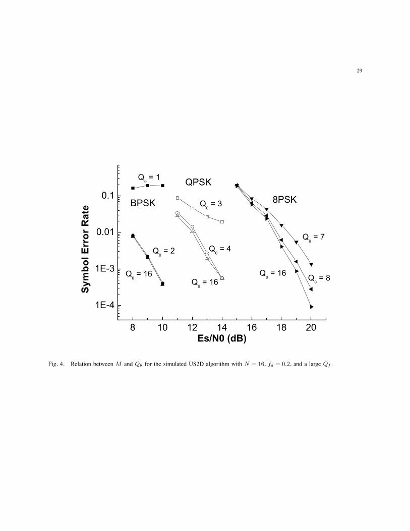
shows the performances of the US2D algorithm for a large enough Qf , different values of Qθ,

and different M-PSK alphabets. As can be seen in the figure, very little improvement can be

gained by selecting Qθ > M regardless of N (Similar simulations for N = 32 were performed,

resulting in the same conclusion). This suggests that Proposition 5, which shows that performance

behaves as O( NQθ

), provides a conservative estimate.

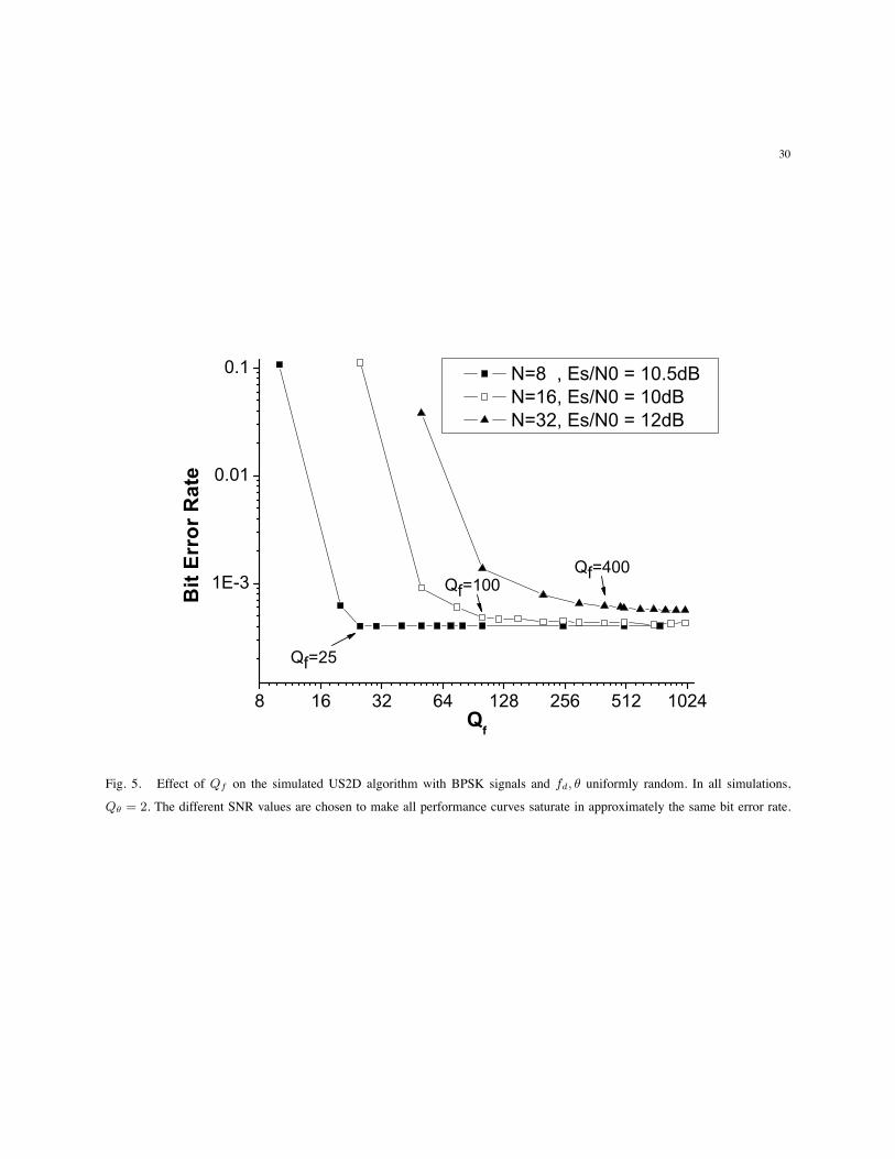
Due to the above observation, we fix Qθ = M in the US2D algorithm and investigate how Qf

affects performance. Fig. 5 clearly shows that to achieve the best performance, Qf should grow

approximately quadratically with N as predicted in Proposition 5. This result for Qf together

with the previous one for Qθ suggests that it is possible to employ an O(N3) complexity US2D

algorithm to achieve a near-exact performance.

Fig. 6 shows that the US2D algorithm with a fast L&R frequency estimator can indeed achieve

a performance close to that of the exact GLRT algorithm, which employs a very accurate FFT-

based frequency estimator, by choosing a moderate Qf and Qθ. Notice that the number of

frequency samples was increased quadratically with N . Also shown is the performance of an

ad-hoc pilot-only algorithm, which first estimates fd and θ using the first two pilots and then does

symbol-by-symbol detection assuming the estimated CSI. It is obvious that for this linear phase

model, it is much more desirable to extract the channel information from the whole received

sequence by performing joint detection/estimation schemes rather than restricting our attention

only to the channel information provided by pilots. Also shown in Fig. 6 are the upper bounds

derived in Proposition 5. However, the parameters used for obtaining these bounds were Qθ = 8

and Qf = 8N which are different from those used to obtain the simulated performance. This was

due to the fact that the bound is valid for Qθ ≥ 4 and Qf ≥ 4N as mentioned in Proposition 5.

VI. CONCLUSION AND DISCUSSION

Several low complexity joint detection/estimation algorithms for noncoherent channels with

an unknown phase rotation are presented and analyzed in this paper. If the phase process is

modelled by a constant phase shift, then we showed that the low complexity US algorithm can

be applied, which yields a performance close to that of the ML decoder with perfect CSI. In the

18

case that the phase process is modelled by both a frequency jitter and a phase shift, we showed

that the exact GLRT solution can be obtained with combinatorial complexity O(N4) or well

approximated by the proposed US2D algorithm with complexity O(QfQθN).

When powerful codes are utilized, symbol by symbol soft decisions will be desired by the

decoder for iterative decoding. The proposed algorithms can also be adapted to provide this

information. It is very similar to the one discussed in [12], and the additional manipulation will

only increase the whole complexity of the algorithms by a factor of N .

We conclude by noting that the basic idea behind the exact algorithms is to think of decision

regions in the parameter space rather than in the observation space as is the traditional approach.

This is helpful since in the discussed problems, the dimension of the observation space grows

with N , while that of the parameter space remains fixed. It is thus expected that similar results

will hold every time the number of independent parameters that need to be estimated grows

slower than N .

APPENDIX

A. Proof of Proposition 2

Let s0, sCSI be the transmitted sequence and the detected sequence for the hypothetical receiver

that has perfect CSI. We have

PMLSD = Pr(sMLSD )= s0) = Pr(sMLSD )= s0, sCSI = s0) + Pr(sMLSD )= s0, sCSI )= s0)

≤Pr({sMLSD )= s0} ∩ {s0 = sj for some 1 ≤ j ≤ 2(N − 1)}) + Pr(sCSI )= s0)

≤Pr

⋃

1≤i≤2(N−1),i&=j

{|zHDs0| < |zHDsi|}

+ 1 − (1 − Q(

√2Es

N0))N−1 (35)

where si,∀i )= 0 are the candidate sequences as defined in the exact GLRT algorithm. To further

evaluate the first term of (35), we define X ! zHDs0 and Yi ! zHDsi for 1 ≤ i ≤ 2(N − 1).

Since X and Y ′i s are jointly Gaussian, we have

p(Yi|X) = CN (Yi,Et − 2wiEs

EtX,

4wiEs(Et − wiEs)N0

Et) (36)

19

where CN (·,m,σ2) is the pdf of a complex Gaussian random variable with mean m and variance

σ2, and wi is the number of places where s0 and si differ. Therefore, we have

Pr(∣∣zHDs0

∣∣ <∣∣zHDsi

∣∣) =

∫

CPr(|Yi| > |x||X = x)fX(x)dx (37)

=

∫

C

∫ ∞

|x|R(r,

∣∣∣∣Et − 2wiEs

Et

∣∣∣∣ |x|,2wiEs(Et − wiEs)N0

Et)fX(x)drdx

=

∫ ∞

0

R(r, Et,EtN0

2)Q1(

r|Et − 2wiEs|√2wiEtEs(Et − wiEs)N0

,r√

Et√2wiEs(Et − wiEs)N0

)dr (38)

where C is the set of all complex numbers and fX is the pdf of X . Hence by taking the union

bound in (35) and use the fact that candidate sequences corresponding to neighboring partitions

of [0, 2π) differ in only one symbol, which follows from the structure of the exact polynomial-

complexity algorithm, we obtain (22a).

B. Proof of Proposition 3

Letting z =√

Es+n where n ∼ CN (0, N0), r = |z| and t = ∠z−∠z1, its bit error probability

can be evaluated as follows:

Pb(PO) =Pr

(∫ 2π

0

e2"{z

√Ese−jθ}N0 e

2|z1|√

Ep cos(∠z1−θ)

N0 dθ <

∫ 2π

0

e−2"{z

√Ese−jθ}

N0 e2|z1|

√Ep cos(∠z1−θ)

N0 dθ

)

=Pr

(∫ 2π

0

[e

2r√

Es cos(θ−∠z)N0 − e

−2r√

Es cos(θ−∠z)N0

]e

2|z1|√

Ep cos(∠z1−θ)

N0 dθ < 0

)

=Pr

(∫ 2π

0

sinh(2r√

Es cos(θ − t)

N0)e

2|z1|√

Ep cos(∠z1−θ)

N0 dθ < 0

)(39)

Since sinh(2r√

Es cos(θ)N0

) and e2|z1|

√Ep cos(∠z1−θ)

N0 are both symmetric bell shaped functions of θ in

one period [−π,π], their circular convolution would still be a bell shaped function. Observing

further that∫ 2π

0 sinh(2r√

Es cos(θ−t)N0

)e2|z1|

√Ep cos(∠z1−θ)

N0 dθ attains maximum at t = 0, minimum at

20

t = π and 0 at t = ±π2 , we have

Pb(PO) =1 − p(t ∈ [−π

2,π

2])

=1 − Eθ

[∫ 2π

0

p(∠z ∈ [−π

2+ ∠z1,

π

2+ ∠z1]|θ)f(∠z1|θ)d∠z1

]

=1 − Eθ

[∫ 2π

0

∫ π2 +x

−π2 +x

T (y − θ,Es

N0)dyT (x − θ,

Ep

N0)dx

]

=1 − Eθ

[∫ 2π

0

∫ π2

−π2

T (y + x,Es

N0)T (x,

Ep

N0)dydx

]

=1 −∫ 2π

0

∫ π2

−π2

T (y + x,Es

N0)T (x,

Ep

N0)dydx (40)

It then follows that PPO = 1 − (1 − Pb(PO))N−1.

C. Proof of Proposition 4

The lower bound follows easily by the optimality of the MLSD metric. The upper bound of

PUS is derived as follows:

PUS =Pr(sUS )= s0) = Pr(sUS )= s0, sMLSD = s0) + Pr(sUS )= s0, sMLSD )= s0)

≤Pr(sUS )= sMLSD = s0) + PMLSD (41)

where s0 is the transmitted sequence. The first term of this upper bound can be further bounded

as

Pr(sUS )= sMLSD = s0) ≤ Pr({No sample point is in the same partition with θ(s0)})

=L∑

i=1

Pr(⋃

k,l:k &=l

{φk,φl ∈ (ai, ai+1)} ∩ {θ(s0) ∈ (φk,φl)})

≤L∑

i=1

∑

k,l:k &=l

Eθ

[Pr({φk,φl ∈ [ai, ai+1]} ∩ {θ(s0) ∈ (φk,φl)}|θ)

](42)

21

where the notation φl ∈ [a, b] is used to denote the event that one of the threshold pairs

obtained from zl as in (8) is inside [a, b]. Define

x1 !Epejθ +√

Epn1 (43)

xi !Esejθ + s0,ini ∀i = 2, 3, . . . , N (44)

X !N∑

i=1

xi (45)

We have

φi =∠zi ±π

2= s0,i∠zi ±

π

2= ∠xi ±

π

2∀i = 2, 3, . . . , N (46)

θ(s0) = − ∠(zHs0) = ∠N∑

i=1

(s20,ie

jθ + s0,ini

)= ∠X (47)

Hence

p({φk,φl ∈ [ai, ai+1]} ∩ {θ(s0) is between φk,φl}|θ)

=2

∫

X:∠X∈[ai,ai+1]

∫

xk:∠xk±π2 ∈[ai,∠X]

∫

xl:∠xl±π2 ∈[∠X,ai+1]

f(xk, xl, X|θ)dxldxkdX (48)

which is under the assumption that L ≥ 2 so that the ith pair of thresholds can not lie in the

same sampling interval for all i. Since xi’s are i.i.d. complex Gaussian random variables and X

is the sum of them, we have

f(X|θ) =|X|

πEtN0e−

||X|ej∠X−Etejθ |2EtN0 (49)

f(xl|X, θ) =CN(

xl,Es

EtX,EsN0(1 − Es

Et)

)(50)

f(xk|xl, X, θ) =CN(

xk,Es

Ep + (N − 2)Es(X − xl), EsN0(1 − Es

Ep + (N − 2)Es)

)(51)

Letting

EN−i ![ EsEp+(N−i)Es

]2

Es(1 − EsEp+(N−i)Es

)for i integer (52)

22

to simplify notation, the above integral becomes

2

∫ ∞

0

∫ ai+1

ai

[∫

xl:∠xl±π2 ∈[∠X,ai+1]

∫

θk±π2 ∈[ai,∠X]

T (θk − ∠(X − xl),EN−2

N0|X|2)

|xl|πEsN0(1 − Es

Et)e−

||xl|ej∠xl−Es

EtX|2

EsN0(1−EsEt

) dθkdxl

|X|πEtN0

e−||X|ej∠X−Etejθ |2

EtN0 d∠Xd|X| (53)

Now, observe that the integrand of (53) depends only on θ, which is uniformly distributed in

[0, 2π). Since all sampling intervals have the same lengths, (53) should not depend on the choice

the sampling interval i. Also, note that (53) does not depend on k nor l. Hence, after combining

all the terms, we obtain

Pr(sUS )= sMLSD = s0) ≤ L(N − 1)(N − 2)

∫ ∞

0

∫ 2πL

0

1

2π

[∫ ∠X

−∠X

T (θ1 −π

2,EN−2

N0|X|2)dθ1

]

[∫ 2πL −∠X

− 2πL +∠X

T (θ2 −π

2,EN−1

N0|X|2)dθ2

]R(|X|, Et,

EtN0

2)d∠Xd|X|,

which reduces to (29a).

D. Proof of Proposition 5

The lower bound is obvious. The upper bound can be derived as follows.

PUS2D =Pr(sUS2D )= s0)

=Pr(sUS2D )= s0, sCSI = s0, sGLRT = s0) + Pr(sUS2D )= s0, sCSI )= s0, sGLRT = s0)

+ Pr(sUS2D )= s0, sGLRT )= s0)

≤Pr(sUS2D )= sGLRT = sCSI) + PCSI + PGLRT (54)

The first term of this upper bound can be further calculated as follows

Pr(sUS2D )= sGLRT = sCSI)

≤Pr({no sample pair is in the same partition with(fd, θ)})

=Pr({∃ partitioning lines between (fd, θ) and the nearest four sample pairs}) (55)

23

To evaluate this expression, we define A, B, C and D to be the events that no partitioning line lies

between (fd− 1Qf

, θ) and (fd, θ), (fd, θ)and (fd, θ+ 2πQθ

), (fd, θ)and (fd + 1Qf

, θ), and (fd, θ− 2πQθ

)

and (fd, θ), respectively. Also, recall that all partitioning lines have negative slopes as in (20).

We have

Pr({∃ partitioning lines between (fd, θ) and the nearest four partitioning points})

≤Pr((Ac ∪ Bc) ∩ (Bc ∪ Cc) ∩ (Cc ∪ Dc) ∩ (Dc ∪ Ac)) ≤ Pr(Ac ∩ Cc) + Pr(Bc ∩ Dc). (56)

We define further the event

Ek(f1, θ1, f2, θ2) ! {∃ partitioning lines of the kth symbol that lie between (f1, θ1) and (f2, θ2)}

(57)

and subsequently

ql(k) ! Pr(Ek(fd −1

Qf, θ, fd, θ)|fd, θ) (58a)

qu(k) ! Pr(Ek(fd, θ, fd, θ +2π

Qθ)|fd, θ) (58b)

qr(k) ! Pr(Ek(fd, θ, fd +1

Qf, θ)|fd, θ) (58c)

qd(k) ! Pr(Ek(fd, θ −2π

Qθ, fd, θ)|fd, θ) (58d)

Since conditioning on fd and θ the N sets of partitioning lines are linearly independent, we have

Pr(Ac ∩ Cc) + Pr(Bc ∩ Dc)

=[1 − Pr(A) − Pr(C) + Pr(A ∩ C)] + [1 − Pr(B) − Pr(D) + Pr(B ∩ D)]

=Efd,θ

[{1 −

N∏

k=1

(1 − ql(k)) −N∏

k=1

(1 − qr(k)) +N∏

k=1

(1 − ql(k) − qr(k))

}+

+

{1 −

N∏

k=1

(1 − qu(k)) −N∏

k=1

(1 − qd(k)) +N∏

k=1

(1 − qu(k) − qd(k))

}], (59)

24

where we have used the fact that Qθ ≥ 4 and Qf ≥ 4N in the last equality. Now, since Qf ≥ 4N ,

ql(k) and qr(k) can be evaluated as follows

ql(k) =Pr(1

2πk(∠zk − θ ± π

2) ∈ [fd −

1

Qf, fd]|fd, θ) =

∫ 2πkQf

0

T (x − π

2,Es

N0) + T (x +

π

2,Es

N0)dx

=qr(k) = O(k

Qfe−

EsN0 ) (60)

Similarly, since Qθ ≥ 4, we can evaluate qu(k) and qd(k) as follows

qu(k) =Pr((∠zk − 2πkfd ±π

2) ∈ [θ, θ +

2π

Qθ]|fd, θ) =

∫ 0

− 2πQθ

T (x − π

2,Es

N0) + T (x +

π

2,Es

N0)dx

=qd(k) = O(1

Qθe−

EsN0 ) (61)

Note that ql(k), qr(k), qu(k) and qd(k) actually do not depend on fd and θ, and qu(k) and qd(k)

do not depend on k. Consequently, we have

Pr(sUS2D )= sGLRT = sCSI)

≤{1 − 2N∏

k=1

(1 − ql(k)) +N∏

k=1

(1 − 2ql(k))} +{1 − 2(1 − qu)N + (1 − 2qu)N

}, (62)

which reduces to the expression in (32a).

REFERENCES

[1] M. Morelli and U. Mengali, “Feedforward frequency estimation for PSK: a tutorial review,” European Trans. Telecommun.,

vol. 9, no. 2, pp. 103–116, March/April 1998.

[2] C. N. Georghiades and D. L. Snyder, “The expectation-maximization algorithm for symbol unsynchronized sequence

detection,” IEEE Trans. Communications, vol. 39, no. 1, pp. 54–61, Jan. 1991.

[3] M. Ghosh and C. L. Weber, “Maximum-likelihood blind equalization,” in Proc. SPIE, July 1991, pp. 181–195.

[4] C. N. Georghiades and J. C. Han, “Sequence estimation in the presence of random parameters via the EM algorithm,”

IEEE Trans. Communications, vol. 45, no. 3, pp. 300–308, Mar. 1997.

[5] S. Simmons, “Breadth-first trellis decoding with adaptive effort,” IEEE Trans. Communications, vol. 38, no. 1, pp. 3–12,

Jan. 1990.

[6] J. B. Anderson and S. Mohan, “Sequential coding algorithms: A survey cost analysis,” IEEE Trans. Communications,

vol. 32, pp. 169–176, Feb. 1984.

25

[7] J. Lodge and M. Moher, “Maximum likelihood estimation of CPM signals transmitted over Rayleigh flat fading channels,”

IEEE Trans. Communications, vol. 38, pp. 787–794, June 1990.

[8] R. A. Iltis, “A Bayesian maximum-likelihood sequence estimation algorithm for a priori unknown channels and symbol

timing,” IEEE J. Select. Areas Commun., vol. 10, pp. 579–588, Apr. 1992.

[9] A. N. D’Andrea, U. Mengali, and G. M. Vitetta, “Approximate ML decoding of coded PSK with no explicit carrier phase

reference,” IEEE Trans. Communications, vol. 42, pp. 1033–1040, Feb./Mar./April 1994.

[10] X. Yu and S. Pasupathy, “Innovations-based MLSE for Rayleigh fading channels,” IEEE Trans. Communications, vol. 43,

no. 2/3/4, pp. 1534–1544, Feb./Mar./Apr. 1995.

[11] R. Raheli, A. Polydoros, and C. Tzou, “Per-survivor processing: A general approach to MLSE in uncertain environments,”

IEEE Trans. Communications, vol. 43, no. 2/3/4, pp. 354–364, Feb/Mar/Apr. 1995.

[12] I. Motedayen and A. Anastasopoulos, “Polynomial-complexity noncoherent symbol-by-symbol detection with application

to adaptive iterative decoding of turbo-like codes,” IEEE Trans. Communications, vol. 51, no. 2, pp. 197–207, Feb. 2003.

[13] J. G. Proakis, Digital Communications, 4th ed. New York: McGraw-Hill, 2001.

[14] K. M. Mackenthun, Jr., “A fast algorithm for multiple-symbol differential detection of MPSK,” IEEE Trans. Communica-

tions, vol. 42, pp. 1471–1474, Feb./Mar./Apr. 1994.

[15] W. Sweldens, “Fast block noncoherent decoding,” IEEE Commun. Lett., vol. 5, no. 4, pp. 132–134, Apr. 2001.

[16] H. Edelsbrunner, J. O’Rourke, and R. Seidel, “Constructing arrangements of lines and hyperplanes with applications,”

Society for Industrial and Applied Mathematics Journal on Computing, vol. 15, pp. 341–363, 1986.

[17] R. Nuriyev and A. Anastasopoulos, “Pilot-symbol-assisted coded transmission over the block-noncoherent AWGN channel,”

IEEE Trans. Communications, vol. 51, no. 6, pp. 953–963, June 2003.

[18] M. Luise and R. Reggiannini, “Carrier frequency recovery in all-digital modems for burst-mode transmissions,” IEEE

Trans. Communications, vol. 43, no. 2/3/4, pp. 1169–1178, Mar. 1995.

26

Frequency

Phase

0 1 0

Fig. 1. An example of the partitioned parameter space for N = 4

27

Fig. 2. Analytical results of exact and approximate algorithms for the constant phase model. Above is for N = 4 and below

is for N = 32.

28

Fig. 3. Comparison of simulation results between different frequency estimators for QPSK modulated sequences with N = 16,

fd = 0.2, for the US2D algorithm with large Qf and Qθ = 4.

29

Fig. 4. Relation between M and Qθ for the simulated US2D algorithm with N = 16, fd = 0.2, and a large Qf .

30

Fig. 5. Effect of Qf on the simulated US2D algorithm with BPSK signals and fd, θ uniformly random. In all simulations,

Qθ = 2. The different SNR values are chosen to make all performance curves saturate in approximately the same bit error rate.

31

Fig. 6. Simulation results of the exact GLRT, US2D, and an ad hoc pilot-only algorithm for BPSK modulated sequences with

fd, θ uniformly random. Qθ = 2 and Qf = 10, 40 for N = 5, 10, respectively for the simulated US2D algorithm.