Embed Size (px)
Citation preview
Department of Science and Technology Institutionen för teknik och naturvetenskap Linköping University Linköpings Universitet SE-601 74 Norrköping, Sweden 601 74 Norrköping
Examensarbete LITH-ITN-ED-EX--02/24--SE
Design and Analysis of an All-
optical Free-space Communication link
Fredrik Levander och Per Sakari
020426
LITH-ITN-ED-EX--02/24--SE
Design and Analysis of an All-optical Free-space
communication Link
Examensarbete utfört i teknik vid Linköpings Tekniska Högskola, Campus Norrköping
Fredrik Levander och Per Sakari
Handledare: Thomas Kallstenius och Fredrik Kullander Examinator: Amir Baranzahi
Norrköping den 26 april 2002
Rapporttyp Report category Licentiatavhandling X Examensarbete C-uppsats D-uppsats Övrig rapport _ ________________
Språk Language Svenska/Swedish X Engelska/English _ ________________
Titel Title Design and Analysis of an All-optical Free-space Communication Link Författare Author Fredrik Levander och Per Sakari
Sammanfattning Abstract Free Space Optics (FSO) has received a great deal of attention lately both in the military and civilian information society due to its potentially high capacity, rapid deployment, portability and high security from deception and jamming. The main issue is that severe weather can have a detrimental impact on the performance, which may result in an inadequate availability. This report contains a feasibility study for an all-optical free-space link intended for short-range communication (200-500 m). Laboratory tests have been performed to evaluate the link design. Field tests were made to investigate availability and error performance under the influence of different weather conditions. Atmospheric impact due to turbulence related effects have been studied in detail. The most crucial part of the link design turned out to be the receiver optics and several design solutions were investigated. The main advantage of an all-optical design, compared to commercially available electro-optical FSO-systems, is the potentially lower cost.
ISBN _____________________________________________________ ISRN LITH-ITN-ED-EX--02/24--SE _________________________________________________________________ Serietitel och serienummer ISSN Title of series, numbering ___________________________________
Nyckelord Keyword Master Thesis, Free Space Optics, All-optical, Atmospheric attenuation, Turbulence influence, Availability
Datum Date 2002-04-26
URL för elektronisk version
Avdelning, Institution Division, Department Institutionen för teknik och naturvetenskap Department of Science and Technology
- i -
Abstract Free Space Optics (FSO) has received a great deal of attention lately both in the military and civilian information society due to its potentially high capacity, rapid deployment, portability and high security from deception and jamming. The main issue is that severe weather can have a detrimental impact on the performance, which may result in an inadequate availability. This report contains a feasibility study for an all-optical free-space link intended for short-range communication (200-500 m). Laboratory tests have been performed to evaluate the link design. Field tests were made to investigate availability and error performance under the influence of different weather conditions. Atmospheric impact due to turbulence related effects have been studied in detail. The most crucial part of the link design turned out to be the receiver optics and several design solutions were investigated. The main advantage of an all-optical design, compared to commercially available electro-optical FSO-systems, is the potentially lower cost.
- ii -
Preface and acknowledgements This report concludes our master thesis work founded by Ericsson Research, Ericsson AB (EAB), Kista, and the Swedish Defence Research Agency (FOI), Linköping. It is the final part of our Master degree in Electronics Design Engineering at the University of Linköping, Campus Norrköping. The work has been supervised in collaboration between FOI and ERA and undertaken at FOI. During our thesis work, we have received support from a number of people and we would especially like to thank: First and foremost, our supervisors Thomas Kallstenius at EAB and Fredrik Kullander at FOI for tremendous support and assistance. Göran Bolander, Lars Sjöqvist and other members of the staff at the Department of laser systems at FOI for all knowledge regarding atmospheric influence, optical solutions and laser systems in general. Our reference group at ERA for guidance during the work. Our examiner Amir Baranzahi at ITN, Linköping University. Kerstin Sonesson at Linköpings University for the access to an office during our field tests. Linköping 2002-05-08 Fredrik Levander and Per Sakari
- iii -
Table of contents 1 INTRODUCTION..................................................................................................... 5
1.1 FREE SPACE OPTICS ............................................................................................. 5 1.1.1 Background ................................................................................................. 5 1.1.2 Applications................................................................................................. 5 1.1.3 Advantages and disadvantages ................................................................... 7
1.2 THE THESIS ASSIGNMENT ..................................................................................... 9 1.2.1 The assignment background and motivation............................................... 9 1.2.2 Assignment tasks ....................................................................................... 11
1.3 THE DISPOSITION OF THE THESIS WORK .............................................................. 11 1.4 THE DISPOSITION OF THE REPORT ....................................................................... 11
2 THEORY AND SIMULATIONS .......................................................................... 12 2.1 FUNDAMENTAL OPTICS AND FIBER OPTICS ......................................................... 12
2.1.1 Diffraction ................................................................................................. 12 2.1.2 Chromatic Aberration ............................................................................... 12 2.1.3 Spherical Aberration ................................................................................. 12 2.1.4 Numerical aperture and f-number of lenses.............................................. 13 2.1.5 Numerical aperture of optical fibers......................................................... 14 2.1.6 Graded-Index Multimode Fiber ................................................................ 15 2.1.7 Single-Mode Fiber..................................................................................... 16 2.1.8 Beam width definition................................................................................ 17 2.1.9 Spot size..................................................................................................... 17 2.1.10 Fresnel reflection ...................................................................................... 18 2.1.11 Antireflection coatings .............................................................................. 19
2.2 INVESTIGATED OPTICS........................................................................................ 19 2.2.1 Transmitter optics ..................................................................................... 19 2.2.2 Receiver optics .......................................................................................... 21 2.2.3 Field-of-view, calculations........................................................................ 26 2.2.4 System alignment....................................................................................... 31
2.3 LINK BUDGET ..................................................................................................... 32 2.3.1 Budget overview ........................................................................................ 32 2.3.2 Optical losses ............................................................................................ 33 2.3.3 Ray losses .................................................................................................. 34 2.3.4 Ray losses including errors of a misdirected transmitter ......................... 35 2.3.5 Atmospheric attenuation ........................................................................... 37 2.3.6 Atmospheric turbulence............................................................................. 43 2.3.7 Fiber attenuation....................................................................................... 47 2.3.8 Optical input and output power ................................................................ 48 2.3.9 Conclusion of the link budget.................................................................... 48
3 EXPERIMENTAL .................................................................................................. 50 3.1 LABORATORY TEST – DISTANCE 2 M.................................................................. 50
3.1.2 Result – Coupling efficiency...................................................................... 52 3.2 LABORATORY TEST – DISTANCE 180 M.............................................................. 53
- iv -
3.2.1 Result – Intensity distribution ................................................................... 56 3.2.2 Result – Coupling efficiency...................................................................... 56 3.2.3 Result – Field-of-view ............................................................................... 59
3.3 FIELD TESTS – DISTANCE 420 M......................................................................... 61 3.3.1 Result – Field-of-view ............................................................................... 63 3.3.2 Result – Power fluctuations due to turbulence.......................................... 63 3.3.3 Result – Weather influence........................................................................ 64
3.4 TRANSMISSION USING MMF .............................................................................. 68 3.4.1 Results ....................................................................................................... 70
3.5 BIT-ERROR-RATE TEST – 420 AND 140 M ........................................................... 73 3.5.1 Results ....................................................................................................... 76
4 CONCLUSION........................................................................................................ 81
5 REFERENCES........................................................................................................ 84
6 APPENDIX .............................................................................................................. 86 6.1 ATMOSPHERIC INFLUENCE THEORY.................................................................... 86
6.1.1 Atmospheric attenuation ........................................................................... 86 6.1.2 Atmosphere turbulence.............................................................................. 87
INTRODUCTION
- 5 -
1 Introduction
1.1 Free Space Optics
1.1.1 Background Free Space Optics (FSO) refers to the transmission of modulated visible or infrared (IR) beams through the atmosphere to obtain broadband communications. FSO systems can function over distances of several kilometers. Communication is theoretically possible as long as the line of sight between the transmitter and the receiver is clear, and as long as the transmitted power is high enough to overcome atmospheric attenuation. Like in fiber optics, lasers are used to transmit data (but instead of enclosing the data stream in a glass fiber, it is transmitted through the air). Commercially available FSO equipment tends to operate in two frequency bands; 780-900 nm and 1500-1600 nm. Lasers in the 780-900 nm band are less expensive (around $30 versus more than $1000) and therefore usually selected for applications over moderate distances. Most FSO vendors do not use the 1300 nm fiber optic transmission window because of poor transmission characteristics in the atmosphere. Usually, an FSO-link refers to a pair of FSO-transceivers, mounted on rooftops or behind windows, each aiming a laser beam at the other, creating a full duplex (simultaneously transmit and receive information) communications link. Available FSO systems offer capacities in the range of 100 Mbps to 2.7 Gbps [1,2,36]. Unlike most of the lower-frequency portion of the electromagnetic spectrum, the part above 300 GHz (which includes infrared) is unlicensed worldwide and does not require spectrum fees. The main limitation on its use is that the radiated power must not exceed the limits established by the International Electro-technical Commission (Standard IEC60825-1). However, eyesafe limits vary with wavelength. Wavelengths greater than 1400 nm are absorbed by the cornea and lens, and do not focus on the retina. Because of this, approximately 50 times greater intensities are allowed for wavelengths above 1400 nm than for wavelengths around 850 nm. This additional power allows the system to propagate over longer distances and/or support higher data rates [3].
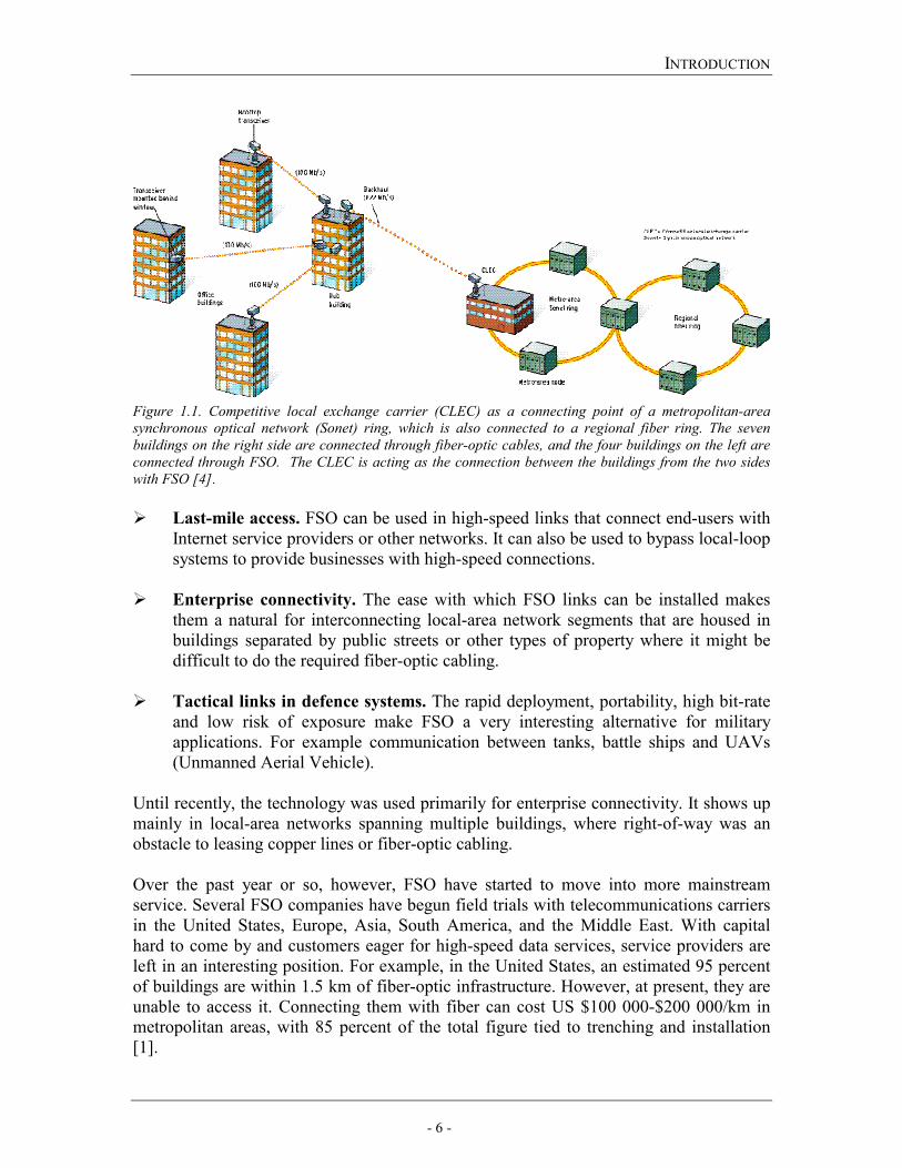
1.1.2 Applications FSO-links can be advantageous in various situations. We have stated below the applications we believe are the most important: Metro network extensions. Carriers can deploy FSO to extend existing
metropolitan-area fiber rings to connect new networks in their core infrastructure, or to complete Sonet rings, see Figure 1.1.
INTRODUCTION
- 6 -
Figure 1.1. Competitive local exchange carrier (CLEC) as a connecting point of a metropolitan-area synchronous optical network (Sonet) ring, which is also connected to a regional fiber ring. The seven buildings on the right side are connected through fiber-optic cables, and the four buildings on the left are connected through FSO. The CLEC is acting as the connection between the buildings from the two sides with FSO [4]. Last-mile access. FSO can be used in high-speed links that connect end-users with
Internet service providers or other networks. It can also be used to bypass local-loop systems to provide businesses with high-speed connections.
Enterprise connectivity. The ease with which FSO links can be installed makes
them a natural for interconnecting local-area network segments that are housed in buildings separated by public streets or other types of property where it might be difficult to do the required fiber-optic cabling.
Tactical links in defence systems. The rapid deployment, portability, high bit-rate
and low risk of exposure make FSO a very interesting alternative for military applications. For example communication between tanks, battle ships and UAVs (Unmanned Aerial Vehicle).
Until recently, the technology was used primarily for enterprise connectivity. It shows up mainly in local-area networks spanning multiple buildings, where right-of-way was an obstacle to leasing copper lines or fiber-optic cabling. Over the past year or so, however, FSO have started to move into more mainstream service. Several FSO companies have begun field trials with telecommunications carriers in the United States, Europe, Asia, South America, and the Middle East. With capital hard to come by and customers eager for high-speed data services, service providers are left in an interesting position. For example, in the United States, an estimated 95 percent of buildings are within 1.5 km of fiber-optic infrastructure. However, at present, they are unable to access it. Connecting them with fiber can cost US $100 000-$200 000/km in metropolitan areas, with 85 percent of the total figure tied to trenching and installation [1].
INTRODUCTION
- 7 -
1.1.3 Advantages and disadvantages Advantages
++++ Cost
FSO links greatest advantages are their low cost per bit and time to market. In most cases, FSO is an attractive alternative to the prohibitive cost of trenching the streets to lay fiber, the logistical complexity of obtaining right-of-way permits, or the recurrent costs of leasing fiber lines. For example, one mile fiber deployment in urban areas could cost $300,000-$700,000 given the cost involved in digging tunnels and getting right-of-way. A fixed RF wireless solution could cost $30,000. By contrast, a short FSO link of 155 Mbs might cost only $ 18,000 [5].
++++ Transmission rate Radio frequency (RF) can transmit data much farther than FSO, but its bandwidth is limited to 622 Mb/s. Available FSO systems provide a bandwidth of up to 2.7 Gb/s. 160 Gb/s has been successfully tested in laboratories; speeds could potentially be able to reach into the Terabit range [2, 6, 36].
++++ Installation
Compared to fiber communication FSO does not require digging and permission from authorities for installation. FSO only needs a place on a roof or a place behind a window to set up its transceiver to transmit and to receive data. Installation can be made over the day.
++++ Licensing A major advantage of FSO over Radio Frequency (RF) is that no Federal Communications Commission (FCC) licensing or frequency allocating is required. This is because frequencies greater than 300 GHz (less than 1 mm in wavelength) are unregulated. In some urban areas or near airports it is very difficult and costly to obtain frequency allocation for microwave transmission. In addition, the potential customer base is not limited to frequency license holders.
++++ Portability FSO terminals are portable and quickly deployable, which for example make them suitable for disaster recovery (e.g. FSO was frequently applied in New York after the 11th of September) and temporary installations.
++++ Security
The narrow beam of the laser makes detection, interception and jamming very difficult. The FSO-systems are normally installed as high as possible so that passing cars; trucks or other moving things do not interfere with the beam. Beam tapping would require that a mirror or other device remain in the beam path for extended periods. Care would need to be taken by the intruder not to disrupt the transmission
INTRODUCTION
- 8 -
path of either beam because if one beam is interrupted this is immediately noticed by the users of the system. Further, the other beam would automatically go into failure recovery mode and would not transmit any data of interest to the intruder. Because of its superior security, compared to RF-transmission, FSO is suitable for transfer of financial, legal, military or other sensitive information [6].
Disadvantages FSO does have its share of limitations. As a ‘line of sight’ technology, FSO is vulnerable to the severance of connections because of bad weather and other factors discussed below:
−−−− Poor weather
One of the biggest barriers that this technology faces is the effect of weather conditions on signal transmission. This limitation makes FSO suitable only for short distance communication. An off-the-shelf FSO-system has a maximal range of approximately 500 m when thick fog reduces the visibility to only 200 m. Fog represents the greatest challenge, as the water particles are small and dense enough to diffract the light pulse and extinct the signal. Since the particles of rain and snowfall are large compared to the used wavelength, they affect the transmission less than fog [7].
−−−− Physical obstructions
Since FSO requires a free line of sight, a pre-installation site evaluation must be done to ensure that the paths between the FSO units are clear and will remain so for a long time. The growth of trees and the construction of buildings need to be considered. Birds can block the beam temporarily. If a bird (or any other object) crosses the beam the data transmission will be momentarily interrupted. Ethernet and Token ring can handle such interrupts and will retransmit the data as per protocol [8].
−−−− Building movements
Building movement caused by environmental conditions such as wind can upset the receiver and transmitter alignment.
−−−− Scintillations
Heated air rising from the ground or rooftops creates temperature variations among different air pockets. As a consequence, the refractive index may vary in a time dependent and randomness manner along the line of sight of the link, giving rise to scintillations over the beam cross section. These scintillations appear as power fluctuation in the receiver [9].
INTRODUCTION
- 9 -
1.2 The thesis assignment The thesis assignment was originally specified by Ericsson Research in Kista, Stockholm, but was performed and supervised in collaboration with the Swedish Defence Research Agency (FOI) in Linköping. The workplace of the master thesis has been at FOI, since necessary equipment and premises for the laboratory and field tests were readily available. The master thesis is concluded in a written report and an oral presentation at Ericsson Research in Kista, FOI in Linköping and the University of Linköping.
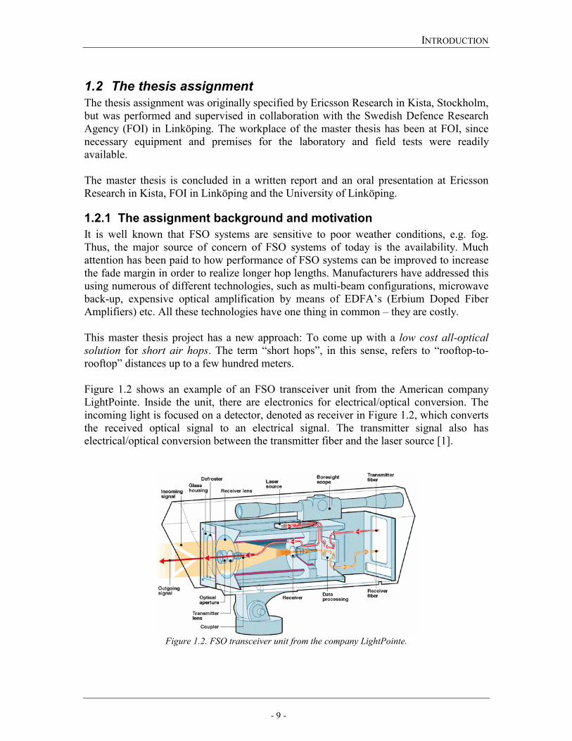
1.2.1 The assignment background and motivation It is well known that FSO systems are sensitive to poor weather conditions, e.g. fog. Thus, the major source of concern of FSO systems of today is the availability. Much attention has been paid to how performance of FSO systems can be improved to increase the fade margin in order to realize longer hop lengths. Manufacturers have addressed this using numerous of different technologies, such as multi-beam configurations, microwave back-up, expensive optical amplification by means of EDFA’s (Erbium Doped Fiber Amplifiers) etc. All these technologies have one thing in common – they are costly. This master thesis project has a new approach: To come up with a low cost all-optical solution for short air hops. The term “short hops”, in this sense, refers to “rooftop-to-rooftop” distances up to a few hundred meters. Figure 1.2 shows an example of an FSO transceiver unit from the American company LightPointe. Inside the unit, there are electronics for electrical/optical conversion. The incoming light is focused on a detector, denoted as receiver in Figure 1.2, which converts the received optical signal to an electrical signal. The transmitter signal also has electrical/optical conversion between the transmitter fiber and the laser source [1].
Figure 1.2. FSO transceiver unit from the company LightPointe.
INTRODUCTION
- 10 -
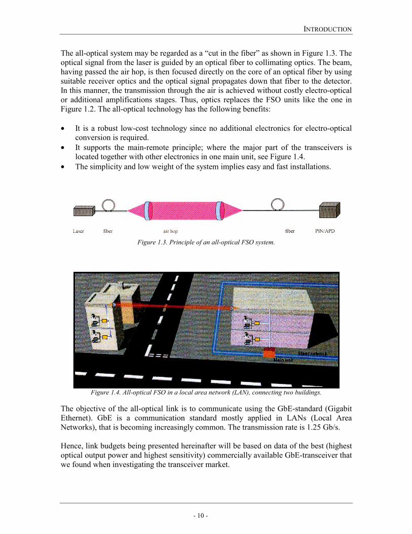
The all-optical system may be regarded as a “cut in the fiber” as shown in Figure 1.3. The optical signal from the laser is guided by an optical fiber to collimating optics. The beam, having passed the air hop, is then focused directly on the core of an optical fiber by using suitable receiver optics and the optical signal propagates down that fiber to the detector. In this manner, the transmission through the air is achieved without costly electro-optical or additional amplifications stages. Thus, optics replaces the FSO units like the one in Figure 1.2. The all-optical technology has the following benefits: • It is a robust low-cost technology since no additional electronics for electro-optical
conversion is required. • It supports the main-remote principle; where the major part of the transceivers is
located together with other electronics in one main unit, see Figure 1.4. • The simplicity and low weight of the system implies easy and fast installations.
Figure 1.3. Principle of an all-optical FSO system.
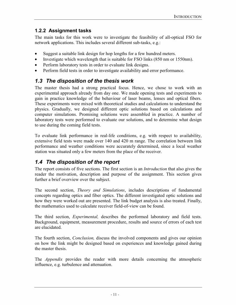
Figure 1.4. All-optical FSO in a local area network (LAN), connecting two buildings.
The objective of the all-optical link is to communicate using the GbE-standard (Gigabit Ethernet). GbE is a communication standard mostly applied in LANs (Local Area Networks), that is becoming increasingly common. The transmission rate is 1.25 Gb/s. Hence, link budgets being presented hereinafter will be based on data of the best (highest optical output power and highest sensitivity) commercially available GbE-transceiver that we found when investigating the transceiver market.
INTRODUCTION
- 11 -
1.2.2 Assignment tasks The main tasks for this work were to investigate the feasibility of all-optical FSO for network applications. This includes several different sub-tasks, e.g.: • Suggest a suitable link design for hop lengths for a few hundred meters. • Investigate which wavelength that is suitable for FSO links (850 nm or 1550nm). • Perform laboratory tests in order to evaluate link designs. • Perform field tests in order to investigate availability and error performance.
1.3 The disposition of the thesis work The master thesis had a strong practical focus. Hence, we chose to work with an experimental approach already from day one. We made opening tests and experiments to gain in practice knowledge of the behaviour of laser beams, lenses and optical fibers. These experiments were mixed with theoretical studies and calculations to understand the physics. Gradually, we designed different optic solutions based on calculations and computer simulations. Promising solutions were assembled in practice. A number of laboratory tests were performed to evaluate our solutions, and to determine what design to use during the coming field tests. To evaluate link performance in real-life conditions, e.g. with respect to availability, extensive field tests were made over 140 and 420 m range. The correlation between link performance and weather conditions were accurately determined, since a local weather station was situated only a few meters from the place of the receiver.
1.4 The disposition of the report The report consists of five sections. The first section is an Introduction that also gives the reader the motivation, description and purpose of the assignment. This section gives further a brief overview over the subject. The second section, Theory and Simulations, includes descriptions of fundamental concepts regarding optics and fiber optics. The different investigated optic solutions and how they were worked out are presented. The link budget analysis is also treated. Finally, the mathematics used to calculate receiver field-of-view can be found. The third section, Experimental, describes the performed laboratory and field tests. Background, equipment, measurement procedure, results and source of errors of each test are elucidated. The fourth section, Conclusion, discuss the involved components and gives our opinion on how the link might be designed based on experiences and knowledge gained during the master thesis. The Appendix provides the reader with more details concerning the atmospheric influence, e.g. turbulence and attenuation.
THEORY AND SIMULATIONS
- 12 -
2 Theory and simulations
2.1 Fundamental optics and fiber optics In this Section, we will briefly introduce some optical properties that we refer to throughout the report.
2.1.1 Diffraction Diffraction is a natural property of light due to its wave nature, and possesses a fundamental limitation on any optical system. Diffraction is always present, although its effects may be masked if the system has significant aberrations. When a lens, mirror or an entire optical system is made to be essentially free from aberration its performance is limited only by diffraction, and is thereby called diffraction-limited [10].
2.1.2 Chromatic Aberration The index of refraction of a material is a function of wavelength. This is known as dispersion. Consequently, light rays of different wavelengths will be refracted at different angles. Typically, the index of refraction is higher for shorter wavelengths. Therefore, shorter wavelengths are focused closer to the lens than the longer wavelengths. Longitudinal chromatic aberration is defined as the axial distance from the nearest to the farthest focal point [11].
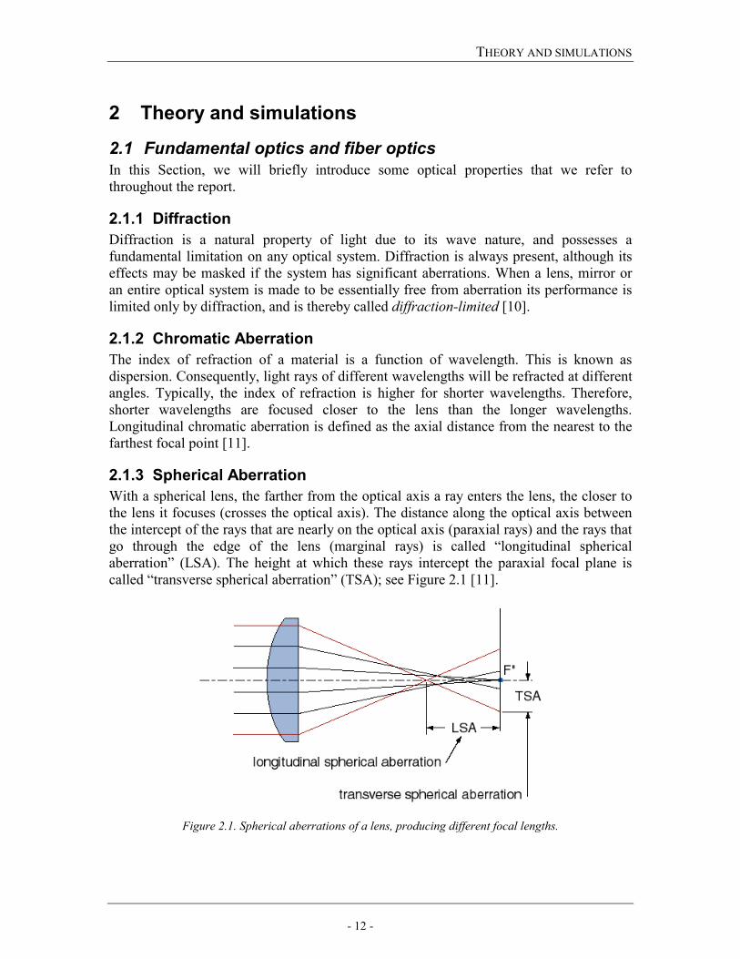
2.1.3 Spherical Aberration With a spherical lens, the farther from the optical axis a ray enters the lens, the closer to the lens it focuses (crosses the optical axis). The distance along the optical axis between the intercept of the rays that are nearly on the optical axis (paraxial rays) and the rays that go through the edge of the lens (marginal rays) is called “longitudinal spherical aberration” (LSA). The height at which these rays intercept the paraxial focal plane is called “transverse spherical aberration” (TSA); see Figure 2.1 [11].
Figure 2.1. Spherical aberrations of a lens, producing different focal lengths.
THEORY AND SIMULATIONS
- 13 -
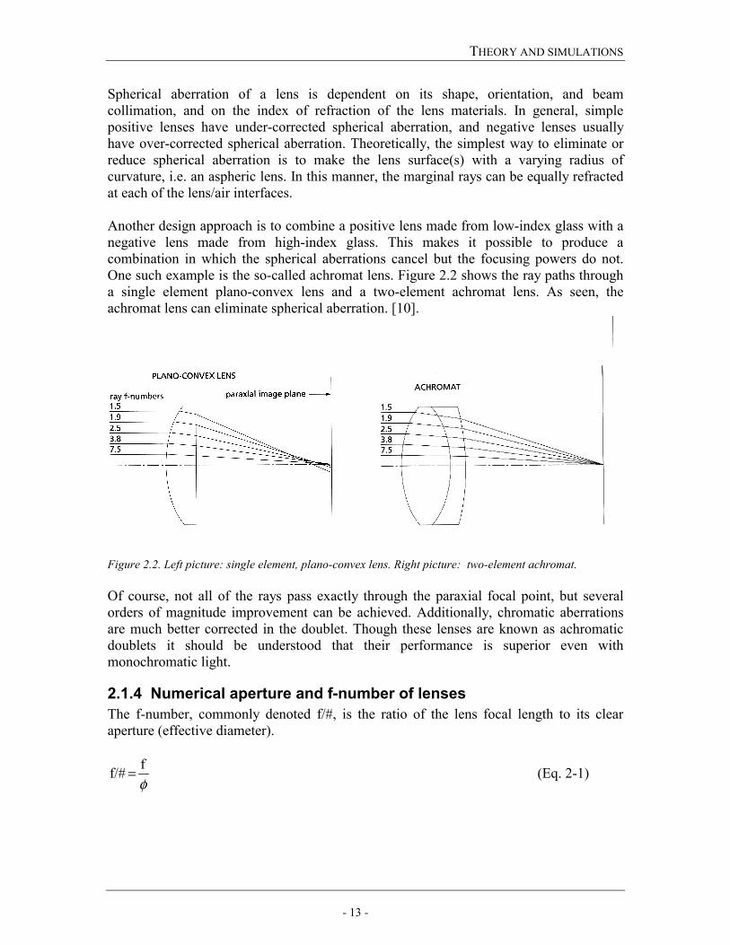
Spherical aberration of a lens is dependent on its shape, orientation, and beam collimation, and on the index of refraction of the lens materials. In general, simple positive lenses have under-corrected spherical aberration, and negative lenses usually have over-corrected spherical aberration. Theoretically, the simplest way to eliminate or reduce spherical aberration is to make the lens surface(s) with a varying radius of curvature, i.e. an aspheric lens. In this manner, the marginal rays can be equally refracted at each of the lens/air interfaces. Another design approach is to combine a positive lens made from low-index glass with a negative lens made from high-index glass. This makes it possible to produce a combination in which the spherical aberrations cancel but the focusing powers do not. One such example is the so-called achromat lens. Figure 2.2 shows the ray paths through a single element plano-convex lens and a two-element achromat lens. As seen, the achromat lens can eliminate spherical aberration. [10].
Figure 2.2. Left picture: single element, plano-convex lens. Right picture: two-element achromat. Of course, not all of the rays pass exactly through the paraxial focal point, but several orders of magnitude improvement can be achieved. Additionally, chromatic aberrations are much better corrected in the doublet. Though these lenses are known as achromatic doublets it should be understood that their performance is superior even with monochromatic light.
2.1.4 Numerical aperture and f-number of lenses The f-number, commonly denoted f/#, is the ratio of the lens focal length to its clear aperture (effective diameter).
φf f/# = (Eq. 2-1)
THEORY AND SIMULATIONS
- 14 -
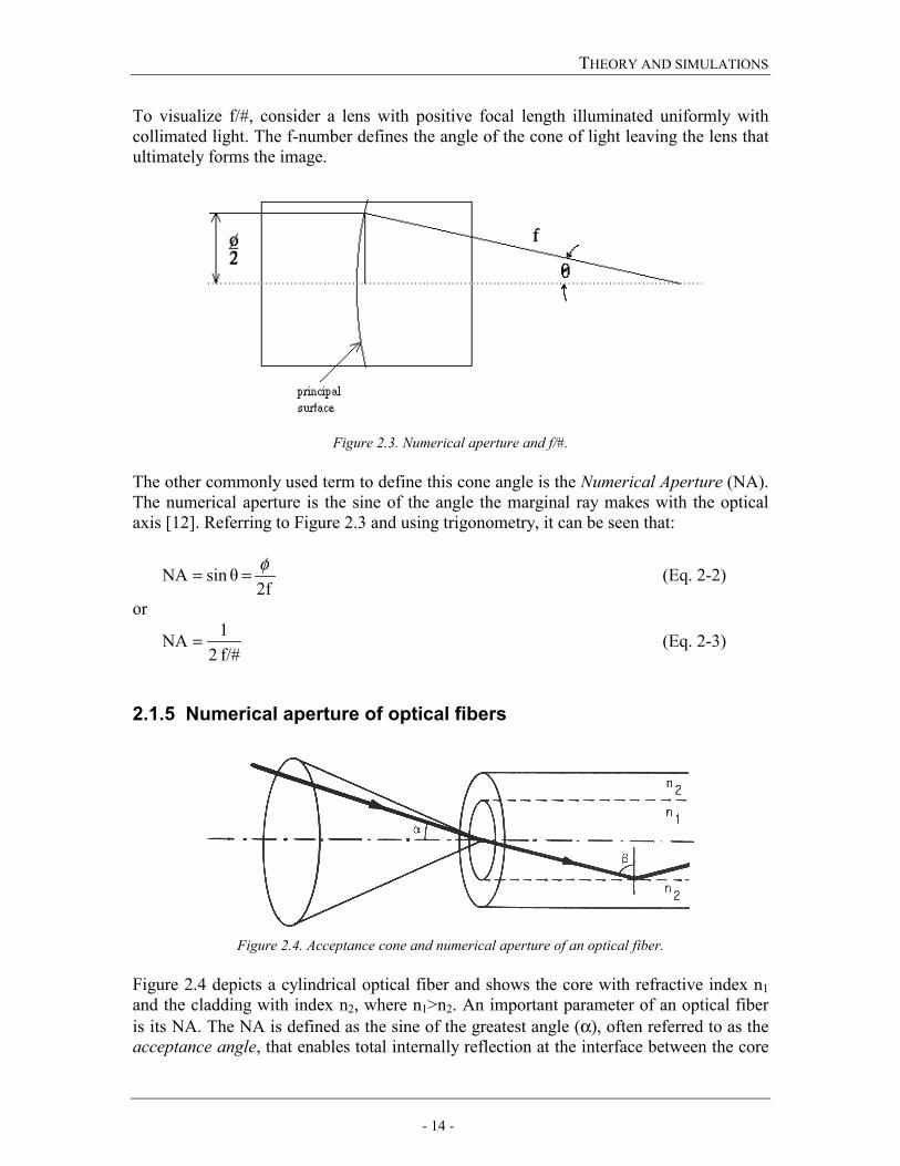
To visualize f/#, consider a lens with positive focal length illuminated uniformly with collimated light. The f-number defines the angle of the cone of light leaving the lens that ultimately forms the image.
Figure 2.3. Numerical aperture and f/#. The other commonly used term to define this cone angle is the Numerical Aperture (NA). The numerical aperture is the sine of the angle the marginal ray makes with the optical axis [12]. Referring to Figure 2.3 and using trigonometry, it can be seen that:
2f
θsinNA φ== (Eq. 2-2)
or
f/# 21NA = (Eq. 2-3)
2.1.5 Numerical aperture of optical fibers
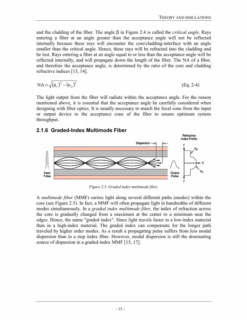
Figure 2.4. Acceptance cone and numerical aperture of an optical fiber.
Figure 2.4 depicts a cylindrical optical fiber and shows the core with refractive index n1 and the cladding with index n2, where n1>n2. An important parameter of an optical fiber is its NA. The NA is defined as the sine of the greatest angle (α), often referred to as the acceptance angle, that enables total internally reflection at the interface between the core
THEORY AND SIMULATIONS
- 15 -
and the cladding of the fiber. The angle β in Figure 2.4 is called the critical angle. Rays entering a fiber at an angle greater than the acceptance angle will not be reflected internally because these rays will encounter the core/cladding-interface with an angle smaller than the critical angle. Hence, these rays will be refracted into the cladding and be lost. Rays entering a fiber at an angle equal to or less than the acceptance angle will be reflected internally, and will propagate down the length of the fiber. The NA of a fiber, and therefore the acceptance angle, is determined by the ratio of the core and cladding refractive indices [13, 14].
( ) ( )22
21 nn NA −= (Eq. 2-4)
The light output from the fiber will radiate within the acceptance angle. For the reason mentioned above, it is essential that the acceptance angle be carefully considered when designing with fiber optics. It is usually necessary to match the focal cone from the input or output device to the acceptance cone of the fiber to ensure optimum system throughput.
2.1.6 Graded-Index Multimode Fiber
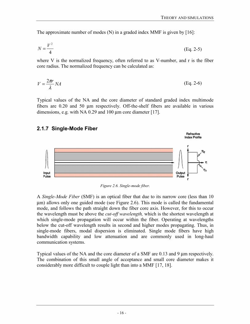
Figure 2.5. Graded index multimode fiber.
A multimode fiber (MMF) carries light along several different paths (modes) within the core (see Figure 2.5). In fact, a MMF will often propagate light in hundredths of different modes simultaneously. In a graded index multimode fiber, the index of refraction across the core is gradually changed from a maximum at the center to a minimum near the edges. Hence, the name "graded index". Since light travels faster in a low-index material than in a high-index material. The graded index can compensate for the longer path traveled by higher order modes. As a result a propagating pulse suffers from less modal dispersion than in a step index fiber. However, modal dispersion is still the dominating source of dispersion in a graded-index MMF [15, 17].
THEORY AND SIMULATIONS
- 16 -
NArV
VN
λπ2
4
2
=
=
The approximate number of modes (N) in a graded index MMF is given by [16]:
(Eq. 2-5) where V is the normalized frequency, often referred to as V-number, and r is the fiber core radius. The normalized frequency can be calculated as:
(Eq. 2-6) Typical values of the NA and the core diameter of standard graded index multimode fibers are 0.20 and 50 µm respectively. Off-the-shelf fibers are available in various dimensions, e.g. with NA 0.29 and 100 µm core diameter [17].
2.1.7 Single-Mode Fiber
Figure 2.6. Single-mode fiber.
A Single-Mode Fiber (SMF) is an optical fiber that due to its narrow core (less than 10 µm) allows only one guided mode (see Figure 2.6). This mode is called the fundamental mode, and follows the path straight down the fiber core axis. However, for this to occur the wavelength must be above the cut-off wavelength, which is the shortest wavelength at which single-mode propagation will occur within the fiber. Operating at wavelengths below the cut-off wavelength results in second and higher modes propagating. Thus, in single-mode fibers, modal dispersion is eliminated. Single mode fibers have high bandwidth capability and low attenuation and are commonly used in long-haul communication systems. Typical values of the NA and the core diameter of a SMF are 0.13 and 9 µm respectively. The combination of this small angle of acceptance and small core diameter makes it considerably more difficult to couple light than into a MMF [17, 18].
THEORY AND SIMULATIONS
- 17 -
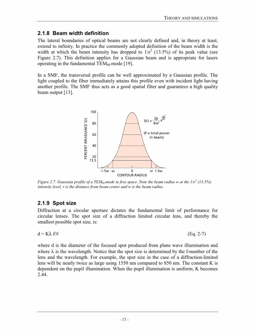
2.1.8 Beam width definition The lateral boundaries of optical beams are not clearly defined and, in theory at least, extend to infinity. In practice the commonly adopted definition of the beam width is the width at which the beam intensity has dropped to 1/e2 (13.5%) of its peak value (see Figure 2.7). This definition applies for a Gaussian beam and is appropriate for lasers operating in the fundamental TEM00 mode [19]. In a SMF, the transversal profile can be well approximated by a Gaussian profile. The light coupled to the fiber immediately attains this profile even with incident light having another profile. The SMF thus acts as a good spatial filter and guarantees a high quality beam output [13].
Figure 2.7. Gaussian profile of a TEM00 mode in free space. Note the beam radius w at the 1/e2 (13.5%) intensity level, r is the distance from beam center and w is the beam radius.
2.1.9 Spot size Diffraction at a circular aperture dictates the fundamental limit of performance for circular lenses. The spot size of a diffraction limited circular lens, and thereby the smallest possible spot size, is: d = Kλ f/# (Eq. 2-7) where d is the diameter of the focused spot produced from plane wave illumination and where λ is the wavelength. Notice that the spot size is determined by the f-number of the lens and the wavelength. For example, the spot size in the case of a diffraction-limited lens will be nearly twice as large using 1550 nm compared to 850 nm. The constant K is dependent on the pupil illumination. When the pupil illumination is uniform, K becomes 2.44.
THEORY AND SIMULATIONS
- 18 -
To decide whether the pupil illumination can be approximated to be uniform when having a Gaussian output beam it is helpful to introduce the truncation ratio, T:
t
b
DD
T = (Eq. 2-8)
where Db is the Gaussian beam diameter measured at 1/e2 intensity point and Dt is the limiting aperture diameter of the lens. If T > 2 uniform illumination can be assumed and the image spot also takes on a uniform illumination and its size can thereby be determined without any truncation. If T = 1 the spot profile will be a hybrid between uniform and Gaussian distribution. When T = 0.5 the spot intensity profile approaches a Gaussian distribution. Calculations of the spot size for truncation ratios less than two (T < 2) requires that K be evaluated. This is done, at the 1/e2 (13.5 %) intensity point, using the formula [11, 19]
( ) ( ) 891.1821.1/1 2816.05320.0
2816.06460.06449.12
−−
−+=
TTK e (Eq. 2-9)
For example, if T = 1 then K1/e
2 becomes 1.83. Instead, if spherical aberrations dominate (e.g. commonly when using a plano-convex singlet lens), and hence state the limitation in spot size, Equation 2-10 applies. However, Equation 2-10 is valid only in the case of monochromatic spherical aberration of a plano-convex lens and an approximately plane incident wavefront.
aberration spherical todue sizespot The is [11]:
3f/#0.067f d = (Eq. 2-10)
Since, in the case of one spherical lens, the diffraction increases and aberrations decrease with increasing f-number, determining optimum system performance often involves finding a point where the combination of these factors has a minimum effect [11].
2.1.10 Fresnel reflection Fresnel reflection is the reflection of a portion of the incident light at an interface between two media having different refractive indices.
For a normal wave, the fraction of reflected incident power is given by the equation [16]:
( )( )2
21
221
nnnnR
+−
= (Eq. 2-11)
THEORY AND SIMULATIONS
- 19 -
where R is the reflection coefficient and n1 and n2 are the respective refractive indices of the two media. With n1 = 1 (refractive index for air) and n2 = 1.5 (refractive index for the glass of current interest) this yields:
( )( )
04.05.115.11
2
2
=+−=R
Hence, it exists a transmission loss on the order of 4 % per glass-air interface due to Fresnel reflections.
2.1.11 Antireflection coatings Fresnel reflections can be reduced considerably by coating the optical components with antireflection coatings. The antireflection coatings consist of one or more dielectric thin-film layers having a specific refractive index and thickness [10].
2.2 Investigated optics This section gives a brief overview of our optical design procedure and the used computer software Zemax (Version: January 2 2002, Focus Software). Moreover, some important factors to consider when selecting transmitter and receiver optics are discussed. To investigate possible solutions for the transmitter and receiver optics suitable for our FSO-link we performed a number of calculations and simulations. Ray tracing formulas were used to determine the optical characteristics of some potential lens systems, e.g. a single lens coupler, Keplerian telescope and the Cassegrain telescope. To verify our analytical expressions simulations using a computer aided design tool called Zemax were made. Zemax is a program that can model, analyze and assist in the design of optical systems. One of many useful features is that Zemax includes an up to date lens catalog with the most common vendors lens assortment. Thereby, the performance of off-the-shelf lenses can be investigated. Another particular feature of great use in our case was that the encircled energy at the image plane could be calculated. Since values of the circle diameter and NA can be set, this feature is of great benefit when calculating the coupling efficiency for different lens systems and fibers.
2.2.1 Transmitter optics The main purpose of the transmitter optics is to produce a suitable beam divergence matching a desired beam diameter at the receiver. Without transmitter optics the beam divergence would be the same as the acceptance angle of the used fiber, 0.20 rad in the MMF-case and 0.13 rad in the SMF-case, leading to a beam diameter of 200 and 130 m respectively at a distance of 500 m. Clearly this divergence is too large. Moreover, a desired feature of the transmitter optics is that it should add a minimum of spherical aberrations. The final spot size will be affected by these aberrations. We have used a diffraction-limited lens to ensure a minimum spot size as regards to the transmitter.
THEORY AND SIMULATIONS
- 20 -
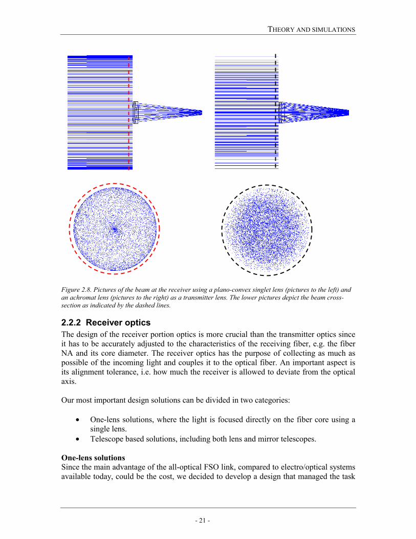
When the light is transmitted through a SMF, it has approximately a Gaussian profile when leaving the fiber. It is desirable to preserve this profile along the path of propagation in the air of several reasons; knowing that the maximal power density is situated in the beam center makes alignment easier, high intensity around the beam edges is avoided and finally it makes it easier to calculate the energy encircled by the receiver aperture. Figure 2.8 shows the results of simulations of two different transmitter lenses made in Zemax. The left side depicts the beam at the receiver after being transmitted using a plano-convex singlet lens (diameter = 20 mm) and the right side when using a diffraction limited achromat lens (diameter = 20 mm). The beam at the receiver is 26 cm in both cases and the number of simulated rays is the same. The path of propagation was set to 200 m. A considerable difference in ray distribution between the two cases is seen. In the achromat case the ray distribution is dense in the middle of the beam, and decrease towards the beam edges. Consequently, a relatively large fraction of the rays falls on the receiver aperture. The plano-convex singlet lens on the other hand does not manage to preserve the Gaussian profile resulting in a lower fraction of the rays hitting the receiver aperture. The two lower pictures show the beam cross-sections as indicated by the dashed lines. An important observation regarding fiber coupling was that the achromat as a transmitter lens resulted in a diffraction limited spot size. As expected, the achromat did not add spherical aberrations. On the other hand when introducing the singlet lens as a transmitter lens, the spot size increased to twice the original size. Another interesting observation was that the plano-convex singlet is not able to collimate the beam as well as the achromat. The smallest possible beam diameter was 26 cm after 200 m propagation, which yields 65 cm after 500 m, whereas the achromat completely collimated the beam (same beam diameter at receiver and transmitter). Worth remembering is that Zemax does not consider beam divergence due to diffraction and hence the observed difference between the lenses is only due to their ability to refract the rays.
THEORY AND SIMULATIONS
- 21 -
Figure 2.8. Pictures of the beam at the receiver using a plano-convex singlet lens (pictures to the left) and an achromat lens (pictures to the right) as a transmitter lens. The lower pictures depict the beam cross-section as indicated by the dashed lines.
2.2.2 Receiver optics The design of the receiver portion optics is more crucial than the transmitter optics since it has to be accurately adjusted to the characteristics of the receiving fiber, e.g. the fiber NA and its core diameter. The receiver optics has the purpose of collecting as much as possible of the incoming light and couples it to the optical fiber. An important aspect is its alignment tolerance, i.e. how much the receiver is allowed to deviate from the optical axis. Our most important design solutions can be divided in two categories:
• One-lens solutions, where the light is focused directly on the fiber core using a single lens.
• Telescope based solutions, including both lens and mirror telescopes. One-lens solutions Since the main advantage of the all-optical FSO link, compared to electro/optical systems available today, could be the cost, we decided to develop a design that managed the task
THEORY AND SIMULATIONS
- 22 -
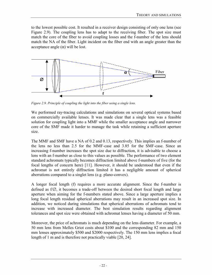
to the lowest possible cost. It resulted in a receiver design consisting of only one lens (see Figure 2.9). The coupling lens has to adapt to the receiving fiber. The spot size must match the core of the fiber to avoid coupling losses and the f-number of the lens should match the NA of the fiber. Light incident on the fiber end with an angle greater than the acceptance angle (α) will be lost. Figure 2.9. Principle of coupling the light into the fiber using a single lens. We performed ray-tracing calculations and simulations on several optical systems based on commercially available lenses. It was made clear that a single lens was a feasible solution for coupling light into a MMF while the smaller acceptance angle and narrower core of the SMF made it harder to manage the task while retaining a sufficient aperture size. The MMF and SMF have a NA of 0.2 and 0.13, respectively. This implies an f-number of the lens no less than 2.5 for the MMF-case and 3.85 for the SMF-case. Since an increasing f-number increases the spot size due to diffraction, it is advisable to choose a lens with an f-number as close to this values as possible. The performance of two element standard achromats typically becomes diffraction limited above f-numbers of five (for the focal lengths of concern here) [11]. However, it should be understood that even if the achromat is not entirely diffraction limited it has a negligible amount of spherical aberrations compared to a singlet lens (e.g. plano-convex). A longer focal length (f) requires a more accurate alignment. Since the f-number is defined as f/∅, it becomes a trade-off between the desired short focal length and large aperture when aiming for the f-numbers stated above. Since a large aperture implies a long focal length residual spherical aberrations may result in an increased spot size. In addition, we noticed during simulations that spherical aberrations of achromats tend to increase with increased diameter. The best simulation results regarding alignment tolerances and spot size were obtained with achromat lenses having a diameter of 50 mm. Moreover, the price of achromats is much depending on the lens diameter. For example, a 50 mm lens from Melles Griot costs about $100 and the corresponding 82 mm and 150 mm lenses approximately $500 and $2000 respectively. The 150 mm lens implies a focal length of 1 m and is therefore not practically viable [20, 24].
αααα Fiber
f
∅∅∅∅
THEORY AND SIMULATIONS
- 23 -
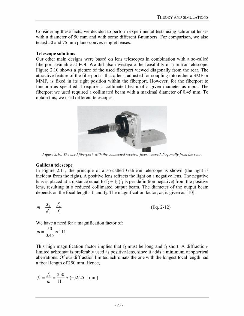
Considering these facts, we decided to perform experimental tests using achromat lenses with a diameter of 50 mm and with some different f-numbers. For comparison, we also tested 50 and 75 mm plano-convex singlet lenses. Telescope solutions Our other main designs were based on lens telescopes in combination with a so-called fiberport available at FOI. We did also investigate the feasibility of a mirror telescope. Figure 2.10 shows a picture of the used fiberport viewed diagonally from the rear. The attractive feature of the fiberport is that a lens, adjusted for coupling into either a SMF or MMF, is fixed in its right position within the fiberport. However, for the fiberport to function as specified it requires a collimated beam of a given diameter as input. The fiberport we used required a collimated beam with a maximal diameter of 0.45 mm. To obtain this, we used different telescopes.
Figure 2.10. The used fiberport, with the connected receiver fiber, viewed diagonally from the rear.
Galilean telescope In Figure 2.11, the principle of a so-called Galilean telescope is shown (the light is incident from the right). A positive lens refracts the light on a negative lens. The negative lens is placed at a distance equal to f2 + f1 (f1 is per definition negative) from the positive lens, resulting in a reduced collimated output beam. The diameter of the output beam depends on the focal lengths f1 and f2. The magnification factor, m, is given as [10]:
1
2
1
2
ff
ddm == (Eq. 2-12)
We have a need for a magnification factor of:
11145.0
50 ≈=m
This high magnification factor implies that f2 must be long and f1 short. A diffraction-limited achromat is preferably used as positive lens, since it adds a minimum of spherical aberrations. Of our diffraction limited achromats the one with the longest focal length had a focal length of 250 mm. Hence,
25.2)(1112502
1 −≈==mff [mm]
THEORY AND SIMULATIONS
- 24 -
We were not able to find a negative lens with such short focal length, and did never realize this design. However, if a suitable negative lens, preferably a diffraction limited, can be found this telescope is a possible alternative.
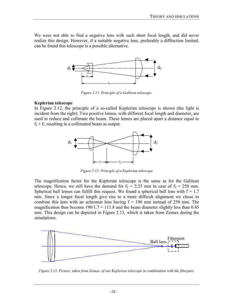
Figure 2.11. Principle of a Galilean telescope. Keplerian telescope In Figure 2.12, the principle of a so-called Keplerian telescope is shown (the light is incident from the right). Two positive lenses, with different focal length and diameter, are used to reduce and collimate the beam. These lenses are placed apart a distance equal to f2 + f1, resulting in a collimated beam as output.
Figure 2.12. Principle of a Keplerian telescope The magnification factor for the Keplerian telescope is the same as for the Galilean telescope. Hence, we still have the demand for f2 = 2.25 mm in case of f2 = 250 mm. Spherical ball lenses can fulfill this request. We found a spherical ball lens with f = 1.7 mm. Since a longer focal length give rise to a more difficult alignment we chose to combine this lens with an achromat lens having f = 190 mm instead of 250 mm. The magnification thus become 190/1.7 = 111.8 and the beam diameter slightly less than 0.45 mm. This design can be depicted in Figure 2.13, which is taken from Zemax during the simulations.
Figure 2.13. Picture, taken from Zemax, of our Keplerian telescope in combination with the fiberport.
d2d1
Fiberport Ball lens
d2d1
THEORY AND SIMULATIONS
- 25 -
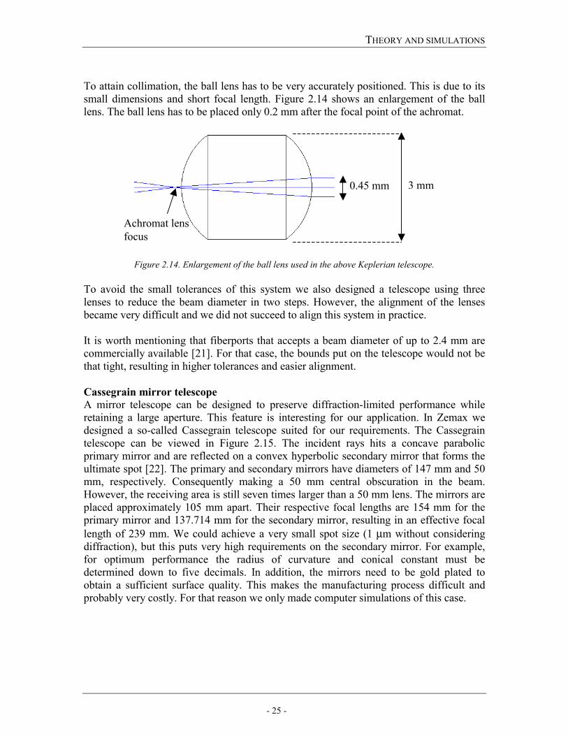
To attain collimation, the ball lens has to be very accurately positioned. This is due to its small dimensions and short focal length. Figure 2.14 shows an enlargement of the ball lens. The ball lens has to be placed only 0.2 mm after the focal point of the achromat.
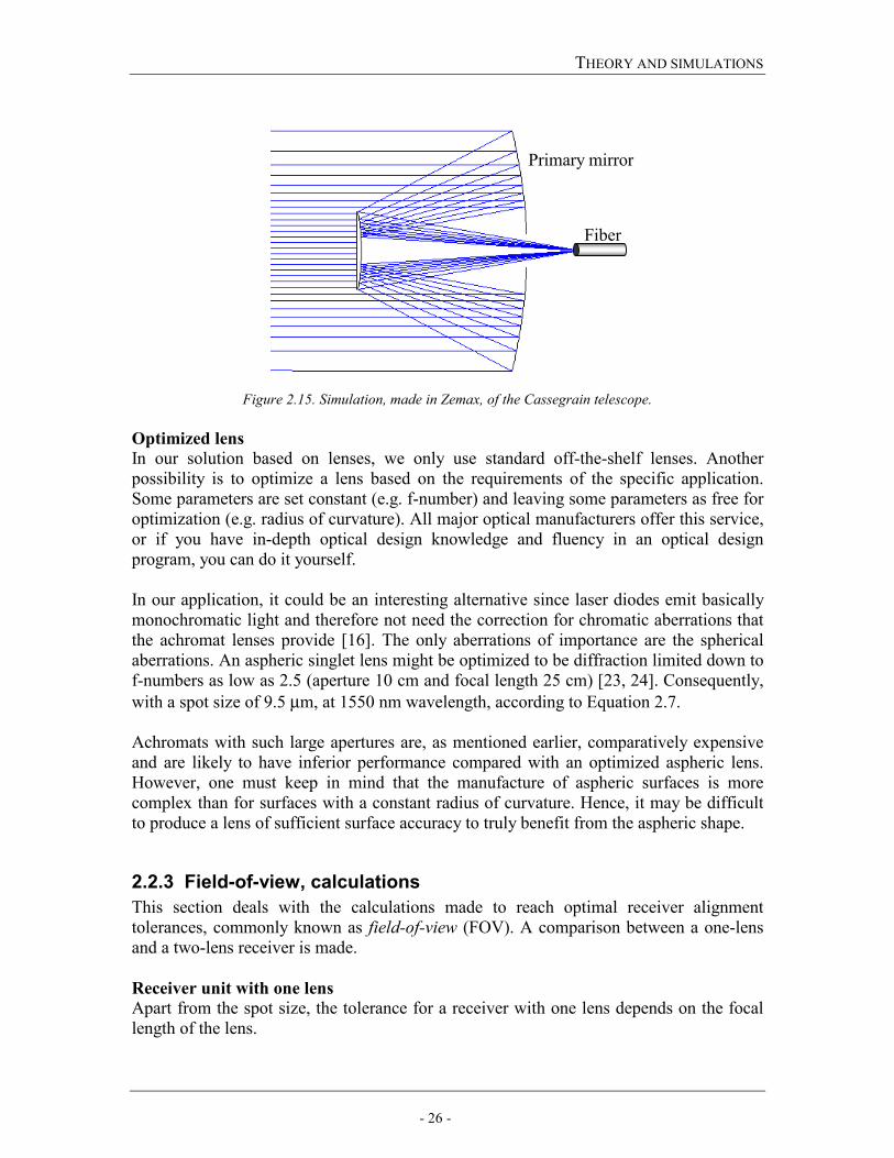
Figure 2.14. Enlargement of the ball lens used in the above Keplerian telescope. To avoid the small tolerances of this system we also designed a telescope using three lenses to reduce the beam diameter in two steps. However, the alignment of the lenses became very difficult and we did not succeed to align this system in practice. It is worth mentioning that fiberports that accepts a beam diameter of up to 2.4 mm are commercially available [21]. For that case, the bounds put on the telescope would not be that tight, resulting in higher tolerances and easier alignment. Cassegrain mirror telescope A mirror telescope can be designed to preserve diffraction-limited performance while retaining a large aperture. This feature is interesting for our application. In Zemax we designed a so-called Cassegrain telescope suited for our requirements. The Cassegrain telescope can be viewed in Figure 2.15. The incident rays hits a concave parabolic primary mirror and are reflected on a convex hyperbolic secondary mirror that forms the ultimate spot [22]. The primary and secondary mirrors have diameters of 147 mm and 50 mm, respectively. Consequently making a 50 mm central obscuration in the beam. However, the receiving area is still seven times larger than a 50 mm lens. The mirrors are placed approximately 105 mm apart. Their respective focal lengths are 154 mm for the primary mirror and 137.714 mm for the secondary mirror, resulting in an effective focal length of 239 mm. We could achieve a very small spot size (1 µm without considering diffraction), but this puts very high requirements on the secondary mirror. For example, for optimum performance the radius of curvature and conical constant must be determined down to five decimals. In addition, the mirrors need to be gold plated to obtain a sufficient surface quality. This makes the manufacturing process difficult and probably very costly. For that reason we only made computer simulations of this case.
3 mm 0.45 mm
Achromat lens focus
THEORY AND SIMULATIONS
- 26 -
Figure 2.15. Simulation, made in Zemax, of the Cassegrain telescope. Optimized lens In our solution based on lenses, we only use standard off-the-shelf lenses. Another possibility is to optimize a lens based on the requirements of the specific application. Some parameters are set constant (e.g. f-number) and leaving some parameters as free for optimization (e.g. radius of curvature). All major optical manufacturers offer this service, or if you have in-depth optical design knowledge and fluency in an optical design program, you can do it yourself. In our application, it could be an interesting alternative since laser diodes emit basically monochromatic light and therefore not need the correction for chromatic aberrations that the achromat lenses provide [16]. The only aberrations of importance are the spherical aberrations. An aspheric singlet lens might be optimized to be diffraction limited down to f-numbers as low as 2.5 (aperture 10 cm and focal length 25 cm) [23, 24]. Consequently, with a spot size of 9.5 µm, at 1550 nm wavelength, according to Equation 2.7. Achromats with such large apertures are, as mentioned earlier, comparatively expensive and are likely to have inferior performance compared with an optimized aspheric lens. However, one must keep in mind that the manufacture of aspheric surfaces is more complex than for surfaces with a constant radius of curvature. Hence, it may be difficult to produce a lens of sufficient surface accuracy to truly benefit from the aspheric shape.
2.2.3 Field-of-view, calculations This section deals with the calculations made to reach optimal receiver alignment tolerances, commonly known as field-of-view (FOV). A comparison between a one-lens and a two-lens receiver is made. Receiver unit with one lens Apart from the spot size, the tolerance for a receiver with one lens depends on the focal length of the lens.
Primary mirror
Fiber
THEORY AND SIMULATIONS
- 27 -
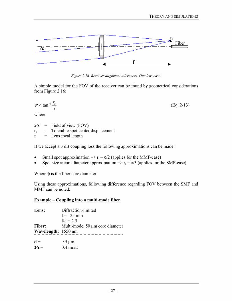
Figure 2.16. Receiver alignment tolerances. One lens case. A simple model for the FOV of the receiver can be found by geometrical considerations from Figure 2.16:
frs1tan −<α (Eq. 2-13)
where 2α = Field of view (FOV) rs = Tolerable spot center displacement f = Lens focal length If we accept a 3 dB coupling loss the following approximations can be made: • Small spot approximation => rs = φ/2 (applies for the MMF-case) • Spot size ≈ core diameter approximation => rs = φ/3 (applies for the SMF-case) Where φ is the fiber core diameter. Using these approximations, following difference regarding FOV between the SMF and MMF can be noted: Example – Coupling into a multi-mode fiber Lens: Diffraction-limited f = 125 mm f/# = 2.5 Fiber: Multi-mode, 50 µm core diameter Wavelength: 1550 nm d = 9.5 µm 2αααα = 0.4 mrad
αααα
rs Fiber
f
THEORY AND SIMULATIONS
- 28 -
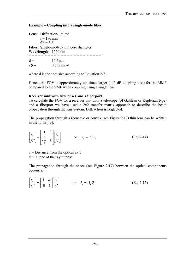
Example – Coupling into a single-mode fiber Lens: Diffraction-limited f = 190 mm f/# = 3.8 Fiber: Single-mode, 9 µm core diameter Wavelength: 1550 nm d = 14.4 µm 2αααα = 0.032 mrad where d is the spot size according to Equation 2-7. Hence, the FOV is approximately ten times larger (at 3 dB coupling loss) for the MMF compared to the SMF when coupling using a single lens. Receiver unit with two lenses and a fiberport To calculate the FOV for a receiver unit with a telescope (of Galilean or Keplerian type) and a fiberport we have used a 2x2 transfer matrix approach to describe the beam propagation through the lens system. Diffraction is neglected. The propagation through a (concave or convex, see Figure 2.17) thin lens can be written in the form [13].
or '1
f1-
0 1
' iloi
i
o
o r Ar rr
rr
=
=
(Eq. 2-14)
r = Distance from the optical axis r’ = Slope of the ray = tan α The propagation through the space (see Figure 2.17) between the optical components becomes:
or '10
1' iso
i
i
o
o r Ar rr
d
rr
=
=
(Eq. 2-15)
THEORY AND SIMULATIONS
- 29 -
Figure 2.17. Propagation through a thin lens and through space.
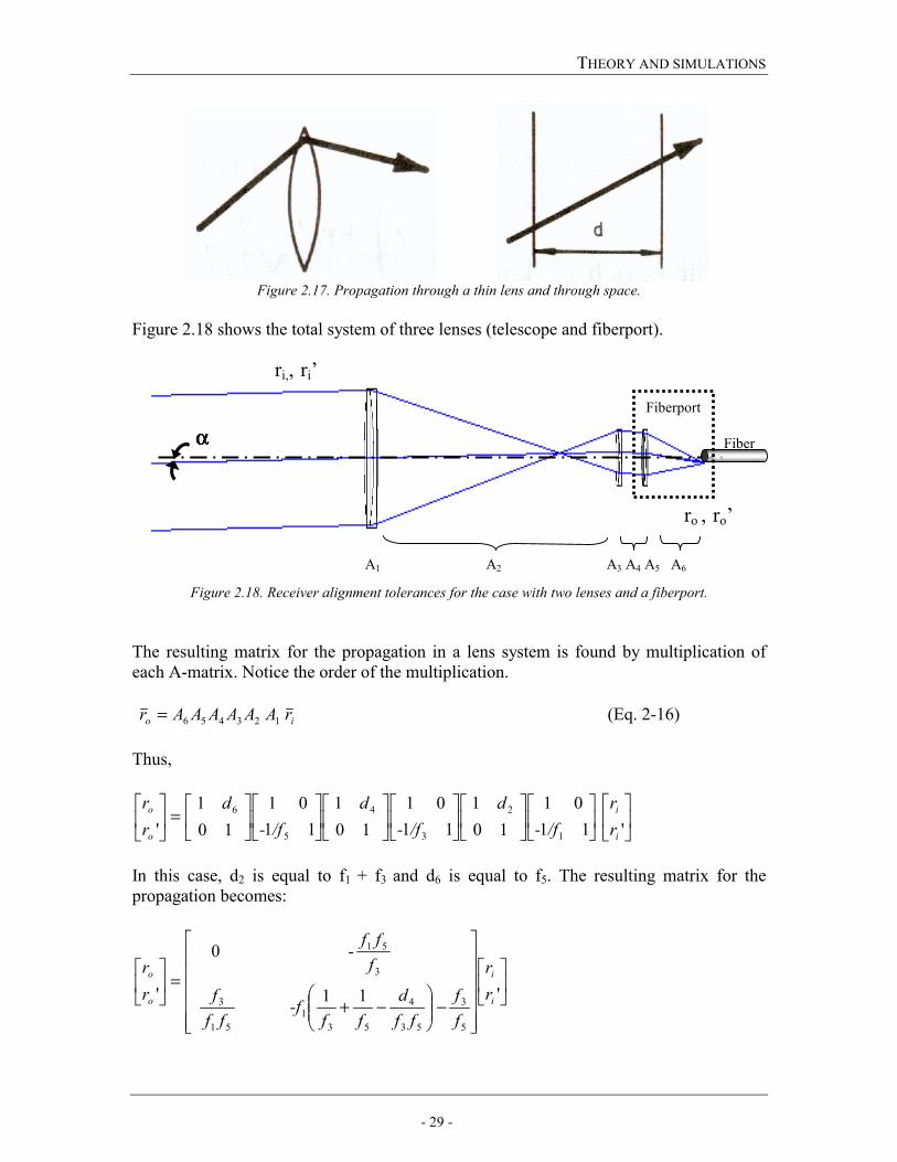
Figure 2.18 shows the total system of three lenses (telescope and fiberport).
Figure 2.18. Receiver alignment tolerances for the case with two lenses and a fiberport. The resulting matrix for the propagation in a lens system is found by multiplication of each A-matrix. Notice the order of the multiplication.
123456 io r AAAAAAr = (Eq. 2-16) Thus,
'11
0110
111
0110
111
0110
1' 1
2
3
4
5
6
=
i
i
o
o
rr
/f-
d /f-
d /f-
d rr
In this case, d2 is equal to f1 + f3 and d6 is equal to f5. The resulting matrix for the propagation becomes:
−
−+
=
'11
0
'
5
3
53
4
531
51
3
3
51
i
i
o
o
rr
ff
ffd
ff -f
fff
fff -
rr
Fiber
Fiberport
αααα
ri,, ri’
ro , ro’
A1 A2 A3 A4 A5 A6
THEORY AND SIMULATIONS
- 30 -
It is found that
αtan'3
51
3
51
fff
rfff
r io −=−= (Eq. 2-17)
Thus,
1
3
5
1tanff
frs−<α (Eq. 2-18)
This equation may be compared to the equation for the one-lens receiver case (Eq. 2-13),
to see the consequences of using a telescope and a fiberport instead of a one-lens receiver. Equation 2-18 may also be written in the form:
5
1
5
1
/#tantan
φα m
fr
rfm s
s−− =< (Eq. 2-19)
where m is the magnification factor and φ5 is the diameter of the incoming beam into the
fiberport lens. In both the one-lens and the telescope case, the optimal f/# is the same. The corresponding equation for the one-lens case would be:
φα 1
/#tantan 11
fr
fr ss −− =< (Eq. 2-20)
where φ is the diameter of the lens. In a comparison between these two equations, we see that there is no difference in the angle tolerances between using a (Keplerian or Galilean) telescope and using a one-lens receiver. This comes from the fact that φ5/m in Equation 2-19 is equal to φ in Equation 2-20.
THEORY AND SIMULATIONS
- 31 -
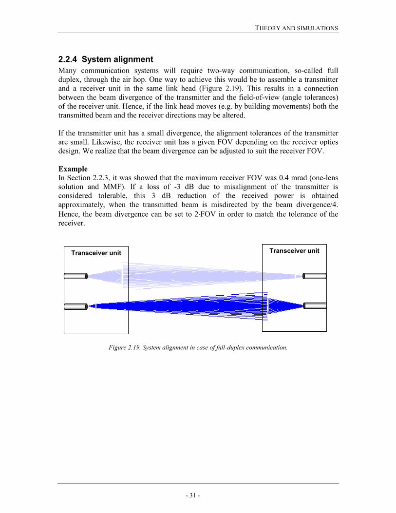
2.2.4 System alignment Many communication systems will require two-way communication, so-called full duplex, through the air hop. One way to achieve this would be to assemble a transmitter and a receiver unit in the same link head (Figure 2.19). This results in a connection between the beam divergence of the transmitter and the field-of-view (angle tolerances) of the receiver unit. Hence, if the link head moves (e.g. by building movements) both the transmitted beam and the receiver directions may be altered. If the transmitter unit has a small divergence, the alignment tolerances of the transmitter are small. Likewise, the receiver unit has a given FOV depending on the receiver optics design. We realize that the beam divergence can be adjusted to suit the receiver FOV.
Example In Section 2.2.3, it was showed that the maximum receiver FOV was 0.4 mrad (one-lens solution and MMF). If a loss of -3 dB due to misalignment of the transmitter is considered tolerable, this 3 dB reduction of the received power is obtained approximately, when the transmitted beam is misdirected by the beam divergence/4. Hence, the beam divergence can be set to 2⋅FOV in order to match the tolerance of the receiver.
Figure 2.19. System alignment in case of full-duplex communication.
Transceiver unitTransceiver unit
THEORY AND SIMULATIONS
- 32 -
2.3 Link budget
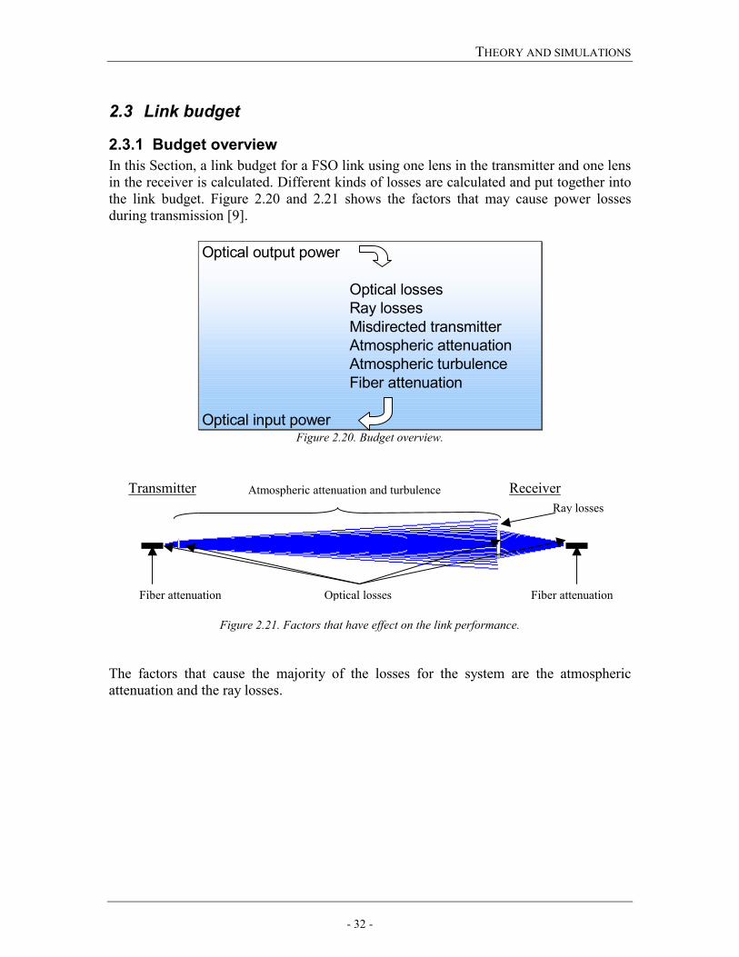
2.3.1 Budget overview In this Section, a link budget for a FSO link using one lens in the transmitter and one lens in the receiver is calculated. Different kinds of losses are calculated and put together into the link budget. Figure 2.20 and 2.21 shows the factors that may cause power losses during transmission [9].
Optical output power
Optical lossesRay lossesMisdirected transmitterAtmospheric attenuationAtmospheric turbulenceFiber attenuation
Optical input power Figure 2.20. Budget overview.
Figure 2.21. Factors that have effect on the link performance. The factors that cause the majority of the losses for the system are the atmospheric attenuation and the ray losses.
Transmitter Receiver
Fiber attenuation
Atmospheric attenuation and turbulence Ray losses
Optical losses Fiber attenuation
THEORY AND SIMULATIONS
- 33 -
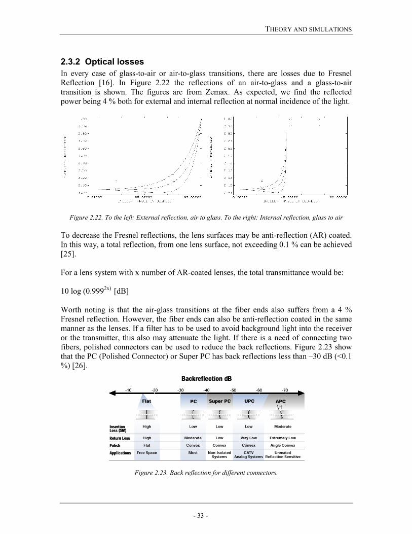
2.3.2 Optical losses In every case of glass-to-air or air-to-glass transitions, there are losses due to Fresnel Reflection [16]. In Figure 2.22 the reflections of an air-to-glass and a glass-to-air transition is shown. The figures are from Zemax. As expected, we find the reflected power being 4 % both for external and internal reflection at normal incidence of the light.
Figure 2.22. To the left: External reflection, air to glass. To the right: Internal reflection, glass to air To decrease the Fresnel reflections, the lens surfaces may be anti-reflection (AR) coated. In this way, a total reflection, from one lens surface, not exceeding 0.1 % can be achieved [25]. For a lens system with x number of AR-coated lenses, the total transmittance would be: 10 log (0.9992x) [dB] Worth noting is that the air-glass transitions at the fiber ends also suffers from a 4 % Fresnel reflection. However, the fiber ends can also be anti-reflection coated in the same manner as the lenses. If a filter has to be used to avoid background light into the receiver or the transmitter, this also may attenuate the light. If there is a need of connecting two fibers, polished connectors can be used to reduce the back reflections. Figure 2.23 show that the PC (Polished Connector) or Super PC has back reflections less than –30 dB (<0.1 %) [26].
Figure 2.23. Back reflection for different connectors.
THEORY AND SIMULATIONS
- 34 -
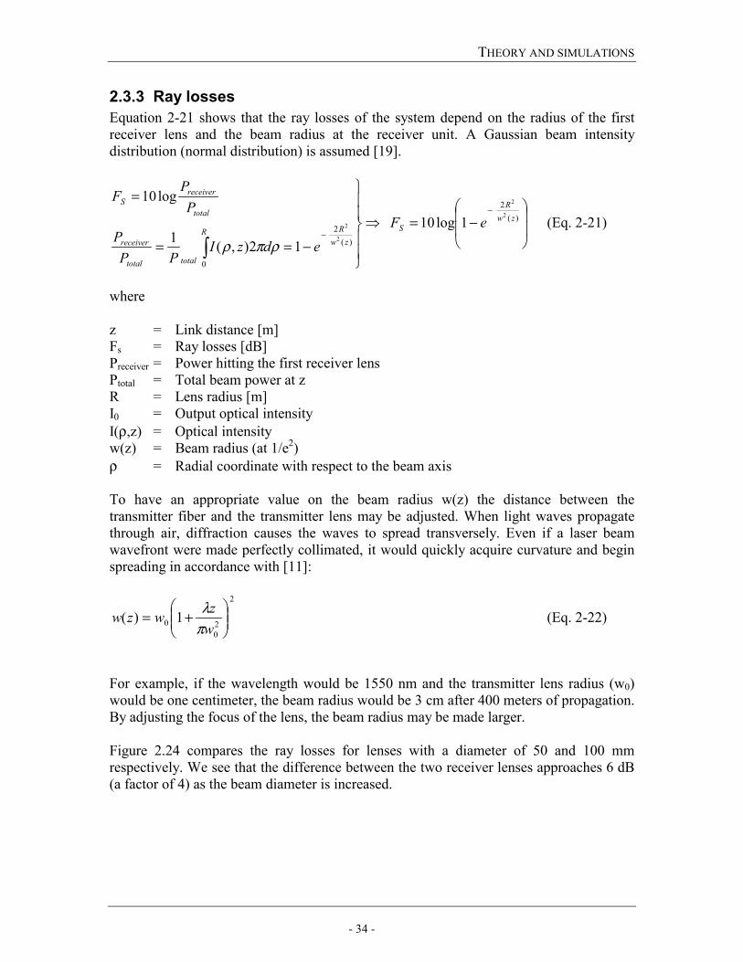
2.3.3 Ray losses Equation 2-21 shows that the ray losses of the system depend on the radius of the first receiver lens and the beam radius at the receiver unit. A Gaussian beam intensity distribution (normal distribution) is assumed [19].
−=
−==
=−
−
)(2
)(2
0
2
2
2
2 1log10
12),(1
log10zw
R
Szw
RR
totaltotal
receiver
total
receiverS
eFedzI
PPP
PP
F
ρπρ (Eq. 2-21)
where z = Link distance [m] Fs = Ray losses [dB] Preceiver = Power hitting the first receiver lens Ptotal = Total beam power at z R = Lens radius [m] I0 = Output optical intensity I(ρ,z) = Optical intensity w(z) = Beam radius (at 1/e2) ρ = Radial coordinate with respect to the beam axis To have an appropriate value on the beam radius w(z) the distance between the transmitter fiber and the transmitter lens may be adjusted. When light waves propagate through air, diffraction causes the waves to spread transversely. Even if a laser beam wavefront were made perfectly collimated, it would quickly acquire curvature and begin spreading in accordance with [11]:
2
20
0 1)(
+=
wzwzw
πλ (Eq. 2-22)
For example, if the wavelength would be 1550 nm and the transmitter lens radius (w0) would be one centimeter, the beam radius would be 3 cm after 400 meters of propagation. By adjusting the focus of the lens, the beam radius may be made larger. Figure 2.24 compares the ray losses for lenses with a diameter of 50 and 100 mm respectively. We see that the difference between the two receiver lenses approaches 6 dB (a factor of 4) as the beam diameter is increased.
THEORY AND SIMULATIONS
- 35 -
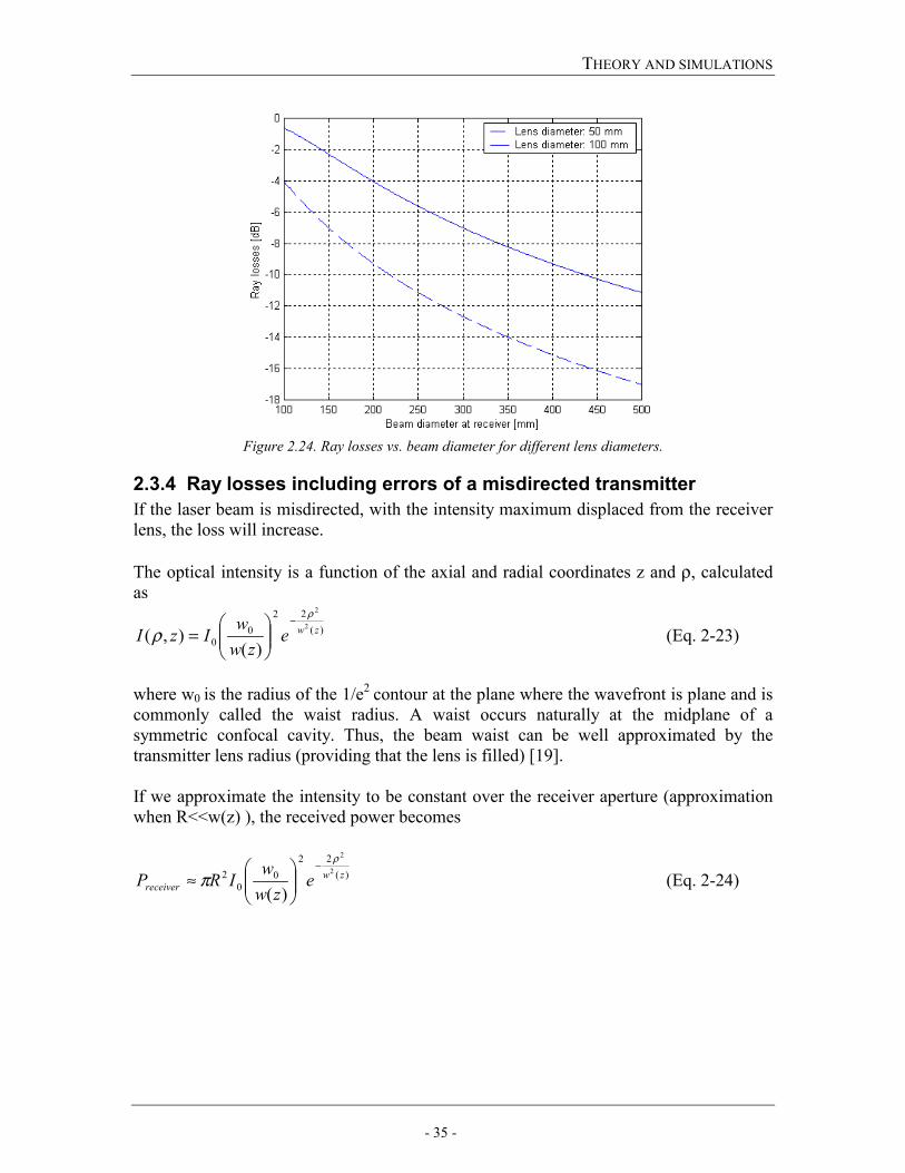
Figure 2.24. Ray losses vs. beam diameter for different lens diameters.
2.3.4 Ray losses including errors of a misdirected transmitter If the laser beam is misdirected, with the intensity maximum displaced from the receiver lens, the loss will increase. The optical intensity is a function of the axial and radial coordinates z and ρ, calculated as
)(22
00
2
2
)(),( zwe
zww
IzIρ
ρ−
= (Eq. 2-23)
where w0 is the radius of the 1/e2 contour at the plane where the wavefront is plane and is commonly called the waist radius. A waist occurs naturally at the midplane of a symmetric confocal cavity. Thus, the beam waist can be well approximated by the transmitter lens radius (providing that the lens is filled) [19]. If we approximate the intensity to be constant over the receiver aperture (approximation when R<<w(z) ), the received power becomes
)(22
00
2 2
2
)(zw
receiver ezw
wIRP
ρ
π−
≈ (Eq. 2-24)
THEORY AND SIMULATIONS
- 36 -
Since the total beam power is given by 200
0 212),( wIdzIPtotal πρπρ ==
∞
(Eq. 2-25)
the ratio of the power carried within the receiver aperture to the total power becomes
)(2
21
)(2
)(2
2
200
)(22
00
22
22
2
zweR
wI
ezw
wIR
PP zw
zw
total
receiver
ρρ
π
π −−
=
= (Eq. 2-26)
Thus
=−
)(2log10 2
)(2
2 2
2
zweRF
zw
S
ρ
(Eq. 2-27)
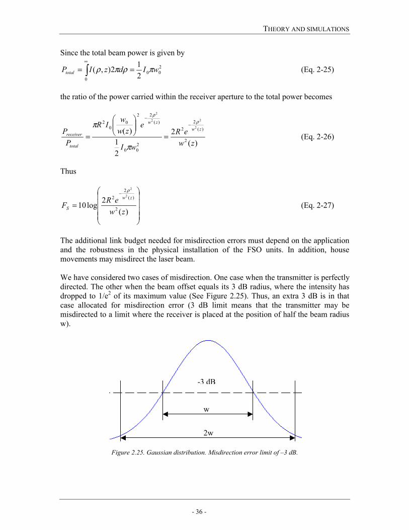
The additional link budget needed for misdirection errors must depend on the application and the robustness in the physical installation of the FSO units. In addition, house movements may misdirect the laser beam. We have considered two cases of misdirection. One case when the transmitter is perfectly directed. The other when the beam offset equals its 3 dB radius, where the intensity has dropped to 1/e2 of its maximum value (See Figure 2.25). Thus, an extra 3 dB is in that case allocated for misdirection error (3 dB limit means that the transmitter may be misdirected to a limit where the receiver is placed at the position of half the beam radius w).
Figure 2.25. Gaussian distribution. Misdirection error limit of –3 dB.
w
2w
-3 dB
THEORY AND SIMULATIONS
- 37 -
2.3.5 Atmospheric attenuation When the laser beam propagates through the air, it is exposed to attenuation depending on the weather conditions. The equation of the laser transmission in air is described by Beer’s law as [7,9]:
( )zL
z
total
receiver eFeP
Pz σστ −− === log10)( (Eq. 2-28)
where τ = Transmission FL = Attenuation [dB] Preceiver = Received power Ptotal = Transmitted power σ = Atmosphere attenuation or total extinction coefficient z = Distance between transmitter and receiver in kilometers The total extinction coefficient σ can be divided into four parts:
amam ββαασ +++= where αm = Molecular absorption coefficient αa = Aerosol absorption coefficient βm = Molecular or Rayleigh scattering coefficient βa = Aerosol or Mie scattering coefficient. It is common to choose a laser wavelength that makes the gas absorption and molecule scattering negligible. For wavelengths between the visual band and 1.5 µm the molecular absorption, aerosol absorption and the molecular scattering are small compared with the aerosol scattering, which dominates the total extinction coefficient [9].
THEORY AND SIMULATIONS
- 38 -
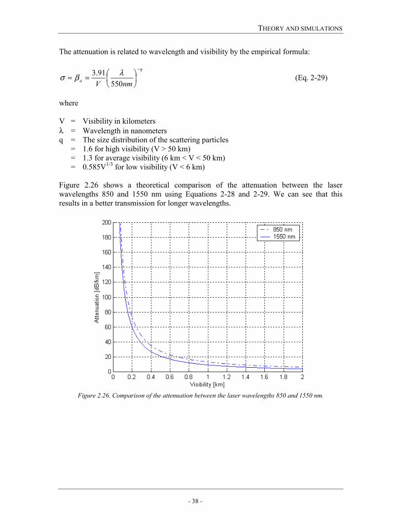
The attenuation is related to wavelength and visibility by the empirical formula:
q
a nmV
−
=≈550
91.3 λβσ (Eq. 2-29)
where V = Visibility in kilometers λ = Wavelength in nanometers q = The size distribution of the scattering particles = 1.6 for high visibility (V > 50 km) = 1.3 for average visibility (6 km < V < 50 km) = 0.585V1/3 for low visibility (V < 6 km) Figure 2.26 shows a theoretical comparison of the attenuation between the laser wavelengths 850 and 1550 nm using Equations 2-28 and 2-29. We can see that this results in a better transmission for longer wavelengths.
Figure 2.26. Comparison of the attenuation between the laser wavelengths 850 and 1550 nm.
THEORY AND SIMULATIONS
- 39 -
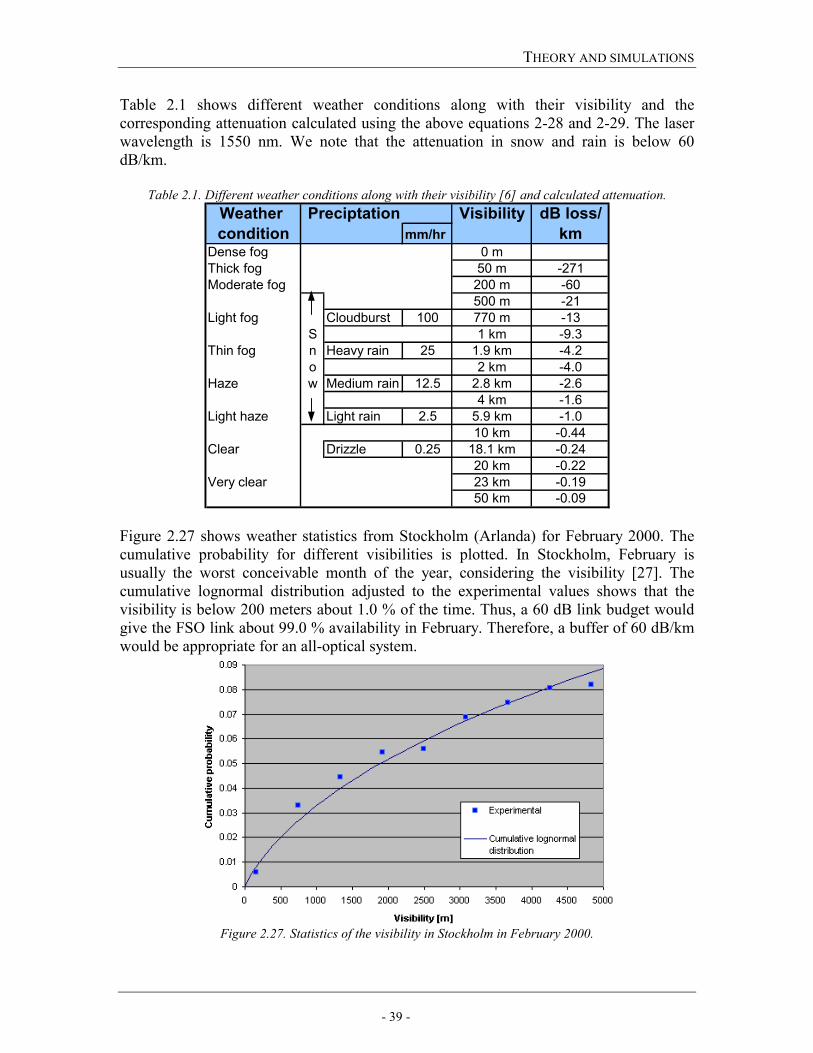
Table 2.1 shows different weather conditions along with their visibility and the corresponding attenuation calculated using the above equations 2-28 and 2-29. The laser wavelength is 1550 nm. We note that the attenuation in snow and rain is below 60 dB/km.
Table 2.1. Different weather conditions along with their visibility [6] and calculated attenuation. Weather Preciptation Visibility dB loss/condition mm/hr km
Dense fog 0 mThick fog 50 m -271Moderate fog 200 m -60
500 m -21Light fog Cloudburst 100 770 m -13
S 1 km -9.3Thin fog n Heavy rain 25 1.9 km -4.2
o 2 km -4.0Haze w Medium rain 12.5 2.8 km -2.6
4 km -1.6Light haze Light rain 2.5 5.9 km -1.0
10 km -0.44Clear Drizzle 0.25 18.1 km -0.24
20 km -0.22Very clear 23 km -0.19
50 km -0.09 Figure 2.27 shows weather statistics from Stockholm (Arlanda) for February 2000. The cumulative probability for different visibilities is plotted. In Stockholm, February is usually the worst conceivable month of the year, considering the visibility [27]. The cumulative lognormal distribution adjusted to the experimental values shows that the visibility is below 200 meters about 1.0 % of the time. Thus, a 60 dB link budget would give the FSO link about 99.0 % availability in February. Therefore, a buffer of 60 dB/km would be appropriate for an all-optical system.
Figure 2.27. Statistics of the visibility in Stockholm in February 2000.
THEORY AND SIMULATIONS
- 40 -
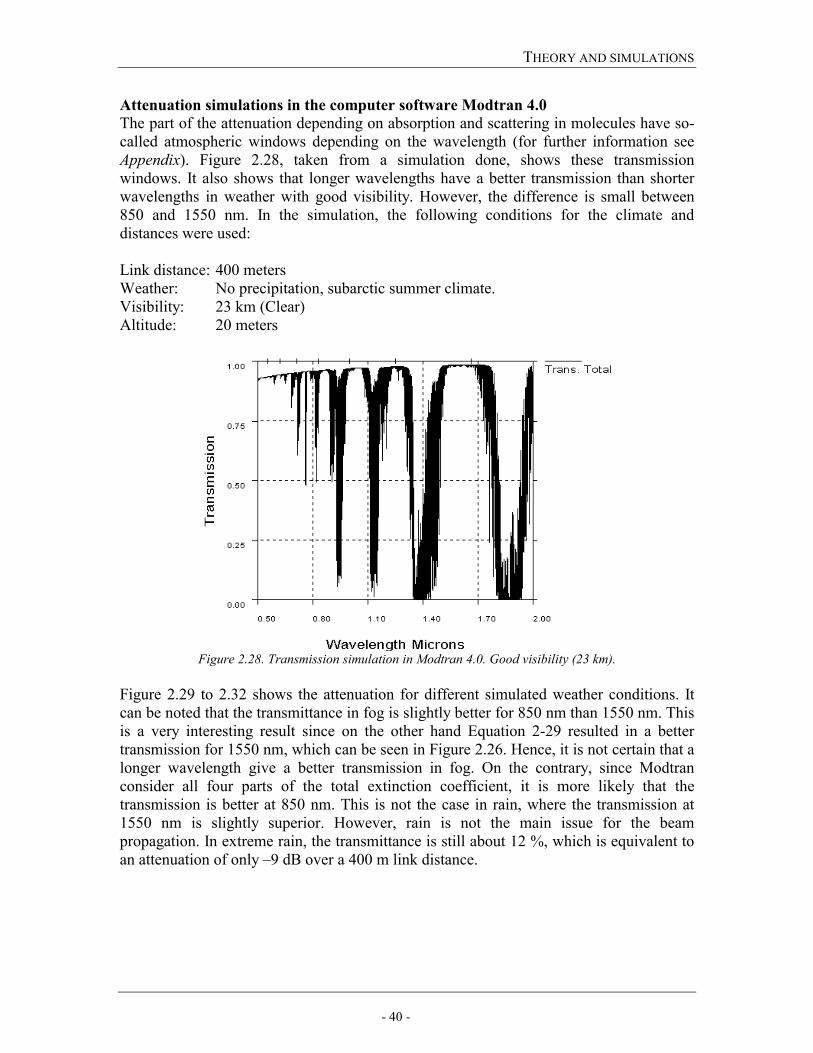
Attenuation simulations in the computer software Modtran 4.0 The part of the attenuation depending on absorption and scattering in molecules have so-called atmospheric windows depending on the wavelength (for further information see Appendix). Figure 2.28, taken from a simulation done, shows these transmission windows. It also shows that longer wavelengths have a better transmission than shorter wavelengths in weather with good visibility. However, the difference is small between 850 and 1550 nm. In the simulation, the following conditions for the climate and distances were used: Link distance: 400 meters Weather: No precipitation, subarctic summer climate. Visibility: 23 km (Clear) Altitude: 20 meters
Figure 2.28. Transmission simulation in Modtran 4.0. Good visibility (23 km).
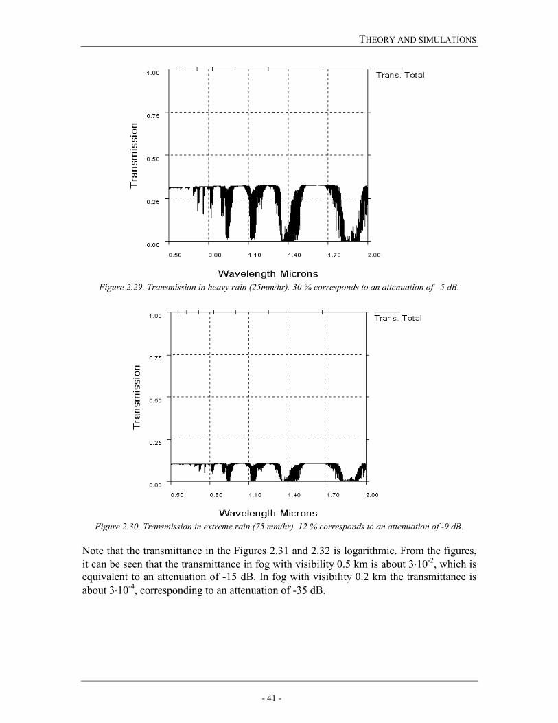
Figure 2.29 to 2.32 shows the attenuation for different simulated weather conditions. It can be noted that the transmittance in fog is slightly better for 850 nm than 1550 nm. This is a very interesting result since on the other hand Equation 2-29 resulted in a better transmission for 1550 nm, which can be seen in Figure 2.26. Hence, it is not certain that a longer wavelength give a better transmission in fog. On the contrary, since Modtran consider all four parts of the total extinction coefficient, it is more likely that the transmission is better at 850 nm. This is not the case in rain, where the transmission at 1550 nm is slightly superior. However, rain is not the main issue for the beam propagation. In extreme rain, the transmittance is still about 12 %, which is equivalent to an attenuation of only –9 dB over a 400 m link distance.
THEORY AND SIMULATIONS
- 41 -
Figure 2.29. Transmission in heavy rain (25mm/hr). 30 % corresponds to an attenuation of –5 dB.
Figure 2.30. Transmission in extreme rain (75 mm/hr). 12 % corresponds to an attenuation of -9 dB.
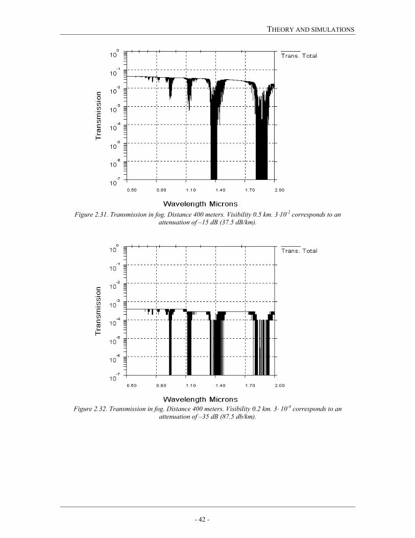
Note that the transmittance in the Figures 2.31 and 2.32 is logarithmic. From the figures, it can be seen that the transmittance in fog with visibility 0.5 km is about 3⋅10-2, which is equivalent to an attenuation of -15 dB. In fog with visibility 0.2 km the transmittance is about 3⋅10-4, corresponding to an attenuation of -35 dB.
THEORY AND SIMULATIONS
- 42 -
Figure 2.31. Transmission in fog. Distance 400 meters. Visibility 0.5 km. 3⋅10-2 corresponds to an
attenuation of –15 dB (37.5 dB/km).
Figure 2.32. Transmission in fog. Distance 400 meters. Visibility 0.2 km. 3⋅ 10-4 corresponds to an
attenuation of –35 dB (87.5 db/km).
THEORY AND SIMULATIONS
- 43 -
2.3.6 Atmospheric turbulence Scintillations and beam wandering
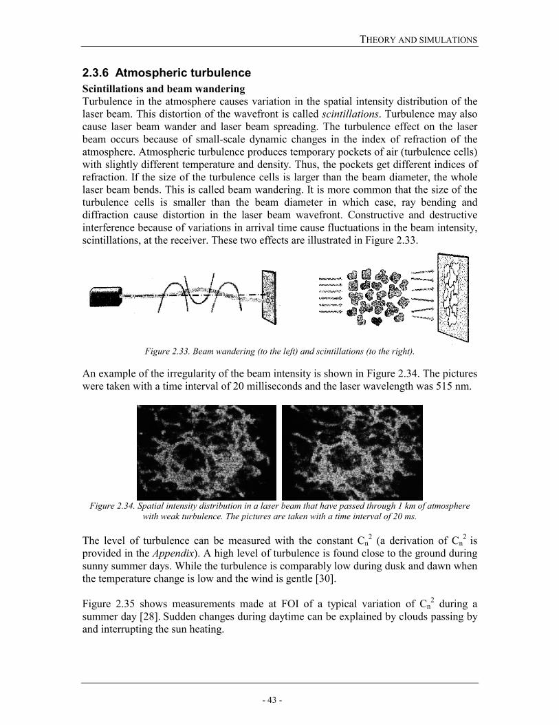
Turbulence in the atmosphere causes variation in the spatial intensity distribution of the laser beam. This distortion of the wavefront is called scintillations. Turbulence may also cause laser beam wander and laser beam spreading. The turbulence effect on the laser beam occurs because of small-scale dynamic changes in the index of refraction of the atmosphere. Atmospheric turbulence produces temporary pockets of air (turbulence cells) with slightly different temperature and density. Thus, the pockets get different indices of refraction. If the size of the turbulence cells is larger than the beam diameter, the whole laser beam bends. This is called beam wandering. It is more common that the size of the turbulence cells is smaller than the beam diameter in which case, ray bending and diffraction cause distortion in the laser beam wavefront. Constructive and destructive interference because of variations in arrival time cause fluctuations in the beam intensity, scintillations, at the receiver. These two effects are illustrated in Figure 2.33.
Figure 2.33. Beam wandering (to the left) and scintillations (to the right).
An example of the irregularity of the beam intensity is shown in Figure 2.34. The pictures were taken with a time interval of 20 milliseconds and the laser wavelength was 515 nm.
Figure 2.34. Spatial intensity distribution in a laser beam that have passed through 1 km of atmosphere
with weak turbulence. The pictures are taken with a time interval of 20 ms. The level of turbulence can be measured with the constant Cn
2 (a derivation of Cn2 is
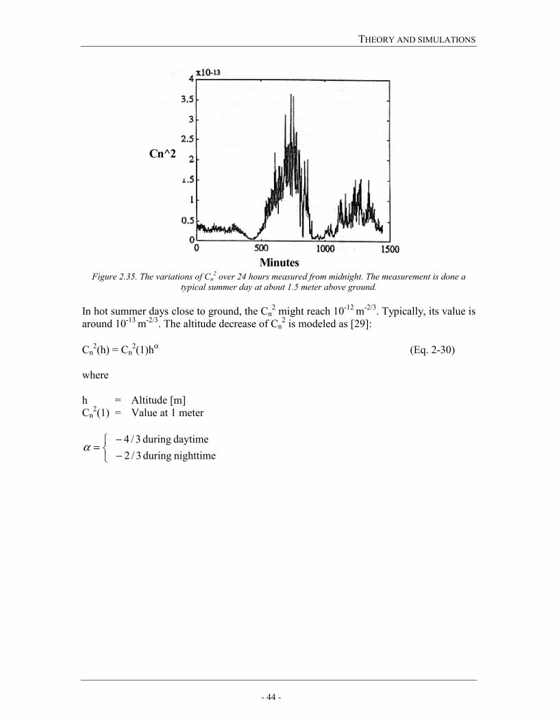
provided in the Appendix). A high level of turbulence is found close to the ground during sunny summer days. While the turbulence is comparably low during dusk and dawn when the temperature change is low and the wind is gentle [30]. Figure 2.35 shows measurements made at FOI of a typical variation of Cn
2 during a summer day [28]. Sudden changes during daytime can be explained by clouds passing by and interrupting the sun heating.
THEORY AND SIMULATIONS
- 44 -
Minutes
Cn^2
Figure 2.35. The variations of Cn
2 over 24 hours measured from midnight. The measurement is done a typical summer day at about 1.5 meter above ground.
In hot summer days close to ground, the Cn
2 might reach 10-12 m-2/3. Typically, its value is around 10-13 m-2/3. The altitude decrease of Cn
2 is modeled as [29]: Cn
2(h) = Cn2(1)hα (Eq. 2-30)
where h = Altitude [m] Cn
2(1) = Value at 1 meter
−−
=nighttime during 3/2 daytime during 3/4
α
THEORY AND SIMULATIONS
- 45 -
Probability of fading If the scintillations due to turbulence are strong, they may cause so-called fading. Fading occurs when the signal power diminishes below a certain threshold value. This may give rise to bit errors (in our case the error ‘1’ detected as ‘0’). The probability that the irradiance (I) falls below the threshold value IT is [9,30]:
++
+=≤),(2
),0(ln2),(
21
121)(
2
22
z
zII
wz
erfIIpI
T
eI
T ρσ
ρρσ (Eq. 2-31)
where σI
2 = Normalized irradiance variance ρ = Radial coordinate with respect to the beam axis (ρ = 0 at the beam axis) we = Beam radius after turbulence influence z = Link distance erf(X) is the error function for each element of X, where X must be real. The error function is defined as:
( )dteXerfX
t
−=0
22)(π
and where a relative threshold can be defined as:
=
TT I
zIF
),0(log10 [dB] (Eq. 2-32)
See appendix for more details about irradiance variance. Figure 2.36 shows the probability of fading as a function of the threshold FT. The following constants have been used in a computer: z = 400 meter we = 0.1 meter ρ = 0 λ = 1550 nm The model does also take into account the size of the receiver aperture and its averaging effect (Eq. 6-5 in Appendix). The lens diameter in this example was set to 50 mm.
THEORY AND SIMULATIONS
- 46 -
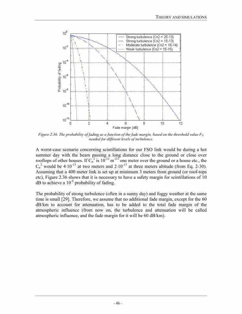
Figure 2.36. The probability of fading as a function of the fade margin, based on the threshold value FT,
needed for different levels of turbulence. A worst-case scenario concerning scintillations for our FSO link would be during a hot summer day with the beam passing a long distance close to the ground or close over rooftops of other houses. If Cn
2 is 10-12 m-2/3 one meter over the ground or a house etc., the
Cn2 would be 4⋅10-13 at two meters and 2⋅10-13 at three meters altitude (from Eq. 2-30).
Assuming that a 400 meter link is set up at minimum 3 meters from ground (or roof-tops etc), Figure 2.36 shows that it is necessary to have a safety margin for scintillations of 10 dB to achieve a 10-9 probability of fading. The probability of strong turbulence (often in a sunny day) and foggy weather at the same time is small [29]. Therefore, we assume that no additional fade margin, except for the 60 dB/km to account for attenuation, has to be added to the total fade margin of the atmospheric influence (from now on, the turbulence and attenuation will be called atmospheric influence, and the fade margin for it will be 60 dB/km).
THEORY AND SIMULATIONS
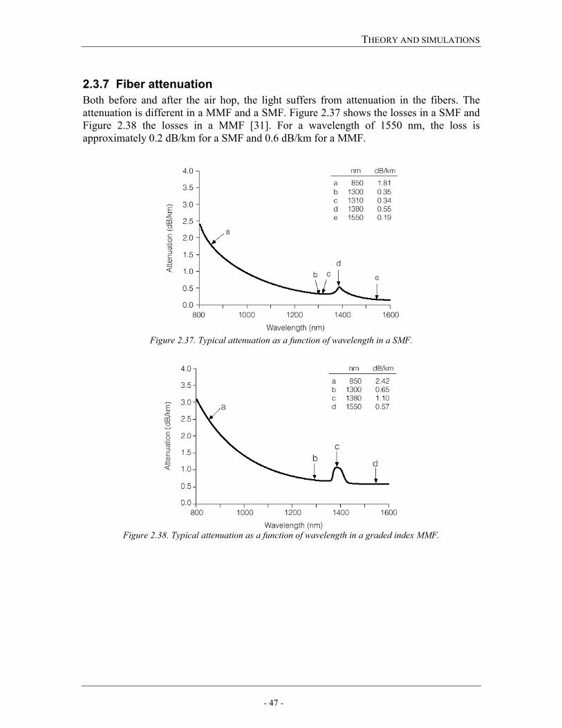
- 47 -
2.3.7 Fiber attenuation Both before and after the air hop, the light suffers from attenuation in the fibers. The attenuation is different in a MMF and a SMF. Figure 2.37 shows the losses in a SMF and Figure 2.38 the losses in a MMF [31]. For a wavelength of 1550 nm, the loss is approximately 0.2 dB/km for a SMF and 0.6 dB/km for a MMF.
Figure 2.37. Typical attenuation as a function of wavelength in a SMF.
Figure 2.38. Typical attenuation as a function of wavelength in a graded index MMF.
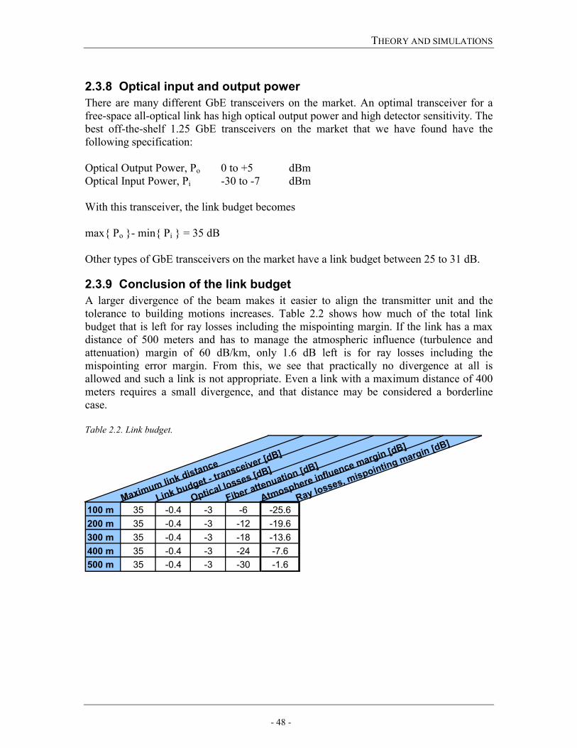
THEORY AND SIMULATIONS
- 48 -
2.3.8 Optical input and output power There are many different GbE transceivers on the market. An optimal transceiver for a free-space all-optical link has high optical output power and high detector sensitivity. The best off-the-shelf 1.25 GbE transceivers on the market that we have found have the following specification: Optical Output Power, Po 0 to +5 dBm Optical Input Power, Pi -30 to -7 dBm With this transceiver, the link budget becomes max Po - min Pi = 35 dB Other types of GbE transceivers on the market have a link budget between 25 to 31 dB.
2.3.9 Conclusion of the link budget A larger divergence of the beam makes it easier to align the transmitter unit and the tolerance to building motions increases. Table 2.2 shows how much of the total link budget that is left for ray losses including the mispointing margin. If the link has a max distance of 500 meters and has to manage the atmospheric influence (turbulence and attenuation) margin of 60 dB/km, only 1.6 dB left is for ray losses including the mispointing error margin. From this, we see that practically no divergence at all is allowed and such a link is not appropriate. Even a link with a maximum distance of 400 meters requires a small divergence, and that distance may be considered a borderline case. Table 2.2. Link budget.
Maximum link distance
Link budget - transceiver [dB]
Optical losses [dB]
Fiber attenuation [dB]
Atmosphere influence margin [dB]
Ray losses, mispointing margin [dB]
100 m 35 -0.4 -3 -6 -25.6200 m 35 -0.4 -3 -12 -19.6300 m 35 -0.4 -3 -18 -13.6400 m 35 -0.4 -3 -24 -7.6500 m 35 -0.4 -3 -30 -1.6
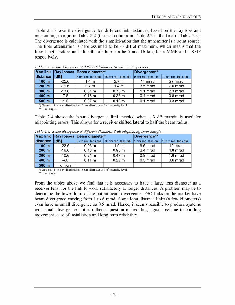
THEORY AND SIMULATIONS
- 49 -
Table 2.3 shows the divergence for different link distances, based on the ray loss and mispointing margin in Table 2.2 (the last column in Table 2.2 is the first in Table 2.3). The divergence is calculated with the simplification that the transmitter is a point source. The fiber attenuation is here assumed to be -3 dB at maximum, which means that the fiber length before and after the air hop can be 5 and 16 km, for a MMF and a SMF respectively. Table 2.3. Beam divergence at different distances. No mispointing errors. Max link Ray losses Beam diameter* Divergence**distance [dB] 5 cm rec. lens dia. 10 cm rec. lens dia. 5 cm rec. lens dia. 10 cm rec. lens dia.
100 m -25.6 1.4 m 2.7 m 14 mrad 27 mrad200 m -19.6 0.7 m 1.4 m 3.5 mrad 7.0 mrad300 m -13.6 0.34 m 0.70 m 1.1 mrad 2.3 mrad400 m -7.6 0.16 m 0.33 m 0.4 mrad 0.8 mrad500 m -1.6 0.07 m 0.13 m 0.1 mrad 0.3 mrad
*) Gaussian intensity distribution. Beam diameter at 1/e2 intensity level. **) Full angle. Table 2.4 shows the beam divergence limit needed when a 3 dB margin is used for mispointing errors. This allows for a receiver shifted lateral to half the beam radius. Table 2.4. Beam divergence at different distances. 3 dB mispointing error margin. Max link Ray losses Beam diameter* Divergence**distance [dB] 5 cm rec. lens dia. 10 cm rec. lens dia. 5 cm rec. lens dia. 10 cm rec. lens dia.
100 m -22.6 0.96 m 1.9 m 9.6 mrad 19 mrad200 m -16.6 0.48 m 0.96 m 2.4 mrad 4.8 mrad300 m -10.6 0.24 m 0.47 m 0.8 mrad 1.6 mrad400 m -4.6 0.11 m 0.22 m 0.3 mrad 0.6 mrad500 m to high
*) Gaussian intensity distribution. Beam diameter at 1/e2 intensity level. **) Full angle. From the tables above we find that it is necessary to have a large lens diameter as a receiver lens, for the link to work satisfactory at longer distances. A problem may be to determine the lower limit of the output beam divergence. FSO links on the market have beam divergence varying from 1 to 6 mrad. Some long distance links (a few kilometers) even have as small divergence as 0.5 mrad. Hence, it seems possible to produce systems with small divergence – it is rather a question of avoiding signal loss due to building movement, ease of installation and long-term reliability.
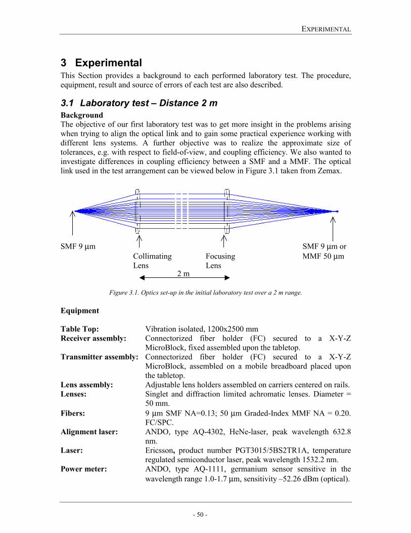
EXPERIMENTAL
- 50 -
3 Experimental This Section provides a background to each performed laboratory test. The procedure, equipment, result and source of errors of each test are also described.
3.1 Laboratory test – Distance 2 m Background
The objective of our first laboratory test was to get more insight in the problems arising when trying to align the optical link and to gain some practical experience working with different lens systems. A further objective was to realize the approximate size of tolerances, e.g. with respect to field-of-view, and coupling efficiency. We also wanted to investigate differences in coupling efficiency between a SMF and a MMF. The optical link used in the test arrangement can be viewed below in Figure 3.1 taken from Zemax.
SMF 9 µm SMF 9 µm or Collimating Focusing MMF 50 µm Lens Lens
Figure 3.1. Optics set-up in the initial laboratory test over a 2 m range.
Equipment Table Top: Vibration isolated, 1200x2500 mm Receiver assembly: Connectorized fiber holder (FC) secured to a X-Y-Z
MicroBlock, fixed assembled upon the tabletop. Transmitter assembly: Connectorized fiber holder (FC) secured to a X-Y-Z
MicroBlock, assembled on a mobile breadboard placed upon the tabletop.
Lens assembly: Adjustable lens holders assembled on carriers centered on rails. Lenses: Singlet and diffraction limited achromatic lenses. Diameter =
50 mm. Fibers: 9 µm SMF NA=0.13; 50 µm Graded-Index MMF NA = 0.20.
FC/SPC. Alignment laser: ANDO, type AQ-4302, HeNe-laser, peak wavelength 632.8
nm. Laser: Ericsson, product number PGT3015/5BS2TR1A, temperature
regulated semiconductor laser, peak wavelength 1532.2 nm. Power meter: ANDO, type AQ-1111, germanium sensor sensitive in the
wavelength range 1.0-1.7 µm, sensitivity –52.26 dBm (optical).
2 m
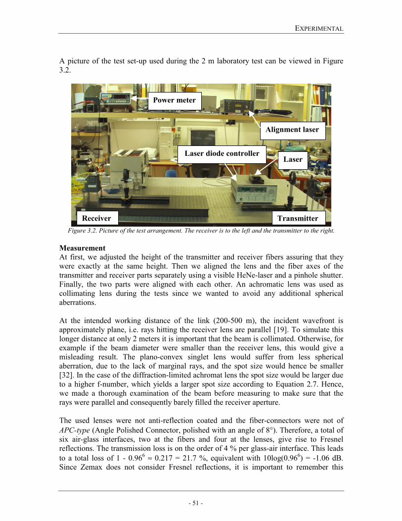
EXPERIMENTAL
- 51 -
A picture of the test set-up used during the 2 m laboratory test can be viewed in Figure 3.2.
Figure 3.2. Picture of the test arrangement. The receiver is to the left and the transmitter to the right.
Measurement
At first, we adjusted the height of the transmitter and receiver fibers assuring that they were exactly at the same height. Then we aligned the lens and the fiber axes of the transmitter and receiver parts separately using a visible HeNe-laser and a pinhole shutter. Finally, the two parts were aligned with each other. An achromatic lens was used as collimating lens during the tests since we wanted to avoid any additional spherical aberrations. At the intended working distance of the link (200-500 m), the incident wavefront is approximately plane, i.e. rays hitting the receiver lens are parallel [19]. To simulate this longer distance at only 2 meters it is important that the beam is collimated. Otherwise, for example if the beam diameter were smaller than the receiver lens, this would give a misleading result. The plano-convex singlet lens would suffer from less spherical aberration, due to the lack of marginal rays, and the spot size would hence be smaller [32]. In the case of the diffraction-limited achromat lens the spot size would be larger due to a higher f-number, which yields a larger spot size according to Equation 2.7. Hence, we made a thorough examination of the beam before measuring to make sure that the rays were parallel and consequently barely filled the receiver aperture. The used lenses were not anti-reflection coated and the fiber-connectors were not of APC-type (Angle Polished Connector, polished with an angle of 8°). Therefore, a total of six air-glass interfaces, two at the fibers and four at the lenses, give rise to Fresnel reflections. The transmission loss is on the order of 4 % per glass-air interface. This leads to a total loss of 1 - 0.966 ≈ 0.217 = 21.7 %, equivalent with 10log(0.966) = -1.06 dB. Since Zemax does not consider Fresnel reflections, it is important to remember this
Alignment laser
Power meter
Laser Laser diode controller
Receiver Transmitter
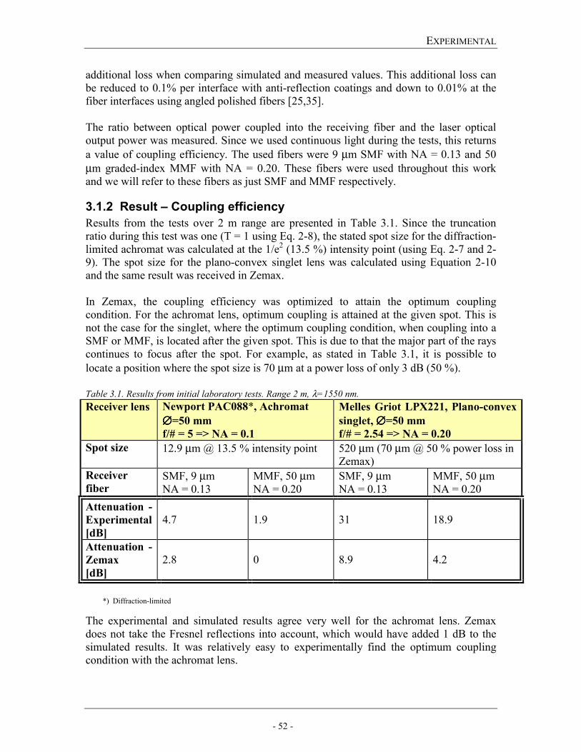
EXPERIMENTAL
- 52 -
additional loss when comparing simulated and measured values. This additional loss can be reduced to 0.1% per interface with anti-reflection coatings and down to 0.01% at the fiber interfaces using angled polished fibers [25,35]. The ratio between optical power coupled into the receiving fiber and the laser optical output power was measured. Since we used continuous light during the tests, this returns a value of coupling efficiency. The used fibers were 9 µm SMF with NA = 0.13 and 50 µm graded-index MMF with NA = 0.20. These fibers were used throughout this work and we will refer to these fibers as just SMF and MMF respectively.
3.1.2 Result – Coupling efficiency Results from the tests over 2 m range are presented in Table 3.1. Since the truncation ratio during this test was one (T = 1 using Eq. 2-8), the stated spot size for the diffraction-limited achromat was calculated at the 1/e2 (13.5 %) intensity point (using Eq. 2-7 and 2-9). The spot size for the plano-convex singlet lens was calculated using Equation 2-10 and the same result was received in Zemax. In Zemax, the coupling efficiency was optimized to attain the optimum coupling condition. For the achromat lens, optimum coupling is attained at the given spot. This is not the case for the singlet, where the optimum coupling condition, when coupling into a SMF or MMF, is located after the given spot. This is due to that the major part of the rays continues to focus after the spot. For example, as stated in Table 3.1, it is possible to locate a position where the spot size is 70 µm at a power loss of only 3 dB (50 %). Table 3.1. Results from initial laboratory tests. Range 2 m, λ=1550 nm. Receiver lens Newport PAC088*, Achromat
∅∅∅∅=50 mm f/# = 5 => NA = 0.1
Melles Griot LPX221, Plano-convex singlet, ∅∅∅∅=50 mm f/# = 2.54 => NA = 0.20
Spot size
12.9 µm @ 13.5 % intensity point 520 µm (70 µm @ 50 % power loss in Zemax)
Receiver fiber
SMF, 9 µm NA = 0.13
MMF, 50 µm NA = 0.20
SMF, 9 µm NA = 0.13
MMF, 50 µm NA = 0.20
Attenuation -Experimental [dB]
4.7
1.9
31
18.9
Attenuation - Zemax [dB]
2.8
0
8.9
4.2
*) Diffraction-limited
The experimental and simulated results agree very well for the achromat lens. Zemax does not take the Fresnel reflections into account, which would have added 1 dB to the simulated results. It was relatively easy to experimentally find the optimum coupling condition with the achromat lens.
EXPERIMENTAL
- 53 -
On the other hand, with the singlet lens, the results are not in good agreement. Apart from the Fresnel reflections, this is because it was very difficult to experimentally achieve the optimum coupling condition received in Zemax.
Source of errors During these tests, we did not know how to calculate coupling efficiency using Zemax. In the singlet-case, this probably made us stop seeking after the maximum too soon, during the experimental test, believing that we had found the global maximum, when we had actually found a local maximum. The singlet produces a much larger spot size, which makes it more difficult to find the maximum. The presented values of coupling efficiency from Zemax are calculated afterwards. The singlet lens had an f-number of 2.5, which yields NA = 0.20. This is above the NA of the SM-fiber, which means that part of the incoming light will have an angle that exceeds the angle of acceptance of the fiber.
3.2 Laboratory test – Distance 180 m Background
These tests were performed in a 100 m long laboratory. The transmitter and receiver units were placed side by side in one end of the laboratory. The optical path of 180 m was achieved by reflecting the beam using a flat mirror at the distance of 90 m. The purpose of these tests was to select, one of the different conceivable designs developed using calculations and Zemax, for the receiver unit. We evaluated the different designs by measuring coupling efficiency and FOV. We also wanted to get an understanding of other possible differences between the designs, e.g. with respect to alignment problems.
Equipment
Additional equipment not mentioned earlier is stated below: Receiver assembly: Newport URM 150 high-resolution rotation stage (angle
resolution = 0.001°) controlled by Newport ESP300 motion controller. Vertically adjustable tripod.
Receiver optics: Newport and Melles Griot lenses of various kinds. OFR PAF-X-2-1550 nm fiberport.
Transmitter assembly: Mounted on a vertically adjustable tripod. Transmitter optics: Melles Griot, diffraction-limited achromatic lens, dia.= 20
mm, f = 65 mm. Mirror: Aerotech Inc., Duran 50, Model no. AOM130-16M IR-camera: FIND-R-SCOPE, spectral range up to 1800 nm.
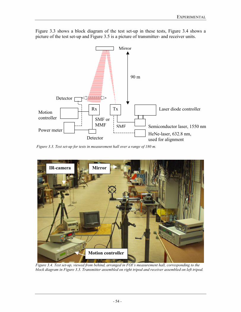
EXPERIMENTAL
- 54 -
Figure 3.3 shows a block diagram of the test set-up in these tests, Figure 3.4 shows a picture of the test set-up and Figure 3.5 is a picture of transmitter- and receiver units.
Figure 3.3. Test set-up for tests in measurement hall over a range of 180 m.
Figure 3.4. Test set-up, viewed from behind, arranged in FOI’s measurement hall, corresponding to the block diagram in Figure 3.3. Transmitter assembled on right tripod and receiver assembled on left tripod.
Semiconductor laser, 1550 nm
Laser diode controller
Mirror
HeNe-laser, 632.8 nm, used for alignment
Tx Rx
Detector
Detector
Motion controller
Power meter SMF
SMF or MMF
90 m
MirrorIR-camera
Motion controller
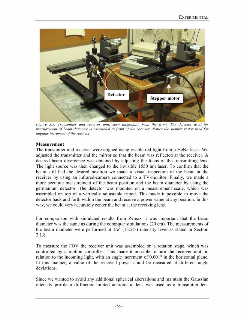
EXPERIMENTAL
- 55 -
Figure 3.5. Transmitter and receiver unit, seen diagonally from the front. The detector used for measurement of beam diameter is assembled in front of the receiver. Notice the stepper motor used for angular increment of the receiver.
Measurement The transmitter and receiver were aligned using visible red light from a HeNe-laser. We adjusted the transmitter and the mirror so that the beam was reflected at the receiver. A desired beam divergence was obtained by adjusting the focus of the transmitting lens. The light source was then changed to the invisible 1550 nm laser. To confirm that the beam still had the desired position we made a visual inspection of the beam at the receiver by using an infrared-camera connected to a TV-monitor. Finally, we made a more accurate measurement of the beam position and the beam diameter by using the germanium detector. The detector was mounted on a measurement scale, which was assembled on top of a vertically adjustable tripod. This made it possible to move the detector back and forth within the beam and receive a power value at any position. In this way, we could very accurately center the beam at the receiving lens.
For comparison with simulated results from Zemax it was important that the beam diameter was the same as during the computer simulations (20 cm). The measurements of the beam diameter were performed at 1/e2 (13.5%) intensity level as stated in Section 2.1.8. To measure the FOV the receiver unit was assembled on a rotation stage, which was controlled by a motion controller. This made it possible to turn the receiver unit, in relation to the incoming light, with an angle increment of 0.001° in the horizontal plane. In this manner, a value of the received power could be measured at different angle deviations. Since we wanted to avoid any additional spherical aberrations and maintain the Gaussian intensity profile a diffraction-limited achromatic lens was used as a transmitter lens
DetectorStepper motor
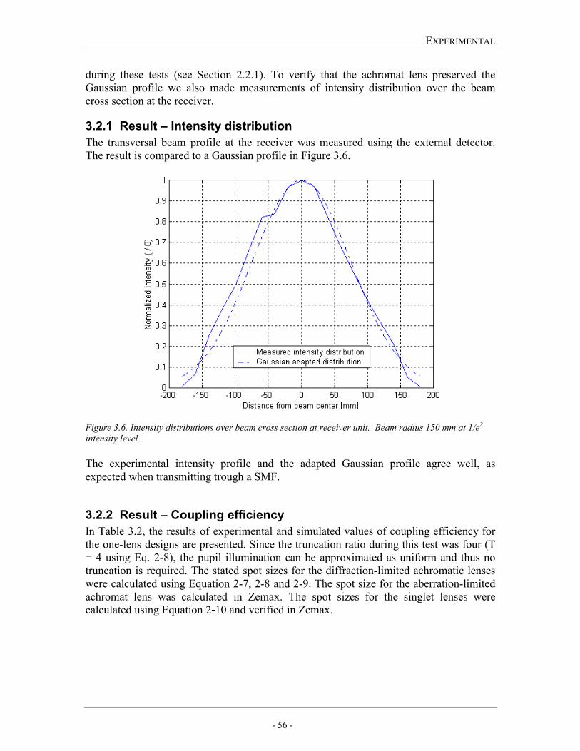
EXPERIMENTAL
- 56 -
during these tests (see Section 2.2.1). To verify that the achromat lens preserved the Gaussian profile we also made measurements of intensity distribution over the beam cross section at the receiver.
3.2.1 Result – Intensity distribution The transversal beam profile at the receiver was measured using the external detector. The result is compared to a Gaussian profile in Figure 3.6.
Figure 3.6. Intensity distributions over beam cross section at receiver unit. Beam radius 150 mm at 1/e2 intensity level. The experimental intensity profile and the adapted Gaussian profile agree well, as expected when transmitting trough a SMF.
3.2.2 Result – Coupling efficiency In Table 3.2, the results of experimental and simulated values of coupling efficiency for the one-lens designs are presented. Since the truncation ratio during this test was four (T = 4 using Eq. 2-8), the pupil illumination can be approximated as uniform and thus no truncation is required. The stated spot sizes for the diffraction-limited achromatic lenses were calculated using Equation 2-7, 2-8 and 2-9. The spot size for the aberration-limited achromat lens was calculated in Zemax. The spot sizes for the singlet lenses were calculated using Equation 2-10 and verified in Zemax.
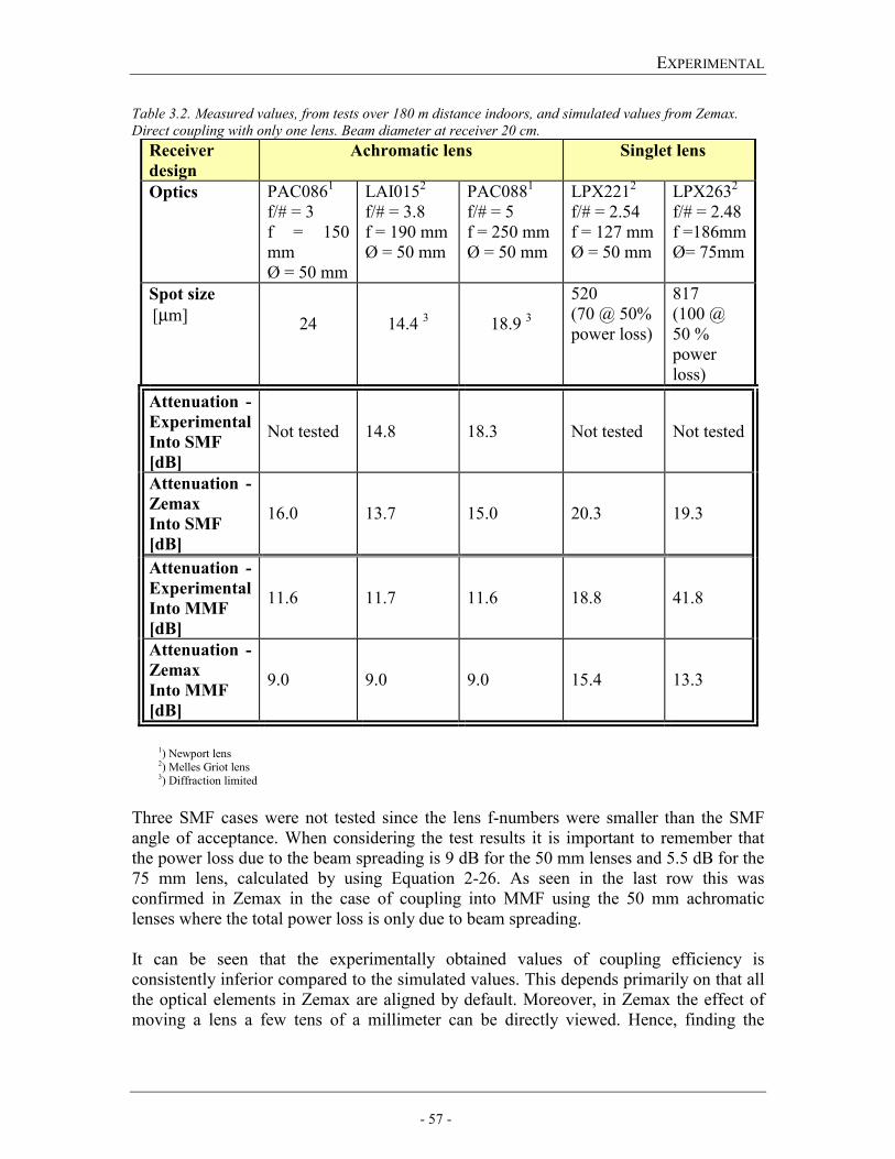
EXPERIMENTAL
- 57 -
Table 3.2. Measured values, from tests over 180 m distance indoors, and simulated values from Zemax. Direct coupling with only one lens. Beam diameter at receiver 20 cm.
Receiver design
Achromatic lens Singlet lens
Optics PAC0861
f/# = 3 f = 150 mm Ø = 50 mm
LAI0152 f/# = 3.8 f = 190 mm Ø = 50 mm
PAC0881 f/# = 5 f = 250 mm Ø = 50 mm
LPX2212 f/# = 2.54 f = 127 mm Ø = 50 mm
LPX2632 f/# = 2.48 f =186mmØ= 75mm
Spot size [µm] 24
14.4 3
18.9 3
520 (70 @ 50% power loss)
817 (100 @ 50 % power loss)
Attenuation - Experimental Into SMF [dB]
Not tested 14.8
18.3
Not tested Not tested
Attenuation - Zemax Into SMF [dB]
16.0 13.7 15.0 20.3 19.3
Attenuation - Experimental Into MMF [dB]
11.6 11.7 11.6 18.8 41.8
Attenuation - Zemax Into MMF [dB]
9.0 9.0 9.0 15.4 13.3
1) Newport lens 2) Melles Griot lens 3) Diffraction limited
Three SMF cases were not tested since the lens f-numbers were smaller than the SMF angle of acceptance. When considering the test results it is important to remember that the power loss due to the beam spreading is 9 dB for the 50 mm lenses and 5.5 dB for the 75 mm lens, calculated by using Equation 2-26. As seen in the last row this was confirmed in Zemax in the case of coupling into MMF using the 50 mm achromatic lenses where the total power loss is only due to beam spreading. It can be seen that the experimentally obtained values of coupling efficiency is consistently inferior compared to the simulated values. This depends primarily on that all the optical elements in Zemax are aligned by default. Moreover, in Zemax the effect of moving a lens a few tens of a millimeter can be directly viewed. Hence, finding the
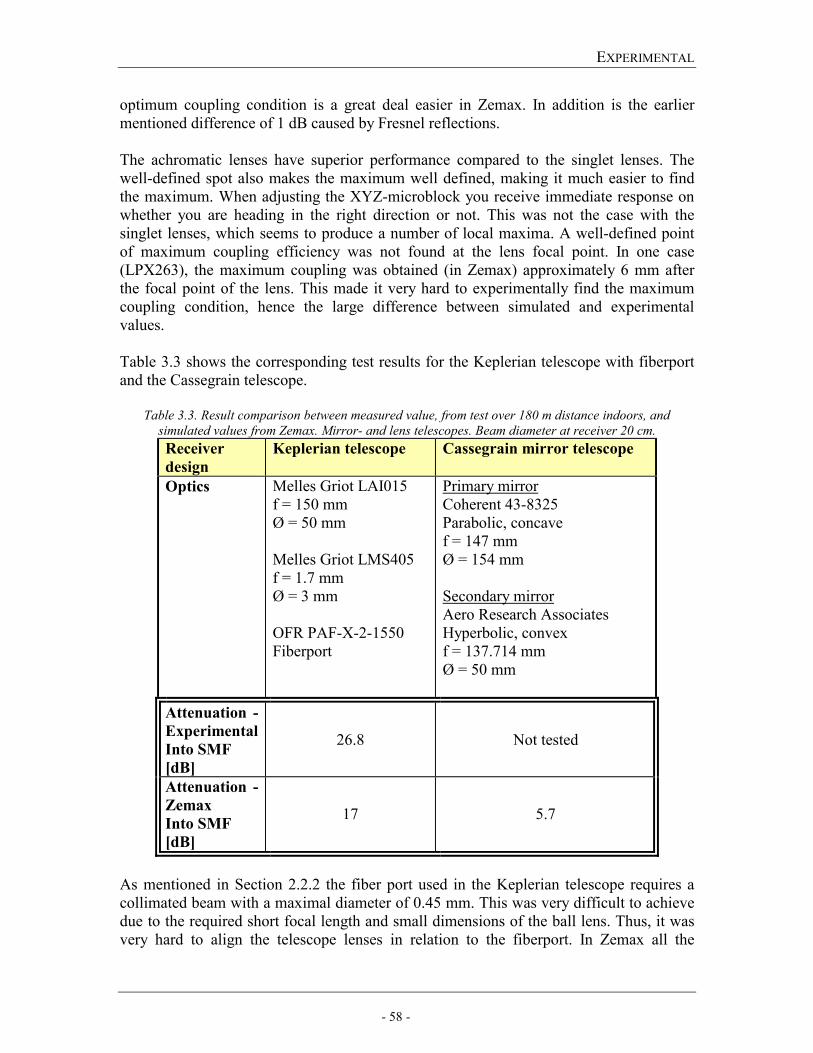
EXPERIMENTAL
- 58 -
optimum coupling condition is a great deal easier in Zemax. In addition is the earlier mentioned difference of 1 dB caused by Fresnel reflections. The achromatic lenses have superior performance compared to the singlet lenses. The well-defined spot also makes the maximum well defined, making it much easier to find the maximum. When adjusting the XYZ-microblock you receive immediate response on whether you are heading in the right direction or not. This was not the case with the singlet lenses, which seems to produce a number of local maxima. A well-defined point of maximum coupling efficiency was not found at the lens focal point. In one case (LPX263), the maximum coupling was obtained (in Zemax) approximately 6 mm after the focal point of the lens. This made it very hard to experimentally find the maximum coupling condition, hence the large difference between simulated and experimental values. Table 3.3 shows the corresponding test results for the Keplerian telescope with fiberport and the Cassegrain telescope.
Table 3.3. Result comparison between measured value, from test over 180 m distance indoors, and simulated values from Zemax. Mirror- and lens telescopes. Beam diameter at receiver 20 cm. Receiver design
Keplerian telescope Cassegrain mirror telescope
Optics Melles Griot LAI015
f = 150 mm Ø = 50 mm Melles Griot LMS405 f = 1.7 mm Ø = 3 mm OFR PAF-X-2-1550 Fiberport
Primary mirror Coherent 43-8325 Parabolic, concave f = 147 mm Ø = 154 mm Secondary mirror Aero Research Associates Hyperbolic, convex f = 137.714 mm Ø = 50 mm
Attenuation -Experimental Into SMF [dB]
26.8
Not tested
Attenuation - Zemax Into SMF [dB]
17 5.7
As mentioned in Section 2.2.2 the fiber port used in the Keplerian telescope requires a collimated beam with a maximal diameter of 0.45 mm. This was very difficult to achieve due to the required short focal length and small dimensions of the ball lens. Thus, it was very hard to align the telescope lenses in relation to the fiberport. In Zemax all the
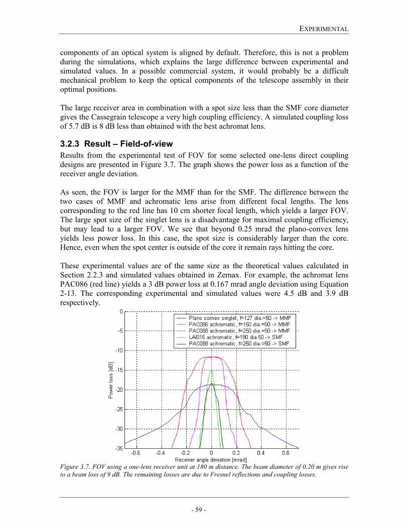
EXPERIMENTAL
- 59 -
components of an optical system is aligned by default. Therefore, this is not a problem during the simulations, which explains the large difference between experimental and simulated values. In a possible commercial system, it would probably be a difficult mechanical problem to keep the optical components of the telescope assembly in their optimal positions. The large receiver area in combination with a spot size less than the SMF core diameter gives the Cassegrain telescope a very high coupling efficiency. A simulated coupling loss of 5.7 dB is 8 dB less than obtained with the best achromat lens.
3.2.3 Result – Field-of-view Results from the experimental test of FOV for some selected one-lens direct coupling designs are presented in Figure 3.7. The graph shows the power loss as a function of the receiver angle deviation. As seen, the FOV is larger for the MMF than for the SMF. The difference between the two cases of MMF and achromatic lens arise from different focal lengths. The lens corresponding to the red line has 10 cm shorter focal length, which yields a larger FOV. The large spot size of the singlet lens is a disadvantage for maximal coupling efficiency, but may lead to a larger FOV. We see that beyond 0.25 mrad the plano-convex lens yields less power loss. In this case, the spot size is considerably larger than the core. Hence, even when the spot center is outside of the core it remain rays hitting the core. These experimental values are of the same size as the theoretical values calculated in Section 2.2.3 and simulated values obtained in Zemax. For example, the achromat lens PAC086 (red line) yields a 3 dB power loss at 0.167 mrad angle deviation using Equation 2-13. The corresponding experimental and simulated values were 4.5 dB and 3.9 dB respectively.
Figure 3.7. FOV using a one-lens receiver unit at 180 m distance. The beam diameter of 0.20 m gives rise to a beam loss of 9 dB. The remaining losses are due to Fresnel reflections and coupling losses.
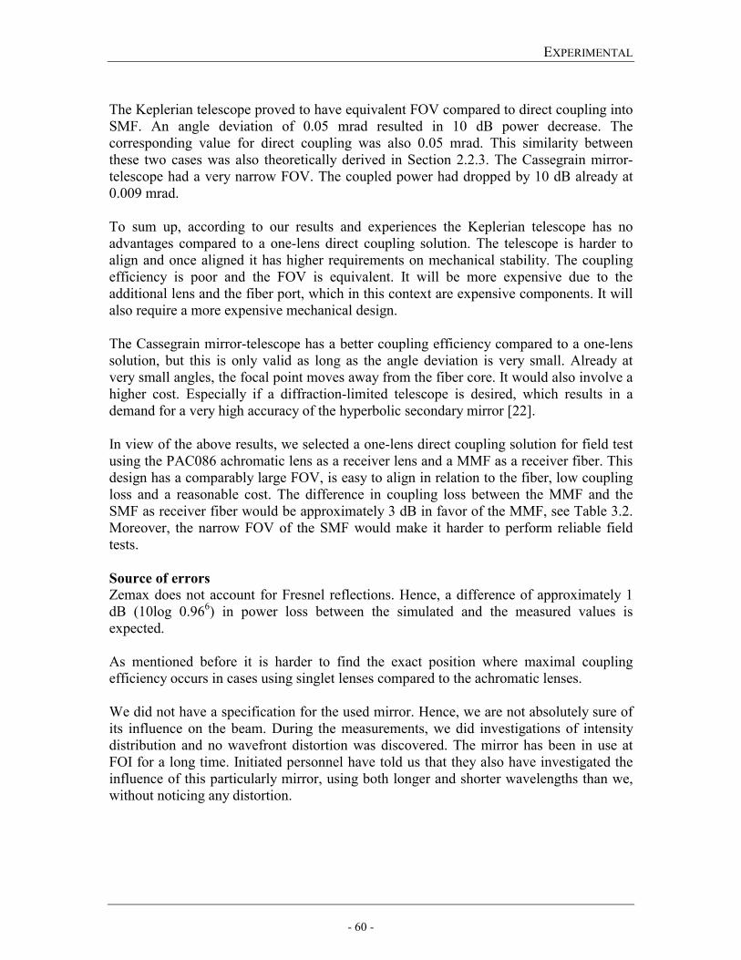
EXPERIMENTAL
- 60 -
The Keplerian telescope proved to have equivalent FOV compared to direct coupling into SMF. An angle deviation of 0.05 mrad resulted in 10 dB power decrease. The corresponding value for direct coupling was also 0.05 mrad. This similarity between these two cases was also theoretically derived in Section 2.2.3. The Cassegrain mirror-telescope had a very narrow FOV. The coupled power had dropped by 10 dB already at 0.009 mrad. To sum up, according to our results and experiences the Keplerian telescope has no advantages compared to a one-lens direct coupling solution. The telescope is harder to align and once aligned it has higher requirements on mechanical stability. The coupling efficiency is poor and the FOV is equivalent. It will be more expensive due to the additional lens and the fiber port, which in this context are expensive components. It will also require a more expensive mechanical design. The Cassegrain mirror-telescope has a better coupling efficiency compared to a one-lens solution, but this is only valid as long as the angle deviation is very small. Already at very small angles, the focal point moves away from the fiber core. It would also involve a higher cost. Especially if a diffraction-limited telescope is desired, which results in a demand for a very high accuracy of the hyperbolic secondary mirror [22]. In view of the above results, we selected a one-lens direct coupling solution for field test using the PAC086 achromatic lens as a receiver lens and a MMF as a receiver fiber. This design has a comparably large FOV, is easy to align in relation to the fiber, low coupling loss and a reasonable cost. The difference in coupling loss between the MMF and the SMF as receiver fiber would be approximately 3 dB in favor of the MMF, see Table 3.2. Moreover, the narrow FOV of the SMF would make it harder to perform reliable field tests.
Source of errors Zemax does not account for Fresnel reflections. Hence, a difference of approximately 1 dB (10log 0.966) in power loss between the simulated and the measured values is expected. As mentioned before it is harder to find the exact position where maximal coupling efficiency occurs in cases using singlet lenses compared to the achromatic lenses. We did not have a specification for the used mirror. Hence, we are not absolutely sure of its influence on the beam. During the measurements, we did investigations of intensity distribution and no wavefront distortion was discovered. The mirror has been in use at FOI for a long time. Initiated personnel have told us that they also have investigated the influence of this particularly mirror, using both longer and shorter wavelengths than we, without noticing any distortion.
EXPERIMENTAL
- 61 -
3.3 Field tests – Distance 420 m Background
We were now familiar with how the link worked without atmospheric influence. Hence, the next step was to investigate what different weather conditions, such as fog, snow and rain would do for the link performance. We were also interested in the effects of scintillations and beam wandering – and consequently if the receiver aperture was large enough. Telescopic sights were mounted on both the receiver and the transmitter unit, as help for the pre-alignment. We did also a measurement of receiver angle tolerance to verify that the value obtained indoors also was valid in real-life conditions. The transmitter unit was placed in an office at Linköping University, 420 meters away from FOI where the receiver unit was housed. The distance was measured with a laser-range finder. Figure 3.8 shows the view out from FOI. In the background, Linköping University can just be seen this day when it was a dense snowfall. The weather station used for visibility measurements etc. can be seen a few meters outside of the window.
Figure 3.8. View out from FOI, with the receiver unit facing the transmitter unit 420 meters away.
Equipment
Figure 3.9 shows an overview of the equipment used in these tests. Receiver assembly: QuickSet Hercules tripod (tiltable and turnable). Telescopic
sight mounted to the right of the lens. Detector TTI (sensitivity –83 dBm/√Hz). National Instruments data collecting card. Computer with LabView.
Receiver lens: Newport achromatic PAC086, dia. = 50 mm, f = 150 mm. Transmitter assembly: QuickSet Hercules tripod (tiltable and turnable). Telescopic
sight mounted to the right of the lens. Transmitter lens: Melles Griot, achromatic, dia. = 20 mm, f = 40 mm.
Transmitter
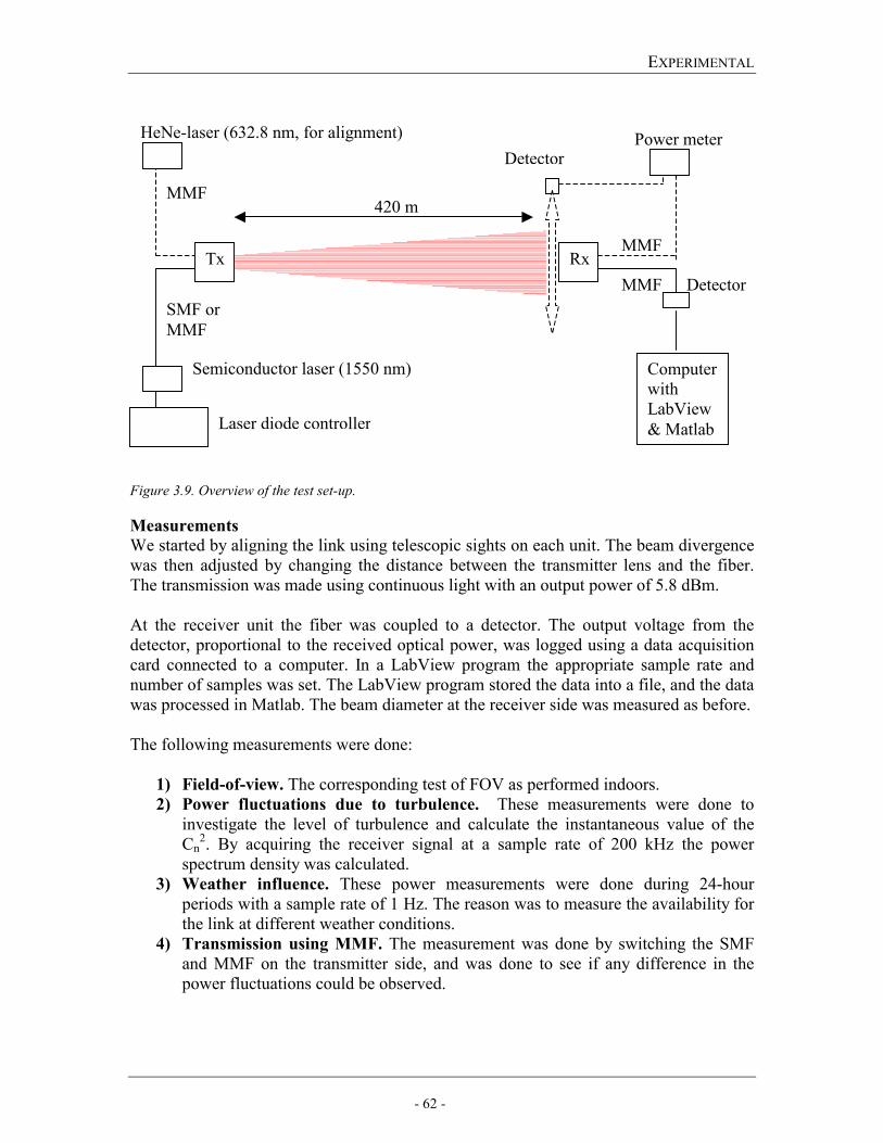
EXPERIMENTAL
- 62 -
Figure 3.9. Overview of the test set-up.
Measurements We started by aligning the link using telescopic sights on each unit. The beam divergence was then adjusted by changing the distance between the transmitter lens and the fiber. The transmission was made using continuous light with an output power of 5.8 dBm. At the receiver unit the fiber was coupled to a detector. The output voltage from the detector, proportional to the received optical power, was logged using a data acquisition card connected to a computer. In a LabView program the appropriate sample rate and number of samples was set. The LabView program stored the data into a file, and the data was processed in Matlab. The beam diameter at the receiver side was measured as before. The following measurements were done:
1) Field-of-view. The corresponding test of FOV as performed indoors. 2) Power fluctuations due to turbulence. These measurements were done to
investigate the level of turbulence and calculate the instantaneous value of the Cn
2. By acquiring the receiver signal at a sample rate of 200 kHz the power spectrum density was calculated.
3) Weather influence. These power measurements were done during 24-hour periods with a sample rate of 1 Hz. The reason was to measure the availability for the link at different weather conditions.
4) Transmission using MMF. The measurement was done by switching the SMF and MMF on the transmitter side, and was done to see if any difference in the power fluctuations could be observed.
Semiconductor laser (1550 nm)
Laser diode controller
HeNe-laser (632.8 nm, for alignment)
Tx Rx
Detector Power meter
MMF
SMF or MMF
420 m
Computer with LabView & Matlab
MMF
MMF
Detector
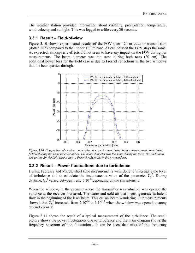
EXPERIMENTAL
- 63 -
The weather station provided information about visibility, precipitation, temperature, wind velocity and sunlight. This was logged to a file every 30 seconds.
3.3.1 Result – Field-of-view Figure 3.10 shows experimental results of the FOV over 420 m outdoor transmission (dotted line) compared to the indoor 180 m case. As can be seen the FOV stays the same. As expected, atmospheric effects did not seem to have any impact on the FOV during our measurements. The beam diameter was the same during both tests (20 cm). The additional power loss for the field case is due to Fresnel reflections in the two windows that the beam passes through.
Figure 3.10. Comparison of receiver angle tolerances performed during indoor measurement and during field test using the same receiver optics. The beam diameter was the same during the tests. The additional power loss for the field case is due to Fresnel reflections in the two windows.
3.3.2 Result – Power fluctuations due to turbulence During February and March, short time measurements were done to investigate the level of turbulence and to calculate the instantaneous value of the parameter Cn
2. During daytime, Cn
2 varied between 1 and 5⋅10-14depending on the sun intensity. When the window, in the premise where the transmitter was situated, was opened the variance at the receiver increased. The warm and cold air that meets, generate turbulent flow in the beginning of the laser beam. This causes beam wandering. Our measurements showed that Cn
2 increased from 2⋅10-14 to 1⋅10-13 when the window was opened a sunny day in February. Figure 3.11 shows the result of a typical measurement of the turbulence. The small picture shows the power fluctuations due to turbulence and the main diagram shows the frequency spectrum of the fluctuations. It can be seen that most of the frequency
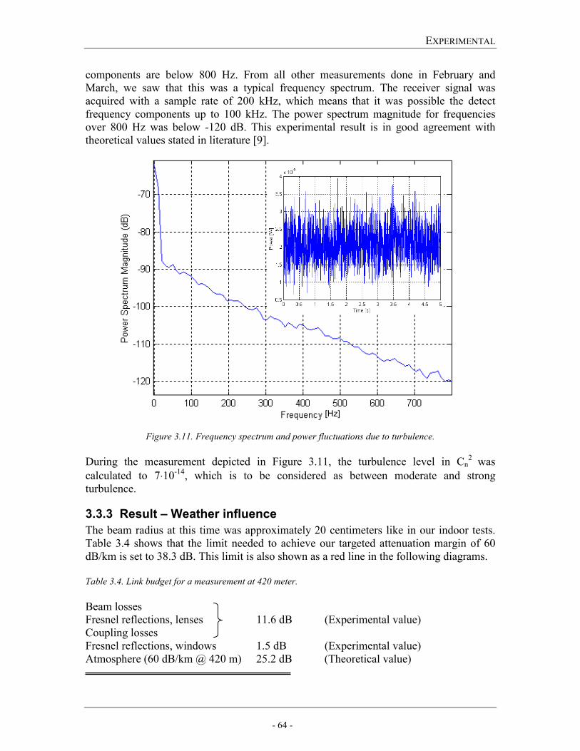
EXPERIMENTAL
- 64 -
components are below 800 Hz. From all other measurements done in February and March, we saw that this was a typical frequency spectrum. The receiver signal was acquired with a sample rate of 200 kHz, which means that it was possible the detect frequency components up to 100 kHz. The power spectrum magnitude for frequencies over 800 Hz was below -120 dB. This experimental result is in good agreement with theoretical values stated in literature [9].
Figure 3.11. Frequency spectrum and power fluctuations due to turbulence. During the measurement depicted in Figure 3.11, the turbulence level in Cn
2 was calculated to 7⋅10-14, which is to be considered as between moderate and strong turbulence.
3.3.3 Result – Weather influence The beam radius at this time was approximately 20 centimeters like in our indoor tests. Table 3.4 shows that the limit needed to achieve our targeted attenuation margin of 60 dB/km is set to 38.3 dB. This limit is also shown as a red line in the following diagrams. Table 3.4. Link budget for a measurement at 420 meter. Beam losses Fresnel reflections, lenses 11.6 dB (Experimental value) Coupling losses Fresnel reflections, windows 1.5 dB (Experimental value) Atmosphere (60 dB/km @ 420 m) 25.2 dB (Theoretical value)
[Hz]
EXPERIMENTAL
- 65 -
Link budget limit 38.3 dB
Example 1 – Influence of snowfall Figure 3.12 shows one example of the 24-hour measurements. During the first hours (time = 0 to 2 h) of the measurement, it was still warm after a day with a lot of sunshine. The fluctuations may be explained by the fact that the beam was passing a hot rooftop and therefore exposed to more turbulence during that time. At approximately 6.30 (time = 14 h) in the morning, the laser beam was interrupted during one sample (1 s). We do not find any other reason except that something has shortly broken the laser beam, probably a bird. The whole day (time = 17 to 24), it was a harsh snowfall and wind, which caused high attenuation. As seen in Figure 3.11 the visibility sometimes dropped below 1000 meters, causing high attenuation. The relative power dropped below the link budget limit when the visibility was below approximately 600 meters due to the harsh snowfall. This occurred between 2.30 and 3.00 in the afternoon (time = 22 to 22.5). It is interesting to make a comparison with Table 2.1, where it is theoretically stated that snow cannot cause an atmospheric attenuation greater than 60 dB/km. The experimental result shows that it is possible, but most likely was this high attenuation due to deposited snow on the outside of the windows.
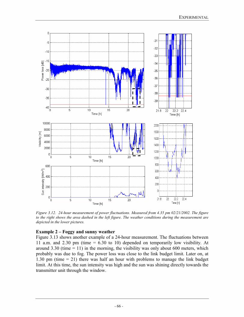
EXPERIMENTAL
- 66 -
Figure 3.12. 24-hour measurement of power fluctuations. Measured from 4.35 pm 02/21/2002. The figure to the right shows the area dashed in the left figure. The weather conditions during the measurement are depicted in the lower pictures. Example 2 – Foggy and sunny weather Figure 3.13 shows another example of a 24-hour measurement. The fluctuations between 11 a.m. and 2.30 pm (time = 6.30 to 10) depended on temporarily low visibility. At around 3.30 (time = 11) in the morning, the visibility was only about 600 meters, which probably was due to fog. The power loss was close to the link budget limit. Later on, at 1.30 pm (time = 21) there was half an hour with problems to manage the link budget limit. At this time, the sun intensity was high and the sun was shining directly towards the transmitter unit through the window.

EXPERIMENTAL
- 67 -
We are not sure of the reason for this effect, but it could be one of the following factors: • Sun shining on the transmitter assembly changing the alignment. • Beam wandering due to turbulence close to the window at the transmitter unit side. • Thermal expansion of the window, changing beam direction. After discovering this effect, we used an awning or a Venetian blind in the continuing measurements to keep the sun from shining directly at the transmitter. Since then, we have not seen such effects. Hence, this unexplained problem could probably be considered as sun-related in some way.
Figure 3.13. 24-hour measurement of power fluctuations. Measured from 4.35 pm 02/23/2002. The figure to the right shows the area dashed in the left figure. The weather conditions during the measurement are depicted in the lower pictures.
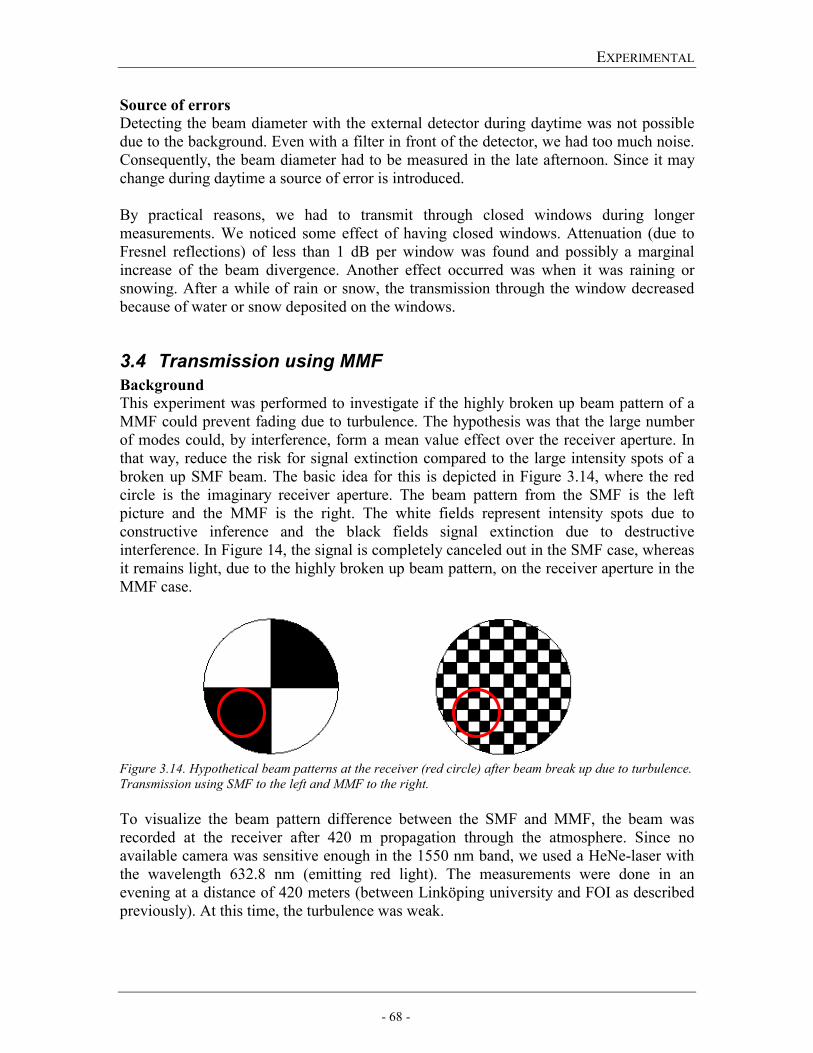
EXPERIMENTAL
- 68 -
Source of errors Detecting the beam diameter with the external detector during daytime was not possible due to the background. Even with a filter in front of the detector, we had too much noise. Consequently, the beam diameter had to be measured in the late afternoon. Since it may change during daytime a source of error is introduced. By practical reasons, we had to transmit through closed windows during longer measurements. We noticed some effect of having closed windows. Attenuation (due to Fresnel reflections) of less than 1 dB per window was found and possibly a marginal increase of the beam divergence. Another effect occurred was when it was raining or snowing. After a while of rain or snow, the transmission through the window decreased because of water or snow deposited on the windows.
3.4 Transmission using MMF Background
This experiment was performed to investigate if the highly broken up beam pattern of a MMF could prevent fading due to turbulence. The hypothesis was that the large number of modes could, by interference, form a mean value effect over the receiver aperture. In that way, reduce the risk for signal extinction compared to the large intensity spots of a broken up SMF beam. The basic idea for this is depicted in Figure 3.14, where the red circle is the imaginary receiver aperture. The beam pattern from the SMF is the left picture and the MMF is the right. The white fields represent intensity spots due to constructive inference and the black fields signal extinction due to destructive interference. In Figure 14, the signal is completely canceled out in the SMF case, whereas it remains light, due to the highly broken up beam pattern, on the receiver aperture in the MMF case. Figure 3.14. Hypothetical beam patterns at the receiver (red circle) after beam break up due to turbulence. Transmission using SMF to the left and MMF to the right. To visualize the beam pattern difference between the SMF and MMF, the beam was recorded at the receiver after 420 m propagation through the atmosphere. Since no available camera was sensitive enough in the 1550 nm band, we used a HeNe-laser with the wavelength 632.8 nm (emitting red light). The measurements were done in an evening at a distance of 420 meters (between Linköping university and FOI as described previously). At this time, the turbulence was weak.
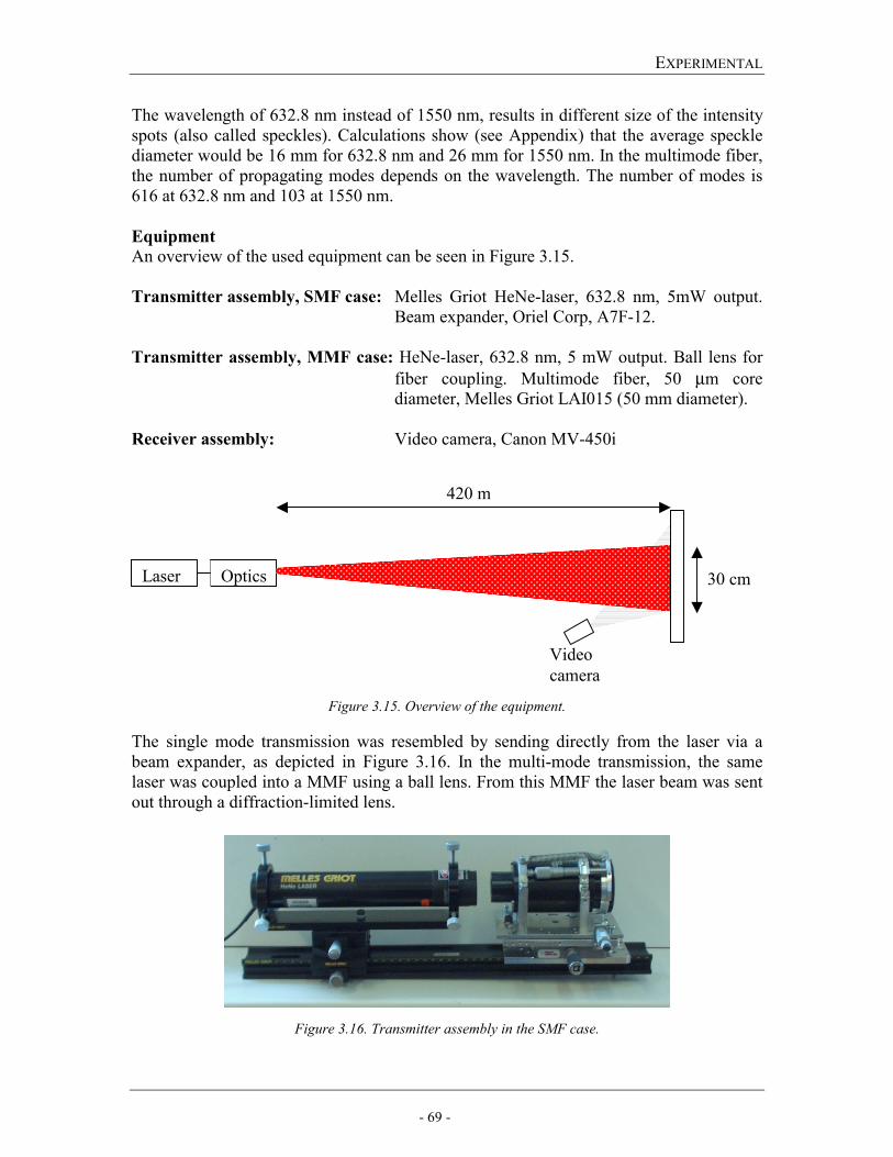
EXPERIMENTAL
- 69 -
The wavelength of 632.8 nm instead of 1550 nm, results in different size of the intensity spots (also called speckles). Calculations show (see Appendix) that the average speckle diameter would be 16 mm for 632.8 nm and 26 mm for 1550 nm. In the multimode fiber, the number of propagating modes depends on the wavelength. The number of modes is 616 at 632.8 nm and 103 at 1550 nm.
Equipment An overview of the used equipment can be seen in Figure 3.15.
Transmitter assembly, SMF case: Melles Griot HeNe-laser, 632.8 nm, 5mW output.
Beam expander, Oriel Corp, A7F-12. Transmitter assembly, MMF case: HeNe-laser, 632.8 nm, 5 mW output. Ball lens for
fiber coupling. Multimode fiber, 50 µm core diameter, Melles Griot LAI015 (50 mm diameter).
Receiver assembly: Video camera, Canon MV-450i
Figure 3.15. Overview of the equipment.
The single mode transmission was resembled by sending directly from the laser via a beam expander, as depicted in Figure 3.16. In the multi-mode transmission, the same laser was coupled into a MMF using a ball lens. From this MMF the laser beam was sent out through a diffraction-limited lens.
Figure 3.16. Transmitter assembly in the SMF case.
Optics
Video camera
420 m
30 cmLaser
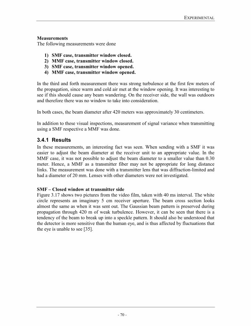
EXPERIMENTAL
- 70 -
Measurements
The following measurements were done
1) SMF case, transmitter window closed. 2) MMF case, transmitter window closed. 3) SMF case, transmitter window opened. 4) MMF case, transmitter window opened.
In the third and forth measurement there was strong turbulence at the first few meters of the propagation, since warm and cold air met at the window opening. It was interesting to see if this should cause any beam wandering. On the receiver side, the wall was outdoors and therefore there was no window to take into consideration. In both cases, the beam diameter after 420 meters was approximately 30 centimeters. In addition to these visual inspections, measurement of signal variance when transmitting using a SMF respective a MMF was done.
3.4.1 Results In these measurements, an interesting fact was seen. When sending with a SMF it was easier to adjust the beam diameter at the receiver unit to an appropriate value. In the MMF case, it was not possible to adjust the beam diameter to a smaller value than 0.30 meter. Hence, a MMF as a transmitter fiber may not be appropriate for long distance links. The measurement was done with a transmitter lens that was diffraction-limited and had a diameter of 20 mm. Lenses with other diameters were not investigated.
SMF – Closed window at transmitter side Figure 3.17 shows two pictures from the video film, taken with 40 ms interval. The white circle represents an imaginary 5 cm receiver aperture. The beam cross section looks almost the same as when it was sent out. The Gaussian beam pattern is preserved during propagation through 420 m of weak turbulence. However, it can be seen that there is a tendency of the beam to break up into a speckle pattern. It should also be understood that the detector is more sensitive than the human eye, and is thus affected by fluctuations that the eye is unable to see [35].
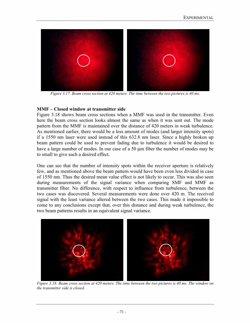
EXPERIMENTAL
- 71 -
Figure 3.17. Beam cross section at 420 meters. The time between the two pictures is 40 ms.
MMF – Closed window at transmitter side Figure 3.18 shows beam cross sections when a MMF was used in the transmitter. Even here the beam cross section looks almost the same as when it was sent out. The mode pattern from the MMF is maintained over the distance of 420 meters in weak turbulence. As mentioned earlier, there would be a less amount of modes (and larger intensity spots) if a 1550 nm laser were used instead of this 632.8 nm laser. Since a highly broken up beam pattern could be used to prevent fading due to turbulence it would be desired to have a large number of modes. In our case of a 50 µm fiber the number of modes may be to small to give such a desired effect. One can see that the number of intensity spots within the receiver aperture is relatively few, and as mentioned above the beam pattern would have been even less divided in case of 1550 nm. Thus the desired mean value effect is not likely to occur. This was also seen during measurements of the signal variance when comparing SMF and MMF as transmitter fiber. No difference, with respect to influence from turbulence, between the two cases was discovered. Several measurements were done over 420 m. The received signal with the least variance altered between the two cases. This made it impossible to come to any conclusions except that, over this distance and during weak turbulence, the two beam patterns results in an equivalent signal variance.
Figure 3.18. Beam cross section at 420 meters. The time between the two pictures is 40 ms. The window on the transmitter side is closed.
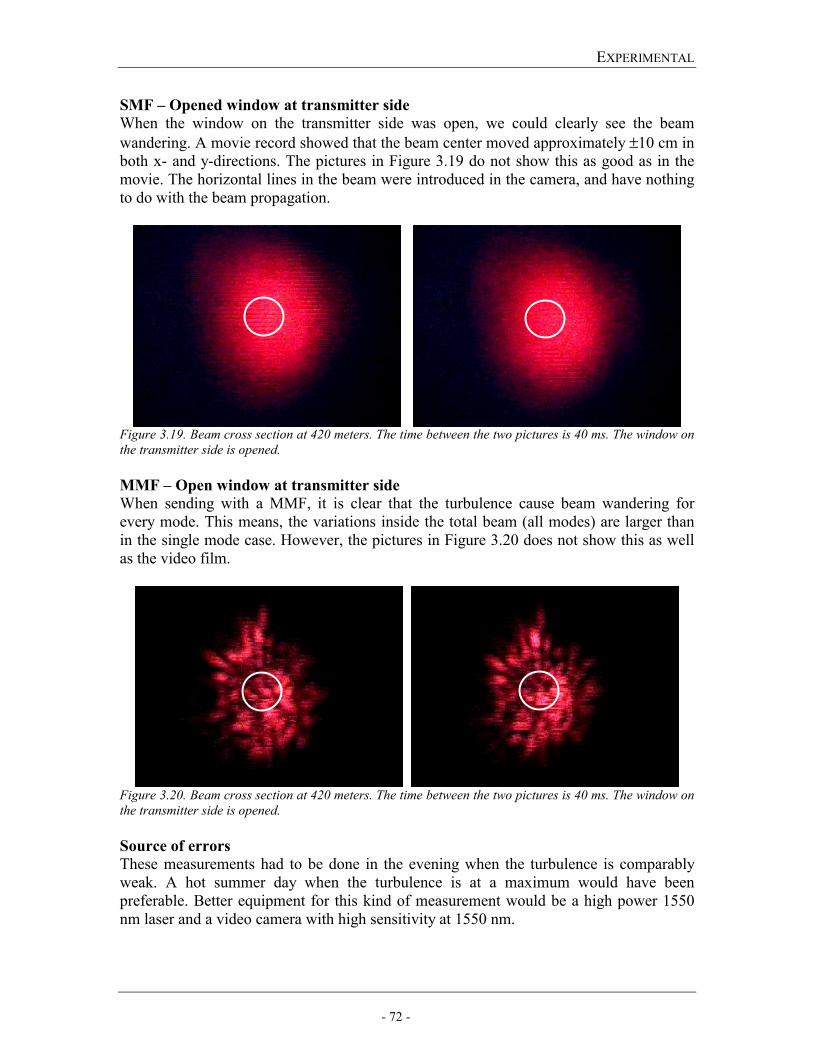
EXPERIMENTAL
- 72 -
SMF – Opened window at transmitter side When the window on the transmitter side was open, we could clearly see the beam wandering. A movie record showed that the beam center moved approximately ±10 cm in both x- and y-directions. The pictures in Figure 3.19 do not show this as good as in the movie. The horizontal lines in the beam were introduced in the camera, and have nothing to do with the beam propagation.
Figure 3.19. Beam cross section at 420 meters. The time between the two pictures is 40 ms. The window on the transmitter side is opened. MMF – Open window at transmitter side When sending with a MMF, it is clear that the turbulence cause beam wandering for every mode. This means, the variations inside the total beam (all modes) are larger than in the single mode case. However, the pictures in Figure 3.20 does not show this as well as the video film.
Figure 3.20. Beam cross section at 420 meters. The time between the two pictures is 40 ms. The window on the transmitter side is opened.
Source of errors These measurements had to be done in the evening when the turbulence is comparably weak. A hot summer day when the turbulence is at a maximum would have been preferable. Better equipment for this kind of measurement would be a high power 1550 nm laser and a video camera with high sensitivity at 1550 nm.
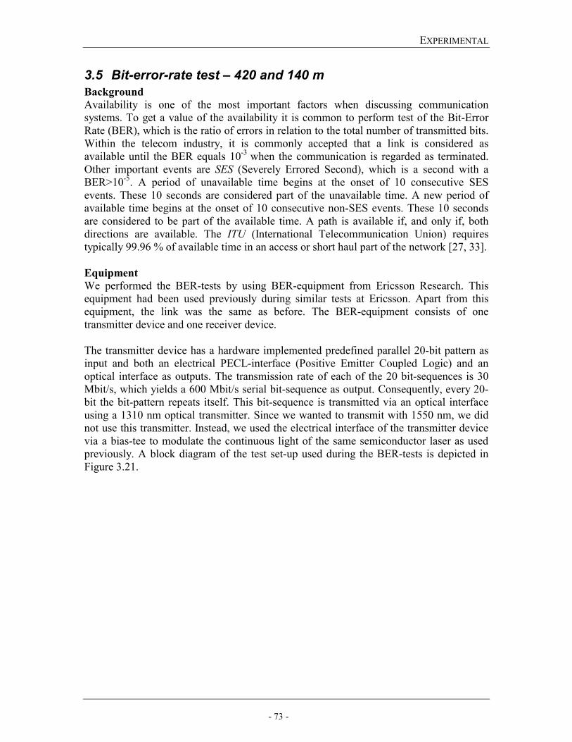
EXPERIMENTAL
- 73 -
3.5 Bit-error-rate test – 420 and 140 m Background
Availability is one of the most important factors when discussing communication systems. To get a value of the availability it is common to perform test of the Bit-Error Rate (BER), which is the ratio of errors in relation to the total number of transmitted bits. Within the telecom industry, it is commonly accepted that a link is considered as available until the BER equals 10-3 when the communication is regarded as terminated. Other important events are SES (Severely Errored Second), which is a second with a BER>10-5. A period of unavailable time begins at the onset of 10 consecutive SES events. These 10 seconds are considered part of the unavailable time. A new period of available time begins at the onset of 10 consecutive non-SES events. These 10 seconds are considered to be part of the available time. A path is available if, and only if, both directions are available. The ITU (International Telecommunication Union) requires typically 99.96 % of available time in an access or short haul part of the network [27, 33].
Equipment We performed the BER-tests by using BER-equipment from Ericsson Research. This equipment had been used previously during similar tests at Ericsson. Apart from this equipment, the link was the same as before. The BER-equipment consists of one transmitter device and one receiver device. The transmitter device has a hardware implemented predefined parallel 20-bit pattern as input and both an electrical PECL-interface (Positive Emitter Coupled Logic) and an optical interface as outputs. The transmission rate of each of the 20 bit-sequences is 30 Mbit/s, which yields a 600 Mbit/s serial bit-sequence as output. Consequently, every 20-bit the bit-pattern repeats itself. This bit-sequence is transmitted via an optical interface using a 1310 nm optical transmitter. Since we wanted to transmit with 1550 nm, we did not use this transmitter. Instead, we used the electrical interface of the transmitter device via a bias-tee to modulate the continuous light of the same semiconductor laser as used previously. A block diagram of the test set-up used during the BER-tests is depicted in Figure 3.21.
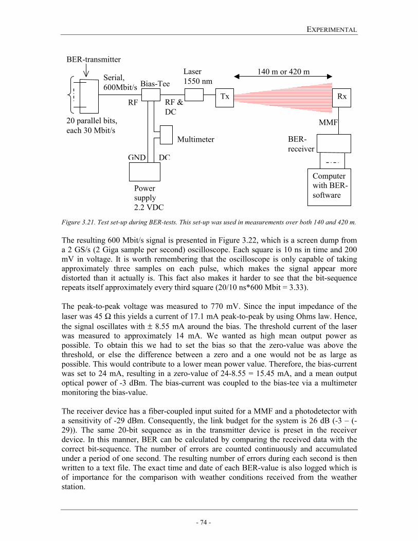
EXPERIMENTAL
- 74 -
Figure 3.21. Test set-up during BER-tests. This set-up was used in measurements over both 140 and 420 m. The resulting 600 Mbit/s signal is presented in Figure 3.22, which is a screen dump from a 2 GS/s (2 Giga sample per second) oscilloscope. Each square is 10 ns in time and 200 mV in voltage. It is worth remembering that the oscilloscope is only capable of taking approximately three samples on each pulse, which makes the signal appear more distorted than it actually is. This fact also makes it harder to see that the bit-sequence repeats itself approximately every third square (20/10 ns*600 Mbit = 3.33). The peak-to-peak voltage was measured to 770 mV. Since the input impedance of the laser was 45 Ω this yields a current of 17.1 mA peak-to-peak by using Ohms law. Hence, the signal oscillates with ± 8.55 mA around the bias. The threshold current of the laser was measured to approximately 14 mA. We wanted as high mean output power as possible. To obtain this we had to set the bias so that the zero-value was above the threshold, or else the difference between a zero and a one would not be as large as possible. This would contribute to a lower mean power value. Therefore, the bias-current was set to 24 mA, resulting in a zero-value of 24-8.55 = 15.45 mA, and a mean output optical power of -3 dBm. The bias-current was coupled to the bias-tee via a multimeter monitoring the bias-value. The receiver device has a fiber-coupled input suited for a MMF and a photodetector with a sensitivity of -29 dBm. Consequently, the link budget for the system is 26 dB (-3 – (-29)). The same 20-bit sequence as in the transmitter device is preset in the receiver device. In this manner, BER can be calculated by comparing the received data with the correct bit-sequence. The number of errors are counted continuously and accumulated under a period of one second. The resulting number of errors during each second is then written to a text file. The exact time and date of each BER-value is also logged which is of importance for the comparison with weather conditions received from the weather station.
Tx Rx
140 m or 420 m
Computer with BER- software
MMF
BER-receiver
20 parallel bits, each 30 Mbit/s
Power supply 2.2 VDC
Serial, 600Mbit/s
Multimeter
GND DC
BER-transmitter
Bias-TeeLaser 1550 nm
RF RF & DC
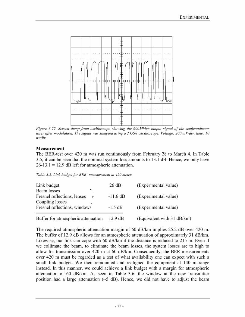
EXPERIMENTAL
- 75 -
Figure 3.22. Screen dump from oscilloscope showing the 600Mbit/s output signal of the semiconductor laser after modulation. The signal was sampled using a 2 GS/s oscilloscope. Voltage: 200 mV/div, time: 10 ns/div.
Measurement
The BER-test over 420 m was run continuously from February 28 to March 4. In Table 3.5, it can be seen that the nominal system loss amounts to 13.1 dB. Hence, we only have 26-13.1 = 12.9 dB left for atmospheric attenuation. Table 3.5. Link budget for BER- measurement at 420 meter. Link budget 26 dB (Experimental value) Beam losses Fresnel reflections, lenses -11.6 dB (Experimental value) Coupling losses Fresnel reflections, windows -1.5 dB (Experimental value) Buffer for atmospheric attenuation 12.9 dB (Equivalent with 31 dB/km) The required atmospheric attenuation margin of 60 dB/km implies 25.2 dB over 420 m. The buffer of 12.9 dB allows for an atmospheric attenuation of approximately 31 dB/km. Likewise, our link can cope with 60 dB/km if the distance is reduced to 215 m. Even if we collimate the beam, to eliminate the beam losses, the system losses are to high to allow for transmission over 420 m at 60 dB/km. Consequently, the BER-measurements over 420 m must be regarded as a test of what availability one can expect with such a small link budget. We then remounted and realigned the equipment at 140 m range instead. In this manner, we could achieve a link budget with a margin for atmospheric attenuation of 60 dB/km. As seen in Table 3.6, the window at the new transmitter position had a large attenuation (~5 dB). Hence, we did not have to adjust the beam
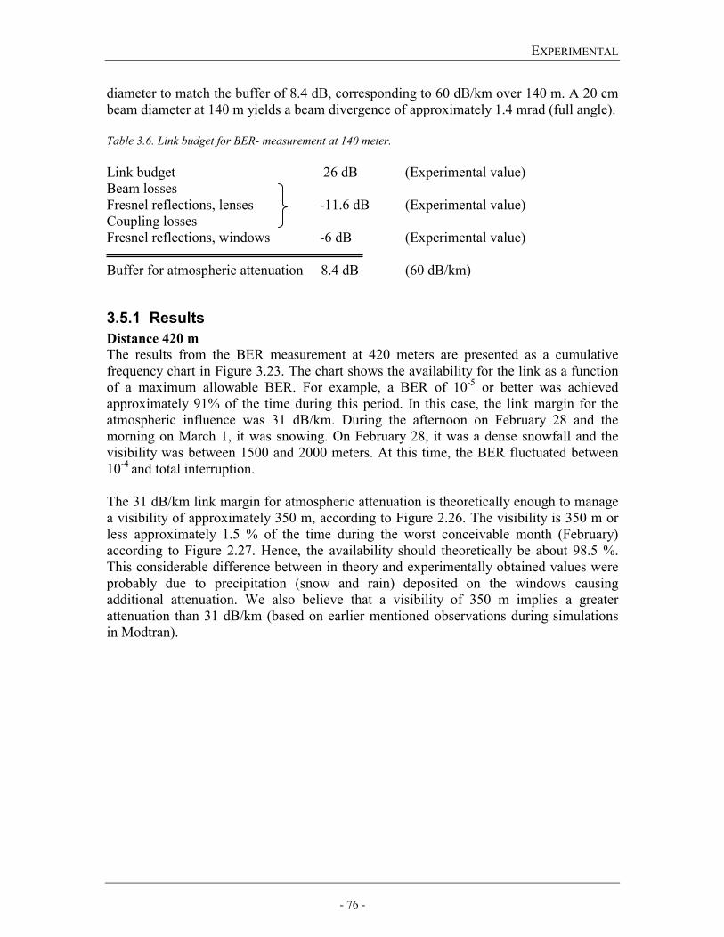
EXPERIMENTAL
- 76 -
diameter to match the buffer of 8.4 dB, corresponding to 60 dB/km over 140 m. A 20 cm beam diameter at 140 m yields a beam divergence of approximately 1.4 mrad (full angle). Table 3.6. Link budget for BER- measurement at 140 meter. Link budget 26 dB (Experimental value) Beam losses Fresnel reflections, lenses -11.6 dB (Experimental value) Coupling losses Fresnel reflections, windows -6 dB (Experimental value) Buffer for atmospheric attenuation 8.4 dB (60 dB/km)
3.5.1 Results Distance 420 m
The results from the BER measurement at 420 meters are presented as a cumulative frequency chart in Figure 3.23. The chart shows the availability for the link as a function of a maximum allowable BER. For example, a BER of 10-5 or better was achieved approximately 91% of the time during this period. In this case, the link margin for the atmospheric influence was 31 dB/km. During the afternoon on February 28 and the morning on March 1, it was snowing. On February 28, it was a dense snowfall and the visibility was between 1500 and 2000 meters. At this time, the BER fluctuated between 10-4 and total interruption. The 31 dB/km link margin for atmospheric attenuation is theoretically enough to manage a visibility of approximately 350 m, according to Figure 2.26. The visibility is 350 m or less approximately 1.5 % of the time during the worst conceivable month (February) according to Figure 2.27. Hence, the availability should theoretically be about 98.5 %. This considerable difference between in theory and experimentally obtained values were probably due to precipitation (snow and rain) deposited on the windows causing additional attenuation. We also believe that a visibility of 350 m implies a greater attenuation than 31 dB/km (based on earlier mentioned observations during simulations in Modtran).
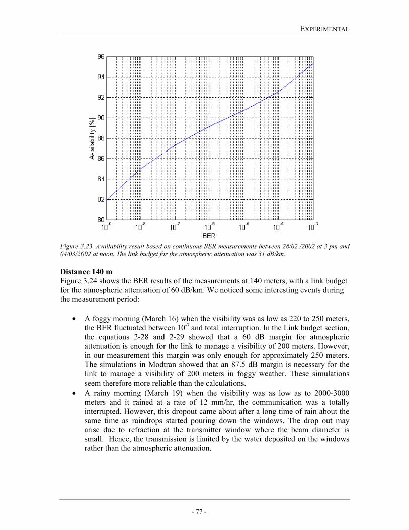
EXPERIMENTAL
- 77 -
Figure 3.23. Availability result based on continuous BER-measurements between 28/02 /2002 at 3 pm and 04/03/2002 at noon. The link budget for the atmospheric attenuation was 31 dB/km. Distance 140 m Figure 3.24 shows the BER results of the measurements at 140 meters, with a link budget for the atmospheric attenuation of 60 dB/km. We noticed some interesting events during the measurement period:
• A foggy morning (March 16) when the visibility was as low as 220 to 250 meters, the BER fluctuated between 10-7 and total interruption. In the Link budget section, the equations 2-28 and 2-29 showed that a 60 dB margin for atmospheric attenuation is enough for the link to manage a visibility of 200 meters. However, in our measurement this margin was only enough for approximately 250 meters. The simulations in Modtran showed that an 87.5 dB margin is necessary for the link to manage a visibility of 200 meters in foggy weather. These simulations seem therefore more reliable than the calculations.
• A rainy morning (March 19) when the visibility was as low as to 2000-3000 meters and it rained at a rate of 12 mm/hr, the communication was a totally interrupted. However, this dropout came about after a long time of rain about the same time as raindrops started pouring down the windows. The drop out may arise due to refraction at the transmitter window where the beam diameter is small. Hence, the transmission is limited by the water deposited on the windows rather than the atmospheric attenuation.
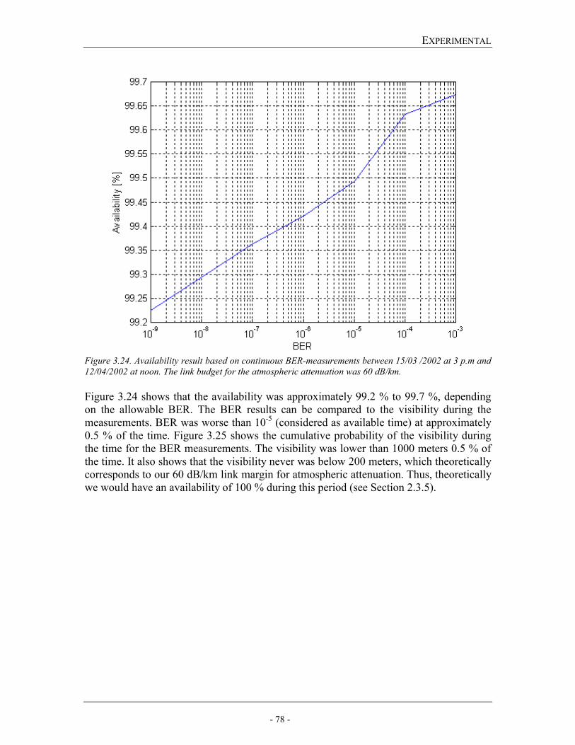
EXPERIMENTAL
- 78 -
Figure 3.24. Availability result based on continuous BER-measurements between 15/03 /2002 at 3 p.m and 12/04/2002 at noon. The link budget for the atmospheric attenuation was 60 dB/km. Figure 3.24 shows that the availability was approximately 99.2 % to 99.7 %, depending on the allowable BER. The BER results can be compared to the visibility during the measurements. BER was worse than 10-5 (considered as available time) at approximately 0.5 % of the time. Figure 3.25 shows the cumulative probability of the visibility during the time for the BER measurements. The visibility was lower than 1000 meters 0.5 % of the time. It also shows that the visibility never was below 200 meters, which theoretically corresponds to our 60 dB/km link margin for atmospheric attenuation. Thus, theoretically we would have an availability of 100 % during this period (see Section 2.3.5).
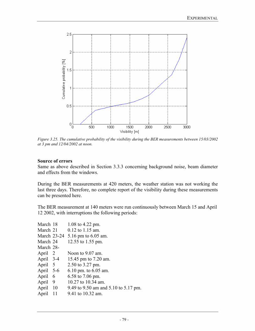
EXPERIMENTAL
- 79 -
Figure 3.25. The cumulative probability of the visibility during the BER measurements between 15/03/2002 at 3 pm and 12/04/2002 at noon.
Source of errors Same as above described in Section 3.3.3 concerning background noise, beam diameter and effects from the windows. During the BER measurements at 420 meters, the weather station was not working the last three days. Therefore, no complete report of the visibility during these measurements can be presented here. The BER measurement at 140 meters were run continuously between March 15 and April 12 2002, with interruptions the following periods: March 18 1.08 to 4.22 pm. March 21 0.12 to 1.15 am. March 23-24 5.16 pm to 6.05 am. March 24 12.55 to 1.55 pm. March 28- April 2 Noon to 9.07 am. April 3-4 15.45 pm to 7.20 am. April 5 2.50 to 3.27 pm. April 5-6 6.10 pm. to 6.05 am. April 6 6.58 to 7.06 pm. April 9 10.27 to 10.34 am. April 10 9.49 to 9.50 am and 5.10 to 5.17 pm. April 11 9.41 to 10.32 am.
EXPERIMENTAL
- 80 -
These interruptions are excluded in Figure 3.22. The interruptions above came about because of the human factor when people happened to touch the equipment causing misalignment of the system, or occurred at a time when we were not able to notice the reason for the interruption. The time of the interruptions were correlated with the data from the weather station and none of the disconnections can be derived from low visibility, precipitation or turbulence related effects. Power failure may have caused the interruptions at night. The availability presented in this section is calculated relative the time between March 15 and April 12, except from the interruptions described above.
CONCLUSION
- 81 -
4 Conclusion Transmitter fiber
We have found some advantages of using a SMF rather than a MMF in the transmitter side. At long distances (400 meter), it may be difficult to focus the beam to an appropriate diameter when a MMF is used. The Gaussian profile from the SMF makes it comparably easy to find the link alignment compared to the profile from the MMF, where many modes form a pattern of intensity spots. The SMF has also less spectral attenuation, which is desired when the light have to propagate some distance in the fiber before being transmitted through air.
Transmitter optics A diffraction-limited lens is preferable as the transmitter optics. We used standard achromats with a diameter of 20 millimeters as transmitter lenses, which functioned well. An aspheric lens with a suitable f/# could be designed, but it may not be worth the additional design expense because the standard achromats manage the task equally well.
Beam divergence and range There is a connection between the beam divergence of the transmitter and the field-of-view (angle tolerances) of the receiver unit. Hence, if the link head moves (e.g. by building movements) both the transmitted beam and the receiver directions may be altered. To avoid unnecessary power losses, the beam divergence can be adjusted to suit the receiver FOV.
Because of the narrow receiver FOV, the beam divergence should not exceed
approximately 0.8 mrad. By calculations of a link budget, this implies a maximum link range of 300 meters in case of a 5 centimetres receiver aperture diameter. If the link should manage longer distances the receiver aperture has to be larger. A range of 400 meters can be achieved using a 10 cm aperture lens and a beam divergence of 0.6 mrad. The maximum range depends on the desired availability. For example, if the demand for 99.96 % of available time stated by the ITU (International Telecommunication Union) for an access or short haul part of the network is to be fulfilled the maximum range is greatly reduced. According to Figure 2.27, the link has to manage an extremely bad visibility of approximately 7 m. This visibility yields an atmospheric attenuation around 2000 dB/km (using Eq. 2-28 and 2-29), which in turn would give a maximum link distance in the region of 15 m. However, it should be noted that this is a theoretical value and the visibility will never be as low as 7 m in real-life conditions. Although the theoretical maximum link distance values above suffer from large errors to the statistical uncertainty, these numbers imply that ITU compliant FSO links can hardly be deployed over distances more than 100 meters or less in a country like Sweden.
CONCLUSION
- 82 -
Receiver optics None of the conceivable optic designs proved to be superior compared to the straightforward one-lens solution. This was an appealing result, since it is undoubtedly the least expensive design. The Cassegrain telescope had a higher coupling efficiency, in theory, but the field-of-view is very narrow. Such a narrow FOV implies a complicated alignment and once aligned high requirements on mechanical immovability. Moreover, according to information received during the work a Cassegrain telescope, with high accuracy, is one of the most costly designs. If the link has to manage a distance of 400 meters, there is a need of a large lens diameter, preferably around 10 centimeters. We have not found standard lenses larger than 5 cm, where the spot size is diffraction-limited and suitable for this all-optical case. An aspheric singlet lens with the correct f/# of 2.5, suitable for the NA = 0.20 of a MMF, could be designed so that the spot size would be diffraction-limited (to 9.5 µm). The FOV of the receiver in this case would be approximately ±0.2 mrad. The price of designing and producing such aspheric lenses depends on the quantity. The design of a lens for coupling into a SMF is more difficult, because a SMF has a smaller core diameter (around 9 µm) and a smaller NA (around 0.13). It is possible to adjust the f/# of a lens to the NA of a SMF so that almost 100% is coupled into the fiber. However, with practically no tolerances for misalignment of the receiver unit.
Receiver fiber A fiber with large core diameter relief the alignment tolerances of the receiver unit and increases the FOV. MMF with a core diameter of 50 µm is standard in LAN applications, so most likely that diameter has to be chosen. We believe that coupling into a SMF is not practically viable, unless some kind of adaptive control compensating for misalignment of the receiver is applied to the system.
Wavelength The atmospheric transmission in the wavelength bands around 850 and 1550 nm is much the same. Our simulations showed that the transmission in fog was slightly better at 850 nm. The transceivers for 850 nm are also cheaper than the transceivers for 1550 nm. On the other hand, the fact that 1550 nm is eye-safe may be more important than cost and transmission.
Lens coating Anti-reflection coatings are expensive, especially for lenses manufactured in short production runs. It may not be worth the cost in this application. For a system with one transmitter lens and one receiver lens, it means only an attenuation of 0.7 dB.
Availability In our measurements, problems with the link connection occurred not only in foggy weather, but also when it was raining or snowing. The transmission in precipitation is limited by the water or snow deposited on the windows rather than the atmospheric
CONCLUSION
- 83 -
attenuation. This may be avoided using a roof over the transmitter and receiver aperture (or an awning outside the window if the link is used transmitting through windows). In that case, it is only fog that will cause interruptions of the transmission. Our measurements show that a 60 dB/km atmospheric attenuation margin in the link budget is enough for a link to manage a visibility of approximately 250 meters in foggy weather. During our test period (March 15 to April 12 2002) we had an availability of 99.5 %, for BER < 10-5.
- 84 -
5 References [1] http://www.freespaceoptic.com/Fiber_Optics_Without_Fiber.htm, downloaded
011112 [2] http://www.fsona.com/technology.php?sec=fso_primer, downloaded 011112 [3] http://www.fsona.com/technology.php?sec=white_papers, downloaded 011112 [4] http://filebox.vt.edu/users/yiyang1/Description.htm, downloaded 011114 [5] Merrill Lynch, Free Space Optics, 8 May 2001 [6] Mark Steege, GSEC, Free-Space Optics: A Viable, Secure Last-Mile Solution? [7] Isaac I. Kim et al, Wireless optical transmission of Fast Ethernet, FDDI, ATM,
and ESCON protocol data using the TerraLink laser communication system., Optical Engineering, Vol. 37 No. 12, December 1998
[8] http://www.freespacecoms.com/html/faq's/, downloaded 011112 [9] Bolander G., et al., December 1999, Fri optisk kommunikation – En förstudie,
FOA, Linköping, ISSN 1104-9154 [10] Pedrotti F. L., Pedrotti L. S., 1993, Introduction to optics, Second Edition,
Prentice Hall, New Jersey, ISBN 0-13-501545-6 [11] Melles Griot 1997-1998, USA, product catalogue [12] www.ludd.luth.se/~kavli/paraxial.html, downloaded 011127 [13] Tell, Andersson, Andersson, 1990, Fiberoptisk kommunikationsteknik, ISBN 91-
44-26202-7 [14] http://www.pti-nj.com/obb_fiber3.html, downloaded 011127 [15] http://www.fti.thomasregister.com/olc/fti/fiber1.htm, downloaded 011127 [16] Hewlett-Packard GmbH, 1989, Fiber Optics Handbook, Instruments Division
Boeblingen [17] C.Yeh, 1990, Handbook of fiber optics – Theory and applications, ISBN 0-
12770455-8 [18] http://www.occfiber.com/wpglass.html, downloaded 011127
- 85 -
[19] Saleh E. A. B., Teich M. C., 1991, Fundamentals of Photonics, John Wiley &
Sons INC, USA, ISBN 0-471-83965-5 [20] www.mellesgriot.com, downloaded 011108 [21] OFR, Optics for Research, 1998, New Jersey, product catalogue [22] Wetherell W.B., Rimmer M.P., 1972, General Analysis of Aplanatic Cassegrain,
Gregorian and Schwarzhild Telescopes, Applied Optics, Vol. 11, No. 12 [23] Mannberg G., Senior lecturer in optical design, Royal Institute of Technology,
KTH, Stockholm, 2002, Personal communication. [24] Byström A., Sales Engineer, Melles Griot, Stockholm, 2002, Personal
communication [25] Thorlabs, Product catalogue, 2002, Volume 14 [26] Wave optics, Specialty Fiber Optic Products, 1997, USA [27] Kallstenius T., 2002, Personal communication [28] Ericsson A., Dec 1993, Turbulence constant dependence on meteorological
parameters, Swedish Defence Research Agency (FOI), FOA D 30751-3.1 [29] Steinvall O., 1997, Theory for Laser systems performance modeling, Swedish
Defence Research Agency (FOI), ISSN 1104-9154 [30] Andrew L. C., Phillips R. L., 1998, Laser Beam Propagation through Random
Media, SPIE, Optical Engineering Press [31] Corning Optical Fiber, Product information for Singlemode and Multimode
Optical Fibers, USA [32] Melles Griot Optics Guide 5, 1990, USA [33] www.itu.int, The International Telecommunication Union, downloaded 020304 [34] Steinvall O., 2001, Reduktion av turbulensfädning hos
laserkommunikationslänkar, Swedish Defence Research Agency (FOI), ISSN 1650-1942 [35] Kullander F., 2002, Personal communication [36] www.cablefreesolutions.com/news.htm#2pt7Gig, downloaded 020429
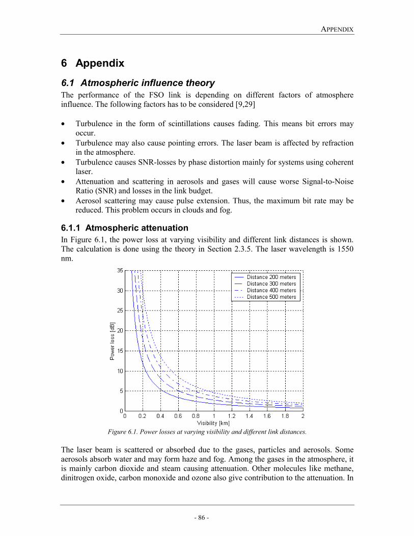
APPENDIX
- 86 -
6 Appendix
6.1 Atmospheric influence theory The performance of the FSO link is depending on different factors of atmosphere influence. The following factors has to be considered [9,29] • Turbulence in the form of scintillations causes fading. This means bit errors may
occur. • Turbulence may also cause pointing errors. The laser beam is affected by refraction
in the atmosphere. • Turbulence causes SNR-losses by phase distortion mainly for systems using coherent
laser. • Attenuation and scattering in aerosols and gases will cause worse Signal-to-Noise
Ratio (SNR) and losses in the link budget. • Aerosol scattering may cause pulse extension. Thus, the maximum bit rate may be
reduced. This problem occurs in clouds and fog.
6.1.1 Atmospheric attenuation In Figure 6.1, the power loss at varying visibility and different link distances is shown. The calculation is done using the theory in Section 2.3.5. The laser wavelength is 1550 nm.
Figure 6.1. Power losses at varying visibility and different link distances.
The laser beam is scattered or absorbed due to the gases, particles and aerosols. Some aerosols absorb water and may form haze and fog. Among the gases in the atmosphere, it is mainly carbon dioxide and steam causing attenuation. Other molecules like methane, dinitrogen oxide, carbon monoxide and ozone also give contribution to the attenuation. In
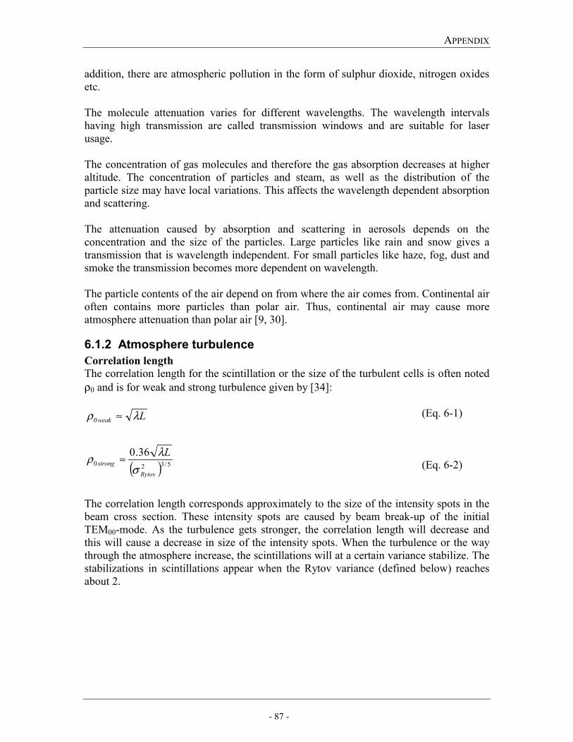
APPENDIX
- 87 -
addition, there are atmospheric pollution in the form of sulphur dioxide, nitrogen oxides etc. The molecule attenuation varies for different wavelengths. The wavelength intervals having high transmission are called transmission windows and are suitable for laser usage. The concentration of gas molecules and therefore the gas absorption decreases at higher altitude. The concentration of particles and steam, as well as the distribution of the particle size may have local variations. This affects the wavelength dependent absorption and scattering. The attenuation caused by absorption and scattering in aerosols depends on the concentration and the size of the particles. Large particles like rain and snow gives a transmission that is wavelength independent. For small particles like haze, fog, dust and smoke the transmission becomes more dependent on wavelength. The particle contents of the air depend on from where the air comes from. Continental air often contains more particles than polar air. Thus, continental air may cause more atmosphere attenuation than polar air [9, 30].
6.1.2 Atmosphere turbulence Correlation length
The correlation length for the scintillation or the size of the turbulent cells is often noted ρ0 and is for weak and strong turbulence given by [34]: (Eq. 6-1) (Eq. 6-2) The correlation length corresponds approximately to the size of the intensity spots in the beam cross section. These intensity spots are caused by beam break-up of the initial TEM00-mode. As the turbulence gets stronger, the correlation length will decrease and this will cause a decrease in size of the intensity spots. When the turbulence or the way through the atmosphere increase, the scintillations will at a certain variance stabilize. The stabilizations in scintillations appear when the Rytov variance (defined below) reaches about 2.
( ) 5/320
0
36.0
Rytovstrong
weak
L
L
σλρ
λρ
≈
≈
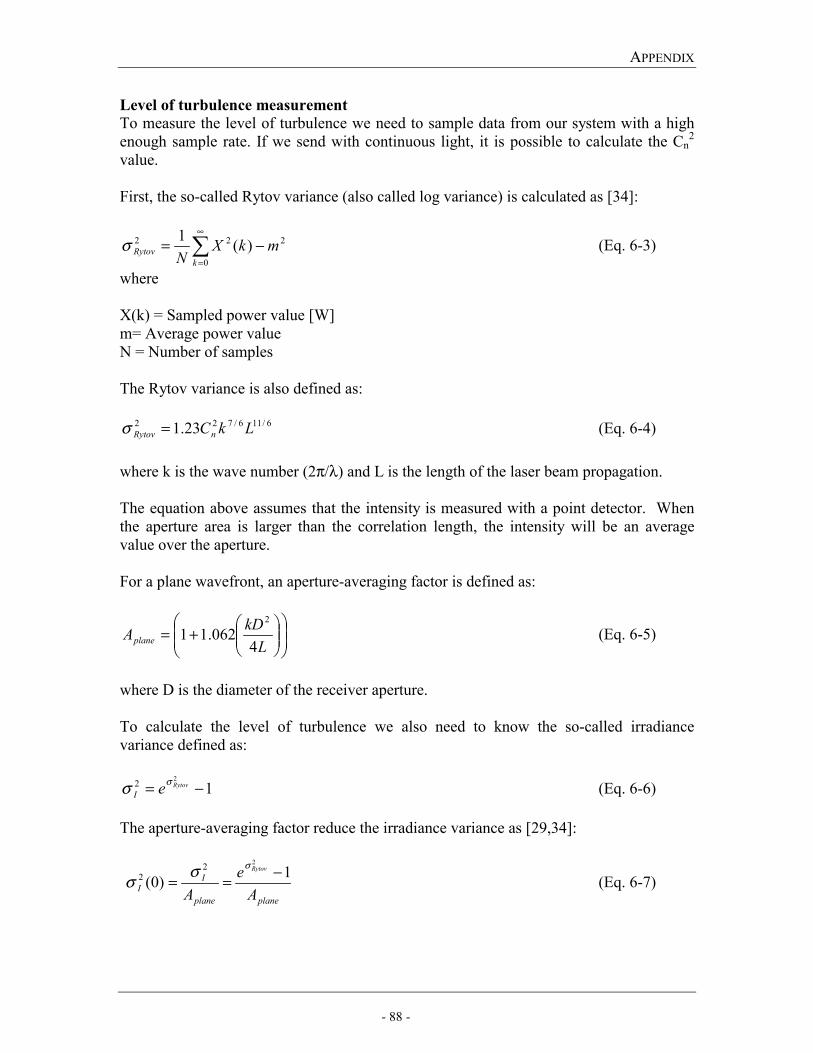
APPENDIX
- 88 -
Level of turbulence measurement To measure the level of turbulence we need to sample data from our system with a high enough sample rate. If we send with continuous light, it is possible to calculate the Cn
2
value. First, the so-called Rytov variance (also called log variance) is calculated as [34]:
∞
=
−=0
222 )(1k
Rytov mkXN
σ (Eq. 6-3)
where X(k) = Sampled power value [W] m= Average power value N = Number of samples The Rytov variance is also defined as:
6/116/722 23.1 LkCnRytov =σ (Eq. 6-4) where k is the wave number (2π/λ) and L is the length of the laser beam propagation. The equation above assumes that the intensity is measured with a point detector. When the aperture area is larger than the correlation length, the intensity will be an average value over the aperture. For a plane wavefront, an aperture-averaging factor is defined as:
+=
LkDAplane 4
062.112
(Eq. 6-5)
where D is the diameter of the receiver aperture. To calculate the level of turbulence we also need to know the so-called irradiance variance defined as:
122 −= RytoveI
σσ (Eq. 6-6) The aperture-averaging factor reduce the irradiance variance as [29,34]:
planeplane
II A
eA
Rytov 1)0(22
2 −==σσσ (Eq. 6-7)
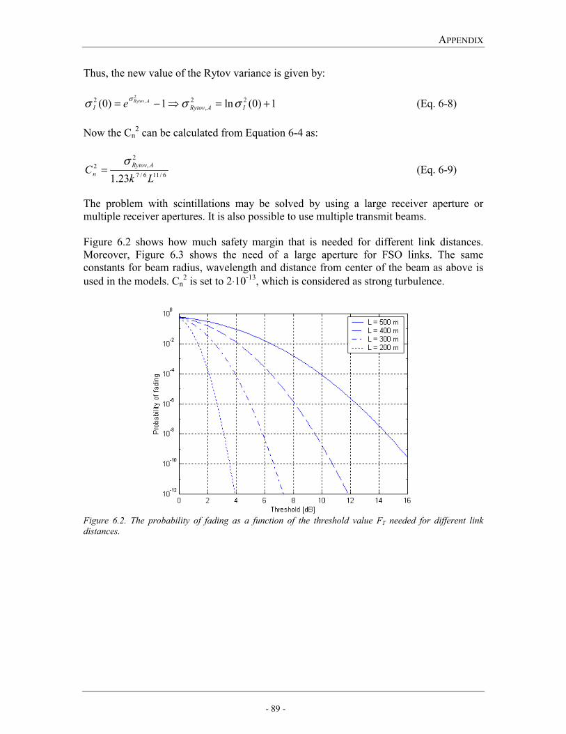
APPENDIX
- 89 -
Thus, the new value of the Rytov variance is given by:
1)0(ln1)0( 22,
2 2, +=−= IARytovIARytove σσσ σ (Eq. 6-8)
Now the Cn
2 can be calculated from Equation 6-4 as:
6/116/7
2,2
23.1 LkC ARytov
n
σ= (Eq. 6-9)
The problem with scintillations may be solved by using a large receiver aperture or multiple receiver apertures. It is also possible to use multiple transmit beams. Figure 6.2 shows how much safety margin that is needed for different link distances. Moreover, Figure 6.3 shows the need of a large aperture for FSO links. The same constants for beam radius, wavelength and distance from center of the beam as above is used in the models. Cn
2 is set to 2⋅10-13, which is considered as strong turbulence.
Figure 6.2. The probability of fading as a function of the threshold value FT needed for different link distances.
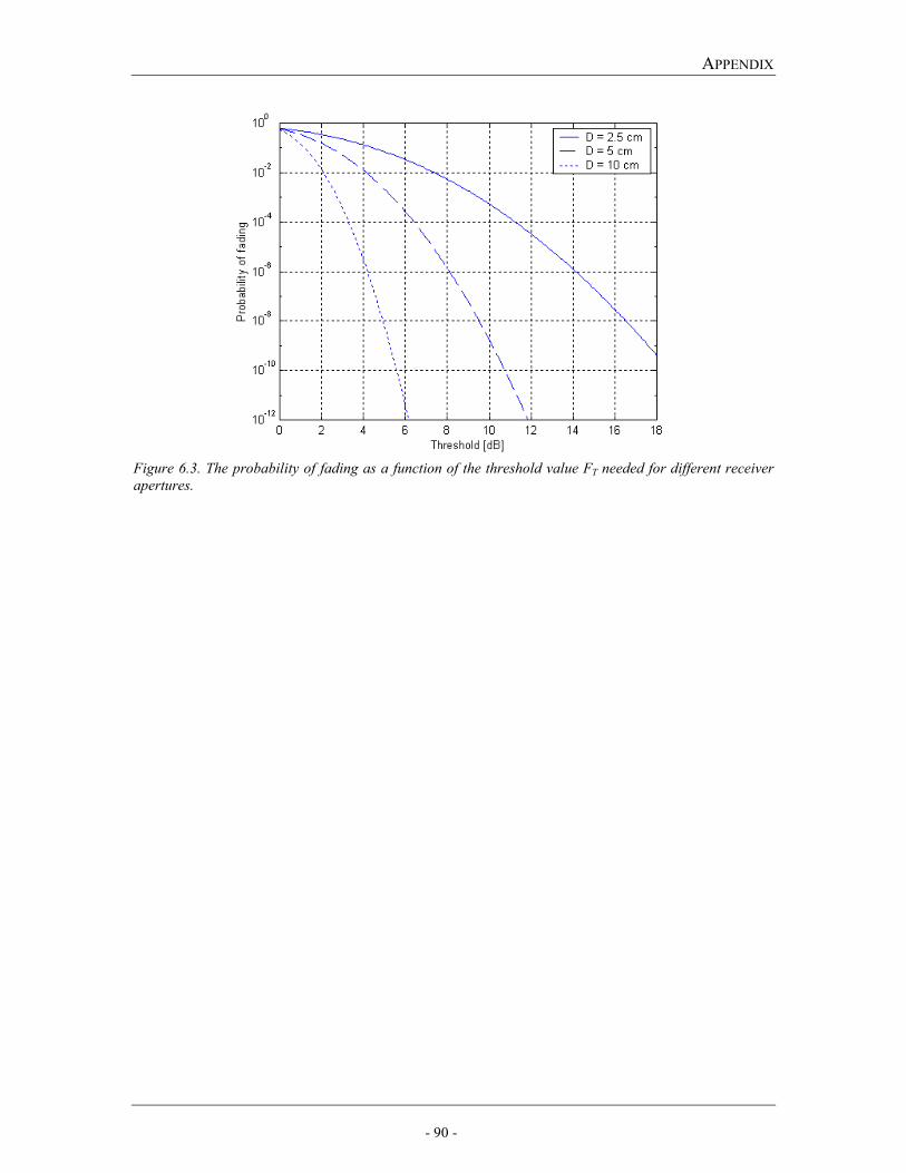
APPENDIX
- 90 -
Figure 6.3. The probability of fading as a function of the threshold value FT needed for different receiver apertures.