Embed Size (px)
Citation preview

Preliminary version of a paper to appear atElsevier Ad Hoc Networks Journal
Design and Analysis of a Propagation Delay TolerantALOHA Protocol for Underwater Networks
(Technical Report No.: ISI-2010-668)
Joon Ahna, Affan Syedb, Bhaskar Krishnamacharia, John Heidemannb
aMing Hsieh Department of Electrical EngineeringUniversity of Southern California, Los Angeles, CA 90089
bComputer Science Department and Information Sciences InstituteUniversity of Southern California, Los Angeles, CA 90089
Abstract
Acoustic underwater wireless sensor networks (UWSN) have recently gained at-tention as a topic of research. Such networks are characterized by increased uncer-tainty in medium access due not only to when data is sent, but also due to significantlydifferent propagation latencies from spatially diverse transmitters—together, we callthesespace-time uncertainty. We find that the throughput of slotted ALOHA degradesto pure ALOHA in such an environment with varying delay. We therefore proposehandling this spatial uncertainty by adding guard times to slotted ALOHA, formingPropagation Delay Tolerant (PDT-)ALOHA. We show that PDT-ALOHA increasesthroughput by 17–100% compared to simple slotted ALOHA in underwater settings.We analyze the protocol’s performance both mathematicallyand via extensive simu-lations. We find that the throughput capacity decreases as the maximum propagationdelay increases, and identify protocol parameter values that realize optimal throughput.Our results suggest that shorter hops improve throughput inUWSNs.
Keywords:Underwater Acoustic Network, ALOHA protocol, Medium Access Control Protocol,Performance Analysis, Optimization
1. Introduction
Underwater sensor networking (UWSN) is becoming an important area of research [1,2, 3]. Medium access control (MAC) in underwater networks has attracted strong atten-tion due to its potentially large impact to the overall network performance [4, 5, 6, 7].The most significant change from traditional radio-frequency (RF) networks to under-water acoustic networks is the change of themedium: acoustic instead of RF electro-magnetic waves. Latency and bandwidth have significant effects on control algorithms
Email addresses:[email protected] (Joon Ahn),[email protected] (Affan Syed),[email protected] (Bhaskar Krishnamachari),[email protected] (John Heidemann)
1

for MAC protocols. Both of these vary substantially in acoustic networks where prop-agation latencies are five-orders of magnitude greater thanRF, while bandwidths areone-thousandth that of RF.
ALOHA protocols have been the basis of many wireless MACs since their inven-tion in the 1970s [8]. They are the first class of contention-based MAC protocolsin a shared wireless medium. Later protocols, such as carrier sense multiple access(CSMA), achieve better performance than ALOHA in RF networks, due to their con-servative mechanism of “listening before transmitting” [9]. However, carrier sensebecomes very expensive in underwater acoustic networks dueto the large propagationdelay. The effect of the propagation delay on ALOHA protocols has been analyzed byKleinrock and Tobagi [9] showing that the protocols are not sensitive to the propaga-tion delay. However, their analysis does not consider the varying propagation delaysfrom different locations of nodes; thus its results do not completely hold for underwaternetworks.
The goal of this paper is to understand the impact of varying propagation latencyon medium access, with ALOHA protocols as a case study. First, we show thatthe location-dependent propagation latency has a fundamental impact on the slottedALOHA because, intuitively, a packet’s receive time at the receiver depends not onlyon its transmit time (time uncertainty) but also on its relative propagation delay to thereceiver (space uncertainty). We refer to this joint uncertainty asspace-time uncer-tainty. We show that both dimensions of uncertainty need to be handled at the sametime. Then, we propose the Propagation Delay Tolerant ALOHA(PDT-ALOHA) pro-tocol to improve the performance of the slotted ALOHA by adding guard times. Weexplore its performance through mathematical analysis andextensive simulations withan aim to discover the best operating parameters. We find that, in the high latency en-vironment of UWSN, throughput capacity (i.e. throughput optimized across all loads)of PDT-ALOHA improves by 17–100% compared to slotted ALOHA,depending onnetwork propagation delay. Our analysis show that the throughput can be kept within97% of optimal capacity of PDT-ALOHA with an additional slottime that is 69% ofthe maximum propagation delay, indicating that even with unknown or variable de-lay regime a pre-configured value of PDT-ALOHA is a substantial improvement onslotted ALOHA. We also find that the throughput capacity decreases with increasedpropagation delay, reinforcing the benefit of short-range,multi-hop communication inunderwater networks besides simply energy-efficient communication.
This paper combines and extends two previous published results [10, 11]. The firstof these prior works focused on protocol simulation [10], and the other on analysis [11];here we combine these results to both validate each against the other in common sce-narios, and to provide a definitive discussion of the conclusions. We therefore integraterelated work (Section 2) and align the metrics across the twopapers for consistent com-parison of experiments (Section 7). We confirm that both simulations and analysis areconsistent with each other. Finally in Section 7.4 we present a strong argument basedon results from ours and concomitant research that motivates short, multi-hop networksin an underwater acoustic environment
Our work is meant to explore intrinsic characteristics of the high latency acousticchannel in UWSN. Work on more sophisticated protocols than ALOHA is alreadyunderway for underwater networks, but we expect the evaluation and understanding
2
we develop here will support the ongoing development of new protocols.
2. Related Work
Recently there has been significant amount of work on designing and analyzingunderwater MAC protocols [4, 5, 12, 13, 14, 6, 7]. While this prior work develops newprotocols, here our goal is to understand the fundamental impact of space-time uncer-tainty in acoustic medium access and propose a framework foranalyzing the MAC per-formance. This understanding, however, suggests adding guard time to slotted ALOHAto improve its throughput underwater.
As for ALOHA protocols in underwater networks, Vieiraet al.[14] performed sim-ple analysis of slotted ALOHA and reached a conclusion similar to one of ours: slottedALOHA degrades to pure ALOHA under high latency. Xieet al. [6] have comparedthe performance of ALOHA and CSMA with RTS/CTS mechanism forunderwaternetworks. Gibsonet al. [7] have extended this work to analyze the performance ofALOHA in a linear multi-hop topology. These papers, howeverdo not attempt to ad-dress the following questions: why does pure ALOHA’s performance in underwaterremain the same as in RF? why does slotted ALOHA’s performance degrade to pureALOHA in the presence of varying propagation delay? How can this degradation behandled and what are the optimal parameters for it? In this paper we specifically ad-dress these questions and provide answers.
Theoretical work has begun to explore this direction. Vieira et al. [14] analyzedslotted ALOHA and concluded that it degrades to unslotted ALOHA under high prop-agation delay. Gibsonet al. [7] have analyzed the performance of ALOHA in a linearmulti-hop topology. However, these works do not consider the use of guard times torelieve the negative effect of the large propagation delay.
Adding guard time was previously considered in the design ofsloppy slotted ALOHA(SSA) [15]. But, SSA was designed for satellite networks with a single, centralized re-ceiver (the satellite). In such networks, they also have considered variable propagationdelay, but it’s assumed to be induced by the imperfection (or“sloppiness”) of eachnode’s implementation, not by the location ofeach node. In fact, nodes are located onthe ground, and so, approximately equidistant to the satellite resulting in similar prop-agation delay for each link. Our work, on the other hand, focuses on ad-hoc acousticsensor networks where the relative distance to the receivercan vary greatly from nodeto node.
3. Space-time Uncertainty and the ALOHA Protocol
In this section we summarize the concept of space-time uncertainty with regardsto medium access, first introduced in a prior work [12]. We then explore this con-cept in terms of the ALOHA protocol in a high-latency environment. This explorationprovides us with design guidelines for modifying ALOHA for an underwater MACprotocol which we then present in the next section.
3
(a) Same transmission time; nocollision at B
(b) Different transmission timebut collision at B
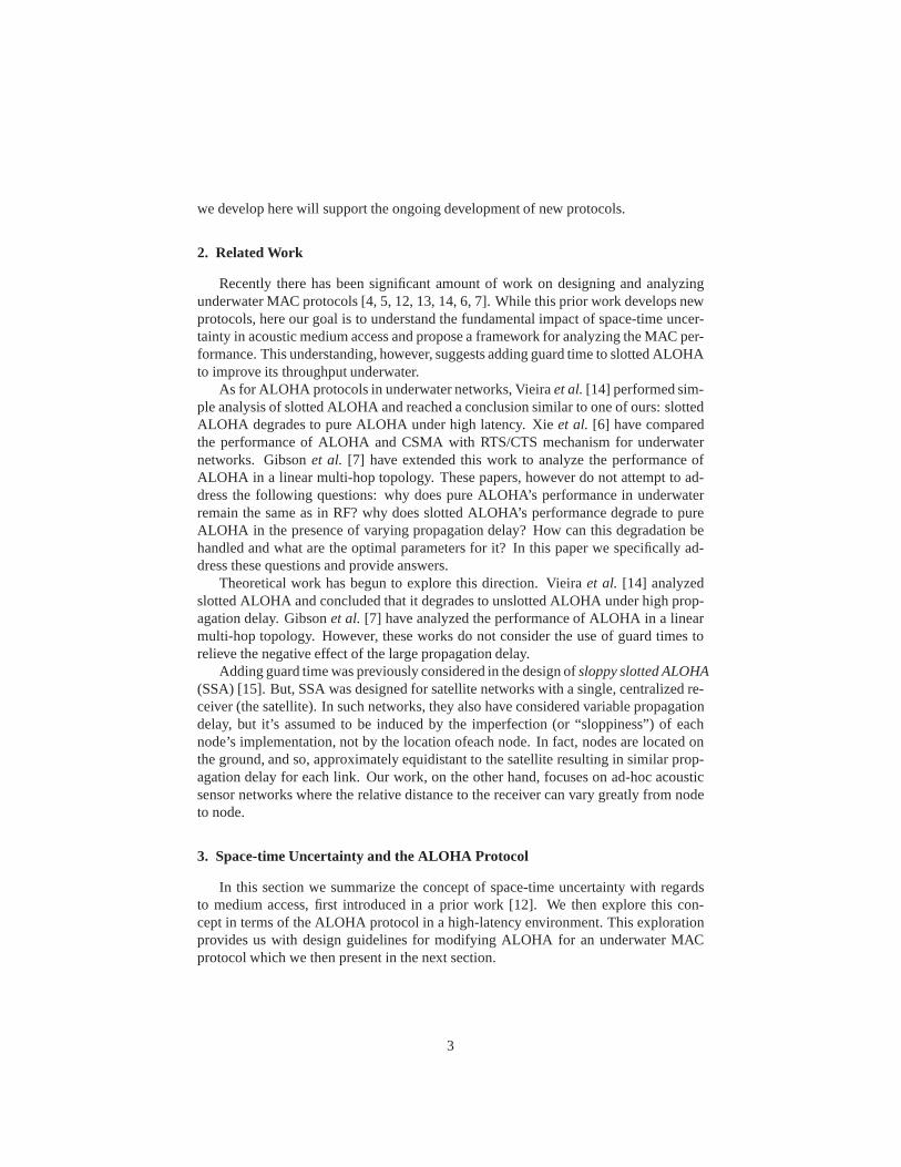
Figure 1: Illustration of space-time uncertainty
Vulnerability Interval
Data
2T
Time
T
(a) Aloha
Vulnerability Interval
Data
T
Time
T
Slot 0 Slot 1
(b) Slotted ALOHA
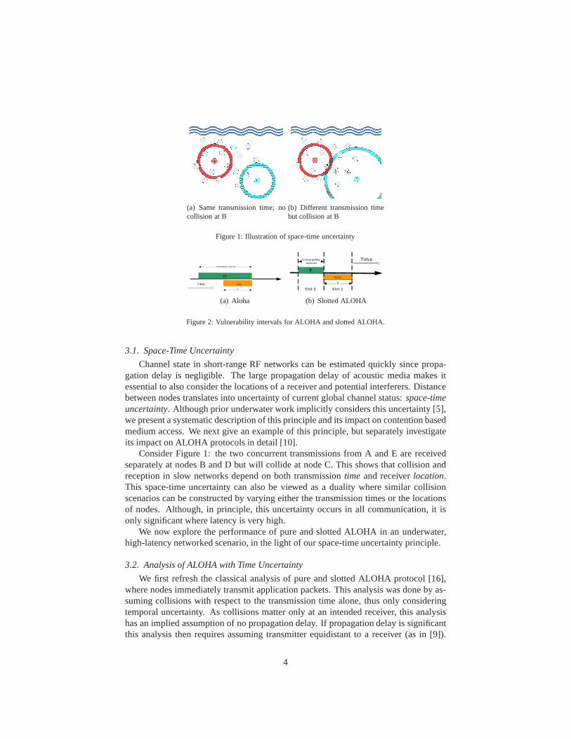
Figure 2: Vulnerability intervals for ALOHA and slotted ALOHA.
3.1. Space-Time Uncertainty
Channel state in short-range RF networks can be estimated quickly since propa-gation delay is negligible. The large propagation delay of acoustic media makes itessential to also consider the locations of a receiver and potential interferers. Distancebetween nodes translates into uncertainty of current global channel status:space-timeuncertainty. Although prior underwater work implicitly considers thisuncertainty [5],we present a systematic description of this principle and its impact on contention basedmedium access. We next give an example of this principle, butseparately investigateits impact on ALOHA protocols in detail [10].
Consider Figure 1: the two concurrent transmissions from A and E are receivedseparately at nodes B and D but will collide at node C. This shows that collision andreception in slow networks depend on both transmissiontime and receiverlocation.This space-time uncertainty can also be viewed as a duality where similar collisionscenarios can be constructed by varying either the transmission times or the locationsof nodes. Although, in principle, this uncertainty occurs in all communication, it isonly significant where latency is very high.
We now explore the performance of pure and slotted ALOHA in anunderwater,high-latency networked scenario, in the light of our space-time uncertainty principle.
3.2. Analysis of ALOHA with Time Uncertainty
We first refresh the classical analysis of pure and slotted ALOHA protocol [16],where nodes immediately transmit application packets. This analysis was done by as-suming collisions with respect to the transmission time alone, thus only consideringtemporal uncertainty. As collisions matter only at an intended receiver, this analysishas an implied assumption of no propagation delay. If propagation delay is significantthis analysis then requires assuming transmitter equidistant to a receiver (as in [9]).
4

0 0.5 1 1.5 2 2.5 30
0.05
0.1
0.15
0.2
0.25
0.3
0.35
0.4
0.45
Offered load
Nor
mal
ized
thro
ughp
ut
no delaya=0.01a=0.5a=1
(a) Pure ALOHA
0 0.5 1 1.5 2 2.5 30
0.05
0.1
0.15
0.2
0.25
0.3
0.35
0.4
0.45
Offered load
Nor
mal
ized
thro
ughp
ut
no delaya=0.01a=0.5a=1pure ALOHA (no delay)
(b) Slotted ALOHA
Figure 3: Throughput of pure and slotted ALOHA protocols vs.offered load (packets/transmission time);a is a parameter representing varying maximum propagations by normalizing the delay to the transmissiontime (more details in Section 5.1). This figure shows that forany valuea > 0, slotted ALOHA degrades topure ALOHA in underwater networks.
It further assumes an infinite numbers of nodes, with all arriving packets served at anew node and transmitted immediately into the network. The packets that collide arebuffered, making nodes backlogged. Such backlogged nodes retransmit after an expo-nential delay. The total offered load to the network is thus combination of the Poissonarrival and backlogged exponential retransmissions. Thisresults in a combined Pois-son packet arrival process (with meanλ) to the network having normalized throughputG(n) (expected packet/unit time) wheren represents the number of backlogged nodesin the network.
Thevulnerability interval (VI)is defined as thetime interval relative to a sender’stransmission within which another node’s transmission causes collision [9]. AssumingT as the packet transmission time, Figure 2(a) shows that the VI is equal to2T. On theother hand, slotted ALOHA allows transmission only at the start of synchronized slotsof lengthT . As Figure 2(b) shows, this synchronization ensures that only interferingpackets that arrive in slot 0 will result in a collision. It thus reduces the VI from2T toT by preventing any cross-slot overlap.
Classical analysis using the concept of vulnerability interval shows that slottedALOHA achieves maximum normalized throughput of1/e with λ of 1 packet per slot,while pure ALOHA achieves its maximum of1/2e at 0.5 packets/slot [16, 9].
As mentioned above, the classical analysis is carried out with respect to the trans-mitter’s time. The assumption of a single receiver equidistant to all transmitters resultsin a similar vulnerability interval at the receiver—regardless of the propagation delay(as shown by Klienrock and Tobagi [9]). Strictly speaking, these assumptions do nothold for all ad hoc wireless networks, but with short-range RF networks the variationin delay is small enough that it has virtually no effect on performance (for example,
5

Figure 4: Slotted transmission results in cross slots overlap at receiver.
Figure 5: Time diagram of packet transmission using PDT-ALOHA; A andB are transmitters andR is thereceiver.B locates closer to the receiver thanA.
10µs delay over 25m). In satellite networks delay is long, but there is typically onlyone sender or receiver. We next show, through simulation andanalysis, that the per-formance of ALOHA can be significantly affected in acoustic networks where theseassumptions do not hold.
3.3. ALOHA with Space Uncertainty
In order to understand the impact of location-dependent propagation latency, wenow simulate both simple ALOHA and slotted ALOHA with a event-based simulatordeveloped for underwater MAC research [12]. The simulationsetting is presented inSection 7.1. Our simulation results (Figure 3 and more details in [10]) showed twointeresting results.
First, throughput of pure ALOHA does not change, under any delay regime (Fig-ure 3(a)). This result is explained by looking at packet arrivals at thereceiver, with andwithout propagation delay. With no propagation delay the packet arrival at receiveris exactly the same as at transmitter. With propagation delay the arrival time at thereceiver is offset by a constant delay. Because the delay is constant for all packetssent by the transmitter, their arrivals at the receiver is still a Poisson process with thesame parameter as with no latency. Therefore, with the fact that the sum of indepen-dent Poisson processes is indeed a Poisson process, the throughput remains the samein either case. We should point out that pure ALOHA does not attempt to reduce timeuncertainty, hence further ignoring space uncertainty hasno impact.
The second interesting result is the degradation of slottedALOHA throughput tothat of pure ALOHA whenanypropagation latency is considered, shown by Figure 3(b)
6

(a similar observation was made by Vieiraet al. [14]). This is explained by lookingat the overlap of globally synchronized slots at a receiverR (Figure 4). Node A’stransmission in slot 1 can collide with any packet transmitted by node B in slot 1(queued at B in previous slot 0)andany one transmitted in slot 2 (queued during slot1).
Generalizing the above example, every transmitter has the collision with the pack-ets sent in the previous consecutive time slot from the transmitters located fartherfrom the receiver, in addition to the collision with the packets sent in the same timeslot. Also, every transmitter has another collision with the packets sent in the nextconsecutive time slot from the transmitters located nearerto the receiver. Hence,when transmitters are deployed uniformly at random in the area, a packet sent froman arbitrary transmitterni collides with a packet transmitted in the previous timeslot with probabilityp1 = (area farther thanni fromR)/(total area). With proba-bility p2 = (area nearer thanni fromR)/(total area), a packet sent from the trans-mitter collides with a packet transmitted in the next time slot. The probability thatthere is another transmitter with the same distance fromR is zero because its asso-ciated area is zero. And, we have a collision with probability 1 when more than onepacket is sent in the same time slot. Therefore, the expectedvulnerability interval isE[V I] = Tp1 + Tp2 + T = 2T sincep1 + p2 = 1. We use the expected VI becauseevery packet does not collide with every packet sent in the adjoining time slots.
This vulnerability interval is the same as in pure ALOHA, andthus any propagationlatency nullifies the benefit of time synchronization. If thenetwork always has a singlereceiver, and nodes knew their relative locations, it is conceivable for slotting to bemade relative to the receiver. However this simplification does not match the ad hocnetwork paradigm where any node can be a potential receiver.
Radio networks, although having very small propagation latency,doundergo a sim-ilar performance degradation, as we model any packet overlap as collision. However,most RF systems can usually tolerate an overlap of up to a single bit (depending oncoding techniques). As a result for high speed RF networks, if bit rate is 10Mb/s (e.g.,IEEE 802.11b), the maximum propagation delay that slotted ALOHA can tolerate is1ns, or 30m in distance. Thus such systems do not exhibit the immediate performancedegradation that we have shown for any propagation delay. Onthe other hand, acousticsystems even with low data rate modems (1Kb/s [17]) can tolerate only 1ms or 1.5min distance due to much slower speed of propagation (about 1500m/s). Thus, the im-pact of spatial uncertainty for slotted ALOHA will be more evident for any acousticnetwork than it is for RF networks.
4. PDT-ALOHA: the Protocol
We now postulate that space-time uncertainty can be handledby the addition ofextra guard time beyond the transmission time in time slots.These guard times areadded to ensure a single slot overlap at the receiver, thustoleratingthe large propaga-tion delays. We refer to this modified version as propagation-delay-tolerant ALOHA(PDT-ALOHA). As we argue in Section 3.3 while a centralized network can handlelarge delays by synchronizing slots at the receiver, a similar solution is not feasible forad-hoc networks where every node can be a potential receiver.
7

We first describe the modified protocol and the intuition on how guard time addstolerance to space-uncertainty. We then describe our methodology to evaluate the pro-tocol with both rigorous mathematical analysis and protocol simulations.
In our modification to slotted ALOHA, nodes still transmit only at the start of glob-ally synchronized slots. Global time synchronization can be achieved using underwatertime sync protocols such as [18, 19]. The slot duration, however, is increased fromTtoT +β ·τmax, whereβ represents the fraction of maximum propagation delay (τmax)that nodes wait after finishing their transmission (Figure 5). Hence,βτmax is the guardtime, andβ can be considered as thenormalized guard time. Choosingβ = 1 ensuresthat no overlap at the receiver occurs unless packets are transmitted in the same slot,the guarantee that slotted ALOHA was originally designed toachieve when delay isnot important. However this value ofβ results in a long wait time after each packetthat will increase packet transmission latency and bandwidth overhead. Withβ < 1there remains the possibility that some node pairs still have the vulnerability interval oftwo slot durations (as in Figure 4). Therefore, reducingβ value lowers the bandwidthoverhead, but increases collision probability. Based on the intuition that the distancebetween node pairs is often smaller than the maximum propagation delay, we varyβto evaluate the tradeoff between bandwidth overhead and collision probability.
5. Mathematical Analysis of PDT-ALOHA
In this section we analyze the performance of PDT-ALOHA. In particular, we in-vestigate key metrics including probability of collisions, success rate, and throughput.
5.1. Assumptions
We make the following assumptions to analyze the performance of the PDT-ALOHAprotocol below, unless stated otherwise.
We consider the one-hop ad-hoc underwater network where thenetwork has onereceiver and multiple transmitters. Because the network isad-hoc, the distance be-tween the receiver and transmitters are not necessarily equidistant. Hence, we assumethat the network has one receiver andn transmitters, which are deployed in the two-dimensional disk area. The receiver is located at the centerof the disk area, and thetransmitters are deployed uniformly at random in the area. We assume the 2D areabecause we consider the network deployed in the ocean floor.
The propagation speed of communication is a positive finite constant regardless ofthe location in the network, so that the maximum propagationtime τm is the propaga-tion time from the receiver to the farthest transmitter. Thetransmission rate is constantfor every transmitter. The packet size is constant so that the transmission time for apacket is constant, which we assume is one (without loss of generality). Only a properscaling is needed for some parameters, particularlyτm, in order to cope with the gen-eral transmission time. Hence, the normalized maximum propagation delaya to thetransmission time isa = τm/(transmission time) = τm.
We assume that the packet arrival per node at a given time slotfollows the I.I.D.Bernoulli distribution. Specifically, a transmitter sendsa packet to the receiver withprobabilityp in each time slot. Note that this provides discrete approximation to the
8
Poisson process of the packet arrivals to the network. If thereceiver receives more thanone packet simultaneously at any time in a time slot, all the packets involved fail toget delivered successfully causing a collision. The links over which transmissions takeplace are lossless. A transmitter always transmits a packetat the start of the time slotif the transmitter wants to send the packet. All the nodes have globally synchronizedtime slots. The transmission time is no less than the maximumpropagation time so thata ≤ 1.
The assumption thata ≤ 1 is to make sure that the collision between a time slotand another is confined to the consecutive time slots. So, with this assumption, there isno possibility that a packet sent ini-th time slot collides with another inj-th time slot,wherej /∈ {i− 1, i, i+ 1}.
5.2. Success Rate
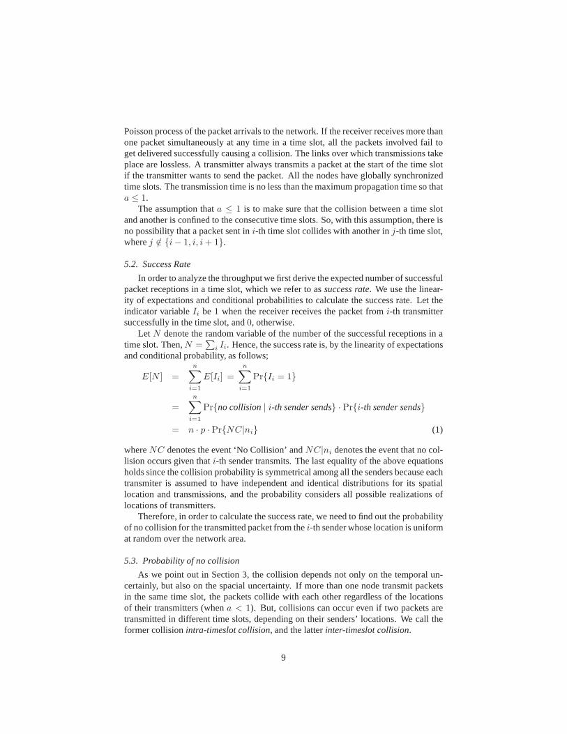
In order to analyze the throughput we first derive the expected number of successfulpacket receptions in a time slot, which we refer to assuccess rate. We use the linear-ity of expectations and conditional probabilities to calculate the success rate. Let theindicator variableIi be1 when the receiver receives the packet fromi-th transmittersuccessfully in the time slot, and0, otherwise.
Let N denote the random variable of the number of the successful receptions in atime slot. Then,N =
∑
i Ii. Hence, the success rate is, by the linearity of expectationsand conditional probability, as follows;
E[N ] =
n∑
i=1
E[Ii] =
n∑
i=1
Pr{Ii = 1}
=
n∑
i=1
Pr{no collision| i-th sender sends} · Pr{i-th sender sends}
= n · p · Pr{NC|ni} (1)
whereNC denotes the event ‘No Collision’ andNC|ni denotes the event that no col-lision occurs given thati-th sender transmits. The last equality of the above equationsholds since the collision probability is symmetrical amongall the senders because eachtransmiter is assumed to have independent and identical distributions for its spatiallocation and transmissions, and the probability considersall possible realizations oflocations of transmitters.
Therefore, in order to calculate the success rate, we need tofind out the probabilityof no collision for the transmitted packet from thei-th sender whose location is uniformat random over the network area.
5.3. Probability of no collision
As we point out in Section 3, the collision depends not only onthe temporal un-certainly, but also on the spacial uncertainty. If more thanone node transmit packetsin the same time slot, the packets collide with each other regardless of the locationsof their transmitters (whena < 1). But, collisions can occur even if two packets aretransmitted in different time slots, depending on their senders’ locations. We call theformer collisionintra-timeslot collision, and the latterinter-timeslot collision.
9
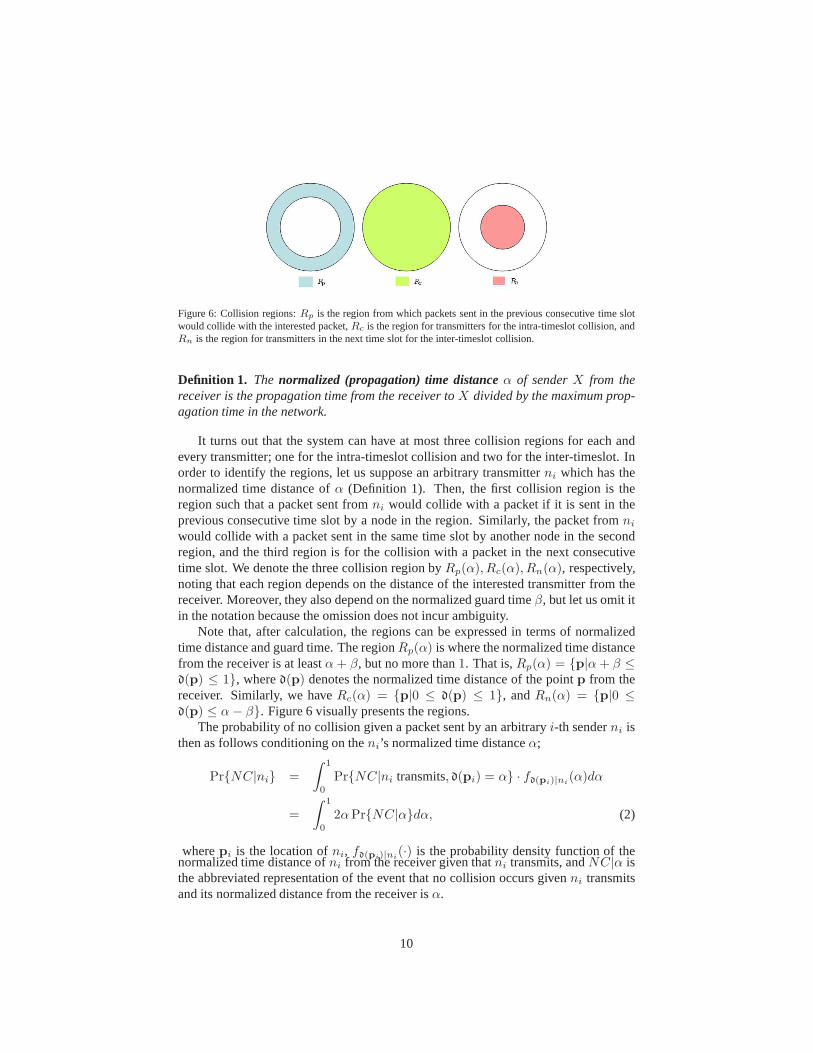
Figure 6: Collision regions:Rp is the region from which packets sent in the previous consecutive time slotwould collide with the interested packet,Rc is the region for transmitters for the intra-timeslot collision, andRn is the region for transmitters in the next time slot for the inter-timeslot collision.
Definition 1. The normalized (propagation) time distance α of senderX from thereceiver is the propagation time from the receiver toX divided by the maximum prop-agation time in the network.
It turns out that the system can have at most three collision regions for each andevery transmitter; one for the intra-timeslot collision and two for the inter-timeslot. Inorder to identify the regions, let us suppose an arbitrary transmitterni which has thenormalized time distance ofα (Definition 1). Then, the first collision region is theregion such that a packet sent fromni would collide with a packet if it is sent in theprevious consecutive time slot by a node in the region. Similarly, the packet fromni
would collide with a packet sent in the same time slot by another node in the secondregion, and the third region is for the collision with a packet in the next consecutivetime slot. We denote the three collision region byRp(α), Rc(α), Rn(α), respectively,noting that each region depends on the distance of the interested transmitter from thereceiver. Moreover, they also depend on the normalized guard timeβ, but let us omit itin the notation because the omission does not incur ambiguity.
Note that, after calculation, the regions can be expressed in terms of normalizedtime distance and guard time. The regionRp(α) is where the normalized time distancefrom the receiver is at leastα+ β, but no more than1. That is,Rp(α) = {p|α+ β ≤d(p) ≤ 1}, whered(p) denotes the normalized time distance of the pointp from thereceiver. Similarly, we haveRc(α) = {p|0 ≤ d(p) ≤ 1}, andRn(α) = {p|0 ≤d(p) ≤ α− β}. Figure 6 visually presents the regions.
The probability of no collision given a packet sent by an arbitrary i-th senderni isthen as follows conditioning on theni’s normalized time distanceα;
Pr{NC|ni} =
∫ 1
0
Pr{NC|ni transmits, d(pi) = α} · fd(pi)|ni(α)dα
=
∫ 1
0
2αPr{NC|α}dα, (2)
wherepi is the location ofni, fd(pi)|ni(·) is the probability density function of the
normalized time distance ofni from the receiver given thatni transmits, andNC|α isthe abbreviated representation of the event that no collision occurs givenni transmitsand its normalized distance from the receiver isα.
10
The last equation holds because the location of a node is independent of the packettransmission and the transmitters are deployed uniformly in our assumption.
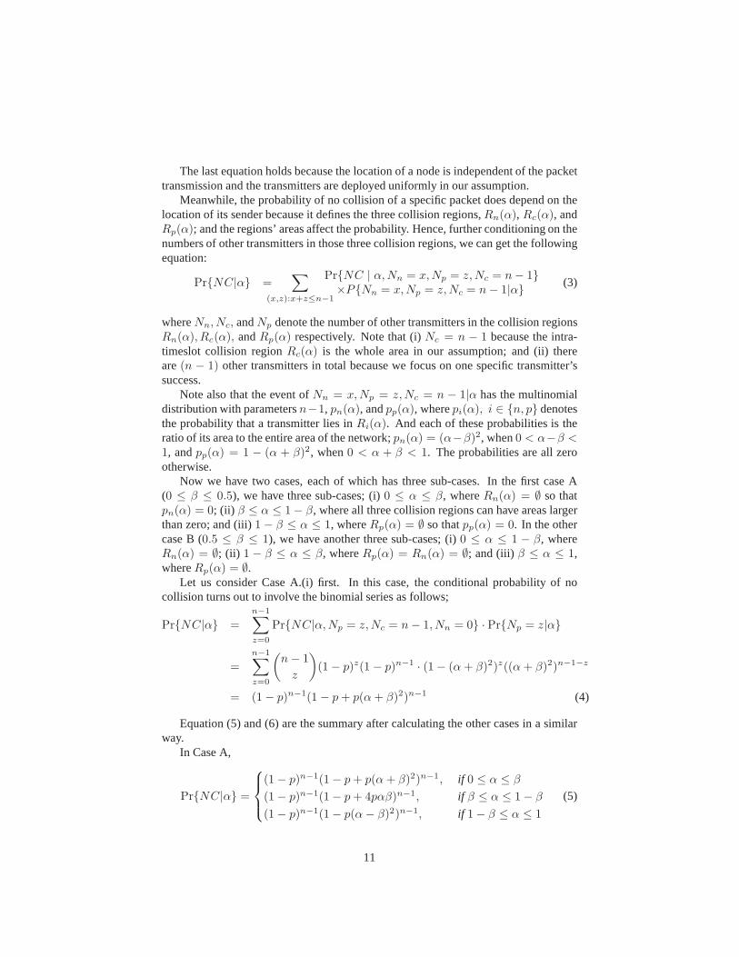
Meanwhile, the probability of no collision of a specific packet does depend on thelocation of its sender because it defines the three collisionregions,Rn(α), Rc(α), andRp(α); and the regions’ areas affect the probability. Hence, further conditioning on thenumbers of other transmitters in those three collision regions, we can get the followingequation:
Pr{NC|α} =∑
(x,z):x+z≤n−1
Pr{NC | α,Nn = x,Np = z,Nc = n− 1}×P{Nn = x,Np = z,Nc = n− 1|α}
(3)
whereNn, Nc, andNp denote the number of other transmitters in the collision regionsRn(α), Rc(α), andRp(α) respectively. Note that (i)Nc = n − 1 because the intra-timeslot collision regionRc(α) is the whole area in our assumption; and (ii) thereare(n − 1) other transmitters in total because we focus on one specific transmitter’ssuccess.
Note also that the event ofNn = x,Np = z,Nc = n − 1|α has the multinomialdistribution with parametersn−1, pn(α), andpp(α), wherepi(α), i ∈ {n, p} denotesthe probability that a transmitter lies inRi(α). And each of these probabilities is theratio of its area to the entire area of the network;pn(α) = (α−β)2, when0 < α−β <1, andpp(α) = 1 − (α + β)2, when0 < α + β < 1. The probabilities are all zerootherwise.
Now we have two cases, each of which has three sub-cases. In the first case A(0 ≤ β ≤ 0.5), we have three sub-cases; (i)0 ≤ α ≤ β, whereRn(α) = ∅ so thatpn(α) = 0; (ii) β ≤ α ≤ 1− β, where all three collision regions can have areas largerthan zero; and (iii)1 − β ≤ α ≤ 1, whereRp(α) = ∅ so thatpp(α) = 0. In the othercase B (0.5 ≤ β ≤ 1), we have another three sub-cases; (i)0 ≤ α ≤ 1 − β, whereRn(α) = ∅; (ii) 1 − β ≤ α ≤ β, whereRp(α) = Rn(α) = ∅; and (iii) β ≤ α ≤ 1,whereRp(α) = ∅.
Let us consider Case A.(i) first. In this case, the conditional probability of nocollision turns out to involve the binomial series as follows;
Pr{NC|α} =
n−1∑
z=0
Pr{NC|α,Np = z,Nc = n− 1, Nn = 0} · Pr{Np = z|α}
=
n−1∑
z=0
(
n− 1
z
)
(1− p)z(1 − p)n−1 · (1− (α+ β)2)z((α+ β)2)n−1−z
= (1− p)n−1(1 − p+ p(α+ β)2)n−1 (4)
Equation (5) and (6) are the summary after calculating the other cases in a similarway.
In Case A,
Pr{NC|α} =
(1− p)n−1(1− p+ p(α+ β)2)n−1, if 0 ≤ α ≤ β
(1− p)n−1(1− p+ 4pαβ)n−1, if β ≤ α ≤ 1− β
(1− p)n−1(1− p(α− β)2)n−1, if 1− β ≤ α ≤ 1
(5)
11

In Case B,
Pr{NC|α} =
(1− p)n−1(1− p+ p(α+ β)2)n−1, if 0 ≤ α ≤ 1− β
(1− p)n−1, if 1− β ≤ α ≤ β
(1− p)n−1(1− p(α− β)2)n−1, if β ≤ α ≤ 1
(6)
Substituting (5) or (6) into (2) we can obtain the expressionfor the probability ofno collision which can be evaluated easily with the numerical method.
Note that the expression for probability of no collision does not involve the maxi-mum propagation delayτm implying the probability is independent ofτm so that thesuccess rate is also independent ofτm. It turns out from Theorem 1 that the success rateis independent ofτm even after relaxing the assumption of 2D unit disk of the networkand the identical distribution of packet transmission for each node.
Theorem 1. Suppose a network of nodes with fixed spatial locations of nodes, a fixedtransmission probabilitypi in a time slot for each nodei, and a transmission timeTfor a packet. Then, the success ratef is independent of the maximum propagation timeτm in the network as long as0 < τm ≤ T . In other words, it is independent of thepropagation speedvp.
PROOF. Since the spatial locations of nodes are fixed, the spatial distancerm from thereceiver to the farthest node is constant;rm = τm · vp = const.
The spatial distanceri of an arbitraryi-th transmitter is also fixed, and so the nor-malized propagation time delayαi of the node is constant regardless ofrm as long asrm > 0 or 0 < vp < ∞ because of the following:
ri = αi · τm · vp = αi · rm ⇒ αi =rirm
= const.
Let r(Ri) denote the spatial region associate with the collision regionRi. Then,the spatial region ofRn, Rc, andRp are all fixed regardless ofτm because
r(Rn) = {r : 0 ≤ r ≤ (αi − β)τmvp = (αi − β)rm}
r(Rc) = {r : 0 ≤ r ≤ τmvp = rm}
r(Rp) = {r : (αi + β)rm ≤ r ≤ rm}
andαi, β, andrm are all constants.Hence, the number of nodes in each ofRn, Rc, andRp is constant regardless of
the speed of propagation, and so the probability of no collision of thei-th transmitteris constant. Therefore,
f =∑
i
pi Pr{NC|ni} = const. with respect toτm�
5.4. Throughput for finite number of nodesIn this paper we consider the throughputS in packets per transmission time. Be-
cause the size of time slot is1 + βa, S can be expressed as follows:
S(n, β, p, a) =f(n, β, p)
1 + βa=
npPr{NC|ni}
1 + βa(7)
12
limn→∞
(
1−
λ
n
)n−1
= e−λ
limn→∞
(
1−
λ
n+
λ
n(α+ β)2
)n−1
= e−λ+λ(α+β)2
limn→∞
(
1−
λ
n+ 4
λ
nαβ
)n−1
= e−λ+4λαβ
limn→∞
(
1−
λ
n(α− β)2
)n−1
= e−λ(α−β)2
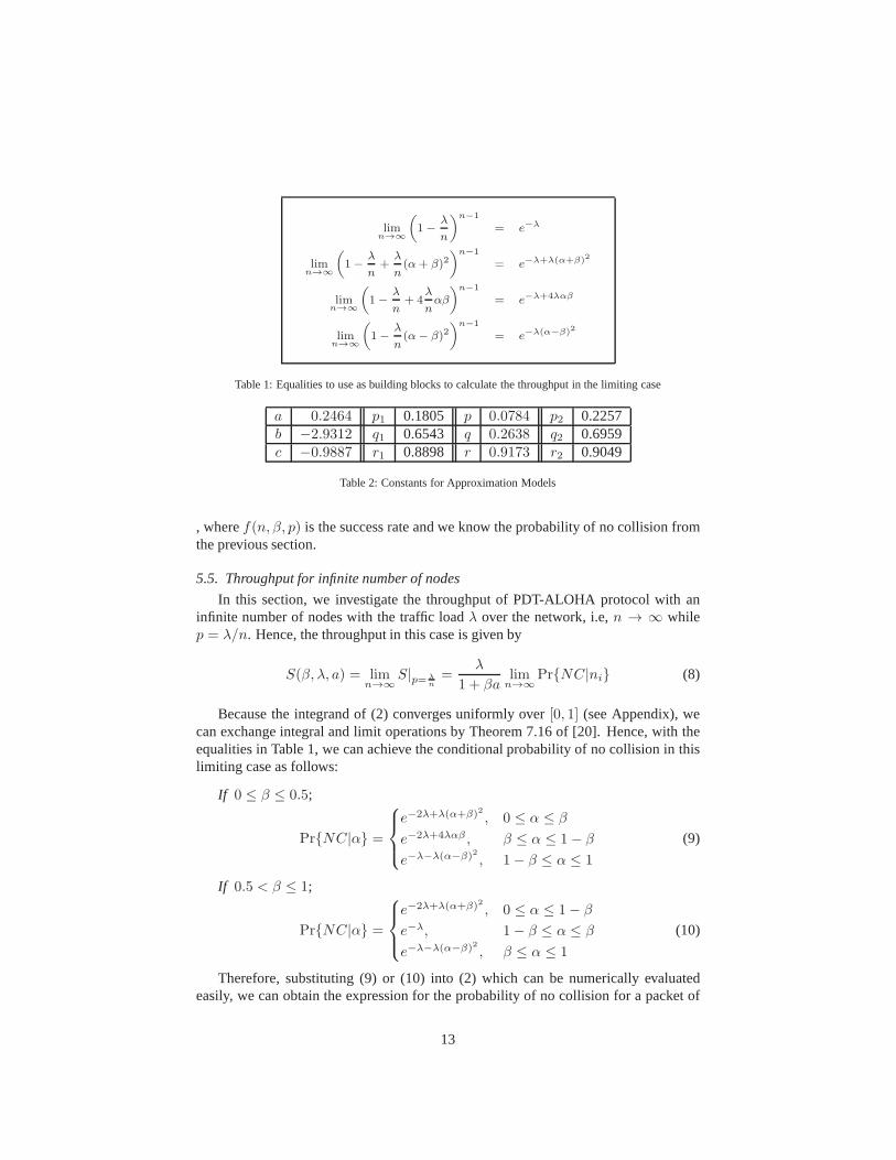
Table 1: Equalities to use as building blocks to calculate the throughput in the limiting case
a 0.2464 p1 0.1805 p 0.0784 p2 0.2257b −2.9312 q1 0.6543 q 0.2638 q2 0.6959c −0.9887 r1 0.8898 r 0.9173 r2 0.9049
Table 2: Constants for Approximation Models
, wheref(n, β, p) is the success rate and we know the probability of no collision fromthe previous section.
5.5. Throughput for infinite number of nodes
In this section, we investigate the throughput of PDT-ALOHAprotocol with aninfinite number of nodes with the traffic loadλ over the network, i.e,n → ∞ whilep = λ/n. Hence, the throughput in this case is given by
S(β, λ, a) = limn→∞
S|p=λ
n
=λ
1 + βalimn→∞
Pr{NC|ni} (8)
Because the integrand of (2) converges uniformly over[0, 1] (see Appendix), wecan exchange integral and limit operations by Theorem 7.16 of [20]. Hence, with theequalities in Table 1, we can achieve the conditional probability of no collision in thislimiting case as follows:
If 0 ≤ β ≤ 0.5;
Pr{NC|α} =
e−2λ+λ(α+β)2 , 0 ≤ α ≤ β
e−2λ+4λαβ , β ≤ α ≤ 1− β
e−λ−λ(α−β)2 , 1− β ≤ α ≤ 1
(9)
If 0.5 < β ≤ 1;
Pr{NC|α} =
e−2λ+λ(α+β)2 , 0 ≤ α ≤ 1− β
e−λ, 1− β ≤ α ≤ β
e−λ−λ(α−β)2 , β ≤ α ≤ 1
(10)
Therefore, substituting (9) or (10) into (2) which can be numerically evaluatedeasily, we can obtain the expression for the probability of no collision for a packet of
13
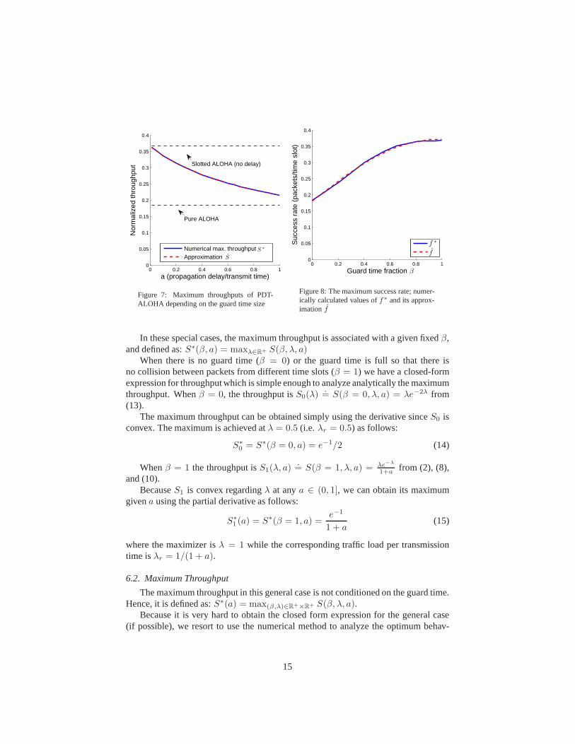
a transmitter. We shall use numerical evaluations to investigate the properties of themaximum throughput and obtain a very simple approximation for it in Section 6.2.
5.6. Throughput with no guard time
We derive the throughput of PDT-ALOHA for the case where there is no guardtime (i.e. β = 0) and the number of nodes is infinite, using our derivation forthegeneral case developed in previous sections. We present this as a sanity check becausewe know that, without the guard time, the PDT-ALOHA is equivalent to the traditionalslotted ALOHA, whose performace degrades to that of the pure(unslotted) ALOHAgiven by (as discussed in Section 3.3)
Thpure = λe−2λ (11)
For our derivation, no guard time (β = 0) impliesPr{NC|α} = e−2λ from (9),which in turn impies from (2)
Pr{NC|ni} =
∫ 1
0
2αe−2λdα = e−2λ (12)
Therefore, the throughput of PDT-ALOHA is given from (8) by
S(β = 0, λ, a) = λe−2λ (13)
This shows our derivation correctly capture the throughputmechanism for the no-gaurd-time case and the phenomenon that the amount of maximum propagation timebecomes irrelevant to the throughput when there is no guard time for PDT-ALOHA.
6. Optimization of PDT-ALOHA
In this section we investigate themaximumsuccess rate and themaximumthrough-put of PDT-ALOHA protocol. We also have an interest in the protocol parameters,particularly the size of guard time and the traffic load, which realize the maximumthroughput.
We consider the traffic load per transmission timeλr as well as the load per timeslot λ because it is useful to compare traffic loads between systemsof different sizeof time slot. And, it turns out it gives simpler approximation for the optimum values.These two kinds of traffic load have the relationship asλr = λ/(1 + βa).
Although we assume in this section the limiting case, where the number of nodesin the network is infinite, it is fairly straightforward to adapt the method we used herefor the finite number of nodes.
6.1. Special Cases
We start with special cases, i.e.β = 0, or β = 1, which can be analyzed analyti-cally. Then, we examine general cases given a network size interms of the maximumpropagation delay in Section 6.2.
14
0 0.2 0.4 0.6 0.8 10
0.05
0.1
0.15
0.2
0.25
0.3
0.35
0.4
a (propagation delay/transmit time)
Nor
mal
ized
thro
ughp
ut
Numerical max. throughputApproximation
Slotted ALOHA (no delay)
Pure ALOHA
S ∗
S
Figure 7: Maximum throughputs of PDT-ALOHA depending on the guard time size
0 0.2 0.4 0.6 0.8 10
0.05
0.1
0.15
0.2
0.25
0.3
0.35
0.4
Guard time fraction
Suc
cess
rat
e (p
acke
ts/ti
me
slot
)
f ∗
f
β
Figure 8: The maximum success rate; numer-ically calculated values off∗ and its approx-imation f
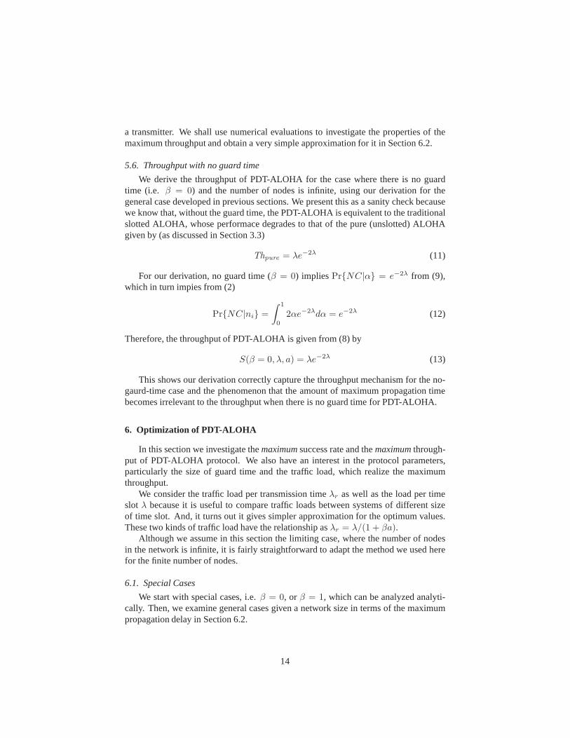
In these special cases, the maximum throughput is associated with a given fixedβ,and defined as:S∗(β, a) = maxλ∈R+ S(β, λ, a)
When there is no guard time (β = 0) or the guard time is full so that there isno collision between packets from different time slots (β = 1) we have a closed-formexpression for throughput which is simple enough to analyzeanalytically the maximumthroughput. Whenβ = 0, the throughput isS0(λ)
.= S(β = 0, λ, a) = λe−2λ from
(13).The maximum throughput can be obtained simply using the derivative sinceS0 is
convex. The maximum is achieved atλ = 0.5 (i.e. λr = 0.5) as follows:
S∗0 = S∗(β = 0, a) = e−1/2 (14)
Whenβ = 1 the throughput isS1(λ, a).= S(β = 1, λ, a) = λe−λ
1+afrom (2), (8),
and (10).BecauseS1 is convex regardingλ at anya ∈ (0, 1], we can obtain its maximum
givena using the partial derivative as follows:
S∗1 (a) = S∗(β = 1, a) =
e−1
1 + a(15)
where the maximizer isλ = 1 while the corresponding traffic load per transmissiontime isλr = 1/(1 + a).
6.2. Maximum Throughput
The maximum throughput in this general case is not conditioned on the guard time.Hence, it is defined as:S∗(a) = max(β,λ)∈R+×R+ S(β, λ, a).
Because it is very hard to obtain the closed form expression for the general case(if possible), we resort to use the numerical method to analyze the optimum behav-
15
ior of the system. Based on the result of the numerical analysis, we propose simpleapproximations for the optimum behavior and its protocol parameters.
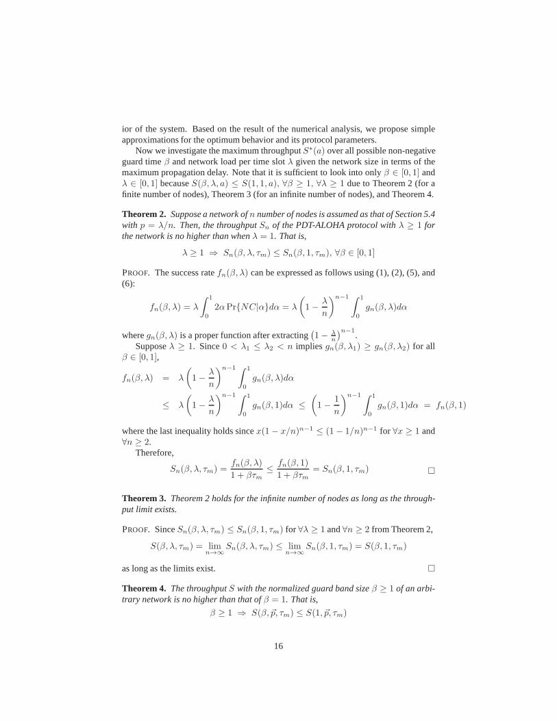
Now we investigate the maximum throughputS∗(a) over all possible non-negativeguard timeβ and network load per time slotλ given the network size in terms of themaximum propagation delay. Note that it is sufficient to lookinto onlyβ ∈ [0, 1] andλ ∈ [0, 1] becauseS(β, λ, a) ≤ S(1, 1, a), ∀β ≥ 1, ∀λ ≥ 1 due to Theorem 2 (for afinite number of nodes), Theorem 3 (for an infinite number of nodes), and Theorem 4.
Theorem 2. Suppose a network ofn number of nodes is assumed as that of Section 5.4with p = λ/n. Then, the throughputSn of the PDT-ALOHA protocol withλ ≥ 1 forthe network is no higher than whenλ = 1. That is,
λ ≥ 1 ⇒ Sn(β, λ, τm) ≤ Sn(β, 1, τm), ∀β ∈ [0, 1]
PROOF. The success ratefn(β, λ) can be expressed as follows using (1), (2), (5), and(6):
fn(β, λ) = λ
∫ 1
0
2αPr{NC|α}dα = λ
(
1−λ
n
)n−1 ∫ 1
0
gn(β, λ)dα
wheregn(β, λ) is a proper function after extracting(
1− λn
)n−1.
Supposeλ ≥ 1. Since0 < λ1 ≤ λ2 < n impliesgn(β, λ1) ≥ gn(β, λ2) for allβ ∈ [0, 1],
fn(β, λ) = λ
(
1−λ
n
)n−1 ∫ 1
0
gn(β, λ)dα
≤ λ
(
1−λ
n
)n−1 ∫ 1
0
gn(β, 1)dα ≤
(
1−1
n
)n−1 ∫ 1
0
gn(β, 1)dα = fn(β, 1)
where the last inequality holds sincex(1 − x/n)n−1 ≤ (1 − 1/n)n−1 for ∀x ≥ 1 and∀n ≥ 2.
Therefore,
Sn(β, λ, τm) =fn(β, λ)
1 + βτm≤
fn(β, 1)
1 + βτm= Sn(β, 1, τm) �
Theorem 3. Theorem 2 holds for the infinite number of nodes as long as the through-put limit exists.
PROOF. SinceSn(β, λ, τm) ≤ Sn(β, 1, τm) for ∀λ ≥ 1 and∀n ≥ 2 from Theorem 2,
S(β, λ, τm) = limn→∞
Sn(β, λ, τm) ≤ limn→∞
Sn(β, 1, τm) = S(β, 1, τm)
as long as the limits exist. �
Theorem 4. The throughputS with the normalized guard band sizeβ ≥ 1 of an arbi-trary network is no higher than that ofβ = 1. That is,
β ≥ 1 ⇒ S(β, ~p, τm) ≤ S(1, ~p, τm)
16

PROOF. If β ≥ 1, there is no longer collision of packets between different time slotsandβ does not have any effect on packets sent in the same time slot.Hence, the successrate is same forβ ≥ 1 as that ofβ = 1. However, increasingβ makes the size of timeslot increases. Therefore, the claim follows. �
We evaluate the maximum throughputS∗ for 21 values ofτm starting from 0.01 to1 using the numerical method. After examining the behavior of S∗, we have found outthat the following simple expression can approximateS∗ quite closely:
S(a) = p+q
a+ r(16)
wherep, q, andr are constants. The curve-fitted values for the constants arepresentedin Table 2.
Figure 7 shows the accuracy of the approximation; The plot for S∗ is the inter-polation of 21 data points of the maximum throughput over offered loads and guardtimes found by numerical methods. As can be seen, our approximation has reasonablygood accuracy. Quantitatively, it does not deviate more than 0.3% from the numericalevaluations ofS∗.
The optimum values of protocol parameters which realize theoptimum throughputare also of interest. In particular, we are interested in theoptimum size of the guardtimeβ∗ and the optimum traffic loadλ∗
r per transmission time given the network sizein terms ofa. Through the numerical analysis we have found out that the optimizerβ∗
andλ∗r can be closely approximated with the following models:
β(a) = p1 +q1
a+ r1(17)
λr(a) = p2 +q2
a+ r2(18)
wherepi, qi, andri, ∀i ∈ {1, 2} are constants; their proper values are given in Table 2through curve fitting.
Figure 9 pictorially presents optimizersβ∗ andλ∗r , and their approximations de-
pending on the maximum propagation delaya. It also shows the guard timeβa nor-malized to the transmission time, which is one in our paper. As can be seen, our ap-proximations are very close to their numerical counterparts, respectively;β deviates nomore than 2% whileλr differs no more than 0.2%. We can also see that the optimumguard time is less than roughly half of the transmission time, and it is monotonicallyincreasing as the maximum propagation delay increases.
6.3. Maximum success rate
In this subsection we consider the maximum success rate. We first present the an-alytic findings about the properties of the maximum number ofsuccessful receptions.The findings are more general than what we assume previously.We find out throughTheorem 6 that, as long as the maximum propagation delay is less than the transmis-sion time of a packet, the maximum success rate is monotonically non-decreasing withrespect to the guard timeβ even when the network area is no longer 2D disk and thesending probability is not identical for each node.
17
0 0.2 0.4 0.6 0.8 10.5
0.55
0.6
0.65
0.7
0.75
0.8
0.85
0.9
a
Gua
rd ti
me
frac
tion
β
β ∗
β
(a)
0 0.2 0.4 0.6 0.8 10
0.1
0.2
0.3
0.4
0.5
a
Gua
rd ti
me
β a
β ∗a
βa
(b)
0 0.2 0.4 0.6 0.8 10.55
0.6
0.65
0.7
0.75
0.8
0.85
0.9
0.95
1
a
Offe
red
load
(pa
cket
s/tr
ansm
it tim
e)
λ∗
r
λr
(c)
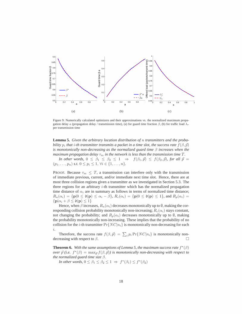
Figure 9: Numerically calculated optimizers and their approximations vs. the normalized maximum propa-gation delaya (propagation delay / transmission time), (a) for guard timefractionβ, (b) for traffic loadλr
per transmission time
Lemma 5. Given the arbitrary location distribution ofn transmitters and the proba-bility pi that i-th transmitter transmits a packet in a time slot, the success ratef(β, ~p)is monotonically non-decreasing as the normalized guard timeβ increases when themaximum propagation delayτm in the network is less than the transmission timeT .
In other words,0 ≤ β1 ≤ β2 ≤ 1 ⇒ f(β1, ~p) ≤ f(β2, ~p), for all ~p =(p1, . . . , pn) s.t.0 ≤ pi ≤ 1, ∀i ∈ {1, . . . , n}.
PROOF. Becauseτm ≤ T , a transmission can interfere only with the transmissionof immediate previous, current, and/or immediate next timeslot. Hence, there are atmost three collision regions given a transmitter as we investigated in Section 5.3. Thethree regions for an arbitraryi-th transmitter which has the normalized propagationtime distance ofαi are in summary as follows in terms of normalized time distance;Rn(αi) = {p|0 ≤ d(p) ≤ αi − β}, Rc(αi) = {p|0 ≤ d(p) ≤ 1}, andRp(αi) ={p|αi + β ≤ d(p) ≤ 1}
Hence, whenβ increases,Rn(αi) decreases monotonically up to∅, making the cor-responding collision probability monotonically non-increasing;Rc(αi) stays constant,not changing the probability; andRp(αi) decreases monotonically up to∅, makingthe probability monotonically non-increasing. These implies that the probability of nocollision for thei-th transmitterPr{NC|ni} is monotonically non-decreasing for eachi.
Therefore, the success ratef(β, ~p) =∑
i pi Pr{NC|ni} is monotonically non-decreasing with respect toβ. �
Theorem 6. With the same assumptions of Lemma 5, the maximum success ratef∗(β)over~p (i.e. f∗(β) = max~p f(β, ~p)) is monotonically non-decreasing with respect tothe normalized guard time sizeβ.
In other words,0 ≤ β1 ≤ β2 ≤ 1 ⇒ f∗(β1) ≤ f∗(β2)
18

PROOF. From the definition off∗ and Lemma 5,
f∗(β2) ≥ f(β2, ~p) ≥ f(β1, ~p), ∀~p
Therefore,f∗(β2) is an upper bound off(β1, ~p) for all ~p, which implies the fol-lowing:
f∗(β2) ≥ max~p
f(β1, ~p) = f∗(β1) �
As in the previous subsection, we use the numerical method toevaluatef∗. Theblack solid line of Figure 8 shows the interpolation of 22 data points off∗ foundnumerically.
Although it is hard to obtain the exact expression off∗, we know from Theorem 6that the maximized functionf∗(β) = maxλ f(β, λ) is monotonically non-decreasing.From this fact and the observation that the log-scale plot ofthe numerically evaluatedf∗(β) is approximately of cubic function, we are able to propose the following approx-imation model forf∗(β):
f(β) = ea(β−1)2(β+b)+c (19)
wherea, b, andc are constants and the constraint thatb < −1 makes sure that thefunction is monotonically increasing.
The red dashed line of Figure 8 shows this approximation withproper constantssuggested in Table 2, as determined through numerical curvefitting.
7. Analysis and Comparison with Protocol Simulation
We now analyze the results of optimal throughput of PDT-ALOHA obtained inprevious section to observe the effect of guard time and network delay regime. Fur-thermore, for comparison we simulate PDT-ALOHA to verify the correctness of ouranalysis in a realistic network. We first introduce the parameters of the simulation usedfor comparison and then focus on the results. We end this section by drawing someinteresting conclusions from these results.
7.1. Simulation Parameters and Assumptions
We run our simulations using a custom-built, packet-level simulator designed forUWSN MAC research [12]1. Our simulation scenario consists of a single receiver thatdoes not transmit, with nodes randomly deployed in a circular region with a radiusequal to the maximum propagation delay. Nodes, with a singlepacket buffer, trans-mit based on an offered load to the network modeled as a Poisson process, with meanranging from 0 to 3 packets/transmission time, and we only observe the packets suc-cessfully received at our designated receiver. We choose a single receiver to parallelour analysis of protocol behavior, but have verified that ourresults hold with packetsreception at other nodes in the network. Protocol performance is evaluated through
1This simulator is available from the authors athttp://www.isi.edu/ilense/software/.
19

0 0.2 0.4 0.6 0.8 10
0.05
0.1
0.15
0.2
0.25
0.3
0.35
0.4
Guard band fraction β
Nor
mal
ized
thro
ughp
ut
Slotted ALOHA (no delay)a=0.01 a=0.1a=0.5
a=1
Pure ALOHA
(a) Analytical result
0 0.2 0.4 0.6 0.8 10
0.05
0.1
0.15
0.2
0.25
0.3
0.35
0.4
Guard band fraction β
Nor
mal
ized
Thr
ough
put
Slotted ALOHA (no delay)
a=0.01a=0.1a=0.5
a=1
Pure ALOHA
(b) Simulation result
Figure 10: Throughput of PDT-ALOHA as guard time lengthβ is varied.
throughput normalized to channel bandwidth. Simulations are run with 32 nodes un-less otherwise noted. We use a packet length of 125 bytes, resulting in a transmissiontime of 1 second (at 1kb/s) to normalize our throughput analysis. We also assume aconstant speed of sound as 1500m/s. We alter the maximum range to simulate differentdelay regimes. Each simulation data point is the averaged result of 25 simulation runswith error bars showing 95% confidence intervals.
7.2. Effect of Guard Time on Throughput
We now look at the maximum achievable throughput (throughput capacity) thatPDT-ALOHA can achieve (at an optimal offered load) as a function of guard timelength,β which is a fraction of the maximum propagation delay.
Figure 10(a) shows this function ofβ as the throughput capacity for a fixedn (32nodes) using numerical methods for maximizing (7) overp. We plot the response fordifferent delay regimes characterized by different valuesof a. Figure 10(b) shows theplot for the exact same parameters. However, here instead ofusing analysis we deriveour results from empirical data collected from simulations. As we see results from bothsimulation and analysis compliment each other. Both results show that throughput ca-pacity of a network can be increased by using PDT-ALOHA and that the benefit of theguard time is highly correlated to its size and the delay regime in which the network isoperating. We also observe two trends asβ increases. First, with very smalla = (e.g.0.01 in simulation results) we see the throughput increases(approaching the optimum)as larger guard time is used due to a decreased inter-timeslot collision probability. Con-versely, with largea (e.g. equal to 1 when the propagation delay equals transmissiontime) the throughput becomes insensitive to the use of guardtime. Furthermore, sim-ulation results (not shown here for clarity) show that for any value ofa beyond 1, thebenefit of choosing additional guard time diminishes. Thus,choosing a packet lengththat normalizes the propagation delay to an appropriate value is essentially to yield thebenefits of PDT-ALOHA.
20

0 0.2 0.4 0.6 0.8 10
0.05
0.1
0.15
0.2
0.25
0.3
0.35
0.4
a (propagation delay/transmit time)
Nor
mal
ized
Thr
ough
put
Slotted ALOHA (no delay)Optimal β
β=1
β=0.5
β=0.1
Pure ALOHA
(a) Analytical result
0 0.2 0.4 0.6 0.8 10
0.05
0.1
0.15
0.2
0.25
0.3
0.35
0.4
a (propagation delay/transmit time)
Nor
mal
ized
Thr
ough
put
Pure ALOHA
β =0.1β =0.5β =1
Optimal β Slotted ALOHA (no delay)
(b) Simulation result
Figure 11: Maximum throughput of PDT-ALOHA as the normalized propagation delaya is varied.
7.3. Effect of Delay Regimes on Throughput
We next varya to observe how the the throughput capacity is affected by propa-gation delay in PDT-ALOHA. We generate a figure similar to Kleinrock and Tobagi’s(Figure 10 in [9]) that shows the impact of propagation delayon throughput capac-ity for different MAC protocols. However, due to their equidistant and single receiverassumption the authors there showed the capacity of slottedALOHA not affected by la-tency, which we have shown to be incorrect for general ad hoc networks in Section 3.3.
Figure 11(a) shows throughput capacityS∗(β, a) as a function of the normalizedmaximum propagation delaya when the guard timeβ is given and fixed. They areobtained forn = 32 maximizing (7) overp with given β anda. For comparison,we have the same plot generated from simulation results in Figure 11(b). We plot theresponse using different values ofβ. We also show theβ-optimalthroughput capacitycurveS∗(a) using the value ofβ that maximizes the throughput capacity at a givenvalue ofa (using similar methods as in Section 6.2 with (7)). It can be seen that afixed value ofβ might lead to a suboptimal throughput. Whenβ = 0.5, PDT-ALOHAis closest to theβ-optimal curve whena is near 1 but the gap increases asa goes to0. Conversely, forβ = 1 PDT-ALOHA is closest to theβ-optimal curve for smallervalues ofa but becomes inefficient asa approaches 1.
Although the throughput decreases monotonically with increasing values ofa, weobserve very little sensitivity toa with smallerβ values. This insensitivity is due tolimited collision prevention provided by shorter guard time. Also the monotonicallydecreasing slope increases withβ causing throughput to become more sensitive toa.Figure 11 shows that PDT-ALOHA can achieve about 17% (whena = 1) to 100%(whena → 0) improvement on throughput over vanilla slotted ALOHA in anunder-water environment.
Figure 11 shows the normalized throughput in terms of the maximum propagationdelaya. Next, let us look into how the maximum throughput changes interms of theguard timeβa. We have found from the numerical analysis that, given a guard timeβain [0, 1], the maximum throughput can be obtained withβ = 1 (hence,a = βa). Thismakes the guard timea in this case. Hence, the red dotted line representing the case
21
β = 1 in Figure 11 also shows the maximum throughput in terms of theguard timeβa = a.
7.4. Short Hops are Better
Our analytical and simulation results also show higher throughput can be achievedby using guard time for lower values ofa. For example, assume we use an acousticmodem that has a communication range of 300m and a speed of 1Kb/s [17]. If weuse packet length of 250 bytes,a will be 0.1, and the modified slotted ALOHA canachieve performance similar to the slotted ALOHA in RF networks. Thus in terms ofhow much of throughput can be reclaimed, shorter communication hops will providehigher throughput benefit.
This conclusion is complimentary to the physical layer argument presented by Sto-janovic that higher throughput in acoustic networks can be obtained using smallerhops [21]. Similar arguments from an information theoreticperspective have also beenforwarded for bit level [22] and multi-hop [23] underwater acoustic networks. Allthese results, along with the results in this paper, reinforce the benefit of short-rangecommunication in underwater networks, for reasons beyond energy efficiency.
8. Conclusion
In this paper, we have explored the impact of spatio-temporal uncertainty on UWSNMAC protocols. For such networks, we have shown that location-dependent acousticpropagation delay significantly affects MAC protocols suchas slotted ALOHA. Thusit is necessary to consider both space and time uncertainties while designing MACprotocols under varying latency environment of an acousticUWSN.
We propose PDT-ALOHA to deal with the spatio-temporal uncertainty in slottedALOHA by adding guard times each slots. We have investigateddifferent metrics ofits performance — success rate, throughput, and their optimal values— using bothmathematical analysis and protocol simulations. Our results show that the throughputcapacity of PDT-ALOHA is 17-100% better than that of simple slotted ALOHA in anunderwater environment. We have shown that for the optimal throughput capacity thevalue of optimalβ changes based on operating delay regime. Our results indicate asignificant throughput benefit when shorter communication links are used. This arguesfor deploying dense, short range, multi-hop networks as opposed to sparse and longrange networks currently used in underwater networks.
Because underwater networks often face limited energy constraints, it would alsobe desirable to explicitly consider the energy-efficiency in designing a MAC protocol.However, this work focuses on capturing the impact of latency on ALOHA-like proto-cols and understanding the mechanics of underwater medium access. Since ALOHAitself was never meant to be energy efficient and PDT-ALOHA does not consider anyoptimization for energy, the energy-efficiency of PDT-ALOHA remains an open ques-tion that should be investigated in future work.
22

9. Acknowledgement
This research is partially supported by the National Science Foundation (NSF) un-der grants NeTS-NOSS-0435517, CNS-0708946, and CNS-0821750 and the CAREERaward CNS-0347621, by a hardware donation from Intel Co., and by Chevron Co.through the USC Center for Interactive Smart Oilfield Technologies (CiSoft)
References
[1] I. F. Akyildiz, D. Pompili, T. Melodia, Underwater acoustic sensor networks:research challenges, Ad Hoc Networks Journal 3 (3) (2005) 257–279.
[2] J. Heidemann, W. Ye, J. Wills, A. Syed, Y. Li, Research challenges and appli-cations for underwater sensor networking, in: Proceedingsof the IEEE WirelessCommunications and Networking Conference, 2006.
[3] J. Partan, J. Kurose, B. N. Levine, A survey of practical issues in underwaternetworks, in: Proceedings of the 1st ACM International Workshop on UnderwaterNetworks (WUWNet’06), ACM Press, New York, NY, USA, 2006, pp. 17–24.
[4] V. Rodoplu, M. K. Park, An energy-efficient MAC protocol for underwater wire-less acoustic networks, in: Proceedings of the MTS/IEEE OCEANS’05 Confer-ence, Washington DC, USA, 2005, pp. 1198–1203.
[5] M. Molins, M. Stojanovic, Slotted FAMA: A MAC protocol for underwateracoustic networks, in: Proceedings of the IEEE OCEANS’06 Asia Conference,Singapore, 2006.
[6] P. Xie, J.-H. Cui, Exploring random access and handshaking techniques in large-scale underwater wireless acoustic sensor networks, in: Proceedings of theMTS/IEEE OCEANS Conference, Boston, Massachusetts, 2006,pp. 1–6.
[7] J. H. Gibson, G. G. Xie, Y. Xiao, H. Chen, Analyzing the performance of multi-hop underwater acoustic sensor networks, in: Proceedings of the MTS/IEEEOCEANS Conference, Aberdeen, Scotland, 2007.
[8] N. Abramson, The ALOHA system, in: Proceedings of AFIPS 1970 Fall JointComputer Conference, Vol. 37, 1970, pp. 281–285.
[9] L. Kleinrock, F. Tobagi, Packet switching in radio channels: Part I - carrier sensemultiple access modes and their throughput delay characteristics, IEEE Transac-tions on Computing 23 (12) (1975) 1400–1416.
[10] A. Syed, W. Ye, B. Krishnamachari, J. Heidemann, Understanding spatio-temporal uncertainty in medium access with aloha protocols, in: Proceedings ofthe Second ACM International Workshop on UnderWater Networks (WUWNet),ACM, Montreal, Quebec, Canada, 2007.
23

[11] J. Ahn, B. Krishnamachari, Performance of PropagationDelay Tolerant ALOHAProtocol for Underwater Wireless Networks, in: The 4th IEEEInternational Con-ference on Distributed Computing in Sensor Systems (DCOSS ’08), 2008.
[12] A. A. Syed, W. Ye, J. Heidemann, T-Lohi: A new class of MACprotocols forunderwater acoustic sensor networks, in: Proceedings of the IEEE Infocom,Pheonix, AZ, 2008, pp. 231–235.
[13] B. Peleato, M. Stojanovic, A MAC protocol for ad-hoc underwater acoustic sen-sor networks, in: Proceedings of the 1st ACM International Workshop on Under-water Networks (WUWNet’06), 2006.
[14] L. F. M. Vieira, J. Kong, U. Lee, M. Gerla, Analysis of ALOHA protocols forunderwater acoustic sensor networks, in: Extended abstract from WUWNet’06,2006.
[15] S. Crozier, P. Webster, Performance of 2-dimensional sloppy-slotted ALOHArandom accesssignaling, Wireless Communications, Conference Proceedings,IEEE International Conference on Selected Topics in (1992)383–386.
[16] D. Bertsekas, R. Gallager, Data Networks, 2nd Edition,Prentice Hall, 1996.
[17] J. Wills, W. Ye, J. Heidemann, Low-power acoustic modemfor dense underwatersensor networks, in: Proceedings of the First ACM International Workshop onUnderWater Networks (WUWNet), 2006.
[18] A. Syed, J. Heidemann, Time synchronization for high latency acoustic networks,in: Proceedings of the IEEE Infocom, Barcelona, Catalunya,Spain, 2006.
[19] N. Chirdchoo, W.-S. Soh, K. C. Chua, Mu-sync: a time synchronization protocolfor underwater mobile networks, in: WuWNeT ’08: Proceedings of the thirdACM international workshop on Underwater Networks, 2008.
[20] W. Rudin, Principles of Mathematical Analysis, 3rd Edition, McGraw-Hill, 1976.
[21] M. Stojanovic, On the relationship between capacity and distance in an under-water acoustic communication channel, in: Proceedings of the 1st ACM Interna-tional Workshop on Underwater Networks (WUWNet’06), 2006.
[22] C. Carbonelli, U. Mitra, Cooperative multihop communication for underwateracoustic networks, in: Proceedings of the 1st ACM International Workshop onUnderwater Networks (WUWNet’06), 2006.
[23] W. Zhang, U. Mitra, A delay-reliability analysis for multihop underwater acous-tic communication, in: Proceedings of the second workshop on Underwater net-works (WUWNet ’07), ACM, New York, NY, USA, 2007, pp. 57–64.
24

Appendix
A. Proof of Uniform Convergence
Before proving the theorem, we first state the following facts and prove the subse-quent lemmas.
Fact A.1. SupposeK is compact, and(a) {fn} is a sequence of continuous functions onK,(b) {fn} converges pointwise to a continous functionf onK,(c) fn(x) ≥ fn+1(x) for all x ∈ K,n = 1, 2, 3, . . ..
Then,fn → f uniformly onK.
Reference:Theorem 7.13 in page 150 of [20].
Fact A.2. If {fn} and{gn} converges uniformly on a setE and they are sequences ofbounded functions, then{fngn} converges uniformly onE.
Reference:Page 165 of [20].
Lemma A.1. Suppose
fn(x) =(
1−x
n
)n−1
f(x) = e−x
Then the sequence of functions{fn}, n = 2, 3, . . . , converges uniformly onx ∈[0, 1] ⊂ R to f .
Proof: Let X = [0, 1] ⊂ R. From Fact A.1, what we need to show are (i)fn(x) iscontinuous onX for all n, (ii) {fn} converges pointwise to a continuous functionf onX , (iii) fn(x) ≥ fn+1(x) for all x ∈ X,n = 2, 3, 4, . . ..
It is easy to see thatfn(x) and f(x) are continuous onX for all n and thatlimn→∞
fn(x) = f(x).
Supposen ∈ {r : r ≥ 2, r ∈ R}. Then,
fn(x) =∂fn(x)
∂n=
(
1−x
n
)n−1{
(n− 1)x
n(n− x)+ ln
(
1−x
n
)
}
Let
gn(x) =(n− 1)x
n(n− x)+ ln
(
1−x
n
)
Then,g′n(x) = x−1(n−x)2 . Hence,gn(x) monotonically decreasing on[0, 1] for all n,
which implies that, with the fact thatgn(0) = 0, gn(x) ≤ 0 for all x ∈ [0, 1] and alln.Hence,fn(x) ≤ 0 for all x ∈ X and alln implying thatfn(x) is monotonically non-increasing asn increases for allx ∈ X . Therefore, it follows thatfn(x) ≥ fn+1(x)for all x ∈ X and alln = 2, 3, 4, . . ..
�
25

Theorem A.2. The integrand of Equation (2) converges uniformly on[0, 1] if p = λn
where0 ≤ λ ≤ 1.
Proof: From Fact A.2, it is sufficient to show that each of termsαPr{NC|α} withEquations (5) and (6) converges uniformly on its domain ofα and it is a sequence ofbounded functions onA = [0, 1].
First, let us show that the term(1 − λn+ λ
n(α + β)2)n−1, denoted byhn(α),
converges uniformly onα ∈ [0, β], which is from the case where0 ≤ α ≤ β ≤ 0.5.Because the rangeR(λ(1−(α+β)2)) is a compact set inA andhn(α) can be rewrittenas
hn(α) =
(
1−λ(1 − (α+ β)2)
n
)n−1
its uniform convergence follows from Lemma A.1. And|hn(α)| ≤ 1 for all α and alln.
In the similar way, it can be proven that other terms satisfy the conditions withoutdifficulty. Therefore, the claim follows.
�
26