Descriptive Statistics II: Measures of Dispersion

How typical is ‘typical’?

Mean, Median and Mode are measures designed to convey to the reader the “typical” observation.

Often useful for the reader to know just how typical the “typical” observation is! If most of the observations fall in the mode, than

the mode is very “typical” If most of the observations are close to the mean

or median observation than the mean/median is very “typical” or indicative of the distribution.

Measures of Dispersion

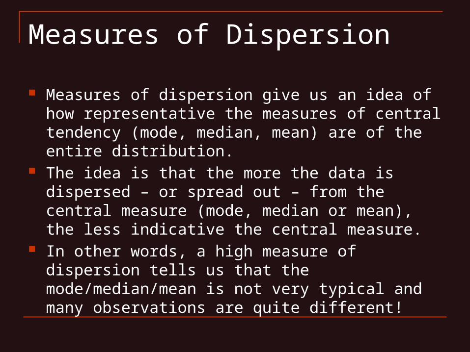
Measures of dispersion give us an idea of how representative the measures of central tendency (mode, median, mean) are of the entire distribution.

The idea is that the more the data is dispersed – or spread out – from the central measure (mode, median or mean), the less indicative the central measure.

In other words, a high measure of dispersion tells us that the mode/median/mean is not very typical and many observations are quite different!

Measures of Dispersion

Measures of dispersion – how dispersed are the observations. Variation ratio Range Interquartile Range Variance & Standard Deviation

Skewness, Kurtosis

Nominal: Variation Ratio

For nominal variables, the variation ratio is the percentage of cases which are not the mode. =1-(number of observations in the mode) / total

number of observations Infrequently used since the variation ratio

really does not tell the reader anything that the mode does not already tell the reader.

Example: Variation Ratio and ModeCanadian Election Study, MBS_B1:Please circle the number that best reflects your opinion.

The government should:1. See to it that everyone has a decent standard of living……1090 (65.7%) = Mode

2. Leave people to get ahead on their own… 384 (23.1%)

8. Not sure ...................185 (11.1%)

Variation Ratio = 34.2%

Note: Unweighted responses are not reflective of the population.

Range

Minimum value to maximum value Useful when you want to know all the possible

responses, for an aggregate policy measures like GDP or other interval/ratio data.

Not very useful for closed-ended survey responses.

In example above, range of real GDP is $338 to $48,589. What does the range tell us about the mean of

$9,089 or the median of $5,194?

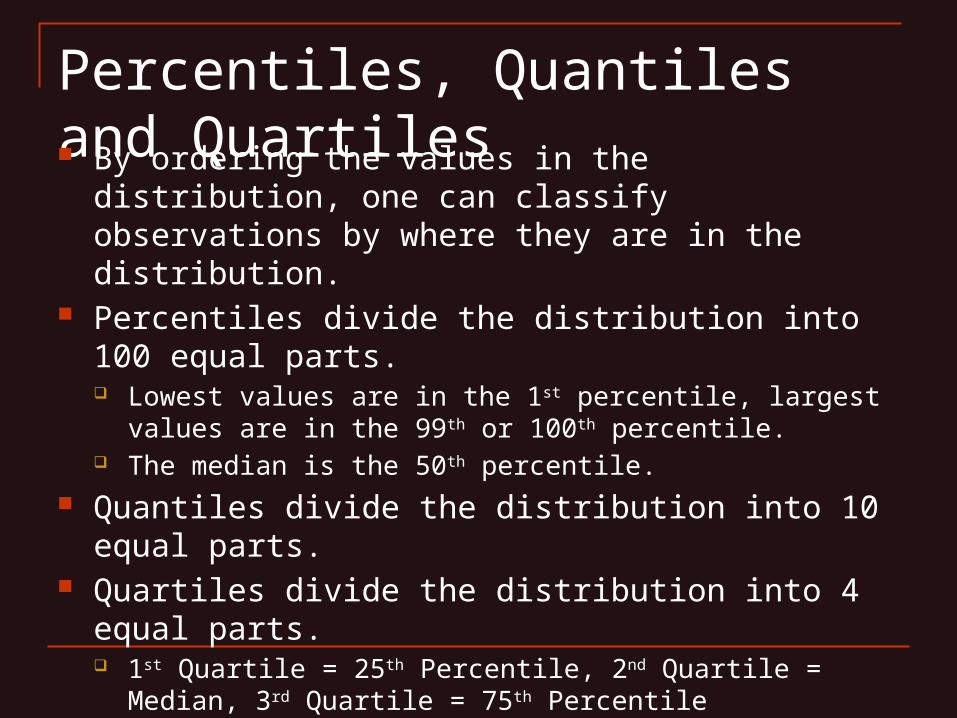
Percentiles, Quantiles and Quartiles By ordering the values in the distribution, one can

classify observations by where they are in the distribution.

Percentiles divide the distribution into 100 equal parts. Lowest values are in the 1st percentile, largest values are in the

99th or 100th percentile. The median is the 50th percentile.

Quantiles divide the distribution into 10 equal parts. Quartiles divide the distribution into 4 equal parts.

1st Quartile = 25th Percentile, 2nd Quartile = Median, 3rd Quartile = 75th Percentile

This matters because quartiles provide us with a measure of dispersion…

Interquartile Range

For closed-ended survey responses, like rating the Conservative Party, finding the interquartile range (or IQR) between the observation value at the 25th percentile and the observation value at the 75th percentile provides more useful information than the full range.

IQR measures the range of the middle half of all observations. A high IQR relative to the range tells the reader that there are

many observations far from the median. A low IQR relative to the range tells the reader that at least half of

all observations are very close to the median.

Calculating the interquartile range Order all of the responses. Identify the observation at the 25th percentile.

Recall: 50th percentile = median. Take the value of this observation.

Identify the observation at the 75th percentile. Take the value of this observation.

Interquartile range= difference between the value of the observation at the 25th percentile and the observation at the 75th percentile.

Ex: Finding 25th and 75th Percentile

Frequency Percent Cum. %

Strongly dislike 0 100 8.64 8.641 76 6.55 15.192 136 11.7 26.893 87 7.51 34.414 85 7.33 41.745 182 15.63 57.376 108 9.26 66.637 146 12.57 79.28 143 12.3 91.59 52 4.5 96

Strongly like 10 46 4 100Total 1,162 100

Source: Canadian Election Study, 2008, CES_MBS_I10a [National Weight]

25th percentile

Median (50th Percentile)= 5

75th percentile

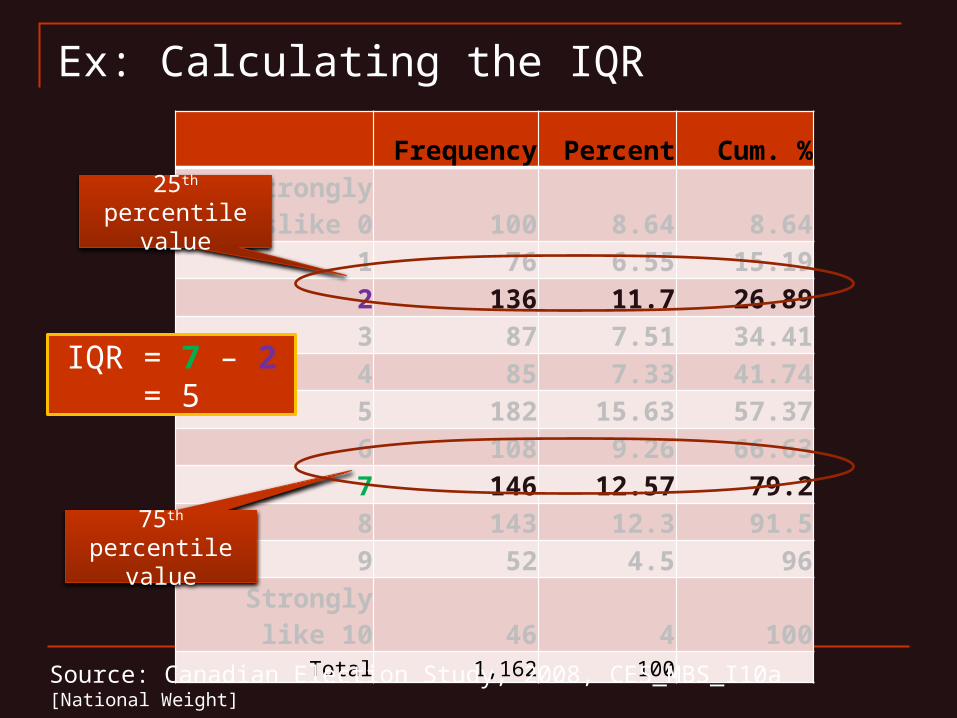
Ex: Calculating the IQR

Frequency Percent Cum. %

Strongly dislike 0 100 8.64 8.641 76 6.55 15.192 136 11.7 26.893 87 7.51 34.414 85 7.33 41.745 182 15.63 57.376 108 9.26 66.637 146 12.57 79.28 143 12.3 91.59 52 4.5 96

Strongly like 10 46 4 100Total 1,162 100

Source: Canadian Election Study, 2008, CES_MBS_I10a [National Weight]

25th percentile value

75th percentile value

IQR = 7 – 2 = 5

Interpreting IQR

The interquartile range for opinions of the Conservative Party (2008) was 5.

An IQR of 5 (with a range of 11) tells us that most observations fall into a relatively narrow range of values. There are few observations with extremely low or

extremely high opinions of the Conservative Party.

Interpreting IQR: Real GDP Example In example above, range of real GDP ran between $338

to $48,589 = $48,251 The median was $5,194. The value of the observation at the 25th percentile is $2,018. The value of the observation at the 75th percentile is $13,532. The interquartile range is $13,532 - $2,018= $11,514.

This tells us that half of all observations are in a relatively narrow range since 11,000 is much smaller than 48,000. Most countries are nowhere near as rich as the richest

countries…

Interpreting IQR: % Pop on $2/day Value of observation at 25th Percentile =

13.1% Value of observation at 75th Percentile =

73.9% What is the interquartile range? Since the range was between 2% and 96.6%,

what does the interquartile range tell us?

Variance Rather than relying on the location of the

value, variance measures dispersion by calculating how far observations are from the mean.

Variance = Average of the distance from the mean of each observation (squared). High variance means that many/most

observations are far from the mean but could be heavily influenced by outliers.

Low variance means that many/most observations are close to the mean.

Formula: Variance

Where N is the total number of observations is the value of each observation is the mean of the set of data The difference between each observation’s value and

the mean is squared before being added to eliminate negative signs.

Result tends to be large relative to the value of the observations.

Standard deviation

Takes square root of variance to put measure in the same unit as the observations. Example: The average rating of the Conservatives is

4.8 and the standard deviation is 2.8. This tells us that the average amount that the ratings

differ from the mean is 2.8 points on the 11 point scale used to measure feeling towards the Conservative Party. In contrast, the variance is 8.0, which can be interpreted as 8

squared points on the 11 point scale. This explanation is confusing and has little intuitive power.

Formula: Standard Deviation

Standard deviation is the square root of variance (S= ),

so the calculations (and symbols)are exactly the same. N is the total number of observations is the value of each observation is the mean of the set of data The difference between each observation’s value and the mean

is squared before being added to eliminate negative signs.

Skewness

If observations are symmetric around the mean there are as many observations less than the mean than there are observations greater than the mean

Skewness measures the extent to which the observations are asymmetric. In other words, skewness tells us whether there are many more

observations above or below the mean. Except skew does not count the observations, skewness

considers the values of the observations. Like mean, skew is sensitive to extreme values.

Skewness Implications

Skewness could have normative implications for policy outcomes and public opinion.

Some bi- and multivariate analyses become more complicated with a skewed distribution.

Interpreting Skewness

Negative skew= most of the observation values are above the mean. Usually this means that most of the observations

(including the median) are below the mean. Positive skew= most of the observation

values are below the mean. Usually this means that most of the observations

(including the median) are below the mean. Skew values close to zero mean that the

distribution is nearly symmetrical.

Conservative Party Skew

Strongly

Dislike

0 1 2 3 4 5 6 7 8 9

Strongly

Like 1

00

2

4

6

8

10

12

14

16

18

%

Source: Canadian Election Study, 2008, CES_MBS_I10a [National Weight]

Mean = 4.8Median = 5

Are more observations above or below the mean?

Conservative Party Skew

Strongly

Dislike

0 1 2 3 4 5 6 7 8 9

Strongly

Like 1

00

2

4

6

8

10

12

14

16

18

%

Source: Canadian Election Study, 2008, CES_MBS_I10a [National Weight]

Mean < Median

More above; therefore skew is negative!

Real GDP Skew

010

2030

Per

cent

0 10000 20000 30000 40000 50000Real GDP per Capita

Source: Gleditsch, K. S. 2002 via Quality of Government (QoG) v6, April 2011

Mean = $9,089.82

Median = $5,194.48

Here, mean > median & skew is positive (1.35).

Kurtosis

Kurtosis measures how tall or flat is the distribution of the variable.

Even with the same variance, some distributions will have more observations in a tall peak near the mean and then be more spread out than a distribution with the observations more concentrated in a shallower, broad peak near the mean. Rarely used in social science.

Kurtosis – Illustrated

Relative to a ‘normal’ mesokurtic distribution (kurtosis=0) Positive kurtosis (“leptokurtic”) means that the observations have

tall peak near the mean. Negative kurtosis values (“platykurtic” – sounds like ‘flat’) means

that the observations are very spread apart with a broad, shallow peak.

Using Descriptive Statistics to Make Comparisons

Compare distributions

A lot A little Not very much

Nothing at all

0

5

10

15

20

25

30

35

40

45

How much have these institutions done to help resolve the conflict in Lebanon (2006)?

U.N.U.S.A.E.U.

Responses are opinions of Canadian adults.

How would you? Describe the opinions portrayed in the

previous slide. What would you say? It may not be very easy.

There is no clear, standard or normal way to make the descriptions.

This is where descriptive statistics proves its use. It is possible to discuss the overall distribution, the

mode, any apparent differences.

How much have these institutions done to help resolve the conflict in Lebanon?Mean Std. Dev Skewness

U. N. 2.5 0.9 -0.04

U. S. A. 2.9 0.9 -0.46

E. U. 2.8 0.8 -0.15

Scale:1 = A lot2 = A little3 = Not very much4 = Nothing at allNote: the median = 3 for all three variables

Comparing Medians

The median for all these variables is three, indicating that: Most Canadians think that the UN, EU and UN

are not doing much or nothing at all There are NOT large differences in opinion

between variables. But there are some differences, and the

table clearly indicates what those differences are in a concise manner.

Comparing Means

Mean Std. Dev Skewness

U. N. 2.5 0.9 -0.04

U. S. A. 2.9 0.9 -0.46

E. U. 2.8 0.8 -0.15

Scale:1 = A lot2 = A little3 = Not very much4 = Nothing at all

The mean for the U.N. is lower than the mean response for USA and EU, telling us that Canadians thought that the U.N. was doing [slightly] more to resolve the conflict than the EU and the USA.

The low UN mean is sensitive to the relatively high number of respondents who said the UN was doing “a lot.”

Comparing dispersion

Mean Std. Dev Skewness

U. N. 2.5 0.9 -0.04

U. S. A. 2.9 0.9 -0.46

E. U. 2.8 0.8 -0.15

Scale:1 = A lot2 = A little3 = Not very much4 = Nothing at all

The standard deviation is about the same, indicating that the dispersion of opinion is about the same.

How much have these institutions done to help resolve the conflict in Lebanon?Mean Std. Dev Skewness

U. N. 2.5 0.9 -0.04

U. S. A. 2.9 0.9 -0.46

E. U. 2.8 0.8 -0.15

Scale:1 = A lot2 = A little3 = Not very much4 = Nothing at all

All three variables skew negative, indicating that more opinions are “above” the mean. With the scale used for this variable, this means that more than half of all respondents thought that the UN, US and EU were doing “not very much” or “nothing at all.” In particular, the U.S.A., was seen by many as not doing very much. Can you see this in the chart?

Comparing attitudes towards the federal parties

Mean Median Std. Dev IQR Skew

Conservative 4.8 5 2.8 5 -0.1

Liberal 4.7 5 2.3 3 -0.16

NDP 4.3 5 2.5 4 0.10

Greens 3.8 4 2.4 3 0.19

Bloc Quebecois

2.5 2 2.8 5 0.94

Which party, on average, was the most popular in 2008? Least popular? Is one party much more or much less popular

than the others?

Source: Canadian Election Study, 2008, CES_MBS_I10a-e [National Weight]

Comparing attitudes towards the federal parties

Mean Median Std. Dev IQR Skew

Conservative 4.8 5 2.8 5 -0.1

Liberal 4.7 5 2.3 3 -0.16

NDP 4.3 5 2.5 4 0.10

Towards which of the three largest parties is the widest range of feelings? Narrowest? From this table, could you conclude that most

Canadians feel much the same way about one party?

Do Canadians seem badly divided about any party?

Source: Canadian Election Study, 2008, CES_MBS_I10a-e [National Weight]