Embed Size (px)
Citation preview
Description, Modeling and Simulation Results
of a Test System for Voltage Stability Analysis
Version 6. November 2013
Thierry VAN CUTSEM Lampros PAPANGELIS
University of Liege, Belgium
Contents
1 System overview 4
2 Models and data 7
2.1 Network data . . . . . . . . . . . . . . . . . . . . . . . . . . . . . . . . . . . . . . . . . . 7
2.2 Operating point data . . . . . . . . . . . . . . . . . . . . . . . . . . . . . . . . . . . . . . 12
2.2.1 Operating point A . . . . . . . . . . . . . . . . . . . . . . . . . . . . . . . . . . . 12
2.2.2 Operating point B . . . . . . . . . . . . . . . . . . . . . . . . . . . . . . . . . . . . 14
2.3 Synchronous machine data . . . . . . . . . . . . . . . . . . . . . . . . . . . . . . . . . . . 16
2.4 Exciter, automatic voltage regulator and power system stabilizer model and data . . . . . . . 18
2.5 Overexcitation limiter model and data . . . . . . . . . . . . . . . . . . . . . . . . . . . . . 19
2.6 Generator capability curves . . . . . . . . . . . . . . . . . . . . . . . . . . . . . . . . . . . 21
2.7 Turbine model and data . . . . . . . . . . . . . . . . . . . . . . . . . . . . . . . . . . . . . 26
2.8 Speed governor model and data . . . . . . . . . . . . . . . . . . . . . . . . . . . . . . . . . 26
2.9 Load data . . . . . . . . . . . . . . . . . . . . . . . . . . . . . . . . . . . . . . . . . . . . 27
2.10 Load tap changer data . . . . . . . . . . . . . . . . . . . . . . . . . . . . . . . . . . . . . . 27
3 Dynamic responses to contingencies 27
3.1 Operating point A . . . . . . . . . . . . . . . . . . . . . . . . . . . . . . . . . . . . . . . . 27
3.1.1 Disturbance . . . . . . . . . . . . . . . . . . . . . . . . . . . . . . . . . . . . . . . 27
3.1.2 Voltages . . . . . . . . . . . . . . . . . . . . . . . . . . . . . . . . . . . . . . . . . 28
3.1.3 Generator field currents and terminal voltages . . . . . . . . . . . . . . . . . . . . . 28
3.1.4 Transformer ratios . . . . . . . . . . . . . . . . . . . . . . . . . . . . . . . . . . . 31
3.1.5 Rotor speeds and angles . . . . . . . . . . . . . . . . . . . . . . . . . . . . . . . . 32
2
3.2 Operating point B . . . . . . . . . . . . . . . . . . . . . . . . . . . . . . . . . . . . . . . . 34
4 Examples of preventive security margin computations 38
4.1 Secure operation limit: definition . . . . . . . . . . . . . . . . . . . . . . . . . . . . . . . . 38
4.2 Pre-contingency stress . . . . . . . . . . . . . . . . . . . . . . . . . . . . . . . . . . . . . 38
4.3 SOL with respect to the contingency of Section 3.1.1 . . . . . . . . . . . . . . . . . . . . . 40
4.4 SOL with respect to generator outages . . . . . . . . . . . . . . . . . . . . . . . . . . . . . 41
4.5 SOL with respect to line outages . . . . . . . . . . . . . . . . . . . . . . . . . . . . . . . . 42
5 Examples of corrective post-disturbance control 43
5.1 Modified tap changer control . . . . . . . . . . . . . . . . . . . . . . . . . . . . . . . . . . 43
5.2 Undervoltage load shedding . . . . . . . . . . . . . . . . . . . . . . . . . . . . . . . . . . 45
6 Long-term voltage instability analysis through sensitivities 47
3

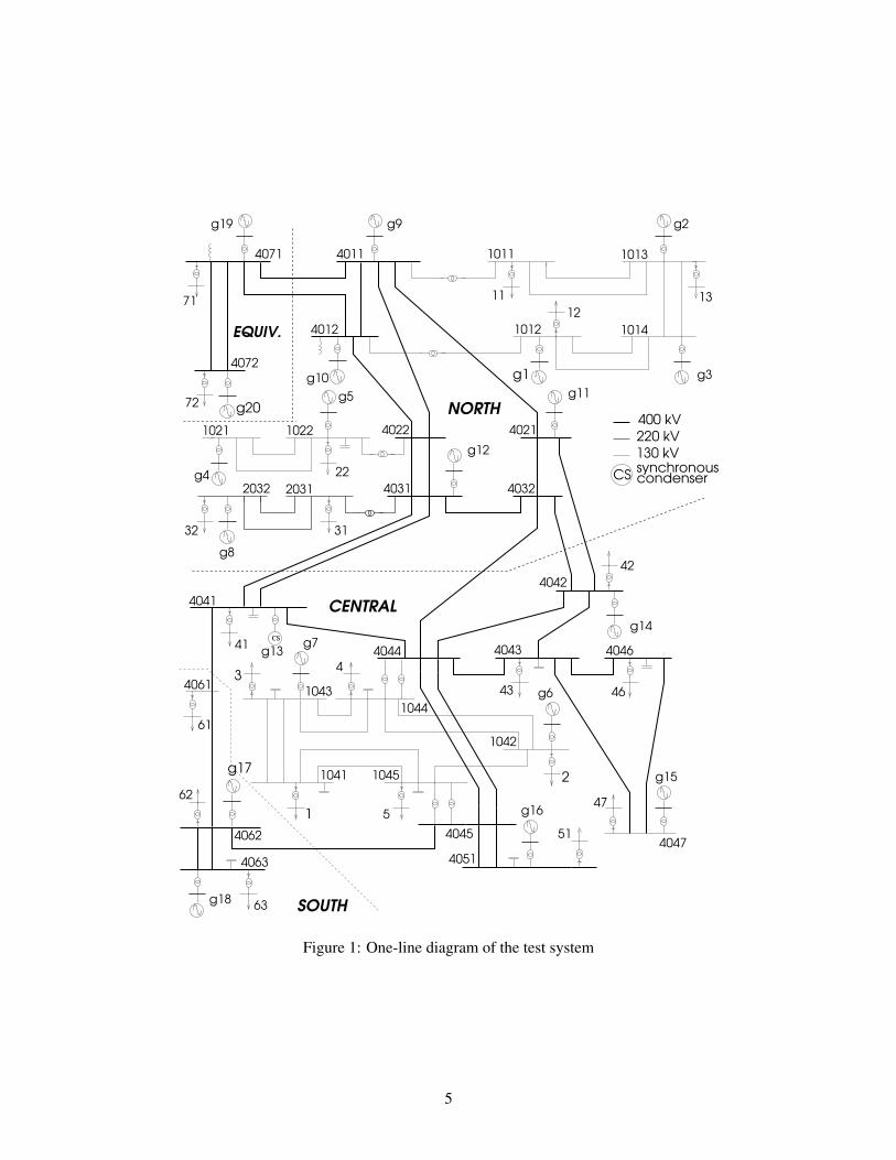
1 System overview
The proposed system is a variant of the so-called Nordic32 test system, proposed by K. Walve1 and detailedin [1]. As indicated in this reference, the system is fictitious but similar to the Swedish and Nordic system(at the time of setting up this test system).
The one-line diagram is shown in Fig. 1.
This system consists of four areas:
• “North” with hydro generation and some load
• “Central” with much load and thermal power generation
• “Equiv” connected to the “North”, it includes a very simple equivalent of an external system
• “South” with thermal generation, rather loosely connected to the rest of the system.
The system has rather long transmission lines of 400-kV nominal voltage. Figure 2 shows the structureof the 400-kV backbone, rendering the geographic locations of the stations. Five lines are equipped withseries compensation; the percentage of compensation is shown in the figure. The model also includes arepresentation of some regional systems operating at 220 and 130 kV, respectively (see Fig. 1).
Table 1 gives the active power load and generation in each area and for the whole system.
Table 1: Active power load and generationarea generated power (MW) consumed power (MW)
North 4628.5 1180.0Central 2850.0 6190.0South 1590.0 1390.0Equiv 2437.4 2300.0total 11505.9 11060.0
The nominal frequency is 50 Hz. Frequency is controlled through the speed governors of the hydro gen-erators in the “North” and “Equiv” areas only (see Fig. 1). g20 is an equivalent generator, with a largeparticipation in primary frequency control. The thermal units of the Central and South areas do not partici-pate in this control.
The system is heavily loaded with large transfers essentially from North to Central areas. Secure systemoperation is limited by transient (angle) and long-term voltage instability. The contingencies likely to yieldvoltage instability are:
• the tripping of a line in the North-Central corridor, forcing the North-Central power to flow over theremaining lines;
1at that time with Svenska Kraftn’et, Sweden
4
g15
g11
g20
g19
g16
g17
g18
g2
g6
g7
g14
g13
g8
g12
g4
g5
g10 g3g1
g9
4011
4012
1011
1012 1014
1013
10221021
2031
cs
404640434044
40324031
4022 4021
4071
4072
4041
1042
10451041
4063
40611043
1044
4047
4051
40454062
400 kV
220 kV
130 kV synchronous condenserCS
NORTH
CENTRAL
EQUIV.
SOUTH
4042
2032
41
1 5
3
2
51
47
42
61
62
63
4
43 46
3132
22
11 13
12
72
71
Figure 1: One-line diagram of the test system
5
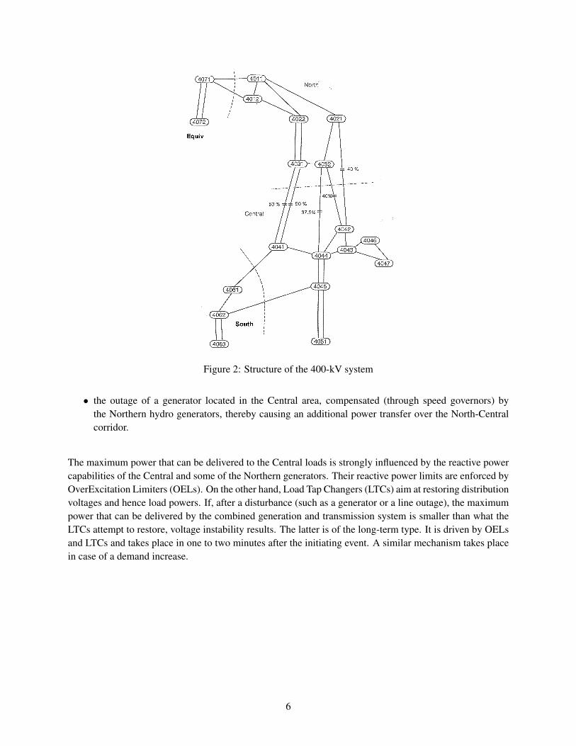
Figure 2: Structure of the 400-kV system
• the outage of a generator located in the Central area, compensated (through speed governors) bythe Northern hydro generators, thereby causing an additional power transfer over the North-Centralcorridor.
The maximum power that can be delivered to the Central loads is strongly influenced by the reactive powercapabilities of the Central and some of the Northern generators. Their reactive power limits are enforced byOverExcitation Limiters (OELs). On the other hand, Load Tap Changers (LTCs) aim at restoring distributionvoltages and hence load powers. If, after a disturbance (such as a generator or a line outage), the maximumpower that can be delivered by the combined generation and transmission system is smaller than what theLTCs attempt to restore, voltage instability results. The latter is of the long-term type. It is driven by OELsand LTCs and takes place in one to two minutes after the initiating event. A similar mechanism takes placein case of a demand increase.
6
2 Models and data
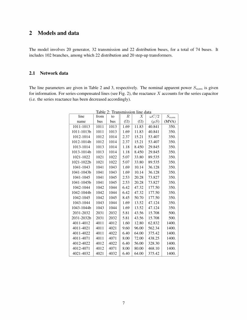
The model involves 20 generator, 32 transmission and 22 distribution buses, for a total of 74 buses. Itincludes 102 branches, among which 22 distribution and 20 step-up transformers.
2.1 Network data
The line parameters are given in Table 2 and 3, respectively. The nominal apparent power Snom is givenfor information. For series-compensated lines (see Fig. 2), the reactance X accounts for the series capacitor(i.e. the series reactance has been decreased accordingly).
Table 2: Transmission line dataline from to R X ωC/2 Snom
name bus bus (Ω) (Ω) (µS) (MVA)1011-1013 1011 1013 1.69 11.83 40.841 350.1011-1013b 1011 1013 1.69 11.83 40.841 350.1012-1014 1012 1014 2.37 15.21 53.407 350.1012-1014b 1012 1014 2.37 15.21 53.407 350.1013-1014 1013 1014 1.18 8.450 29.845 350.1013-1014b 1013 1014 1.18 8.450 29.845 350.1021-1022 1021 1022 5.07 33.80 89.535 350.1021-1022b 1021 1022 5.07 33.80 89.535 350.1041-1043 1041 1043 1.69 10.14 36.128 350.1041-1043b 1041 1043 1.69 10.14 36.128 350.1041-1045 1041 1045 2.53 20.28 73.827 350.1041-1045b 1041 1045 2.53 20.28 73.827 350.1042-1044 1042 1044 6.42 47.32 177.50 350.1042-1044b 1042 1044 6.42 47.32 177.50 350.1042-1045 1042 1045 8.45 50.70 177.50 350.1043-1044 1043 1044 1.69 13.52 47.124 350.1043-1044b 1043 1044 1.69 13.52 47.124 350.2031-2032 2031 2032 5.81 43.56 15.708 500.2031-2032b 2031 2032 5.81 43.56 15.708 500.4011-4012 4011 4012 1.60 12.80 62.832 1400.4011-4021 4011 4021 9.60 96.00 562.34 1400.4011-4022 4011 4022 6.40 64.00 375.42 1400.4011-4071 4011 4071 8.00 72.00 438.25 1400.4012-4022 4012 4022 6.40 56.00 328.30 1400.4012-4071 4012 4071 8.00 80.00 468.10 1400.4021-4032 4021 4032 6.40 64.00 375.42 1400.
7
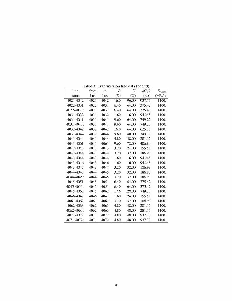
Table 3: Transmission line data (cont’d)line from to R X ωC/2 Snom
name bus bus (Ω) (Ω) (µS) (MVA)4021-4042 4021 4042 16.0 96.00 937.77 1400.4022-4031 4022 4031 6.40 64.00 375.42 1400.4022-4031b 4022 4031 6.40 64.00 375.42 1400.4031-4032 4031 4032 1.60 16.00 94.248 1400.4031-4041 4031 4041 9.60 64.00 749.27 1400.4031-4041b 4031 4041 9.60 64.00 749.27 1400.4032-4042 4032 4042 16.0 64.00 625.18 1400.4032-4044 4032 4044 9.60 80.00 749.27 1400.4041-4044 4041 4044 4.80 48.00 281.17 1400.4041-4061 4041 4061 9.60 72.00 406.84 1400.4042-4043 4042 4043 3.20 24.00 155.51 1400.4042-4044 4042 4044 3.20 32.00 186.93 1400.4043-4044 4043 4044 1.60 16.00 94.248 1400.4043-4046 4043 4046 1.60 16.00 94.248 1400.4043-4047 4043 4047 3.20 32.00 186.93 1400.4044-4045 4044 4045 3.20 32.00 186.93 1400.4044-4045b 4044 4045 3.20 32.00 186.93 1400.4045-4051 4045 4051 6.40 64.00 375.42 1400.4045-4051b 4045 4051 6.40 64.00 375.42 1400.4045-4062 4045 4062 17.6 128.00 749.27 1400.4046-4047 4046 4047 1.60 24.00 155.51 1400.4061-4062 4061 4062 3.20 32.00 186.93 1400.4062-4063 4062 4063 4.80 48.00 281.17 1400.4062-4063b 4062 4063 4.80 48.00 281.17 1400.4071-4072 4071 4072 4.80 48.00 937.77 1400.4071-4072b 4071 4072 4.80 48.00 937.77 1400.
8
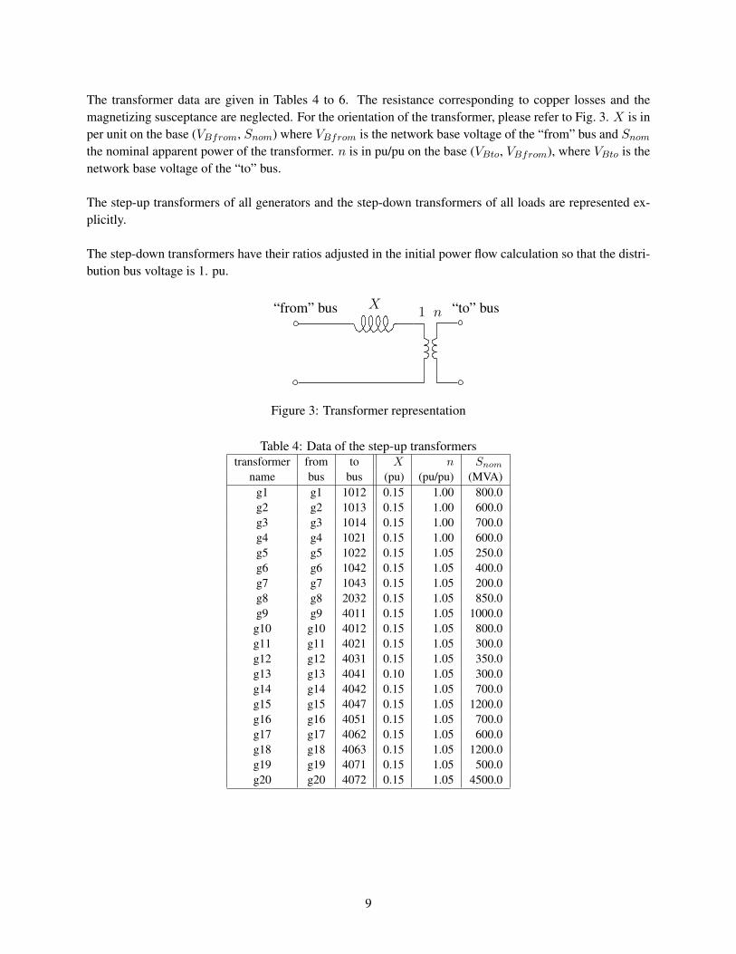
The transformer data are given in Tables 4 to 6. The resistance corresponding to copper losses and themagnetizing susceptance are neglected. For the orientation of the transformer, please refer to Fig. 3. X is inper unit on the base (VBfrom, Snom) where VBfrom is the network base voltage of the “from” bus and Snom
the nominal apparent power of the transformer. n is in pu/pu on the base (VBto, VBfrom), where VBto is thenetwork base voltage of the “to” bus.
The step-up transformers of all generators and the step-down transformers of all loads are represented ex-plicitly.
The step-down transformers have their ratios adjusted in the initial power flow calculation so that the distri-bution bus voltage is 1. pu.
“to” bus1 nX“from” bus
Figure 3: Transformer representation
Table 4: Data of the step-up transformerstransformer from to X n Snom
name bus bus (pu) (pu/pu) (MVA)g1 g1 1012 0.15 1.00 800.0g2 g2 1013 0.15 1.00 600.0g3 g3 1014 0.15 1.00 700.0g4 g4 1021 0.15 1.00 600.0g5 g5 1022 0.15 1.05 250.0g6 g6 1042 0.15 1.05 400.0g7 g7 1043 0.15 1.05 200.0g8 g8 2032 0.15 1.05 850.0g9 g9 4011 0.15 1.05 1000.0g10 g10 4012 0.15 1.05 800.0g11 g11 4021 0.15 1.05 300.0g12 g12 4031 0.15 1.05 350.0g13 g13 4041 0.10 1.05 300.0g14 g14 4042 0.15 1.05 700.0g15 g15 4047 0.15 1.05 1200.0g16 g16 4051 0.15 1.05 700.0g17 g17 4062 0.15 1.05 600.0g18 g18 4063 0.15 1.05 1200.0g19 g19 4071 0.15 1.05 500.0g20 g20 4072 0.15 1.05 4500.0
9
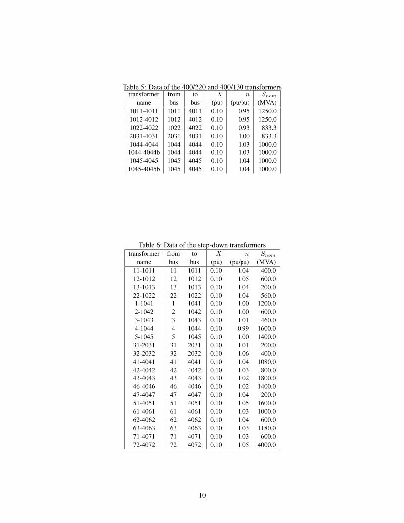
Table 5: Data of the 400/220 and 400/130 transformerstransformer from to X n Snom
name bus bus (pu) (pu/pu) (MVA)1011-4011 1011 4011 0.10 0.95 1250.01012-4012 1012 4012 0.10 0.95 1250.01022-4022 1022 4022 0.10 0.93 833.32031-4031 2031 4031 0.10 1.00 833.31044-4044 1044 4044 0.10 1.03 1000.01044-4044b 1044 4044 0.10 1.03 1000.01045-4045 1045 4045 0.10 1.04 1000.01045-4045b 1045 4045 0.10 1.04 1000.0
Table 6: Data of the step-down transformerstransformer from to X n Snom
name bus bus (pu) (pu/pu) (MVA)11-1011 11 1011 0.10 1.04 400.012-1012 12 1012 0.10 1.05 600.013-1013 13 1013 0.10 1.04 200.022-1022 22 1022 0.10 1.04 560.01-1041 1 1041 0.10 1.00 1200.02-1042 2 1042 0.10 1.00 600.03-1043 3 1043 0.10 1.01 460.04-1044 4 1044 0.10 0.99 1600.05-1045 5 1045 0.10 1.00 1400.031-2031 31 2031 0.10 1.01 200.032-2032 32 2032 0.10 1.06 400.041-4041 41 4041 0.10 1.04 1080.042-4042 42 4042 0.10 1.03 800.043-4043 43 4043 0.10 1.02 1800.046-4046 46 4046 0.10 1.02 1400.047-4047 47 4047 0.10 1.04 200.051-4051 51 4051 0.10 1.05 1600.061-4061 61 4061 0.10 1.03 1000.062-4062 62 4062 0.10 1.04 600.063-4063 63 4063 0.10 1.03 1180.071-4071 71 4071 0.10 1.03 600.072-4072 72 4072 0.10 1.05 4000.0
10
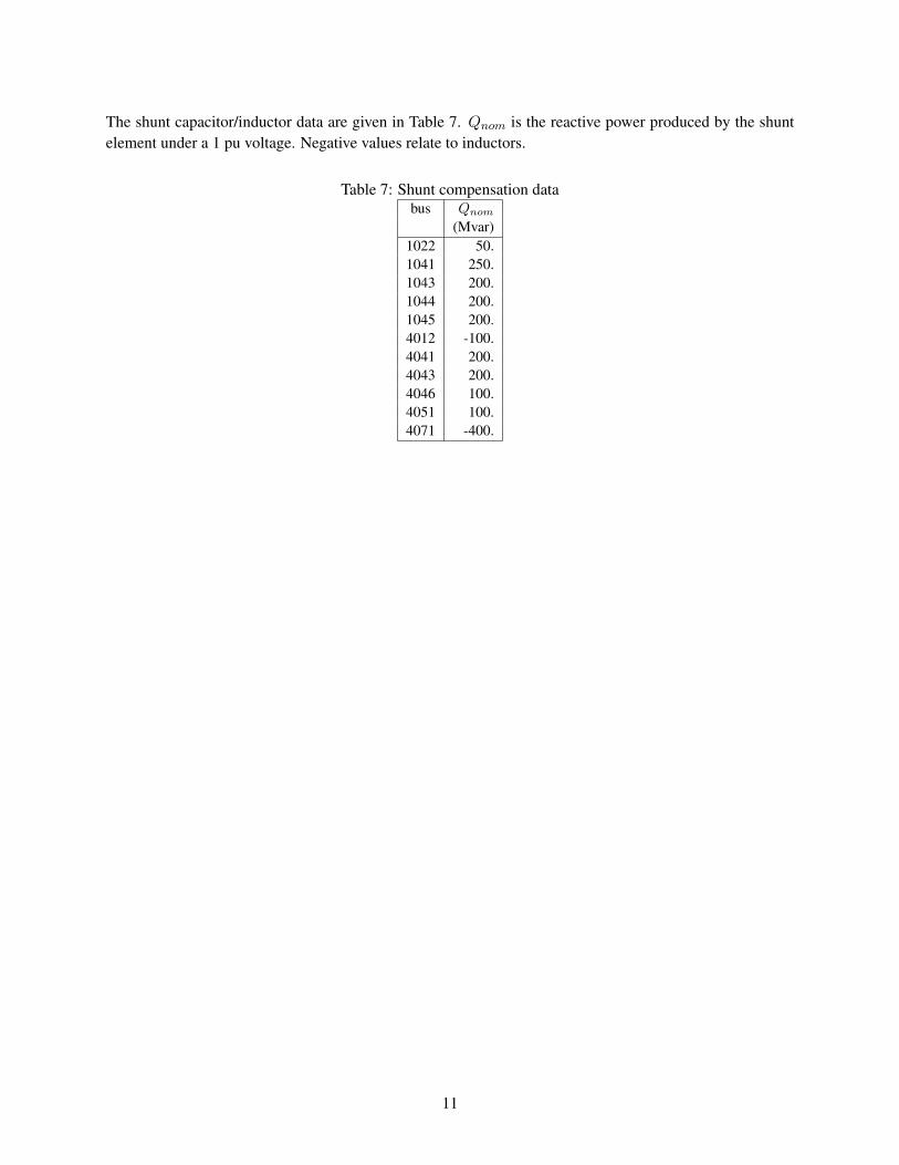
The shunt capacitor/inductor data are given in Table 7. Qnom is the reactive power produced by the shuntelement under a 1 pu voltage. Negative values relate to inductors.
Table 7: Shunt compensation databus Qnom
(Mvar)1022 50.1041 250.1043 200.1044 200.1045 200.4012 -100.4041 200.4043 200.4046 100.4051 100.4071 -400.
11
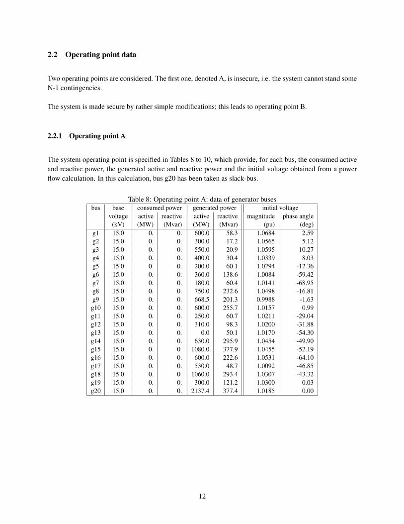
2.2 Operating point data
Two operating points are considered. The first one, denoted A, is insecure, i.e. the system cannot stand someN-1 contingencies.
The system is made secure by rather simple modifications; this leads to operating point B.
2.2.1 Operating point A
The system operating point is specified in Tables 8 to 10, which provide, for each bus, the consumed activeand reactive power, the generated active and reactive power and the initial voltage obtained from a powerflow calculation. In this calculation, bus g20 has been taken as slack-bus.
Table 8: Operating point A: data of generator busesbus base consumed power generated power initial voltage
voltage active reactive active reactive magnitude phase angle(kV) (MW) (Mvar) (MW) (Mvar) (pu) (deg)
g1 15.0 0. 0. 600.0 58.3 1.0684 2.59g2 15.0 0. 0. 300.0 17.2 1.0565 5.12g3 15.0 0. 0. 550.0 20.9 1.0595 10.27g4 15.0 0. 0. 400.0 30.4 1.0339 8.03g5 15.0 0. 0. 200.0 60.1 1.0294 -12.36g6 15.0 0. 0. 360.0 138.6 1.0084 -59.42g7 15.0 0. 0. 180.0 60.4 1.0141 -68.95g8 15.0 0. 0. 750.0 232.6 1.0498 -16.81g9 15.0 0. 0. 668.5 201.3 0.9988 -1.63g10 15.0 0. 0. 600.0 255.7 1.0157 0.99g11 15.0 0. 0. 250.0 60.7 1.0211 -29.04g12 15.0 0. 0. 310.0 98.3 1.0200 -31.88g13 15.0 0. 0. 0.0 50.1 1.0170 -54.30g14 15.0 0. 0. 630.0 295.9 1.0454 -49.90g15 15.0 0. 0. 1080.0 377.9 1.0455 -52.19g16 15.0 0. 0. 600.0 222.6 1.0531 -64.10g17 15.0 0. 0. 530.0 48.7 1.0092 -46.85g18 15.0 0. 0. 1060.0 293.4 1.0307 -43.32g19 15.0 0. 0. 300.0 121.2 1.0300 0.03g20 15.0 0. 0. 2137.4 377.4 1.0185 0.00
12
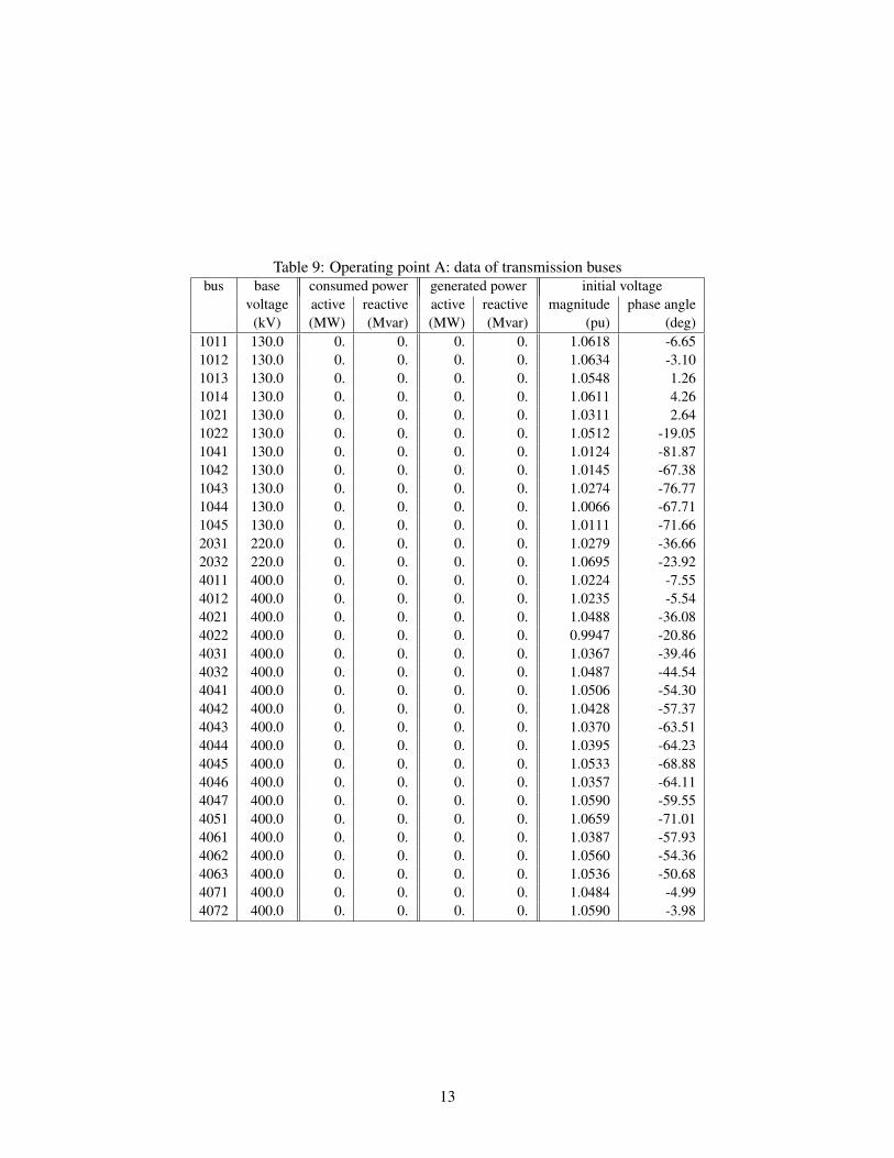
Table 9: Operating point A: data of transmission busesbus base consumed power generated power initial voltage
voltage active reactive active reactive magnitude phase angle(kV) (MW) (Mvar) (MW) (Mvar) (pu) (deg)
1011 130.0 0. 0. 0. 0. 1.0618 -6.651012 130.0 0. 0. 0. 0. 1.0634 -3.101013 130.0 0. 0. 0. 0. 1.0548 1.261014 130.0 0. 0. 0. 0. 1.0611 4.261021 130.0 0. 0. 0. 0. 1.0311 2.641022 130.0 0. 0. 0. 0. 1.0512 -19.051041 130.0 0. 0. 0. 0. 1.0124 -81.871042 130.0 0. 0. 0. 0. 1.0145 -67.381043 130.0 0. 0. 0. 0. 1.0274 -76.771044 130.0 0. 0. 0. 0. 1.0066 -67.711045 130.0 0. 0. 0. 0. 1.0111 -71.662031 220.0 0. 0. 0. 0. 1.0279 -36.662032 220.0 0. 0. 0. 0. 1.0695 -23.924011 400.0 0. 0. 0. 0. 1.0224 -7.554012 400.0 0. 0. 0. 0. 1.0235 -5.544021 400.0 0. 0. 0. 0. 1.0488 -36.084022 400.0 0. 0. 0. 0. 0.9947 -20.864031 400.0 0. 0. 0. 0. 1.0367 -39.464032 400.0 0. 0. 0. 0. 1.0487 -44.544041 400.0 0. 0. 0. 0. 1.0506 -54.304042 400.0 0. 0. 0. 0. 1.0428 -57.374043 400.0 0. 0. 0. 0. 1.0370 -63.514044 400.0 0. 0. 0. 0. 1.0395 -64.234045 400.0 0. 0. 0. 0. 1.0533 -68.884046 400.0 0. 0. 0. 0. 1.0357 -64.114047 400.0 0. 0. 0. 0. 1.0590 -59.554051 400.0 0. 0. 0. 0. 1.0659 -71.014061 400.0 0. 0. 0. 0. 1.0387 -57.934062 400.0 0. 0. 0. 0. 1.0560 -54.364063 400.0 0. 0. 0. 0. 1.0536 -50.684071 400.0 0. 0. 0. 0. 1.0484 -4.994072 400.0 0. 0. 0. 0. 1.0590 -3.98
13
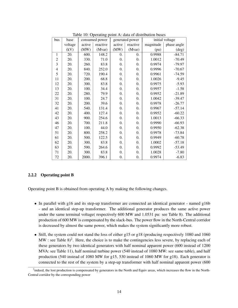
Table 10: Operating point A: data of distribution busesbus base consumed power generated power initial voltage
voltage active reactive active reactive magnitude phase angle(kV) (MW) (Mvar) (MW) (Mvar) (pu) (deg)
1 20. 600. 148.2 0. 0. 0.9988 -84.712 20. 330. 71.0 0. 0. 1.0012 -70.493 20. 260. 83.8 0. 0. 0.9974 -79.974 20. 840. 252.0 0. 0. 0.9996 -70.675 20. 720. 190.4 0. 0. 0.9961 -74.5911 20. 200. 68.8 0. 0. 1.0026 -9.4512 20. 300. 83.8 0. 0. 0.9975 -5.9313 20. 100. 34.4 0. 0. 0.9957 -1.5822 20. 280. 79.9 0. 0. 0.9952 -21.8931 20. 100. 24.7 0. 0. 1.0042 -39.4732 20. 200. 39.6 0. 0. 0.9978 -26.7741 20. 540. 131.4 0. 0. 0.9967 -57.1442 20. 400. 127.4 0. 0. 0.9952 -60.2243 20. 900. 254.6 0. 0. 1.0013 -66.3346 20. 700. 211.8 0. 0. 0.9990 -66.9347 20. 100. 44.0 0. 0. 0.9950 -62.3851 20. 800. 258.2 0. 0. 0.9978 -73.8461 20. 500. 122.5 0. 0. 0.9949 -60.7862 20. 300. 83.8 0. 0. 1.0002 -57.1863 20. 590. 264.6 0. 0. 0.9992 -53.4971 20. 300. 83.8 0. 0. 1.0028 -7.8072 20. 2000. 396.1 0. 0. 0.9974 -6.83
2.2.2 Operating point B
Operating point B is obtained from operating A by making the following changes.
• In parallel with g16 and its step-up transformer are connected an identical generator - named g16b- and an identical step-up transformer. The additional generator produces the same active powerunder the same terminal voltage( respectively 600 MW and 1.0531 pu: see Table 8). The additionalproduction of 600 MW is compensated by the slack-bus. The power flow in the North-Central corridoris decreased by almost the same power, which makes the system significantly more robust.
• Still, the system could not stand the loss of either g15 or g18 (producing respectively 1080 and 1060MW : see Table 8)2. Here, the choice is to make the contingencies less severe, by replacing each ofthese generators by two identical generators with half nominal apparent power (600 instead of 1200MVA: see Table 11), half nominal turbine power (540 instead of 1080 MW: see same table), and halfproduction (540 instead of 1080 MW for g15, 530 instead of 1060 MW for g18). Each generator isconnected to the rest of the system by a step-up transformer with half nominal apparent power (600
2indeed, the lost production is compensated by generators in the North and Equiv areas, which increases the flow in the North-Central corridor by the corresponding power
14
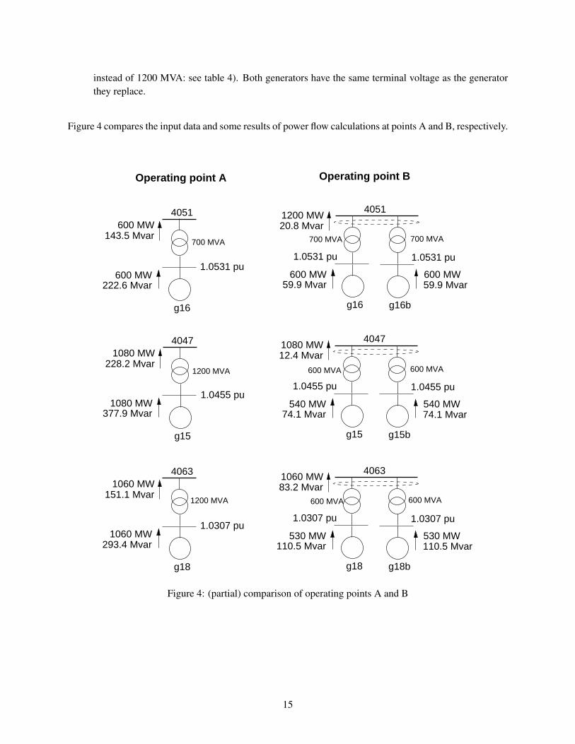
instead of 1200 MVA: see table 4). Both generators have the same terminal voltage as the generatorthey replace.
Figure 4 compares the input data and some results of power flow calculations at points A and B, respectively.
Operating point A Operating point B
4051
g16
1.0531 pu600 MW
222.6 Mvar
600 MW143.5 Mvar
4047
g15
1.0455 pu1080 MW
1080 MW228.2 Mvar
4063
g18
1.0307 pu1060 MW
1060 MW151.1 Mvar
377.9 Mvar
293.4 Mvar
4051
g16
1.0531 pu
600 MW59.9 Mvar
1200 MW20.8 Mvar
g16b
600 MW59.9 Mvar
1.0531 pu
4047
g15
1.0455 pu
540 MW74.1 Mvar
1080 MW12.4 Mvar
g15b
540 MW74.1 Mvar
1.0455 pu
4063
g18
1.0307 pu
530 MW110.5 Mvar
1060 MW83.2 Mvar
g18b
530 MW110.5 Mvar
1.0307 pu
700 MVA 700 MVA 700 MVA
1200 MVA 600 MVA600 MVA
600 MVA600 MVA1200 MVA
Figure 4: (partial) comparison of operating points A and B
15
2.3 Synchronous machine data
Synchronous machines are represented by a standard model (e.g. [2]) with three rotor winding for thesalient-pole machines of hydro power plants, and four rotor windings for the round-rotor machines of ther-mal plants. g13 is a synchronous condenser.
The nominal apparent power Snom of each generator together with the nominal active power Pnom of itsturbine are given in Table 11. As can be seen, the generator power factor, computed as Pnom/Snom, is 0.95for the hydro plants (North and Equiv areas) and 0.90 for the thermal plants (Central and South areas, wheremost of the load is located).
Table 11: Nominal apparent powers of synchronous machines and nominal active powers of their turbinesgener. Snom Pnom
(MVA) (MW)g1 800. 760.0g2 600. 570.0g3 700. 665.0g4 600. 570.0g5 250. 237.5g6 400. 360.0g7 200. 180.0g8 850. 807.5g9 1000. 950.0g10 800. 760.0g11 300. 285.0g12 350. 332.5g13 300. -g14 700. 630.0g15 1200. 1080.0g16 700. 630.0g17 600. 540.0g18 1200. 1080.0g19 500. 475.0g20 4500. 4275.0
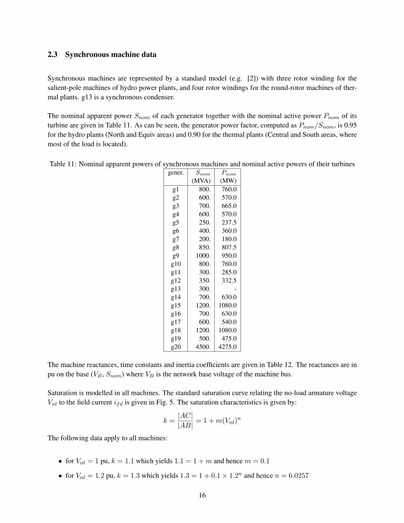
The machine reactances, time constants and inertia coefficients are given in Table 12. The reactances are inpu on the base (VB , Snom) where VB is the network base voltage of the machine bus.
Saturation is modelled in all machines. The standard saturation curve relating the no-load armature voltageVnl to the field current ifd is given in Fig. 5. The saturation characteristics is given by:
k =|AC||AB|
= 1 +m(Vnl)n
The following data apply to all machines:
• for Vnl = 1 pu, k = 1.1 which yields 1.1 = 1 +m and hence m = 0.1
• for Vnl = 1.2 pu, k = 1.3 which yields 1.3 = 1 + 0.1× 1.2n and hence n = 6.0257
16
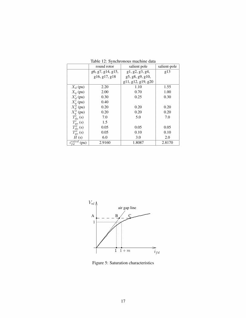
Table 12: Synchronous machine dataround rotor salient pole salient-pole
g6, g7, g14, g15, g1, g2, g3, g4, g13g16, g17, g18 g5, g8, g9, g10,
g11, g12, g19, g20Xd (pu) 2.20 1.10 1.55Xq (pu) 2.00 0.70 1.00X ′
d (pu) 0.30 0.25 0.30X ′
q (pu) 0.40X ′′
d (pu) 0.20 0.20 0.20X ′′
q (pu) 0.20 0.20 0.20T ′do (s) 7.0 5.0 7.0
T ′qo (s) 1.5
T ′′do (s) 0.05 0.05 0.05
T ′′qo (s) 0.05 0.10 0.10H (s) 6.0 3.0 2.0
iratedfd (pu) 2.9160 1.8087 2.8170
air gap line
1 1 +m1
A B C
Vnl
ifd
1
Figure 5: Saturation characteristics
17
• (unsaturated) leakage reactance Xℓ = 0.15 pu in both axes.
The last row in Table 12 provides the generator field currents iratedfd under rated operating conditions, i.e.when the machine operates with:
V = 1
P = Pnom
S = Snom ⇔√
P 2nom +Q2 = Snom ⇔ Q =
√S2nom − P 2
nom
where P , V and S are in per unit. The iratedfd values are in per unit on a base such that ifd = 1 pu when thegenerator operates at no load with a 1 pu terminal voltage and without saturation (operation on the air gapline). This corresponds to the leftmost point on the abscissa in Fig. 5.
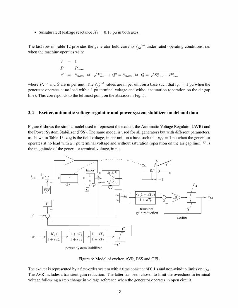
2.4 Exciter, automatic voltage regulator and power system stabilizer model and data
Figure 6 shows the simple model used to represent the exciter, the Automatic Voltage Regulator (AVR) andthe Power System Stabilizer (PSS). The same model is used for all generators but with different parameters,as shown in Table 13. vfd is the field voltage, in per unit on a base such that vfd = 1 pu when the generatoroperates at no load with a 1 pu terminal voltage and without saturation (operation on the air gap line). V isthe magnitude of the generator terminal voltage, in pu.
C
2 3
+
−vfd
G(1 + sTa)
1 + sTbV o
−
+
V
min
−
+
ilimfd
ifd
1
s
1 + sT1
1 + sT2
1 + sT1
1 + sT2
ωKps
1 + sTw
L1
exciter
transientgain reduction
power system stabilizer
f
−1
r
0−0.1
−1
10
0
L21
y
y < 0
1
s
timer
+
y ≥ 0
−C
Figure 6: Model of exciter, AVR, PSS and OEL
The exciter is represented by a first-order system with a time constant of 0.1 s and non-windup limits on vfd.The AVR includes a transient gain reduction. The latter has been chosen to limit the overshoot in terminalvoltage following a step change in voltage reference when the generator operates in open circuit.
18
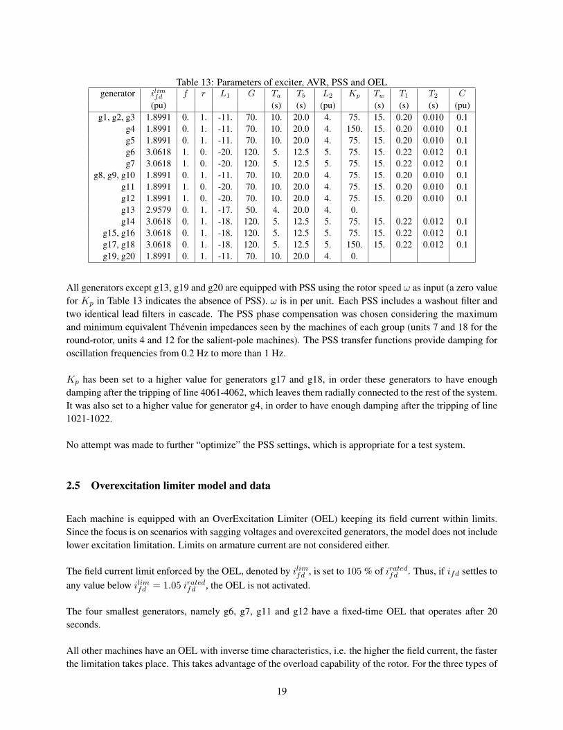
Table 13: Parameters of exciter, AVR, PSS and OELgenerator ilimfd f r L1 G Ta Tb L2 Kp Tw T1 T2 C
(pu) (s) (s) (pu) (s) (s) (s) (pu)g1, g2, g3 1.8991 0. 1. -11. 70. 10. 20.0 4. 75. 15. 0.20 0.010 0.1
g4 1.8991 0. 1. -11. 70. 10. 20.0 4. 150. 15. 0.20 0.010 0.1g5 1.8991 0. 1. -11. 70. 10. 20.0 4. 75. 15. 0.20 0.010 0.1g6 3.0618 1. 0. -20. 120. 5. 12.5 5. 75. 15. 0.22 0.012 0.1g7 3.0618 1. 0. -20. 120. 5. 12.5 5. 75. 15. 0.22 0.012 0.1
g8, g9, g10 1.8991 0. 1. -11. 70. 10. 20.0 4. 75. 15. 0.20 0.010 0.1g11 1.8991 1. 0. -20. 70. 10. 20.0 4. 75. 15. 0.20 0.010 0.1g12 1.8991 1. 0. -20. 70. 10. 20.0 4. 75. 15. 0.20 0.010 0.1g13 2.9579 0. 1. -17. 50. 4. 20.0 4. 0.g14 3.0618 0. 1. -18. 120. 5. 12.5 5. 75. 15. 0.22 0.012 0.1
g15, g16 3.0618 0. 1. -18. 120. 5. 12.5 5. 75. 15. 0.22 0.012 0.1g17, g18 3.0618 0. 1. -18. 120. 5. 12.5 5. 150. 15. 0.22 0.012 0.1g19, g20 1.8991 0. 1. -11. 70. 10. 20.0 4. 0.
All generators except g13, g19 and g20 are equipped with PSS using the rotor speed ω as input (a zero valuefor Kp in Table 13 indicates the absence of PSS). ω is in per unit. Each PSS includes a washout filter andtwo identical lead filters in cascade. The PSS phase compensation was chosen considering the maximumand minimum equivalent Thevenin impedances seen by the machines of each group (units 7 and 18 for theround-rotor, units 4 and 12 for the salient-pole machines). The PSS transfer functions provide damping foroscillation frequencies from 0.2 Hz to more than 1 Hz.
Kp has been set to a higher value for generators g17 and g18, in order these generators to have enoughdamping after the tripping of line 4061-4062, which leaves them radially connected to the rest of the system.It was also set to a higher value for generator g4, in order to have enough damping after the tripping of line1021-1022.
No attempt was made to further “optimize” the PSS settings, which is appropriate for a test system.
2.5 Overexcitation limiter model and data
Each machine is equipped with an OverExcitation Limiter (OEL) keeping its field current within limits.Since the focus is on scenarios with sagging voltages and overexcited generators, the model does not includelower excitation limitation. Limits on armature current are not considered either.
The field current limit enforced by the OEL, denoted by ilimfd , is set to 105 % of iratedfd . Thus, if ifd settles toany value below ilimfd = 1.05 iratedfd , the OEL is not activated.
The four smallest generators, namely g6, g7, g11 and g12 have a fixed-time OEL that operates after 20seconds.
All other machines have an OEL with inverse time characteristics, i.e. the higher the field current, the fasterthe limitation takes place. This takes advantage of the overload capability of the rotor. For the three types of
19
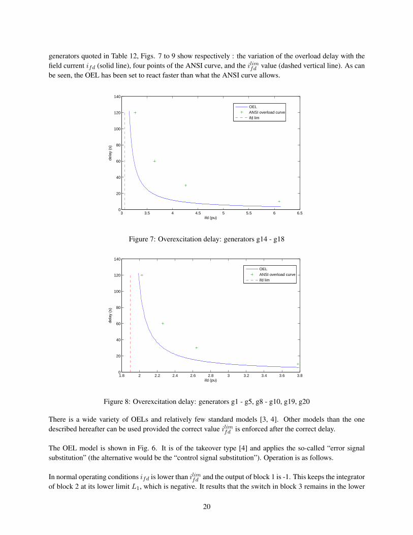
generators quoted in Table 12, Figs. 7 to 9 show respectively : the variation of the overload delay with thefield current ifd (solid line), four points of the ANSI curve, and the ilimfd value (dashed vertical line). As canbe seen, the OEL has been set to react faster than what the ANSI curve allows.
3 3.5 4 4.5 5 5.5 6 6.50
20
40
60
80
100
120
140
ifd (pu)
dela
y (s
)
OELANSI overload curveifd lim
Figure 7: Overexcitation delay: generators g14 - g18
1.8 2 2.2 2.4 2.6 2.8 3 3.2 3.4 3.6 3.80
20
40
60
80
100
120
140
ifd (pu)
dela
y (s
)
OELANSI overload curveifd lim
Figure 8: Overexcitation delay: generators g1 - g5, g8 - g10, g19, g20
There is a wide variety of OELs and relatively few standard models [3, 4]. Other models than the onedescribed hereafter can be used provided the correct value ilimfd is enforced after the correct delay.
The OEL model is shown in Fig. 6. It is of the takeover type [4] and applies the so-called “error signalsubstitution” (the alternative would be the “control signal substitution”). Operation is as follows.
In normal operating conditions ifd is lower than ilimfd and the output of block 1 is -1. This keeps the integratorof block 2 at its lower limit L1, which is negative. It results that the switch in block 3 remains in the lower
20
2.5 3 3.5 4 4.5 5 5.5 60
20
40
60
80
100
120
140
ifd (pu)
dela
y (s
)
OELANSI overload curveifdlim
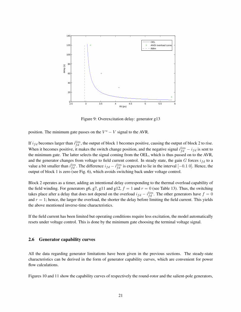
Figure 9: Overexcitation delay: generator g13
position. The minimum gate passes on the V o − V signal to the AVR.
If ifd becomes larger than ilimfd , the output of block 1 becomes positive, causing the output of block 2 to rise.When it becomes positive, it makes the switch change position, and the negative signal ilimfd − ifd is sent tothe minimum gate. The latter selects the signal coming from the OEL, which is thus passed on to the AVR,and the generator changes from voltage to field current control. In steady state, the gain G forces ifd to avalue a bit smaller than ilimfd . The difference ifd − ilimfd is expected to lie in the interval [−0.1 0]. Hence, theoutput of block 1 is zero (see Fig. 6), which avoids switching back under voltage control.
Block 2 operates as a timer, adding an intentional delay corresponding to the thermal overload capability ofthe field winding. For generators g6, g7, g11 and g12, f = 1 and r = 0 (see Table 13). Thus, the switchingtakes place after a delay that does not depend on the overload ifd − ilimfd . The other generators have f = 0
and r = 1; hence, the larger the overload, the shorter the delay before limiting the field current. This yieldsthe above mentioned inverse-time characteristics.
If the field current has been limited but operating conditions require less excitation, the model automaticallyresets under voltage control. This is done by the minimum gate choosing the terminal voltage signal.
2.6 Generator capability curves
All the data regarding generator limitations have been given in the previous sections. The steady-statecharacteristics can be derived in the form of generator capability curves, which are convenient for powerflow calculations.
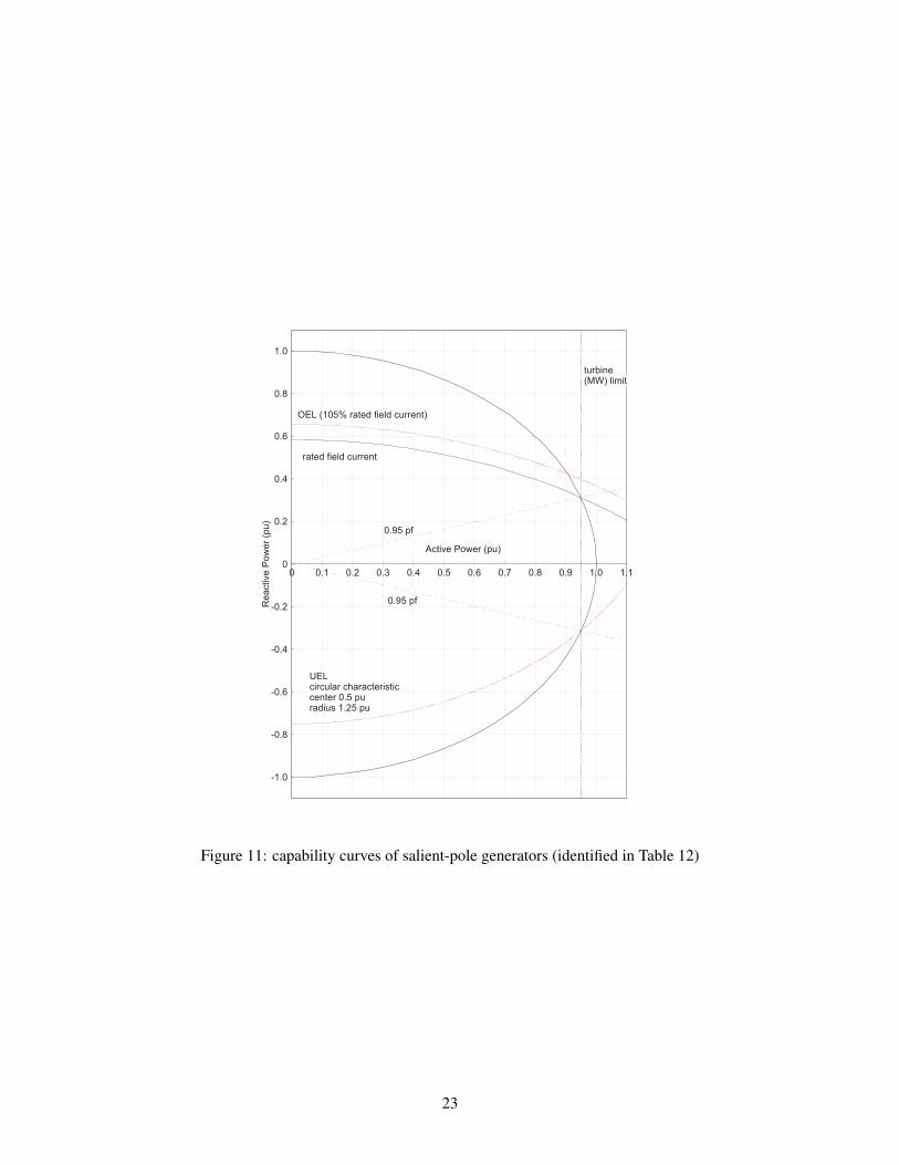
Figures 10 and 11 show the capability curves of respectively the round-rotor and the salient-pole generators,
21
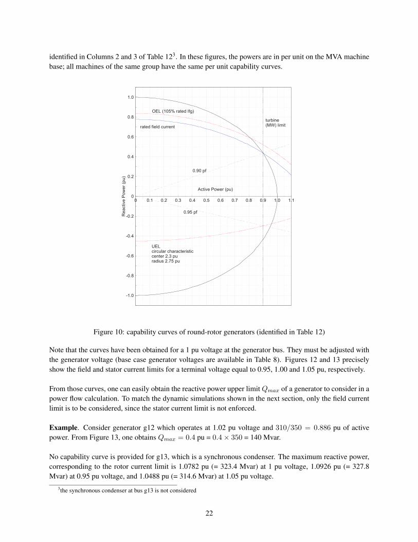
identified in Columns 2 and 3 of Table 123. In these figures, the powers are in per unit on the MVA machinebase; all machines of the same group have the same per unit capability curves.
-1.0
-0.8
-0.6
-0.4
-0.2
0
0.2
0.4
0.6
0.8
1.0
0 0.1 0.2 0.3 0.4 0.5 0.6 0.7 0.8 0.9 1.0 1.1
UELcircular characteristiccenter 2.3 puradius 2.75 pu
turbine(MW) limit
0.95 pf
0.90 pf
OEL (105% rated Ifg)
rated field current
Active Power (pu)
Re
active
Po
we
r (p
u)
Figure 10: capability curves of round-rotor generators (identified in Table 12)
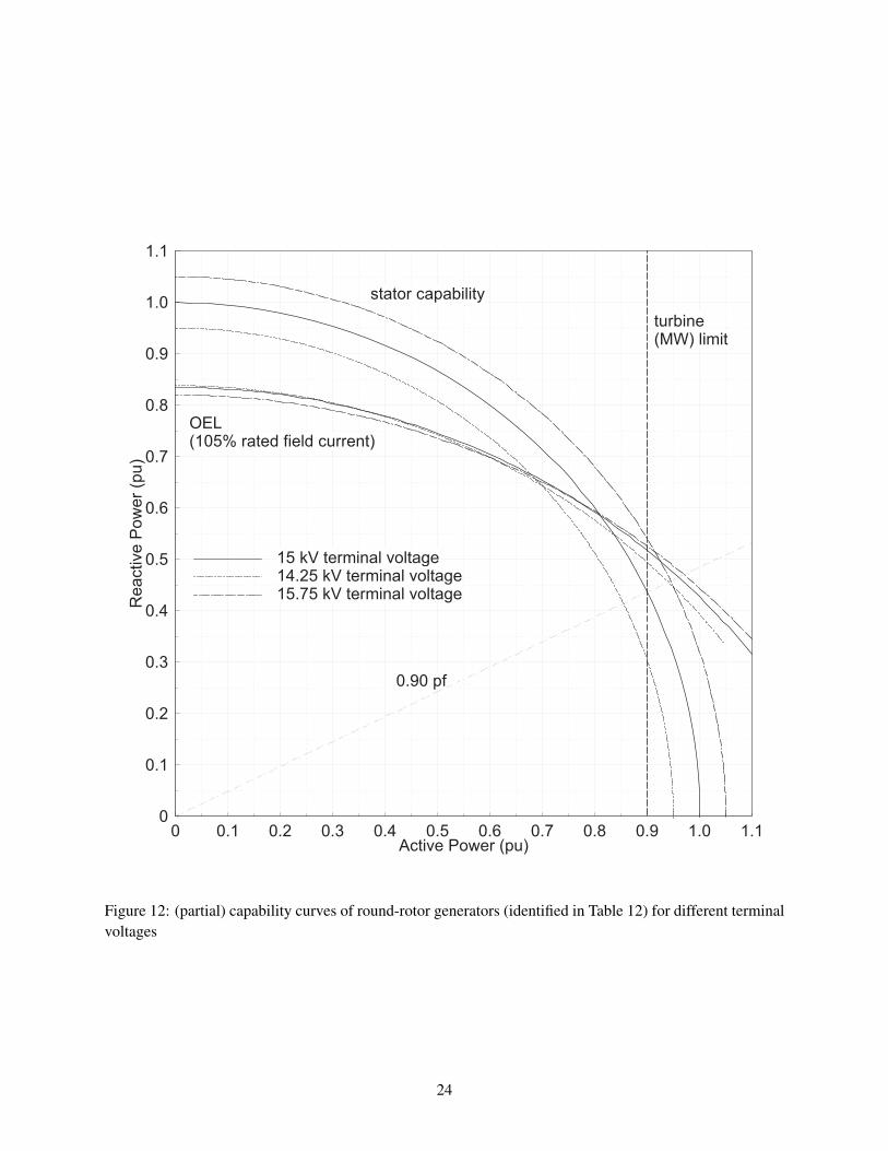
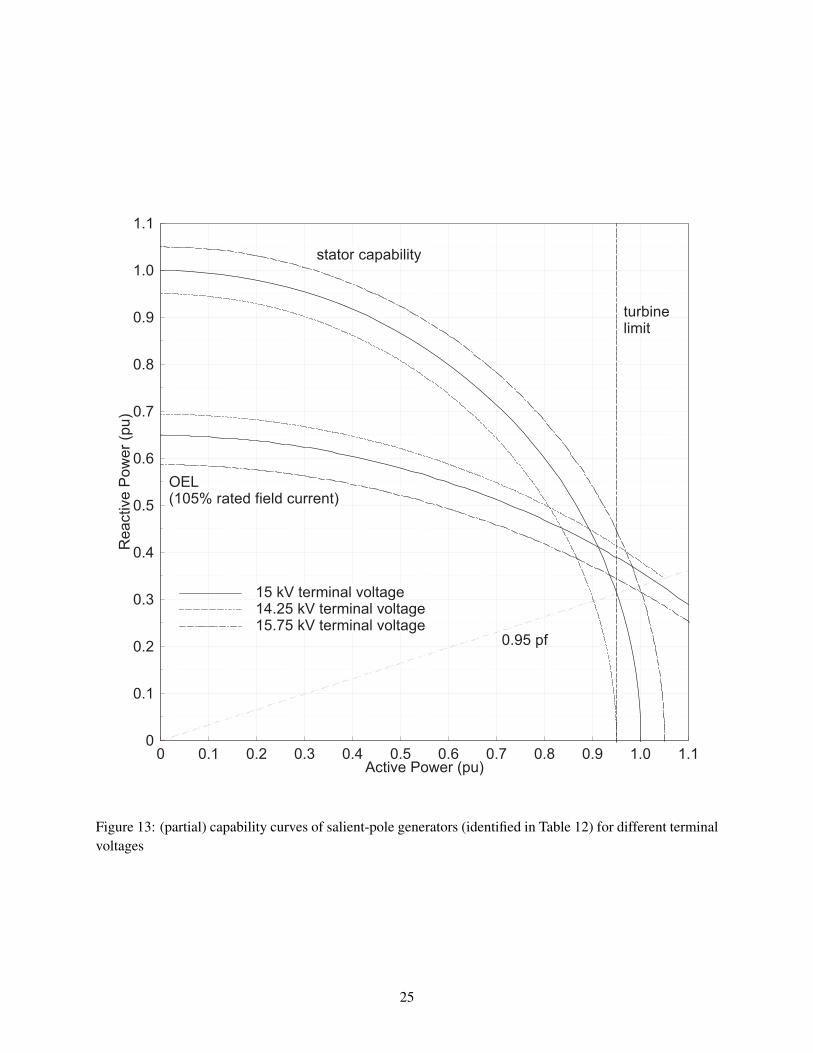
Note that the curves have been obtained for a 1 pu voltage at the generator bus. They must be adjusted withthe generator voltage (base case generator voltages are available in Table 8). Figures 12 and 13 preciselyshow the field and stator current limits for a terminal voltage equal to 0.95, 1.00 and 1.05 pu, respectively.
From those curves, one can easily obtain the reactive power upper limit Qmax of a generator to consider in apower flow calculation. To match the dynamic simulations shown in the next section, only the field currentlimit is to be considered, since the stator current limit is not enforced.
Example. Consider generator g12 which operates at 1.02 pu voltage and 310/350 = 0.886 pu of activepower. From Figure 13, one obtains Qmax = 0.4 pu = 0.4× 350 = 140 Mvar.
No capability curve is provided for g13, which is a synchronous condenser. The maximum reactive power,corresponding to the rotor current limit is 1.0782 pu (= 323.4 Mvar) at 1 pu voltage, 1.0926 pu (= 327.8Mvar) at 0.95 pu voltage, and 1.0488 pu (= 314.6 Mvar) at 1.05 pu voltage.
3the synchronous condenser at bus g13 is not considered
22
-1.0
-0.8
-0.6
-0.4
-0.2
0
0.2
0.4
0.6
0.8
1.0
0 0.1 0.2 0.3 0.4 0.5 0.6 0.7 0.8 0.9 1.0 1.1
turbine(MW) limit
OEL (105% rated field current)
rated field current
UELcircular characteristiccenter 0.5 puradius 1.25 pu
0.95 pf
0.95 pf
Active Power (pu)
Re
active
Po
we
r (p
u)
Figure 11: capability curves of salient-pole generators (identified in Table 12)
23
0
0.1
0.2
0.3
0.4
0.5
0.6
0.7
0.8
0.9
1.0
1.1
0 0.1 0.2 0.3 0.4 0.5 0.6 0.7 0.8 0.9 1.0 1.1
15 kV terminal voltage14.25 kV terminal voltage15.75 kV terminal voltage
turbine(MW) limit
stator capability
OEL(105% rated field current)
0.90 pf
Active Power (pu)
Re
active
Po
we
r (p
u)
Figure 12: (partial) capability curves of round-rotor generators (identified in Table 12) for different terminalvoltages
24
0
0.1
0.2
0.3
0.4
0.5
0.6
0.7
0.8
0.9
1.0
1.1
0 0.1 0.2 0.3 0.4 0.5 0.6 0.7 0.8 0.9 1.0 1.1
15 kV terminal voltage14.25 kV terminal voltage15.75 kV terminal voltage
0.95 pf
turbinelimit
stator capability
OEL(105% rated field current)
Active Power (pu)
Re
active
Po
we
r (p
u)
Figure 13: (partial) capability curves of salient-pole generators (identified in Table 12) for different terminalvoltages
25
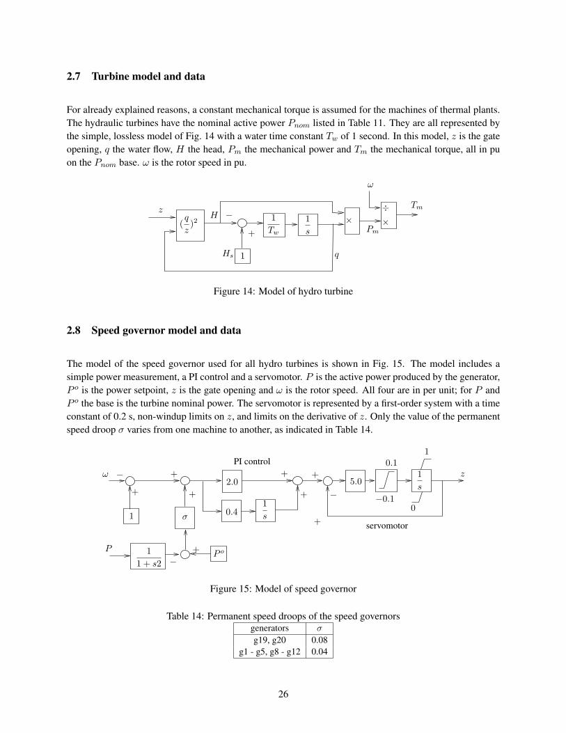
2.7 Turbine model and data
For already explained reasons, a constant mechanical torque is assumed for the machines of thermal plants.The hydraulic turbines have the nominal active power Pnom listed in Table 11. They are all represented bythe simple, lossless model of Fig. 14 with a water time constant Tw of 1 second. In this model, z is the gateopening, q the water flow, H the head, Pm the mechanical power and Tm the mechanical torque, all in puon the Pnom base. ω is the rotor speed in pu.
+
−Pm
(q
z)2
H
Hs
1
Tw
×z
q
×÷ Tm
ω
1
1
s
Figure 14: Model of hydro turbine
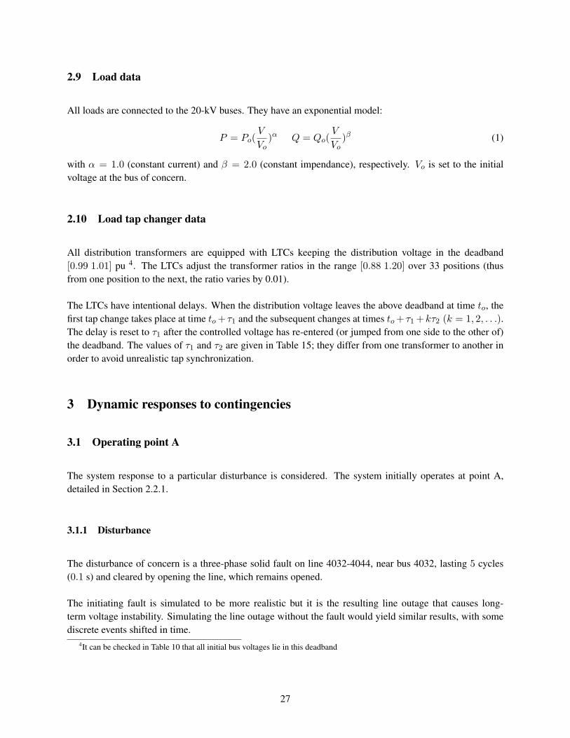
2.8 Speed governor model and data
The model of the speed governor used for all hydro turbines is shown in Fig. 15. The model includes asimple power measurement, a PI control and a servomotor. P is the active power produced by the generator,P o is the power setpoint, z is the gate opening and ω is the rotor speed. All four are in per unit; for P andP o the base is the turbine nominal power. The servomotor is represented by a first-order system with a timeconstant of 0.2 s, non-windup limits on z, and limits on the derivative of z. Only the value of the permanentspeed droop σ varies from one machine to another, as indicated in Table 14.
1 σ
P o1
1 + s2
+
5.02.0
servomotor
PI control+
+
+
−
z0.1
−0.1
1
0
1
s
+
+
0.4
ω −
1
s
P +
−
+
Figure 15: Model of speed governor
Table 14: Permanent speed droops of the speed governorsgenerators σ
g19, g20 0.08g1 - g5, g8 - g12 0.04
26
2.9 Load data
All loads are connected to the 20-kV buses. They have an exponential model:
P = Po(V
Vo)α Q = Qo(
V
Vo)β (1)
with α = 1.0 (constant current) and β = 2.0 (constant impendance), respectively. Vo is set to the initialvoltage at the bus of concern.
2.10 Load tap changer data
All distribution transformers are equipped with LTCs keeping the distribution voltage in the deadband[0.99 1.01] pu 4. The LTCs adjust the transformer ratios in the range [0.88 1.20] over 33 positions (thusfrom one position to the next, the ratio varies by 0.01).
The LTCs have intentional delays. When the distribution voltage leaves the above deadband at time to, thefirst tap change takes place at time to+ τ1 and the subsequent changes at times to+ τ1+kτ2 (k = 1, 2, . . .).The delay is reset to τ1 after the controlled voltage has re-entered (or jumped from one side to the other of)the deadband. The values of τ1 and τ2 are given in Table 15; they differ from one transformer to another inorder to avoid unrealistic tap synchronization.
3 Dynamic responses to contingencies
3.1 Operating point A
The system response to a particular disturbance is considered. The system initially operates at point A,detailed in Section 2.2.1.
3.1.1 Disturbance
The disturbance of concern is a three-phase solid fault on line 4032-4044, near bus 4032, lasting 5 cycles(0.1 s) and cleared by opening the line, which remains opened.
The initiating fault is simulated to be more realistic but it is the resulting line outage that causes long-term voltage instability. Simulating the line outage without the fault would yield similar results, with somediscrete events shifted in time.
4It can be checked in Table 10 that all initial bus voltages lie in this deadband
27
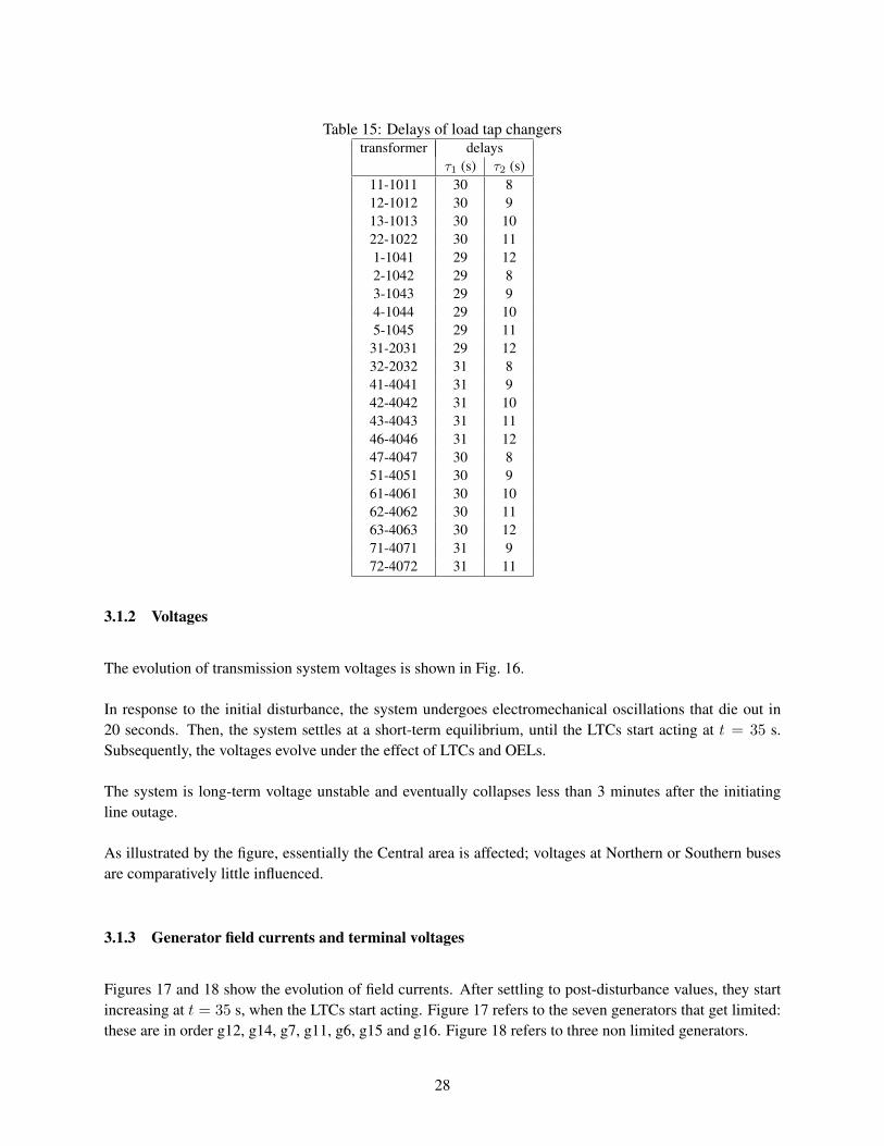
Table 15: Delays of load tap changerstransformer delays
τ1 (s) τ2 (s)11-1011 30 812-1012 30 913-1013 30 1022-1022 30 111-1041 29 122-1042 29 83-1043 29 94-1044 29 105-1045 29 1131-2031 29 1232-2032 31 841-4041 31 942-4042 31 1043-4043 31 1146-4046 31 1247-4047 30 851-4051 30 961-4061 30 1062-4062 30 1163-4063 30 1271-4071 31 972-4072 31 11
3.1.2 Voltages
The evolution of transmission system voltages is shown in Fig. 16.
In response to the initial disturbance, the system undergoes electromechanical oscillations that die out in20 seconds. Then, the system settles at a short-term equilibrium, until the LTCs start acting at t = 35 s.Subsequently, the voltages evolve under the effect of LTCs and OELs.
The system is long-term voltage unstable and eventually collapses less than 3 minutes after the initiatingline outage.
As illustrated by the figure, essentially the Central area is affected; voltages at Northern or Southern busesare comparatively little influenced.
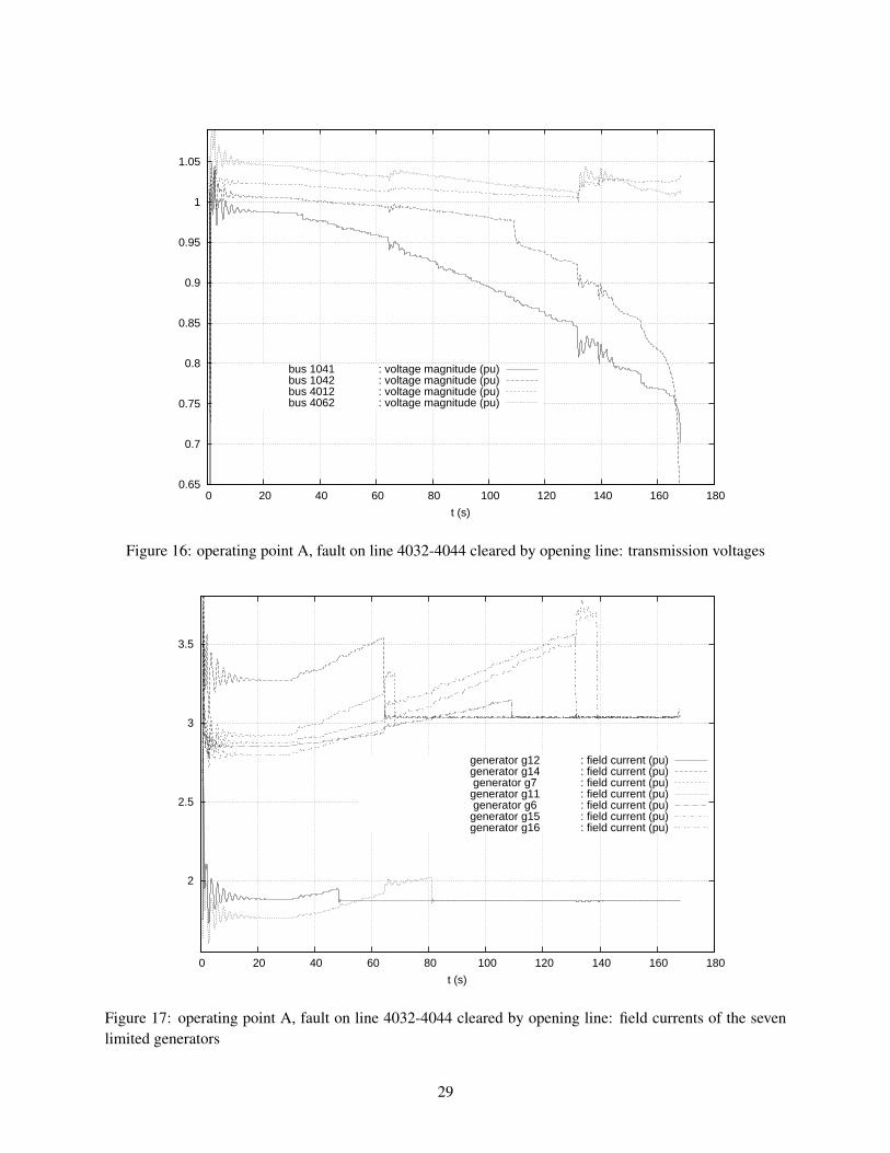
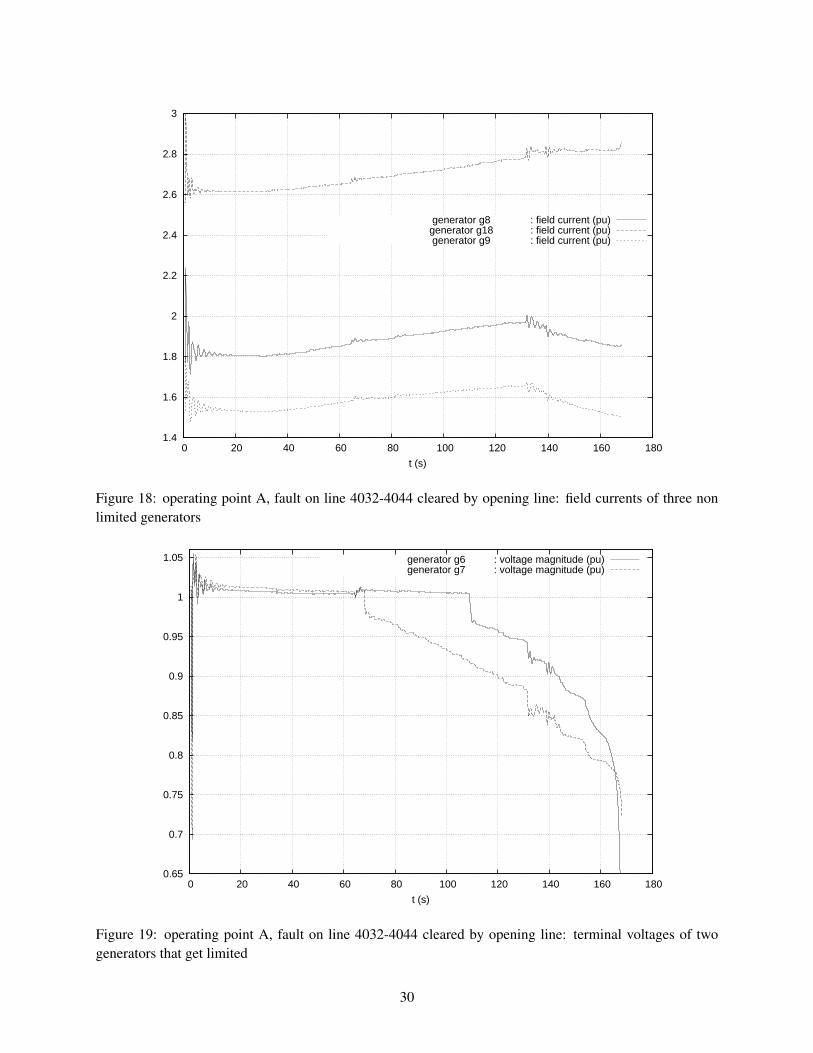
3.1.3 Generator field currents and terminal voltages
Figures 17 and 18 show the evolution of field currents. After settling to post-disturbance values, they startincreasing at t = 35 s, when the LTCs start acting. Figure 17 refers to the seven generators that get limited:these are in order g12, g14, g7, g11, g6, g15 and g16. Figure 18 refers to three non limited generators.
28
0.65
0.7
0.75
0.8
0.85
0.9
0.95
1
1.05
0 20 40 60 80 100 120 140 160 180
t (s)
bus 1041 : voltage magnitude (pu)bus 1042 : voltage magnitude (pu)bus 4012 : voltage magnitude (pu)bus 4062 : voltage magnitude (pu)
Figure 16: operating point A, fault on line 4032-4044 cleared by opening line: transmission voltages
2
2.5
3
3.5
0 20 40 60 80 100 120 140 160 180
t (s)
generator g12 : field current (pu)generator g14 : field current (pu)generator g7 : field current (pu)
generator g11 : field current (pu)generator g6 : field current (pu)
generator g15 : field current (pu)generator g16 : field current (pu)
Figure 17: operating point A, fault on line 4032-4044 cleared by opening line: field currents of the sevenlimited generators
29
1.4
1.6
1.8
2
2.2
2.4
2.6
2.8
3
0 20 40 60 80 100 120 140 160 180
t (s)
generator g8 : field current (pu)generator g18 : field current (pu)generator g9 : field current (pu)
Figure 18: operating point A, fault on line 4032-4044 cleared by opening line: field currents of three nonlimited generators
0.65
0.7
0.75
0.8
0.85
0.9
0.95
1
1.05
0 20 40 60 80 100 120 140 160 180
t (s)
generator g6 : voltage magnitude (pu)generator g7 : voltage magnitude (pu)
Figure 19: operating point A, fault on line 4032-4044 cleared by opening line: terminal voltages of twogenerators that get limited
30
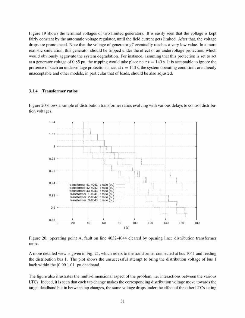
Figure 19 shows the terminal voltages of two limited generators. It is easily seen that the voltage is keptfairly constant by the automatic voltage regulator, until the field current gets limited. After that, the voltagedrops are pronounced. Note that the voltage of generator g7 eventually reaches a very low value. In a morerealistic simulation, this generator should be tripped under the effect of an undervoltage protection, whichwould obviously aggravate the system degradation. For instance, assuming that this protection is set to actat a generator voltage of 0.85 pu, the tripping would take place near t = 140 s. It is acceptable to ignore thepresence of such an undervoltage protection since, at t = 140 s, the system operating conditions are alreadyunacceptable and other models, in particular that of loads, should be also adjusted.
3.1.4 Transformer ratios
Figure 20 shows a sample of distribution transformer ratios evolving with various delays to control distribu-tion voltages.
0.88
0.9
0.92
0.94
0.96
0.98
1
1.02
1.04
0 20 40 60 80 100 120 140 160 180
t (s)
transformer 41-4041 : ratio (pu)transformer 42-4042 : ratio (pu)transformer 43-4043 : ratio (pu)transformer 1-1041 : ratio (pu)transformer 2-1042 : ratio (pu)transformer 3-1043 : ratio (pu)
Figure 20: operating point A, fault on line 4032-4044 cleared by opening line: distribution transformerratios
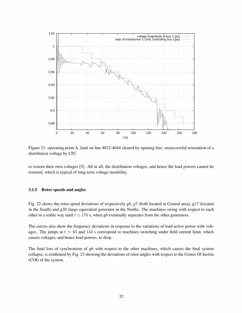
A more detailed view is given in Fig. 21, which refers to the transformer connected at bus 1041 and feedingthe distribution bus 1. The plot shows the unsuccessful attempt to bring the distribution voltage of bus 1back within the [0.99 1.01] pu deadband.
The figure also illustrates the multi-dimensional aspect of the problem, i.e. interactions between the variousLTCs. Indeed, it is seen that each tap change makes the corresponding distribution voltage move towards thetarget deadband but in between tap changes, the same voltage drops under the effect of the other LTCs acting
31
0.88
0.9
0.92
0.94
0.96
0.98
1
1.02
0 20 40 60 80 100 120 140 160 180
t (s)
voltage magnitude at bus 1 (pu)ratio of transformer 1-1041 controlling bus 1(pu)
Figure 21: operating point A, fault on line 4032-4044 cleared by opening line: unsuccessful restoration of adistribution voltage by LTC
to restore their own voltages [5]. All in all, the distribution voltages, and hence the load powers cannot berestored, which is typical of long-term voltage instability.
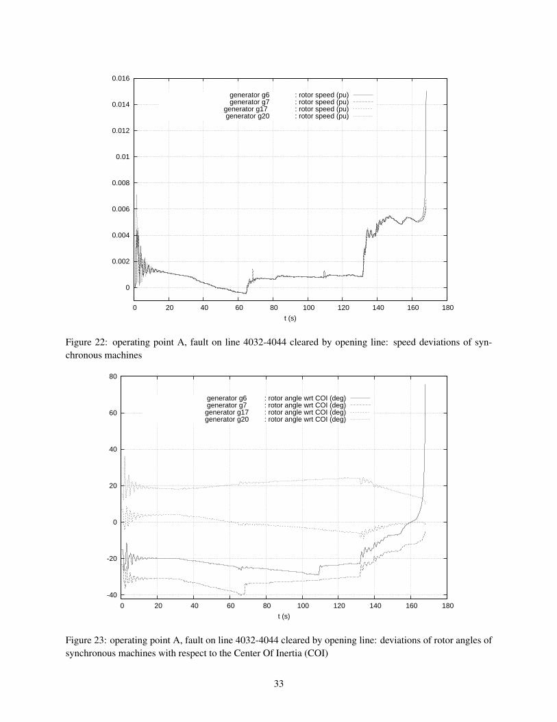
3.1.5 Rotor speeds and angles
Fig. 22 shows the rotor speed deviations of respectively g6, g7 (both located in Central area), g17 (locatedin the South) and g20 (large equivalent generator in the North). The machines swing with respect to eachother in a stable way until t ≃ 170 s, when g6 eventually separates from the other generators.
The curves also show the frequency deviations in response to the variations of load active power with volt-ages. The jumps at t ≃ 65 and 132 s correspond to machines switching under field current limit, whichcauses voltages, and hence load powers, to drop.
The final loss of synchronism of g6 with respect to the other machines, which causes the final systemcollapse, is confirmed by Fig. 23 showing the deviations of rotor angles with respect to the Center Of Inertia(COI) of the system.
32
0
0.002
0.004
0.006
0.008
0.01
0.012
0.014
0.016
0 20 40 60 80 100 120 140 160 180
t (s)
generator g6 : rotor speed (pu)generator g7 : rotor speed (pu)
generator g17 : rotor speed (pu)generator g20 : rotor speed (pu)
Figure 22: operating point A, fault on line 4032-4044 cleared by opening line: speed deviations of syn-chronous machines
-40
-20
0
20
40
60
80
0 20 40 60 80 100 120 140 160 180
t (s)
generator g6 : rotor angle wrt COI (deg)generator g7 : rotor angle wrt COI (deg)
generator g17 : rotor angle wrt COI (deg)generator g20 : rotor angle wrt COI (deg)
Figure 23: operating point A, fault on line 4032-4044 cleared by opening line: deviations of rotor angles ofsynchronous machines with respect to the Center Of Inertia (COI)
33
3.2 Operating point B
At this operating point, an exhaustive contingency analysis has been performed using time simulation.
The following contingencies have been considered:
• a 5-cycle (0.1 s) fault on any line, cleared by tripping the line;
• the outage of any single generator, except g19 and g20, which are equivalent generators. This includesthe outage of one among the generators: g15, g15b, g16, g16b, g18 and g18b5.
The post-contingency evolution has been considered acceptable if, over a simulation interval of 600 seconds:
• all distribution bus voltages are restored in their [0.99 1.01] pu deadbands;
• no generator has its terminal voltage falling below 0.85 pu, except possibly for the fault-on period;
• no loss of synchronism takes place.
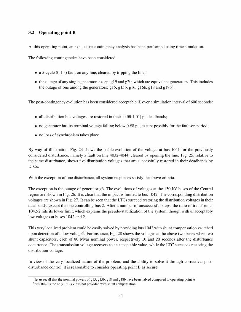
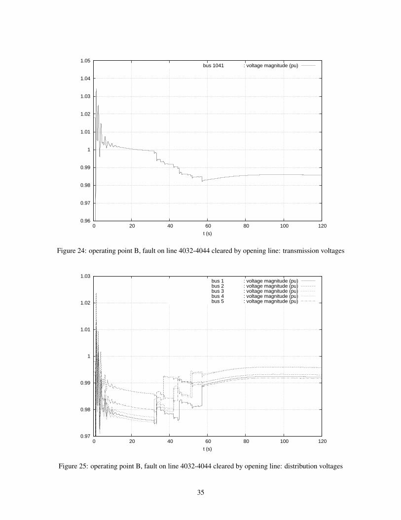
By way of illustration, Fig. 24 shows the stable evolution of the voltage at bus 1041 for the previouslyconsidered disturbance, namely a fault on line 4032-4044, cleared by opening the line. Fig. 25, relative tothe same disturbance, shows five distribution voltages that are successfully restored in their deadbands byLTCs.
With the exception of one disturbance, all system responses satisfy the above criteria.
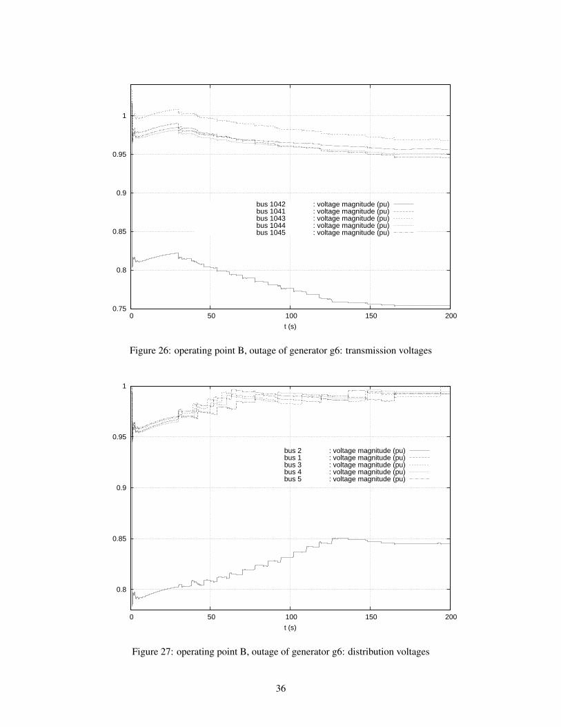
The exception is the outage of generator g6. The evolutions of voltages at the 130-kV buses of the Centralregion are shown in Fig. 26. It is clear that the impact is limited to bus 1042. The corresponding distributionvoltages are shown in Fig. 27. It can be seen that the LTCs succeed restoring the distribution voltages in theirdeadbands, except the one controlling bus 2. After a number of unsuccessful steps, the ratio of transformer1042-2 hits its lower limit, which explains the pseudo-stabilization of the system, though with unacceptablylow voltages at buses 1042 and 2.
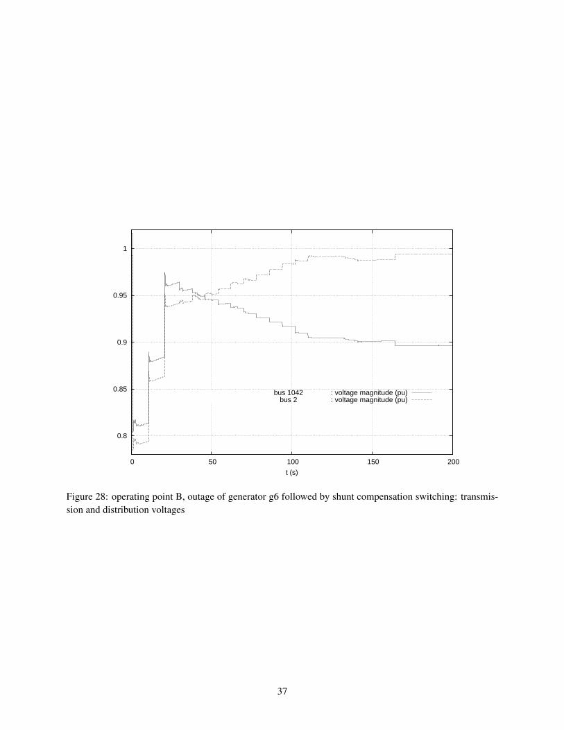
This very localized problem could be easily solved by providing bus 1042 with shunt compensation switchedupon detection of a low voltage6. For instance, Fig. 28 shows the voltages at the above two buses when twoshunt capacitors, each of 80 Mvar nominal power, respectively 10 and 20 seconds after the disturbanceoccurrence. The transmission voltage recovers to an acceptable value, while the LTC succeeds restoring thedistribution voltage.
In view of the very localized nature of the problem, and the ability to solve it through corrective, post-disturbance control, it is reasonable to consider operating point B as secure.
5let us recall that the nominal powers of g15, g15b, g18 and g18b have been halved compared to operating point A6bus 1042 is the only 130-kV bus not provided with shunt compensation
34
0.96
0.97
0.98
0.99
1
1.01
1.02
1.03
1.04
1.05
0 20 40 60 80 100 120
t (s)
bus 1041 : voltage magnitude (pu)
Figure 24: operating point B, fault on line 4032-4044 cleared by opening line: transmission voltages
0.97
0.98
0.99
1
1.01
1.02
1.03
0 20 40 60 80 100 120
t (s)
bus 1 : voltage magnitude (pu)bus 2 : voltage magnitude (pu)bus 3 : voltage magnitude (pu)bus 4 : voltage magnitude (pu)bus 5 : voltage magnitude (pu)
Figure 25: operating point B, fault on line 4032-4044 cleared by opening line: distribution voltages
35
0.75
0.8
0.85
0.9
0.95
1
0 50 100 150 200
t (s)
bus 1042 : voltage magnitude (pu)bus 1041 : voltage magnitude (pu)bus 1043 : voltage magnitude (pu)bus 1044 : voltage magnitude (pu)bus 1045 : voltage magnitude (pu)
Figure 26: operating point B, outage of generator g6: transmission voltages
0.8
0.85
0.9
0.95
1
0 50 100 150 200
t (s)
bus 2 : voltage magnitude (pu)bus 1 : voltage magnitude (pu)bus 3 : voltage magnitude (pu)bus 4 : voltage magnitude (pu)bus 5 : voltage magnitude (pu)
Figure 27: operating point B, outage of generator g6: distribution voltages
36
0.8
0.85
0.9
0.95
1
0 50 100 150 200
t (s)
bus 1042 : voltage magnitude (pu)bus 2 : voltage magnitude (pu)
Figure 28: operating point B, outage of generator g6 followed by shunt compensation switching: transmis-sion and distribution voltages
37
4 Examples of preventive security margin computations
This section is devoted to the determination of Secure Operation Limits (SOL) and power margins for thesystem operating at point B.
4.1 Secure operation limit: definition
An SOL involves stressing the system in its pre-contingency configuration. The stress considered here is anincrease of loads in the Central area.
The SOL corresponds to the maximum load power that can be accepted in the pre-contingency configurationsuch that the system responds in a stable way to each of the specified contingencies [4].
To this purpose, power flow computations are performed for increasing values of the Central active andreactive loads. For each so determined operating point, the disturbance is simulated and the system responseis analyzed.
In all cases, the criteria that lead to accepting the system response are those detailed in Section 3.2.
4.2 Pre-contingency stress
The Central area load is increased by steps of 25 MW. The total active power variation is shared by the11 loads present in this area, in proportion to their base case value. The power factor of each load is keptconstant. The active power variations are compensated by generator g20, taken as slack-bus.
In the pre-contingency power flow calculations, transformer ratios are adjusted in response to load changesas follows:
1. the 22 distribution transformers are adjusted in order to maintain the distribution voltages in the dead-bands as previously described;
2. the 400/130-kV transformers 1044-4044, 1044-4044b, 1045-4045 and 1045-4045b are assumed tobe controlled by operators, adjusting their ratio to maintain the voltages at buses 1044 and 1045in deadbands. Note that these transformers do not have their tap changed in the post-disturbancesimulation, whose duration is considered too short for operators to react.
In both cases, ratios are modified when the controlled voltages leave their deadbands, and vary in discretesteps. The ratios of transformers in parallel are varied together.
The data of the distribution transformers have been given in Section 2.10, while Table 16 gives the datarelative to the 400/130 kV transformers.
38
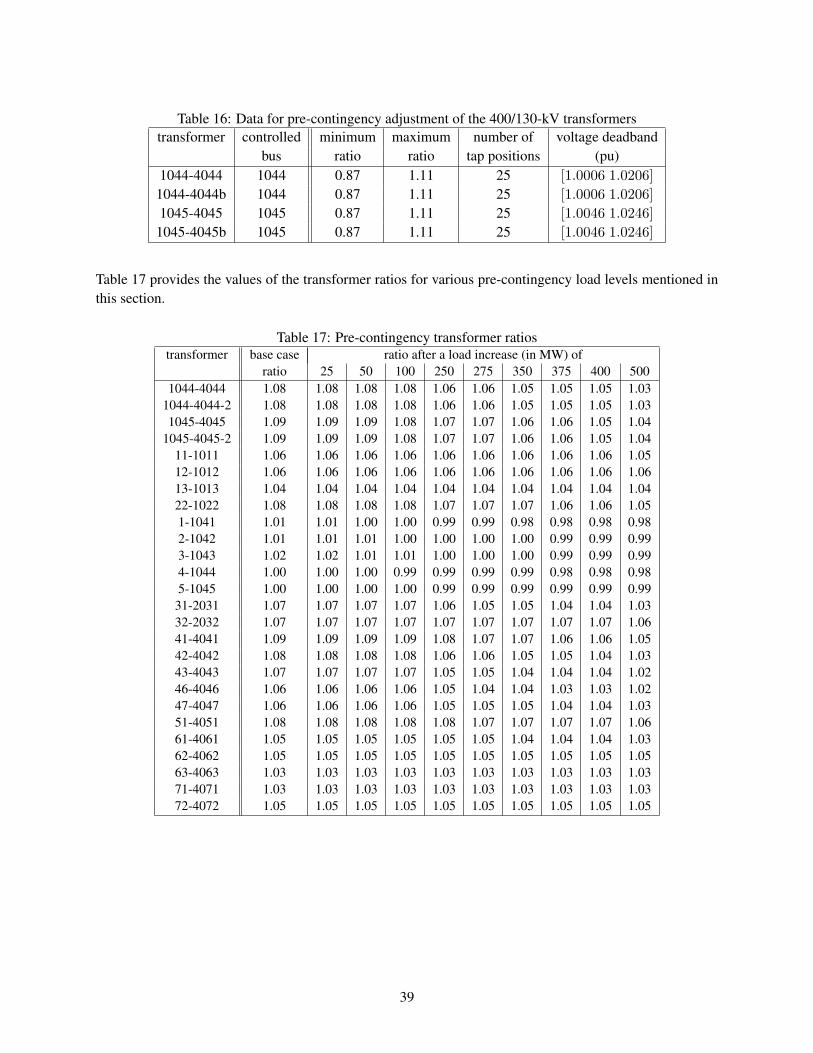
Table 16: Data for pre-contingency adjustment of the 400/130-kV transformerstransformer controlled minimum maximum number of voltage deadband
bus ratio ratio tap positions (pu)1044-4044 1044 0.87 1.11 25 [1.0006 1.0206]
1044-4044b 1044 0.87 1.11 25 [1.0006 1.0206]
1045-4045 1045 0.87 1.11 25 [1.0046 1.0246]
1045-4045b 1045 0.87 1.11 25 [1.0046 1.0246]
Table 17 provides the values of the transformer ratios for various pre-contingency load levels mentioned inthis section.
Table 17: Pre-contingency transformer ratiostransformer base case ratio after a load increase (in MW) of
ratio 25 50 100 250 275 350 375 400 5001044-4044 1.08 1.08 1.08 1.08 1.06 1.06 1.05 1.05 1.05 1.03
1044-4044-2 1.08 1.08 1.08 1.08 1.06 1.06 1.05 1.05 1.05 1.031045-4045 1.09 1.09 1.09 1.08 1.07 1.07 1.06 1.06 1.05 1.04
1045-4045-2 1.09 1.09 1.09 1.08 1.07 1.07 1.06 1.06 1.05 1.0411-1011 1.06 1.06 1.06 1.06 1.06 1.06 1.06 1.06 1.06 1.0512-1012 1.06 1.06 1.06 1.06 1.06 1.06 1.06 1.06 1.06 1.0613-1013 1.04 1.04 1.04 1.04 1.04 1.04 1.04 1.04 1.04 1.0422-1022 1.08 1.08 1.08 1.08 1.07 1.07 1.07 1.06 1.06 1.051-1041 1.01 1.01 1.00 1.00 0.99 0.99 0.98 0.98 0.98 0.982-1042 1.01 1.01 1.01 1.00 1.00 1.00 1.00 0.99 0.99 0.993-1043 1.02 1.02 1.01 1.01 1.00 1.00 1.00 0.99 0.99 0.994-1044 1.00 1.00 1.00 0.99 0.99 0.99 0.99 0.98 0.98 0.985-1045 1.00 1.00 1.00 1.00 0.99 0.99 0.99 0.99 0.99 0.9931-2031 1.07 1.07 1.07 1.07 1.06 1.05 1.05 1.04 1.04 1.0332-2032 1.07 1.07 1.07 1.07 1.07 1.07 1.07 1.07 1.07 1.0641-4041 1.09 1.09 1.09 1.09 1.08 1.07 1.07 1.06 1.06 1.0542-4042 1.08 1.08 1.08 1.08 1.06 1.06 1.05 1.05 1.04 1.0343-4043 1.07 1.07 1.07 1.07 1.05 1.05 1.04 1.04 1.04 1.0246-4046 1.06 1.06 1.06 1.06 1.05 1.04 1.04 1.03 1.03 1.0247-4047 1.06 1.06 1.06 1.06 1.05 1.05 1.05 1.04 1.04 1.0351-4051 1.08 1.08 1.08 1.08 1.08 1.07 1.07 1.07 1.07 1.0661-4061 1.05 1.05 1.05 1.05 1.05 1.05 1.04 1.04 1.04 1.0362-4062 1.05 1.05 1.05 1.05 1.05 1.05 1.05 1.05 1.05 1.0563-4063 1.03 1.03 1.03 1.03 1.03 1.03 1.03 1.03 1.03 1.0371-4071 1.03 1.03 1.03 1.03 1.03 1.03 1.03 1.03 1.03 1.0372-4072 1.05 1.05 1.05 1.05 1.05 1.05 1.05 1.05 1.05 1.05
39
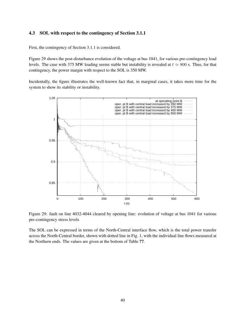
4.3 SOL with respect to the contingency of Section 3.1.1
First, the contingency of Section 3.1.1 is considered.
Figure 29 shows the post-disturbance evolution of the voltage at bus 1041, for various pre-contingency loadlevels. The case with 375 MW loading seems stable but instability is revealed at t ≃ 800 s. Thus, for thatcontingency, the power margin with respect to the SOL is 350 MW.
Incidentally, the figure illustrates the well-known fact that, in marginal cases, it takes more time for thesystem to show its stability or instability.
0.85
0.9
0.95
1
1.05
0 100 200 300 400 500 600
t (s)
at operating point Boper. pt B with central load increased by 350 MWoper. pt B with central load increased by 375 MWoper. pt B with central load increased by 400 MWoper. pt B with central load increased by 500 MW
Figure 29: fault on line 4032-4044 cleared by opening line: evolution of voltage at bus 1041 for variouspre-contingency stress levels
The SOL can be expressed in terms of the North-Central interface flow, which is the total power transferacross the North-Central border, shown with dotted line in Fig. 1, with the individual line flows measured atthe Northern ends. The values are given at the bottom of Table ??.
40
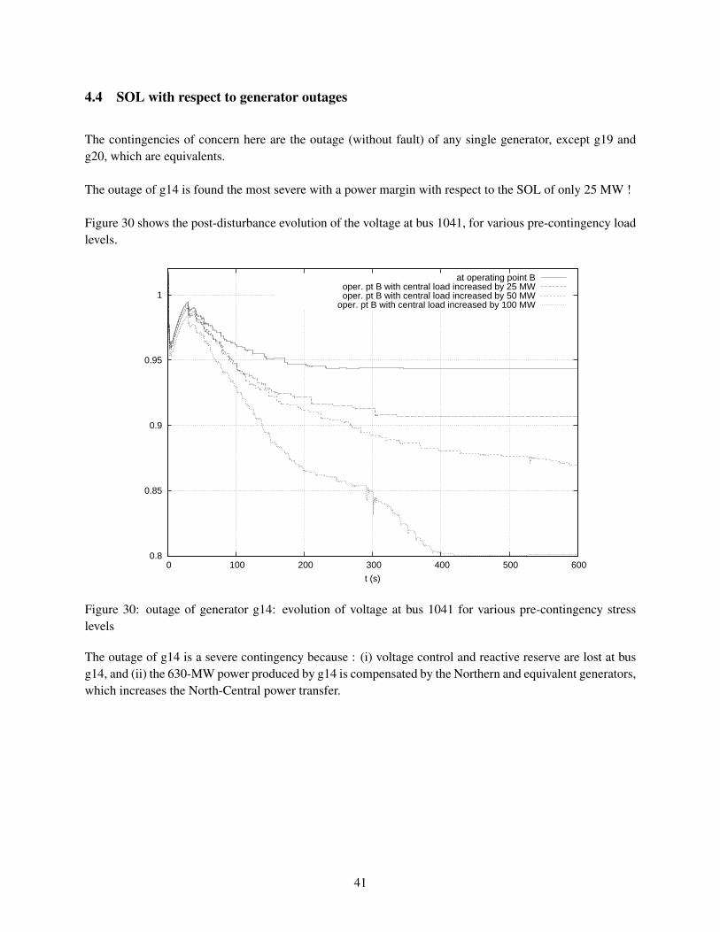
4.4 SOL with respect to generator outages
The contingencies of concern here are the outage (without fault) of any single generator, except g19 andg20, which are equivalents.
The outage of g14 is found the most severe with a power margin with respect to the SOL of only 25 MW !
Figure 30 shows the post-disturbance evolution of the voltage at bus 1041, for various pre-contingency loadlevels.
0.8
0.85
0.9
0.95
1
0 100 200 300 400 500 600
t (s)
at operating point Boper. pt B with central load increased by 25 MWoper. pt B with central load increased by 50 MW
oper. pt B with central load increased by 100 MW
Figure 30: outage of generator g14: evolution of voltage at bus 1041 for various pre-contingency stresslevels
The outage of g14 is a severe contingency because : (i) voltage control and reactive reserve are lost at busg14, and (ii) the 630-MW power produced by g14 is compensated by the Northern and equivalent generators,which increases the North-Central power transfer.
41
4.5 SOL with respect to line outages
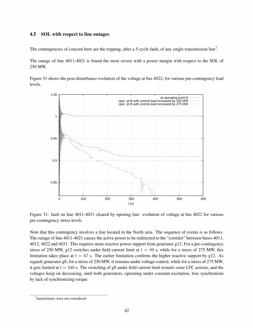
The contingencies of concern here are the tripping, after a 5-cycle fault, of any single transmission line7.
The outage of line 4011-4021 is found the most severe with a power margin with respect to the SOL of250 MW.
Figure 31 shows the post-disturbance evolution of the voltage at bus 4022, for various pre-contingency loadlevels.
0.85
0.9
0.95
1
1.05
0 100 200 300 400 500 600
t (s)
at operating point Boper. pt B with central load increased by 250 MWoper. pt B with central load increased by 275 MW
Figure 31: fault on line 4011-4021 cleared by opening line: evolution of voltage at bus 4022 for variouspre-contingency stress levels
Note that this contingency involves a line located in the North area. The sequence of events is as follows.The outage of line 4011-4021 causes the active power to be redirected to the “corridor” between buses 4011,4012, 4022 and 4031. This requires more reactive power support from generator g12. For a pre-contingencystress of 250 MW, g12 switches under field current limit at t = 89 s, while for a stress of 275 MW, thislimitation takes place at t = 67 s. The earlier limitation confirms the higher reactive support by g12. Asregards generator g8, for a stress of 250 MW, it remains under voltage control, while for a stress of 275 MW,it gets limited at t = 340 s. The switching of g8 under field current limit restarts some LTC actions, and thevoltages keep on decreasing, until both generators, operating under constant excitation, lose synchronismby lack of synchronizing torque.
7transformers were not considered
42
5 Examples of corrective post-disturbance control
5.1 Modified tap changer control
This section and the next one illustrate emergency control actions, typical of System Integrity ProtectionScheme (SIPS). Note that the material does not intend to be an exhaustive investigation of emergency con-trols; neither have these controls been “optimized” (for instance to minimize customer inconvenience).
The emergency control example consists of decreasing by 0.05 pu the voltage setpoint of LTCs controllingloads. This exploits the sensitivity of load power to voltage. For active power, with a constant current charac-teristic, one can expect a 5 % reduction, while for reactive power, with a constant impedance characteristic,one can expect a 10 % reduction.
Although many variants can be thought of, in the considered scenario the action is applied at t = 100 s, alittle after the lowest transmission voltage (at bus 1041) has reached 0.90 pu. Two sets of LTCs have beenconsidered:
• the five LTCs controlling loads at buses 1, 2, 3, 4 and 5;
• the same together with the six LTCs controlling loads at buses 41, 42, 43, 46, 47 and 51.
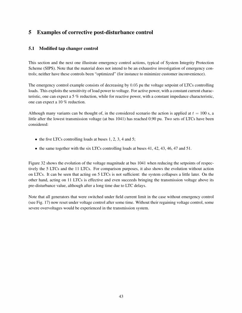
Figure 32 shows the evolution of the voltage magnitude at bus 1041 when reducing the setpoints of respec-tively the 5 LTCs and the 11 LTCs. For comparison purposes, it also shows the evolution without actionon LTCs. It can be seen that acting on 5 LTCs is not sufficient: the system collapses a little later. On theother hand, acting on 11 LTCs is effective and even succeeds bringing the transmission voltage above itspre-disturbance value, although after a long time due to LTC delays.
Note that all generators that were switched under field current limit in the case without emergency control(see Fig. 17) now reset under voltage control after some time. Without their regaining voltage control, somesevere overvoltages would be experienced in the transmission system.
43
0.7
0.75
0.8
0.85
0.9
0.95
1
1.05
0 100 200 300 400 500 600
t (s)
no action on LTCsvolt. setpoint reduction on 5 LTCs
volt. setpoint reduction on 11 LTCs
Figure 32: Evolution of voltage magnitude at bus 1041, without and with emergency control of LTCs
44
5.2 Undervoltage load shedding
The second example of emergency control deals with undervoltage load shedding. Distributed controllershave been considered as detailed in [7]. Each controller monitors the voltage at a transmission bus and actson the load at the nearest distribution bus, according to the following simple logic:
shed ∆P MW of load when the monitored voltage V goes below a threshold V th for more thanτ seconds.
Important features are the ability of each controller to act several times (a closed-loop behaviour that yieldsa robust and adaptive protection) and the absence of communication between controllers.
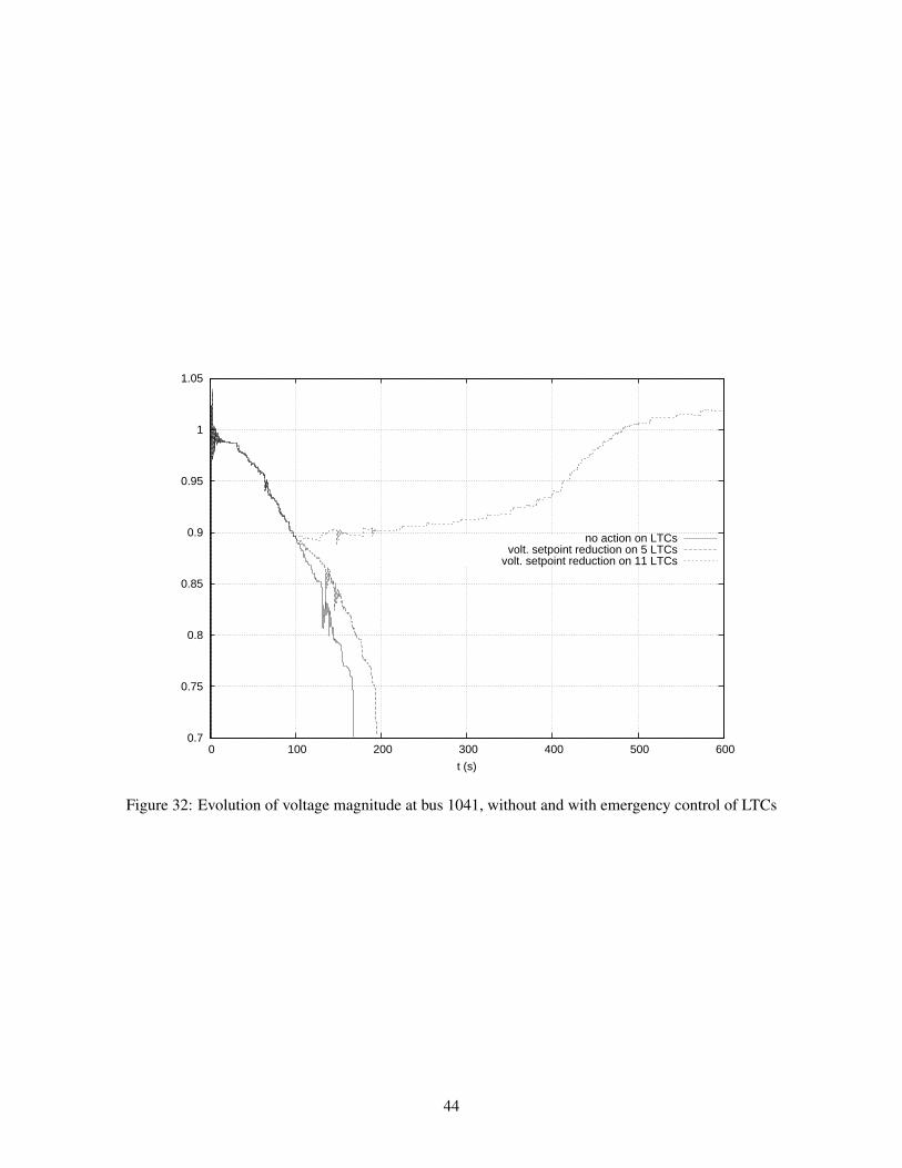
The example given hereafter has been obtained with V th = 0.90 pu, ∆P = 50 MW, and τ = 3 seconds.Each time a block is shed, the value of Po in (1) is decreased by ∆P and Qo by ∆Q.∆Q has been chosenso that the load power factor at 1 pu voltage is preserved.
Figure 33 shows the performance of the so adjusted load shedding controllers. Six blocks of load are shed,two by the controller monitoring bus 1041 and acting on bus 1 (at t = 100 and 144.95 s) and four by thecontroller of monitoring bus 1044 and acting on bus 4 (at t = 112.10, 123.10, 180.40 and 290.45 s), for atotal of 300 MW.
0.86
0.88
0.9
0.92
0.94
0.96
0.98
1
1.02
0 50 100 150 200 250
t (s)
voltage magnitude at bus 1041 (pu) with load sheddingvoltage magnitude at bus 1041 (pu) without load shedding
Figure 33: Evolution of voltage magnitude at bus 1041, without and with load shedding
45
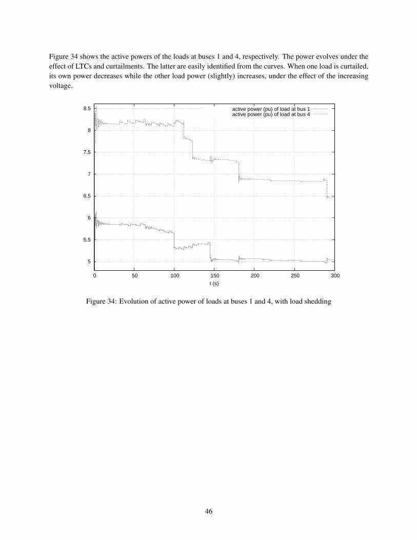
Figure 34 shows the active powers of the loads at buses 1 and 4, respectively. The power evolves under theeffect of LTCs and curtailments. The latter are easily identified from the curves. When one load is curtailed,its own power decreases while the other load power (slightly) increases, under the effect of the increasingvoltage.
5
5.5
6
6.5
7
7.5
8
8.5
0 50 100 150 200 250 300
t (s)
active power (pu) of load at bus 1active power (pu) of load at bus 4
Figure 34: Evolution of active power of loads at buses 1 and 4, with load shedding
46
6 Long-term voltage instability analysis through sensitivities
Long-term voltage instability results from the attempt of loads to restore their powers at a level that thecombined transmission and generation systems cannot provide [4]. In this test system, as in many real-lifesystems, load power restoration comes from the LTCs which try to restore load voltages. At the same time,the system weakening caused by the line outage reduces the maximum power that can be delivered to loads,while the reactive power limits of generators contribute to further reducing this power.
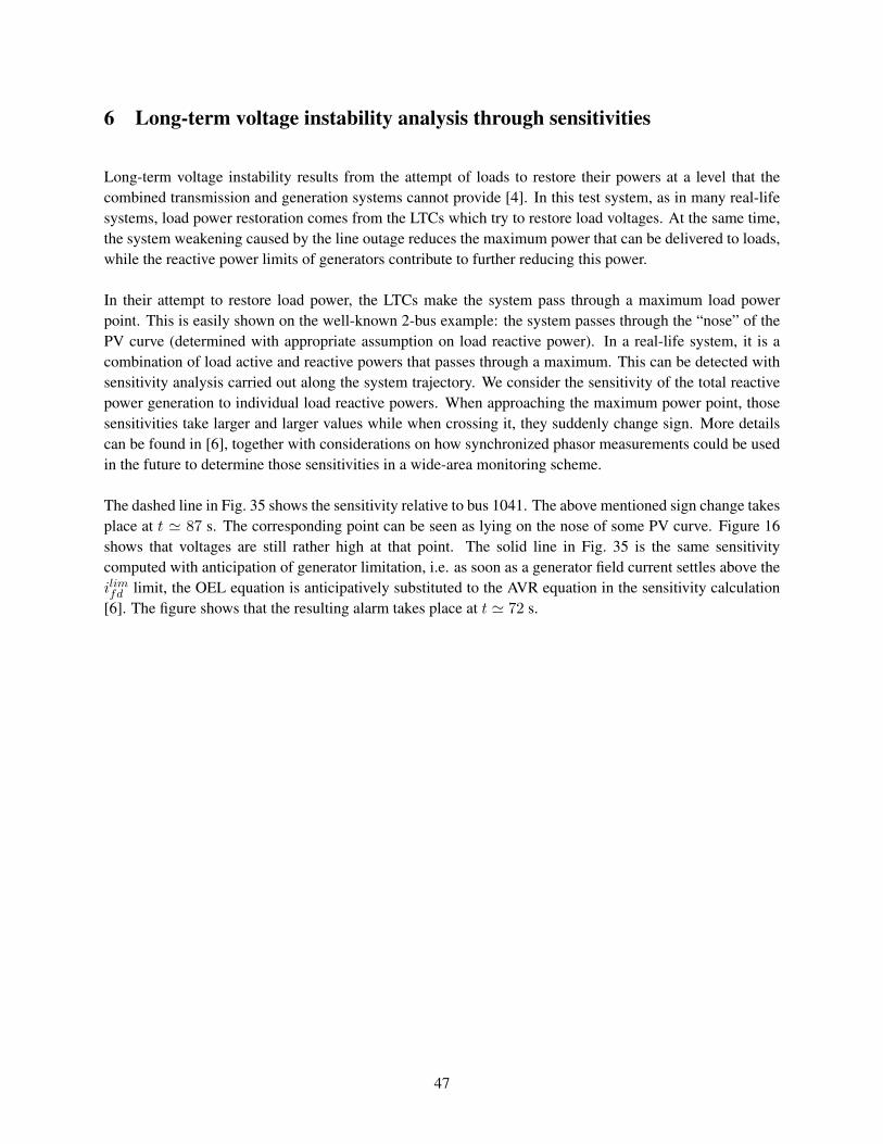
In their attempt to restore load power, the LTCs make the system pass through a maximum load powerpoint. This is easily shown on the well-known 2-bus example: the system passes through the “nose” of thePV curve (determined with appropriate assumption on load reactive power). In a real-life system, it is acombination of load active and reactive powers that passes through a maximum. This can be detected withsensitivity analysis carried out along the system trajectory. We consider the sensitivity of the total reactivepower generation to individual load reactive powers. When approaching the maximum power point, thosesensitivities take larger and larger values while when crossing it, they suddenly change sign. More detailscan be found in [6], together with considerations on how synchronized phasor measurements could be usedin the future to determine those sensitivities in a wide-area monitoring scheme.
The dashed line in Fig. 35 shows the sensitivity relative to bus 1041. The above mentioned sign change takesplace at t ≃ 87 s. The corresponding point can be seen as lying on the nose of some PV curve. Figure 16shows that voltages are still rather high at that point. The solid line in Fig. 35 is the same sensitivitycomputed with anticipation of generator limitation, i.e. as soon as a generator field current settles above theilimfd limit, the OEL equation is anticipatively substituted to the AVR equation in the sensitivity calculation[6]. The figure shows that the resulting alarm takes place at t ≃ 72 s.
47
0 20 40 60 80 100 120 140 160 180
−60
−40
−20
0
20
40
60
80
100
120
t (s)
∂ Qg/∂ dQ
l
without anticipationwith anticipation
Figure 35: ∂Qg/∂Ql at bus 1041
References
[1] M. Stubbe (Convener), Long-Term Dynamics - Phase II, Report of CIGRE Task Force 38.02.08, Jan.1995
[2] P. Kundur, Power System Stability and Control, Mc Graw Hill, EPRI Power System Engineering Series,1994
[3] C. W. Taylor, Power System Voltage Stability, EPRI Power System Engineering Series, McGraw Hill,1994
[4] T. Van Cutsem, C. Vournas, Voltage stability of electric power systems, Springer (previously KluwerAcademic Publishers), Boston (USA), 1998, ISBN 0-7923-8139-4
[5] C. Vournas, T. Van Cutsem, “Local Identification of Voltage Emergency Situations”, IEEE Trans.on Power Systems, Vol. 23, No 3, 2008, pp. 1239-248. Available at http://ieeexplore.ieee.org (DOI10.1109/TPWRS.2008.926425) and http://hdl.handle.net/2268/3194
[6] M. Glavic, T. Van Cutsem, “Wide-area Detection of Voltage Instability from Synchronized Phasor Mea-surements. Part I: Principle. Part II: Simulation Results”, IEEE Trans. on Power Systems, Vol. 24,2009, pp. 1408-1425. Available at http://ieeexplore.ieee.org (DOI 10.1109/TPWRS.2009.2023272) andhttp://hdl.handle.net/2268/7885
48

[7] B. Otomega, T. Van Cutsem, “Undervoltage load shedding using distributed controllers”, IEEE Trans.on Power Systems, Vol. 22, No 4, 2007, pp. 1898-1907. Available at http://ieeexplore.ieee.org (DOI10.1109/TPWRS.2007.907354) and http://hdl.handle.net/2268/3050
49