Deriving Signal Performance Metrics from Large-Scale

DERIVING SIGNAL PERFORMANCE METRICS FROM LARGE-SCALE 1

CONNECTED VEHICLE SYSTEM DEPLOYMENT 2

3

Joerg Christian Wolf 4

Electronics Research Lab 5

Volkswagen Group of America 6

500 Clipper Drive, Belmont, CA 94002 7

Tel: +1 650 496 7092; Email: [email protected] 8

9

Jingtao Ma 10

Traffic Technology Services, Inc. 11

17933 NW Evergreen Pkwy, Ste 240 12

Beaverton, OR 97006 13


15

Bill Cisco 16





21

Justin Neill 22





27

Brian Moen 28

City of Frisco, Texas 29

6101 Frisco Square Boulevard, Third Floor 30

Frisco, Texas 75034 31


33

Curtis Jarecki 34

City of Frisco 35

6101 Frisco Square Boulevard, Third Floor 36

Frisco, Texas 75034 37

Tel: 972-292-5457; Email: [email protected] 38

39

Word count: 5,570 words text + 7 tables/figures x 250 words (each) = 7,320 words 40

41

42

43

44

July 30, 2018 45

TRB 2019 Annual Meeting Paper revised from original submittal.

Wolf, Ma, Cisco, Neill, Moen, Jarecki 2

ABSTRACT 1

This paper documents the development of signal performance metrics (SPM) from connected 2

vehicle data, including application to existing deployment locations in the US. The metrics are 3

aggregated from anonymized vehicle traces traversing signalized intersections that are part of a 4

system deployment that is completely based on existing communication and signal control 5

infrastructure. No retrofit to controllers are necessary. The system structure consists of (1) traffic 6

signal data collection via real-time data polling, (2) signal state prediction and Signal Phase and 7

Timing (SPAT) message generation, (3) data dissemination of SPAT and Map data (MAP) 8

messages, and (4) in-vehicle applications including count-down timers, speed advice to avoid 9

stops, and emerging applications such as powertrain management or automatic engine start/stop 10

functions. Four vehicle metrics are constructed including a velocity profile, arrivals by phase state 11

(green, red), delay, and split failures. A large-scale case study in the City of Frisco, TX shows 12

potential in helping daily management of traffic signal control, and potentially improving traffic 13

flows. The connected vehicle SPMs are imported and visualized in a business intelligence tool 14

(Microsoft Power BI) to deliver a signal intelligence report comprised of a series of interactive 15

data dashboards. This interactive report provides a web-based or stand-alone interface to 16

individual signals, or corridor or citywide measures of average vehicle delay, split failures, and 17

arrival states. 18

19

20

21

22

Keywords: connected vehicle, signal performance, vehicle data, signal prediction, Power BI, big 23

data, SPAT, MAP, cellular, V2X, V2I 24

25



INTRODUCTION 1

Measuring traffic signal operations and integrating the performance metrics into business processes is now 2

accepted by an increasing number of agencies and supported by signal vendors and other industry partners 3

[1 - 3]. These signal performance metrics or SPMs allow traffic engineers to analyze the degradation or 4

improvement of signal operations over time, examine the effect resulting from any signal timing changes or 5

offset adjustments among many other management and operation needs. From these analyses and support, 6

decisions can be made with confidence to resource allocation and system planning. For example, through 7

the visualization tool of Purdue Coordination Diagram, a deficient offset setting was recognized; later offset 8

adjustments led to higher vehicle arrivals on green and thus smoother flow [4]. 9

10

At the finest granular level, two main data sources serve as input to calculate the metrics: the signal 11

controller event data, and traffic detection events. These events are recorded at 1/10 second frequency in the 12

capability enhanced controllers or by a separate data recorder [5]. From these detailed recorded events, the 13

SPMs are directly visualized (e.g. vehicle or pedestrian detection events along the time) or computed 14

combining both sources. Certain assumptions are made to assist the computation; the vehicle arrival profile 15

at the stop line takes in the green start/end times and offsets the detection on/off events by the constant 16

travel times from advance detection cross-section to the stop line [2, Chapter6]. Further metrics such as the 17

maximum queue length would also require shockwave calculation methodology to estimate the queue 18

growth and dissipation beyond advance detection [6]. 19

20

A third category of input is aggregate probe data, calculated from the traces left by the vehicle navigation 21

GPS units or travelers’ mobile devices, either triangulated from cellular connections [7], or MAC address 22

matching between sequential receiver stations [8]. The output is typically the travel times or speeds as the 23

inverse, between two known locations, or map-matched to roadway segments [3, Chapter 10]. These data 24

prove useful in congestion monitoring, and route guidance, but also for evaluating coordination quality at 25

signalized corridors [3]. Extending toward this specific purpose, researchers also developed dedicated tools 26

to leverage the power of smart phones or tablets for multi-faceted assessment. For example, TranSync [20] 27

is an iOS application that includes constructing the time-space diagram and overlaying recorded or 28

projected signal timing with detailed probe vehicle traces. The vehicle stopped times and travel times allow 29

for an intuitive and direct look at the signal phase sequence and offset setting deficiencies. 30

31

Connected Vehicle (CV) technology and applications have arisen in recent years and are enthusiastically 32

embraced by the public sector and multi-sector ITS, communications, and automotive industries. For the 33

traffic engineering community to benefit from the CV technologies, a partnership relationship is well 34

recognized as a necessary foundation in pilot studies. For example, the family of Multi-modal Intelligent 35

Traffic Signal System (MMITSS) applications see their support from government agencies of signal 36

operations, participation of emergency, freight or transit fleet operators, system upgrades by signal vendors, 37

and technology development by automotive Tier 1 suppliers. Signal controllers upgraded with roadside unit 38

(RSU) and communication capabilities allow for the needed data flowing between infrastructure and 39

vehicles equipped with onboard units (OBU) [9]. Similar partnership proved its value in pilot studies in EU 40

[10] and Canada [11]. For its nature of pilot studies, however, participating vehicle fleet is typically limited 41

both in fleet size and length of test period, with few exceptions of large scale tests spanning months [12,13]. 42

This consequently limited the use case to derive signal performance metrics for regular signal engineering 43

practices in the test area. 44

45

Recognizing the gap between CV technology development and needs for SPMs from probe data, this study 46

leverages an existing application from a recent development work [14] and large-scale applications [15], to 47

derive the SPMs from the general consumers in equipped vehicles. The purpose of this study is aiming to 48

extract SPMs from this CV application and examine its usefulness in signal operational practices. 49

50

51



This paper is organized as follows: First, the cellular Vehicle to Infrastructure (V2I) system is described, 1

including the overall system structure comprised of traffic signal data connection, signal state prediction 2

and SPAT message generation, data dissemination, and in-vehicle application. Next, the data elements are 3

described in more detail, including the MAP and SPAT messages on the server-side, and the geo-location 4

data on the vehicle-side. The resulting metrics that can be queried are then discussed. These include 5

vehicular velocity profiles, arrivals by phase state, delays, and split failures. The large-scale application of 6

this system in Frisco, Texas is then presented, including the connected vehicle SPMs which are displayed 7

via interactive data dashboards. A discussion on how the City uses these metrics in traffic planning is also 8

presented. Lastly, study limitations and future work are discussed. 9

10

SYSTEM OVERVIEW 11

This section describes the overall system architecture, sub-systems, and their roles in generating the 12

performance metrics. This system has been developed and demonstrated in different places [14], and 13

recently been deployed in mass production vehicles [15]. At the time of reporting, the system is in operation 14

supporting drivers at thousands signalized intersections. 15

16

Overall system structure 17

The following simplified chart illustrates the workflow of the eco-approach and departure system based on 18

cellular network delivery. 19

20 Figure 1. Real-time traffic light information system via cellular network. 21

Traffic Signal Data Collection 22

The traffic signal data collection sub-system (refer to 1a and 1b in Figure 1) is the interface to the traffic 23

signal control infrastructure. The real-time data polling runs every second to query the following data at a 24

minimum from either the signal controller directly (1a), or tied with Signal Management Systems (SMS) at 25

Traffic Management Centers (TMC) (1b, e.g., ATMS.Now, TranSuite, Tactics and so on). 26

- Current signal timing plan 27

- Cycle second (if running on a coordination plan) 28

- Phase call or detection call (pedestrian, bicycle, vehicle, transit) 29

- Transit Signal Priority (TSP) or preemption status 30

These data are used to feed into the SPAT data generator system. This system requires a live data connection 31

running every second from end to end traffic light via networks to the vehicle. Time delays and performance 32

is a challenge in this setup. It is important to synchronize the clocks of the system and create time stamps so 33

the receiver can determine the delay due to the network. The traffic light is not necessarily required to have 34

4G antenna

TMC

4G Cell Tower

SPAT

Data Generator

Auto OEM

Backend

1a

1b

2 3

4



a fiber optic connection, radio-based systems or wireless broadband is also feasible. 1

2

Signal State Prediction and SPAT Generation 3

SPAT data generation (refer to 2 in Figure 1) lies at the center of the overall system. Typically, SPAT data 4

conform to an industry standard such as SAE J2735 [16]. In the SPAT data, one data element that is 5

particularly important to provide in-vehicle applications is the next signal switch times, i.e., 6

MovementPhaseStatus. For actuated or adaptive signals, predicting the signal state changes becomes an 7

essential task, and various methods have been documented [17, 18]. Overall, these methods must analyze 8

both historical patterns and current traffic conditions including vehicle actuations, signal priorities, and 9

preemptions, to provide the best estimate of future signal state change times. Real-time data fusion becomes 10

crucial for traffic-actuated controls as the signal timing adjusts according to different traffic arrival patterns. 11

In this study, the primary prediction method is based on emulating the exact operations of traffic signal 12

controllers, as described in Prediction of traffic signal state changes [17] (Figure 2). 13

14

Figure 2. Emulation-based signal state change prediction workflow ([17])

15

The emulator program replicates both the signal control logic and control parameters as reflected by 16

controller firmware and timing plan data respectively. When input with the same detection, the emulator 17

program will react exactly as the field controller and generate the signal output, including signal group state 18

changes. The traffic pattern is simplified into signal phase calls (vehicle phase, public transit, pedestrian 19

push buttons or bicycle specific phases); fusing long-term calls, immediate past call history and current call 20

status, the probability of phase call activation or extension is forecast for the next few cycles (prediction 21

horizon). This forecast call spectrum is coupled to the emulator program, fast-forwarding to the end of the 22

prediction horizon. The generated signal output will then become the predicted signal state changes. This 23

method was validated in the field in multiple countries [14] and provides the most important data element in 24

the SPAT message. 25

26

27



Data dissemination 1

After SPAT data are generated, the data elements are formatted in a light-weight package and sent to the 2

backend server system of car manufacturers (refer to 3 – auto OEM backend in Figure 1). The primary 3

function of the data dissemination system is to send only the SPAT data of interested intersections to the 4

vehicles or mobile devices on the road. This includes map-matching the vehicle position to the navigation 5

network and the intersection approaches for the targeted SPAT data. 6

One critical issue in the data transmission is the compensation for all possible time lapses at each step in this 7

data chain. For example, the compensation could include the latency of data transmission from field 8

controller to SMS, collecting time from SMS to the prediction system, computing time and forwarding 9

times. All timestamps must be calibrated in the final delivery to drivers or engine management. 10

11

In-vehicle applications 12

Typical in-vehicle applications of the SPAT data are eco-approach and departure systems, which provides 13

either the simple countdown timers to display the remaining red time; Figure shows one example of such 14

red countdown timer in the dashboard. The system shown in figure 3 relies on receiving a MAP message for 15

the intersection layout. When the vehicle is matched to an approach it will show the remaining red time in 16

the dashboard using a live connection of SPAT message through the network shown in Figure 1. 17

Furthermore, the vehicle can also show a recommended speed (<= to the speed limit) to arrive at 18

intersection at the intersection on a green phase. This feature is called GLOSA (Green Light Optimized 19

Speed Advisory) [24]. Reliable reference speed limits are available through the vehicle’s camera based 20

traffic sign recognition. [23] Other implementations were documented in various studies [21]. Other 21

emerging applications such as powertrain management functions have also proven successful [19]. 22

23

Figure 3. Examples of in-vehicle human machine interface (HMI) designs that present traffic signal data to

drivers: red countdown timer (Audi Connect - Traffic Light Information)

24

Data Elements 25

For the system to return connected vehicle data, the Traffic Light Information (TLI) service must be active 26

and receive MAP and SPAT data from the backend. At the same time, once the returned vehicle trajectory 27

data is uploaded to the OEM backend, the performance metrics can then be aggregated. 28



1

Server side: MAP and SPAT messages 2

MAP message. The MAP message [16] defines the detailed intersection geometric data. As a 3

comprehensive message set, the MAP message can include multimodal information, traffic restrictions, 4

right-of-way and any other static info needed for surface traffic. The key data elements in this application 5

system is the signal phase matched to movement. At the same time, this data element is the key for phase 6

specific SPM calculations in aggregation of connected vehicle data. 7

In the system, the MAP messages are stored in the backend server, and are delivered to the onboard 8

computer only when the vehicle is approaching certain intersections; a version control mechanism is 9

designed to ensure only up-to-date MAP messages are kept onboard. 10

11

SPAT message. In this application, the key SPAT data elements include: 12

- signal group ID, 13

- timestamp of prediction, 14

- current signal status such as protected red/green, and permissive green (or flashing yellow arrow), 15

- Predicted signal switch times, 16

- Quality of prediction (confidence levels), 17

- Min/max time to switch times, 18

- Emergency vehicle preemption/public transit priority, and 19

- Status/failure mode. 20

All data elements are used as filters or certain parameters for the in-vehicle applications. For example, the 21

confidence levels serve as a filter to decide whether the service will be displayed to the drivers. 22

The SPAT message is delivered every second; when the vehicle is matched to certain signalized 23

intersections, only the SPAT for that signal is queried and delivered to the onboard computer. 24

25

Vehicle Side 26

The vehicle reports anonymized geo-locations with Network Time Protocol (NTP) synchronized 27

timestamps. This is only done when in the vicinity of an intersection and while the traffic light information 28

countdown is active in the vehicle for this intersection. The time synchronization and frequency of the data 29

points are better than with other commercially available vehicle probe data. 30

31

METRICS 32

The server constructs four (4) vehicle metrics: a velocity profile, arrival on phase state (green or red), total 33

delay, and split failures. The metrics are aggregated as sum or average per hour at the OEM backend. 34

35

Velocity metrics 36

A speed profile of the vehicle approaching the intersection is created. The vehicle may have sampled the 37

velocity at several varying points. To estimate the velocity at a given distance (e.g. 100m, 150m, 200m, 38

300m) from the stop-bar, the nearest 2 sampled geo-locations (𝑥1, 𝑥2) and their velocities (𝑣1 , 𝑣2 ) are 39

interpolated assuming linear motion and constant acceleration. 40

The constant acceleration between two geo-locations is given by 41

𝑎 =𝑣2

2−𝑣12

2(𝑥2−𝑥1) (1) 42

A sanity check is added to limit it to +/- 9.81. To avoid a division by 0 we can assume x2-x1 to be at least 43

0.01m. 44



The aim is to derive velocity in terms of distance the desired measurement points can be set by the server. 1

e.g. v(x)= v(100m) = 14.55 m/sec 2

3

𝑎 =𝑑𝑣

𝑑𝑡=

𝑑𝑣

𝑑𝑥

𝑑𝑥

𝑑𝑡 (chain rule) (2) 4

𝑎 = 𝑣𝑑𝑣

𝑑𝑥 (3) 5

𝑣 𝑑𝑣 = 𝑎 𝑑𝑥 (4) 6

∫ 𝑣 𝑑𝑣𝑣2

𝑣1= ∫ 𝑎 𝑑𝑥

𝑥2

𝑥1 (5) 7

1

2(𝑣2

2 − 𝑣12) = 𝑎(𝑥2 − 𝑥1) (6) 8

𝑣(𝑥) = √𝑣12 − 2𝑎(𝑥2 − 𝑥1) (7) 9

10

Approach velocity is a simple metric that can be measured regardless if traffic light status data is available 11

or the turn-maneuver of the car is known. Furthermore, the velocity is a critical data element for estimating 12

the free flow speed and deriving the delay. 13

14

Arrival on green/red and delay metrics 15

With traffic status data, it is possible to determine if the car is arriving when the signal status is “red” or 16

“green”. It is debatable how to define “arriving” at an intersection. It is usually defined as crossing an 17

advanced detector with an additional offset [1]. We define arriving as crossing a virtual line at 150 meters 18

before the stop-bar, without any offset of any kind. The distance is chosen since we want to capture the 19

arriving cars, but since there is a queue they might not stop all the way at the stop-bar. 20

21

An interesting metric, together with the arrival status, is the total delay. With connected vehicles it is 22

possible to measure the actual total delay. The total delay is the time lost compared to driving through the 23

junction without slowing down. To know the ideal travel time without slowing down one must assume a 24

vehicle speed. The posted speed limit may be used or alternatively a speed derived from measured speeds. 25

The posted speed limit may not be always available in a computer database. It is simpler to derive it from 26

measured speeds and reflects the real road conditions like curvature, etc. that may influence the ideal 27

vehicles’ speed. As a reference, the 85th percentile speed of the vehicles approaching on green at 150m 28

before the junction, v150g, is used. This reference (85th percentile) speed, v150g,85th, is calculated from 29

historical crossings, regardless of the requested timeframe for this report. 30

31

The reference travel time is: 32

𝑡𝑟 =150𝑚

𝑣150𝑔,85𝑡ℎ (8) 33

34

The actual travel time is: 35

𝑡𝑎 = 𝑡𝑖𝑚𝑒𝑠𝑡𝑎𝑚𝑝𝑐𝑟𝑜𝑠𝑠𝑖𝑛𝑔 − 𝑡𝑖𝑚𝑒𝑠𝑡𝑎𝑚𝑝150𝑚 (9) 36

37

The total delay is: 38

𝑡𝑑 = 𝑡𝑎 − 𝑡𝑟 (10) 39

40

The average total delay is the sum of all total delays divided by the number of crossings 41

𝑡𝑎𝑡𝑑 =∑ 𝑡𝑑𝑖

𝑛 (11) 42

for a given phase. 43

44

45



Volume Metrics 1

A simple but useful metric is the number of connected vehicles that crossed the intersection. Using the 2

geo-locations, it is possible to determine the maneuver of the vehicle (e.g. left turn, right turn). This is 3

simply done by measuring the angle of its trajectory when coming into the intersection vs. leaving the 4

intersection. A triangle larger than the intersection itself should be used so that intersection internal 5

geometry and position error are ignored. 6

7

Furthermore, a navigation map can be used to determine the size of an intersection and which parts are 8

“internal”. Once the maneuver of a vehicle through the intersection is known, it is possible to determine the 9

traffic signal it has used. Only a limited number of vehicles are participating (compared to the overall traffic 10

volume), however, at major arterials there are enough participating vehicles to get an overall impression of 11

the traffic volume when aggregated over time. 12

13

Split Failure Metrics 14

The precise number of probe vehicles that experience split failures, sometimes called cycle failure, can be 15

measured with connected vehicles. We define arriving at the intersection as being closer than 150m from 16

the limit line. From this point the traffic light state is checked until passing the limit line. Being in the red 17

state a second time before crossing is considered a split failure. 18

19

LARGE SCALE APPLICATION: FRISCO, TEXAS 20

The developed real-time traffic light information system was accepted by one automotive OEM (Audi of 21

America) as the world’s first fully integrated traffic light vehicle-to-infrastructure (V2I) application 22

implemented in production vehicles. After its service start, the general drivers of select vehicle models can 23

experience the service in their daily commute through the signalized intersections at different cities [15]. As 24

a result, the drivers begin contributing to the overall transportation system by their vehicles’ V2I 25

communication. 26

27

To examine whether the system can offer additional value to traffic management practices, the City of 28

Frisco, Texas application is used as a case study. In 2017, the Traffic Light Information service was turned 29

on for general Audi vehicle drivers through the intersections. Since then, the data are archived on the auto 30

OEM’s backend, and aggregated according to the specifications described in section 2. The study team then 31

developed the data models and specified the data aggregation intervals. This study incorporated data for the 32

six-month period from December 2017 to May 2018 at 95 signalized intersections. 33

34

The connected vehicle SPMs are imported and visualized in a business intelligence tool (Microsoft Power 35

BI) to deliver a signal intelligence report. This interactive report provides a web-based or stand-alone 36

interface to individual signals, or corridor or citywide measures. The study team developed the data model 37

and report organization by the following filters. 38

39

The filters are individualized and selectable; when no filters are applied, it will refer to the entire city or 40

region. 41

Geo-reference: the signals are referenced by individual signals, or corridors. This is made possible by the 42

signal ID and cross streets names in the MAP data. 43

Date/time grouping: For privacy concerns, the current data aggregation is by month; therefore, the date 44

range is monthly. 45

Day grouping: By usual traffic engineering analysis convention, the data are aggregated by three day 46

groups: Monday – Thursday, Friday, and Saturday-Sunday. 47

Time of days: the data are aggregated by hours. 48



Citywide overview 1

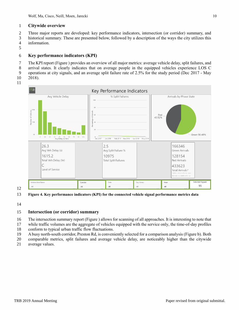
Three major reports are developed: key performance indicators, intersection (or corridor) summary, and 2

historical summary. These are presented below, followed by a description of the ways the city utilizes this 3

information. 4

5

Key performance indicators (KPI) 6

The KPI report (Figure ) provides an overview of all major metrics: average vehicle delay, split failures, and 7

arrival states. It clearly indicates that on average people in the equipped vehicles experience LOS C 8

operations at city signals, and an average split failure rate of 2.5% for the study period (Dec 2017 - May 9

2018). 10

11

12

Figure 4. Key performance indicators (KPI) for the connected vehicle signal performance metrics data 13

14

Intersection (or corridor) summary 15

The intersection summary report (Figure ) allows for scanning of all approaches. It is interesting to note that 16

while traffic volumes are the aggregate of vehicles equipped with the service only, the time-of-day profiles 17

conform to typical urban traffic flow fluctuations. 18

A busy north-south corridor, Preston Rd, is conveniently selected for a comparison analysis (Figure b). Both 19

comparable metrics, split failures and average vehicle delay, are noticeably higher than the citywide 20

average values. 21


https://app.powerbi.com/reports/8e946a5d-842c-4034-9ef8-9b666ca2615e/ReportSection9032642487b8f1bbe96e?pbi_source=PowerPoint


(a)

(b)

Figure 5. Individual intersection or corridor wide summary by approach. (a) citywide summary (b) corridor

specific summary

1

2


https://app.powerbi.com/reports/8e946a5d-842c-4034-9ef8-9b666ca2615e/ReportSection?pbi_source=PowerPoint


Historical summary 1

A historical summary report provides trendlines for arrivals, average vehicle delay and split failures (Figure 2

6). In this report view, the movement specific split failures are also separated; as expected, the split failures 3

for left turn movements happen much more frequently than other movements. 4

5

6

Figure 6. Historical summary view: SPM trendlines and movement specific aggregates 7

8

City Usage of the Data Analytics 9

The City of Frisco uses this data for multiple purposes. Evaluating the signal performance operations 10

metrics and trends over time throughout the city is a key application. This can serve to alert to the City when 11

the performance metrics have changed significantly, which is a call to action for further investigation. The 12

City also provides feedback to the public on signal operations in terms of arrivals on green %s, delays, and 13

split failures. Additionally, the data is utilized as part of evaluating the effectiveness of various intersection 14

improvements by evaluating before-and-after conditions. These include signal re-timings (including 15

addressing residents’ complaints), changes to approach geometries, and signal phasing changes, among 16

others. Examining intersection operations and planning options such as evaluating performance of 17

protected/permissive lefts compared to protected lefts is another use case. Further, the City is exploring 18

using this data as input when developing a corridor performance index for ongoing evaluations of 19

operations along key corridors. In the future, the City plans to explore how the data can help inform 20

reliability over time as well. 21

22

23

24

25

Comparison of Probe SPM vs Loop Detector SPM 26

27

We have analyized the Probe SPM data of one intersection in Frisco (TX) in May 2018 aggregated 28

Mon-Friday peak hours and compared it to the Trafficware SPM data. 29


https://app.powerbi.com/reports/8e946a5d-842c-4034-9ef8-9b666ca2615e/ReportSection9ef5aacb6f649a1d8fff?pbi_source=PowerPoint


1

Approach Delay (s/veh), Intersection #660: Preston Rd & Main St

Entire Day

AM Peak Plan 1

(7am - 9am)

PM Peak Plan 5

(4pm to 7pm)

Source SB WB NB SB WB NB SB WB NB

SPM

(Trafficware) 16.3 33.4 10.7 17.2 32.5 10.8 13.6 47.0 13.4

Vehicle Probe 55.0 53.5 30.7 80.2 40.3 36.4 30.3 148.4 48.7

Difference 38.7 20.1 20.0 63.0 7.8 25.6 16.7 101.4 35.3

2

Arrival on Red Percentage, Intersection #660: Preston Rd & Main St

Entire Day

AM Peak Plan 1

(7am - 9am)

PM Peak Plan 5

(4pm to 7pm)

Source SB WB NB SB WB NB SB WB NB

SPM

(Trafficware) 46% 71% 33% 44% 57% 29% 33% 80% 29%

Vehicle Probe 38% 70% 45% 26% 44% 50% 31% 94% 30%

Difference -8% -1% 12% -18% -13% 21% -2% 14% 1%

3 Figure 7: Approach Delay and Arrivals on Red Percentage, Trafficware SPM vs Vehicle Probe SPM. The delay 4 for the probe vehicles is calculated as the difference in travel time from the point 150m upstream of the stop 5 bar based on the probe vehicle's speed compared to the 85th-percentile speed of all probe vehicles. For the 6 SPM (Trafficware), the delay is calculated based on arrival actuations at the setback detector and adjusted for 7 travel time to the intersection stop bar. The setback detectors for this signal are located at approximately as 8 follows: 450' for SB, 450' for WB, and 365' for NB. 9 10

The delays for the probe vehicles are consistently higher than those calculated by the Trafficware SPMs. 11

Serveral factors contribute to the differences between the delays calculated by the Trafficware SPM system 12

and those calculated for the probe vehicles. One could consider potential differences in the ways the delay 13

values are determined. The probe vehicle takes into account when the vehicle actually crosses the stop bar 14

while the Trafficware SPM calculates the delay until the phase turns green and does not take into account 15

time for the vehicle in a queue waiting to get moving until reaching the stop bar. 16

Furthermore, the setback detectors, from which point the delays are measured in the Trafficware SPM 17

calculations, are located at about 450 feet (137 meters) in advance of the SB and WB stop bars, and about 18

365 feet (111 meters) in advance of the NB stop bar. For SB and WB, these are similar distances to the 150 19

meters used for the probe vehicles. For NB, the shorter distance could contribute to smaller delay 20

calculations. The probe vehicle delays are determined as the difference between the travel time from the 21

150 meter point upstream of the signal for the probe vehicle and for the 85th percentile speed. If the 85th 22

percentile speed of probe vehicles is significantly higher than the average vehicle, this could lead to the 23

probe delays being reported higher than the typical delay. Additionally, the limited sample size of the probe 24

vehicles could affect the results. We noted that the probe vehicles (Audis) do not follow the same 25

distribution for a traffic count throughout different times of the day compared to the overall traffic count. 26

Audi drivers are more likely to be found during peak hours. Finally, it is unknown whether or not the 27

Trafficware SPM delays have been compared to other field collected delays to ascertain their validity either. 28

The preceding statements are only conjectures in the absence of knowing the cause(s) for the differences 29

with certainty. 30

31

The comparison of arrivals on red as determined by the Trafficware SPMs and the probe vehicle evaluations 32

yields differences between roughly 1% - 20% depending on approach and time period. The daily 33

differences range between 1% - 12%, the a.m. peak differences range between 13% - 21%, and the p.m. 34

peak differences range between 1% - 14%. 35



STUDY LIMITATIONS AND FUTURE WORK 1

In this large-scale study, the signal performance metrics from connected vehicle data proves useful in 2

monitoring and evaluating operational performance. It particularly helps in long-term and ongoing 3

monitoring of the signal operations. The main limitation from this system is that currently only one specific 4

vehicle fleet (equipped and connected Audi vehicles) contributes to the metrics; it accounts for about 1.3% 5

of the new cars entering market nationwide and thus an even less percentage of total traffic [22]. As the 6

system may be deployed by other auto makes and models as well as more vehicles from the same fleet, the 7

sampling rate is expected to grow, reflecting the signal operations more representatively. With detector 8

loops it is possible to get close to the true number of vehicles. With this connected vehicle method, it is 9

possible to determine the split of vehicular movements (percentage that turned left, right, etc.). A 10

combination can give a traffic engineer the complete picture. The data in this paper represents only the 11

currently connected the vehicle data, it is not extrapolated to the full volume. However, the data is more 12

accurate than traditional traffic engineering methods that do not rely on connectivity. 13

This system is designed to be self-supported with its main data input (MAP and SPAT messages) and 14

vehicle probe data; it relies on no external data for more comprehensive measures. However, it is 15

anticipated that fixed-detection data such as high-resolution data logs can be combined with the connected 16

vehicle data to build more consistent and comprehensive performance metrics. It is beyond the scope of this 17

paper. 18

The system will be expanded to a fully automated SPM reporting system, without needing the study team in 19

the loop for aggregations. In particular, the auto OEM backend will build an interface for the study team to 20

query the performance metrics by the aggregation filters designed in this study. The system used for this 21

case study is expected to become available to all connected cities. 22

23

CONCLUSIONS 24

The study team developed signal performance metrics from connected vehicle data and applied the system 25

to existing deployment at various cities in US. The applicable metrics are all aggregated from the 26

anonymized vehicle traces traversing the signalized intersections. The system deployment is completely 27

based on existing communication and signal control infrastructure, with no retrofit to controllers. A 28

large-scale case study in one city showed its potential in helping daily management of traffic signal control, 29

and potentially improving traffic flows to the benefit of the contributing drivers. The system streamlines the 30

evaluation of signal performance operations metrics and trends over time throughout the city, allowing the 31

city to communicate that information to the public, as well as to identify locations where actions are 32

required to meet operational objectives, and to evaluate the effectiveness of associated improvements by 33

comparing performance before and after implementation. Future work will include combination with 34

additional data such as detectors for a more comprehensive SPM reporting. With more vehicles and 35

potentially more auto makes adding to the equipped fleet, this practice-ready system is expected to increase 36

vehicle probe sampling rate, and thus provide even more representative metrics. 37

38

AUTHOR CONTRIBUTION STATEMENT 39

The authors confirm contribution to the paper as follows: study conception and design: J. Wolf, J. Ma; data 40

collection: J. Wolf; analysis and interpretation of results: J. Wolf, J. Ma, B. Cisco, J. Neill; draft manuscript 41

preparation: J. Wolf, J. Ma, B. Cisco, J. Neill, B. Moen, Jarecki. All authors reviewed the results and 42

approved the final version of the manuscript. The contents of this paper reflect the views of the authors and 43

do not necessarily reflect the official views or policies of the sponsoring organizations. 44



REFERENCES 1

1. Day, C. M., D. M. Bullock, H. Li, S. Lavrenz, W. B. Smith, and J. R. Sturdevant. 2

“Integrating Traffic Signal Performance Measures into Agency Business Processes” 3

Purdue University, West Lafayette, Indiana, in 2015 4

http://dx.doi.org/10.5703/1288284316063. 5

2. Day, C. M., M. Taylor, J. Mackey, R. Clayton, S. K. Patel, G. Xie, H. Li, J. R. Sturdevant, 6

D. Bullock. “Implementation of automated traffic signal performance measures.” ITE 7

Journal, Vol.86, No. 8, pp 27-34, in 2016 8

3. Day., C.M., D. M. Bullock, H. Li, S.M.Remias, A. Am. Hainen, R. S. Frejie, A. L. Stevens, 9

J. R. Sturdevant, T. M. Brennan. “Performance Measures for Traffic Signal Systems: An 10

Outcome-Oriented Approach” Purdue University, West Lafayette, Indiana, doi: 11

10.5703/1288284315333, in 2014 12

4. Day, C. M., R. J. Haseman, H. Premachandra, T. M. Brennan, J. S. Wasson, J. R. 13

Sturdevant, and D. M. Bullock. “Evaluation of Arterial Signal Coordination: 14

Methodologies for Visualizing High-Resolution Event Data and Measuring Travel Time.” 15

In Transportation Research Record: Journal of the Transportation Research Board, No. 16

2192, Transportation Research Board of the National Academies, Washington, D.C., pp. 17

37–49. , 2010, doi: 10.3141/2192-04. 18

5. Liu. H. X., J. Xheng, H. Hu, J. Sun. “Research Implementation of the SMART SIGNAL 19

System on Trunk Highway (TH)” 13. Research Report, Final Report, Minnesota 20

Department of Transportation MN/RC 2013-06. St. Paul, MN. 21

6. Liu. H., W. Ma, H. Hu. “Real-time queue length estimation for congested signalized 22

intersections” Transportation Research Part C, 17(4), pp 412-427. , 2009 23

7. Ma, J., H. Li, F. Yuan, T. Bauer (2013) Deriving operational origin-destination matrices 24

from large scale mobile phone data. International Journal of Transportation Science and 25

Technology, Vol 2(3). pp 183-204. 26

8. Quayle, S., P. Koonce, D. DePencier, D. Bullock. “Arterial performance measures with 27

media access code readers: Portland Oregon, pilot study.” Transportation Research 28

Record: Journal of the Transportation Research Board, No. 2192, Transportation Research 29

Board of the National Academies, Washington, D.C., 2010, pp. 185–193, in 2010, doi: 30

10.3141/2192-04. 31

9. University of Arizona, University of California PATH Program, Savari Networks, Inc., 32

Econolite, Volvo Technology (2012). MMITSS Final ConOps: Concept of Operations, 33

online 34

http://www.cts.virginia.edu/wpcontent/uploads/2014/05/Task2.3._CONOPS_6_Final_Re35

vised.pdf accessed July 2018. 36

10. Zweck, M., M. Schuch. “Traffic Light Assistant: applying cooperative ITS in European 37

cities and vehicles”, Proceedings of 2013 International Conference on Connected Vehicles 38

and Expo (ICCVE). pp 509-513, in 2013 39

11. Kent, G., A. Thompson. “Connect Vehicle Pilot Success in Ottawa: Eco Drive I2V Proof 40

of Concept Project”, presented at ITS Canada, Niagara Falls, Ontario, Canada, June 2018. 41

12. Bezzina, D., & Sayer, J. “Safety pilot model deployment: Test conductor team report” (Report 42

No. DOT HS 812 171). Washington, DC: National Highway Traffic Safety Administration. 43

June 2015 44

13. “SimTD Facts,” Safe and Intelligent Mobility, accessed December 2014, 45

www.simtd.de/index.dhtml/enEN/backup_publications/Informationsmaterial.html 46


http://dx.doi.org/10.5703/1288284316063

http://www.simtd.de/index.dhtml/enEN/backup_publications/Informationsmaterial.html


14. Bauer, T. J. Ma, F. Offermann, “An Online Prediction System of Traffic Signal Status for 1

Assisted Driving on Urban Streets: Pilot Experiences in the US, China and Germany”, ITE 2

Journal, Vol85(2), pp 37-43, in 2015 3

15. Audi of America (2016, 2018),” Audi expands Traffic Light Information”, 4

https://www.audiusa.com/newsroom/news/press-releases/2016/12/audi-launches-vehicle-to-i5

nfrastructure-tech-in-vegas, https://media.audiusa.com/en-us/releases/241, accessed July 6

2018. 7

16. SAE International. “Surface Vehicle Standard: Dedicated Short Range Communications 8

(DSRC) Message Set Dictionary”, Warrendale, PA. 2016 9

17. Bauer, T., J. Ma, K. Hatcher, “Prediction of traffic signal state changes”, US Patent and 10

Trademark Office publication US9396657B , 2016 11

18. Weisheit T., Hoyer R., “Prediction of Switching Times of Traffic Actuated Signal Controls 12

Using Support Vector Machines” In: Fischer-Wolfarth J., Meyer G. (eds) Advanced 13

Microsystems for Automotive Applications 2014. Lecture Notes in Mobility. Springer, Cham., 14

pp 121-129 15

19. Guanetti, J., Y. Kim, F. Borreli, “Control of connected and automated vehicles: state of the art 16

and future challenges”, preprint submitted to Annual Reviews in Control, 17

https://arxiv.org/pdf/1804.03757 accessed July 2018. 18

20. Styer, M. V., D. Wei, “TranSync Mobile Tool: Pilot Project in Auburn and San Francisco Bay 19

Area (Caltrans Districts 3 and 4)”, presented at Western States Rural Transportation 20

Technology Implementers Forum, Yreka, California, June 2015. 21

21. USDOT (2015). “GlidePath Prototype Application: Automated Eco-Friendly Cruise Control 22

using Wireless V2I Communications at Signalized Intersections”, 23

https://www.its.dot.gov/research_archives/aeris/pdf/GlidePathWebinar.pdf accessed July 24

2018. 25

22. Matthews, Jack, “U.S. Auto Sales Brand Rankings – December 2017 YTD”, 26

http://www.goodcarbadcar.net/2018/01/u-s-auto-sales-brand-rankings-december-2017-ytd/ 27

accessed July 2018. 28

23. Audi Media-Center, “Driver assistance systems” 29

https://www.audi-mediacenter.com/en/technology-lexicon-7180/driver-assistance-systems-7130

84 31

24. Robert Bodenheimer, David Eckhoff† and Reinhard German, "GLOSA for Adaptive Traffic 32

Lights: Methods and Evaluation", (IEEE) 7th International Workshop on Reliable Networks 33

Design and Modeling (RNDM), Munich 5 Oct, 2015, ISBN 978-1-4673-8051-5 34

35

36

37

38


https://www.audiusa.com/newsroom/news/press-releases/2016/12/audi-launches-vehicle-to-infrastructure-tech-in-vegas

https://www.audiusa.com/newsroom/news/press-releases/2016/12/audi-launches-vehicle-to-infrastructure-tech-in-vegas

https://media.audiusa.com/en-us/releases/241

https://arxiv.org/pdf/1804.03757%20accessed%20July%202018

https://www.its.dot.gov/research_archives/aeris/pdf/GlidePathWebinar.pdf

http://www.goodcarbadcar.net/2018/01/u-s-auto-sales-brand-rankings-december-2017-ytd/



Documents

Deriving Signal Performance Metrics from Large-Scale