Deriving Neural Architectures from Sequence and Graph Kernels

Tao Lei* 1 Wengong Jin* 1 Regina Barzilay 1 Tommi Jaakkola 1

AbstractThe design of neural architectures for structuredobjects is typically guided by experimental in-sights rather than a formal process. In this work,we appeal to kernels over combinatorial struc-tures, such as sequences and graphs, to deriveappropriate neural operations. We introduce aclass of deep recurrent neural operations and for-mally characterize their associated kernel spaces.Our recurrent modules compare the input to vir-tual reference objects (cf. filters in CNN) via thekernels. Similar to traditional neural operations,these reference objects are parameterized and di-rectly optimized in end-to-end training. We em-pirically evaluate the proposed class of neural ar-chitectures on standard applications such as lan-guage modeling and molecular graph regression,achieving state-of-the-art results across these ap-plications.

1. IntroductionMany recent studies focus on designing novel neural ar-chitectures for structured data such as sequences or anno-tated graphs. For instance, LSTM (Hochreiter & Schmid-huber, 1997), GRU (Chung et al., 2014) and other complexrecurrent units (Zoph & Le, 2016) can be easily adaptedto embed structured objects such as sentences (Tai et al.,2015) or molecules (Li et al., 2015; Dai et al., 2016) intovector spaces suitable for later processing by standard pre-dictive methods. The embedding algorithms are typicallyintegrated into an end-to-end trainable architecture so as totailor the learnable embeddings directly to the task at hand.

The embedding process itself is characterized by a se-quence operations summarized in a structure known asthe computational graph. Each node in the computational

*Equal contribution 1MIT Computer Science & Ar-tificial Intelligence Laboratory. Correspondence to:Tao Lei <taolei@csail.mit.edu>, Wengong Jin <wen-gong@csail.mit.edu>.

Proceedings of the 34 th International Conference on MachineLearning, Sydney, Australia, PMLR 70, 2017. Copyright 2017by the author(s).

graph identifies the unit/mapping applied while the arcsspecify the relative arrangement/order of operations. Theprocess of designing such computational graphs or asso-ciated operations for classes of objects is often guided byinsights and expertise rather than a formal process.

Recent work has substantially narrowed the gap betweendesirable computational operations associated with objectsand how their representations are acquired. For example,value iteration calculations can be folded into convolutionalarchitectures so as to optimize the representations to fa-cilitate planning (Tamar et al., 2016). Similarly, inferencecalculations in graphical models about latent states of vari-ables such as atom characteristics can be directly associatedwith embedding operations (Dai et al., 2016).

We appeal to kernels over combinatorial structures to de-fine the appropriate computational operations. Kernels giverise to well-defined function spaces and possess rules ofcomposition that guide how they can be built from simplerones. The comparison of objects inherent in kernels is of-ten broken down to elementary relations such as countingof common sub-structures as in

K(χ, χ′) =∑s∈S

1[s ∈ χ]1[s ∈ χ′] (1)

where S is the set of possible substructures. For exam-ple, in a string kernel (Lodhi et al., 2002), S may referto all possible subsequences while a graph kernel (Vish-wanathan et al., 2010) would deal with possible pathsin the graph. Several studies have highlighted the rela-tion between feed-forward neural architectures and ker-nels (Hazan & Jaakkola, 2015; Zhang et al., 2016) but weare unaware of any prior work pertaining to kernels associ-ated with neural architectures for structured objects.

In this paper, we introduce a class of deep recurrent neuralembedding operations and formally characterize their asso-ciated kernel spaces. The resulting kernels are parameter-ized in the sense that the neural operations relate objects ofinterest to virtual reference objects through kernels. Thesereference objects are parameterized and readily optimizedfor end-to-end performance.

To summarize, the proposed neural architectures, or KernelNeural Networks 1 , enjoy the following advantages:

1Code available at https://github.com/taolei87/icml17 knn

arX

iv:1

705.

0903

7v3

[cs

.NE

] 3

0 O

ct 2

017

Deriving Neural Architectures from Sequence and Graph Kernels

• The architecture design is grounded in kernel compu-tations.

• Our neural models remain end-to-end trainable to thetask at hand.

• Resulting architectures demonstrate state-of-the-artperformance against strong baselines.

In the following sections, we will introduce these neuralcomponents derived from string and graph kernels, as wellas their deep versions. Due to space limitations, we deferproofs to supplementary material.

2. From String Kernels to Sequence NNsNotations We define a sequence (or a string) of tokens(e.g. a sentence) as x1:L = {xi}Li=1 where xi ∈ Rd repre-sents its ith element and |x| = L denotes the length. When-ever it is clear from the context, we will omit the subscriptand directly use x (and y) to denote a sequence. For a pairof vectors (or matrices) u,v, we denote 〈u,v〉 =

∑k ukvk

as their inner product. For a kernel function Ki(·, ·) withsubscript i, we use φi(·) to denote its underlying mapping,i.e. Ki(x,y) = 〈φi(x), φi(y)〉 = φi(x)

>φi(y).

String Kernel String kernel measures the similarity be-tween two sequences by counting shared subsequences(see Lodhi et al. (2002)). For example, let x and y be twostrings, a bi-gram string kernel K2(x,y) counts the num-ber of bi-grams (xi,xj) and (yk,yl) such that (xi,xj) =(yk,yl)

2,

K2(x,y) =∑

1≤i<j≤|x|1≤k<l≤|y|

λx,i,j λy,k,l δ(xi,yk) · δ(xj ,yl)

(2)where λx,i,j , λy,k,l ∈ [0, 1) are context-dependent weightsand δ(x, y) is an indicator that returns 1 only when x = y.The weight factors can be realized in various ways. Forinstance, in temporal predictions such as language model-ing, substrings (i.e. patterns) which appear later may havehigher impact for prediction. Thus a realization λx,i,j =λ|x|−i−1 and λy,k,l = λ|y|−k−1 (penalizing substrings farfrom the end) can be used to determine weights given aconstant decay factor λ ∈ (0, 1).

In our case, each token in the sequence is a vector (such asone-hot encoding of a word or a feature vector). We shallreplace the exact match δ(u,v) by the inner product 〈u,v〉.To this end, the kernel function (2) can be rewritten as,∑1≤i<j≤|x|

∑1≤k<l≤|y|

λx,i,j λy,k,l 〈xi,yk〉 · 〈xj ,yl〉

2We define n-gram as a subsequence of original string (notnecessarily consecutive).

�

�

�

�

�

�

�

�

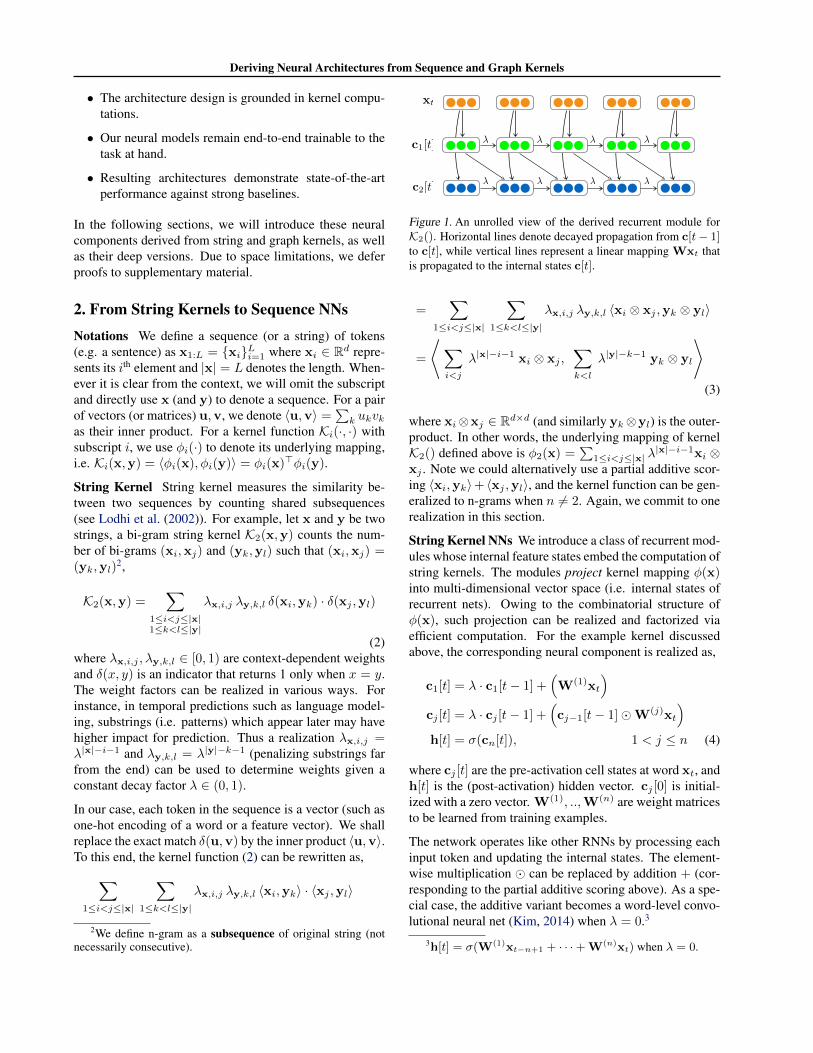
Figure 1. An unrolled view of the derived recurrent module forK2(). Horizontal lines denote decayed propagation from c[t− 1]to c[t], while vertical lines represent a linear mapping Wxt thatis propagated to the internal states c[t].

=∑

1≤i<j≤|x|

∑1≤k<l≤|y|

λx,i,j λy,k,l 〈xi ⊗ xj ,yk ⊗ yl〉

=

⟨∑i<j

λ|x|−i−1 xi ⊗ xj ,∑k<l

λ|y|−k−1 yk ⊗ yl

⟩(3)

where xi⊗xj ∈ Rd×d (and similarly yk⊗yl) is the outer-product. In other words, the underlying mapping of kernelK2() defined above is φ2(x) =

∑1≤i<j≤|x| λ

|x|−i−1xi ⊗xj . Note we could alternatively use a partial additive scor-ing 〈xi,yk〉+ 〈xj ,yl〉, and the kernel function can be gen-eralized to n-grams when n 6= 2. Again, we commit to onerealization in this section.

String Kernel NNs We introduce a class of recurrent mod-ules whose internal feature states embed the computation ofstring kernels. The modules project kernel mapping φ(x)into multi-dimensional vector space (i.e. internal states ofrecurrent nets). Owing to the combinatorial structure ofφ(x), such projection can be realized and factorized viaefficient computation. For the example kernel discussedabove, the corresponding neural component is realized as,

c1[t] = λ · c1[t− 1] +(W(1)xt

)cj [t] = λ · cj [t− 1] +

(cj−1[t− 1]�W(j)xt

)h[t] = σ(cn[t]), 1 < j ≤ n (4)

where cj [t] are the pre-activation cell states at word xt, andh[t] is the (post-activation) hidden vector. cj [0] is initial-ized with a zero vector. W(1), ..,W(n) are weight matricesto be learned from training examples.

The network operates like other RNNs by processing eachinput token and updating the internal states. The element-wise multiplication � can be replaced by addition + (cor-responding to the partial additive scoring above). As a spe-cial case, the additive variant becomes a word-level convo-lutional neural net (Kim, 2014) when λ = 0.3

3h[t] = σ(W(1)xt−n+1 + · · ·+W(n)xt) when λ = 0.

Deriving Neural Architectures from Sequence and Graph Kernels

2.1. Single Layer as Kernel Computation

Now we state how the proposed class embeds string kernelcomputation. For j ∈ {1, .., n}, let cj [t][i] be the i-th entryof state vector cj [t], w

(j)i represents the i-th row of ma-

trix W(j). Define wi,j = {w(1)i ,w

(2)i , ...,w

(j)i } as a “ref-

erence sequence” constructed by taking the i-th row fromeach matrix W(1), ..,W(j).

Theorem 1. Let x1:t be the prefix of x consisting of firstt tokens, and Kj be the string kernel of j-gram shown inEq.(3). Then cj [t][i] evaluates kernel function,

cj [t][i] = Kj (x1:t,wi,j) = 〈φj(x1:t), φj(wi,j)〉

for any j ∈ {1, .., n}, t ∈ {1, .., |x|}.

In other words, the network embeds sequence similaritycomputation by assessing the similarity between the inputsequence x1:t and the reference sequence wi,j . This in-terpretation is similar to that of CNNs, where each filteris a “reference pattern” to search in the input. String ker-nel NN further takes non-consecutive n-gram patterns intoconsideration (seen from the summation over all n-gramsin Eq.(3)).

Applying Non-linear Activation In practice, a non-linearactivation function such as polynomial or sigmoid-like ac-tivation is added to the internal states to produce the fi-nal output state h[t]. It turns out that many activationsare also functions in the reproducing kernel Hilbert space(RKHS) of certain kernel functions (see Shalev-Shwartzet al. (2011); Zhang et al. (2016)). When this is true, theunderlying kernel of h[t] is the composition of string ker-nel and the kernel containing the activation. We give theformal statements below.

Lemma 1. Let x and w be multi-dimensional vectors withfinite norm. Consider the function f(x) := σ(w>x) withnon-linear activation σ(·). For functions such as polyno-mials and sigmoid function, there exists kernel functionsKσ(·, ·) and the underlying mapping φσ(·) such that f(x)is in the reproducing kernel Hilbert space of Kσ(·, ·), i.e.,

f(x) = σ(w>x) = 〈φσ(x), ψ(w)〉

for some mapping ψ(w) constructed from w. In particular,Kσ(x,y) can be the inverse-polynomial kernel 1

2−〈x,y〉 forthe above activations.

Proposition 1. For one layer string kernel NN with non-linear activation σ(·) discussed in Lemma 1, h[t][i] as afunction of input x belongs to the RKHS introduced by thecomposition of Kσ(·, ·) and string kernel Kn(·, ·). Here akernel composition Kσ,n(x,y) is defined with the under-lying mapping x 7→ φσ(φn(x)), and hence Kσ,n(x,y) =φσ(φn(x))>φσ(φn(y)).

Proposition 1 is the corollary of Lemma 1 and Theo-rem 1, since h[t][i] = σ(cn[t][i]) = σ(Kn(x1:t,wi,j)) =〈φσ(φn(x1:t)), wi,j〉 and φσ(φn(·)) is the mapping for thecomposed kernel. The same proof applies when h[t] is alinear combination of all ci[t] since kernel functions areclosed under addition.

2.2. Deep Networks as Deep Kernel Construction

We now address the case when multiple layers of the samemodule are stacked to construct deeper networks. That is,the output states h(l)[t] of the l-th layer are fed to the (l+1)-th layer as the input sequence. We show that layer stackingcorresponds to recursive kernel construction (i.e. (l + 1)-th kernel is defined on top of l-th kernel), which has beenproven for feed-forward networks (Zhang et al., 2016).

We first generalize the sequence kernel definition to enablerecursive construction. Notice that the definition in Eq.(3)uses the linear kernel (inner product) 〈xi,yk〉 as a “subrou-tine” to measure the similarity between substructures (e.g.tokens) within the sequences. We can therefore replace itwith other similarity measures introduced by other “basekernels”. In particular, let K(1)(·, ·) be the string kernel(associated with a single layer). The generalized sequencekernel K(l+1)(x,y) can be recursively defined as,∑i<jk<l

λx,i,j λy,k,l K(l)σ (x1:i,y1:k) K(l)

σ (x1:j ,y1:l) =

⟨∑i<j

φ(l)σ (x1:i)⊗ φ(l)σ (x1:j),∑k<l

φ(l)σ (y1:k)⊗ φ(l)σ (y1:l)

⟩

where φ(l)(·) denotes the pre-activation mapping of the l-th kernel, φ(l)σ (·) = φσ(φ

(l)(·)) denotes the underlying(post-activation) mapping for non-linear activation σ(·),and K(l)

σ (·, ·) is the l-th post-activation kernel. Based onthis definition, a deeper model can also be interpreted as akernel computation.

Theorem 2. Consider a deep string kernel NN with Llayers and activation function σ(·). Let the final outputstate h(L)[t] = σ(c

(L)n [t]) (or any linear combination of

{c(l)i [t]}, i = 1, .., n). For l = 1, · · · , L,

(i) c(l)n [t][i] as a function of input x belongs to the RKHS

of kernel K(l)(·, ·);

(ii) h(l)[t][i] belongs to the RKHS of kernel K(l)σ (·, ·).

3. From Graph Kernels to Graph NNsIn the previous section, we encode sequence kernel com-putation into neural modules and demonstrate possible ex-tensions using different base kernels. The same ideas apply

Deriving Neural Architectures from Sequence and Graph Kernels

to other types of kernels and data. Specifically, we deriveneural components for graphs in this section.

Notations A graph is defined as G = (V,E), with eachvertex v ∈ V associated with feature vector fv . The neigh-bor of node v is denoted as N(v). Following previousnotations, for any kernel function K∗(·, ·) with underly-ing mapping φ∗(·), we use K∗,σ(·, ·) to denote the post-activation kernel induced from the composed underlyingmapping φ∗,σ = φσ(φ∗(·)).

3.1. Random Walk Kernel NNs

We start from random walk graph kernels (Gartner et al.,2003), which count common walks in two graphs. For-mally, let Pn(G) be the set of walks x = x1 · · ·xn, where∀i : (xi, xi+1) ∈ E.4 Given two graphs G and G′, an n-thorder random walk graph kernel is defined as:

KnW (G,G′) = λn−1∑

x∈Pn(G)

∑y∈Pn(G′)

n∏i=1

〈fxi , fyi〉 (5)

where fxi ∈ Rd is the feature vector of node xi in the walk.

Now we show how to realize the above graph kernel witha neural module. Given a graph G, the proposed neuralmodule is:

c1[v] = W(1)fv

cj [v] = λ∑

u∈N(v)

cj−1[u]�W(j)fv (6)

hG = σ(∑v

cn[v]) 1 < j ≤ n

where again c∗[v] is the cell state vector of node v, and hGis the representation of graph G aggregated from node vec-tors. hG could then be used for classification or regression.

Now we show the proposed model embeds the randomwalk kernel. To show this, construct Ln,k as a “refer-ence walk” consisting of the row vectors {w(1)

k , · · · ,w(n)k }

from the parameter matrices. Here Ln,k = (LV , LE),where LV = {v0, v1, · · · , vn}, LE = {(vi, vi+1)} and vi’sfeature vector is w(i)

k . We have the following theorem:

Theorem 3. For any n ≥ 1, the state value cn[v][k] (thek-th coordinate of cn[v]) satisfies:∑

v

cn[v][k] = KnW (G,Ln,k)

thus∑v cn[v] lies in the RKHS of kernel KnW . As a corol-

lary, hG lies in the RKHS of kernel KnW,σ().

4A single node could appear multiple times in a walk.

3.2. Unified View of Graph Kernels

The derivation of the above neural module could be ex-tended to other classes of graph kernels, such as subtreekernels (cf. (Ramon & Gartner, 2003; Vishwanathan et al.,2010)). Generally speaking, most of these kernel functionsfactorize graphs into local sub-structures, i.e.

K(G,G′) =∑v

∑v′

Kloc(v, v′) (7)

where Kloc(v, v′) measures the similarity between localsub-structures centered at node v and v′.

For example, the random walk kernel KnW can be equiva-

lently defined with Knloc(v, v′) = 〈fv, fv′〉 if n = 1

〈fv, fv′〉 · λ∑

u∈N(v)

∑u′∈N(v′)

Kn−1loc (u, u′) if n > 1

Other kernels like subtree kernels could be recursively de-fined similarly. Therefore, we adopt this unified view ofgraph kernels for the rest of this paper.

In addition, this definition of random walk kernel could befurther generalized and enhanced by aggregating neighborfeatures non-linearly:

Knloc(v, v′) = 〈fv, fv′〉 ◦ λ∑

u∈N(v)

∑u′∈N(v′)

Kn−1loc,σ(u, u′)

where ◦ could be either multiplication or addition. σ(·)denotes a non-linear activation and Kn−1loc,σ(·, ·) denotes thepost-activation kernel when σ(·) is involved. The general-ized kernel could be realized by modifying Eq.(6) into:

cj [v] = W(j)fv ◦ λ∑

u∈N(v)

σ(cj−1[u]) (8)

where ◦ could be either + or � operation.

3.3. Deep Graph Kernels and NNs

Following Section 2, we could stack multiple graph kernelNNs to form a deep network. That is:

c(l)1 [v] = W(l,1)h(l−1)[v]

c(l)j [v] = W(l,j)h(l−1)[v] ◦ λ

∑u∈N(v)

σ(c(l)j−1[u]

)h(l)[v] = σ(U(l)c(l)n [v]) 1 ≤ l ≤ L, 1 < j ≤ n

The local kernel function is recursively defined intwo dimensions: depth (term h(l)) and width (termcj). Let the pre-activation kernel in the l-th layer beK(l)loc(v, v

′) = K(l,n)loc (v, v′), and the post-activation ker-

nel be K(l)loc,σ(v, v

′) = K(l,n)loc,σ(v, v

′). We recursively define

Deriving Neural Architectures from Sequence and Graph Kernels

K(l,j)loc (v, v′) = K

(l−1)loc,σ (v, v

′) if j = 1

K(l−1)loc,σ (v, v

′) ◦ λ∑

u∈N(v)

∑u′∈N(v′)

K(l,j−1)loc,σ (u, u′) if j > 1

for j = 1, · · · , n. Finally, the graph kernel isK(L,n)(G,G′) =

∑v,v′ K

(L,n)loc (v, v′). Similar to Theo-

rem 2, we haveTheorem 4. Consider a deep graph kernel NN with L lay-ers and activation function σ(·). Let the final output statehG =

∑v h

(L)[v]. For l = 1, · · · , L; j = 1, · · · , n:

(i) c(l)j [v][i] as a function of input v and graph G belongs

to the RKHS of kernel K(l,j)loc (·, ·);

(ii) h(l)[v][i] belongs to the RKHS of kernel K(l,n)loc,σ(·, ·).

(iii) hG[i] belongs to the RKHS of kernel K(L,n)(·, ·).

3.4. Connection to Weisfeiler-Lehman Kernel

We derived the above deep kernel NN for the purpose ofgenerality. This model could be simplified by setting n =2, without losing representational power (as non-linearityis already involved in depth dimension). In this case, werewrite the network by reparametrization:

h(l)v = σ

U(l)1 h(l−1)

v ◦U(l)2

∑u∈N(v)

σ(V(l)h(l−1)

u

)(9)

In this section, we further show that this model could be en-hanced by sharing weight matrices U and V across layers.This parameter tying mechanism allows our model to em-bed Weisfeiler-Lehman kernel (Shervashidze et al., 2011).For clarity, we briefly review basic concepts of Weisfeiler-Lehman kernel below.

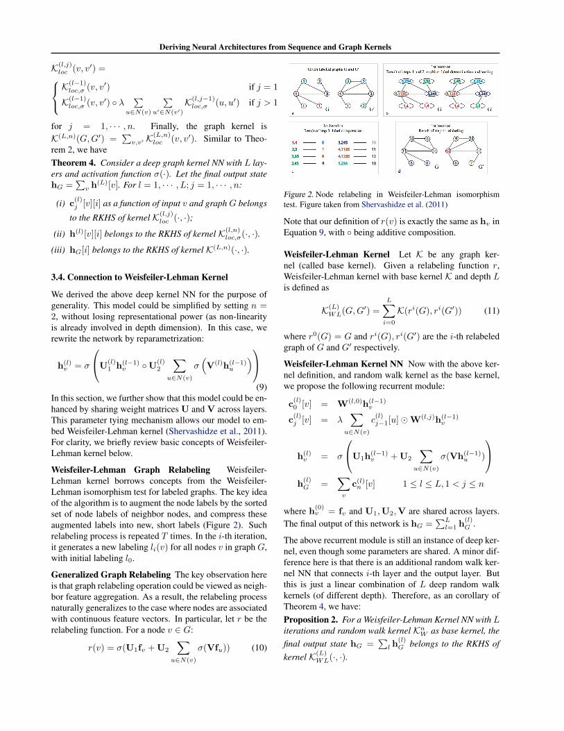
Weisfeiler-Lehman Graph Relabeling Weisfeiler-Lehman kernel borrows concepts from the Weisfeiler-Lehman isomorphism test for labeled graphs. The key ideaof the algorithm is to augment the node labels by the sortedset of node labels of neighbor nodes, and compress theseaugmented labels into new, short labels (Figure 2). Suchrelabeling process is repeated T times. In the i-th iteration,it generates a new labeling li(v) for all nodes v in graph G,with initial labeling l0.

Generalized Graph Relabeling The key observation hereis that graph relabeling operation could be viewed as neigh-bor feature aggregation. As a result, the relabeling processnaturally generalizes to the case where nodes are associatedwith continuous feature vectors. In particular, let r be therelabeling function. For a node v ∈ G:

r(v) = σ(U1fv +U2

∑u∈N(v)

σ(Vfu)) (10)

Figure 2. Node relabeling in Weisfeiler-Lehman isomorphismtest. Figure taken from Shervashidze et al. (2011)

Note that our definition of r(v) is exactly the same as hv inEquation 9, with ◦ being additive composition.

Weisfeiler-Lehman Kernel Let K be any graph ker-nel (called base kernel). Given a relabeling function r,Weisfeiler-Lehman kernel with base kernel K and depth Lis defined as

K(L)WL(G,G

′) =

L∑i=0

K(ri(G), ri(G′)) (11)

where r0(G) = G and ri(G), ri(G′) are the i-th relabeledgraph of G and G′ respectively.

Weisfeiler-Lehman Kernel NN Now with the above ker-nel definition, and random walk kernel as the base kernel,we propose the following recurrent module:

c(l)0 [v] = W(l,0)h(l−1)

v

c(l)j [v] = λ

∑u∈N(v)

c(l)j−1[u]�W(l,j)h(l−1)

v

h(l)v = σ

U1h(l−1)v +U2

∑u∈N(v)

σ(Vh(l−1)u )

h(l)G =

∑v

c(l)n [v] 1 ≤ l ≤ L, 1 < j ≤ n

where h(0)v = fv and U1,U2,V are shared across layers.

The final output of this network is hG =∑Ll=1 h

(l)G .

The above recurrent module is still an instance of deep ker-nel, even though some parameters are shared. A minor dif-ference here is that there is an additional random walk ker-nel NN that connects i-th layer and the output layer. Butthis is just a linear combination of L deep random walkkernels (of different depth). Therefore, as an corollary ofTheorem 4, we have:Proposition 2. For a Weisfeiler-Lehman Kernel NN with Literations and random walk kernel KnW as base kernel, thefinal output state hG =

∑l h

(l)G belongs to the RKHS of

kernel K(L)WL(·, ·).

Deriving Neural Architectures from Sequence and Graph Kernels

4. Adaptive Decay with Neural GatesThe sequence and graph kernel (and their neural compo-nents) discussed so far use a constant decay value λ re-gardless of the current input. However, this is often not thecase since the importance of the input can vary across thecontext or the applications. One extension is to make use ofneural gates that adaptively control the decay factor. Herewe give two illustrative examples:

Gated String Kernel NN By replacing constant decay λwith a sigmoid gate, we modify our single-layer sequencemodule as:

λt = σ(U[xt,ht−1] + b)

c1[t] = λt � c1[t− 1] +(W(1)xt

)cj [t] = λt � cj [t− 1] +

(cj−1[t− 1]�W(j)xt

)h[t] = σ(cn[t]) 1 < j ≤ n

As compared with the original string kernel, now the decayfactor λx,i,j is no longer λ|x|−i−1, but rather an adaptivevalue based on current context.

Gated Random Walk Kernel NN Similarly, we could in-troduce gates so that different walks have different weights:

λu,v = σ(U[fu, fv] + b)

c0[v] = W(0)fv

cj [v] =∑

u∈N(v)

λu,v � cj−1[u]�W(j)fv

hG = σ(∑v

cn[v]) 1 < j ≤ n

The underlying kernel of the above gated network becomes

KnW (G,G′) =∑

x∈Pn(G)

∑y∈Pn(G′)

n∏i=1

λxi,yi〈fxi

, fyi〉

where each path is weighted by different decay weights,determined by network itself.

5. Related WorkSequence Networks Considerable effort has gone into de-signing effective networks for sequence processing. Thisincludes recurrent modules with the ability to carry per-sistent memories such as LSTM (Hochreiter & Schmid-huber, 1997) and GRU (Chung et al., 2014), as well asnon-consecutive convolutional modules (RCNNs, Lei et al.(2015)), and others. More recently, Zoph & Le (2016) ex-emplified a reinforcement learning-based search algorithmto further optimize the design of such recurrent architec-tures. Our proposed neural networks offer similar state

evolution and feature aggregation functionalities but de-rive the motivation for the operations involved from well-established kernel computations over sequences.

Recursive neural networks are alternative architectures tomodel hierarchical structures such as syntax trees and logicforms. For instance, Socher et al. (2013) employs recur-sive networks for sentence classification, where each nodein the dependency tree of the sentence is transformed intoa vector representation. Tai et al. (2015) further proposedtree-LSTM, which incorporates LSTM-style architecturesas the transformation unit. Dyer et al. (2015; 2016) re-cently introduced a recursive neural model for transition-based language modeling and parsing. While not specifi-cally discussed in the paper, our ideas do extend to similarneural components for hierarchical objects (e.g. trees).

Graph Networks Most of the current graph neural archi-tectures perform either convolutional or recurrent opera-tions on graphs. Duvenaud et al. (2015) developed NeuralFingerprint for chemical compounds, where each convo-lution operation is a sum of neighbor node features, fol-lowed by a linear transformation. Our model differs fromtheirs in that our generalized kernels and networks can ag-gregate neighboring features in a non-linear way. Other ap-proaches, e.g., Bruna et al. (2013) and Henaff et al. (2015),rely on graph Laplacian or Fourier transform.

For recurrent architectures, Li et al. (2015) proposed gatedgraph neural networks, where neighbor features are ag-gregated by GRU function. Dai et al. (2016) considers adifferent architecture where a graph is viewed as a latentvariable graphical model. Their recurrent model is derivedfrom Belief Propagation-like algorithms. Our approach ismost closely related to Dai et al. (2016), in terms of neigh-bor feature aggregation and resulting recurrent architec-ture. Nonetheless, the focus of this paper is on providinga framework for how such recurrent networks could be de-rived from deep graph kernels.

Kernels and Neural Nets Our work follows recent workdemonstrating the connection between neural networks andkernels (Cho & Saul, 2009; Hazan & Jaakkola, 2015).For example, Zhang et al. (2016) showed that standardfeedforward neural nets belong to a larger space of recur-sively constructed kernels (given certain activation func-tions). Similar results have been made for convolutionalneural nets (Anselmi et al., 2015), and general computa-tional graphs (Daniely et al., 2016). We extend prior workto kernels and neural architectures over structured inputs,in particular, sequences and graphs. Another difference ishow we train the model. While some prior work appealsto convex optimization through improper learning (Zhanget al., 2016; Heinemann et al., 2016) (since kernel space islarger), we use the proposed networks as building blocks intypical non-convex but flexible neural network training.

Deriving Neural Architectures from Sequence and Graph Kernels

6. ExperimentsThe left-over question is whether the proposed class of op-erations, despite its formal characteristics, leads to moreeffective architecture exploration and hence improved per-formance. In this section, we apply the proposed sequenceand graph modules to various tasks and empirically evalu-ate their performance against other neural network models.These tasks include language modeling, sentiment classifi-cation and molecule regression.

6.1. Language Modeling on PTB

Dataset and Setup We use the Penn Tree Bank (PTB) cor-pus as the benchmark. The dataset contains about 1 milliontokens in total. We use the standard train/development/testsplit of this dataset with vocabulary of size 10,000.

Model Configuration Following standard practice, we useSGD with an initial learning rate of 1.0 and decrease thelearning rate by a constant factor after a certain epoch. Weback-propagate the gradient with an unroll size of 35 anduse dropout (Hinton et al., 2012) as the regularization. Un-less otherwise specified, we train 3-layer networks withn = 1 and normalized adaptive decay.5 Following (Zillyet al., 2016), we add highway connections (Srivastava et al.,2015) within each layer:

c(l)[t] = λt � c(l)[t− 1] + (1− λt)� (W(l)h(l−1)[t])

h(l)[t] = ft � c(l)[t] + (1− ft)� h(l−1)[t]

where h(0)[t] = xt, λt is the gated decay factor and ft isthe transformation gate of highway connections.6

Results Table 1 compares our model with various state-of-the-art models. Our small model with 5 million parametersachieves a test perplexity of 73.6, already outperformingmany results achieved using much larger network. By in-creasing the network size to 20 million, we obtain a testperplexity of 69.2, with standard dropout. Adding varia-tional dropout (Gal & Ghahramani, 2016) within the re-current cells further improves the perplexity to 65.5. Fi-nally, the model achieves 63.8 perplexity when the recur-rence depth is increased to 4, being state-of-the-art and onpar with the results reported in (Zilly et al., 2016; Zoph &Le, 2016). Note that Zilly et al. (2016) uses 10 neural lay-ers and Zoph & Le (2016) adopts a complex recurrent cellfound by reinforcement learning based search. Our net-work is architecturally much simpler.

Figure 3 analyzes several variants of our model. Word-level CNNs are degraded cases (λ = 0) that ignore non-

5See the supplementary sections for a discussion of networkvariants.

6We found non-linear activation is no longer necessary whenthe highway connection is added.

Table 1: Comparison with state-of-the-art results on PTB.|θ| denotes the number of parameters. Following recentwork (Press & Wolf, 2016), we share the input and out-put word embedding matrix. We report the test perplexity(PPL) of each model. Lower number is better.

Model |θ| PPLLSTM (large) (Zaremba et al., 2014) 66m 78.4Character CNN (Kim et al., 2015) 19m 78.9Variational LSTM (Gal & Ghahramani) 20m 78.6Variational LSTM (Gal & Ghahramani) 66m 73.4Pointer Sentinel-LSTM (Merity et al.) 21m 70.9Variational RHN (Zilly et al., 2016) 23m 65.4Neural Net Search (Zoph & Le, 2016) 25m 64.0Kernel NN (λ = 0.8) 5m 84.3Kernel NN (λ learned as parameter) 5m 76.8Kernel NN (gated λ) 5m 73.6Kernel NN (gated λ) 20m 69.2

+ variational dropout 20m 65.5+ variational dropout, 4 RNN layers 20m 63.8

CNNs

constants (0.8)

constants (trained)

adaptive (x)

adaptive (x and h) 73.6

74.2

76.8

84.3

99.0

Figure 3. Comparison between kernel NN variants on PTB. |θ| =5m for all models. Hyper-parameter search is performed for eachvariant.

contiguous n-gram patterns. Clearly, this variant performsworse compared to other recurrent variants with λ > 0.Moreover, the test perplexity improves from 84.3 to 76.8when we train the constant decay vector as part of themodel parameters. Finally, the last two variants utilize neu-ral gates (depending on input xt only or both input xt andprevious state h[t−1]), further improving the performance.

6.2. Sentiment Classification

Dataset and Setup We evaluate our model on the sentenceclassification task. We use the Stanford Sentiment Tree-bank benchmark (Socher et al., 2013). The dataset con-sists of 11855 parsed English sentences annotated at boththe root (i.e. sentence) level and the phrase level using 5-class fine-grained labels. We use the standard split for train-ing, development and testing. Following previous work, wealso evaluate our model on the binary classification variantof this benchmark, ignoring all neutral sentences.

Deriving Neural Architectures from Sequence and Graph Kernels

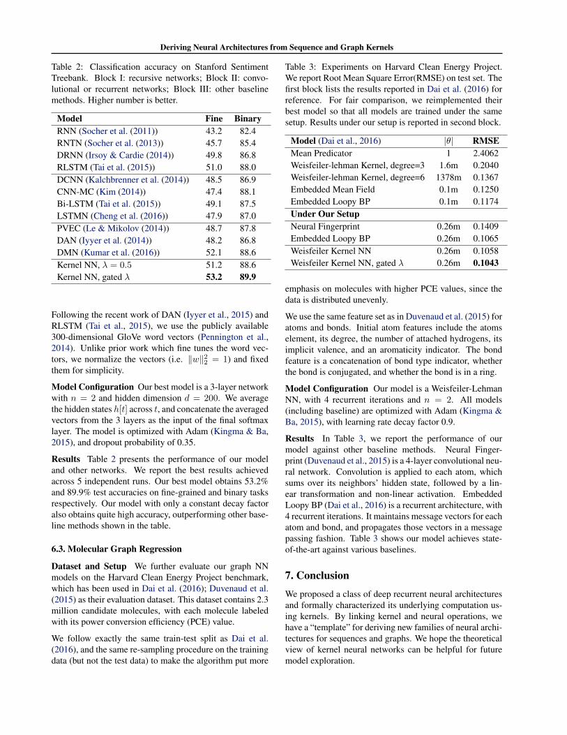
Table 2: Classification accuracy on Stanford SentimentTreebank. Block I: recursive networks; Block II: convo-lutional or recurrent networks; Block III: other baselinemethods. Higher number is better.

Model Fine BinaryRNN (Socher et al. (2011)) 43.2 82.4RNTN (Socher et al. (2013)) 45.7 85.4DRNN (Irsoy & Cardie (2014)) 49.8 86.8RLSTM (Tai et al. (2015)) 51.0 88.0DCNN (Kalchbrenner et al. (2014)) 48.5 86.9CNN-MC (Kim (2014)) 47.4 88.1Bi-LSTM (Tai et al. (2015)) 49.1 87.5LSTMN (Cheng et al. (2016)) 47.9 87.0PVEC (Le & Mikolov (2014)) 48.7 87.8DAN (Iyyer et al. (2014)) 48.2 86.8DMN (Kumar et al. (2016)) 52.1 88.6Kernel NN, λ = 0.5 51.2 88.6Kernel NN, gated λ 53.2 89.9

Following the recent work of DAN (Iyyer et al., 2015) andRLSTM (Tai et al., 2015), we use the publicly available300-dimensional GloVe word vectors (Pennington et al.,2014). Unlike prior work which fine tunes the word vec-tors, we normalize the vectors (i.e. ‖w‖22 = 1) and fixedthem for simplicity.

Model Configuration Our best model is a 3-layer networkwith n = 2 and hidden dimension d = 200. We averagethe hidden states h[t] across t, and concatenate the averagedvectors from the 3 layers as the input of the final softmaxlayer. The model is optimized with Adam (Kingma & Ba,2015), and dropout probability of 0.35.

Results Table 2 presents the performance of our modeland other networks. We report the best results achievedacross 5 independent runs. Our best model obtains 53.2%and 89.9% test accuracies on fine-grained and binary tasksrespectively. Our model with only a constant decay factoralso obtains quite high accuracy, outperforming other base-line methods shown in the table.

6.3. Molecular Graph Regression

Dataset and Setup We further evaluate our graph NNmodels on the Harvard Clean Energy Project benchmark,which has been used in Dai et al. (2016); Duvenaud et al.(2015) as their evaluation dataset. This dataset contains 2.3million candidate molecules, with each molecule labeledwith its power conversion efficiency (PCE) value.

We follow exactly the same train-test split as Dai et al.(2016), and the same re-sampling procedure on the trainingdata (but not the test data) to make the algorithm put more

Table 3: Experiments on Harvard Clean Energy Project.We report Root Mean Square Error(RMSE) on test set. Thefirst block lists the results reported in Dai et al. (2016) forreference. For fair comparison, we reimplemented theirbest model so that all models are trained under the samesetup. Results under our setup is reported in second block.

Model (Dai et al., 2016) |θ| RMSEMean Predicator 1 2.4062Weisfeiler-lehman Kernel, degree=3 1.6m 0.2040Weisfeiler-lehman Kernel, degree=6 1378m 0.1367Embedded Mean Field 0.1m 0.1250Embedded Loopy BP 0.1m 0.1174Under Our SetupNeural Fingerprint 0.26m 0.1409Embedded Loopy BP 0.26m 0.1065Weisfeiler Kernel NN 0.26m 0.1058Weisfeiler Kernel NN, gated λ 0.26m 0.1043

emphasis on molecules with higher PCE values, since thedata is distributed unevenly.

We use the same feature set as in Duvenaud et al. (2015) foratoms and bonds. Initial atom features include the atomselement, its degree, the number of attached hydrogens, itsimplicit valence, and an aromaticity indicator. The bondfeature is a concatenation of bond type indicator, whetherthe bond is conjugated, and whether the bond is in a ring.

Model Configuration Our model is a Weisfeiler-LehmanNN, with 4 recurrent iterations and n = 2. All models(including baseline) are optimized with Adam (Kingma &Ba, 2015), with learning rate decay factor 0.9.

Results In Table 3, we report the performance of ourmodel against other baseline methods. Neural Finger-print (Duvenaud et al., 2015) is a 4-layer convolutional neu-ral network. Convolution is applied to each atom, whichsums over its neighbors’ hidden state, followed by a lin-ear transformation and non-linear activation. EmbeddedLoopy BP (Dai et al., 2016) is a recurrent architecture, with4 recurrent iterations. It maintains message vectors for eachatom and bond, and propagates those vectors in a messagepassing fashion. Table 3 shows our model achieves state-of-the-art against various baselines.

7. ConclusionWe proposed a class of deep recurrent neural architecturesand formally characterized its underlying computation us-ing kernels. By linking kernel and neural operations, wehave a “template” for deriving new families of neural archi-tectures for sequences and graphs. We hope the theoreticalview of kernel neural networks can be helpful for futuremodel exploration.

Deriving Neural Architectures from Sequence and Graph Kernels

AcknowledgementWe thank Prof. Le Song for sharing Harvard Clean En-ergy Project dataset. We also thank Yu Zhang, Vikas Garg,David Alvarez, Tianxiao Shen, Karthik Narasimhan andthe reviewers for their helpful comments. This work wassupported by the DARPA Make-It program under contractARO W911NF-16-2-0023.

ReferencesAnselmi, Fabio, Rosasco, Lorenzo, Tan, Cheston, and Pog-

gio, Tomaso. Deep convolutional networks are hierarchi-cal kernel machines. preprint arXiv:1508.01084, 2015.

Balduzzi, David and Ghifary, Muhammad. Strongly-typedrecurrent neural networks. In Proceedings of 33th In-ternational Conference on Machine Learning (ICML),2016.

Bruna, Joan, Zaremba, Wojciech, Szlam, Arthur, and Le-Cun, Yann. Spectral networks and locally connected net-works on graphs. arXiv preprint arXiv:1312.6203, 2013.

Cheng, Jianpeng, Dong, Li, and Lapata, Mirella. Longshort-term memory networks for machine reading. Pro-ceedings of the Conference on Empirical Methods inNatural Language Processing, pp. 551–562, 2016.

Cho, Youngmin and Saul, Lawrence K. Kernel methods fordeep learning. In Bengio, Y., Schuurmans, D., Lafferty,J. D., Williams, C. K. I., and Culotta, A. (eds.), Advancesin Neural Information Processing Systems 22, pp. 342–350. 2009.

Chung, Junyoung, Gulcehre, Caglar, Cho, KyungHyun,and Bengio, Yoshua. Empirical evaluation of gated re-current neural networks on sequence modeling. arXivpreprint arXiv:1412.3555, 2014.

Dai, Hanjun, Dai, Bo, and Song, Le. Discriminative em-beddings of latent variable models for structured data.arXiv preprint arXiv:1603.05629, 2016.

Daniely, Amit, Frostig, Roy, and Singer, Yoram. Towarddeeper understanding of neural networks: The power ofinitialization and a dual view on expressivity. CoRR,abs/1602.05897, 2016.

Duvenaud, David K, Maclaurin, Dougal, Iparraguirre,Jorge, Bombarell, Rafael, Hirzel, Timothy, Aspuru-Guzik, Alan, and Adams, Ryan P. Convolutional net-works on graphs for learning molecular fingerprints. InAdvances in neural information processing systems, pp.2224–2232, 2015.

Dyer, Chris, Ballesteros, Miguel, Ling, Wang, Matthews,Austin, and Smith, Noah A. Transition-based depen-dency parsing with stack long short-term memory. InProceedings of the 53rd Annual Meeting of the Associa-tion for Computational Linguistics (Volume 1: Long Pa-pers), Beijing, China, July 2015.

Dyer, Chris, Kuncoro, Adhiguna, Ballesteros, Miguel, andSmith, Noah A. Recurrent neural network grammars. InProceedings of the 2016 Conference of the North Amer-ican Chapter of the Association for Computational Lin-guistics, San Diego, California, June 2016.

Gal, Yarin and Ghahramani, Zoubin. A theoreticallygrounded application of dropout in recurrent neural net-works. In Advances in Neural Information ProcessingSystems 29 (NIPS), 2016.

Gartner, Thomas, Flach, Peter, and Wrobel, Stefan. Ongraph kernels: Hardness results and efficient alterna-tives. In Learning Theory and Kernel Machines, pp.129–143. Springer, 2003.

Greff, Klaus, Srivastava, Rupesh Kumar, Koutnık, Jan, Ste-unebrink, Bas R, and Schmidhuber, Jurgen. Lstm: Asearch space odyssey. arXiv preprint arXiv:1503.04069,2015.

Hazan, Tamir and Jaakkola, Tommi. Steps toward deepkernel methods from infinite neural networks. arXivpreprint arXiv:1508.05133, 2015.

Heinemann, Uri, Livni, Roi, Eban, Elad, Elidan, Gal, andGloberson, Amir. Improper deep kernels. In Proceed-ings of the 19th International Conference on ArtificialIntelligence and Statistics, pp. 1159–1167, 2016.

Henaff, Mikael, Bruna, Joan, and LeCun, Yann. Deepconvolutional networks on graph-structured data. arXivpreprint arXiv:1506.05163, 2015.

Hinton, Geoffrey E, Srivastava, Nitish, Krizhevsky, Alex,Sutskever, Ilya, and Salakhutdinov, Ruslan R. Improvingneural networks by preventing co-adaptation of featuredetectors. arXiv preprint arXiv:1207.0580, 2012.

Hochreiter, Sepp and Schmidhuber, Jurgen. Long short-term memory. Neural computation, 9(8):1735–1780,1997.

Irsoy, Ozan and Cardie, Claire. Deep recursive neural net-works for compositionality in language. In Advances inNeural Information Processing Systems, 2014.

Iyyer, Mohit, Boyd-Graber, Jordan, Claudino, Leonardo,Socher, Richard, and Daume III, Hal. A neural net-work for factoid question answering over paragraphs. In

Deriving Neural Architectures from Sequence and Graph Kernels

Proceedings of the 2014 Conference on Empirical Meth-ods in Natural Language Processing (EMNLP), pp. 633–644, Doha, Qatar, October 2014.

Iyyer, Mohit, Manjunatha, Varun, Boyd-Graber, Jordan,and Daume III, Hal. Deep unordered composition rivalssyntactic methods for text classification. In Proceedingsof the 53rd Annual Meeting of the Association for Com-putational Linguistics (Volume 1: Long Papers), 2015.

Kalchbrenner, Nal, Grefenstette, Edward, and Blunsom,Phil. A convolutional neural network for modelling sen-tences. In Proceedings of the 52th Annual Meeting of theAssociation for Computational Linguistics, 2014.

Kim, Yoon. Convolutional neural networks for sentenceclassification. In Proceedings of the Empiricial Methodsin Natural Language Processing (EMNLP 2014), 2014.

Kim, Yoon, Jernite, Yacine, Sontag, David, and Rush,Alexander M. Character-aware neural language mod-els. Twenty-Ninth AAAI Conference on Artificial Intelli-gence, 2015.

Kingma, Diederik P and Ba, Jimmy Lei. Adam: A methodfor stochastic optimization. In International Conferenceon Learning Representation, 2015.

Kumar, Ankit, Irsoy, Ozan, Ondruska, Peter, Iyyer, Mo-hit, James Bradbury, Ishaan Gulrajani, Zhong, Victor,Paulus, Romain, and Socher, Richard. Ask me any-thing: Dynamic memory networks for natural languageprocessing. 2016.

Le, Quoc and Mikolov, Tomas. Distributed representationsof sentences and documents. In Proceedings of the 31stInternational Conference on Machine Learning (ICML-14), pp. 1188–1196, 2014.

Lee, Kenton, Levy, Omer, and Zettlemoyer, Luke. Recur-rent additive networks. Preprint, 2017.

Lei, Tao, Joshi, Hrishikesh, Barzilay, Regina, Jaakkola,Tommi, Tymoshenko, Katerina, Moschitti, Alessan-dro, and Marquez, Lluis. Semi-supervised ques-tion retrieval with gated convolutions. arXiv preprintarXiv:1512.05726, 2015.

Li, Yujia, Tarlow, Daniel, Brockschmidt, Marc, and Zemel,Richard. Gated graph sequence neural networks. arXivpreprint arXiv:1511.05493, 2015.

Lodhi, Huma, Saunders, Craig, Shawe-Taylor, John, Cris-tianini, Nello, and Watkins, Chris. Text classificationusing string kernels. Journal of Machine Learning Re-search, 2(Feb):419–444, 2002.

Merity, Stephen, Xiong, Caiming, Bradbury, James, andSocher, Richard. Pointer sentinel mixture models. arXivpreprint arXiv:1609.07843, 2016.

Pennington, Jeffrey, Socher, Richard, and Manning,Christopher D. Glove: Global vectors for word repre-sentation. volume 12, 2014.

Press, Ofir and Wolf, Lior. Using the output embed-ding to improve language models. arXiv preprintarXiv:1608.05859, 2016.

Ramon, Jan and Gartner, Thomas. Expressivity versus effi-ciency of graph kernels. In First international workshopon mining graphs, trees and sequences, pp. 65–74. Cite-seer, 2003.

Shalev-Shwartz, Shai, Shamir, Ohad, and Sridharan,Karthik. Learning kernel-based halfspaces with the 0-1 loss. SIAM Journal on Computing, 40(6):1623–1646,2011.

Shervashidze, Nino, Schweitzer, Pascal, Leeuwen, ErikJan van, Mehlhorn, Kurt, and Borgwardt, Karsten M.Weisfeiler-lehman graph kernels. Journal of MachineLearning Research, 12(Sep):2539–2561, 2011.

Socher, Richard, Pennington, Jeffrey, Huang, Eric H,Ng, Andrew Y, and Manning, Christopher D. Semi-supervised recursive autoencoders for predicting senti-ment distributions. In Proceedings of the Conference onEmpirical Methods in Natural Language Processing, pp.151–161, 2011.

Socher, Richard, Perelygin, Alex, Wu, Jean, Chuang, Ja-son, Manning, Christopher D., Ng, Andrew Y., and Potts,Christopher. Recursive deep models for semantic com-positionality over a sentiment treebank. In Proceedingsof the 2013 Conference on Empirical Methods in NaturalLanguage Processing, pp. 1631–1642, October 2013.

Srivastava, Rupesh K, Greff, Klaus, and Schmidhuber,Jurgen. Training very deep networks. In Advances inneural information processing systems, pp. 2377–2385,2015.

Tai, Kai Sheng, Socher, Richard, and Manning, Christo-pher D. Improved semantic representations from tree-structured long short-term memory networks. In Pro-ceedings of the 53th Annual Meeting of the Associationfor Computational Linguistics, 2015.

Tamar, Aviv, Levine, Sergey, Abbeel, Pieter, Wu, Yi, andThomas, Garrett. Value iteration networks. In Advancesin Neural Information Processing Systems, pp. 2146–2154, 2016.

Deriving Neural Architectures from Sequence and Graph Kernels

Vishwanathan, S Vichy N, Schraudolph, Nicol N, Kondor,Risi, and Borgwardt, Karsten M. Graph kernels. Jour-nal of Machine Learning Research, 11(Apr):1201–1242,2010.

Zaremba, Wojciech, Sutskever, Ilya, and Vinyals, Oriol.Recurrent neural network regularization. arXiv preprintarXiv:1409.2329, 2014.

Zhang, Yuchen, Lee, Jason D., and Jordan, Michael I. `1-regularized neural networks are improperly learnable inpolynomial time. In Proceedings of the 33nd Interna-tional Conference on Machine Learning, 2016.

Zilly, Julian Georg, Srivastava, Rupesh Kumar, Koutnık,Jan, and Schmidhuber, Jurgen. Recurrent Highway Net-works. arXiv preprint arXiv:1607.03474, 2016.

Zoph, Barret and Le, Quoc V. Neural architecturesearch with reinforcement learning. arXiv preprintarXiv:1611.01578, 2016.

Supplementary Material

A. Examples of kernel / neural variantsOur theoretical results apply to some other variants of sequence kernels and the associated neural compo-nents. We give some examples in the this section. Table 4 shows three network variants, correspondingto three realizations of string kernels provided in Table 5.

Connection to LSTMs Interestingly, many recent work has reached similar RNN architecturesthrough empirical exploration. For example, Greff et al. (2015) found that simplifying LSTMs, by re-moving the input gate or coupling it with the forget gate does not significantly change the performance.However, the forget gate (corresponding to the decay factor λ in our notation) is crucial for performance.This is consistent with our theoretical analysis and the empirical results in Figure 3. Moreover, Balduzzi& Ghifary (2016) and Lee et al. (2017) both suggest that a linear additive state computation suffices toprovide competitive performance compared to LSTMs: 7

c[t] = λf � c1[t− 1] + λi � (Wxt)

h[t] = σ(c[t])

In fact, this variant becomes an instance of the kernel NN presented in this work (with n = 1 and adaptivegating), when λf = λt and λi = 1− λt or 1.

7Balduzzi & Ghifary (2016) also includes the previous token , i.e. Wxt + W′xt−1, which doesn’t affect thediscussion here.

Table 4: Example sequence NN variants. We present these equations in the context of n = 3.

(a) Multiplicative mapping, aggregation un-normalized:

c1[t] = λ · c1[t− 1] +W(1)xt

c2[t] = λ · c2[t− 1] +(c1[t− 1]�W(2)xt

)c3[t] = λ · c3[t− 1] +

(c2[t− 1]�W(3)xt

)

(b) Multiplicative mapping, aggregation normalized:

c1[t] = λ · c1[t− 1] + (1− λ) ·W(1)xt

c2[t] = λ · c2[t− 1] + (1− λ) ·(c1[t− 1]�W(2)xt

)c3[t] = λ · c3[t− 1] + (1− λ) ·

(c2[t− 1]�W(3)xt

)

(c) Additive mapping, aggregation normalized:

c1[t] = λ · c1[t− 1] + (1− λ) ·W(1)xt

c2[t] = λ · c2[t− 1] + (1− λ) ·(c1[t− 1] +W(2)xt

)c3[t] = λ · c3[t− 1] + (1− λ) ·

(c2[t− 1] +W(3)xt

)

Final activation:

h[t] = σ (c3[t])

h[t] = σ (c1[t] + c2[t] + c3[t]) (any linear combination of c∗[t])

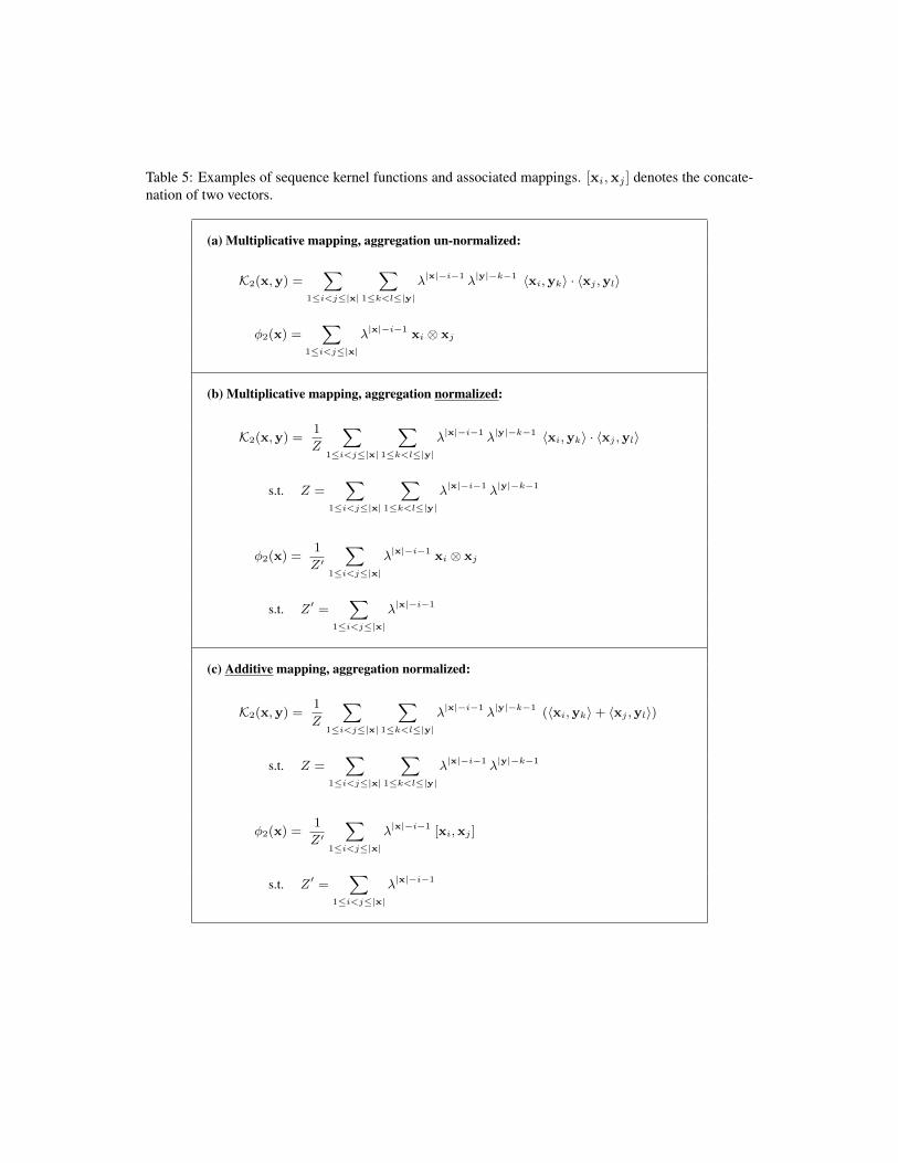
Table 5: Examples of sequence kernel functions and associated mappings. [xi,xj ] denotes the concate-nation of two vectors.

(a) Multiplicative mapping, aggregation un-normalized:

K2(x,y) =∑

1≤i<j≤|x|

∑1≤k<l≤|y|

λ|x|−i−1 λ|y|−k−1 〈xi,yk〉 · 〈xj ,yl〉

φ2(x) =∑

1≤i<j≤|x|

λ|x|−i−1 xi ⊗ xj

(b) Multiplicative mapping, aggregation normalized:

K2(x,y) =1

Z

∑1≤i<j≤|x|

∑1≤k<l≤|y|

λ|x|−i−1 λ|y|−k−1 〈xi,yk〉 · 〈xj ,yl〉

s.t. Z =∑

1≤i<j≤|x|

∑1≤k<l≤|y|

λ|x|−i−1 λ|y|−k−1

φ2(x) =1

Z′

∑1≤i<j≤|x|

λ|x|−i−1 xi ⊗ xj

s.t. Z′ =∑

1≤i<j≤|x|

λ|x|−i−1

(c) Additive mapping, aggregation normalized:

K2(x,y) =1

Z

∑1≤i<j≤|x|

∑1≤k<l≤|y|

λ|x|−i−1 λ|y|−k−1 (〈xi,yk〉+ 〈xj ,yl〉)

s.t. Z =∑

1≤i<j≤|x|

∑1≤k<l≤|y|

λ|x|−i−1 λ|y|−k−1

φ2(x) =1

Z′

∑1≤i<j≤|x|

λ|x|−i−1 [xi,xj ]

s.t. Z′ =∑

1≤i<j≤|x|

λ|x|−i−1

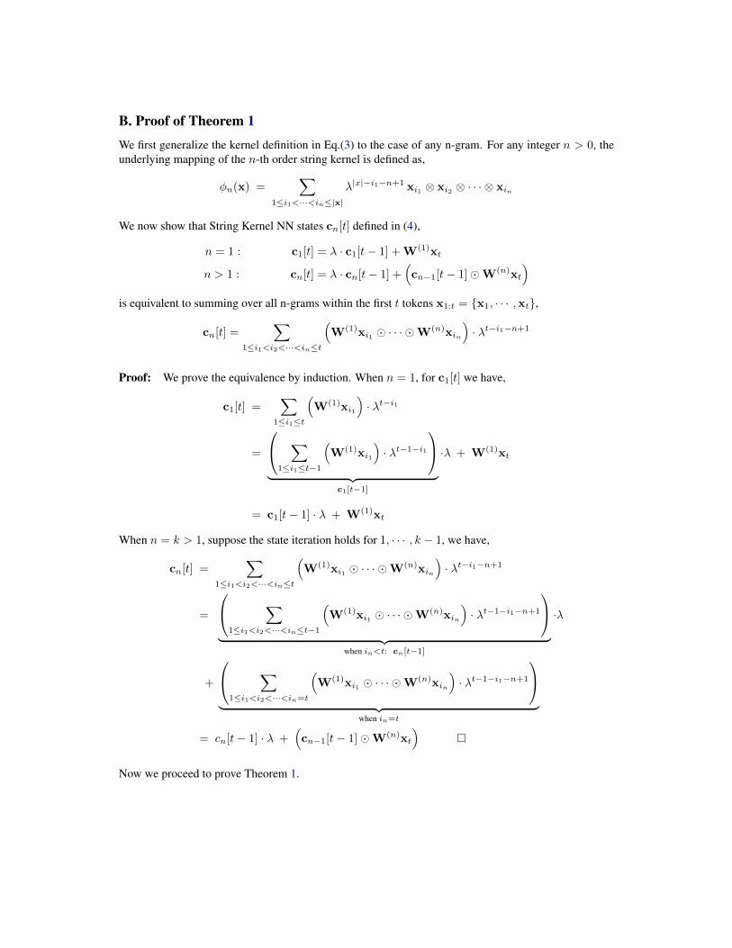
B. Proof of Theorem 1We first generalize the kernel definition in Eq.(3) to the case of any n-gram. For any integer n > 0, theunderlying mapping of the n-th order string kernel is defined as,

φn(x) =∑

1≤i1<···<in≤|x|

λ|x|−i1−n+1 xi1 ⊗ xi2 ⊗ · · · ⊗ xin

We now show that String Kernel NN states cn[t] defined in (4),

n = 1 : c1[t] = λ · c1[t− 1] +W(1)xt

n > 1 : cn[t] = λ · cn[t− 1] +(cn−1[t− 1]�W(n)xt

)is equivalent to summing over all n-grams within the first t tokens x1:t = {x1, · · · ,xt},

cn[t] =∑

1≤i1<i2<···<in≤t

(W(1)xi1 � · · · �W(n)xin

)· λt−i1−n+1

Proof: We prove the equivalence by induction. When n = 1, for c1[t] we have,

c1[t] =∑

1≤i1≤t

(W(1)xi1

)· λt−i1

=

∑1≤i1≤t−1

(W(1)xi1

)· λt−1−i1

︸ ︷︷ ︸

c1[t−1]

·λ + W(1)xt

= c1[t− 1] · λ + W(1)xt

When n = k > 1, suppose the state iteration holds for 1, · · · , k − 1, we have,

cn[t] =∑

1≤i1<i2<···<in≤t

(W(1)xi1 � · · · �W(n)xin

)· λt−i1−n+1

=

∑1≤i1<i2<···<in≤t−1

(W(1)xi1 � · · · �W(n)xin

)· λt−1−i1−n+1

︸ ︷︷ ︸

when in<t: cn[t−1]

·λ

+

∑1≤i1<i2<···<in=t

(W(1)xi1 � · · · �W(n)xin

)· λt−1−i1−n+1

︸ ︷︷ ︸

when in=t

= cn[t− 1] · λ +(cn−1[t− 1]�W(n)xt

)Now we proceed to prove Theorem 1.

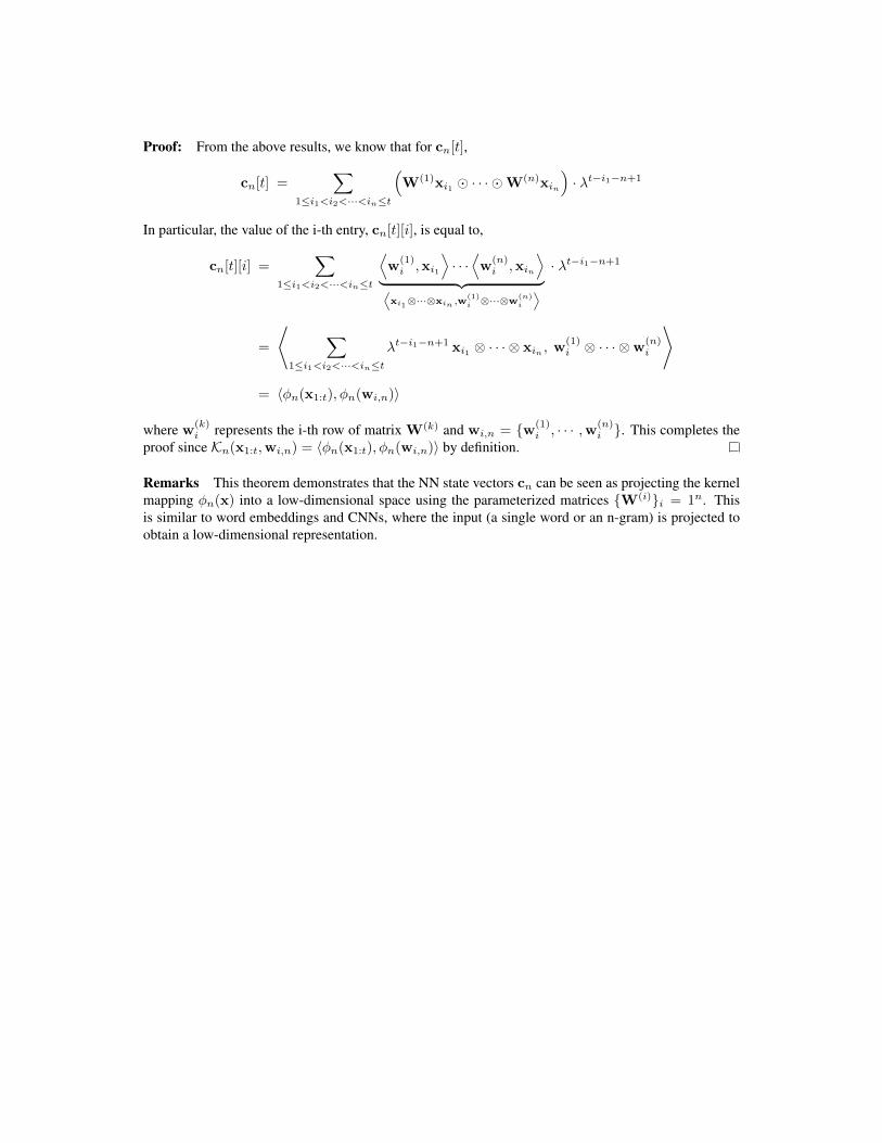
Proof: From the above results, we know that for cn[t],

cn[t] =∑

1≤i1<i2<···<in≤t

(W(1)xi1 � · · · �W(n)xin

)· λt−i1−n+1

In particular, the value of the i-th entry, cn[t][i], is equal to,

cn[t][i] =∑

1≤i1<i2<···<in≤t

⟨w

(1)i ,xi1

⟩· · ·⟨w

(n)i ,xin

⟩︸ ︷︷ ︸⟨

xi1⊗···⊗xin ,w

(1)i ⊗···⊗w

(n)i

⟩· λt−i1−n+1

=

⟨ ∑1≤i1<i2<···<in≤t

λt−i1−n+1 xi1 ⊗ · · · ⊗ xin , w(1)i ⊗ · · · ⊗w

(n)i

⟩

= 〈φn(x1:t), φn(wi,n)〉

where w(k)i represents the i-th row of matrix W(k) and wi,n = {w(1)

i , · · · ,w(n)i }. This completes the

proof since Kn(x1:t,wi,n) = 〈φn(x1:t), φn(wi,n)〉 by definition.

Remarks This theorem demonstrates that the NN state vectors cn can be seen as projecting the kernelmapping φn(x) into a low-dimensional space using the parameterized matrices {W(i)}i = 1n. Thisis similar to word embeddings and CNNs, where the input (a single word or an n-gram) is projected toobtain a low-dimensional representation.

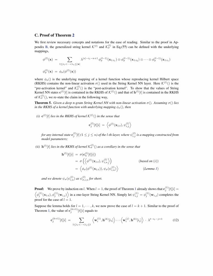
C. Proof of Theorem 2We first review necessary concepts and notations for the ease of reading. Similar to the proof in Ap-pendix B, the generalized string kernel K(l) and K(l)

σ in Eq.(??) can be defined with the underlyingmappings,

φ(l)(x) =∑

1≤i1<···<in≤|x|

λ|x|−i1−n+1 φ(l−1)σ (x1:i1)⊗ φ(l−1)σ (x1:i2)⊗ · · · ⊗ φ(l−1)σ (x1:i1)

φ(l)σ (x) = φσ(φ(l)(x))

where φσ() is the underlying mapping of a kernel function whose reproducing kernel Hilbert space(RKHS) contains the non-linear activation σ() used in the String Kernel NN layer. Here K(l)() is the“pre-activation kernel” and K(l)

σ () is the “post-activation kernel”. To show that the values of StringKernel NN states c(l)[t] is contained in the RKHS of K(l)() and that of h(l)[t] is contained in the RKHSof K(l)

σ (), we re-state the claim in the following way,

Theorem 5. Given a deep n-gram String Kernel NN with non-linear activation σ(). Assuming σ() liesin the RKHS of a kernel function with underlying mapping φσ(), then

(i) c(l)[t] lies in the RKHS of kernel K(l)() in the sense that

c(l)j [t][i] =

⟨φ(l)(x1:t), ψ

(l)i,j

⟩for any internal state c(l)j [t] (1 ≤ j ≤ n) of the l-th layer, where ψ(l)

i,j is a mapping constructed frommodel parameters;

(ii) h(l)[t] lies in the RKHS of kernel K(l)σ () as a corollary in the sense that

h(l)[t][i] = σ(c(l)n [t][i])

= σ(⟨φ(l)(x1:t), ψ

(l)i,n

⟩)(based on (i))

=⟨φσ(φ

(l)(x1:t)), ψσ(ψ(l)i,n)⟩

(Lemma 1)

and we denote ψσ(ψ(l)i,n) as ψ(l)

σ,i,n for short.

Proof: We prove by induction on l. When l = 1, the proof of Theorem 1 already shows that c(1)j [t][i] =⟨φ(1)j (x1:t), φ

(1)j (wi,j)

⟩in a one-layer String Kernel NN. Simply let ψ(1)

i,j = φ(1)j (wi,j) completes the

proof for the case of l = 1.

Suppose the lemma holds for l = 1, · · · , k, we now prove the case of l = k + 1. Similar to the proof ofTheorem 1, the value of c(k+1)

j [t][i] equals to

c(k+1)j [t][i] =

∑1≤i1<···<ij≤t

⟨w

(1)i ,h(k)[i1]

⟩· · ·⟨w

(j)i ,h(k)[ij ]

⟩· λt−i1−j+1 (12)

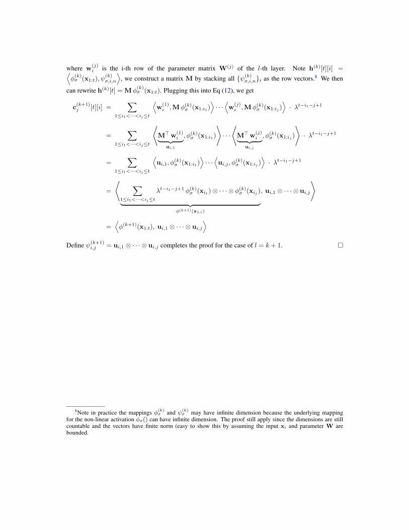
where w(j)i is the i-th row of the parameter matrix W(j) of the l-th layer. Note h(k)[t][i] =⟨

φ(k)σ (x1:t), ψ

(k)σ,i,n

⟩, we construct a matrix M by stacking all {ψ(k)

σ,i,n}i as the row vectors.8 We then

can rewrite h(k)[t] = Mφ(k)σ (x1:t). Plugging this into Eq (12), we get

c(k+1)j [t][i] =

∑1≤i1<···<ij≤t

⟨w

(1)i ,Mφ(k)σ (x1:i1)

⟩· · ·⟨w

(j)i ,Mφ(k)σ (x1:ij )

⟩· λt−i1−j+1

=∑

1≤i1<···<ij≤t

⟨M>w

(1)i︸ ︷︷ ︸

ui,1

, φ(k)σ (x1:i1)

⟩· · ·

⟨M>w

(j)i︸ ︷︷ ︸

ui,j

, φ(k)σ (x1:ij )

⟩· λt−i1−j+1

=∑

1≤i1<···<ij≤t

⟨ui,1, φ

(k)σ (x1:i1)

⟩· · ·⟨ui,j , φ

(k)σ (x1:ij )

⟩· λt−i1−j+1

=

⟨ ∑1≤i1<···<ij≤t

λt−i1−j+1 φ(k)σ (xi1)⊗ · · · ⊗ φ(k)σ (xij )︸ ︷︷ ︸φ(k+1)(x1:t)

, ui,1 ⊗ · · · ⊗ ui,j

⟩

=⟨φ(k+1)(x1:t), ui,1 ⊗ · · · ⊗ ui,j

⟩Define ψ(k+1)

i,j = ui,1 ⊗ · · · ⊗ ui,j completes the proof for the case of l = k + 1.

8Note in practice the mappings φ(k)σ and ψ(k)

σ may have infinite dimension because the underlying mappingfor the non-linear activation φσ() can have infinite dimension. The proof still apply since the dimensions are stillcountable and the vectors have finite norm (easy to show this by assuming the input xi and parameter W arebounded.

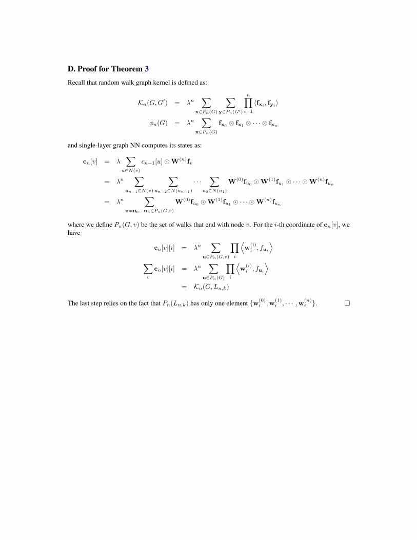
D. Proof for Theorem 3Recall that random walk graph kernel is defined as:

Kn(G,G′) = λn∑

x∈Pn(G)

∑y∈Pn(G′)

n∏i=1

〈fxi , fyi〉

φn(G) = λn∑

x∈Pn(G)

fx0 ⊗ fx1 ⊗ · · · ⊗ fxn

and single-layer graph NN computes its states as:

cn[v] = λ∑

u∈N(v)

cn−1[u]�W(n)fv

= λn∑

un−1∈N(v)

∑un−2∈N(un−1)

· · ·∑

u0∈N(u1)

W(0)fu0 �W(1)fu1 � · · · �W(n)fun

= λn∑

u=u0···un∈Pn(G,v)

W(0)fu0 �W(1)fu1 � · · · �W(n)fun

where we define Pn(G, v) be the set of walks that end with node v. For the i-th coordinate of cn[v], wehave

cn[v][i] = λn∑

u∈Pn(G,v)

∏i

⟨w

(i)i , fui

⟩∑v

cn[v][i] = λn∑

u∈Pn(G)

∏i

⟨w

(i)i , fui

⟩= Kn(G,Ln,k)

The last step relies on the fact that Pn(Ln,k) has only one element {w(0)i ,w

(1)i , · · · ,w(n)

i }.

E. Proof for Theorem 4For clarity, we re-state the kernel definition and theorem in the following:

K(L,n)(G,G′) =∑v

∑v′

K(L,n)loc,σ (v, v

′)

When l = 1:

K(l,j)loc (v, v′) =

〈fv, fv′〉 if j = 1

〈fv, fv′〉+ λ∑

u∈N(v)

∑u′∈N(v′)

K(l,j−1)loc,σ (u, u′) if j > 1

0 if Pj(G, v) = ∅ or Pj(G′, v′) = ∅

When l > 1:

K(l,j)loc (v, v′) =

K(l−1)loc,σ (v, v

′) if j = 1

K(l−1)loc,σ (v, v

′) + λ∑

u∈N(v)

∑u′∈N(v′)

K(l,j−1)loc,σ (u, u′) if j > 1

0 if Pj(G, v) = ∅ or Pj(G′, v′) = ∅

where Pj(G, v) is the set of walks of length j starting from v. Note that we force K(l,j)loc = 0 when there

is no valid walk starting from v or v′, so that it only considers walks of length j. We use additive versionjust for illustration (multiplicative version follows the same argument).

Theorem 6. For a deep random walk kernel NN with L layers and activation function σ(·), assumingthe final output state hG =

∑v h

(l)[v], for l = 1, · · · , L; j = 1, · · · , n:

(i) c(l)j [v][i] as a function of input v and graph G belongs to the RKHS of kernel K(l,j)

loc (·, ·) in that

c(l)j [v][i] =

⟨φ(l,j)G (v), ψ

(l)i,j

⟩where φ(l)G (v) is the mapping of node v in graph G, and ψ(l)

i,j is a mapping constructed from modelparameters.

(ii) h(l)[v][i] belongs to the RKHS of kernel K(l,n)loc,σ(·, ·) as a corollary:

h(l)[v][i] = σ

(∑k

uikc(l)n [v][k]

)= σ

(∑k

uik

⟨φ(l,n)G (v), ψ

(l)k,n

⟩)

= σ

(⟨φ(l,n)G (v),

∑k

uikψ(l)k,n

⟩)

=

⟨φσ(φ

(l,n)G (v)), ψσ

(∑k

uikψ(l)k,n

)⟩

We denote ψσ(∑

k uikψ(l)k,n

)as ψ(l)

σ,i,n, and φσ(φ(l,n)G (v)) as φ(l)G,σ(v) for short.

(iii) hG[i] belongs to the RKHS of kernel K(L,n)(·, ·).

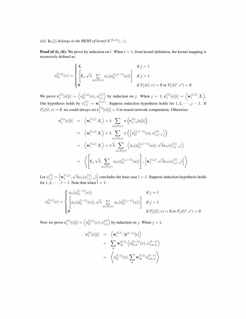
Proof of (i), (ii): We prove by induction on l. When l = 1, from kernel definition, the kernel mapping isrecursively defined as:

φ(1,j)G (v) =

fv if j = 1[fv,√λ

∑u∈N(v)

φσ(φ(1,j−1)G (u))

]if j > 1

0 if Pj(G, v) = ∅ or Pj(G′, v′) = ∅

We prove c(1)j [v][i] =

⟨φ(1,j)G (v), ψ

(1)i,j

⟩by induction on j. When j = 1, c(1)1 [v][i] =

⟨w

(1,1)i , fv

⟩.

Our hypothesis holds by ψ(1)i,1 = w

(1,1)i . Suppose induction hypothesis holds for 1, 2, · · · , j − 1. If

Pj(G, v) = ∅, we could always set c(1)j [v][i] = 0 in neural network computation. Otherwise:

c(1)j [v][i] =

⟨w

(1,j)i , fv

⟩+ λ

∑u∈N(v)

σ(c(1)j−1[u][i]

)=

⟨w

(1,j)i , fv

⟩+ λ

∑u∈N(v)

σ(⟨φ(1,j−1)G (u), ψ

(1)i,j−1

⟩)=

⟨w

(1,j)i , fv

⟩+√λ∑

u∈N(v)

⟨φσ(φ

(1,j−1)G (u)),

√λψσ(ψ

(1)i,j−1)

⟩

=

⟨fv,√λ ∑u∈N(v)

φσ(φ(1,j−1)G (u))

, [w(1,j)i ,

√λψσ(ψ

(1)i,j−1)

]⟩

Let ψ(1)i,j =

[w

(1,j)i ,

√λψσ(ψ

(1)i,j−1)

]concludes the base case l = 1. Suppose induction hypothesis holds

for 1, 2, · · · , l − 1. Note that when l > 1:

φ(l,j)G (v) =

φσ(φ

(l−1)G (v)) if j = 1[

φσ(φ(l−1)G (v)),

√λ

∑u∈N(v)

φσ(φ(l,j−1)G (u))

]if j > 1

0 if Pj(G, v) = ∅ or Pj(G′, v′) = ∅

Now we prove c(l)j [v][i] =

⟨φ(l,j)G (v), ψ

(l)i,j

⟩by induction on j. When j = 1,

c(l)1 [v][i] =

⟨w

(l,1)i ,h(l−1)[v]

⟩=

∑k

w(l,1)ik

⟨φ(l−1)G,σ (v), ψ

(l−1)σ,k,n

⟩=

⟨φ(l,1)G (v),

∑k

w(l,1)ik ψ

(l−1)σ,k,n

⟩

Let ψ(l)i,j =

∑kw

(l,1)ik ψ

(l−1)σ,k,n completes the proof for j = 1. Now suppose this holds for 1, 2, · · · , j − 1.

Same as before, we only consider the case when Pj(G, v) 6= ∅:

c(l)j [v][i] =

⟨w

(l,j)i ,h(l−1)[v]

⟩+ λ

∑u∈N(v)

σ(c(l)j−1[u][i]

)=

∑k

w(l,j)ik

⟨φ(l−1)G,σ (v), ψ

(l−1)σ,k,n

⟩+ λ

∑u∈N(v)

σ(⟨φ(l,j−1)G (u), ψ

(l)i,j−1

⟩)

=

⟨φ(l−1)G,σ (v),

∑k

w(l,j)ik ψ

(l−1)σ,k,n

⟩+ λ

∑u∈N(v)

⟨φ(l,j−1)G,σ (u), ψσ(ψ

(l)i,j−1)

⟩

=

⟨φ(l−1)G,σ (v),

∑k

w(l,j)ik ψ

(l−1)σ,k,n

⟩+

⟨√λ∑

u∈N(v)

φ(l,j−1)G,σ (u),

√λψσ(ψ

(l)i,j−1)

⟩

=

⟨φ(l−1)G,σ (v),√λ∑

u∈N(v)

φ(l,j−1)G,σ (u)

,[∑k

w(l,j)ik ψ

(l−1)σ,k,n ,

√λψσ(ψ

(l)i,j−1)

]⟩

=⟨φ(l,j)G (v), ψ

(l)i,j

⟩Let ψ(l)

i,j =[∑

kw(l,j)ik ψ

(l−1)σ,k,n ,

√λψσ(ψ

(l)i,j−1)

]concludes the proof.

Proof for (iii): We construct a directed chain Ln,k = (V,E) from model parameters, with nodes V =

{ln, ln−1, · · · , l0} and E = {(vi+1, vi)}. lj’s underlying mapping is ψ(L)σ,i,j . Now we have

hG[i] =∑v

h(L)[v][i] =∑v∈G

⟨φσ(φ

(L)G (v)), ψ

(L)σ,i,n

⟩=∑v∈G

∑v∈Ln,k

K(L,n)loc (v, ln) = K(L,n)(G,Ln,k)

Note that we are utilizing the fact that K(L,n)loc (v, lj) = 0 for all j 6= n (because Pn(Ln,j , lj) = ∅).