WP/04/61

Derivative Market Competition: OTC Markets Versus

Organized Derivative Exchanges

Jens Nystedt

© 2004 International Monetary Fund WP/04/61

IMF Working Paper

Policy Development and Review Department

Derivative Market Competition: OTC Markets Versus Organized Derivative Exchanges1

Prepared by Jens Nystedt

Authorized for distribution by Alan MacArthur

April 2004

Abstract

This Working Paper should not be reported as representing the views of the IMF. The views expressed in this Working Paper are those of the author(s) and do not necessarily represent those of the IMF or IMF policy. Working Papers describe research in progress by the author(s) and are published to elicit comments and to further debate.

Recent regulatory initiatives in the United States have again raised the issue of a ''level regulatory and supervisory playing field'' and the degree of competition globally between over-the-counter (OTC) derivatives and organized derivative exchange (ODE) markets. This paper models some important aspects of how an ODE market interrelates with the OTC markets. It analyzes various ways in which an ODE market can respond to competition from the OTC markets and considers whether ODE markets would actually benefit from a more level playing field. Among other factors, such as different transaction costs, different abilitiesto mitigate credit risk play a significant role in determining the degree of competition between the two types of markets. This implies that a potentially important service ODE markets can provide OTC market participants is to extend clearing services to them. Such services would allow the OTC markets to focus more on providing less competitive contracts/innovations and instead customize its contracts to specific investors’ risk preferences and needs. JEL Classification Numbers: F3, G15, G28 Keywords: Derivative market competition, security design, regulatory reform Author’s E-mail Address:

jensnystedt@yahoo.com

1 The author wishes to thank Clas Bergstroem, Bankim Chadha, Peter Englund, Todd Smith, Matthew Spiegel, Staffan Viotti, an anonymous referee, and seminar participants at the International Monetary Fund and the Stockholm School of Economics for helpful comments. Any remaining errors are those of the author.

- 2 -

Contents Page

I. Introduction................................................................................................................4 II. Literature Overview...................................................................................................8 III. The Model..................................................................................................................9 A. Basic Setup.........................................................................................................10 B. The Markets’ Maximization Problems ..............................................................14 IV. Comparative Statics and Model Results ..................................................................25 A. Comparative Statics ...........................................................................................25 B. Additional Model Results ..................................................................................28 V. Analysis and Policy Implications.............................................................................30 VI. Conclusions..............................................................................................................31 Appendix 1. Numerical Examples.................................................................................................33 2. Regulatory and Supervisory Treatment of OTC Versus ODE Derivative in the United States ................................................................................................42 References............................................................................................................................46 Text Tables 1. Definition of Different Derivative Markets ...............................................................5 2. Definition of Key Constants ....................................................................................15 3. Comparative Statics of the Model............................................................................26 Text Figure 1. Evolution of Global Derivatives Market....................................................................6 Appendix Tables A.1 Initial Endowments for Each Agent of the Systematic Asset and the Idiosyncratic Uncorrelated Asset .......................................................................33

- 3 -

Appendix Figures A.1. Optimal ODE Market Transaction Cost.......................................................................34 A.2. Optimal ODE Market Transaction Cost If No Competition ........................................35 A.3. Effect of Changing the Variance of m-risk..................................................................36 A.4. Effect of Changing the Variance of m-risk while allowing TODE to Change...............37 A.5. Effect of Changing Credit Risk Aversion ....................................................................38 A.6. Effect of Changing the Variance of e-risk ...................................................................39 A.7. Effect of Changing the OTC Market’s Risk Aversion.................................................40 A.8. Another look at the effect of Changing Credit Risk Aversion.....................................41

- 4 -

I. INTRODUCTION

"..This is a critical time for all U.S. futures exchanges. Our continued viability is being seriously threatened by two sources of competition—over-the-counter derivatives and foreign futures exchanges."2 "..It is no secret that the combined onslaught of globalization, Over-the-Counter (OTC) competition, and technological advancement, have put enormous pressure on traditional futures exchanges. Indeed in some quarters, there is a growing belief that the good days for traditional exchanges is behind them."3 The recent surge in the use of various forms of financial derivatives globally using various different markets and counterparties highlights the importance of further understanding how different types of derivatives markets compete with and complement each other. This is especially relevant given that most of the spectacular growth seen recently has taken place through an increased usage of OTC (over-the-counter, lightly supervised and self-regulated)

derivatives.4 Many organized derivative exchange markets (liquid, supervised, and regulated) have argued that they are at a comparative disadvantage to OTC derivative markets, highlighting in particular the lack of a level playing field among them owing to differing regulatory and supervisory regimes. From a supervisor's perspective the trend of increased use of OTC derivatives, potentially at the expense of exchange-traded derivatives, raises systemic risk issues given the concentration of OTC derivatives among a few market participants and because these derivatives lack of transparency. Following a string of crises related to the use of OTC derivatives (most recently for Enron, but before that for Long-Term Capital Management, Metallgesellschaft, etc.) the discussion among supervisors has come to focus on whether OTC derivatives should be more closely supervised, regulated, and if investors would have to set aside more capital when trading OTC. This paper analyzes a few aspects of the interrelationship between the organized derivatives exchange markets and the OTC derivatives markets and the degree to which the different markets’ micro structure

2 Patrick H. Arbor, the former Chairman of the Chicago Board of Trade (CBOT). Quotation taken from his testimony before the Risk Management and Specialty Crops Subcommittee of the (U.S.) House Agriculture Committee, April 15, 1997. 3 Speech delivered at the 2000 Canadian Annual Derivatives Conference by Leo Melamed, chairman emeritus of, and senior policy advisor to, the Chicago Mercantile Exchange. 4 OTC markets are by no means unregulated, but rather self-regulated. Industry associations such as International Swaps and Derivative Association (ISDA) provide the OTC markets with standard legal contracts for most types of instruments. This paper assumes, not unreasonably, that this self-regulation gives the OTC market a significant cost advantage over organized exchange markets. For more information, see www.isda.org.

- 5 -

matter. It will also address the issue of whether organized derivative exchange markets actually stand to gain from reducing the OTC market’s risk aversion through various vehicles. Contrary to the highly standardized and usually cleared contracts offered by traditional organized derivative exchange markets (ODEs), OTC derivatives can be individually customized to an end-user's risk preference and tolerance (see Schinasi and others (2000)). Although nearly two-thirds of the actual OTC derivatives traded are of a fairly simple contract structure (for example, a fixed for floating interest rate swap), their terms are still individually determined and highly flexible. An industry group defines OTC derivatives as contracts that are "executed outside of the regulated exchange environment whose values depends on (or derives from) the value of an underlying asset, reference rate or index." 5 6 Clearly, the difference between an ODE derivative and an OTC derivative may concern not only where they are traded but also how. In the United States much attention has been placed on pure OTC derivatives that are privately negotiated between mostly large institutional investors and broker/dealer banks. To ease definitional problems, this paper will focus on some characterized extremes (see Table 1 for definitions).

Table 1. Definition of Different Derivative Markets Standardized Not Standardized

Cleared, regulated ODE markets, such as, CBOE, CBOT, and Eurex.

Tailor-made clearing

Not cleared, self-regulated International Currency and Swap market

Pure OTC derivatives

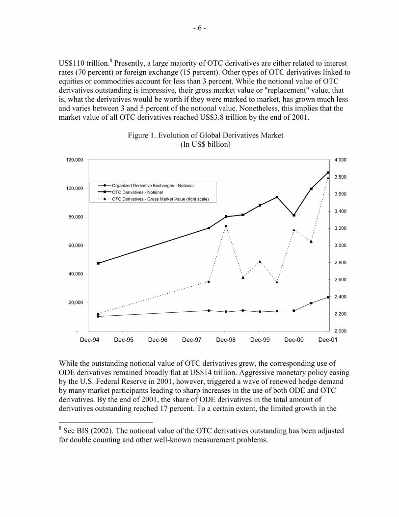
The increased importance of the OTC derivatives market has been a fairly recent phenomenon. By the end of 2001, the size of the global OTC market derivatives was by any measurement huge and growing rapidly (see Figure 1 and BIS (2002)).7 Since the first triennial survey was completed by the Bank for International Settlement (BIS) in 1995, the notional amount of OTC derivatives outstanding (adjusted for double counting) has increased by more than 130 percent, and by the end of 2001 the global amount exceeded 5 Group of Thirty (1993). The Group of Thirty is a group established in 1978, which is a private, nonprofit, international body composed of very senior representatives of the private and public sectors and academia.

6 CFTC (1998).

7 The economic importance of the global derivatives market can not be overstated. As a comparison, as noted in Schinasi and others (2000), world GDP reached US$31 trillion and global net capital flows totaled US$394 billion in 1999.

- 6 -

US$110 trillion.8 Presently, a large majority of OTC derivatives are either related to interest rates (70 percent) or foreign exchange (15 percent). Other types of OTC derivatives linked to equities or commodities account for less than 3 percent. While the notional value of OTC derivatives outstanding is impressive, their gross market value or "replacement" value, that is, what the derivatives would be worth if they were marked to market, has grown much less and varies between 3 and 5 percent of the notional value. Nonetheless, this implies that the market value of all OTC derivatives reached US$3.8 trillion by the end of 2001.

Figure 1. Evolution of Global Derivatives Market (In US$ billion)

-

20,000

40,000

60,000

80,000

100,000

120,000

Dec-94 Dec-95 Dec-96 Dec-97 Dec-98 Dec-99 Dec-00 Dec-012,000

2,200

2,400

2,600

2,800

3,000

3,200

3,400

3,600

3,800

4,000

Organized Derivative Exchanges - NotionalOTC Derivatives - NotionalOTC Derivatives - Gross Market Value (right scale)

While the outstanding notional value of OTC derivatives grew, the corresponding use of ODE derivatives remained broadly flat at US$14 trillion. Aggressive monetary policy easing by the U.S. Federal Reserve in 2001, however, triggered a wave of renewed hedge demand by many market participants leading to sharp increases in the use of both ODE and OTC derivatives. By the end of 2001, the share of ODE derivatives in the total amount of derivatives outstanding reached 17 percent. To a certain extent, the limited growth in the

8 See BIS (2002). The notional value of the OTC derivatives outstanding has been adjusted for double counting and other well-known measurement problems.

- 7 -

notional value of ODE derivatives masks substantial competition between different ODE markets. By now famous examples include the rise of the EUREX market (see Schinasi and others (2000)) at the expense of the LIFFE regarding the trading of futures on German treasury bonds. In general terms, ODE derivatives can be split into two main groups in terms of the notional value outstanding: 90 percent are interest rate derivatives and 9.8 percent are linked to equities. Around 60 percent of these derivatives are traded in the form of options while the remainder consists of futures. Moreover, as pointed out by Cuny (1995), even ODE markets have been highly innovative regarding the launch of new contracts more closely customized to their end users’ needs. While perhaps only a quarter of the new contracts “succeed,” innovation continues to be an important strategy to counter the growth in the use of OTC derivatives. Another strategy is, of course, to strengthen ODE’s market experience and comparative advantage regarding the clearing of transactions, thereby assisting OTC markets in mitigating counterparty credit risk. From a regulator's perspective, the increased clearing of OTC derivatives could help address the concentration of credit risk among the handful of large international banks that today are involved in the vast majority of OTC transactions.9 OTC and ODE derivative markets can both complement and compete with each other. For example, the large broker/dealers of OTC derivatives frequently rely on a liquid ODE market to dynamically hedge their market risk. Conversely, organized futures and derivatives markets in the U.S. face competitive pressure from OTC markets, who are offering fairly similar contracts but are unburdened by regulatory and supervisory oversight. To a certain extent, the competition between OTC derivatives and ODE derivatives is determined by the structure of the contracts and what type of risk the end users would want to hedge. Hence, it may be useful to analyze how ODE markets can increase their comparative advantage in highly standardized and liquid derivatives while also providing clearing services for OTC derivatives. In trying to analyze how ODE markets can respond to the threat posed by OTC derivatives, more research is needed to model these markets' interrelationship. While a potentially relevant area for future regulation initiatives, very little research has been done on this topic.10 Rather, the main focus of the security design literature has been on competition between different stock exchanges or ODE markets. This paper takes a first step to analyze inter-derivative market competition in a multiple contract setting and draws some policy conclusions regarding how competition affects the contracts issued by the two markets, their transaction costs, and whether or not ODE markets would benefit from reducing OTC market risk aversion and investors’ counterparty risk concerns while trading OTC. The main findings of this paper are that the two derivative markets can co-exist in equilibrium while

9 For the second quarter of 2002, seven commercial banks accounted for 96 percent of the total notional amount of derivatives held by the U.S. banking system (estimated at US$50 trillion; see OCC, 2002). OTC derivatives accounted for 90 percent of the total, and the remainder was in the form of ODE contracts. 10 An exception is Kroszner (1999).

- 8 -

exploiting their comparative advantages. Interestingly, the most useful approach for ODE markets to deal with the competitive threat posed by OTC markets is to lower transaction costs, target high variance risks to be hedged, and introduce mechanisms that can help reduce the counterparty credit risk exposure the OTC market faces. This could be achieved, for example, by providing customized clearing services, which would allow the OTC market to better target those investors with particular types of risks. The outline of this paper is as follows. First, a brief literature overview is provided. Second, the modeling section starts with deriving the paper's theoretical framework building on previous work done in the security design literature. In the model, the ODE market can launch only one contract, while the OTC market can launch as many as it wishes. A key contribution is to extend the relatively straightforward innovation modeling framework for the ODE market also to a market with a different structure. After solving for each market’s optimal contract and transaction cost, their effects on trading volume, competition, and risk diversification are analyzed in the second section (a numerical example is provided in the appendix). The section also discusses the degree to which the model takes into account credit risk related costs for the investors and the OTC market, and the effect of this credit risk on market competition. After a discussion of the comparative statics of the model, the follow-on section will discuss some potential policy lessons that could be drawn. The paper ends with some conclusions and ideas for further research. The first appendix discusses some of the model results in the context of various numerical examples, while the second appendix analyzes the United States as an example of some of the regulatory and supervisory challenges facing OTC derivatives compared to ODE derivatives.

II. LITERATURE OVERVIEW

Duffie and Jackson (1989) introduced a useful modeling framework to address issues of optimal financial innovations and transaction costs in an incomplete market setting. Innovations are used in this strand of literature as a term to reflect the best additional contract given previous contracts. This contract/innovation/derivative is optimal if it spans as large a part as possible of a beforehand unspanned portion of the incomplete market. In reality, however, markets will always be incomplete, due to risks that can never be hedged by a financial instrument. The original model by Duffie and Jackson has been extended in at least two main directions. Tashjian and Weissman (1995) used the approach to analyze a futures exchange that can launch several contracts and how it affected trading volumes. Clearly, the futures market will always design the next new contract in such a way that it is likely to generate the highest additional revenue for the exchange, i.e., it will target those investors that have the highest unfilled demand for hedge weighed by their risk aversion. Cuny (1995) enhanced the original model by taking into account the role of liquidity in the design of the optimal contract and the effect of competition between multiple exchanges over time. These extensions have been further generalized in a variety of papers as discussed by the useful surveys completed by Duffie (1992) and Duffie and Rahi (1995).

- 9 -

More recent approaches analyzing multiple exchange competition have brought a variety of different modeling frameworks to the concepts of innovations, competition, etc. Santos and Sheinkman (2001), for example, ask whether competition between organized exchanges lead to excessively low standards in terms of the guarantees/collateral traders have to provide to transact. The authors argue that it has been claimed that the nature of market competition triggers a race for the bottom to maximize trading volume by requiring few performance guarantees/collateral. However, Santos and Sheinkman show in the context of a theoretical two period model, which allows for default among traders but not for them to trade in multiple markets, that the use of guarantees/collateral is indeed constrained efficient in a competitive setting. Interestingly a monopolistic exchange would design its securities and guarantees in such a way that actually less collateral is provided. Moreover, the authors argue that the race to the bottom argument is not borne out in empirical research and that the experience with self-regulation is pretty robust with the exception for potentially extreme events (for example, the 1987 stock market crash). Rahi and Zigrand (2004) analyzes the issue of market competition and financial innovation from the point of view of arbitrageurs/speculators. Rather than assuming, as is common in the literature, that exchanges design the innovations/contracts, Rahi and Zigrand argue that profit seeking agents that trade on the exchanges play an important role in the ultimate design of a financial contract. For example, an arbitrageur/speculator is not only interested in potentially hedging some random endowment but also to identify mispricings or provide liquidity and generate trading profits. These arbitrageurs/speculators differ from the typical investor by their ability to trade across multiple exchanges. The authors assume that investors predominantly interested in hedging their endowments are limited to their “local” exchange. The resulting security design game is driven by the arbitrageurs in terms of what assets are available for trading. Hence, the model developed in their paper derives an endogenously incomplete set of financial assets in the context of segmented markets. What is of particular interest is that Rahi and Zigrand’s model explains why many of the financial innovations actually seen in the real world are in many times redundant, i.e., they could have been created through a combination of previously existing assets. This result predominantly reflects the role arbitrageurs/speculators play across markets and their focus on trading profits rather than maximizing trading volume and the socially optimal level of hedge. The more recent approaches have, as discussed above, shed more light on the various aspects on who is responsible for launching the innovation, and whether or not market competition could have potentially less attractive effects. This paper takes the competition dimension in a new direction by analyzing how two different types of derivative exchanges compete and what are some of the tentative policy lessons that can be concluded from some of the model’s implications.

III. THE MODEL

The model developed in this paper will base itself mostly on the Tashjian and Weissman two-period model. New contracts will be of a very stylized form and a zero interest rate is assumed. While the ODE market is limited to one contract and acts as an intermediary for

- 10 -

transactions, the OTC market can issue as many customized contracts as needed as long as it is willing to take the offsetting position to that of the agent. In the original security design literature, short sales presented a problem (see Allen and Gale (1994)), since it allowed all agents to replicate a potentially new contract without costs. The model developed here has no short sale restriction for neither the ODE contract nor the customized OTC contracts. Short sales are allowed as long as all the trading takes place through one of the markets. An important difference between the ODE and OTC market is, however, that the OTC market will hold positions of its own. In game theoretic terms, the model developed represents a game between a single ODE market and a single OTC market. Both markets will simultaneously offer contracts to a group of agents/investors. Risk averse investors (hedgers and speculators depending on their initial risky endowments and risk tolerances) will buy or sell a contract depending on how attractive the contract is. The key difference between the two different contracts is that the OTC contract can be customized to various degrees to hedge an investor's idiosyncratic risk, something the standardized ODE contract cannot do. At the subsequent time period the risky payoffs are realized and the game ends. Note that it is not a zero sum game, but there is a maximum volume that can be traded because the number of agents in the economy and their endowments are finite. The pareto optimal equilibrium is reached by choosing a set of contracts that maximizes transaction volume and hence the amount of risk transferred. However, non-zero transaction costs, the OTC market’s risk aversion, the agents’ credit risk aversion, and the less than perfect competition between the two markets will ensure that global trading volume is less than pareto optimal. Only two markets are analyzed, making the resulting game fairly simple and tractable. Treating the OTC market as a single concentrated marketplace, which makes the decision of what contract to launch at what price is another simplifying assumption. In reality OTC markets (see Schinasi and others, 2000, for a detailed description) are more of a loose global network of large banks, where the vast majority of transactions are conducted between a handful of large participants.

A. Basic Setup

The construction of the basic version of the model will begin with the derivation of the agents' optimal demands for the different markets' contracts. Knowing these demands, they can then be aggregated across all the agents in the economy. These aggregated demands are the central variables in the markets' maximization problems. The motivation for customization being the key difference between the two markets, is that OTC market participants generally view the ability to off-load highly idiosyncratic risks as one of the key advantages of going to the OTC market.11 Moreover, small and medium investors with other

11 Which is indeed the most frequently cited reason to use the OTC markets, the OCC attributes the rapid growth in OTC derivatives to "banks clients' increasing use of customized solutions for risk management problems" (OCC, 1999).

- 11 -

transactional motives play, even on the ODE markets, a very small role.12 There are, of course, a number of additional market differences that are relevant, such as the ability to transact in relative anonymity on ODE markets, while the regulatory oversight and potential capital charges can be lower with transactions on OTC markets. These considerations, while relevant, are not directly addressed in this paper. There are, in this model setting, K agents, where each individual agent k has its individual constant risk aversion, rk. An agent is endowed, in some numeraire of consumption goods, with a random number of two risky future payoff vectors (assets) m and ke .13 The first asset is the "systematic" part, m, (with a risky pay-off related to, for example, economy wide risks that all agents could face) and the second part is agent k's "idiosyncratic" risk, ke (with a risky payoff related to, for example, non hedgeable basis risk or exposure to individual risks not common with other agents). Here, m

kx denotes the endowment of risky asset m, for a given agent k, and e

kx is the endowment of risky asset ke . Systematic risks and idiosyncratic risks are assumed to be uncorrelated. The total endowment for an agent is equal to:

kek

mkk exmxx +=

The variance of this endowment is: )()()()()()()( 22

kek

mkk

ek

mkk eVarxmVarxexVarmxVarxVar +=+= (1)

For simplicity, it is assumed that the variance of the idiosyncratic risks are the same across agents, i.e., )( keVar is equal to )(eVar and ),( ji eeCov is equal to zero. Risk averse agent k has the choice of hedging his initial risky endowments by buying or selling the ODE derivative contract, with the random payoff ODEf , and/or the OTC derivative, with random payoff OTCkf , . The amounts agent k chooses to buy or sell, are denoted by ODEky , and OTCky , . For each unit he buys or sells in the ODE market he has to pay a transaction cost of ODET . The OTC market does not charge a transaction cost as such, but rather generates revenues from the price offered to the agent (in the form of a bid/ask spread depending on whether the agent is buying or selling). Hence, the price agent k has to pay or receive are determined in equilibrium and are denoted by ODEP and OTCkP , . Since the OTC

12 They constitute about 4 percent of volume traded on NYSE. Their insignificant presence is also valid on the major derivative exchanges (not agricultural commodities though). 13 As is standard in the literature, and for simplicity, we assume that there is no initial endowment of some non-risky asset.

- 12 -

contract is customized for each individual agent it can be broken into its constituent parts, i.e., the risks that are being hedged against. Hence, it assumed that e

OTCkmOTCkOTCk fff ,,, +=

and that the agents demand for the OTC contracts is eOTCk

mOTCkOTCk yyy ,,, += at a price of

eOTCk

mOTCkOTCk PPP ,,, += . Given the presence of two financial markets, agent k is maximizing

his utility by maximizing the next periods' payoff taking into account his risk aversion in the form of a mean variance type utility function subject to some individual level of risk aversion and with normally distributed payoffs.14 To capture an important difference between OTC markets and ODE markets and the fact that transactions in the ODE market are cleared, agents that transact in the OTC market face additional credit risk aversion kc for the exposure they face towards the OTC counterparty

)()()()( OTCkkkkkkk wVarcwVarrwExU −−=

Agent k’s maximization function is hence constructed by substituting k’s pay-off function, i.e., kw , into the utility function. ))()((max ,,,,,, ,,

ODEODEkOTCkOTCkOTCkODEODEODEkkkyyTyPfyPfyxU

OTCkODEk

−−+−+ (2)

Plugging (2) into the agent's mean-variance utility expression, the optimal demand of each contract will depend on how well the contract's payoff hedges k's risky endowment, which is determined by the contract's covariance. In the case of the ODE market, its contract can, by assumption only, hedge the systematic risk, which means that:

0),( =ODEkek fexCov

),(),( ODE

mkODEk fmxCovfxCov =

After some derivation, the optimal volume bought or sold by a certain agent k in market ODE is equal to:15

14 Maximizing a standard mean variance utility function with normally distributed pay-offs is equivalent to maximizing a negative exponential utility function exhibiting constant absolute risk aversion. 15 The derivation of the individual’s optimal volume is relatively straightforward and more details are provided by Tashjian and Weissman (1995) or Duffie and Jackson (1989). As is standard in the literature, no specific budget constraint is assumed in period 0 and agents do not default on their future payment. For a relaxation of the latter assumption please see Santos and Scheinkman (2001).

- 13 -

+−+

−−=

ODEODEkODEODE

mOTCODE

mOTCkkODE

mkk

ODEkODEk TPfE

ffCovyrfmxCovrfVarr

y,

,, )(

),(2),(2)(2

1α (3)

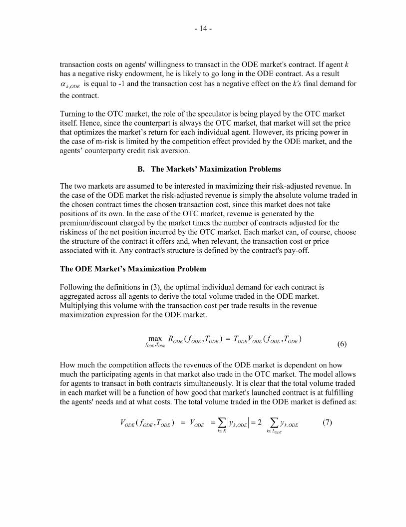
Similarly, the amount bought and sold of the OTC contract addressing m-risk can be expressed by the below expression:

−+

−−

+=

mOTC

mOTC

mOTCODEODEkk

mOTC

mkk

mOTCkk

mOTCk

PfE

ffCovyrfmxCovrfVarcr

y)(

),(2),(2)()(2

1 ,, (4)

While the demand for OTC contract hedging an individual’s idiosyncratic risk can be shown to equal:

[ ]e

OTCkeOTCk

eOTCkk

ekke

OTCkkk

eOTCk PfEfexCovr

fVarcry ,,,

,, )(),(2

)()(21

−+−+

= (5)

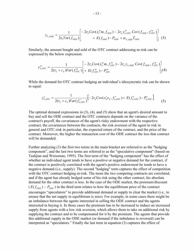
The optimal demand expressions in (3), (4), and (5) show that an agent's desired amount to buy and sell the ODE contract and the OTC contracts depends on the variance of the contract's payoff, the covariances of the agent's risky endowment with the respective contract, the covariances between the contracts, the risk aversion of the agent to risk in general and OTC-risk in particular, the expected return of the contract, and the price of the contract. Moreover, the higher the transaction cost of the ODE contract the less that contract will be demanded. Further analyzing (3) the first two terms in the main bracket are referred to as the "hedging component”, and the last two terms are referred to as the "speculative component" (based on Tashjian and Weissman, 1995). The first term of the “hedging component” has the effect of whether an individual agent tends to have a positive or negative demand for the contract, if the contract is positively correlated with the agent's positive endowment he tends to have a negative demand (i.e., supply). The second "hedging" term captures the effect of competition with the OTC contract hedging m-risk. The more the two competing contracts are correlated, and if the agent has already hedged some of his risk using the other contract, his absolute demand for the other contract is less. In the case of the ODE market, the premium/discount ( ODEODE PfE −)( ) in the third term relates to how the equilibrium price of the contract encourages “speculators” to provide additional demand or supply to clear the market (i.e., to ensure that the net supply in equilibrium is zero). For example, in some cases there might be an imbalance between the agents interested in selling the ODE contract and the agents interested in buying it. In those cases the premium has to be increased to induce an increased supply from agents with a low risk aversion, which allows them to take on additional risk by supplying the contract and to be compensated for it by the premium. The agents that provide this additional supply in the ODE market (or demand if the imbalance is reversed) can be interpreted as “speculators.” Finally the last term in equation (3) captures the effect of

- 14 -

transaction costs on agents' willingness to transact in the ODE market's contract. If agent k has a negative risky endowment, he is likely to go long in the ODE contract. As a result

ODEk ,α is equal to -1 and the transaction cost has a negative effect on the k's final demand for the contract. Turning to the OTC market, the role of the speculator is being played by the OTC market itself. Hence, since the counterpart is always the OTC market, that market will set the price that optimizes the market’s return for each individual agent. However, its pricing power in the case of m-risk is limited by the competition effect provided by the ODE market, and the agents’ counterparty credit risk aversion.

B. The Markets’ Maximization Problems

The two markets are assumed to be interested in maximizing their risk-adjusted revenue. In the case of the ODE market the risk-adjusted revenue is simply the absolute volume traded in the chosen contract times the chosen transaction cost, since this market does not take positions of its own. In the case of the OTC market, revenue is generated by the premium/discount charged by the market times the number of contracts adjusted for the riskiness of the net position incurred by the OTC market. Each market can, of course, choose the structure of the contract it offers and, when relevant, the transaction cost or price associated with it. Any contract's structure is defined by the contract's pay-off. The ODE Market’s Maximization Problem Following the definitions in (3), the optimal individual demand for each contract is aggregated across all agents to derive the total volume traded in the ODE market. Multiplying this volume with the transaction cost per trade results in the revenue maximization expression for the ODE market.

),(),(max, ODEODEODEODEODEODEODETf

TfVTTfRODEODE

= (6)

How much the competition affects the revenues of the ODE market is dependent on how much the participating agents in that market also trade in the OTC market. The model allows for agents to transact in both contracts simultaneously. It is clear that the total volume traded in each market will be a function of how good that market's launched contract is at fulfilling the agents' needs and at what costs. The total volume traded in the ODE market is defined as:

∑∑∈∈

===ODELk

ODEkKk

ODEkODEODEODEODE yyVTfV ,, 2),( (7)

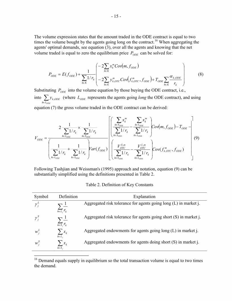
- 15 -

The volume expression states that the amount traded in the ODE contract is equal to two times the volume bought by the agents going long on the contract.16 When aggregating the agents' optimal demands, see equation (3), over all the agents and knowing that the net volume traded is equal to zero the equilibrium price ODEP can be solved for:

( )

( )

+−

−

+=∑∑

∑

∑∈∈

∈

∈Kk k

ODEkODEODE

mOTCk

Kk

mOTCk

ODEKk

mk

Kkk

ODEODE

rTffCovy

fmCovx

rfEP

,,, ,2

,2

/11)( α (8)

Substituting ODEP into the volume equation by those buying the ODE contract, i.e., into ∑

∈ ODELkODEky , (where ODEL represents the agents going long the ODE contract), and using

equation (7) the gross volume traded in the ODE contract can be derived:

( )

−

−−

−

+

×

=

∑∑

∑∑

∑∑

∑∑

∑∑

∈∈

∈

∈

∈

∈

∈∈

∈∈

),(/1/1

,/1/1

)(/1

1/1

1

/11

/112

,

,,

ODEmOTCk

Lkk

mLOTC

Skk

mSOTC

ODEODE

Lkk

Lk

mk

Skk

Sk

mk

ODE

Skk

Lkk

Skk

Lkk

ODE

ffCovr

Vr

V

TfmCovr

x

r

x

fVarrr

rrV

ODEODE

ODE

ODE

ODE

ODE

ODEODE

ODEODE (9)

Following Tashjian and Weissman's (1995) approach and notation, equation (9) can be substantially simplified using the definitions presented in Table 2.

Table 2. Definition of Key Constants

Symbol Definition Explanation Ljγ ∑

∈ jLk kr1

Aggregated risk tolerance for agents going long (L) in market j.

Sjγ ∑

∈ jSk kr1

Aggregated risk tolerance for agents going short (S) in market j.

Ljw ∑

∈ jLkkx Aggregated endowments for agents going long (L) in market j.

Sjw ∑

∈ jSkkx Aggregated endowments for agents doing short (S) in market j.

16 Demand equals supply in equilibrium so the total transaction volume is equal to two times the demand.

- 16 -

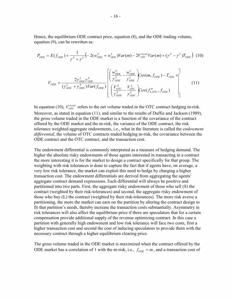
Hence, the equilibrium ODE contract price, equation (8), and the ODE trading volume, equation (9), can be rewritten as:

( )ODELSnetm

OTCLODE

SODELSODEODE TmVarVmVarwwfEP )()(2)()(21)( , γγ

γγ−+−+−

++= (10)

−

+−

−

+=

),(

),(

)()(2

, ODEmOTCkL

ODE

LOTC

SODE

SOTC

ODEODELODE

LODE

SODE

SODE

ODESODE

LODE

SODE

LODE

ODE

ffCovVV

TfmCovww

fVarV

γγ

γγ

γγγγ

(11)

In equation (10), netm

OTCV , refers to the net volume traded in the OTC contract hedging m-risk. Moreover, as stated in equation (11), and similar to the results of Duffie and Jackson (1989), the gross volume traded in the ODE market is a function of the covariance of the contract offered by the ODE market and the m-risk, the variance of the ODE contract, the risk tolerance weighted aggregate endowments, i.e., what in the literature is called the endowment differential, the volume of OTC contracts traded hedging m-risk, the covariance between the ODE contract and the OTC contract, and the transaction cost. The endowment differential is commonly interpreted as a measure of hedging demand. The higher the absolute risky endowments of those agents interested in transacting in a contract the more interesting it is for the market to design a contract specifically for that group. The weighting with risk tolerances is done to capture the fact that if agents have, on average, a very low risk tolerance, the market can exploit this need to hedge by charging a higher transaction cost. The endowment differentials are derived from aggregating the agents' aggregate contract demand expressions. Each differential will always be positive and partitioned into two parts. First, the aggregate risky endowment of those who sell (S) the contract (weighted by their risk-tolerances) and second, the aggregate risky endowment of those who buy (L) the contract (weighted by their risk-tolerances). The more risk averse a partitioning, the more the market can earn on the partition by altering the contract design to fit that partition’s needs, thereby increase the transaction costs substantially. Asymmetry in risk tolerances will also affect the equilibrium price if there are speculators that for a certain compensation provide additional supply of the revenue optimizing contract. In this case a partition with generally high endowment and low risk tolerance will face two costs, first a higher transaction cost and second the cost of inducing speculators to provide them with the necessary contract through a higher equilibrium clearing price. The gross volume traded in the ODE market is maximized when the contract offered by the ODE market has a correlation of 1 with the m-risk, i.e., mfODE = , and a transaction cost of

- 17 -

zero.17 Applying the conclusion regarding the optimal ODE contract into the individual agent’s demand for the ODE contract, equation (3) can be rewritten then be rewritten as:

)(2)( ,

,, mVarrTPfE

yxyk

ODEODEkODEODEmOTCk

mkODEk

α+−+−−=

(12)

As a result, the total volume traded in the ODE market (equation (11)) can be simplified into equation (13).

−

−+

−

+=

)(),(

)(2

,

,,

mVarT

ffCovVVww

V ODEODE

mOTCkL

ODE

LmOTC

SODE

SmOTC

LODE

LODE

SODE

SODE

SODE

LODE

SODE

LODE

ODE γγγγγγγγ

(13)

The variable of choice for the ODE market is, therefore, only the transaction cost that maximizes the ODE market’s revenue. Clearly, trading volume is maximized with a transaction cost of zero, the socially optimal solution if there would be only one market, since risk is shared to the largest extent possible across agents. In a single market setting, the ODE market would, of course not, choose such a transaction cost since its revenue would also be zero. Hence, the ODE market faces the following maximization problem (by substituting equation (13) into equation (6)):

−

−+

−

+ )(),(

)(2

,

,,

mVarT

ffCovVVww

T ODEODE

mOTCkL

ODE

LmOTC

SODE

SmOTC

LODE

LODE

SODE

SODE

SODE

LODE

SODE

LODE

ODEMAXTODE γγγγγγ

γγ (14)

Maximizing equation (14) the ODE market faces a trade-off between the revenues stemming from an increase in the transaction cost and the resulting decrease in trading volume. Moreover, the introduction of inter-market competition results in a particular and new shape to how transaction costs affect a market's revenue. Solving the maximization problems in (14) for the optimal transaction cost yields equation (15).

−+

−= ),(

2)(

,

,,*

ODEmOTCkL

ODE

LmOTC

SODE

SmOTC

LODE

LODE

SODE

SODE

ODE ffCovVVwwmVarTγγγγ

(15)

The optimal transaction costs for the ODE market is increased by a higher variance of the underlying risk it hedges, i.e., given that agents are risk averse they are more willing to pay a higher cost for their hedges. Similarly, the larger the absolute value of the risk weighted endowments of those that trade in the ODE market, the greater the potential for the ODE 17 As stated in Duffie and Jackson (1989), Proposition 1. See the previous table for a definition of the parts of the endowment differential.

- 18 -

market to charge a higher transaction cost. As expected, equation (15) also shows that competition with the OTC contract that hedges m-risk limits the optimal transaction cost charged by the ODE market (since the parenthesis with the volume of OTC contracts traded sums to a negative number). Plugging, the optimal transaction costs into equation (14) generates the following revenue function for the ODE market:

−+

−

+= ),(

)( ,

,,

ODEmOTCkL

ODE

LmOTC

SODE

SmOTC

LODE

LODE

SODE

SODE

SODE

LODE

SODE

LODE

ODEODE ffCovVVww

TRγγγγγγ

γγ (16)

The OTC Market’s Maximization Problem The derivation of the ODE markets revenue function was relatively straightforward, since the ODE market only functions as an intermediary taking no positions of its own and charging an up front transaction cost. However, as shown in equation (16) the ODE markets’ revenue depends on the design of the OTC contract hedging m-risk and the amount that agents already hedge in the OTC market. A key addition of this paper is the introduction of a competing market that has a different structure than the traditional ODE market. As noted earlier, the OTC market will take positions of its own and therefore it is to a certain extent playing a role similar to the speculator in the ODE market case. The OTC market’s objective is to optimize risk-adjusted revenues rather than revenues per se, i.e., it is assumed that the OTC market maximizes a mean-variance type utility function similar to that of the agents, but with risk aversion OTCr . Of course, there is a limit to how much market risk the OTC market can take on. This limit, which could be seen as the maximum value-at-risk an institution is prepared to take, or its net exposure in aggregate to market risk, puts a constraint on how much total risk the OTC market can hedge. Given this constraint the OTC market has an incentive to exploit those agents who have a particular high risk aversion and/or a high level of idiosyncratic risk endowment that can only be hedged through a customized contract. It is, therefore, assumed that the OTC market maximizes the following mean-variance utility function:

)()()( OTCOTCOTCOTCOTC wVarrwEwU −= (17) s.t. Ω≤OTCw

In the above utility expression OTCw expresses the net revenue the OTC market is expected to generate from providing the various contracts to the interested agents. The total market exposure the OTC market can take on is limited by some arbitrary amount Ω . If Ω is sufficiently low compared to hedging demand among the agents the budget constraint will be binding.18 Assuming, that the OTC market offers one contract to hedge agents’ m-risk, and

18 An alternative budget constraint which would be more closely related to a value-at-risk type set up, could be to put an upper limit on the variance of the OTC market’s total market

(continued…)

- 19 -

up to K different customized contracts to hedge an agent’s ke -risk, OTCw would take the following form:

( ) ( )∑∑∈∈

−+−=Kk

eOTCk

eOTCk

eOTCk

Kk

mOTCk

mOTCk

mOTCkOTC fEPyfEPyw )()( ,,,,,, (18)

The OTC market’s maximization problem could be expressed as in equation (19).

( ) ( )

( )

+

−

−−+−=

∑∑

∑∑

∈∈

∈∈

)()(

)()(max

,2

,,

2

,

,,,,,,,,, ,,,,

eOTCk

Kk

eOTCk

mOTCk

Kk

mOTCkOTC

Kk

eOTCk

eOTCk

eOTCk

Kk

mOTCk

mOTCk

mOTCkOTC

ffPP

fVaryfVaryr

fEPyfEPyUe

OTCkm

OTCke

OTCkm

OTCk

(19)

subject to: ( ) ( ) Ω≤−+− ∑∑

∈∈ Kk

eOTCk

eOTCk

eOTCk

Kk

mOTCk

mOTCk

mOTCk fEPyfEPy )()( ,,,,,,

To solve equation (19), a lagrangian function is set up and the lagrange multiplier is used ( kλ ) for agent k, assuming that the budget constraint is binding for the OTC market when supplying a contract to that particular agent. The variance part of equation (19) treats m-risk differently to e-risk. The formulation captures that the OTC market can net out m-risk by taking offsetting positions, but e-risk is individual to each agent and can therefore not be netted similarly. Hence, regarding m-risk it is the net variance that matters for the OTC market. While equation (19) looks fairly complex it can be substantially simplified by carrying over the conclusions regarding the optimal contract design from the ODE market, i.e., the optimal contract is the contract that hedges the agents’ risk the closest.19 This implies that the optimal contracts for the OTC market are given and what remains to do is to solve for the optimal contract prices and the resulting OTC market risk-adjusted revenue.

mff mOTC

mOTCk ==, and k

eOTCk ef =,

It is also assumed that while the idiosyncratic risks and their expected pay-offs would be different across the agents, the variance of these pay-offs would be the same, i.e.:

)()()( , eVareVarfVar keOTCk ==

exposure. Such a limit would, however, unnecessarily complicate the subsequent derivation without much additional insight.

19 This fairly straightforward result was shown in more detail and discussed in an earlier version of this paper, but was left out in the current version for the sake of brevity. The derivation is available from the author upon request.

- 20 -

As a result of these definitions, the demand functions for the OTC contracts, see equations (4) and (5), can be rewritten as:

[ ]m

OTCkm

OTCODEkkkkkk

mOTCk PfEmVaryrmVarxr

mVarcry ,,, )()(2)(2

)()(21

−+−−+

=(4’)

[ ]e

OTCkeOTCk

ekk

kk

eOTCk PfEeVarxr

eVarcry ,,, )()(2

)()(21

−+−+

= (5’)

Substituting the revised demand expressions (including the expression for ODEky , , which is

also a function of mOTCkP , ) into (19), the optimal prices for the OTC market regarding the

contracts mOTCf and e

OTCkf , can be derived.

−

++=

−

++= ∑∈

netmOTC

k

OTCmOTCkk

mOTC

Kk

mOTCk

k

OTCmOTCkk

mOTC

mOTCk

Vr

ycmVarfE

yr

ycmVarfEP

,,

,,,

1)(2)(

1)(2)(

λ

λ (20)

eOTCk

k

OTCkk

eOTCk

eOTCk y

rcreVarfEP ,,, 1

)(2)(

−

+++=λ

(21)

As can be seen from equations (20) and (21), the price the OTC market chooses is basically the expected value of the contract’s pay-off plus a premium/discount, which is directly related to the variance of the underlying risk, the number of contracts bought by the agent, and the agents’ extra risk aversion for trading in an OTC contract. Contrary to the ODE market, where there is one price at which everybody trades, the OTC market can customize its price for each individual agent. In the case of the contract hedging m-risk, the price also reflects the OTC market’s net position. If the demand by agent k reduces the OTC market’s net exposure to m-risk it will quote that agent a more favorable price (last term in equation (20)). Correspondingly, if agent k increases the net exposure of the OTC market, the premium charged to the agent will increase. Due to the competition between the two markets there is an upper bound for the price the OTC market can charge for its m

OTCf contract, which is equal to the price in the ODE market plus the transaction cost ODET . To further exemplify how the OTC market sets the price, consider the case where the OTC market wants to buy an m-risk contract from an agent, the market has to then compensate the agent for the counterparty risk, represented by c , that the agent is assuming by transacting with the OTC market. If the agent would have sold the same

- 21 -

amount of the ODE contract, the counterparty risk would not be present given the clearing function the ODE market provides. The prices of the contracts are also related to the lagrangian kλ when the constraint is binding and reflects the choice of the OTC market of taking on m-risk through the sale or purchase of a contract hedging m-risk or whether it makes more sense for the OTC market to use its finite capacity for market risk to sell or purchase the customized contract hedging the idiosyncratic risk. The relevant lagrangians for the OTC contract hedging m-risk and the one hedging e-risk can be derived by solving (20) and (21) with respect to kλ and setting them equal to each other.20 The revised price for the OTC contract hedging m-risk becomes:

[ ]

+−−++= ))((2)()(2)( ,,

,

,

,, kkeOTCk

eOTCke

OTCk

netmOTCm

OTCkkm

OTCmOTCk creVarfEP

yV

ycmVarfEP (22)

While the price for the e

OTCkf , contract becomes:

( )

−−+++= m

OTCkkm

OTCmOTCknetm

OTCkk

eOTCk

eOTCk

eOTCk ycmVarfEP

VcryeVarfEP ,,,,,, )(2)(1)(2)(

(23) At the point at which the total market exposure constraint Ω is binding, the prices of the contracts offered by the OTC market for a particular agent reflect the potential revenue of instead offering a unit of the alternative contract to that agent or another agent who could generate a higher marginal net revenue (the second term of equation (22) and the third term in the parenthesis of equation (23) could refer to a different agent, which has yet to have its transaction demand satisfied). For example, the OTC market’s pricing decision for the contract hedging m-risk would be affected upwards by the per unit return for the best additional transaction hedging e-risk. An additional effect from supplying an extra contract hedging m-risk at the margin would be that it could lead to a greater risk exposure for which the OTC market would wish to compensate itself for. A similar set of arguments holds for the price of the contract hedging e-risk, when it is being priced in the presence of a binding exposure constraint.

20 The derivation for the kλ s assumes that the OTC market ranks the agents and their demand to transact by the profitability each transaction generates for the market. At some point, i.e., Ω , there is a limit for the OTC market to take on risk. At that limit and for that particular agent affected at that limit, kλ is different from 1 and affects the pricing decision for both the contract hedging m-risk and that hedging e-risk.

- 22 -

Having determined the optimal prices charged by the OTC market for each contract offered to a specific agent, the prices can be substituted into equation (19) for each agent k resulting in the total utility of the OTC market. Also relevant, however, is the amount of m-risk related contracts traded in the OTC market. This amount has to be derived in order to fully understand the driving factors of the market competition and volume traded in the ODE market (see equation (13)). The first step is to substitute the expression for ODEky , into (4’). Together with substituting in the price equation of (20), the new equation is subsequently solved regarding the optimal demand for m

OTCky , :

[ ]ODEODEkODEODEk

netmOTC

kk

OTCmOTCk TPfE

mVarcV

cr

y ,,

, )()(4

12)1(

αλ

+−−−

−= (24)

From equation (10) it is known that the premium/discount for the ODE contract is equal to:

( )ODELSnetm

OTCLODE

SODELS

ODEODEODE

TmVarVmVarww

PfE

)()(2)()(21)(

, γγγγ

−+−+−+

−=

=−=∆

Hence, the net volume traded in the OTC contract hedging m-risk is derived by substituting the above expression into (43), while summing over all agents assuming that those agents buying the ODE contracts would, if they transact at all in the OTC market, also buy m

OTCf contracts.21 The net volume transacted in m

OTCf is equal to: Sm

OTCLm

OTCKk

mOTCk

netmOTC VVyV ,,

,, +== ∑

∈

As shown above, by deriving the volume of those agents buying the m

OTCf contract and selling it, the net volume traded is simply the sum of these two.

( )( ) ∑∑∑

∈∈∈

−∆−

−+−==

OTCmOTCmOTCm Lk k

ODEODE

Lk kk

SmOTC

LmOTC

OTC

Lk

mOTCk

LmOTC cmVar

Tc

VVr

yV,,,

1)(41

1)(2

,,,

,

λ

21 This is not a key assumption, but reduces somewhat the notation necessary to derive the final model. Hence, it is indeed possible that speculators providing much needed liquidity in the ODE market could offset some of their exposure in the OTC market, which would imply that the partitions buying ODE contracts and OTC contracts hedging m-risk are not necessarily the same. Relaxing the assumption would also raise the interesting question of whether speculators in the ODE market are actually hurt by the introduction of an OTC market.

- 23 -

( )( ) ∑∑∑

∈∈∈

+∆−

−+−==

OTCmOTCmOTCm Sk k

ODEODE

Sk kk

SmOTC

LmOTC

OTC

Sk

mOTCk

SmOTC cmVar

Tc

VVr

yV,,,

1)(41

1)(2

,,,

,

λ

)(4)(

)(4)(

)(2

)( ,,,*,*

,

mVarT

mVarVV

rV ODE

SOTC

LOTCODE

SOTC

LOTCSm

OTCLm

OTC

SOTC

LOTCOTCnetm

OTCΓ−Γ

+∆Γ+Γ

−+Γ+Γ

−= (25)

Solving equation (25) for the net volume traded in the OTC contract hedging m-risk, while defining sOTCΓ as the sum of the different buy and sell partitions’ tolerance to OTC credit risk and whether or not the market exposure constraint is binding, the net volume expression can be expressed as in equation (26).22

( )

( )

Γ−Γ+Γ+Γ+−

Π=

Γ−Γ+

+Γ+Γ+−

Γ+Γ+

+Γ+Γ++=

=

ODE

LSOTC

SLOTCS

OTCL

OTCLS

mOTC

ODE

LSOTC

SLOTC

SOTC

LOTC

LS

SOTC

LOTC

LSSOTC

LOTCOTC

LS

netmOTC

TmVar

ww

TmVar

ww

r

V

)()(

)(1

)()(

)(

)(

))(()(21

,*,*

,

γγ

γγγγγγ

(26)

Knowing the net volume traded in the OTC markets allows for the derivation of the gross volume by noting that:

SmOTC

LmOTC

grossmOTC VVV ,,, −=

Similarly, the volume of those buying and selling the OTC contract hedging m-risk has, as previously noted, an impact through the competition dimension on the amount transacted in the ODE contract (see equation (13)). While, a later section will discuss in more detail the key comparative statics of the model conclusions, equation (26) demonstrates that the higher the OTC market’s or the agents’ risk aversions are towards (i.e., the lower the OTC markets risk tolerance, OTCr , the smaller the γ s, and the higher the agents credit risk aversion, kc ) trading OTC contracts the less will be traded OTC and demand is shifted to the ODE market. On the flip side, the higher the transaction cost in the ODE market, the more hedging demand will shift to the OTC market and trigger an increase in trading volume in its m-risk contract. Interestingly, the higher the variance of the underlying risk the lower is the volume traded in the OTC contract hedging m-risk. This is so, since the agents’ aversion towards trading the OTC contract is directly related to the underlying variance and therefore its credit risk.

22 Note that if there is no constraint on the OTC market’s ability to take on risk, or if it is not binding, ,*,* S

OTCL

OTC Γ+Γ would be equal to SOTC

LOTC Γ+Γ .

- 24 -

Hence, a nice result of the model is that it shows that trading on a market where the contracts are cleared and there is no counterparty risk is very attractive for higher risk assets. The total volume traded of e

OTCkf , is much more straightforward to derive, since there is no competition dimension. By substituting the optimal price of the OTC contract hedging e-risk (equation (21) into the agent’s optimal demand expression (equation (5’)) the trading volume in e

OTCkf , would be equal to:

OTCkkk

ekkke

OTCk rcrxr

y++−

−−=

))(1(2)1(

, λλ

The total volume traded in the OTC contract hedging e-risk is derived by simply summing the above expression across all agents23, i.e.,

∑∑

∑∑

∈∈

∈∈

++−−

+++−

−−=

=−=−=

OTCeOTCe

OTCeOTCe

Sk OTCkkk

ekkk

Lk OTCkkk

ekkk

Sk

eOTCk

Lk

eOTCk

SeOTC

LeOTC

eOTC

rcrxr

rcrxr

yyVVV

,,

,,

))(1(2)1(

))(1(2)1(

,,,,

λλ

λλ

(27)

Equation (27) shows the effect of summing individually customized contracts across all the K agents. Given that volume traded by each agent is linked to each individual’s risk and credit risk aversions and endowment of their own idiosyncratic asset it is hard to simplify (26) further. There is a potential intra-OTC market competition dimension, which is related to the constraint on the markets’ total market exposure discussed earlier (the link, for example, affects the price of the contract, see equation (23)). Depending on whether or not the constraint is binding for the marginal OTC contract hedging m-risk or e-risk, a relaxation of the constraint could have an impact on the transaction volume in the ODE market. This relationship is discussed in more detail in the next section. As noted earlier, contrary to the ODE market, the OTC market does not maximize revenue, but risk adjusted utility. Hence, after the optimal prices for the two types of contracts the OTC market offers have been determined and the corresponding transaction volumes, these can be plugged back into the original utility function of equation (19). To reduce notation the variance constraint is assumed not to be binding. This allows the following expression for the utility function of the OTC market.

23 The volume traded is a positive number since those agents’ with a negative endowment tend to buy the OTC derivative, i.e., Le

OTCV , is positive.

- 25 -

( )

+++

+

+

=+=

∑∑∑

∑

∈∈∈

∈

Kk

eOTCkOTC

Kk

eOTCkk

Kk

eOTCkk

netmOTCOTC

Kk

mOTCkk

eOTC

mOTCOTC

yryryceVar

VrycmVar

UUU

2,

2,

2,

2,2,

)()(2)(2)(

)(2)( (28)

IV. COMPARATIVE STATICS AND MODEL RESULTS

An important driving factor in the model is that the OTC contract can also hedge risks that the ODE contract can never address. This asymmetry provides interesting competition questions. For example, what is the volume traded in the ODE market in equilibrium, which market will have the lowest price/transaction cost, and how much does competition increase/lower the socially optimum volume of trading? Since in optimum both markets optimally offer a contract that is perfectly correlated with the underlying risky endowments, the main channel of competition is transaction costs more broadly. As a result, the optimal transaction cost expression for the ODE market has evolved in comparison to the previous literature, while the OTC market competes by price and discrimination between agents.

A. Comparative Statics

Increased competition, through a higher trading volume in the OTC market’s contract hedging m-risk, will decrease the level of the ODE market's optimal transaction cost. Hence, in a non-competitive setting, where there is only one monopolistic financial market providing only contracts hedging m-risk, the optimal transaction cost would be higher (see appendix for some numerical examples). For the OTC market, however, the choice is whether to use its scarce capacity to take on risky positions that are related to m-risk or whether it should only focus on providing a hedge against e-risk. In the model developed in the earlier sections, the OTC market has an obvious advantage in that it can hedge an orthogonal risk that the ODE market can never capture with its contract. Hence, in the absence of competition, the OTC market would provide the optimal contracts for both types of risks. An implication of this competition is that the ODE market's transaction costs, e.g., exchange and clearing fees, have to respond to the presence of a competing market and be reduced. Hence, as a core implication, the ODE market competes, all else being equal, through low transaction costs. However, the relationship between the different markets' transaction costs also depends on the structure of the endowments of the agents. Moreover, in a related decision, the OTC market has to decide to what an extent it wants to act as a “speculator” and take a net positive/negative position in m-risk ( netm

OTCV , ). The fact that it is willing to provide “liquidity” by helping to address any supply/demand imbalances in the endowment of the m-risk asset means that the price at which agents transact in the ODE market actually declines. In the absence of this “speculator” function, the price at which the ODE market clears is higher (if it is assumed that there is a net negative

- 26 -

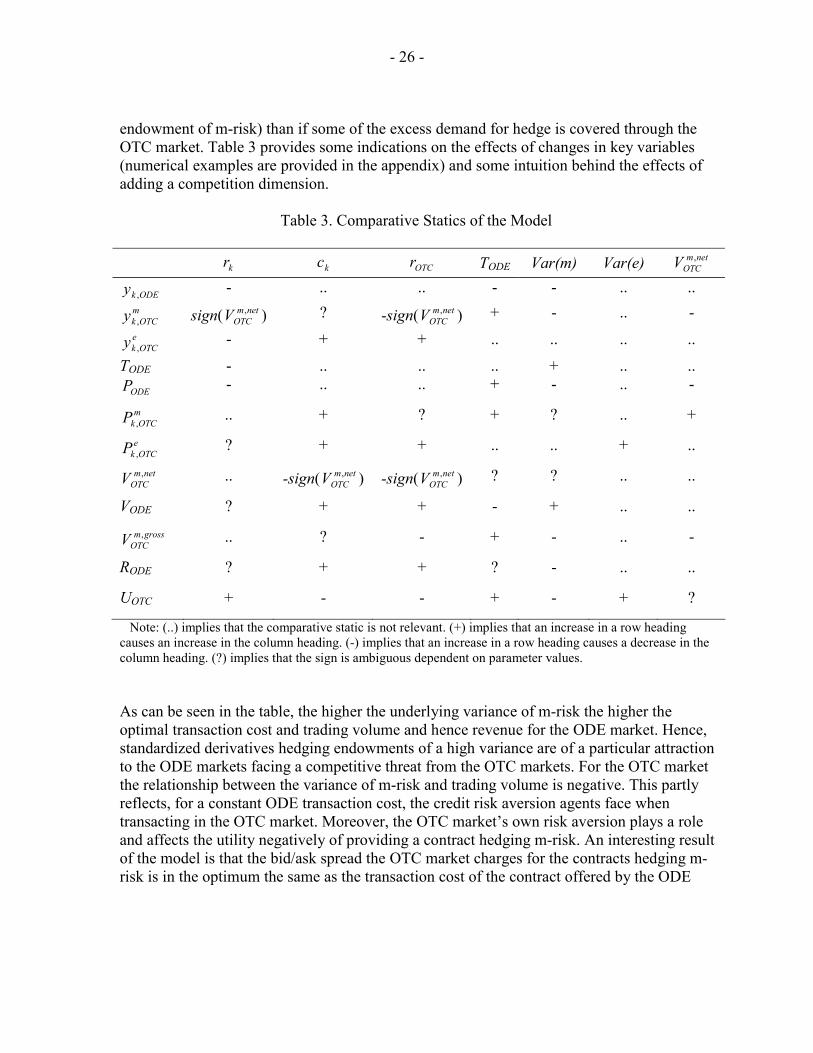
endowment of m-risk) than if some of the excess demand for hedge is covered through the OTC market. Table 3 provides some indications on the effects of changes in key variables (numerical examples are provided in the appendix) and some intuition behind the effects of adding a competition dimension.

Table 3. Comparative Statics of the Model

kr kc OTCr TODE Var(m) Var(e) netm

OTCV ,

ODEky , - .. .. - - .. .. m

OTCky , sign( netmOTCV , ) ? -sign( netm

OTCV , ) + - .. - e

OTCky , - + + .. .. .. ..

TODE - .. .. .. + .. .. ODEP - .. .. + - .. - mOTCkP , .. + ? + ? .. +

eOTCkP , ? + + .. .. + ..

netmOTCV , .. -sign( netm

OTCV , ) -sign( netmOTCV , ) ? ? .. ..

VODE ? + + - + .. .. grossm

OTCV , .. ? - + - .. -

RODE ? + + ? - .. ..

UOTC + - - + - + ?

Note: (..) implies that the comparative static is not relevant. (+) implies that an increase in a row heading causes an increase in the column heading. (-) implies that an increase in a row heading causes a decrease in the column heading. (?) implies that the sign is ambiguous dependent on parameter values. As can be seen in the table, the higher the underlying variance of m-risk the higher the optimal transaction cost and trading volume and hence revenue for the ODE market. Hence, standardized derivatives hedging endowments of a high variance are of a particular attraction to the ODE markets facing a competitive threat from the OTC markets. For the OTC market the relationship between the variance of m-risk and trading volume is negative. This partly reflects, for a constant ODE transaction cost, the credit risk aversion agents face when transacting in the OTC market. Moreover, the OTC market’s own risk aversion plays a role and affects the utility negatively of providing a contract hedging m-risk. An interesting result of the model is that the bid/ask spread the OTC market charges for the contracts hedging m-risk is in the optimum the same as the transaction cost of the contract offered by the ODE

- 27 -

market.24 This assumes that the endowment of the agent trying to sell m-risk and that of the agent buying m-risk is the same with the signs reversed. Also they must have the same risk aversions and the exposure constraint has to be non-binding. Moreover, it can be shown that the bid/ask spread the OTC market will charge in optimum for the contract hedging m-risk is equal to the transaction cost chosen by the ODE market. If there was no competition from the ODE market, however, both the optimal demand for the OTC contract hedging m-risk and the bid/ask spread would be different (see below, modifies equation (24)).

)2)(1(2,,

,kkk

OTCnetmOTC

kk

kmk

nocompmOTCk cr

rV

crr

xy+−

−+

−=λ

If it is assumed that the risk and credit aversions of the agent going long the OTC contract hedging m-risk are the same as those of the agent going short the contract the bid/ask spread in a non-competitive setting is equal to:

( )mL

mS

mOTCS

mOTCL xx

crcmVarPP −

+=−

2)(2

,, where ( ) 0>− mL

mS xx

This bid/ask spread, depending on the gross endowments of the two agents going long versus short can be bigger or smaller than the ODE market optimal transaction cost in a competitive setting. Turning to the variance of e-risk, the effect of a higher variance is the reverse of what it is for the OTC market in terms of m-risk. The intuitive reason for this result is that the OTC market is exploiting its monopoly power as much as possible in the e-risk market. Since it is the sole provider of an instrument to hedge the idiosyncratic risk, it can ask a high price for that service. Of course, a side effect of entering into a lot of fairly rewarding contracts hedging agents’ individual e-risk is that the variance of those positions quickly add up and do not net out in the same sense as the positions the OTC market enters into regarding m-risk (where it is the net position that matters). If the OTC market has a high level of risk aversion it would relatively shift more of its exposure and transaction volume to the contract hedging m-risk than to the contract hedging e-risk. For example, if the OTC market’s risk aversion is very high it can still transact in the m-risk market, while setting its net exposure to zero. Of course, the side effect in this case would be that the equilibrium price charged by the ODE market increases since the OTC market would not play any market maker function by 24 Assume two agents, one that wants to buy the OTC contract hedging m-risk and one that wants to sell the contract. The bid/ask spread is derived by subtracting the price charged by the OTC market to the seller from that charged to the buyer. By substituting in the agents optimal demand/supply it turns out that the optimal bid/ask spread that the OTC market charges is the transaction cost charged by the ODE market. Hence, as the transaction cost in the ODE market is increased it is optimal for the OTC market to follow suit, i.e., doesn’t compete on price.

- 28 -

assuming risk. In this example, the OTC market may therefore be unwilling to transact in any OTC contract hedging e-risk or only at such a high cost that agents do not want to hedge these risks (see the appendix for a quantification of this example). Such an outcome would have fairly large negative welfare effects.

B. Additional Model Results

So far the downside of customization has not been discussed in detail. Customization leads to an accumulation of credit risk, because neither the agents nor the OTC market can normally hedge its credit (or counter party) risk. Accumulating credit risk is clearly costly to the agent and the issuing OTC market. In the case of the ODE market, however, credit risk is dealt with through the clearing system. Agents transacting in the OTC markets do not generally have access to such clearing facilities. Therefore, it is reasonable to assume that in the case of the OTC markets, the more customized a contract is, and the higher the market value of it is, the larger is the subsequent credit risk exposure faced by the agent and the issuer. Customization also limits the possibility of a resale if the counterparty enters default. In the global OTC interest rate and foreign exchange swap markets, recently evolving bilateral and multilateral netting arrangements are potentially an efficient way to decrease the credit risk faced by a single participant. Regardless of the ways in which the agents transacting in the OTC market try to mitigate their credit risk exposure, the maximum possible unhedgeable loss to the agent, i.e., the number of contracts times the contract’s payoff, will be a key variable in the agents’ utility functions. In general agents, as well as the OTC market, have to set aside some amount of capital against their net OTC counterparty exposure (in the case of international banks it would depend on the maximum loss according to the traditional BIS rules). Setting aside capital is costly, since it is not earning as much return as it could. Therefore, credit exposure incurs a cost for the issuing bank or organization. Several ODE markets are starting to offer successful ways to reduce the credit risk costs faced by the OTC markets by offering them tailor made clearing services.25 This fairly recent strategy exploits the ODE markets' long experience with clearing. According to a recent BIS (1998) publication, several additional derivatives exchanges have announced the setting up of clearing facilities for less exotic OTC contracts. In the model developed in this paper, some of the costs of customization are modeled by including the OTC market’s general risk aversion and the agents’ specific individual credit risk aversion, kc . Increased level of credit risk aversion among agents have a direct effect on their demand for the OTC contracts. Given the presence of competition in the case of the

25 Several clearing houses have been recently set up to clear fairly standardized OTC transactions, e.g., Brazil BM&F, Sweden's OM's Tailor Made Clearing, and the London Clearing House's Swapclear. For more information see BIS (1998) and the President's Working Group on Financial Markets (1999).

- 29 -

OTC contract hedging m-risk, a change in the credit risk aversion parameter does not change the OTC market’s optimal bid/ask spread, which is still equal to the ODE market’s transaction cost, but rather affects transaction volume. Similarly, the price spread for agents’ hedging their e-risks, while having similar endowments and risk aversions, is also unchanged. Hence, the transaction demand for OTC contracts is rapidly negatively affected and the effect is especially pronounced for the OTC contracts hedging e-risk, given the higher marginal utility the OTC market, due to its monopoly position derives from this market and perhaps also the higher variance of the e-risk endowment. The ODE market, however, clearly stands to gain from the loss in competitiveness from the OTC market and both ODE market revenue and volume would respond positively. The overall utility of the agents trying to hedge their risks suffers, however, since the positive effect of market competition on prices and transactions costs are eroded. A remaining and related variable to be analyzed is the importance played by the exposure restriction Ω and its interplay with the other key variables, such as risk and credit risk aversion. Equation (19) shows that the OTC market’s ability to expose itself to market risk is limited. Depending on the size of the limit, this restriction will force the OTC market to make a decision between providing OTC contracts hedging m-risk or e-risk. In essence, this constraint implies that the OTC market has to rank each potential transaction by the utility it creates and then select the contracts that provide the highest utility whether they are hedging m or e-risk. If Ω is set high enough, i.e., the constraint is largely non-binding, then

kk ∀= 0λ and the OTC market can maximize freely (as is assumed in the numerical examples in the appendix). The more interesting case is when the constraint is sufficiently binding and the OTC market’s risk aversion is high. In such a scenario, the market is now maximizing within the constraint and will provide mostly contracts hedging m-risk. If, however, the constraint was binding in the context of low OTC market risk aversion, the OTC market would largely only have provided contracts hedging e-risk. These results are, however, largely driven by the assumptions of the associated parameter values of the constraint and the risk aversions, but show that with an assumption of an economically binding constraint, the lower the OTC market’s risk aversion, the more it will provide hedge for those agents with e-risk. This also means that in the case of the ODE market, and as noted in equation (14) and (16) and Table 3, its trading volume and revenue would increase when the risk aversion for the OTC market declines.26 If, however, the risk aversion of the OTC market is very high while the budget constraint is non-binding it is possible that small changes in the risk aversion have no significant impact on the degree of competition with the ODE market. This is the case, when as above, the OTC market decides to take a near net zero position in contracts hedging m-risk. 26 This can be easily seen from a comparative static sense by setting the γ s equal to each other. In that case, the gross volume traded in the OTC contract hedging m-risk directly decreases overall ODE trading volume, optimal transaction cost, and, as a result, ODE revenue.

- 30 -

V. ANALYSIS AND POLICY IMPLICATIONS

The first implication of the model is that by introducing an interrelationship between two different derivative markets changes the behavior of both the ODE market and the OTC market in very fundamental ways. The new contracts launched by each market and their costs have to now take into account the competitor's response. For the ODE market, the optimal contract is still of the classic Duffie and Jackson (1989) type, i.e., strictly geared towards hedging systematic risk. However, the ODE market's optimal transaction cost now reflects a competition dimension. A second implication is that the optimal transaction costs and prices for both markets are critically dependent on the agents' initial endowment structure. Moreover, an ODE market competes preferably with transaction costs, while the OTC market selects to launch an OTC contract hedging m-risk at a price that does not, in optimum, outcompete the ODE market. Hence, in equilibrium, both contracts, which compete regarding their ability to hedge m-risk, will face some demand and both play a useful role in maximizing the transaction volume, lowering monopoly rents, and increase the degree of socially optimal hedging. The model also tries to capture a sense of counterparty credit risk, stemming from the costs of customization, which result in some additional interesting implications. Increased credit risk aversion decreases the demand for customized OTC contracts and reduces the beneficial impact on the agents of introducing competition between markets. Moreover, the interrelationship between the OTC market’s risk aversion and its market exposure constraint is such that a reduction in risk aversion may allow the OTC market to focus more on providing agents with a hedge for their e-risk rather than hedging their m-risk. This leads to an important insight that is not directly captured in the model but is relevant for the real world, i.e., an ODE market has at least three options in responding to the competitive threat posed by the OTC markets, first it can decrease its transactions costs, second it could target only endowments with a very high variance, and third it could make it cheaper for the OTC market to customize OTC instruments by providing efficient clearing services and thereby reducing its overall risk. This implication is in line with the recent initiatives by several ODE markets to introduce tailor made clearing services for some OTC contracts. This means that the rapid growth of OTC markets does not need to necessarily be a threat to those ODE markets that are quick to adapt by providing clearing services and thereby grow with the OTC markets. Kroszner (1999) discusses an alternative mechanism, the so called derivative product company (DPC), through which participants in the OTC markets can limit counterparty risk. DPCs are generally separately capitalized special purpose vehicles with a high credit rating and are set up by one of the international banks. A significant share of the international banks’ OTC transactions are channeled through DPCs, (see Kroszner (1999) for a more detailed discussion), ensuring that any counterparty risk for the bank is with the DPC and that of the end-user is with the DPC as well. While the DPC approach mimics to a certain extent a clearing structure, it does net credit risk exposure for the bank, its main use has been to ensure that international banks with a relatively low rating can still take part in the OTC market through these special purpose vehicles. Hence, the use of DPCs has diminished over the last few years as banks have attained a higher credit rating.

- 31 -

It can further be surmised that any corporate entity could provide clearing services without being in itself an ODE market. Perhaps this is true, but existing ODE markets are likely to both benefit from significant first mover advantages and the fact that clearing is a business with large economies of scale. Hence, there seems to be significant, if increasingly tapped, potential for ODE derivative markets to evolve into clearing specialists, off loading and effectively managing the risks taken by OTC markets. From a supervisory perspective such a development should be rather welcome, since the authorities' main concern has been the systemic stability of the OTC market as a whole (see Schinasi and others, 2000). In the U.S. (see appendix II) voices have recently been raised for the regulation of the OTC markets and the deregulation of the ODE markets. This paper suggests that in addition to trying to deregulate themselves faster, ODE derivatives markets have other avenues to evolve their businesses, and supervisory institutions could ensure that expanding these markets' clearing business is supported through perhaps regulatory incentives.

VI. CONCLUSIONS

The model presented in this paper addresses the issue of the interrelationship between two different markets, the ODE market, and the OTC market. During the last few years, the competition between these markets has grown more intense and ODE markets are actively seeking alternative strategies to come to grips with the OTC markets, such as increased innovation, lower transaction costs, lobbying for the leveling of the regulatory and supervisory playing field, and launching clearing facilities for certain types of OTC contracts. In this paper the main differences between these markets are modeled as, and argued to be, differences in the type of risk they can hedge against, their different risk aversions, and in how they can handle the agents' credit risk. The contracts considered are generally of a forward type that can either hedge systematic risk (m-risk) or an agent’s idiosyncratic risk (e-risk). The modeling framework introduced is an extension of the incomplete markets financial contract model originally developed by Duffie and Jackson (1989). It is argued in the paper that OTC and ODE derivative markets can both complement and compete with each other. For example, the large broker/dealers of OTC derivatives frequently rely on a liquid ODE market to dynamically hedge their market risk. Conversely, organized futures and derivatives markets in the U.S. face competitive pressure from OTC markets, who are offering fairly similar contracts but are unburdened by regulatory and supervisory oversight. To a certain extent, the competition between OTC derivatives and ODE derivatives is determined by the structure of the contracts and what type of risk the end users would want to hedge. Hence, it may be useful to analyze how ODE markets can increase their comparative advantage in highly standardized, high variance, and liquid derivatives while also providing clearing services for OTC derivatives. In trying to analyze how ODE markets can respond to the threat posed by OTC derivatives more research is, of course, needed to model these markets' interrelationships. While a potentially relevant area for future regulation initiatives, very little research has yet been done on this topic. Rather, the main focus of the security design literature has been on competition between different stock exchanges or ODE markets. This paper takes a first step to analyze inter-derivative

- 32 -

market competition in a multiple contract setting. The main findings of this paper are that the two derivative markets can co-exist in equilibrium while exploiting their comparative advantages. Competition is also clearly welfare enhancing and a better outcome for the agents trying to hedge their m or e-risk than in any one market setting. This result is shown to hold true even in a setting where the OTC market can issue multiple contracts, while the ODE market is limited to only one. Interestingly, to decrease competitive pressures, it is sometimes in the ODE markets’ interest to help reduce the OTC market risk aversion. For example, in a U.S. setting (discussed in Appendix II) ODE markets could avoid lending their support to increased regulatory pressure on OTC markets that could increase the cost for the OTC market to offer customized contracts. Instead, the most useful approach for ODE markets to deal with the competitive threat posed by OTC markets could be to lower transaction costs, target high variance assets, and introduce mechanisms that can help reduce the counterparty credit risk the OTC market takes on when transacting with counterparties. This could be achieved, for example, by providing customized clearing services, which would allow the OTC market to better target those investors with particular types of risks. For further research purposes, an empirical paper would be very useful in quantifying some of the assumptions made in this paper. While it is clear that competition between the two market types is intense both in the United States and globally, from the ODE markets’ perspective, there are no studies that compare, for example, transaction costs of similar OTC and ODE derivatives. A part of the explanation for the lack of research in this area is attributed to the difficulty of collecting what are often proprietary transaction data for the OTC markets. In summary, this paper could serve as useful background information for understanding the competitive market microstructure between two different market types that issue 1 to multiple contracts. Hence, it can serve as a first cut at trying to better understand the relationship between these two very important derivative markets and informs the policy discussions about reforming and regulating ODE and OTC markets, especially in the United States, and abroad.

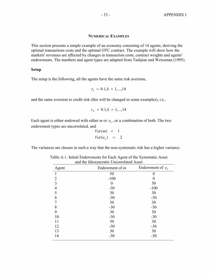
- 33 - APPENDIX I

NUMERICAL EXAMPLES

This section presents a simple example of an economy consisting of 14 agents, deriving the optimal transactions costs and the optimal OTC contract. The example will show how the markets' revenues are affected by changes in transaction costs, contract weights and agents' endowments. The numbers and agent types are adapted from Tashjian and Weissman (1995). Setup The setup is the following, all the agents have the same risk aversion,

14...,,1,1.0 == krk and the same aversion to credit risk (this will be changed in some examples), i.e.,

14...,,1,1.0 == kck Each agent is either endowed with either m or ke , or a combination of both. The two endowment types are uncorrelated, and

2)(1)(

==

keVarmVar

The variances are chosen in such a way that the non-systematic risk has a higher variance.

Table A.1. Initial Endowments for Each Agent of the Systematic Asset and the Idiosyncratic Uncorrelated Asset

Agent Endowment of m Endowment of ke 1 50 0 2 -100 0 3 0 50 4 -30 -100 5 30 30 6 -30 -30 7 30 30 8 -30 -30 9 30 30 10 -30 -30 11 30 30 12 -30 -30 13 30 30 14 -30 -30

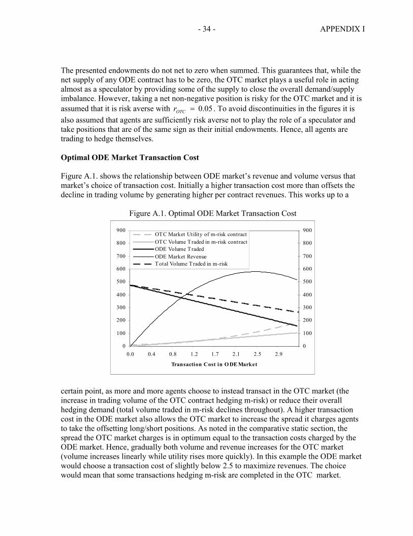
- 34 - APPENDIX I

The presented endowments do not net to zero when summed. This guarantees that, while the net supply of any ODE contract has to be zero, the OTC market plays a useful role in acting almost as a speculator by providing some of the supply to close the overall demand/supply imbalance. However, taking a net non-negative position is risky for the OTC market and it is assumed that it is risk averse with 05.0=OTCr . To avoid discontinuities in the figures it is also assumed that agents are sufficiently risk averse not to play the role of a speculator and take positions that are of the same sign as their initial endowments. Hence, all agents are trading to hedge themselves. Optimal ODE Market Transaction Cost Figure A.1. shows the relationship between ODE market’s revenue and volume versus that market’s choice of transaction cost. Initially a higher transaction cost more than offsets the decline in trading volume by generating higher per contract revenues. This works up to a

Figure A.1. Optimal ODE Market Transaction Cost

0

100

200

300

400

500

600

700

800

900

0.0 0.4 0.8 1.2 1.7 2.1 2.5 2.9

Transaction Cost in O DE Market

0

100

200

300

400

500

600

700

800

900OTC Market Utility of m-risk contractOTC Volume Traded in m-risk contractODE Volume TradedODE Market RevenueTotal Volume Traded in m-risk

certain point, as more and more agents choose to instead transact in the OTC market (the increase in trading volume of the OTC contract hedging m-risk) or reduce their overall hedging demand (total volume traded in m-risk declines throughout). A higher transaction cost in the ODE market also allows the OTC market to increase the spread it charges agents to take the offsetting long/short positions. As noted in the comparative static section, the spread the OTC market charges is in optimum equal to the transaction costs charged by the ODE market. Hence, gradually both volume and revenue increases for the OTC market (volume increases linearly while utility rises more quickly). In this example the ODE market would choose a transaction cost of slightly below 2.5 to maximize revenues. The choice would mean that some transactions hedging m-risk are completed in the OTC market.

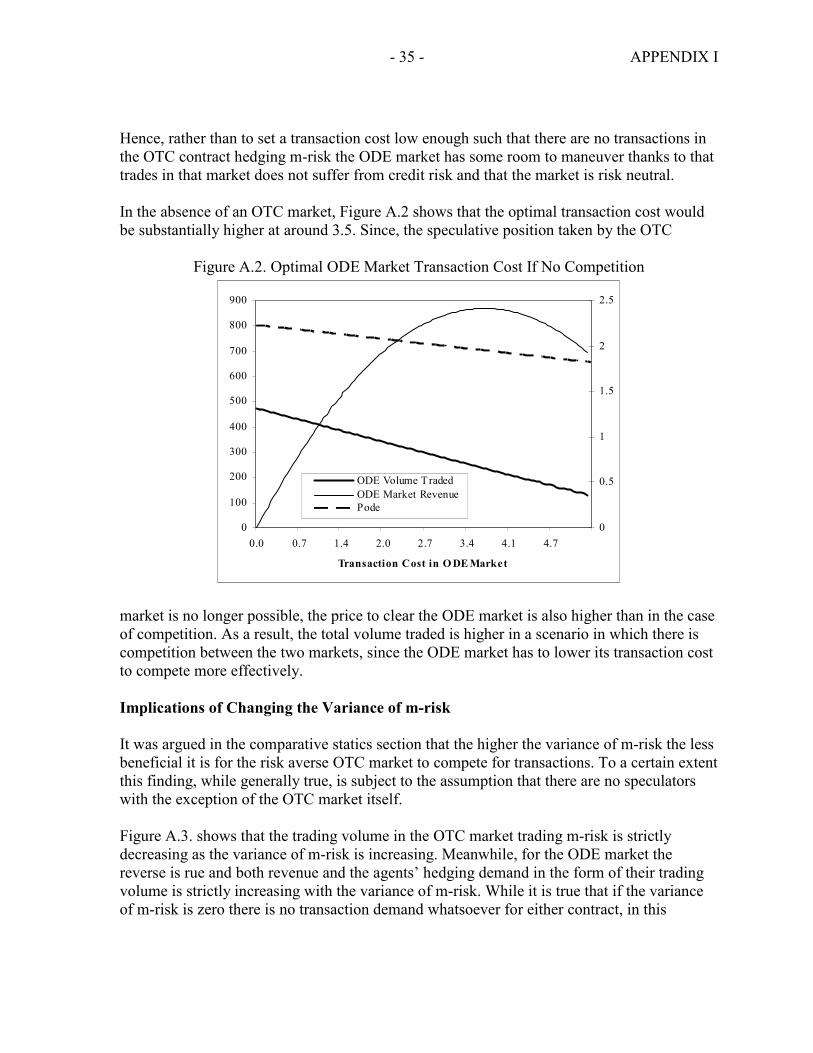
- 35 - APPENDIX I

Hence, rather than to set a transaction cost low enough such that there are no transactions in the OTC contract hedging m-risk the ODE market has some room to maneuver thanks to that trades in that market does not suffer from credit risk and that the market is risk neutral. In the absence of an OTC market, Figure A.2 shows that the optimal transaction cost would be substantially higher at around 3.5. Since, the speculative position taken by the OTC

Figure A.2. Optimal ODE Market Transaction Cost If No Competition

0

100

200

300

400

500

600

700

800

900

0.0 0.7 1.4 2.0 2.7 3.4 4.1 4.7

Transaction Cost in O DE Market

0

0.5

1

1.5

2

2.5

ODE Volume TradedODE Market RevenuePode

market is no longer possible, the price to clear the ODE market is also higher than in the case of competition. As a result, the total volume traded is higher in a scenario in which there is competition between the two markets, since the ODE market has to lower its transaction cost to compete more effectively. Implications of Changing the Variance of m-risk It was argued in the comparative statics section that the higher the variance of m-risk the less beneficial it is for the risk averse OTC market to compete for transactions. To a certain extent this finding, while generally true, is subject to the assumption that there are no speculators with the exception of the OTC market itself. Figure A.3. shows that the trading volume in the OTC market trading m-risk is strictly decreasing as the variance of m-risk is increasing. Meanwhile, for the ODE market the reverse is rue and both revenue and the agents’ hedging demand in the form of their trading volume is strictly increasing with the variance of m-risk. While it is true that if the variance of m-risk is zero there is no transaction demand whatsoever for either contract, in this

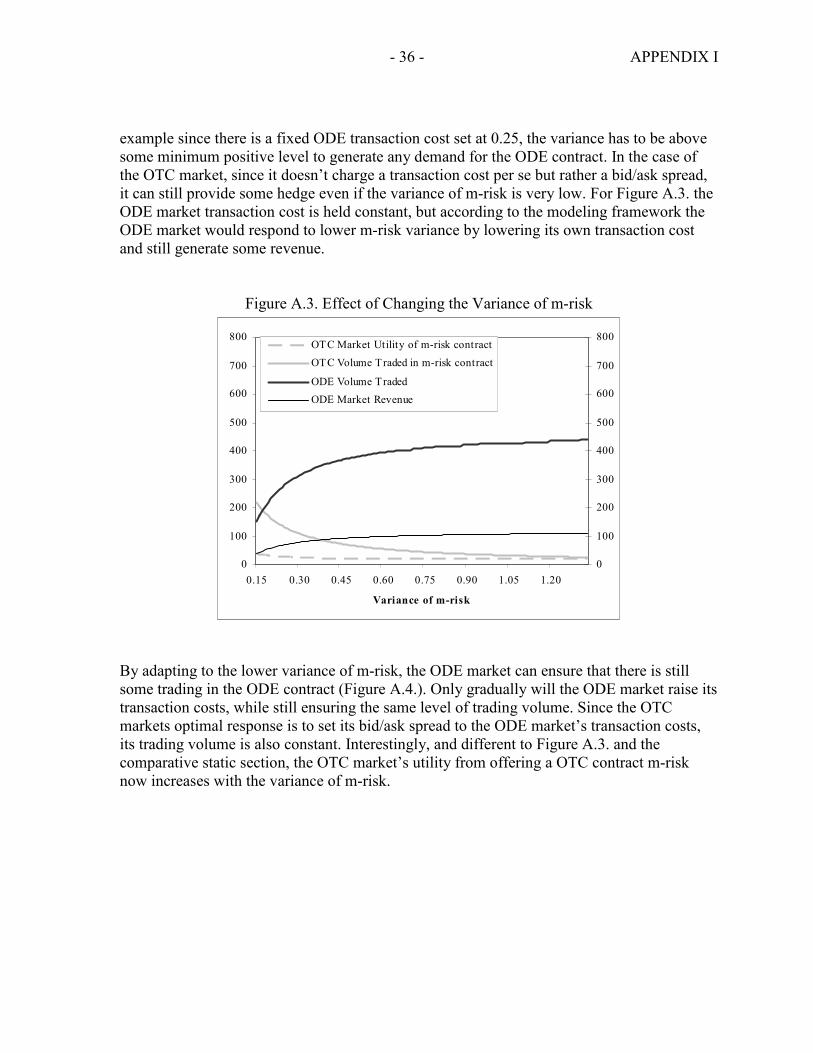
- 36 - APPENDIX I

example since there is a fixed ODE transaction cost set at 0.25, the variance has to be above some minimum positive level to generate any demand for the ODE contract. In the case of the OTC market, since it doesn’t charge a transaction cost per se but rather a bid/ask spread, it can still provide some hedge even if the variance of m-risk is very low. For Figure A.3. the ODE market transaction cost is held constant, but according to the modeling framework the ODE market would respond to lower m-risk variance by lowering its own transaction cost and still generate some revenue.

Figure A.3. Effect of Changing the Variance of m-risk

0

100

200

300

400

500

600

700

800

0.15 0.30 0.45 0.60 0.75 0.90 1.05 1.20

Variance of m-risk

0

100

200

300

400

500

600

700

800OTC Market Utility of m-risk contract

OTC Volume Traded in m-risk contract

ODE Volume TradedODE Market Revenue

By adapting to the lower variance of m-risk, the ODE market can ensure that there is still some trading in the ODE contract (Figure A.4.). Only gradually will the ODE market raise its transaction costs, while still ensuring the same level of trading volume. Since the OTC markets optimal response is to set its bid/ask spread to the ODE market’s transaction costs, its trading volume is also constant. Interestingly, and different to Figure A.3. and the comparative static section, the OTC market’s utility from offering a OTC contract m-risk now increases with the variance of m-risk.

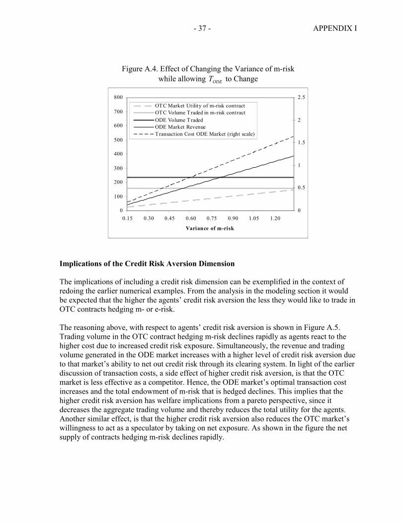
- 37 - APPENDIX I

Figure A.4. Effect of Changing the Variance of m-risk while allowing ODET to Change

0

100

200

300

400

500

600

700

800

0.15 0.30 0.45 0.60 0.75 0.90 1.05 1.20

Variance of m-risk

0

0.5

1

1.5

2

2.5OTC Market Utility of m-risk contractOTC Volume Traded in m-risk contractODE Volume TradedODE Market RevenueTransaction Cost ODE Market (right scale)

Implications of the Credit Risk Aversion Dimension The implications of including a credit risk dimension can be exemplified in the context of redoing the earlier numerical examples. From the analysis in the modeling section it would be expected that the higher the agents’ credit risk aversion the less they would like to trade in OTC contracts hedging m- or e-risk. The reasoning above, with respect to agents’ credit risk aversion is shown in Figure A.5. Trading volume in the OTC contract hedging m-risk declines rapidly as agents react to the higher cost due to increased credit risk exposure. Simultaneously, the revenue and trading volume generated in the ODE market increases with a higher level of credit risk aversion due to that market’s ability to net out credit risk through its clearing system. In light of the earlier discussion of transaction costs, a side effect of higher credit risk aversion, is that the OTC market is less effective as a competitor. Hence, the ODE market’s optimal transaction cost increases and the total endowment of m-risk that is hedged declines. This implies that the higher credit risk aversion has welfare implications from a pareto perspective, since it decreases the aggregate trading volume and thereby reduces the total utility for the agents. Another similar effect, is that the higher credit risk aversion also reduces the OTC market’s willingness to act as a speculator by taking on net exposure. As shown in the figure the net supply of contracts hedging m-risk declines rapidly.

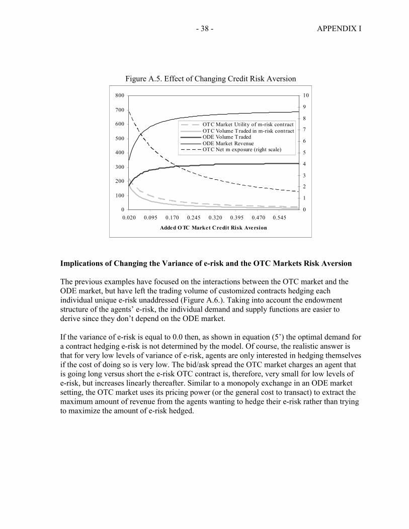
- 38 - APPENDIX I

Figure A.5. Effect of Changing Credit Risk Aversion

0

100

200

300

400

500

600

700

800

0.020 0.095 0.170 0.245 0.320 0.395 0.470 0.545

Added O TC Market Credit Risk Aversion

0

1

2

3

4

5

6

7

8

9

10

OTC Market Utility of m-risk contractOTC Volume Traded in m-risk contractODE Volume TradedODE Market RevenueOTC Net m exposure (right scale)

Implications of Changing the Variance of e-risk and the OTC Markets Risk Aversion The previous examples have focused on the interactions between the OTC market and the ODE market, but have left the trading volume of customized contracts hedging each individual unique e-risk unaddressed (Figure A.6.). Taking into account the endowment structure of the agents’ e-risk, the individual demand and supply functions are easier to derive since they don’t depend on the ODE market. If the variance of e-risk is equal to 0.0 then, as shown in equation (5’) the optimal demand for a contract hedging e-risk is not determined by the model. Of course, the realistic answer is that for very low levels of variance of e-risk, agents are only interested in hedging themselves if the cost of doing so is very low. The bid/ask spread the OTC market charges an agent that is going long versus short the e-risk OTC contract is, therefore, very small for low levels of e-risk, but increases linearly thereafter. Similar to a monopoly exchange in an ODE market setting, the OTC market uses its pricing power (or the general cost to transact) to extract the maximum amount of revenue from the agents wanting to hedge their e-risk rather than trying to maximize the amount of e-risk hedged.

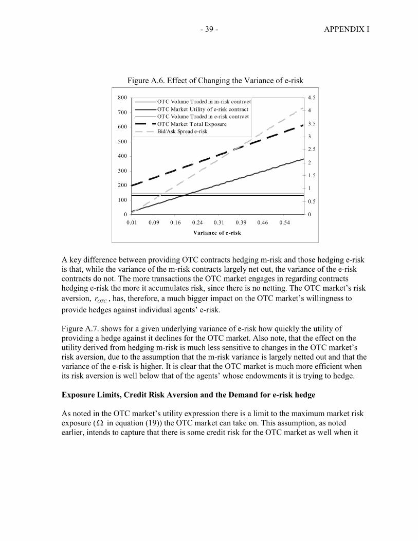
- 39 - APPENDIX I

Figure A.6. Effect of Changing the Variance of e-risk

0

100

200

300

400

500

600

700

800

0.01 0.09 0.16 0.24 0.31 0.39 0.46 0.54

Variance of e -risk

0

0.5

1

1.5

2

2.5

3

3.5

4

4.5OTC Volume Traded in m-risk contractOTC Market Utility of e-risk contractOTC Volume Traded in e-risk contractOTC Market Total ExposureBid/Ask Spread e-risk

A key difference between providing OTC contracts hedging m-risk and those hedging e-risk is that, while the variance of the m-risk contracts largely net out, the variance of the e-risk contracts do not. The more transactions the OTC market engages in regarding contracts hedging e-risk the more it accumulates risk, since there is no netting. The OTC market’s risk aversion, OTCr , has, therefore, a much bigger impact on the OTC market’s willingness to provide hedges against individual agents’ e-risk. Figure A.7. shows for a given underlying variance of e-risk how quickly the utility of providing a hedge against it declines for the OTC market. Also note, that the effect on the utility derived from hedging m-risk is much less sensitive to changes in the OTC market’s risk aversion, due to the assumption that the m-risk variance is largely netted out and that the variance of the e-risk is higher. It is clear that the OTC market is much more efficient when its risk aversion is well below that of the agents’ whose endowments it is trying to hedge. Exposure Limits, Credit Risk Aversion and the Demand for e-risk hedge As noted in the OTC market’s utility expression there is a limit to the maximum market risk exposure (Ω in equation (19)) the OTC market can take on. This assumption, as noted earlier, intends to capture that there is some credit risk for the OTC market as well when it

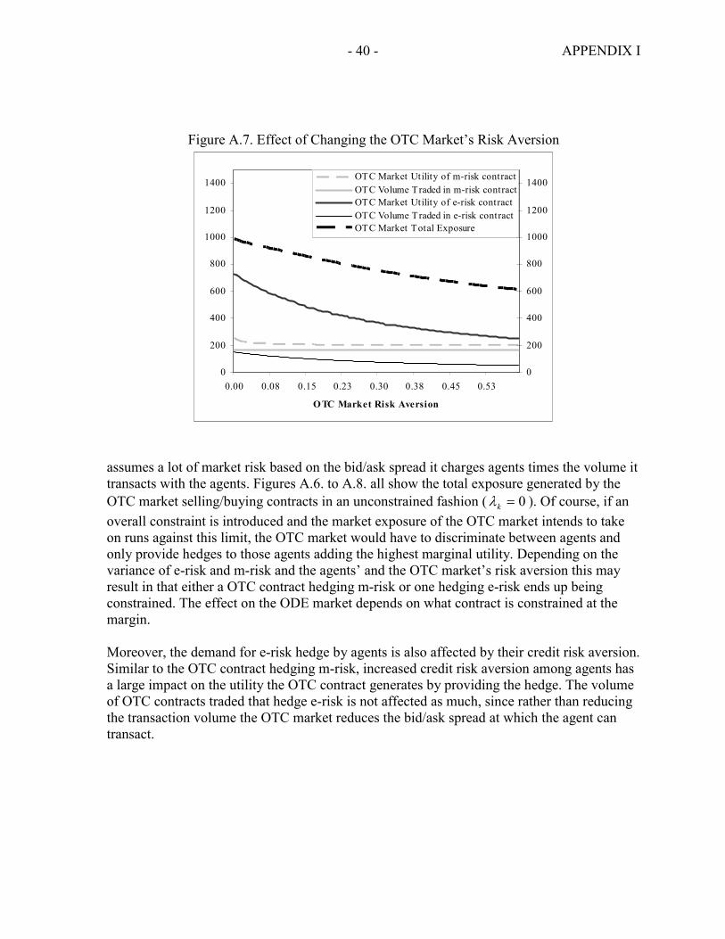
- 40 - APPENDIX I

Figure A.7. Effect of Changing the OTC Market’s Risk Aversion

0

200

400

600

800

1000

1200

1400

0.00 0.08 0.15 0.23 0.30 0.38 0.45 0.53

OTC Market Risk Aversion

0

200

400

600

800

1000

1200

1400OTC Market Utility of m-risk contractOTC Volume Traded in m-risk contractOTC Market Utility of e-risk contractOTC Volume Traded in e-risk contractOTC Market Total Exposure

assumes a lot of market risk based on the bid/ask spread it charges agents times the volume it transacts with the agents. Figures A.6. to A.8. all show the total exposure generated by the OTC market selling/buying contracts in an unconstrained fashion ( 0=kλ ). Of course, if an overall constraint is introduced and the market exposure of the OTC market intends to take on runs against this limit, the OTC market would have to discriminate between agents and only provide hedges to those agents adding the highest marginal utility. Depending on the variance of e-risk and m-risk and the agents’ and the OTC market’s risk aversion this may result in that either a OTC contract hedging m-risk or one hedging e-risk ends up being constrained. The effect on the ODE market depends on what contract is constrained at the margin. Moreover, the demand for e-risk hedge by agents is also affected by their credit risk aversion. Similar to the OTC contract hedging m-risk, increased credit risk aversion among agents has a large impact on the utility the OTC contract generates by providing the hedge. The volume of OTC contracts traded that hedge e-risk is not affected as much, since rather than reducing the transaction volume the OTC market reduces the bid/ask spread at which the agent can transact.

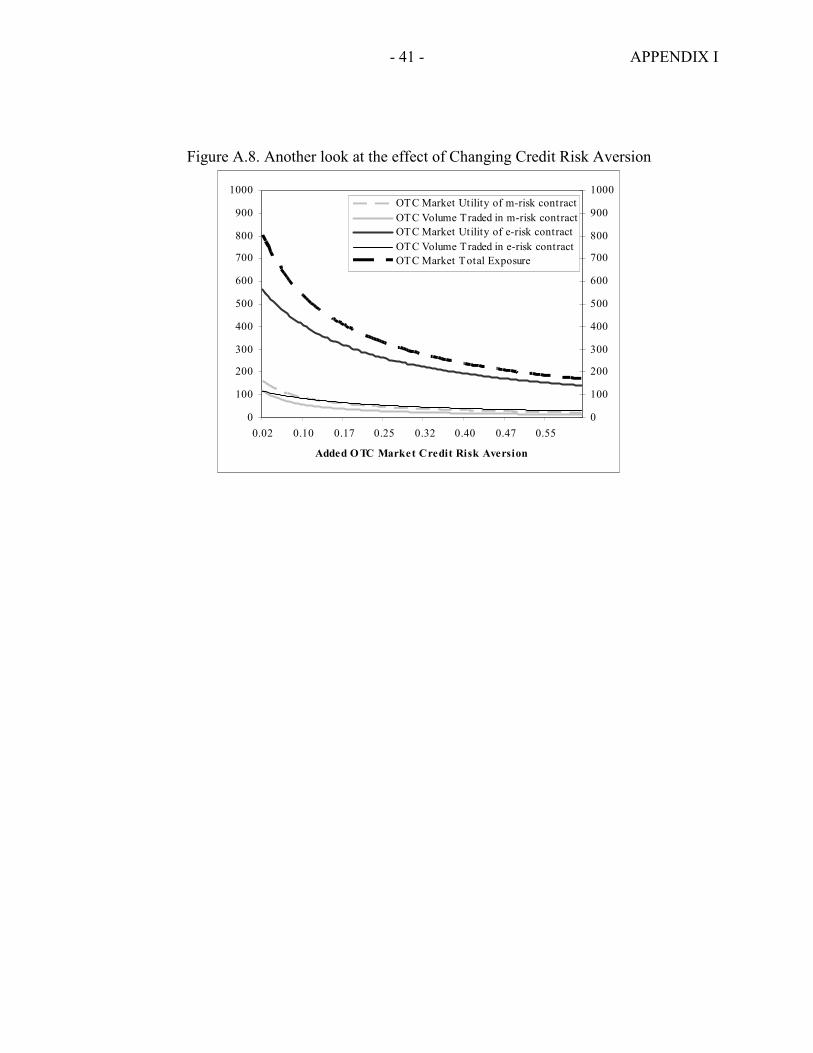
- 41 - APPENDIX I

Figure A.8. Another look at the effect of Changing Credit Risk Aversion

0

100

200

300

400

500

600

700

800

900

1000

0.02 0.10 0.17 0.25 0.32 0.40 0.47 0.55

Added O TC Market Credit Risk Aversion

0

100

200

300

400

500

600

700

800

900

1000OTC Market Utility of m-risk contractOTC Volume Traded in m-risk contractOTC Market Utility of e-risk contractOTC Volume Traded in e-risk contractOTC Market Total Exposure

- 42 - APPENDIX II

REGULATORY AND SUPERVISORY TREATMENT OF OTC VERSUS ODE DERIVATIVES IN THE UNITED STATES

The United States has some of the largest and most innovative OTC issuers, while also being home to some of the world's largest ODE markets. Regulatory agencies, such as the Commodity Futures Trading Commission (CFTC), have generally been cognizant of the potential competitive and systemic threat posed by the OTC market. However, rather than deregulate the ODE markets, much initial discussion dealt with tighter regulation and oversight of OTC markets. The state of regulation globally with respect to OTC swaps and derivatives has been uncertain since the birth of the OTC market.27 In the U.S., laws governing futures transactions were last substantially revised in 1974, establishing the Commodity Exchange Act (CEA) and the CFTC (see ISDA, 1999, and President's Working Group, 1999). These laws were never sufficiently revised to provide the OTC market with regulatory certainty, and the specter of CFTC regulatory oversight remained, threatening the legality of existing swap agreements and OTC derivatives. The illegal aspect originated when the CEA explicitly banned off-exchange "futures" contracts without defining clearly what a "futures" contract was. Therefore, the lack of clarity of the CEA was used by disgruntled investors, after losing substantial amounts of money due to an OTC transaction, to claim that the transaction was illegal to begin with, thereby potentially nullifying the transaction and recovering their losses. A further result of the legislation was that when the American organized derivatives exchange markets, such as the CBOT and the CME, started to seriously feel the competitive pressure from the OTC market, they lobbied the CFTC to take action on OTC derivatives based on the CEA (see Schinasi and others, 2000). OTC market participants' sensitivities were further heightened when the CFTC in 1987 started investigating commodity swaps originated by Chase Manhattan. No enforcement was done but this move and some follow-up efforts forced in response much of the U.S. OTC market off-shore, stifling innovation and increasing costs. Pressure was subsequently brought to bear on the CFTC by the Treasury, the Federal Reserve and industry groups, such as ISDA, to exempt some Swaps from the CEA and CFTC oversight, subject to certain eligibility criteria. The resulting "Swaps Policy Statement" stated "that at this time most swap transactions, although possessing elements of futures or options contracts, are not appropriately regulated as such under the [CEA] and regulations." A swap was hence considered safe from the CEA if certain criteria were satisfied. While a significant percentage of OTC swaps satisfied these criteria at the time, new OTC derivative innovations again caused an increase in regulatory uncertainty. Regulators (see President's Working Group, 1999) after being increasingly concerned about the systemic risk posed by OTC derivatives, became aware that the list of criteria did not cover all relevant OTC derivatives and that these criteria also directly discouraged the use of clearing systems in part to ameliorate the systemic risk concerns. After another round of court cases, which tried to define the

27 A brief review is given below, but for a detailed discussion see ISDA (1999) and President's Working Group (1999).

- 43 - APPENDIX II

difference between a futures contract and a forward contract the U.S. Congress finally decided to act in 1992, and amended the CEA with the adoption of the Futures Trading Practices Act. The Act provided increased legal certainty by allowing and expecting the CFTC to exempt OTC contracts from CEA regulation, especially the exchange-trading requirement, without first determining whether the contract was subject to the CEA to begin with. This was a major step forward for the OTC market and the CFTC adopted early 1993 a broad exemption for swap agreements and other OTC derivatives, as long as they were conducted by "eligible swap participants." 28 29 Furthermore, to be exempted, the OTC contract had to be customized and not traded on or through a "multilateral transaction execution facility" (MTEF). A conscious omission was not to give the CFTC the power to exempt OTC derivatives based on individual securities.30 In addition, the outstanding issue of whether swap contracts and other OTC derivatives were actually subject to the CEA was never settled. In 1998, the CFTC issued a comment letter on a regulatory action and a concept release (see CFTC (1998)), which were widely interpreted as a move to increase regulation and CFTC supervision of the OTC market. This caused some concern because it would almost by necessity increase the transaction costs and perhaps cause the OTC market to move again offshore. Market participants, especially those trading in non-exempted securities, such as equity swaps, credit swaps and emerging market debt swaps, reacted negatively and the Treasury, the Federal Reserve, and industry groups pushed Congress to impose a stay on the CFTC.31 It was clear that the OTC market had developed fast, and old definitions and exemptions were no longer adequate, hampering more efficient developments and innovations. Furthermore, ODE markets were increasingly pressing the CFTC for their own regulatory relief and a level playing field. In the aftermath, Congress gave the key regulatory agencies, through the so called President's Working Group on Financial Markets, the task to present reforms that would address the OTC markets' key concerns and take steps to reduce systemic risk. The regulatory agencies' findings led quickly to the passing of the Commodity Futures Modernization Act (CFMA) by end-2000. The main changes implied by the CFMA are:32 28 Swaps and OTC derivatives were, however, not exempted from anti-fraud and anti-manipulation regulation. 29 For a definition see ISDA (1999), but basically "eligible swap participants" are financial corporations and high net worth individuals, i.e., not the broad public. 30 Other than exempt securities, such as government bonds. The agreement that restructured the scope of the CEA and its relationship to the Securities and Exchange Commission was called the Shad-Johnson Accord. 31 Securities that were not exempted and fell on the borderline in the Shad-Johnson Accord. 32 See page 2 of the report for a summary.

- 44 - APPENDIX II

• Various clarifications of the legal certainty of OTC transactions, noting that all existing ones are legal, and new ones will be exempt from the CEA to a much larger extent.

• The exclusion from the CEA for electronic trading systems, the MTEF criteria, as long as participants are sophisticated enough. This exemption is open, as well, for existing organized derivative exchange markets, as well as for OTC markets, opening up for professional actors’ markets in futures trading.

• Eliminate impediments in current law for the clearing of OTC transactions, as long as the clearing organization is sufficiently supervised.

• Single-stock futures may be allowed, which was seen as a boon for futures exchanges.

The objective of the new law is to make sure that regulatory certainty leads to a reduction in transaction costs in many OTC market segments, that special purpose vehicle structures be eliminated, or substantially simplified with a drop in legal cost, and off-shore transactions can be brought back on-shore. Furthermore, increased certainty will allow OTC markets to develop instruments that previously were not offered as the legal basis was not clear. In relation to the model developed later in this paper, such a regulatory reform could lead to less competition between the markets, as OTC markets are freer to specialize in their comparative advantage. Hence, as would be predicted, most ODE markets largely welcomed the initial report (see Chicago Board of Trade, Chicago Mercantile Exchange, New York Mercantile Exchange press release, 1999) and eventual passing of the CFMA law. However, ODE markets remained disappointed since the CFMA, in their view, leaves the non-level regulatory and supervisory playing field broadly intact. In fact, ODE markets have continued to support regulatory efforts to increase the disclosure requirements for OTC participants, and proposals to expand regulation of the OTC markets were once again recently proposed in the U.S. Senate.33 Again, from the competition viewpoint of the model developed in this paper, ODE markets could gain from the CFMA and should support further deregulation of the OTC market. Moreover, setting up clearing facilities or introducing OTC like instruments on their own exchanges could be a successful strategy to enhance in turn the OTC market's capability to take on highly customized/idiosyncratic risk.34 Leveling the playing field by deregulating the ODE markets remains an outstanding issue, where new initiatives could decrease transaction costs and subsequently increase overall volume traded. However, the ODE markets’ role in 33 In September 2002, U.S. Senators Harkin and Lugar proposed expanded regulation of the OTC markets. The federal regulatory and supervisory agencies quickly issued a strong statement against such initiatives. 34 CBOT recent decision to launch an interest rate swap contract is one example of a likely successful strategy.

- 45 - APPENDIX II

price discovery and the federal agencies’ interest in protecting end-users of ODE derivatives make any deregulatory initiatives hard to enact. Broadly speaking, the CFMA codified the limited regulatory and supervisory oversight of OTC markets, while ODE markets continued to be regulated and supervised by the CFTC. However, the CFTC takes a largely sanguine view on the competitive pressures facing its ODE markets from others abroad as well as from OTC markets. In a recent report (CFTC (1999)), the agency noted that the global competitiveness of U.S. futures markets remained high and not a real source of concern, a view clearly not widely shared outside the regulatory and supervisory communities.

- 46 -

REFERENCES Allen, F., and D. Gale, 1994, Financial Innovation and Risk Sharing, (Cambridge,

Massachusetts: MIT Press). Arbor, P., 1997, Testimony of Patrick H. Arbor before the Risk Management and Specialty

Crops Subcommittee of the House Agriculture Committee, Board of Trade of the City of Chicago (April 15).

Bank for International Settlements, 1997-2002, various issues, International Banking and

Financial Market Developments, (Basel: Bank for International Settlements). ———, 1998, OTC Derivatives: Settlement Procedures and Counterparty Risk Management, (Basel: Bank for International Settlements). ———, 1999, Central Bank Survey of Foreign Exchange and Derivatives Market Activity,

(Basel: Bank for International Settlements). ———,2002, Triennial Central Bank Survey: Foreign Exchange and Derivative Market

Activity in 2001, (Basel: Bank for International Settlements). Brennan, D., 1999, Testimony of David P. Brennan, Chairman, Board of Trade of the City of

Chicago (September 23). Chicago Board of Trade, Chicago Mercantile Exchange, New York Mercantile Exchange,

1999, CME, CBOT, NYMEX Respond to Report of President's Working Group on Financial Markets, (New York).

Commodities Futures Trading Commission, 1998, Concept Release on Over-the-Counter

Derivatives, (Washington: Commodity Futures Trading Commission). ———, 1999, The Global Competitiveness of U.S. Futures Markets Revisited, Division of

Economic Analysis, (Washington: Commodity Futures Trading Commission). Cuny, C., 1993, “The Role of Liquidity in Futures Market Innovations,” Review of Financial

Studies, Vol. 6, pp. 57–78. Duffie, D., and M. Jackson, 1989, “Optimal Innovation of Futures Contracts,” Review of

Financial Studies, Vol. 2, pp. 275–96. ———, 1992, “The Nature of Incomplete Security Markets,” in ed. by Jean-Jacques Laffont,

Advances in Economic Theory: Sixth World Congress, Vol. 2, (Cambridge University Press), pp. 214–62.

———, and R. Rahi, 1995, “Financial Market Innovation and Security Design,” Journal of

Economic Theory, Vol. 65, pp. 1–42.

- 47 -

———, and K. Singleton, 2003, “Credit Risk: Pricing, Measurement, and Management,”

(Princeton University Press). Group of Thirty, 1993, “Special Report on Global Derivatives,” Washington. International Swaps Dealer Association, 1999, Statement Submitted to the Subcommittee on

Risk Management and Specialty Crops, (May 17). Kroszner, R., 1999, “Can the Financial Markets Privately Regulate Risk?,” Journal of

Money, Credit, and Banking, Vol. 31, No. 3, pp. 596–618. Melamed, L., 2000, “Futures Markets in an E-commerce World”, Speech delivered at

Canadian Annual Derivatives Conference (October). United States, Office of the Comptroller of the Currency, 1999, OCC Bank Derivatives

Report, Second Quarter (Washington). ———, 2002, OCC Bank Derivatives Report, Second Quarter (Washington). United States, President's Working Group on Financial Markets, 1999, Over-the-Counter

Derivatives Markets and the Commodity Exchange Act (Washington). United States, Department of the Treasury, Board of Governors of the Federal Reserve

System, Securities and Exchange Commission, and Commodity Futures Trading Commission, 2002, Response to Letter of Senators Crapo and Miller (September 18).

Rahi, R., and J. Zigrand, 2004, “Strategic Financial Innovation in Segmented Markets,”

Working Paper, “Centre for Economic Policy Research, No. 4176.” Rainer, W., 1999, Remarks of William J. Rainer Chairman delivered at the 22nd Annual

Chicago-Kent College of Law, Commodity Futures Trading Commission (October 28).

Santos, T., and J. Sheinkman, 2001, “Competition Among Exchanges”, Quarterly Journal of

Economics, August. Schinasi, G., R. Craig, B. Drees, and C. Kramer, 2000, “Modern Banking and OTC

Derivatives Markets”, IMF Occasional Paper No. 203 (Washington: International Monetary Fund).

Tashjian, J. and M. Weissman, 1995, “Advantages of Competing with Yourself: Why an

Exchange Might Design Futures Contracts with Correlated Payoffs,” Journal of Financial Intermediation, Vol. 4, pp. 133–57.