U.S. Department of the InteriorU.S. Geological Survey

Depth Calibration of the Experimental Advanced Airborne Research Lidar, EAARL-BBy C. Wayne Wright, Christine J. Kranenburg, Rodolfo J. Troche, Richard W. Mitchell, and David B. Nagle

Open-File Report 2016–1048

ii

U.S. Department of the InteriorSALLY JEWELL, Secretary

U.S. Geological SurveySuzette M. Kimball, Director

U.S. Geological Survey, Reston, Virginia: 2016

For more information on the USGS—the Federal source for science about the Earth, its natural and living resources, natural hazards, and the environment—visit http://www.usgs.gov or call 1–888–ASK–USGS.

For an overview of USGS information products, including maps, imagery, and publications, visit http://store.usgs.gov/.

Any use of trade, firm, or product names is for descriptive purposes only and does not imply endorsement by the U.S. Government.

Although this information product, for the most part, is in the public domain, it also may contain copyrighted materials as noted in the text. Permission to reproduce copyrighted items must be secured from the copyright owner.

Suggested citation: Wright, C.W., Kranenburg, C.J., Troche, R.J., Mitchell, R.W., and, Nagle, D.B., 2016, Depth calibration of the experimen-tal advanced airborne research lidar, EAARL-B: U.S. Geological Survey Open-File Report 2016–1048, 23 p., http://dx.doi.org/10.3133/ofr20161048.

ISSN 2331-1258 (online)

iii

ContentsAcknowledgments ...........................................................................................................................................................................................vi1. Introduction .................................................................................................................................................................................................. 12. Background ................................................................................................................................................................................................. 2

2.1 The EAARL-B Sensor ........................................................................................................................................................................... 22.2 Raster versus Conical or Circular Scanning ......................................................................................................................................... 42.3 Position and Orientation-Induced Errors ............................................................................................................................................... 52.4 The IHO Standard ................................................................................................................................................................................. 52.5 Reference Datasets .............................................................................................................................................................................. 6

2.5.1 The JALBTCX Primary Reference Dataset ................................................................................................................................... 62.5.2 Supplemental Reference Data....................................................................................................................................................... 7

2.6 The Central Questions .......................................................................................................................................................................... 73. Methods ....................................................................................................................................................................................................... 8

3.1 Subaerial Calibration ............................................................................................................................................................................. 83.2 Shallow-Water Calibration of the Deep Channel ................................................................................................................................... 83.3 Calibration Mission Flights .................................................................................................................................................................... 93.4 Selection of Calibration Regions ......................................................................................................................................................... 103.5 Data Processing, Filtering, and Editing ............................................................................................................................................... 10

3.5.1 Processing Software .................................................................................................................................................................... 103.5.2 Random Consensus Filtering ...................................................................................................................................................... 123.5.3 Manual Editing ............................................................................................................................................................................. 133.5.4 Point-to-Point Comparison and Difference .................................................................................................................................. 13

3.6 Derivation of the Calibration Constants ............................................................................................................................................... 144. Results and Discussion ............................................................................................................................................................................. 15

4.1 Analysis of Raw Mean Differences ...................................................................................................................................................... 154.2 Comparison of Uncalibrated Depths with Calibrated Depths .............................................................................................................. 164.3 Comparison of Calibrated Results with IHO Standards ...................................................................................................................... 164.4 Comparison of Deep-channel to Shallow-channel Depth Measurements ........................................................................................... 16

5. Conclusions ............................................................................................................................................................................................... 196. References Cited ....................................................................................................................................................................................... 207. Appendix 1 ................................................................................................................................................................................................. 21

Processing Parameters, South Florida Testing Facility (SFTF) Calibration Site ....................................................................................... 21

iv

Figures 1. Overview map showing location of the South Florida Testing Facility ............................................................................................ 2 2. Footprint of the EAARL-B receiver ................................................................................................................................................. 3 3. Mean error of runway calibration flights from 2012 to 2014 ............................................................................................................ 8 4. Density estimates and statistics of vertical error before and after channel alignment .................................................................... 9 5. Selected depth regimes, which are relatively flat, level, and free of sand, seagrass, and small-scale bottom structure ...............11 6. Difference map between EAARL-B and JALBTCX reference data .............................................................................................. 12 7. Components of the shallow and deep water bathymetry processing algorithms .......................................................................... 13 8. Scatterplot of raw EAARL-B depths to reference dataset mean differences ................................................................................ 14 9. Kernel density estimates of vertical error for select depth regions ............................................................................................... 17 10. Mean differences of uncalibrated and calibrated EAARL-B data .................................................................................................. 18 11. Mean differences and 95 percent accuracy of calibrated EAARL-B data ..................................................................................... 18 12. Comparison of deep-channel to shallow-channel depth measurements ...................................................................................... 19

Tables 1. International Hydrographic Organization (IHO) minimum standards for hydrographic surveys. ..................................................... 6 2. Maximum allowableTotal Vertical Uncertainty (TVU) values for various depths (meters). .............................................................. 6 3. Statistics of pre-calibration vertical error, per region, at the SFTF site. ........................................................................................ 15 1–1. ALPS bathymetry-processing parameters used for data in this publication. ................................................................................ 21 1–2. EAARL-B operations-configuration parameters used for data in this publication. ........................................................................ 22

v

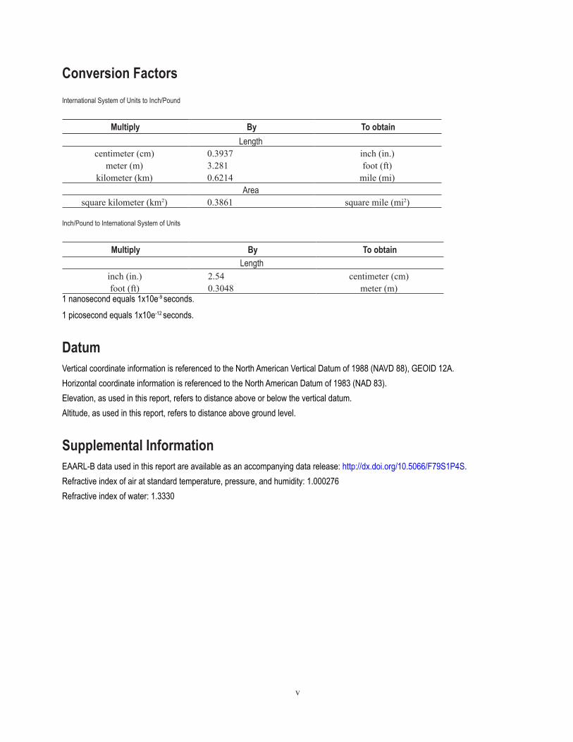
Conversion FactorsInternational System of Units to Inch/Pound

Multiply By To obtainLength

centimeter (cm) 0.3937 inch (in.)meter (m) 3.281 foot (ft)

kilometer (km) 0.6214 mile (mi)Area

square kilometer (km2) 0.3861 square mile (mi2)

Inch/Pound to International System of Units

Multiply By To obtainLength

inch (in.) 2.54 centimeter (cm) foot (ft) 0.3048 meter (m)

1 nanosecond equals 1x10e-9 seconds.1 picosecond equals 1x10e-12 seconds.

DatumVertical coordinate information is referenced to the North American Vertical Datum of 1988 (NAVD 88), GEOID 12A.Horizontal coordinate information is referenced to the North American Datum of 1983 (NAD 83).Elevation, as used in this report, refers to distance above or below the vertical datum.Altitude, as used in this report, refers to distance above ground level.

Supplemental InformationEAARL-B data used in this report are available as an accompanying data release: http://dx.doi.org/10.5066/F79S1P4S.Refractive index of air at standard temperature, pressure, and humidity: 1.000276Refractive index of water: 1.3330

vi

AbbreviationsALPS Airborne Lidar Processing SystemANSI American National Standards Institutecm centimeterCORS Continuously Operating Reference StationCZMIL Coastal Zone Mapping and Imaging LidarEAARL Experimental Advanced Airborne Research Lidar, original versionEAARL-B Experimental Advanced Airborne Research Lidar, Version “B”GPS Global Positioning SystemIHO International Hydrographic OrganizationITRF International Terrestrial Reference FrameJALBTCX Joint Airborne Lidar Bathymetry Technical Center of ExcellenceLAS Laser data file formatLaser Light Amplification by Stimulated Emission of RadiationLidar Light Detection and Rangingm meterNASA National Aeronautics and Space AdministrationNGS National Geodetic SurveyNOAA National Oceanic and Atmospheric AdministrationPMT Photomultiplier TubeRCF Random Consensus FilterRMSE Root Mean Square ErrorSFTF South Florida Testing FacilitySHOALS Scanning Hydrographic Operational Airborne Lidar SystemSonar Sound Navigation and RangingTTS Transit Time SpreadTVU Total Vertical UncertaintyUSACE U.S. Army Corps of EngineersUSGS U.S. Geological SurveyWGS-84 World Geodetic System (1984)

AcknowledgmentsThe U.S. Geological Survey Coastal and Marine Geology Program funded the survey mission described herein and the development of this paper. The authors gratefully acknowledge Dr. Jennifer Wozencraft, Christopher Macon, and Nick Johnson of the U.S. Army Corps of Engineers for sharing the primary reference dataset without which this effort would not have been possible. We also thank Karen Morgan of the U.S. Geological Survey for her invaluable assistance as sensor operator for the duration of this survey.

1

Depth Calibration of the Experimental Advanced Airborne Research Lidar, EAARL-BBy C. Wayne Wright, Christine J. Kranenburg, Rodolfo J. Troche, Richard W. Mitchell, and David B. Nagle

1. IntroductionThe original National Aeronautics and Space Administration (NASA) Experimental Advanced

Airborne Research Lidar (EAARL) was extensively modified to increase the spatial sampling density and to improve performance in water ranging from 3 to 44 meters (m). The new (EAARL-B) sensor fea-tures a higher spatial density that was achieved by optically splitting each laser pulse into three pulses spatially separated by 1.6 m along the flight track and 2.0 m across the flight track, on the water surface, when flown at a nominal altitude of 300 m (984 feet). The sample spacing can be optionally increased to 1.0 m across the flight track. Improved depth capability was achieved by increasing the total peak laser power by a factor of 10 and by designing a new “deep-water” receiver, which is optimized to exclu-sively receive refracted and scattered light from deeper water (15–44 m).

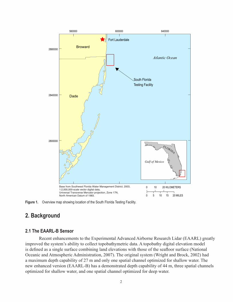
Two different clear-water flight missions were conducted over the U.S. Navy’s South Florida Testing Facility (SFTF) to determine the EAARL-B calibration coefficients. The SFTF is an established lidar calibration range located in the coastal waters southeast of Fort Lauderdale, Florida (fig. 1). We used 23 selected polygons at 23 distinct depths to compare a reference dataset from this site to deter-mine EAARL-B calibration constants over the depth range of 6.5 to 34 m.

We also conducted a near-simultaneous single-beam jet-ski-based sonar survey of selected transects ranging from 1 to 33 m depth in the same area. The near-concurrent jet ski data were used to evaluate the EAARL-B performance over the depth range from 0.9 to 10 m. The more timely jet ski data were necessary because the primary reference dataset was 9 years old, and areas shallower than 6.5 m are dominated by shifting sand. We determined the jet ski data were not useful as a calibration reference in water deeper than 10 m due to large uncertainty in the vertical measurement introduced by the lack of any sensor orientation data, that is, for pitch, roll, and heading to correct the measured slant range to a vertical measurement.

The resulting calibrated EAARL-B data were then analyzed and compared with the original reference dataset, the jet-ski-based dataset from the same Fort Lauderdale site, as well as the depth-accuracy requirements of the International Hydrographic Organization (IHO). We do not claim to meet all of the IHO requirements and standards. The IHO minimum depth-accuracy requirements were used as a reference only and we do not address the other IHO requirements such as “Full Seafloor Search” (International Hydrographic Bureau, 2008). Our results show good agreement between the calibrated EAARL-B data and all reference datasets, with results that are within the 95 percent depth accuracy of the IHO Order 1 (a and b) depth-accuracy requirements.

2

2. Background

2.1 The EAARL-B SensorRecent enhancements to the Experimental Advanced Airborne Research Lidar (EAARL) greatly

improved the system’s ability to collect topobathymetric data. A topobathy digital elevation model is defined as a single surface combining land elevations with those of the seafloor surface (National Oceanic and Atmospheric Administration, 2007). The original system (Wright and Brock, 2002) had a maximum depth capability of 27 m and only one spatial channel optimized for shallow water. The new enhanced version (EAARL-B) has a demonstrated depth capability of 44 m, three spatial channels optimized for shallow water, and one spatial channel optimized for deep water.

0 10 20 KILOMETERS

0 5 10 15 20 MILES

Dade

Broward

560000 600000 640000

2800000

2840000

2880000

Atlantic Ocean

South FloridaTesting Facility

Fort Lauderdale

Base from Southwest Florida Water Management District, 2003, 1:2,000,000-scale vector digital data, Universal Transverse Mercator projection, Zone 17N, North American Datum of 1983.

Gulf of Mexico

FLORIDA

Figure 1. Overview map showing location of the South Florida Testing Facility.

3

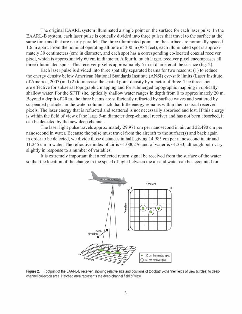
The original EAARL system illuminated a single point on the surface for each laser pulse. In the EAARL-B system, each laser pulse is optically divided into three pulses that travel to the surface at the same time and that are nearly parallel. The three illuminated points on the surface are nominally spaced 1.6 m apart. From the nominal operating altitude of 300 m (984 feet), each illuminated spot is approxi-mately 30 centimeters (cm) in diameter, and each spot has a corresponding co-located coaxial receiver pixel, which is approximately 60 cm in diameter. A fourth, much larger, receiver pixel encompasses all three illuminated spots. This receiver pixel is approximately 5 m in diameter at the surface (fig. 2).

Each laser pulse is divided into three spatially separated beams for two reasons: (1) to reduce the energy density below American National Standards Institute (ANSI) eye-safe limits (Laser Institute of America, 2007) and (2) to increase the spatial point density by a factor of three. The three spots are effective for subaerial topographic mapping and for submerged topographic mapping in optically shallow water. For the SFTF site, optically shallow water ranges in depth from 0 to approximately 20 m. Beyond a depth of 20 m, the three beams are sufficiently refracted by surface waves and scattered by suspended particles in the water column such that little energy remains within their coaxial receiver pixels. The laser energy that is refracted and scattered is not necessarily absorbed and lost. If this energy is within the field of view of the large 5-m diameter deep-channel receiver and has not been absorbed, it can be detected by the new deep channel.

The laser light pulse travels approximately 29.971 cm per nanosecond in air, and 22.490 cm per nanosecond in water. Because the pulse must travel from the aircraft to the surface(s) and back again in order to be detected, we divide those distances in half, giving 14.985 cm per nanosecond in air and 11.245 cm in water. The refractive index of air is ~1.000276 and of water is ~1.333, although both vary slightly in response to a number of variables.

It is extremely important that a reflected return signal be received from the surface of the water so that the location of the change in the speed of light between the air and water can be accounted for.

Figure 2. Footprint of the EAARL-B receiver, showing relative size and positions of topobathy-channel fields of view (circles) to deep-channel collection area. Hatched area represents the deep-channel field of view.

60 cm receiver pixel30 cm illuminated spot

5 meters

5 mete

rs

5 meters

scandirection

4

Two distinct mechanisms can produce a signal from the surface region. The first is the reflection from the discontinuity in dielectric between air and water, and the second is largely from suspended particu-late material at or near the surface. The difference in how these two mechanisms reflect light is critically important. The first mechanism produces a highly specular reflection—the reflected fraction of the incident light is reflected at the same but opposite angle with respect to the surface normal. This surface reflection varies strongly as a function of lidar scan angle and surface sea state. The second mechanism is non-specular, and its strength depends on suspended particulate matter in the water column. Although particulates help generate a good signal at or near the surface, they also limit the depth measurement capability of the lidar. Additionally, suspended sediment tends to spread the returned laser pulse, making it difficult to use for determining exactly where the surface is (Guenther and others, 1994).

Each channel of the EAARL-B uses a photomultiplier tube (PMT) to measure the incoming reflected laser light. A PMT is an extremely fast photodetector. The transit time of a PMT is the time delay between the arrival of a light pulse at the PMT and appearance of the amplified electrical output pulse (Hamamatsu Photonics K.K., 2007). The three topobathy channels use identical PMTs with a photoelectron transit time of 5,400 picoseconds and a transit time spread (TTS) of 230 picoseconds, which contribute to the error budget an uncertainty in slant-range measurement of 3.4 cm in air and 2.5 cm in water, whereas the deep channel uses a different, more sensitive and higher gain PMT with a photoelectron transit time of 2,700 picoseconds and an electron TTS of 200 picoseconds, which cor-responds to 2.95 cm in air and 2.2 cm in water. These transit time spreads establish the absolute lower limit of ranging uncertainty of the EAARL-B.

2.2 Raster versus Conical or Circular ScanningThe EAARL-B uses a raster scanner that is more typical of topographic lidars. Most bathy-

metric lidars use a conical, circular, or semi-circular scan pattern for two primary reasons: (1) it yields a relatively constant and substantial off-nadir angle of incidence to the water surface, and (2) it helps reduce the dynamic range of the water-surface Fresnel reflection, which in turn reduces the overload performance requirements of the receiver channel(s). One important disadvantage of conical and cir-cular scanning is the constant high geometric pulse spreading it causes. This effect occurs because most bathymetric lidars illuminate relatively large (~2 m) spots on the surface of the water which increases the geometric surface-regime pulse stretching and decreases the accuracy of the surface-return elevation measurement. It is currently impractical or even impossible to know from what portion of the stretched, illuminated spot the reflected energy is returned.

The EAARL-B raster scan is tilted a few degrees forward to avoid nadir surface Fresnel reflec-tions. The system must demonstrate that it is capable of accurate submerged-topography measurement over a wide range of laser angles of incidences and in the presence of strong surface-return reflec-tions because it scans over a much larger range of scan angles than circular or conical scanners. One advantage of the raster scan is a more uniform distribution of surface points at a given laser pulse rate. Another advantage is that a significant number of points are collected near nadir where pitch, roll, and yaw error contributions are minimal. Conical and circular scanners operate with the maximum pitch, roll, and yaw error contributions at all times. The EAARL-B varies its pulse rate as a function of the scan angle to enhance surface-sample distribution.

5

2.3 Position and Orientation-Induced ErrorsA substantial portion of the uncertainty budget for the EAARL-B comes from the uncertainty

of the Global Positioning System (GPS)-determined position of the aircraft. Major contributors to GPS position errors are (1) satellite: geometry, visibility, health, and number of satellites, (2) baseline dis-tance between the aircraft and the reference base station, and (3) weather conditions, carrier cycle slips, and so forth (Grewal and others, 2013).

Another important source of uncertainty and error is the accurate determination of the aircraft orientation in terms of pitch, roll, and heading. The orientation determination is closely linked to the position uncertainty because the position values are used to update the Kalman filters in the orientation solutions (Ford and Hamilton, 2003; Grewal and others, 2013).

The position and orientation uncertainties add to the lidar range-measurement uncertainty and the scan-angle uncertainty. For bathymetric measurement, additional uncertainty comes from inac-curacies in detecting the water surface (Guenther and others, 1994; Guenther and others, 1996). Rather than examining the component parts of the error budget, we will examine the total system bottom-line measured performance.

2.4 The IHO StandardThe EAARL-B was not designed with the intent of meeting the IHO S-44-5E Minimum Stan-

dards for Hydrographic Surveys (International Hydrographic Bureau, 2008). However, the depth-mea-surement uncertainty criteria for IHO Special Order, and Order 1 (a and b) surveys provide a convenient means for assessing and describing the results of the EAARL-B performance evaluation.

The IHO Special Order and Order 1 standards also include requirements for bottom-feature detection and full seafloor search, and all have horizontal-accuracy requirements. However, this study makes no claim to meet these requirements, and no work was done on feature detection, full seafloor search, or analysis of the results for horizontal accuracy. We are exclusively using the vertical depth requirements of the IHO Special Order, and Order 1 as convenient references for acceptable depth-accuracy performance. The IHO defines Total Vertical Uncertainty (TVU) as the vertical component of the total propagated uncertainty. Total propagated uncertainty includes both random and systematic measurement uncertainties as well as those introduced from derived or calculated parameters. The maximum allowable TVU at the 95 percent confidence level is computed as follows:

(1)

where

a represents that portion of the uncertainty that does not vary with depth;

b is a coefficient which represents the portion of the uncertainty that varies as a function of depth; and

d is the depth, in meters; therefore,

bd is the portion of the uncertainty that varies with depth.

6

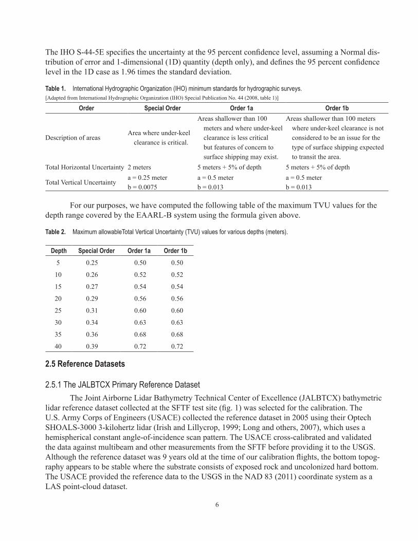
The IHO S-44-5E specifies the uncertainty at the 95 percent confidence level, assuming a Normal dis-tribution of error and 1-dimensional (1D) quantity (depth only), and defines the 95 percent confidence level in the 1D case as 1.96 times the standard deviation.

Table 1. International Hydrographic Organization (IHO) minimum standards for hydrographic surveys.[Adapted from International Hydrographic Organization (IHO) Special Publication No. 44 (2008, table 1)]

Order Special Order Order 1a Order 1b

Description of areasArea where under-keel

clearance is critical.

Areas shallower than 100 meters and where under-keel clearance is less critical but features of concern to surface shipping may exist.

Areas shallower than 100 meters where under-keel clearance is not considered to be an issue for the type of surface shipping expected to transit the area.

Total Horizontal Uncertainty 2 meters 5 meters + 5% of depth 5 meters + 5% of depth

Total Vertical Uncertaintya = 0.25 meterb = 0.0075

a = 0.5 meterb = 0.013

a = 0.5 meterb = 0.013

For our purposes, we have computed the following table of the maximum TVU values for the depth range covered by the EAARL-B system using the formula given above.

Table 2. Maximum allowableTotal Vertical Uncertainty (TVU) values for various depths (meters).

Depth Special Order Order 1a Order 1b5 0.25 0.50 0.50

10 0.26 0.52 0.52

15 0.27 0.54 0.54

20 0.29 0.56 0.56

25 0.31 0.60 0.60

30 0.34 0.63 0.63

35 0.36 0.68 0.68

40 0.39 0.72 0.72

2.5 Reference Datasets

2.5.1 The JALBTCX Primary Reference DatasetThe Joint Airborne Lidar Bathymetry Technical Center of Excellence (JALBTCX) bathymetric

lidar reference dataset collected at the SFTF test site (fig. 1) was selected for the calibration. The U.S. Army Corps of Engineers (USACE) collected the reference dataset in 2005 using their Optech SHOALS-3000 3-kilohertz lidar (Irish and Lillycrop, 1999; Long and others, 2007), which uses a hemispherical constant angle-of-incidence scan pattern. The USACE cross-calibrated and validated the data against multibeam and other measurements from the SFTF before providing it to the USGS. Although the reference dataset was 9 years old at the time of our calibration flights, the bottom topog-raphy appears to be stable where the substrate consists of exposed rock and uncolonized hard bottom. The USACE provided the reference data to the USGS in the NAD 83 (2011) coordinate system as a LAS point-cloud dataset.

7

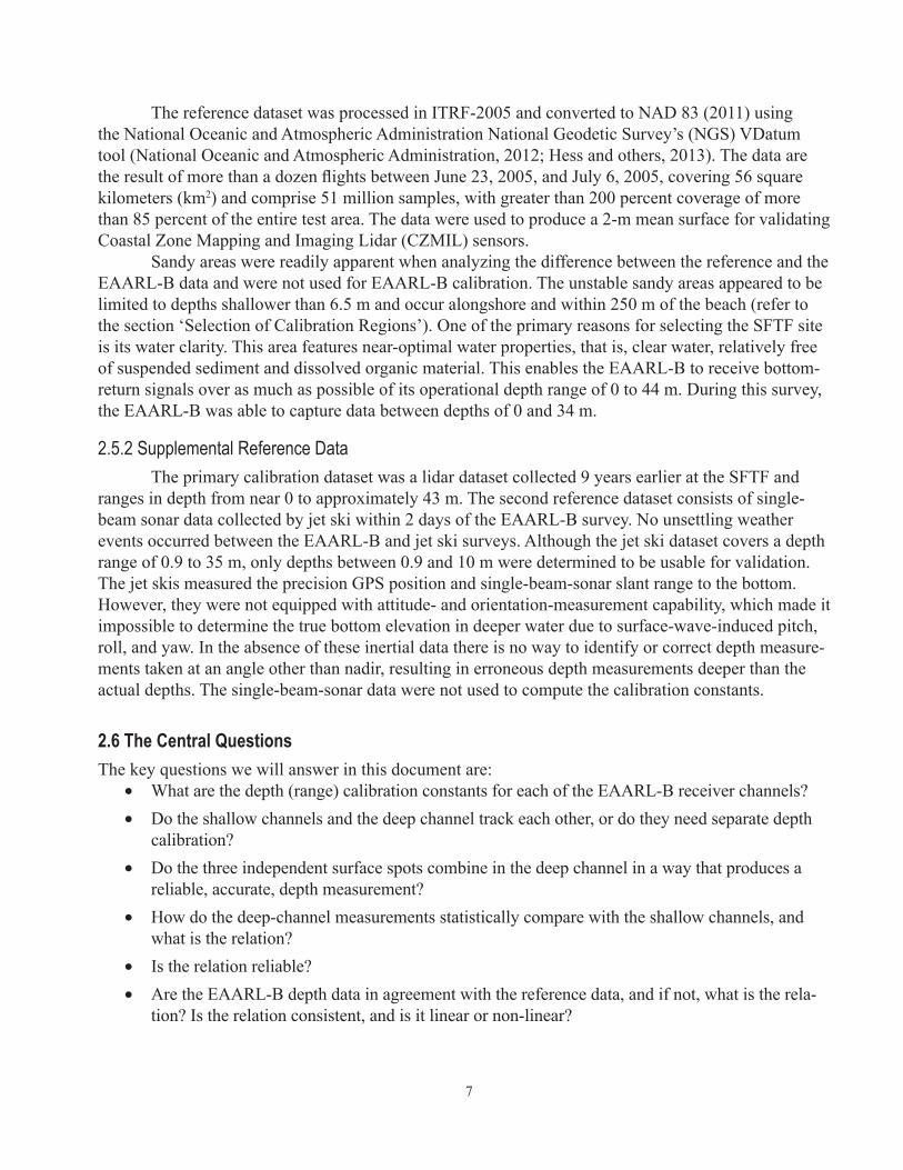
The reference dataset was processed in ITRF-2005 and converted to NAD 83 (2011) using the National Oceanic and Atmospheric Administration National Geodetic Survey’s (NGS) VDatum tool (National Oceanic and Atmospheric Administration, 2012; Hess and others, 2013). The data are the result of more than a dozen flights between June 23, 2005, and July 6, 2005, covering 56 square kilometers (km2) and comprise 51 million samples, with greater than 200 percent coverage of more than 85 percent of the entire test area. The data were used to produce a 2-m mean surface for validating Coastal Zone Mapping and Imaging Lidar (CZMIL) sensors.

Sandy areas were readily apparent when analyzing the difference between the reference and the EAARL-B data and were not used for EAARL-B calibration. The unstable sandy areas appeared to be limited to depths shallower than 6.5 m and occur alongshore and within 250 m of the beach (refer to the section ‘Selection of Calibration Regions’). One of the primary reasons for selecting the SFTF site is its water clarity. This area features near-optimal water properties, that is, clear water, relatively free of suspended sediment and dissolved organic material. This enables the EAARL-B to receive bottom-return signals over as much as possible of its operational depth range of 0 to 44 m. During this survey, the EAARL-B was able to capture data between depths of 0 and 34 m.

2.5.2 Supplemental Reference DataThe primary calibration dataset was a lidar dataset collected 9 years earlier at the SFTF and

ranges in depth from near 0 to approximately 43 m. The second reference dataset consists of single-beam sonar data collected by jet ski within 2 days of the EAARL-B survey. No unsettling weather events occurred between the EAARL-B and jet ski surveys. Although the jet ski dataset covers a depth range of 0.9 to 35 m, only depths between 0.9 and 10 m were determined to be usable for validation. The jet skis measured the precision GPS position and single-beam-sonar slant range to the bottom. However, they were not equipped with attitude- and orientation-measurement capability, which made it impossible to determine the true bottom elevation in deeper water due to surface-wave-induced pitch, roll, and yaw. In the absence of these inertial data there is no way to identify or correct depth measure-ments taken at an angle other than nadir, resulting in erroneous depth measurements deeper than the actual depths. The single-beam-sonar data were not used to compute the calibration constants.

2.6 The Central QuestionsThe key questions we will answer in this document are:

• What are the depth (range) calibration constants for each of the EAARL-B receiver channels?• Do the shallow channels and the deep channel track each other, or do they need separate depth

calibration?• Do the three independent surface spots combine in the deep channel in a way that produces a

reliable, accurate, depth measurement?• How do the deep-channel measurements statistically compare with the shallow channels, and

what is the relation?• Is the relation reliable?• Are the EAARL-B depth data in agreement with the reference data, and if not, what is the rela-

tion? Is the relation consistent, and is it linear or non-linear?

8

3. Methods

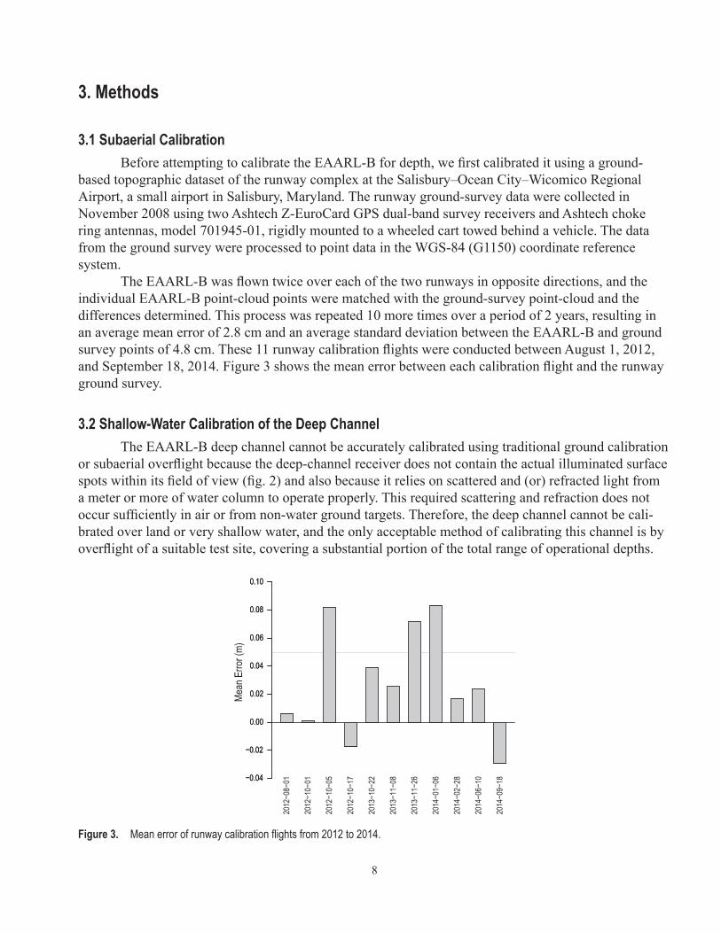
3.1 Subaerial CalibrationBefore attempting to calibrate the EAARL-B for depth, we first calibrated it using a ground-

based topographic dataset of the runway complex at the Salisbury–Ocean City–Wicomico Regional Airport, a small airport in Salisbury, Maryland. The runway ground-survey data were collected in November 2008 using two Ashtech Z-EuroCard GPS dual-band survey receivers and Ashtech choke ring antennas, model 701945-01, rigidly mounted to a wheeled cart towed behind a vehicle. The data from the ground survey were processed to point data in the WGS-84 (G1150) coordinate reference system.

The EAARL-B was flown twice over each of the two runways in opposite directions, and the individual EAARL-B point-cloud points were matched with the ground-survey point-cloud and the differences determined. This process was repeated 10 more times over a period of 2 years, resulting in an average mean error of 2.8 cm and an average standard deviation between the EAARL-B and ground survey points of 4.8 cm. These 11 runway calibration flights were conducted between August 1, 2012, and September 18, 2014. Figure 3 shows the mean error between each calibration flight and the runway ground survey.

3.2 Shallow-Water Calibration of the Deep ChannelThe EAARL-B deep channel cannot be accurately calibrated using traditional ground calibration

or subaerial overflight because the deep-channel receiver does not contain the actual illuminated surface spots within its field of view (fig. 2) and also because it relies on scattered and (or) refracted light from a meter or more of water column to operate properly. This required scattering and refraction does not occur sufficiently in air or from non-water ground targets. Therefore, the deep channel cannot be cali-brated over land or very shallow water, and the only acceptable method of calibrating this channel is by overflight of a suitable test site, covering a substantial portion of the total range of operational depths.

Figure 3. Mean error of runway calibration flights from 2012 to 2014.

2012−08−01

2012−10−01

2012−10−05

2012−10−17

2013−10−22

2013−11−08

2013−11−26

2014−01−06

2014−02−28

2014−06−10

2014−09−18

Mean

Erro

r (m)

−0.04

−0.02

0.00

0.02

0.04

0.06

0.08

0.10

−0.04

−0.02

0.00

0.02

0.04

0.06

0.08

0.10

9

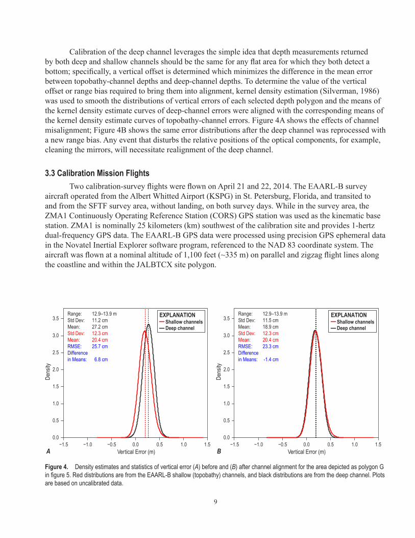
Calibration of the deep channel leverages the simple idea that depth measurements returned by both deep and shallow channels should be the same for any flat area for which they both detect a bottom; specifically, a vertical offset is determined which minimizes the difference in the mean error between topobathy-channel depths and deep-channel depths. To determine the value of the vertical offset or range bias required to bring them into alignment, kernel density estimation (Silverman, 1986) was used to smooth the distributions of vertical errors of each selected depth polygon and the means of the kernel density estimate curves of deep-channel errors were aligned with the corresponding means of the kernel density estimate curves of topobathy-channel errors. Figure 4A shows the effects of channel misalignment; Figure 4B shows the same error distributions after the deep channel was reprocessed with a new range bias. Any event that disturbs the relative positions of the optical components, for example, cleaning the mirrors, will necessitate realignment of the deep channel.

3.3 Calibration Mission FlightsTwo calibration-survey flights were flown on April 21 and 22, 2014. The EAARL-B survey

aircraft operated from the Albert Whitted Airport (KSPG) in St. Petersburg, Florida, and transited to and from the SFTF survey area, without landing, on both survey days. While in the survey area, the ZMA1 Continuously Operating Reference Station (CORS) GPS station was used as the kinematic base station. ZMA1 is nominally 25 kilometers (km) southwest of the calibration site and provides 1-hertz dual-frequency GPS data. The EAARL-B GPS data were processed using precision GPS ephemeral data in the Novatel Inertial Explorer software program, referenced to the NAD 83 coordinate system. The aircraft was flown at a nominal altitude of 1,100 feet (~335 m) on parallel and zigzag flight lines along the coastline and within the JALBTCX site polygon.

Figure 4. Density estimates and statistics of vertical error (A) before and (B) after channel alignment for the area depicted as polygon G in figure 5. Red distributions are from the EAARL-B shallow (topobathy) channels, and black distributions are from the deep channel. Plots are based on uncalibrated data.

−1.5 −1.0 −0.5 0.0 0.5 1.0 1.50.0

0.5

1.0

1.5

2.0

2.5

3.0

3.5

−1.5 −1.0 −0.5 0.0 0.5 1.0 1.50.0

0.5

1.0

1.5

2.0

2.5

3.0

3.5Range: 12.9–13.9 mStd Dev: 11.2 cmMean: 27.2 cmStd Dev: 12.3 cmMean: 20.4 cmRMSE: 25.7 cmDifference in Means: 6.8 cm

Range: 12.9–13.9 mStd Dev: 11.5 cmMean: 18.9 cmStd Dev: 12.3 cmMean: 20.4 cmRMSE: 23.3 cmDifference in Means: -1.4 cm

Vertical Error (m)

Dens

ity

Vertical Error (m)

Dens

ity

A B

Shallow channelsDeep channel

EXPLANATIONShallow channelsDeep channel

EXPLANATION

10

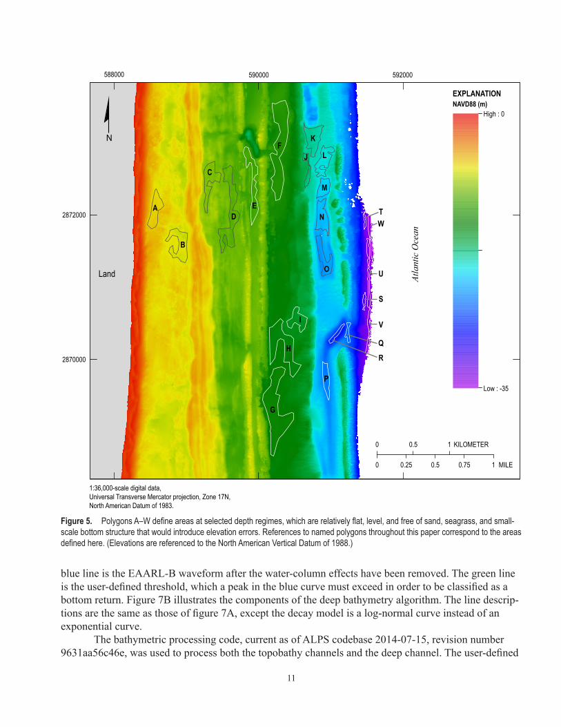
3.4 Selection of Calibration RegionsThe objective of this study was to calibrate the depth measurements made by the EAARL-B and

not to conduct an overall accuracy assessment of lidar performance in terms of horizontal accuracy or accuracy where there is significant submerged topographic relief, slope, or complex small-scale bottom structure. To facilitate optimal conditions for determining vertical error and depth-dependent offsets, the data were analyzed and polygons were delineated at 23 distinct depths ranging from 6.3 to 34 m. Each polygon was examined and analyzed for average depth, roughness, topographic complexity, levelness, flatness, and for overlap between the JALBTCX and EAARL-B surveys. Figure 5 shows the selected comparison regions.

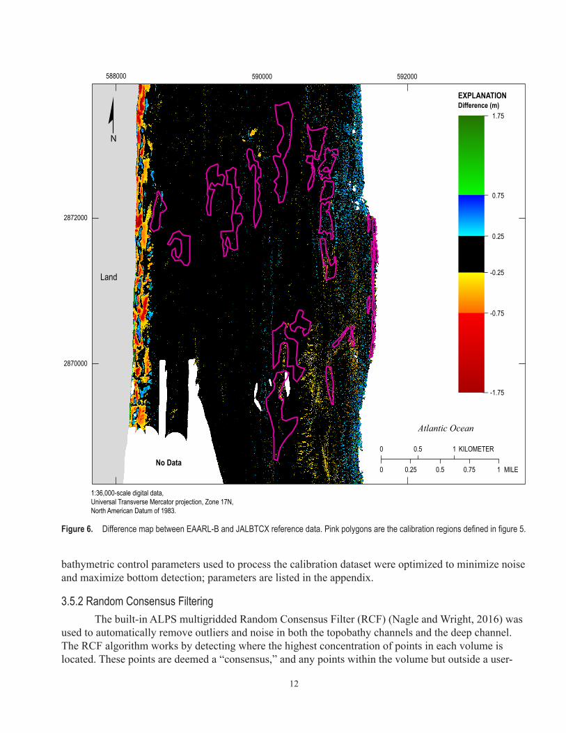
We were careful to select areas with minimal morphologic change, and we avoided areas with high relief, such as, spur-and-groove reefs, coral rubble, seagrass, and other complex small-scale bottom topography that could erroneously influence the depth-calibration measurements or cause range noise in either the EAARL-B or the JALBTCX reference dataset. Although there are plenty of data from both sensors between 0 and 6.5 m, all the data appeared to be sandy bottom and exhibited evidence of pronounced geomorphologic change, so those areas were excluded from the calibrations. Figure 6 is a difference map between calibrated EAARL-B and the reference dataset showing that areas of significant change (greater than ±25 cm) occur mostly within 250 m of the shoreline despite the 9-year time differ-ence between acquisition dates.

3.5 Data Processing, Filtering, and EditingThe EAARL-B is a full-waveform lidar system. The raw waveforms are composed of time and

intensity information, digitized at 1-nanosecond intervals, which must first be analyzed and processed to produce georeferenced point data specifying the precise 3-dimensional location of various surfaces of interest. For bathymetry, the surfaces of interest are the elevation of the seafloor and that of the water surface. After a raw point cloud is generated, it is passed through an automated filtering algorithm to remove random noise. The filtered point cloud is then edited by hand to remove systematic noise as well as any random noise missed by the automated filter. All these processing steps occur within the custom-built Airborne Lidar Processing System (ALPS) (Bonisteel and others, 2009), as does the point correspondence procedure central to this study.

3.5.1 Processing SoftwareThe three small field of view channels serve to measure topography and shallow-water

bathymetry. Three processing algorithms are used to convert the waveforms into point data—one for topography, one for bathymetry shallower than approximately 0.3 m depth (in clear water), and a third for deeper bathymetry. The same algorithm used to process deeper bathymetry from the three topobathy channels is used with different parameters to process bathymetry from the deep channel.

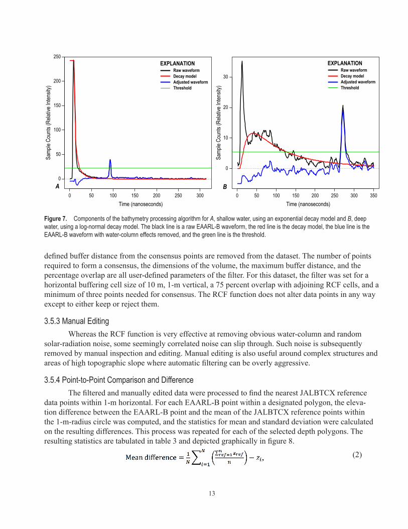
The depth-detection algorithm subtracts a user-defined normalized water-column model from each raw waveform. The model can be either a combination of exponential decays representing the laser and the water, or it can be a fitted normalized log-normal function. Once the water-column effects are removed, potential bottom peaks are threshold detected and then further analyzed for expected bottom return-pulse characteristics, including pulse width, rise, and fall times. If the bottom return is accepted, it is returned as a valid bottom signal.

Figure 7A illustrates the components of the topobathy-channel bottom detection algorithm where the black line is a single raw EAARL-B waveform, the red line is the exponential decay model, and the

11

blue line is the EAARL-B waveform after the water-column effects have been removed. The green line is the user-defined threshold, which a peak in the blue curve must exceed in order to be classified as a bottom return. Figure 7B illustrates the components of the deep bathymetry algorithm. The line descrip-tions are the same as those of figure 7A, except the decay model is a log-normal curve instead of an exponential curve.

The bathymetric processing code, current as of ALPS codebase 2014-07-15, revision number 9631aa56c46e, was used to process both the topobathy channels and the deep channel. The user-defined

Figure 5. Polygons A–W define areas at selected depth regimes, which are relatively flat, level, and free of sand, seagrass, and small-scale bottom structure that would introduce elevation errors. References to named polygons throughout this paper correspond to the areas defined here. (Elevations are referenced to the North American Vertical Datum of 1988.)

Atla

ntic

Oce

an

Land

NAVD88 (m)High : 0

Low : -35

0 0.5 1 KILOMETER

0 0.25 0.5 0.75 1 MILE

F

G

H

D

I

E

B

K

L

C

AN

O

P

M

J

U

V

W

R

Q

S

T

588000 590000 592000

2870000

2872000

1:36,000-scale digital data, Universal Transverse Mercator projection, Zone 17N, North American Datum of 1983.

N

EXPLANATION

12

bathymetric control parameters used to process the calibration dataset were optimized to minimize noise and maximize bottom detection; parameters are listed in the appendix.

3.5.2 Random Consensus FilteringThe built-in ALPS multigridded Random Consensus Filter (RCF) (Nagle and Wright, 2016) was

used to automatically remove outliers and noise in both the topobathy channels and the deep channel. The RCF algorithm works by detecting where the highest concentration of points in each volume is located. These points are deemed a “consensus,” and any points within the volume but outside a user-

Figure 6. Difference map between EAARL-B and JALBTCX reference data. Pink polygons are the calibration regions defined in figure 5.

Atlantic Ocean

Land

EXPLANATION

No Data

Difference (m)

0 0.5 1 KILOMETER

0 0.25 0.5 0.75 1 MILE

588000 590000 592000

2870000

2872000

1:36,000-scale digital data, Universal Transverse Mercator projection, Zone 17N, North American Datum of 1983.

1.75

0.75

0.25

-0.25

-0.75

-1.75

N

13

defined buffer distance from the consensus points are removed from the dataset. The number of points required to form a consensus, the dimensions of the volume, the maximum buffer distance, and the percentage overlap are all user-defined parameters of the filter. For this dataset, the filter was set for a horizontal buffering cell size of 10 m, 1-m vertical, a 75 percent overlap with adjoining RCF cells, and a minimum of three points needed for consensus. The RCF function does not alter data points in any way except to either keep or reject them.

3.5.3 Manual EditingWhereas the RCF function is very effective at removing obvious water-column and random

solar-radiation noise, some seemingly correlated noise can slip through. Such noise is subsequently removed by manual inspection and editing. Manual editing is also useful around complex structures and areas of high topographic slope where automatic filtering can be overly aggressive.

3.5.4 Point-to-Point Comparison and DifferenceThe filtered and manually edited data were processed to find the nearest JALBTCX reference

data points within 1-m horizontal. For each EAARL-B point within a designated polygon, the eleva-tion difference between the EAARL-B point and the mean of the JALBTCX reference points within the 1-m-radius circle was computed, and the statistics for mean and standard deviation were calculated on the resulting differences. This process was repeated for each of the selected depth polygons. The resulting statistics are tabulated in table 3 and depicted graphically in figure 8.

(2)

Figure 7. Components of the bathymetry processing algorithm for A, shallow water, using an exponential decay model and B, deep water, using a log-normal decay model. The black line is a raw EAARL-B waveform, the red line is the decay model, the blue line is the EAARL-B waveform with water-column effects removed, and the green line is the threshold.

0 50 100 150 200 250 300 350

0

10

20

30

Time (nanoseconds)

Samp

le Co

unts

(Rela

tive I

ntens

ity)

0 50 100 150 200 250 300

0

50

100

150

200

250

Time (nanoseconds)

Samp

le Co

unts

(Rela

tive I

ntens

ity)

A B

Raw waveformEXPLANATION

Decay modelAdjusted waveformThreshold

Raw waveformEXPLANATION

Decay modelAdjusted waveformThreshold

14

where

n is the number of reference dataset points in a 1-m circle around an EAARL-B data point;

zref is the elevation of a reference dataset point;

N is the number of EAARL-B points; and

zi is the elevation of an EAARL-B data point.

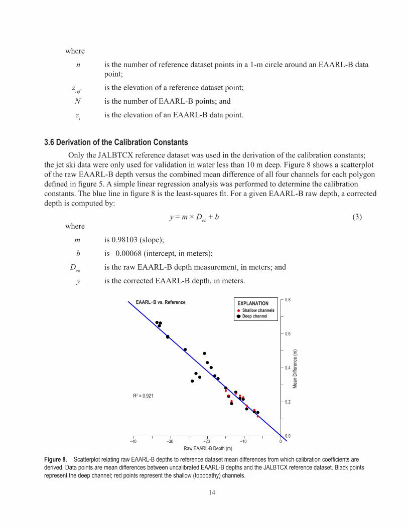
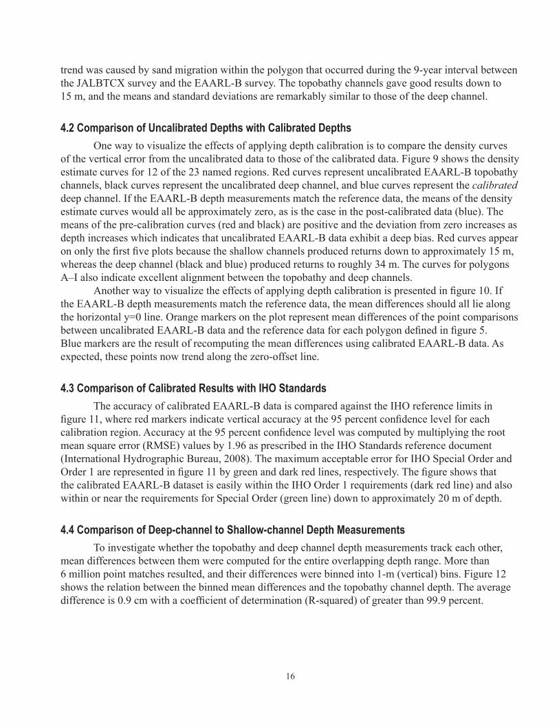
3.6 Derivation of the Calibration ConstantsOnly the JALBTCX reference dataset was used in the derivation of the calibration constants;

the jet ski data were only used for validation in water less than 10 m deep. Figure 8 shows a scatterplot of the raw EAARL-B depth versus the combined mean difference of all four channels for each polygon defined in figure 5. A simple linear regression analysis was performed to determine the calibration constants. The blue line in figure 8 is the least-squares fit. For a given EAARL-B raw depth, a corrected depth is computed by:

y = m × Deb + b (3)where

m is 0.98103 (slope);

b is –0.00068 (intercept, in meters);

Deb is the raw EAARL-B depth measurement, in meters; and

y is the corrected EAARL-B depth, in meters.

Figure 8. Scatterplot relating raw EAARL-B depths to reference dataset mean differences from which calibration coefficients are derived. Data points are mean differences between uncalibrated EAARL-B depths and the JALBTCX reference dataset. Black points represent the deep channel; red points represent the shallow (topobathy) channels.

0.0

0.2

0.4

0.6

0.8

−40 −30 −20 −10 0

EAARL−B vs. Reference

Raw EAARL-B Depth (m)

R2 = 0.921

Mean

Diffe

renc

e (m)

EXPLANATIONShallow channelsDeep channel

15

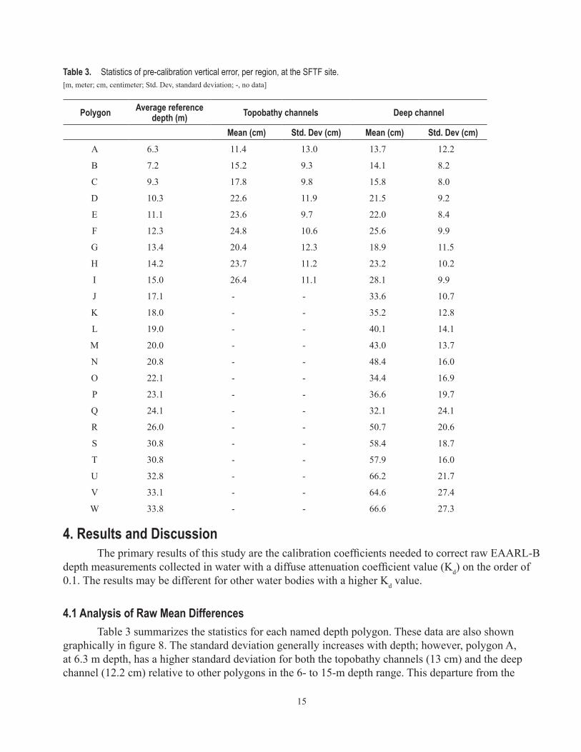
Table 3. Statistics of pre-calibration vertical error, per region, at the SFTF site.[m, meter; cm, centimeter; Std. Dev, standard deviation; -, no data]

Polygon Average reference depth (m) Topobathy channels Deep channel

Mean (cm) Std. Dev (cm) Mean (cm) Std. Dev (cm)A 6.3 11.4 13.0 13.7 12.2

B 7.2 15.2 9.3 14.1 8.2

C 9.3 17.8 9.8 15.8 8.0

D 10.3 22.6 11.9 21.5 9.2

E 11.1 23.6 9.7 22.0 8.4

F 12.3 24.8 10.6 25.6 9.9

G 13.4 20.4 12.3 18.9 11.5

H 14.2 23.7 11.2 23.2 10.2

I 15.0 26.4 11.1 28.1 9.9

J 17.1 - - 33.6 10.7

K 18.0 - - 35.2 12.8

L 19.0 - - 40.1 14.1

M 20.0 - - 43.0 13.7

N 20.8 - - 48.4 16.0

O 22.1 - - 34.4 16.9

P 23.1 - - 36.6 19.7

Q 24.1 - - 32.1 24.1

R 26.0 - - 50.7 20.6

S 30.8 - - 58.4 18.7

T 30.8 - - 57.9 16.0

U 32.8 - - 66.2 21.7

V 33.1 - - 64.6 27.4

W 33.8 - - 66.6 27.3

4. Results and DiscussionThe primary results of this study are the calibration coefficients needed to correct raw EAARL-B

depth measurements collected in water with a diffuse attenuation coefficient value (Kd) on the order of 0.1. The results may be different for other water bodies with a higher Kd value.

4.1 Analysis of Raw Mean DifferencesTable 3 summarizes the statistics for each named depth polygon. These data are also shown

graphically in figure 8. The standard deviation generally increases with depth; however, polygon A, at 6.3 m depth, has a higher standard deviation for both the topobathy channels (13 cm) and the deep channel (12.2 cm) relative to other polygons in the 6- to 15-m depth range. This departure from the

16

trend was caused by sand migration within the polygon that occurred during the 9-year interval between the JALBTCX survey and the EAARL-B survey. The topobathy channels gave good results down to 15 m, and the means and standard deviations are remarkably similar to those of the deep channel.

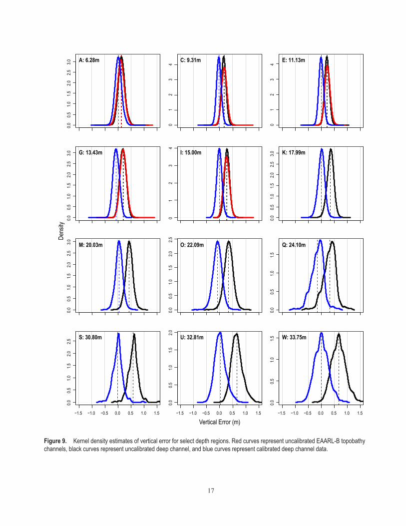
4.2 Comparison of Uncalibrated Depths with Calibrated DepthsOne way to visualize the effects of applying depth calibration is to compare the density curves

of the vertical error from the uncalibrated data to those of the calibrated data. Figure 9 shows the density estimate curves for 12 of the 23 named regions. Red curves represent uncalibrated EAARL-B topobathy channels, black curves represent the uncalibrated deep channel, and blue curves represent the calibrated deep channel. If the EAARL-B depth measurements match the reference data, the means of the density estimate curves would all be approximately zero, as is the case in the post-calibrated data (blue). The means of the pre-calibration curves (red and black) are positive and the deviation from zero increases as depth increases which indicates that uncalibrated EAARL-B data exhibit a deep bias. Red curves appear on only the first five plots because the shallow channels produced returns down to approximately 15 m, whereas the deep channel (black and blue) produced returns to roughly 34 m. The curves for polygons A–I also indicate excellent alignment between the topobathy and deep channels.

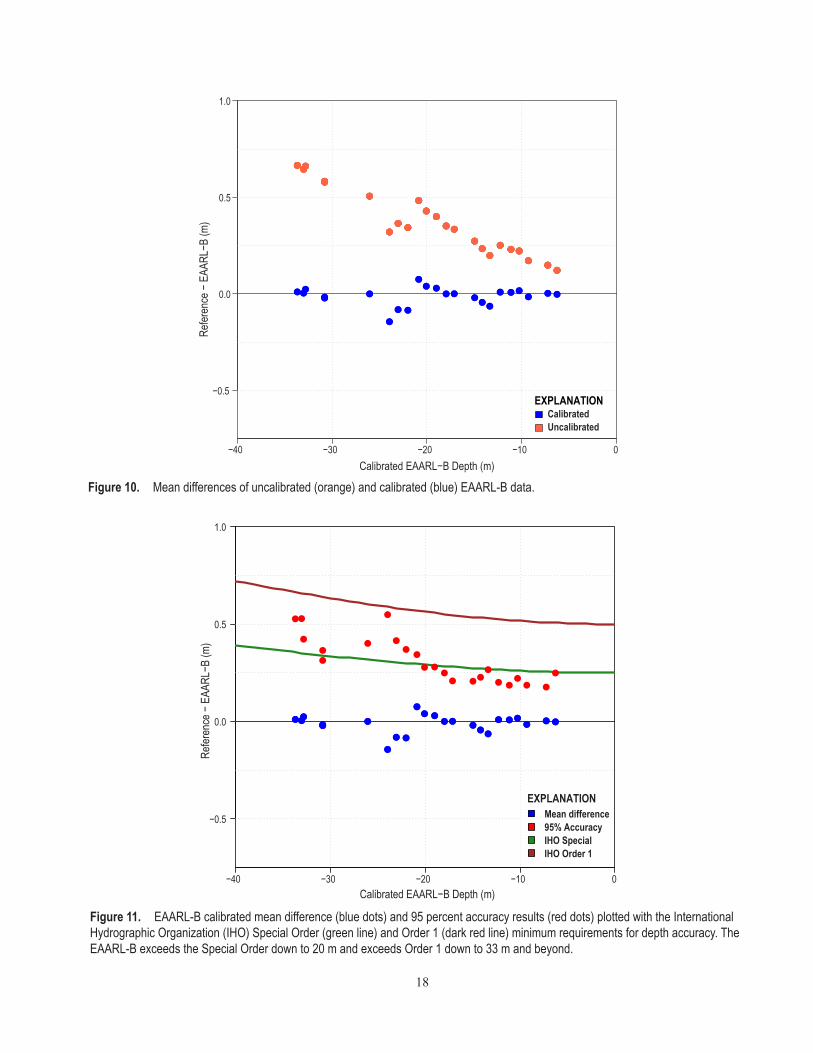
Another way to visualize the effects of applying depth calibration is presented in figure 10. If the EAARL-B depth measurements match the reference data, the mean differences should all lie along the horizontal y=0 line. Orange markers on the plot represent mean differences of the point comparisons between uncalibrated EAARL-B data and the reference data for each polygon defined in figure 5. Blue markers are the result of recomputing the mean differences using calibrated EAARL-B data. As expected, these points now trend along the zero-offset line.

4.3 Comparison of Calibrated Results with IHO StandardsThe accuracy of calibrated EAARL-B data is compared against the IHO reference limits in

figure 11, where red markers indicate vertical accuracy at the 95 percent confidence level for each calibration region. Accuracy at the 95 percent confidence level was computed by multiplying the root mean square error (RMSE) values by 1.96 as prescribed in the IHO Standards reference document (International Hydrographic Bureau, 2008). The maximum acceptable error for IHO Special Order and Order 1 are represented in figure 11 by green and dark red lines, respectively. The figure shows that the calibrated EAARL-B dataset is easily within the IHO Order 1 requirements (dark red line) and also within or near the requirements for Special Order (green line) down to approximately 20 m of depth.

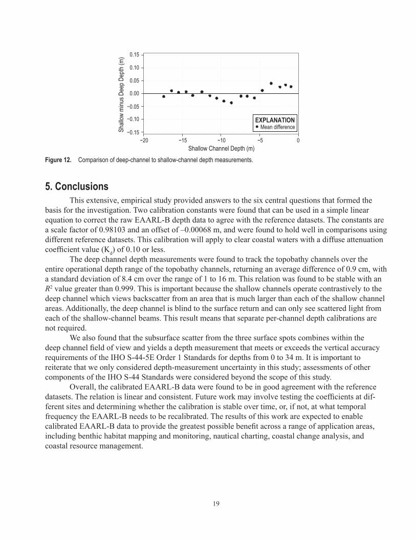
4.4 Comparison of Deep-channel to Shallow-channel Depth MeasurementsTo investigate whether the topobathy and deep channel depth measurements track each other,

mean differences between them were computed for the entire overlapping depth range. More than 6 million point matches resulted, and their differences were binned into 1-m (vertical) bins. Figure 12 shows the relation between the binned mean differences and the topobathy channel depth. The average difference is 0.9 cm with a coefficient of determination (R-squared) of greater than 99.9 percent.

17

Figure 9. Kernel density estimates of vertical error for select depth regions. Red curves represent uncalibrated EAARL-B topobathy channels, black curves represent uncalibrated deep channel, and blue curves represent calibrated deep channel data.

A: 6.28m C: 9.31m E: 11.13m

G: 13.43m I: 15.00m K: 17.99m

M: 20.03m O: 22.09m Q: 24.10m

S: 30.80m U: 32.81m W: 33.75m

0.00.5

1.01.5

2.02.5

3.00.0

0.51.0

1.52.0

2.53.0

0.00.5

1.01.5

2.02.5

3.0

0.00.5

1.01.5

2.02.5

3.0

0.00.5

1.01.5

2.02.5

0.00.5

1.01.5

−1.5 −1.0 −0.5 0.0 0.5 1.0 1.5

0.00.5

1.01.5

2.02.5

−1.5 −1.0 −0.5 0.0 0.5 1.0 1.5

0.00.5

1.01.5

2.00

12

34

01

23

4

01

23

4

−1.5 −1.0 −0.5 0.0 0.5 1.0 1.5

0.00.5

1.01.5

Dens

ity

Vertical Error (m)

18

Figure 11. EAARL-B calibrated mean difference (blue dots) and 95 percent accuracy results (red dots) plotted with the International Hydrographic Organization (IHO) Special Order (green line) and Order 1 (dark red line) minimum requirements for depth accuracy. The EAARL-B exceeds the Special Order down to 20 m and exceeds Order 1 down to 33 m and beyond.

Figure 10. Mean differences of uncalibrated (orange) and calibrated (blue) EAARL-B data.

CalibratedUncalibrated

EXPLANATION

−40 −30 −20 −10 0

−0.5

0.0

0.5

1.0

Calibrated EAARL−B Depth (m)

Refer

ence

− E

AARL

−B (m

)

−40 −30 −20 −10 0

−0.5

0.0

0.5

1.0

Calibrated EAARL−B Depth (m)

Refer

ence

− E

AARL

−B (m

)

Mean difference95% AccuracyIHO SpecialIHO Order 1

EXPLANATION

19

5. ConclusionsThis extensive, empirical study provided answers to the six central questions that formed the

basis for the investigation. Two calibration constants were found that can be used in a simple linear equation to correct the raw EAARL-B depth data to agree with the reference datasets. The constants are a scale factor of 0.98103 and an offset of –0.00068 m, and were found to hold well in comparisons using different reference datasets. This calibration will apply to clear coastal waters with a diffuse attenuation coefficient value (Kd) of 0.10 or less.

The deep channel depth measurements were found to track the topobathy channels over the entire operational depth range of the topobathy channels, returning an average difference of 0.9 cm, with a standard deviation of 8.4 cm over the range of 1 to 16 m. This relation was found to be stable with an R2 value greater than 0.999. This is important because the shallow channels operate contrastively to the deep channel which views backscatter from an area that is much larger than each of the shallow channel areas. Additionally, the deep channel is blind to the surface return and can only see scattered light from each of the shallow-channel beams. This result means that separate per-channel depth calibra tions are not required.

We also found that the subsurface scatter from the three surface spots combines within the deep channel field of view and yields a depth measurement that meets or exceeds the vertical accuracy re quirements of the IHO S-44-5E Order 1 Standards for depths from 0 to 34 m. It is important to reiterate that we only considered depth-measurement uncertainty in this study; assessments of other components of the IHO S-44 Standards were considered beyond the scope of this study.

Overall, the calibrated EAARL-B data were found to be in good agreement with the reference datasets. The relation is linear and consistent. Future work may involve testing the coefficients at dif-ferent sites and determining whether the calibration is stable over time, or, if not, at what temporal frequency the EAARL-B needs to be recalibrated. The results of this work are expected to enable calibrated EAARL-B data to provide the greatest possible benefit across a range of application areas, including benthic habitat mapping and monitoring, nautical charting, coastal change analysis, and coastal resource management.

Figure 12. Comparison of deep-channel to shallow-channel depth measurements.

−20 −15 −10 −5 0−0.15

−0.05

−0.10

0.00

0.10

0.15

0.05

● Mean difference

Shallow Channel Depth (m)

Shall

ow m

inus D

eep D

epth

(m)

EXPLANATION

20

6. References CitedBonisteel, J.M., Nayegandhi, Amar, Wright, C.W., Brock, J.C., and Nagle, D.B., 2009, Experimental Advanced

Airborne Research Lidar (EAARL) data processing manual: U.S. Geological Survey Open-File Report 2009–1078, 38 p.

Ford, T.J., and Hamilton, J., 2003, A new positioning filter—Phase smoothing in the position domain, naviga-tion: Journal of The Institute of Navigation, v. 50, no. 2, p. 65–78.

Grewal, M.S., Andrews, A.P., and Bartone, C.G., 2013, Global navigation satellite systems, inertial navigation, and integration (3d ed.): Hoboken, N.J., Wiley, 608 p.

Guenther, G.C., LaRocque, P.E., and Lillycrop, W.J., 1994, Multiple surface channels in Scanning Hydrographic Operational Airborne Lidar Survey (SHOALS) airborne lidar: Proceedings of SPIE, Ocean Optics XII, v. 2258, p. 422–430, accessed January 19, 2015, at http://dx.doi.org/10.1117/12.190084.

Guenther, G.C., Thomas, R.W.L., and LaRocque, P.E., 1996, Design considerations for achieving high accuracy with the SHOALS bathymetric lidar system: Proceedings of SPIE, Laser Remote Sensing of Natural Water—From Theory to Practice, v. 2964, p. 54−71, accessed January 19, 2015, at http://dx.doi.org/10.1117/12.258353.

Hamamatsu Photonics K.K., 2007, Photomultiplier tubes, Basics and applications (3d ed.): Hamamatsu Photon-ics K.K., 323 p.

Hess, K., Jeong, I., and White, S., 2013, Revised VDatum for eastern Florida: National Oceanographic and At-mospheric Administration Technical Memorandum NOS CS 30, 49 p.

International Hydrographic Bureau, 2008, IHO Standards for hydrographic surveys (5th ed.): International Hy-drographic Organization Special Publication No. 44, 36 p. [Also available at http://www.iho.int/iho_pubs/standard/S-44_5E.pdf.]

Irish, J.L., and Lillycrop, W.J., 1999, Scanning laser mapping of the coastal zone—The SHOALS system: ISPRS Journal of Photogrammetry and Remote Sensing, v. 54, no. 2–3, p. 123–129., accessed January 20, 2015, at http://dx.doi.org/10.1016/S0924-2716(99)00003-9.

Laser Institute of America, 2007, American National Standard for safe use of lasers: American National Stan-dards Institute ANSI Z136.1–2007, 22 p. [Also available at https://www.lia.org/PDF/Z136_1_s.pdf.]

Long, B., Cottin, A., and Collin, A., 2007, What Optech’s bathymetric lidar sees underwater, in Proceedings of IEEE International Geoscience and Remote Sensing Symposium, IGARSS 2007, Barcelona, Spain, p. 3170–3173.

Nagle, D.B., and Wright, C.W., 2016, Algorithms used in the Airborne Lidar Processing System (ALPS): U.S. Geological Survey Open-File Report, 45 p., http://dx.doi.org/10.3133/20161046.

National Oceanic and Atmospheric Administration, 2007, Topographic and Bathymetric data considerations: Datum, Datum Conversion Techniques, and Data Integration, 2007, Part II of A Roadmap to a Seamless Topobathy Surface, National Oceanographic and Atmospheric Administration Technical Report NOAA/CSC/20718-PUB, 25 p.

National Oceanic and Atmospheric Administration, 2012, VDatum manual for development and support of NOAA’s vertical datum transformation tool, VDatum, version 1.01, 127 p., accessed January 21, 2015, at http://www.nauticalcharts.noaa.gov/csdl/publications/Manual_2012.06.26.doc.

Silverman, B.W., 1986, Density estimation for statistics and data analysis: London, Chapman and Hall/CRC, 176 p.Wright, C.W., and Brock, J.C., 2002, EAARL—A lidar for mapping shallow coral reefs and other coastal en-

vironments, in Proceedings of the 7th International Conference on Remote Sensing for Marine and Coastal Environments, Miami, Fla., U.S.A., CD-ROM.

21

7. Appendix 1

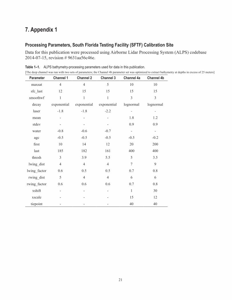
Processing Parameters, South Florida Testing Facility (SFTF) Calibration SiteData for this publication were processed using Airborne Lidar Processing System (ALPS) codebase 2014-07-15, revision # 9631aa56c46e.

Table 1–1. ALPS bathymetry-processing parameters used for data in this publication.[The deep channel was run with two sets of parameters; the Channel 4b parameter set was optimized to extract bathymetry at depths in excess of 25 meters]

Parameter Channel 1 Channel 2 Channel 3 Channel 4a Channel 4bmaxsat 4 4 5 10 10

sfc_last 12 15 15 15 15

smoothwf 1 1 1 3 3

decay exponential exponential exponential lognormal lognormal

laser -1.8 -1.8 -2.2 - -

mean - - - 1.8 1.2

stdev - - - 0.9 0.9

water -0.8 -0.6 -0.7 - -

agc -0.5 -0.5 -0.5 -0.5 -0.2

first 10 14 12 20 200

last 185 182 161 400 400

thresh 3 3.9 5.5 5 3.5

lwing_dist 4 4 4 7 9

lwing_factor 0.6 0.5 0.5 0.7 0.8

rwing_dist 5 4 4 6 6

rwing_factor 0.6 0.6 0.6 0.7 0.8

xshift - - - 1 30

xscale - - - 15 12

tiepoint - - - 40 40

22

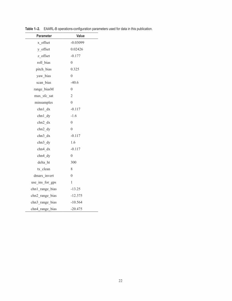
Table 1–2. EAARL-B operations-configuration parameters used for data in this publication.

Parameter Valuex_offset -0.03099

y_offset 0.02426

z_offset -0.177

roll_bias 0

pitch_bias 0.325

yaw_bias 0

scan_bias -40.6

range_biasM 0

max_sfc_sat 2

minsamples 0

chn1_dx -0.117

chn1_dy -1.6

chn2_dx 0

chn2_dy 0

chn3_dx -0.117

chn3_dy 1.6

chn4_dx -0.117

chn4_dy 0

delta_ht 300

tx_clean 8

dmars_invert 0

use_ins_for_gps 1

chn1_range_bias -13.25

chn2_range_bias -12.375

chn3_range_bias -10.564

chn4_range_bias -20.475

Wright and others—

Depth Calibration of the Experimental Advanced Airborne Research Lidar, EAARL-B—Open-File Report 2016–1048

ISSN 2331-1258 (online)http://dx.doi.org/10.3133/ofr20161048