Depth and Transient Imaging with Compressive SPAD Array Cameras

Qilin Sun1 Xiong Dun1 Yifan Peng2,1 Wolfgang Heidrich1

1KAUST 2University of British Columbia

Abstract

Time-of-flight depth imaging and transient imaging aretwo imaging modalities that have recently received a lot ofinterest. Despite much research, existing hardware systemsare limited either in terms of temporal resolution or areprohibitively expensive. Arrays of Single Photon AvalancheDiodes (SPADs) promise to fill this gap by providing highertemporal resolution at an affordable cost. UnfortunatelySPAD arrays are to date only available in relatively smallresolutions.

In this work we aim to overcome the spatial resolutionlimit of SPAD arrays by employing a compressive sens-ing camera design. Using a DMD and custom optics, weachieve an image resolution of up to 800×400 on SPAD Ar-rays of resolution 64×32. Using our new data fitting modelfor the time histograms, we suppress the noise while ab-stracting the phase and amplitude information, so as to re-alize a temporal resolution of a few tens of picoseconds.

1. Introduction

Time-resolved imaging of light propagation effects hasin recent years become a major research direction. Fromthe now ubiquitous continuous wave ToF and RGB-D cam-eras, to more complex analysis of transient effects such aslight-in-flight imaging [1, 47, 23], looking around the cor-ner [21, 46, 24], or imaging in scattering media [14, 34, 25]the applications of high speed light transport analysis arevast.

Unfortunately, work on these problems has been ham-pered by hardware limitations. On the consumer end, in-expensive time of flight cameras are available for a fewhundred dollars, but they provide a limited temporal resolu-tion owing to modulation frequencies of only 10-130 MHz.On the high end, the combination of fast lasers and streakcameras provides temporal resolutions in the single digit pi-cosecond range, but at a cost that is 2-3 orders of magni-tude higher. Recently, single photon avalanche diodes havestarted to emerge as an alternative hardware solution thatfills the gap both in terms of resolution and cost. SPADsare also attractive for their ability to detect very small sig-

nals, i.e. single photons. Unfortunately, image sensors builtaround SPAD technologies currently still suffer from lowspatial resolution (e.g. 64× 32 pixels).

In our work we aim to overcome the spatial resolutionlimit of SPAD arrays while preserving and even enhanc-ing the time resolution by developing a compressive sensingSPAD camera. Since SPADs work with small signals thatare inherently noisy, and compressive sensing is well knownto amplify noise, devising such a compressive SPAD cam-era not only requires significant innovation on the camerahardware, but also a number of algorithmic contributions.Specifically, our contributions include

• the design and prototyping of a compact optical systemcontaining imaging and re-imaging optics, as well as aDMD-based active modulation component.

• fill factor improvements of conventional SPAD sensorsto enable the compressive sensing scenario by embed-ding a diffractive micro lens array (DMLA) in front ofthe bare sensors.

• inverse problem formulation to reconstruct high reso-lution 3D volumes from captured SPAD data.

• proposing a temporal PSF model based on the RC gateswitching behavior of the electronics, and using it todeconvolve and sharpen the time profile of the tran-sient image, achieving a temporal resolution in therange of tens of picoseconds.

• analysis and correction for phase distortions on theSPAD array caused by on-chip signal propagation dif-ferences.

2. Related WorkTime-of-Flight Cameras Continuous wave ToF camerasuse the correlation between a sinusoidally modulated illu-mination source and a reference signal to measure the timedelay due to light propagation [41, 38]. These types of cam-eras have been widely adapted in computer vision in theform of depth and RGB-D cameras. Recently, researchershave found new and exciting uses of this type of hardwarebeyond simple depth imaging, including transient imaging

1

Microlens Array

SPAD

Random Pattern

(a) Picosecond laser

(e) Reimaging

lens

(b) Imaging lens

(c) DMD

(d) TIR Prism

(f) SPAD array

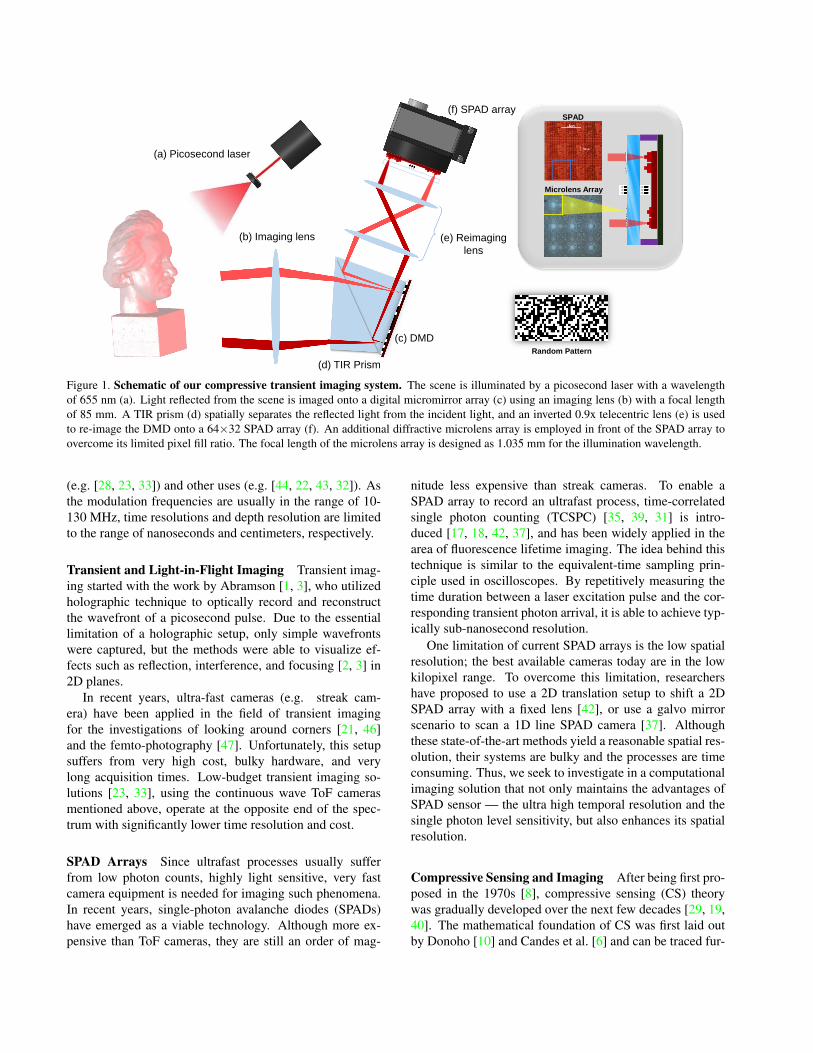
Figure 1. Schematic of our compressive transient imaging system. The scene is illuminated by a picosecond laser with a wavelengthof 655 nm (a). Light reflected from the scene is imaged onto a digital micromirror array (c) using an imaging lens (b) with a focal lengthof 85 mm. A TIR prism (d) spatially separates the reflected light from the incident light, and an inverted 0.9x telecentric lens (e) is usedto re-image the DMD onto a 64×32 SPAD array (f). An additional diffractive microlens array is employed in front of the SPAD array toovercome its limited pixel fill ratio. The focal length of the microlens array is designed as 1.035 mm for the illumination wavelength.

(e.g. [28, 23, 33]) and other uses (e.g. [44, 22, 43, 32]). Asthe modulation frequencies are usually in the range of 10-130 MHz, time resolutions and depth resolution are limitedto the range of nanoseconds and centimeters, respectively.

Transient and Light-in-Flight Imaging Transient imag-ing started with the work by Abramson [1, 3], who utilizedholographic technique to optically record and reconstructthe wavefront of a picosecond pulse. Due to the essentiallimitation of a holographic setup, only simple wavefrontswere captured, but the methods were able to visualize ef-fects such as reflection, interference, and focusing [2, 3] in2D planes.

In recent years, ultra-fast cameras (e.g. streak cam-era) have been applied in the field of transient imagingfor the investigations of looking around corners [21, 46]and the femto-photography [47]. Unfortunately, this setupsuffers from very high cost, bulky hardware, and verylong acquisition times. Low-budget transient imaging so-lutions [23, 33], using the continuous wave ToF camerasmentioned above, operate at the opposite end of the spec-trum with significantly lower time resolution and cost.

SPAD Arrays Since ultrafast processes usually sufferfrom low photon counts, highly light sensitive, very fastcamera equipment is needed for imaging such phenomena.In recent years, single-photon avalanche diodes (SPADs)have emerged as a viable technology. Although more ex-pensive than ToF cameras, they are still an order of mag-

nitude less expensive than streak cameras. To enable aSPAD array to record an ultrafast process, time-correlatedsingle photon counting (TCSPC) [35, 39, 31] is intro-duced [17, 18, 42, 37], and has been widely applied in thearea of fluorescence lifetime imaging. The idea behind thistechnique is similar to the equivalent-time sampling prin-ciple used in oscilloscopes. By repetitively measuring thetime duration between a laser excitation pulse and the cor-responding transient photon arrival, it is able to achieve typ-ically sub-nanosecond resolution.

One limitation of current SPAD arrays is the low spatialresolution; the best available cameras today are in the lowkilopixel range. To overcome this limitation, researchershave proposed to use a 2D translation setup to shift a 2DSPAD array with a fixed lens [42], or use a galvo mirrorscenario to scan a 1D line SPAD camera [37]. Althoughthese state-of-the-art methods yield a reasonable spatial res-olution, their systems are bulky and the processes are timeconsuming. Thus, we seek to investigate in a computationalimaging solution that not only maintains the advantages ofSPAD sensor — the ultra high temporal resolution and thesingle photon level sensitivity, but also enhances its spatialresolution.

Compressive Sensing and Imaging After being first pro-posed in the 1970s [8], compressive sensing (CS) theorywas gradually developed over the next few decades [29, 19,40]. The mathematical foundation of CS was first laid outby Donoho [10] and Candes et al. [6] and can be traced fur-

ther back to sparse recovery works [13, 12, 11]. After thesingle pixel camera [15] had been invented, it became possi-ble to replace conventional sampling and reconstruction op-erations with a more general linear measurement schemescoupled with optimization methods [9, 16, 36]. CS ap-proaches are particularly beneficial in scenarios where highresolution sensor arrays are either technologically infeasibleor prohibitively expensive, as is the case for SPAD sensors.For instance, a mask shifting camera [48] and a CS-basedinfra-red camera [7] have been realized. These works in-spire us to apply CS approach into transient or depth imag-ing to acquire high frequency spatial information.

3. System OverviewOur imaging system is an integration of optics, mechan-

ics, electronics, and computation, as illustrated in Figure 1.The key components of the the hardware setup are a SPADarray with a resolution of (n=64)×(m=32) pixels that pro-vides a high temporal resolution in combination with illu-mination from a picosecond laser, as well as a Digital Mi-cromirror Device (DMD) in combination with re-imagingoptics that achieve improved spatial resolution through acompressive sensing approach. In the following we explainthe high level operation of the system by examining the spa-tial and temporal resolution characteristics.

The Temporal Resolution of the system is determinedby the ability to measure time delays between the emissionof a pulse by the the picosecond laser, and the time the re-flected light is received at the SPAD array. For a given ex-posure interval, called the gate width, which can be as shortas 200ps, each SPAD pixel reports whether or not a photonwas received during this time interval. Moreover, the starttime of the exposure interval can be shifted with a preci-sion of 20ps. By repeatedly emitting pulses from the laserwhile adjusting this time offset, we can sample the transientpropagation of light in the scene. In our case, the SPADarray was operated in TCSPC mode with 20ps shift per cir-cle and 830ps gate width to improve the light efficiency ofthe system compared to the shortest gate width of 200ps.Although this gate width should normally limit the tempo-ral resolution of the system, we show in Section 4.3 how tosuppress the low-pass effect of the gate signal and recovera temporal resolution in the 10s of picoseconds. We notethat, since each measurement is a binary event, measure-ments need to be repeated multiple times to reduce noiseand obtain estimates of intensity for each phase delay.

The Spatial Resolution of the system is primarily deter-mined by the resolution of the DMD instead of the muchlower resolution of the SPAD array. Due to the re-imagingoptics shown in Figure 1, the DMD is in a conjugate plane

with the image sensor, so that a block of neighboring DMDpixels is mapped onto a single SPAD pixel. By cyclingthrough random binary patterns on the DMD, we can imple-ment a compressive sensing super-resolution scheme whereeach SPAD pixel can be interpreted as a single pixel cam-era [5] responsible for a narrow part of the total field ofview. Due to some perspective foreshortening, as well asincomplete utilization of the DMD area, the final spatial res-olution of our system is N = 800×M = 400.

Note that in the above description, we assume that eachSPAD pixel integrates over a large block DMD pixels. Thisonly holds if the fill factor of the SPAD array approachesone, i.e. if the light sensitive area of each pixel is as bigas the pixel spacing. Unfortunately, this does not hold truefor commercially available SPAD arrays today. Our SPADarray has a pixel spacing of 150µm, but the active area isonly 30µm round. To overcome this challenge, we designeda diffractive microlens array that focuses the light from ablock of DMD pixels onto the active area of a SPAD pixel.

4. Model and Optimization

4.1. Observation Model

As mentioned in the previous section, we assume aSPAD array with n×m pixels and seek to reconstruct spa-tially super-resolved transient or depth images with a reso-lution of N ×M with N = pn,M = pm. At each pixel,the measurement procedure cycles through T phase offsets,and for each offset K measurements are taken. With thissetup, each SPAD pixel is essentially a p × p single pixelcamera similar to the work by Duarte et al. [15]. As such,the measurements from each SPAD pixel could in principlebe reconstructed independently into a transient superpixel,although tiling artifacts must then be addressed.

Thus, we can represent the captured data of a high reso-lution depth image or a transient frame as follows:

Y = Ψ(X), (1)

whereY ∈ RK×T×n×m is the observed 4D data after mod-ulation, X ∈ RT×N×M is the 3D signal under evaluation,and Ψ is an operator that maps the random patterns to indi-vidual pixels at each layer.

Instead of assuming sparsity in the transient image it-self, we reasonably assume the gradient distributions to besparse. This leads to a 3D total variation (TV) regularizer,with different weights λ1,2 and λ3 for the two spatial di-mensions and the temporal dimension, respectively:

X = arg minX

1

2‖Ψ(X)− Y ‖22 +

∑i

λiDi(X), (2)

with {D1,2(X) = ‖∇sX‖1D3(X) = ‖∇τX‖1

. (3)

Here, D1,2 and D3 represent the total variation in thespatial domain and temporal domain, respectively. Al-though the TV regularizer ties together all the N ×M pix-els in the output image, we choose to split the problemsuch that each transient superpixel is reconstructed inde-pendently with a TV prior, and then the TV regularizationacross the superpixels is enforced separately. This choiceallows for a highly parallelized implementation of the re-construction algorithm.

4.2. Reconstruction Algorithm

We apply a modified version of TVAL3 [30] to recon-struct a spatially super-resolved depth or transient imagefrom the captured data. Note that the same method can alsobe used to simply reconstruct a stationary intensity imageby integrating along the time axis and setting λ3 = 0.

Solving the optimization problem, we can rewrite (2) as

X = arg minX,w

Σi‖wi‖1

s.t.

{Di(X) = ‖wi‖112‖Ψ(X)− Y ‖22 < ε,

(4)

which results in the following Augmented Lagrangian:

L{w,X,σ, δ} = Σi‖wi‖1− σT (D(X) −w)− δT (Ψ((X) − Y ))

+β

2‖D(X) −w‖22 +

ζ

2‖Ψ((X) − Y )‖22.

(5)

We seek to minimize the above objective using an alter-nating TVAL3 solver. We alternate between updating Xk,wk, and the Lagrangian multipliers σ and δ.

As is illustrated in Algorithm 1, we firstly fix wk to up-date Xk+1 by doing a gradient decent to L{w,X,σ, δ}.Hence,Xk+1 is updated as:

Xk+1 = Xk − α∂XL{w,σ, δ,β, ζ}. (6)

Where α is obtained by Amijo’s line search[20]. We thenfurther derive wk+1 by a shrinkage process with Xk+1.The Lagrangian multipliers σ and δ are updated by:

{σk+1 = σk − β(D(Xk+1)−wk+1)

δk+1 = δk − ζ(Ψ(Xk+1)− Y ).(7)

This process is iterated until convergence.For details of minimizing the Augment Lagrangian ob-

jective using our modified TVAL3 algorithm, refer to thesupplementary document. We further use a VST-based de-noising method [4] to denoise the results and correct the

Algorithm 1: Reconstruction AlgorithmInput: Ψ, Y , optsResult: X

1 while ‖Xp −X‖2 > tol do2 Step 1. Xp = Xk

3 Step 2. Fix wk, do Gradient Descent4 to L{wk,X,σ, δ}5 a) compute step length τ > 0 by BB rules6 b) determineXk+1 by7 Xk+1 = Xk − ατ∂XL{wk,Xk,σk, δk}8 Step 3. compute wk+1 by shrinkage9 wk+1 = shrink(D(Xk+1)− σ/β, 1/β)

10 Step 4. update Lagrangian Multipliers by11 σk+1 = σk − β(D(Xk+1)−wk+1)

12 δk+1 = δk − ζ(Ψ(Xk+1)− Y )

final depth image or transient frames. On average, the re-construction takes around 10 minutes. Notice that this cor-rection uses a calibrated phase delay map which is to bediscussed in next section.

4.3. Data Pre-processing

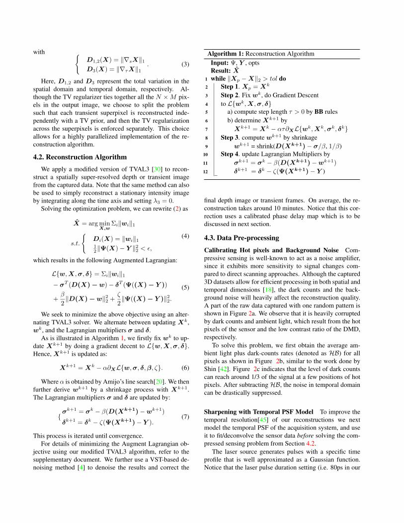
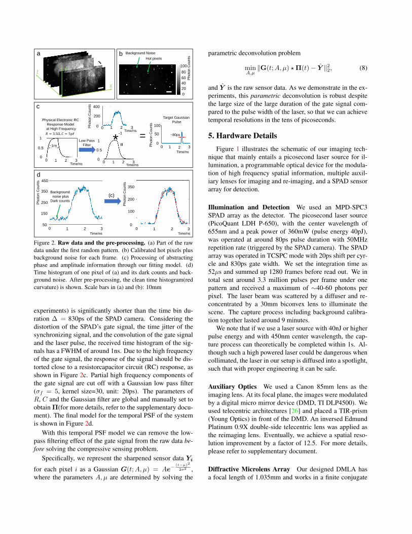
Calibrating Hot pixels and Background Noise Com-pressive sensing is well-known to act as a noise amplifier,since it exhibits more sensitivity to signal changes com-pared to direct scanning approaches. Although the captured3D datasets allow for efficient processing in both spatial andtemporal dimensions [18], the dark counts and the back-ground noise will heavily affect the reconstruction quality.A part of the raw data captured with one random pattern isshown in Figure 2a. We observe that it is heavily corruptedby dark counts and ambient light, which result from the hotpixels of the sensor and the low contrast ratio of the DMD,respectively.

To solve this problem, we first obtain the average am-bient light plus dark-counts rates (denoted as HB) for allpixels as shown in Figure 2b, similar to the work done byShin [42]. Figure 2c indicates that the level of dark countscan reach around 1/3 of the signal at a few positions of hotpixels. After subtractingHB, the noise in temporal domaincan be drastically suppressed.

Sharpening with Temporal PSF Model To improve thetemporal resolution[45] of our reconstructions we nextmodel the temporal PSF of the acquisition system, and useit to fit/deconvolve the sensor data before solving the com-pressed sensing problem from Section 4.2.

The laser source generates pulses with a specific timeprofile that is well approximated as a Gaussian function.Notice that the laser pulse duration setting (i.e. 80ps in our

𝑦𝑡

𝑥

0

20

40

60

80

100

Photo

n C

ounts

Background Noise

Hot pixels

a b

Background

noise plus

Dark counts

50

150

250

350

450

0 1 2 3

Photo

n C

ounts

Time/ns

d

0 1 2 30

100

200

350

Photo

n C

ounts

Time/ns

(c)

0 1 2 3Time/ns

200

400

0Photo

n C

ounts

0 1 2 3

Time/ns

50

100

0

Photo

n C

ounts

0 1 2 3

0.5

1

0

Time/ns Time/ns0 1 2 3

0.5

1

0

Low Pass

Filter

-1 =

Target Gaussian

PulsePhysical Electronic RC

Response Model

at High Frequency

~80ps

c

*𝑅 = 3.5Ω, 𝐶 = 5pF

~1ns 𝚷

Figure 2. Raw data and the pre-processing. (a) Part of the rawdata under the first random pattern. (b) Calibrated hot pixels plusbackground noise for each frame. (c) Processing of abstractingphase and amplitude information through our fitting model. (d)Time histogram of one pixel of (a) and its dark counts and back-ground noise. After pre-processing, the clean time histogram(redcurvature) is shown. Scale bars in (a) and (b): 10mm

experiments) is significantly shorter than the time bin du-ration ∆ = 830ps of the SPAD camera. Considering thedistortion of the SPAD’s gate signal, the time jitter of thesynchronizing signal, and the convolution of the gate signaland the laser pulse, the received time histogram of the sig-nals has a FWHM of around 1ns. Due to the high frequencyof the gate signal, the response of the signal should be dis-torted close to a resistorcapacitor circuit (RC) response, asshown in Figure 2c. Partial high frequency components ofthe gate signal are cut off with a Gaussian low pass filter(σf = 5, kernel size=30, unit: 20ps). The parameters ofR, C and the Gaussian filter are global and manually set toobtain Π(for more details, refer to the supplementary docu-ment). The final model for the temporal PSF of the systemis shown in Figure 2d.

With this temporal PSF model we can remove the low-pass filtering effect of the gate signal from the raw data be-fore solving the compressive sensing problem.

Specifically, we represent the sharpened sensor data Yi

for each pixel i as a Gaussian G(t;A,µ) = Ae−(t−µ)2

2σ2 ,where the parameters A,µ are determined by solving the

parametric deconvolution problem

minA,µ‖G(t;A,µ) ?Π(t)− Y ‖22, (8)

and Y is the raw sensor data. As we demonstrate in the ex-periments, this parametric deconvolution is robust despitethe large size of the large duration of the gate signal com-pared to the pulse width of the laser, so that we can achievetemporal resolutions in the tens of picoseconds.

5. Hardware DetailsFigure 1 illustrates the schematic of our imaging tech-

nique that mainly entails a picosecond laser source for il-lumination, a programmable optical device for the modula-tion of high frequency spatial information, multiple auxil-iary lenses for imaging and re-imaging, and a SPAD sensorarray for detection.

Illumination and Detection We used an MPD-SPC3SPAD array as the detector. The picosecond laser source(PicoQuant LDH P-650), with the center wavelength of655nm and a peak power of 360mW (pulse energy 40pJ),was operated at around 80ps pulse duration with 50MHzrepetition rate (triggered by the SPAD camera). The SPADarray was operated in TCSPC mode with 20ps shift per cyr-cle and 830ps gate width. We set the integration time as52µs and summed up 1280 frames before read out. We intotal sent around 3.3 million pulses per frame under onepattern and received a maximum of ∼40-60 photons perpixel. The laser beam was scattered by a diffuser and re-concentrated by a 30mm biconvex lens to illuminate thescene. The capture process including background calibra-tion together lasted around 9 minutes.

We note that if we use a laser source with 40nJ or higherpulse energy and with 450nm center wavelength, the cap-ture process can theoretically be completed within 1s. Al-though such a high powered laser could be dangerous whencollimated, the laser in our setup is diffused into a spotlight,such that with proper engineering it can be safe.

Auxiliary Optics We used a Canon 85mm lens as theimaging lens. At its focal plane, the images were modulatedby a digital micro mirror device (DMD, TI DLP4500). Weused telecentric architectures [26] and placed a TIR-prism(Young Optics) in front of the DMD. An inversed EdmundPlatinum 0.9X double-side telecentric lens was applied asthe reimaging lens. Eventually, we achieve a spatial reso-lution improvement by a factor of 12.5. For more details,please refer to supplementary document.

Diffractive Microlens Array Our designed DMLA hasa focal length of 1.035mm and works in a finite conjugate

0

50

100

150

200

250

300ps

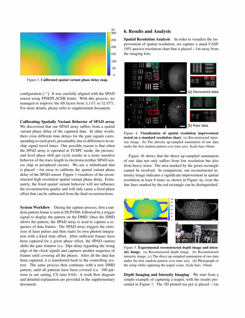
Figure 3. Calibrated spatial variant phase delay map.

configuration [27]. It was carefully aligned with the SPADsensor using FINEPLACER femto. With this process, wemanaged to improve the fill factor from 3.14% to 52.87%.For more details, please refer to supplemental document.

Calibrating Spatially Variant Behavior of SPAD arrayWe discovered that our SPAD array suffers from a spatialvariant phase delay of the captured data. In other words,there exist different time delays for the gate signals corre-sponding to each pixel, presumably due to differences in on-chip signal travel times. One possible reason is that whenthe SPAD array is operated at TCSPC mode, the picosec-ond level phase shift per cycle results in a more sensitivebehavior of the trace length in electronics(either SPAD sen-sor chip or peripheral circuit). We use a whiteboard thatis placed ∼1m away to calibrate the spatial variant phasedelay of the SPAD sensor. Figure 3 visualizes of the recon-structed high resolution spatial variant phase delay. Fortu-nately, the fixed spatial variant behavior will not influencethe reconstruction quality and will only cause a fixed phaseoffset that can be subtracted from the final reconstructions.

System Workflow During the capture process, first a ran-dom pattern frame is sent to DLP4500, followed by a triggersignal to display the pattern on the DMD. Once the DMDshows the pattern, the SPAD array is used to capture a se-quence of data frames. The SPAD array triggers the emis-sion of laser pulses and then starts its own photon integra-tion with a fixed time offset. After sufficient frames havebeen captured for a given phase offset, the SPAD camerashifts the gate window (i.e. 20ps delay regarding the risingedge of the clock signal) and captures another sequence offrames until covering all the phases. After all the data hasbeen captured, it is transferred back to the controlling sys-tem. The same process then continues with a new DMDpattern, until all patterns have been covered (i.e. 100 pat-terns in our setting, CS ratio 0.64). A work flow diagramand detailed explanation are provided in the supplementarydocument.

6. Results and AnalysisSpatial Resolution Analysis In order to visualize the im-provement of spatial resolution, we capture a stand UASF1951 passive resolution chart that is placed∼1m away fromthe imaging lens.

(a) Recovered data

(b) Raw data

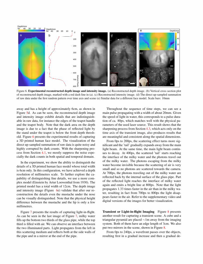
Figure 4. Visualization of spatial resolution improvementtested on a standard resolution chart. (a) Reconstructed inten-sity image. (b) The directly up-sampled summation of raw dataunder the first random pattern over time axis. Scale bars:10mm

Figure 4b shows that the direct up-sampled summationof raw data not only suffers from low resolution but alsofrom heavy noise. The area marked by the green rectanglecannot be resolved. In comparison, our reconstructed in-tensity image indicates a significant improvement in spatialresolution at least 8 times as shown in Figure 4a, even thefine lines marked by the red rectangle can be distinguished.

50

40

30

20

10

0

mma

b

c

d

Figure 5. Experimental reconstructed depth image and inten-sity image. (a) Reconstructed depth image. (b) Reconstructedintensity image. (c) The direct up-sampled summation of raw dataunder the first random pattern over time axis. (d) Photograph ofthe setup while capturing the teapot scene. Scale bars: 10mm

Depth Imaging and Intensity Imaging We start from asimple example of capturing a teapot, with the results pre-sented in Figure 5. The 3D printed tea pot is placed ∼1m

50 40 30 20 10 0Depth/mm

0

100

200

300

400

500

600

700

800

Mark

ed P

ixels

b

50 40 30 20 10 0Depth/mm

a c d

0

20

40

60 Depth/mme

e1

e2

e3

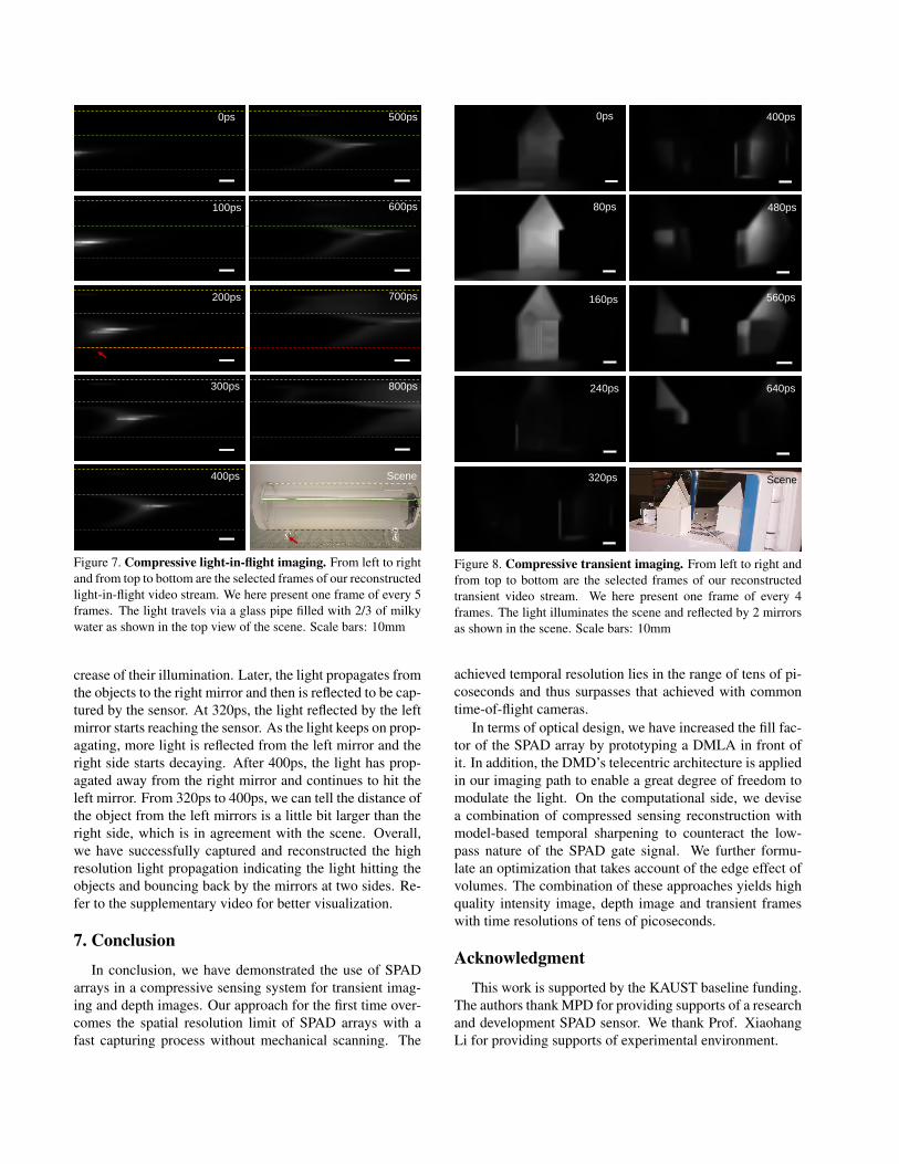
Figure 6. Experimental reconstructed depth image and intensity image. (a) Reconstructed depth image. (b) Vertical cross section plotof reconstructed depth image, marked with a red dash line in (a). (c) Reconstructed intensity image. (d) The direct up-sampled summationof raw data under the first random pattern over time axis and scene (e) Similar data for a different face model. Scale bars: 10mm

away and has a height of approximately 6cm, as shown inFigure 5d. As can be seen, the reconstructed depth imageand intensity image exhibit details that are indistinguish-able in raw data, for instance the edges of the teapot handleand the teapot body. Note that the dark area on the depthimage is due to a fact that the phase of reflected light bythe stand under the teapot is below the front depth thresh-old. Figure 6 presents the experimental results of capturinga 3D printed human face model. The visualization of thedirect up-sampled summation of raw data is quite noisy andhighly corrupted by dark counts. With the sharpening pro-cess from Section 4.1, we mostly suppress the noise espe-cially the dark counts in both spatial and temporal domain.

In the experiment, we show the ability to distinguish thedetails of a 3D printed human face model whose total widthis 6cm only. In this configuration, we have achieved a depthresolution of millimetres scale. To further explore the ca-pability of distinguishing fine details, we use a more com-plex model (Einstein by Artur Loewenthal from 1930). Theprinted model has a total width of 12cm. The depth imageand intensity image (Figure 6e) validate that after our re-construction the details even the mustache under the nosecan be visually distinguished. Note that the physical heightdifference between the mustache and the lip is only a fewmillimetres.

Figure 7 presents the results of capturing light-in-flight.As can be seen in the last image of Figure 7, milky waterfills up the bottom two thirds of the glass pipe, while the topthird is filled with air. We can observe an interface betweenthe two illuminated parts. Light propagates from the left inthis scattering medium and reflects both at the side walls ofthe pipe and in a mirror at the end of the pipe.

Throughout the sequence of time steps, we can see amain pulse propagating with a width of about 20mm. Giventhe speed of light in water, this corresponds to a pulse dura-tion of ca. 80ps, which matches well with the physical pa-rameters of the used laser source. This result shows that thesharpening process from Section 4.3, which acts only on thetime axis of the transient image, also produces results thatare meaningful and consistent along the spatial dimensions.

From 0ps to 200ps, the scattering effect turns more sig-nificant and the ’tail’ gradually expands away from the mainlight beam. At the same time, the main light beam contin-ues to decay. At 400ps, the scattered ’tail’ starts reachingthe interface of the milky water and the photons travel outof the milky water. The photons escaping from the milkywater become invisible because the scattering of air is verysmall and so no photons are scattered towards the camera.At 700ps, the photons traveling out of the milky water arereflected back by the internal surface of the glass pipe. Partof the reflected light reaches the interface of milky wateragain and emits a bright line at 800ps. Note that the lightpropagates 1.33 times faster in the air than in the milky wa-ter, resulting in fact from 700ps to 800ps the light disap-pears faster in the air. Refer to the supplementary video anddigital versions of the images for better visualization.

Transient or Light-in-flight Imaging Figure 8 presentsanother result for capturing a transient scene. A cube and atriangular pyramid are placed ∼1m away from the imagingsystem. Both of them have an edge length of 3cm. We alsoput two mirrors in the scene, shown in Figure 8.

From 0ps to 240ps, a wavefront passes over the objects,resulting first in a gradual increase and then a gradual de-

0ps

100ps

200ps

300ps

400ps

500ps

600ps

700ps

800ps

Scene

Figure 7. Compressive light-in-flight imaging. From left to rightand from top to bottom are the selected frames of our reconstructedlight-in-flight video stream. We here present one frame of every 5frames. The light travels via a glass pipe filled with 2/3 of milkywater as shown in the top view of the scene. Scale bars: 10mm

crease of their illumination. Later, the light propagates fromthe objects to the right mirror and then is reflected to be cap-tured by the sensor. At 320ps, the light reflected by the leftmirror starts reaching the sensor. As the light keeps on prop-agating, more light is reflected from the left mirror and theright side starts decaying. After 400ps, the light has prop-agated away from the right mirror and continues to hit theleft mirror. From 320ps to 400ps, we can tell the distance ofthe object from the left mirrors is a little bit larger than theright side, which is in agreement with the scene. Overall,we have successfully captured and reconstructed the highresolution light propagation indicating the light hitting theobjects and bouncing back by the mirrors at two sides. Re-fer to the supplementary video for better visualization.

7. Conclusion

In conclusion, we have demonstrated the use of SPADarrays in a compressive sensing system for transient imag-ing and depth images. Our approach for the first time over-comes the spatial resolution limit of SPAD arrays with afast capturing process without mechanical scanning. The

0ps

80ps

400ps

480ps

560ps160ps

240ps 640ps

320ps Scene

Figure 8. Compressive transient imaging. From left to right andfrom top to bottom are the selected frames of our reconstructedtransient video stream. We here present one frame of every 4frames. The light illuminates the scene and reflected by 2 mirrorsas shown in the scene. Scale bars: 10mm

achieved temporal resolution lies in the range of tens of pi-coseconds and thus surpasses that achieved with commontime-of-flight cameras.

In terms of optical design, we have increased the fill fac-tor of the SPAD array by prototyping a DMLA in front ofit. In addition, the DMD’s telecentric architecture is appliedin our imaging path to enable a great degree of freedom tomodulate the light. On the computational side, we devisea combination of compressed sensing reconstruction withmodel-based temporal sharpening to counteract the low-pass nature of the SPAD gate signal. We further formu-late an optimization that takes account of the edge effect ofvolumes. The combination of these approaches yields highquality intensity image, depth image and transient frameswith time resolutions of tens of picoseconds.

Acknowledgment

This work is supported by the KAUST baseline funding.The authors thank MPD for providing supports of a researchand development SPAD sensor. We thank Prof. XiaohangLi for providing supports of experimental environment.

References[1] N. Abramson. Light-in-flight recording by holography. Op-

tics Letters, 3(4):121–123, Oct 1978. 1, 2[2] N. Abramson. Light-in-flight recording: high-speed holo-

graphic motion pictures of ultrafast phenomena. Applied op-tics, 22(2):215–232, 1983. 2

[3] N. H. Abramson and K. G. Spears. Single pulse light-in-flight recording by holography. Applied optics, 28(10):1834–1841, 1989. 2

[4] L. Azzari and A. Foi. Variance stabilization fornoisy+estimate combination in iterative poisson denoising.IEEE Signal Processing Letters, 23(8):1086–1090, Aug2016. 4

[5] R. G. Baraniuk. Compressive sensing. IEEE Signal Process-ing Magazine, 24(4), 2007. 3

[6] E. J. Candes, J. K. Romberg, and T. Tao. Stable signal recov-ery from incomplete and inaccurate measurements. Comm.Pure Appl. Math, 59(8):1207–1223, 2006. 2

[7] H. Chen, M. S. Asif, A. C. Sankaranarayanan, and A. Veer-araghavan. Fpa-cs: Focal plane array-based compressiveimaging in short-wave infrared. In Proc. CVPR, pages 2358–2366. IEEE, 2015. 3

[8] J. F. Claerbout and F. Muir. Robust modeling with erraticdata. Geophysics, 38(5):826–844, 1973. 2

[9] W. Dai and O. Milenkovic. Subspace pursuit for compressivesensing signal reconstruction. IEEE Transactions on Infor-mation Theory, 55(5):2230–2249, 2009. 3

[10] D. L. Donoho. Compressed sensing. IEEE Transactions oninformation theory, 52(4):1289–1306, 2006. 2

[11] D. L. Donoho and M. Elad. Optimally sparse represen-tation in general (nonorthogonal) dictionaries via l1 mini-mization. Proceedings of the National Academy of Sciences,100(5):2197–2202, 2003. 3

[12] D. L. Donoho and X. Huo. Uncertainty principles and idealatomic decomposition. IEEE Transactions on InformationTheory, 47(7):2845–2862, 2001. 3

[13] D. L. Donoho and P. B. Stark. Uncertainty principles andsignal recovery. SIAM Journal on Applied Mathematics,49(3):906–931, 1989. 3

[14] A. Dorrington, J. Godbaz, M. Cree, A. Payne, andL. Streeter. Separating true range measurements from multi-path and scattering interference in commercial range cam-eras. In Proc. Electronic Imaging, 2011. 1

[15] M. F. Duarte, M. A. Davenport, D. Takbar, J. N. Laska,T. Sun, K. F. Kelly, and R. G. Baraniuk. Single-pixel imag-ing via compressive sampling. IEEE Signal Processing Mag-azine, 25(2):83–91, 2008. 3

[16] J. H. Ender. On compressive sensing applied to radar. SignalProcessing, 90(5):1402–1414, 2010. 3

[17] G. Gariepy, N. Krstajic, R. Henderson, C. Li, R. R. Thomson,G. S. Buller, B. Heshmat, R. Raskar, J. Leach, and D. Fac-cio. Single-photon sensitive light-in-fight imaging. NatureCommunications, 6, 2015. 2

[18] G. Gariepy, F. Tonolini, R. Henderson, J. Leach, and D. Fac-cio. Detection and tracking of moving objects hidden fromview. Nature Photonics, 10(1):23–26, 2016. 2, 4

[19] E. D. Gluskin. Norms of random matrices and widths offinite-dimensional sets. Mathematics of the USSR-Sbornik,48(1):173, 1984. 2

[20] L. Grippo, F. Lampariello, and S. Lucidi. A nonmonotoneline search technique for newtons method. SIAM Journal onNumerical Analysis, 23(4):707–716, 1986. 4

[21] O. Gupta, T. Willwacher, A. Velten, A. Veeraraghavan, andR. Raskar. Reconstruction of hidden 3d shapes using diffusereflections. Optics Express, 20(17):19096–19108, 2012. 1, 2

[22] F. Heide, W. Heidrich, M. Hullin, and G. Wetzstein. Dopplertime-of-flight imaging. ACM Trans. Graph. (SIGGRAPH),34(4):36, 2015. 2

[23] F. Heide, M. B. Hullin, J. Gregson, and W. Heidrich. Low-budget transient imaging using photonic mixer devices. ACMTrans. Graph. (SIGGRAPH), 32(4):45, 2013. 1, 2

[24] F. Heide, L. Xiao, W. Heidrich, and M. t. B. Hullin. Dif-fuse mirrors: 3D reconstruction from diffuse indirect illu-mination using inexpensive time-of-flight sensors. In Proc.CVPR, June 2014. 1

[25] F. Heide, L. Xiao, A. Kolb, M. B. Hullin, and W. Hei-drich. Imaging in scattering media using correlation imagesensors and sparse convolutional coding. Optics Express,22(21):26338–26350, 2014. 1

[26] T. Instruments. Dlp system optics application note, 2015. 5[27] G. Intermite, A. McCarthy, R. E. Warburton, X. Ren, F. Villa,

R. Lussana, A. J. Waddie, M. R. Taghizadeh, A. Tosi,F. Zappa, et al. Fill-factor improvement of si cmos single-photon avalanche diode detector arrays by integration ofdiffractive microlens arrays. Optics Express, 23(26):33777–33791, 2015. 6

[28] A. Kadambi, R. Whyte, A. Bhandari, L. Streeter, C. Barsi,A. Dorrington, and R. Raskar. Coded time of flight cameras:sparse deconvolution to address multipath interference andrecover time profiles. ACM Transactions on Graphics (ToG),32(6):167, 2013. 2

[29] B. S. Kashin. Diameters of some finite-dimensional sets andclasses of smooth functions. Izvestiya Rossiiskoi AkademiiNauk. Seriya Matematicheskaya, 41(2):334–351, 1977. 2

[30] C. Li, W. Yin, and Y. Zhang. Users guide for tval3: Tv min-imization by augmented lagrangian and alternating directionalgorithms. CAAM report, 20:46–47, 2009. 4

[31] D.-U. Li, J. Arlt, J. Richardson, R. Walker, A. Buts,D. Stoppa, E. Charbon, and R. Henderson. Real-time flu-orescence lifetime imaging system with a 32× 32 0.13 µmcmos low dark-count single-photon avalanche diode array.Optics Express, 18(10):10257–10269, 2010. 2

[32] F. Li, A. P. Huaijin Chen, C. Yeh, K. He, A. Veeraragha-van, and O. Cossairt. Cs-tof: High-resolution compres-sive time-of-flight imaging. Optics Express, 25(25):31096–31110, 2017. 2

[33] J. Lin, Y. Liu, J. Suo, and Q. Dai. Frequency-domain tran-sient imaging. IEEE transactions on pattern analysis andmachine intelligence, 39(5):937–950, 2017. 2

[34] N. Naik, S. Zhao, A. Velten, R. Raskar, and K. Bala. Sin-gle view reflectance capture using multiplexed scattering andtime-of-flight imaging. ACM Trans. Graph. (SIGGRAPHAsia), 30(6):171:1–171:10, 2011. 1

[35] D. O’Connor. Time-correlated single photon counting. Aca-demic Press, 2012. 2

[36] G. Oliveri, N. Anselmi, and A. Massa. Compressive sens-ing imaging of non-sparse 2d scatterers by a total-variationapproach within the born approximation. IEEE Transactionson Antennas and Propagation, 62(10):5157–5170, 2014. 3

[37] M. O’Toole, F. Heide, D. B. Lindell, K. Zang, S. Diamond,and G. Wetzstein. Reconstructing transient images fromsingle-photon sensors. In Proc. IEEE CVPR, pages 2289–2297, 2017. 2

[38] A. Payne, A. Daniel, A. Mehta, B. Thompson, C. S. Bamji,D. Snow, H. Oshima, L. Prather, M. Fenton, L. Kordus,et al. 7.6 a 512× 424 cmos 3d time-of-flight image sensorwith multi-frequency photo-demodulation up to 130mhz and2gs/s adc. In Proc. ISSCC, pages 134–135. IEEE, 2014. 1

[39] J. Richardson, R. Walker, L. Grant, D. Stoppa, F. Borghetti,E. Charbon, M. Gersbach, and R. K. Henderson. A 32×32 50ps resolution 10 bit time to digital converter array in130nm cmos for time correlated imaging. In Proc. CICC,pages 77–80. IEEE, 2009. 2

[40] F. Santosa and W. W. Symes. Linear inversion of band-limited reflection seismograms. SIAM Journal on Scientificand Statistical Computing, 7(4):1307–1330, 1986. 2

[41] R. Schwarte, Z. Xu, H. Heinol, J. Olk, R. Klein,B. Buxbaum, H. Fischer, and J. Schulte. New electro-opticalmixing and correlating sensor: facilities and applications ofthe photonic mixer device. In Proc. SPIE, volume 3100,pages 245–253, 1997. 1

[42] D. Shin, F. Xu, D. Venkatraman, R. Lussana, F. Villa,F. Zappa, V. K. Goyal, F. N. Wong, and J. H. Shapiro.Photon-efficient imaging with a single-photon camera. Na-ture Communications, 7, 2016. 2, 4

[43] S. Su, F. Heide, R. Swanson, J. Klein, C. Callenberg,M. Hullin, and W. Heidrich. Material classification using rawtime-of-flight measurements. In Proc. CVPR, pages 3503–3511, 2016. 2

[44] S. Surti. Update on time-of-flight pet imaging. Journal ofNuclear Medicine, 56(1):98–105, 2015. 2

[45] R. Tadano, A. K. Pediredla, K. Mitra, and A. Veeraraghavan.Spatial phase-sweep: Increasing temporal resolution of tran-sient imaging using a light source array. In Proc. ICIP, pages1564–1568. IEEE, 2016. 4

[46] A. Velten, T. Willwacher, O. Gupta, A. Veeraraghavan, M. G.Bawendi, and R. Raskar. Recovering three-dimensionalshape around a corner using ultrafast time-of-flight imaging.Nature Communications, 3:745, 2012. 1, 2

[47] A. Velten, D. Wu, A. Jarabo, B. Masia, C. Barsi, C. Joshi,E. Lawson, M. Bawendi, D. Gutierrez, and R. Raskar.Femto-photography: capturing and visualizing the propaga-tion of light. ACM Trans. Graph. (SIGGRAPH), 32(4):44,2013. 1, 2

[48] X. Yuan, P. Llull, X. Liao, J. Yang, D. J. Brady, G. Sapiro,and L. Carin. Low-cost compressive sensing for color videoand depth. In Proc. CVPR, pages 3318–3325, 2014. 3