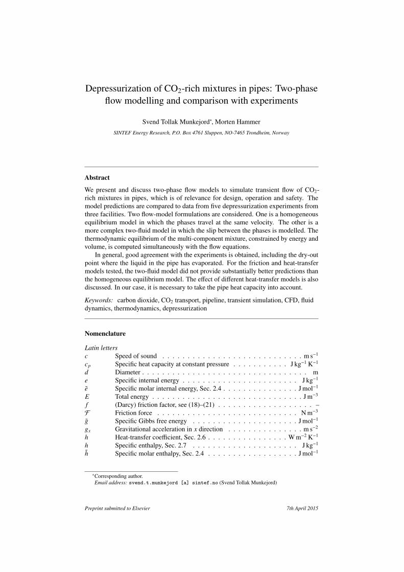
Depressurization of CO2-rich mixtures in pipes: Two-phaseflow modelling and comparison with experiments

Svend Tollak Munkejord∗, Morten Hammer

SINTEF Energy Research, P.O. Box 4761 Sluppen, NO-7465 Trondheim, Norway

Abstract

We present and discuss two-phase flow models to simulate transient flow of CO2-rich mixtures in pipes, which is of relevance for design, operation and safety. Themodel predictions are compared to data from five depressurization experiments fromthree facilities. Two flow-model formulations are considered. One is a homogeneousequilibrium model in which the phases travel at the same velocity. The other is amore complex two-fluid model in which the slip between the phases is modelled. Thethermodynamic equilibrium of the multi-component mixture, constrained by energy andvolume, is computed simultaneously with the flow equations.

In general, good agreement with the experiments is obtained, including the dry-outpoint where the liquid in the pipe has evaporated. For the friction and heat-transfermodels tested, the two-fluid model did not provide substantially better predictions thanthe homogeneous equilibrium model. The effect of different heat-transfer models is alsodiscussed. In our case, it is necessary to take the pipe heat capacity into account.

Keywords: carbon dioxide, CO2 transport, pipeline, transient simulation, CFD, fluiddynamics, thermodynamics, depressurization

Nomenclature

Latin lettersc Speed of sound . . . . . . . . . . . . . . . . . . . . . . . . . . . . m s−1

cp Specific heat capacity at constant pressure . . . . . . . . . . . J kg−1 K−1

d Diameter . . . . . . . . . . . . . . . . . . . . . . . . . . . . . . . . . me Specific internal energy . . . . . . . . . . . . . . . . . . . . . . . J kg−1

e Specific molar internal energy, Sec. 2.4 . . . . . . . . . . . . . . . J mol−1

E Total energy . . . . . . . . . . . . . . . . . . . . . . . . . . . . . . J m−3

f (Darcy) friction factor, see (18)–(21) . . . . . . . . . . . . . . . . . . . –F Friction force . . . . . . . . . . . . . . . . . . . . . . . . . . . . N m−3

g Specific Gibbs free energy . . . . . . . . . . . . . . . . . . . . . J mol−1

gx Gravitational acceleration in x direction . . . . . . . . . . . . . . . m s−2

h Heat-transfer coefficient, Sec. 2.6 . . . . . . . . . . . . . . . . W m−2 K−1

h Specific enthalpy, Sec. 2.7 . . . . . . . . . . . . . . . . . . . . . J kg−1

h Specific molar enthalpy, Sec. 2.4 . . . . . . . . . . . . . . . . . . J mol−1

∗Corresponding author.Email address: svend.t.munkejord [a] sintef.no (Svend Tollak Munkejord)

Preprint submitted to Elsevier 7th April 2015

m Mass flux . . . . . . . . . . . . . . . . . . . . . . . . . . . . kg m−2 s−1

n Time step . . . . . . . . . . . . . . . . . . . . . . . . . . . . . . . . . –n Composition vector . . . . . . . . . . . . . . . . . . . . . . . mol mol−1

Nu Nusselt number . . . . . . . . . . . . . . . . . . . . . . . . . . . . . . –P Pressure . . . . . . . . . . . . . . . . . . . . . . . . . . . . . . . . . PaPr Prandtl number . . . . . . . . . . . . . . . . . . . . . . . . . . . . . . –q Heat flux . . . . . . . . . . . . . . . . . . . . . . . . . . . . . . . W m−2

Q Heat . . . . . . . . . . . . . . . . . . . . . . . . . . . . . . . . . W m−3

r Radius . . . . . . . . . . . . . . . . . . . . . . . . . . . . . . . . . . mR Universal gas constant . . . . . . . . . . . . . . . . . . . . J mol−1 K−1

Re Reynolds number . . . . . . . . . . . . . . . . . . . . . . . . . . . . . –s Specific molar entropy, Sec. 2.4 . . . . . . . . . . . . . . . . J mol−1 K−1

t Time . . . . . . . . . . . . . . . . . . . . . . . . . . . . . . . . . . . . sT Temperature . . . . . . . . . . . . . . . . . . . . . . . . . . . . . . . . Ku Velocity . . . . . . . . . . . . . . . . . . . . . . . . . . . . . . . . m s−1

v Specific molar volume, Sec. 2.4 . . . . . . . . . . . . . . . . . . m3 mol−1

W State function . . . . . . . . . . . . . . . . . . . . . . . . . . . . J mol−1

x Spatial coordinate . . . . . . . . . . . . . . . . . . . . . . . . . . . . mz Mass fraction . . . . . . . . . . . . . . . . . . . . . . . . . . . . kg kg−1

Z Compressibility factor . . . . . . . . . . . . . . . . . . . . . . . . . . . –

Greek lettersα Volume fraction . . . . . . . . . . . . . . . . . . . . . . . . . . . m3 m−3

δ Factor in (12) . . . . . . . . . . . . . . . . . . . . . . . . . . . . . . . –λ Thermal conductivity . . . . . . . . . . . . . . . . . . . . . . W m−1 K−1

µ Dynamic viscosity . . . . . . . . . . . . . . . . . . . . . . . . kg m−1 s−1

Ψ Mass-transfer, see (10) . . . . . . . . . . . . . . . . . . . . . kg m−3 s−1

φi Interfacial momentum exchange . . . . . . . . . . . . . . . . . . N m−3

Φ Coefficient in (18) . . . . . . . . . . . . . . . . . . . . . . . . . . . . . –ρ (Mass) density . . . . . . . . . . . . . . . . . . . . . . . . . . . . kg m−3

Subscriptsamb Ambient conditionB Bernoulli, Sec. 2.7c Chokef Fluidg Gasi Interfacial or inner or initialj Componentk Phase k` Liquidmin Minimumo OuterR Riemann, Sec. 2.7spec Specified conditionw Wall

AbbreviationsBBC Bernoulli-choking-pressure boundary condition, Sec. 2.7BC Boundary conditionC ColburnCBC Characteristic-based boundary condition, Sec. 2.7

2

CCS CO2 capture & storageCFL Courant–Friedrichs–LewyEOS Equation of stateFORCE First-order centredGERG Groupe européen de recherches gazièresGW Gungor–WintertonHEM Homogeneous equilibrium modelMUSTA Multistage centredPR Peng–RobinsonTFM Two-fluid model

1. Introduction

Large-scale deployment of CCS (CO2 capture & storage) will require transportof large quantities of CO2 from the points of capture to the storage sites. A majorpart will probably be handled in pipeline networks. CO2 transport by pipeline differsfrom e.g. that of natural gas in a number of ways. First, the CO2 will normally be ina liquid or dense liquid state, while the natural gas most often is in a dense gaseousstate, see e.g. Aursand et al. (2013). Next, depending on the capture technology, theCO2 will contain various impurities (NETL, 2013), which may, even in small quantities,significantly affect the thermophysical properties (Li et al., 2011a,b), which, in turn,affect the depressurization and flow behaviour (Munkejord et al., 2010).

Although CO2 has been transported by pipeline for the purpose of enhanced oilrecovery (US DOE, 2010), mainly in the USA, the CCS case will likely be different, dueto the different impurities, and due to the proximity, in many cases, to densely populatedareas. As a result of this, and because of the expected scale of CCS (IEA, 2014), it willbe of importance to design and operate CO2 pipelines in an economical and safe way.

It has been found that a pipeline transporting CO2 will be more susceptible torunning-ductile fracture than one carrying natural gas (Mahgerefteh et al., 2012; Aursandet al., 2014). One part of the design to avoid running-ductile fracture necessitatesaccurate models predicting the depressurization behaviour of the relevant CO2-richmixtures, noting that existing semi-empirical models have been deemed not to be directlyapplicable to CO2 pipelines (Jones et al., 2013). In this respect, the development ofcoupled fluid-structure models containing more physics (Aihara and Misawa, 2010;Mahgerefteh et al., 2012; Nordhagen et al., 2012) may lead to a better predictivecapability. Furthermore, even though the CO2 pipeline is primarily designed to operatein the single-phase region, two-phase flow may occur. This may be due to fluctuatingCO2 supply (Klinkby et al., 2011) or during transient events, such as start-up, shut-in ordepressurization (Munkejord et al., 2013; Hetland et al., 2014). During depressurization,low temperatures may be attained. It is of interest to have good estimates of thesetemperatures, since pipeline materials have a minimum temperature at which they losetoughness.

The computation of near-field dispersion of CO2 from a leaking pipeline forms partof quantified risk analysis and entails the 2D or 3D modelling of the expanding CO2jet, see e.g. Wareing et al. (2014). However, such computations require a description ofthe CO2 state at the puncture or rupture of the pipe. One suitable way to do this is toemploy a pipe-flow model.

The above issues call for the development of engineering tools accurately predictingthe single- and two-phase flow of CO2-rich mixtures in pipes. The present work

3

represents one step in this direction. The published literature containing relevant CO2-flow data has been scarce, but recently, some depressurization experiments with pureCO2 and with CO2-rich mixtures have been published. Depressurization experiments areinteresting for two reasons. First, the pressure-wave propagation during depressurizationis interesting in itself, due to its application to fracture-propagation control. Second, theflow-model formulation has inherent wave-propagation velocities, which ought to agreewith the experimental observations. This may be challenging in the two-phase region.

Drescher et al. (2014) presented experiments and simulations for depressurizationof three CO2-N2 mixtures. The N2 content in the three experiments was 10, 20 and30 mol %. The initial conditions for the experiments were approximately 12.0 MPaand 20 ◦C for all cases. The tube used was about 140 m long and the internal diameterwas 10.0 mm. The logging rate of the pressure was 5 kHz for the initial 10 s, thereafter100 Hz. Simulations were performed using a homogeneous equilibrium model (HEM),and good agreement with the experiments was obtained for the pressure. Comparisonbetween simulated and measured temperature indicated, among other things, slowtemperature sensors.

Botros et al. (2013) presented an experiment with a mixture of 72.6 mol % CO2and 27.4 mol % CH4, representing gas used for enhanced oil recovery. A specializedhigh-pressure shock tube (42 m long, and 38.1 mm internal diameter) was used. Theinner pipe wall was honed to get a smooth surface, with very little friction, to betterresemble larger industrial pipes. The experiment was conducted with a very highinitial pressure of 28.568 MPa, and a high initial temperature of 40.5 ◦C. Botros et al.employed high-frequency response dynamic-pressure transducers, with a logging rateup to 20 kHz. The shock-tubes and experiments were designed to measure and studythe decompression wave speed, the velocity of the rarefaction wave propagating into thepipeline, after rupture of a burst disc.

National Grid (Cosham et al., 2012) have conducted 14 shock-tube experiments fromdense/liquid phase pure CO2 and CO2-rich mixtures with impurities (H2, N2, O2, CH4).The pipeline segment used was 144 m long and had an internal diameter of 146.36 mm.One of the mixture experiments, CO2-H2-N2-O2-CH4, was presented in more detail,and the pressure levels for the initial 50 ms were plotted. Pressure was sampled at afrequency of 100 kHz. The motivation for performing the shock-tube experiments wasto improve the understanding of CO2 and CO2-mixture decompression behaviour, inorder to the predict the pipe material toughness required to arrest a running-ductilefracture. The initial conditions ranged from 3.89 MPa to 15.4 MPa and from 0.1 ◦C to35.6 ◦C.

The CO2-H2-N2-O2-CH4 experiment of Cosham et al. (2012), and the Botros et al.(2013) experiment, were compared to numerical simulations by Elshahomi et al. (2015).They used a finite-volume approach in ANSYS Fluent, and discretization of the pipein 2D axial symmetry. The Advection Upstream Splitting Method of Liou and Steffen(1993) was employed for the inter-cell flux calculations. For the thermodynamic closure,Elshahomi et al. used the GERG-2008 equation of state (EOS) (Kunz and Wagner,2012).

Data from Cosham et al. (2012), including the CO2-H2-N2-O2-CH4 experiment,were also considered by Jie et al. (2012), who employed a semi-implicit numericalmethod to solve the HEM (Xu et al., 2014) with the Peng–Robinson–Stryjek–Vera EOS(Stryjek and Vera, 1986).

For the case of pure CO2, Brown et al. (2014) compared a homogeneous equilibriummodel and a two-fluid model (TFM) with a formulation similar to that of Paillère et al.(2003), to depressurization experiments. Both chemical potential and temperature were

4

relaxed, while the pressure of the two phases was identical. The experiments wereconducted in a straight 260 m long pipe with an internal diameter of 233 mm. Betteragreement between the experiments and the TFM was observed, than for the HEM.

In this work, we consider multicomponent CO2 mixtures and discuss two formula-tions of the flow model. The first is a HEM while the second is a TFM. We discuss theperformance of the models comparing with data from five different full-bore pressure-release experiment from three different facilities (Botros et al., 2013; Cosham et al.,2012; Drescher et al., 2014). The data from the two first facilities are pressure datafrom the first part of the depressurization. The data from the latter facility are pressureand temperature data taken over a longer time span, such that wall friction, interphasicfriction and heat transfer are expected to play a significant role. In particular, the dataand simulations include the dry-out point, i.e., the point at which all the liquid hasevaporated. Dry-out is challenging to model, since it is sensitive to both the flow-modelformulation and the employed closure relations.

In our compressible two-phase flow models, full thermodynamic equilibrium (pres-sure, temperature and chemical potential) is assumed. With this assumption, the iso-choric–iso-energetic phase-equilibrium problem must be solved, unless modellingsimplifications are made. When engineering equations of state are required, this isa challenging and CPU-demanding problem. As a consequence, computational fluiddynamics (CFD) simulations with advanced EOSs are commonly performed using tabu-lated thermodynamic state variables and fluid phase properties (Elshahomi et al., 2015;Pini et al., 2015; Swesty, 1996; Timmes and Swesty, 2000; Xia et al., 2007; Kunicket al., 2008). Thermodynamic consistency of the tabulated approximation is rarelyaddressed, even though this might lead to some entropy production (Swesty, 1996).For single-component fluids, there are some examples of finite-volume simulationswhere engineering EOSs are solved directly, without tabulation prior to the simula-tion (Giljarhus et al., 2012; Hammer et al., 2013; Hammer and Morin, 2014; Brownet al., 2014). Michelsen (1999) describes a framework for solving the multi-componentiso-choric–iso-energetic phase equilibrium that guarantees a solution. In this work,the methods of Michelsen have been adapted and used for the Peng and Robinson(1976) (PR) EOS. For more CPU-demanding EOSs, like the multi-component referenceEOS GERG-2008 (Kunz and Wagner, 2012) or EOS-CG (Gernert and Span, 2010),practical implementations are likely required to use property tabulation. EOS-CG issimilar to GERG-2008, but the component interaction parameters are tuned to matchthe properties of CO2-rich systems. Different Helmholtz mixture rules are also used forsome components. EOS-CG is under development, and currently, only a limited set ofimpurities are supported.

The rest of this article is organized as follows: Section 2 briefly presents the formu-lation of the homogeneous equilibrium model and the two-fluid model, the employedmodels for thermophysical properties, as well as the constitutive models for frictionand heat transfer. Model predictions are compared to experiments and discussed inSection 3. Conclusions are drawn in Section 4.

2. Models

In this work, we model the pipeflow as one-dimensional. The flow can be single-phase or two-phase gas-liquid. The gas and the liquid consist of multiple chemicalcomponents. Gravity, friction and heat transfer to the surroundings are accounted forby source terms. Viscous effects other than wall or interphasic friction are ignored.Full thermodynamical equilibrium is assumed, i.e., the phases have the same pressure,

5

temperature and chemical potential. We consider two flow models, described in thefollowing. The first is a drift-flux model with no slip, or a homogeneous equilibriummodel. The second is a more complex two-fluid model, in which the interphasic frictionis explicitly modelled. For a mathematical background of two-phase flow modelling,see e.g. Drew (1983).

2.1. Homogeneous equilibrium model

In the homogeneous equilibrium model (HEM), it is assumed that the phases travelwith the same velocity. The governing equations will then have the same form as theEuler equations for single-phase compressible inviscid flow, and consist of a mass-conservation equation,

∂

∂t(ρ) +

∂

∂x(ρu) = 0, (1)

a momentum-balance equation,

∂

∂t(ρu) +

∂

∂x(ρu2 + P) = ρgx − Fw, (2)

and a balance equation for the total energy,

∂

∂t(E) +

∂

∂xu(E + P) = ρgxu + Q. (3)

Herein, ρ = αgρg + α`ρ` is the density of the gas (g) and liquid (`) mixture. u is thecommon velocity and P is the pressure. E = ρ(e + 1/2u2) is the total energy of themixture, while e =

(egαgρg + e`α`ρ`

)/ρ is the mixture specific internal energy. αk

denotes the volume fraction of phase k ∈ g, `. Fw is the wall friction and Q is theheat transferred through the pipe wall. gx is the gravitational acceleration in the axialdirection of the pipe.

2.2. Two-fluid model

In the two-fluid model (TFM), the phases may travel with different velocities. As aresult of this, the chemical composition may change along the pipe. We therefore solvea mass-conservation equation for each chemical component in the gas, as well as in theliquid:

∂

∂t(αgρgzg, j) +

∂

∂x(αgρgzg, jug) = Ψg, j, (4)

∂

∂t(α`ρ`z`, j) +

∂

∂x(α`ρ`z`, ju`) = Ψ`, j. (5)

The model further consists of a momentum-balance equation for each phase,

∂

∂t(αgρgug) +

∂

∂x(αgρgu2

g)

+ αg∂P∂x

+ φi = uiΨ + αgρggx − Fwg, (6)

∂

∂t(α`ρ`u`) +

∂

∂x(α`ρ`u2

`

)+ α`

∂P∂x− φi = −uiΨ + α`ρ`gx − Fw`, (7)

and a total-energy-balance equation for the gas-liquid mixture,

∂

∂t(Eg + E`) +

∂

∂x(Egug + αgugP) +

∂

∂x(E`u` + α`u`P) = αgρggxug + α`ρ`gxu`. (8)

6

Herein, Ek = ρk(ek + 1/2u2k) is the total energy of phase k. ui = 1/2

(ug + u`

)is the

interfacial momentum velocity. Morin and Flåtten (2012) showed that this choice ofinterfacial momentum velocity does not produce entropy, and Hammer and Morin (2014)further showed that it preserves the kinetic energy for the system. The volume fractionssatisfy

αg + α` = 1. (9)

Ψk, j is the mass transfer to chemical component j in phase k. Since mass is conserved,we have

Ψ =∑

j

Ψg, j = −∑

j

Ψ`, j. (10)

The mass transfer is calculated at each time step using an instantaneous relaxationprocedure analogous to the one described by Hammer and Morin (2014), imposing fullthermodynamic (pressure, temperature and chemical potential) equilibrium. This impliesthat the conserved mass of gas and liquid must be updated after the relaxation procedure.The characteristic wave-structure of the model (4)–(8) will, due to the instantaneousrelaxation, recover the structure of a model with a single mass-conservation equationper component.

φi denotes the interfacial momentum exchange. Here we employ the model

φi = ∆Pi∂αg

∂x+ Fi, (11)

where ∆Pi is the difference between the average bulk pressure and the average interfacialpressure. Fi is an interface friction model treated as a source term. Following earlierworks (Stuhmiller, 1977; Bestion, 1990; Munkejord et al., 2009), we take

∆Pi = δαgα`ρgρ`

αgρ` + α`ρg(ug − u`)2, (12)

where δ = 1.2.

2.3. Thermophysical property modelsIn order to model gas-liquid phase equilibrium, phase densities and energies, we

employ the Peng and Robinson (1976) EOS. Classical van der Waals mixing rulesand symmetric binary interaction parameters are used. For the ideal heat capacity,correlations from the American Petroleum Institute, research project 44 (1976) are used.The fluid thermal conductivity and dynamic viscosity are calculated using the TRAPPmodel (Ely and Hanley, 1981, 1983).

2.4. Phase equilibriumFor a numerical flow simulation, phase equilibrium must typically be determined

from the given amounts of the components, n, and additionally two state variables.Depending on the available input we employ one of three methods, listed with increasingcomplexity of the problem formulation:

• Initial conditions: Pressure (P) and temperature (T ) are specified (PT -flash)

• Boundary conditions: Pressure (P) and entropy (s) are specified (Ps-flash)

• Conserved variables: Specific molar internal energy (e) and specific molar volume(v) are specified (ev-flash)

7

The most common phase-equilibrium calculation, the PT -flash, is a global minimiz-ation problem for the Gibbs free energy, g, of the system. The difficulty in solving thisminimization lies in correctly to determine the number of phases and their composition.For the pressure and temperature range of the mixtures used in this work, it is knownthat the mixture can only exhibit a single-phase or a two phase, gas-liquid mixture,behaviour. This simplifies the minimization considerably. The two-phase PT -flash isthoroughly studied, and a numerical framework is described in detail by Michelsen andMollerup (2007).

In the single-phase pressure-temperature region where the equation of state, P =

P(T, v, n), only has one density root, it is not possible to distinguish between a gasphase and a liquid phase. In this case, the phase is defined to be liquid, when thecompressibility factor, Z = Pv/(RT ), is less than the pseudo-critical compressibilityfactor of the mixture (0.3074. . . for the Peng-Robinson EOS). Otherwise the phase isdefined to be gas. R is the universal gas constant.

The Ps-flash is a global minimization of enthalpy, h, subject to specifications onpressure, Pspec, entropy, sspec, and composition. For multicomponent mixtures, thePs-flash can be transformed to a single-variable unconstrained minimization problemutilizing a state function, W, and the PT -flash in an inner loop (Michelsen, 1999):

W (T ) = −gmin − T sspec. (13)

Here the result of the PT -flash Gibbs free energy minimization is gmin. Differentiating(13) with respect to T , we obtain

dWdT

= smin − sspec (14)

where smin is the entropy evaluated at the Gibbs free energy minimum found by thePT -flash. This shows that the entropy constraint is satisfied at the stationary point ofthe minimization.

The ev-flash, or iso-choric–iso-energetic phase equilibrium problem, is a globalminimization of entropy with constraints on internal energy, espec, specific volume, vspec,and composition. In a similar manner, a state function can be used to transform theconstrained minimization to an unconstrained problem,

W (T, P) = −

(gmin − espec − Pvspec

)T

. (15)

Again the stationary point found by differentiating (15) satisfies the constraints oninternal energy and specific volume,

∂W∂T

=

(hmin − espec − Pvspec

)T 2 , (16)

∂W∂P

= −

(vmin − vspec

)T

, (17)

where hmin is the enthalpy evaluated at the Gibbs free energy minimum found by thePT -flash.

In order to get a properly scaled Hessian matrix, ln T and ln P are used as variablesinstead of T and P. This nested-loop approach is CPU demanding compared to solvingthe full set of equilibrium conditions simultaneously, but guarantees convergence. At thesame time, good initial values are available from the previous time step. The approachfor solving the full equilibrium equation set described by Michelsen (1999) is used inthis work, and the nested-loop approach is used as a fail-safe alternative.

8

2.5. Friction modelsThe wall friction for the homogeneous equilibrium model is calculated as

Fw =

fk

m|m|2ρkdi

for single-phase flow

f`m|m|2ρ`di

Φ for two-phase flow,(18)

where fk = f (Rek) is the Darcy friction factor, Rek = |m|di/µk is the Reynolds numberfor phase k and m = ρu is the mass flux. The coefficient Φ is an empirical correlation,which is used to account for two-phase flow, and depends on various properties of bothphases. Here we have employed the Friedel (1979) correlation. Details of the calculationof the two-phase coefficient Φ, and also further discussion, can be found in Aakenes(2012); Aakenes et al. (2014).

The friction terms for the two-fluid model, Fwg, Fw` and Fi, are calculated using themodel of Spedding and Hand (1997), developed for co-current stratified flow. For pipedepressurizations, this is believed to be a reasonable assumption some way away fromthe pipe outlet. The corresponding shear stresses, τ, for wall-gas, wall-liquid and thegas-liquid interface, are calculated as

τwg = fwgρgu2

g

2, (19)

τw` = fw`ρ`u2

`

2, (20)

τi = fiρg

(ug − u`

)2

2. (21)

Here, wall-gas, fwg, wall-liquid, fw`, and gas-liquid, fi, interfacial friction factors arecalculated from Reynolds-number-based correlations. Shear stresses and friction arerelated by contact perimeter and pipe area.

2.6. Heat-transfer modelSince in this work we consider cylindrical tubes whose length is far greater than the

thickness, we assume axisymmetry along the tube axis and neglect axial conduction. Ifthe tube has a negligible heat capacity, the radial temperature profile will be in steadystate, and the heat-transfer term can be modelled as

Q =To − T

ri

hi+

r2i

ro+

r2i ln(ro/ri)

λ

, (22)

where ri and ro are the tube inner and outer diameter, respectively. T is the fluidtemperature and To is the surrounding temperature. hi and ho are the inner and outerheat-transfer coefficient, and λ is the tube thermal conductivity.

In some cases, the tube has a significant heat capacity, which invalidates the assump-tion of a steady-state radial temperature. One then needs to solve the heat equation

ρcp∂T∂t−

1r∂

∂r

(λr∂T∂r

)= 0 (23)

along with the flow model, assuming radial symmetry and that axial conduction can beneglected. Herein, cp is the specific heat capacity of the tube material.

9

To calculate the inner heat-transfer coefficient, hi, two correlations are implemented.The first is a simple Nusselt-number, Nu, correlation,

Nu =

3.66 Re < 2300,0.023Re4/5Pr1/3 Re > 3000,

(24)

with linear interpolation in the region 2300 ≤ Re ≤ 3000. The second line is the Colburncorrelation, see e.g. Bejan (1993, Chap. 6). The Nusselt number, Nu, and the Prandtlnumber, Pr, are defined as

Nu =hidi

λf, Pr =

cp,fµf

λf, (25)

where subscript f indicates fluid (mixture) properties.To account for the enhanced heat transfer due to boiling, the correlation of Gungor

and Winterton (1987) is chosen for its simplicity. The heat flux, q (W m−2), correlationis implicitly formulated,

q = q (hi (q) ,Tw,T ) . (26)

We calculate the heat-transfer coefficient in an explicit manner based on the fluid solutionat time step n and the heat flux from time step n − 1.

2.7. Outlet boundary conditionThe method for setting outlet boundary conditions for hyperbolic systems should,

strictly speaking, be based on the incoming characteristics at the outlet, see e.g. Munke-jord (2006) for an example regarding a two-fluid model. Often, however, simplerboundary conditions work well enough in practice. Nevertheless, we find it appropriatebriefly to discuss the implementation and effect of the outlet boundary conditions.

In this work, the boundary conditions (BCs) are implemented using one ghost cell.The boundary conditions are applied at each time step of the simulation. We havetested three different methods. The simplest, which we will refer to as the ‘pressure BC’consists of setting the pressure in the ghost cell according to the following formula:

Po (t) =

Pamb + (Pi − Pamb) cos(πt2tδ

)0 ≤ t < tδ,

Pamb t ≥ tδ.(27)

Herein, Pi is the initial tube pressure and Pamb is the ambient pressure. The cosine termis employed to model slow-opening valves, where tδ is the valve-opening time. Bydefault, we assume infinitely fast rupture discs, i.e., tδ = 0.

The mixture entropy, mixture composition and phasic velocities are extrapolatedto the ghost cell. The state in the ghost cell (including temperature) is then calculatedusing these variables and the set pressure from (27). Due to the nature of the flowequations, even this simple BC method often gives good results in practice. This isfurther discussed in Section 3.3.1.

The flow state at the outlet will often be choked, or sonic. A refined BC methodconsists of considering the choking pressure, Pc. It can be found by integrating aRiemann invariant from the last cell of the domain, and locating the pressure where theflow becomes sonic. For a given entropy and composition, the relevant HEM Riemanninvariant can be expressed as follows,

uR(P) = ui −

∫ P

Pi

dPρ(P)c(P)

. (28)

10

Herein, subscript i denotes the state in the last cell in the inner domain. In order to findthe choking pressure, the equation uR(Pc) = c(Pc) must be solved for Pc. We then set

PCBC = max(Pc, Po) (29)

as a boundary condition. This can be viewed as a characteristic-based BC and it will bereferred to as CBC.

In general, the equation (28) must be integrated numerically. As a simpler alternative,the choking pressure can be estimated using a steady-state flow assumption, and applyingthe Bernoulli equation,

12

(uB(P))2 + h(P) =12

u2i + hi. (30)

Constant mixture entropy and composition are assumed. In this case, the chokingpressure is found by solving uB(P′c) = c(P′c) for the estimated choke pressure, P′c. TheBernoulli choking pressure is applied in the same manner as the Riemann chokingpressure,

PBBC = max(P′c, Po). (31)

The use of the Bernoulli choking pressure as a boundary condition will be referred to asBBC.

2.8. Numerical methodsThe fluid-dynamical models of Sections 2.1 and 2.2 are integrated in space and time

using the finite-volume method with the FORCE flux (Toro and Billett, 2000). In ourexperience, it is a very robust method. It is also optimal in the sense that it has the leastnumerical dissipation of the first-order central schemes that are stable for all Courant–Friedrichs–Lewy (CFL) numbers less than unity (Chen and Toro, 2004). FORCE is thebuilding-block of the multistage centred (MUSTA) scheme of Toro (2006); Titarev andToro (2005), which we have also employed for two-phase flow models (Munkejord et al.,2006). However, for cases involving phase change, we have found that the additionalrobustness of the FORCE scheme is sometimes required. Regarding the two-fluidmodel of Section 2.2, the non-conservative terms have been discretized similarly tothe approach of Munkejord et al. (2009); Hammer and Morin (2014). For the casespresented in the following, a CFL number of 0.85 has been employed. We employ aregular cell-centred grid. The required grid sizes have been found by grid-dependencestudies for each case, see Figure 8a for an example. For all the cases, a grid density ofabout 10 cells per metre gave accurate numerical results. For Case 2, however, a finergrid was required to capture the pressure-sensor positions.

The heat equation (23) is also solved employing the finite-volume method withForward Euler time integration. The time stepping is subject to the stability criterion∆tmax = ρcp∆r2/(2λ). In the following, we employ a radial grid of 10 cells and use atime-step length of 0.8∆tmax for the heat equation. Usually the time step is limited bythe fluid model.

3. Results and discussion

In the following, we will consider three pipe configurations and five different CO2-rich mixtures. The initial conditions are given in Table 1 and the mixture compositionsin Table 2. The positions at which experimental data are taken, are displayed inTable 3. Cases 1 and 2 focus on the pressure-wave propagation in the initial phase ofa depressurization, while Case 3 is a depressurization of longer duration, with bothpressure and temperature measurements.

11

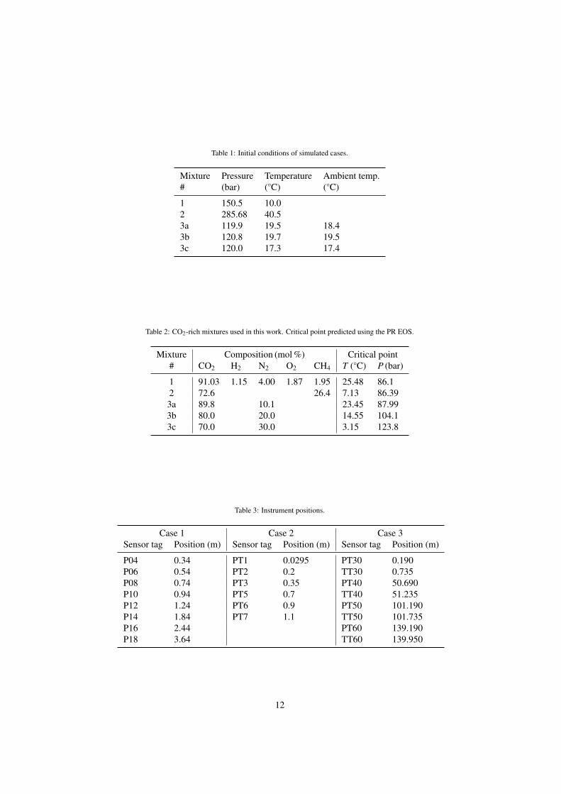
Table 1: Initial conditions of simulated cases.

Mixture Pressure Temperature Ambient temp.# (bar) (◦C) (◦C)

1 150.5 10.02 285.68 40.53a 119.9 19.5 18.43b 120.8 19.7 19.53c 120.0 17.3 17.4

Table 2: CO2-rich mixtures used in this work. Critical point predicted using the PR EOS.

Mixture Composition (mol %) Critical point# CO2 H2 N2 O2 CH4 T (◦C) P (bar)

1 91.03 1.15 4.00 1.87 1.95 25.48 86.12 72.6 26.4 7.13 86.393a 89.8 10.1 23.45 87.993b 80.0 20.0 14.55 104.13c 70.0 30.0 3.15 123.8

Table 3: Instrument positions.

Case 1 Case 2 Case 3Sensor tag Position (m) Sensor tag Position (m) Sensor tag Position (m)

P04 0.34 PT1 0.0295 PT30 0.190P06 0.54 PT2 0.2 TT30 0.735P08 0.74 PT3 0.35 PT40 50.690P10 0.94 PT5 0.7 TT40 51.235P12 1.24 PT6 0.9 PT50 101.190P14 1.84 PT7 1.1 TT50 101.735P16 2.44 PT60 139.190P18 3.64 TT60 139.950

12

t (ms)

P (

bar)

0 10 20 30 40 5020

40

60

80

100

120

140

160P04

P06

P08

P10

P12

P14

P16

P18

(a) Pressure

t (ms)

T (

°C)

0 10 20 30 40 50

­10

­5

0

5

10

15P04

P06

P08

P10

P12

P14

P16

P18

(b) Temperature

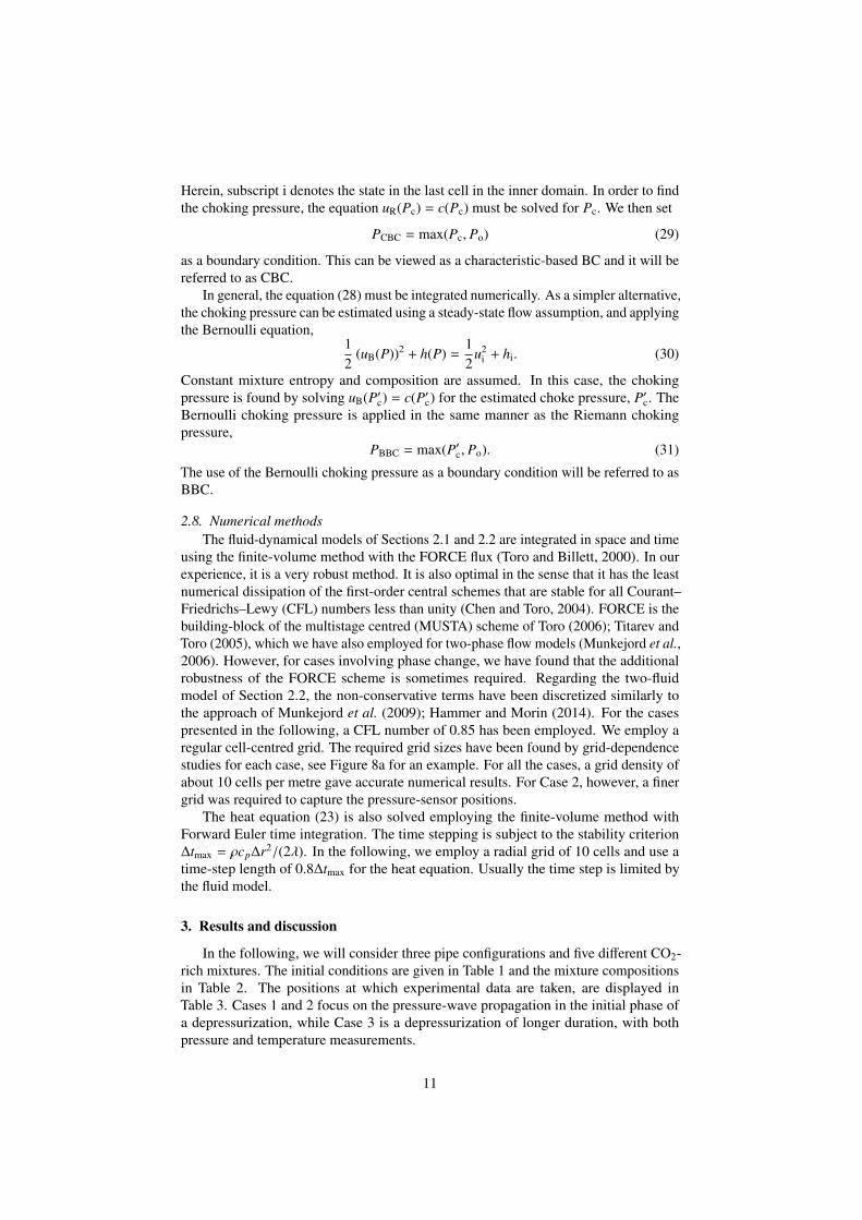
Figure 1: Case 1: Simulated quantities as a function of time at different locations. HEM.

t (ms)

P (

bar)

0 10 20 30 40 5020

40

60

80

100

120

140

160

Figure 2: Case 1: Measured pressure. After Cosham et al. (2012).

3.1. Case 1: Pressure propagation in a multi-component CO2 mixture

We will now study the propagation of pressure waves in some detail. First weconsider the case published as Test 31 by Cosham et al. (2012). A pipe of inner diameter0.146 36 m and length 144 m is filled with a mixture of 91.03 % CO2, 1.15 % H2, 4.00 %N2, 1.87 % O2 and 1.95 % CH4. The percentages are by mol. The initial pressure is149.5 barg which is about 150.51 bar and the initial temperature is 10.0 ◦C. At timet = 0, the pipe is opened to the atmosphere by the explosive cutting of a rupture disc.

The case was calculated using the HEM. Since we are only interested in the de-velopment up to time t = 50 ms, it is enough to consider the first 30 m of the pipe. Acomputational grid of 300 cells was employed. Many of the pressure sensors are closeto the open end of the pipe, where the numerical solution is sensitive to the choice ofoutlet boundary condition. Therefore, we employ the accurate BBC method, describedin Section 2.7. Since the simulated time is short, we neglect heat transfer in this case.This is also in line with the approach of Elshahomi et al. (2015). The pressure andtemperature computed at the positions given by Cosham et al. (2012), see Table 3, areplotted as a function of time in Figure 1.

The graph in Figure 1a can be compared with Figure 2, whose data we haveextracted from Figure 5 in Cosham et al. (2012). There is reasonable agreementbetween simulation and experiment, with three main points to note. First, the initial dropin pressure was faster in the simulation than in the experiment. We hypothesize that amain reason for this may be that the pipe opens instantaneously in the simulation, while

13

the opening of the bursting disc may take some time in reality. Second, the measuredpressures show plateaux which indicate phase change. These plateaux are longer inthe experiment than in the simulation. Third, the measured pressure plateaux show anincreasing trend along the pipe. There is no such trend in the simulation.

The graph in Figure 1a may also be compared with Figure 12 in Elshahomi et al.(2015). It can be seen that the results are rather similar. This is interesting to note, giventhe different numerical approaches; Elshahomi et al. (2015) employed a 2D model witha different formulation of the outlet boundary conditions, as well as a different equationof state (EOS). The most notable difference is the pressure-plateau level, which is about76 bar in the present work and about 80 bar in Elshahomi et al. (2015). This differenceis probably mainly due to the different EOS. We further observe that for this case, Jieet al. (2012) calculated a plateau pressure of about 76 bar with their model employingthe Peng–Robinson–Stryjek–Vera EOS.

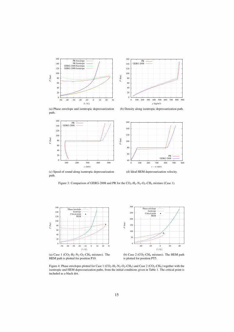
The differences between the presently employed Peng and Robinson (PR) EOS andthe GERG-2008 EOS employed by Elshahomi et al. (2015) are illustrated in Figure 3.Figure 3a shows the calculated phase envelopes and isentropic decompression pathsfor the present case. It can be observed that when using the PR EOS, the two-phasearea is encountered at a lower pressure, which is consistent with the above observations.Densities are plotted in Figure 3b. The PR EOS is seen to predict too high densitiesfor a given pressure compared to GERG-2008, especially in the upper region of thetwo-phase area. Figure 3c shows a plot of the speeds of sound. It is seen that the two-phase (mixture) speed of sound predicted by PR and GERG-2008 are not very different,but there is a substantial difference in the single-phase region. The ideal propagationvelocity of the rarefaction wave is plotted in Figure 3d. The model differences in thespeed of sound are also seen in this plot.

In Figure 4a, the isentropic and HEM depressurization paths for Case 1 are plottedtogether with the mixture phase envelope. The simulated HEM depressurization path isvery close to the ideal isentropic depressurization. This is reasonable, since there is noheat transfer in the HEM simulation, and since the effect of friction is limited.

3.2. Case 2: Pressure propagation with high initial pressure

We now consider the case and data published by Botros et al. (2013). It consists ofa tube of length 42 m and inner diameter 38.1 mm. Further details of the test facility,including sensor positions, are given in Botros (2010). The tube is filled with a mixtureconsisting of 72.6 % CO2 and 27.4 % CH4 by mol. The initial pressure is rather high, at285.68 bar, and the initial temperature is also high, at 40.5 ◦C. At the rupture of a discat the front end of the tube, a decompression wave propagates up the tube, similarly tothe preceding case.

The case has been simulated using the HEM considering the first 15 m of the tubeand employing a grid of 2400 cells. A fine grid was required to obtain a good resolutionof the sensor positions on our regular grid. The BBC boundary condition, described inSection 2.7, was employed at the outlet.

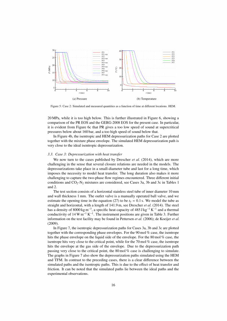
Figure 5a shows simulated and measured pressures plotted at different sensor pos-itions (see Table 3) as a function of time. The corresponding simulated temperaturescan be seen in Figure 5b. It can be observed that the simulated pressures drop fasterthan the measured ones, attaining a lower level. In view of the results of the precedingsection, and comparing with the results plotted in Figure 6 of Elshahomi et al. (2015),we hypothesize that the main reason for the discrepancy is the EOS. In particular, Fig-ure 5a indicates that the calculated decompression velocity is too low at pressures above

14

0

20

40

60

80

100

120

140

160

-50 -40 -30 -20 -10 0 10 20 30

P(b

ar)

T (°C)

PR EnvelopePR Isentrope

GERG-2008 EnvelopeGERG-2008 Isentrope

(a) Phase envelope and isentropic depressurizationpath.

0

20

40

60

80

100

120

140

160

0 100 200 300 400 500 600 700 800 900

P(b

ar)

ρ (kg/m3)

PRGERG-2008

(b) Density along isentropic depressurization path.

0

20

40

60

80

100

120

140

160

100 200 300 400 500

P(b

ar)

c (m/s)

PRGERG-2008

(c) Speed of sound along isentropic depressurizationpath.

40

60

80

100

120

140

160

0 100 200 300 400 500 600

P(b

ar)

c − u (m/s)

PRGERG-2008

(d) Ideal HEM depressurization velocity.

Figure 3: Comparison of GERG-2008 and PR for the CO2-H2-N2-O2-CH4 mixture (Case 1).

0

20

40

60

80

100

120

140

160

-50 -40 -30 -20 -10 0 10 20 30

P(b

ar)

T (°C)

Phase envelopeIsentrope

Critcal pointHEM

(a) Case 1 (CO2-H2-N2-O2-CH4 mixture). TheHEM path is plotted for position P10.

0

50

100

150

200

250

300

-40 -20 0 20 40

P(b

ar)

T (°C)

Phase envelopeIsentrope

Critcal pointHEM

(b) Case 2 (CO2-CH4 mixture). The HEM pathis plotted for position PT5.

Figure 4: Phase envelopes plotted for Case 1 (CO2-H2-N2-O2-CH4) and Case 2 (CO2-CH4) together with theisentropic and HEM depressurization paths, from the initial conditions given in Table 1. The critical point isincluded as a black dot.

15

t (ms)

P (

MP

a)

0 2 4 6 8 10

5

10

15

20

25

30PT1

PT1­exp

PT2

PT2­exp

PT3

PT3­exp

PT5

PT5­exp

PT6

PT6­exp

PT7

PT7­exp

(a) Pressure

t (ms)

T (

°C)

0 2 4 6 8 10

0

10

20

30

40PT1

PT2

PT3

PT5

PT6

PT7

(b) Temperature

Figure 5: Case 2: Simulated and measured quantities as a function of time at different locations. HEM.

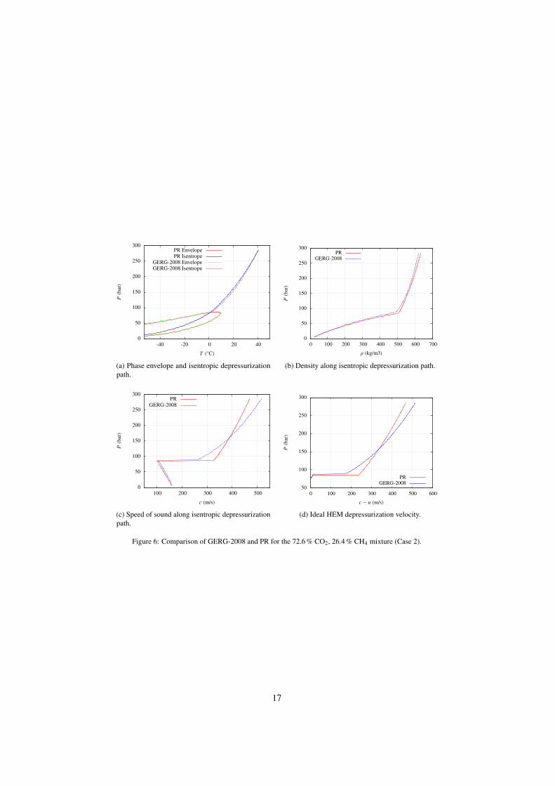
20 MPa, while it is too high below. This is further illustrated in Figure 6, showing acomparison of the PR EOS and the GERG-2008 EOS for the present case. In particular,it is evident from Figure 6c that PR gives a too low speed of sound at supercriticalpressures below about 160 bar, and a too high speed of sound below that.

In Figure 4b, the isentropic and HEM depressurization paths for Case 2 are plottedtogether with the mixture phase envelope. The simulated HEM depressurization path isvery close to the ideal isentropic depressurization.

3.3. Case 3: Depressurization with heat transferWe now turn to the cases published by Drescher et al. (2014), which are more

challenging in the sense that several closure relations are needed in the models. Thedepressurizations take place in a small-diameter tube and last for a long time, whichimposes the necessity to model heat transfer. The long duration also makes it morechallenging to capture the two-phase flow regimes encountered. Three different initialconditions and CO2-N2 mixtures are considered, see Cases 3a, 3b and 3c in Tables 1and 2.

The test section consists of a horizontal stainless steel tube of inner diameter 10 mmand wall thickness 1 mm. The outlet valve is a manually operated ball valve, and weestimate the opening time in the equation (27) to be tδ = 0.1 s. We model the tube asstraight and horizontal, with a length of 141.9 m, see Drescher et al. (2014). The steelhas a density of 8000 kg m−3, a specific heat capacity of 485 J kg−1 K−1 and a thermalconductivity of 14 W m−1 K−1. The instrument positions are given in Table 3. Furtherinformation on the test facility may be found in Pettersen et al. (2006); de Koeijer et al.(2009).

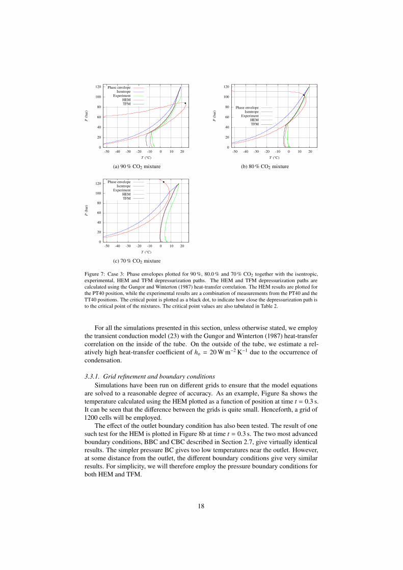
In Figure 7, the isentropic depressurization paths for Cases 3a, 3b and 3c are plottedtogether with the corresponding phase envelopes. For the 90 mol % case, the isentropehits the phase envelope on the liquid side of the envelope. For the 80 mol % case, theisentrope hits very close to the critical point, while for the 70 mol % case, the isentropehits the envelope at the gas side of the envelope. Due to the depressurization pathpassing very close to the critical point, the 80 mol % case is challenging to simulate.The graphs in Figure 7 also show the depressurization paths simulated using the HEMand TFM. In contrast to the preceding cases, there is a clear difference between thesimulated paths and the isentropic paths. This is due to the effect of heat transfer andfriction. It can be noted that the simulated paths lie between the ideal paths and theexperimental observations.

16

0

50

100

150

200

250

300

-40 -20 0 20 40

P(b

ar)

T (°C)

PR EnvelopePR Isentrope

GERG-2008 EnvelopeGERG-2008 Isentrope

(a) Phase envelope and isentropic depressurizationpath.

0

50

100

150

200

250

300

0 100 200 300 400 500 600 700

P(b

ar)

ρ (kg/m3)

PRGERG-2008

(b) Density along isentropic depressurization path.

0

50

100

150

200

250

300

100 200 300 400 500

P(b

ar)

c (m/s)

PRGERG-2008

(c) Speed of sound along isentropic depressurizationpath.

50

100

150

200

250

300

0 100 200 300 400 500 600

P(b

ar)

c − u (m/s)

PRGERG-2008

(d) Ideal HEM depressurization velocity.

Figure 6: Comparison of GERG-2008 and PR for the 72.6 % CO2, 26.4 % CH4 mixture (Case 2).

17

0

20

40

60

80

100

120

-50 -40 -30 -20 -10 0 10 20

P(b

ar)

T (°C)

Phase envelopeIsentrope

ExperimentHEMTFM

(a) 90 % CO2 mixture

0

20

40

60

80

100

120

-50 -40 -30 -20 -10 0 10 20

P(b

ar)

T (°C)

Phase envelopeIsentrope

ExperimentHEMTFM

(b) 80 % CO2 mixture

0

20

40

60

80

100

120

-50 -40 -30 -20 -10 0 10 20

P(b

ar)

T (°C)

Phase envelopeIsentrope

ExperimentHEMTFM

(c) 70 % CO2 mixture

Figure 7: Case 3: Phase envelopes plotted for 90 %, 80.0 % and 70 % CO2 together with the isentropic,experimental, HEM and TFM depressurization paths. The HEM and TFM depressurization paths arecalculated using the Gungor and Winterton (1987) heat-transfer correlation. The HEM results are plotted forthe PT40 position, while the experimental results are a combination of measurements from the PT40 and theTT40 positions. The critical point is plotted as a black dot, to indicate how close the depressurization path isto the critical point of the mixtures. The critical point values are also tabulated in Table 2.

For all the simulations presented in this section, unless otherwise stated, we employthe transient conduction model (23) with the Gungor and Winterton (1987) heat-transfercorrelation on the inside of the tube. On the outside of the tube, we estimate a rel-atively high heat-transfer coefficient of ho = 20 W m−2 K−1 due to the occurrence ofcondensation.

3.3.1. Grid refinement and boundary conditionsSimulations have been run on different grids to ensure that the model equations

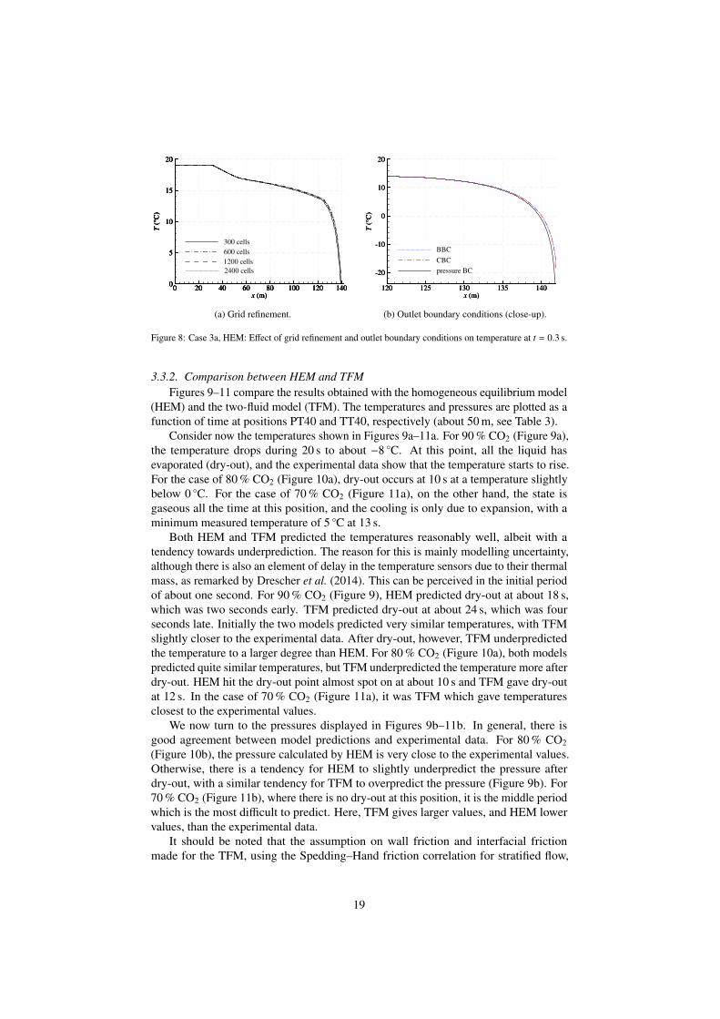
are solved to a reasonable degree of accuracy. As an example, Figure 8a shows thetemperature calculated using the HEM plotted as a function of position at time t = 0.3 s.It can be seen that the difference between the grids is quite small. Henceforth, a grid of1200 cells will be employed.

The effect of the outlet boundary condition has also been tested. The result of onesuch test for the HEM is plotted in Figure 8b at time t = 0.3 s. The two most advancedboundary conditions, BBC and CBC described in Section 2.7, give virtually identicalresults. The simpler pressure BC gives too low temperatures near the outlet. However,at some distance from the outlet, the different boundary conditions give very similarresults. For simplicity, we will therefore employ the pressure boundary conditions forboth HEM and TFM.

18

x (m)

T (

°C)

0 20 40 60 80 100 120 1400

5

10

15

20

2400 cells

x (m)

T (

°C)

0 20 40 60 80 100 120 1400

5

10

15

20

1200 cells

x (m)

T (

°C)

0 20 40 60 80 100 120 1400

5

10

15

20

600 cells

x (m)

T (

°C)

0 20 40 60 80 100 120 1400

5

10

15

20

300 cells

(a) Grid refinement.

x (m)

T (

°C)

120 125 130 135 140

­20

­10

0

10

20

pressure BC

x (m)

T (

°C)

120 125 130 135 140

­20

­10

0

10

20

CBC

x (m)

T (

°C)

120 125 130 135 140

­20

­10

0

10

20

BBC

(b) Outlet boundary conditions (close-up).

Figure 8: Case 3a, HEM: Effect of grid refinement and outlet boundary conditions on temperature at t = 0.3 s.

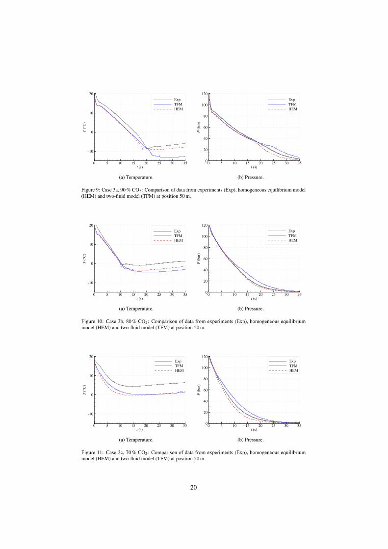
3.3.2. Comparison between HEM and TFMFigures 9–11 compare the results obtained with the homogeneous equilibrium model

(HEM) and the two-fluid model (TFM). The temperatures and pressures are plotted as afunction of time at positions PT40 and TT40, respectively (about 50 m, see Table 3).

Consider now the temperatures shown in Figures 9a–11a. For 90 % CO2 (Figure 9a),the temperature drops during 20 s to about −8 ◦C. At this point, all the liquid hasevaporated (dry-out), and the experimental data show that the temperature starts to rise.For the case of 80 % CO2 (Figure 10a), dry-out occurs at 10 s at a temperature slightlybelow 0 ◦C. For the case of 70 % CO2 (Figure 11a), on the other hand, the state isgaseous all the time at this position, and the cooling is only due to expansion, with aminimum measured temperature of 5 ◦C at 13 s.

Both HEM and TFM predicted the temperatures reasonably well, albeit with atendency towards underprediction. The reason for this is mainly modelling uncertainty,although there is also an element of delay in the temperature sensors due to their thermalmass, as remarked by Drescher et al. (2014). This can be perceived in the initial periodof about one second. For 90 % CO2 (Figure 9), HEM predicted dry-out at about 18 s,which was two seconds early. TFM predicted dry-out at about 24 s, which was fourseconds late. Initially the two models predicted very similar temperatures, with TFMslightly closer to the experimental data. After dry-out, however, TFM underpredictedthe temperature to a larger degree than HEM. For 80 % CO2 (Figure 10a), both modelspredicted quite similar temperatures, but TFM underpredicted the temperature more afterdry-out. HEM hit the dry-out point almost spot on at about 10 s and TFM gave dry-outat 12 s. In the case of 70 % CO2 (Figure 11a), it was TFM which gave temperaturesclosest to the experimental values.

We now turn to the pressures displayed in Figures 9b–11b. In general, there isgood agreement between model predictions and experimental data. For 80 % CO2(Figure 10b), the pressure calculated by HEM is very close to the experimental values.Otherwise, there is a tendency for HEM to slightly underpredict the pressure afterdry-out, with a similar tendency for TFM to overpredict the pressure (Figure 9b). For70 % CO2 (Figure 11b), where there is no dry-out at this position, it is the middle periodwhich is the most difficult to predict. Here, TFM gives larger values, and HEM lowervalues, than the experimental data.

It should be noted that the assumption on wall friction and interfacial frictionmade for the TFM, using the Spedding–Hand friction correlation for stratified flow,

19

t (s)

T (

°C)

0 5 10 15 20 25 30 35

­10

0

10

20

Exp

TFM

HEM

(a) Temperature.

t (s)

P (

bar

)

0 5 10 15 20 25 30 350

20

40

60

80

100

120

Exp

TFM

HEM

(b) Pressure.

Figure 9: Case 3a, 90 % CO2: Comparison of data from experiments (Exp), homogeneous equilibrium model(HEM) and two-fluid model (TFM) at position 50 m.

t (s)

T (

°C)

0 5 10 15 20 25 30 35

­10

0

10

20

Exp

TFM

HEM

(a) Temperature.

t (s)

P (

bar

)

0 5 10 15 20 25 30 350

20

40

60

80

100

120

Exp

TFM

HEM

(b) Pressure.

Figure 10: Case 3b, 80 % CO2: Comparison of data from experiments (Exp), homogeneous equilibriummodel (HEM) and two-fluid model (TFM) at position 50 m.

t (s)

T (

°C)

0 5 10 15 20 25 30 35

­10

0

10

20

Exp

TFM

HEM

(a) Temperature.

t (s)

P (

bar

)

0 5 10 15 20 25 30 350

20

40

60

80

100

120

Exp

TFM

HEM

(b) Pressure.

Figure 11: Case 3c, 70 % CO2: Comparison of data from experiments (Exp), homogeneous equilibriummodel (HEM) and two-fluid model (TFM) at position 50 m.

20

t (s)

T (

°C)

0 5 10 15 20 25 30 35­50

­40

­30

­20

­10

0

10

20

Exp

Transient GW

Steady GW

Transient C

(a) Temperature.

t (s)

P (

bar

)

0 5 10 15 20 25 30 350

20

40

60

80

100

120

Exp

Transient GW

Steady GW

Transient C

(b) Pressure.

Figure 12: Case 3b, 90 % CO2: Effect of heat-transfer models at position 50 m. HEM.

is somewhat coarse, although it is believed to be reasonable in a large part of thedepressurization at some distance from the outlet. Near the outlet, the gas-liquid flowwill certainly be strongly coupled, which is corroborated by the good performance ofthe HEM. In order to describe the actual flow, more comprehensive closure modelsare required. First, different flow regimes should be identified. Second, each regimeshould be modelled, accounting for friction, and momentum exchange through dropletentertainment/deposition to/from the gas phase. Development and validation of suchmodels will require detailed steady-state experimental work.

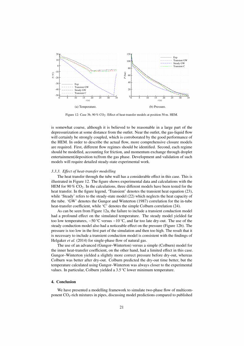
3.3.3. Effect of heat-transfer modellingThe heat transfer through the tube wall has a considerable effect in this case. This is

illustrated in Figure 12. The figure shows experimental data and calculations with theHEM for 90 % CO2. In the calculations, three different models have been tested for theheat transfer. In the figure legend, ‘Transient’ denotes the transient heat equation (23),while ‘Steady’ refers to the steady-state model (22) which neglects the heat capacity ofthe tube. ‘GW’ denotes the Gungor and Winterton (1987) correlation for the in-tubeheat-transfer coefficient, while ‘C’ denotes the simple Colburn correlation (24).

As can be seen from Figure 12a, the failure to include a transient conduction modelhad a profound effect on the simulated temperature. The steady model yielded fartoo low temperatures, −50 ◦C versus −10 ◦C, and far too late dry-out. The use of thesteady conduction model also had a noticeable effect on the pressure (Figure 12b). Thepressure is too low in the first part of the simulation and then too high. The result that itis necessary to include a transient conduction model is consistent with the findings ofHelgaker et al. (2014) for single-phase flow of natural gas.

The use of an advanced (Gungor–Winterton) versus a simple (Colburn) model forthe inner heat-transfer coefficient, on the other hand, had a limited effect in this case.Gungor–Winterton yielded a slightly more correct pressure before dry-out, whereasColburn was better after dry-out. Colburn predicted the dry-out time better, but thetemperature calculated using Gungor–Winterton was always closer to the experimentalvalues. In particular, Colburn yielded a 3.5 ◦C lower minimum temperature.

4. Conclusion

We have presented a modelling framework to simulate two-phase flow of multicom-ponent CO2-rich mixtures in pipes, discussing model predictions compared to published

21

data from depressurization experiments. In particular, two flow-model formulationshave been tested. The first is a homogeneous equilibrium model (HEM), in whichthe phases travel at the same speed. The second is a two-fluid model (TFM), wherethe difference in phasic velocities (slip) follows from friction models. This yields thepotential of including more physics. The thermodynamic properties were calculatedusing the Peng–Robinson equation of state (PR EOS).

The HEM was employed to simulate two cases where high-resolution pressure datawere available (Cases 1 and 2). Fair agreement was obtained, both with respect tothe experimental data and the 2D simulations by Elshahomi et al. (2015). The no-slipassumption in the HEM seems to be reasonable in these cases, where the two-phaseflow is presumably strongly mixed. We hypothesize that the most significant point ofimprovement for further work would be to introduce a more accurate EOS. This entailssome challenges associated to CPU time and the robust numerical solution of phaseequilibrium for multi-term EOSs. As we illustrated for Cases 1 and 2, the GERG-2008EOS gave significant differences compared to the PR EOS in key quantities, such asdensity, speed of sound and phase envelope. In the kind of computations we considerhere, such differences would affect the whole result, since all the thermodynamicquantities are coupled.

Next, depressurizations of longer duration were considered, for three different CO2-rich mixtures (Cases 3a, 3b and 3c). For cases of longer duration, the effect of heattransfer and friction becomes important. Furthermore, the cases included dry-out, whichwas captured reasonably well. For the inner heat-transfer coefficient, the simple Colburncorrelation, and the more advanced Gungor–Winterton correlation for flow boiling, weretested. Though the latter yielded somewhat better results, only moderate sensitivity forthe calculated pressure and temperature was observed. Our results clearly demonstrate,however, the necessity of considering the heat capacity of the pipe. Assuming a steady-state temperature profile in the pipe yielded far too low temperatures.

For Case 3, the HEM with the Friedel friction correlation was compared to theTFM with the Spedding–Hand friction correlation. Differences were observed in thecalculations, but based on our results, we cannot say that one gives better results thanthe other. Regarding simplicity, the HEM is preferable. We hypothesize, however,that better results could be achieved with the TFM with specially adapted models forfriction and heat transfer. The development of such models would require detailed localexperimental data.

Acknowledgements

The modelling work was performed in the CO2 Dynamics project. The authorsacknowledge the support from the Research Council of Norway (189978), GasscoAS, Statoil Petroleum AS and Vattenfall AB. The reporting was carried out in the 3DMultifluid Flow project at SINTEF Energy Research. We thank Statoil for electronicaccess to the experimental data of Drescher et al. (2014). Further, thanks are due toGelein de Koeijer and Michael Drescher of Statoil, and our colleagues Alexandre Morinand Halvor Lund, for fruitful discussions.

Kamal K. Botros of NOVA Chemicals has kindly provided the experimental data ofBotros et al. (2013) in electronic form.

22

References

Aakenes, F., Jun. 2012. Frictional pressure-drop models for steady-state and transienttwo-phase flow of carbon dioxide. Master’s thesis, Department of Energy and ProcessEngineering, Norwegian University of Science and Technology (NTNU).

Aakenes, F., Munkejord, S. T., Drescher, M., 2014. Frictional pressure drop for two-phase flow of carbon dioxide in a tube: Comparison between models and experimentaldata. Energy Procedia 51, 373–381. doi:10.1016/j.egypro.2014.07.044.

Aihara, S., Misawa, K., Jul. 2010. Numerical simulation of unstable crack propagationand arrest in CO2 pipelines. In: The First International Forum on the Transportationof CO2 by Pipeline. Clarion Technical Conferences, Gateshead, UK.

American Petroleum Institute, research project 44, 1976. Selected values of propertiesof hydrocarbons and related compounds. Thermodynamics Research Center, TexasEngineering Experiment Station, Texas A & M University, College Station, Texas,USA.

Aursand, E., Dørum, C., Hammer, M., Morin, A., Munkejord, S. T., Nordhagen, H. O.,2014. CO2 pipeline integrity: Comparison of a coupled fluid-structure model anduncoupled two-curve methods. Energy Procedia 51, 382–391. ISSN 1876-6102.doi:10.1016/j.egypro.2014.07.045.

Aursand, P., Hammer, M., Munkejord, S. T., Wilhelmsen, Ø., Jul. 2013. Pipelinetransport of CO2 mixtures: Models for transient simulation. Int. J. Greenh. Gas Con.15, 174–185. doi:10.1016/j.ijggc.2013.02.012.

Bejan, A., 1993. Heat Transfer. John Wiley & Sons, Inc., New York. ISBN 0-471-50290-1.

Bestion, D., Dec. 1990. The physical closure laws in the CATHARE code. Nucl. Eng.Design 124 (3), 229–245. doi:10.1016/0029-5493(90)90294-8.

Botros, K. K., Dec. 2010. Measurements of speed of sound in lean and rich naturalgas mixtures at pressures up to 37 MPa using a specialized rupture tube. Int. J.Thermophys. 31 (11–12), 2086–2102. doi:10.1007/s10765-010-0888-4.

Botros, K. K., Hippert, E., Jr., Craidy, P., Jun. 2013. Measuring decompression wavespeed in CO2 mixtures by a shock tube. Pipelines International 16, 22–28.

Brown, S., Martynov, S., H., M., Chen, S., Zhang, Y., 2014. Modelling the non-equilibrium two-phase flow during depressurisation of CO2 pipelines. Int. J. Greenh.Gas Con. 30, 9–18. doi:10.1016/j.ijggc.2014.08.013.

Chen, G.-Q., Toro, E. F., 2004. Centered difference schemes for non-linear hyperbolic equations. J. Hyperbolic Differ. Equ. 1 (3), 531–566.doi:10.1142/S0219891604000202.

Cosham, A., Jones, D. G., Armstrong, K., Allason, D., Barnett, J., 24–28 Sep 2012. Thedecompression behaviour of carbon dioxide in the dense phase. In: 9th InternationalPipeline Conference, IPC2012. ASME, IPTI, Calgary, Canada, vol. 3, pp. 447–464.doi:10.1115/IPC2012-90461.

23

de Koeijer, G., Borch, J. H., Jakobsen, J., Drescher, M., 2009. Experiments and modelingof two-phase transient flow during CO2 pipeline depressurization. Energy Procedia1, 1649–1656. doi:10.1016/j.egypro.2009.01.220.

Drescher, M., Varholm, K., Munkejord, S. T., Hammer, M., Held, R., de Koeijer,G., 2014. Experiments and modelling of two-phase transient flow during pipelinedepressurization of CO2 with various N2 compositions. Energy Procedia 63, 2448–2457. doi:10.1016/j.egypro.2014.11.267.

Drew, D. A., 1983. Mathematical modeling of two-phase flow. Ann. Rev. Fluid Mech.15, 261–291. doi:10.1146/annurev.fl.15.010183.001401.

Elshahomi, A., Lu, C., Michal, G., Liu, X., Godbole, A., Venton, P., 2015. Decompres-sion wave speed in CO2 mixtures: CFD modelling with the GERG-2008 equation ofstate. Appl. Energ. 140, 20–32. doi:10.1016/j.apenergy.2014.11.054.

Ely, J. F., Hanley, H. J. M., Nov. 1981. Prediction of transport properties. 1.Viscosity of fluids and mixtures. Ind. Eng. Chem. Fund. 20 (4), 323–332.doi:10.1021/i100004a004.

Ely, J. F., Hanley, H. J. M., Feb. 1983. Prediction of transport properties. 2. Thermalconductivity of pure fluids and mixtures. Ind. Eng. Chem. Fund. 22 (1), 90–97.doi:10.1021/i100009a016.

Friedel, L., Jun. 1979. Improved friction pressure drop correlations for horizontal andvertical two phase pipe flow. In: Proceedings, European Two Phase Flow GroupMeeting. Ispra, Italy. Paper E2.

Gernert, J., Span, R., 2010. EOS-CG: An accurate property model for application inCCS processes. In: Proc. Asian Thermophys. Prop. Conf. Beijing.

Giljarhus, K. E. T., Munkejord, S. T., Skaugen, G., 2012. Solution of the Span-Wagnerequation of state using a density-energy state function for fluid-dynamic simulationof carbon dioxide. Ind. Eng. Chem. Res. 51 (2), 1006–1014. doi:10.1021/ie201748a.

Gungor, K. E., Winterton, R. H. S., Mar. 1987. Simplified general correlation forsaturated flow boiling and comparisons of correlations with data. Chem. Eng. Res.Des. 65 (2), 148–156.

Hammer, M., Ervik, Å., Munkejord, S. T., 2013. Method using a density-energystate function with a reference equation of state for fluid-dynamics simulationof vapor-liquid-solid carbon dioxide. Ind. Eng. Chem. Res. 52 (29), 9965–9978.doi:10.1021/ie303516m.

Hammer, M., Morin, A., Sep. 2014. A method for simulating two-phasepipe flow with real equations of state. Comput. Fluids 100, 45–58.doi:10.1016/j.compfluid.2014.04.030.

Helgaker, J. F., Oosterkamp, A., Langelandsvik, L. I., Ytrehus, T., 2014. Validation of1D flow model for high pressure offshore natural gas pipelines. J. Nat. Gas Sci. Eng.16, 44–56. doi:10.1016/j.jngse.2013.11.001.

Hetland, J., Barnett, J., Read, A., Zapatero, J., Veltin, J., 2014. CO2 transport systemsdevelopment: Status of three large European CCS demonstration projects with EEPRfunding. Energy Procedia 63, 2458–2466. doi:10.1016/j.egypro.2014.11.268.

24

IEA, 2014. Energy Technology Perspectives. ISBN 978-92-64-20801-8.doi:10.1787/energy_tech-2014-en.

Jie, H. E., Xu, B. P., Wen, J. X., Cooper, R., Barnett, J., Sep. 2012. Predicting thedecompression characteristics of carbon dioxide using computational fluid dynamics.In: 9th International Pipeline Conference IPC2012. ASME, IPTI, Calgary, Canada,pp. 585–595. ISBN 978-0-7918-4514-1. doi:10.1115/IPC2012-90649.

Jones, D. G., Cosham, A., Armstrong, K., Barnett, J., Cooper, R., Oct. 2013. Fracture-propagation control in dense-phase CO2 pipelines. In: 6th International PipelineTechnology Conference. Lab. Soete and Tiratsoo Technical, Ostend, Belgium. Paperno. S06-02.

Klinkby, L., Nielsen, C. M., Krogh, E., Smith, I. E., Palm, B., Bernstone, C., 2011.Simulating rapidly fluctuating CO2 flow into the vedsted CO2 pipeline, injection welland reservoir. Energy Procedia 4, 4291–4298. doi:10.1016/j.egypro.2011.02.379.

Kunick, M., Kretzschmar, H.-J., Gampe, U., Sep. 2008. Fast calculation of thermody-namic properties of water and steam in process modelling using spline interpolation.In: Proceedings 15th International Conference on the Properties of Water and Steam,ICPWS XV. Berlin, Germany.

Kunz, O., Wagner, W., October 2012. The GERG-2008 wide-range equation of state fornatural gases and other mixtures: An expansion of GERG-2004. J. Chem. Eng. Data57 (11), 3032–3091. doi:10.1021/je300655b.

Li, H., Jakobsen, J. P., Wilhelmsen, Ø., Yan, J., Nov. 2011a. PVTxy properties ofCO2 mixtures relevant for CO2 capture, transport and storage: Review of avail-able experimental data and theoretical models. Appl. Energ. 88 (11), 3567–3579.doi:10.1016/j.apenergy.2011.03.052.

Li, H., Wilhelmsen, Ø., Lv, Y., Wang, W., Yan, J., Sep. 2011b. Viscosity,thermal conductivity and diffusion coefficients of CO2 mixtures: Review of ex-perimental data and theoretical models. Int. J. Greenh. Gas Con. 5 (5), 1119–1139.doi:10.1016/j.ijggc.2011.07.009.

Liou, M.-S., Steffen, C. J., Jr., 1993. A new flux splitting scheme. J. Comput. Phys.107 (1), 23–39. doi:10.1006/jcph.1993.1122.

Mahgerefteh, H., Brown, S., Denton, G., May 2012. Modelling the impact of streamimpurities on ductile fractures in CO2 pipelines. Chem. Eng. Sci. 74, 200–210.doi:10.1016/j.ces.2012.02.037.

Michelsen, M. L., 1999. State function based flash specifications. Fluid Phase Equilib.158-160, 617–626. doi:10.1016/S0378-3812(99)00092-8.

Michelsen, M. L., Mollerup, J. M., 2007. Thermodynamic models: Fundamentals &

computational aspects. Tie-Line Publications, Holte, Denmark, second ed. ISBN87-989961-3-4.

Morin, A., Flåtten, T., 2012. A two-fluid four-equation model with instantan-eous thermodynamical equilibrium. Submitted URL http://www.stat.ntnu.no/conservation/2013/002.pdf.

25

Munkejord, S. T., Jul. 2006. Partially-reflecting boundary conditions for transienttwo-phase flow. Commun. Numer. Meth. En. 22 (7), 781–795. doi:10.1002/cnm.849.

Munkejord, S. T., Bernstone, C., Clausen, S., de Koeijer, G., Mølnvik, M. J., 2013.Combining thermodynamic and fluid flow modelling for CO2 flow assurance. EnergyProcedia 63, 2904–2913. doi:10.1016/j.egypro.2013.06.176.

Munkejord, S. T., Evje, S., Flåtten, T., Oct. 2006. The multi-stage centred-schemeapproach applied to a drift-flux two-phase flow model. Int. J. Numer. Meth. Fl. 52 (6),679–705. doi:10.1002/fld.1200.

Munkejord, S. T., Evje, S., Flåtten, T., Jun. 2009. A MUSTA scheme for anonconservative two-fluid model. SIAM J. Sci. Comput. 31 (4), 2587–2622.doi:10.1137/080719273.

Munkejord, S. T., Jakobsen, J. P., Austegard, A., Mølnvik, M. J., Jul. 2010. Thermo- andfluid-dynamical modelling of two-phase multi-component carbon dioxide mixtures.Int. J. Greenh. Gas Con. 4 (4), 589–596. doi:10.1016/j.ijggc.2010.02.003.

NETL, Aug. 2013. CO2 impurity design parameters. Tech. Rep. DOE/NETL-341-011212, National Energy Technology Laboratory, USA.

Nordhagen, H. O., Kragset, S., Berstad, T., Morin, A., Dørum, C., Munkejord, S. T.,Mar. 2012. A new coupled fluid-structure modelling methodology for running ductilefracture. Comput. Struct. 94–95, 13–21. doi:10.1016/j.compstruc.2012.01.004.

Paillère, H., Corre, C., García Cascales, J. R., Jul. 2003. On the extension of theAUSM+ scheme to compressible two-fluid models. Comput. Fluids 32 (6), 891–916.doi:10.1016/S0045-7930(02)00021-X.

Peng, D. Y., Robinson, D. B., Feb. 1976. A new two-constant equation of state. Ind.Eng. Chem. Fund. 15 (1), 59–64. doi:10.1021/i160057a011.

Pettersen, J., de Koeijer, G., Hafner, A., Jun. 2006. Construction of a CO2 pipeline testrig for R&D and operator training. In: GHGT-8 – 8th International Conference onGreenhouse Gas Control Technologies. Trondheim, Norway.

Pini, M., Spinelli, A., Persico, G., Rebay, S., 2015. Consistent look-up table in-terpolation method for real-gas flow simulations. Comput. Fluids 107, 178–188.doi:10.1016/j.compfluid.2014.11.001.

Spedding, P. L., Hand, N. P., 1997. Prediction in stratified gas-liquid co-current flow inhorizontal pipelines. Int. J. Heat Mass Tran. 40 (8), 1923–1935. doi:10.1016/S0017-9310(96)00252-9.

Stryjek, R., Vera, J. H., 1986. PRSV: An improved Peng–Robinson equation ofstate for pure compounds and mixtures. Can. J. Chem. Eng. 64 (2), 323–333.doi:10.1002/cjce.5450640224.

Stuhmiller, J. H., Dec. 1977. The influence of interfacial pressure forces on the char-acter of two-phase flow model equations. Int. J. Multiphase Flow 3 (6), 551–560.doi:10.1016/0301-9322(77)90029-5.

Swesty, F., 1996. Thermodynamically consistent interpolation for equation of statetables. J. Comput. Phys. 127 (1), 118–127. doi:10.1006/jcph.1996.0162.

26

Timmes, F. X., Swesty, F. D., 2000. The accuracy, consistency, and speed of an electron-positron equation of state based on table interpolation of the Helmholtz free energy.Astrophys. J. Suppl. S. 126 (2), 501–516. doi:10.1086/313304.

Titarev, V. A., Toro, E. F., Sep. 2005. MUSTA schemes for multi-dimensional hyperbolicsystems: analysis and improvements. Int. J. Numer. Meth. Fl. 49 (2), 117–147.doi:10.1002/fld.980.

Toro, E. F., Oct.–Nov. 2006. MUSTA: A multi-stage numerical flux. Appl. Numer. Math.56 (10–11), 1464–1479. doi:10.1016/j.apnum.2006.03.022.

Toro, E. F., Billett, S. J., Nov. 2000. Centred TVD schemes for hyperbolic conservationlaws. IMA J. Numer. Anal. 20 (1), 47–79. doi:10.1093/imanum/20.1.47.

US DOE, 2010. Interagency Task Force on Carbon Capture and Storage. Washington,DC, USA.

Wareing, C. J., Fairweather, M., Falle, S. A. E. G., Woolley, R. M., 2014. Validationof a model of gas and dense phase CO2 jet releases for carbon capture and storageapplication. Int. J. Greenh. Gas Con. 20, 254–271. doi:10.1016/j.ijggc.2013.11.012.

Xia, G., Li, D., Merkle, C. L., 2007. Consistent properties reconstruction on adaptivecartesian meshes for complex fluids computations. J. Comput. Phys. 225 (1), 1175–1197. doi:10.1016/j.jcp.2007.01.034.

Xu, B. P., Jie, H. E., Wen, J. X., 2014. A pipeline depressurization model forfast decompression and slow blowdown. Int. J. Pres. Ves. Pip. 123–124, 60–69.doi:10.1016/j.ijpvp.2014.07.003.

27