Deploying Multiple Interconnected Gateways in

Heterogeneous Wireless Sensor Networks: an

Optimization Approach

Antonio Capone∗ , Matteo Cesana, Danilo De Donno, Ilario Filippini

Politecnico di MilanoDipartimento di Elettronica ed InformazionePiazza L. da Vinci 32, 20133 Milan, Italy

Abstract

Data collected by sensors often have to be remotely delivered through multi-hop wireless paths to data sinks connected to application servers for infor-mation processing. The position of these sinks has a huge impact on thequality of the specific Wireless Sensor Network (WSN). Indeed, it may cre-ate artificial traffic bottlenecks which affect the energy efficiency and theWSN lifetime. This paper considers a heterogeneous network scenario wherewireless sensors deliver data to intermediate gateways geared with a diversewireless technology and interconnected together and to the sink. An opti-mization framework based on Integer Linear Programming (ILP) is developedto locate wireless gateways minimizing the overall installation cost and theenergy consumption in the WSN, while accounting for multi-hop coveragebetween sensors and gateways, and connectivity among wireless gateways. Atraffic-variable scenario is also considered, where the network can go throughhigh and low traffic operation points, and the topology is optimized accord-ingly. The proposed ILP formulations are solved to optimality for medium-size instances to analyze the quality of the designed networks, and heuristicalgorithms are also proposed to tackle large-scale heterogeneous scenarios.

Key words: Wireless Sensor Networks, Gateway Placement, Optimization

Email address: <surname>@elet.polimi.it (Antonio Capone∗ , Matteo Cesana,Danilo De Donno, Ilario Filippini)

∗Corresponding author.

Preprint submitted to Computer Communications October 28, 2013

1. Introduction

Wireless Sensor Networks (WSN) have recently emerged as an ideal so-lution to a large number of applications where the goal is collecting mea-surements of a physical parameters (temperature, humidity, light intensity,etc.) or detecting events in the covered area (intrusion, wild fire, etc.) [3].Sensors are usually low-cost battery-operated devices geared with sensing,processing and communication functionalities. Obviously, the limited energyavailability deeply impacts on the design of WSN and in particular on com-munication protocols running at different levels [4, 5, 6] as well as on networkdeployment [7, 8] and topology.

In many scenarios, data collected by sensors must be delivered to appli-cation servers for processing. These servers can be reached via a sink nodethat is connected to a local or geographical network through a communica-tion interface with a different technology with respect to the WSN. Sincethe transmission range of sensor nodes is often much smaller than the areacovered by the WSN, sensors cooperate to deliver information to the sinknode through multi-hop paths.

Multi-hop information delivery to sink nodes requires multiple transmis-sions that consume energy in intermediate nodes and heavily limit lifetime ofthose nodes that are used more frequently. Even if many routing approacheshave been proposed to balance the load among nodes and prolong the overallnetwork lifetime, it is quite evident that nodes closer to the sink are anywaythe most critical ones since they are required to relay all traffic generated bythe other nodes and headed to the sink. For this reason, several methodshave been proposed for optimizing the sink position in WSN design [15, 17].

However, a single sink node collecting all data from the network is not anefficient solution when dealing with large size WSNs, like e.g. in applicationsfor monitoring natural areas. Indeed, as the network grows, the amount ofinformation that must be delivered to the sink by surrounding nodes increasescreating traffic and energy consumption bottlenecks. A promising alternativeapproach is based on the use of additional concentration nodes, gateways,that allow to spread the load and also to keep multi-hop paths within areasonable length [10, 11, 12]. Also in this case gateway positioning is a keyelement for designing efficient networks. The entire set of sensor nodes needto be divided into independent subsets that send their traffic to a gateway,giving rise to a clustering problem.

Generally speaking, gateways are more powerful and expensive devices

2

with respect to sensors and a reasonable objective is minimizing their numberwhile matching constraints on energy efficiency and network quality [10, 12,14]. However, this approach focuses on the WSN only neglecting the problemof interconnecting the gateways to the sink or more in general to the networkwhere application servers are located. According to the specific applicationscenario, several solutions can be adopted for this problem, including the useof direct geographical links among the gateways (wired links, satellite links,etc.). However, this may be quite expensive and inefficient, since the trafficcollected at each gateway is usually much smaller than the link capacity whileits cost (interface, installation, and operation) often high.

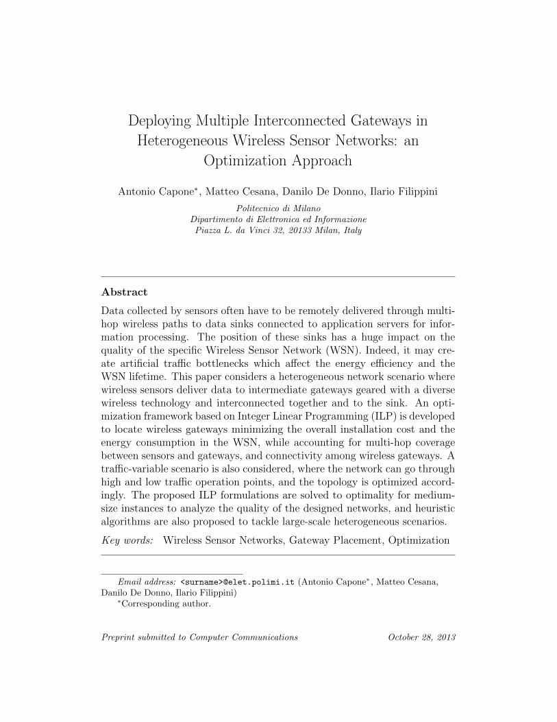
For this reason, we consider an alternative network scenario where gate-ways are inter-connected through a Wireless Mesh Network (WMN) and actas Wireless Routers (WRs) forwarding traffic along multi-hop paths toward asink node that is the only one equipped with a geographical link (see Figure1). The resulting architecture is an heterogenous multi-hop network with dif-ferent devices (sensors, WRs, and sink points) and wireless links (low-powerlow-rate links for sensors, and high rate links for mesh routers) that can beadapted to the specific application scenario using available technologies (likee.g. ZigBee, WiFi, WiMax, etc.)

In the aforementioned scenario, we investigate the joint problem of se-lecting/positioning the gateways (WRs) and designing the WMN that inter-connects them. We provide an optimization framework that minimizes in-stallation costs and maximizes the energy efficiency, while considering bothmulti-hop coverage and connectivity constraints. Coverage considers theavailability of a multi-hop path between each sensor node and at least agateway, while connectivity among gateways must be ensured by properlydesigning the WMN. The proposed optimization framework is independenton the specific routing strategy in the WSN; indeed, routes in the WSN (fromsensors to gateways) are assumed to be given. This allows to use any of therouting mechanisms that have been proposed for WSNs [5] and to plug itinto our optimization framework just modifying a separate software modulethat computes traffic loads in the WSN. We note here that routing could beeasily optimized together with gateway positions by including further degreesof freedom (variables) in the optimization framework [10, 14, 26]. However,we believe that our approach is more practical since in real-life wireless sen-sor networks the network installer can hardly modify/optimize the routingschemes running in the specific WSNs technology.

We propose an Integer Linear Programming (ILP) framework that allows

3

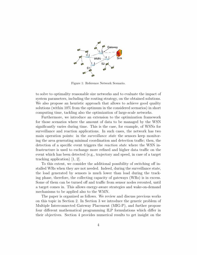
Figure 1: Reference Network Scenario.

to solve to optimality reasonable size networks and to evaluate the impact ofsystem parameters, including the routing strategy, on the obtained solutions.We also propose an heuristic approach that allows to achieve good qualitysolutions (within 10% from the optimum in the considered scenarios) in shortcomputing time, tackling also the optimization of large-scale networks.

Furthermore, we introduce an extension to the optimization frameworkfor those scenarios where the amount of data to be managed by the WSNsignificantly varies during time. This is the case, for example, of WSNs forsurveillance and reaction applications. In such cases, the network has twomain operation points: in the surveillance state the sensors keep monitor-ing the area generating minimal coordination and detection traffic; then, thedetection of a specific event triggers the reaction state where the WSN in-frastructure is used to exchange more refined and higher data traffic on theevent which has been detected (e.g., trajectory and speed, in case of a targettracking application) [1, 2].

To this extent, we consider the additional possibility of switching off in-stalled WRs when they are not needed. Indeed, during the surveillance state,the load generated by sensors is much lower than load during the track-ing phase, therefore, the collecting capacity of gateways (WRs) is in excess.Some of them can be turned off and traffic from sensor nodes rerouted, untila target comes in. This allows energy-aware strategies and wake-on-demandmechanisms to be applied also to the WMN.

The paper is organized as follows. We review and discuss previous workson this topic in Section 2. In Section 3 we introduce the generic problem ofMultiple Interconnected Gateway Placement (MIG-P), and further proposefour different mathematical programming ILP formulations which differ intheir objectives. Section 4 provides numerical results to get insight on the

4

characteristics of the optimal solutions obtained through the ILP framework.The heuristic algorithms proposed for tackling large size instances and resultsto assess their performance are presented in Section 5. We conclude the paperin Section 6.

2. Related work

The Gateway Placement problem has been extensively studied in liter-ature [25]. The whole set of works can be divided into two classes. Oneis the class of Static Base Station Positioning problems where the WSN isdeployed, gateways are installed and their positions never change for the en-tire network lifetime. The other class, the class of Dynamic Base StationPositioning problems is characterized by the gateway re-positioning duringthe network operation. The latter type of problems investigate the way ofmoving gateways to react in front of topology changes, failures, new QoS pa-rameters or simply to balance the energy consumption among sensor nodes.Even though many works of this class exist [13, 20, 22], this type of problemsis out of the scope of our work.

We focus on the class of Static Base Station Positioning problems. Someapproaches consider the best placement of a single sink node. In [15] authorspropose an iterative repositioning geometric algorithm to find the best sinklocation in terms of minimum overall transmission energy. However, theyassume the gateway is always reachable within a single hop. General sensor-sink paths are considered in [17] where an approximated algorithm aims tomaximize the lifetime of a single-sink WSN.

When more gateways are available the problem gets harder because bothpositions and number of installed gateways must be chosen. The installationof multiple gateways induces the partition of the WSN into clusters, each oneassigned to a gateway. Authors in [18] study the problem of positioning thesmallest number of gateways in such a way sensors are covered in a singlehop by gateway and the set of gateways forms a connected network. Theypropose a solution approach that divides the deployment area in square cells,finds the best single gateway placement for each cell, and then connects cellsinstalling, if required, new gateways. It does not include any energy issueand lack in multi-hop paths between sensors and gateways.

In [12] heuristic algorithms based on local search and greedy techniquesare proposed. Their objective is finding the best sensor nodes to be selectedas gateways. The selection of the fixed number of gateways aims to minimize

5

the overall energy consumption. Authors in [11] propose ILP models. Theydefine several versions of the Gateway Placement problem that minimize thenumber of gateways with a coverage requirement or minimize path lengthsfrom nodes to gateways with an installation budget and coverage constraints.However, these approaches do not guarantee connectivity among gatewaysand/or pay not attention to the load of critical nodes.

The work in [19] present ILP models where energy issues are expressedas limits on the cluster size and the number of hops between a node and agateway. Authors in [10] propose an ILP model. The objective is minimizingthe maximum number of transmitted/received packets at each sensor node.Given a fixed number of gateways, the solution provides optimum gatewayplacement and flows along links. The work in [14] presents Linear Program-ming (LP) models that maximize the total throughput during the networklifetime with fairness guarantees. Solutions provide gateway positions anddata rate values. The last three modeling aproaches, besides not addressgateway connectivity, force the selection of optimized routing paths.

Some further works start from a planned network and try to improvethe topology according to some energy-aware principles. Although they donot consider an actual placement problem, they are interesting because oftheir approaches to energy-aware sensor clustering. Authors in [16] considerthe problem of adding a given amount of energy to the WSN, expressed asgateways to be properly located in the area, in order to extend the networklifetime. In [9] a node-gateway assignment algorithm is proposed. It aims atdistributing evenly the number of nodes among gateways. In [21], instead,the assignment algorithm is a genetic algorithm aiming at minimizing thetotal number of hops within the network.

3. The Multiple Interconnected Gateway Placement Problem

We consider a heterogeneous network scenario where clouds of WirelessSensor Networks (WSNs) for data collection are connected to a sink nodethrough a wireless mesh backbone of gateway devices. We will use gatewaysand WRs as synonyms throughout the paper. Each WR acts as a trafficconcentration point for all the sensor nodes belonging to the correspondingWSN. In such network scenario, the number and the positions of the WRsobviously impact on the wireless sensor network lifetime. In fact, roughlyspeaking, placing a WR in a given position increases the load of all the sensorsin the one-hop neighborhood, which are forced to relay to the gateway also

6

the traffic coming from the leaves sensors. We will call these sensor nodescritical nodes with respect to a given WR (e.g., nodes S1 and S2 in Fig. 1are critical nodes).

In this work, we aim at optimizing the overall network topology by prop-erly selecting number and locations of WRs in such a way that installationcosts are minimized and energy efficiency maximized, under the constraintsthat each sensor must be connected through a multi-hop path to the clos-est WR (to limit energy consumption due to packet forwarding), and that amulti-hop path does exist also between each WR and the traffic sink. There-fore, the optimization framework jointly considers the selection/positioningof WRs, as well as the design of the WMN among WRs.

We take a constructive approach in presenting the mathematical pro-gramming framework. Indeed, we introduce first a basic formulation of theMIG-P problem which considers only installation cost minimization whileensuring coverage within a maximum number of hops of all the sensors andconnectivity between gateways and sink node (Sec. 3.1); then, we extend thebasic formulation to an energy-aware formulation which also minimizes theload of critical nodes (Sec. 3.2). Then, a budget formulation which considersa budget constraint on the number of installed WRs is presented. The goal ismaximizing the network lifetime selecting the best locations where availableWRs must be installed (Sec. 3.3). Finally, the forth version of the prob-lem faces a bi-state scenario. In this case the formulation jointly determinesthe number and positions of WRs to be installed during the high-load stateand which of them to be switched off during the low-load state in order tominimize total costs (Sec. 3.4).

3.1. Basic Formulation

The WSN can be represented as a set of test points S = {1..NS} in thenetwork, whereas a set of candidate sites, denoted by W = {1..NW}, definesthe potential positions where WRs can be installed. Each WR can establish awireless link with any other WR at a distance smaller than its communicationrange RW on the backbone, as well as with any sensor at distance lower thanRC in the WSN3. According to that, we define an adjacency matrix that

3The link definition on the basis of a communication range is only for the sake ofpresentation. We note here that the proposed framework holds for any type of connectivitymatrix.

7

summarizes connectivity among candidate sites:

Iij =

{1 if i ∈ W , j ∈ W , dist(i, j) ≤ RW

0 otherwise

where dist(·) is the Euclidean distance between the positions of the twoinvolved devices.

The routing pattern is an input parameter of the optimization problem.Given a candidate site, the specific routing strategy adopted in the WSNdetermines the assignment of sensor nodes to gateways, as well as the set ofmulti-hop paths used for collecting data. To represent the concept of multi-hop coverage, we introduce the following binary matrix C, which indicateswhether each sensor is connected through a multi-hop path to a given WR:

Cij =

1 if there exists a route from sensor node i and WR j

with no more than MAXHOPS hops0 otherwise

being MAXHOPS is the maximum allowed number of hops of a route.In addition, for each sensor node i we define the ordered vector Oi of

the reachable WRs. The ordering relation is such that given two WRs,one at the j-th place, Oi(j), and one at the k-th, Oi(k), if j < k thendist(i, j) ≤ dist(i, k). Sets Ji are index sets of vectors Oi.

We introduce the following sets of decision variables defining WR instal-lation, node-gateway assignment and routing in the WMN. In detail:

yi =

{1 if a WR is installed in candidate site i0 otherwise

xij =

1 if sensor node i is assigned to WR j,

that is, node i routes its traffic toward WR j0 otherwise

fij are integer flow variables for links (i, j), i, j ∈ S in the WMN formed byinstalled WRs, while the fw represents the overall traffic entering the sinknode.

The proposed ILP model for the basic formulation of the MIG-P problem

8

is:

min∑i∈W

yi (1)

s.t.∑j∈W

xij = 1 ∀ i ∈ S (2)

xij ≤ Cijyj ∀ i ∈ S, j ∈ W (3)∑i∈S

xij +∑l∈W

(flj − fjl) =

{fw, if j = SINK0, otherwise

∀ j ∈ W (4)

fij ≤ NSIijyi, fij ≤ NSIijyj ∀ i, j ∈ W (5)

yOi(k) +∑

h∈Ji,h>k

xiOi(h) ≤ 1 ∀ i ∈ S, k ∈ Ji (6)

yi ∈ {0, 1} , xhj ∈ {0, 1} , fij ∈ Z+, fw ∈ Z+ ∀i, j ∈ W , ∀h ∈ S(7)

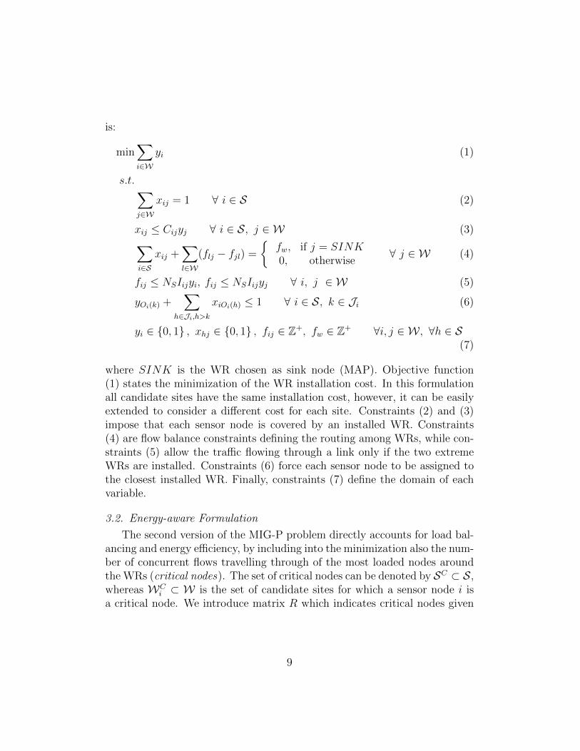
where SINK is the WR chosen as sink node (MAP). Objective function(1) states the minimization of the WR installation cost. In this formulationall candidate sites have the same installation cost, however, it can be easilyextended to consider a different cost for each site. Constraints (2) and (3)impose that each sensor node is covered by an installed WR. Constraints(4) are flow balance constraints defining the routing among WRs, while con-straints (5) allow the traffic flowing through a link only if the two extremeWRs are installed. Constraints (6) force each sensor node to be assigned tothe closest installed WR. Finally, constraints (7) define the domain of eachvariable.

3.2. Energy-aware Formulation

The second version of the MIG-P problem directly accounts for load bal-ancing and energy efficiency, by including into the minimization also the num-ber of concurrent flows travelling through of the most loaded nodes aroundthe WRs (critical nodes). The set of critical nodes can be denoted by SC ⊂ S,whereas WC

i ⊂ W is the set of candidate sites for which a sensor node i isa critical node. We introduce matrix R which indicates critical nodes given

9

the specific routing algorithm:

Ri,gc =

1 if route from node i to WR g goes through node c

(node c is a critical node for the path from node i to WR g)0 otherwise

The number of paths through a critical node i is given by the additionalvariable pi,∀i ∈ SC .

The new ILP model consists in replacing objective function (1) with thefollowing:

min∑i∈W

yi + α∑j∈SC

pj (8)

and including the additional constraints:∑j∈S:j 6=i

Rj,ci xjc ≤MPxic + pi ∀i ∈ SC , c ∈ WC

i (9)

pi ∈ Z+ ∀i ∈ SC (10)

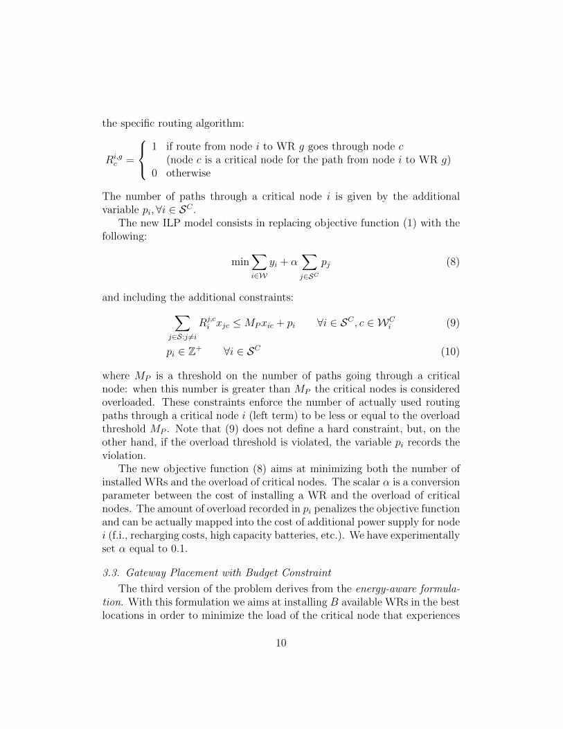
where MP is a threshold on the number of paths going through a criticalnode: when this number is greater than MP the critical nodes is consideredoverloaded. These constraints enforce the number of actually used routingpaths through a critical node i (left term) to be less or equal to the overloadthreshold MP . Note that (9) does not define a hard constraint, but, on theother hand, if the overload threshold is violated, the variable pi records theviolation.

The new objective function (8) aims at minimizing both the number ofinstalled WRs and the overload of critical nodes. The scalar α is a conversionparameter between the cost of installing a WR and the overload of criticalnodes. The amount of overload recorded in pi penalizes the objective functionand can be actually mapped into the cost of additional power supply for nodei (f.i., recharging costs, high capacity batteries, etc.). We have experimentallyset α equal to 0.1.

3.3. Gateway Placement with Budget Constraint

The third version of the problem derives from the energy-aware formula-tion. With this formulation we aims at installing B available WRs in the bestlocations in order to minimize the load of the critical node that experiences

10

the highest load, so as to maximize the network lifetime. A new variable mis introduced to store the maximum number of paths going trough a criticalnode (the maximum value of variables pi in the network: ∀i ∈ SC). We re-port below the complete formulation for the gateway placement with budgetconstraint.

min m (11)

s.t.∑j∈W

xij = 1 ∀ i ∈ S (12)

xij ≤ Cijyj ∀ i ∈ S, j ∈ W (13)∑i∈S

xij +∑l∈W

(flj − fjl) =

{fw, if j = SINK0, otherwise

∀ j ∈ W (14)

fij ≤ NSIijyi, fij ≤ NSIijyj ∀ i, j ∈ W (15)

yOi(k) +∑

h∈Ji,h>k

xiOi(h) ≤ 1 ∀ i ∈ S, k ∈ Ji (16)∑j∈S:j 6=i

Rj,ci xjc ≤MPxic + pi ∀i ∈ SC , c ∈ WC

i (17)∑j∈CS

yi ≤ B (18)

m ≥ pi ∀i ∈ SC (19)

yi ∈ {0, 1} , xhj ∈ {0, 1} , fij ∈ Z+, fw ∈ Z+, pk ∈ Z+,m ∈ Z+

∀i, j ∈ W , ∀h ∈ S, ∀k ∈ SC (20)

The objective function (11) aims at minimizing the maximum number ofpaths going through a critical node. Constraints (12)-(17) and (20) have thesame meaning as in the previous formulations, while new constraints (18)and (19), respectively, state the maximum number of deployable WRs (abudget of B devices) and define the correct value of variable m.

3.4. Bi-state scenario

In this version of the problem the network scenario consists of two states.A low state where the amount of data generated by sensor nodes is small (e.g.,WSN during surveillance phase) and a high state where sensor nodes injecta high level of traffic into the network (e.g., WSN during tracking phase). In

11

such a scenario, capacity issues, which usually are not of high importance inWSNs, become crucial due to high loads network must sustain.

The objective of the proposed formulation is to design a WMN placingWRs in order to collect the total traffic generated during the high stateand select which of the installed WRs can be switched off during the lowstate, provided that connectivity and capacity constraints are satisfied in bothphases. The aim is minimizing total costs that include both WR installationand WR operation costs. Installation costs are related to the placement of aWR in a given site, while operation costs refer to costs needed to keep WRsoperative (f.i, power supply cost). Given two variable sets yj, j ∈ W andsj, j ∈ W defined as

yi =

{1 if a WR is installed in candidate site i0 otherwise

and

zi =

{1 if WR in candidate site i is switched off during the low state0 otherwise,

the objective function of the bi-state formulation is

min∑j∈W

CINSTj yj +

∑j∈W

CONTNET

(yj − SOFF zj

)(21)

where CINSTj is the cost of installing a WR in candidate site j, CON is the

operation cost per time unit of a WR during the high state, TNET is the timethe network is expected to be operative, and SOFF is the cost saving whena WR is turned off during low state, expressed as a fraction of the operationcost CON . In first approximation, we can write SOFF as a function of thedurations of each phase and operation costs. We can write

SOFF =CON − COFF

CON

TLTH + TL

where CON and COFF are the operation costs per time unit when a WRis active and inactive, respectively, while TH and TL are the expected totalduration of high state and low state, TH + TL = TNET .

In order to define the set of constraints a solution must be subject to, weintroduce two further groups of variables, one for each state. The first group

12

consists of variables that describe the network during the high state.

xHij =

1 if sensor node i is assigned to WR j during high state,

that is, node i routes its traffic toward WR j0 otherwise

fHij are rationale flow variables for links (i, j), i, j ∈ S in the WMN formed

by installed WRs, while the fHw represents the overall traffic entering the sink

node. The second group contains the same sets of variables, but referringto the low state: xLij, fLij, and fL

w . Beside variables, some parametersdescribe traffic and capacity values. DL

i and DHi express the amount of

traffic generated by sensor node i during, respectively, low state and highstate, while NCAP states node capacity in terms of incident traffic load. Nowwe can write the whole formulation:

min∑j∈W

CINSTj yj +

∑j∈W

CONTNET

(yj − SOFF zj

)(22)

s.t.

yj ≥ zj ∀j ∈ W (23)∑j∈W

xHij = 1 ∀ i ∈ S (24)

xHij ≤ Cijyj ∀ i ∈ S, j ∈ W (25)∑i∈S

DHi x

Hij +

∑l∈W

(fHlj − fH

jl ) =

{fHw , if j = SINK0, otherwise

∀ j ∈ W

(26)

fHij ≤

(∑h∈S

DHh

)Iijyi, f

Hij ≤

(∑h∈S

DHh

)Iijyj ∀ i, j ∈ W (27)

13

yOi(k) +∑

h∈Ji,h>k

xHiOi(h)≤ 1 ∀ i ∈ S, k ∈ Ji (28)∑

j∈S:j 6=i

Rj,ci D

Hj x

Hjc ≤ NCAPx

Hic ∀i ∈ SC , c ∈ WC

i (29)∑j∈W

xLij = 1 ∀ i ∈ S (30)

xLij ≤ Cij (yj − zj) ∀ i ∈ S, j ∈ W (31)∑i∈S

DLi x

Lij +

∑l∈W

(fLlj − fL

jl) =

{fLw , if j = SINK0, otherwise

∀ j ∈ W (32)

fLij ≤

(∑h∈S

DLh

)Iij (yi − zi) , fL

ij ≤

(∑h∈S

DLh

)Iij (yj − zj)

∀ i, j ∈ W (33)

yOi(k) +∑

h∈Ji,h>k

xLiOi(h)≤ 1 ∀ i ∈ S, k ∈ Ji (34)∑

j∈S:j 6=i

Rj,ci D

Lhx

Ljc ≤ NCAPx

Lic ∀i ∈ SC , c ∈ WC

i (35)

yi ∈ {0, 1} , zi ∈ {0, 1} , xHhi ∈ {0, 1} , xLhi ∈ {0, 1} , ∀i ∈ W , ∀h ∈ S(36)

fHij ∈ Z+, fH

w ∈ Z+, fLij ∈ Z+, fL

w ∈ Z+ ∀i, j ∈ W (37)

Constraints (23) force a WR to be already installed before being switchedoff during the low state. Constraints (24)-(28) correspond to constraints (2)-(6) of the basic formulation, while constraints (29) force the total amount oftraffic going through a node to be below its capacity. Constraints (24)-(29)include variables related to high state, similarly, constraints (30)-(35) havethe same meaning but refer to low state variables. Note that quantity yi− ziis not zero only if the WR at site i is installed and not turned off during thelow state.

Finally, note that we can model the complete shutdown of a sensor noden̂ during low state by setting DL

n̂ of such nodes equal to 0 and modifyingrelated constraint (30) in

∑j∈W x

Ln̂j = 0.

14

4. Optimal Gateway Placement

We have tested the quality of the planned heterogeneous WSNs under twodifferent routing algorithms: a classical min-hop shortest path, and an idealenergy-aware routing. In the latter case, routing paths are obtained solvinga Minimum Cost Flow problem towards each candidate site, where the bestrouting paths from every sensor to a given candidate site are determined ac-cording to the following objective function: min

∑(i,j)∈L dist(i, j)flowij + βmC ,

where L is the set of wireless links among sensor nodes and the gatewaylocated at the site, flowij are variables defining the number of node-gatewaypaths through link (i, j) and mC expresses the number of routing paths goingthrough the most loaded critical node. Note that the obtained routes pre-serve a shortest path nature but, at the same time, guarantee an even loaddistribution among critical nodes. Once the routing is defined, matrices Rand C can be fed into the formulations to be solved in reference scenarios.

We consider here randomly deployed sensors and candidate sites over asquare area with edge in the range 250m-350m. The communication rangesfor sensors and WRs are 20m, and 100m, respectively. The maximum routelength parameter MAXHOPS varies from 3 to 5. The problem is modelledwith AMPL [23] and solved with the CPLEX 11.0 solver [24] on INTEL3GHz machines with 1GB of RAM operated by Linux. Each result has beenaveraged on 10 instances.

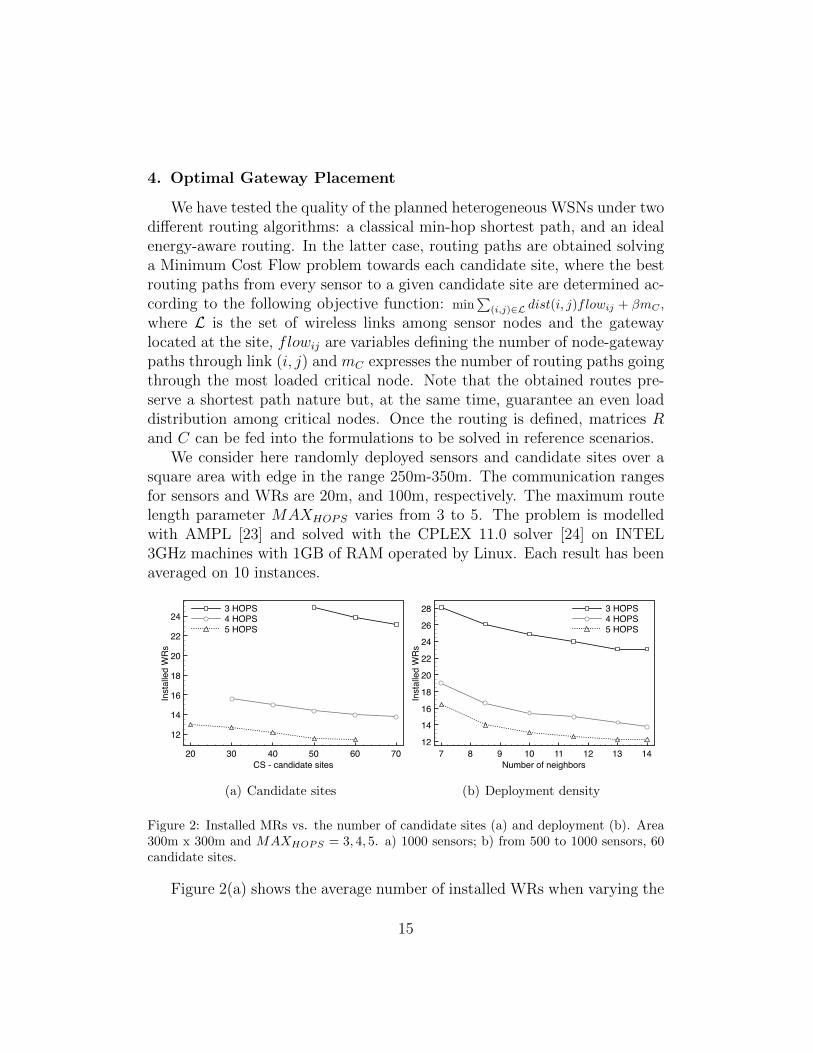
(a) Candidate sites (b) Deployment density

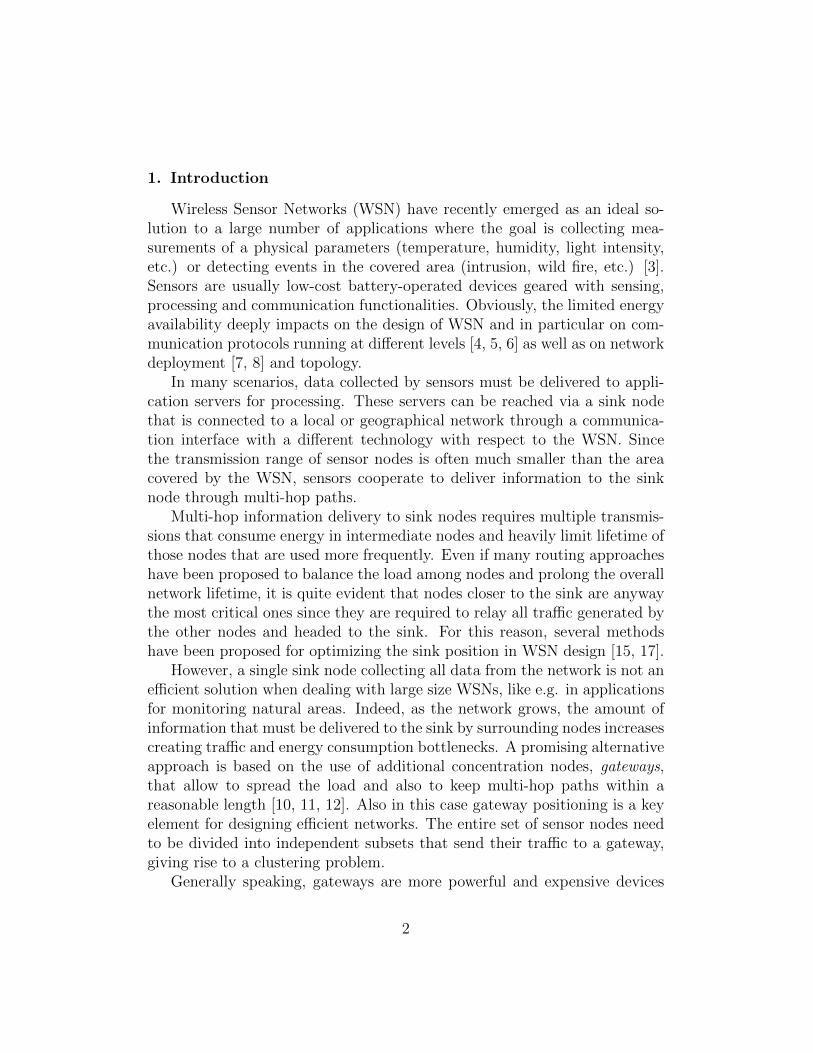
Figure 2: Installed MRs vs. the number of candidate sites (a) and deployment (b). Area300m x 300m and MAXHOPS = 3, 4, 5. a) 1000 sensors; b) from 500 to 1000 sensors, 60candidate sites.

Figure 2(a) shows the average number of installed WRs when varying the

15

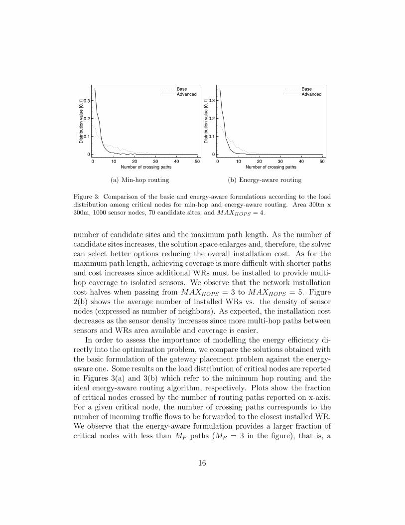
(a) Min-hop routing (b) Energy-aware routing

Figure 3: Comparison of the basic and energy-aware formulations according to the loaddistribution among critical nodes for min-hop and energy-aware routing. Area 300m x300m, 1000 sensor nodes, 70 candidate sites, and MAXHOPS = 4.

number of candidate sites and the maximum path length. As the number ofcandidate sites increases, the solution space enlarges and, therefore, the solvercan select better options reducing the overall installation cost. As for themaximum path length, achieving coverage is more difficult with shorter pathsand cost increases since additional WRs must be installed to provide multi-hop coverage to isolated sensors. We observe that the network installationcost halves when passing from MAXHOPS = 3 to MAXHOPS = 5. Figure2(b) shows the average number of installed WRs vs. the density of sensornodes (expressed as number of neighbors). As expected, the installation costdecreases as the sensor density increases since more multi-hop paths betweensensors and WRs area available and coverage is easier.

In order to assess the importance of modelling the energy efficiency di-rectly into the optimization problem, we compare the solutions obtained withthe basic formulation of the gateway placement problem against the energy-aware one. Some results on the load distribution of critical nodes are reportedin Figures 3(a) and 3(b) which refer to the minimum hop routing and theideal energy-aware routing algorithm, respectively. Plots show the fractionof critical nodes crossed by the number of routing paths reported on x-axis.For a given critical node, the number of crossing paths corresponds to thenumber of incoming traffic flows to be forwarded to the closest installed WR.We observe that the energy-aware formulation provides a larger fraction ofcritical nodes with less than MP paths (MP = 3 in the figure), that is, a

16

Table 1: Comparison among different problem formulations. Area 300m x 300m, 1000sensor nodes, 70 candidate sites, and MAXHOPS = 3.

Formulation Routing Installed Ave. load of Ave. load of MaxWR critical nodes overloaded nodes load

Basic Min-hop 13.8 4.47 10.75 30.5En-aware MP = 3 Min-hop 33.8 1.12 5.67 13.1En-aware MP = 3 En-aware 31.1 1.30 5.31 11.1En-aware MP = 0 Min-hop 42.0 0.79 6.89 19.0

larger fraction of not overloaded critical nodes. In addition, we can see howthe load distribution among critical nodes is more influenced by the problemformulation than by the routing algorithm. However, note that the use of theenergy-aware routing can help to reduce the number of heavy-loaded criticalnodes when using the basic formulation, that is, when gateway placementdoes not take the critical nodes’ load directly into account.

In Table 1 we summarize the average results for the number of installedWRs and the load of critical nodes with possible combinations of problemformulations and routing algorithms. We differentiate between the averageload of all critical nodes and the average load of overloaded nodes. The latterconsiders only the load (number of crossing paths) of critical nodes with anumber of crossing paths larger than the overload threshold (MP ), while theformer averages over all critical nodes.The last column of the table shows themaximum load experienced within the entire network. Note that the resultswith MP = 0 refer to the minimization of the total load of critical nodes,and not only the load of the overloaded ones.

Results confirm that solutions obtained with the energy-aware problemformulation have an average load on critical nodes that is substantially lowerthan the one of solutions with the basic formulation. However, this costsa higher number of installed WRs in order to evenly distribute the traffic.When the network is planned through the energy-aware formulation, the useof an energy-aware routing allows to reduce the number of installed WRs,however, it would seems it provides slightly worse solutions in terms of aver-age load. The reasons is that the energy-aware formulation does not aim atminimizing the average load of all critical sensors, but rather, it minimizesthe load of overloaded nodes, that is, ones with a number of crossing pathsabove the threshold MP . The table shows that the average load of overloadednodes, indeed, decreases. Finally, note that setting MP = 0 does not leadto a better solution. The average load of critical nodes is lower, but there

17

are overloaded critical nodes (with a number of crossing paths larger than 3)that are crossed by a high number of paths. Those nodes will soon exhausttheir batteries, disconnecting the network. In addition, this strategy resultsin a high number of installed WRs.

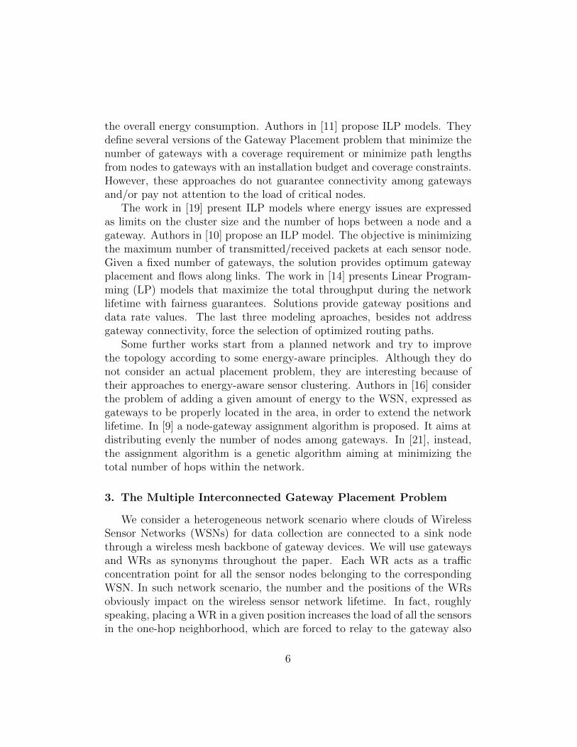
Figures 4(a) and 4(b) report two snapshots of planned networks withdifferent MAXHOPS. We reported the Voronoi diagrams representing theWSNs clouds around each installed gateway that allow to easily observe thatincreasing the MAXHOPS leads to larger clusters.

Figures 5(a), 5(b) and 6(a), 6(b) show the average and maximum loadof critical nodes when the budget formulation is applied with min-hop andenergy-aware routing, respectively. Note that as the degrees of freedom in-crease, that is, higher number of allowed path hops or higher budget, thequality of the solution increases. Indeed, the maximum load among criticalnodes decreases. The effect of using an energy-aware routing is a lower max-imum load, which is compensated by a slightly higher global average loadamong critical nodes.

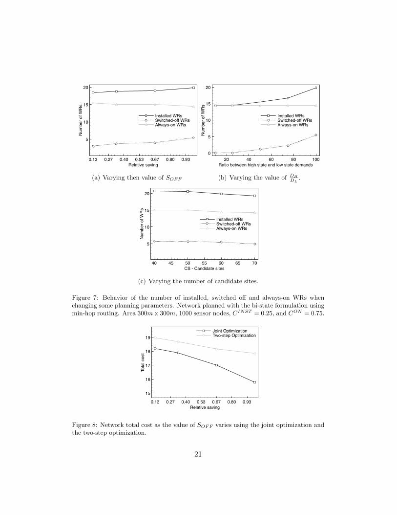
Finally we present results obtained from the bi-state formulation. Fig-ures 7(a), 7(b), and 7(c) show the main interesting results. They are ob-tained setting, where not differently stated, CINST = 0.25, CONTNET = 0.75,

SOFF =2

3, DL = 1, DH = 100, NCAP = 1500, and 60 available candidate

sites. Figures show the number of installed WRs, the number of WRs thatare switched off during the low state, and the ones that are kept on duringboth states.

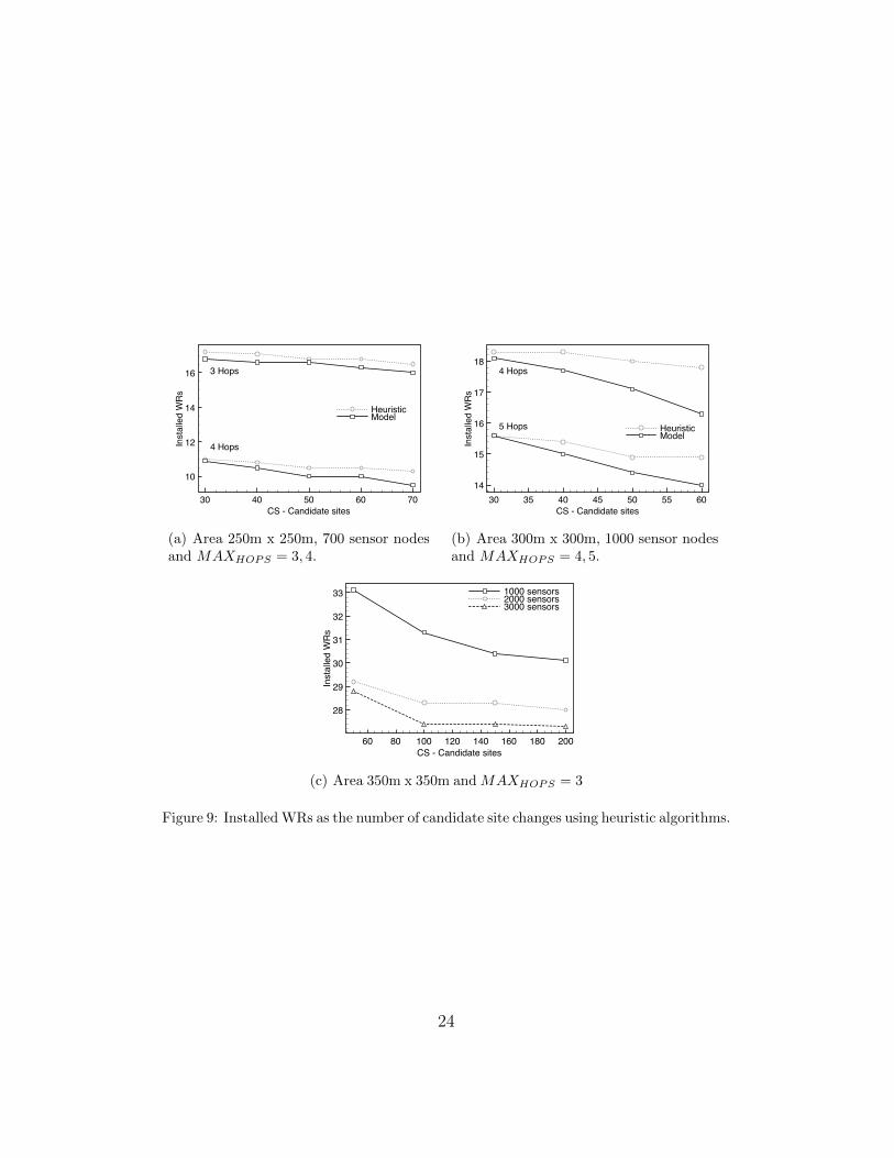
In Figure 7(a) the formulation’s behavior is analyzed when the savingvalue SOFF varies. Note that when the value increases, the number of in-stalled WRs increases. The number of WRs switched off during the lowstate increases as well, consequently, the number of always-on WRs slightlydecreases. As a result, the total cost of the network, that is, the value of theobjective function (21), reduces, as shown in Figure 8, black curve. This isdue to the fact that the higher saving when WRs are switched off allows tocompensate the costs of installing more WRs.

In order to assess the importance of this joint bi-state optimization, wehave run an alternative planning approach, which consists in sequentiallyapplying two optimization models. The first places WRs in order to minimizetheir number during the high state. The second, starting from the solutiongiven by the first one, aims at maximizing the number of deactivated WRsat the low state. Both models achieve their objectives taking into account

18

(a) MAXHOPS = 3.

(b) MAXHOPS = 5.

Figure 4: Network planned with the energy-aware formulation. Area 300m x 300m, 1000sensor nodes, 70 candidate sites.

19

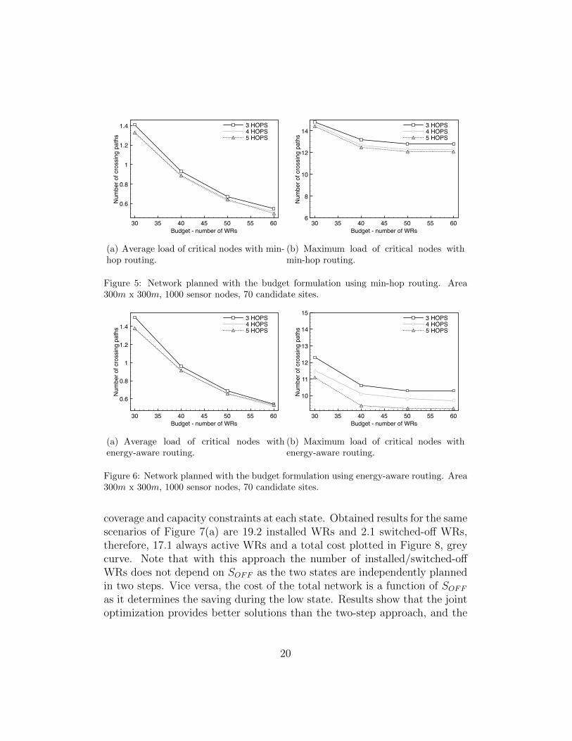
(a) Average load of critical nodes with min-hop routing.

(b) Maximum load of critical nodes withmin-hop routing.

Figure 5: Network planned with the budget formulation using min-hop routing. Area300m x 300m, 1000 sensor nodes, 70 candidate sites.

(a) Average load of critical nodes withenergy-aware routing.

(b) Maximum load of critical nodes withenergy-aware routing.

Figure 6: Network planned with the budget formulation using energy-aware routing. Area300m x 300m, 1000 sensor nodes, 70 candidate sites.

coverage and capacity constraints at each state. Obtained results for the samescenarios of Figure 7(a) are 19.2 installed WRs and 2.1 switched-off WRs,therefore, 17.1 always active WRs and a total cost plotted in Figure 8, greycurve. Note that with this approach the number of installed/switched-offWRs does not depend on SOFF as the two states are independently plannedin two steps. Vice versa, the cost of the total network is a function of SOFF

as it determines the saving during the low state. Results show that the jointoptimization provides better solutions than the two-step approach, and the

20

(a) Varying then value of SOFF (b) Varying the value of DH

DL.

(c) Varying the number of candidate sites.

Figure 7: Behavior of the number of installed, switched off and always-on WRs whenchanging some planning parameters. Network planned with the bi-state formulation usingmin-hop routing. Area 300m x 300m, 1000 sensor nodes, CINST = 0.25, and CON = 0.75.

Figure 8: Network total cost as the value of SOFF varies using the joint optimization andthe two-step optimization.

21

gap increases as the switch-off saving increases.Figure 7(b) shows the number of installed and switched off WRs as the

ratio between the traffic demand during the high state and the low statevaries. As we can see, when the ratio is low, actually no WR is turned off asthe traffic load reduction is not sufficient to require WR deactivations. Whenthe ratio increases, instead, more and more WRs are switched off during thelow state.

Finally, Figure 7(c) confirms that when the solver has more available siteswhere WRs can be placed, the quality of obtained solutions improves. Indeed,the number of installed WRs and WRs that are always active decreases asthe number of candidate sites increases.

5. Heuristic Algorithms

It is easy to show that the MIG-P problem is NP-hard since it containsthe Minimum Cardinality Set Covering problem as sub-problem. Even if wehave shown that the problem can be solved for reasonable size instances, wehave also designed heuristics to cope with large networks. We present firstan algorithm for the basic formulation of the MIG-P problem, and then weextend it to solve the energy-aware formulation.

Our heuristic approach is based on a continuous relaxation of the corre-sponding ILP model, and it can be summarized in the following three steps.

STEP 1 - Continuous relaxation. The ILP model (1)-(7) is solved relaxingthe integrality of variables yj (WR installation) and xij (node-WR assign-ment). Experimentally, we noted that about 60 − 70% of relaxed variablesare integer (with 10−9 precision), thus, we set the value of these variables to1 or 0. Other variables are rounded in the following step.

STEP 2 - Variable rounding. It consists of a greedy rounding over vari-ables yj:

• We generate an ordered list of candidate sites associated to fractionalvariables yj. The top-list candidate site is the one covering the largestnumber of sensor nodes.

• We scroll down the list starting from the top. For each site, we roundto 1 the associated variable until full coverage is achieved. At this pointthe coverage requirement is satisfied, but the connectivity one may benot.

22

• We generate a new ordered list of the candidate sites not yet considered:the first item is the candidate site with the smallest number of installedWRs in its neighborhood. In other words, the head of the list is themost isolated candidate sites.

• Again, we scroll the list rounding to 1 the associated variables, until theWMN is connected. At the end of this step coverage and connectivityrequirements are satisfied, thereby remaining fractional variables areset to 0. The result is an initial feasible solution to be refined in STEP3 removing WRS in excess.

STEP 3 - Refinement This step removes as many installed WRs as pos-sible without violating coverage and connectivity constraints. The installedWRs are ordered according to the non-increasing number of neighboringWRs. We scroll the list iteratively removing WRs. At each WR, if the so-lution is still feasible after its removal, we keep the new solution, otherwise,we re-insert the WR. When the end of the list is reached, the last feasiblesolution is the final one. Finally, the node-WR assignment is obtained run-ning the ILP model where variable yi are now parameters set according tothe above-described algorithm.

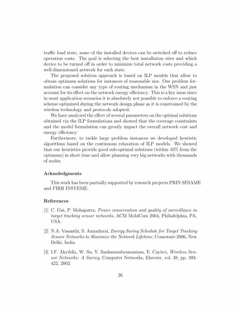
Figures 9(a) and 9(b) show the average optimality gap of the heuristicalgorithm under different numbers of sensor nodes and candidate sites. Asexpected, the quality of the heuristic solution slightly decreases when thesolution space increases (candidate sites number increases). However, thelargest gap is way below 10%.

As for the energy-aware formulation of the problem, the workflow of theheuristic does not change: STEP 1 solves the relaxed ILP model for theenergy-aware formulation, while STEP 2 and STEP 3 provide a feasible initialsolution. Only one further step, STEP 4, has been added to the previousframework.

STEP 4 - WR re-positioning The step that most significantly impacts onthe result of the algorithm is STEP 1, which fixes values of 60− 70% of theoverall variables. However, since assignment variables xij are relaxed duringSTEP 1, constraints (9) on the load of critical nodes cannot be properly eval-uated. Consequently, after STEP 3, we have solutions with a small numberof installed WRs, but with a poor quality in terms of energy consumption.The aim of this STEP 4 is to re-position installed WRs in order to decreasethe load of critical nodes. We iteratively perform the following move:

23

(a) Area 250m x 250m, 700 sensor nodesand MAXHOPS = 3, 4.

(b) Area 300m x 300m, 1000 sensor nodesand MAXHOPS = 4, 5.

(c) Area 350m x 350m and MAXHOPS = 3

Figure 9: Installed WRs as the number of candidate site changes using heuristic algorithms.

24

• We place each installed WR in one of the free candidate sites (yj =0) in its neighborhood. At each iteration, coverage and connectivityrequirements are verified. If the solution is feasible and it decreases theload of critical nodes (the second term of the objective function (8))with respect to the last feasible solution, then the new solution is kept.

This move is repeated until an improving solution cannot be found or amaximum number of iterations is reached.

We remark here that STEP 4 does not change the number of installedWRs which are just re-positioned in order to achieve a better load balancingamong critical nodes. The optimality gap of this approach, not reportedhere for the sake of brevity, has a very similar behavior to the one reportedin Figures 9(a) and 9(b). Again, the gap is upper bounded by 10% in all thecases under analysis.

We have tested the heuristic approaches also in large scale heterogeneousWSNs with 1000-3000 deployed sensor nodes and 50-200 available candidatesites in a square area 350m x 350m, which corresponds to a density of 10-30neighbors within the communication range.

The corresponding numerical results are shown in Figure 9(c) and confirmthe same performance trend highlighted by the optimal solutions.

6. Conclusion

In this paper we have proposed an optimization framework for the designof WSNs where gateways must be placed in the area and interconnectedwith the sink through the wireless links of a WMN. The resulting networkarchitecture is an heterogeneous multi-hop wireless networks where short-range low-rate links interconnect sensor nodes, while long-rage high-rate linkscreate a wireless backbone among gateways.

The objective is that of optimizing a tradeoff between the network in-stallation cost (the number of gateways if their installation cost is the same)and the energy consumption which is modelled considering the load of nodesdirectly connected to the gateways (critical nodes). The gateway selectionis subject to multi-hop sensor coverage constraints that guarantee that eachsensor can reach a gateway within a maximum number of hops. Moreover,the wireless network among gateways must be connected so as to allow themto deliver data to the sink.

We have also analyzed a scenario where the network operation consistsof two states: a low traffic load state and a high load one. During the low

25

traffic load state, some of the installed devices can be switched off to reduceoperation costs. The goal is selecting the best installation sites and whichdevice to be turned off in order to minimize total network costs providing awell-dimensioned network for each state.

The proposed solution approach is based on ILP models that allow toobtain optimum solutions for instances of reasonable size. Our problem for-mulation can consider any type of routing mechanism in the WSN and justaccount for its effect on the network energy efficiency. This is a key issue sincein most application scenarios it is absolutely not possible to enforce a routingscheme optimized during the network design phase as it is constrained by thewireless technology and protocols adopted.

We have analyzed the effect of several parameters on the optimal solutionsobtained via the ILP formulations and showed that the coverage constraintsand the model formulation can greatly impact the overall network cost andenergy efficiency.

Furthermore, to tackle large problem instances we developed heuristicalgorithms based on the continuous relaxation of ILP models. We showedthat our heuristics provide good sub-optimal solutions (within 10% from theoptimum) in short time and allow planning very big networks with thousandsof nodes.

Acknoledgments

This work has been partially supported by research projects PRIN SESAMEand FIRB INSYEME.

References

[1] C. Gui, P. Mohapatra, Power conservation and quality of surveillance intarget tracking sensor networks, ACM MobiCom 2004, Philadelphia, PA,USA.

[2] N.A. Vasanthi, S. Annadurai, Energy Saving Schedule for Target TrackingSensor Networks to Maximize the Network Lifetime, Comsware 2006, NewDelhi, India.

[3] I.F. Akyildiz, W. Su, Y. Sankarasubramaniam, E. Cayirci, Wireless Sen-sor Networks: A Survey, Computer Networks, Elsevier, vol. 38, pp. 393-422, 2002.

26

[4] I. Demirkol, C. Ersoy, F. Alagoz, MAC protocols for wireless sensor net-works: a survey, IEEE Communications Magazine, vol. 44, no.4, April2006, pp. 115–121.

[5] K. Akkaya, M. Younis, A survey on routing protocols for wireless sensornetworks, Ad Hoc Networks, Elsevier, vol. 3, no. 3, May 2005, pp. 325–349.

[6] L. Campelli, A. Capone, M. Cesana, E. Ekici, A Receiver Oriented MACProtocol for Wireless Sensor Networks, IEEE MASS 2007, Pisa, Italy,Oct. 2007.

[7] M. Cardei, Jie Wu Energy-efficient coverage problems in wireless ad-hocsensor networks, Computer Communications, Elsevier, vol. 29, no. 4,February 2006, pp. 413–420.

[8] E. Amaldi, A. Capone, M. Cesana, I. Filippini, Coverage planning ofWireless Sensors for Mobile Target Detection, IEEE MASS 2008, Atlanta(Georgia), Oct. 2008.

[9] G. Gupta, M. Younis, Load-Balanced Clustering of Wireless Sensor Net-works, IEEE ICC 2003, Anchorage (Alaska), May 2003.

[10] S. R. Gandham, M. Dawande, R. Prakash, S. Venkatesan, Energy Ef-ficent Schemes for Wireless Sensor Networks with Multiple Mobile BaseStations , IEEE GLOBECOM 2003, San Francisco, Dec. 2003.

[11] J.L. Wong, R. Jafari, M. Potkonjak, Gateway placement for Latency andEnergy Efficient Data Aggregation, IEEE LCN 2004, Tampa (Florida),Nov. 2004.

[12] A. Bogdanov, E. Maneva, S. Riesenfeld, Power-Aware Base Station Po-sitioning for Sensor Networks, IEEE INFOCOM 2004, Hong Kong, Mar.2004.

[13] K. Akkaya, M. Younis, M. Bangad, Sink Repositioning for EnhancedPerformance in Wireless Sensor Networks, Computer Networks, Elsevier,pp. 512-534, vol. 49, no. 4, 2005.

[14] H. Kim, Y. Seok, N. Choi, Y. Choi, T. Kwon, Optimal Multi-sink Posi-tioning and Energy-efficient Routing in Wireless Sensor Networks, IEEEICOIN 2005, Jeju Island, Feb. 2005.

27

[15] J. Pan, L. Cai, Y. T. Hou, Y. Shi, X. Shen, Optimal Base-Station Lo-cations in Two-Tiered Wireless Sensor Networks, IEEE Transactions onMobile Computing, vol. 4, pp. 458–473, 2005.

[16] Y. T. Hou, Y. Shi, H. D. Sherali, S. F. Midkiff, On Energy Provisioningand Relay Node Placement for Wireless Sensor Networks, IEEE Trans-actions on Wireless Communications, vol. 4, pp. 2579–2590, 2005.

[17] A. Efrat, S. Har-Peled, J. S. B. Mitchell, Approximation Algorithmsfor Two Optimal Location Problems in Sensor Networks, IEEE BROAD-NETS 2003, Boston, October 2005.

[18] J. Tang, B. Hao, A. Sen, Relay node placement in large scale wirelesssensor networks, Computer Communications, Elsevier, 29(4), pp. 490–501, Feb. 2006.

[19] B. Aoun, R. Boutaba, Clustering in WSN with Latency and EnergyConsumption Constaints, Journal of Network and Systems Management,Springer, vol. 14, no.3, pp. 415–439, 2006.

[20] W. Youssef, M. Younis, K. Akkaya, An Intelligent Safety-Aware Gate-way Relocation Scheme for Wireless Sensor Networks, IEEE ICC 2006,Istanbul, Turkey, June 2006.

[21] W. Youssef, M. Younis, Intelligent Gateways Placement for ReducedData Latency in Wireless Sensor Networks, IEEE ICC 2007, Glasgow,Scotland, June 2007.

[22] K. Akkaya, M. Younis, W. Youssef, Positioning of Base Stations inWireless Sensor Networks, IEEE Communications Magazine, vol. 45, no.4, pp. 96–102, April 2007.

[23] R. Fourer, D. M. Gay, and B. W. Kernighan, AMPL, A modeling lan-guage for mathematical programming, 1993.

[24] IBM ILOG Optimization - IBM ILOG CPLEX 11.0, http://www-01.ibm.com/software/integration/optimization/cplex/.

[25] M. Younis, K. Akkaya, Strategies and techniques for node placement inwireless sensor networks: A survey, Ad Hoc Networks, Elsevier, Volume6, Issue 4, June 2008, Pages 621-655.

28

[26] Y.B. Turkogullari, N. Aras, I.K Altinel, and C. Ersoy, Optimal Place-ment, Scheduling, and Routing to Maximize Lifetime in Sensor Net-works, Journal of the Operational Research Society, March 2009, doi:10.1057/jors.2008.187

29