Embed Size (px)
Citation preview

University of Nebraska - Lincoln University of Nebraska - Lincoln
DigitalCommons@University of Nebraska - Lincoln DigitalCommons@University of Nebraska - Lincoln
Computer Science and Engineering: Theses, Dissertations, and Student Research
Computer Science and Engineering, Department of
Winter 5-24-2009
Deployed Software Analysis Deployed Software Analysis
Madeline M. Diep University of Nebraska at Lincoln, [email protected]
Follow this and additional works at: https://digitalcommons.unl.edu/computerscidiss
Part of the Computer Engineering Commons, and the Computer Sciences Commons
Diep, Madeline M., "Deployed Software Analysis" (2009). Computer Science and Engineering: Theses, Dissertations, and Student Research. 1. https://digitalcommons.unl.edu/computerscidiss/1
This Article is brought to you for free and open access by the Computer Science and Engineering, Department of at DigitalCommons@University of Nebraska - Lincoln. It has been accepted for inclusion in Computer Science and Engineering: Theses, Dissertations, and Student Research by an authorized administrator of DigitalCommons@University of Nebraska - Lincoln.

DEPLOYED SOFTWARE ANALYSIS
by
Madeline Maretta Diep
A DISSERTATION
Presented to the Faculty of
The Graduate College at the University of Nebraska
In Partial Fulfillment of Requirements
For the Degree of Doctor of Philosophy
Major: Computer Science
Under the Supervision of Professor Sebastian Elbaum
Lincoln, Nebraska
May, 2009

DEPLOYED SOFTWARE ANALYSIS
Madeline Maretta Diep, Ph.D.
University of Nebraska, 2009
Advisors: Sebastian Elbaum
Profiling can offer a valuable characterization of software behavior. The richer the
characterization is, the more effective the client analyses are in supporting quality
assurance activities. For today’s complex software, however, obtaining a rich charac-
terization with the input provided by in-house test suites is becoming more difficult
and expensive. Extending the profiling activity to deployed environments can mit-
igate this shortcoming by exposing more program behavior reflecting real software
usage. To make profiling of deployed software plausible, however, we need to take
into consideration that there are fundamental differences between the development
and the deployed environments. Deployed environments allow for less overhead, pro-
vide less control for engineers to perform profiling adjustments, and generate high
volumes of information that may be overwhelming and often irrelevant to the client
analyses. These characteristics make existing techniques to support in-house profiling
inadequate for deployed environments.
In this dissertation, we describe the challenges in performing deployed software
profiling and propose deployed software analysis, i.e., a set of analysis techniques that
address these challenges and enable cost-effective deployed software profiling. Specif-
ically, we have developed and implemented techniques that can be applied to each of
the following stages of deployed software profiling: (1) before the software is deployed
to determine effective placements of the instrumentation probes that enable profiling;
(2) during deployment to drive the adjustments in profiling activity; and (3) after

deployment to efficiently process field data into meaningful and beneficial informa-
tion. Each proposed analysis technique is evaluated under a variety of deployment
settings to understand their efficiency and effectiveness trade-offs, and their impact
on the quality of dynamic analyses that consume the profiled field information. The
results suggest that the proposed analysis techniques can (1) reduce the profiling
cost to satisfy a variety of overhead constraints, (2) retain significantly more of the
gain provided by the field information when compared to control techniques, and (3)
increase the precision of dynamic analyses’s results by removing noise in field traces.

ACKNOWLEDGEMENTS
First, and foremost, I would like to express my highest gratitude to my advisor,
Sebastian Elbaum, for his generous guidance throughout my study. His technical
expertise, constant encouragement, and counsel are integral for the completion of
this work and for my growth as a graduate student. I feel very fortunate to have
him as an advisor.
I would also like to thank Myra Cohen and Matthew Dwyer for sharing their
valuable knowledge that have been crucial in the development of this dissertation;
and for providing their generous time to serve on my reading committee. I am also
grateful to Gregg Rothermel and David Rosenbaum who have kindly offer their time
and energy to serve on my dissertation committee and for their valuable insights.
My years as a graduate student at UNL would not be the same without the
presence of various members of the ESQuaReD research group, both past and
present. Their friendship, companionship, and their work ethics have often
comforted and inspired me. I am especially grateful to Suzette Person and to
Zhimin Wang who has directly contributed in MyIE study preparation.
Finally, I am thankful for my family, especially my husband Hao, who has patiently
supported, tolerated, and encouraged me in every aspects of my study; and my
parents and my sister for their unconditional love and constant push.
This work was supported in part by NSF CAREER Award 0347518.

5
Contents
1 Introduction 11.1 Motivation . . . . . . . . . . . . . . . . . . . . . . . . . . . . . . . . . 11.2 Contributions . . . . . . . . . . . . . . . . . . . . . . . . . . . . . . . 61.3 Organization of Dissertation . . . . . . . . . . . . . . . . . . . . . . . 10
2 Related Work on Deployed Analyses 112.1 Pre-deployment Phase . . . . . . . . . . . . . . . . . . . . . . . . . . 112.2 Deployment Phase . . . . . . . . . . . . . . . . . . . . . . . . . . . . 172.3 Post-deployment phase . . . . . . . . . . . . . . . . . . . . . . . . . . 222.4 Analysis across phases . . . . . . . . . . . . . . . . . . . . . . . . . . 26
3 Search-based Probe Distribution for Profiling Complex Properties0 283.1 A Motivating Example . . . . . . . . . . . . . . . . . . . . . . . . . . 303.2 Background, Definitions, and Approach . . . . . . . . . . . . . . . . . 34
3.2.1 Probe Distribution as a Sampling Problem . . . . . . . . . . . 343.2.2 Heuristic Search for Probe Allocation . . . . . . . . . . . . . . 36
3.3 Empirical Study . . . . . . . . . . . . . . . . . . . . . . . . . . . . . . 413.3.1 Study Setup . . . . . . . . . . . . . . . . . . . . . . . . . . . . 423.3.2 Independent Variables . . . . . . . . . . . . . . . . . . . . . . 453.3.3 Dependent Variables . . . . . . . . . . . . . . . . . . . . . . . 473.3.4 Threats to Validity . . . . . . . . . . . . . . . . . . . . . . . . 48
3.4 Results . . . . . . . . . . . . . . . . . . . . . . . . . . . . . . . . . . . 503.5 Conclusions and Future Work . . . . . . . . . . . . . . . . . . . . . . 56
4 Lattice-based Sampling for Profiling Path Properties0 584.1 A Motivating Example . . . . . . . . . . . . . . . . . . . . . . . . . . 604.2 Background, Definitions, and Approach . . . . . . . . . . . . . . . . . 69
4.2.1 Profiling Path Properties . . . . . . . . . . . . . . . . . . . . . 694.2.2 Sub-alphabet Properties and the Lattice . . . . . . . . . . . . 714.2.3 The Lattice of Sub-alphabet Properties . . . . . . . . . . . . . 724.2.4 Weighting Scheme of a Property Lattice . . . . . . . . . . . . 734.2.5 Sampling of Property Lattice . . . . . . . . . . . . . . . . . . 78
4.3 Path Property Profiling Infrastructure Support . . . . . . . . . . . . . 83

4.3.1 Lattices, Property Samples, and Program Variants . . . . . . . 844.3.2 Weighting Scheme . . . . . . . . . . . . . . . . . . . . . . . . 85
4.4 Empirical Study . . . . . . . . . . . . . . . . . . . . . . . . . . . . . . 874.4.1 Deployment Scenarios . . . . . . . . . . . . . . . . . . . . . . 884.4.2 Study Setup . . . . . . . . . . . . . . . . . . . . . . . . . . . . 914.4.3 Variables . . . . . . . . . . . . . . . . . . . . . . . . . . . . . . 964.4.4 Threats to Validity . . . . . . . . . . . . . . . . . . . . . . . . 97
4.5 Results . . . . . . . . . . . . . . . . . . . . . . . . . . . . . . . . . . . 1024.6 Conclusions and Future Work . . . . . . . . . . . . . . . . . . . . . . 121
5 Trace Normalization0 1235.1 A Motivating Example . . . . . . . . . . . . . . . . . . . . . . . . . . 1245.2 Background and Definitions . . . . . . . . . . . . . . . . . . . . . . . 130
5.2.1 Key Concepts: Commutative and Collapsible . . . . . . . . . . 1305.2.2 Approach Applicability and Trade-offs . . . . . . . . . . . . . 132
5.3 Trace Normalization Infrastructure Support . . . . . . . . . . . . . . 1355.3.1 State Identifier . . . . . . . . . . . . . . . . . . . . . . . . . . 1355.3.2 Decomposer . . . . . . . . . . . . . . . . . . . . . . . . . . . . 1365.3.3 Analyzer . . . . . . . . . . . . . . . . . . . . . . . . . . . . . . 1365.3.4 Trace Normalizer . . . . . . . . . . . . . . . . . . . . . . . . . 137
5.4 Empirical Study . . . . . . . . . . . . . . . . . . . . . . . . . . . . . . 1385.4.1 Study Setup . . . . . . . . . . . . . . . . . . . . . . . . . . . . 1395.4.2 Independent Variables . . . . . . . . . . . . . . . . . . . . . . 1415.4.3 Dependent Variables . . . . . . . . . . . . . . . . . . . . . . . 1425.4.4 Threats to Validity . . . . . . . . . . . . . . . . . . . . . . . . 144
5.5 Results . . . . . . . . . . . . . . . . . . . . . . . . . . . . . . . . . . . 1455.6 Conclusions and Future Work . . . . . . . . . . . . . . . . . . . . . . 152
6 Conclusion and Future Work 154
Bibliography 160

7
List of Figures
1.1 Summary of the research area. The proposed techniques are discussedin parenthesized chapters. Our preliminary work is annotated with a“P”. . . . . . . . . . . . . . . . . . . . . . . . . . . . . . . . . . . . . 7
3.1 Probe Distribution Strategies. Events that can be observed by eachdistribution are listed inside the parenthesis. . . . . . . . . . . . . . . 30
3.2 A snapshot of MyIE deployment website. . . . . . . . . . . . . . . . . 443.3 Identification of Call-Chains. . . . . . . . . . . . . . . . . . . . . . . . 503.4 Falsely Reported Call-Chains. . . . . . . . . . . . . . . . . . . . . . . 54
4.1 Integrated Constraint FSA–φ . . . . . . . . . . . . . . . . . . . . . . 634.2 Sub-alphabet FSA . . . . . . . . . . . . . . . . . . . . . . . . . . . . 644.3 Property Lattice for φ{c,o,r,w}. The shaded properties are the three
FSAs in Figure 4.3. . . . . . . . . . . . . . . . . . . . . . . . . . . . . 644.4 Weight Propagation for Lattice for φ{c,o,r,w} in the Case of Non-violated
Property. The weights of the property is represented as shades of grey.Properties marked by an * are profiled and properties marked by acheck mark were actually observed. . . . . . . . . . . . . . . . . . . . 66
4.5 Weight Propagation for Lattice for φ{c,o,r,w} in the Case of ViolatedProperty . . . . . . . . . . . . . . . . . . . . . . . . . . . . . . . . . . 68
4.6 Path Property Profiling Infrastructure . . . . . . . . . . . . . . . . . 834.7 Deployment Scenarios . . . . . . . . . . . . . . . . . . . . . . . . . . 894.8 Overview of Study Setup for Path Property Profiling . . . . . . . . . 914.9 The size of the sub-alphabets versus violation detection power of AS,
WS, NC, and TR. The size of a bubble indicates observation’s fre-quency. ∗ indicates a property in orig. . . . . . . . . . . . . . . . . . 104
4.10 The size of the sub-alphabets versus the cost of observing them in AS,WS, NC, and TR. ∗ indicates a property in orig. . . . . . . . . . . . 110
4.11 Violation Detection vs Number of Deployments . . . . . . . . . . . . 1124.12 Violation Detection vs Number of Variants (and Deployments) . . . . 1154.13 Rate of Violation Detection for Refinement With and Without feedback119
5.1 A snippet of NanoXML Program . . . . . . . . . . . . . . . . . . . . 1255.2 Trace Normalization approach steps applied to the example. . . . . . 126

5.3 Trace Normalization Infrastructure. . . . . . . . . . . . . . . . . . . . 1355.4 Fault Isolation Recall and Precision. . . . . . . . . . . . . . . . . . . 1465.5 Dynamic Change Impact Analysis Recall and Precision. . . . . . . . . 1485.6 Precision of the INS Techniques with vs Trace Pool Sizes. . . . . . . 1505.7 Precision of the Normalization Techniques vs Trace Length. . . . . . 151

List of Tables
2.1 Summary of sampling techniques. Our proposed techniques are markedwith a *. . . . . . . . . . . . . . . . . . . . . . . . . . . . . . . . . . . 14
3.1 Hypotheses . . . . . . . . . . . . . . . . . . . . . . . . . . . . . . . . . 423.2 Hill Climb Simulation Parameters . . . . . . . . . . . . . . . . . . . . . 473.3 p-values of the ANOVA Test . . . . . . . . . . . . . . . . . . . . . . . . 523.4 Homogenous groups of Cluster-based distribution . . . . . . . . . . . . . 53
4.1 SocketChannel properties as specification patterns and regular expres-sions. . . . . . . . . . . . . . . . . . . . . . . . . . . . . . . . . . . . . 61
4.2 Hibernate properties as specification patterns and regular expressions. 924.3 Summary of the four Hibernate clients. . . . . . . . . . . . . . . . . . 944.4 Summary of the sampling techniques. . . . . . . . . . . . . . . . . . . 118
5.1 Class score for fault isolation analysis performed on original traces. . 1275.2 Class score for fault isolation analysis performed on normalized traces. 1295.3 Segment Sets Information of NanoXML . . . . . . . . . . . . . . . . . 141

10
List of Algorithms
3.1 Greedy Algorithm for Probe-based Balanced Distribution . . . . . . 383.2 Hill Climb Algorithm for Probes Distribution . . . . . . . . . . . . . 394.1 General Property Sampling Strategy . . . . . . . . . . . . . . . . . . 82

1
Chapter 1
Introduction
1.1 Motivation
Software profiling aims to characterize a program’s behavior by observing its execu-
tion. The information collected through profiling is used to support quality assurance
activities such as to assess the adequacy of an existing testing effort through test cov-
erage measures, to characterize software usage to estimate its reliability [65], to isolate
faults [19, 40], to automatically construct patterns of software behavior [35, 87], to
dynamically infer program’s invariants [34], and to calculate change impact sets [49].
The effectiveness of software profiling in characterizing the program’s behavior
strongly depends on the thoroughness of the inputs provided to exercise the software.
Within the development environment, the profiled software is typically exercised by
a test suite prepared by the engineers. As software grows to be more complex in its
functionality, coupled with the increasing need for software to be highly configurable
and available on multiple platforms, it has become increasingly difficult for soft-
ware engineers to design a rich test suite that covers every possible usage scenario,
under all combinations of settings and configurations, especially with the limited

2
testing resources available in the development environment. To focus their testing
effort, engineers make assumptions about how the software will be used in deployed
environments, and their test suites reflect these assumptions. Inaccuracies in the
assumptions, however, may waste the testing effort and cause a degradation in the
quality and the reliability of the software, causing failures to occur in the deployed
environments even after the software is tested.
To address these limitations, researchers have proposed extending the software
profiling activity to deployed environments. Since the runtime information collected
at deployed sites reflects real user’s interactions with the program, it can be helpful
for engineers to validate their assumptions and to allocate resources for software im-
provement activities. Additionally, deployed sites may expose distinct configuration
settings and usage patterns that can yield vast and more diverse runtime information
than the in-house test suite. Integrating this information with the in-house quality
assurance activities can potentially increase the activities’ effectiveness.
Preliminary efforts to profile software after it has been deployed have been con-
ducted by development companies such as (1) Microsoft through its Window Error
Reporting (WER) tool [61] for various Microsoft products and for software and hard-
ware vendors interacting with Microsoft products through Window Quality Online
Services (Winqual) [57]; (2) Mozilla with its Quality Feedback Agent (also known as
Talkback) [66] and Breakpad for the more recent versions of Firefox and Thunderbird
[63]; and (3) Ubuntu, which utilizes an error reporting tool called Apport [86]. These
efforts mainly provide additional feedback when their software fails in the field; e.g.,
capturing heap stack snapshots when the program crashes or hangs. According to a
Microsoft developer, WER has reported more than 200 unique failures in Microsoft
Visual Studio, of which 78% were successfully fixed [50].

3
Analysis activities utilizing field information are not limited to fault isolation ac-
tivities. In an effort to construct better reliability models, for example, Microsoft
employs the Customer Experience Improvement Program (CEIP) [59]. The tool,
embedded in various products, tracks richer events than those of WER, such as com-
puter shutdown, restart, crashes, or driver install failures experienced by customers
who have opted into the program. It then uses the information to calculate fail-
ure rates and failure prevalence [68]. Moreover, research prototypes have also shown
that field information can be leveraged to assist various in-house testing activities to
further direct the testing resources by evaluating the assumptions made during the
testing activities [32], to create additional test cases [32, 33], or to provide additional
data for producing a richer understanding of how changes may impact users [69].
In order to be more efficient and effective, software profiling is enabled by various
analysis activities: analyses performed on the software to be profiled and analyses on
the runtime information obtained from software profiling. For example, static anal-
yses can be applied to the software to determine what program locations are to be
profiled, and field information can be processed to identify execution traces that con-
tain information needed by the engineers. Analysis activities to support profiling of
deployed software, later referred to simply as deployed software analysis, face some of
the same challenges as analyses used to support profiling in the in-house development
environment. In these cases, existing research efforts can also be applied to deployed
software analysis. However, there are some distinct differences between the in-house
environment and the field environment that give rise to additional challenges. Below,
we describe the challenges of profiling deployed software.
1. Overhead Constraints. Software instrumentation to enable software profil-
ing incurs runtime overhead. Past studies have reported that this overhead can
reach up to 970% of the execution time [9]. In contrast, Bodden et al. cited that

4
industrial companies are only willing to tolerate 5% runtime overhead from pro-
filing [9]. The overhead constraint due to instrumentation and profiling is even
more important in deployed environments than in the development environ-
ment as regular users will not be as tolerant to runtime overhead. Additionally,
overhead may also be incurred by the space required for information payloads
(information generated by profiling; e.g., execution traces, memory snapshots),
where the high volume of payloads may also translate into high storage costs.
The more instrumentation probes that are inserted and the more frequently
they are invoked, the higher the volume of the payloads. The overhead from
probe execution and the space required for the generated payloads limits the
amount of information that can be collected and prompts the need for strategic
placement and invocation of the instrumentation probes.
2. Enormous Amounts of Data to Process. The payload volume generated
by profiling can overwhelm engineers as they sift through the data to find the
relevant information. When isolating faults, for example, engineers may want
to look at all of the failed runtime information that may potentially relate to
such faults. However, as identified by Podgurski and Yang, “checking program
behavior is one of the most time-consuming parts of testing” [76]. This problem
is aggravated when it comes to deployed environments because executions in
deployed environments tend to be redundant (users tend to exercise common
functionalities of the program) and can involve long executions that include
multiple program functionalities. For example, a site for searching and viewing
crash reports submitted through Mozilla’s Breakpad [64] shows that about 1100
reports related to Firefox were received in one hour just for its top 100 errors
(categorized through their stack signatures). Such pools of data are filled with
noise in the form of irrelevant or duplicated information.

5
3. Overwhelming Amounts of Data to Transfer. The transfer of information
from the deployed sites to the development company consumes computation
bandwidth and storage resources. For the deployed sites, data transfer implies
additional computation cycles to marshal and package the data, bandwidth
to perform the transfer, and a likely increase in the runtime overhead. In
one of our previous studies, we found that a 41K LOC program deployed with
instrumentation to capture the basic blocks executed, the menu’s item traversed,
the basic program inputs, and the program’s initial settings and configurations
transferred approximately 240KB data per deployed site per day [24]. For an
organization with thousands of deployed software instances trying to capture
richer data, this can clearly become a bottleneck. This suggests that there is an
important need to be efficient when transferring the field data to the company,
for example, by identifying and transferring only the unique information at each
site.
4. Shifting of Profiling Target. Feedback received from the field may shift the
engineers’ interest to a different analysis or to a different part of the software
than what was originally intended. Empirical studies have revealed that, if the
instrumentation probes remain unchanged, profiling returns new information
in an inverse exponential rate over time [17, 32]. Furthermore, profiling de-
ployed software relies on making assumptions about the users’ behaviors and
estimations about profiling cost when allocating the instrumentation probes
to the users. Unanticipated changes in the users’ behaviors may break those
assumptions, rendering existing probes useless and generating inaccurate esti-
mates of the profiling cost which in turn may cause the overhead constraints
to be violated. These issues prompt the need for analyses that allow engineers
to continuously assess the profiling process to improve its effectiveness and ef-

6
ficiency in the presence of changes.
5. Privacy and Security. Profiling deployed software raises issues of privacy and
security. While these are important issues which may hinder the effectiveness
of the analysis activities due to the hesitation on the users’ part to participate
or the risk in collecting and maintaining such critical data, this topic is outside
the scope of this dissertation.
1.2 Contributions
We have developed a set of deployed software analysis techniques to address these
challenges and to increase the cost-effectiveness of profiling deployed software. Fig-
ure 1.1 provides an overview of how we have approached the development of such
techniques. We categorized the analysis techniques along three main threads: (1)
analyses that occur in the pre-deployment stage of the profiling process, (2) analyses
that occur during deployment, and (3) analyses that occur in the post-deployment
phase. This division corresponds to the three phases in the lifecycle of deployed pro-
gram profiling, which we describe in greater detail in Section 2. Approaches marked
by a “P” in Figure 1.1 were developed as part of my Master’s thesis (also part of [32])
and will be summarized in Chapter 2.
Pre-Deployment
At the pre-deployment phase, we are concerned with the challenge of strategically
placing probes to reduce the overhead incurred by profiling complex state
and path properties. Complex properties refer to properties that require the inser-
tion and invocation of probes in multiple program locations to produce meaningful
information. Profiling state properties requires instrumentation for capturing val-

7
Deployed Software Analysis
Pre-Deployment During Deployment Post-Deployment
Strategic probe placement
Balance profiling cost and value
Leverage field data
Profile complex state properties through a
search-based sampling technique
(Ch. 3)
Profile path properties through
sampling of a property lattice
(Ch. 4)
Identify and normalize irrelevant variations
(Ch. 5)
Generate test cases
(P)
Area
Remove trace noise
Trigger transfers
(P)
Challenge
Technique
Sub-Area
Figure 1.1: Summary of the research area. The proposed techniques are discussed inparenthesized chapters. Our preliminary work is annotated with a “P”.
ues (e.g., predicates, program variables, program blocks, methods traversed) at spe-
cific program locations. Profiling path properties (also known as temporal or types-
tate properties) requires instrumentation for verifying proper sequencings of program
events (e.g., method calls on an API).
In this dissertation, we have developed two sampling-based techniques to dis-
tribute instrumentation probes across deployed sites for profiling complex properties
that can be tuned to satisfy an overhead budget. Our work improves on the previ-
ous sampling-based approaches for deployed program profiling (discussed in detail in
Section 2.1) by:
1. Comprehensively defining probe distribution as a sampling problem with multi-
ple sampling dimensions (e.g., time, probe locations, deployed sites, properties)
and sampling constraints (e.g., overhead budget, number of program variants,
number of deployed sites). Moreover, we were the first to optimize the probe dis-

8
tributions by considering the relation between the distributed instrumentation
probes across program variants.
2. Targeting the overhead cost caused from profiling path properties associated
with method invocations (existing techniques for monitoring path properties
focus on reducing cost by sampling the allocated objects). Our technique was
the first to leverage the semantic structures of path properties to (1) enrich
the space of sampling, providing a pool of path properties where each property
constrains a different subset of method calls, (2) order the properties as a lattice
where a path property subsumes another path property if its set of method calls
is a superset of the other property’s method calls, and (3) drive the sampling
strategy to select path properties with varied detection capabilities by leveraging
the fact that a subsumed property always has less violation detection capability
than its subsuming property.
During Deployment
At the deployment phase, we are concerned with balancing the cost of profiling
with the return value of the profiled information by providing only the infor-
mation that may be of interest to the engineers. In my Master’s thesis, I explored the
opportunity to mitigate the cost of profiling, by reducing the number of unnecessary
field transfers through a set of triggering techniques (also in [32]).
In this dissertation, we look at another opportunity to improve the return value of
the profiled information through iterative profiling. We extend the work of profiling
path properties and develop an analysis technique that leverages feedback from the
field (e.g., observed properties) to refine the profiling process. Our technique is similar
to other techniques that remove or decrease the rate of invocations of instrumentation
probes on the program locations that have been observed sufficiently. However, our

9
technique is especially intended for profiling path properties, which enables us to:
1. Leverage the ordering relations between path properties that compose the sam-
pling space (lattice) to make inferences about the value of properties that were
not directly observed. For example, if a property is violated, then any of its
subsuming properties are also violated. Similarly, if a property is observed, then
any of its subsumed properties are also observed.
2. Prune the sampling space by discarding path properties that are unlikely to be
observed due to the specific deployed site’s usage characteristics. Our technique
utilizes the site-specific feedback to determine unlikely method calls and the
corresponding path properties that constrain them to avoid instrumenting for
those properties.
Post-Deployment
At the post-deployment stage, we aim to provide support in managing and pro-
cessing field information. Previously, we have quantified the potential benefit of
leveraging field information, developed techniques to generate test cases from field
data, and evaluated the gains provided by those test cases [32].
In this dissertation we focus on the challenge of removing redundant and noisy
information within execution traces to improve the precision of the dynamic analy-
ses that consume them. We have developed techniques to analyze execution traces
for patterns of event sequences that can indicate irrelevant differences between (and
within) traces with respect to properties inferred by the client analyses. Our tech-
niques are built upon existing work in trace comparisons [13, 22, 39, 51] where we
use abstractions of program behavior to determine if two traces are the same. Our
techniques contribute to this research area by:

10
1. Identifying variations in event sequences that may contribute to imprecision in
client analyses, and normalizing those variations. More concretely, our tech-
niques rely on heuristics to identify events whose orderings or repetitions do
not affect the semantics of the trace from the perspective of a client analysis.
2. Introducing the notion of trace segmentation where an execution trace is sys-
tematically decomposed into smaller units. This enables a more precise analysis,
by operating on trace segments instead of whole traces, and is independent of
the length of the traces.
For each of the proposed techniques across the three phases, we perform an empir-
ical study to evaluate their performance through real deployments, simulation, and
case studies. In these studies, we focus on the trends and the trade-offs between the
cost and the effectiveness of the analysis techniques.
1.3 Organization of Dissertation
The remainder of this dissertation is organized as follows. Chapter 2 defines the three
stages in the lifecycle of profiling deployed software, categorizes the analysis activities
that may be performed at each stage, and describes their corresponding related work.
Chapters 3, 4, and 5 present the analysis techniques we have developed to target
the challenges described previously for each stage of the profiling lifecycle. In each
chapter, we first describe our motivation through an example, explain the concepts
and background of the technique, and introduce the techniques and their required
infrastructure. Then, we pose the research questions, the study setup for evaluating
the technique, and the threats to the study’s validity. Finally we present the results,
conclusion, and possible future work for each technique. Chapter 6 provides the
overall conclusions for this dissertation and suggests areas for further study.

11
Chapter 2
Related Work on Deployed
Analyses
The lifecycle of the profiling process of a deployed program can be viewed as a con-
tinuous cycle consisting of three phases: (1) pre-deployment, (2) during deployment,
and (3) post-deployment. In this section, we categorize deployed program analyses
according to the phases in which they support the profiling activity, and describe
them. When relevant, we also provide a more detailed description of our preliminary
work (the boxes that are marked with “P” in Figure 1.1).
2.1 Pre-deployment Phase
The first phase is the pre-deployment phase, where engineers prepare the software
to be deployed. In this phase, the engineers define the information of interest and
insert instrumentation probes into the software to obtain it. Many infrastructures are
available for convenient program instrumentation. For example, Javassist, BCEL, and
ASM are libraries that can be utilized to instrument Java programs at the byte code

12
level [16, 20, 73]; CCI is an instrumentation tool targeting Ansi C [82]; Dyninst is an
API for C++ that allows runtime modification of a program for probe insertion [14];
Pin is a tool for runtime probe insertion into Linux binary executables [75]; Misurda
et al. propose a framework that allows for insertion and removal of instrumentation
probes depending on the profiling demand [62]; and Aspect Oriented Programming
(AOP) is a programming paradigm that allows profiling tasks to be treated as a
crosscutting concern, separating the instrumentation codes to perform profiling from
ones that perform the program’s actual functionality [37].
The profiling activity may incur significant overhead due to the invocations of
the instrumentation probes. Analyses are performed in the pre-deployment phase to
determine the best placement or the rate of probe executions that allows for reduc-
tion in the overhead (runtime and payload), while still capturing the information of
interest. Existing techniques that address this problem can generally be categorized
in two groups: (1) lossless and (2) lossy techniques.
Lossless analysis techniques aim to reduce profiling overhead by identifying redun-
dant program locations and excluding them from being profiled, hence reducing the
number of probes while causing no loss in the generated information. Redundancy can
originate from two sources. First, profiling program locations that do not reveal new
or meaningful information would produce redundant information. Such redundancy
can be eliminated, for example, by identifying residual program locations, i.e., ones
that have not been exercised during in-house testing, and allocating enough probes
just to profile them [74], or by dynamically removing probes after their associated
properties are observed [17, 83]. Similarly, when profiling for violations detection in
path properties, researchers have employed sophisticated static analyses to identify
safe areas in the program where violations could not occur, eliminating the need to
place the probes in these locations [9, 11, 30]. The second source of redundancy

13
comes from profiling properties that can be inferred from the observation of other
properties. Techniques have been proposed, for example, to leverage programs’ call
graphs to identify inferrable probes to profile block coverage [1], whole program path
[7], and a subset of procedural acyclic paths [3].
Lossless techniques, however, may not be sufficient to reduce the profiling overhead
to satisfy the stricter overhead constraints of deployed environments. For a more
aggressive overhead reduction, but with a potential loss in the obtained information
and the introduction of false positives in the analyses, lossy techniques based on many
forms of sampling are necessary. Sampling-based approaches select a subset of the
instrumentation probes to be inserted into a deployed program variant or a subset
of the probes to be invoked in a program run, subjecting each program execution to
a much smaller overhead. Sampling leverages the opportunities offered by deployed
environments, i.e., the availability of multiple deployed sites and program executions,
to profile only a subset of the program behavior exposed at each site or execution,
but still collectively approximate how a program is exercised overall.
The sampling techniques that have been proposed can be categorized according to
the dimension over which the sampling is performed, the type of profiled properties
(e.g., simple - require instrumentation probes that are independent of each other to
generate meaningful information such as to profile state coverage or variable values;
or complex - require instrumentation probes that are dependent to each other such as
to profile call-chains or path properties), and when sampling occurs (online - during
program execution; or offline - probes locations are determined and fixed in-house).
In Table 2.1, we summarize and categorize some of the existing sampling techniques.

14
Ref Description Dimension Properties Performed[36] Estimates the execution time spent on
each program routine by sampling theprogram counter’s value at fixed inter-vals.
Time Simple Onlinea
[4] Creates duplicates of code segments thatcontain instrumentation probes and sam-ples between instrumented and non-instrumented code.
Profiled prop-erties
Simple Online
[72] Breaks the profiling task into smallerunits and distributes the unit across de-ployed instances.
Deployed sites,Profiled tasks
Complex Offline
[52] Samples across the invocations and val-ues of program predicates using Bernoullidistribution and statistically ranks thepredicates on their likelihood to cause afailure.
Profiled prop-erties
Simple Online
[32](P) Stratifies probes according to their classlocations and samples across the strata.
Deployed sites,Profiled prop-erties
Simple Offline
[23]* Utilizes a search heuristic to distributeprobes across variants optimally relativeto a function that favors balancing andpacking of probes in a distribution.
Deployed sites,Profiled prop-erties
Complex Offline
[10] Identifies and samples across regions ofprogram behavior that correspond to in-dependent instances of path property.
Deployed sites,Profiled prop-erties
Complex Offline
[5] Samples across object instances and pro-file relevant method calls that are per-formed on the sampled objects.
Profiled prop-erties
Simple,Complex
Online
[28]* Composes an integrated property froma set of path properties, breaks it downinto a set of sub-properties, and leveragesvarious structure of the sub-properties tosample across them.
Deployed sites,Profiled prop-erties
Complex Offline
aNote that, although the online sampling strategies shown in Table 2.1 inherently determinewhich probes are invoked during a run (i.e., during deployment), the analysis is done during thepre-deployment phase to determine the sampling parameters. Because of that, we categorize onlinesampling techniques under pre-deployment.
Table 2.1: Summary of sampling techniques. Our proposed techniques are markedwith a *.

15
Our Preliminary Work – Stratified Sampling
In my Master’s thesis I introduced a simple sampling technique, stratified sampling,
to determine the placement of instrumentation probes for profiling simple properties.
The main idea of stratified sampling is to group the population of instrumentation
probes according to a similarity criterion and then sample across the sub-populations
(groups or stratum), where each probe belongs to exactly one strata. If the strat-
ification process generates subsets of populations that are somewhat homogenous,
stratified sampling can yield a sampled set containing probes that are representative
of the probe population.
Sampling is repeatedly performed across strata in proportion to the size of the
strata’s populations to create n sets of instrumentation probes, each containing H
probes, to be inserted into n program variants. There is a trade-off between the
values of H and n. Maintaining H constant while increasing n provides more and
maybe redundant observations across variants. The technique offers the opportunity
to leverage this overlap to reduce H, reducing overhead at each deployed site by
collecting less data while compensating by profiling more deployed instances (trading
more n for less H).
We evaluated the performance of stratified sampling. To do this, we fully instru-
mented1 a text-based e-mail application for Unix called Pine and deployed it to 30
users for a period of 14 days. Prior to deployment, a test suite consisting of 288
test cases was developed where it covered 61% of the program’s functions. The over-
head of running the instrumented program variant was approximately 14%. Then we
simulated our stratified sampling technique over the obtained field information.
We measured the performance of the stratified sampling and compared it to the
1All of the instrumentation probes are inserted into the deployed program. We refer to this asthe full technique.

16
full technique (all program blocks profiled). We evaluated the impact of varying the
number of program variants on the additional coverage gained and the number of
probes executed (overhead). Stratified sampling reduced the runtime overhead from
52% up to 98% when compared to full. The least aggressive stratified sampling
technique – stratified sampling to generate 2 program variants where each variant
contains 50% of the probes – provided 8% of coverage gain (1% less coverage gain
than was provided by full) with 7% runtime overhead. Our most aggressive stratified
sampling provides 3% coverage gain with only 0.3% runtime overhead. A more de-
tailed description of the empirical study, the analysis of the results, and the discussion
of the threats to validity can be found in the paper [32].
Our Proposed Techniques
In this dissertation we present two sampling techniques to improve upon initial work
for profiling complex properties. Following the characterizations used in Table 2.1,
our sampling approaches (1) perform sampling of sets of dependent probes, associated
with the complex properties, across the deployment sites; that is, we generate program
variants containing a subset of the probes that are then deployed to one or multiple
sites; (2) determine the probe locations offline which removes the need of having
additional analysis to perform the sampling at run-time; and (3) enable profiling
of complex properties that is capable of producing sound reports given that certain
conditions are met. In Chapter 3 we show one possible situation that breaks this
condition and introduce false positives in the analysis. In Chapter 4 we discuss one
necessary condition to ensure sound violation detection reports.
Two of the techniques listed in Table 2.1 [10, 72] share the same characteristics as
our approaches. We now discuss their differences compared to our techniques. The
first technique, developed by Orso et al. [72], enables profiling of complex properties

17
aimed to address the overhead problem. However, it provides only a mechanism to
distribute a set of given properties across sites, not to ensure that the overhead bound
can always be reached. The second technique for profiling path properties, proposed
by Bodden et al. [10], identifies groups of object allocation sites that correspond to
independent instances of a path property which can be used to define the sampling
space. The technique reduces the number of allocated objects that need to be profiled.
However, even when a single object is profiled, the number of method calls performed
on the object can cause the profiling overhead to be excessive. Our proposed approach
mitigates this problem and it is orthogonal to the approach of Bodden et al. [10]. Our
technique generates a pool of related path properties and leverages the properties’
relations to drive the sampling selection strategy. As we briefly discuss in Section
2.2, the properties’ structures can be used during deployment to refine the selection
of path properties to profile. We present our techniques in Chapters 3 and 4.
2.2 Deployment Phase
The second phase of profiling occurs during deployment itself. In this phase, a connec-
tion between the sites in which the software is deployed and the development company
is established. Through this connection, the information related to a user’s execution
can be transferred back from the deployed site to the company. The company may
also provide feedback, bug fixes, and adjustments to the profiling activity at the de-
ployed sites. During deployment, it may also become necessary to tailor the probe
allocation, especially when the cost of profiling begins to outweigh its benefit, such
as when no new information is obtained though profiling still consumes resources.
Deployed software analyses are needed to support the profiling process during the
deployment phase in at least two ways: (1) to allow efficient transfer of field data and

18
(2) to tailor the profiling process by adjusting the probe locations.
Efficient Transfer. Transferring field information from the deployed sites to the
development site must be efficient with respect to the size and frequency of transfers.
Many techniques have been proposed to apply different encodings to the execution
traces to decrease their physical size without causing a loss in the contained informa-
tion [38, 79], requiring less resources to store and transfer the runtime data. Another
set of techniques addresses this problem by transferring only the information of inter-
est to the engineers [32, 42]. Most of the commercial reporting tools, such as WER
and Breakpad, collect and send the gathered information only when a fatal failure
occurs [60, 63].
Several research efforts leverage the notion of anomalous behavior to trigger field
data transfer. Employing anomaly detection implies the existence of a baseline be-
havior that is considered nominal or normal. When targeting deployed software, the
nominal behavior can be defined by what the engineers know or understand from the
program. Departure from the nominal behavior interests engineers because it may
reveal new behavior or manifested failures in the program execution. Such triggering
techniques require the definition of three main components: (1) a model to charac-
terize a program’s behavior, (2) a set of the model’s instantiations that represents
the nominal behaviors, and (3) a tolerance to deviations from the nominal behavior.
Many different models have been proposed: event patterns, which are employed by
EDEM to collect deviating user-interface feedback [42], Probabilistic Calling Context
(PCC), a unique value calculated through a probabilistic function representing the
sequence of method calls that lead to a program location [12], and operational profile,
program invariants, and Markov models, which we have explored in our previous work
[32] and will discuss in greater detail later in this section.
Tailored Profiling. Instrumentation probes are often allocated to the deployed
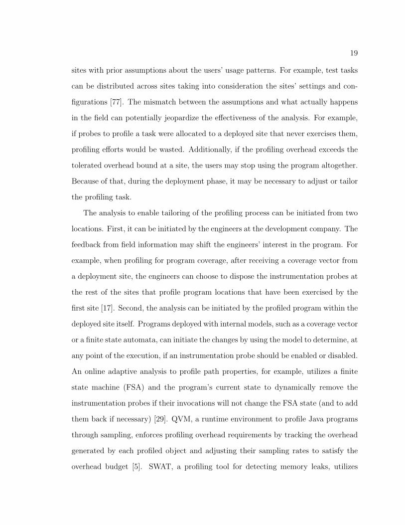
19
sites with prior assumptions about the users’ usage patterns. For example, test tasks
can be distributed across sites taking into consideration the sites’ settings and con-
figurations [77]. The mismatch between the assumptions and what actually happens
in the field can potentially jeopardize the effectiveness of the analysis. For example,
if probes to profile a task were allocated to a deployed site that never exercises them,
profiling efforts would be wasted. Additionally, if the profiling overhead exceeds the
tolerated overhead bound at a site, the users may stop using the program altogether.
Because of that, during the deployment phase, it may be necessary to adjust or tailor
the profiling task.
The analysis to enable tailoring of the profiling process can be initiated from two
locations. First, it can be initiated by the engineers at the development company. The
feedback from field information may shift the engineers’ interest in the program. For
example, when profiling for program coverage, after receiving a coverage vector from
a deployment site, the engineers can choose to dispose the instrumentation probes at
the rest of the sites that profile program locations that have been exercised by the
first site [17]. Second, the analysis can be initiated by the profiled program within the
deployed site itself. Programs deployed with internal models, such as a coverage vector
or a finite state automata, can initiate the changes by using the model to determine, at
any point of the execution, if an instrumentation probe should be enabled or disabled.
An online adaptive analysis to profile path properties, for example, utilizes a finite
state machine (FSA) and the program’s current state to dynamically remove the
instrumentation probes if their invocations will not change the FSA state (and to add
them back if necessary) [29]. QVM, a runtime environment to profile Java programs
through sampling, enforces profiling overhead requirements by tracking the overhead
generated by each profiled object and adjusting their sampling rates to satisfy the
overhead budget [5]. SWAT, a profiling tool for detecting memory leaks, utilizes

20
an adaptive profiling scheme that adjusts the instrumentation points’ sampling rates
to be inversely proportional to their execution frequencies [40]. These efforts allow
in-house or on-the-fly adjustments to eliminate unnecessary or harmful profiling.
Our Preliminary Work – Triggering Techniques
To address the need for efficient transfer of field data, we have developed trigger-
ing techniques to initiate field data transfer when anomalous program behavior is
detected. We define a triggering approach as follows. Given a program p, a set of
properties to profile Prop, an in-house characterization of those events Prophouse,
and a tolerance to deviations from the in-house characterization ProphouseTolerance,
this technique generates a program variant vi with additional instrumentation to pro-
file events in Prop, and a detection algorithm to identify when field behavior Propfield
deviates from [Prophouse ± ProphouseTolerance]. When such deviation is detected, field
data is transferred to the development company. We consider three triggering tech-
niques corresponding to how Prophouse is characterized. We also consider whether
feedback from the transferred field data is utilized to refine the Prophouse.
The first technique uses operational profiles and triggers a transfer when there is
a departure from the program’s existing operational profile. An operational profile
consists of a set of operations and their associated probabilities of occurrences [65]
and can be used to guide the test suite generation process or the allocation of testing
resources. We implement the operation profile as a vector of probabilistic values where
we construct one vector to represent each user’s usage patterns. The ProphouseTolerance
is instantiated in terms of the minimum and maximum values, or average and standard
deviations of a set of operational profiles vectors.
The second technique triggers a transfer when an existing program invariant is
violated. Program invariants can be thought of as assertions on the program spec-

21
ifications that have to hold true at any point in the program’s execution. In this
technique, we set ProphouseTolerance = 0.
The third technique uses Markov models to characterize the field behavior into
three groups: pass, fail, or unknown. One specific encoding of Markov models is in the
form of an n by n matrix, where n is the number of profiled program locations. Each
cell (i, j) in the matrix represents the probability that an observation of location i
is followed by an observation of location j. Engineers construct Markov models from
passing or failing execution traces and use them to classify other execution traces
[13]. Two models match (i.e., are successfully classified as passing or failing) if their
Hamming distance does not exceed a threshold value ProphouseTolerance (i.e., there are
less than ProphouseTolerance differences between their cell’s values). A field trace is
transferred if it is classified as a failing execution or as unknown.
We performed an empirical study using Pine to evaluate the impact of each trigger-
ing technique on the amount of coverage, fault detection, and correctness of inferred
invariants. To obtain the set of nominal behaviors, we selected a percentage of users
of the instrumented Pine and utilized their usage information along with the in-house
test suite to construct sets of operational profiles, invariants, and Markov models.
All anomaly detection techniques reduced, to different levels, the number of transfers
required by the full technique. Such reduction, however, can sacrifice the potential
gains in coverage and fault detection, or infer less accurate invariants. The triggering
technique using operation profiles offered the most aggressive reduction capabilities
(up to 98% reduction is achieved when we use half of the users as a training set)
but could lead to the detection of only 22% of the faults. Such a technique would fit
in settings where data transfers are too costly, only a quick exploration of the field
behavior is possible, or the number of deployed instances is large enough that there
is a need to filter much of the data. The invariant based detection technique offered

22
a more detailed characterization of the program behavior, which results in a 46%
transfer reduction but allows the detection of 67% of the faults. Markov-based tech-
niques provided the best combination of reduction (up to 36%) and fault detection
gains (99% of faults detected), but their on-the-fly computational complexity may
not make them viable in all settings.
Our Proposed Technique
We extend our sampling approach for profiling path properties to enable the refine-
ment of the path properties being profiled. The changes in what path properties to
profile can be customized by the engineers at the development company by analyzing
the properties observed and violations detected in the field. Employing the subsum-
ing relations within our lattice of properties, we can propagate what we learn from
observing a property to other related properties. Our approach uses an intuition
similar to the work of SWAT [40], where we decrease the chance of a property being
sampled after it has been observed in an execution. Our technique differs from SWAT
in that we also consider site-specific characteristics to drive the sampling process at a
deployed site to avoid profiling path properties that cannot be observed in that site.
The technique is presented in Chapter 4.
2.3 Post-deployment phase
The last phase of profiling occurs within the development environment. In the post-
deployment phase, the information from the field is managed and analyzed to refine
in-house testing and dynamic analyses to improve software quality and future profiling
activities. The sheer amount of information obtained from the field prompts the need
for analysis techniques that can aid in managing such information. Additionally,

23
field information may be redundant and contain irrelevant information. Deployed
software analysis supports profiling during the post-deployment stage by (1) providing
techniques to leverage field information and (2) identifying field data that is pertinent
to the post-deployment client analyses.
Leveraging Field Information. Existing dynamic analysis techniques that
utilize in-house runtime information can generally be adapted for use with field infor-
mation. There are, however, analyses that have been identified as being amenable to
take advantage of the richer field information, such as providing more precise impact
sets [69], extending an in-house test suite [32, 33], ranking the likelihood of program
predicates in causing failure [52], replaying program execution in an occurrence of
failure [18], assisting in debugging through the recorded thread’s call stack, process
information, kernel context, and user’s configuration [60], or constructing richer and
more accurate reliability models [59]. Field data can benefit many post-analyses by
enriching their input set.
Identifying Traces of Interest. To address the challenge of being efficient and
effective in handling high volumes of field data, several analysis techniques and tools
have been proposed to assist engineers in identifying traces that are relevant to the
client analyses that consume them. Gammatella, for example, is a toolset that pro-
vides a means to visualize field data, in addition to collecting and storing it [71].
Additionally, there are various classification techniques to group or cluster similar
traces or reports together, which is useful when engineers wish to eliminate redun-
dant traces or examine similar failing traces for isolating cause of failure. Microsoft,
for example, classifies the WER reports into buckets according to their exception
code, application name, etc., and employs an automated bug triage tool. The tool is
responsible for creating a bug report, associating it with the obtained WER reports,
and assigning the report to the appropriate developers [58, 68]. Podgurski et al. mea-

24
sure the Euclidean distance between two traces using coverage, profile vectors, and
complex data flow to filter test cases that are deemed to be similar [22, 51]. Bowring
et al. propose a machine learning based mechanism to automate the classification of
field traces to filter only the field traces classified as failing or unknown [13]. Haran
et al. propose three techniques to build a model for classifying execution data and
evaluate the trade-offs between the model accuracy in classifying new field data and
the amount of execution data needed to build the model [39]. These efforts may pro-
vide increases in post-analysis efficiency by providing a smaller, but still rich, input
set.
Identifying Relevant Parts of a Trace. As we have mentioned previously,
irrelevant information can also be manifested within the traces themselves. This
irrelevant information can be considered noise as it reduces the effectiveness of the
dynamic analyses that consume the field traces. For example, when debugging a
long failing field trace, engineers are interested only in the parts of the trace that
cause the failure. The remaining parts of the trace are noise that may reduce the
effectiveness of the debugging techniques. To alleviate this problem, a set of analysis
techniques has been proposed to increase the ease of managing field information by
removing irrelevant information that can potentially cause noise in the analysis. For
example, environment accesses in the recorded trace that are not pertinent to the
failure associated with the trace can be iteratively detected and removed [18].
Our Preliminary Work – Test Case Generation
Early approaches for profiling deployed software conjectured about the benefits of
leveraging field data for improving testing and analysis activities [42, 72, 74, 77].
However, there was a lack of empirical evaluation utilizing real field data to quantify
these benefits and to explore the trade-offs between the efforts and the benefits of

25
profiling in a deployed environment. This motivated us to investigate the overall
benefits by transforming real field data into test cases to be added to the in-house test
suite through different transformation techniques and then measuring the additional
coverage, fault detection, and invariants refinement obtained from these additional
test cases [32]. Specifically, we were interested in understanding the degrees of effort
involved in leveraging field data and their relation to the potential benefit to improve
testing and dynamic client analyses.
We proposed several test case generation techniques, each requiring an increasing
amount of tester’s effort. First, we define a procedure to generate test cases to reach
all the entities executed by the users, including the ones missed by the in-house test
suite. We call this hypothetical procedure Potential because it sets an upper bound
on the performance of test suites generated based on field data. Second, we consider
four automated test case generation procedures that translate each user session into
a test case. The procedures vary in the data they employ to recreate the conditions
at the user site. For example, one technique creates the test cases by parsing the
high-level action sequences recorded in the execution traces and creating test case
commands associated with these actions. Another technique improves the test cases
by considering the user’s configuration when the test cases are run.
With respect to the functional and block coverage gain, the Potential technique
generated test cases from field data that uncover 128 additional functions. The test
generation mechanism requiring the least effort to construct provided only 20% of
the function coverage gained by Potential. The automated mechanism requiring the
most effort provided 38% coverage gain. This indicates that there is a significant
improvement from capturing more information from the field and spending more
effort in leveraging it. However, there is still room for improvement in simulating field
executions within the development environment. This trend was further confirmed

26
by the number of faults found by the generated test cases.
Our Proposed Technique
Our technique, defined in more detail in Chapter 5, aims to identify and normalize
sequences of program events within the traces that introduce noise due to their dif-
ferent ordering or repetitive occurrences. Because of that, our work is orthogonal to
existing efforts on trace discrimination where our approach could be applied prior to
those techniques to potentially reduce their cost and enhance their power. We note
that while Mazurkiewicz’s theory of traces develops a formal treatment of notions
of equivalence among program executions that exploits their independence, and thus
the commutativity of program operations [55], our approach is based on heuristics
that may sacrifice precision to gain performance, and its cost-effectiveness tradeoffs
must be assessed for each client analysis.
2.4 Analysis across phases
The deployed software analysis activities performed at each profiling phase are not
independent of each other. A technique applied in one phase may determine the ef-
fectiveness of the techniques in other phases. One example of this relationship lies
between the sampling techniques used in the pre-deployment phase and the various
analysis techniques in the post-deployment phase. On one hand, sampling techniques
may lead to the capture of partial field information, which may introduce noise that
causes the post-deployment analysis techniques to return imprecise results. For ex-
ample, when profiling for open and close method calls in a path property to ensure
that an open call is always followed by a close method call, sampling techniques that
fail to profile an instance of close would yield a false violation. In our preliminary

27
study, we have investigated the loss of potential field data from employing specific
sampling techniques during pre-deployment [32] and field transfer triggers techniques
during software deployment [32].
On the other hand, when analyzing field data in a post-deployment phase, there
is an opportunity to refine how instrumentation probes should be allocated to future
sites based on what has been learned about the program or the deployed sites’ usage
patterns. For example, when profiling to obtain program coverage information, newly
captured field data may prompt the redistribution of instrumentation probes that can
increase the probability of profiling unobserved properties.
In this dissertation, we continue performing empirical evaluations that investi-
gate the trade-offs between the gain in the efficiency provided by our analysis tech-
niques and the effectiveness in the analyses that consume the field data. Additionally,
in Chapter 4, we show how our proposed analyses for pre-deployment and during-
deployment can be applied in a continuous and iterative profiling process.

28
Chapter 3
Search-based Probe Distribution
for Profiling Complex Properties0
Existing sampling techniques to lower profiling overhead in deployed environments
take advantage of the availability of multiple deployment sites to distribute probes.
During a pre-deployment phase, the sampling techniques employ a selection strategy
to choose a representative subset of the instrumentation probes (or their invocations)
to include in a program variant. Such processes can be repeated to create multiple
program variants, where each variant contains a different subset of the instrumenta-
tion probes. This allows each variant to incur a smaller overhead while potentially
collecting different observations. Each variant can then be deployed to one or more
sites.
These sampling techniques generally assume that the population of properties
being characterized is made up of relatively simple and independent events (e.g., the
execution of a block of code). In practice, however, engineers also need to profile more
complex properties such as execution paths, exceptional control flows, or call-chains.
0Some of the work in this chapter has been previously published in [23].

29
Profiling to characterize complex properties requires multiple probes to allow sound
observations. For example, when profiling for a program’s call-chain (i.e., a sequence
of method calls) that involves methods A and B, allocating an instrumentation probe to
profile the occurrence of method A to one program variant and a probe for profiling the
occurrence of method B to another variant would not yield the information required
by the engineers regarding the call-chain A and B.
To ensure that instrumentation probes required to profile a complex property are
always allocated to the same program variant, an engineer would need to group the
probes that correspond to a property they want to observe. Enumerating these sets
of dependent probes can be difficult and costly. To enumerate the method calls that
need to be profiled to observe a program’s call-chains, for example, the program’s
source code can be analyzed to construct a call graph (a graph representing calling
relationships between a program’s methods). The possible call-chains in the program
are all the sequences of method calls that can be formed by performing a walk from the
call graph’s root to any of its leaves. Such a set of call-chains is an over-approximation
of the real call-chain set, as it may contain infeasible call-chains. The imprecision in
probe sets enumeration can introduce ambiguity in a client analysis and cause reports
of false positives.
Two requirements for profiling complex properties emerge: (1) probes to profile
a complex property must be allocated together and (2) sampling techniques must be
able to deal with the difficulty in enumerating sets of dependent probes. Existing
sampling techniques for profiling complex properties have realized the need to group
the allocation of related probes, but have not fully considered the challenge in cre-
ating such groupings especially when trying to satisfy an overhead constraint [72].
Recognizing the challenges of profiling complex properties with minimal overhead
while retaining the potential benefits of field information, we develop a technique to

30
v1
v2
Probes
Properties
Random (CC1, CC2, CC3)
a.
b.
c.
d.
e.
Random (CC4)
Balanced (CC1)
Balanced (CC1, CC2, CC3, CC4)
Balanced-Packed (CC1, CC2, CC3, CC4, CC5)
v1
v2
v1
v2
v1
v2
v1
v2
f.
g.
Balanced (CC1, CC2, CC3, CC4, CC5)
Balanced-Packed (CC1, CC2, CC3, CC4, CC5)
v1
v2
v1
v2
Clusters
v1
v2
u1 u2 u3 u4 u5 u6 u7 u8
Figure 3.1: Probe Distribution Strategies. Events that can be observed by eachdistribution are listed inside the parenthesis.
distribute the probes based on a hill-climbing search algorithm.
3.1 A Motivating Example
We describe the intuition behind our approach for profiling properties in the context
of profiling a program’s call-chains. Given the call graph of a program, we define a
call-site sensitive call-chain as a traversal of the call graph from a root node to a leaf
node, where edges in the call graph represent method invocations and are labeled
by the caller-site. (From this point on, we refer to the call-site sensitive call-chains
simply as call-chains).
Consider the following method calls belonging to MyIE, a web browser that
we use to evaluate our approach in a later section. Let ui be a location of an
instrumentation probe in the program: u1 = CAdvTabCtrl.OnMouseMove(), u2 =
CAdvTabCtrl.OnLButtonUp(), u3 = CAdvTabCtrl.GetTabIDFromPoint(...), u4 =

31
CHisTreeCtrl.CHisTreeCtrl(), u5 = CHistoryTree.AddHistory(...) ,
u6 = CHistoryTree.StrRetToStr(...) , u7 = CHistoryTree.ResolveHistory(),
and u8 CHisTreeCtrl.FindFolder(...) . Using MyIE’s call graph, we define sev-
eral of its call-chains. Specifically, the eight method calls can form at least five
distinct call-chains that we wish to profile: CC1 = 〈u1, u3〉, CC2 = 〈u2, u3〉, CC3
= 〈u4, u5, u6〉, CC4 = 〈u4, u5, u7〉, and CC5 = 〈u4, u6, u8〉. Suppose that we set the
number of probes that can be inserted, hbound, into a program variant, vi, to be five
and we want to distribute them along the eight potential locations corresponding to
MyIE’s method calls across two program variants. Figure 3.1-a to Figure 3.1-e illus-
trate several possible distribution strategies that can be categorized according to the
distribution target: Probe-based and Property-based. (Note that property actually
refers to complex property, which we will use interchangeably from now on.)
The first type of strategy, Probe-based, distributes probes across the program
variants without explicit knowledge of the profiled properties. This type of strategy
works well for properties that can be profiled with a single probe (e.g., block coverage,
method coverage). One way of distributing probes is by incrementally placing a probe
into a random location in a variant until hbound is achieved (Random-Probes). This
strategy is simple and avoids an engineer’s unintended bias to concentrate probes in
certain sections of a program variant (e.g., variants with probes in rarely executed
units will provide no information from the field). However, such a distribution can
lead to an uneven distribution of probes. For example, in Figure 3.1-a, no probes
are allocated to capture information relative to u2, but both variants allocate one
probe to profile the activity of u7. Coincidentally, such a distribution only allows the
engineer to monitor the occurrence of one call-chain, i.e., CC4.
The Random-Probes strategy may be improved on by considering the notion of
balance. Balancing attempts to generate a distribution with the same number of

32
probes assigned to all program locations across variants. Balanced-Probes, in Figure
3.1-b, solves the inequities of Random-Probes by keeping track of the number of probes
allocated per location across variants, distributing probes to only the locations with
fewer probes. With this distribution, all of the instrumentation probes are allocated
to at least one program variant, but, as evident in our example, there is no guarantee
for improvement in the number of distinct call-chains that can be observed. Moreover,
the probe distribution in v2 may introduce an ambiguity with respect to the observed
call-chains. For example, suppose that we observe u4 and u5, it is not clear whether
CC3 and/or CC4 are the ones that have actually occurred.
In the presence of complex properties such as call-chains that require the instru-
mentation of multiple program locations, Probe-based strategies are likely to miss
data and even provide false data. Property-based distributions start addressing this
problem by distributing sets of probes, one set per property. The first variation of this
strategy, Random-Properties (Figure 3.1-c), randomly chooses a property and places
the probes associated with that property into a variant as long as it does not exceed
hbound. This strategy shares the same limitation as Random-Probes. For example, we
note that the resulting distribution does not allocate probes to capture information
relative to properties CC4 and CC5 but two variants allocate probes to profile the
occurrence of property CC1.
The second variation of the Property-based strategy attempts to balance the prop-
erties that receive probes across the variants. The strategy Balanced-Properties keeps
track of the properties previously included and performs an allocation considering only
the properties that were used less frequently. We can observe in Figure 3.1-d that
with this distribution we are able to profile four out of the five call-chains.
A similar strategy, called Balanced-Packed-Properties, improves on the previous
strategy by trying to pack as many properties as possible into each variant taking

33
into consideration that some properties may share probes. In the example, call-chains
CC1 and CC2 share location u3, while CC3 and CC4 share locations u4 and u5, CC4
and CC5 share locations u4, and CC3 and CC5 share location of u4 and u6. By
putting the probes needed to profile these properties in the same variant, we can fit
more properties into other variants, potentially increasing our coverage in the field.
Figure 3.1-e shows that, with this strategy, we are able to profile all of the call-chains
within the specified constraints.
A similar type of strategy uses clusters of probes to over approximate what is
needed to profile a property and is called Cluster-based. This type of distribution is
particularly valuable when enumeration of the target properties is not cost effective,
feasible, or cannot be done precisely. Note that the three variations of Property-based
distribution strategies (random, balanced, packed) can also be applied to a Cluster-
based strategy since both types deal with the distribution of sets of probes, rather
than individual probes. Following the previous example, suppose that we form four
clusters : CL1 = {u1, u3, u4}, CL2 = {u2, u3}, CL3 = {u4, u5, u6, u7} and CL4 =
{u4, u6, u8}. Each cluster consists of a set of probes that is an over-approximation of
what is required to profile a property (e.g., CL1 is an over-approximation of CC1),
and may profile a subset of properties (e.g., CL3 over-approximates CC3 and CC4). In
Figure 3.1-f and 3.1-g, we show two Cluster-based strategies, Balanced-Clusters and
Balanced-Packed-Clusters, that distribute these four clusters. We can observe that
both Balanced-Clusters and Balanced-Packed-Clusters are able to distribute probes
to profile all the properties.
Allocating dependent instrumentation probes to encourage balancing and pack-
ing of probes in a program variant is not trivial. With properties of varying lengths
and overlapping probes, it would require an exhaustive enumeration of all combina-
tions of properties onto the set of program variants. Given the fact that there may

34
be thousands of properties, this becomes combinatorially infeasible. We approach
this problem by leveraging a heuristic search algorithm to find an allocation that
maximizes balancing and packing of probes.
3.2 Background, Definitions, and Approach
In this section, we define a generalized probe distribution problem, applicable for
profiling simple and complex properties. Then, we show how we can view the distri-
bution problem as an optimization problem and use heuristic search to determine an
optimum probe distribution.
3.2.1 Probe Distribution as a Sampling Problem
Let us define U as the set of locations in program p that need to be instrumented to
profile properties Prop, CL ∈ Cluster as a cluster of probe locations that approxi-
mates a prop ∈ Prop, and H as the set of probes actually inserted in U .
To profile all properties Prop, an engineer can generate an instrumented variant
of p, vi, with probes placed in locations u1, u2, ..., uk of p such that H = U and
k = |H| = |U |. This approach, however, may cause an unacceptable performance
overhead. To address this problem, an engineer can specify a maximum number of
probes hbound, corresponding to an acceptable overhead budget, that can be included
in variant vi to enable the profiling activities.
Since generally hbound << |U |, data collected from all the sites when only one
variant with hbound probes is deployed will reflect only a part of the program behavior
exercised in the field. Having multiple deployed variants of the program, where each
variant contains probes that complement the other variants’ probes, can offer a better
characterization of Prop [32]. This approach will result in the generation of n program

35
variants v0, v1, ..., and vn−1, where each variant contains a subset of probes Hv0, Hv1,
..., and Hvn−1, such that the size of each subset is less than or equal to hbound.
Once hbound, n, and U to profile Prop (or the cluster of probes CL to approximate
prop) are defined, the challenge is to find a heuristic to repeatedly select a subset of
instrumentation points to match hbound to distribute over n variants of p, in order to
maximize the likelihood of capturing a representative part of the program behaviors
exercised in the field. More formally, we define the probe distribution across variants
problem as follows:
Given:
U , a set of units in p, u ∈ U , and where ui identifies a potential location for probe
probei;
Prop, a set of properties of interest, prop ∈ Prop, where propj corresponds to a set
of associated program locations required to capture propk;
Cluster, a set of clusters of probes in p, CL ∈ Cluster, where CLl consists of a set of
probes that over-approximates the locations required to profile a prop ∈ Prop;
PD, the set of potential probe distributions across n program variants such that
∀variants : |Hvm| ≤ hbound, and for each vm, PD contains |Hvm| probes from
Cluster1;
f , a function from PD to a real number that, when applied to any such distribution,
yields an award value.
Problem: Find a distribution D ∈ PD such that ∀D′ ∈ PD, D 6= D′, [f(D) ≥ f(D′)].
The definition of f will depend on the information that is targeted by a post-
analysis. For example, f may operate on the number of blocks covered, the potential
1When Prop can be exactly enumerated, Prop = Cluster.

36
invariants violated, the number of call-sensitive-chains, or the number of violated
path conditions.
3.2.2 Heuristic Search for Probe Allocation
Finding the distribution that generates the highest award value can be formulated as
an optimization problem [78]. Given a set of constraints, an optimization problem
minimizes or maximizes an objective function that evaluates whether an individual
solution (in this case a single distribution of probes across variants) is better or worse
than another solution. For a given probe distribution, we define an objective function
where zero represents the optimal distribution, with two conditions: (1) there are a
fixed number of variants and (2) all variants have exactly an hbound number of probes.
In this section we define a cost function for a distribution D, cost(D), that when
minimized provides the highest award value for f(D). We then describe an algorithm
for minimizing each of the cost(D)s defined.
First, consider a simple greedy algorithm to distribute individual probes for the
Balanced-Probes scenario. Recall that the Balanced-Probes strategy aims to dis-
tribute instrumentation probes such that each program location, ui, is profiled an
equal number of times across the program variants. Suppose that probeLocationCounti
is the number of times a location ui ∈ U is profiled across the n program vari-
ants. With a greedy algorithm that operates on a single probe, it is always possi-
ble to generate a distribution such that: ∀ui, uj ∈ U , 0 ≤ |probeLocationCounti −
probeLocationCountj| ≤ 1.
We can define a cost function cost(D) that penalizes a distribution that is not
balanced. Suppose that:
minProbeLocationCount = {probeLocationCounti|

37
¬∃uj ∈ U : probeLocationCountj < probeLocationCounti}
and
xi =
1 if probeLocationCounti > minProbeLocationCount + 1
0 otherwise
Then, cost(D) =∑|U |
i=1 xi. When cost(D) = 0, the distribution is balanced.
The Balanced-Probe distribution algorithm, Algorithm 3.1, places probes in ran-
dom locations maintaining the balance at each step. The algorithm starts by creating
an empty distribution for n variants with hbound. Then, the algorithm selects a vari-
ant at a time to operate on. For the selected program variant r, the algorithm
retrieves which program locations, across all variants, are profiled the least number
of times (minProbeLocationCount). It starts by adding all locations that satisfy
this condition to AvailableLocations. Next, it randomly selects a location, u, from
AvailableLocations, assigns a probe to u, and removes u from AvailableLocations.
When AvailableLocations is empty, minProbeLocationCount is incremented and
AvailableLocations is re-initialized. This process is repeated until the probes as-
signed for variant r reach the overhead hbound.
The Balanced and Balanced-Packed distributions for instrumentation probes to
profile properties and clusters of properties present a more complicated optimization
problem. We can no longer easily calculate if a solution exists where all probes can
be distributed given hbound, number of variants, and number of locations because we
are distributing sets of probes, instead of individual probes, where sets vary in size
and may overlap in contents. To solve the distribution problem for properties and
clusters we choose a different algorithmic strategy: a heuristic search.
We use a hill climb to achieve balance and/or packing [78]. This algorithm will not
guarantee that a global minimum is found for cost(D), but may converge instead on a

38
close to optimal local minimum. The hill climb algorithm, Algorithm 3.2, starts with
an initial random distribution of properties (or clusters of properties) as the current
distribution D. It then performs a series of transformations. At each transformation
stage, the algorithm selects a random variant and a random number of properties to
remove from the variant. It then randomly selects a new property to add back into the
variant until hbound is met, generating a new distribution D′. If the new distribution is
better than the current distribution D, the new distribution D′ is accepted, otherwise
it is rejected and the counter for bad moves is incremented. The algorithm terminates
when a cost of zero is obtained or when it is “frozen”- it has performed a pre-defined
number of bad consecutive moves (i.e. it has converged on a local minimum).
A key element of this algorithm is the cost calculation at each transition. There
are three factors to consider when defining cost(D): balance, packing, and whether or
not all properties (or clusters) have been distributed. We define the overall objective
function as follows: cost(D) = α× BALANCE +β×PACKING +γ×ALLUSED. The
three weights α, β, and γ are real numbers between 0 and 1 and their sums should total
to 1. The weights can be adjusted based on the importance of each factor in impacting
Algorithm 3.1 Greedy Algorithm for Probe-based Balanced DistributionALLOCATE PROBES(hbound, n){D = createInitialDistribution(n)minProbeLocationCount = 0for (r = 0; r < n; r + +) do
AssignedProbes = 0while AssignedProbes < hbound do
AvailableLocations = SelectLocations(minProbeLocationCount, r)u = selectRandomLocation(AvailableLocations)D[r] = placeProbe(u)removeLocation(u,AvailableLocations)AssignedProbes + +if AvailableLocations is empty
minProbeLocationCount + +}

39
the outcome of the probe distribution. For example, to obtain a distribution where
balancing the frequency of use of each set of probes is not important, α can be set
to 0. We now define a function to calculate BALANCE, PACKING, and ALLUSED.
Note that our function definitions are influenced by the computational complexity to
precisely computing these factors.
Balance refers to the idea that each property should be profiled by approximately
the same number of program variants. The value of Balance is obtained by counting
the number of program probes that are allocated in more program variants than other
probes. In our implementation, we calculate BALANCE as follows:
BALANCE =
|Prop|∑j
size(propj)×|TimesUsed(propj)−Average(TimesUsed(Prop))|.
The size(propj) refers to the number of probes needed to profile propj. TimesUsed(propj)
Algorithm 3.2 Hill Climb Algorithm for Probes DistributionALLOCATE PROBES (hbound, n) {D = createInitialRandomDistribution(n)badCounter = 0while (cost(D) > 0) && (badCounter < MAXBADMOV ES) do
r = selectRandomVariant(n)c = selectNumberofPropertiesToRemove(r)D′ = D
removeProperties(c,r)AssignedProbes = countProbes(r)while AssignedProbes < hbound do {
prop = selectRandomProperty(AvailableProperties)D′[r] = placeProbes(prop)
}if(cost(D′) < cost(D))
D = D′
badCounter = 0else
badCounter++}

40
measures the number of times propj has been profiled, and Average(TimesUsed(Prop))
is the average across all the properties. Properties that require a larger number of
probes have a smaller probability to be included in a distribution because it is easier
to reach or exceed hbound when they are profiled. In the equation, size(propj) serves
as a multiplier to compensate for this smaller probability.
Packing is meant to encourage a distribution where more sets of dependent probes
are allocated in a program variant by taking into consideration probes overlapping be-
tween these sets. A higher value of Packing means that the distribution has variants
that profile more properties than others. Overlapping of probes makes it compu-
tationally intensive to precisely keep track of what properties are profiled in each
program variant. For example, given three properties prop1 = {A,B,C}, prop2 = {B,C
}, and prop3 = {C,D}, allocating probes to profile prop1 and prop3 implictly includes
prop2. This illustrates how each allocation of a set of probes to a variant may require
the variant to be reassessed to determine whether there exists other properties that
are also inadvertently included. To approximate PACKING, we use the number of
overlapping probes instead. Let ovi be the number of overlapping probes in variant
i, Max(OV ) is the maximum number of overlapping probes across all variants:
Max(OV ) = {ovi|∀j < n,¬∃ovj : ovj > ovi}
and
packi =
0 if Max(OV ) == ovi
1− 1Max(OV )−ovi
otherwise
PACKING =n∑i
packi
Note that we do calculate PACKING directly from the summation of Max(OV )−ovi
because we want to take into consideration the possibility that the difference between

41
each of two values is too far apart.
Finally, ALLUSED penalizes a distribution when there exists a set of probes that
are not allocated to any program variant. Suppose that:
unallocProp = {propi|propi ∈ Prop ∧ propi 6∈ D}
Then
ALLUSED =
|unallocProp|∑i
size(unallocPropi)
We use various data structures that keep track of properties and probes as they
are inserted and removed to make the implementation more efficient. For example,
a two dimensional array, indexed by the property’s id, is used to keep track, for each
variant, whether or not the property is profiled in it. Note that, because of the probes
overlap, this information is an under-approximation of the actual property coverage
per variant. A one-dimensional array summarizes this information by storing the
count of the number of times the property is profiled in a distribution (i.e., across n
variants). This array is used to calculate BALANCE and requires O(|Prop|) time.
The same data structure is utilized to calculate ALLUSED. Another one-dimensional
array, indexed by the variant’s id, counts the number of probes allocated in each
location. The cost of calculating PACKING requires O(n) time where n is the number
of variants generated. Since n is relatively small this does not have a large impact on
program efficiency.
3.3 Empirical Study
Our overall objective is to learn how to best distribute a limited number of dependent
probes into multiple deployed program variants to capture the maximum amount of
field information. In this study, we aim to assess a series of strategies that utilize

42
different probe distribution mechanisms to capture call-chains by posing the following
research question:
What is the impact of the different probe distribution strategies on the amount of
information collected from the field (i.e., call-chains) under a variety of overhead
constraints (hbound). We are interested in evaluating their effectiveness when using
Probe, Property, and Cluster strategies.
The amount of field information that we obtained allows us to perform statistical
tests on the following primary null hypotheses (assumed to be true unless statistically
rejected) corresponding to this research question in Table 3.1.
Table 3.1: HypothesesNull There is no significant ...Hypotheses
H1 performance difference between probe-based (Pr), property-based(Pp), and cluster-based techniques (Cl).
H2 performance difference between Random (R), Balanced (B), Packed(P ), and Balanced-Packed (BP ) techniques of the same target type.
H3 difference when using different hbounds.H4 interaction between types, techniques, and hbounds.
The following sections introduce the design and implementation of the study, the
independent variables, and the dependent variables.
3.3.1 Study Setup
Artifact Selection. We chose MyIE as our object of study. MyIE is a web browser
that wraps the core of Internet Explorer to add features such as a configurable front
end, mouse gesture capability, and URL aliasing. MyIE was particularly attractive
because its source code is available, it introduces many of the challenges of other large
systems (e.g., size, interaction with 3rd party components, complex event handling
and high configurability), it is similar but not identical to other web browsers, and

43
it has a small user base that we can leverage for our study. MyIE source code is
available for download at sourceforge.net. It has approximately 41 KLOC, 64 classes,
878 methods, and 2793 blocks. For our study we consider 1197 unit probes that
correspond to the call-site sensitive call-chains.
Artifact Preparation. To collect the field data, we instrumented MyIE source
code to generate a block trace. During a user’s execution, the block trace is recorded
in a buffer. When the buffer is full, the information is compressed, packaged with
a time and site ID stamp, and sent to the in-house repository if a connection is
available, or otherwise locally stored. An in-house server is responsible for accepting
the package, parsing the information, and storing the data in the database.
Test Suite. We require a test suite to generate an initial assessment of the
overhead and bounds. To obtain such a test suite, we generated a set of tests that
exercised all the menu items in MyIE. After examining the coverage results from
the black box test cases, we added test cases targeting blocks that had not yet been
exercised. We automated a total of 243 test cases that yielded 79% of block coverage
and 90% of function coverage.
Deployments and Data Collection. We first performed a set of preliminary
deployments of MyIE within our lab to verify the correctness of the installation scripts,
data capture process, magnitude and frequency of data transfer, and the transparency
of the de-installation process. These deployments consisted of: 1) distribution through
email of the instrumented version of MyIE to three friendly users for regular use for a
period of two weeks, and 2) targeted tasks for approximately 20 high school students
(e.g., download the program through the assigned website, play with the program
for about one hour, and report any problems that they encountered). After this
initial refinement period, we proceeded to perform a full deployment and started
with the data collection. We sent e-mail to the members of our Department and
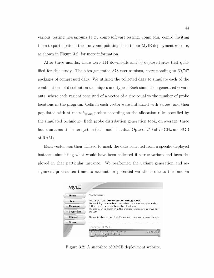
44
various testing newsgroups (e.g., comp.software.testing, comp.edu, comp) inviting
them to participate in the study and pointing them to our MyIE deployment website,
as shown in Figure 3.2, for more information.
After three months, there were 114 downloads and 36 deployed sites that qual-
ified for this study. The sites generated 378 user sessions, corresponding to 60,747
packages of compressed data. We utilized the collected data to simulate each of the
combinations of distribution techniques and types. Each simulation generated n vari-
ants, where each variant consisted of a vector of a size equal to the number of probe
locations in the program. Cells in each vector were initialized with zeroes, and then
populated with at most hbound probes according to the allocation rules specified by
the simulated technique. Each probe distribution generation took, on average, three
hours on a multi-cluster system (each node is a dual Opteron250 of 2.4GHz and 4GB
of RAM).
Each vector was then utilized to mask the data collected from a specific deployed
instance, simulating what would have been collected if a true variant had been de-
ployed in that particular instance. We performed the variant generation and as-
signment process ten times to account for potential variations due to the random
Figure 3.2: A snapshot of MyIE deployment website.

45
assignment of probes to variants, and from variants to instances. In this dissertation,
we assume that the number of variants n = 36, that is, we have as many variants as
deployed instances which constitutes an upper bound on the potential distribution.
3.3.2 Independent Variables
We manipulated the following variables. First, we defined four levels of overhead
bounds: 5%, 10%, 25%, and 50% over the non-instrumented program. To approxi-
mate the number of probes corresponding to the chosen levels of overhead, we inserted
a number of probes in random locations of the program associated with call-chains,
ran the available test suite, measured the overhead, and repeated the procedure while
adjusting the number of inserted probes until we converged on the target overhead
level. This resulted in four bound levels, hbound, as defined by the following number
of probes: 50, 75, 230, and 450.
We then implemented the three types of techniques illustrated in Section 3.1 by
varying the strategies and probe placement types:
• Probe-based distributions: Random-Probes (R Pr) and Balanced-Probes (B Pr).
• Property-based distributions: Random-Properties (R Pp), Balanced-Properties(B Pp),
Packed-Properties(P Pp) and Balanced-Packed-Properties(BP Pp).
• Cluster-based distributions: Random-Clusters (R Cl), Balanced-Clusters(B Cl),
Packed-Clusters (P Cl), and Balanced-Packed-Clusters(BP Cl).
While the Probe-based distribution techniques operate without prior information
about the properties to profile, the Property-based and the Cluster-based techniques
require some initial call-chain information. In this study, we denote the main method
of MyIE and all methods that represent event handlers as root methods of a call

46
graph. We denote a method as a leaf of a call graph if there exists no call from that
method to any other methods in the program. We do not consider loops or any back
edges in the graph and we exclude calls to external libraries.
To apply the Property-based distribution techniques, we needed to generate an
initial list of properties (call-chains). We generated this statically by analyzing a call-
graph of the application with the support of the Microsoft Studio C++ 6.0 navigation
tool-set. We hand-annotated the edges with the caller-site, adding extra edges when a
caller invoked a callee from multiple locations. We validated the graphs by examina-
tion and by running an available test suite to detect any other potential edges missed
by the static analysis tool. We then generated the list of call-chains in our object of
study by performing a depth-first search traversal of the graph2. This process yielded
12355 call-chains with a maximum size of 12 method calls and an average size of three
method calls.
To apply the Cluster-based techniques, we did not need to identify apriori the
set of properties to profile. Instead, we used a heuristic to define the clusters of
probes that may contain the properties of interest. We again utilized the call-graph
to identify our clusters, where each cluster included one root note and all the methods
reachable from that root. This yielded 556 clusters with a maximum size of 80 and
an average size of 11 method calls. To accommodate distribution techniques that can
satisfy hbound = 50, for clusters of the size > 50, we split them by treating their roots’
immediate children as the new roots and repeating the process until all clusters had
the maximum size of 50. We ended up with a total of 571 clusters.
For balancing and packing the Property-based and Cluster-based distributions,
we utilized Algorithm 3.2 with the parameters presented in Table 3.2. For any given
2Although we are aware of more precise techniques for generating call-chains (we discuss in Section3.3.4 why we did not pursue them and the impact of such a choice), it is important to recognize thatthis is an inherent limitation of this type of technique.

47
Table 3.2: Hill Climb Simulation ParametersTechnique α β γ FROZEN
Balanced 0.5 0 0.5 500,000Packed 0 0.5 0.5 500,000Balanced-Packed 0.4 0.2 0.4 500,000
distribution, we want to ensure that each property is profiled at least once. Because
of this, the parameter γ is always set to be > 0. Balanced distribution is generated by
employing the concept of BALANCE. For this distribution, we set β to 0 (indicating
that PACKING of properties is not important). Moreover, we treat BALANCE
and ALLUSED to be equally important, setting α and γ to be 0.5. The parameters
for the Packed distribution were set following the same intuition, where we set alpha,
instead of β, to 0. Defining the parameters for the Balanced-Packed technique was
less trivial. We experimented with several combinations of values and found that
the specific values for α, β, and γ listed in Table 3.2 yield a small set of interesting
distributions to explore.
3.3.3 Dependent Variables
The dependent variable is the captured field information value, for which we have
selected two metrics. The first metric is the percentage of call-chains covered in
the field when using a given probe allocation technique with respect to the call-chain
coverage obtained by a theoretical optimal allocation technique, Opt. Given an hbound
level and the data collected from the field, Opt represents what would have been the
ideal distribution of probes across variants. Since we captured a complete block trace
during the deployment of MyIE, we were able to enumerate the call-chains that were
observed for each variant, determine the probes that a variant would need to observe
these call-chains, and approximate the Opt distribution aposteriori. For each variant
that required a number of probes which exceeds a hbound, we performed two passes

48
to reduce the instrumentation probes until the hbound constraint was met. First,
we tried to remove the probes corresponding to call-chains that were observed in
multiple variants. Since we guaranteed that at least one call-chain can be observed
in one variant, no call-chain information is lost. If after this step we were still unable
to reduce the number of probes, we then removed the probes associated with the
shortest call-chain in a variant. This step may, however, cause us to lose some call-
chain observations.
The second metric aims to measure the false call-chains reported by each tech-
nique due to missing probes. A call-chain detected in the field is considered false
if (1) the call-chain is not detected by the Full technique (a technique that inserts
instrumentation in all units of the program), or (2) the call-chain is detected by the
Full technique, but it is not detected at the same location in the trace file as Full.
3.3.4 Threats to Validity
From an external validity perspective, our findings are limited by the artifact of
study, the data-collection process, and the user population. Although it is arguable
whether the selected program is representative of the population of all programs, there
are many similar browsers to MyIE, making it a credible experimental object. During
instrumentation and data collection we attempted to balance data representativeness
and power through the utilization of full data capture combined with simulation. The
deployment and download process, as perceived by the users, was identical to many
other sites offering software downloads and on-line patches. Further studies with
other programs and subjects may be necessary to confirm our findings.
From an internal validity perspective, the quality of the collected field data
is an important threat as packages of field data may get lost, corrupted, or not
sent. We controlled this threat by adding different stamps to the packages to en-

49
sure their authenticity and to detect any anomalies in the collection process. Ad-
ditionally, alternative definitions of call-site call-chains (e.g., fixed-length call-chains
or component-bounded call-chains) may influence the number of anomalies detected,
or the noise and the static analysis needed to generate the initial list of call-chains
for the Property-based technique may have limited their performance. Our choice
of call-chain definition was driven by practical considerations including limitations
in the static analysis tools which cannot fully process large C++ applications that
utilize MFC components.
The lossy mechanism which we have used to construct the Opt distribution is also
a potential threat to validity, where we repeatedly remove probes corresponding to
the shortest call-chain in order to satisfy the overhead constraint. Such construction
may potentially cause us to lose more call-chain observations than if we removed
probes corresponding to a longer call-chain. We measure the performance of each
technique with respect to Opt, and under-estimating the number of call-chains that
can be observed given an optimal distribution may cause an over-estimation of their
performance. However, longer call-chains may also contain probes that are used by
other observed call-chains in a variant, increasing the complexity of the mechanism.
Moreover, since we are only interested in understanding the performance of a tech-
nique relative to other techniques, and given that we measure each technique using
the same Opt distribution, our findings still hold.
From a construct validity perspective, we have chosen a set of metrics to quan-
tify the value of the collected information that captures only a part of its potential
meaning. Our choices are a function of our interest in exploiting field data for valida-
tion purposes, and our experience and available infrastructure to analyze such data.
Also, from a construct perspective, we have approximated the hbound and have chosen
a subset of the potential levels for it that attempt to operationalize a spectrum of

50
h_bound = 50 (5%)
0
10
20
30
40
50
60
70
80
90
100P
erce
ntag
e of
Cal
l-Cha
ins
Cor
rect
lyId
entif
ied
Mean ±SD Min-Max
h_bound = 75 (10%)
0
10
20
30
40
50
60
70
80
90
100
h_bound = 230 (25%)
R_PrB_Pr
R_PpB_Pp
P_PpBP_Pp
R_ClB_Cl
P_ClBP_Cl
Techniques
0
10
20
30
40
50
60
70
80
90
100
Per
cent
age
of C
all-C
hain
s C
orre
ctly
Iden
tifie
d
h_bound = 450 (50%)
R_PrB_Pr
R_PpB_Pp
P_PpBP_Pp
R_ClB_Cl
P_ClBP_Cl
Techniques
0
10
20
30
40
50
60
70
80
90
100
Figure 3.3: Identification of Call-Chains.
values that allow us to characterize the effects of the treatments.
From a conclusion validity perspective, we are making inferences based on a few
hundred sessions which may have limited the power to detect significant differences.
However, we were able to reject various hypotheses and discover interesting findings.
3.4 Results
We now compare the performance of probe distribution types (Probe-based, Property-
based, and Cluster-based) and techniques (random, balanced, and packed) across
different bound levels that restrict the number of probes placed in a given variant. We

51
start by performing an exploratory analysis of the data through the box plots in Figure
3.3, which depict the percentage of call-chains correctly identified by the deployed
instances (compared to what is achieved by the Opt technique) when utilizing the
distribution techniques for the chosen four levels of hbound (one per subfigure).
Property-based techniques (the techniques in the shaded area of Figure 3.3) and
Cluster-based techniques (the techniques to the right of the shaded area) perform
better than Probe-based techniques (the two left most boxes of each subfigure) in
terms of identifying correct call-chains for all bound levels. This suggests that sim-
ply allocating probes without associating them with the target properties is unlikely
to provide valuable data even in the presence of hbound values as high as 50%. We
also note that Property-based techniques perform at least as well as Cluster-based
techniques when hbound = 450, but consistently worse for lower hbound values. We con-
jecture that when hbound = 450, Property-based techniques can allocate larger sets
of probes, corresponding to longer call-chains, thereby increasing the chance to ob-
serve such call-chains. Additionally, in contrast to Cluster-based techniques that can
only allocate probes corresponding to multiple properties to one variant at a time,
Property-based techniques can spread the profiling of each property across different
variants. This, in turn, may increase the chance of observing the call-chains. We also
conjecture that the poor performance of Property-based techniques for lower hbound
might be caused by the imprecision in determining individual call-chains apriori. This
confirms that Property-based techniques can be beneficial when applied to properties
that can be easily enumerated, but in general a Cluster-based approach seems to be
better, independent of the hbound constraints. An engineer can take this into consid-
eration when deciding which techniques to use.
When comparing random techniques to the search-based techniques (balanced,
packed, and balanced packed) in terms of the correctly identified call-chains we found

52
Table 3.3: p-values of the ANOVA TestHypotheses Effect p-value
H1 Type(Probes, Properties, Clusters) 0.00H2 Techniques Probes 0.069
(R, B, P, BP) Properties 0.00Clusters 0.00
H3 hbound 0.00H4 Techniques & hbound Probes 0.51
(R, B, P, BP) Properties 0.363Clusters 0.00
that, within Property-based techniques, the improvement provided is negligible, and
within Cluster-based, balancing and packing may provide some benefits (7% over
random on average).
To formally determine whether the observed tendencies were the result of chance
and to evaluate our hypotheses, we performed an ANOVA on the dependent vari-
able (correctly identified call-chain) and the three independent variables (type of
distributions, techniques, and hbound). The analysis of techniques and hbound was per-
formed independently within each distribution type. The summary of the p-values
of the analysis is shown in Table 3.3. P-values smaller than 0.05 indicate a signifi-
cant relationship between the treatment and the dependent variable that cannot be
attributable to luck, and should be interpreted as a rejection of the null hypothesis.
The p-values in Table 3.3 show that the correct percentage of call-chains reported
by the deployed sites varies significantly across different types of distribution and
bounds (H1). The distribution techniques did not seem to matter when utilizing
Probe-based distributions, but they did within the Property-based and Cluster-based
distributions (H2). As expected and overall, the hbound level did affect the dependent
variable (H3), but it was interesting to see that its effect within the Cluster-based
distribution had a significant interaction (H4).
We further explored the interaction within the Cluster-based distribution through

53
Table 3.4: Homogenous groups of Cluster-based distributionTech hbound Mean of Homogeneous
Detection Value Group
Random 50 22.6 APacked 50 28.2 A BBalanced 50 28.6 A BRandom 75 29.6 B CBal-Packed 50 29.42 B CPacked 75 33.9 B C DBalanced 75 35.7 C DBal-Packed 75 36.5 DPacked 230 44.4 ERandom 230 57.2 FBalanced 230 62.5 F GBal-Packed 230 62.92 F GPacked 450 66.27 GRandom 450 74.6 HBal-Packed 450 74.7 HBalanced 450 75.8 H
a Bonferroni analysis. A Bonferroni analysis compares all pairwise combinations of
techniques and hbound to quantify when a technique really did have a significant effect
on the call-chain detection. The result of this analysis, as presented in Table 3.4,
consists of a list of all potential combinations of techniques and bounds, their mean
values, and a letter representing the group to which the combination belongs (i.e., two
combinations that are assigned different letters are significantly different). We found
that when hbound is 50 (5%) and 75 (10%) the balanced-packed techniques enabled the
detection of a significantly higher percentage of correctly identified call-chains than
random. When hbound is 230 (25%) and 450 (50%), we could not detect differences in
the performance of random, balanced, and balanced-packed techniques (their means
belong to the same group). This means that only under tight overhead bounds do
our techniques make a difference.
Figure 3.4 shows the ratio of falsely reported call-chains over the correctly iden-
tified ones across the three types of distributions. For each type of distribution, we

54
Probe-Based Techniques
R_Pr_50B_Pr_50
R_Pr_450B_Pr_450
0.0
0.1
0.2
0.3
0.4
0.5
0.6
0.7
0.8
0.9
1.0
Rat
io o
f the
Num
ber o
f Fal
se C
all-C
hain
s ov
erth
e C
orre
ct C
all-C
hain
s
Mean ±SD Min-Max
Property-Based Techniques
R_Pp_50B_Pp_50
P_Pp_50BP_Pp_50
R_Pp_450B_Pp_450
P_Pp_450BP_Pp_450
Techniques - Bounds
0.0
0.1
0.2
0.3
0.4
0.5
0.6
0.7
0.8
0.9
1.0
Rat
io o
f the
Num
ber o
f Fal
se C
all-C
hain
sov
er th
e C
orre
ct C
all-C
hain
s
Cluster-Based Techniques
R_Cl_50B_Cl_50
P_Cl_50BP_Cl_50
R_Cl_450B_Cl_450
P_Cl_450BP_Cl_450
Techniques - Bounds
0.0
0.1
0.2
0.3
0.4
0.5
0.6
0.7
0.8
0.9
1.0
Rat
io o
f the
Num
ber o
f Fal
se C
all-C
hain
sov
er th
e C
orre
ct C
all-C
hain
s
Figure 3.4: Falsely Reported Call-Chains.

55
show all techniques on two extreme bound values (50 and 450). We can see different
tendencies between Probe-based, Property-based, and Cluster-based types as hbound
increases: the number of falsely reported call-chains by the Probe-based techniques,
as shown by the top box-plots, increases while the number decreases for Property-
based and Cluster-based types (middle and bottom box-plots). We conjecture that
in the case of Probe-based techniques, the more probes that are inserted, the more
they may lead to partial, and hence ambiguous, property observations in a variant.
In contrast, in Property-based and Cluster-based types, increasing hbound increases
the likelihood that longer call-chains are accommodated, thereby reducing the num-
ber of falsely reported call-chains. The false call-chains reported by Cluster-based
techniques were also contributed from partial observations due to our chosen mecha-
nism in constructing the cluster (where we ensure that each cluster’s maximum size
is 50). We can, instead, remove the maximum size constraint but with a trade-off of
potentially detecting smaller number of call-chains for hbound = 50 and hbound = 75.
We observe, however, that Packing and Balanced Packing can reduce the number of
false reports by encouraging a distribution where multiple clusters that were formed
from splitting a cluster to be allocated to the same variant.
More interesting, however, when hbound is 50, Property-based types yielded higher
number of falsely reported call-chains than the Probe-based types. We note that
the Property-based distributions are prone to reporting false call-chains under tight
hbound because there are not enough probes to discriminate between the monitored
properties and those that subsume them. Furthermore, in addition to having a large
variance (0.055), the number of falsely reported call-chains in the Property-based
techniques is ten times higher than the Cluster-based technique when hbound is 50.
This value improves significantly when hbound is 450, though it is still eight times
higher than the number falsely reported by the Cluster-based technique. Recall that

56
when generating clusters of probes, we grouped related call-chains (based on their
roots) together, hence decreasing the chance of observing an incomplete call-chain
because of missing the necessary probes in a variant.
Implications. When the acceptable overhead that bounds the profiling effort is small
(less than 10% in our study), Cluster-based allocation techniques that balance the dis-
tribution across clusters of probes are the most effective in retaining the value of field
data. Additionally, Cluster-based techniques are valuable when enumerating the prop-
erties is not feasible and when performing a heuristic search is too cost-inefficient,
in which case the Cluster-Random technique can be used. When hbound is 450, the
Property-based distribution seems to perform well regardless of the technique. In gen-
eral, any distribution technique working with clusters reported significantly fewer false
call-chains than the Probe-based and Property-based distributions, which translates
into savings for the engineer investigating such chains.
3.5 Conclusions and Future Work
Profiling overhead limits what we can observe and learn from deployed software. To
address this limitation, we investigated ways to distribute probes across variants to
meet profiling overhead constraints while maximizing captured field information. We
have formalized the problem of distributing probes across variants, presented several
distribution techniques, and carefully assessed their performance.
From our findings we can draw several interesting observations. First, the choice
of probe distribution techniques is crucial when overhead bounds are set below 10%
(a reasonable practice when the objective is to remain below the threshold of user
noticeability). Second, distributions that balance probes across variants perform con-
sistently better than those that do not, independent of the overhead bounds and the

57
type of distribution. Last, Cluster-based distributions tend to be less expensive to
set up than Property-based, collect more correct information than Property-based or
Probe-based, and report the least false information.
For continuing this work, we want to address the various costs involved in large-
scale profiling efforts. For example, analyzing the target program to relate probes to
properties may be expensive. We have shown that approximations through clustering
can be effective in lowering those costs but we have not yet quantified this. The cost
of the search algorithm can be computationally expensive, especially in the presence
of many target properties and profiling locations. More flexible convergence criteria
and more efficient implementations of the algorithms are necessary to make this ap-
proach scalable. We must also weigh the additional costs introduced by deploying and
maintaining multiple program variants, against the benefit of having more variants
to lower the amount of instrumentation per deployed instance. Future studies should
examine the trade-off between variants and bounds, and more generally, the costs and
benefits of large-scale profiling efforts. Finally, we are interested in studying the im-
pact of using feedback to adjust the sampling of properties, which we start exploring
in Chapter 4.

58
Chapter 4
Lattice-based Sampling for
Profiling Path Properties0
Engineers are often interested in profiling a program for its conformance with user-
defined path properties (also referred to as temporal, sequencing, or typestate prop-
erties). Path properties, commonly expressed as Finite State Automata (FSA), con-
strain the orderings of program event (e.g., method call) occurrences as expected by
their programmers, usually to ensure that the program will behave correctly. For ex-
ample, a path property for objects of the type java.nio.channels.SocketChannel
may specify that a method call read() should always be preceded by a method call
connect(). When profiling path properties, instrumentation probes are inserted to
enable observation of the relevant method calls. Whenever such method calls are ob-
served, the state of the FSA is updated and checked on-the-fly to ensure that method
calls orderings have not been violated.
As mentioned in Section 2.1, existing sampling efforts have approached the chal-
lenge of reducing overhead when profiling path properties in deployed environments
0Some of the work in this chapter has been previously published in [28].

59
by performing sampling across the allocated objects to select smaller number of in-
stantiated objects to profile [5, 10]. The profiling overhead from leveraging these
sampling strategies, however, still depends on the number of method calls that may
be performed on the objects. Instead, we choose to sample over the method calls con-
strained by a path property. Such sampling approaches share similar challenges as
sampling approaches for profiling complex state properties: both aim to enable profil-
ing of properties requiring multiple probes. Because of this similarity, the search-based
sampling approach introduced in Chapter 3 can be utilized to allocate instrumenta-
tion probes for sound path property profiling (provided we can precisely enumerate or
over approximate program locations that are needed to profile the path properties).
We recognize, however, additional opportunities unique to path properties that
we leveraged to develop a sampling strategy specifically targeted for profiling them:
(1) related path properties can be used to compose a larger and a more complex prop-
erty that constrains more diverse paths of method calls, (2) this integrated property
can be systematically decomposed to generate properties constraining alphabets of
symbols (i.e., sets of method calls) with varied size and cost to observe them, (3)
the decomposed properties can be ordered according to the method calls that they
constrain, as a lattice of properties where a violation of a property implies violations
of all the properties that subsume it, and (4) the properties can be associated with
weights to more effectively guide the sampling process.
Additionally, when profiling path properties, we may be faced with the need to
change the allocated probes during a deployment to adjust the profiling activity. As
discussed in Section 2.1, such change may be triggered by what we have learned
from the field information or from mismatches between the profiled events and the
observed events. Ignoring the need to make this adjustment may cause a waste in
profiling effort, providing no field information (such as in the case of mismatch) or field

60
information that is less useful to the engineers. When adjusting the probe locations,
however, we have to be aware of the challenge of choosing the next relevant path
properties to profile, i.e., ones that can provide information of value to the engineers.
For example, if we have observed that a path property constraining the sequence
of methods A, B, and C was violated because of the incorrect orderings of methods
A and B, profiling a path property corresponding to methods A and B in the future
will not provide additional insights to the engineers when they are interested in only
exposing new violations, and the profiling and deployment efforts will be wasted. This
suggests the need for a technique to guide the sampling strategy in selecting future
path properties when the profiling activity is adjusted.
We address the challenges of profiling path properties more efficiently and effec-
tively, either due to profiling overhead or profiling adjustment, by (1) developing a
sampling technique that operates on a lattice of properties and their weights and (2)
proposing a mechanism to update the properties’ weights in the presence of profiling
feedback.
4.1 A Motivating Example
Consider the problem of profiling for correct usage of the java.nio.channels.Socket
Channel API. SocketChannels support networked IO in Java. The standard use-
case for an instance of a SocketChannel is to open and connect a channel, then
perform a series of read and write operations on the channel, and finally to close
the channel. There are, however, many other operations that can be performed on
SocketChannels, for example, open and connect can be performed in a single step
with a call to open(A) passing a socket address A.
Table 4.1 lists a collection of path properties extracted from the SocketChannel

61
(1) open() or open(A) beforeclose()
[close]* | ~[close]*;(open|openA);.*
(2) open() before connect() ~[connect]* | ~[connect]*;open;.*(3) close() after open() or
open(A)~[open,openA]*; ((open|openA);~[close]*; close; .*)?
(4) connect() or open(A) beforeread() or write()
~[read,write]* | ~[read,write]*;(connect|openA);.*
(5) no read() or write() afterclose()
~[close]*; (close; ~[read,write]*)?
(6) socket() beforeshutdownIn(Out)put()
~[shutIn,shutOut]* | ~[shutIn,shutOut]*;socket;.*
(7) no read() aftershutdownInput()
~[shutIn]*; (shutIn; ~[read]*)?
(8) no write() aftershutdownOutput()
~[shutOut]*; (shutOut; ~[write]*)?
Table 4.1: SocketChannel properties as specification patterns and regular expres-sions.
API documentation [81]. The English phrases, on the left, paraphrase text in the
class documentation using the terminology of the specification pattern system [27].
Regular expressions encoding these path properties are expressed in the Laser FSA
package’s syntax [48]. In this presentation, regular expressions are defined over names
of the public methods in the SocketChannel and Socket classes; in general, method
signatures would be used rather than the method names to treat overloading. In this
syntax, most operators, e.g., *, +, ., ?, have their standard meaning. In addition,
~[ ... ] denotes the complement of a symbol set, which is the disjunction of all
symbols not listed between the brackets, and ; denotes concatenation.
Consider an execution of an application that uses a single instance of SocketChannel
in the typical sequence 〈 open; connect; readk; writek; close 〉 where ak denotes k repe-
titions of a. The cost of profiling this application for the seven properties in Table 4.1
is (2k + 3)(co + 7cm) where co is the cost of executing the instrumentation to observe
a method call and cm is the cost of updating a property FSA. In Section 2.1, we have
mentioned several research efforts to reduce the number of (2k + 3) through static
analyses [9, 11, 30]. The cost of cm can be reduced by the use of clever data structures

62
and algorithms [9, 15]. Despite these advances, there still remain path properties for
real-world programs and APIs that cannot be effectively optimized and they can incur
overhead of greater than 150% [9].
Our Lattice-based Approach
One way to reduce profiling overhead is to integrate small properties into larger and
more comprehensive properties, and to profile the integrated properties instead. Ex-
pecting developers to write large complex path property specifications is problematic,
but they can be constructed through specification mining [2] or by directly composing
sets of smaller related properties [6, 10, ?]. We take the latter approach. Figure 4.1
is the product automata constructed from the FSA for all seven original properties
in Table 4.1; we denote this property as φ. This integrated path property is less ex-
pensive to profile than the seven properties independently since it will only require
(2k + 3)(co + cm) to profile, but it still detects the same violations as the original
properties. The real value of the integrated path property, however, lies in defining a
richer space of sub-languages that can be sampled to expose further cost-effectiveness
trade-offs in runtime profiling.
For example, Figure 4.2 illustrates FSAs defined over subsets of the original al-
phabet: {open, read} (on the bottom left) and {close, read} (on the bottom right).
These sub-alphabet properties were not in the original set of seven properties, but each
can be generated by projecting φ onto the sub-alphabet1. Profiling φ{close,read} for the
sequence of SocketChannel calls given above will cost (1 + k)(co + cm). Other sub-
alphabet properties, for example for {close, open, read}, shown on top of Figure 4.2,
encode a single property that enforces elements of multiple original properties, e.g.,
1Note that the automata in Figure 4.2 are limited by the original set of constraints extractedfrom informal API documentation. As such, they are incomplete and allow behavior that mightnormally be regarded as an error, e.g., open; open is accepted by φ{open,read}.

63
Figure 4.1: Integrated Constraint FSA–φ
properties (1), (3), and (5), yet avoids the cost of profiling all symbols in those prop-
erties, such as openA or write. Property φ{close,open,read} can be profiled at a cost of
(2 + k)(co + cm).
The penalty for reducing the profiling cost of sub-alphabet properties is a potential
loss of violation detection. For example φ{close,read} would miss violations where the
SocketChannel was not connected and φ{open,read} would miss violations where it was
not closed. Note, however, that any violation of these properties is guaranteed to be
a violation of the integrated path property φ.
Compared with the original seven properties, the space defined by φ includes 238
properties (including those illustrated in Figure 4.2) that are collectively capable of
the same violation detection as the original properties. Moreover, the sub-alphabet
properties of φ form a lattice that is ordered by the alphabet inclusion. Figure 4.3
shows a portion of the sub-lattice of φ that is rooted at φ{close,open,read,write} (the
symbols are referred to as c, o, r, and w respectively). The three FSAs in Figure
4.2 are part of this sub-lattice (they are shown shaded in Figure 4.3). Property

64
Ф{close, open, read}
Ф{open, read} Ф{close, read}
Figure 4.2: Sub-alphabet FSA
{c,o,r,w}
{c,o,w} {c,o,r} {o,r,w} {c,r,w}
{o,w} {c,o} {o,r} {c,w} {c,r}
{o} {c}
Figure 4.3: Property Lattice for φ{c,o,r,w}. The shaded properties are the three FSAsin Figure 4.3.
φ{close,open,read} subsumes φ{open,read} and φ{close,read} because its alphabet is a superset
of {open, read} and {close, read}. As we can observe from Figure 4.2, although
φ{open,read} and φ{close,read} are both subsumed by φ{close,open,read}, each property has
a distinct FSA structure. Note also that properties φ{read} and φ{write} are excluded
from the lattice even though their alphabets are subsets of {close, open, read, write}
because they are trivial properties, i.e., properties that unable to reject any streams
of method calls. Profiling trivial properties is not interesting because they cannot
detect any violation. The lattice of sub-alphabet properties is more diverse in terms

65
of profiling cost and violation detection ability than the original set of properties, yet
each sub-alphabet property is sound with respect to violation detection relative to
the original properties (i.e., if a sub-alphabet property reports a violation, it is also
violated by one of the original properties).
A sampling strategy can take into consideration the ordering in the lattice, for
example, to ensure that properties with differing violation detection are selected. Such
a strategy, when operating on the lattice of Figure 4.3, might first randomly choose
a property whose estimated profiling cost does not exceed a pre-defined overhead
requirement. Suppose that φ{c,o,r} is the selected property. Subsequently, the strategy
might attempt to choose a property whose alphabet includes some additional symbols.
For example, φ{c,w} might be chosen, but properties φ{c,o} or φ{o,r} would not be since
their alphabets are subsumed by {c, o, r}. Our approach might then deploy a program
variant that profiles φ{c,o,r} and φ{c,w} to a deployed site. Another program variant
that profiles a different set of path properties, following the same intuition, can be
deployed to another user site. This offers the potential to spread violation detection
across deployed sites.
Guiding the Sampling of Lattices of Properties.
When selecting which properties from the lattice to profile, it can be valuable to
guide the sampling strategy so that it favors the selection of certain properties. We
introduce a weighting scheme for a lattice to guide the sampling process where we en-
rich the lattice by assigning a weight to each its sub-alphabet properties. A sampling
strategy can then prioritize the selection of a property based on its weight. The initial
weights of the sub-alphabet properties can be defined, for example, by determining
potential infeasible method calls within a client application through its static analysis
(e.g., the weights of properties constraining unreachable method calls can be set to a

66
{c,o,r,w
{c,o,w} {c,o,r}* {o,r,w} {c,r,w}
{o,w} {c,o} {o,r} {c,w}* {c,r}
{o} {c}
highest
lowest
{c,o,r,w
{c,o,r,w
{c,o,w} {c,o,r} {o,r,w} {c,r,w}
{o,w} {c,o} {o,r} {c,w} {c,r}
{o} {c}
{c,o,w} {c,o,r} {o,r,w} {c,r,w}
{o,w} {c,o} {o,r} {c,w} {c,r}
{o} {c}
Figure 4.4: Weight Propagation for Lattice for φ{c,o,r,w} in the Case of Non-violatedProperty. The weights of the property is represented as shades of grey. Propertiesmarked by an * are profiled and properties marked by a check mark were actuallyobserved.
very low value), or by profiling executions to estimate their frequency of occurrence
and cost of observation.
Continuing with our previous example of Figure 4.3, Figure 4.4 illustrates three
weighting schemes for a lattice of φ{c,o,r,w}. For simplicity, we represent the properties’
weights by shading the lattice elements, where the darker the nodes are, the less
weight they have. Suppose that, initially, all the properties in the lattice start with
an equal weight, colored as white, as shown on the top of Figure 4.4. By incorporating
the weighting scheme, we can modify the previous sampling strategy to first select
properties with the highest weight value. Since all the properties initially have the
same weights, the sampling strategy will initially operate like the one in the previous

67
example and select φ{c,o,r} and φ{c,w} to be profiled (shown with an * in Figure 4.4).
Collected field observations can be then be used to adjust the properties’ weights.
Suppose that the feedback from a completed execution revealed that no calls to
read() were made during the execution, and φ{c,o} and φ{c,w}, instead of φ{c,o,r},
were observed (shown with a check mark in Figure 4.4). Moreover, the feedback also
revealed that these properties were not violated. Suppose also that we want to adjust
the properties’ weights such that the priority of the observed properties are lowered
(we defer discussion regarding this heuristic until Section 4.2.5).
We process the check marked properties one at a time, starting with φ{c,o} as
shown by the weighting scheme in the middle of Figure 4.4. Since φ{c,o} was ob-
served, we want to decrease the likelihood that this property will be profiled in the
future by decreasing its weight, hence the property is given a darker shade of gray.
Moreover, since φ{c,o} subsumes properties φ{c} and φ{o}, and observations on φ{c,o}
imply observations on φ{c} and φ{o}, their weights would be decreased as well. The
properties φ{c} and φ{o} are referred to as the sub-properties of φ{c,o}. On the other
hand, properties φ{c,o,w}, φ{c,o,r}, and φ{c,o,r,w} subsume the property φ{c,o}, and we
refer to them as the super-properties of φ{c,o}. Observing φ{c,o} means that we have
also observed some behavior of its super-properties; but, since only a portion of their
behavior was observed, their weights are decreased by a smaller amount than that
of the property φ{c,o}. Suppose that the weight is decremented proportional to the
number of shared alphabets between two properties. At this point, properties φ{c,o,w},
φ{c,o,r}, and φ{c,o,r,w} have a lighter shade of gray, showing that their weights are larger
than φ{c,o}’s. Moreover, property φ{c,o,w} is shaded lighter than φ{c,o,r} and φ{c,o,r,w}
since φ{c,o,w} shares fewer common symbols (method calls) to φ{c,o} than φ{c,o,r} and
φ{c,o,r,w} to φ{c,o}.
The bottom of Figure 4.4 shows the final weighting scheme after our approach has

68
{c,o,r,w}
{c,o,w} {o,r,w} {c,r,w}
{o,w} {c,o} {o,r} {c,w} {c,r}
{o} {c}
{c,o,r}* x
highest
lowest
Figure 4.5: Weight Propagation for Lattice for φ{c,o,r,w} in the Case of Violated Prop-erty
processed the feedback that φ{c,w} was observed but not violated. First, the weight
of φ{c,w} is reduced to reflect this observation; and now it has the same weight as
property φ{c,o}. Property φ{c} is the sub-property of φ{c,w}, and its weight is further
decreased (now has a darker shade of gray when compared to the middle graph in
Figure 4.4). The weights of its super-properties, φ{c,o,w}, φ{c,r,w} and φ{c,o,r,w}, are
also decreased. Using the current weighting scheme, since properties φ{o,r,w}, φ{o,r},
φ{o,w}, and φ{c,r} have the highest weights among the other properties in the lattice,
they are likely to be selected next by the sampling technique.
We can apply a similar heuristic in adjusting the properties’ weights when a vi-
olation in a property has occurred. Intuitively, when a property is observed to be
violated, then profiling this property provides less information with regard to the
correctness of the program. Figure 4.5 illustrates the weighting scheme of the lattice
after φ{c,o,r} was observed and violated (shown with * and x marks). The weight
of φ{c,o,r} is reduced to reflect a decrease in the interest of profiling this property.
Suppose that the weight of violated properties is decreased more than the ones of not
violated properties. This results in the color of the node associated with φ{c,o,r} being
changed to black. Similarly, the weight of its super-properties, φ{c,o,r,w}, should be
decreased by the same value since a violation to φ{c,o,r} implies that φ{c,o,r,w} was also
violated.

69
When adjusting the weights of the sub-properties of φ{c,o,r}, we need to evaluate
these properties individually to determine whether the violation of φ{c,o,r} means that
they were violated as well. This requires that the violating string is available as part
of the profiling feedback. Suppose that φ{c,o,r} was violated because read() occurred
before open(). Clearly the projection of the violating string onto the alphabet {o, r}
will violate φ{o,r}, but not φ{c,o}, φ{o}, or φ{c}. In this case, the weight of property
φ{o,r} is decreased and the node associated with φ{o,r} is given the color of black.
Meanwhile the nodes of φ{c,o} or φ{o} are given a darker shade of gray to show their
weight decrease that corresponds to the properties being observed but not violated.
4.2 Background, Definitions, and Approach
We now describe the foundational concepts for generating a space of properties that
can be sampled to profile path properties during program executions. Properties in
this space are automatically generated from a given set of target properties and (1)
represent necessary conditions for the target properties to hold, (2) offer a diversity in
cost and violation detection power, and (3) are related to each other via a refinement
relation. Then, we show how we enrich the property lattice with a weighting scheme
and how we adjust the weights through profiling feedback.
4.2.1 Profiling Path Properties
Path properties are commonly expressed in terms of observations of a program’s
behavior. An observation may be defined in terms of a change in the data state of
a program, the execution of a statement or class of statements, or some combination
of the two. For simplicity, we only consider observations that correspond to method
calls. We define an observable alphabet, Σ, as a set of symbols that encode observations

70
of program behavior.
For run-time profiling, the most common form of path property specification
used is a deterministic finite state automaton (FSA) [43]. An FSA is a tuple φ =
(S, Σ, δ, s0, A) where: S is a set of states, Σ is the alphabet of symbols, s0 ∈ S is
the initial state, A ⊆ S are the accepting states and δ : S × Σ → S is the state
transition function. We use ∆: S × Σ+ → S to define the composite state transi-
tion for a sequence of symbols from Σ. We define a trap state as strap ∈ S such that
¬∃σ ∈ Σ∗ : ∆(strap, σ) ∈ A. A property defines a language, or set, of words L(φ) = {σ
| σ ∈ Σ∗ ∧∆(s0, σ) ∈ A}.
FSA profiling involves instrumenting a program to detect each occurrence of an
observable, a ∈ Σ. The analysis stores the current state, sc ∈ S, which is initially
s0, and at each occurrence of an observable, it updates the state to sc = δ(sc, a) to
track the progress of the FSA in recognizing the sequence of symbols for the program
execution. The analysis detects a violation whenever sc = strap or when the program
terminates with sc 6∈ A. We say that a program execution, t, violates a property, φ,
if the sequence of observable symbols, σ, corresponding to t ends in a non-accepting
state, σ 6∈ L(φ).
Different approaches to checking program-property conformance produce qualita-
tively different results. We want analyses that are sound with respect to reporting
violations; such an analysis may fail to report a violation when it occurs, but it will
never report a violation when one does not occur. Moreover, we are interested in pro-
ducing such reports while reducing checking overhead. Our basic strategy involves
checking for violations of necessary conditions for φ; φ′ is a necessary condition for φ
if both are defined over the same alphabet and L(φ) ⊆ L(φ′).

71
4.2.2 Sub-alphabet Properties and the Lattice
To significantly reduce the cost of property profiling, one must reduce the number of
observable occurrences that are processed. One way to achieve this is to consider a
subset of the property’s observables.
Definition 4.2.1 (Sub-alphabet Property) Given an FSA, φ = (S, Σ, δ, s0, A), a
sub-alphabet property is φΣ′ = (S, Σ′, δ′, s0, A), where Σ′ ⊆ Σ and
∀a ∈ Σ′ : δ′(s, a) = δ(s, a)
∀a ∈ Σ− Σ′ : δ′(s, ε) = δ(s, a)
This definition yields sub-alphabet properties that are non-deterministic automata.
For convenience, we use φΣ′ to denote any equivalent automaton, e.g., a determinized
minimized FSA accepting the same language.
Since each sub-alphabet property of φ, φΣ′ where Σ′ ⊆ Σ, is defined over a dif-
ferent language than that of φ, we cannot simply consider language containment to
determine whether they constitute necessary conditions for φ. Instead, we require
that every word over Σ, whose projection onto Σ′ is rejected by φΣ′ , must also be
rejected by φ.
Proposition 4.2.1 (Necessary Sub-alphabet Properties) Let φ be an FSA, Σ′ ⊆
Σ, and πΣ′ : Σ∗ → Σ′∗ be the projection of words over Σ onto words over Σ′, then
∀σ ∈ Σ∗ : πΣ′(σ) 6∈ L(φΣ′) ⇒ σ 6∈ L(φ)
Note that Σ∗ simply refers to any sequence of symbols defined over alphabet Σ.
By Definition 4.2.1, φ and φΣ′ are isomorphic and every transition sequence in φ has a
corresponding sequence in φΣ′ where a ∈ Σ−Σ′ is replaced by ε. After a word σ, φΣ′
can be in a set of states ∆′(s0, π′Σ(σ)). Since φΣ′ is non-deterministic, ∆′(s0, π
′Σ(σ)) is

72
a superset of ∆(s0, σ) in φ. Consequently, (∆′(s0, πΣ′(σ)) ∩ A) = ∅ ⇒ ∆(s0, σ) 6∈ A.
Thus any sub-alphabet property is a necessary condition for the original property.
We denote the sub-alphabet property relation φΣ′ � φΣ, for alphabets Σ′ ⊆ Σ.
The three FSAs shown in Figure 4.2 are examples of necessary sub-alphabet prop-
erties of the integrated FSA of Figure 4.1. The bottom left of Figure 4.2, for instance,
is derived by taking the projection of the sub-alphabets {open, read}; while the bot-
tom right FSA is produced by projecting the sub-alphabets {close, read}. Hence,
φ{open,read}, φ{close,read} � φ{close,open,read}
4.2.3 The Lattice of Sub-alphabet Properties
Given an FSA φ, we define a lattice of sound properties for violation reporting relative
to φ by considering each of its sub-alphabet properties. The alphabet power-set
lattice, (P(Σ),⊆), induces a lattice of sub-alphabet properties.
Definition 4.2.2 (Lattice of Sub-alphabet Properties) Given a property φ, the
lattice of sub-alphabet properties, L φ consists of the set {φΣ′|Σ′ ⊆ Σ∧L(φΣ′) 6= Σ′∗}
ordered by �. > = φ, since ∀φ′ ∈ L φ : φ′ � φ. In general, there is a set of least
elements ⊥ = {φ⊥|¬∃φ′ ∈ L φ−{φ⊥} : φ′ � φ⊥}. Meet is defined as φΣ1 u φΣ2 =
φΣ1∪Σ2.
The term L(φΣ′) 6= Σ′∗ in Definition 4.2.2 means that ∃σ ∈ Σ′∗ : σ 6∈ L(φΣ′),
and explicitly excludes trivial properties that are incapable of rejecting a word from
the lattice L φ. Trivial properties lie toward the bottom of the lattice and the least
properties are the ones with the smallest alphabets that are capable of rejecting a
word. The sub-alphabet powerset and property lattices are isomorphic (except for
trivial properties), so we use the alphabet to denote the corresponding property. In
our presentation, we use Σ to denote the alphabet of the > property of a lattice L φ.

73
This lattice can be constructed using well-known algorithms on automata [43].
Since the lattice has at most 2|Σ| properties, it can be costly to construct for large al-
phabets. Determinizing non-deterministic automata may incur an exponential blowup
where given a non-deterministic automata with n states the resulting deterministic
automata can have up to 2n states. However, none of the path properties that we
have analyzed have the structure that leads to this blowup (the maximum state size of
the determinized automata we have seen is 81) and required little time to determinize
them.
Since sub-alphabet properties are constructed such that any trace that violates
a property, e.g., φ{close,read} (bottom right of Figure 4.2), is guaranteed to violate
properties with any superset of its alphabet, e.g., φ{close,open,read} (top of Figure 4.2);
a partial order on sub-alphabet properties, which can be used to define a lattice
of properties that is ordered by alphabet containment, can be induced. Intuitively,
this also gives rise to an ordering based on both violation detection effectiveness and
profiling overhead.
Property ordering in the lattice provides several sources of information that can be
exploited in sampling properties for profiling. For example, if the overhead of profiling
a property is too high, one might choose a property lower in the lattice, or if a property
detects no violations, one might choose a property higher in the lattice. In Section
4.2.5 we discuss our lattice sampling strategies which permit several optimizations to
control property sample construction cost and violation detection probability.
4.2.4 Weighting Scheme of a Property Lattice
Though orderings of the properties in a lattice can be leveraged by a sampling strategy
to select properties with varied (and complementary) violation detection capabilities,
static analysis and feedback from past executions provide other insights about the

74
properties (e.g., the likelihood of a property to be violated, the feasibility of observing
symbols that were constrained by a property) which should also be considered by the
sampling process to be effective. To introduce this complementary mechanism to
guide the selection strategy, one that does not directly relate to the ordering of the
lattice, we associate the lattice with a weighting scheme.
Definition 4.2.3 (Lattice Weighting Scheme) A weighting scheme of a lattice is
w: L φ → R.
Informally, a lattice weighting scheme is a function that maps each sub-alphabet
property φΣ′ of lattice L φ to a constant real value, which we refer to as a property’s
weight, w(φΣ′). In Section 4.2.5, we show a selection strategy that leverages the
weights of the sub-alphabet properties in the lattice.
Adjusting Lattice Weighting Schemes through Feedback. Various forms of
feedback from past executions and static analysis can be utilized to adjust the weights
of the sub-alphabet properties. Our strategy mainly relies on utilizing the feedback
about property observations and violations that were revealed from prior profiling
activities. To achieve this, additional information may need to be collected, e.g.,
alphabets’ coverage vector, alphabets’ counts, violating strings, or observed sequences
of symbols.
Different types of feedback offer different trade-offs between the cost of obtaining
it and the amount of information that can be inferred from it, which in turn may affect
the quality of weight adjustments. For example, one can simply collect a coverage
vector of the profiled properties’ symbols. Such information requires only a 1-bit
vector of the size of the alphabet; however, inferring the violating strings and the
number of times a property was observed in a run from such a vector is not possible.
On another extreme, one could collect the streams of symbols that were observed in

75
an execution. Such information is rich but its cost is proportional to the length of
the execution, which may become too expensive to collect.
Our approach assumes that information about property observations and viola-
tions can be obtained, regardless of whether they are estimated with the help of some
static analysis or exactly obtained from execution traces. Regardless of the specific
feedback that was collected and utilized to adjust a lattice weighting scheme, given
some observations about a property, we use the lattice structure to extend the ob-
servation of one property to other related properties in the lattice. We define two
property relationships. First, the super-properties of φ are those whose alphabets sub-
sume φ’s in L , super(φ) = {φ′ ∈ L : Σ′φ = Σ′
φ∪Σφ)}; this is equivalent to using t to
detect super-properties. Profiling super-properties of φ may be more expensive, but
allows capturing richer interactions between events. Second, the sub-properties of φ
are those whose alphabets are subsumed by φ’s, sub(φ) = {φ′ ∈ L : Σ′φ = Σ′
φ ∩Σφ)};
this is equivalent to using u to detect sub-properties. Profiling sub-properties of φ
may be cheaper and can provide a shorter path to violation, but is more limited in
exposing possible interactions between events that could lead to violations.
We adjust the properties’ weights based on the following intuitions. For any
observed property, the feedback may reveal whether it was violated. When a property
φ is observed and violated, profiling that property offers less additional information,
so resources should be shifted to profile other properties. On the other hand, when
a property φ is observed but not violated, our confidence that the program conforms
to φ increases, and profiling such properties may be considered less interesting. To
reflect the decrease in the interest in the profiling of a certain property, we decrease
the weight associated with the property. We use these intuitions to define our two
heuristics for modifying the weighting scheme. Note that there are other heuristics
that can be utilized to adjust the lattice weighting scheme. However, the general

76
idea is that, over time, as more feedback is obtained, more parts of the lattice can be
pruned out and the space of properties which the sampling strategy operates on will
be smaller; but has the most potential for providing additional profiling information.
Definitions 4.2.4 and 4.2.5 show the general approach in reducing the weight of
the observed properties, non-violated and violated respectively, and in reducing the
weights of their related properties. The function red(...) in both definitions is used
to tune the amount of weight reduction. The function is first parameterized by the
observed property, φ. To differentiate the amount of reduction depending on whether
or not property φ is violated, it is also parameterized with a binary value, where the
value of 0 triggers the reduction function for a non-violated property and the value
of 1 triggers the reduction function for a violated property.
In the case when non-violated property, φnv, was observed, its weight is reduced by
red(φnv, 0, ...) (as defined in Def. 4.2.4). Similarly, the weights of the sub-properties
of the observed property, sub(φnv), are reduced by the same amount since all the
behavior in the sub(φnv) is also observed by φnv in accordance with the subsuming
relation of L . Adjusting the weights of super(φnv) is more subtle. Confirming the
correctness of φ means that at least some parts of φ′ ∈ super(φ) are also correct,
decreasing their likelihood to reveal a violation. We conjecture that this decrease
should occur at a rate proportional to what φ and φ′ have in common, as measured by
the function common(φ, φ′). Different definitions of common(φ, φ′) are possible. This
function can be instantiated, for example, to calculate the ratio between the shared
alphabet symbols or the common trap strings to the number of distinct symbols or
common trap strings, respectively, of φnv and φ′.
Definition 4.2.4 (Modification for NonViolated Observations) Given w(L ),

77
φ ∈ L , where φ is determined to be observed but not violated.
ModifyWeightNonViolated(w(L ), φ) = ∀φ′ ∈ L ,∀φ′ ∈ Lw(φ′)− = red(φ, 0, ...) if φ′ = φ ∨ φ′ ∈ sub(φ)
w(φ′)− = (common(φ, φ′) ∗ red(φ, 0, ...) if φ′ ∈ super(φ)
As defined by Def. 4.2.5, when a violated property φv was observed, its weight
is reduced by red(φv, 1, ...). The weight of each of the super(φv) are reduced by the
same amount because a violation in φv also means a violation in super(φv) occurred
due to the lattice ordering. Each of the sub(φv), on the other hand, may or may not
be violated, as we have illustrated in Section 4.1. We differentiate the operation of
weight reduction for sub(φv) into two. If φ′ ∈ sub(φv) is also violated, its weight is
reduced by the same amount as φv, red(φv, 1, ...). Meanwhile, if φ′ ∈ sub(φv) is not
violated, its weight is reduced by red(φnv, 0, ...), signifying that φ′ is observed, but
not violated.
Definition 4.2.5 (Modification forViolated Observations) Given w(L ), φ ∈
L , where φ is determined to be observed and violated.
ModifyWeightViolated(w(L ), φ) = ∀φ′ ∈ L ,
=
w(φ′)− = red(φ, 1, ...) if φ′ = φ ∨ φ′ ∈ super(φ) ∨
(φ′ ∈ sub(φ) ∧ πΣ′(σ) 6∈ L(φ′))
w(φ′)− = red(φ, 0, ...) if φ′ ∈ sub(φ) ∧ πΣ′(σ) ∈ L(φ′)
The function red(...) can also be parameterized with additional information spe-
cific to the type of feedback that is collected. For example, one can reduce the weights

78
proportional to the number of times the property was observed:
red(φ, 0, numObserv(φ)) = numObserv(φ) ∗ c
where c is a constant value. If only a coverage vector is obtained, then numObserv(φ)
can be set to 1. Another criteria that can be used to tune the reduction amount is
by how thorough a property has been observed or violated. A property can accept
and reject a set of sequences of strings of symbols, and one can enumerate all acyclic
symbol sequences that lead to an accept and/or a trap state. Then, we can instantiate:
red(φ, ., numObserv(φ), numNewString(φ, σ)) =
numObserv(φ) ∗ c ∗ numNewString(φ, σ)
numString(φ)
where numNewString(φ, σ) counts the number of words that are uncovered by a
profiling execution and numString(φ) is the total number of the previously enumer-
ated words. The granularity of this enumeration can also be made finer by taking
into consideration the object in which the calls were performed.
4.2.5 Sampling of Property Lattice
Profiling cost can be reduced through sampling. Following the general sampling
problem as defined in Section 3.2, given φ to profile, we define Prop to be L φ and
CL ∈ Cluster as a set of instrumentation points to profile method calls or symbols
of each φΣ′ ∈ L φ. Our sampling approaches to profile path properties construct a
set of properties to be profiled by iteratively adding one property at a time into this
set. The techniques leverage the cost estimation for profiling each property to ensure
that each addition will satisfy the overhead budget, and several selection functions
that exploit the structure of the lattice, the structure of individual properties, and
the weighting scheme to predict the value of each addition to the set’s potential for

79
detecting violations.
Selecting Properties
Recall that any violation detected by a property implies that any property that sub-
sumes it will be able to detect that same violation. In other words, violations detected
by a subsuming property always contain the violation detected by the subsumed prop-
erties. The subsumption property inherent in the lattice can be exploited to restrict
sampling to properties with potential added value in terms of violation detection
relative to a given property set.
Definition 4.2.6 (Added Violation-detection) Given a set of properties P ⊆
L ,
addV d(P, L ) = {φ′|φ′ ∈ L ∧¬∃φ′′ ∈ P : φ′ � φ′′}
This definition defines the set of properties in lattice L that are not subsumed
by properties in P and thus have the potential to detect additional violations. In
our lattice example, as shown in Figure 4.3, if φ{c,o} ∈ P , then addV d(P, L ) = L -
{φ{c,o},φ{c},φ{o} }.
When sampling a space, one often wishes to achieve a measure of diversity in the
sampled set. One notion of diversity for properties in L φ measures the magnitude
of differences in property alphabet sizes. Intuitively, we conjecture that the more
alphabets that are “covered” by the selected properties, the more violations that we
can potentially detect. We define the alphabet difference between a sub-alphabet
property φΣ′ and a set of symbols α ⊆ Σ as alphaDiff(φΣ′ , α) = |Σ′ − α|.

80
Definition 4.2.7 (Max Alphabet Difference) Given P ⊆ L and alphabet α ⊆ Σ
maxAlpha(P, α) = {φΣ′ | φΣ′ ∈ P∧
¬∃φΣ′′ ∈ P : alphaDiff(φΣ′ , α) < alphaDiff(φΣ′′ , α)}
This defines the subset of path properties that are the most different in terms of
the number of unshared symbols with alphabet α. Continuing with our example,
maxAlpha(P, α) where α = {c, o} yields {φ{c,o,r,w}, φ{o,r,w}, φ{c,r,w} }.
Another notion of diversity can be defined in terms of the rejected symbol se-
quences for a given property by enumerating the set of strings that drive acyclic
transition sequences leading from the property’s start state to its trap state.
Definition 4.2.8 (Acyclic Trap Strings) Given φΣ,
traps(φΣ) = {σ | σ ∈ Σ∗ ∧∆(s0, σ) = strap∧
¬∃i 6= j : ∆(s0, σ[i]) = ∆(s0, σ[j])
where σ[i] denotes the prefix of σ of length i.
Trap strings can be used to order a set of properties in terms of the number of
new trap strings that a given property would add relative to a given set of properties.
In our example, traps(φ{c,o}) = { 〈open〉, 〈close〉, 〈close, open〉 }. Suppose that φ{c,o}
has been selected to be profiled and we are given the choice between profiling φ{o,r}
or φ{c,r} along with φ{c,o}. The previous diversity notion, i.e., the number of unshared
alphabets, will not able to differentiate between the two properties. However, with
respect to trap strings diversity relative to φ{c,o}, φ{c,r} will be selected instead of φ{o,r}
because |traps(φ{c,r}) - traps(φ{c,o})| = | { 〈read〉 , 〈close, read〉, 〈close, read, close〉
} | = 3, while | traps(φ{o,r}) - traps(φ{c,o}) | = | { 〈read〉, 〈read, open〉 } | = 2.

81
Definition 4.2.9 (Max Trap Strings) Given P, M ⊆ L ,
maxTrap(P, M) = {φ | φ ∈ P∧
¬∃φ′ ∈ P : |traps(φ)−⋃
φm ∈ M : traps(φm)| <
|traps(φ′)−⋃
φm ∈ M : traps(φm)|}
As shown through an example in Section 4.1, one can also define a selection
strategy that leverages weight annotations to bias the selection of a set of properties
with maximum weight.
Definition 4.2.10 (Max Weight) Given a set of properties P in the lattice, P ⊆
L ,
maxWeight(P ) = {φ′|φ′ ∈ L ∧
¬∃φ′′ ∈ P : w(φ′) < w(φ′′)}
Given a cost estimate for profiling a program relative to a set of observed program
events, cost : P(Σ) → Z, calculated, for example, by profiling a small set of runs, one
can select properties based on a given cost threshold.
Definition 4.2.11 (Cost Threshold) Given P ⊆ L , and a cost threshold value
hbound ∈ Z,
costThresh(P, hbound) = {φΣ′|φΣ′ ∈ L ∧cost(Σ′) < hbound}

82
Sampling Strategies
Figure 4.1 shows the core of our cost-aware property sampling strategy. In general,
given a threshold on profiling cost (hbound), our sampling strategy operates as follows:
while the threshold has not been reached, select the “best” remaining property from S,
update the set of properties (M) and the remaining cost threshold (hbound), filter the
remaining candidate properties by removing the ones that are subsumed by profiled
properties (addV d(M, L )) or are too costly, and continue.
Algorithm 4.1 General Property Sampling StrategyPROPERTY SAMPLE(L , hbound){cost = 0M = ∅S = costThresh(L , hbound)while (cost < hbound ∧ S 6= ∅) do
φΣ′ = select(S, . . .)M = M ∪ {φΣ′}cost = cost + cost(Σ′)S = costThresh(addV d(M,L ), hbound − cost)return M
}
Selection of properties can be performed in many ways; we explore several ap-
proaches based on the selection functions that are previously defined. Randomly
selecting a property from a given set, select(S, . . .) = rand(S), yields the basic sam-
pling strategy. Choosing properties with maximal alphabet diversity, select(S, . . .) =
rand(maxAlpha(S,⋃
φΣ ∈ M : Σ)), yields the symbol sampling strategy. Choosing
properties with maximal trap string diversity, select(S, . . .) = rand(maxTrap(S, M)),
yields the path sampling strategy. Composition of selection functions can also be used.
For example, select(S, . . .) = rand(maxAlpha(maxWeight(S),⋃
φΣ ∈ M : Σ))),
yields the weight-symbol sampling strategy that first favors selecting a property with
maximal weight value before selecting a property with maximal symbol coverage in
the case of ties.

83
4.3 Path Property Profiling Infrastructure Sup-
port
select(…)
Chosen-set of sub-properties
Chosen-set of sub-properties
Lattice Builder
Lattice Property Sampler
Chosen set of sub-properties (Фi)
Variant Generator
p p(Фi)
Monitoring Feedback
Weight Annotator
p(Фj)
.
.
.
EC1
Request id
EC2
Lattice Weighting
Scheme
Constraints
Coverage vector
Local Global
hbound
red(…)
Figure 4.6: Path Property Profiling Infrastructure
Figure 4.6 shows the infrastructure we have built to empirically investigate our
path property profiling approach. The squares in Figure 4.6 represent the compo-
nents of the infrastructure and the circles represent the outputs of the components.
The shaded area of the figure illustrates one of many possible deployment scenarios,
where each program variant will be deployed to one user site (we discuss several other
possible deployment scenarios in Section 4.4.1). To enable the exploration of the dif-
ferent deployment scenarios in our study, we have chosen to simulate the generation of
program variants and their deployments2. In the following section, we briefly describe
the infrastructure to provide their expected output, but we defer the discussion of the
actual implementation until Section 4.4.2. In the subsequent sections, we describe
the remaining components in greater detail.
2Our choice to perform simulation instead of real deployment is driven by the cost and timeconstraint for setting up and conducting the study.
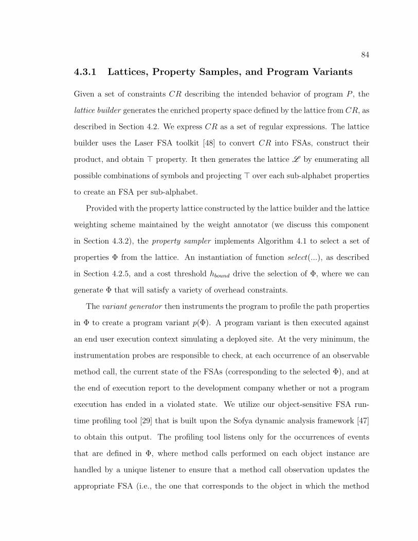
84
4.3.1 Lattices, Property Samples, and Program Variants
Given a set of constraints CR describing the intended behavior of program P , the
lattice builder generates the enriched property space defined by the lattice from CR, as
described in Section 4.2. We express CR as a set of regular expressions. The lattice
builder uses the Laser FSA toolkit [48] to convert CR into FSAs, construct their
product, and obtain > property. It then generates the lattice L by enumerating all
possible combinations of symbols and projecting > over each sub-alphabet properties
to create an FSA per sub-alphabet.
Provided with the property lattice constructed by the lattice builder and the lattice
weighting scheme maintained by the weight annotator (we discuss this component
in Section 4.3.2), the property sampler implements Algorithm 4.1 to select a set of
properties Φ from the lattice. An instantiation of function select(...), as described
in Section 4.2.5, and a cost threshold hbound drive the selection of Φ, where we can
generate Φ that will satisfy a variety of overhead constraints.
The variant generator then instruments the program to profile the path properties
in Φ to create a program variant p(Φ). A program variant is then executed against
an end user execution context simulating a deployed site. At the very minimum, the
instrumentation probes are responsible to check, at each occurrence of an observable
method call, the current state of the FSAs (corresponding to the selected Φ), and at
the end of execution report to the development company whether or not a program
execution has ended in a violated state. We utilize our object-sensitive FSA run-
time profiling tool [29] that is built upon the Sofya dynamic analysis framework [47]
to obtain this output. The profiling tool listens only for the occurrences of events
that are defined in Φ, where method calls performed on each object instance are
handled by a unique listener to ensure that a method call observation updates the
appropriate FSA (i.e., the one that corresponds to the object in which the method

85
call was performed).
Optionally, the program variant can also provide additional feedback that includes
(1) the acyclic transition sequence during profiling and (2) the set of symbols in the
alphabets that have been executed (symbol coverage vector). We note that recording
complete violating strings is cost-prohibitive, consequently we record, during profil-
ing, a transition sequence through the automaton that is acyclic. This sequence can
be only as long as the number of states in the automaton. Updating the sequence
can be performed very efficiently by maintaining a table for each pair of states corre-
sponding to a transition and performing a lookup on the table for every new transition
received. The string of transitions can also determine how complex path properties
may be violated, where violations are distinct if they trace different acyclic transi-
tion sequences through the property automaton to their final non-accept state For
example, the lack of a close or the presence of a write after a close represent two
distinct violations of φ{c,o,r,w} of Figure 4.2.
4.3.2 Weighting Scheme
The weight annotator is responsible for creating and updating a lattice weighting
scheme by annotating each sub-alphabet property with a weight value and adjusting
them as feedback is gathered. It starts by initializing the weighting scheme. The
default weights for all the sub-alphabet properties are 0.
As indicated in Figure 4.6, the weight annotator is parameterized by three pos-
sible inputs: the lattice to be associated with the weighting scheme, L , feedback
(in the form of observed or violated φ), and a request id (along with the symbols
coverage associated with user site id). The last two parameters are optional and,
when provided, regulate the scope in which feedback may impact the calculations of
the weight annotator.

86
We differentiate two feedback scopes: global and local. In global, feedback will
guide the selection of subsequent property selection. This is achieved by establishing
one global weighting scheme, in which any prior information will be used to adjust
the properties’ weights. When feedback about an observed property is provided, the
weight annotator will recalculate the weighting scheme employing the functions in
Def. 4.2.4 and Def. 4.2.5. In this dissertation, we instantiated red(...) functions
as follows: red(φ, 0) = 1 and red(φ, 1) = ∞, indicating our emphasis in pruning
properties that have been violated.
We conjectured that there is a potential for improvement by considering a sepa-
rate and localized weighting scheme for each execution context where the properties’
weights are adjusted based on the user site’s specific feedback. This localized feedback
is useful to further guide the sampling selection to reflect the characteristics of its par-
ticular execution context by pruning properties that have less chance of being observed
based on its execution history. For example, when a program variant is deployed at a
site that does not utilize certain symbols, the local feedback may then further reduce
the chance of properties related to these observables from being sampled in the future.
We use a coverage vector to record the set of symbols encountered on the program
execution associated with an execution context id. This is relatively inexpensive to
capture and its size is proportional to the size of the lattice alphabets. Coverage
vector allows the calculation of the observable properties for a run to estimate the
unobservable properties for a deployment site id, Φunobs(id) = {φΣ′ : Σ′ ∩Σobs(id) = ∅},
where Σobs(id) is the set of symbols present in the coverage vector.
When a request id is supplied to the weight annotator, the localized strategy is ini-
tiated and the property sampler will be performed on the localized weighting scheme.
The weight annotator will first check whether there exists a coverage vector associ-
ated with such an id in the profiling feedback database. If such a coverage vector

87
exists, then the global weighting scheme is copied to create a local weighting scheme.
Then, the localized weighting scheme is modified by pruning each Φunobs(id) from L ,
which is done by reducing their weights by ∞. If no coverage vector is found, the
weight annotator terminates. Since we always perform the local weight adjustment
on a copy of the global weighting scheme, the exclusion of Φunobs(id) only affects the
current sampling strategy. For future program variant generations, when a different
execution history gives rise to Φ′unobs(id) 6= Φunobs(id), then the newly observable prop-
erties, though previously unobservable, will not be pruned in L and will be available
for sampling to profile a deployed site id.
4.4 Empirical Study
In this section, we assess the performance of our approach through the following
research questions:
• How rich is the space of properties defined by the lattice (RQ1)? We would like
to explore the degree to which the lattice enriches a space of original properties
for a sampling strategy to operate on, specifically with respect to how property
violation detection varies with alphabet size.
• How effective are the various sampling strategies in detecting violations while
operating under a variety of overhead constraints? We would like to understand
their effectiveness under the different dimensions that define a deployment sce-
nario: the number of program variants generated (RQ2), the number of de-
ployments (RQ3), and whether or not resampling is performed and feedback
is used (RQ4).
In the next sections, we describe the deployment scenarios we are evaluating, the
study setup, the dependent and independent variables, and the threats of validity of

88
the study.
4.4.1 Deployment Scenarios
To answer our research questions, we require a deployment scenario for exploring
RQ2, RQ3, and RQ4. There are at least two dimensions that we can consider when
defining a deployment scenario: (1) the number of program variants generated and,
(2) the number of deployed sites (we refer to them simply as deployments). Each
program variant P (Φ) is responsible for profiling a set of properties Φ that is selected
according to some sampling strategy. Then, each program variant is deployed to
one or multiple execution contexts EC. Figure 4.7 shows five possible deployment
scenarios defined by these two dimensions.
Figures 4.7-a and 4.7-b illustrate the deployment scenarios where only one program
variant is generated. In these scenarios, only the sub-alphabet properties contained
in Φi can be potentially observed by P (Φi). In Figure 4.7-a, this program variant
is deployed to only one deployed site (EC1). Figure 4.7-b shows a program variant
deployed to multiple sites, where it may be exposed to a richer set of execution
behaviors. In RQ2, we investigate the performance of several sampling strategies
when we vary the number of deployments while fixing the number of variants; that
is, we evaluate the approach’s performances while moving from the strategy in Figure
4.7-a to the one in Figure 4.7-b.
Figure 4.7-c, 4.7-d, and 4.7-e depict deployment scenarios with multiple program
variants and multiple deployments. In Figure 4.7-c, each program variant is deployed
to a distinct execution context. We conjecture that with multiple program variants
across deployments, we may profile more path properties than if we employ only one
program variant. In RQ3, we compare the performance of the sampling strategies
across different number of variants and a fixed number of deployments. We are

89
c)
d)
e)
b)
a)
Variant Deployment
Фi P(Фi) EC1
Фi
P(Фi) EC1
P(Фi) EC2
P(Фi) EC3
P(Фi) EC1
P(Фj) EC2
P(Фk) EC3
Фi Фj Фk
P(Фi) EC1
P(Фj) EC2
P(Фk) EC3
Фi Фj Фk
P(Фi’) EC1
P(Фj’) EC2
P(Фk’) EC3
Фi Фj Фk’
P(Фi) EC1
P(Фj) EC2
P(Фk) EC3
Фi Фj Фk
P(Фi’) EC1
P(Фj’) EC2
P(Фk’) EC3
Фi Фj Фk’
Comparison
Single vs. Multiple Deployments
(RQ2)
Single vs. Multiple Variants (RQ3)
No-resampling vs. Resampling
Resampling Without Feedback vs. With Feedback
(RQ4)
Figure 4.7: Deployment Scenarios

90
interested in understanding the impact of different sampling strategies in selecting
sets of properties to be profiled across multiple program variants.
As the profiling activity is progressing, at certain points, new program variants
can be generated in an attempt to refine the profiling process. For example, after data
is received from a deployed site, a different program variant that profiles a new set of
properties may be generated and redeployed (mimicking the patching and feedback
processes that are commonly in place to support applications as they evolve). Figure
4.7-d and 4.7-e show such deployment scenarios with multiple variants generated
across time (in addition to across deployments). In these scenarios, we show two
ways for resampling properties for new variants.
In Figure 4.7-d, new variants are generated by randomly re-sampling the proper-
ties to profile. This scenario reflects a sampling strategy where a new set of properties
are profiled at predefined intervals. For example, consider a sampling over time (tem-
poral) strategy, where each set of instrumentation probes to profile a property might
be associated with a fixed sampling rate. After every fixed number of executions,
the sampling strategy selects, based on the sampling rate, which instances of the
probes would be invoked. In this scenario, different properties may be executed at
fixed intervals, “generating” a new program variant that profiles different sets of path
properties. The selection of the new set of properties is random and is generally
independent of the previous profiling cycle. In Figure 4.7-e, we consider an adap-
tive profiling scenario where re-sampling of the properties leverages information from
previously profiled data. We show a sampling strategy that uses a weighting scheme
that is continuously updated based on property observations and violations to drive
the sampling process.
For RQ4, we compare the profiling scenarios of multiple variants across deploy-
ments (Figure 4.7-c) with multiple variants across time and deployments (Figure

91
4.7-d and 4.7-e) to gauge the benefit of continually refining the selection of profiled
properties. Moreover, we want to evaluate the performance of techniques that lever-
age feedback (strategy in Figure 4.7-e) when compared to ones that do not leverage
feedback (Figure 4.7-d).
4.4.2 Study Setup
To answer the research questions we required a representative artifact with a set of
path properties that we could profile, clients that may use the artifact in ways that
violate its defined properties, and a simulation environment for each of the profiling
scenarios. We outline our study setup in Figure 4.8.
APIФn
…
Simulates deployment
Site1
Siten
Site1
Siten
.
.
.
.
.
.
…
API Т
CP1
CP2
CP3
CP4
Mutates program
Executes program
t1(M1)m1_1 m1_1 m1_1 M1
m1_1 m1_1 m1_1 M2
m1_1 m1_1 m1_1 M3
m1_1 m1_1 m1_1 M4
Simulates sites
Test Suite
T
…
…
…
…
4 5
Lattice of sub-alphabet
properties APIФ1
φorig_2
φorig_1
φorig_i
Builds lattice
Samples properties
Generates variants
API
.
.
. 1 2
3
7
6
Т
φlat_1
φlat_2
.
.
.
φlat_j
φlat_u φlat_v
to(M1)
t1(M2)
t1(M3)
t1(M4)
tp(M2)
tq(M3)
tr(M4)
tk(M1) tl(M1)
…ts(M4) tt(M4)
Ф1
Фn
Figure 4.8: Overview of Study Setup for Path Property Profiling
Artifact. We selected Hibernate, an open source Java library that provides support
for object persistence [41], as our artifact. Its core library, Hibernate Core 3.2, consists
of 78 Java KLoC, is downloaded thousands of times a day, and is used by hundreds

92
(1) sf.openSession() orsf.getCurrentSession()before anything
(openSession|getCurrentSession);.*
(2) sf.openSession() befores.close()
~[close]* | ~[close]*;openSession;.*
(3) s.close() or s.disconnect()after sf.openSession()
~[openSession]*;(openSession;~[close,disconnect]*; (close|disconnect);.*)?
(4) s.close() or s.disconnect()or tx.commit() aftersf.getCurrentSession()
~[getCurrentSession]*; (getCurrentSession;~[close,disconnect,commit]*;(close|disconnect|commit);.*)?
(5) s.beginTransaction() beforetx.commit()
~[commit]* | ~[commit]*;beginTransaction;.*
(6) tx.commit() afters.beginTransaction
~[beginTransaction]*;(beginTransaction;~[commit]*;commit;.*)?
(7) tx.beginTransaction() ortx.getTransaction before anyobject related operations (e.g.,s.get(A))
~[refresh,save,saveOrUpdate,get,delete,lock,load,clear,update]*|~[refresh,save,saveOrUpdate,get,delete,lock,load,clear,update]*;(beginTransaction|getTransaction);.*
(8) s.load(A) or s.get(A) be-fore any object changing op-erations (e.g., s.update(A) ors.delete(A))
~[save,saveOrUpdate,delete,lock,update,refresh]* |~[save,saveOrUpdate,delete,lock,update,refresh]*;(get|load);.*
(9) No object changing opera-tions (e.g., s.update(A)) afters.delete(A) unless precededby s.get(A) or s.load(A)
~[delete]*; (delete; ~[refresh,get,load,save,lock,saveOrUpdate,update]*;(get|load);.*)?
Table 4.2: Hibernate properties as specification patterns and regular expressions.
of other open source projects (including the Apache web server).
We derived path properties for Hibernate following the guidelines described by
Dwyer et al., [27]. We examined the Hibernate API and its documentation, identi-
fied recommended usage patterns (and anti-patterns) that could be translated into
constraints, and then translated those constraints into properties represented by reg-
ular expressions. We focused on the usage of transactions and object processing API
calls while considering the three possible states of objects in Hibernate (transient,
persistent, and detached) [8, 41]. The resulting property set has nine path properties
that include 17 Hibernate API calls appearing in the Session, SessionFactory, and
Transaction classes. Given SessionFactory sf, Session s, and Transaction tx.
These properties are shown in Table 4.2.

93
We encoded Hibernate’s nine original path properties as regular expressions (as
in Table 4.1). Note that this set of original path properties corresponds to CR in
our infrastructure (as shown in Figure 4.6). We feed CR to the lattice builder of
our infrastructure to generate >. The resulting > has 81 states, where 21 of the
states are accepting states. The tools enumerate all possible combinations of symbols
(API calls), resulting in the generation of 131,071 sub-alphabets, and project > over
set of each sub-alphabet properties to create an FSA per sub-alphabet. Finally, the
trivial FSAs are discarded resulting in an L φ with 106,340 non-trivial sub-alphabet
properties. These processes correspond to steps one and two (shown as diamond
boxes) in Figure 4.8. The process to generate the lattice took approximately two
days on a multi-cluster system (each node is a dual Opteron250 of 2.4GHz and 4GB
or RAM). Although this cost is not trivial, we could, however, lower it by employing
on-demand construction of sampled properties. We discuss the alternative mechanism
for constructing the lattice in Section 4.4.4.
Clients. We illustrate the process for preparing the client applications in step 3 of
Figure 4.8. First, we selected four open source applications as clients (p1 to p4 in
Figure 4.8) that utilize Hibernate: 1) an online auction application (AS) that comes
with the Hibernate package to illustrate its usage [8], 2) a WebStore (WS) online
shopping application [85], 3) NoteCat (NC) a web based application to manage Wiki
notes [67], and 4) iTracker (TR) a project planning and issue tracking application
[84]. The average client size is 4K LOC. To drive the execution of the clients, we
use an enhanced version of their test suites. We added tests to the original suites to
exercise the clients more extensively so that, in turn, they would execute their calls
to the Hibernate API, allowing us to check for path property violations.
To simulate usage violations of the Hibernate path properties, we generated muta-
tions of the client applications exhaustively using all the mutation operators available

94
in the muJava [54] and Jester [45] tools. We constrained the mutation generation to
the client classes that are more closely related to the Hibernate operations. We then
ran the test suite on each mutated version of each client and collected a trace of the
calls made to the Hibernate API. We retained the mutants that generated a unique
trace that violated >. As a result of this process, we retained 17 mutants for AS, 14
for WS, 10 for NC, and 9 for TR (the mutants shown as M1 to M4 in Figure 4.8
where Mi corresponds to a set of mutants for client i).
We computed the profiling overhead by comparing the time required to execute a
client’s test suite on the original Hibernate versus the instrumented Hibernate that
enables property violation detection. The test suite attributes and the overhead for
each application when running the complete test suite are presented in Table 4.3.
Column 3 shows the percentage of methods covered by the test suites; columns 4 and
5 give the number of API calls observed during the execution and the time to complete
executing the test cases (averaged between five runs and measured in seconds); and
columns 6 and 7 report the profiling overhead with respect to the runtime execution
for the nine original property and the > properties, respectively.
Simulation of the deployment scenarios. We now define the general setup for
the five deployment scenarios of Figure 4.7. To simulate a deployment site, we first
define a site profile that specifies how Hibernate is exercised at the site, and then run
Hibernate while collecting the trace of method calls generated at the site. Steps five
to seven in Figure 4.8 illustrate this process.
Client # of TC Coverage API Calls Runtime (in sec) OverheadOrig >
AS 60 67% 10723 751 28% 19%WS 85 77% 13795 1073 33% 20%NC 75 71% 9225 912 23% 15%TR 40 61% 2938 474 19% 14%
Table 4.3: Summary of the four Hibernate clients.

95
As shown step five in Figure 4.8, we first use Hibernate, instrumented to profile >
to obtain profiling feedback as discussed in Section 4.3. We use the variant generator
in our infrastructure to instrument it. We then run the profiled Hibernate against
each client application, along with their retained mutants (from now on, we refer
to them simply as client application), using their test suite. For each test case in
their test suite, we record trace information that contains: (1) the test case execution
time, (2) the violation occurrence, (3) the acyclic method calls sequence, and (4) the
symbol coverage vector. As shown in Figure 4.8, T ki corresponds to a set of trace
information belonging to the mutants in Mi when run against test case k.
To simulate the variability of API usage across sites, each site profile includes one
of the four Hibernate clients applications and a subset of five randomly selected test
cases from the test suite of the chosen client. In Figure 4.8, this translates to the
process of selecting (through SiteSimulator) five random profiling data sets (TIs),
corresponding to the selected test cases, from the client’s respective collection of T s.
Each selection process yields five T s for each client and its mutants.
To simulate scenarios in Figures 4.7-b to 4.7-e, we use Hibernate publicly available
download data to mimic the distribution of the requests for deployment. From July
through August of 2008, Hibernate averaged a new download approximately every 30
seconds; we use a similar distribution to simulate the requests for deployment. We
created a total of 120 sites in this manner, corresponding to the number of deployment
requests in an hour, which is approximately the length of time it takes to run all the
test cases of the four client applications. The 120 sites reflect the maximum number
of deployments that we consider in scenarios in Figure 4.7-c, d, and e.
For all deployment scenarios, our simulation process is driven by one central thread
that is responsible to define and launch a site-thread by instantiating the set of profiled
program variants (as produced by step three in Figure 4.8) and the site’s profile (i.e.,

96
the combination of client application and test cases as produced by step six in Figure
4.8). As shown in step seven of Figure 4.8, each deployed site is simulated in a separate
thread that determines which of the properties profiled in the variant assigned to the
site are observed and violated.
Note that the site-threads make their determination of violations detected, cov-
erage symbols, and acyclic traces simply by retrieving the data collected during the
simulation of a site, requiring no further execution; this allows us to simulate thou-
sands of sites with very limited equipment. A site-thread is terminated after the
total execution time recorded while the site was simulated elapses. At termination,
a site-thread returns the following information to the central thread: (1) violations
that were detected, (2) violating strings as describe in Section 4.3, and (3) a cover-
age vector of the properties’ symbols that were observed during the deployment. We
describe the specific simulation setting for each profiling scenario in Section 4.5.
4.4.3 Variables
We manipulate five independent variables. In the first three research questions, we
analyze the effects of changing the space of path properties to profile. We can
profile the set of original properties (orig) and the ones in the lattice (lat) constructed
from orig.
To answer RQ2-RQ4, we also manipulate the overhead bound by setting an
upper limit for profiling overhead of 20%, 15%, 10%, 5%, and 1%. Using the overhead
and the number of invoked API calls reported in Table 4.3 when profiling >, we
correlate the calls’ frequency (i.e., the number of times a call is observed) with the
cost of profiling measured by the real execution time to determine the number of API
calls corresponding to the five overhead values.
The cost estimate of each property is measured by profiling each client applica-

97
tion’s test suite and recording the number of API calls observed during the run. The
cost of each property is then the summation of the number of API calls corresponding
to the symbols that define them.
We also vary the number of variants (value ranges from 1 to 2400) and de-
ployments (value ranges from 1 to 120 with increment of 60) to simulate the five
scenarios from Figure 4.7. As discussed in Section 4.4.2, 120 deployments correspond
to the number of generated deployed sites following the Hibernate simulation model;
and the three levels of deployment values are chosen to show the trend of their im-
pact at a finer granularity. The upper bound on the number of variants was chosen
because it provided us with a wide enough range for observing their impacts to the
dependent variables.
Finally, we manipulate the sampling strategy. We consider the following sam-
pling strategies as described in Section 4.2.5: basic, path, and two variations of
weight-symbol strategies (one that utilizes the global weighting scheme and another
that utilizes the global and local weighting schemes).
We account for two dependent variables: efficiency and effectiveness. Efficiency
is measured with respect to profiling cost. We use the number of API calls observed
in the execution as a proxy for profiling cost that is independent of the profiling
implementation. We measure profiling effectiveness in terms of the number of unique
violations detected.
4.4.4 Threats to Validity
The results of our study are limited by several threats to validity. In the following
sections, we discuss the threats that can be found in the study which includes the
general simulation setup, choices of independent and dependent variables, and the
setup for specific research questions, and in the profiling implementation. We further

98
categorize the threats by their types: external, internal, and construct.
Threats in the Setup
External validity. We evaluated only one API and the findings may not generalize
to other applications. Hibernate, however, is a sizeable and real API that is used by
many applications and frameworks, such as JBoss and Spring. This threat is further
mitigated by evaluating the API through four clients, where each client differs in their
functionalities, sizes, and behaviors. We only consider the temporal properties of
three Hibernate classes focusing on session transaction and object processing. While
this is only a portion of the rich functionality offered by Hibernate, we believe that
our choice is comparable to the temporal properties evaluated in other path profiling
studies.
When simulating a user site, we relied on the assumptions that each user site
displays a distinct set of behaviors and there may be an overlapping between them.
We picked one client application and five random test cases from a pool of test suite to
simulate the behavior of a user site. This choice is an arbitrary one but, considering
the size of our test suite pool, it seems to strike a reasonable balance by providing
some level of overlap between sites, and at the same time provides some chance of
having a unique execution. Increasing the size of this subset would reduce the chance
for a site to have a unique behavior. On the other hand, decreasing this size may
cause the user sites’ behavior to be disjoint. Moreover, the quality of our result is
affected by the set of behaviors that define the user sites, which in turn relies on
the quality of the test suite. We have extended each client’s provided test suites to
achieve, on average, 70% function coverage to mitigate this concern. Future studies
to assess the impact of overlap amount site behavior is needed.
We evaluated our sampling approaches under the setting of 5 deployment scenar-
99
ios by varying the number of variants and deployments. There are, however, other
deployment scenarios and dimensions that can be considered. For example, in the
variant generation across time scenario in Figure 4.7-e, where we resample the profiled
properties utilizing feedback, the interval to resample can influence the effectiveness of
feedback-based sampling approaches since the amount and quality of feedback avail-
able may be different. However, the evaluated deployment scenarios are modeled by
taking into consideration the possible profiling resources (program variants, deployed
site, feedback) and potential benefit from increasing or incorporating such resources.
Again, further studies could explore the impact of other deployment scenarios.
Internal validity. When generating program mutants to represent violations
in path properties, we only retained mutants that generate strings that violate >.
We chose to do this because including mutants that do not lead to a property viola-
tion would obscure the differences among property sampling strategies, resulting in
irrelevant comparisons between the sampling strategies’ performance.
We measure the number of violations detected by running each clients’ mutants
and incrementing the counts when a test case failed. This represents another potential
threat to internal validity since we assume that all the seeded faults manifest in a
program variant independently and do not impact one another. In practice, a violation
can occur and prevent an execution to continue and reveal other violations. However,
since we apply the same treatment to all the sampling strategies, we can still make
comparable observations among the strategies.
We assumed that each observed method call contributes equally to the profiling
overhead and used this assumption to approximate the number of observed method
calls that correspond to the different levels of profiling overhead. We believe that
counting the number of observed events, instead of measuring the actual profiling
overhead, is still advantageous because it is independent of how and where the appli-

100
cation is exercised. However, we recognize that they are just estimates of the actual
overhead.
Additionally, when approximating the cost of each sub-alphabet property, we
simply add the number of observed events associated with the symbols that define the
properties. The cost of observing each event actually consists of three components:
(1) the callback to the profiling tool at the symbol observant, and (2) the overhead
in updating the state of FSA within the profiling tool, and (3) updating the violating
string and coverage vector information. Considering that multiple properties may be
profiled at the same time and that they may also share common symbols, we may
have over-approximated the cost of profiling multiple properties through redundant
callback cost. We believe, however, that the cost of callback is insignificant when
compared to the other two cost components.
Construct validity. Our choices of metrics are a few of many ways to measure
the effectiveness and efficiency of a sampling approach. Our metric, especially the
one that measures effectiveness, is driven by our desire to detect distinct violations.
Other metrics, such as the total number of violations (not necessarily distinct) and
the number of properties observed may also be worth exploring in future studies.
When measuring the technique’s efficiency, the number of deployments and the
number of program variants generated can also be associated with the cost of profil-
ing. For example, each program deployment incurs a cost from running the test suite
against a program variant and maintaining feedback from each user site. Additionally,
generating a program variant requires resources to select the set of profiled properties
and to insert appropriate instrumentation. We believe that some of these costs can
be mitigated, for example, by parallelizing the test suite executions. More impor-
tant, however, by providing trends in varying these two treatments, we also provide
information about the trade-offs of increasing the number of deployments/variants to

101
achieve potential violation detection.
For RQ2-RQ4, we have chosen only a subset of potential overhead levels when
varying the number of deployments. The maximum number of deployments is con-
strained by Hibernate’s download model described earlier. Although limited, we
believe that our chosen values are enough to characterize the trend of the impact of
varying the number of deployments.
Threats in Profiling Implementation
External validity. Our simplifying assumptions about deployment scenarios are a
threat to external validity. We used Hibernate’s download model of SourceForge over
a certain period of time to determine the various values that define the deployment
scenarios’ setup, such as the choice of the number of variants, the number of deploy-
ments, and the rate in which a new deployment is requested (and a program variant
is generated). We argue that, although such model is only an approximation, it is
still based upon real data and it was established a priori to the experiment.
In the profiling with refinement scenario, we assume that a user site will contin-
uously interact with Hibernate at the same rate as the download rate. Moreover, we
assumed that with each interaction, a new deployment is requested (similar to the
process in which at program startup, availability for new updates is checked), which
may not reflect request/patching rates (i.e., a user does not necessarily patch the pro-
gram every time a new update is available). Our results for RQ4, however, represent
two ends of a spectrum, where patching is never applied and where patching is always
applied. We believe that in scenarios with intermediate request/patching rates, the
sampling strategies’ performance will fall within the two results.
Internal validity. The cost to generate each sub-property in the lattice con-
stitutes an internal threat to the validity of our findings. Although the generation

102
cost seems expensive (two days in this setting), we need to generate such a lattice
only once and the lattice is generally independent of the implementation changes in
the program. Moreover, for certain sampling strategies, we can employ a more effi-
cient lattice construction. For example, for a property sampling strategy that utilizes
the function maxAlpha, we could encode sets of properties based on their alphabet
containment without enumerating them. The function addV d({φΣ′}, L ) can be en-
coded as any property whose alphabet has a non-empty intersection with Σ−Σ′ and
function maxAlpha can count the size of the alphabets of these properties and deter-
mine properties of the largest alphabet. With this mechanism, only a set of selected
properties needs to be generated. For sampling strategies that rely on the notion of
trap strings, however, such encoding is not sufficient since trap strings enumeration
depend on the structure of the FSA. We conjecture that symbolic encodings that per-
mit efficient on-demand construction of property samples for such sampling strategies
may mitigate this cost.
The value in which the lattice weighting scheme was initialized for RQ4’s setup
could be perceived as a potential threat. However, since our sampling strategy oper-
ates by evaluating a property’s weight relative to the other properties’ weights, the
choice of the initial value should not affect the yielded set of sampled properties.
4.5 Results
For each research question, we first describe the specific simulation setting, and then
we present the result and analysis.

103
RQ1: Diversity of Lattice of Properties
Simulation Setting. To explore the diversity of the space of properties defined by
the lattice, we analyze how each mutated client utilizes Hibernate when its corre-
sponding test suite is executed. Specifically, we are interested in understanding the
client applications’ interactions with Hibernate’s properties. The analysis consists of
checking what API calls are made (to determine the frequency of each property, and
to approximate the cost for observing them) and what properties are violated (to
measure their effectiveness) by the clients.
Result Analysis. Figure 4.9 provides a bubble plot for each client characterizing
the relationship between the size of the profiled properties, their violation detection
power, and the number of occurrences of properties with the same alphabet size and
violation detection capability3. We also show a linear fitting that illustrates the trend
between the size of sub-alphabet properties and the number of violations that they
detect.
The first thing we notice is how the population of properties defined by the lattice
covers a wide range of size and violation detection power, and how larger properties
tend to identify more violations than smaller ones. For example, in AS, the best
properties of size three can detect 10 of 17 violations, some properties of size 11 can
detect all violations, and all properties of size 16 will detect at least 12 violations.
Although there are differences in how the clients violate the API path properties (e.g.,
profiling one of the properties of size seven is enough to detect all violations caused
by TR but a minimum property size of 10 is necessary to detect all the violations in
AS), these tendencies hold for all clients.
In general, there is a 67% chance that when we randomly sample a property from
3The size of a bubble equals the log value of the frequencies plus one (one is added to preventthe representation of properties of frequency one to become zero when log is applied).

104
0 2 4 6 8 10 12 14 16 18
AS
0
2
4
6
8
10
12
14
16
18#
of V
iola
tions
Det
ecte
d
WS
0
2
4
6
8
10
12
14
16
0 2 4 6 8 10 12 14 16 18 NC
0 2 4 6 8 10 12 14 16 18
Size of Sub-Alphabets
TR
0
2
4
6
8
10
12
0
2
4
6
8
10
# of
Vio
latio
ns D
etec
ted
0 2 4 6 8 10 12 14 16 18
Size of Sub-Alphabets
Figure 4.9: The size of the sub-alphabets versus violation detection power of AS, WS,NC, and TR. The size of a bubble indicates observation’s frequency. ∗ indicates aproperty in orig.
lat in AS, WS, and NC, it will select a property with higher detection power than
the average violation detection of all the original properties. This chance is lower in
TR, where there is only a 56% chance of randomly picking a “better” property from
lat than from the orig. We conjecture that this is because TR does not utilize as
many functionalities of Hibernate as the other three clients. Because of that, more
properties of Hibernate are not exercised by TR, and there is a higher frequency of
properties with no violation detection capability. If we limit the selection to proper-
ties with sub-alphabet size larger than size three, the probability of choosing a better
property from AS and NC increases to 81% and 73% respectively, while the proba-

105
bility for WS and TR decreases to 61% and 49% respectively. The decrease in both
WS and TR can be contributed from the increase in the average violation detection
of the original properties due to the exclusion of properties of the size smaller than
four.
We also observe that, as properties grow in size, more properties in lat perform
better than the orig, indicating that the opportunities for sampling more effectively
are greater in the presence of the integrated properties. Compared with the nine
properties in orig (marked with * in the figure), the properties in lat always include
a property of the same size that has greater (in 25 of 36 cases across the four clients)
or equal (properties of size two and three in NC, and of size two, three, and four in
TR) violation detection power.
The better performances of the properties in lat can be contributed to the addi-
tional constraints that are enforced by the sub-alphabet properties. These additional
constraints can originate from two sources. First, from projecting common symbols
that appear in multiple orig properties, resulting in properties constraining the same
symbols but regulating more diverse path interactions. For example, a sub-alphabet
property with s.close() and sf.openSession() symbols enforces constraints from
both properties 2 and 3 in Table 4.2, where both symbols appear in both proper-
ties. Second, from projecting different sets of symbols composed of multiple orig
properties, such as in the case with the sub-alphabet property defined by s.save(),
tx.commit(), s.close, and s.disconnect symbols. In this situation, we can observe
that there is not an original property listed in Table 4.2 that contains all of these sym-
bols. Such sub-alphabet property is obtained by projecting the four symbols from
properties 4, 5, and 7 in Table 4.2 and may introduce a path constraint between
tx.commit() and s.save() due to their relations with s.beginTransaction().
With respect to the properties’ frequencies, we can make several observations.

106
First, there are large variations in the bubble sizes where the minimum size is 1.0
(corresponding to a frequency of one) and the maximum value is 4.8 (corresponding
to a frequency of about 7400 for the property with an alphabet size of eight and zero
detection power found in TR). Second, for all the client applications, the frequency
of properties with similar violation detection capability forms a bell-curve shape,
where there are more properties with sub-alphabet sizes in the median range. This
is as expected since there are greater possible combinations of alphabet subsets with
median sizes than with ones in the extreme sizes. One implication of these observation
is that a sampling strategy that simply selects a property randomly will be biased
toward properties with high frequency of occurrence, which may not necessarily be
the ones with high violation detection power, or the ones most efficient with respect
to the observation cost.
Moreover, if we focus on a constant sub-alphabet size, and look across the violation
detection values and their respective number of occurrences, we can observe that
there tend to be large variations. (We use the trend line to differentiate between
the low detection values (under the line) and high detection values (above the line)
for a fixed sub-alphabet size.) For example, in AS, when we look at the properties
of size six, there are more properties with low violation detection values than ones
with high detection capabilities. On the other hand, for WS, properties of size nine
have similar frequency of occurrences between properties with high and low violation
detection power. This large degree of variation is more apparent with properties
with sub-alphabets of median size. As we have mentioned earlier, properties with
larger alphabet size tend to have higher violation detection power, and they may
also be costly to observe. On the other hand, properties with a small alphabet size
are cheaper to observe, but tend to have low detection power. The median range
properties provide a good trade-off between the detection power and the cost to

107
observe them. Furthermore, even if there are several properties of the same alphabet
size that share the same violation detection power, they may not identify the same
violations. Although a property sub-alphabet size is a good indication of its potential
violation detection capability, the lack of correlation between violation detection and
their respective frequency of occurrences, across alphabet sizes, makes it difficult for a
sampling strategy to choose a property, given an alphabet size, which would guarantee
that the selected property will have high violation detection values compared to the
properties of the same size.
We can also observe the existence of outliers in the graph, such as the one for the
properties of size six and detection power of eight in AS. As we can see in Figure 4.9,
the size of the bubble for properties of size six and detection of eight in AS is much
smaller than the properties of the same size but of detection power seven and nine,
indicating that its frequency is lower than its neighboring properties (four properties
compared to 296 properties that detect seven violations and 22 properties that detect
nine violations). A similar effect can be seen in WS with the properties of size
seven and detection power of eight. When we examine the properties more closely,
we found that such events occurred because certain symbols must be clustered in
specific ways to be capable of detecting violations. In AS, for example, symbols close
and openSession can be clustered together and the properties consisting of them
can detect three violations. When adding the symbol disconnect, the properties
consisting of these three symbols can detect a total of seven violations. Adding
the symbol beginTransaction to the cluster allows for two additional violations
being detection. Meanwhile, symbols commit, getTransaction, and either one of
the following symbols: saveOrUpdate, load, or clear form three different clusters
where each cluster contributes one violation. Symbols load, get, saveOrUpdate, and
delete belong to a cluster that can detect a total of five violations. Finally, symbols

108
beginTransaction and commit can detect 10 violations.
Considering these clusterings, we can make several conjectures. First, all the
properties of size six and detection power of seven in AS contain the symbols close,
openSession, and disconnect but also three additional symbols that do not belong
to any of the clusters that provide additional violation detection. Since there are
many possible combinations of such symbols, many properties of size six and detec-
tion power of seven can be formed. Second, we can combine the cluster of symbols
close, openSession, and disconnect with any of the commit, getTransaction,
and saveOrUpdate, load, or clear clusters, producing three properties, each with
six alphabet size and detection power of eight. We can also combine close and
openSession with symbols load, get, saveOrUpdate, and delete which produce
one property of alphabet size of six and detection power of eight. These four prop-
erties made up for all the properties in AS with alphabet size of six and detection
power of eight since there is no other clustering that will yield that combination of
size and violation detection characteristics. Third, the properties of size six and de-
tection power of nine contain the symbols close, openSession, disconnect, and
beginTransaction, and a combination of two additional symbols (provided that
they produce properties that are capable of rejecting a string). Again, since there
are several possible combinations of these two symbols, there are higher frequen-
cies of occurrence for such properties when compared to ones with detection power
of eight. Finally, similar observations can be made of the properties of detection
power of 10, where most of the properties of such characteristics contain the symbols
beginTransaction and commit (which are sufficient to detect 10 violations), and
possible combinations of four symbols.
Figure 4.10 shows the box plots characterizing the cost of observing the sub-
alphabet properties across their alphabet size for each client, where we mark the cost

109
of observing the original properties with *. As expected, as the size of properties
increases, the profiling costs tended to increase as well. For sub-alphabets of size two,
the cost of profiling orig properties bounded the cost of profiling lat properties of the
same size. This is because all lat properties of size two constrain the same symbols as
those in orig. For the other sub-alphabet sizes, there is always a property in lat that
has higher observation cost than the orig property of the same size. On the other
hand, we can always find a lat property that has lower or equal observation cost than
the counterpart orig property. For AS, profiling properties for sub-alphabets of size
two has an average cost of 1445 events, for size nine the average cost is 5418, and
profiling the property of size 17 (>) implies collecting 10115 events. We also found
that there is great variation in the profiling cost within properties of the same size.
For AS, profiling a property including three API calls can result in observing between
969 and 2771 events. For WS, NC, and TR, this range can go up to 6000 events.
Moreover, the difference between the maximum and the minimum of the profiling
cost seems to peak for properties of sizes 8 or 9.
Implications. The sub-alphabet lattice, lat, offers a rich diversity in cost of obser-
vations and violation detection power from which we can sample. However, the large
variations that exist in the detection power of sub-alphabet properties of the same al-
phabet size, coupled with the multiplicity of properties with similar alphabet size and
violation detection power that do not necessarily provide the best value when profiled,
prompts the need to utilize a sampling strategy that considers structural relations be-
tween the properties (and their relations to violation detection) to enable effective and
efficient profiling.
We further analyze the potential benefit from the greater space of sampling offered
by the lattice and the performance of several sampling strategies in the next sections.
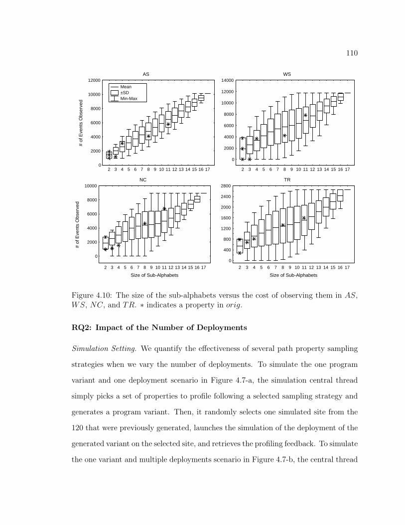
110
AS
2 3 4 5 6 7 8 9 10 11 12 13 14 15 16 170
2000
4000
6000
8000
10000
12000#
of E
vent
s O
bser
ved
Mean ±SD Min-Max
WS
2 3 4 5 6 7 8 9 10 11 12 13 14 15 16 17
0
2000
4000
6000
8000
10000
12000
14000
NC
2 3 4 5 6 7 8 9 10 11 12 13 14 15 16 17
Size of Sub-Alphabets
0
2000
4000
6000
8000
10000
# of
Eve
nts
Obs
erve
d
TR
2 3 4 5 6 7 8 9 10 11 12 13 14 15 16 17
Size of Sub-Alphabets
0
400
800
1200
1600
2000
2400
2800
Figure 4.10: The size of the sub-alphabets versus the cost of observing them in AS,WS, NC, and TR. ∗ indicates a property in orig.
RQ2: Impact of the Number of Deployments
Simulation Setting. We quantify the effectiveness of several path property sampling
strategies when we vary the number of deployments. To simulate the one program
variant and one deployment scenario in Figure 4.7-a, the simulation central thread
simply picks a set of properties to profile following a selected sampling strategy and
generates a program variant. Then, it randomly selects one simulated site from the
120 that were previously generated, launches the simulation of the deployment of the
generated variant on the selected site, and retrieves the profiling feedback. To simulate
the one variant and multiple deployments scenario in Figure 4.7-b, the central thread

111
launches the simulation of the program variant’s deployment to 60 and 120 generated
sites in their own site-threads (the value of 60 deployments is chosen to enable finer
observation of the trends in varying the number of deployments).
We evaluate two sampling strategies: basic and path. The basic strategy randomly
selects a set of properties while the path strategy favors properties that provide the
most diverse acyclic trap strings. For each strategy, we use two property sampling
spaces: orig and lat. This yields four sampling techniques: basic-orig and path-orig
strategies select the profiled properties from the original set of properties; and basic-
lat and path-lat techniques select them from the lattice of sub-alphabet properties.
We use the sampling strategies to select a set of properties to be profiled while
satisfying the 1%, 5%, 10%, 15%, and 20% overhead bounds. To account for the
degree of randomness in the property selections and the user sites assignments, we
performed this process 10 times. Figure 4.11 provides a summary of our findings in the
form of box plots for each of the techniques. (We append the number of deployments
behind the techniques name. For example: path-lat-120 refers to path-lat strategy
with 120 deployments.)
Result Analysis. Increasing the number of deployments increases the number of
violations detected. This is to be expected since increasing the number of deploy-
ments means that we expose the program variant to more, and potentially richer,
program behavior, increasing its chance to detect more violations. However, this
benefit diminishes as the number of deployments increases and the overhead bound
increases. For example, with the path-lat strategy with an overhead bound of 15%,
increasing the number of deployments from one to 60 allows us to detect 10 more
violations. However, increasing the number of deployments from 60 to 120 with the
same strategy only detects five more violations.
Independent of the profiling overhead bound and number of deployments, sam-

112
1%
0
5
10
15
20
25
30
35#
of V
iola
tions
Det
ecte
d Mean ±SD Min-Max
5%
0
5
10
15
20
25
30
35
10%
basi
c-or
ig-1
basi
c-la
t-1
path
-orig
-1
path
-lat-
1
basi
c-or
ig-6
0
basi
c-la
t-60
path
-orig
-60
path
-lat-
60
basi
c-or
ig-1
20
basi
c-la
t-12
0
path
-orig
-120
path
-lat-
120
Sampling Techniques
0
5
10
15
20
25
30
35
# of
Vio
latio
ns D
etec
ted
15%
basi
c-or
ig-1
basi
c-la
t-1
path
-orig
-1
path
-lat-
1
basi
c-or
ig-6
0
basi
c-la
t-60
path
-orig
-60
path
-lat-
60
basi
c-or
ig-1
20
basi
c-la
t-12
0
path
-orig
-120
path
-lat-
120
Sampling Techniques
0
5
10
15
20
25
30
35
20%
basi
c-or
ig-1
basi
c-la
t-1
path
-orig
-1
path
-lat-
1
basi
c-or
ig-6
0
basi
c-la
t-60
path
-orig
-60
path
-lat-
60
basi
c-or
ig-1
20
basi
c-la
t-12
0
path
-orig
-120
path
-lat-
120
Sampling Techniques
0
5
10
15
20
25
30
35
# of
Vio
latio
ns D
etec
ted
Figure 4.11: Violation Detection vs Number of Deployments

113
pling over the space of lat consistently resulted in the detection of more violations
than sampling over orig. This was more obvious with higher overhead bounds. For
example, with an overhead bound of 20%, with 120 deployments and sampling with
the path strategy, the difference in performance between lat and orig is up to four
violations (10% increase). As the overhead bounds get tighter, the differences among
sampling strategies decrease because the number of properties fitting the overhead
constraint is reduced. Furthermore, under extreme overhead constraints, the popula-
tion of selectable properties is small enough that sampling strategies cannot make a
difference.
When we compare more complex sampling strategies, i.e., path strategies, with
basic, we note that path strategies are able to detect more violations than basic.
With an overhead bound of 20% and 120 deployments, path detects an average of up
to 10 more violations than basic. As observed before, however, the benefits decrease
under tighter profiling overhead bounds (using path leads to the detection of only four
additional violations when the overhead bound is 5%). The box plots also reveal that
the most advanced sampling strategy provides smaller violation detection variability
(smaller boxes). This is beneficial because their performance is more consistent and
can be better estimated than the basic strategy.
Implications. The gain in violation detection power obtained by increasing the
number of deployments confirms our belief in the potential of deployed profiling, where
it facilitates the program’s exposure to a richer set of behaviors. Providing a richer
space to sample from can reinforce this gain, but only when the overhead bound is not
too restrictive. If we can generate only one program variant, the choice of sampling
strategy is not important as the diversity that one can obtain from the sampled set is
very limited.

114
RQ3: Impact of the Number of Variants
Simulation Setting. To evaluate the effectiveness of the sampling strategies under
different numbers of variants, we use the same four sampling strategies and overhead
bounds as in RQ2 to select 120 sets of properties, where each set of properties is used
to generate one program variant, and each variant is deployed to a site. To simulate
the multiple variants (across deployments) and multiple deployments scenario in Fig-
ure 4.7-c, for each program variant, the simulation central thread randomly selects,
without replacement, a deployment site to become the target of the deployment, and
launches the selected user site’s thread. Similar to RQ2, we account for the random-
ness of the property selection and site assignment by performing the process 10 times.
We plot the average of the total number of violations detected across the number of
program deployments generated as a line graph in Figure 4.12. (Note that in this
scenario, we create a new variant for each deployment, hence the number of variants
and deployments are the same.) To ease the comparison with the one variant and
multiple deployments scenario of Figure 4.7-b, we also plot, in this figure, the average
value of the four sampling strategies from Figure 4.11 at 60 and 120 deployments.
(Note also that the y-axis scalings for 1% and 5% bounds are smaller than the other
bounds in order to show the differences in the one variant values more clearly.)
Result Analysis. We can observe that increasing the number of variants generated
also increases the number of violations detected. This benefit is more apparent for
higher overhead bounds. For example, at the 1% overhead bound, the increase in
the violations detected from one generated program variant to 120 program variants
is about two violations across the different sampling techniques. However, at the
20% overhead bound, the increase is up to 20 violations for our most sophisticated
sampling technique (path-lat).
When compared to the one variant and multiple deployments scenario, we can ob-

115
1%
1 11 21 31 41 51 61 71 81 91 101 111 1210
2
4
6
8
10
# of
Vio
latio
ns D
etec
ted
5%
1 11 21 31 41 51 61 71 81 91 101 111 1210
5
10
15
20
25
10%
1 11 21 31 41 51 61 71 81 91 101 111 121
# of Deployments/Variants
0
5
10
15
20
25
30
# of
Vio
latio
ns D
etec
ted
15%
1 11 21 31 41 51 61 71 81 91 101 111 121
# of Deployments/Variants
0
5
10
15
20
25
30
20%
1 11 21 31 41 51 61 71 81 91 101 111 121
# of Deployments/Variants
0
5
10
15
20
basic-orig basic-lat path-orig path-lat 25e
30
35
# of
Vio
latio
ns D
tect
ed
basic-orig (1 variant) basic-lat (1 variant) path-orig (1 variant) path-lat (1 variant)
Figure 4.12: Violation Detection vs Number of Variants (and Deployments)

116
serve that more violations can be detected by generating additional program variants
assigned for each deployment. At the 10% overhead bound, for path-lat, deploying
one variant to 60 user sites (marked by a triangle in Figure 4.12) can detect, on av-
erage, 11 violations. Meanwhile, generating 60 variants, where each is deployed to
a distinct user site can detect up to 13 violations. Increasing the number of deploy-
ments (and the assigned new variants) to 120, at this overhead bound, still yields a
difference of up to two violations.
More interestingly, however, is that at higher bounds, the benefit of generating
60 variants, instead of one, and deploying it to 60 sites is more apparent than when
120 deployments are used with just one variant. This means that a larger number of
deployments may not overcome the limitation of a variant or even a set of variants.
This also suggests that generating more program variants can compensate for the lack
of deployed sites.
At the 1% overhead bound, similar to RQ1, we can observe that all the techniques
detect a small fraction of the violations. We conjecture that most of the violation
revealing properties cost more than 1% when profiled, hence none of the techniques
are able to select these properties. For overhead bounds of 5% and 10%, the violation
detection rates of the techniques flatten at around 10 and 15 violations respectively.
However, at higher overhead bound values, such as at 15% and 20%, the growth
is accelerated, suggesting that at higher overhead bounds, most violations can be
detected with fewer deployments.
Regardless of the overhead bound, we can observe that strategies that select the
properties from orig generally have lower detection rates than ones that select from
lat. This difference is more obvious for higher overhead bounds. This is because at
higher overhead bounds, the sampling strategies that utilize the lattice of properties
have more options regarding which properties to select when compared to ones that

117
utilize the orig set of properties.
Implications. Increasing the number of variants generated allows the profiling of
more properties, hence increasing the violation detection ability. Additionally, if the
number of deployed sites available is limited, increasing the number of variants can
compensate for this limitation. The increase in the number of profiled properties
requires sampling strategies that can provide diversity in the sampled set. The richness
of the lattice sampling space can help to provide such diversity.
RQ4: Impact of Sampling Refinements
Simulation Setting. For the multiple variants and multiple deployments scenario in
Figures 4.7-c, 4.7-d, and 4.7-e, the main simulation thread generates 120 program
variants and simulates each variant’s deployment to one of the 120 sites. In the case
of variant generation across time scenarios (Figures 4.7-d and 4.7-e), after the field
data is received, the site-thread places a new request to receive another variant. A
site-thread notifies the central thread when: (1) a violation is detected, or (2) the
execution of the test suite, simulating a site behavior, is completed. The central-
thread continues deploying sites until all violations are detected or an upper bound
of 2400 program variants have been deployed. This corresponds to deploying 20
variants at each user site. This number was selected because we observed that after
20 iterations, either all of the seeded violations have been detected or the rate of
detection of new violations had flattened.
To answer the research question, we use the simulation tool to select a new set
of properties to monitor whenever a deployment request is received using one of
the four techniques described in Table 4.4 (all of the strategies are applied to lat

118
Sampling Technique Sampling Strategy performed on Latticebasic-lat Randomly selects profiled properties.path-lat Selects properties that provide most diverse trap stringspath-lat-global-feedback Selects properties with the highest weight and that provide
the most diverse trap strings, where the weighting scheme isadjusted globally.
path-lat-local-feedback Selects properties with the highest weight and that providethe most diverse trap strings, where the weighting scheme isadjusted globally and locally.
Table 4.4: Summary of the sampling techniques.
since it consistently outperforms orig). Note that in this scenario, the basic and
path strategies represent resampling techniques that do not utilize a feedback loop
(i.e., the scenario shown in Figure 4.7-d). Meanwhile path-lat-global-feedback and
path-lat-local-feedback correspond to the resampling techniques that utilize feedback
(i.e., the scenario in Figure 4.7-e). To account for randomness in our simulation and
sampling strategies, we performed 10 runs, each with a new set of 120 deployed sites,
and reported the average number of deployments needed to detect all violations in the
line plots shown in Figure 4.13. Note that we only show the line plots for overhead
bounds of 1%, 5%, and 10% (the trends for 15% and 20% are similar to those of 10%).
Result Analysis. At the 1% overhead bound, none of the techniques are able to de-
tect all violations before the bound of resampling (20 iterations) is reached. However,
both of the feedback-based techniques, path-lat-global-feedback and path-lat-local-
feedback, are able to detect up to two new violations after about 400 program variants
are monitored (3-4 sampling cycles per site). This confirms our conjecture that most
of the seeded violations require profiling for more expensive properties to be detected.
At 5% and 10% overhead, it is more obvious that there is a significant benefit
from continuously re-sampling the program properties and generating program vari-
ants over the profiling activity. At 5% overhead, using the path-lat technique, we
can detect 10 violations by generating and deploying 120 program variants. Through

119
1%
112
124
136
148
160
172
184
196
110
8112
0113
2114
4115
6116
8118
0119
2120
4121
6122
8124
01
0
5
10
15
20
25
30
35
# of
Vio
latio
ns D
etec
ted
basic-lat path-lat path-lat-global feedback path-lat-local feedback
5%
112
124
136
148
160
172
184
196
110
8112
0113
2114
4115
6116
8118
0119
2120
4121
6122
8124
010
5
10
15
20
25
30
35
# of
Vio
latio
ns D
etec
ted
10%
112
124
136
148
160
172
184
196
110
8112
0113
2114
4115
6116
8118
0119
2120
4121
6122
8124
01
# of Variants
0
5
10
15
20
25
30
35
# of
Vio
latio
ns D
etec
ted
Figure 4.13: Rate of Violation Detection for Refinement With and Without feedback

120
resampling and redeploying each of the program variants, we are able to detect 26
additional violations (one violation remains undetected) after more than 2000 vari-
ants. At 10% overhead, the technique is able to detect all violations after generating
about 1500 program variants.
When comparing the techniques’ performance, we observe that basic-lat (the solid
line in the figure) has the lowest detection rate of all techniques. At 5% overhead, the
detection rate seems to plateau after 1800 program variants have been deployed.
At 5% and 10% overhead, path-lat, path-lat-global-feedback, and path-lat-local-
feedback have similar detection rates during the first iterations. However, after the
easiest violations are detected, path-lat starts to loose its effectiveness when compared
to the two feedback-based strategies.
Overall, both of the feedback-based techniques perform better than the path-lat
technique. Moreover, path-lat-local-feedback has the highest violation detection rate;
when the overhead bound is at 5%, it is able to discover 100% of the path property
violations when basic-lat, path-lat, and path-lat-global-feedback found 45%(17), 56%
(21), and 86%(32) of the violations respectively. The advantage of the feedback-based
strategies, however, diminishes as the overhead bound increases since more expensive
and potentially powerful properties can be profiled in each variant.
Implications. If timeliness detection of a violation is not a priority or if profiling
feedback is not available, the repeating property should be used to increase the viola-
tion detection. Refining the sample of profiled properties through the use of feedback,
however, enables more (unique) violations to be detected and at a faster rate.

121
4.6 Conclusions and Future Work
We introduced a novel approach for controlling the overhead cost of profiling path
properties by composing a single integrated property from a set of simpler and smaller
properties, decomposing it into a set of sub-alphabet properties that collectively pre-
serves the integrated property’s violation detection power, and then strategically sam-
pling a subset of these properties to enable profiling under tight overhead constraints.
Additionally, we introduced a lattice weighting scheme that associates each property
with a weight and showed how we can use the weights value to incorporate profiling
feedback and further improve the chances of detecting currently undetected violations.
We conducted several studies, evaluating the lattice-based sampling approach un-
der several deployment scenarios. Our results showed the potential of our approach
to detect more path violations with less overhead when compared to profiling the
original properties. However, the rich diversity in the violation detection power, size
of sub-properties alphabets, profiling cost, and the frequency of the properties in the
lattice with specific characteristics prompts the need for smarter sampling schemes.
For all deployment scenarios and overhead constraints, our proposed sampling
strategies are able to select properties that yield higher violation detections than when
randomly sampling across properties. When increasing the number of program vari-
ants, the number of violations detected also increased and the benefit from employing
more sophisticated sampling strategies was more apparent. A similar trend was also
observed when the number of deployments was increased. Finally, our study revealed
that refining the profiling activity through resampling of the profiled properties al-
lows for higher violations to be detected. Moreover, the feedback-based sampling
strategies are able to detect more violations at a faster rate than the non-feedback
based strategies and the performance can be improved by leveraging local feedback
to further adjust the weighting scheme.

122
In the future, we want to perform further studies to evaluate the effectiveness
of our approach over other path properties including properties involving dynamic
object creation such as enumeration. Profiling such properties is difficult because
the allocated objects tend to be short lived and constrained to a small number of
method calls, but they occur with high frequencies. Dynamic objects, however, are
commonly found in many Java programs, and have many interesting properties [9, 10].
We also wish to explore other forms of feedback apart from coverage vectors and to
investigate the trade-offs between the cost of capturing additional information and
its effectiveness in guiding the feedback-based sampling strategies. Finally, we are
interested in incorporating static analysis to enrich the obtained profiling observation.
For example, flow analysis may be employed to determine if observing a property
inherently means a more expensive property was also observed.

123
Chapter 5
Trace Normalization0
In Chapters 3 and 4 we have discussed two techniques that can be applied at a
pre-deployment phase to reduce and control the profiling overhead and enable the
capturing of field traces. At a post-deployment phase, the profiled traces can be
utilized to perform dynamic analyses. The strength of many dynamic analysis tech-
niques depends heavily on the variability of the pool of traces they operate on. A
richer trace pool can result, for example, in improved sets of inferred invariants [34],
more precise fault isolation [19], and smaller change impact sets [49]. On the other
hand, trace variability may be detrimental when it introduces noise, i.e., variation
in traces that is not related to the program’s properties or characteristics that we
wish to analyze. Profiling deployed software can yield large number of traces that are
richer and more diversified. However, field traces can potentially contain noise within
them, that is intensified with their volume.
Existing techniques, as described in Section 2.3, have addressed the problem of
identifying the interesting execution traces at a post-deployment by proposing tech-
niques to cluster execution traces, and then sample from these clusters [13, 22, 39, 51].
0Some of the work in this chapter has been previously published in [25].

124
The underlying assumption is that the traces that are further apart (placed in dif-
ferent clusters) are more likely to contain distinct information valuable to a client
analysis. This basic assumption, however, may not always hold. We define an execu-
tion trace as a record of the sequence of events (e.g., as statement executions, method
executions, menu’s items, user’s actions, or user’s inputs) that occurred during a pro-
gram execution. Traces may end up in different clusters due to irrelevant variations
in the sequences of events that comprise them and make them appear different, and
therefore valuable, even though the observed variation is unrelated to the program
property under analysis. This can lead to the retention of a trace that provides no
added value relative to a given trace pool.
We identify two sources of irrelevant variations. The first source are trace events
whose occurrence can be re-ordered (commuted) without affecting the program state.
For example, in a web browser, the events for changing a password and setting one’s
homepage affect different variables or fields in the program. The second source of ir-
relevant variations are redundant events whose occurrence does not lead to a distinct
program state and can be collapsed. A trivial instance of redundant events are exe-
cutions of inspector methods (i.e., methods that are responsible to display the value
of a program’s variables or data structures). Our work aims to reduce the irrelevant
variations of trace events through a normalization that attempts to preserve the dis-
tinct structure of traces while eliminating differences due to commuted or collapsed
sub-traces.
5.1 A Motivating Example
We start by illustrating how a fault isolation client analysis works, and how it would
benefit from our trace normalization approach.

125
public class XMLElement { ...private Vector children;private String name;private String content;
}public class Builder { ...
private XMLElement root;}public class Parser { ...
protected void processEle() { // Processes a regular element....// if statement is faulty – the operator || should be &&if ((ch == ′ <′) || (! fromEntity[0]))
...this.builder.endElement(...);
else(...)...this.builder.addPCData(true);
...} }public class Valid {
protected Hashtable attValues;protected Hashtable entities;...public void parseDTD() { ... // Parses the DTD.
for(...) { ...if (...)
this.processEnt(true);else if (...)
this.processAtt(true);...
} }
Figure 5.1: A snippet of NanoXML Program
Many fault isolation analyses compare traces of passing and failing program runs,
and use their differences to pinpoint a likely fault’s location. The fault isolation
analysis we study here is one instance of that type of analysis; it was introduced by
Dallmeier et al. [21] to perform lightweight bug localization by assigning a score to
each class based on its probability of containing the fault. In our example, a class
score is calculated by counting the number of method call sequences, initiated in that
class, that differentiate passing runs from a failing run.
Consider the two classes StdXMLParser and NonV alidator (later referred to as

126
…, v.parseDTD, v.processEnt, r, v.processAtt, r, …, p.processEle, b.addPCDATA, r, r, …
…, v.parseDTD, v.processAtt, r, v.processEnt, r, …, p.processEle, b.endElement, r, r, …
tp
tf
tp
tf
v.processEnt - r - v.processAtt - r
v.processAtt, r, v.processEnt, r
…, Util.read, Util.scanEntity, return, return, …, Parser.processElement, Builder.addPCDATA, return, return, …
…, Util.read, Util.scanEntity, return, return, …, Parser.processElement, Builder.endElement, return, return,
tp
tf
a. Traces
b. Program States
c. Segments
d. Commutative Transformation
e. Normalized Traces
v.processEnt , r, v.processAtt, r
…, v.parseDTD, v.processAtt, r, v.processEnt, r, …, p.processEle, b.addPCDATA, r, r, …
…, v.parseDTD, v.processAtt, r, v.processEnt, r, …, p.processEle, b.endElement, r, r, …
attValuesentities
root
Page, 0 null null
Page, 0 Writer,w null
Page, 0 Writer,w db:null → null
Page, 0 Writer,w db:null → null
Page, 0 Writer,w db:null → null
attValuesentities
root
null null null
v.processAtt - r - v.processEnt - r Page, 0 Writer,wnull
null null null
null null null
Page, 0 Writer,w null
null Writer,w null
Page, 0 Writer,w db:null → null
Page, 0 Writer,w db:null → name:null
Page, 0 Writer,w db:null → name:foo
Si Se
Figure 5.2: Trace Normalization approach steps applied to the example.
Parser and V alid for brevity) shown in Figure 5.1 of NanoXML, a software artifact
we study later in Section 5.4. Note that the Parser class has a seeded fault in a
predicate within the processEle method. Given Parser p, V alid v, and Builder b,
suppose that two executions of NanoXML lead to the generation of the two traces in
Figure 5.2-a composed of method invocations and returns, r, where tf corresponds to
a failing run and tp to a passing run.
Let us assume that we consider only call sequences using a sliding window of size
2. Table 5.1 shows the method call sequences that correspond to the traces tp and
tf . Trace tp contains the call sequences v.parseDTD - v.processEnt, v.processEnt
- v.processAtt and p.processEle - b.addPCDATA. Meanwhile, tf contains the call se-

127
Table 5.1: Class score for fault isolation analysis performed on original traces.Class Sequence Set of tp Sequence Set of tf Score
Valid v.parseDTD - v.processEnt v.parseDTD - v.processAtt 4v.processEnt - v.processAtt v.processAtt - v.processEnt
Parser p.processEle - b.addPCDATA p.processEle - b.endElement 2
quences v.parseDTD - v.processAtt, v.processAtt - v.processEnt and p.processEle
- b.endElement. Given this setting, Dallmeier et al.’s fault isolation client anal-
ysis will assign a score of four to the V alid class because sequences v.parseDTD-
v.processEnt and v.processEnt-v.processAtt appear in tp but not in tf , and
v.parseDTD-v.processAtt and v.processAtt-v.processEnt appear in tf but not
in tp. The same process leads to a score of two for the Parser class, which means
that the V alid class is more likely to contain the fault than the Parser class, even
though the fault is in Parser.
Although not immediately obvious, the above traces contain irrelevant variations
to the fault isolation analysis that cause this client to return an imprecise score
value, skew the class rankings, and potentially provide a larger set of fault locations
for a developer to explore. We now illustrate how our approach can identify those
irrelevant variations, and normalize the traces to reduce them, improving the fault
isolation client effectiveness.
Our Trace Normalization Approach
Our approach requires the capture of one additional piece of information: program
state. We discuss the different forms of program state that may be captured shortly,
but for this example, assume that the relevant program state we capture for this
program and analysis consists of:
1. The root variable of the Builder class representing the structure of the parsed
XML (this key data structure is implemented by the XMLElement class in

128
Figure 5.1).
2. The hashtables containing the XML DTD Attributes (attV alues) and Entities
(entities) information.
This capture is performed at the end of each method return as illustrated in Figure
5.2-b. In our example, after the last event in trace tp, the program state captured
shows one entry in the entities hashtable, one entry in the attV alues hashtable, and
a root XML element named db which has one child element. The child element has
the value name as its name and the value foo as its content with no other children.
Given the traces and the captured program states, our approach consists of three
steps. First, we identify segment sets within the traces, where a segment set contains
event sequences within traces that are bounded by the same program states, Si and
Se. The event sequences bounded by Si and Se are called segments. We observe in
Figure 5.2-c that at least one segment set can be identified from the two traces which
contains the segments:
〈v.processEnt, r, v.processAtt, r〉
〈v.processAtt, r, v.processEnt, r〉
where the Si and Se are marked with bolded squares.
Second, we identify irrelevant variations in each segment set. The identification is
based on the observation that segments in a segment set start in the same Si, and in
spite of including different sequences of events, end up in the same Se. Hence, parts
of those event sequences may constitute irrelevant variations. We target variations
due to commutative events or event sequences, and collapsible event occurrences.
Informally, we allow two events (or event sequences) to commute within a segment
set when those events have appeared in different orders in at least two segments from
that set. A sequence of events in a segment is collapsible if it can be reduced in length

129
to match another segment. For our example, we note in Figure 5.2-d that the two
segments contain an irrelevant variation caused by commuting the v.processEnt-r
and v.processAtt-r events.
The last step, Figure 5.2-e, is to normalize the segments in each segment set.
Normalization involves transforming each segment to order commutative events in a
canonical order and to collapse sequences of repeated events to a minimal length. The
normalization process operates in a greedy manner: each trace and its corresponding
program states are parsed to identify an Si for a segment. When such an Si is found,
we look for the first Se such that there exists at least one irrelevant variant that
can be normalized in the segment bounded by states Si and Se. Then we apply the
normalization operations as defined previously. The process continues from Si to find
another segment until it reaches the end of the trace.
Continuing with our example, we may decide that all occurrences of
〈v.processEnt, r, v.processAtt, r〉
should be normalized to
〈v.processAtt, r, v.processEnt, r〉
As shown in Figure 5.2-e, one instance of this normalization can be applied in tf .
Table 5.2 presents the method call sequences produced using the normalized traces.
When considering this normalized version of tf , since the V alid class contains the
call sequences v.parseDTD-v.processEnt and v.processEnt-v.processAtt in both
Table 5.2: Class score for fault isolation analysis performed on normalized traces.Class Sequence Set of tp Sequence Set of tf Score
Valid v.parseDTD - v.processAtt v.parseDTD - v.processAtt 0v.processAtt - v.processEnt v.processAtt - v.processEnt
Parser p.processEle - b.addPCData p.processEle - b.endElement 2

130
traces, the fault isolation technique assigns it a score of zero. Meanwhile, the two
differentiating call sequences for Parser remain unchanged in the presence of the
normalized traces, which means that it would still have a score of two, making Parser
more likely than V alid to contain a fault. Given the fault location, we see how the
normalized traces enhance the precision of the fault isolation client analysis.
5.2 Background and Definitions
Section 5.1 introduced the concepts of segments, segment sets, and commutative and
collapsible events, which form the basis of our trace normalization approach. We
define them more precisely here. Then, we discuss the application and some trade-
offs of our approach.
5.2.1 Key Concepts: Commutative and Collapsible
Intuitively, a trace segment defines a region of program execution that transits from
an initial program state, Si, to an ending program state, Se. Collecting such seg-
ments and analyzing their similarities and differences is the foundation of trace nor-
malization. Segments are sub-traces consisting of at least two events bounded by a
designated pair of states (for commutativity and collapsibility to be applicable).
Definition 5.2.1 (Segment) Given two program states Si and Se, a trace t con-
sisting of a vector of events, e ∈ Σ, has a segment 〈SiβSe〉, if t = αSiβSeγ, where
α, γ ∈ Σ∗ and β ∈ Σk where k > 1.
Segment sets are non-singleton sets of segments bounded by common program
states. Note that a segment set can contain multiple segments belonging to just one
trace.

131
Definition 5.2.2 (Segment Set) Given two program states Si and Se and a set of
traces T ,
SEGSETSi,Se = {〈Siβ1Se〉, ..., 〈SiβmSe〉}
s.t m > 1 ∧ ∃t ∈ T : 〈SiβjSe〉is a segment of t
The identification of irrelevant variations is based on the notion of commutative
and collapsible events.
Definition 5.2.3 (Commutative Events) Two events, A and B, commute in
SEGSETSi,Se if:
∃s ∈ SEGSETSi,Se∃α, β, γ ∈ Σ∗ : s = 〈SiαAβBγSe〉
∃{s′1, ..., s′m} ∈ SEGSETSi,Se∃{α′
1, ..., α′m}, {β′
1, ...β′m}, {γ′
1, ..., γ′m} ∈ Σ∗ :
∀j < m, s′j = 〈Siα′jBβ′
jAγ′jSe〉
This definition requires that for events A and B to commute within a segment
set, both A and B should appear in at least m + 1 segments in the set with differing
orders. It is worth noting that this definition allows arbitrary freedom in matching
a common prefix, infix, and suffix of the commuting events within a segment. This
definition can be easily extended for fixed sequences of events by replacing A with
a1, . . . , aj and B with b1, . . . , bl.
Definition 5.2.4 (Collapsible Events) A sequence of consecutive occurrences of
event A, Ak where k > n, is collapsible to An, 1 < n < k, within a segment set
SEGSETSi,Se if:
∃{s1, ..., sm} ∈ SEGSETSi,Se, {α1, ..., αm}, {γ1, ..., γm} ∈ Σ∗ :
∀j < m, 〈SiαjAnγjSe〉 ∈ SEGSETSi,Se
132
Similar to Definition 5.2.3, Definition 5.2.4 require the existence of at least m +
1 segments within a set with the desired property. For both Definition 5.2.3 and
Definition 5.2.4, a more relaxed notion of normalization simply requires a smaller m.
5.2.2 Approach Applicability and Trade-offs
A dynamic client analysis (DA), such as the fault isolation analysis discussed in
Section 5.1, requires the program under analysis P to be instrumented to log events
Σ. As the program is executed, a set of traces T = {t1, t2, . . . , tk} is collected,
where trace ti is a vector of events, e ∈ Σ, captured during one execution of P . In
general, a DA operates on T to calculate properties of P (e.g., invariants in P ) or
P ’s components (e.g., fault likelihood of P ’s classes). For simplicity, we consider only
program events that correspond to method calls.
Conceptually, our normalization approach aims to transform the traces in T to
obtain a new trace set T ′ such that the DA(T ′) is more precise than DA(T ) and
DA(T ′) has recall that is at least that of DA(T ). We can define precision and recall
following the notion in information retrieval. Precision refers to the ability of the
dynamic analysis in providing results that are truly relevant to the analysis. In other
words, DA(T ′) is more precise than DA(T ) if it reports less number of false positives.
On the other hand, recall refers to the ability of the analysis in retaining the truly
relevant results.
The specific formulation of precision and recall, however, will depend on the DA.
For the fault isolation technique, it is natural to compare techniques based on the
extent to which the class ranking produced increases the ease with which a fault is
found. To accommodate this type of rank comparison, we set a precision threshold by
considering only the top X classes in the ranking as the information produced by the
analysis. A technique has 100% recall if the faulty class is within the top X classes.

133
For other client analyses, the formulation of precision and recall will be different. For
example, the dynamic change impact analysis presented in Section 5.4 identifies sets
of methods affected by a program change. Consequently, its precision is improved
by eliminating information from T that allows it to report fewer methods that are
not impacted by the change. It retains the recall of the original analysis as long as
it reports at least as many actual changed methods. We provide a more detailed
formulation of precision and recall for fault isolation and dynamic impact analysis in
Section 5.4.
Identifying transformations that can increase precision while retaining recall is
challenging. Our approach discriminates trace variations that do not contribute to a
DA’s recall from those that add irrelevant variations that reduce DA’s precision. It
performs this discrimination by identifying alternative event sequences (bounded by
the same program states) that differ in the number or in the order of their events.
We note that while our goal is to retain recall, there may be situations in which it is
acceptable to sacrifice some recall to significantly increase precision. This is especially
true when precision is achieved by greatly reducing the size of the trace pool or the
amount of spurious information produced by the analysis.
In addition to precision and recall, an assessment of trace normalization must
consider the cost of capturing program states 〈si,1, ..., si,j, ..., si,m〉 for each trace
ti, where si,j is the program state generated by ti at checkpoint j. A program state can
be viewed as an n-tuple of memory values, where each value corresponds to a “state”
of a program’s component, and a program’s component can be a scalar variable,
a reference variable such as an object, a thread, or a program location. Clearly,
if not done carefully, capturing program states during an execution may introduce
significant overhead in the data collection. We discuss several mechanisms to control
this overhead cost in Section 5.4.4

134
In the end, the choice of what program states to capture and when to do it in-
volves balancing the cost of data collection and processing, the potential benefits of
normalization, and the implications for the precision and recall of client analyses.
Capturing a more complete program state, for example, may result in a more precise
analysis, but would also require more expensive data collection and processing, and
lead to the identification of fewer segment sets and fewer opportunities for normal-
ization. We believe that there are opportunities to reduce the cost of normalizing a
trace pool across different client analyses by choosing and abstracting parts of the
program state that contain at least as much information as those required by client
analyses.
In addition to the program states, the normalization approach itself may sacri-
fice recall in order to significantly reduce the irrelevant variations in a trace pool, and
consequently improve the precision of a client analysis. For example, the most restric-
tive application of commutative event sequences requires for the candidate segments
to have identical suffixes, prefixes, and infixes. Such constraints can be relaxed to
enable a more aggressive normalization that gains precision but may sacrifice recall.
Overall, the choice of which parts of program state to capture, and what normal-
ization operations and how they are applied to reduce trace segments, will influence
the precision and recall of an analysis operating on the reduced trace pool. Still, as we
shall see in our study of two client analyses that operate on traces with method call
and return information, the normalized traces retained most if not all of the recall,
achieved greater or equal precision, and reduced client analysis cost.

135
Comparison mechanisms
Sensitivity Control
Trace + Program
State
Segment Sets
State Identifier
Analyzer Sets of SegSet
Variations
Trace Normalizer
Client Analysis
Matching States
Decomposer
Pool of Traces + Program
States
Normalized Pool of Traces
Phase 1 Phase 2
prefix infix suffix
Figure 5.3: Trace Normalization Infrastructure.
5.3 Trace Normalization Infrastructure Support
We have built an infrastructure to support trace normalization that allows us to
explore several aspects of the approach. Figure 5.3 provides an overview of the in-
frastructure which operates in two phases. The first phase involves the state identifier
and decomposer components. These components incrementally process one trace at
a time, generating a collection of segment sets from a pool of traces and program
states. In the second phase, these segments sets are processed by the analyzer and
the normalizer to transform the original pool of traces by removing their irrelevant
variations. We now discuss the infrastructure in more detail.
5.3.1 State Identifier
The state identifier determines a set of candidate program states that may demark
the beginning (Si) or the end (Se) of segments within traces. The state identifier

136
takes a pool of traces and their associated program states, and generates a map from
a program state to a pair consisting of a trace identifier and a set of offsets within
that trace. The offsets encode the locations within the trace that correspond to the
checkpoints in which the program state is captured. To do this, traces are scanned
and whenever a candidate state is found, either new entries in the map are created
or existing entries are updated with new trace and offset values. The map entries of
candidate states that do not appear in multiple traces or locations cannot be segment
delimiters, so they are deleted.
5.3.2 Decomposer
When presented with a trace pool and the program state-trace map provided by
the state identifier component, the decomposer utilizes Definitions 5.2.1 and 5.2.2
to construct the segment sets: for every pair of states, Si and Se, in the map, the
decomposer looks for all the traces in which both of the states appear. Then, for each
such trace, the decomposer considers the event segments bounded below by Si and
bounded above by Se (which is identified by stored offsets in the map), and adds the
segment to the SEGSETSi,Se only if the length of the segment is greater than one.
An unoptimized implementation of the decomposer may be quadratic in the num-
ber of non-trivial program states and in the length of a trace; and linear in the number
of traces. Again, we defer discussion on how we can mitigate this problem to Section
5.4.4.
5.3.3 Analyzer
For each segment set the analyzer uses Definitions 5.2.3 and 5.2.4 to identify patterns
that expose potential sources of irrelevant variation among its segments. Specifically,
we identify commutative events and collapsible events within segments. The analyzer

137
can be configured to infer only the commutative properties, the collapsible properties,
or both.
Note that the two definitions allow the analyzer to be configured through the
parameters that define the desired length of common prefix, infix, and suffix of the
commuting events within the segments in a segment set. The length of prefix, infix,
and suffix determine how conservative the approach will be in terms of normaliz-
ing the potentially irrelevant sequence variations. Generally, increasing the length of
matching sequences will lead to the identification of less irrelevant variations. How-
ever, it may also mean less spurious irrelevant variations. In our implementation, we
vary the value of the prefix and suffix lengths when evaluating our approach. We set
the length of infixes for commutative variations to zero to ensure that only adjacent
events are considered to be commutative.
When inferring the commutative and collapsible variations within a segment set,
there is also some flexibility in the required number of segments in the set that exhibit
the potentially irrelevant patterns. Intuitively, the greater the number of segments
in a set that contain a pattern, the more confident one might be that the pattern is
truly irrelevant. For example, if half of the segments have an A followed by a B and
half of the segments have them in reverse orders, then we can be confident about the
commutativity of A and B. In our study, we did not explore this type of variation.
Instead, we used Definitions 5.2.3 and 5.2.4 as stated.
5.3.4 Trace Normalizer
This component generates a normalized version of a trace by utilizing the original
trace and the set of variations associated with each segment set provided by the
analyzer. The normalizer parses the trace and its corresponding program state for
a trace segment, attempting first to identify an Si. When such an Si is found, the

138
normalizer scans forward for the first Se such that there exists at least one irrelevant
variation that can be normalized in SEGSETSi,Se . Only the irrelevant variation that
is identified within this segment set can be applied to the corresponding segment.
The normalizer will then attempt to perform the transformation process.
The transformation process based on commutative events selects an order of those
events and transforms each segment in the set so that occurrences of those events
within that segment set obey that order. Certain ordering heuristics, such as sorting
the instances of the segment variations and always choosing the first instance of an
event sequence as the canonical one for commuting operation, should be applied to
maintain the consistency of the normalization operations (we use a canonical ordering
in our implementation). Applying the transformation process on the collapsible events
selects the shortest sequence of repeated events in a segment set and replaces all longer
sequences in segments in the set with it.
Once all possible variations are normalized within the segment, the normalizer
looks for a new potential Si from Se and restarts the process. Once the target trace
is normalized, a string comparison is performed against the other already-reduced
traces to avoid duplication.
5.4 Empirical Study
This study investigates the performance of our trace normalization approach with
respect to two client analyses: 1) lightweight fault isolation as described by Dallmeier
et al. [21] and illustrated in Section 5.1, and 2) dynamic change impact analysis as
described by Law et al. [49]. This second client is meant to assist in determining how
a change to a program method impacts other methods by analyzing execution traces;
the analysis returns an impact set composed of every method called after the changed
method and all methods that are on the stack when the changed method returns.

139
We pose the following research questions:
• Does our approach to trace normalization lead to an improvement in the per-
formance of the client analyses (RQ1)? We conjecture that, in the case of fault
isolation, our approach will lead to a better localization, while in the case of
change impact analysis it will result in a more precise impact set. As part of
the study we explore the trade-offs that stemmed from using different types
of program state abstractions and triggering strategies that determine when to
capture the program state.
• What is the impact of trace length and trace pool size on the effectiveness of
the approach (RQ2)? We conjecture that our approach will benefit from larger
traces and pools since they may offer more opportunities for normalization.
5.4.1 Study Setup
Artifact Selection. The object of study is NanoXML, an XML parsing library for
Java used in previous studies of both client analyses conducted by other researchers
[21, 70]. NanoXML is available for download from the Software-artifact Infrastructure
Repository (SIR) [26] which provides a system test suite with 214 test cases and 6
versions of NanoXML with seeded faults. For the fault isolation client we randomly
selected a version of NanoXML’s component library which has 19 Java classes and 7
seeded faults located in 5 distinct classes. For dynamic impact analysis we utilize all
the versions available and identify the changed methods between them.
Data Collection. To obtain the event traces corresponding to the artifact’s test
cases, we first instrumented NanoXML to record method calls and returns during a
program’s execution. We chose to profile such events because both client analyses
operate at that granularity. This process yields us six pools of traces of size 214,

140
where each pool corresponds to a version of NanoXML. The average length of the
traces is 2881 events, with minimum and maximum length of 21 and 4790 events
respectively.
To answer RQ1, we require a variety of program state abstractions (snapshots)
and triggering strategies. We consider two types of program states: 1) stack content
(STCK) which records the method calls residing in the stack as a type of program
state abstraction, and 2) a whole heap capture (HEAP ) that records the values of all
program variables in the heap (as generated by JPF [44]). We consider two triggering
strategies to determine when to capture the program state: after every observable
event in the trace (ALL) and at every side-effect-free event (INS) (for this we just
consider the inspector method invocations and returns).
The next step consists of generating the snapshots of the various program state
types and triggers to be interleaved into the event traces. The STCK snapshots
can be derived from the event traces by simulating the pushing and popping of the
stack using the observed method calls and returns. Each unique stack content is then
assigned an integer identifier. Storing the STCK snapshot of a trace requires on
average 9KB of space per trace. The generation of HEAP snapshots is more complex
and for convenience in our study we utilize Java Pathfinder (JPF) [44] to capture it.
We implemented a listener on top of JPF that outputs the hashed program state as
we run NanoXML. The runtime overhead of capturing HEAP when the ALL trigger
is used is 14% over the regular test suite execution time. The hashed program state
of a trace can be represented as a sequence of integers that requires approximately
23KB of space per trace to store it.
The third step of the process is to decompose the traces into segment sets. Table
5.3 characterizes the results of this process through the number of segment sets and
segments that can be derived from NanoXML traces for the STCK and HEAP

141Table 5.3: Segment Sets Information of NanoXML
STCK-ALL STCK-INS HEAP -ALL HEAP -INS
# of Segment Sets 176 148 141 97Avg. # of segments 14 8 6 4Max. # of segments 57 43 27 19Min. # of segments 2 2 2 1# Normalized traces 44 40 37 30# Normalizations 75 64 44 37
snapshots when ALL and INS triggering are used. The last two rows of Table 5.3
report the number of distinct traces normalized operations are applied and the number
of normalizations performed overall. Note that in spite of NanoXML is relatively small
trace pool, an average of 18% of traces are normalized across techniques.
The last step consists of finding irrelevant variations in the segment sets and
applying the normalizations across the trace pool. When identifying opportunities
for normalization, we consider exact suffix and prefix matching. Although we explored
the use of different suffix and prefix sizes, the results for this artifact were not different
enough to make them worth mentioning.
Each client analysis was implemented as described by their authors, including their
recommended parameters. For the fault isolation client, we implemented it with call
sequences of outgoing methods using a sliding window of size 5 for each instantiated
object.
5.4.2 Independent Variables
We manipulate the normalization technique. A technique is either an instantiation
of our approach that combines the program state with a checkpointing trigger, or the
CONTROL (the raw set of traces without any processing). As explained, we consider
two types of program states: 1) STCK and HEAP , and two triggering strategies:
ALL and INS. The combinations of the two types of program states and two trigger
types result in four different normalization techniques. For each client analysis we

142
compared the result of applying each of those techniques against the CONTROL.
To address RQ2, we manipulate the size of the trace pool and the length of the
traces. We consider three trace pool sizes: 100% of trace pool (214 traces), 75% of
trace pool (160 traces), and 50% of trace pool (107 traces). To generate each pool
we randomly select, without replacement, a percentage of the traces from the original
trace pool. To generalize our observation, we repeated the selection process 10 times.
To assess the effect of different trace lengths, we split the existing traces into buckets
according to their length as measured by the number of events they contain. For
our artifact, we consider five groups: traces of length 0-999, 1000-1999, 2000-2999,
3000-3999, and 4000-4999, which end up containing 50, 10, 30, 71, and 53 traces
respectively.
5.4.3 Dependent Variables
We measure the effect of consuming the trace pool resulting from each normalization
technique for the two client analyses.
Fault Isolation. Irrelevant variations in traces can increase the number of call
sequences characterizing the traces of passing and failing runs and lead to a less
accurate class ranking (lower ranking of faulty classes). The probability that a class
will contain a fault is defined as the sum of the weight of each call sequence divided
by the number of distinct call sequences associated with the class [21]. Given n, the
number of passing runs, and k(c), the number of passing runs that contain a call
sequence c, the weight of a call sequence, w(c), is k(c)n
if c does not appear in the
failing run and 1-k(c)n
otherwise. The classes are ranked in decreasing order of their
probability score.
To evaluate the trade-offs between precision and recall when normalized traces
are used with the fault isolation client, we consider only the top X ranked classes,

143
reflecting what a developer would do when looking at a fault likelihood ranking. This
is similar to what Liu et al. have done [53]. Note that this method of evaluation
is different from the one used by Dallmeier et al. where the approach is evaluated
with the accuracy of the faulty class prioritization in mind where the technique is
considered to be more accurate if it provides a class rank that is better than a rank
calculated based on the number of classes to need to be examined. For this study we
set X to 1, 2, 4, and 6 classes, which correspond to a precision of 94.7% (1- 119
*100),
89.4%, 78.9%, and 68.4% respectively, when we consider 19 NanoXML classes. For
each precision value, if the faulty class is included we assign a recall value of 100%,
0% otherwise.
Dynamic Change Impact Analysis. A dynamic change impact analysis is
more precise when it is able to discard methods that are not impacted by the change,
and it has higher recall value when it retains methods that are truly impacted by the
change.
Computing such precision and recall measures requires the exact impact set. Since
we do not know what are the exact methods impacted by a change, we used the impact
set of CONTROL as an initial approximation, and then we prune the methods from
that set that did not appear in a conservative static impact analysis [80]. We call this
our QEXACT (quasi exact) set; in reality it is only an approximation to the exact
information so our precision and recall measures are, in some sense, relative. For a
given technique, tech:
precisiontech =|QEXACT ∩ IStech|
|IStech|
recalltech =|QEXACT ∩ IStech|
|QEXACT |
where IStech is the impact set of the technique tech.
144
5.4.4 Threats to Validity
We present several threats that may affect the validity of our findings. The choice
of NanoXML as our object of study and whether or not it is a representative of the
population of all programs contributes to a threat in external validity. However,
NanoXML was chosen because it was used in the studies involving the two client
analyses we evaluate in this study, allowing us to validate our client analyses’ imple-
mentations and to help define their parameters. Moreover, NanoXML also demon-
strates characteristics that we wish to exploit in this study, where the sequence of the
functions that were called to parse two similar XML documents may differ because
of the differences in the orderings of XML elements.
We use a pool of traces from a test suite run, instead of traces from a real de-
ployment, which may affect the external validity of our findings. However, as demon-
strated in Table 5.3, there are still opportunities for normalization even when using
executions traces from a test suite. Though there is a need for further evaluation,
we conjecture that due to the granularity at which our technique can operate, it may
yield higher benefit when used with field data, especially ones with varied in length
because our technique operates on trace segments.
As previously discussed, the non-trivial cost in capturing the program states and
in running the decomposer algorithm may contribute to a threat to internal va-
lidity. The first cost can be mitigated by (1) reducing the space of the program
states to capture, where the size of the program state space is determined by the
number of program components and the range of their possible values [31], (2) re-
ducing the number of checkpoints, perhaps with the assistance of a static analysis
technique, (3) using less expensive information to derive approximations of program
state (e.g., collected branch traces can be used to symbolically execute a program
and approximate a range of program states visited during the execution [46]), and (4)

145
using abstractions of program state that are less expensive to collect, such as stack
content or event spectra [7]. Meanwhile, we can take advantage of the opportunities
for parallelization in the decomposer algorithm to mitigate its cost. Multiple threads
implementing the algorithm can execute simultaneously where each thread will be
responsible to decompose a trace.
We use a sliding window of size five to define calling-sequences from the execution
traces that are consumed by the fault isolation client. Reducing the sliding window’s
size limits the possible ways methods can form calling-sequences, hence reducing
the size of calling-sequences set overall. On the other hand, increasing the sliding
window size increases the number of possible enumerations of the calling-sequences,
increasing the size of the set. As mentioned earlier, we chose the size of five following
recommendations from the authors of the technique, who have explored a variety of
window size values and have found that a window of size five works the best for their
technique [21].
With respect to threats in construct validity, we have chosen only a subset
of the possible metrics for evaluating the performance of our techniques. Moreover,
we only evaluated a subset of the possible levels of precision values to calculate the
recall values, bucket sizes, and trace lengths. However, our findings are still useful to
identify trends and trade-offs between the techniques.
5.5 Results
We now present the results of our studies. For each client analysis, we briefly mention
any additional simulation setting and then present the analysis of the result.

146
RQ1: Technique Performance
Fault Isolation Effort.
Simulation Setting. To study the fault isolation client, we activated one fault at a
time to avoid introducing additional sources of variation, ran all the tests, and then
used the collected traces either directly or after normalization to calculate the class
rankings. With the class rank, we then computed the recall value for each predefined
precision threshold as discussed in Section 5.4.3.
Result Analysis. Figure 5.4 plots the precision and recall values averaged across
the seven seeded faults for the CONTROL and the four normalization techniques
(the values are joined with lines to show tendencies). As expected, independent of the
technique, the recall value decreased as precision increased. As precision increased,
the techniques lost the ability to retain the truly faulty class. When the precision
is 89.4%, only the HEAP -based techniques retain the ability to identify more than
20% of the faulty classes. When the precision is 94.7%, only HEAP -ALL technique
0%
20%
40%
60%
80%
100%
Rec
all
68.4% (6) 78.9% (4) 89.4% (2) 94.7% (1)
Precision (# of Classes Examined)
Control STCK-ALL STCK-INS HEAP-ALL HEAP-INS
0%
20%
40%
60%
80%
100%
Rec
all
Control STCK-ALL STCK-INS HEAP-ALL HEAP-INS
68.4% (6) 78.9% (4) 89.4% (2) 94.7% (1)
Precision (# of Classes Examined)
Figure 5.4: Fault Isolation Recall and Precision.

147
can identify the faulty class.
The most interesting observation from Figure 5.4 is that when the client analysis
consumes the trace pool normalized with any of the four techniques, it performs at
least as well as, but often better than, when it consumes the CONTROL. Given
the same level of precision, the four techniques have equal or greater recall (and
inversely, given the same recall, all techniques provide equal or better precision)
than CONTROL. The differences are apparent for the four techniques when the
precision reaches 78.9%. At 89.4% precision, HEAP -ALL has 28% more recall than
CONTROL. This shows that normalizing the traces increases the performance of
the fault isolation client.
Normalizing traces also has a positive side effect in the reduction of the number
of call-chains that would have to be compared by the fault isolation analysis. For
example, the HEAP based techniques reduced the number of call-chains by an aver-
age of 3% (32 call-chains) when compared with the CONTROL technique. Although
the number is modest, note that the technique operates by performing comparisons
between each member of the call-chain sets corresponding to the passing and the
failing runs. A reduction of size one in the call-chain set of the passing runs is then
compounded by the size of the failing runs produced by the client analysis, thereby
increasing the efficiency of the client analysis.
Implications. Trace normalization yields execution traces that, when they are ana-
lyzed, can provide a more precise faulty class ranking. The generation of stack content
as program states can be easily simulated solely by using traces of method calls and
returns. Because of that, the STCK-based approach provides the best trade-offs with
respect to the effort needed to identify trace segments and the precision - recall value.
Moreover, by increasing the frequency of program state captures, the STCK-based
approach can be competitive with the HEAP -based technique. However, the HEAP -

148
Control
STCK-ALL
STCK-INS
HEAP-ALL
HEAP-INS
95% 96% 97% 98% 99% 100%
Precision
95%
96%
97%
98%
99%
100%
Rec
all
Figure 5.5: Dynamic Change Impact Analysis Recall and Precision.
based technique is still valuable if higher precision is required in the analysis result.
Dynamic Change Impact Analysis
Result Analysis. We studied six versions of NanoXML, which resulted in five sets
of changed methods between the consecutive versions. We executed the program
test suite on each changed version to generate their corresponding trace pools, and
then applied our four normalization techniques to the pool of traces for each changed
version. Next, we performed whole program path-based dynamic impact analysis
[49] on the traces collected from executing each program version. For each program
version, we calculated the precision and recall value of the dynamic impact analysis
when consuming the CONTROL and the four normalized trace pools. The averaged
value of the precision and recall across the method change sets is plotted in Figure
5.5.
Result Analysis. We observe that CONTROL technique performs well, provid-
ing 100% recall and 96% precision. Such high precision values leave little room for
improvement. Still, our normalization techniques are able to trade slight percentages

149
of recall for precision. With the HEAP -ALL technique, we were able to improve the
precision by almost 3% when compared to the CONTROL (HEAP -ALL technique
identified up to four methods that were not in QEXACT while CONTROL resulted
in the identification of up to eight methods erroneously labeled as impacted). This
precision gain sacrificed the retention of three truly impacted methods. More gener-
ally, we observe similar trends to those of the fault isolation client, where HEAP -
based approaches have higher precision and recall values than the STCK-based. This
is expected since a HEAP snapshot is more likely to detect variables dependencies
than a STCK snapshot, at the cost of a more expensive generation.
Implications. Our normalization techniques sacrifice recall, by dropping real im-
pacted methods from the change impact set, in return for a precision gain, by iden-
tifying and removing false positives in the change impact set. Such trade-offs can be
of a value, for example, when used in conjunction with regression test prioritization
or selection techniques, where test cases corresponding to the methods removed by our
normalization techniques can be given a lower execution priority.
RQ2: Effect of Pool Size and Trace Length
Simulation Setting. This research question explores the impact of trace pool size
and trace length on the effectiveness of the normalization techniques when employed
in conjunction with a dynamic impact analysis. We focused on the impact analysis
client because its study required a simpler experimental design. (The fault isolation
analysis requires that at least one failing trace is part of the pool which imposes an
additional constraint on the process of trace pool generation and a more complex
analysis based on trace length.) In RQ1, we have investigated the precision – recall
relations of our techniques. We now want to explore the technique’s performance
across the different pool sizes and lengths, where we focus on the gain provided by

150
each technique in the precision of the change impact set.
We generated three pools of traces with varying size. For each of the three original
trace pools, we applied dynamic change impact analysis to obtain the impact set
of the CONTROL technique. Then, we normalized each of the trace pools using
our four normalization techniques, and performed dynamic impact analysis on the
normalized pools. We calculated the precision of the impact set generated by the
four normalization techniques and the CONTROL technique.
To understand the impact of varied trace lengths, we classified the traces in the
pool into five buckets according to their length as described in Section 5.4. We
conducted a similar procedure as above and generated Figure 5.7 which plots precision
against trace length.
Result Analysis Figure 5.6 depicts the average precision across the five changed
method sets against the three trace pool sizes. Independent of the techniques, we note
that smaller pool sizes seem to provide less opportunities for normalization to remove
irrelevant variations. Under all techniques, precision increases as we increase the pool
50% 75% 100%
Trace Pool Size
88%
90%
92%
94%
96%
98%
100%
Pre
cisi
on
SA SI HA HI CONTROL
Figure 5.6: Precision of the INS Techniques with vs Trace Pool Sizes.

151
size, leading to the removal of more methods that were included in the impact set.
Even under varying trace pool sizes, we observe that our normalization techniques
outperform the CONTROL technique. Additionally, HEAP -based techniques out-
perform the STCK-based techniques across all size values. Similarly, the ALL-based
triggering techniques outperform the INS-based techniques for the same program
state type. We can also observe that as we increase the pool sizes, the difference in
the impact sets’ precision between the two triggering techniques diminishes.
We also observe that precision for the shorter traces is greater than for larger ones
across all techniques. Our original conjecture was actually the opposite so we explored
this further. Upon closer examination, we realized two things that significantly af-
fected our findings. First, the bucket with smaller traces consists primarily of runs
that quickly throw I/O type exceptions which are considered equivalent regardless
of the normalization techniques used, leading to higher precision. Second, for this
artifact, shorter traces tended to be more repetitive than longer ones. Specifically,
on average, 32% of the method invocations performed in the traces from the bucket
1 2 3 4 5
Bucket
74%
76%
78%
80%
82%
84%
86%
88%
90%
92%
Pre
cisi
on
STCK-ALL STCK-INS HEAP-ALL HEAP-INS CONTROL
Figure 5.7: Precision of the Normalization Techniques vs Trace Length.

152
with the shortest traces are similar and only 5% are similar from the bucket with the
longest traces (the tendency for the rest of the buckets is consistent with 11%, 6%,
5% of repetition in each).
Implications. A larger pool of traces potentially contains more variations in event
sequences that our techniques can take advantage of. Adding more diverse traces to
the pool can aid in increasing the performance of INS-based techniques, which is
valuable since INS-based techniques are less costly than the ALL-based techniques.
A pool of traces that contains a large number of similar events can provide the most
benefit to the trace normalization techniques.
5.6 Conclusions and Future Work
In this chapter we have introduced a novel approach to reducing irrelevant trace
variations that may improve dynamic analyses precision while retaining recall. Our
formulation of trace normalization provides a number of degrees of freedom for con-
trolling their cost and effectiveness. We have implemented several instances of the
approach and, although of limited scope, our results indicate that the removal of ir-
relevant trace variation can be beneficial for two families of analyses. Our approach
enables a fault isolation client to improve rankings of the classes’ fault likelihood. For
the dynamic change impact analysis client, the approach enables the generation of
smaller change impact sets while still retaining most of the valuable information.
The experiences gained while instantiating and assessing the techniques suggest
several directions for future work. We will investigate the notion of subsumption
among segments which may make the decomposition more efficient. We will explore
other properties and relax some of the constraints to allow a more aggressive trace
normalization. For example, we are interested in investigating event sequences that
differ only because of event folding or unfolding. We will explore the opportunities

153
to perform the normalization on-line and in combination with other analyses, such as
side-effect analysis.
We also plan to perform similar studies on artifacts with larger trace pools to assess
how the different instantiations of the approach scale and perform, and especially to
evaluate the cost and overhead of the approach which we only briefly investigated
in this paper. Finally, we will continue extending the family of clients that can be
successfully coupled with the approach.

154
Chapter 6
Conclusion and Future Work
In this dissertation, we have described a set of challenges that may be faced by
engineers wishing to profile deployed programs cost effectively and we have developed
a set of analysis techniques to address those challenges.
We approached the overhead constraint challenge in pre-deployment phase by
developing two techniques that repeatedly sample subsets of instrumentation probes
for insertion into a program variant with the potential to incur lower overhead. The
first technique, search-based probe distribution, is motivated by the need for engineers
to profile complex events. This technique views the problem of strategically selecting
dependent instrumentation probes and distributing them across multiple program
variants as an optimization problem and employs a heuristic search algorithm to
address it. To steer the search function in yielding distributions that can profile
diverse sets of properties, we provided a cost function that leverages the relations
between profiling probe locations across variants. The function aims to balance the
number of times each set of probes is used (across variants), to increase the number
of sets that can be packed into a variant, and to ensure that there exists a variant
that includes each set of probes. We evaluated the performance of our technique with

155
respect to call-chain detection under a variety of overhead bounds. The results of
our study suggested the potential of our technique to generate a probe distribution
that can observe higher numbers of call-chains while reporting smaller numbers of
false positives, especially when compared to techniques that operate on individual
probes or that randomly distribute the profiling probes. Our results also indicated
that over-approximating which probes are needed to profile the properties of interest
can be beneficial when enumerating the exact profiling probes is not cost-effective.
The second technique, lattice-based sampling, specifically targets path properties.
The technique leverages the structures of the path properties of interest to construct
a richer and a more diversified pool of path properties. This provides a convenient
mechanism for engineers to obtain a large selection of path properties to sample from
without having to derive a specification for a complex path property. The properties
in the pool can be ordered as a lattice based on their alphabets containment. We
then defined several selection strategies that made use of the subsumption orderings
of the properties’ alphabets and the structures of the individual properties. We also
accommodated the need for engineers to shift the profiling interest during a deploy-
ment by providing a mechanism to incorporate field information for refining future
probe selection. The mechanism requires a mapping function for the properties lattice
that associates each property with a weight value that can be continuously adjusted.
We evaluated the techniques with respect to their violation detection capability. We
found that sampling strategies operating on the richer lattice sampling space were
able to detect more violations under any overhead constraints than when sampling
on the original properties. By employing selection strategies based on the lattice
structure, a sampling strategy can also select path properties that provide an even
higher violation detection capability. Finally, we showed the usefulness of continuous
readjustment of profiling targets to detect more violations. Coupled with the use of

156
field data to guide property selection, the violations can be detected at a higher rate.
To address the challenge of managing field data to increase the efficiency and effec-
tiveness of post-analysis activities that consume that field data in post-deployment,
we developed a trace normalization technique. The technique operates by identifying
and normalizing noise in traces originating from the variations in event sequences
that do not change the semantics of the program from the client analysis perspective.
Our technique first decomposes the traces into segments. Second, it groups together
segments that are delimited by the same starting and ending state. Third, the tech-
nique attempts to identify irrelevant variations within sets of trace segments. We
defined two heuristic patterns that correspond to commutative and collapsible pro-
gram event variations. Finally, it normalizes the detected variations by re-ordering
commuted events and dropping the collapsible events. We studied two client analyses
that consumed the traces normalized by our technique and evaluated their results
in the context of information retrieval: precision and recall. We showed that the
precision of the post-analysis results can be improved by slightly sacrificing their re-
call potential, and can be beneficial for client analyses that favor precision instead of
recall.
We can make several observations across the studies. First, when the overhead
budget is tight, our analysis techniques are useful to ensure that the limited profiling
probes that we deploy along with the program can provide more valuable observations
when compared to randomly selecting the instrumentation probes. On the other hand,
when the overhead budget is high and more probes can be allocated in a program
variant the value of our analysis techniques diminishes. However, strict overhead
budgets are common in deployed environments making analysis techniques such as
ours important.Second, profiling more deployed sites will increase the number of field
observations. However, the gains from these observations diminish as the number of

157
deployments increases and observations become redundant. At that point, techniques
that can reduce the noise in the execution traces, such as our trace normalization
technique, become necessary. Finally, we observe that profiling more properties, either
by packing more dependent probes into a program variant or by generating more
program variants (i.e., each profiling a distinct set of properties) is advantageous. The
gain can be extended by employing selection techniques that yield a set of diverse
properties to be profiled.
As future research directions, we recognize several opportunities to improve our
proposed techniques. We have discussed them in detail at the end of Chapters 3,
4, and 5 and summarize them here; (1) by varying different parameter values that
tune the proposed techniques, and (2) by adapting the techniques to address different
cost functions, types of path properties, and field feedback types. In general, we
believe that there is value in performing more empirical evaluations of our techniques
using (1) artifacts with varied characteristics to generalize the potential benefit of our
techniques and (2) traces that are obtained from real deployments in order for our
techniques to observe and truly benefit from their richness and complexity.
We will continue to broaden the scope of our techniques’ applicability by removing
assumptions and considering broader classes of programs and fault types; and recog-
nizing the specific challenges that are caused from this. For example, we have been
focusing on profiling for correctness of the program’s own functionality, where we have
not considered violations due to interactions with other components (e.g., databases),
and on capturing trace events that observe program block and method executions.
Another profiling challenge can be observed when profiling for concurrent programs.
In such programs, the issue of noise originating from irrelevant sequence variations
in traces might be more prevalent due to execution interleaving. Identifying which
variations are truly relevant when leveraging field data to test for faults related to

158
race conditions, such as deadlock, can be problematic. Another example are appli-
cations targeted for mobile devices which are notoriously difficult to test thoroughly
in-house because of their numerous modalities and the constraints in profiling such
devices because of their limited power
There also seems to be a natural extension of leveraging the obtained field data
for fault diagnostics to provide more immediate actions for the benefit of users, such
as to provide fault containment. Michail and Xie, for example, have used a fault
prediction model built from knowledge of past failures to warn users if their actions
might lead to a failure [56]. Microsoft, on the other hand, provides feedback to users
when they submit a fault report that has been previously seen. We envision similar
opportunities as well. For example, during deployment, there is an opportunity to
use models of fault prediction to determine checkpoints in the program execution to
initiate a more aggressive profiling or to store program state information for rollback
opportunities. A finite state automata can be leveraged to identify such checkpoints,
such as at a state in which its transitions may lead to error states.
In the post-deployment phase, there is an additional research opportunity and
challenge in attempting to enhance field data observations through static analysis
and statistical inference. In our lattice-based sampling technique, we have shown
that we can leverage a field observation of an FSA to infer observations of other
properties that were not profiled. Recording the frequency of observed transitions and
utilizing knowledge of static structure of the program (and its corresponding mapping
to the FSA) may mitigate the need for capturing acyclic transition sequence, allowing
engineers to choose a feedback type that is less costly to capture. Similarly, given
two observed properties with a common super-property, the frequency information
and the program source code can be leverage to calculate the likelihood of observing
a transition sequence of the super-property.

159
Finally, we believe that there are valuable insights to be gained from conducting
qualitative studies gauging users’ acceptance to profiling activity in deployed environ-
ments. Identifying users’ concerns when they are deciding to opt in to the profiling
activity is crucial and will influence future research. For example, privacy concerns
may drive research to further abstract the type of information gathered from the field,
while users’ rejection due to the lack of perceived value for them in providing data
may direct the focus to develop fault tolerance mechanisms that are more visible to
users. It is time to get user feedback to guide the next research phase of deployed
software analysis.

160
Bibliography
[1] Hira Agrawal. Efficient coverage testing using global dominator graphs. In
Workshop on Program Analysis for Software Tools and Engineering, pages 11–
20, September 1999.
[2] Glenn Ammons, Rastislav Bodık, and James R. Larus. Mining specifications. In
Symposium on Principles of Programming Languages, pages 4–16, January 2002.
[3] Taweesup Apiwattanapong and Mary Jean Harrold. Selective path profiling. In
Workshop on Program Analysis for Software Tools and Engineering, pages 35–42,
November 2002.
[4] Matthew Arnold and Barbara Ryder. A framework for reducing the cost of
instrumented code. In Conference on Programming Language Design and Imple-
mentation, pages 168–179, June 2001.
[5] Matthew Arnold, Martin Vechev, and Eran Yahav. QVM: An efficient runtime
for detecting defects in deployed systems. In Conference on Object Oriented Pro-
gramming Systems Languages and Applications, pages 143–162, October 2008.
[6] Pavel Avgustinov, Julian Tibble, and Oege de Moor. Making trace monitors
feasible. In Conference on Object Oriented Programming Systems Languages
and Applications, pages 589–608, October 2007.

161
[7] Thomas Ball and James R. Larus. Optimally profiling and tracing programs.
Trans. on Programming Languages and Systems, 16(4):1319–1360, 1994.
[8] Christian Bauer and Gavin Ling. Java Persistence with Hibernate. Manning
Publications Co., Greenwich, CT, 2007.
[9] Eric Bodden, Laurie Hendren, and Ondreh Lhotak. A staged static program
analysis to improve the performance of runtime monitoring. In European Con-
ference on Object-Oriented Programming, pages 525–549, July 2007.
[10] Eric Bodden, Laurie J. Hendren, Patrick Lam, Ondrej Lhotak, and Nomair A.
Naeem. Collaborative runtime verification with tracematches. In Workshop on
Runtime Verification, pages 22–37, March 2007.
[11] Eric Bodden, Patrick Lam, and Laurie Hendren. Finding programming errors
earlier by evaluating runtime monitors ahead-of-time. In International Sympo-
sium on Foundation of Sofware Engineering, pages 36–47, November 2008.
[12] Michael D. Bond and Kathryn S. McKinley. Probabilistic calling context. ACM
SIGPLAN, 42(10):97–112, October 2007.
[13] James F. Bowring, James M. Rehg, and Mary Jean Harrold. Active learning
for automatic classification of software behavior. In International Symposium on
Software Testing and Analysis, pages 195–205, July 2004.
[14] Bryan Buck and Jeffrey K. Hollingsworth. An API for runtime code patching.
International Journal of High Performance Computing Application, 14(4):317–
329, November 2000.

162
[15] Feng Chen and Grigore Rosu. Mop: an efficient and generic runtime verification
framework. In Conference on Object Oriented Programming Systems Languages
and Applications, pages 569–588, October 2007.
[16] Shigeru Chiba. Javassist. http://www.csg.is.titech.ac.jp/ chiba/javassist/.
[17] Kalyan-Ram Chilakamarri and Sebastian Elbaum. Reducing coverage collection
overhead with disposable instrumentation. International Symposium on Software
Reliability Engineering, pages 233–244, November 2007.
[18] James Clause and Alessandro Orso. A technique for enabling and supporting
debugging of field failures. In International Conference on Software Engineering,
pages 261–270, May 2007.
[19] Holger Cleve and Andreas Zeller. Locating causes of program failures. In Inter-
national Conference on Software Engineering, pages 342–351, May 2005.
[20] Markus Dahm and Jason Van Zyl. Byte code engineering library.
http://jakarta.apache.org/bcel/, June 2002.
[21] Valentin Dallmeier, Christian Lindig, and Andreas Zeller. Lightweight defect
localization for java. In European Conference on Object-Oriented Programming,
pages 528–550, July 2005.
[22] William Dickinson, David Leon, and Andy Podgurski. Finding failures by cluster
analysis of execution profiles. In International Conference on Software Engineer-
ing, pages 339 – 348, May 2001.
[23] Madeline Diep, Myra Cohen, and Sebastian Elbaum. Probe distribution tech-
niques to profile events in deployed software. In International Symposium on
Software Reliability Engineering, pages 331–342, November 2006.

163
[24] Madeline Diep, Sebastian Elbaum, and Myra Cohen. Profiling Deployed Soft-
ware: Strategic Probe Placement. Technical Report TR-05-08-01, University of
Nebraska - Lincoln, August 2005.
[25] Madeline Diep, Sebastian Elbaum, and Matthew Dwyer. Trace normalization.
In International Symposium on Software Reliability Engineering, pages 331–342,
November 2008.
[26] Hyunsook Do, Sebastian Elbaum, and Gregg Rothermel. Supporting controlled
experimentation with testing techniques: An infrastructure and its potential
impact. Empirical Softwoare Engineering, 10(4):405–435, October 2005.
[27] Matthew B. Dwyer, George Avrunin, and James C. Corbett. Patterns in prop-
erty specifications for finite-state verification. In International Conference on
Software Engineering, pages 411–420, May 1999.
[28] Matthew B. Dwyer, Madeline Diep, and Sebastian Elbaum. Reducing the cost
of path property monitoring through sampling. In International Conference on
Automated Software Engineering, pages 228–237, September 2008.
[29] Matthew B. Dwyer, Alex Kinneer, and Sebastian Elbaum. Adaptive online pro-
gram analysis. In International Conference on Software Engineering, pages 220–
229, May 2007.
[30] Matthew B. Dwyer and Rahul Purandare. Residual dynamic typestate analysis
exploiting static analysis results to reformulate and reduce the cost of dynamic
analysis. In International Conference on Automated Software Engineering, pages
124–133, November 2007.
[31] Sebastian Elbaum, Hui Nee Chin, Matthew B. Dwyer, and Jonathan Dokulil.
Carving differential unit test cases from system test cases. In International

164
Symposium on Foundations of Software Engineering, pages 253–264, November
2006.
[32] Sebastian Elbaum and Madeline Diep. Profiling deployed software: Assessing
strategies and testing opportunities. IEEE Transaction Software Engineering,
31(4):312–327, April 2005.
[33] Sebastian Elbaum, Srikanth Karre, and Gregg Rothermel. Improving web appli-
cation testing with user session data. In International Conference on Software
Engineering, pages 49–59, May 2003.
[34] Michael D. Ernst, Jake Cockrell, William G. Griswold, and David Notkin. Dy-
namically discovering likely program invariants to support program evolution.
IEEE Transaction on Software Engineering, 27(2):99–123, February 2001.
[35] Anup K. Ghosh, Aaron Schwartzbard, and Michael Schatz. Learning program
behavior profiles for intrusion detection. In Workshop on Intrusion Detection
and Network Monitoring, pages 51–62, April 1999.
[36] Susan L. Graham, Peter B. Kessler, and Marshall K. McKusick. Gprof: a call
graph execution profiler. ACM SIGPLAN, 17(6):120–126, June 1982.
[37] Anurag Mendhekar Chris Maeda Cristina Lopes Jean-marc Loingtier John Irwin
Gregor Kiczales, John Lamping. Aspect-oriented programming. In European
Conference on Object-Oriented Programming, pages 220–242, July 1997.
[38] Abdelwahab Hamou-Lhadj and Timothy C. Lethbridge. Compression techniques
to simplify the analysis of large execution traces. In International Workshop on
Program Comprehension, pages 159–168, June 2002.

165
[39] Murali Haran, Alan Karr, Michael Last, Alessandro Orso, Adam A. Porter,
Ashish Sanil, and Sandro Fouch. Techniques for classifying executions of deployed
software to support software engineering tasks. In IEEE Transaction on Software
Engineering, volume 33, pages 287–304, May 2007.
[40] Matthias Hauswirth and Trishul M. Chilimbi. Low-overhead memory leak detec-
tion using adaptive statistical profiling. SIGPLAN Not., 39(11):156–164, 2004.
[41] http://www.hibernate.org.
[42] David Hilbert and David Redmiles. An approach to large-scale collection of
application usage data over the Internet. In International Conference on Software
Engineering, pages 136–145, May 1998.
[43] John E. Hopcroft and Jeffrey D. Ullman. Introduction to Automata Theory,
Languages and Computation. Addison-Wesley, 1979.
[44] Java PathFinder. http://javapathfinder.sourceforge.net/.
[45] http://jester.sourceforge.net/.
[46] James C. King. Symbolic execution and program testing. Communication of
ACM, 19(7):385–394, July 1976.
[47] Alex Kinneer, Matt Dwyer, and Gregg Rothermel. Sofya: A Flexible Framework
for Development of Dynamic Program Analyses for Java Software. Technical
Report TR-UNL-CSE-2006-0006, University of Nebraska - Lincoln, April 2006.
[48] http://laser.cs.umass.edu/tools/.
[49] James Law and Gregg Rothermel. Whole program path-based dynamic impact
analysis. In International Conference on Software Engineering, pages 308–318,
May 2003.

166
[50] John Lawrence. Clicking “send error report” really helps us make team founda-
tion better. http://blogs.msdn.com/johnlawr/archive/2005/12/03/499821.aspx.
[51] D. Leon, W. Masri, and A. Podgurski. An empirical evaluation of test case filter-
ing techniques based on exercising complex information flows. In International
Conference on Software Engineering, May 2005.
[52] Ben Liblit, Mayur Naik, Alice X. Zheng, Alex Aiken, and Michael Jordan. Scal-
able statistical bug isolation. In Conference of Programming Language Design
and Implementation, pages 15–26, June 2005.
[53] Chao Liu, Xifeng Yan, Long Fei, Jiawei Han, and Samuel P. Midkiff. SOBER:
statistical model-based bug localization. In International Symposium on Foun-
dation of Software Engineering, pages 286–295, September 2005.
[54] Yu-Seung Ma, Jeff Offutt, and Yong Rae Kwon. MuJava: an automated class
mutation system: Research articles. Software Testing, Verification, and Relia-
bility, 15(2):97–133, June 2005.
[55] Antoni Mazurkiewicz. Trace theory. In Advances in Petri nets 1986, part II on
Petri nets: applications and relationships to other models of concurrency, pages
279–324, 1987.
[56] Amir Michail and Tao Xie. Helping users avoid bugs in GUI applications. In
International Conference on Software Engineering, pages 107–116, May 2005.
[57] Microsoft. Developers guide to WER. https://winqual.microsoft.com/help/-
Developers Guide to WER.htm.
[58] Microsoft. How WER collects and classifies error reports.
http://www.microsoft.com/whdc/maintain/WER/ErrClass.mspx.

167
[59] Microsoft. Microsoft customer experience improvement program.
http://www.microsoft.com/products/ceip/EN-US/default.mspx.
[60] Microsoft. Microsoft online crash analysis.
http://oca.microsoft.com/en/Welcome.aspx.
[61] Microsoft. Windows error reporting: Getting started.
http://www.microsoft.com/whdc/maintain/StartWER.mspx.
[62] Jonathan Misurda, James A. Clause, Juliya L. Reed, Bruce R. Childers, and
Mary Lou Soffa. Demand-driven structural testing with dynamic instrumenta-
tion. In International Conference on Software Engineering, pages 156–165, May
2005.
[63] Mozilla. Mozilla crash reporter. http://support.mozilla.com/en-
US/kb/Mozilla+Crash+Reporter.
[64] http://crash-stats.mozilla.com/.
[65] John Musa. Software Reliability Engineering. McGraw-Hill, New York, NY,
1999.
[66] Netscape. Netscape quality feedback system.
http://home.netscape.com/communi-cator/navigator/v4.5/qfs1.html.
[67] http://sourceforge.net/projects/notecat/.
[68] Vince Orgovan. Windows feedback and reliability. ISSRE 2008 Keynote Talk.
[69] Alessandro Orso, Taweesup Apiwattanapong, and Mary Jean Harrold. Lever-
aging field data for impact analysis and regression testing. In International
Symposium on Foundations of Software Engineering, pages 128–137, September
2003.

168
[70] Alessandro Orso, Taweesup Apiwattanapong, James Law, Gregg Rothermel, and
Mary Jean Harrold. An empirical comparison of dynamic impact analysis algo-
rithms. In International Conference on Software Engineering, pages 491–500,
May 2004.
[71] Alessandro Orso, James Jones, and Mary Jean Harrold. Visualization of
program-execution data for deployed software. In ACM Symposium on Software
Visualization, pages 67–76, June 2003.
[72] Alessandro Orso, Donglin Liang, Mary Jean Harrold, and Richard Lipton.
Gamma system: Continuous evolution of software after deployment. In Interna-
tional Symposium on Software Testing and Analysis, pages 65–69, July 2002.
[73] OW2. Asm. http://asm.objectweb.org/.
[74] Christina Pavlopoulou and Michal Young. Residual test coverage monitoring. In
International Conference on Software Engineering, pages 277–284, May 1999.
[75] Pin. Pin - a dynamic binary instrumenation tool. http://www.pintool.org/.
[76] Andy Podgurski and Charles Yang. Partition testing, stratified sampling, and
cluster analysis. In International symposium on Foundations of software engi-
neering, pages 169–181, December 1993.
[77] Adam Porter, Cemal Yilmaz, Atif M. Memon, Douglas C. Schmidt, and Bala
Natarajan. Skoll: Distributed continuous quality assurance. In International
Conference on Software Engineering, pages 449–458, May 2004.
[78] V. J. Rayward-Smith, I. H. Osman, C. R. Reeves, and G. D. Smith. Modern
Heuristic Search Methods. John Wiley & Sons, Ltd., West Sussex, 1996.

169
[79] Steven P. Reiss and Manos Renieris. Encoding program executions. In Interna-
tional Conference on Software Engineering, pages 221–230, May 2001.
[80] Santos Laboratory. Indus. http://indus.projects.cis.ksu.edu/.
[81] http://java.sun.com/j2se/1.4.2/docs/api/java/nio/-
channels/SocketChannel.html.
[82] Kevin Templer and Clinton Jeffery. A configurable automatic instrumentation
tool for ANSI C. In International Conference on Automated Software Engineer-
ing, pages 249–259, October 1998.
[83] Mustafa Tikir and Jeffrey Hollingsworth. Efficient instrumentation for code cov-
erage testing. In International Symposium on Software Testing and Analysis,
pages 86–96, May 2002.
[84] http://sourceforge.net/projects/itracker/.
[85] http://sourceforge.net/projects/webstore-app/.
[86] Ubuntu Wiki. Apport - automatic crash report.
https://wiki.ubuntu.com/Apport.
[87] Jinlin Yang and David Evans. Automatically inferring temporal properties for
program evolution. In International Symposium on Software Reliability Engi-
neering, pages 340–351, November 2004.