Embed Size (px)
Citation preview
Dependency Parsing
Language Technology 1 WS WS 2015
Günter Neumann
+Overview
l Dependency Grammar vs Dependency Parsing
l Transition-Based vs Graph-Based Dependency Parsing
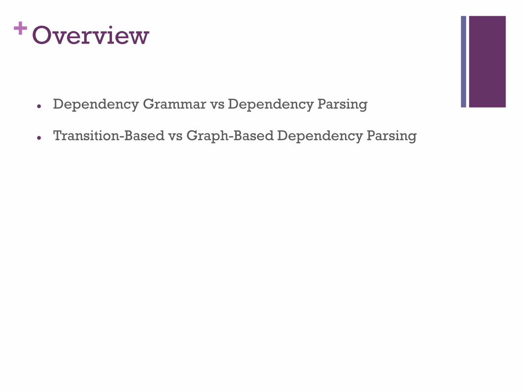
+Syntactic Theories
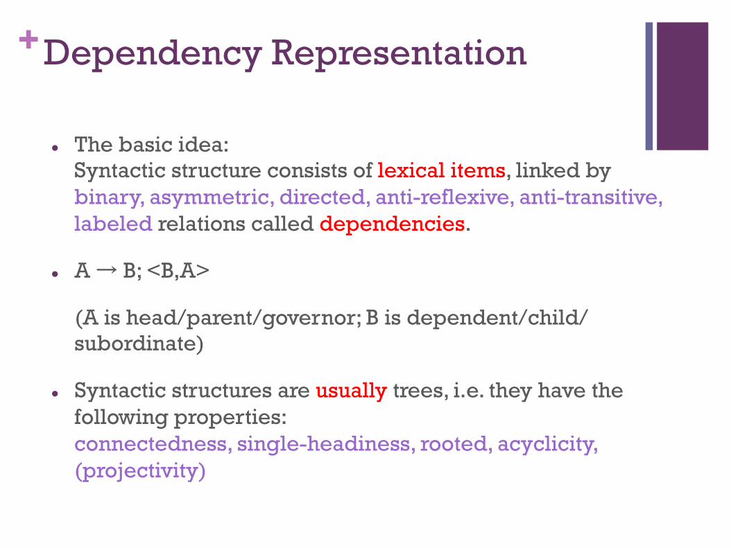
+Dependency Representation
l The basic idea: Syntactic structure consists of lexical items, linked by binary, asymmetric, directed, anti-reflexive, anti-transitive, labeled relations called dependencies.
l A → B; <B,A>
(A is head/parent/governor; B is dependent/child/subordinate)
l Syntactic structures are usually trees, i.e. they have the following properties: connectedness, single-headiness, rooted, acyclicity, (projectivity)
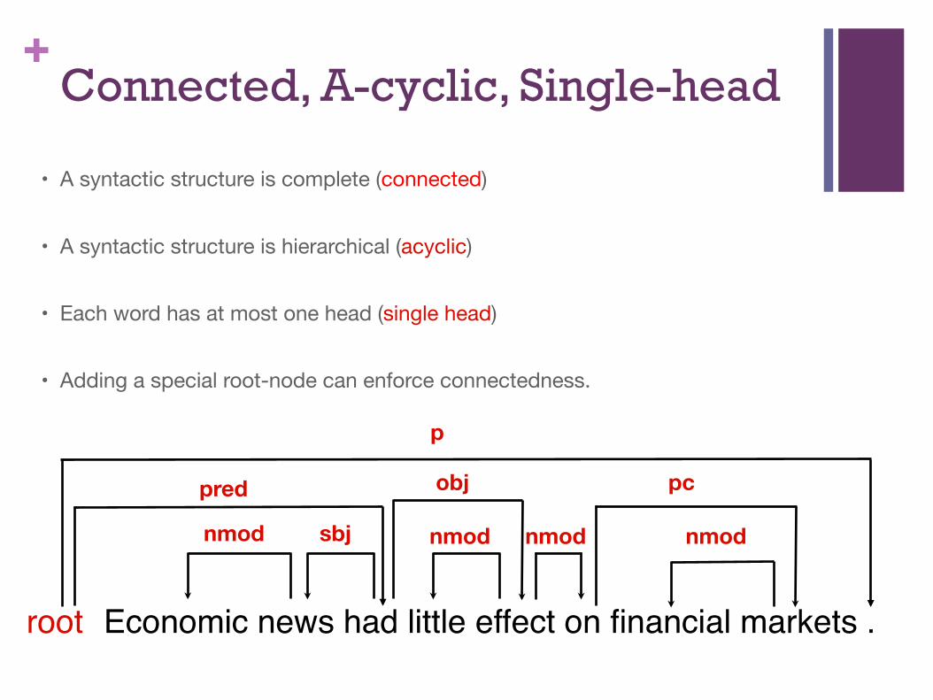
+Connected, A-cyclic, Single-head
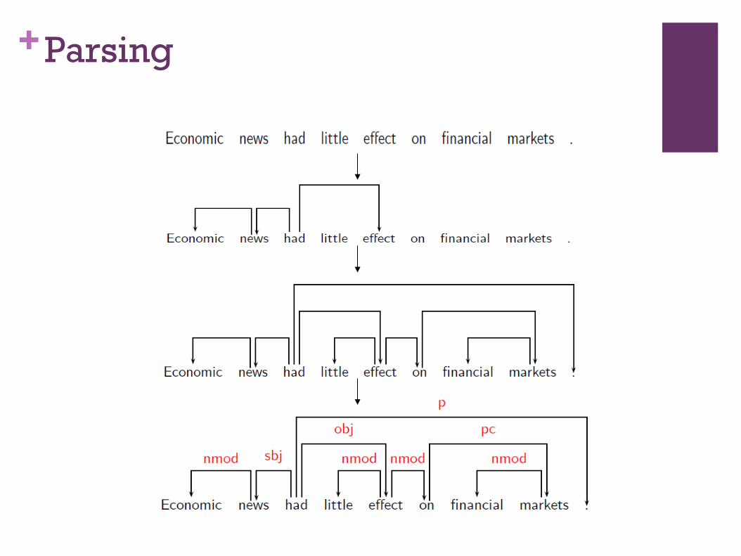
Economic news had little effect on financial markets .
sbj nmod
obj
nmod nmod nmod
pc
root
pred
p
• A syntactic structure is complete (connected)
• A syntactic structure is hierarchical (acyclic)
• Each word has at most one head (single head)
• Adding a special root-node can enforce connectedness.
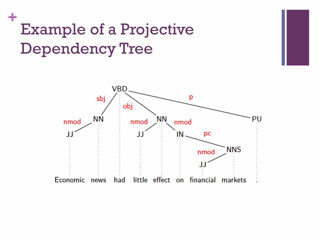
+Example of a Projective Dependency Tree
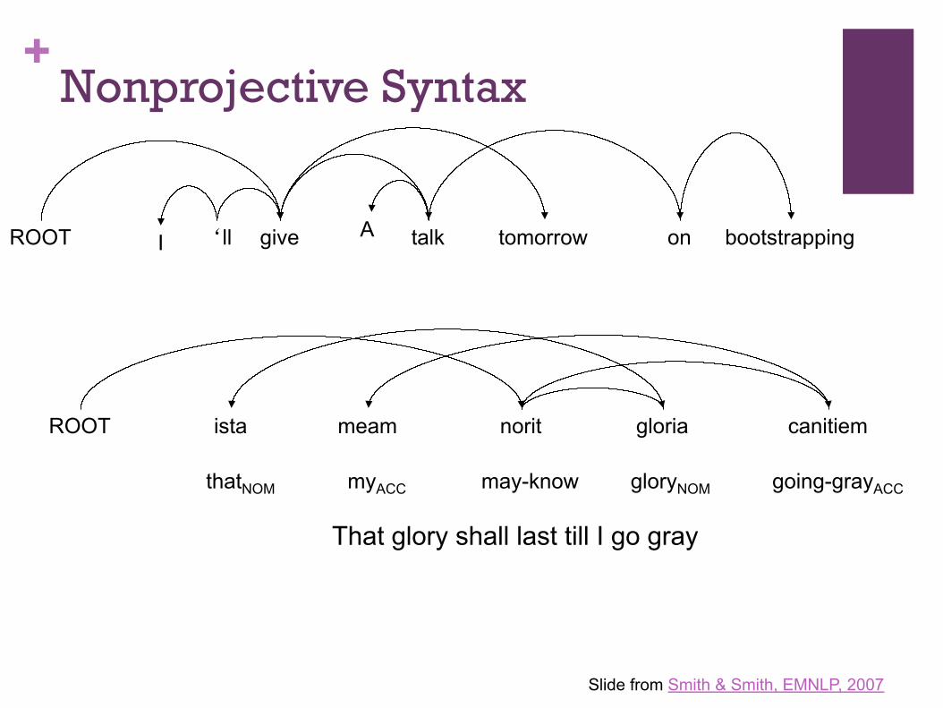
+Nonprojective Syntax
ista meam norit gloria canitiem ROOT
I give A on bootstrapping talk tomorrow ROOT ‘ll
thatNOM myACC may-know gloryNOM going-grayACC
That glory shall last till I go gray
Slide from Smith & Smith, EMNLP, 2007
+Dependency Grammar
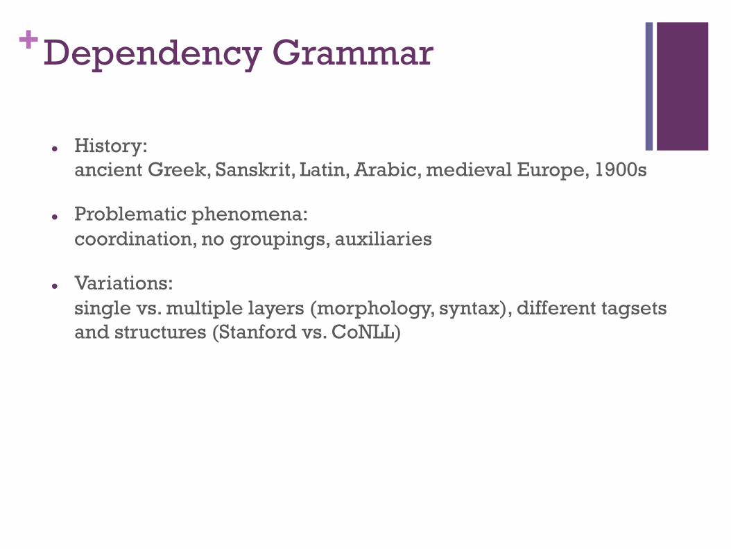
l History: ancient Greek, Sanskrit, Latin, Arabic, medieval Europe, 1900s
l Problematic phenomena: coordination, no groupings, auxiliaries
l Variations: single vs. multiple layers (morphology, syntax), different tagsets and structures (Stanford vs. CoNLL)
+Dependency Parsing
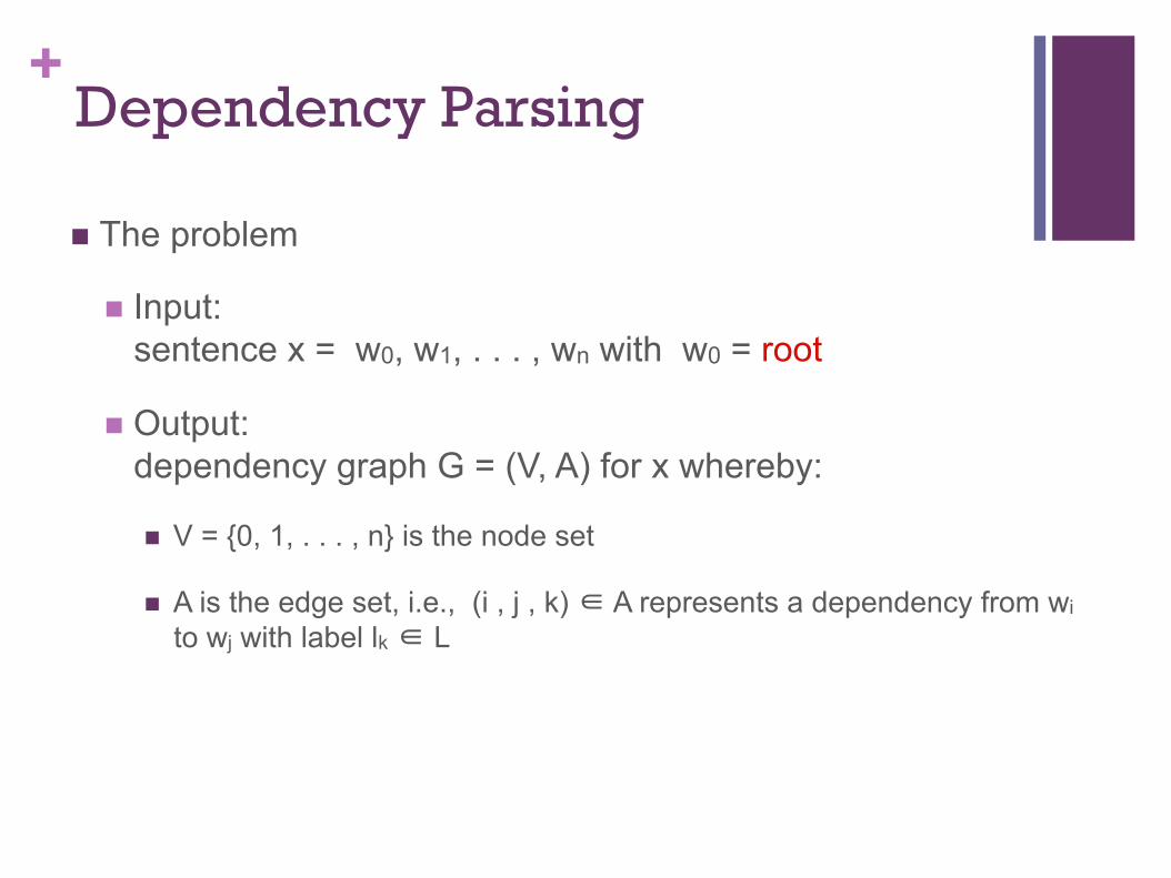
n The problem
n Input: sentence x = w0, w1, . . . , wn with w0 = root
n Output: dependency graph G = (V, A) for x whereby:
n V = {0, 1, . . . , n} is the node set
n A is the edge set, i.e., (i , j , k) ∈ A represents a dependency from wi to wj with label lk ∈ L
+Parsing
+Dependency Parsing
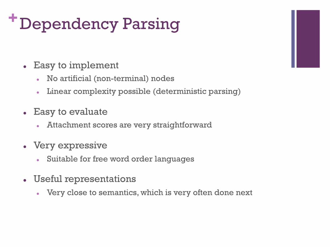
l Easy to implement l No artificial (non-terminal) nodes
l Linear complexity possible (deterministic parsing)
l Easy to evaluate l Attachment scores are very straightforward
l Very expressive l Suitable for free word order languages
l Useful representations l Very close to semantics, which is very often done next
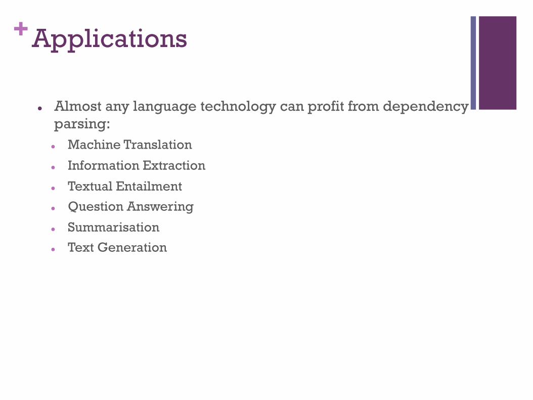
+Applications
l Almost any language technology can profit from dependency parsing:
l Machine Translation
l Information Extraction
l Textual Entailment
l Question Answering
l Summarisation
l Text Generation
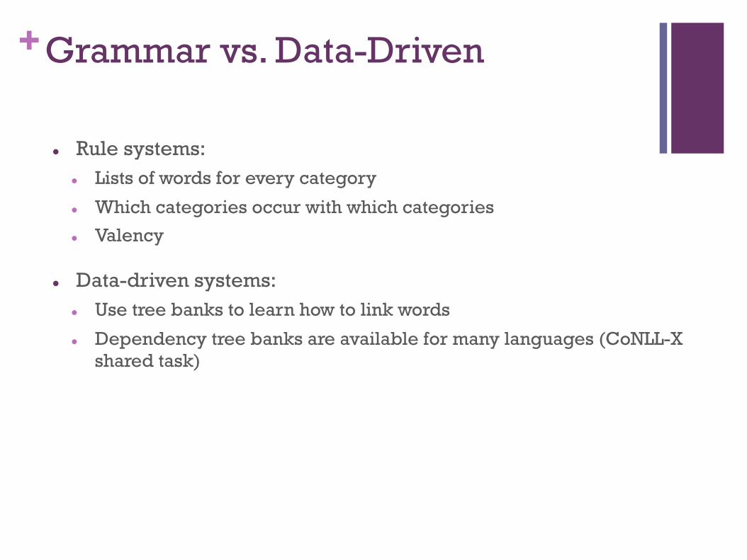
+Grammar vs. Data-Driven
l Rule systems: l Lists of words for every category
l Which categories occur with which categories
l Valency
l Data-driven systems: l Use tree banks to learn how to link words
l Dependency tree banks are available for many languages (CoNLL-X shared task)
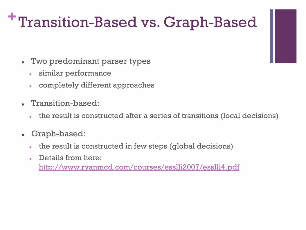
+Transition-Based vs. Graph-Based
l Two predominant parser types l similar performance
l completely different approaches
l Transition-based: l the result is constructed after a series of transitions (local decisions)
l Graph-based: l the result is constructed in few steps (global decisions)
l Details from here: http://www.ryanmcd.com/courses/esslli2007/esslli4.pdf
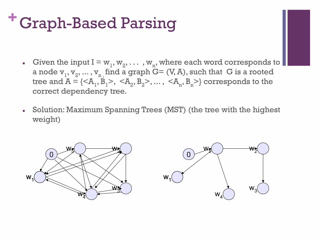
+Graph-Based Parsing
l Given the input I = w1, w2, . . . , wn, where each word corresponds to a node v1, v2, ... , vn , find a graph G= (V, A), such that G is a rooted tree and A = {<A1, B1>, <A2, B2>, ... , <An, Bn>} corresponds to the correct dependency tree.
l Solution: Maximum Spanning Trees (MST) (the tree with the highest weight)
0
w1 w1
w3
w5 w2
w4
0
w1 w1
w3
w5 w2
w4
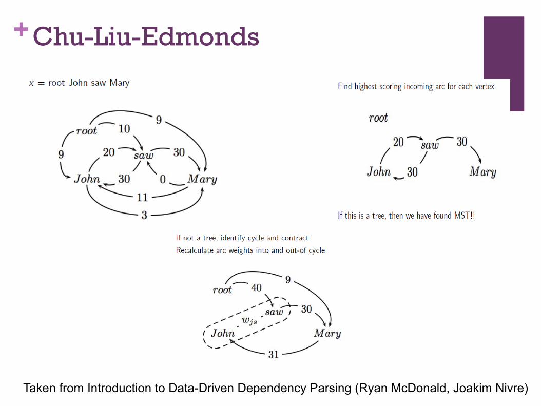
+Chu-Liu-Edmonds
Taken from Introduction to Data-Driven Dependency Parsing (Ryan McDonald, Joakim Nivre)
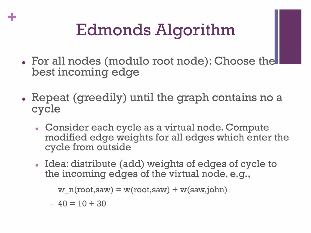
+Edmonds Algorithm
l For all nodes (modulo root node): Choose the best incoming edge
l Repeat (greedily) until the graph contains no a cycle
l Consider each cycle as a virtual node. Compute modified edge weights for all edges which enter the cycle from outside
l Idea: distribute (add) weights of edges of cycle to the incoming edges of the virtual node, e.g.,
- w_n(root,saw) = w(root,saw) + w(saw,john)
- 40 = 10 + 30
+Graph-Based Parsing
l Advantages: l State-of-the art performance
l Works well for long sentences/dependencies
l Disadvantages: l Not incremental
l Computationally expensive (Chu-Liu-Edmonds need O(n*n) to find MST)
+Transition-Based Parsing
l The parse of the sentence is a sequence of operations (transitions)
l The result is a complete set of dependency pairs, which satisfy tree constraints
l An oracle tells the parser what action should be taken in every step:
l Training - use training data for simulating a perfect oracle (you have the desired result given)
l Application - use classifiers for simulating an oracle (train models, that allow the oracle to choose correct actions)
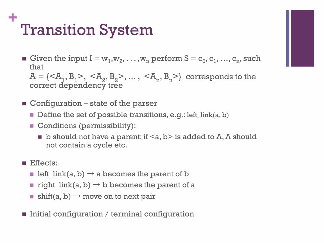
+Transition System
n Given the input I = w1,w2, . . . ,wn perform S = c0, c1, …, cn, such that A = {<A1, B1>, <A2, B2>, ... , <An, Bn>} corresponds to the correct dependency tree
n Configuration – state of the parser n Define the set of possible transitions, e.g.: left_link(a, b) n Conditions (permissibility):
n b should not have a parent; if <a, b> is added to A, A should not contain a cycle etc.
n Effects: n left_link(a, b) → a becomes the parent of b n right_link(a, b) → b becomes the parent of a n shift(a, b) → move on to next pair
n Initial configuration / terminal configuration
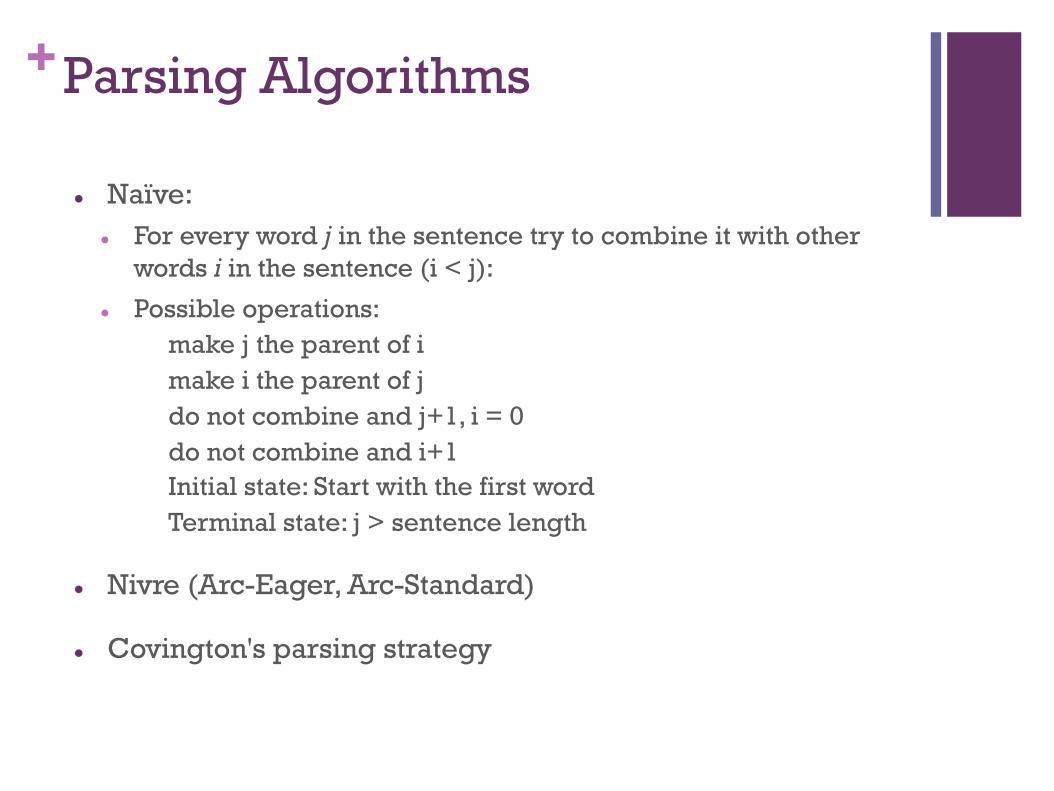
+Parsing Algorithms
l Naïve: l For every word j in the sentence try to combine it with other
words i in the sentence (i < j):
l Possible operations: make j the parent of i make i the parent of j do not combine and j+1, i = 0 do not combine and i+1 Initial state: Start with the first word Terminal state: j > sentence length
l Nivre (Arc-Eager, Arc-Standard)
l Covington's parsing strategy
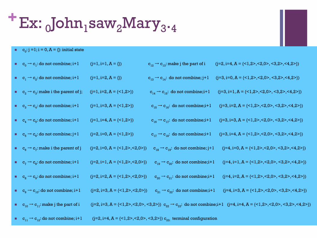
+Ex: 0John1saw2Mary3.4
n c0: j =1; i = 0, A = {}: initial state
n c0 → c1: do not combine; i+1 (j=1, i=1, A = {}) c12 → c13: make j the part of i (j=2, i=4, A = {<1,2>,<2,0>, <3,2>,<4,2>})
n c1 → c2: do not combine; i+1 (j=1, i=2, A = {}) c13 → c14: do not combine; j+1 (j=3, i=0, A = {<1,2>,<2,0>, <3,2>,<4,2>})
n c2 → c3: make i the parent of j; (j=1, i=2, A = {<1,2>}) c14 → c15: do not combine;i+1 (j=3, i=1, A = {<1,2>,<2,0>, <3,2>,<4,2>})
n c3 → c4: do not combine; i+1 (j=1, i=3, A = {<1,2>}) c15 → c16: do not combine;i+1 (j=3, i=2, A = {<1,2>,<2,0>, <3,2>,<4,2>})
n c4 → c5: do not combine; i+1 (j=1, i=4, A = {<1,2>}) c16 → c17: do not combine;i+1 (j=3, i=3, A = {<1,2>,<2,0>, <3,2>,<4,2>})
n c5 → c6: do not combine; j+1 (j=2, i=0, A = {<1,2>}) c17 → c18: do not combine;i+1 (j=3, i=4, A = {<1,2>,<2,0>, <3,2>,<4,2>})
n c6 → c7: make i the parent of j (j=2, i=0, A = {<1,2>,<2,0>}) c18 → c19: do not combine; j+1 (j=4, i=0, A = {<1,2>,<2,0>, <3,2>,<4,2>})
n c7 → c8: do not combine; i+1 (j=2, i=1, A = {<1,2>,<2,0>}) c19 → c20: do not combine;i+1 (j=4, i=1, A = {<1,2>,<2,0>, <3,2>,<4,2>})
n c8 → c9: do not combine; i+1 (j=2, i=2, A = {<1,2>,<2,0>}) c20 → c21: do not combine;i+1 (j=4, i=2, A = {<1,2>,<2,0>, <3,2>,<4,2>})
n c9 → c10: do not combine; i+1 (j=2, i=3, A = {<1,2>,<2,0>}) c21 → c22: do not combine;i+1 (j=4, i=3, A = {<1,2>,<2,0>, <3,2>,<4,2>})
n c10 → c11: make j the part of i (j=2, i=3, A = {<1,2>,<2,0>, <3,2>}) c22 → c23: do not combine;i+1 (j=4, i=4, A = {<1,2>,<2,0>, <3,2>,<4,2>})
n c11 → c12: do not combine; i+1 (j=2, i=4, A = {<1,2>,<2,0>, <3,2>}) c23: terminal configuration
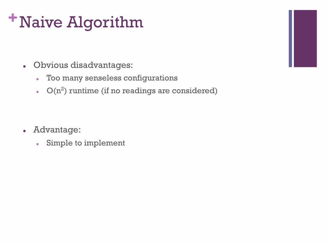
+Naive Algorithm
l Obvious disadvantages: l Too many senseless configurations
l O(n2) runtime (if no readings are considered)
l Advantage: l Simple to implement
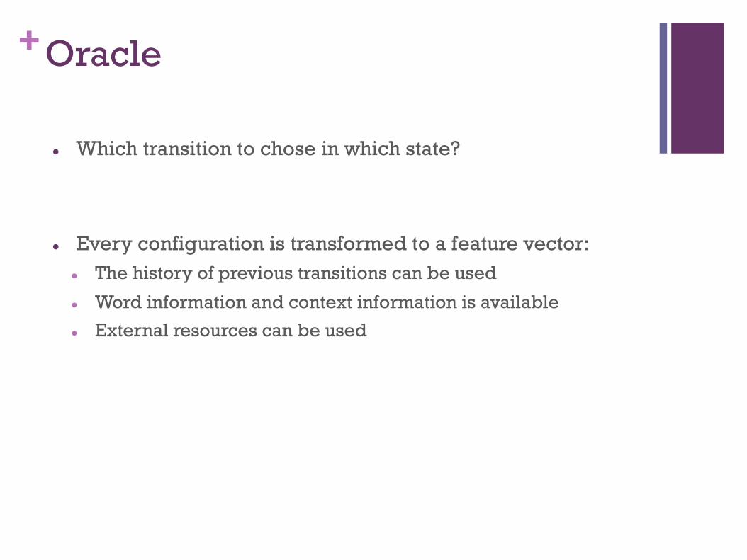
+Oracle
l Which transition to chose in which state?
l Every configuration is transformed to a feature vector: l The history of previous transitions can be used
l Word information and context information is available
l External resources can be used
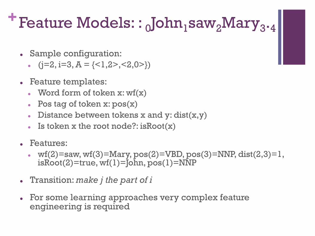
+Feature Models: : 0John1saw2Mary3.4 l Sample configuration:
l (j=2, i=3, A = {<1,2>,<2,0>})
l Feature templates: l Word form of token x: wf(x) l Pos tag of token x: pos(x) l Distance between tokens x and y: dist(x,y) l Is token x the root node?: isRoot(x)
l Features: l wf(2)=saw, wf(3)=Mary, pos(2)=VBD, pos(3)=NNP, dist(2,3)=1,
isRoot(2)=true, wf(1)=John, pos(1)=NNP
l Transition: make j the part of i
l For some learning approaches very complex feature engineering is required
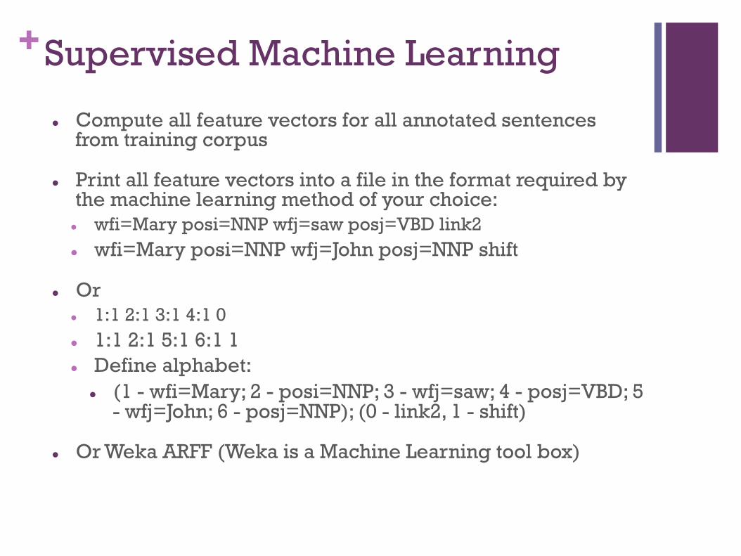
+Supervised Machine Learning
l Compute all feature vectors for all annotated sentences from training corpus
l Print all feature vectors into a file in the format required by the machine learning method of your choice:
l wfi=Mary posi=NNP wfj=saw posj=VBD link2 l wfi=Mary posi=NNP wfj=John posj=NNP shift
l Or l 1:1 2:1 3:1 4:1 0 l 1:1 2:1 5:1 6:1 1 l Define alphabet:
l (1 - wfi=Mary; 2 - posi=NNP; 3 - wfj=saw; 4 - posj=VBD; 5 - wfj=John; 6 - posj=NNP); (0 - link2, 1 - shift)
l Or Weka ARFF (Weka is a Machine Learning tool box)
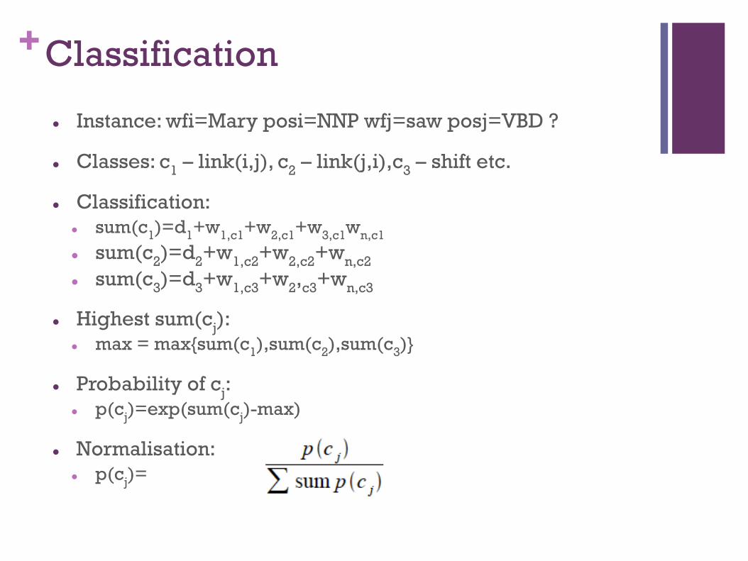
+Classification
l Instance: wfi=Mary posi=NNP wfj=saw posj=VBD ?
l Classes: c1 – link(i,j), c2 – link(j,i),c3 – shift etc.
l Classification: l sum(c1)=d1+w1,c1+w2,c1+w3,c1wn,c1
l sum(c2)=d2+w1,c2+w2,c2+wn,c2 l sum(c3)=d3+w1,c3+w2,c3+wn,c3
l Highest sum(cj): l max = max{sum(c1),sum(c2),sum(c3)}
l Probability of cj: l p(cj)=exp(sum(cj)-max)
l Normalisation: l p(cj)=
+Classification
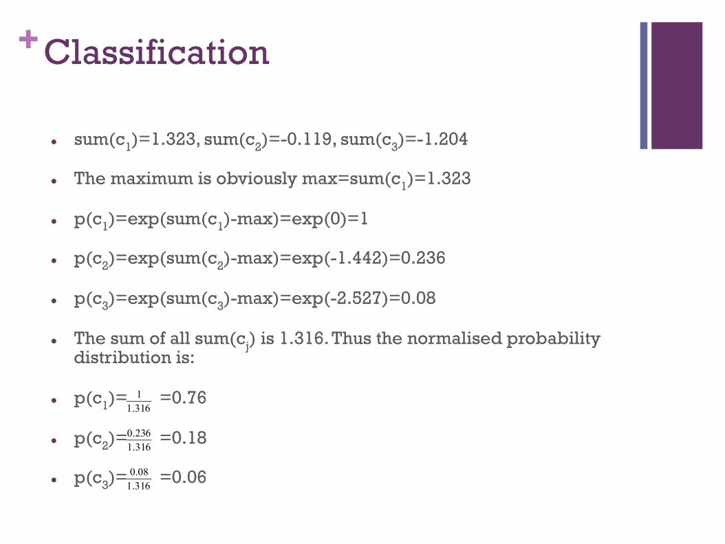
l sum(c1)=1.323, sum(c2)=-0.119, sum(c3)=-1.204
l The maximum is obviously max=sum(c1)=1.323
l p(c1)=exp(sum(c1)-max)=exp(0)=1
l p(c2)=exp(sum(c2)-max)=exp(-1.442)=0.236
l p(c3)=exp(sum(c3)-max)=exp(-2.527)=0.08
l The sum of all sum(cj) is 1.316. Thus the normalised probability distribution is:
l p(c1)= =0.76
l p(c2)= =0.18
l p(c3)= =0.06
11.316
0.2361.316
0.081.316
+Summary
l Dependency Grammar and Parsing
l Graph-based parsing
l Transition-based approach
l Learning and Classification