Embed Size (px)
Citation preview

Dependence in non-life insurance
Hanna Arvidsson and Sofie Francke
U.U.D.M. Project Report 2007:23
Examensarbete i matematisk statistik, 20 poäng
Handledare och examinator: Ingemar Kaj
Juni 2007
Department of Mathematics
Uppsala University


Dependence in non-life insurance
Hanna Arvidsson and Sofie Francke
June 2007
Abstract In insurance mathematics independence is usually assumed be-tween all variables. In this paper we describe a few ways of modeling de-pendency in non-life insurance. We look especially close at a model calledthe Compound Markov Binomial Model that models a dependency betweenclaim occurrences. We also examine if this kind of dependency exists in datafrom Folksam’s ”allrisk”-insurance.
1

Acknowledgements We want to thank our supervisor, Ingemar Kaj, forall the help and guidance along the way and for always being available. Wewould also like to thank Robert Nygren at Folksam for providing us with datamaterial and answering our questions. Finally we thank Silvelyn Zwanzig forthe help with the likelihood ratio test and Christian Baath for the assistancewith transferring the data material into Matlab friendly format.
2

Contents
1 Introduction 5
1.1 Basic insurance mathematics . . . . . . . . . . . . . . . . . . . 51.2 Basic Markov theory . . . . . . . . . . . . . . . . . . . . . . . 6
2 A model with dependency between classes of business and
groups of events 7
3 Modeling dependency with Copulas 9
3.1 The Normal Copula Model . . . . . . . . . . . . . . . . . . . . 93.1.1 Simulation of the Normal Copula Model . . . . . . . . 10
4 A model with dependence between claim sizes and claim in-
tervals 12
4.1 Model 1 . . . . . . . . . . . . . . . . . . . . . . . . . . . . . . 124.1.1 A variant of Model 1 . . . . . . . . . . . . . . . . . . . 13
4.2 Model 2 . . . . . . . . . . . . . . . . . . . . . . . . . . . . . . 134.3 Survival probabilities for Model 1 . . . . . . . . . . . . . . . . 13
5 The Compound Markov Binomial Model 16
5.1 Introduction . . . . . . . . . . . . . . . . . . . . . . . . . . . . 165.2 The Markov Bernoulli Model . . . . . . . . . . . . . . . . . . . 175.3 The Markov Binomial Model . . . . . . . . . . . . . . . . . . . 195.4 The Compound Markov Binomial Model . . . . . . . . . . . . 22
5.4.1 Survival probabilities . . . . . . . . . . . . . . . . . . . 245.5 Estimating survival probabilities by simulation . . . . . . . . . 26
5.5.1 Simulation . . . . . . . . . . . . . . . . . . . . . . . . . 26
6 Maximum likelihood estimations and likelihood ratio test 28
6.1 Maximum likelihood estimations for the variables in the com-pound Markov binomial model . . . . . . . . . . . . . . . . . . 286.1.1 Confidence intervals . . . . . . . . . . . . . . . . . . . 31
6.2 Likelihood ratio test using the bootstrap method . . . . . . . 32
7 Fitting data to the compound Markov binomial model 34
7.1 Claims . . . . . . . . . . . . . . . . . . . . . . . . . . . . . . . 357.2 Estimations . . . . . . . . . . . . . . . . . . . . . . . . . . . . 39
7.2.1 The maximum likelihood estimations . . . . . . . . . . 407.2.2 Likelihood ratio test . . . . . . . . . . . . . . . . . . . 447.2.3 Confidence intervals . . . . . . . . . . . . . . . . . . . 467.2.4 Stationarity . . . . . . . . . . . . . . . . . . . . . . . . 47
3

7.2.5 Probability of survival . . . . . . . . . . . . . . . . . . 47
8 Discussion 49
4

1 Introduction
This paper will describe four different ways of modeling dependence in non-life insurance. The first three models will only be covered by a summary whilethe focus of the paper will be on the fourth model, the compound Markovbinomial model, for which there will also be some numerical estimations.
Sections 1.1 and 1.2 contain a short introduction to non-life insurancemathematics and Markov theory needed to understand the following sections.In section 2 a model with dependence between classes of business and groupsof events is presented. This is followed by a model which uses copulas todescribe a dependence between claim sizes in section 3 and a model withdependence between claim sizes and claim intervals in section 4.
The main part of the paper starts in section 5 where the compoundMarkov binomial model, which models dependency between claim occur-rences, is described in detail. This is is followed by methods for estimatingthe parameters in the model and testing these estimations, which are thenused on data from Folksam’s ”allrisk”-insurance in section 7.
1.1 Basic insurance mathematics
The collective claim size in an insurance portfolio is usually described by themodel
S(t) =
N(t)∑
i=1
Xi, (1)
where S(t) is the claim size up to time t, Xi is the size of claim i and N(t)is the number of claims up until time t. Normally the Xi:s are assumed tobe independent, identically distributed (i.i.d.) random variables and inde-pendent of N(t). The surplus, R(t), of the portfolio at time t is describedby
R(t) = x+ ct− S(t), (2)
where x is the initial capital and c is the premium density.When looking at the probability of ruin of an insurance portfolio we start
by defining the random variable T, which is the time of ruin, as follows
T =
inf {t > 0 : R(t) < 0} if R(t) falls below 0 at least once
∞ else
5
The probability of ruin before time t with initial capital x, denoted ψ(x, t),is then
ψ(x, t) = Pr(T < t). (3)
Of primary interest is the probability of ever reaching ruin with initial capitalx, denoted ψ(x), that is
ψ(x) = Pr(T <∞). (4)
It is often more natural to consider the probability that the portfolio willcarry its cost, therefore the finite and infinite probabilities of non-ruin areused, which are denoted
φ(x, t) = 1 − ψ(x, t) (5)
andφ(x) = 1 − ψ(x). (6)
1.2 Basic Markov theory
In this paper only discrete Markov processes with discrete state spaces will beconsidered, these are often called discrete Markov chains. This means thatif {Xn}
∞
n=0 is a time discrete stochastic process with non-negative integerstates, then for each n > 0 and every event in i0, i1, . . . , in+1 it holds that
Pr (Xn+1 = in+1 | Xn = in, Xn−1 = in−1, . . . , X0 = i0)
= Pr (Xn+1 = in+1 | Xn) .
This equation is also known as the Markov Property. The transition proba-bilities will be defined by
pij = Pr(Xn+1 = j|Xn = i).
The models used in this paper require that the Markov chain is stationarywhich means that the probability Pr(Xn = i) is independent of n for all i inthe state space. In our case this will mean that the probability of a claim,not conditioned on the previous period, will be the same for all time periods.
6
2 A model with dependency between classes
of business and groups of events
In [Wang and Yuen, 2005] the dependence between different classes of busi-ness is examined. An example of how a claim in one class of insurance caninduce a claim in a different class mentioned in this work is car accidents.The damaged cars will lead to claims in one insurance class while personalinjuries will lead to claims in a different class. Suppose that an insurancecompany has n (n > 1) dependent classes of business. The stochastic eventsare divided into m groups and each event is assumed to be able to cause aclaim in at least one of the classes. In the example the stochastic event is thecar accident. Each claim in the k’th group of stochastic events may causea claim in the j’th class at time t with probability pkj(t) for k = 1, 2, . . . , mand j = 1, 2, . . . , n. For each j there exists at least one k such that pkj(t) > 0which means that for each class there is at least one group with a non-zeroprobability for a claim in that class. The number of claims caused by eventsin the k’th group up until time t is denoted Nk(t) and Nk
j (t) is the numberof claims from the k’th group in the j’th class up until time t. The claimamount of the i’th claim in the j’th class will be denoted X j
i . This leads tothe following expression for the total amount of claims for the j’th class ofbusiness up until time t
Sj(t) =
Nj(t)∑
i=1
X(j)i .
From this expression the total amount of claims up until time t for all classescan be obtained
S(t) =
n∑
j=1
Sj(t) =
n∑
j=1
Nj(t)∑
i=1
X(j)i
where {X(j)i : i = 1, 2, . . .} is assumed to be a sequence of i.i.d. non-negative
random variables with common distribution function Fj for each j. The n
sequences {X(j)i : i = 1, 2, . . .}, . . . , {X
(n)i : i = 1, 2, . . .} are assumed to
be independent of each other and also independent of the claim numberprocesses. The surplus is defined as
R(t) = x + ct− S(t) = x + ct−n∑
j=1
Sj(t) = x+ ct−n∑
j=1
Nj(t)∑
i=1
X(j)i
7

The following assumptions are needed to analyze R(t).
1) The processes N 1(t), N2(t), . . . , Nm(t) are independent Poisson processeswith parameters λ1, λ2, . . . , λm respectively. The two vectors of claim num-ber processes, (Nk(t), Nk
1 (t), . . . , Nkn(t)) and (Nk′
(t), Nk′
1 (t), . . . , Nk′
n (t)), areindependent for k 6= k′.
2) Given Nk(t), the claim number processes, Nk1 (t), . . . , Nk
n(t), are condi-tionally independent for each k, k = 1, 2, . . . , m.
In [Wang and Yuen, 2005] upper bounds for the ruin probability, definedas ψ(x) = Pr(inft≥0R(t) < 0), of the portfolio are derived using martin-gales and the Lundberg exponent. The influence of the dependency betweenthe claim number processes on the ruin probability is also examined. Theclassification of the stochastic events and the effect of misclassification onthe surplus process are studied. There is also a numerical example with aprocess with 2 groups and 2 classes. In the example the ruin probabilityfor the simplified model with two groups is compared to the ruin probabilitywhen the process is misclassified with only 1 group and to the calculated ruinprobability when independence is assumed. The conclusion of the example isthat the misclassified model overestimates the probability of ruin while theindependent model underestimates it which shows that the classifications ofthe stochastic events are important in this model.
8

3 Modeling dependency with Copulas
In [Albrecher, 1998] a model is described for dependency between claim sizesby using copulas. This model is suggested for large claims, for exampleextreme natural events. In [Klaassen and Wellner, 1997] a copula is describedas a distribution function on the unit cube [0, 1]m with uniform marginaldistributions. Suppose that we have two random variables, X and Y , withdistribution functions F (x) and G (y) respectively. Then for each x and y,F (x) and G (y) are represented by a real number each in the interval [0, 1].These numbers are mapped by the copula to the joint distribution function.Here the normal copula will be used to model the dependency between theclaim sizes. This will be followed by an explanation on how to simulatethe ruin probabilities using copulas and the Monte Carlo method used in[Albrecher, 1998].
In this paper only copulas that join two random variables will be used.For copulas of higher dimensions see [Nelsen, 2006].
Sklar’s Theorem (See e.g. [Nelsen, 2006]) Let X and Y be two randomvariables with joint distribution function H and marginal distribution func-tions F and G, respectively. Then there exists a copula, C(u, v), such thatfor all x, y in (−∞,+∞)
H (x, y) = C (F (x) , G (y)) . (7)
If F and G are continuous the copula is unique and otherwise it is uniquelydetermined on RanF × RanG. The equation can also be used to determinethe joint distribution function when the copula is known.
3.1 The Normal Copula Model
In [Albrecher, 1998] the claim sizes, {X1, X2, . . .}, are assumed to be i.i.d.positive random variables with distribution function F and finite mean µ =E(X1). The k’th claim arrives at time Tk = D1+D2+. . .+Dk, according to ahomogeneous Poisson process, where the time between claims, {D1, D2, . . .}are i.i.d. exponentially distributed random variables with intensity α. Inthis model the goal is to combine an independent random variable with theprevious claim size to get the next claim size. This is only possible to dowith the normal copula. According to [Nelsen, 2006] Sklar’s theorem for aNormal copula results in the following expression.
C (u, v; ρ) = ΦΣ(ρ)
(Φ−1 (u) ,Φ−1 (v)
)(8)
9

where
Σ (ρ) =
(1 ρρ 1
), −1 ≤ ρ ≤ 1,
ΦΣ(ρ) is the bivariate normal distribution with mean vector zero and covari-ance matrix Σ (ρ) and u, v are uniformly distributed. In the Normal CopulaModel it is assumed that Yi = Xi − cDi, where Xi is the i’th claim, c is thepremium rate and Di is the time between the (i− 1)’th and the i’th claim.This means that you would want a c that gives a negative expected value forYi.
Suppose that {Y1, Z2, Z3, . . .} are i.i.d. with distribution function F . ThenSklar’s theorem together with the fact that the distribution function of arandom variable itself is uniformly distributed on the interval [0, 1] results in
F (Yi+1) = C (F (Yi) , F (Zi+1))
which leads to
F (Yi+1) = ΦΣ(ρ)
(Φ−1 (F (Yi)) ,Φ
−1 (F (Zi+1)))
= Φ(ρΦ−1 (F (Yi)) +
√1 − ρ2Φ−1 (F (Zi+1))
) (9)
By inverting both sides
Yi+1 = F−1[Φ
(ρΦ−1 (F (Yi)) +
√1 − ρ2Φ−1 (F (Zi+1))
)](10)
is obtained. This means that the (i+ 1)′ th claim size is dependent on thei’th claim size and a random variable Zi+1, which are joined through a normalcopula. In (10), ρ = 1 would result in complete dependence, while ρ = 0would mean that Yi+1 is independent of Yi.
3.1.1 Simulation of the Normal Copula Model
In [Albrecher, 1998] a Monte Carlo method is used to simulate the Normalcopula model. A simulation is made for {Y1, Z2, Z3, . . .} for some distribution.In [Albrecher, 1998] the distribution function of X, F , is assumed to beexponential. Then {Y2, Y3, . . . , Yk} are computed by using (10) and Y1 +Y2 +. . .+ Yk constitute one trajectory in k steps. N trajectories are simulated inthe same way and the percentage of trajectories leading to ruin are calculatedby using the formula
ψ =1
N
∑
Zt∈Z
1A (zt) ,
where Z is the set of all N trajectories and A is the set of trajectories leadingto ruin. To get a reasonable variance for the result of this Monte Carlo
10

method a very large number of trajectories would be needed. In order tokeep the variance down importance sampling is used. This method increasesthe chances of ruin and therefore reduces the variance of the estimated value.Suppose that f is the density function of each step Yi, and g is a densityfunction chosen in such a way that using g would lead to considerably moretrajectories leading to ruin than using f . Then
P (zt ∈ A) = Ef (1A (zt)) =
∫1A (zt) f (x) dx
=
∫1A (zt)
f (x)
g (x)g (x) dx = E
(1A (zt)
f (zt)
g (zt)
).
This leads to
ψ =1
N
∑
Z
P (zt ∈ A) =1
N
∑
Z
E
(1A (zt)
f (zt)
g (zt)
).
So the equation used to estimate the ruin probability will be
ψ =1
N
∑
Z
1A (zt)
∏
i
f (zti)
∏
i
g (zti). (11)
In [Albrecher, 1998] a simulation is done for different values of ρ and x.It is concluded that with an increasing ρ the ruin probability also increases,while it decreases with an increasing x. A sensitivity result is also proposedfor the trajectory on the boundary between the independent and the de-pendent case. The sensitivity result shows that extreme events increase thederivative for later events and therefore they can increase the probability ofruin.
11

4 A model with dependence between claim
sizes and claim intervals
In this continuous model, proposed in [Albrecher and Boxma, 2004] the ideais to allow a dependency between the size of claim i and the inter-occurrencetime between claim i and claim i + 1. The surplus process R(t) for theinsurance portfolio is, as described before,
R(t) = x + ct−
N(t)∑
i=1
Xi, (12)
where x is the initial capital, c is the premium which is assumed to be aconstant, Xi is the size of claim i and N(t) is the number of claims upuntil time t. The Xi:s are i.i.d. random variables with distribution functionF (.). In [Albrecher and Boxma, 2004] two related models are presented, plusa variant of the first model. For all the models Albrecher and Boxma useLaplace-Stieltje transforms to derive expressions for the Laplace transformof the probability of survival, which they also show can be used to calculatethe probability of survival of the process explicitly if the claims have a phase-type distribution. This makes it possible to make numerical examples wherethe dependent case can be compared with the independent case to see howthe dependency affects the probability of survival. Phase-type distributionsinclude the exponential and gamma distributions. In this text the two modelswill be described, but the formulas needed to derive the survival probabilitywill only be shown for Model 1 to exemplify in what form the formulas arepresented. The expressions for the other models are similar.
4.1 Model 1
If a claim, Xi, is larger than a threshold, Ti, the time until the next claim,Wi+1, is exponentially distributed with rate λ1, if not it is exponentiallydistributed with rate λ2. The thresholds are i.i.d. random variables withdistribution function T (.). The net profit condition for the model is
E(X) < c
[P (X > T )
λ1+P (X ≤ T )
λ2
]. (13)
If this condition does not hold the probability of ruin will be 1.Depending on how λ1 and λ2 are chosen, and which kind of thresholds areused, the model can apply to quite different scenarios. There are three nu-merical examples in [Albrecher and Boxma, 2004], in which X and T have
12

exponential distributions. In the first one λ1 > λ2, meaning that a largeclaim is more likely to be followed by a short inter-occurrence time. Forthis example Albrecher and Boxma compare the ruin probability of the de-pendent model with the ruin probability when independence is assumed andshow that the independent model overestimates the survival probability. Inthe second example λ1 < λ2, and in this case the independent model underes-timated the survival probability. In the last example the survival probabilityof the dependent model with T ∈ Exp(1) is compared with the survival prob-ability of the same model but with T = 1, and it is shown that the choice ofthresholds has a significant effect on the survival probability.
4.1.1 A variant of Model 1
The inter-occurrence time, Wi+1, is still Exp(1/λ1)-distributed if Xi > Ti andExp(1/λ2)-distributed ifXi ≤ Ti for all i ≥ 1, but the reimbursement that theinsurance company pays for the claim is now min(Xi, Ti). This represents thecase when the insurance company has a ceiling for the reimbursement of eachclaim or when they have a reinsurance of XL-type. An XL-type reinsurance iswhen the insurance company, Company A, insures itself against claims largerthan a threshold, Ti, by signing a reinsurance with a reinsurance company,Company B, where it is agreed that Company B will reimburse Company Awith Xi − Ti for claims exceeding the thresholds.
4.2 Model 2
For every t > 0 the process is said to be in one of two states, i = 1, 2, whichcorresponds to the intensity λi of the exponential distribution for the inter-occurrence time. In this model the process changes state when a claim occursif the claim size Xi is smaller than the threshold Ti, otherwise the processwill remain in the current state. The net profit condition for this model is
2E(X) < c
(1
λ1+
1
λ2
).
4.3 Survival probabilities for Model 1
To calculate the probability of survival,
φ(x) = Pr(R(t) ≥ 0 ∀t > 0 | R(0) = x),
the net profit condition and Pr(X > 0) = P (T > 0) = 1 are assumed tobe fulfilled. When the time until the first claim is exponentially distributed
13
with intensity λi, the probability of survival with initial capital x is denotedby φi(x), (i = 1, 2). The survival probability is first described as
φi(x) = (1 − λidt)︸ ︷︷ ︸Pr(no claim in [0, dt])
×φi(x + cdt) + λidt︸︷︷︸Pr(a claim in [0, dt])
×
∫ x+cdt
0
[Pr(T ≤ y)φ1(x+ cdt− y) + Pr(T > y)φ2(x + cdt− y)]dF (y)
(14)
If there is no claim in [0, dt] the survival probability at time dt is φi(x+ cdt)since the exponential distribution has no memory. If there is a claim of sizey at time dt the survival probability is φ2(x + cdt − y) if the threshold T islarger than y and φ1(x+cdt−y) otherwise. By starting in (14) and using the
Laplace-transform φi(s) :=∫ ∞
0e−sxφ1(x)dx, Albrecher and Boxma derive
φ1(s) =cφ1(0+)[cs− λ2 + λ2χ2(s)] − cλ1χ2(s)φ2(0+)
[cs− λ1 + λ1χ1(s)][cs− λ2 + λ2χ2(s)] − λ1λ2χ1(s)χ2(s)(15)
and
φ2(s) =cφ2(0+)[cs− λ1 + λ1χ1(s)] − cλ2χ1(s)φ1(0+)
[cs− λ1 + λ1χ1(s)][cs− λ2 + λ2χ2(s)] − λ1λ2χ1(s)χ2(s)(16)
where
χ1(s) := E(e−sXI(X>T )) =
∫ ∞
x=0
e−sxT (x)dF (x)
χ2(s) := E(e−sXI(X)) =
∫ ∞
x=0
e−sx(1 − T (x))dF (x)
for Re s ≥ 0. To be able to use φ1(x) and φ1(x) for finding the survivalprobabilities, the equations
(1 − φ1(0+))Pr(X > T )
λ1+ (1 − φ2(0+))
Pr(X ≤ T )
λ2=β
c(17)
and
φ2(0+) =cσ − λ2 + λ2χ2(σ)
λ1χ2(σ)φ1(0+) =
λ2χ1(σ)
cσ − λ1 + λ1χ1(σ)φ1(0+) (18)
for determining φ1(0+) and φ2(0+) were derived, where σ in (18) is theunique solution, s, with Re s > 0 of
(cs− λ1 + λ1χ1(s))(cs− λ2 + λ2χ2(s)) − λ1λ2χ1(s)χ2(s) = 0
14

The Laplace-transforms (15) and (16) can be explicitly inverted to find exactformulas for φi(x), i = {1, 2} when χi(s), i = {1, 2} are rational functions,which is fulfilled ifX and T have phase-type distributions. The unconditionalsurvival probability, φ(x), can then be calculated by
φ(x) = Pr(B > T )φ1(x) + Pr(B ≤ T )φ2(x).
15

5 The Compound Markov Binomial Model
5.1 Introduction
The compound Markov binomial model, proposed in [Cossette et al., 2003], isan extension of the compound binomial model, see [Willmot, 1993], and usesMarkov theory to allow a dependency between claim occurrences. This is amodel in discrete time and in every time step a claim occurs with probabilityq. In this section the model will be introduced under the assumption ofindependence between claim occurrences. The dependency and its effectswill be described in the following sections. The individual claim sizes, {Xj :j = 1, 2, . . .}, are a sequence of i.i.d. positive discrete random variables. Theprobability mass function for Xj (j = 1, 2, . . .) is denoted by Pr (X = i) =f (i) . The number of claims in k periods, denoted Mk, is defined by
Mk = I1 + I2 + ... + Ik
where the sequence {Ii : i = 0, 1, 2, . . .} consists of identically distributedBernoulli variables with mean q ∈ (0, 1). If the claim occurrences are assumedto be independent, Mk is a sum of i.i.d. Bernoulli random variables, makingit a binomial random variable. The total claim amount over k periods, Sk,is defined by
Sk =
∑Mk
j=1Xj , Mk > 0
0 , Mk = 0
The initial capital is x and the premium is 1 unit per period, which makesthe surplus
Rk = x+ k − Sk.
How the probability of survival in finite time
φ(x, n) = Pr(Rk ≥ 0 : 0 ≤ k ≤ n)
and in infinite timeφ(x) = Pr(Rk ≥ 0 : k ≥ 0)
are affected by the dependency is of course of great interest. The parametersin the model are assumed to fulfill the condition
qE [X] < 1
where the left side is the expected cost for one time period and the rightside is the premium paid each period. This condition, called the net profitcondition, ensures that
Rka.s.→ ∞ as k → ∞
16

which equivalently means that the infinite-time ruin probability, ψ(x), almostsurely goes to 0 when the initial capital, x, goes to infinity. For a definitionof the term almost surely see [Gut, 1995].
The next section will describe how the dependency between the claimoccurrences are modeled. Sections 5.3 and 5.4 will cover how the dependencyaffects the aggregated claim amount, Mk, and the total claim amount, Sk,respectively. In section 5.4 there are also expressions for the ruin probabilitiesof a portfolio with a Markov binomial dependency and finally section 5.5 willdescribe a method for simulating ruin probabilities when the expressions insection 5.4 can not be used.
5.2 The Markov Bernoulli Model
The sequence {Ii : i = 0, 1, 2, ...} can be seen as an ordinary Markov chainwith state space {0, 1}. This makes it possible to model a dependency be-tween claim occurrences, meaning that the probability of a claim in periodi is dependent on the outcome in period i − 1. The sequence {Ii : i =0, 1, 2, . . .} consisting of dependent Bernoulli random variables is called aMarkov Bernoulli sequence. The transition probability matrix is
P =
(p00 p01
p10 p11
)=
(1 − (1 − π)q (1 − π)q
(1 − π)(1 − q) π + (1 − π)q
)(19)
with initial probabilities
Pr(I0 = 1) = q = 1 − Pr(I0 = 0) (20)
The unconditional probability of a claim is, as in the independent case,Pr(Ii = 1) = 1 − Pr(Ii = 0) = q for i = 1, 2, . . ., meaning that the se-quence is stationary. In [Cossette et al., 2003] the covariance between Ii andIi+h is given by
Cov[Ii, Ii+h] = q(1 − q)πh
for i = 1, 2, . . . and h = 0, 1, 2, . . .. This is proved by the following calcula-tions. Since
P(2) =
(1 − (1 − π2)q (1 − π2)q
(1 − π2)(1 − q) π2 + (1 − π2)q
)
it follows by induction that
P(h) =
(1 − (1 − πh)q (1 − πh)q
(1 − πh)(1 − q) πh + (1 − πh)q
).
17
Also,
Cov [Ii, Ii+h]
= E [(Ii − E [Ii])(Ii+h − E [Ii+h])] = E [IiIi+h] − E [Ii]E [Ii+h]
= Pr(Ii = 1, Ii+h = 1) − Pr(Ii = 1) Pr(Ii+h = 1)
= Pr(Ii = 1) Pr(Ii+h = 1 | Ii = 1) − q2 = qp(h)11 − q2
= q(πh + q(1 − πh)) − q2 = q(1 − q)πh
From this formula for the covariance the variance for Ii can be computed.
V ar [Ii] = Cov [Ii, Ii] = q(1 − q)
The variable π, introduced in 19, is the correlation coefficient of Ii and Ii+1
and is also described as ’the persistence indicator of the initial state’ in[Wang, 1981]. The correlation coefficient, ρ, is defined by
ρ =Cov(Ii, Ii+1)√
V ar(Ii)√V ar(Ii+1)
=q(1 − q)π√
q(1 − q)√q(1 − q)
= π
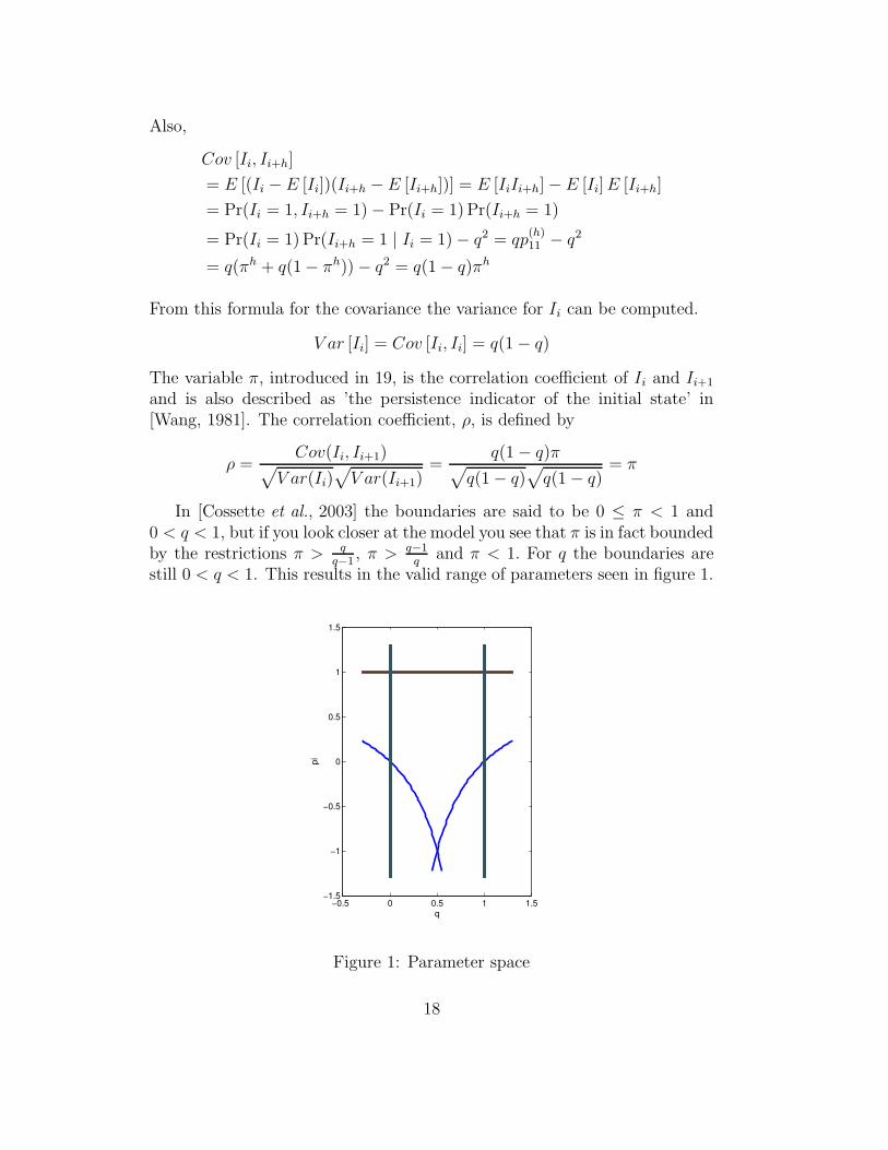
In [Cossette et al., 2003] the boundaries are said to be 0 ≤ π < 1 and0 < q < 1, but if you look closer at the model you see that π is in fact boundedby the restrictions π > q
q−1, π > q−1
qand π < 1. For q the boundaries are
still 0 < q < 1. This results in the valid range of parameters seen in figure 1.
−0.5 0 0.5 1 1.5−1.5
−1
−0.5
0
0.5
1
1.5
q
pi
Figure 1: Parameter space
18

Remark: A more complex model where the process is dependent of two ormore of the previous periods is described in [Isham, 1980].
5.3 The Markov Binomial Model
In this section the number of claims will be further described. The vari-ance and probability mass function will be calculated and the asymptoticdistribution will be examined. The number of claims up to period k, Mk,is the sum of the Markov Bernoulli sequence {Ii : i = 0, . . . , k}. The se-quence {Mk : k = 0, 1, 2, . . .} is called a Markov binomial sequence. If π = 0,Mk ∈ Bin(k, q). The expectation of Mk is
E [Mk] = kq (21)
and the variance is computed by
V ar [Mk] =
k∑
j=1
V ar [Ij] + 2
k−1∑
j=1
k−j∑
h=1
Cov [Ij, Ij+h]
= kq(1 − q) + 2
k−1∑
j=1
k−j∑
h=1
q(1 − q)πh
= kq(1 − q) + 2q(1 − q)π
k−1∑
j=1
1 − πk−j
1 − π
= kq(1 − q) + 2q(1 − q)π
1 − π
(k − 1 −
π(1 − πk−1)
1 − π
)
(22)
So the expectation is unaffected by a possible dependence whereas the vari-ance increases for an increasing π when there is a positive dependence (π > 0)and decreases when |π| increases if there is a negative dependence (π < 0).In figure 2 and figure 3 the variance is plotted from two different angles forall possible values of π and q.
19

−1−0.5
00.5
1
0
0.5
10
100
200
300
400
500
600
piq
Var
ianc
e
Figure 2: The variance for all possible values of π and q
−1 −0.5 0 0.5 100.510
100
200
300
400
500
600
piq
Var
ianc
e
Figure 3: The variance for all possible values of π and q
The conditional and unconditional probability mass functions for Mk,denoted Pr(Mk = j | I0 = i) = pMk
(j | i) and Pr(Mk = j) = pMk(j), have to
20

be computed recursively except the special cases
pMk(0 | i) = pi0 × (p00)
k−1
pMk(k | i) = pi1 × (p11)
k−1(23)
and
pMk(0) = (1 − q) × (p00)
k−1
pMk(k) = q × (p11)
k−1(24)
k ∈ {1, 2, . . .} and i ∈ {0, 1}. Using these special cases all conditional andunconditional probability mass functions can be computed recursively forj ∈ {1, 2, . . . , k − 1} and k ∈ {2, 3, . . .} with
pMk(j | i) = pi0 × pMk−1
(j | 0) + pi1 × pMk−1(j − 1 | 1) (25)
andpMk
(j) = (1 − q) × pMk(j | 0) + q × pMk
(j | 1) (26)
When k goes to infinity the following statement can be used, found in[Cossette et al., 2003].
Let {Ii, i = 0, 1, 2, . . .} be a stationary Markov chain as above. If kq → λand k → ∞, then Mk =
∑ki=1 Ii tends to N where N has a compound
Poisson-Geometric distribution.
N =
∑Kj=1 Zj , K > 0
0 , K = 0
where K is a Poisson distributed random variable with mean (1 − π)λ and{Zj, j = 1, 2, . . .} is a sequence of i.i.d. Geometric distributed random vari-ables independent of K with probability mass function
Pr(Zj = n) = πn−1(1 − π) for n = 1, 2, . . .
The statement holds for π ≥ 0. In [Wang, 1981] the statement is proved, ina way that is relatively easy to understand, by using combinatorics.
The expectation and variance of N are
E[N ] = λ
and
V ar[N ] = λ+ 2λπ
1 − π
21

The probability generating function for N is
G(s) =
exp{−(1 − π)λ
[1 − (1−π)s
1−πs
]}for |s| < π−1, π > 0
exp {−(1 − s)} for all real s, π = 0
which is shown in [Wang, 1981].
5.4 The Compound Markov Binomial Model
In the previous section the properties of Mk, the number of claims up to timek, were described. The next step is to see what happens with the aggregatedclaim amount, Sk =
∑Mk
i=1Xi, when there is a Markov dependency. When{Mk : k = 1, 2, . . .} is a Markov binomial sequence, {Sk : k = 1, 2, . . .}is said to be a compound Markov binomial sequence. Since the sequence ofindividual claim sizes, {Xi : i = 1, 2, . . . , k} consists of i.i.d. random variablesthat are also independent of Mk, the expectation and variance of Sk are easyto find and are given by
E[Sk] = E[Mk]E[X1] (27)
andV ar[Sk] = E[Mk]V ar[X1] + V ar[Mk]E[X1]
2 (28)
In [Cossette et al., 2004] it is suggested that the model could be used forhome insurance in cities where earthquakes are common. A large earthquakeis often followed by smaller earthquakes in the area near the epicenter in thedays after the first earthquake. This means that more claims are expectedto occur, suggesting the kind of dependency described in the model in thiscase with a positive π.
In [Cossette et al., 2003] two ways of computing the probability massfunctions for Sk are proposed. To introduce the first computation the condi-tional and unconditional probability mass functions are defined as
pSk(j | i) = Pr(Sk = j | I0 = i)
andpSk
(j) = Pr(Sk = j) = (1 − q)pSk(j | 0) + qpSk
(j | 1)
for j ∈ {0, 1, 2, . . .} and k ∈ {1, 2, 3, . . .}. From this we can easily obtain
pSk(j | i) =
pMk(0 | i), j = 0
∑kl=1 pMk
(l | i)pX1+X2+...+Xl(j), j = 1, 2, . . .
22

The second way of computation, which will be followed by a proof, is dividedinto two cases. First the case where k = 1
pS1(j | i) =
pi0, j = 0
pi1f(j), j = 1, 2, . . .
and then the recursive formula where the p.m.f. can be computed for k =2, 3, . . ..
pSk(j | i) = pi0pSk−1
(j | 0) + pi1
j∑
l=1
pSk−1(j − l | 1)f(l)
for j = 1, 2, . . .. To prove this a different representation is used for Sk. Let
Yj =
Bj, Ij = 1
0, Ij = 0(29)
where B1, B2, . . . , Bk are i.i.d. random variables distributed as the claimamounts, X. Here Ij (j = 1, 2, . . . , k) and Bj (j = 1, 2, . . . , k) are assumed tobe independent and
Sk = Y1 + . . .+ Yk, (30)
which gives us that
pSk(j | i) = pi0 Pr(Y2 + Y3 + . . .+ Yk = j | I1 = 0)+
+ pi1
j∑
l=1
Pr(Y2 + Y3 + . . .+ Yk = j − l | I1 = 1) Pr(B1 = l)
for k = 2, 3, . . . and j = 1, 2, . . .. The fact that B1 is distributed as X andthe sum Y2 + Y3 + . . .+ Yk is distributed as Sk−1 gives us
pSk(j | i) = pi0 Pr(Sk−1 = j | I1 = 0) + pi1
j∑
l=1
Pr(Sk−1 = j − l | I1 = 1)f(l)
= pi0pSk−1(j | 0) + pi1
j∑
l=1
pSk−1(j − l | 1)f(l).
23

5.4.1 Survival probabilities
In this section the survival probabilities for the compound Markov binomialmodel will be derived, both in finite time and in infinite time. In some ofthe calculations the conditional probabilities will be used to find the uncon-ditional probabilities. Recalling from section 1.1 that x denotes the initialcapital for the portfolio and denoting the surplus of the portfolio by Rk, theconditional survival probabilities can be defined by
φ(x, n | i) = Pr(Rk > 0 ∀k ∈ {1, 2, . . . , n} | I0 = i)
for finite time and
φ(x | i) = Pr(Rk > 0 ∀k ∈ {1, 2, . . .} | I0 = i)
for infinite time. To get the unconditional survival probabilities from theconditional survival probabilities the following relations,
φ(x, n) = qφ(x, n | 1) + (1 − q)φ(x, n | 0)
andφ(x) = qφ(x | 1) + (1 − q)φ(x | 0),
can be used. As mentioned in the introduction the compound Markov bi-nomial model is an extension of the compound binomial model, where thecompound Markov binomial model allows a dependency to exist. The com-pound binomial model, introduced in [Gerber, 1988], can be seen as a specialcase of the compound Markov binomial model, the case where π = 0.
In [Cossette et al., 2003] the survival probabilities for the compound bi-nomial model are derived by
φ(x) =φ(x− 1) − q
∑xj=1 f(j)
1 − q(31)
for x = 1, 2, 3, . . . and
φ(0) =1 − qE(X)
1 − q(32)
for infinite-time and
φ(x, n) = (1 − q)φ(x+ 1, n− 1) + q
x+1∑
j=1
φ(x+ 1 − j, n− 1)f(j) (33)
for x = 0, 1, 2, . . . and n = 1, 2, . . . with
φ(x, 0) = 1 (34)
24

for x = 0, 1, 2, . . . in finite-time. The formulas for finite-time are difficult touse in practice for larger n. The following way to compute the finite-timesurvival probabilities is derived in [Willmot, 1993] and might be easier to usethan (33), if gn(m) = Pr(Sn = m) and Gn(m) = Pr(Sn ≤ m) =
∑mi=1 gn(i)
are not too hard to compute:
φ(x, n) = Gx+n(n) − (1 − q)
k−1∑
m=0
φ(0, n− 1 −m)gx+m+1(m) (35)
φ(0, n) =
∑km=0 Gm(n+ 1)
(1 − q)(n+ 1), k = 0, 1, 2, . . . (36)
In proposition 3 in [Cossette et al., 2003] the following way to recursivelycompute the finite-time survival probabilities for the compound Markov bi-nomial model is derived
φ(x, n | i) = pi0φ(x+ 1, n− 1 | 0) + pi1
x+1∑
j=1
φ(x + 1 − j, n− 1 | 1)f(j) (37)
for x = 0, 1, 2, . . ., n = 1, 2, . . . and i = 0, 1 with
φ(x, 0 | i) = 1 (38)
for x = 0, 1, 2, . . .. This is derived in the same way as (33) and is complicatedto use in practice for larger n. The formula includes φ(x + 1, n− 1 | 0) andto calculate this, φ(x + 2, n − 2 | 0) has to be calculated and so forth, inaddition to calculating φ(a, b | i) for a = 0, 1, . . . , x− 1, b = 1, . . . , n− 1 andi = 0, 1.
The infinite-time survival probabilities conditioned on the first state,
φ(x | 0) =φ(x− 1 | 0) − p01
∑xj=1 φ(x− j | 1)f(j)
p00(39)
for x = 1, 2, 3, . . .,
φ(x | 1) =p10φ(x | 0) + (p00p11 − p01p10)
∑x+1j=2 φ(x + 1 − j | 1)f(j)
p00 − (p00p11 − p01p10)f(1)(40)
for x = 1, 2, 3, . . .,
φ(0 | 0) =1 − qE(X)
1 − q(41)
andφ(0 | 1) =
p10
p00 − (p00p11 − p01p10)f(1)φ(0 | 0) (42)
25

presented in proposition 4 in [Cossette et al., 2003] are easier to use in prac-tice than the finite-time survival probabilities in (37), especially if the initialreserve is low, since survival probabilities do not have to be calculated forinitial reserves larger than x. The proof is included in [Cossette et al., 2003].
5.5 Estimating survival probabilities by simulation
In [Cossette et al., 2003] formulas for deriving finite-time and infinite-timesurvival probabilities are shown, see (37), (39) and (40) in the previous sec-tion. These formulas apply to portfolios of insurance policies where a claimarising from some policy in the portfolio affects the probability of a claimarising from any of the policies in the portfolio in the next period, meaningthat the number of claims for the portfolio is a Markov binomial sequence.In this case the period length is small, maybe a day. If instead the number ofclaims, Mk, for a single insurance policy is a Markov binomial sequence, theformulas can be used to compute the survival probability for one insurance.When looking at a portfolio of insurance policies that are independent ofeach other, but where each insurance policy follows the compound Markovbinomial model, the formulas (37), (39) and (40) can not be used. The finite-time survival probabilities for this kind of portfolio can be estimated by usingsimulation. In the following text a method for simulation is described.
5.5.1 Simulation
Suppose that the portfolio consists of n insurance policies, that are indepen-dent of each other. For simplicity all policies are signed at time 0 when theportfolio is started and none of them are terminated before time k. The finite-time survival probabilities φ(x, t) are estimated for t = 1, 2, . . . , k. Since theindividual claim sizes are independent of the claim occurrences, the MarkovBernoulli sequence and the claim sizes can be simulated separately. To esti-mate φ(x, t) a large number of portfolios have to be simulated.
How to simulate a portfolio and find out if it is ruined in period 1
to k or not:
1) Simulate n k-step Markov chains, here denoted {Aj : j = 1, 2, . . . , n},from the transition matrix (19), where the first step is simulated from aBernoulli random variable with mean q.
2) For each of the n Markov chains, find out the number of 1’s and sim-ulate a claim size to each 1. Be sure to associate each 1 to a specific claim
26

size. Replace each 1 in the Aj’s with the claim size associated with it, theseMarkov chains are denoted {Bj : j = 1, 2, . . . , n}.
3) For i = 1, 2, . . . , k, sum up the i’th step in the Markov chains with theclaims, {Bj : j = 1, 2, . . . , n}. These sums are the total claim amount in eachtime step, which will be denoted {Di : i = 1, 2, . . . , k}. Then calculate thesurplus in period i by
Ri = x+ ci−Wi
where x is the initial capital, c is the premium and
Wi =
i∑
s=1
Ds for i = 1, 2, . . . , k.
4) Create a vector, v, with length k, where element r in the vector is 1if {Ri ≥ 0 for all i = 1, 2, . . . , r} and 0 otherwise. A 1 in element r meansthat the simulated portfolio has carried its costs up until time r and a 0means that it has been ruined.
How to make an estimation of the finite-time survival probabil-
ity through simulation:
5) Repeat 1) - 4) m times to simulate m portfolios. By denoting elementr in the vector v, associated to portfolio i, by ri, the estimation for thesurvival probabilities are
φ(x, r) =
∑mi=1 ri
m.
An extension of 2):The claim sizes can easily be simulated from any distribution. In most math-ematical computer programs it is possible to draw a sample from a U(0,1)-distribution and this sample can then be transformed into a sample fromany given distribution. If a sample is drawn from a continuous distribution,X, the fact that the distribution function, F (X), is U(0,1)-distributed isused. A sample, x, from the desired continuous distribution is generatedby drawing a sample, u, from a U(0,1)-distribution and finding the x thatsolves the equation F (x) = u. To generate a sample from a discrete distri-bution, Y , the same idea is used, but in this case the sample, y, satisfiesPr(X = y − 1) < u ≤ Pr(X = y).
27

6 Maximum likelihood estimations and like-
lihood ratio test
The purpose of this section is to derive the maximum likelihood estimationsfor π and q using the likelihood function for Markov chains, as presented forexample in [Ryden and Lindgren, 2000].
The likelihood function Lx
is the probability of having the observation x,where x can be regarded as one outcome of the random variable X. For aMarkov chain the likelihood function is
Lx
= Pr(X0 = x0, X1 = x1, . . . , Xn = xn)
where x = (x0, x1, . . . , xn) are the n first steps in a Markov chain. Whenusing the Markov Property and the fact that the chain is stationary thelikelihood function is
Lx=(x0,x1,...,xn) = Pr(X0 = x0)
r∏
i=0
r∏
j=0
pnij
ij
where {0, 1, . . . , r} is the state space of the Markov chain and
nij = #{(xk = i, xk+1 = j) : k = 0, 1, . . . , n− 1}
is the number of transitions from state i to state j. If the observation doesnot start in x0, but in a random starting point, xs, in the Markov chain thelikelihood function is
Lx
=r∏
i=0
r∏
j=0
pnij
ij
which is more or less the same, only now x = (xs, xs+1, . . . , xs+n). Themaximum likelihood estimation of a set of parameters θ is the estimationthat maximizes the likelihood function for the observation x.
For a deeper, more general, explanation of the likelihood function andmaximum likelihood estimations, see [Azzalini, 1996].
6.1 Maximum likelihood estimations for the variables
in the compound Markov binomial model
To derive the maximum likelihood estimations for π, q and q0, where q0 =Pr(X0 = 1), when the data consists of a number of observations from different
28
Markov chains, with the same distribution, the likelihood function for theentire data material is
L =
N1+N2∏
k=1
Lk = (1 − q0)N0qN1−N0
0
N1∏
i=k
pnk
00
00 pnk
01
01 pnk
10
10 pnk
11
11
N1+N2∏
k=N1+1
pnk
00
00 pnk
01
01 pnk
10
10 pnk
11
11
= (1 − q0)N0qN1−N0
0
N1+N2∏
k=1
pnk
00
00 pnk
01
01 pnk
10
10 pnk
11
11 .
(43)
Here, N1 is the number of observed Markov chains where the observationstarts when the chain begins and N0 is the number of these that start in 0.The variable N2 is the number of observed Markov chains beginning beforethe starting point of the observation. The number of transitions from i to jobserved for the k’th Markov chain is denoted by nk
ij, for i, j = {0, 1}. Recallthat the transition probabilities are given by the following matrix,
P =
(p00 p01
p10 p11
)=
(1 − (1 − π)q (1 − π)q
(1 − π)(1 − q) π + (1 − π)q
).
Replacing p00, p01, p10 and p11 with their parameterizations in terms of π andq we obtain
L(q0, q, π) =
N1+N2∏
k=1
Lk(q0, q, π) = (1 − q0)N0qN1−N0
0 ×
×N1+N2∏
k=1
[(1 − (1 − π)q)nk
00((1 − π)q)nk01((1 − π)(1 − q))nk
10(π + (1 − π)q)nk11
]
(44)
Taking the logarithm of the likelihood function makes it easier to handle.Since the log likelihood function and the likelihood function have the samemaximum points the log likelihood can be used to get the same maximumlikelihood estimations. We obtain
lgL =N0 lg(1 − q0) + (N1 −N0) lg q0+
+
N1+N2∑
k=1
[nk00 lg(1 − (1 − π)q) + nk
01 lg((1 − π)q)+
+ nk10 lg((1 − π)(1 − q)) + nk
11 lg(π + (1 − π)q)].
(45)
Differentiating (45) with respect to q0, q and π gives us
∂(lgL)
∂q0= −
N0
1 − q0+N1 −N0
q0= 0 (46)
29

∂(lgL)
∂q=
N1+N2∑
i=k
(−(1 − π)nk
00
1 − q(1 − π)+nk
01
q+
(−1)nk10
1 − q+
(1 − π)nk11
π + (1 − π)q
)= 0
(47)
∂(lgL)
∂π=
N1+N2∑
k=1
(qnk
00
1 − q(1 − π)+
(−1)nk01
1 − π+
(−1)nk10
1 − π+
(1 − q)nk11
π + (1 − π)q
)= 0
(48)From (46) the maximum likelihood estimation for q0,
q0 =N1 −N0
N1, (49)
is obtained. By denoting n00 =∑N1+N2
k=1 nk00, n01 =
∑N1+N2
k=i nk01, n10 =∑N1+N2
k=1 nk10 and n11 =
∑N1+N2
k=1 nk11, and rearranging (47) and (48) we obtain
n01 + n10
1 − π=
n00q
1 − (1 − π)q+
n11(1 − q)
π + (1 − π)q(50)
andn10
1 − q−n01
q=
n11(1 − π)
π + (1 − π)q−
n00(1 − π)
1 − (1 − π)q. (51)
Rearranging (50) results in
n01 + n10 =n11(1 − π)
π + (1 − π)q− q (
n11(1 − π)
π + (1 − π)q−
n00(1 − π)
1 − (1 − π)q)
︸ ︷︷ ︸Right hand side of (51)
(52)
By inserting (51) in (52) and simplifying it is seen that
n10
1 − q=
n11(1 − π)
π + (1 − π)q,
which gives the result
q = 1 −n10
(1 − π)(n10 + n11). (53)
By inserting (53) in (51) and simplifying the following log likelihood estimatefor π,
π = 1 −n01
n00 + n01−
n10
n11 + n10, (54)
30

is derived and by using (54) the estimate for q is
q =n01
n00 + n01/(
n10
n11 + n10+
n01
n00 + n01). (55)
So the maximum likelihood estimations for the parameters π, q and q0 are
π = 1 − n01
n00+n01
− n10
n11+n10
q = n01
n00+n01
/( n10
n11+n10
+ n01
n00+n01
)
q0 = N1−N0
N1
(56)
Remark 1: The log likelihood function can also be derived with respect tothe transition probabilities p00, p01, p10 and p11, instead of π and q, and thenuse for example p01 and p10 to retrieve the same estimations for π and q.Remark 2: Assuming that there is no dependency, π = 0, the likelihoodfunction is
L(q0, q) =
N1+N2∏
k=1
Lk(q0, q)
= (1 − q0)N0qN1−N0
0
N1+N2∏
k=1
[(1 − q)nk
00qnk01(1 − q)nk
10qnk11
] (57)
and the maximum likelihood estimation for q0 is still (49) and for q theestimate is
qind =n01 + n11
n00 + n01 + n10 + n11(58)
6.1.1 Confidence intervals
In [Ryden and Lindgren, 2000] the formula
pij ± zα/2
√pij(1 − pij)/ni (59)
for calculating confidence intervals for the maximum likelihood estimationsof the transition probabilities with approximated confidence level (1 − α)is derived, where zα is the (α/2)-quantile of the N(0,1)-distribution andni = ni0 + ni1. The confidence interval for pij is constructed in the sameway as a confidence interval for the maximum likelihood estimation of p fora Bin(n, p)-variable, with the difference that instead of a fixed n in the bi-nomial case there is the random number ni.
31

6.2 Likelihood ratio test using the bootstrap method
In [Azzalini, 1996] the likelihood ratio test is defined as testing the two al-ternatives
{H0 : θ∗ ∈ Θ0
H1 : θ∗ ∈ Θ1
where θ ∈ Θ = Θ0 ∪ Θ1, using the likelihood ratio
λ(x) =supθ∈Θ0
L(θ;x)
supθ∈Θ L(θ;x)
where x is a vector consisting of the observed values from the random variableX = {X1, X2, . . . , Xn} and L(θ) is assumed to be continuous for all possiblevalues of x. The null hypothesis H0 is rejected at level α if λ(x) is in therejection area
R = {x : λ(x) ≤ λα}
with λα chosen so that
supθ∈Θ0
Pr(λ(X) ≤ λα; θ) = α.
To see if there is no dependence in the model the hypothesis
{H0 : π = 0, q ∈ [0, 1]
H1 : π 6= 0, q ∈ [0, 1]
can be tested using the Likelihood ratio test. For this test θ = {π, q} andthe likelihood ratio is
λ(x) =L(θH0
;x)
L(θH1;x)
=L(0, qind;x)
L(π, q;x). (60)
where x = (n00, n01, n10, n11). Instead of trying to find λα theoretically, whichis often difficult, we decided to use the bootstrap method to find the rejectionarea.
The general idea with a bootstrap method is to estimate the parameters ofa model and then use the estimators to simulate a new data set and comparethis with the original data set. An experiment is carried out to get a dataset from X, which will be denoted x = (x1, x2, . . . , xn). In this model the x
32

is represented by a Markov chain and θ is the set of {π, q, qind}. B randomsamples of a Markov chain are simulated from the estimated transition matrix
P =
(p00 p01
p10 p11
),
these Markov chains are denoted
x∗j = (x∗1j , x
∗2j , . . . , x
∗nj)
for j = 1, 2, . . . , B, and they are called the bootstrap samples. From x∗j the
bootstrap replications of θ will be calculated and will be denoted
θ(x∗1), θ(x
∗2), . . . , θ(x
∗B)
and the bootstrap replications of λ are denoted
λ∗j = λ(x∗j) =
L(0, qind∗j ;x
∗j)
L(π∗j , q
∗j ;x
∗j)
for j = 1, 2, . . . , B. A p-value, p = Pr(λ∗ < λ), to be used in the likelihoodratio test is estimated by using the estimator
p∗ =#{j ∈ {1, 2, . . . , B} : λ∗
j < λ}
B.
To reject H0 at level α the estimated p-value should be at most 1 − α.For a more general description of the bootstrap method see [Hastie et al., 2001].
33
7 Fitting data to the compound Markov bi-
nomial model
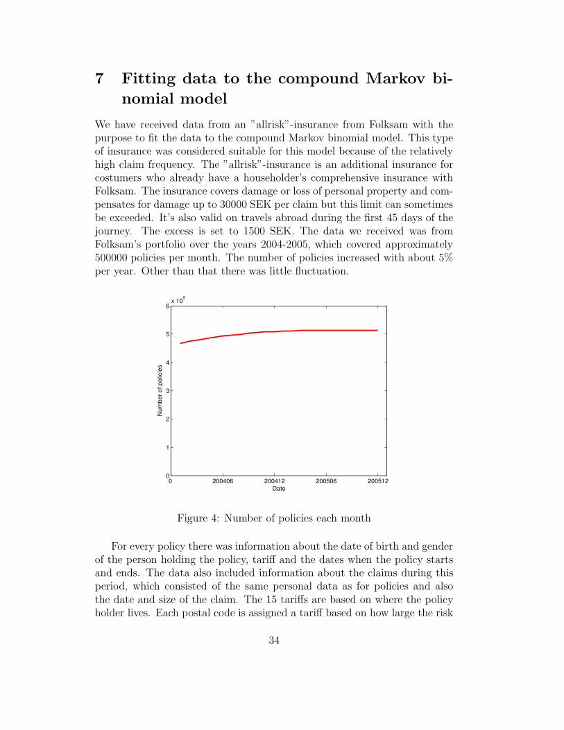
We have received data from an ”allrisk”-insurance from Folksam with thepurpose to fit the data to the compound Markov binomial model. This typeof insurance was considered suitable for this model because of the relativelyhigh claim frequency. The ”allrisk”-insurance is an additional insurance forcostumers who already have a householder’s comprehensive insurance withFolksam. The insurance covers damage or loss of personal property and com-pensates for damage up to 30000 SEK per claim but this limit can sometimesbe exceeded. It’s also valid on travels abroad during the first 45 days of thejourney. The excess is set to 1500 SEK. The data we received was fromFolksam’s portfolio over the years 2004-2005, which covered approximately500000 policies per month. The number of policies increased with about 5%per year. Other than that there was little fluctuation.
0 200406 200412 200506 2005120
1
2
3
4
5
6x 10⁵
Date
Num
ber o
f pol
icie
s
Figure 4: Number of policies each month
For every policy there was information about the date of birth and genderof the person holding the policy, tariff and the dates when the policy startsand ends. The data also included information about the claims during thisperiod, which consisted of the same personal data as for policies and alsothe date and size of the claim. The 15 tariffs are based on where the policyholder lives. Each postal code is assigned a tariff based on how large the risk
34
is considered to be for a person from that particular area to have a claim.An area with a high risk of a claim is given a high tariff number. The priceof the insurance is based on where the policy holder lives and if he or sheis under 60 years old or not, with an average price of 450 SEK per year. Insection 7.1 we will further examine the claims in the data set. The numberof claims and the claim sizes will be plotted and described. The distributionfor the claim sizes will also be discussed in this section. In section 7.2 we willdescribe the estimations of the parameters in the compound Markov binomialmodel for the whole data material, when the zero-claims are excluded andwhen the data material is divided into separate groups for men and women.Furthermore a likelihood ratio test will be implemented for the hypothesisthat π = 0 and confidence intervals for pij will be calculated.
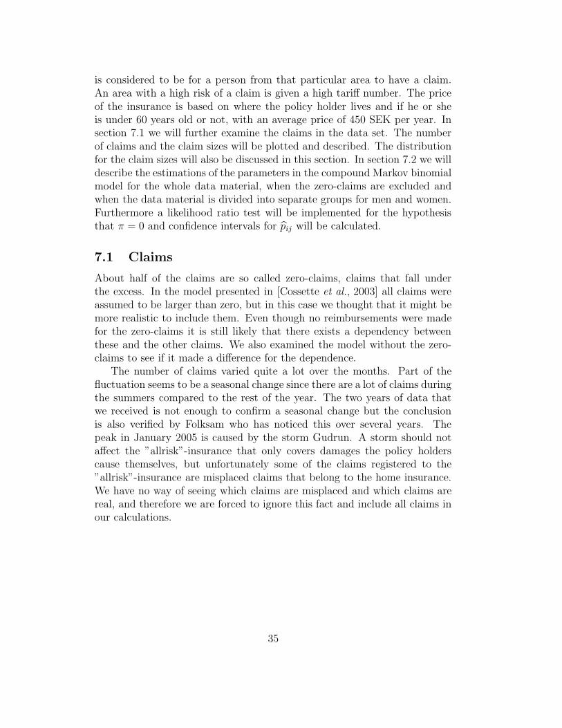
7.1 Claims
About half of the claims are so called zero-claims, claims that fall underthe excess. In the model presented in [Cossette et al., 2003] all claims wereassumed to be larger than zero, but in this case we thought that it might bemore realistic to include them. Even though no reimbursements were madefor the zero-claims it is still likely that there exists a dependency betweenthese and the other claims. We also examined the model without the zero-claims to see if it made a difference for the dependence.
The number of claims varied quite a lot over the months. Part of thefluctuation seems to be a seasonal change since there are a lot of claims duringthe summers compared to the rest of the year. The two years of data thatwe received is not enough to confirm a seasonal change but the conclusionis also verified by Folksam who has noticed this over several years. Thepeak in January 2005 is caused by the storm Gudrun. A storm should notaffect the ”allrisk”-insurance that only covers damages the policy holderscause themselves, but unfortunately some of the claims registered to the”allrisk”-insurance are misplaced claims that belong to the home insurance.We have no way of seeing which claims are misplaced and which claims arereal, and therefore we are forced to ignore this fact and include all claims inour calculations.
35

0 200406 200412 200506 2005120
500
1000
1500
2000
2500
3000
3500
4000
4500
Date
Num
ber o
f cla
ims
Figure 5: Number of claims each month
As can be seen by comparing figure 5 with figure 6 the frequency of thenumber of claims, which is computed by dividing the number of claims bythe number of policies, follows the same pattern as the number of claims.
0 200406 200412 200506 2005120
0.001
0.002
0.003
0.004
0.005
0.006
0.007
0.008
0.009
0.01
Date
Cla
im fr
eque
ncy
Figure 6: Claim frequency
36

In figure 7 the number of non-zero claims each month are plotted. Sincethe peak in January 2005 consists of a lot of claims that do not really belongto this insurance this peak is smaller when the zero-claims are removed.
200406 200412 200506 2005120
500
1000
1500
2000
2500
Date
Num
ber o
f cla
ims
Figure 7: Number of non-zero claims per month
The sizes of the claims are often estimated by a logarithmic distributionwhen they are said to have a discrete distribution as in [Cossette et al., 2003].We will define the probability mass function for the logarithmic distributionby
f(k) = −rk
k × log(1 − r)
where r will be equivalent to β1+β
in the definition of the probability mass
function in [Cossette et al., 2003]. Given that Y is a random variable with alogarithmic distribution the expected value of Y is
E [Y ] =−r
(1 − r)log(1 − r)
In reality the claim sizes have a continuous distribution but to match themodel, in which the claims sizes are said to be discrete variables, the empiricaldistribution is transformed into a discrete distribution. First we made enempirical distribution for the sizes of the original claim, without subtractingthe excess of 1500 SEK. This is done by putting all the zero-claims into the
37

first interval, these are all the claims that originally had a size between 1and 1500 SEK, and then adding 1500 SEK to the non-zero claim sizes anddividing them into unit intervals of 1500 SEK. In the bar graph in figure8 this discrete empirical distribution, X, is shown as the dark bars. Basedon the intervals the mean that should be used to estimate the parameter rwill be 2.2756 units, which corresponds to 3413.4 SEK, and this gives us anestimated value for r of
r = 0.7696.
As can be seen in figure 8 the empirical distribution follows the logarithmicdistribution fairly well but in the interval 30000-31500 SEK the empiricaldistribution is a lot higher than the logarithmic distribution. This area isblown up in figure 9. The limit for reimbursement is 30000 SEK so largerclaims will be reduced to 30000 SEK. This means that the damages shownas 30000 SEK in the data material might in fact be larger and this makesthe probability of a claim of this size larger in the empirical distribution thanin reality. This limit is sometimes exceeded which explains that some of theclaim sizes are larger than 30000 SEK. The probability that a claim will behigher than 30000 SEK is 0.0005 for the logarithmic distribution while thesame probability for the empirical distribution is 0.0027. This implies thatthe empirical distribution has a heavier tail than the logarithmic distribution.
6750 14250 21750 29250 367500
0.1
0.2
0.3
0.4
0.5
0.6
0.7
Claim size interval
Pro
babi
lity
Figure 8: Distribution function for the claim sizes
38

29250 30750−0.02
−0.015
−0.01
−0.005
0
0.005
0.01
0.015
0.02
Claim size interval
Pro
babi
lity
Figure 9: Distribution function for the claim sizes
The distribution for the claim sizes without zero-claims does not followthe logarithmic distribution as well as when the zero-claims are included sowe plotted it without a fitted logarithmic distribution.
6750 14250 21750 29250 367500
0.05
0.1
0.15
0.2
0.25
0.3
0.35
0.4
0.45
Claim size interval
Pro
babi
lity
Figure 10: Distribution function for the claim sizes without zero claims
7.2 Estimations
To make the estimations we decided to first use the period length of 182days, which is about six months. We first wanted to try with a long period
39

to maximize the chance of finding a dependency. On the other hand weonly had two years of data and we needed to have at least a few transitionsduring this time to make the estimation reliable. We also wanted to trywith a shorter period to have more transitions so we decided to use a periodof 60 days. When using 182 days interval this gave us a maximum of 3transitions and using 60 days gave us a maximum of 11 transitions. Thesame estimations were made first with the zero-claims included in the datamaterial, then again without the zero-claims.
7.2.1 The maximum likelihood estimations
Applying (56) in section 6.1 gives us the estimations for π, q and q0. If weinstead assume that there is no dependency, π = 0, and apply (58) we getthe estimation for qind, while q0 is the same as in the case with dependency.Doing this for the period lengths 182 days and 60 days and for the data in-cluding the zero-claims and the data excluding the zero-claims gives us table1.
Including zero-claims Excluding zero-claims60 days 182 days 60 days 182 days
q0 0.0193 0.0505 0.0102 0.0272q 0.0119 0.0342 0.0062 0.0178π 0.0138 0.0391 0.0078 0.0256qind 0.0119 0.0343 0.0062 0.0179
Table 1: Maximum likelihood estimations
Remark 1: As would be expected q is more or less the same as qind inall four cases.Remark 2: When the estimations of the correlation coefficient π are thissmall one might think that the dependency has little effect but since theclaim frequency is also low the dependency actually has a significant effecton the transition probabilities.Remark 3: The total amount of transitions in the data material was 5061892for periods of 60 days and 1128800 for periods of 182 days when the zero-claims were included. Excluding the zero-claims gave us 5120435 transitionsfor periods of 60 days and 1166089 transitions for periods of 182 days.
40

The maximum likelihood estimation of the transition matrix are
When the zero-claims were included in the data material
For periods of 182 days
P =
(p00 p01
p10 p11
)=
(0.9671 0.03290.9280 0.0720
)
This can be compared to the case when π = 0 where p00 = p10 = 0.9657 andp01 = p11 = 0.0343.
For periods of 60 days
P =
(p00 p01
p10 p11
)=
(0.9883 0.01170.9745 0.0255
)
In the case when π = 0 the estimated transition probabilities are p00 = p10 =0.9881 and p01 = p11 = 0.0119. For both period lengths the estimation of p11
is more than twice as large as p01. This suggests that it is more likely that apolicy holder who has had a claim in the previous period will have a claimin this period than a policy holder who has not had a claim in the previousperiod.
When the zero-claims were excluded from the data material
For periods of 182 days
P =
(p00 p01
p10 p11
)=
(0.9827 0.01730.9571 0.0429
)
This can be compared to the case when π = 0 where p00 = p10 = 0.9822 andp01 = p11 = 0.0178.
For periods of 60 days
P =
(p00 p01
p10 p11
)=
(0.9938 0.00620.9860 0.0140
)
In the case when π = 0 the estimated transitions probabilities are p00 =p10 = 0.9938 and p01 = p11 = 0.0062. When the zero-claims were excludedfrom the data the difference between p01 and p11 became even larger sinceπdid not decrease in the same degree as q.
41

We estimated q, π, q0 and qind for men and women separately to see ifthere was a difference between the two groups. The result if found in table2 and table 3.
Including zero-claims Excluding zero-claims60 days 182 days 60 days 182 days
q0 0.0188 0.0496 0.0102 0.0271q 0.0114 0.0329 0.0061 0.0175π 0.0134 0.0367 0.0080 0.0258qind 0.0115 0.0329 0.0061 0.0176
Table 2: Maximum likelihood estimations for men
Including zero-claims Excluding zero-claims60 days 182 days 60 days 182 days
q0 0.0309 0.0364 0.0102 0.0272q 0.0124 0.0357 0.0063 0.0182π 0.0140 0.0416 0.0076 0.0253qind 0.0125 0.0358 0.0063 0.0182
Table 3: Maximum likelihood estimations for women
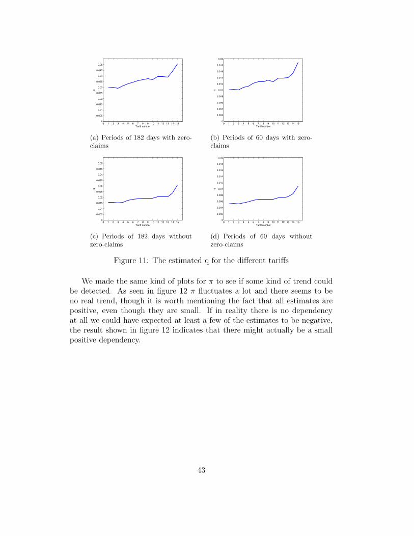
We plotted the estimated q for each tariff to see if Folksam’s classificationwith tariffs was fair. In figure 11 it shows that though there are some fluc-tuations q has a clear up going trend for increasing tariff numbers for bothperiod lengths. Therefore it seems to be correct that a person with a hightariff number will have a higher risk of having a claim than a person with alower tariff number.
42
0 1 2 3 4 5 6 7 8 9 10 11 12 13 14 150
0.005
0.01
0.015
0.02
0.025
0.03
0.035
0.04
0.045
0.05
Tariff number
q
(a) Periods of 182 days with zero-claims
0 1 2 3 4 5 6 7 8 9 10 11 12 13 14 150
0.002
0.004
0.006
0.008
0.01
0.012
0.014
0.016
0.018
0.02
Tariff number
q
(b) Periods of 60 days with zero-claims
0 1 2 3 4 5 6 7 8 9 10 11 12 13 14 150
0.005
0.01
0.015
0.02
0.025
0.03
0.035
0.04
0.045
0.05
Tariff number
q
(c) Periods of 182 days withoutzero-claims
0 1 2 3 4 5 6 7 8 9 10 11 12 13 14 150
0.002
0.004
0.006
0.008
0.01
0.012
0.014
0.016
0.018
0.02
Tariff number
q
(d) Periods of 60 days withoutzero-claims
Figure 11: The estimated q for the different tariffs
We made the same kind of plots for π to see if some kind of trend couldbe detected. As seen in figure 12 π fluctuates a lot and there seems to beno real trend, though it is worth mentioning the fact that all estimates arepositive, even though they are small. If in reality there is no dependencyat all we could have expected at least a few of the estimates to be negative,the result shown in figure 12 indicates that there might actually be a smallpositive dependency.
43

0 1 2 3 4 5 6 7 8 9 10 11 12 13 14 150
0.01
0.02
0.03
0.04
0.05
0.06
0.07
Tariff number
pi
(a) Periods of 182 days with zero-claims
0 1 2 3 4 5 6 7 8 9 10 11 12 13 14 150
0.002
0.004
0.006
0.008
0.01
0.012
0.014
0.016
0.018
0.02
Tariff number
pi
(b) Periods of 60 days with zero-claims
0 1 2 3 4 5 6 7 8 9 10 11 12 13 14 150
0.01
0.02
0.03
0.04
0.05
0.06
0.07
Tariff number
pi
(c) Periods of 182 days withoutzero-claims
0 1 2 3 4 5 6 7 8 9 10 11 12 13 14 150
0.002
0.004
0.006
0.008
0.01
0.012
0.014
0.016
0.018
0.02
Tariff number
pi
(d) Periods of 60 days withoutzero-claims
Figure 12: The estimated π for the different tariffs
7.2.2 Likelihood ratio test
The likelihood ratio, λ, for testing the hypothesis{H0 : π = 0
H1 : π 6= 0
is calculated with (60) in which (57), where q = qind, is divided by (44),where π = π and q = q. For the data material λ is
λ182,I = 0
for the 182 day-period andλ60,I = 0
for the 60 day-period when the zero-claims were included and
λ182,E = 0
for the 182 day-period andλ60,E = 0
44

for the 60 day-period when the zero-claims were excluded. For each case 1000bootstrap replications of λ were made. We wanted to use the same lengthof time for all the simulations and therefore made replications by simulating10000-step Markov chains for the 182-day periods and 30000-step Markovchains for the 60-day periods. This was done by using the transition matrix
Pind =
((1 − qind) qind
(1 − qind) qind
).
Then π, q, qind and finally λ were calculated for these chains. Finally
p∗ =#{i : λ∗i < λ}
B
were calculated, which isp∗182,I = 0
for periods with a length of 182 days, and
p∗60,I = 0
for periods of 60 days when the zero-claims were included and
p∗182,E = 0
for periods with a length of 182 days, and
p∗60,E = 0
for periods of 60 days when the zero-claims were excluded.The smallest value of the λ∗
i ’s was 0.0013 for the interval of 182 days and0.0101 for the interval of 60 days when the zero-claims were included and0.0024 for the interval of 182 days and 0.0020 for the interval of 60 dayswhen the zero-claims were excluded. This means that even though λ60,I ,λ182,I , λ60,E and λ182,E were rounded off to zero none of the λ∗
i ’s were evenclose to falling below the λ’s calculated for the data material since the largestone was in order 10−55. This means that H0 can be rejected in all cases.
45
7.2.3 Confidence intervals
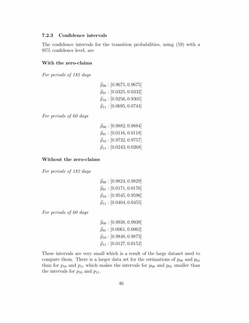
The confidence intervals for the transition probabilities, using (59) with a95% confidence level, are
With the zero-claims
For periods of 182 days
p00 : [0.9675, 0.9675]
p01 : [0.0325, 0.0332]
p10 : [0.9256, 0.9305]
p11 : [0.0695, 0.0744]
For periods of 60 days
p00 : [0.9882, 0.9884]
p01 : [0.0116, 0.0118]
p10 : [0.9732, 0.9757]
p11 : [0.0243, 0.0268]
Without the zero-claims
For periods of 182 days
p00 : [0.9824, 0.9829]
p01 : [0.0171, 0.0176]
p10 : [0.9545, 0.9596]
p11 : [0.0404, 0.0455]
For periods of 60 days
p00 : [0.9938, 0.9939]
p01 : [0.0061, 0.0062]
p10 : [0.9848, 0.9873]
p11 : [0.0127, 0.0152]
These intervals are very small which is a result of the large dataset used tocompute them. There is a larger data set for the estimations of p00 and p01
than for p10 and p11 which makes the intervals for p00 and p01 smaller thanthe intervals for p10 and p11.
46

7.2.4 Stationarity
We wanted to test the stationarity of the material. We therefore estimatedq0 so it could be compared with q. In all cases q0 is much larger than q sowe decided to estimate {qi, i = 1, 2, 3, 4}, the probability of a claim in periodi after the insurance policy is signed. By estimating {qi, i = 1, 2, 3, 4} wewanted to see if the probability of a claim during the first period seemedto drop toward q. We only looked at the set of insurances that were signedduring 2004-2005 and that were at least four periods long. This could onlybe done for the interval of 60 days since the data material would be too smallwhen using an interval of 182 days. We estimated qi by
qi =ni
N
where ni is the number of claims in period i and N is the total number ofinsurances. Using this formula gave us the following estimations when thezero-claims were included
q1 = 0.0213, q2 = 0.0173, q3 = 0.0134, q4 = 0.0122.
When the zero-claims were excluded the estimations were
q1 = 0.0102, q2 = 0.0093, q3 = 0.0081, q4 = 0.0075.
This shows that the number of claims decreases with time. The fact that q1
is higher than q2, q3 and q4 shows that there is a higher risk of a claim in thefirst period than in the later periods and that motivates the use of q0 in sec-tion 6.1. The result indicated that the Markov chain might not be stationaryand that the probability of a claim instead is decreasing with time. The fastdrop during the first periods toward q also indicated that the Markov chainmight only lack stationarity in the first periods and then stabilize.
7.2.5 Probability of survival
The net profit condition for the data is
qE [X] < c.
According to Folksam the average premium is 450 SEK per year, this cor-responds to a premium of 225 SEK for periods of 182 days and 75 SEK forperiods of 60 days. For all the estimations we have made, this premiumis much higher than the estimations of the expected reimbursement each
47

period, qE [X], about four times as high. Insurance companies are an impor-tant part of society’s safety net and can not be allowed to risk bankruptcy,therefore it is crucial that the insurance companies take out premiums thatmore than satisfies the net profit condition. The survival probability of the”allrisk”-insurance portfolio can, since the premium is much higher than theexpected cost, be expected to be 1. To check this we made a simulation ofthe survival probability, using the method in section 5.5.1. The choice ofperiod length and whether the zero-claims are included or not should nothave an affect on the survival probability, therefore we only simulated thesurvival probability of a portfolio using the estimations for a period length of182 days including the zero claims. The simulation was done for a portfolioof 1000 insurance policies, in 100 time steps which corresponds to 50 years.To simulate the claim sizes we used the empirical distribution shown as thedark bars in figure 8. 1000 portfolios where simulated, all of them survived,meaning that they all had a surplus higher than or equal to zero in all the100 time steps. The estimated survival probability is therefore 1 as expected.
48

8 Discussion
We have studied some dependency models in non-life insurance. There existquite a few models for describing different types of dependence, in this paperwe have presented four different models, but they are all very theoretical andsometimes hard to implement. Out of the four models we have described,the model with dependency between classes of business and groups of eventsin section 2 and the copula model in section 3 are more general since theydo not have any restrictions on the distributions of the random variables inthe models.
The model with dependency between classes of business and groups ofevents in section 2 can in theory be used for an insurance company’s wholeportfolio, but it is so extensive that it is hard to implement practically, es-pecially the classification makes the model very hard to use since misclassi-fication can have a large effect on the ruin probability.
The copula model in section 3 can quite easily be used for insurance typeswith dependence between claim sizes. With an empirical distribution or awell fitted distribution and estimated covariance for the claim sizes the ruinprobability is easy to simulate using the copula model. The disadvantagewith this model is that [Albrecher, 1998] does not derive any test to see howaccurate these ruin probabilities are.
The model with dependency between claim sizes and claim intervals insection 4 and the compound Markov binomial model, in section 5, are veryspecific and therefore it is hard to find a type of insurance that will fit thesemodels. The advantage of these models is that there exist formulas for com-puting the ruin probabilities, while for the model with dependency betweenclasses of business and groups of events, in section 2, there are only upperbounds for the ruin probabilities and for the copula model, in section 3, theruin probabilities have to be simulated.
The model with dependency between claim sizes and claim intervals insection 4 is an interesting model but it is hard to find insurance types forwhich it is suitable, partly because of the special type of dependence andpartly because of the restriction of the distributions. There are no examplesof situations, in [Albrecher and Boxma, 2004], for when the model can beimplemented.
The focus of this paper has been on the compound Markov binomialmodel and fitting its parameters to the ”allrisk”-insurance. The dependencebetween claim occurrences in this model is easy to use in practice, as we havedone for the data from the ”allrisk”-insurance, even tough we had to makesome adjustments. Since the model is discrete and only allows one claimin each period we have had to ignore the fact that in some periods there
49
were two or more claims and instead regard them as one claim. In non-lifeinsurance the claim sizes are usually considered to be continuous which makesit easier to find a suitable distribution that fits the data. The only discretedistribution we have found that might fit insurance claims is the logarithmicdistribution which did not fit the data from the ”allrisk”-insurance when thezero-claims were excluded.
As shown in section 7.2.5 the stationarity assumption in the compoundMarkov binomial model is not entirely fulfilled for the data. There seemsto be a lack in stationarity when the policy is first signed. There is also aseasonal change in the claim probability, which i shown in figure 6 in section7.1. The seasonal change does however not have to be a problem if theperiod length is set to a year, which is a quite natural period length sincemost insurance policies are signed for a year at a time. The only reason whywe have not made any estimations for period lengths of one year is becausethe data only covered two years of time, which is too small to make this kindof estimations.
The estimations we have made when fitting the data from the ”allrisk”-insurance to the Markov Bernoulli model show that the probability for apolicy holder to have a claim in period i is about twice as high if the policyholder has had a claim in period i− 1 than if period i− 1 is claim free. Thisresult may lead one to think that it would be a good idea for the insurancecompany to raise the premium in period i when a claim has occurred in theprevious period, and lower it otherwise, to get a more fair pricing while thetotal premium amount for the entire portfolio remains the same. However,since the probability of a claim is very low for this type of insurance policythe increase in premium for those who had a claim in period i−1 will be highwhile those without a claim will get a very small decrease in premium. It istherefore unwise to make this kind of premium adjustment, the negative effectfor those getting a higher premium would be significant while the positiveeffect for those getting a decrease would be almost unnoticeable.
50

References
[Albrecher and Boxma, 2004] H. Albrecher and O. J. Boxma. A ruin modelwith dependence between claim sizes and claim intervals. Insurance: Math-
ematics and Economics, (35):245–254, 2004.
[Albrecher, 1998] H. Albrecher. Dependent risks and ruin probabilities ininsurance. International Institute for Applied Systems Analysis, 1998.
[Azzalini, 1996] A. Azzalini. Statistical Inference. Chapman and Hall, 1996.
[Cossette et al., 2003] H. Cossette, D. Landriault, and E. Marceau. Ruinprobabilities in the compound binomial model. Scandinavian Actuarial
Journal, (4):301–323, 2003.
[Cossette et al., 2004] H. Cossette, D. Landriault, and E. Marceau. Exact ex-pressions and upper bound for ruin probabilities in the compound markovbinomial model. Insurance: Mathematics and Economics, (3):449–466,2004.
[Gerber, 1988] H. Gerber. Mathematical fun with ruin theory. Insurance:
Mathematics and Economics, (7):15–23, 1988.
[Gut, 1995] A. Gut. An Intermediate Course in Probability. Springer, NewYork, 1995.
[Hastie et al., 2001] T. Hastie, R. Tibshirani, and J. Friedman. The Elements
of Statistical Learning. Springer, New York, 2001.
[Isham, 1980] V. Isham. Dependent thinning of point processes. Journal of
Applied Probability, (17):987–995, 1980.
[Klaassen and Wellner, 1997] C. A. J. Klaassen and J. A. Wellner. Efficientestimation in the bivariate normal copula model: Normal margins are leastfavourable. Bernoulli Journal, (1):55–77, 1997.
[Nelsen, 2006] R. B. Nelsen. An Introduction to Copulas. Springer, NewYork, 2006.
[Ryden and Lindgren, 2000] T. Ryden and G. Lindgren. Markovprocesser.Lund University, 2000.
[Wang and Yuen, 2005] G. Wang and K. C. Yuen. On a correlated aggregateclaims model with thinning-dependence structure. Insurance: Mathemat-
ics and Economics, (36):456–468, 2005.
51

[Wang, 1981] Y. H. Wang. On the limit of the markov binomial distribution.Journal of Applied Probability, (18):937–942, 1981.
[Willmot, 1993] G. E. Willmot. Ruin probabilities in the compound binomialmodel. Insurance:Mathematics and Economics, (12):133–142, 1993.
52