Quasinormal modes of magnetic and electric black branes versus

far from equilibrium anisotropic fluids

Stefan Janiszewski∗

Department of Physics and Astronomy,

University of Victoria, Victoria, BC, V8P 5C2, Canada

Matthias Kaminski†

Department of Physics and Astronomy,

University of Alabama, Tuscaloosa, AL 35487, USA

(Dated: January 19, 2016)

Abstract

Detailed knowledge about equilibration processes is of interest for various fields of physics, in-

cluding heavy ion collision experiments and quantum quenched condensed matter systems. We

study the approach to equilibrium at late times within two types of strongly coupled thermal

systems in 3 + 1 dimensions: systems in the presence of (i) a non-zero charge density, or (ii) a

magnetic field at vanishing charge density. Utilizing the gauge/gravity correspondence, we map

the aforementioned problem to the computation of quasinormal frequencies around two particular

classes of black branes within the Einstein-Maxwell theory. We compute (i) the tensor and vec-

tor quasinormal modes of Reissner-Nordstrom black branes and (ii) the scalar, as well as tensor

quasinormal modes of magnetic black branes. Some of these quasinormal modes correspond to the

late-time relaxation of the above systems after starting with initial pressure anisotropy. We provide

benchmarks which need to be matched at late-times by all holographic thermalization codes with

the appropriate symmetries.

∗Electronic address: stefanjj@uvic.ca†Electronic address: mski@ua.edu

1

arX

iv:1

508.

0699

3v2

[he

p-th

] 1

6 Ja

n 20

16

Contents

I. Introduction 2

II. Far from equilibrium setups & quasinormal modes 6

III. Holographic setup 8

A. Reissner-Nordstrom black branes 8

1. Equilibrium solutions and thermodynamics 9

2. Fluctuations 11

B. Magnetic black branes 13

1. Equilibrium solutions and thermodynamics 13

2. Fluctuations 19

IV. Computational methods 21

A. Shooting 21

B. Continued fractions 22

1. Pincherle’s theorem 23

2. Application to Reissner-Nordstrom 23

V. Results 25

A. Quasinormal frequencies of Reissner-Nordstrom black branes 26

B. Quasinormal frequencies of magnetic black branes 35

VI. Conclusion 39

Acknowledgements 42

A. Generalization of Pincherle’s theorem and continued fraction method 42

References 44

I. INTRODUCTION

Systems far from equilibrium have been largely inaccessible for a long time despite being

abundant in nature, arising in both high energy particle and condensed matter physics.

2

æ

æ

æ

æ

æ

æ

æ

æ

ò

ò

set 1set 1

set 2set 2

0

0

0

0

Re Ω

ImΩ

FIG. 1: Schematic plot of QNM sets. Two distinct sets of QNMs of hxy fluctuations around

Reissner-Nordstrom black branes are shown. Set 1 (black dots) is the set which was found already in

the case of a black brane with vanishing charge [1]. Set 2 (red triangles) is a set of QNMs wandering

up the imaginary frequency axis as the black brane charge is pushed towards its extremal value.

Thus, at large charge the purely imaginary QNMs of set 2 will dominate the late-time behavior of

the dual field theory plasma.

Experimental examples of such systems are the quark gluon plasma state generated in heavy

ion collisions [2, 3], and quantum quenches of condensed matter systems [4, 5], for a review

and references see e.g. [6]. The past few years have seen an increased interest in systems

far from equilibrium. This renewed interest was spawned by the development of methods

allowing the study of such systems at strong coupling [7–10] utilizing the gauge/gravity

correspondence [11]. This correspondence translates the problem of a strongly coupled

system far from equilibrium into the equivalent gravitational problem of finding the metric of

a time dependent geometry. This task, in general, involves solving the Einstein equations as

a system of partial differential equations with a particular set of initial conditions. The main

question to be answered within this framework is: what exactly is the full time dependent

process of equilibration?

At late times, the question “How does the system approach equilibrium?” is identical to

the question “How does the system respond to small perturbations around equilibrium?”.

Depending on the symmetries and details of the gravitational setup, and on the symmetries of

3

the initial conditions, the aforementioned far from equilibrium systems generically asymptote

to a particular equilibrium state at late times. In many cases this equilibrium state is

going to be some kind of black brane geometry [10, 12]. In other words, at late times the

fully dynamic nonlinear problem turns into a linear problem of perturbations around black

branes. Therefore, one can study the late-time behavior of far from equilibrium systems by

considering perturbations around particular black branes, i.e. by computing the quasinormal

modes of those black branes. Hence, comparing far from equilibrium results at late times to

quasinormal mode results serves as a powerful consistency check of these highly non-trivial

calculations.

Quasinormal modes (QNMs) are the “eigenmodes” of a black brane geometry. Classical

black brane horizons are capable of absorbing energy, but can not emit energy. In this

sense perturbations around a black brane can lose energy into the horizon, and are thereby

a non-conservative system described by a non-self-adjoint operator. Normal modes of a

self-adjoint operator have real-valued frequencies, whereas quasinormal modes associated

with a non-self-adjoint operator are complex-valued. Their imaginary part encodes the

dissipation of a mode oscillating with the frequency given by their real part. Using the

gauge/gravity correspondence the quasinormal modes have been identified with the poles

of retarded propagators of the operator dual to the relevant gravity perturbation [13]. For

example, the shear perturbation hxy of the metric is dual to the xy-component of the energy

momentum tensor Txy within the dual field theory. Therefore, the location of the poles of

the retarded propagator 〈Txy(x1)Txy(x2)〉 are identical to the quasinormal mode frequencies

of the dual gravity perturbation hxy.

Numerous results are known for quasinormal modes of black holes, see for example [14],

but there are some important gaps in the literature. Hence, in the present paper, we

study quasinormal modes of metric (and gauge field) perturbations around two distinct

black brane systems: the Reissner-Nordstrom black branes and magnetic black branes1. By

magnetic black branes we refer to the solutions of Einstein-Maxwell-Chern-Simons theory

in the presence of a constant magnetic field found and analyzed in [15–18]. These magnetic

black branes are dual to a (3 + 1)-dimensional field theory at nonzero temperature and with

1 Note that we distinguish between black holes with a compact horizon and black branes which have a

planar horizon. In the present paper, however, we are exclusively concerned with black branes.

4

a nonzero magnetic field. For example, the analysis in the present paper applies to N = 4

SYM in a magnetic field for a U(1)-subgroup of the R-charge. In [15–18] such setups were

studied with an eye on applications to condensed matter systems in magnetic fields on one

hand, and applications to heavy ion collisions on the other [19]. Quasinormal modes of this

system have not been computed directly before.

In contrast to that, the Reissner-Nordstrom (RN) black brane solution in Anti-de Sitter

space (AdS), corresponding to N = 4 SYM with a chemical potential and charge density

for the R-charge, are well studied. However, while many QNMs have been computed for

the AdS4 black holes and black branes [14, 20, 21], the AdS5 Reissner-Nordstrom black

brane QNMs are not as readily available. Stability of AdS5 RN black holes against metric

and electromagnetic perturbations was shown in [22] and [23], establishing linearized mas-

ter equations for perturbations with vanishing spatial momentum. RN black branes are

invariant under SO(3) spatial rotations. Hence, their quasinormal modes (at vanishing mo-

mentum) can be classified into scalar, vector, and tensor modes because the corresponding

perturbations transform as a scalar, vector, or tensor under SO(3) spatial rotations. Some

of the AdS5 RN black hole and black brane QNMs have been calculated before [14, 20], in

particular the RN black hole scalar QNMs have been studied in [23] using the formalism

developed in [24], while the RN black brane vector QNMs were studied in [25], and the

asymptotic QNMs (those which are infinitely damped) were discussed in [26]. While [25]

studies vector QNMs exclusively, [27] considered a 5-dimensional (single charge) STU black

hole and finds an analytic solution for the tensor fluctuation in the hydrodynamic limit,

where frequencies and momenta of the perturbation are small compared to the temperature

of the black brane. Similarly, in [28] such an analytic solution is found for the tensor fluctua-

tion of the single R-charged RN AdS5 black brane, and in addition the lowest hydrodynamic

vector QNM is computed. None of the tensor QNMs are within reach of the hydrodynamic

approximation in this case. Furthermore, within the hydrodynamic limit, also the lowest

lying scalar [29], vector and tensor [30] QNMs have been studied. A Chern-Simons term has

been added to the Einstein-Maxwell action in [31] and influences the fluctuation equations

and hence the transport effects, in particular exhibiting chiral transport in the vector fluc-

tuations. However, the non-hydrodynamic tensor and scalar QNMs of the RN AdS5 black

brane have not been computed, as far as we know. There seems to be no systematic study

of the metric tensor fluctuation modes at sizable momentum i.e. beyond the hydrodynamic

5

limit. Neither are we aware of a systematic QNM study of the Reissner-Nordstrom black

branes over the whole range of charge densities, which runs from zero to the extremal value,

qex, at which the black brane has vanishing temperature. In this work we provide a study

of the metric tensor fluctuation quasinormal modes at sizable momentum and for a large

range of charge densities from zero to over 90 percent of the extremal value.

Two Mathematica [32] notebooks, see [33] for download and details, accompany this pub-

lication, allowing the reader to compute quasinormal modes –with any desired accuracy– for

any given charge density and momentum, or alternatively to look up magnetic quasinormal

modes for various magnetic field (within reasonable bounds, imposed by numerical accu-

racy). As a main result, we find that the tensor QNMs of AdS5 Reissner-Nordstrom black

branes can be divided into two types, referred to as “Set 1” and “Set 2”. Figure 1 provides

a schematic sketch of these two types of QNMs. Near the extremal charge, we find a set

of purely imaginary modes, Set 2, which dominate the late-time behavior at larger charge

densities. At small charge densities, these QNMs are too far down the imaginary axis to be

seen.2 Note that also [25] show purely imaginary non-hydrodynamic QNMs in their figure

1. However, these modes appear in the vector fluctuations (not in the tensor fluctuations)

and their behavior is not discussed in that work. Following these tensor QNMs of Set 1

while increasing the charge density, we discover kinks in those trajectories, see e.g. figure 4.

For the magnetic black brane case, we provide the values of the first two tensor QNMs, and

the first two scalar QNMs. We find good agreement between our QNMs and the late-time

behavior of the far from equilibrium system studied in [19]. These points are discussed in

detail in Section V.

II. FAR FROM EQUILIBRIUM SETUPS & QUASINORMAL MODES

The main purpose of the present paper is to provide a benchmark to compare late-time

behavior of far from equilibrium setups to. There are in general two steps to this comparison.

First, it needs to be determined which equilibrium state is going to be the end point of the

equilibration process. This involves specification of parameters such as charge density and

2 This fact is in stark contrast to the otherwise similar situation on AdS4 black branes where purely

imaginary modes of electromagnetic fluctuations are present near zero frequency already for vanishing

charge [34].

6

magnetic field, as well as matching of the thermodynamics of the far from equilibrium system

at late time to the thermodynamics of the equilibrium system.3 Second, at this point in

parameter space, the solution of the far from equilibrium system has to be examined as a

function of time.4 In general, at late times, this solution will be oscillating with a particular

frequency and it will simultaneously decay. From this behavior the complex frequency of

the most relevant, i.e. the lowest QNM, can be extracted.5 This kind of comparison has

been successfully employed, for example, in [35, 36], and [19].

Depending on the way in which the system is manipulated initially, it will evolve dif-

ferently. This is reflected in the late-time behavior by which kinds of QNMs describe the

approach to equilibrium. Take, for example [19], i.e. a non-equilibrium system which is

initially sheared, between the xy-plane and the z-direction. This introduces a pressure

anisotropy ∆p = 〈T xx〉 − 〈T zz〉 = 〈T yy〉 − 〈T zz〉 in the field theory, which corresponds holo-

graphically to the metric shear fluctuations (hxx − hzz) and (hyy − hzz). Here we need to

distinguish two cases:

(i) The RN black brane solution enjoys invariance under SO(3) spatial rotations when

probed with perturbations of vanishing spatial momentum. Then (hxx − hzz) and

(hyy − hzz) are both spin 2 tensors under these SO(3) rotations, and they obey the

same equation of motion as the spin 2 tensor fluctuation hxy.

(ii) The magnetic brane solutions are only invariant under SO(2) spatial rotations in the

xy-plane, because the magnetic field Fxy breaks the SO(3) symmetry. In this case

(hxx − hzz) and (hyy − hzz) are both scalars under SO(2) rotations (even at vanishing

momentum).

This initial shear ∆p = 〈T xx〉 − 〈T zz〉 is the kind of initial condition we have in mind

for the main part of this paper. Other initial conditions will require different QNMs at late

times. In general, one can identify the required QNMs by the symmetries which are broken

3 For example, one needs to check if both systems are in the same phase, as characterized by the thermo-

dynamic quantities.4 Note that the same time coordinate has to be chosen in both the far from equilibrium setup as well as

the near-equilibrium setup for the comparison of frequencies to be meaningful.5 Higher QNMs are also accessible after subtracting the behavior stemming from the lower ones.

7

by the initial perturbations and the background solution.6 Had the initial condition broken

a translational symmetry, for example by a gravitational shock wave initial condition [7,

10], more QNMs would be excited. Then it would be interesting to consider more general

combinations of perturbations and hence those other QNMs. We stress here, that the

relevant fields exhibiting QNMs can be classified according to the symmetry groups of the

final equilibration state (e.g. scalars, vectors, tensors under an SO(3) rotation group).

III. HOLOGRAPHIC SETUP

In this section we describe a gravitational system which is dual to a particular strongly

coupled plasma in equilibrium, namely N = 4 Super-Yang-Mills theory at nonzero tempera-

ture. Two distinct setups are discussed, one corresponding to a charged plasma, the second

corresponding to a neutral plasma within an external magnetic field. Both of these brane

configurations are solutions to the five-dimensional Einstein-Maxwell equations. They are

derived from the action

S =1

2κ

∫d5x√−g[(R− 2Λ)− L2FµνF

µν], (1)

with κ = 8πGN for the five-dimensional Newton constant GN . A Chern-Simons term may

be added to this action, but would influence neither of the black brane solutions we are

interested in.7

A. Reissner-Nordstrom black branes

Here we discuss the Anti-de Sitter Reissner-Nordstrom black brane solution to (1), which

is dual to a charged N = 4 Super-Yang-Mills plasma at large N and large ’t Hooft coupling

λ.

6 An additional motivation for considering the spin 2 perturbation is the fact that it is related to the shear

viscosity through a Kubo formula [37–39].7 However, such a term potentially changes the spin 0 (scalar) and spin 1 (vector) fluctuation equations.

8

1. Equilibrium solutions and thermodynamics

The Reissner-Nordstrom black brane metric in the Poincare patch is defined by

ds2 =r2

L2

(−fdt2 + d~x2

)+

L2

r2fdr2 , (2)

with the blackening factor given by

f(r) = 1− mL2

r4+q2L2

r6. (3)

This geometry has a boundary at r = ∞ and an outer (non-compact) horizon at some

r = rH ≥ 0. The blackening factor (3) has six roots of which we identify the largest positive

one with rH . At the extremal charge value q = qex two of the real roots coincide. As we

will see later, this implies that the fluctuation equations of motion have coefficients with

irregular singular points, while these coefficients have only regular singular points for all

other q < qex. The charge of the black brane couples to a U(1)-gauge field which takes the

form

At = µ− Q

Lr2, (4)

where Q =√

3q2

for this to be a solution to the Einstein-Maxwell equations.

In the rest of this paper we are going to measure quantities in units of L, which amounts

to setting L = 1. Note that this background with m = 1 is identical to the background

chosen in [40] after setting the charges to zero and performing the coordinate transformation

to the coordinate u = r2H/r

2.

Let us collect the expressions for the relevant thermodynamic quantities in the dual field

theory. Requiring regularity of the Euclideanized manifold at the horizon, the temperature

and chemical potential are

T = r2H

|f ′(rH)|4π

, (5)

µ =

√3q

2r2H

. (6)

The extremal charge is determined to be qex =√

2(m3

)3/4, derived from the condition that

T = 0 for the extremal Reissner-Nordstrom black brane.

It will be useful to transform and rescale our metric for the computation of the quasi-

normal frequencies. We start from (2) and perform the transformation r2 → r2H/u. In these

9

coordinates, the AdS boundary is located at u = 0, while the outer horizon is located at

u = 1. We further rescale q → q r3H . After these transformations and rescalings we get the

metric

ds2 =r2H

u

(−f(u)dt2 + d~x2

)+

du2

4u2f(u), (7)

with f(u) = 1 − mr−4H u2 + q2u3, and we may use the horizon condition 0 = f(u = 1) ⇒

mr−4H = 1 + q2 in order to remove the dependence on m. Then the metric depends only on

two parameters namely rH and q, while the blackening factor reduces to f(u) = 1 − (1 +

q2)u2 + q2u3. 8

We also re-write the thermodynamic quantities in these coordinates:

T =|f ′(u = 1)|

2πrH =

2− q2

2πrH =

1

π(1− q2

2)

(m

1 + q2

) 14

, (8)

µ =

√3q

2rH , (9)

and the extremal charge is given by qex =√

2. Note that the relation between the original

charge q and our rescaled q in these coordinates can be expressed in a closed form

q = q r3H = q

(m

1 + q2

)3/4

. (10)

The entropy density is given by the horizon area, and it reads

sRN =

√g(3)|rH4π

=r3H

4π, (11)

where g(3) is the determinant of the spatial metric induced on the horizon.

The energy density and pressure of the Reissner-Nordstrom black brane can be computed

using the standard transformation to Fefferman-Graham coordinates following [41, 42]. This

procedure yields

εRN =3

2κm , (12)

PRN =1

2κm , (13)

8 The dependence on rH can be eliminated by a rescaling of t and ~x. Of course, we could alternatively

remove all dependence on q in favor of dependence on m.

10

where κ was defined in and below equation (1). Note that this implies tracelessness for the

energy momentum tensor

〈T µν〉 =1

2κ

3m 0 0 0

0 m 0 0

0 0 m 0

0 0 0 m

, (14)

such that 〈Tµµ〉 = 0. Even though, our ground state has nonzero temperature and chemical

potential, both breaking the conformal symmetry, the action of N = 4 Super-Yang-Mills

theory is still invariant under conformal transformations and hence operator identities are

valid.9 In particular, conformal symmetry implies tracelessness of the energy-momentum

tensor up to contributions from the conformal anomaly given by T µµ = −aE4 − cI4 − αF 2,

with the anomaly coefficients a, c, α. Here, E4 and I4 contain various contractions of the

Riemann curvature tensor, which vanish as our field theory lives in flat spacetime. The third

term −αF 2 accounts for the presence of an external field strength Fµν , which also vanishes

in the ground state discussed in this section.

2. Fluctuations

Having worked out the RN AdS5 black brane metric gµν , we are now ready to introduce

fluctuations δgµν around this background. In this section we collect the linearized Einstein

equations obeyed by these metric fluctuations. We choose to write these equations in mo-

mentum space, after the Fourier transformation δgµν ≡ e−iωt+ikz hµν(ω, k, u). Throughout

this paper, we choose the radial gauge hrµ ≡ 0.

Metric shear fluctuations are 2-tensors under the rotation group, and thus decouple from

all other fluctuations. Shear fluctuations, such as hxy, satisfy an equation of motion which

–after a field redefinition φ = hyx = gyyhxy– can be written as

0 = φ′′ − f(u)− u f ′(u)

u f(u)φ′ +

ω2 − f(u)k2

4r2Hu f(u)2

φ . (15)

We will often work with the rescaled quantities ω ≡ ω/rH and k ≡ k/rH as this removes

all factors of rH from the equation of motion. This is equivalent to the coordinate rescaling

9 Because operator identities are independent of the state.

11

mentioned in footnote 8. Note that, with the momentum in the z-direction, there exists

one more tensor excitation given by (hxx − hyy). This combination also satisfies the tensor

equation (15) under the replacement hxy → (hxx − hyy). Setting the momentum to zero

allows two additional tensor fluctuations, namely (hxx − hzz) and (hyy − hzz). We have

checked that in this case all four of these tensor fluctuations satisfy equation (15) with

k ≡ 0, and they again decouple from all other fluctuation equations. In the present paper,

we are interested in these sets of SO(2) tensor fluctuations hxy, (hxx − hyy) (for nonzero

k), and SO(3) tensor fluctuations hxy, (hxx − hyy), (hxx − hzz), (hyy − hzz) (for k = 0). As

mentioned in the introduction, these tensor fluctuations correspond to pressure anisotropies

∆p = (〈T xx〉 − 〈T zz〉) near equilibrium. Due to the rotational symmetry in the xy-plane,

we know 〈T xx〉 = 〈T yy〉. At late times, a system which was initially sheared between the

xy-plane and the z direction, should be dominated by fluctuations (hxx − hzz), (hyy − hzz)

at vanishing momentum. For completeness we discuss here also the linearized Einstein

equations obeyed by vector and scalar fluctuations.

Vector fluctuations satisfy the two coupled equations

0 = hti′′ +

hti′

u− htiu2− 2√

3qai′ , (16)

and

0 = ai′′ +

u (3q2u− 2m)

f(u)ai′ +

ω2

4u f(u)2ai −

√3q (uhti

′ + hti)

2f(u), (17)

with the gauge field fluctuations aµ, while indices take the values i = 1, 2, 3 at k = 0. Using

the constraint equation for hti, ai resulting from the ri-component of the Einstein equation,

this can be transformed to a single equation

0 = ai′′+

[1

−1 + u+

1− 2q2u

1 + u− q2u2

]ai′+−12q2(−1 + u)u2(−1 + u(−1 + q2u)) + ω2

4(−1 + u)2u(1 + u− q2u2)2ai . (18)

Together, the vector and tensor fluctuations contain all the quasinormal modes of the

Reissner-Nordstrom black brane. Let us consider the case k = 0 first. There are cou-

pled equations for the scalar fluctuations htt, (hxx + hyy), at. But adding and subtract-

ing those equations adequately to/from each other shows that neither of these posess any

non-trivial quasinormal mode frequencies. In other words, these scalar fluctuations are

completely determined by boundary data. In contrast to that, switching on momentum

in the z direction, k 6= 0, the scalar fluctuations which couple to each other are given by

htt, (hxx + hyy + hzz), htz, at, az. This set of scalar fluctuations has non-trivial QNMs, for

12

example sound modes with a dispersion ω ∝ vs k for a speed of sound vs. We are not

concerned with these latter QNMs in this paper and focus instead on the shear fluctuations.

In order to find a solution to equation (15), we need to specify two boundary conditions.

At the horizon we find the solution behaves as

hxy = (1− u)± iω

2(2−q2)[h(0) + h(1)(1− u) + ...

], (19)

where the negative (positive) sign corresponds to the infalling (outgoing) solution. Analo-

gously, we have

ai = (1− u)± iω

2(2−q2)[a(0) + a(1)(1− u) + ...

], (20)

for the vector modes. Quasinormal modes are defined as those solutions to the linearized

Einstein equations which:

• obey the infalling boundary condition at the black brane horizon, corresponding to

the negative sign in equation (19) and (20), and

• satisfy a Dirichlet condition at the boundary of AdS space.

Since these two boundary conditions are imposed at two distinct points, we need to work

out a method to find solutions obeying both conditions simultaneously. This will be our

goal in Section IV.

B. Magnetic black branes

In contrast to the previous section, let us now consider a setup with vanishing electric

charge, but in the presence of a constant magnetic field Fxy. One such solution of action (1)

is the magnetic black brane [15–18] which is dual to an uncharged N = 4 Super-Yang-Mills

plasma in an external magnetic field at large N and large ’t Hooft coupling λ.

1. Equilibrium solutions and thermodynamics

For the metric and field strength we choose the following ansatz [15]

ds2 = −U(r)dt2 +dr2

U(r)+ e2V (r)(dx2 + dy2) + e2W (r)dz2 , (21)

F = bdx ∧ dy . (22)

13

Then we transform to the u coordinates via r = rHu−1/2, and rescale U → r2

HU yielding

ds2 = −r2HU(u)dt2 +

du2

4u3U(u)+ e2V (u)(dx2 + dy2) + e2W (u)dz2 , (23)

F = bdx ∧ dy . (24)

We are interested in asymptotically AdS5 solutions to the equations of motion following

from the action (1), hence we set the cosmological constant Λ to its AdS5 value, namely

Λ = −6 in units of the AdS radius L. This casts the Einstein-Maxwell equations into the

form

0 = 2b2 + 4e4V (u)(u3U ′(u)(2V ′(u) +W ′(u)) + u2U(u)(2(u(2V ′′(u)

+W ′′(u) +W ′(u)2) + V ′(u)(2uW ′(u) + 3) + 3uV ′(u)2) + 3W ′(u))− 3),

0 = 2u2e4V (u)(2uU ′′(u) + U ′(u)(4u(V ′(u) +W ′(u)) + 3) + U(u)(4u(V ′′(u)

+W ′′(u) +W ′(u)2) + V ′(u)(4uW ′(u) + 6) + 4uV ′(u)2 + 6W ′(u)))− 2(b2 + 6e4V (u)) ,

0 = b2e−4V (u) + u2(2(uU ′′(u)

+U(u)(4uV ′′(u) + 6V ′(u)(uV ′(u) + 1))) + U ′(u)(8uV ′(u) + 3))− 6 ,

0 = b2e−4V (u) + 2u3(U ′(u)(2V ′(u) +W ′(u)) + 2U(u)V ′(u)(V ′(u) + 2W ′(u)))− 6 . (25)

These are the equations of motion which we solve numerically in order to determine U , V, W

as functions of b and of the temperature, which is associated with the horizon value of U ′(u).

All of our calculations will be performed in this coordinate system since it is convenient for

the background. If needed, we will rescale quantities afterward in order to obtain physical

values.

We solve the equations of motion with the following boundary conditions at the horizon

u = 1:

U = u0 + u1(1− u) + u2(1− u)2 +O((1− u)2) , (26)

V = v0 + v1(1− u) +O((1− u)2) , (27)

W = w0 + w1(1− u) +O((1− u)2) , (28)

where u0 = 0 (in order to obtain a spacetime with horizon) and we can set v0 = w0 = 0 by

14

a rescaling of the coordinates x, y, and z. The equations of motion imply

u2 =−6 + 5b2e−4v0 + 9u1

12=−6 + 5b2 + 9u1

12, (29)

v1 =3− b2e−4v0

3u1

=3− b2

3u1

, (30)

w1 =b2e−4v0 + 6

6u1

=b2 + 6

6u1

. (31)

Note that we in fact retain ten orders in the near horizon expansion in order to obtain better

numerical solutions. However, we refrain from reproducing the lengthy expressions (for those

u3, u4, ..., as well as v2, v3, ..., and w2, w3, ...) here. From the near-horizon expansion above

we see that the temperature is associated with the choice of the parameter u1. The magnetic

field will be associated with the choice of the parameter b. Choosing b and u1 completely

determines the solution to our equations of motion.

Demanding an asymptotically AdS solution, these functions near the boundary u = 0

behave like

U =1

u+uB(1)√u

+O(u0, u log u) ,

e2V =v

u+vuB(1)√u

+O(u0, u log u) , (32)

e2W =w

u+wuB(1)√u

+O(u0, u log u) ,

where v and w are dimensionless parameters depending on the choice of u1 and b. Here, uB(1) is

the subleading coefficient in the near boundary expansion of U , which will be discussed below

equation (39). We would like to rescale the coordinates such that the metric asymptotes to

canonical AdS5 with a Minkowskian boundary. Hence, we rescale t → t = rH t, x → x =√vx, y → y =

√vy, z → z =

√wz, which near the boundary gives

ds2 ≈[−1

udt2 +

1

u(dx2 + dy2) +

1

udz2

]+du2

4u2, (33)

F ≈ b

vdx ∧ dy . (34)

Since none of our rescalings involves the radial coordinate u, the functions U(u), V (u), W (u)

remain unchanged. The full bulk metric after these rescalings reads

ds2 = −Udt2 +du2

4u3U+e2V

v(dx2 + dy2) +

e2W

wdz2 , (35)

F =b

vdx ∧ dy . (36)

15

In summary, in these hatted coordinates the AdS defining function [43] can be taken to

simply be u, giving a Minkowskian boundary metric.

The physical magnetic field, as defined through equation (36), and the temperature in

the boundary field theory are given by

B =b

vT =

u1

2π. (37)

The entropy density is determined by the area of the horizon

s =1

4π v√we2V+W

∣∣∣∣rH

=1

4π v√w, (38)

where near the horizon e2V+W → 1 as can be seen from the expansion (26) with v0 = 0 = w0.

In order to obtain the energy density and pressure of the dual field theory we need to work

a little harder. We again follow [41, 42] in order to extract the energy momentum tensor

from the near-boundary metric in Fefferman-Graham coordinates [43]. First, we need the

boundary expansion for the background fields in our present coordinates t, x, y, z, u:

U =1

u+uB(1)√u

+uB(1)

2

4+ uB(4)u+ u log u

b2

3v2+O(u3/2, u3/2 log u) ,

e2V =v

u+ vuB(1)

1√u

+vuB(1)

2

4+ vB(4)u− u log u

b2

6v+O(u3/2, u3/2 log u) , (39)

e2W =w

u+ wuB(1)

1√u

+wuB(1)

2

4−

2wvB(4)

vu+ u log u

wb2

3v2+O(u3/2, u3/2 log u) ,

where uB(4) and vB(4) are free parameters. The parameter uB(1) is not free, it in fact can

be removed by a residual diffeomorphism invariance of the metric ansatz (35): sending

u → u/(1 − uB(1)

√u/2)2 leaves this metric invariant, and will set uB(1) → 0 in the expansion

(39). In this way uB(1) is seen to be related to the horizon location.

Next, we derive the coordinate transformation which takes us from the present coordinate

system to Fefferman-Graham coordinates which can be defined by having a radial coordinate

r such that grr ≡ 1/r2 throughout the entire spacetime, as well as the radial gauge grµ = 0

as above. The transformation is defined by equating the line element in Fefferman-Graham

coordinates

ds2FG ≡

1

r2

[dr2 + (g(0) + r2g(2) + r4g(4) + h(4)r4 log r2 +O(r3))ijdz

idzj], (40)

to the line element in our current coordinates, i.e.

ds2FG = ds2 , (41)

16

where ds2 is given by equation (35). Our ansatz is that the metric component coefficients

g(n) and h(n) do not depend on the Fefferman-Graham radial coordinate r, that z0 = t, z1 =

x, z2 = y, z3 = z and r is a function of only the radial u coordinate, i.e. r = r(u). Hence

near the boundary

r(u) = rB(1)

√u+ rB(2)u+ rB(3)u

3/2 + rB(4)u2 + rB(5)u

5/2 + rB(L,5)u5/2 log u+O(u3, u3 log u) , (42)

where we will choose rB(1) = 1 so that the boundary metric remains canonical Minkowskian.

Now we plug the boundary expansions for r(u), equation (42), the expansions for

U(u), e2V (u), e2W (u) given by equation (39), and the metric expansion (40), into the line

element equation (41). Expanding the resulting equation around the boundary u = 0 and

determining coefficients order by order we obtain the transformation for the radial coordinate

near the boundary

r(u) =√u−

uB(1)

2u+

uB(1)

2

4u3/2 −

uB(1)

3

8u2 − u5/2 log u

b2

24v2+O(u3, u3 log u) . (43)

In Fefferman-Graham coordinates the near boundary metric has the expansion

g00 = −1− r4b2 + 18v2uB(4)

24v2− r4 log r

b2

2v2+O(r5) , (44)

g11 = g22 = 1 + r4b2 − 6v2uB(4) + 24vvB(4)

24v2− r4 log r

b2

2v2+O(r5) , (45)

g33 = 1 + r4b2 − 6v(vuB(4) + 8vB(4))

24v2+ r4 log r

b2

2v2+O(r5) . (46)

In this case, the holographic energy-momentum tensor is given by [19, 41]

〈Tij〉 ≡2

κ

[g

(4)ij − g

(0)ij tr g

(4) − (log(Λ) + C)h(4)ij

], (47)

where Λ is the renormalization scale which we will pick to be Λ =√B, and C is an ar-

bitrary constant reflecting this ambiguity. We will choose C = −1/4, as this eliminates

the b2 contribution to the energy density arising solely from the background magnetic field.

The logarithmic contributions, h(4), are associated with the conformal anomaly [44]. From

equation (47) we obtain the energy density and pressures

ε ≡ 〈T00〉 =2

κ

[−3

4uB(4) +

B2

4logB

], (48)

P1 = P2 ≡ 〈T11〉 =2

κ

[−1

4uB(4) +

vB(4)

v− B

2

4+B2

4logB

], (49)

P3 = 〈T33〉 =2

κ

[−1

4uB(4) − 2

vB(4)

v− B

2

4logB

]. (50)

17

0.01 0.1 1 10 100

0.5

1.0

5.0

10.0

50.0

100.0

HΠ TL4 B2

ΕB2

FIG. 2: Energy density ε of the field theory dual to the magnetic brane solution as a function

of the dimensionless ratio (πT )4/B2 between the two scales in the problem, namely the boundary

temperature T and boundary magnetic field B. At small magnetic field values, B (πT )2, the

energy density approaches the value of the Schwarzschild AdS5 black brane, namely ε = 3/4(πT )4.

Had we chosen a different renormalization scale Λ = 1,10 this would remove all explicit

B-dependence from the energy density, i.e. we would get 〈T00〉Λ=1 = − 2κ

34uB(4).

The energy density given in (48) apparently depends on both, magnetic field B and

temperature T , seemingly independently. However, we know that the system arises from a

conformal setting. Thus we expect that dimensionless observables should only depend on

the ratio T 2/B of these two scales, see [19]. Therefore, it suffices to show the energy density

(48), divided by B2, as a function of T 4/B2 in Fig. 2. Note, that our numerical data satisfies

this scaling relation fairly well, as we have checked by changing the two horizon parameters

u1 and b. However, due to accumulating numerical errors there can be deviations of up to

3 percent in our current data. More precisely, there is an error in our energy density that

is on the order of 0.19 % for intermediate magnetic field (B/T 2 = 0.99), and 2.3 % for large

magnetic fields (B/T 2 = 29.5). This error can be reduced by requiring higher precision.

We refrain from pushing these deviations to zero as the current accuracy suffices for our

purposes. The far-from equilibrium data we intend to compare to is currently known only

up to a comparable error [19].

10 This is really Λ = 1/L in units of the curvature radius.

18

Note that the trace of the energy momentum tensor is given by

〈T ii 〉 = −2

κ

b2

2v2= −B

2

κ. (51)

This is a manifestation of the trace anomaly due to an external field F , as discussed in

the last paragraph of Section III A 1. In the case at hand, that external field is simply the

physical magnetic field B = b/v. Note that according to (51) the energy momentum tensor

is traceless in the limit of vanishing magnetic field, as expected.

2. Fluctuations

In this section, we consider two types of fluctuations. First, we discuss the tensor fluc-

tuations hxy and hxx − hyy, which are 2-tensors under the rotational SO(2) remaining in

presence of the magnetic field Fxy11. Second, we discuss the fluctuations (hxx − hzz) and

(hyy − hzz), which are now scalars under the SO(2) and therefore couple to the other scalar

perturbations. This set of scalar perturbations gives rise to the QNMs which describe the

late-time behavior of the initially sheared systems we are interested in.

Linearizing the Einstein-Maxwell equations in the fluctuations, again picking radial gauge

hrµ ≡ 0, we find that the mode (hxx − hyy) decouples from all others and satisfies the same

equation as the tensor mode hxy. After a Fourier transformation hµν(x) ∝ e−iωt+ikz hµν(ω, k),

that fluctuation equation is given by

0 = h′′xy + (U ′

U− 2V ′ +W ′ +

3

2u)h′xy

+1

4u3U2(U(−2b2e−4V + 4u3U ′′ + 2u2U ′(4uW ′ + 3)− 12)

+4u2U2(2u(V ′2 +W ′′ +W ′2) + 3W ′) + ω2 − k2Ue−2W )hxy , (52)

which, for b = 0, correctly reduces to the equation of a minimally coupled scalar in an AdS5

black brane geometry once we redefine hxy = φ/u, and choose U = 1u−u, V = W = −1

2log u.

We note in passing that the equation (52) at nonzero magnetic field is not simply that of a

minimally coupled scalar field in the magnetic black brane background.

11 In this section we work exclusively with hatted coordinates. So, technically, all of the coordinates t, x, y, z

and vector/tensor components such as hxy should read t, x, y, z and hxy, respectively. In order not to

clutter our equations, we drop the hats in this section.

19

Again, we make the ansatz hxy = (1 − u)αF (u), where F is regular in u at u = 1. The

indicial exponents near the horizon are given by

α = ± iω

2u1

, (53)

of which we choose the solution with the negative sign as it corresponds to infalling waves.

We solve the fluctuation equation for hxy and require the solution to vanish at the AdS

boundary u = 0, which gives us the tensor quasinormal frequencies for the two parameter

family of magnetic branes (depending on the parameters b and u1).

For k = 0, linearizing the Einstein-Maxwell equations in the fluctuations, we also find

six coupled equations for the four scalar fluctuations htt, hxx, hyy, hzz. These six equations

decouple from all other metric and gauge field fluctuations, and can be found explicitly in

the accompanying notebook [33]. From them a single equation of motion for (hzz − hxx)

can be derived. Due to the rotational symmetry in the xy-plane we may set hyy ≡ 0

without loss of generality. It is convenient to work with one raised index on the metric

perturbations, i.e. we work with htt, and hxx, while hzz is eliminated by making the field

redefinition hzz ≡ χ+ hxx. Using the tt, tu, and uu components of the Einstein equations hxx

can be eliminated. Making use of the background equations for U, V, and W, given by (25),

we eliminate U ′′, V ′′, W ′′, and W ′, which also leads to cancellation of all terms involving

htt without any radial derivative acting on it. Lastly, the xx, yy, and zz components of

Einsteins can be solved for htt′′, htt′, and a differential equation involving only the desired

combination of fields, χ = hzz − hxx, which takes the form

0 = χ′′(u) + a(u, ω)χ′(u) + b(u, ω)χ(u) , (54)

where the coefficients a and b diverge at the horizon as usual, and depend on the radial

coordinate u as well as on the frequency ω. Their explicit form can be found in [33].

Finally, the scalar quasinormal modes are obtained by again demanding the Dirichlet

condition χ(u = 0) = 0 at the AdS-boundary, and the infalling boundary condition at the

horizon

χ(u) = (1− u)− iω

2u1H(u) , (55)

where H is a regular function of u at u = 1.

20

IV. COMPUTATIONAL METHODS

In this section we review the two methods we use in order to find quasinormal modes

(QNMs).

A. Shooting

The shooting method has been applied in many cases for finding quasinormal modes,

see for example [45, 46]. Any fluctuation φ (e.g. a metric component, gauge field, scalar

fluctuation) generically satisfies an equation of motion which is of second order in the radial

coordinate, see equations (15) and (52) for our specific cases at hand. Hence, one has to

specify two boundary conditions in order to numerically solve these equations.12 The basic

idea of the shooting method is to specify these two boundary conditions at the horizon,

and then adjust the free parameter given by the frequency ω to find the desired solution

at the boundary. One of these two horizon boundary conditions is the infalling boundary

condition. This amounts to picking the negative sign in equations (19) and (53). The

remaining boundary condition is a mere normalization coefficient. In order to ensure that

the solution is a quasinormal mode one has to vary the frequency ω until the field vanishes

φ(rB) = 0 at the boundary r = rB. This can be efficiently achieved using a numerical

optimization procedure such as Mathematica’s FindRoot [32], nesting this FindRoot with

the NDSolve that finds the numerical solution, see [33] for more details. It is now clear

that the shooting method depends crucially on the convergence properties of the horizon

expansion and the precision of the initial values provided from evaluating that horizon

expansion numerically at a numerical cut-off r = rcut−off near the true horizon rH .

Once a QNM is found at a particular point in parameter space, e.g. specified by q, we

can easily obtain QNMs for an ε-neighborhood around this initial point in parameter space,

i.e. q + ε. We merely give the previous QNM frequency to FindRoot as a best estimate of

the result, and find the corresponding QNM at that neighboring point in parameter space.

Generally, the performance increases when ε is decreased. However, there is only a limited

region in parameter space which is accessible to this method without increasing the working

12 Fluctuations can couple to each other, see [47, 48] for a systematic method for finding quasinormal modes

of such coupled systems of fluctuation equations.

21

precision, or improving performance of the algorithm otherwise, as we discuss in the next

paragraph.

One advantage of the shooting method is that it can be used for finding quasinormal

modes of spacetimes that are only known numerically. While the method is also quite fast,

it still has its limitations. One such limitation is that performance decreases rapidly as

quasinormal frequencies with large imaginary part (Imω T ) are considered. See [45] for

a discussion and example calculations for this and related issues. In order to overcome this

limitation one has to compute more coefficients of the near horizon expansion in order to

be able to provide initial values further away from the horizon location rH (without leaving

the radius of convergence of the horizon expansion).

B. Continued fractions

The continued fraction method has also been put to great use in numerically determining

quasinormal modes, as in [1, 49]. This method makes use of an elegant mathematical theorem

originally due to Pincherle, and later generalized in [50]. Instead of dealing directly with

the differential equation of motion, i.e. (15), this technique works with the power series

solution expanded about a singular point, such as the horizon. Generically, the radius of

convergence of such an expansion is limited by the distance to the next nearest singular point

of the differential equation. On the other hand, Pincherle’s theorem, and its generalization,

give a criterion to determine when this radius of convergence is increased.

An increased radius of convergence allows the calculation of quasinormal modes for the

following reason. The fluctuation’s equation of motion (15) has a regular singular point at

the boundary, where it’s characteristic exponents are ∆± = ±2. This means that a solution

there will generically behave as

hxy = a0r2 + a1r + · · ·+ a4r

−2 log r + · · ·

+ b0r−2 + b1r

−3 + · · · , (56)

where a0 and b0 are the two free constants determining the expansion and, importantly,

since the characteristic exponents differ by an integer, the logarithmic term starting with

a4 is needed so that the two solutions are linearly independent. The other ai and bi are

determined in terms of a0 and b0 by the equation of motion, and crucially a4 vanishes only

22

when a0 is zero. Therefore, by applying Pincherle’s theorem to the power series of the

infalling solution at the horizon, we can determine a criterion on the frequency ω such that

this series is convergent at the boundary13. Converging to an analytic function, it cannot

have the logarithmic term a4, which in turn means that this solution has a0 = 0. Such

ω therefore determine which infalling solutions have the leading behavior hxy ∼ b0r−2 as

r →∞, that is, they are Dirichlet at the boundary: they are the quasinormal frequencies.

1. Pincherle’s theorem

Pincherle’s theorem, and its generalization, relates a recursion relation, such as that

coming from a power series solution of a differential equation about a singular point, to a

continued fraction. The convergence of the continued fraction corresponds to the existence

of a minimal solution of the recursion relation, where we recall that a sequence hn is minimal

if

limn→∞

hngn

= 0,

for all other sequences gn satisfying the recursion relation. A minimal solution implies an

increased radius of convergence of the power series solution, beyond the next singular point.

For a full proof see the reference [50], the important results are collected in Appendix A.

The continued fraction method of calculating the quasinormal frequencies is useful as a

numerical check of other methods. Beyond that it is powerful because it is often faster than

the shooting method, and can explore further into the complex plane with greater accuracy.

Its major shortcoming is that it can only be applied to find the quasinormal modes of

fluctuations around analytically know backgrounds, and for that reason is inapplicable to

the magnetic branes also of concern at present.

2. Application to Reissner-Nordstrom

In applying the continued fraction method to the calculation of quasinormal modes,

the first thing needed is an expansion of the equation of motion about a singular point.

13 This method fails when the boundary is not the next nearest singular point to the horizon.

23

The desired singular point is the horizon, as that allows the infalling nature of the per-

turbation to be made directly in the ansatz. We will start with the background metric

of the Reissner-Nordstrom black brane in the coordinates of (7). The perturbation ansatz

gxy = e(−iωt+ikz)uhxy(u) is made and the Einstein-Maxwell equations are linearized in hxy, as

in Section III A 2. It is useful to work with the rescaled quantities ω ≡ ω/rH and k ≡ k/rH

as this eliminates rH from the equation of motion. One last change of radial coordinate is

made: u ≡ 1 − r(2 − q2)2. This is done as the horizon is now at rH = 0, which allows a

cleaner series expansion there. The charge dependent rescaling simply helps with numerical

stability in the region of extremality, q →√

2.

The equation of motion for hxy has regular singular points at the horizon and the bound-

ary rb = 1/(2−q2)2, as well as at the radial coordinates14 r± ≡ (−1+2q2±√

1 + 4q2)/(2q2(2−

q2)2). Determining the leading behavior near the horizon, the characteristic exponents are

α = ±ıω/(2(2 − q2)), with the lower sign corresponding to the desired infalling condition.

Peeling off this factor, i.e. hxy(r) ≡ rαf(r), the equation of motion can be written as

0 = f(r)4∑i=0

riri + f ′(r)

5∑i=0

siri + f ′′(r)

6∑i=1

tiri, (57)

where ri, si, and ti are coeffcients that depend on q, ω, and k and can be found in the

notebook [33].

Postulating a series solution, f(r) ≡∞∑i=0

ciri, the coefficients ci must obey the recursion

relation

cn = −5∑i=1

cn−i

(ri−1 + (n− i)si + (n− i)(n− i− 1)ti+1

ns0 + n(n− 1)t1

), (58)

with the initial conditions

c0 = 1, c1 = −c0r0

s0

, c2 = −c1(r0 + s1) + c0r1

2s0 + 2t1,

c3 = −c2(r0 + 2s1 + 2t2) + c1(r1 + s2) + c0r2

3s0 + 6t1,

c4 = −c3(r0 + 3s1 + 6t2) + c2(r1 + 2s2 + 2t3) + c1(r2 + s3) + c0r3

4s0 + 12t1. (59)

14 The location r+ is always further from the horizon than the boundary is, but at q ≥√

3/2 the singular

point r− is the next nearest singular point to the horizon. This corresponds to charges greater than

91.7%qex for the unscaled charge q, and invalidates the continued fraction method in this region, as

mentioned above.

24

Comparing to Parusnikov’s Theorem 2, see Appendix A, this 6 term recursion relation

implies m = 4, and the 5-dimensional vector ~pn needed to construct the continued fraction

has components

pi,n = −r5−i + (n+ i− 6)s6−i + (n+ i− 6)(n+ i− 7)t7−ins0 + n(n− 1)t1

. (60)

The desired continued fraction ~f0 is now defined by the limit given in (A2). In practice,

one calculates ~f(i)

0 for large i; changing this parameter allows one to understand the conver-

gence properties of the limit, and obtain any desired accuracy. The final step in calculating

the quasinormal frequencies is to demand that a minimal solution to the recursion relation

(58) exists by finding the values of ω such that Theorem 7/8 of Appendix A is obeyed for

the initial conditions (59). Explicitly, we find the solutions of

c4 =

(−1

f(i)4,5

)c0 +

3∑j=1

(−f (i)

j,5

f(i)4,5

)cj, (61)

which is a high order polynomial in ω. Note that ~f5 is defined in the appendix (below

Theorem 7/8). Figure 3 shows the movement of the first three quasinormal modes calculated

in this way as the number of iterations i is increased from 3 to 41, in steps of two. The modes

generically move up and to the right, and converge rather quickly. In practice, 50 iterations

were used to obtain the 10−6 accuracy in the continued fraction data quoted throughout.

V. RESULTS

In this section we describe the quasinormal modes (QNMs) which are present in the

tensor and vector fluctuations around Reissner-Nordstrom black branes, and in the ten-

sor fluctuations around magnetic black branes. In the latter case we also study the scalar

quasinormal modes. We discuss the behavior of the quasinormal modes as a function of

the relevant parameters and provide explicit data for various points in parameter space for

comparison. Throughout the present section we employ different units: we report quasinor-

mal frequencies in units of mass density, by which we mean that we display values in tables

and figures which are computed at the parameter value m = 1, if not specified otherwise.

Where indicated, we display the frequencies in units of temperature (πT ), or of mass den-

sity after a rescaling with the inverse horizon radius, ω → ω/rH (stemming from a rescaling

25

æ

æ

ææææææææææææææææææ

à

à

à

àà ààààààààààààààà

ì

ì

ì

ì

ì

ìì ììììììììììììì

3 4 5 6 7 8

-8

-6

-4

-2

0Ω

FIG. 3: Convergence of the continued fraction method. The first three quasinormal modes (circles,

squares, diamonds) at q = k = 0 are plotted in the complex frequency plane as the number of

iterations is increased.

of the time coordinate t → rHt in the metric (7)).15 The latter values are referred to as

“rescaled QNMs”. The charge density is given either in units of mass density, i.e. q in units

of (m/3)3/4, or in dimensionless values denoted by q. Momenta k are given in units of mass

density m, momenta k and k are the rescaled versions.

A. Quasinormal frequencies of Reissner-Nordstrom black branes

We find two distinct sets of modes, see the schematic plot in figure 1. The first set (set

1) also exists at zero charge density and has been analyzed in [1]. The second set of modes

(set 2) consists of purely imaginary quasinormal modes. We observe the latter to approach

the origin at and above values of q = 0.5qex. These purely imaginary modes of set 2 are not

visible at all at small or zero charge densities, as they are lying far down the imaginary axis.

In agreement with previous results [1], we find a tower of quasinormal modes with fre-

quencies that have nonzero real and imaginary part. The values obtained from our continued

fraction method are in very good agreement with those obtained from the shooting method

15 Note that in the coordinates discussed in this sentence the energy density is now temperature and charge

dependent.

26

mode # shooting cont. fraction and Starinets

1 ±3.1194516− i2.7466757 ±3.119452− i2.746676

2 ±5.1695210− i4.7635701 ±5.169521− i4.763570

3 ±7.1879308− i6.7695650 ±7.187931− i6.769565

4 ±9.1971992− i8.7724814 ±9.197199− i8.772481

5 ±11.2026887− i10.7740258 ±11.202676− i10.774162

TABLE I: Consistency with previous data. The values of the five lowest lying quasinormal mode

frequencies ω for the tensor fluctuations, e.g. hxy, are shown in units of mass density. The first

column labels the mode number n = 1, 2, 3, 4, 5. The second column shows the quasinormal mode

frequencies obtained from the shooting method, the third column shows those obtained from our

continued fraction method which is in complete agreement with the values previously obtained by

Starinets in [1]. These results are computed at vanishing charge density.

(8 significant digits agree), and both are in good agreement with previous results found by

Starinets. These results are computed at vanishing charge density. This agreement is a non-

trivial result, as our continued fraction calculation is quite different from that of Starinets [1]:

ours is a 4 dimensional vectorial continued fraction, while [1] uses a (1 dimensional) scalar

continued fraction. See table I.

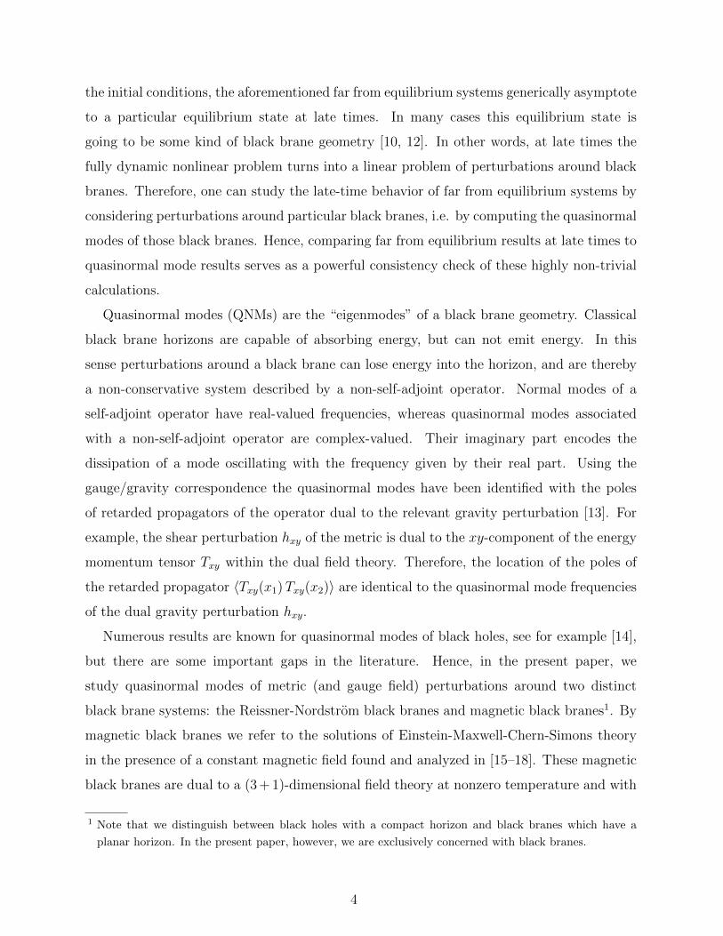
At increasing charge density and fixed momentum k = 0, the modes of set 1 move as

indicated in figure 4, displayed in the frequency ω. There is an obvious kink in the trajectories

at larger charge densities q ≈ 0.6qex. However, plotting the QNMs in the rescaled frequency

variable ω, no kinks are visible. Only upon multiplying ω with the horizon radius, those

kinks appear in the QNM trajectories. These kinks appear suspiciously close to the region

where convergence of the horizon expansion within our shooting method gets increasingly

worse.16 However, we have checked that the location of the kinks does not depend on the

numerical horizon and boundary cut-offs that we choose. Independently, the continued

fraction method confirms the kinks in the trajectories at the same locations. That said,

when plotting the frequencies in units of temperature (πT ), or in units of rH , we observe no

16 This is caused by fact that the inner horizon, located at r−, is approaching the outer horzion, located at

rH . The kink in the quasinormal mode trajectories appears where the difference |rH − r−| is comparable

to the horizon cut-off located at rcut−off , i.e. |rH − r−| ≈ |rH − rcut−off |.

27

q/qex ω (rescaled) ω/(πT )

0 ±3.11945− i2.74668 ±3.11945− i2.74668

0.1 ±3.11652− i2.75222 ±3.12256− i2.75756

0.2 ±3.10759− i2.76953 ±3.13227− i2.79153

0.3 ±3.09236− i2.80090 ±3.14994− i2.85305

0.4 ±3.07057− i2.85111 ±3.17859− i2.95141

0.5 ±3.04312− i2.92958 ±3.22533− i3.10499

0.6 ±3.01749− i3.05496 ±3.31032− i3.35142

0.7 ±3.03304− i3.25409 ±3.50619− i3.76173

0.8 ±3.16481− i3.47084 ±3.9918− i4.3778

0.9 ±3.32234− i3.68357 ±5.0231− i5.56924

TABLE II: Reissner-Nordstrom QNMs of hxy at q 6= 0, k = 0. Lowest QNM frequency in set 1

for increasing charge densities q (in units of (m/3)3/4) given in fractions of the extremal charge

density qex. The left column provides the QNM frequencies rescaled with a factor rH , while the

right column shows the frequencies of the same modes in units of (πT ).

kinks whatsoever, merely smooth trajectories. Hence, these kinks should be regarded as an

artifact of expressing frequencies in units of mass density. This point is explored in more

depth in one of the accompanying notebooks [33].

At vanishing momentum, k = 0, the leading QNM of the metric shear fluctuation hxy

is listed for increasing charge q of the Reissner-Nordstrom black brane in table II. The

right column shows the frequency values in units of (πT ), while the left column shows

the rescaled values which we obtain directly from our numerical procedure because therein

we have worked with conveniently rescaled quantities, as seen from the metric (7). Those

rescaled coordinates are convenient for our near-equilibrium setup. For a comparison to the

late-time behavior of physical quantities obtained from numerical non-equilibrium codes the

values in the right column are more suitable. In comparison with [19], our lowest QNM

values agree up to deviations of 0.2 percent, as can be seen from Table 1 in [19].

Fixing the momentum at larger values k = 1/2 and k = 1 does not change the qualitative

behavior of the modes, as seen from tables III and IV, respectively. Also in the quasinormal

mode trajectories computed at fixed nonzero momentum k = 1/2 we observe kinks, as

28

3 4 5 6 7

-8

-7

-6

-5

-4

-3

ReΩ

ImΩ

k=0

FIG. 4: Reissner-Nordstrom QNMs of hxy at q 6= 0, k = 0. The three trajectories of the three

lowest quasinormal modes are shown as the momentum is fixed to k = 0 and the charge is increased

from q = 0 to q = 0.9 qex in increments of ∆q = qex/40. The uppermost point in each trajectory

(top right point) corresponds to vanishing charge q = 0. For increasing charge, the modes each

move to more negative imaginary frequency values.

before at k = 0. See figure 5. However, at large fixed momentum, k = 5, we observe

that the kinks disappear from the regime accessible to our numerical methods, as seen

in figure 6. Another interesting exercise is to fix the charge density and then follow the

quasinormal modes while increasing the momentum. The result of this exercise can be seen

in figure 7 for fixed charges q = 0, 0.5qex, 0.8qex (blue, red, brown curves, respectively). At

large momentum, the trajectories all asymptote to the same “attractor” curve, regardless of

the charge. This seems reasonable because at large momentum the scale set by the charge

is negligible compared to the scale set by the momentum, in other words all trajectories at

large momentum should asymptote to the zero charge trajectory, which is confirmed by our

data.

Now we turn to the second set of quasinormal modes (set 2), namely the purely imaginary

ones mentioned before.17 The member of this set 2, which is closest to the origin ω = 0, is

17 We are grateful to Michal Heller for pointing us to these kinds of modes. Further, we are grateful to

Julian Sonner for discussions on the interpretation of these modes.

29

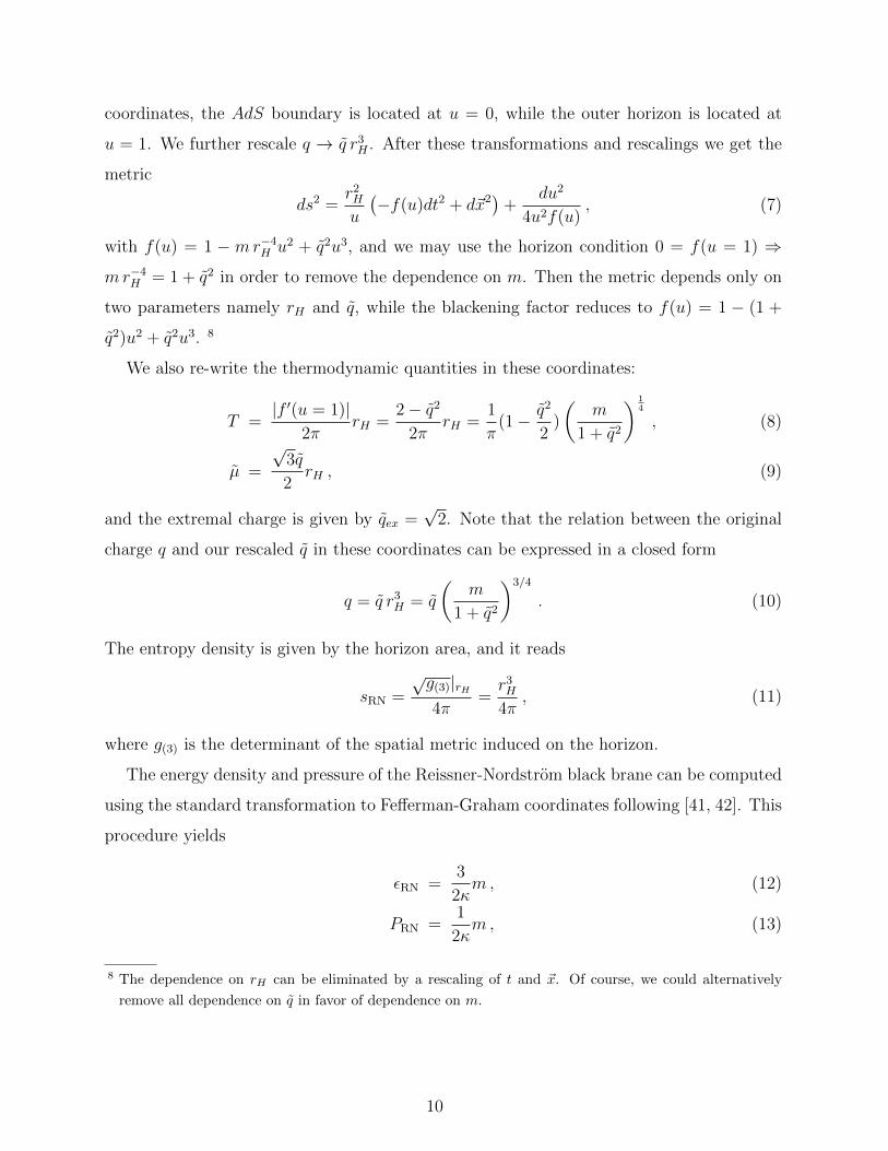
mode # 1 2 3

q = 0 ±3.1779741− i2.7290839 ±5.2112434− i4.7519066 ±7.2214147− i6.7604134

q = 0.25 qex ±3.1413918− i2.7474627 ±5.1413864− i4.7936400 ±7.1185609− i6.8281811

q = 0.5 qex ±3.0262710− i2.8281461 ±4.9367320− i4.9919741 ±6.8493201− i7.1646578

q = 0.75 qex ±2.9252877− i3.0924526 ±4.9163769− i5.3955189 ±6.8500839− i7.6457490

TABLE III: Nonzero momentum. Reissner-Nordstrom black brane quasinormal mode frequencies

ω for the tensor fluctuations, e.g. hxy, at fixed momentum k = 1/2 and increasing charge density

q.

mode # 1 2 3

q = 0 ±3.3440382− i2.6808260 ±5.3317107− i4.7178383 ±7.3188762− i6.7331804

q = 0.25 qex ±3.3102870− i2.6965339 ±5.2651313− i4.7562293 ±7.2195106− i6.7971758

q = 0.5 qex ±3.2045995− i2.7642384 ±5.0692976− i4.9339576 ±6.9544811− i7.1066419

q = 0.75 qex ±3.0864530− i2.9801352 ±5.0079788− i5.3207002 ±6.9204927− i7.5887749

TABLE IV: Nonzero momentum. Reissner-Nordstrom black brane quasinormal mode frequencies

ω for the tensor fluctuations, e.g. hxy, at fixed momentum k = 1 and increasing charge density q.

3 4 5 6 7-8

-7

-6

-5

-4

-3

ReΩ

ImΩ

k=1

FIG. 5: Reissner-Nordstrom QNMs of hxy at q 6= 0, k = 1. The trajectories of the three lowest

quasinormal modes are shown as the momentum is fixed to k = 1 and the charge is increased from

q = 0 to q = 0.9 qex in increments of ∆q = qex/40.

30

6 7 8 9

-7

-6

-5

-4

-3

ReΩ

ImΩ

k=5

FIG. 6: Reissner-Nordstrom QNMs of hxy at q 6= 0, k = 5. The trajectories of the three lowest

quasinormal modes are shown as the momentum is fixed to k = 5 and the charge is increased from

q = 0 to q = 0.9 qex in increments of ∆q = qex/40.

0 5 10 15 20

-3.0

-2.5

-2.0

-1.5

ReΩ

ImΩ

q=0, 0.5 qex, 0.8 qex

FIG. 7: The trajectory of the three lowest quasinormal modes are shown as the charge is fixed to

q = 0, 0.5 qex, or 0.8 qex while the momentum is increased from k = 0 to k = 20 in increments of

∆k = 0.1.

shown along with the lowest QNM from set 1 (and its complex conjugate) in figure 8. That

figure shows the trajectories of those three poles as the charge is increased from q = 0.6

to 1.0 in steps of 1/40. Note that we have chosen to display the rescaled frequencies here

31

(stemming from a rescaling of the time coordinate in the metric (7), as discussed before).18

While the lowest mode known from set 1 moves (slowly) away from the real axis, the lowest

mode of set 2 move on the negative imaginary axis towards the real axis. At a value of

qcrossing ≈ 0.655 the purely imaginary mode and the lowest mode of set 1 have identical

imaginary parts. See figure 9. At charge densities q > qcrossing ≈ 0.655, the lowest purely

imaginary mode is the lowest of all QNMs.

As the charge density approaches its extremal value from below, the modes of set 2 are

pushed towards the origin and closer towards each other. We conjecture that this may be

understood as the onset of a branch cut forming along the negative imaginary frequency

axis, in analogy to the near-extremal AdS4 case [51, 52].19 Our calculations indicate that

the modes of set 1 do not approach the imaginary axis in the extremal limit. All of the

QNMs of set 1 and set 2 remain in the lower half of the complex frequency plane. In other

words, the fluctuation hxy does not seem to cause any instabilities in the extremal limit (this

statement is limited by numerical accuracy).

We have confirmed selected QNMs of set 2 with the continued fraction method to an

accuracy of 4 digits.20 Various checks of both of our numerical methods indicate that these

purely imaginary modes of set 2 are a robust feature which is not an artifact of the numerical

methods. Consequently, the QNMs of set 2 are dominating the late-time physics of the

dual field theory at fairly sizable temperatures, namely at charges q > qcrossing ≈ 0.655,

corresponding to temperatures T < Tcrossing ≈ 0.228.

Our lowest tensor QNM frequency from set 1 agrees very well with the QNMs extracted

from the late-time behavior of the fully time dependent setup at the corresponding charge

densities. Table 1 in [19] shows a maximum deviation of 0.2% at fairly large charge densities.

At charge densities much smaller than the extremal one, we find much better agreement.

Note that Table 1 in [19] only probes charge densities for which the lowest QNM of set 1

18 We also find it convenient to express the charge density in its dimensionless form here, i.e. we are using

q as opposed to q.19 Just like in that case, at extremality, i.e. in the zero temperature limit, conformal symmetry is still broken

by the nonzero chemical potential.20 High accuracy at all parameter values is difficult to achieve in the purely imaginary QNMs. The problem

is that, at particular values of the charge q, the zeros of φ(u = 0, ω; q) move through poles of the function

φ(u = 0, ω; q). Those poles are located at ω = in(q2 − 2) (with integer n), where the continued fraction

method is known to yield false QNMs [1, 49].

32

ææ

òòòòòòòòòòòòòò

ò

ò

ò

òò

ææ

òòòòòòòòòòòòòòòò

ææ

òòòòòòòòòòòòòòòò

-4 -2 0 2 4

-4

-3

-2

-1

0

Re Ω

ImΩ

k=0

FIG. 8: At large charge densities, a purely imaginary QNM enters the low frequency regime.

We display the rescaled frequencies after ω → ω/rH . The trajectories of the three quasinormal

modes closest to the origin ω = 0 are shown as the charge increases from q = 0.6 to 1.0 in

increments of ∆q = 1/40. The momentum is fixed to k = 0. The black dots mark the points of

the respective trajectories with q = 0.6. The lowest QNM in set 1 and its complex conjugate mode

move downward as the charge increases (blue downward-pointing triangles). The lowest QNM in

set 2 moves upward as the charge increases (red upward-pointing triangles).

still dominates the late-time behavior. The authors of [19] use the charge density q which

takes its extremal value at√

2(m/3)3/4 ≈ 0.6204 with the mass parameter m = 1, while

the extremal charge value in the tilded coordinates is q =√

2. The relation between the

two charges is q = q(m/(1 + q2))3/4. Therefore, 90% of extremal charge in [19] is identical

to 58% of extremal charge in the tilded coordinates. The authors of [19] report numerical

difficulties with larger charge density values, whereas it is straightforward for us to reach

more than 70% of extremal charge in the tilded coordinates.

For comparison to [25], here we also compute the vector modes. The two lowest vector

QNMs (members of Set 1) at vanishing momentum ~k = 0 are given for various charges

in table V. Figure 10 shows their trajectories with increasing charge density, and we have

chosen the same units for our frequency as the authors of [25], i.e. we have plotted ω/(2πT ).

Note that the authors of [25] display results at nonzero momentum only, while all of our

vector QNM results are at vanishing momentum. Comparing to figure 1 from [25], we

33

0.60 0.65 0.70 0.75 0.80 0.85 0.90

-4

-3

-2

-1

0

q

ImΩ

k=0

FIG. 9: The imaginary part of the lowest QNM in set 1 is shown (line with negative slope) as

a function of charge q. This is compared to the imaginary part of the purely imaginary QNM

which is the lowest member of set 2 (line with positive slope). The two lines intersect at the charge

qcrossing ≈ 0.655 with an imaginary part of Imω ≈ −3.50.

observe qualitative agreement to the extent allowed by the visual comparison 21. We compare

to the left plot in figure 1 of [25]. In light of our own results, we interpret their green

data set (r−/r+ = 0.5) as similar to our vector QNMs at intermediate charge values, i.e.

roughly half of the extremal value of q. In that case, there is already one mode of Set 2

visible, sitting on the imaginary axis in their figure 1. We interpret their blue data set

(r−/r+ = 0.95) as showing only modes of Set 2 whereas the modes of Set 1 are outside

the plot range of their figure 1. Our numerical data at vanishing momentum does not

show the hydrodynamic (diffusion) mode closest to ω/(2πT ) = 0 indicated by the box in

figure 1 of [25]. At vanishing charge q = 0, we recover the values, ω/(2πT ) = n(±1 − i)

with n = 0, 1 , . . . , already obtained analytically in [53]. Just like for the tensor fluctuation,

also in this vector fluctuation a second set of purely imaginary QNM (Set 2) wanders up

the imaginary axis. And like the purely imaginary tensor QNMs, at a critical charge value

also these imaginary vector QNMs become more relevant to the late time behavior than the

21 The figure in [25] shows vector QNMs at nonzero spatial momentum. An analysis of the vector modes

at nonzero momentum is beyond the scope of this work, hence we content ourselves with a qualitative

comparison.

34

mode # q/qex = 0 q/qex = 0.8 q/qex = 0.9

Set 1 (complex QNMs)

1 ±1.0000000− i1.0000000 ±3.3687082− i1.5042378 ±6.3036022− i2.9733044

2 ±2.0000000− i2.0000000 ±5.8977388− i5.4108751 ±9.0680850− i6.1472415

Set 2 (purely imaginary QNMs)

1* not accessible ±0− i2.5337209 ±0− i2.3875204

2* not accessible ±0− i3.8897030 ±0− i3.4700708

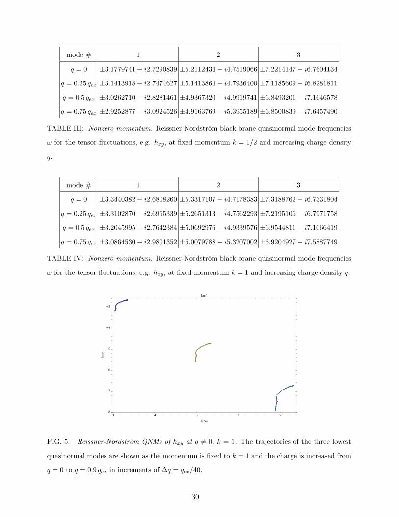
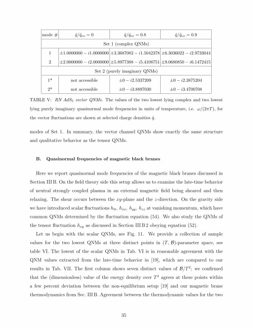
TABLE V: RN AdS5 vector QNMs. The values of the two lowest lying complex and two lowest

lying purely imaginary quasinormal mode frequencies in units of temperature, i.e. ω/(2πT ), for

the vector fluctuations are shown at selected charge densities q.

modes of Set 1. In summary, the vector channel QNMs show exactly the same structure

and qualitative behavior as the tensor QNMs.

B. Quasinormal frequencies of magnetic black branes

Here we report quasinormal mode frequencies of the magnetic black branes discussed in

Section III B. On the field theory side this setup allows us to examine the late-time behavior

of neutral strongly coupled plasma in an external magnetic field being sheared and then

relaxing. The shear occurs between the xy-plane and the z-direction. On the gravity side

we have introduced scalar fluctuations htt, hxx, hyy, hzz at vanishing momentum, which have

common QNMs determined by the fluctuation equation (54). We also study the QNMs of

the tensor fluctuation hxy as discussed in Section III B 2 obeying equation (52).

Let us begin with the scalar QNMs, see Fig. 11. We provide a collection of sample

values for the two lowest QNMs at three distinct points in (T, B)-parameter space, see

table VI. The lowest of the scalar QNMs in Tab. VI is in reasonable agreement with the

QNM values extracted from the late-time behavior in [19], which are compared to our

results in Tab. VII. The first column shows seven distinct values of B/T 2; we confirmed

that the (dimensionless) value of the energy density over T 4 agrees at these points within

a few percent deviation between the non-equilibrium setup [19] and our magnetic brane

thermodynamics from Sec. III B. Agreement between the thermodynamic values for the two

35

-5 0 5-6

-5

-4

-3

-2

-1

0

Re[ω/(2πT)]

Im[ω

/(2πT)]

FIG. 10: The two lowest complex and two lowest purely imaginary RN AdS5 vector QNM

frequencies in units of temperature, i.e. ω/(2πT ), are shown for increasing charge densities q/qex =

0.800, 0.805, 0.810, . . . , 0.895, 0.900. Like the tensor QNMs, also these vector QNMs fall into two

sets. Set 1 (blue down triangles) moves down in the complex plane as the charge density is increased.

Set 2 (red up triangles) moves up along the imaginary axis as charge density is increased. The

black dots mark the QNMs at q/qex = 0.800.

mode # B/T 2 = 0 B/T 2 = 12.953 B/T 2 = 30.161

1 ±3.1194506− i 2.7466751 ±3.4079677− i 3.0777933 ±3.8221728− i 3.5553514

2 ±5.1700747− i 4.7637826 ±5.4444069− i 5.5805876 ±5.6661971− i 6.6938458

TABLE VI: Magnetic brane scalar QNMs. The values of the two lowest lying quasinormal mode

frequencies ω for the scalar fluctuations, e.g. hxx − hzz, are shown in units of mass density. The

columns show the quasinormal mode frequencies for three distinct values of B/T 2. In the B → 0-

limit, these two modes connect smoothly to the two lowest modes of set 1 of the RN black brane

at vanishing charge density q = 0, i.e. to the ones found earlier by Starinets [1].

setups is best at small values of B/T 2 (about 0.2 percent) at point 2, then deviations rise

for bigger values, and asume their maximal value (about 2.3 percent) at point 7, i.e. for

relatively large B/T 2 = 30.161.

Now we turn to the tensor QNMs at vanishing momentum, two of which are shown in

Fig. 12. Note that the lowest tensor QNM approaches the imaginary frequency axis at

36

parameter point QNM late-time [19] relative deviation [in %]

ω ω ∆Reω, ∆Imω

1 (B/T 2 = 0.000) ±3.119450641− i 2.746675059 ±3.1195− i 2.7466 ±0.00002, −0.00003

2 (B/T 2 = 0.990) ±3.122662648− i 2.750477496 ±3.124− i 2.73 ±0.04283, −0.74451

3 (B/T 2 = 5.344) ±3.197822654− i 2.838566372 ±3.217− i 2.79 ±0.59970, −1.71095

4 (B/T 2 = 12.953) ±3.407967707− i 3.077793253 ±3.480− i 2.96 ±2.11364, −3.8272

5 (B/T 2 = 17.821) ±3.538016365− i 3.224040043 ±3.634− i 3.09 ±2.71292, −4.15752

6 (B/T 2 = 22.836) ±3.661199784− i 3.364602583 ±3.780− i 3.21 ±3.24484, −4.59497

7 (B/T 2 = 30.161) ±3.822172759− i 3.555351392 ±3.98− i3.38 ±4.12925,−4.93204

TABLE VII: Magnetic brane scalar QNMs versus far-from equilibrium late-time oscillations. The

value of the lowest lying quasinormal mode frequency ω for the scalar fluctuations, e.g. hxx − hzz,

are compared to the oscillation frequency extracted from the late-time behavior of the full time

evolution in [19].

0 1 2 3 4 5

-5

-4

-3

-2

-1

0

Re Ω

ImΩ

FIG. 11: Trajectories of the two lowest QNMs of scalar (hxx − hzz) fluctuations around magnetic

black branes: The magnetic field is increased from B/T 2 = 0 (at an energy density of ε/T 4 = 73.4)

to 15.5 (at an energy density of ε/T 4 = 147.6). These values are generated by fixing the near

horizon parameter u1 = 2, and choosing b = 0 to 19/20 in steps of ∆b = 1/20. Both, real and

imaginary part increase when the magnetic field (and with it the energy density) is increased. The

second QNM frequency moves a much greater distance in the complex frequency plane than the

first.

37

mode # B/T 2 = 5.342 B/T 2 = 22.80 B/T 2 = 30.00

1 ±3.0104279− i2.8338442 ±2.1829303− i3.4535515 ±1.8555798,−i3.7287196

2 ±4.9749665− i4.8923780 ±3.6619677− i5.3641251 ±3.6224530− i5.5936925

TABLE VIII: Magnetic brane tensor QNMs. The values of the two lowest lying quasinormal mode

frequencies ω for the tensor fluctuations, e.g. hxy, are shown in units of mass density. The columns

show the quasinormal mode frequencies for three distinct points in (T, B) parameter space. In the

B → 0-limit, these two modes connect smoothly to the two lowest modes of set 1 of the RN black

brane at vanishing charge density q = 0, i.e. to the ones found earlier by Starinets [1].

0 1 2 3 4 5

-10

-8

-6

-4

-2

0

Re ω

Imω

FIG. 12: QNMs of hxy fluctuations around magnetic black branes. The two lowest QNMs (both

members of set 1 in the limit of vanishing magnetic field, see Fig. 1) at vanishing momentum are

shown as the magnetic field parameter b is changed from b = 0 to b = 50/40 in steps of ∆b = 1/40.

These modes both move down and to the left with increasing b. This covers a magnetic field

over temperature range of B/T 2 = 0.0001, ..., 34.4555, which corresponds to energy densities of

ε/T 4 = 73.4, ..., 397.4. We have fixed the near horizon temperature parameter to u1 = 2.

large magnetic fields B 10. For the second QNM, however, our numerical results are

inconclusive at those large magnetic field values. We provide a collection of sample values

for the two lowest QNMs (from set 1) at three distinct points in (T, B)-parameter space in

Tab. VIII.

38

VI. CONCLUSION

Strongly coupled plasmas can be studied as they thermalize, because we have various

holographic methods at our disposal. What is the correct picture for such an evolution from

a ferocious state of matter to a tame thermal equilibrium? At late times in the thermalization

process, we at least have a fairly clear picture on the gravity side: just like the overtones

of a bell that was gently struck and then left to ring down freely, various quasinormal

modes (QNMs) of the black brane are excited. All but the lowest lying QNMs (with the

smallest imaginary part) have died down at late times because all but the lowest ones are

strongly damped. This picture is valid for small deviations from equilibrium and at late

times. However, one may be inclined to think of intermediate states, and possibly even the

initial state of the gravitational setup, as a superposition of (not necessarily quasinormal)

modes.22 23 Then, it would be interesting to know which of the modes are excited at what

time during the evolution, what energy they carry, and how quickly they dissipate. Is all

the energy first transferred from the low frequency modes into the high frequency modes, or

vice versa? Our analysis in comparison with the far from equilibrium data from [19] allows

a few speculations on which we comment below.

This present paper demonstrates the computation of tensor fluctuation (hxy) quasinor-

mal modes within two distinct black brane systems asymptoting to AdS5: First, Reissner-

Nordstrom (charged) black branes. Second, magnetic black branes (uncharged). In the

latter, we also compute the QNMs of scalar fluctuations htt, hxx, hyy, hzz, while in the

Reissner-Nordstrom case we re-compute the vector QNMs originally found in [25]. We pro-

vide sample values in tables I, II, III, IV, V, VI, VII,VIII. Two notebooks are provided

online [33] for computation of QNMs at user-selected charge density q and momentum kz,

or for reference QNM frequency values at particular magnetic fields B, and temperatures T .

All these quasinormal mode frequencies should be used in order to compare to holographic

22 A detailed analysis [54] found that a quasinormal mode decomposition approximates the full nonlinear

time evolution surprisingly well for all tested initial conditions. In order to support the idea of formulating

time-dependent systems in terms of a well-defined set of modes, we refer to the analysis of AdS5 black hole

QNMs performed in global AdS, and then reinterpreted in the Poincare patch [55]. There, the authors

relate that QNM spectrum to a time-dependent field theory stressing similarities to heavy ion collisions.23 Note also the perturbative weak field calculation of a gravitational collapse geometry in presence of

charge [56].

39

calculations of anisotropic fluids far from equilibrium. The late-time behavior of the latter

should be governed by oscillations and decay that is well approximated by particular QNMs.

As one example, we have compared our QNMs to a system [19] which starts with a metric

that is anisotropic between the xy-plane, and the z-direction, and which is then observed as

it freely evolves either in the presence of (i) charges or (ii) a magnetic field on the black brane.

We find good agreement. In the case of a charged plasma, dual to the Reissner-Nordstrom

AdS5 black brane (case (i)), our lowest tensor mode QNM (associated with fluctuations hxy

or equivalently hxx − hzz) agree with the values provided in [19] up to 0.2% deviation at

large charge densities.24 In the case of a magnetic plasma, dual to the magnetic AdS5 black

brane case (case (ii)), our lowest scalar QNM (associated with fluctuations hxx − hyy) is in

good (at worst 5% deviation) agreement with [19], see Tab. VI. These findings confirm our

reasoning from Section II, that the late-time behavior of a relaxing system is determined by

the symmetries of the background it relaxes towards, and by the symmetries of the initial

conditions. In the Reissner-Nordstrom case, the initial shear in the setup [19] (far from

equilibrium) is a tensor under SO(2) rotations in the xy-plane. At late times, only the

corresponding tensor QNM matters. In the magnetic black brane case, on the other hand,

the same initial shear is a scalar. At late times, only the corresponding scalar QNMs matter.

Furthermore, we provide QNM values for Reissner-Nordstrom black branes at nonzero

momentum. We may think of these QNMs as being useful for comparison to far from

equilibrium systems which started out with an initial condition depending on the z-direction.

Colliding shock waves with a z-dependent profile may serve as an example for this kind of

system.

At sizable charge densities, a novel set of QNMs dominates the late-time behavior of

the charged black brane system, and hence also the late-time behavior of the dual charged

plasma. In addition to the well known set of QNMs (set 1) of the Reissner-Nordstrom black

brane, we also found a set of purely imaginary QNMs (set 2) as schematically shown in

Fig. 1. These modes enter the low energy spectrum at and above a particular charge density

q ≥ 0.655, corresponding to a sizable temperature T ≤ Tcrossing ≈ 0.228, with the lowest

member of that set becoming the new lowest lying QNM of the sytem. As the sytem is

24 This may have to do with the lowest mode of set 2, beginning to play a significant role at these larger

densities; but not yet dominating the late-time behavior.

40

pushed toward extremality, based on our numerics, we conjecture that these modes of set 2

are going to be pushed towards each other and form a branch cut. An analogous behavior

is seen in the AdS4 case [51, 52].

In our second system, the magnetic black branes, we also find tensor QNMs at vanishing

momentum. We provide sample values in table VIII, and provide a notebook with samples

of QNMs at various temperatures, and magnetic fields.

It is interesting to note that all of the QNMs of magnetic branes move deeper into the

complex frequency plane as the magnetic field is increased. This should be interpreted as

a faster dissipation of each mode after it has been excited. It is then tempting to argue

for a faster equilibration of the non-equilibrium system if all the QNMs decay faster at

larger magnetic fields. However, this does not seem to be the case [19]. Instead, (charge

or) magnetic field individually seem to have a rather negligible effect on the equilibration

time [19]. This may be interpreted in (at least) two ways: as evidence for the fact that

(i) the standard QNMs (which we computed here) are not a good measure for equilibration

of this system while it is far from equilibrium, and one needs to find other ways of

characterizing this process, or

(ii) only the lowest of the QNMs plays a significant role in the equilibration process. This

is a possibility, because the lowest magnetic brane QNM remains virtually static,

while the higher magnetic brane QNMs change significantly with the magnetic field,

as illustrated in Fig. 11.

We point out a fundamentally different behavior for a subset of the electric black brane

QNMs. As noted in the previous paragraph for magnetic brane QNMs, most of the electric

brane QNMs move deeper into the complex plane at increasing charge density. The notewor-

thy exception are the QNMs of set 2, see Fig. 1. Those QNMs move closer to the origin of

the complex frequency plane while the charge is increased (and simultaneously temperature

approaches zero). 25 This behavior indicates a decreased dissipation of these modes, i.e.

these modes become more and more long-lived. It is tempting to ask if these modes become

25 Numerically, we can only verify this up to a certain lowest charge value, at which these imaginary QNMs

are simply too deep in the complex frequency for our methods to find them at the current accuracy.

However, all available results indicate that these imaginary QNMs move closer to ω = 0 with increasing

charge, at any given charge value.

41

part of an effective field theory description near zero temperature. Such a description could

contain these long-lived modes whose frequency is much smaller than the charge density,

i.e. ω q, near zero temperature. This would be in anology to the standard hydrodynamic

description of long-lived modes which satisfy the relation ω T . Such an effective field

theory description may be useful for the study of black holes near extremality. It should be

stressed that these modes are not propagating.

To provide a brief outlook, it would be interesting to consider the other fluctuations of our

two systems. All fluctuations could be studied at nonzero momentum in the z-direction. The

same can be done for a nonzero momentum in the y-direction. In that case, one would then

compute the QNMs of metric fluctuations which are vectors or scalars under the remaining

rotation group. Among those QNMs one expects diffusion and sound modes, i.e. modes

with dispersion relation ω ∝ k2 and ω ∝ k, respectively. This would then allow one to

compare to the late-time behavior of more complicated far from equilibrium systems.

Finally, we note that the shooting and continued fraction methods take quite a long

time to find the present results. More realistic, and thereby more complicated systems, do

encourage the development of improved methods for the computation of QNMs.

Acknowledgements

We thank J. Fuini, L. Yaffe for many helpful and inspiring discussions. We are grateful

to M. Heller and J. Sonner for discussions and for sharing some of their code. We thank

A. G. Green, A. Karch, W. van der Schee, and J. Zaanen for discussions. This work was

supported in part by the US Department of Energy under contract number de-sc0011637,

and in part by NSERC of Canada.

Appendix A: Generalization of Pincherle’s theorem and continued fraction method

In its generalization, Pincherle’s theorem relates m + 2 term recursion relations to m-

dimensional continued fractions. Such vectorial continued fractions require use of a pro-

jective space, all needed notions will be defined as they arise. The first useful result is

Parusnikov’s Theorem 2 which provides the correspondence

42

Theorem 2:

i) interuption-free m-dimensional continued fraction:

~f0 = ~b0 + a0~b1+

a1~b2+···

,

⇐⇒

iii) m+ 2 term recursion relation: gn =m+1∑j=1

pm+2−j,ngn−j,

where: ~pn ≡ (1/an, b1,n/an, · · · , bm,n/an); generically vi,j denotes the i-th component of

vector ~vj; and “interuption-free” means that an is non-zero.

The construction of the m-dimensional continued fraction is at first opaque, as it requires

“dividing by a vector,” but it can be simply accomplished by the following procedure. First,

given the vector ~pn, define

Pn ≡

0 · · · 0 p1,n

1 · · · 0 p2,n

.... . .

......

0 · · · 1 pm+1,n

, Qn = P0 · · ·Pn, J−1 ≡

0 1 0 · · · 0

0 0 1 · · · 0...

......

. . ....

0 0 0 · · · 1

1 0 0 · · · 0

. (A1)

These matrices act on m + 1-dimensional projective vectors, denoted (f1 : · · · : fm+1).

For the map σ−1 [(f1 : · · · : fm+1)] ≡ (f1/fm+1, · · · , fm/fm+1), the m-dimensional continued

fraction can be computed

~f0 ≡ limi→∞

~f(i)

0 ≡ limi→∞

σ−1J−1Qi~em+1, (A2)

where ~em+1 ≡ (0 : · · · : 0 : 1). Theorem 2 therefore provides a way to construct an m-

dimensional continued fraction given an m+ 2 term recursion relation.

The next theorem provides a powerful criterion for when the continued fraction ~f0 con-

verges.

Theorem 6:

An m-dimensional continued fraction ~f0 converges.

⇐⇒

There exists a minimal sequence hn that satisfies the recursion relation given in Theorem 2.

Parusnikov’s Theorems 7 and 8 now give a recursion relation that allows an explicit

determination of hn.

43

Theorem 7/8:

The minimal basis hn obeys:

hn =

(−1

fm,n+1

)hn−m +

m−1∑j=1

(−fj,n+1

fm,n+1

)hn−m+j , (A3)

where ~fn is the continued fraction ~fn ≡ ~bn + an/(~bn+1 + · · · ). This formula allows the

calculation of the quasinormal frequencies, as explicitly demonstrated in section IV B 2. By

setting n = m, the hi become the first m+1 coefficients of the recursion relation generated by

the equation of motion. One then uses (A2) to plug in the components of ~fm+1 as a function

of ω. Demanding the veracity of the formula in Theorem 7/8 determines the frequencies that

give the minimal solution, and hence are the quasinormal frequencies, as discussed above in

section IV B 1.

[1] A. O. Starinets, Phys.Rev. D66, 124013 (2002), hep-th/0207133.

[2] J. Adams et al. (STAR), Nucl.Phys. A757, 102 (2005), nucl-ex/0501009.

[3] K. Aamodt et al. (ALICE), Phys.Rev.Lett. 105, 252302 (2010), 1011.3914.

[4] T. W. B. Kibble, Journal of Physics A Mathematical General 9, 1387 (1976).

[5] W. H. Zurek, Nature (London) 317, 505 (1985).

[6] S. Mondal, D. Sen, and K. Sengupta, in Lecture Notes in Physics, Berlin Springer Verlag,

edited by A. K. K. Chandra, A. Das, and B. K. K. Chakrabarti (2010), vol. 802 of Lecture

Notes in Physics, Berlin Springer Verlag, p. 21, 0908.2922.

[7] P. M. Chesler and L. G. Yaffe, Phys.Rev.Lett. 106, 021601 (2011), 1011.3562.

[8] P. M. Chesler and L. G. Yaffe, Phys.Rev.Lett. 102, 211601 (2009), 0812.2053.

[9] P. M. Chesler and L. G. Yaffe, Phys.Rev. D82, 026006 (2010), 0906.4426.

[10] P. M. Chesler and L. G. Yaffe, JHEP 1407, 086 (2014), 1309.1439.

[11] J. M. Maldacena, Adv. Theor. Math. Phys. 2, 231 (1998), hep-th/9711200.

[12] S. Bhattacharyya, V. E. Hubeny, S. Minwalla, and M. Rangamani, JHEP 0802, 045 (2008),

0712.2456.

[13] P. K. Kovtun and A. O. Starinets, Phys.Rev. D72, 086009 (2005), hep-th/0506184.

[14] E. Berti, V. Cardoso, and A. O. Starinets, Class.Quant.Grav. 26, 163001 (2009), 0905.2975.

44

[15] E. D’Hoker and P. Kraus, JHEP 0910, 088 (2009), 0908.3875.

[16] E. D’Hoker and P. Kraus, JHEP 1003, 095 (2010), 0911.4518.

[17] E. D’Hoker and P. Kraus, JHEP 1005, 083 (2010), 1003.1302.

[18] E. D’Hoker and P. Kraus, Class.Quant.Grav. 27, 215022 (2010), 1006.2573.

[19] J. F. Fuini and L. G. Yaffe (2015), 1503.07148.

[20] R. A. Konoplya and A. Zhidenko, Rev. Mod. Phys. 83, 793 (2011), URL http://link.aps.

org/doi/10.1103/RevModPhys.83.793.

[21] E. Berti and K. Kokkotas, Phys. Rev. D 67, 064020 (2003), URL http://link.aps.org/

doi/10.1103/PhysRevD.67.064020.

[22] H. Kodama and A. Ishibashi, Prog.Theor.Phys. 111, 29 (2004), hep-th/0308128.

[23] R. Konoplya and A. Zhidenko, Phys.Rev. D78, 104017 (2008), 0809.2048.

[24] H. Kodama and A. Ishibashi, Prog.Theor.Phys. 110, 701 (2003), hep-th/0305147.

[25] K. Maeda, M. Natsuume, and T. Okamura, Phys.Rev. D73, 066013 (2006), hep-th/0602010.

[26] J. Natario and R. Schiappa, Adv.Theor.Math.Phys. 8, 1001 (2004), hep-th/0411267.

[27] J. Mas, JHEP 03, 016 (2006), hep-th/0601144.

[28] D. T. Son and A. O. Starinets, JHEP 0603, 052 (2006), hep-th/0601157.

[29] Y. Matsuo, S.-J. Sin, S. Takeuchi, T. Tsukioka, and C.-M. Yoo, Nucl. Phys. B820, 593 (2009),

0901.0610.

[30] X.-H. Ge, Y. Matsuo, F.-W. Shu, S.-J. Sin, and T. Tsukioka, Prog. Theor. Phys. 120, 833

(2008), 0806.4460.

[31] Y. Matsuo, S.-J. Sin, S. Takeuchi, and T. Tsukioka, JHEP 04, 071 (2010), 0910.3722.

[32] Wolfram Research, Inc. Version 9.0 (2012).

[33] S. Janiszewski and M. Kaminski, Mathematica notebooks for computation of tensor

(nonzero momentum) and vector (zero momentum) quasinormal modes of Reissner-Nordstrom

black holes at user-selected charge density, as well as scalar and tensor quasinormal

mode equations for the magnetic brane case; see ‘ancillary files’ on arXiv. (2015),

www.arxiv.org/abs/1508.06993 [Ancillary Files].

[34] A. S. Miranda, J. Morgan, and V. T. Zanchin, JHEP 11, 030 (2008), 0809.0297.

[35] M. Bhaseen, J. P. Gauntlett, B. Simons, J. Sonner, and T. Wiseman, Phys.Rev.Lett. 110,

015301 (2013), 1207.4194.

[36] A. Buchel, M. P. Heller, and R. C. Myers (2015), 1503.07114.

45

[37] G. Policastro, D. Son, and A. Starinets, Phys.Rev.Lett. 87, 081601 (2001), hep-th/0104066.

[38] P. Kovtun, D. T. Son, and A. O. Starinets, JHEP 0310, 064 (2003), hep-th/0309213.

[39] P. Kovtun, D. Son, and A. Starinets, Phys.Rev.Lett. 94, 111601 (2005), an Essay submitted

to 2004 Gravity Research Foundation competition, hep-th/0405231.

[40] G. Policastro, D. T. Son, and A. O. Starinets, JHEP 0209, 043 (2002), hep-th/0205052.

[41] S. de Haro, S. N. Solodukhin, and K. Skenderis, Commun.Math.Phys. 217, 595 (2001), hep-

th/0002230.

[42] K. Skenderis, Class.Quant.Grav. 19, 5849 (2002), hep-th/0209067.

[43] C. Fefferman and C. R. Graham, Asterisque pp. 95–116 (1985), ISSN 0303-1179, the mathe-

matical heritage of Elie Cartan (Lyon, 1984).

[44] A. Petkou and K. Skenderis, Nucl.Phys. B561, 100 (1999), hep-th/9906030.

[45] M. Kaminski, K. Landsteiner, F. Pena-Benitez, J. Erdmenger, C. Greubel, et al., JHEP 1003,

117 (2010), 0911.3544.

[46] M. Kaminski, Fortsch.Phys. 57, 3 (2009), 0808.1114.

[47] I. Amado, M. Kaminski, and K. Landsteiner, JHEP 05, 021 (2009), 0903.2209.

[48] M. Kaminski, K. Landsteiner, J. Mas, J. P. Shock, and J. Tarrio, JHEP 1002, 021 (2010),

0911.3610.

[49] S. Janiszewski, JHEP 1209, 093 (2012), 1112.0085.

[50] V. Parusnikov, Mathematical Notes 78, 827 (2005), ISSN 0001-4346, URL http://dx.doi.

org/10.1007/s11006-005-0188-7.

[51] M. Edalati, J. I. Jottar, and R. G. Leigh, JHEP 1004, 075 (2010), 1001.0779.

[52] M. Edalati, J. I. Jottar, and R. G. Leigh, JHEP 1010, 058 (2010), 1005.4075.

[53] A. Nunez and A. O. Starinets, Phys. Rev. D67, 124013 (2003), hep-th/0302026.

[54] M. P. Heller, D. Mateos, W. van der Schee, and M. Triana, JHEP 09, 026 (2013), 1304.5172.

[55] J. J. Friess, S. S. Gubser, G. Michalogiorgakis, and S. S. Pufu, JHEP 0704, 080 (2007),

hep-th/0611005.

[56] E. Caceres, A. Kundu, J. F. Pedraza, and D.-L. Yang, JHEP 06, 111 (2015), 1411.1744.

46