Department of Pesticide Regulation · HSG assignments to different soils ... measured by the Department of Pesticide Regulation in a variety of soil ... but the majority are based

Department of Pesticide Regulation

Mary-Ann Warmerdam Director M E M O R A N D U M

Arnold Schwarzenegger Governor

1001 I Street • P.O. Box 4015 • Sacramento, California 95812-4015 • www.cdpr.ca.gov A Department of the California Environmental Protection Agency

TO: John S. Sanders, Ph.D., Chief Environmental Monitoring Branch FROM: Frank Spurlock, Ph.D. [Original signed by Frank Spurlock] Senior Environmental Research Scientist Environmental Monitoring Branch (916) 324-4124 DATE: November 9, 2004 SUBJECT: WORK PLAN FOR DEVELOPMENT OF AN EMPIRICAL SURFACE

WATER RUNOFF INDEX FROM FIELD-MEASURED INFILTRATION DATA

Summary This memorandum describes a general work plan for developing a surface water runoff index for soils from field-measured infiltration rates (infiltrabilities). Several studies will be needed to develop and validate the index. The general goal is to describe the relative runoff potential of different soil types under different seasonal and agricultural management conditions. A runoff index may be used in conjunction with pesticide use data to (1) identify soils or regions that contribute disproportionately to pesticide runoff, (2) focus outreach, education, and management practice implementation efforts to obtain the most benefit for the cost, and/or (3) efficiently target surface water sampling in monitoring studies. A detailed discussion of some technical and experimental considerations is provided in the attachment. Introduction Dormant, in-season insecticides, and a variety of preemergent herbicides have been detected in California surface water runoff. The tendency of a pesticide to move off-site in runoff depends on several factors, including location and timing of use relative to storm or irrigation events, pesticide properties, and soil properties. California�s agricultural soils range from coarse sands to fine clays and so display a range of hydraulic characteristics. Coarse soils are often highly permeable while finer-textured soils are usually more prone to runoff. Because the hydraulic characteristics of soils are so variable, different regions (with different soils) contribute disproportionately to both surface water runoff and pesticide runoff. Currently, the most common method of describing a soil�s runoff tendencies is to use an assigned parameter called �hydrologic soil group� (HSG). However, HSG assignments to different soils are, apparently, inconsistent and subjective (see attached).

John S. Sanders November 9, 2004 Page 2

Furthermore, HSG assignments are based on native soil characteristics; they do not account for the effect of agronomic management practices on soil runoff tendencies. Consequently, HSGs are probably only qualitative indicators of runoff potential and are therefore, of limited practical value. This work plan proposes development and validation of a runoff index using infiltration data measured by the Department of Pesticide Regulation in a variety of soil types, in different seasons, and under different agricultural management conditions. Work will initially focus on Central Valley soils where orchard crops are grown because these are currently important sources of pesticides in runoff. Future work may include extension to other cropping systems under both rain and irrigation runoff conditions. The infiltration data will be used to develop a general predictive model to estimate soil infiltrabilities from soil physical characteristics and site-specific agricultural management practices. HSGs may be included in the model as a predictor variable. Following model development, validation studies will be conducted to (1) compare the accuracy of the infiltrabilities predicted by the model, and (2) relate those infiltrabilities to actual runoff behavior in small plots. Objective The objective of this work plan is to develop and validate an empirical soil runoff index based on measured infiltration data, soil properties, and site-specific agricultural management practices. The index will be a measure of a soil�s relative tendency to yield runoff from irrigation or rainfall conditions. General work plan outline Work will initially focus on soils where orchard crops are grown because these are currently important sources of pesticides in runoff. The work plan will consist of the following general steps: A. Identify orchard soils in the Sacramento and San Joaquin Valleys. B. Collect infiltration data for a subset of orchard soils. At minimum, ancillary data will

include surface bulk density, moisture content, surface soil sample, irrigation water source, and general orchard floor management practices. Characterize repeatability of the infiltration measurement method, within field spatial variability, and seasonal variability of soil infiltrabilities.


C. Compare measured infiltrabilities to soil survey infiltration estimates and HSG classifications. Develop a mathematical model relating measured infiltrabilities to soil properties and agricultural management practices.

D. Use the model to predict infiltrabilities on the remainder of orchard soils in the Sacramento and San Joaquin Valleys.

E. First stage validation: measure infiltrabilities on a subset of the soils in D above. Compare measured results to model predicted infiltrabilities to validate predictions.

F. Second stage validation: conduct small plot water/bromide runoff studies to compare the extent of runoff as a function of predicted infiltrabilities for same soils used in e above.

An initial pilot study has begun (Gill, 2004) that includes step A on previous page and will begin to provide data for steps B and C. The outline above represents an extended work plan and model development may take two to three years depending on staff resources and time available for field work. Completion of the validation studies may take an additional two years, subject to the same resource constraints. A more detailed time line for this project will be developed after data from preliminary studies are analyzed to provide general estimates of within-field variation, within-soil group variation, and seasonal variation in infiltrabilities. Attachment bcc: Spurlock Surname File


Reference: Gill, S. 2004. Study 223: Protocol to Determine the Effect of Cover Crop and Filter Strip Vegetation on Reducing Pesticide Runoff to Surface Water. Phase 1: Pilot Study and Method Development. Environmental Monitoring Branch, Department of Pesticide Regulation. Available on-line at <http//www.cdpr.ca.gov/docs/empm/pubs/protocol.htm.

Attachment 1 � 11/18/04 page 1

1

ATTACHMENT 1

This attachment provides background information on Hydrologic Soil Groups

(HSG), infiltration, and discusses potential problems and approaches to

developing an empirically-based runoff index from measured infiltration data.

A. Hydrologic Soil Groups Soil runoff tendencies are most commonly described by their �hydrologic soil

group� (HSG) classification. HSGs are used to determine a soil�s runoff �curve

number�, a parameter widely used in surface water runoff models for partitioning

precipitation or irrigation inputs between runoff and infiltration. The four principal

hydrologic soil groups (HSG) are defined as follows (USDA-NRCS, 1986):

Group A. (Low runoff potential). Soils having high infiltration

rates even when thoroughly wetted and consisting chiefly of

deep, well to excessively drained sands or gravels. These soils

have a high rate of water transmission.

Group B. Soils having moderate infiltration rates when thoroughly

wetted and consisting chiefly of moderately deep to deep, moderately

well to well drained soils with moderately fine to moderately

coarse textures. These soils have a moderate rate of water transmission.

Group C. Soils having slow infiltration rates when thoroughly wetted

and consisting chiefly of soils with a layer that impedes downward

movement of water, or soils with moderately fine to fine texture.

These soils have a slow rate of water transmission.

Group D. (High runoff potential). Soils having very slow infiltration

rates when thoroughly wetted and consisting chiefly of clay soils

with a high swelling potential, soils with a permanent high water


2

table, soils with a claypan or clay layer at or near the surface,

and shallow soils over nearly impervious material. These soils

have a very slow rate of water transmission.

DPR has HSG data for California soils obtained from soil surveys. Originally,

HSG assignments �were based on the use of rainfall-runoff data from small

watersheds or infiltrometer plots, but the majority are based on the judgments of

soil scientists and correlators who used physical properties of the soil in making

their decisions� (Mockus, 1972). The HSG assignments for different soils are

therefore subjective, and the reliability of these assignments have been

questioned. For example, USDA National Soil Survey scientists state:

�Assignment of soils to hydrologic soils groups has been based on published

criteria subjectively interpreted and applied by soil scientists. As a results,

hydrologic soil group placement for any given soil lacks consistency of method

and correlation to the respective soil�s physical properties.� (Nielsen and

Hjelmfelt ,1998). Further, HSGs do not consider other factors such as orchard

floor management practices or vegetative conditions.

B. About infiltration Infiltrability is the preferred soil physics terminology for infiltration rate (Hillel,

1980). Surface water runoff occurs when the rate of precipitation exceeds

infiltrability. Consequently, soils with high infiltrabilities have a lesser runoff

potential than those with low infiltrabilities. An approximation for infiltration in

homogeneous soils is

AtStI += 5.0

where I is cumulative infiltration (l), S is the sorptivity (l/t)1/2, t is time, and A (l t-1)

is a soil parameter that is comparable to a soil�s saturated hydraulic conductivity

(Hillel, 1980). Infiltrability (l/t) at any time during the runoff process is then given

by:


3

AStdtdI += − 5.0

The numerical value of the sorptivity S is typically much greater than A (Taylor

and Ashcroft, 1972), so that the first term dominates early in the infiltration

process, but at very large times becomes insignificant relative to the second

term. Consequently S reflects the initial infiltrability, and A reflects steady-state

infiltrability that occurs at later times.

As a first-cut approximation, a runoff index �R� might be assumed equal to A, the

steady state infiltrability. If this is the case, large values of R will denote low

runoff tendency while small values will indicate a high runoff potential.

Alternately, a meaningful R may be some function of both A and S: R = R(S,A).

The final choice of R(S,A) will probably depend on comparison of a large body of

actual infiltration data to �characteristic� storm durations. The latter might be

determined from statistical analysis of hourly rainfall data from different areas of

the Central Valley.

B1. Measuring S and A

Gill (2004) conducted background literature research on methods for measuring

infiltrability in the field, concluding that the recently introduced Cornell sprinkler

infiltrometer holds promise as an inexpensive, convenient and rapid

measurement tool (Ogden et al., 1997). A DPR study has commenced with the

general objective of field testing this infiltrometer and developing field infiltrability

measurement procedures, including estimates of expected spatial and temporal

infiltration variability in common orchard soils (Gill, 2004). The measurement

method allows measurement of sorptivity S and the steady state infiltrability A.


4

C. Example of runoff index development This section provides an illustrative example of runoff index development. The

purpose of this example is to:

��outline one possible procedure,

��illustrate potential difficulties and considerations, and

��foster additional discussion and thinking.

The workplan proposes development of a predictive model that relates a runoff

index R (the response variable) to various predictor variables such as soil

physical properties (e.g., texture, presence of a hardpan layer, etc.). As

discussed earlier, R will be calculated as some function R(S,A) when such

measured data are available. A training set will be used to develop a model

relating R to predictor variables. The model could then be used to predict R from

easily obtained predictor variables (e.g., from soil survey data) for other areas or

soils for which measured infiltration data are not available.

Because there are no extensive infiltration datasets available, the illustrative example here uses sectional estimates of HSG as a response variable, essentially serving as a surrogate for a measured runoff index (infiltrabilities).

C1. Response variable - HSG

The HSG data used as the response variable in this example were obtained as

sectional estimates developed from soil survey data. The sectional estimates

were developed by numerically coding the hydrologic soil group classifications for

each soil (e.g., A=0, B=2, etc.) and averaging all codes for each soil that

occurred in a section (Troiano et al., 2000). There was no weighting performed

for relative abundance of soil types present in each section. The sectional HSG

estimate is given the name hyd. Hyd is bounded: the maximum value is 6 (all

soils in a section belong to HSG �D�) and the minimum value is 0 (all soils in a

section belong to HSG �A�).


5

C2. Predictor variables

Examples of soil physical properties that are related to the runoff tendency of a

soil � and therefore hyd - include textural composition (percent clay, sand), bulk

density, permeability, water-holding capacity, the presence of a hard pan, and

the presence of a shallow seasonal water-table. Based on knowledge of soil

properties that influence runoff potential, a model to predict the response variable

hyd will require including most, if not all, of the foregoing predictor properties.

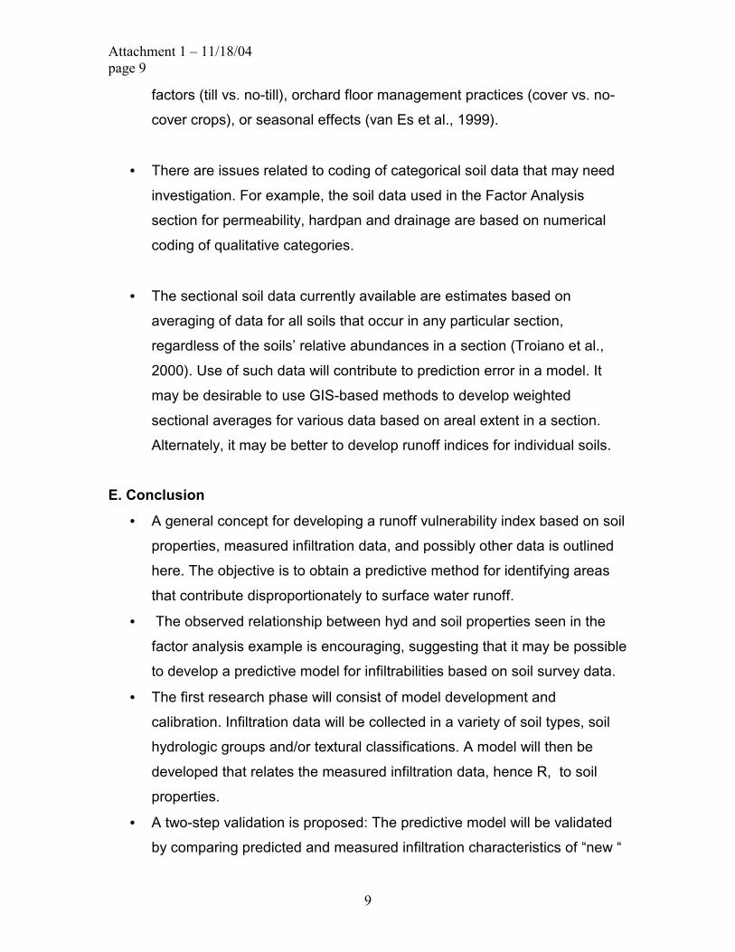
Estimates for the predictor variable data are available from soil surveys, but the

variables are highly collinear (e.g. Figure 1, Table 1). Because the variables are

not independent, conventional regression methods are of limited usefulness for

developing a model relating HSG to soil properties.

C3. Factor analysis

Factor analysis is one method for reducing the dimensionality of a data set,

where new orthogonal transformed variables are derived from linear

combinations of the original variables. While there are some general similarities

between Principle Component Analysis and Factor Analysis, one advantage of

the latter is that the new variables, or factors, can often be interpreted

meaningfully. This is not typically the case with principal components.

Table 2 is an example of Factor Analysis of sectional percent silt, percent sand,

AWC (available water capacity), Permeability, Hardpan, Drainage and Water

Table soil data for approximately 16,500 sections in California�s Central Valley.

The analysis was performed on the correlation matrix because of the different

measurement scales of the variables. As an aside, a goal of the actual research

project is to develop a mathematical model based on new (uncorrelated) factors

for predicting infiltrabilities. It�s critical to recognize that the actual soil variables

selected for factor analysis in that case will be selected based on a priori

knowledge of the infiltration process. Eventual development of such a model


6

may include the seven variables listed above, additional soil or management

variables, or additional data from other sources.

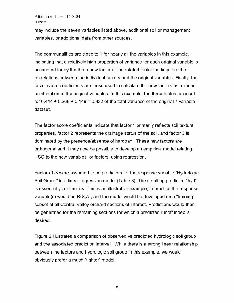
The communalities are close to 1 for nearly all the variables in this example,

indicating that a relatively high proportion of variance for each original variable is

accounted for by the three new factors. The rotated factor loadings are the

correlations between the individual factors and the original variables. Finally, the

factor score coefficients are those used to calculate the new factors as a linear

combination of the original variables. In this example, the three factors account

for 0.414 + 0.269 + 0.149 = 0.832 of the total variance of the original 7 variable

dataset.

The factor score coefficients indicate that factor 1 primarily reflects soil textural

properties, factor 2 represents the drainage status of the soil, and factor 3 is

dominated by the presence/absence of hardpan. These new factors are

orthogonal and it may now be possible to develop an empirical model relating

HSG to the new variables, or factors, using regression.

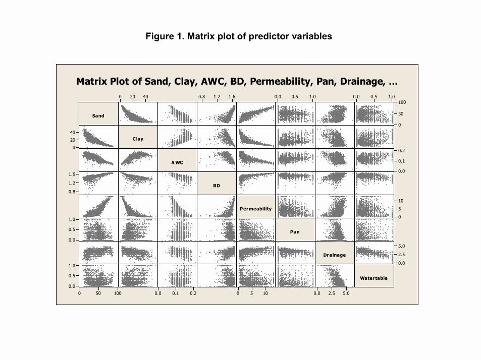
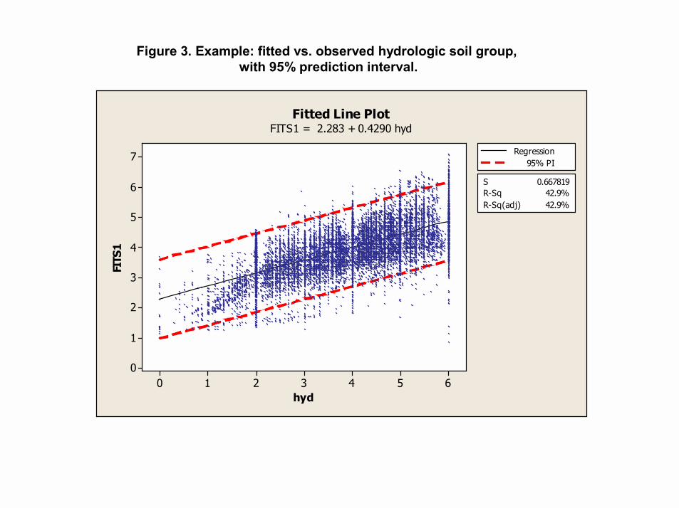
Factors 1-3 were assumed to be predictors for the response variable �Hydrologic

Soil Group� in a linear regression model (Table 3). The resulting predicted �hyd�

is essentially continuous. This is an illustrative example; in practice the response

variable(s) would be R(S,A), and the model would be developed on a �training�

subset of all Central Valley orchard sections of interest. Predictions would then

be generated for the remaining sections for which a predicted runoff index is

desired.

Figure 2 illustrates a comparison of observed vs predicted hydrologic soil group

and the associated prediction interval. While there is a strong linear relationship

between the factors and hydrologic soil group in this example, we would

obviously prefer a much �tighter� model.


7

The regression diagnostic plot illustrates a problem that arises when using

bounded data (Figure 3). There is a corresponding sharp upper and lower bound

for the residuals that varies with the fit. In practice, a transformation or alternate

analysis may be required for this particular case. The measured infiltration data

should not have this problem.

The prediction limits are relatively wide (Figure 2). Several potential reasons

include: (a) errors in the response data (e.g., inconsistency in HSG assignments

discussed earlier), (b) the use of sectional estimates for all soil variables �

including HSG - instead of data for individual soil types, (c) the actual �best�

relationship between predictors and response variable may be nonlinear, and/or

(d) the model may not account for all factors that influence hyd.

Figure 4 completes this example, illustrating a runoff tendency plot based on the

predicted hyd (soil hydrologic group data). The qualitative classifications of

runoff potential in the legend of low, moderate, etc., are based on the hydrologic

soil group definitions.

In practice, a two-stage validation study will be conducted to (a) test the veracity

of the predicted Rs, and (b) characterize the relationship between small-plot

runoff behavior and the predicted Rs.

C4. Other approaches

Other approaches for developing a predictive relationship between infiltrability

data and soil physical properties are possible. These should be investigated. Two

of these are:

1. Partial least squares regression (PLS). PLS is a general regression method

useful for situations where predictor variables are collinear, and is effective for

reducing the number of predictor variables (Geladi and Kowalski, 1985).. It may

be suitable for the soil data discussed here.


8

2. Simple calibration/correction of existing hydrologic soil group assignments

using measured infiltration data as mentioned earlier. This option has the benefit

of being less complex than the multivariate approaches. One disadvantage is

that four runoff tendency categories may not provide enough resolution to be as

useful as a continuous variable.

The approach taken will ultimately depend on (a) the variability of infiltration data

within and between soil types, (b) the effect of soil management practices on

infiltration rates, and (c) the strength of the putative relationship between

measured infiltration data and soil physical properties (texture, presence of

hardpan, presence of a seasonal water table, etc.).

D. Potential difficulties/additional considerations. Some of these include:

• The spatial and temporal variability associated with field infiltrabilties may

prevent development of a quantitative runoff index. If this is the case, the

approach mentioned under 2, above, may be the most appropriate.

• The form of the Runoff index R that best represents a soil�s runoff

tendency is unclear. Sorptivity S may need to be combined algebraically

with A, or 2 separate response variables (S and A) may be required.

Alternately, A alone may be sufficient. An answer to this question may

become evident after analysis of infiltrability data from several soils.

• While there should be a relationship between soil factors and infiltration,

the error in such a relation may be substantial. Additional data will

probably need to be incorporated into the model. Such data may include

the field-measured surface bulk density, water content, soil management


9

factors (till vs. no-till), orchard floor management practices (cover vs. no-

cover crops), or seasonal effects (van Es et al., 1999).

• There are issues related to coding of categorical soil data that may need

investigation. For example, the soil data used in the Factor Analysis

section for permeability, hardpan and drainage are based on numerical

coding of qualitative categories.

• The sectional soil data currently available are estimates based on

averaging of data for all soils that occur in any particular section,

regardless of the soils� relative abundances in a section (Troiano et al.,

2000). Use of such data will contribute to prediction error in a model. It

may be desirable to use GIS-based methods to develop weighted

sectional averages for various data based on areal extent in a section.

Alternately, it may be better to develop runoff indices for individual soils.

E. Conclusion

• A general concept for developing a runoff vulnerability index based on soil

properties, measured infiltration data, and possibly other data is outlined

here. The objective is to obtain a predictive method for identifying areas

that contribute disproportionately to surface water runoff.

• The observed relationship between hyd and soil properties seen in the

factor analysis example is encouraging, suggesting that it may be possible

to develop a predictive model for infiltrabilities based on soil survey data.

• The first research phase will consist of model development and

calibration. Infiltration data will be collected in a variety of soil types, soil

hydrologic groups and/or textural classifications. A model will then be

developed that relates the measured infiltration data, hence R, to soil

properties.

• A two-step validation is proposed: The predictive model will be validated

by comparing predicted and measured infiltration characteristics of �new �


10

(previously untested) soils. Small-plot bromide runoff experiments will then

be conducted to compare the infiltration characteristics of different soils to

actual runoff behavior.

• Initial attempts at developing these runoff indices should be restricted to

orchard crop land use so that the variability arising from the effect of

diverse cropping management practices is reduced.

• Several considerations or potential difficulties in data treatment and

model development are likely to arise.

• This project may take several years of data acquisition and analysis.


11

F. References

Geladi, P. and B.R. Kowalski. 1985. Partial least-squares regression: a tutorial. Analytica Chimica Acta, 185:1-17.

Gill, S. 2004. Study 223: Protocol to determine the effect of cover crop and filter

strip vegetation on reducing pesticide runoff to surface water. EM Branch, DPR.

Hillel, D. 1980. Applications of Soil Physics. Academic Press, NY.

Mockus, V. 1972. Hydrologic Soil Groups. Chapter 7, Section 4, SCS National

Engineering Handbook. Nielsen, R. D. and A. T. Hjelmfelt. 1998. Hydrologic soil group assessment.

Water Resources Engineering 98. IN: Abt, Young-Pezeshk and Watson (eds.), Proc. of International Water Resources Eng. Conf., Am. Soc. Civil Engr:1297-1302.

Ogden, C.B., H.M. van Es, and R.R. Schindelbeck. 1997. Miniature rain simulator

for field measurement of soil infiltration. Soil Sci. Soc. Am. Proc., 61:1041-1043.

Taylor, S.A., and G.L. Ashcroft. 1972. Physical Edaphology: the physics of

irrigated and nonirrigated soils. W. Freeman and Co., San Francisco.

Troiano, J., F. Spurlock, and J. Marade. 2000. Update of the California vulnerability soil analysis for movement of pesticides to ground water: Report EH 00-05.

Van es, H.M., C.B. Ogden, R.L. Hill, R.R. Schindlebeck, and T. Tsegaye. 1999.

Integrated assessment of space, time, and management related variability of soil hydraulic properties. Soil Sci. Soc. Am. J., 63:1599-1608.

Table1. Correlation matrix for selected soil properties.

Correlations: Sand, Silt, Clay, AWC, Permeability, Pan, Drainage, Watertable

Sand Silt Clay AWC Permeability Pan DrainageSilt -0.582

0.000

Clay -0.766 0.5470.000 0.000

AWC -0.575 0.748 0.5920.000 0.000 0.000

Permeability 0.723 -0.538 -0.671 -0.5270.000 0.000 0.000 0.000

Pan 0.091 -0.134 0.032 -0.090 -0.1010.000 0.000 0.000 0.000 0.000

Drainage 0.283 -0.428 -0.498 -0.343 0.223 -0.0320.000 0.000 0.000 0.000 0.000 0.000

Watertable -0.224 0.281 0.392 0.211 -0.072 -0.054 -0.7680.000 0.000 0.000 0.000 0.000 0.000 0.000

Cell Contents: Pearson correlationP-Value

Table 2. EXAMPLE: Principal Component Factor Analysis ofthe Correlation Matrix

Rotated Factor Loadings and CommunalitiesVarimax Rotation

Variable Factor1 Factor2 Factor3 Communalitysand 0.896 0.115 0.088 0.823clay -0.830 -0.366 0.058 0.826awc -0.749 -0.184 -0.145 0.617perm 0.884 -0.025 -0.163 0.809pan 0.015 0.001 0.990 0.980drain 0.235 0.907 -0.054 0.880wattab -0.085 -0.939 -0.059 0.892

Variance 2.8967 1.8856 1.0446 5.8269% Var 0.414 0.269 0.149 0.832

Factor Score Coefficients

Variable Factor1 Factor2 Factor3sand 0.333 -0.084 0.086clay -0.264 -0.081 0.058awc -0.264 0.019 -0.139perm 0.351 -0.163 -0.153pan 0.009 -0.017 0.948drain -0.062 0.509 -0.065wattab 0.126 -0.552 -0.043

Table 3. Regression Analysis: hyd versus score1, score2, score3 The regression equation ishyd = 4.00 - 0.687 score1 - 0.382 score2 + 0.404 score3

Predictor Coef SE Coef T PConstant 3.99768 0.00793 504.20 0.000score1 -0.687086 0.007929 -86.66 0.000score2 -0.381847 0.007929 -48.16 0.000score3 0.403919 0.007929 50.94 0.000

S = 1.01963 R-Sq = 42.9% R-Sq(adj) = 42.9%

PRESS = 17198.5 R-Sq(pred) = 42.87%

Analysis of Variance

Source DF SS MS F PRegression 3 12916.2 4305.4 4141.21 0.000Residual Error 16534 17189.5 1.0Total 16537 30105.6

Sand

40200 1.61.20.8 1.00.50.0 1.00.50.0100

50

0

40

20

0

Clay

A WC

0.2

0.1

0.01.6

1.2

0.8BD

Permeability

10

5

01.0

0.5

0.0

Pan

Drainage

5.0

2.5

0.0

100500

1.0

0.5

0.00.20.10.0 1050 5.02.50.0

Watertable

Matrix Plot of Sand, Clay, AWC, BD, Permeability, Pan, Drainage, ...

Figure 1. Matrix plot of predictor variables

Residual

Per

cent

5.02.50.0-2.5-5.0

99.99

99

90

50

10

1

0.01

Fitted Value

Res

idua

l

86420

5.0

2.5

0.0

-2.5

-5.0

Residual

Freq

uenc

y

4.83.62.41.20.0-1.2-2.4-3.6

800

600

400

200

0

Observation Order

Res

idua

l

1600

014

000

1200

010

000

8000

6000

4000

20001

5.0

2.5

0.0

-2.5

-5.0

Normal Probability Plot of the Residuals Residuals Versus the Fitted Values

Histogram of the Residuals Residuals Versus the Order of the Data

Residual Plots for hyd

Figure 2. Regression diagnostic plots

hyd

FITS

1

6543210

7

6

5

4

3

2

1

0

S 0.667819R-Sq 42.9%R-Sq(adj) 42.9%

Regression95% PI

Fitted Line PlotFITS1 = 2.283 + 0.4290 hyd

Figure 3. Example: fitted vs. observed hydrologic soil group, with 95% prediction interval.

-123 -122.5 -122 -121.5 -121 -120.5 -120 -119.5 -11936

36.5

37

37.5

38

38.5

39

39.5

40

40.5

lowlow-moderatemoderatemoderate-highhigh

Figure 4. Example: fitted soil hydrologic group classifications

Documents

Department of Pesticide Regulation · HSG assignments to different soils ... measured by the Department of Pesticide Regulation in a variety of soil ... but the majority are based