Department of Natural Resources

Economic & Revenue Forecast

Fiscal Year 2018, Fourth QuarterJune 2018

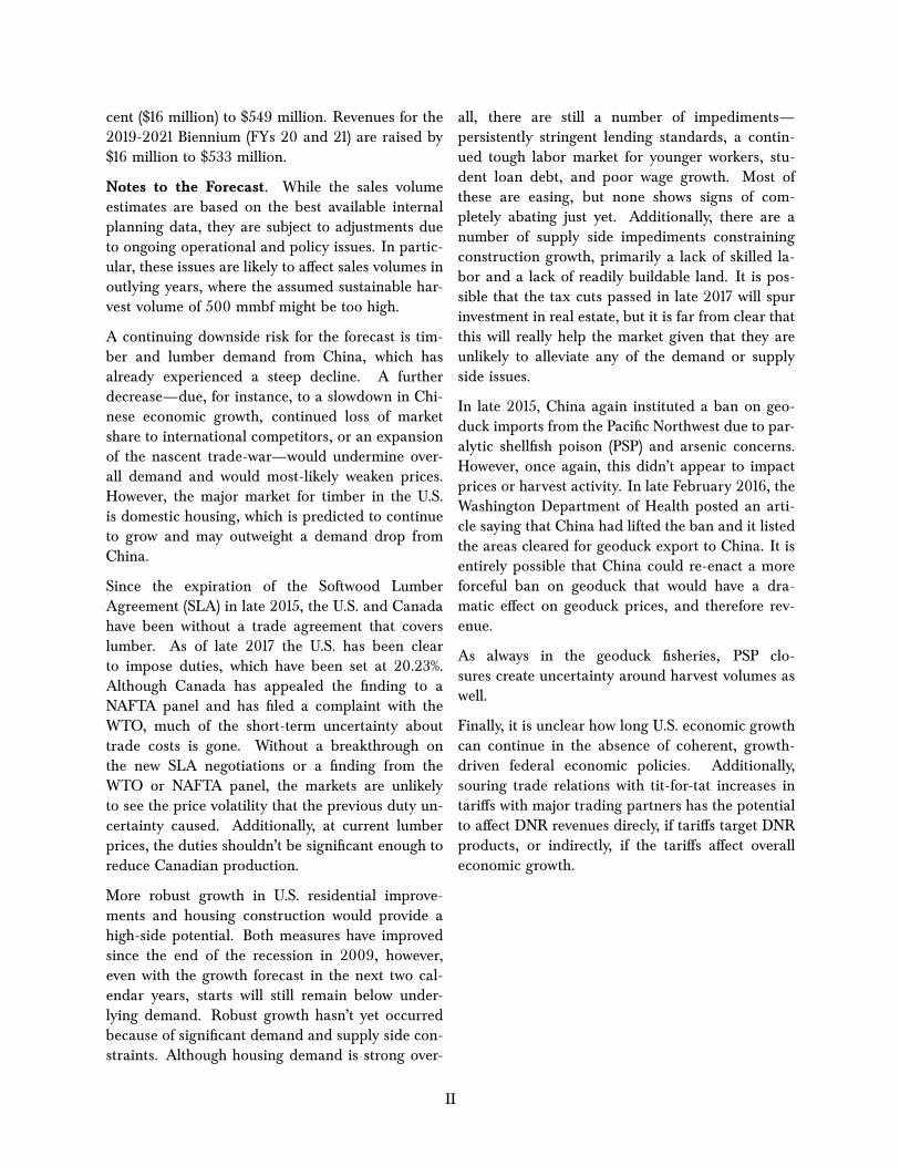
Forecast Summary

Lumber and Log Prices. Lumber prices in2017 increased through the year from $350/mbfto $490/mbf, averaging $425/mbf for the year—significantly higher than previous years and thehighest prices in real terms since the height of theprevious housing boom in 2005.Prices have con-tinued to increase in 2018, averaging $537/mbfthrough April.

Prices for the ‘typical’ DNR log were also markedlyhigher in 2017 than previous years, climbing from$578/mbf to $719/mbf to average $611/mbf for theyear. Again, prices for DNR logs have continuedto increase in 2018 and have averaged $723/mbfthrough April. Prices are expected to weaken in thefinal two quarters of 2018, though they will remainabove recent years’ averages, before climbing backto near current levels.

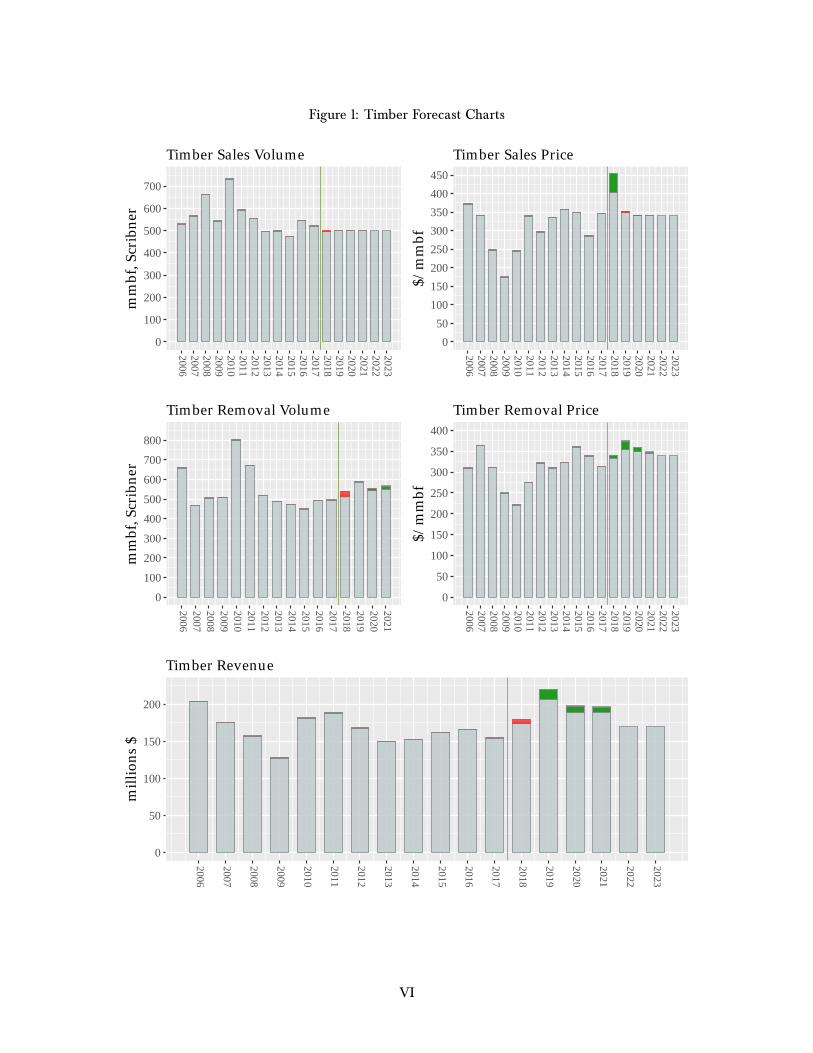
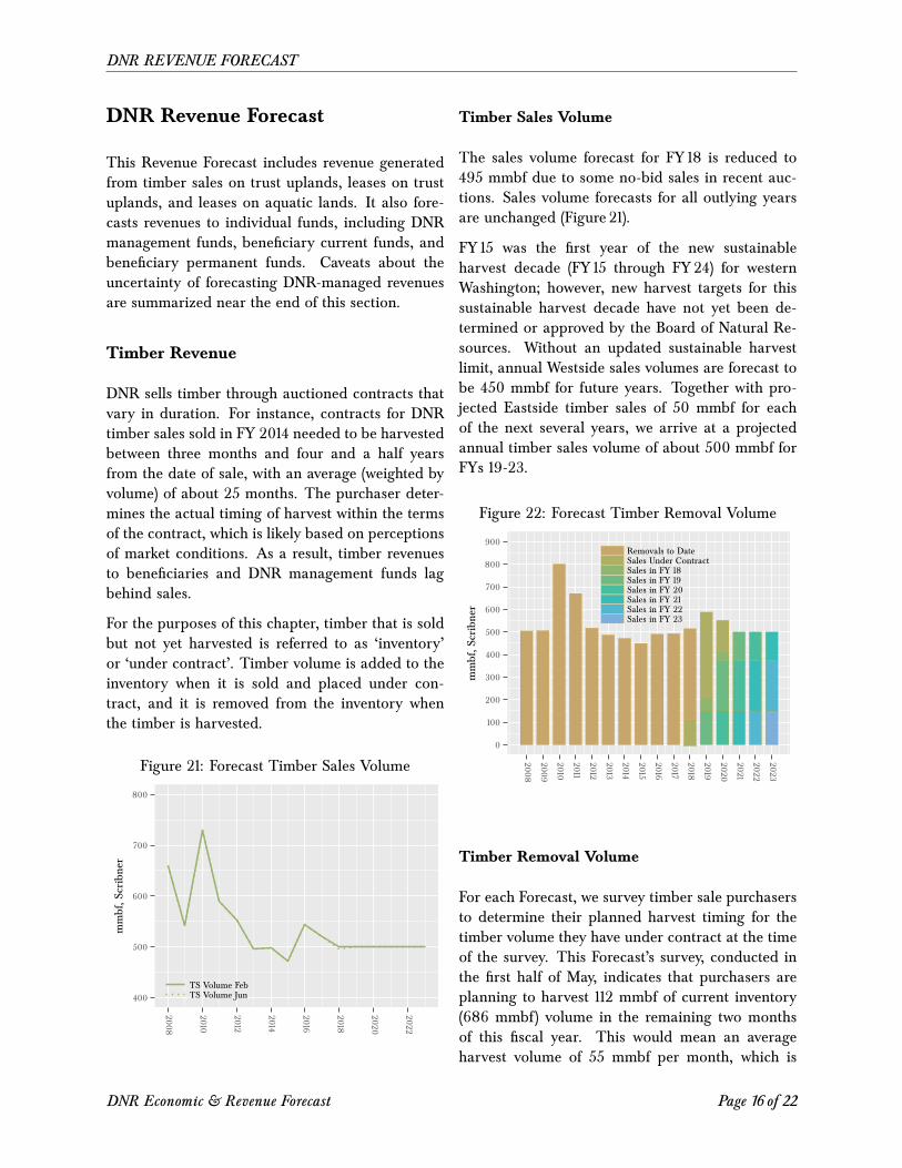
Timber Sales Volume. The sales volume forecastfor FY 18 is reduced to 495 mmbf due to some re-cent no-bid sales at auction. Sales plans in outlyingyears have not changed, so absent a new sustain-able harvest calculation, sales volume forecasts inthose years remain at 500 mmbf.

Timber Sales Prices. FY 17 auction prices aver-aged $346/mbf. To-date, auction prices for FY 18have averaged $460/mbf with over 90 percent ofthe forecast volume sold. The sales price forecastfor FY 18 is increased to $453/mbf. The sales priceforecasts for outlying years are unchanged, despiteexpectations for increases in log prices. This is be-cause there are a number of risks to house pricesand the broader economy that could adversely af-fect log and stumpage prices.

Timber Removal Volume and Prices. Account-ing for changes to purchaser plans, the timing ofcontract expirations and likely average monthlyharvests, FY 18 harvest volume expectations arelowered by 25 mmbf to 514 mmbf. Previous pur-chaser surveys indicated that timber purchasers hadmore ambitious harvest plans than eventuated. TheFY 19 harvest volume forecast is increased slightlyby 2 mmbf to 587 mmbf. Harvest volume forecastsfor FYs 20 and 21 are increased by 10 mmbf and 14

mmf, respectively.

The average timber removal price for FY 18 isincreased to $339/mbf, due to increased auctionprices and an increase in the value of remaininginventory. Timber removal prices for FYs 19-21 areprojected to be about $374 (+$21), $358 (+$10), and$347 (+$3) per mbf. These removal prices reflectchanges in both the sales prices and removal tim-ing.

Timber Revenue. The above changes to timbersales prices, sales volumes, and harvest timing haveshifted projected revenue through FY 21. Revenuesfor the 2017-2019 biennium are forecast to total$394 million, an increase of around two percent ($8million) from September’s forecast. Forecast rev-enues for the 2019-2021 biennium are increased byfour percent ($16 million) to $393 million.

Non-Timber Revenues. In addition to revenuefrom timber removals on state-managed lands,DNR also generates sizable revenues from manag-ing leases on uplands and aquatic lands.

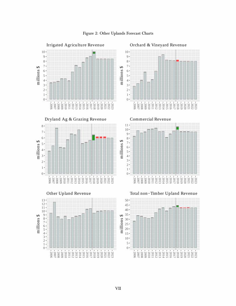
The upland lease revenue forecast for FY 18 isincreased by $2 million to $45 million due toincreases in revenue expectations for irrigatedand dryland agriculture, and commercial prop-erty outweighing decreased expectations for or-chard/vineyard agriculture. Revenue forecasts foroutlying years are decreased marginally from theprevious forecast to $42 million, due to revised ex-pectations for grazing leases.

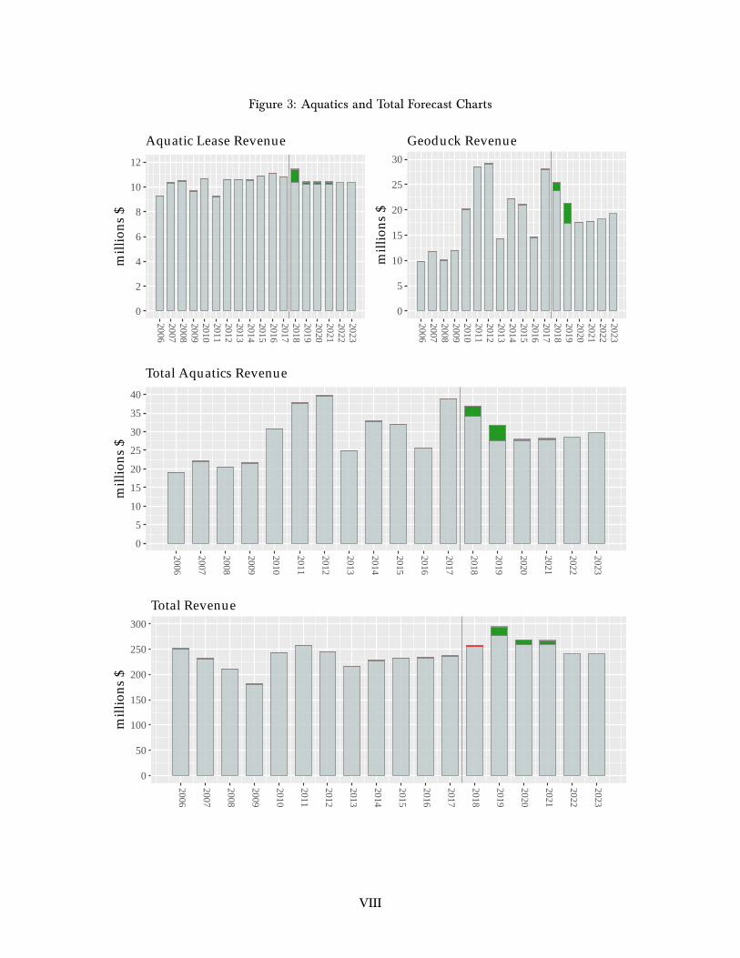
Aquatic lease revenue expectations are higher inFY 18, increased to $11 million, due to betterthan expected revenue for every type of aquaticlease. Revenues in outlying years are also in-creased slightly, to $10 million, due to a betteroutlook for both water-dependent and non-water-dependent leases.

The FY 18 geoduck revenue is increased by $2 mil-lion to $25 million and FY 19 revenue is increasedby $4 million due to higher than expected auctionprices to-date and an increase in sales volume. Theremaining outlying years are unchanged.

Total Revenues. Total revenues for the 2017-2019Biennium (FYs 18-19) are increased by three per-

I

cent ($16 million) to $549 million. Revenues for the2019-2021 Biennium (FYs 20 and 21) are raised by$16 million to $533 million.

Notes to the Forecast. While the sales volumeestimates are based on the best available internalplanning data, they are subject to adjustments dueto ongoing operational and policy issues. In partic-ular, these issues are likely to affect sales volumes inoutlying years, where the assumed sustainable har-vest volume of 500 mmbf might be too high.

A continuing downside risk for the forecast is tim-ber and lumber demand from China, which hasalready experienced a steep decline. A furtherdecrease—due, for instance, to a slowdown in Chi-nese economic growth, continued loss of marketshare to international competitors, or an expansionof the nascent trade-war—would undermine over-all demand and would most-likely weaken prices.However, the major market for timber in the U.S.is domestic housing, which is predicted to continueto grow and may outweight a demand drop fromChina.

Since the expiration of the Softwood LumberAgreement (SLA) in late 2015, the U.S. and Canadahave been without a trade agreement that coverslumber. As of late 2017 the U.S. has been clearto impose duties, which have been set at 20.23%.Although Canada has appealed the finding to aNAFTA panel and has filed a complaint with theWTO, much of the short-term uncertainty abouttrade costs is gone. Without a breakthrough onthe new SLA negotiations or a finding from theWTO or NAFTA panel, the markets are unlikelyto see the price volatility that the previous duty un-certainty caused. Additionally, at current lumberprices, the duties shouldn’t be significant enough toreduce Canadian production.

More robust growth in U.S. residential improve-ments and housing construction would provide ahigh-side potential. Both measures have improvedsince the end of the recession in 2009, however,even with the growth forecast in the next two cal-endar years, starts will still remain below under-lying demand. Robust growth hasn’t yet occurredbecause of significant demand and supply side con-straints. Although housing demand is strong over-

all, there are still a number of impediments—persistently stringent lending standards, a contin-ued tough labor market for younger workers, stu-dent loan debt, and poor wage growth. Most ofthese are easing, but none shows signs of com-pletely abating just yet. Additionally, there are anumber of supply side impediments constrainingconstruction growth, primarily a lack of skilled la-bor and a lack of readily buildable land. It is pos-sible that the tax cuts passed in late 2017 will spurinvestment in real estate, but it is far from clear thatthis will really help the market given that they areunlikely to alleviate any of the demand or supplyside issues.

In late 2015, China again instituted a ban on geo-duck imports from the Pacific Northwest due to par-alytic shellfish poison (PSP) and arsenic concerns.However, once again, this didn’t appear to impactprices or harvest activity. In late February 2016, theWashington Department of Health posted an arti-cle saying that China had lifted the ban and it listedthe areas cleared for geoduck export to China. It isentirely possible that China could re-enact a moreforceful ban on geoduck that would have a dra-matic effect on geoduck prices, and therefore rev-enue.

As always in the geoduck fisheries, PSP clo-sures create uncertainty around harvest volumes aswell.

Finally, it is unclear how long U.S. economic growthcan continue in the absence of coherent, growth-driven federal economic policies. Additionally,souring trade relations with tit-for-tat increases intariffs with major trading partners has the potentialto affect DNR revenues direcly, if tariffs target DNRproducts, or indirectly, if the tariffs affect overalleconomic growth.

II

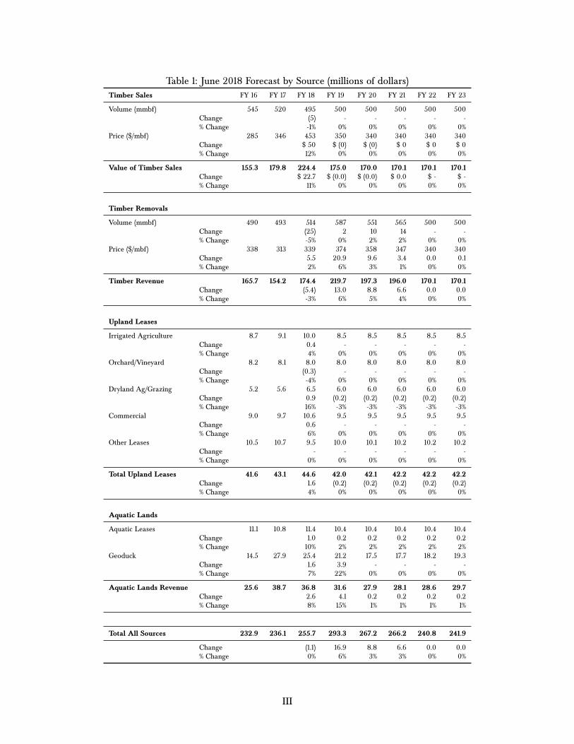
Table 1: June 2018 Forecast by Source (millions of dollars)Timber Sales FY 16 FY 17 FY 18 FY 19 FY 20 FY 21 FY 22 FY 23

Volume (mmbf) 545 520 495 500 500 500 500 500Change (5) - - - - -% Change -1% 0% 0% 0% 0% 0%

Price ($/mbf) 285 346 453 350 340 340 340 340Change $ 50 $ (0) $ (0) $ 0 $ 0 $ 0% Change 12% 0% 0% 0% 0% 0%

Value of Timber Sales 155.3 179.8 224.4 175.0 170.0 170.1 170.1 170.1Change $ 22.7 $ (0.0) $ (0.0) $ 0.0 $ - $ -% Change 11% 0% 0% 0% 0% 0%

Timber Removals

Volume (mmbf) 490 493 514 587 551 565 500 500Change (25) 2 10 14 - -% Change -5% 0% 2% 2% 0% 0%

Price ($/mbf) 338 313 339 374 358 347 340 340Change 5.5 20.9 9.6 3.4 0.0 0.1% Change 2% 6% 3% 1% 0% 0%

Timber Revenue 165.7 154.2 174.4 219.7 197.3 196.0 170.1 170.1Change (5.4) 13.0 8.8 6.6 0.0 0.0% Change -3% 6% 5% 4% 0% 0%

Upland Leases

Irrigated Agriculture 8.7 9.1 10.0 8.5 8.5 8.5 8.5 8.5Change 0.4 - - - - -% Change 4% 0% 0% 0% 0% 0%

Orchard/Vineyard 8.2 8.1 8.0 8.0 8.0 8.0 8.0 8.0Change (0.3) - - - - -% Change -4% 0% 0% 0% 0% 0%

Dryland Ag/Grazing 5.2 5.6 6.5 6.0 6.0 6.0 6.0 6.0Change 0.9 (0.2) (0.2) (0.2) (0.2) (0.2)% Change 16% -3% -3% -3% -3% -3%

Commercial 9.0 9.7 10.6 9.5 9.5 9.5 9.5 9.5Change 0.6 - - - - -% Change 6% 0% 0% 0% 0% 0%

Other Leases 10.5 10.7 9.5 10.0 10.1 10.2 10.2 10.2Change - - - - - -% Change 0% 0% 0% 0% 0% 0%

Total Upland Leases 41.6 43.1 44.6 42.0 42.1 42.2 42.2 42.2Change 1.6 (0.2) (0.2) (0.2) (0.2) (0.2)% Change 4% 0% 0% 0% 0% 0%

Aquatic Lands

Aquatic Leases 11.1 10.8 11.4 10.4 10.4 10.4 10.4 10.4Change 1.0 0.2 0.2 0.2 0.2 0.2% Change 10% 2% 2% 2% 2% 2%

Geoduck 14.5 27.9 25.4 21.2 17.5 17.7 18.2 19.3Change 1.6 3.9 - - - -% Change 7% 22% 0% 0% 0% 0%

Aquatic Lands Revenue 25.6 38.7 36.8 31.6 27.9 28.1 28.6 29.7Change 2.6 4.1 0.2 0.2 0.2 0.2% Change 8% 15% 1% 1% 1% 1%

Total All Sources 232.9 236.1 255.7 293.3 267.2 266.2 240.8 241.9

Change (1.1) 16.9 8.8 6.6 0.0 0.0% Change 0% 6% 3% 3% 0% 0%

III

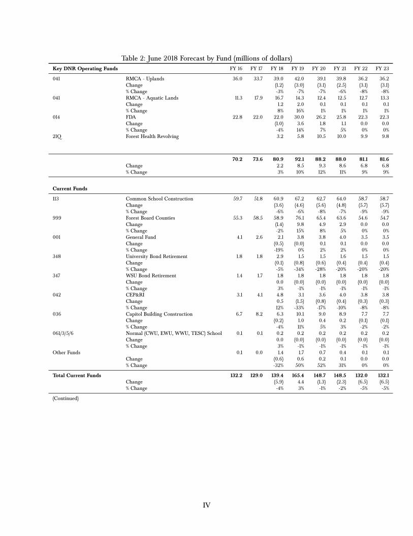
Table 2: June 2018 Forecast by Fund (millions of dollars)Key DNR Operating Funds FY 16 FY 17 FY 18 FY 19 FY 20 FY 21 FY 22 FY 23

041 RMCA - Uplands 36.0 33.7 39.0 42.0 39.1 39.8 36.2 36.2Change (1.2) (3.0) (3.1) (2.5) (3.1) (3.1)% Change -3% -7% -7% -6% -8% -8%

041 RMCA - Aquatic Lands 11.3 17.9 16.7 14.3 12.4 12.5 12.7 13.3Change 1.2 2.0 0.1 0.1 0.1 0.1% Change 8% 16% 1% 1% 1% 1%

014 FDA 22.8 22.0 22.0 30.0 26.2 25.8 22.3 22.3Change (1.0) 3.6 1.8 1.1 0.0 0.0% Change -4% 14% 7% 5% 0% 0%

21Q Forest Health Revolving 3.2 5.8 10.5 10.0 9.9 9.8

70.2 73.6 80.9 92.1 88.2 88.0 81.1 81.6Change 2.2 8.5 9.3 8.6 6.8 6.8% Change 3% 10% 12% 11% 9% 9%

Current Funds

113 Common School Construction 59.7 51.8 60.9 67.2 62.7 64.0 58.7 58.7Change (3.6) (4.6) (5.6) (4.8) (5.7) (5.7)% Change -6% -6% -8% -7% -9% -9%

999 Forest Board Counties 55.3 58.5 58.9 76.1 65.4 63.6 54.6 54.7Change (1.4) 9.8 4.9 2.9 0.0 0.0% Change -2% 15% 8% 5% 0% 0%

001 General Fund 4.1 2.6 2.1 3.8 3.8 4.0 3.5 3.5Change (0.5) (0.0) 0.1 0.1 0.0 0.0% Change -19% 0% 2% 2% 0% 0%

348 University Bond Retirement 1.8 1.8 2.9 1.5 1.5 1.6 1.5 1.5Change (0.1) (0.8) (0.6) (0.4) (0.4) (0.4)% Change -5% -34% -28% -20% -20% -20%

347 WSU Bond Retirement 1.4 1.7 1.8 1.8 1.8 1.8 1.8 1.8Change 0.0 (0.0) (0.0) (0.0) (0.0) (0.0)% Change 3% -1% -1% -1% -1% -1%

042 CEP&RI 3.1 4.1 4.8 3.1 3.6 4.0 3.8 3.8Change 0.5 (1.5) (0.8) (0.4) (0.3) (0.3)% Change 12% -33% -17% -10% -8% -8%

036 Capitol Building Construction 6.7 8.2 6.3 10.1 9.0 8.9 7.7 7.7Change (0.2) 1.0 0.4 0.2 (0.1) (0.1)% Change -4% 11% 5% 3% -2% -2%

061/3/5/6 Normal (CWU, EWU, WWU, TESC) School 0.1 0.1 0.2 0.2 0.2 0.2 0.2 0.2Change 0.0 (0.0) (0.0) (0.0) (0.0) (0.0)% Change 3% -1% -1% -1% -1% -1%

Other Funds 0.1 0.0 1.4 1.7 0.7 0.4 0.1 0.1Change (0.6) 0.6 0.2 0.1 0.0 0.0% Change -32% 50% 52% 31% 0% 0%

Total Current Funds 132.2 129.0 139.4 165.4 148.7 148.5 132.0 132.1Change (5.9) 4.4 (1.3) (2.3) (6.5) (6.5)% Change -4% 3% -1% -2% -5% -5%

(Continued)

IV

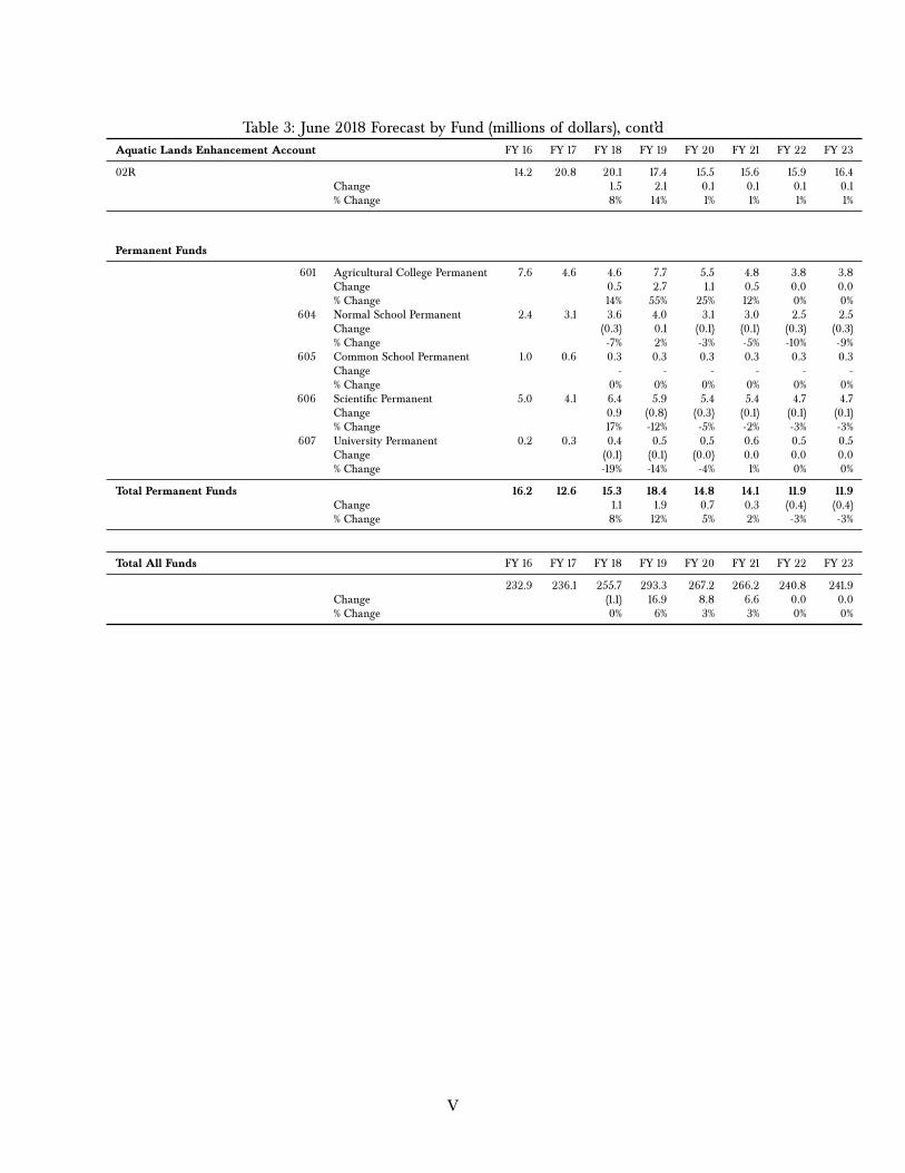
Table 3: June 2018 Forecast by Fund (millions of dollars), cont’dAquatic Lands Enhancement Account FY 16 FY 17 FY 18 FY 19 FY 20 FY 21 FY 22 FY 23

02R 14.2 20.8 20.1 17.4 15.5 15.6 15.9 16.4Change 1.5 2.1 0.1 0.1 0.1 0.1% Change 8% 14% 1% 1% 1% 1%

Permanent Funds

601 Agricultural College Permanent 7.6 4.6 4.6 7.7 5.5 4.8 3.8 3.8Change 0.5 2.7 1.1 0.5 0.0 0.0% Change 14% 55% 25% 12% 0% 0%

604 Normal School Permanent 2.4 3.1 3.6 4.0 3.1 3.0 2.5 2.5Change (0.3) 0.1 (0.1) (0.1) (0.3) (0.3)% Change -7% 2% -3% -5% -10% -9%

605 Common School Permanent 1.0 0.6 0.3 0.3 0.3 0.3 0.3 0.3Change - - - - - -% Change 0% 0% 0% 0% 0% 0%

606 Scientific Permanent 5.0 4.1 6.4 5.9 5.4 5.4 4.7 4.7Change 0.9 (0.8) (0.3) (0.1) (0.1) (0.1)% Change 17% -12% -5% -2% -3% -3%

607 University Permanent 0.2 0.3 0.4 0.5 0.5 0.6 0.5 0.5Change (0.1) (0.1) (0.0) 0.0 0.0 0.0% Change -19% -14% -4% 1% 0% 0%

Total Permanent Funds 16.2 12.6 15.3 18.4 14.8 14.1 11.9 11.9Change 1.1 1.9 0.7 0.3 (0.4) (0.4)% Change 8% 12% 5% 2% -3% -3%

Total All Funds FY 16 FY 17 FY 18 FY 19 FY 20 FY 21 FY 22 FY 23

232.9 236.1 255.7 293.3 267.2 266.2 240.8 241.9Change (1.1) 16.9 8.8 6.6 0.0 0.0% Change 0% 6% 3% 3% 0% 0%

V

0

100

200

300

400

500

600

700

200620072008200920102011201220132014201520162017201820192020202120222023

mm

bf, S

crib

ner

Timber Sales Volume

0

50

100

150

200

250

300

350

400

450

200620072008200920102011201220132014201520162017201820192020202120222023

$/m

mbf

Timber Sales Price

0

100

200

300

400

500

600

700

800

2006200720082009201020112012201320142015201620172018201920202021

mm

bf, S

crib

ner

Timber Removal Volume

0

50

100

150

200

250

300

350

400

200620072008200920102011201220132014201520162017201820192020202120222023

$/m

mbf

Timber Removal Price

0

50

100

150

200

2006

2007

2008

2009

2010

2011

2012

2013

2014

2015

2016

2017

2018

2019

2020

2021

2022

2023

mill

ions

$

Timber Revenue

0

100

200

300

400

500

600

700

200620072008200920102011201220132014201520162017201820192020202120222023

mm

bf, S

crib

ner

Timber Sales Volume

0

50

100

150

200

250

300

350

400

450

200620072008200920102011201220132014201520162017201820192020202120222023

$/m

mbf

Timber Sales Price

0

100

200

300

400

500

600

700

800

2006200720082009201020112012201320142015201620172018201920202021

mm

bf, S

crib

ner

Timber Removal Volume

0

50

100

150

200

250

300

350

400

200620072008200920102011201220132014201520162017201820192020202120222023

$/m

mbf

Timber Removal Price

0

50

100

150

200

2006

2007

2008

2009

2010

2011

2012

2013

2014

2015

2016

2017

2018

2019

2020

2021

2022

2023

mill

ions

$

Timber Revenue

Figure 1: Timber Forecast Charts

VI

0123456789

10

200620072008200920102011201220132014201520162017201820192020202120222023

mill

ions

$

Irrigated Agriculture Revenue

0123456789

10

200620072008200920102011201220132014201520162017201820192020202120222023

mill

ions

$

Orchard & Vineyard Revenue

0

1

2

3

4

5

6

7

8

200620072008200920102011201220132014201520162017201820192020202120222023

mill

ions

$

Dryland Ag & Grazing Revenue

0123456789

1011

200620072008200920102011201220132014201520162017201820192020202120222023

mill

ions

$Commercial Revenue

0123456789

10111213

200620072008200920102011201220132014201520162017201820192020202120222023

mill

ions

$

Other Upland Revenue

05

101520253035404550

200620072008200920102011201220132014201520162017201820192020202120222023

mill

ions

$

Total non−Timber Upland Revenue

0123456789

10

200620072008200920102011201220132014201520162017201820192020202120222023

mill

ions

$

Irrigated Agriculture Revenue

0123456789

10

200620072008200920102011201220132014201520162017201820192020202120222023

mill

ions

$

Orchard & Vineyard Revenue

0

1

2

3

4

5

6

7

8

200620072008200920102011201220132014201520162017201820192020202120222023

mill

ions

$

Dryland Ag & Grazing Revenue

0123456789

1011

200620072008200920102011201220132014201520162017201820192020202120222023

mill

ions

$Commercial Revenue

0123456789

10111213

200620072008200920102011201220132014201520162017201820192020202120222023

mill

ions

$

Other Upland Revenue

05

101520253035404550

200620072008200920102011201220132014201520162017201820192020202120222023

mill

ions

$

Total non−Timber Upland Revenue

Figure 2: Other Uplands Forecast Charts

VII

0

2

4

6

8

10

12

200620072008200920102011201220132014201520162017201820192020202120222023

mill

ions

$

Aquatic Lease Revenue

0

5

10

15

20

25

30

200620072008200920102011201220132014201520162017201820192020202120222023

mill

ions

$

Geoduck Revenue

0

5

10

15

20

25

30

35

40

2006

2007

2008

2009

2010

2011

2012

2013

2014

2015

2016

2017

2018

2019

2020

2021

2022

2023

mill

ions

$

Total Aquatics Revenue

0

50

100

150

200

250

300

2006

2007

2008

2009

2010

2011

2012

2013

2014

2015

2016

2017

2018

2019

2020

2021

2022

2023

mill

ions

$

Total Revenue

0

2

4

6

8

10

12

200620072008200920102011201220132014201520162017201820192020202120222023

mill

ions

$

Aquatic Lease Revenue

0

5

10

15

20

25

30

200620072008200920102011201220132014201520162017201820192020202120222023

mill

ions

$

Geoduck Revenue

0

5

10

15

20

25

30

35

40

2006

2007

2008

2009

2010

2011

2012

2013

2014

2015

2016

2017

2018

2019

2020

2021

2022

2023

mill

ions

$

Total Aquatics Revenue

0

50

100

150

200

250

300

2006

2007

2008

2009

2010

2011

2012

2013

2014

2015

2016

2017

2018

2019

2020

2021

2022

2023

mill

ions

$

Total Revenue

Figure 3: Aquatics and Total Forecast Charts

VIII

Contents

Forecast Summary I

Macroeconomic Conditions 1U.S. Economy . . . . . . . . . . . . . . . . . . . . . . . . . . . . . . . . . . . . . . . . . . . . . . . 1

Gross Domestic Product . . . . . . . . . . . . . . . . . . . . . . . . . . . . . . . . . . . . . . 1Employment and Wages . . . . . . . . . . . . . . . . . . . . . . . . . . . . . . . . . . . . . . 1Inflation . . . . . . . . . . . . . . . . . . . . . . . . . . . . . . . . . . . . . . . . . . . . . . 3Interest Rates . . . . . . . . . . . . . . . . . . . . . . . . . . . . . . . . . . . . . . . . . . . 3The U.S. Dollar and Foreign Trade . . . . . . . . . . . . . . . . . . . . . . . . . . . . . . . . 4Petroleum . . . . . . . . . . . . . . . . . . . . . . . . . . . . . . . . . . . . . . . . . . . . . . 5

World Economy . . . . . . . . . . . . . . . . . . . . . . . . . . . . . . . . . . . . . . . . . . . . . 6Europe . . . . . . . . . . . . . . . . . . . . . . . . . . . . . . . . . . . . . . . . . . . . . . . 6China . . . . . . . . . . . . . . . . . . . . . . . . . . . . . . . . . . . . . . . . . . . . . . . . 6Japan . . . . . . . . . . . . . . . . . . . . . . . . . . . . . . . . . . . . . . . . . . . . . . . . 7

Wood Markets 8U.S. Housing Market . . . . . . . . . . . . . . . . . . . . . . . . . . . . . . . . . . . . . . . . . . . 9

New Home Sales . . . . . . . . . . . . . . . . . . . . . . . . . . . . . . . . . . . . . . . . . . 9Household Formation . . . . . . . . . . . . . . . . . . . . . . . . . . . . . . . . . . . . . . . 10Housing Starts . . . . . . . . . . . . . . . . . . . . . . . . . . . . . . . . . . . . . . . . . . . 10Housing Prices . . . . . . . . . . . . . . . . . . . . . . . . . . . . . . . . . . . . . . . . . . . 11

Export Markets . . . . . . . . . . . . . . . . . . . . . . . . . . . . . . . . . . . . . . . . . . . . . . 11Timber Supply . . . . . . . . . . . . . . . . . . . . . . . . . . . . . . . . . . . . . . . . . . . . . . 12Price Outlook . . . . . . . . . . . . . . . . . . . . . . . . . . . . . . . . . . . . . . . . . . . . . . . 13

Lumber Prices . . . . . . . . . . . . . . . . . . . . . . . . . . . . . . . . . . . . . . . . . . . 13Log Prices . . . . . . . . . . . . . . . . . . . . . . . . . . . . . . . . . . . . . . . . . . . . . 13Stumpage Prices . . . . . . . . . . . . . . . . . . . . . . . . . . . . . . . . . . . . . . . . . . 14DNR Stumpage Price Outlook . . . . . . . . . . . . . . . . . . . . . . . . . . . . . . . . . . 14

DNR Revenue Forecast 16Timber Revenue . . . . . . . . . . . . . . . . . . . . . . . . . . . . . . . . . . . . . . . . . . . . . 16

Timber Sales Volume . . . . . . . . . . . . . . . . . . . . . . . . . . . . . . . . . . . . . . . 16Timber Removal Volume . . . . . . . . . . . . . . . . . . . . . . . . . . . . . . . . . . . . . 16Timber Sales Prices . . . . . . . . . . . . . . . . . . . . . . . . . . . . . . . . . . . . . . . . 17Timber Removal Prices . . . . . . . . . . . . . . . . . . . . . . . . . . . . . . . . . . . . . . 17Timber Removal Revenue . . . . . . . . . . . . . . . . . . . . . . . . . . . . . . . . . . . . 18

Upland Lease Revenues . . . . . . . . . . . . . . . . . . . . . . . . . . . . . . . . . . . . . . . . . 19Aquatic Lands Revenues . . . . . . . . . . . . . . . . . . . . . . . . . . . . . . . . . . . . . . . . 20Total Revenues from All Sources . . . . . . . . . . . . . . . . . . . . . . . . . . . . . . . . . . . . 21

Some Caveats . . . . . . . . . . . . . . . . . . . . . . . . . . . . . . . . . . . . . . . . . . . 21Distribution of Revenues . . . . . . . . . . . . . . . . . . . . . . . . . . . . . . . . . . . . . . . . 22

List of Tables

1 June 2018 Forecast by Source (millions of dollars) . . . . . . . . . . . . . . . . . . . . . . . III2 June 2018 Forecast by Fund (millions of dollars) . . . . . . . . . . . . . . . . . . . . . . . . IV3 June 2018 Forecast by Fund (millions of dollars), cont’d . . . . . . . . . . . . . . . . . . . . V

List of Figures

1 Timber Forecast Charts . . . . . . . . . . . . . . . . . . . . . . . . . . . . . . . . . . . . . . VI2 Other Uplands Forecast Charts . . . . . . . . . . . . . . . . . . . . . . . . . . . . . . . . . . VII3 Aquatics and Total Forecast Charts . . . . . . . . . . . . . . . . . . . . . . . . . . . . . . . VIII4 U.S. Gross Domestic Product . . . . . . . . . . . . . . . . . . . . . . . . . . . . . . . . . . . 15 Unemployment Rate and Monthly Change in Jobs . . . . . . . . . . . . . . . . . . . . . . . 26 Employment and Unemployment . . . . . . . . . . . . . . . . . . . . . . . . . . . . . . . . . 27 Labor Market Indicators . . . . . . . . . . . . . . . . . . . . . . . . . . . . . . . . . . . . . 38 U.S. Inflation Indices . . . . . . . . . . . . . . . . . . . . . . . . . . . . . . . . . . . . . . . 39 Trade-Weighted U.S. Dollar Index . . . . . . . . . . . . . . . . . . . . . . . . . . . . . . . . 410 Crude Oil Prices . . . . . . . . . . . . . . . . . . . . . . . . . . . . . . . . . . . . . . . . . . 611 Lumber, Log, and Stumpage Prices in Washington . . . . . . . . . . . . . . . . . . . . . . . 812 Lumber, Log, and DNR Stumpage Price Seasonality . . . . . . . . . . . . . . . . . . . . . . 813 Home Sales and Starts as a Percentage of Pre-Recession Peak . . . . . . . . . . . . . . . . 914 New Single-Family Home Sales . . . . . . . . . . . . . . . . . . . . . . . . . . . . . . . . . . 915 Housing Starts . . . . . . . . . . . . . . . . . . . . . . . . . . . . . . . . . . . . . . . . . . . 1016 Case-Shiller Existing Home Price Index . . . . . . . . . . . . . . . . . . . . . . . . . . . . . 1117 Log Export Prices . . . . . . . . . . . . . . . . . . . . . . . . . . . . . . . . . . . . . . . . . 1218 Log Export Volume . . . . . . . . . . . . . . . . . . . . . . . . . . . . . . . . . . . . . . . . 1219 DNR Composite Log Prices . . . . . . . . . . . . . . . . . . . . . . . . . . . . . . . . . . . . 1420 DNR Timber Stumpage Price . . . . . . . . . . . . . . . . . . . . . . . . . . . . . . . . . . . 1521 Forecast Timber Sales Volume . . . . . . . . . . . . . . . . . . . . . . . . . . . . . . . . . . 1622 Forecast Timber Removal Volume . . . . . . . . . . . . . . . . . . . . . . . . . . . . . . . . 1623 Forecast Timber Sales Price . . . . . . . . . . . . . . . . . . . . . . . . . . . . . . . . . . . 1724 Forecast Timber Removal Price . . . . . . . . . . . . . . . . . . . . . . . . . . . . . . . . . 1725 Forecast Timber Removal Value . . . . . . . . . . . . . . . . . . . . . . . . . . . . . . . . . 1726 Forecast Timber Removal Revenue . . . . . . . . . . . . . . . . . . . . . . . . . . . . . . . 1827 Forecast Upland Lease Revenue . . . . . . . . . . . . . . . . . . . . . . . . . . . . . . . . . 1928 Aquatic Lands Revenues . . . . . . . . . . . . . . . . . . . . . . . . . . . . . . . . . . . . . 2029 Geoduck Auction Prices . . . . . . . . . . . . . . . . . . . . . . . . . . . . . . . . . . . . . . 2030 Total Revenues . . . . . . . . . . . . . . . . . . . . . . . . . . . . . . . . . . . . . . . . . . . 21

Acronyms and Abbreviations

bbf Billion board feetBLS U.S. Bureau of Labor StatisticsCAD Canadian dollarCNY Chinese yuan (renminbi)CPI Consumer Price IndexCY Calendar Year

DNR Washington Department of Natural ResourcesECB European Central BankERFC Washington State Economic and Revenue Forecast CouncilFDA Forest Development AccountFEA Forest Economic AdvisorsFed U.S. Federal Reserve Board

FOMC Federal Open Market CommitteeFY Fiscal YearGDP Gross Domestic ProductHMI National Association of Home Builders/Wells Fargo Housing Market IndexIMF International Monetary Fund

mbf Thousand board feetmmbf Million board feetPPI Producer Price IndexQ1 First quarter of year (similarly, Q2, Q3, and Q4)QE Quantitative Easing

RCW Revised Code of WashingtonRISI Resource Information Systems, Inc.RMCA Resource Management Cost AccountSA Seasonally AdjustedSAAR Seasonally Adjusted Annual Rate

TAC Total Allowable CatchUSD U.S. DollarWDFW Washington Department of Fish and WildlifeWWPA Western Wood Products AssociationWTO World Trade Organization

Preface

This Economic and Revenue Forecast projects rev-enues from Washington state lands managed by theWashington State Department of Natural Resources(DNR). These revenues are distributed to manage-ment funds and beneficiary accounts as directed bystatute.

DNR revises its Forecast quarterly to provide up-dated information for trust beneficiaries and stateand department budgeting purposes. Each DNRForecast builds on the previous one, emphasizingongoing changes. Forecasts re-evaluate world andnational macroeconomic conditions, and the de-mand and supply for forest products and othergoods. Finally, each Forecast assesses the impactof these economic conditions on projected revenuesfrom DNR-managed lands.

DNR Forecasts provide information used in theWashington Economic and Revenue Forecast issued bythe Washington State Economic and Revenue Fore-cast Council. The release dates for DNR Forecastsare determined by the state’s forecast schedule asprescribed by RCW 82.33.020. The table below

shows the anticipated schedule for future Economicand Revenue Forecasts.

This Forecast covers fiscal years 2018 through 2023.Fiscal years for Washington State government beginJuly 1 and end June 30. For example, the currentfiscal year, Fiscal Year 2018, runs from July 1, 2017through June 30, 2018.

The baseline date (the point that designates thetransition from “actuals” to predictions) for DNRrevenues in this Forecast is April 1st, 2018. Theforecast numbers beyond that date are predictedfrom the most up-to-date DNR sales and revenuedata available, including DNR’s timber sales resultsthrough April 2018. Macroeconomic and marketoutlook data and trends are the most up-to-dateavailable as the Forecast document is being writ-ten.

Unless otherwise indicated, values are expressedin nominal terms without adjustment for infla-tion or seasonality. Therefore, interpreting trendsin the Forecast requires attention to inflationarychanges in the value of money over time, separatefrom changes attributable to other economic influ-ences.

Economic Forecast Calendar

Forecast Baseline Date Final Data and Publication Date (approximate)

September 2018 August 1, 2018 September 15, 2018November 2018 October 1, 2018 November 15, 2018February 2019 January 1, 2019 February 15, 2019June 2019 May 1, 2019 June 15, 2019

Acknowledgements

The Washington Department of Natural Resources’(DNR) Economic and Revenue Forecast is a collabora-tive effort. It is the product of information providedby private individuals and organizations, as well asDNR staff. Their contributions greatly enhance thequality of the Forecast.

Special thanks are due to those in the wood prod-ucts industry who provided information for DNR’ssurvey of timber purchasers. These busy individu-als and companies volunteered information essen-tial to forecasting the timing of timber removal vol-umes, a critical component of projecting DNR’s rev-enues on behalf of beneficiaries.

Thanks also go to DNR staff who contributed to theForecast: Koshare Eagle, Katy Mink, Tom Heller,Keith Jones, Janet Ballew, Blain Reeves, Linda Farr,Michal Rechner, and Michelle McLain. They pro-vided data and counsel, including information onmarkets and revenue flows in their areas of respon-sibility.

In the final analysis, the views expressed are ourown and may not necessarily represent the views ofthe contributors, reviewers, or DNR.

Office of Finance, Budget, and Economics

Kristoffer Larson, EconomistDavid Chertudi, Lead Economist

MACROECONOMIC CONDITIONS

Macroeconomic Conditions

This section briefly reviews macroeconomic condi-tions in the United States and world economies be-cause they influence DNR revenue—most notablythrough the bid prices for DNR timber and geo-duck auctions and lease revenues from managedlands.

U.S. Economy

Gross Domestic Product

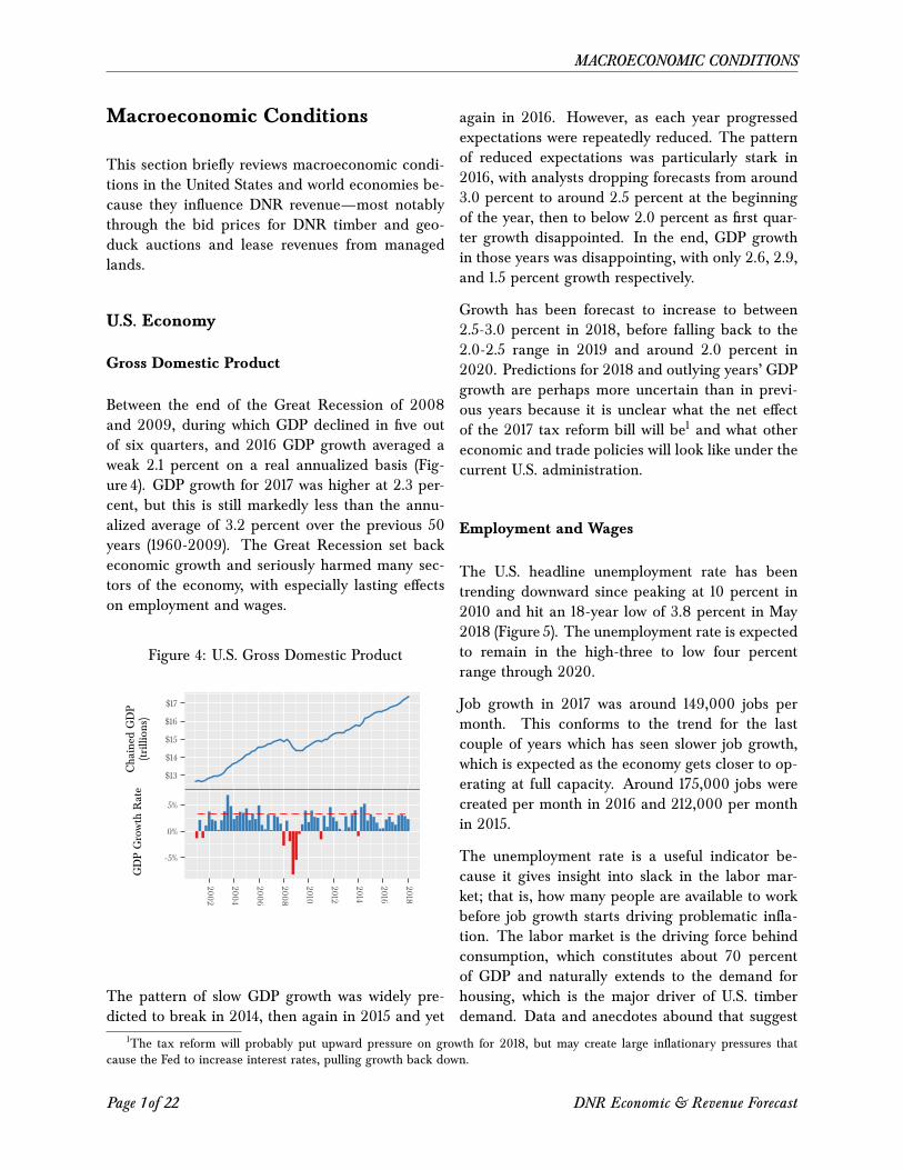
Between the end of the Great Recession of 2008and 2009, during which GDP declined in five outof six quarters, and 2016 GDP growth averaged aweak 2.1 percent on a real annualized basis (Fig-ure 4). GDP growth for 2017 was higher at 2.3 per-cent, but this is still markedly less than the annu-alized average of 3.2 percent over the previous 50years (1960-2009). The Great Recession set backeconomic growth and seriously harmed many sec-tors of the economy, with especially lasting effectson employment and wages.

Figure 4: U.S. Gross Domestic Product

$13

$14

$15

$16

$17

-5%

0%

5%

2002

2004

2006

2008

2010

2012

2014

2016

2018

Chained

GDP

(trillions)

GDPGrowth

Rate

The pattern of slow GDP growth was widely pre-dicted to break in 2014, then again in 2015 and yet

again in 2016. However, as each year progressedexpectations were repeatedly reduced. The patternof reduced expectations was particularly stark in2016, with analysts dropping forecasts from around3.0 percent to around 2.5 percent at the beginningof the year, then to below 2.0 percent as first quar-ter growth disappointed. In the end, GDP growthin those years was disappointing, with only 2.6, 2.9,and 1.5 percent growth respectively.

Growth has been forecast to increase to between2.5-3.0 percent in 2018, before falling back to the2.0-2.5 range in 2019 and around 2.0 percent in2020. Predictions for 2018 and outlying years’ GDPgrowth are perhaps more uncertain than in previ-ous years because it is unclear what the net effectof the 2017 tax reform bill will be1 and what othereconomic and trade policies will look like under thecurrent U.S. administration.

Employment and Wages

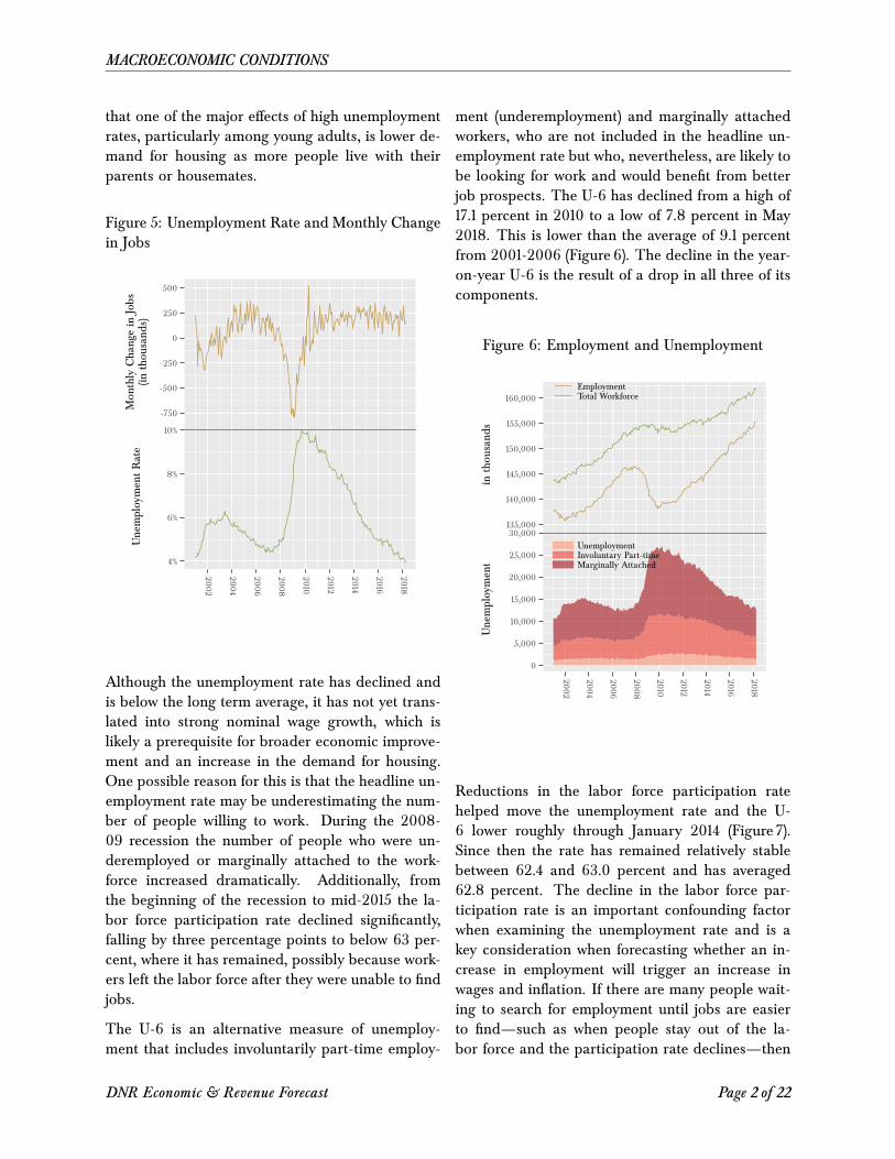
The U.S. headline unemployment rate has beentrending downward since peaking at 10 percent in2010 and hit an 18-year low of 3.8 percent in May2018 (Figure 5). The unemployment rate is expectedto remain in the high-three to low four percentrange through 2020.

Job growth in 2017 was around 149,000 jobs permonth. This conforms to the trend for the lastcouple of years which has seen slower job growth,which is expected as the economy gets closer to op-erating at full capacity. Around 175,000 jobs werecreated per month in 2016 and 212,000 per monthin 2015.

The unemployment rate is a useful indicator be-cause it gives insight into slack in the labor mar-ket; that is, how many people are available to workbefore job growth starts driving problematic infla-tion. The labor market is the driving force behindconsumption, which constitutes about 70 percentof GDP and naturally extends to the demand forhousing, which is the major driver of U.S. timberdemand. Data and anecdotes abound that suggest

1The tax reform will probably put upward pressure on growth for 2018, but may create large inflationary pressures thatcause the Fed to increase interest rates, pulling growth back down.

Page 1 of 22 DNR Economic & Revenue Forecast

MACROECONOMIC CONDITIONS

that one of the major effects of high unemploymentrates, particularly among young adults, is lower de-mand for housing as more people live with theirparents or housemates.

Figure 5: Unemployment Rate and Monthly Changein Jobs

-750

-500

-250

0

250

500

4%

6%

8%

10%

2002

2004

2006

2008

2010

2012

2014

2016

2018

Mon

thly

Changein

Jobs

(inthou

sand

s)UnemploymentRate

Although the unemployment rate has declined andis below the long term average, it has not yet trans-lated into strong nominal wage growth, which islikely a prerequisite for broader economic improve-ment and an increase in the demand for housing.One possible reason for this is that the headline un-employment rate may be underestimating the num-ber of people willing to work. During the 2008-09 recession the number of people who were un-deremployed or marginally attached to the work-force increased dramatically. Additionally, fromthe beginning of the recession to mid-2015 the la-bor force participation rate declined significantly,falling by three percentage points to below 63 per-cent, where it has remained, possibly because work-ers left the labor force after they were unable to findjobs.

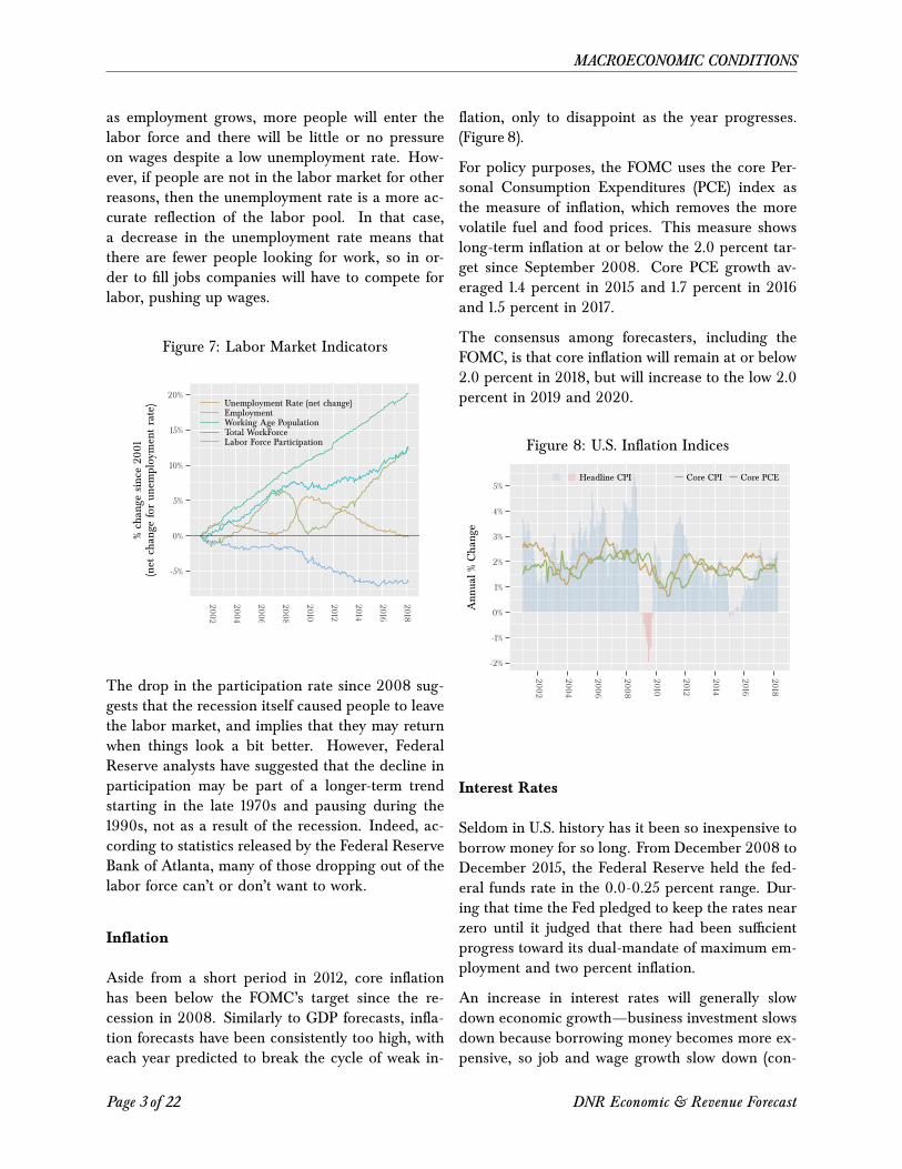
The U-6 is an alternative measure of unemploy-ment that includes involuntarily part-time employ-

ment (underemployment) and marginally attachedworkers, who are not included in the headline un-employment rate but who, nevertheless, are likely tobe looking for work and would benefit from betterjob prospects. The U-6 has declined from a high of17.1 percent in 2010 to a low of 7.8 percent in May2018. This is lower than the average of 9.1 percentfrom 2001-2006 (Figure 6). The decline in the year-on-year U-6 is the result of a drop in all three of itscomponents.

Figure 6: Employment and Unemployment

135,000

140,000

145,000

150,000

155,000

160,000

0

5,000

10,000

15,000

20,000

25,000

30,000

2002

2004

2006

2008

2010

2012

2014

2016

2018

inthou

sand

sUnemployment

EmploymentTotal Workforce

UnemploymentInvoluntary Part-timeMarginally Attached

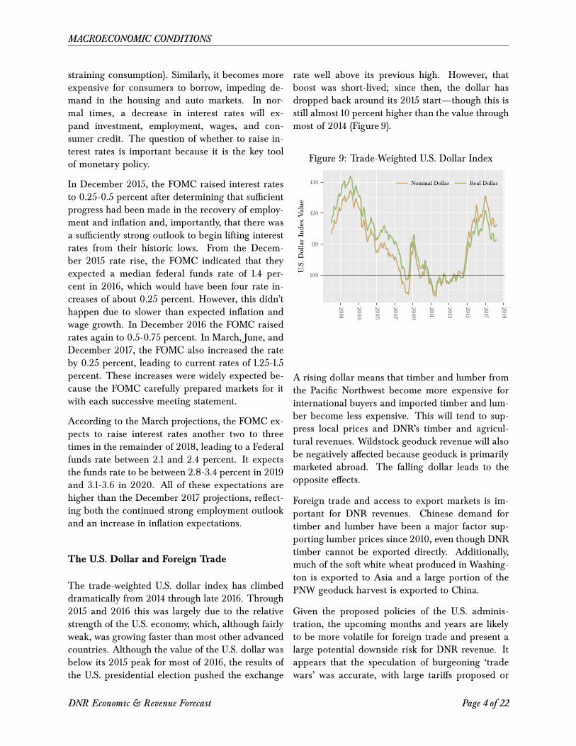
Reductions in the labor force participation ratehelped move the unemployment rate and the U-6 lower roughly through January 2014 (Figure 7).Since then the rate has remained relatively stablebetween 62.4 and 63.0 percent and has averaged62.8 percent. The decline in the labor force par-ticipation rate is an important confounding factorwhen examining the unemployment rate and is akey consideration when forecasting whether an in-crease in employment will trigger an increase inwages and inflation. If there are many people wait-ing to search for employment until jobs are easierto find—such as when people stay out of the la-bor force and the participation rate declines—then

DNR Economic & Revenue Forecast Page 2 of 22

MACROECONOMIC CONDITIONS

as employment grows, more people will enter thelabor force and there will be little or no pressureon wages despite a low unemployment rate. How-ever, if people are not in the labor market for otherreasons, then the unemployment rate is a more ac-curate reflection of the labor pool. In that case,a decrease in the unemployment rate means thatthere are fewer people looking for work, so in or-der to fill jobs companies will have to compete forlabor, pushing up wages.

Figure 7: Labor Market Indicators

-5%

0%

5%

10%

15%

20%

2002

2004

2006

2008

2010

2012

2014

2016

2018

%chan

gesince20

01(net

chan

geforun

employmentrate) Unemployment Rate (net change)

EmploymentWorking Age PopulationTotal WorkForceLabor Force Participation

The drop in the participation rate since 2008 sug-gests that the recession itself caused people to leavethe labor market, and implies that they may returnwhen things look a bit better. However, FederalReserve analysts have suggested that the decline inparticipation may be part of a longer-term trendstarting in the late 1970s and pausing during the1990s, not as a result of the recession. Indeed, ac-cording to statistics released by the Federal ReserveBank of Atlanta, many of those dropping out of thelabor force can’t or don’t want to work.

Inflation

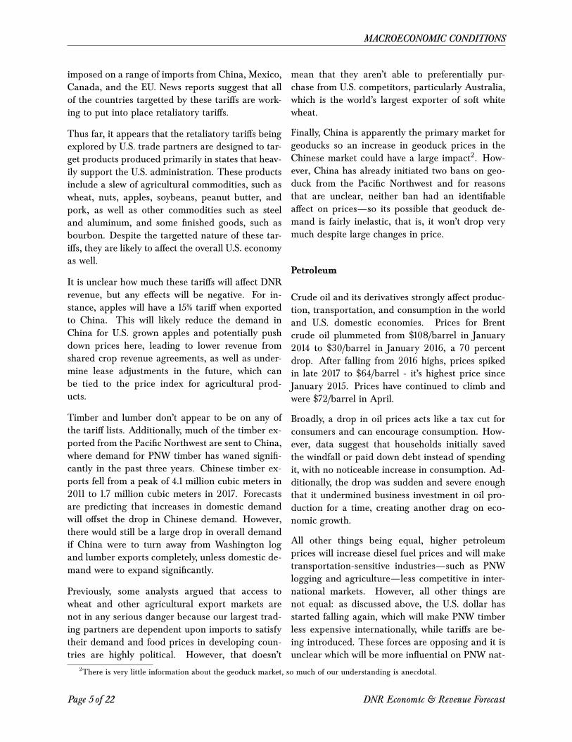
Aside from a short period in 2012, core inflationhas been below the FOMC’s target since the re-cession in 2008. Similarly to GDP forecasts, infla-tion forecasts have been consistently too high, witheach year predicted to break the cycle of weak in-

flation, only to disappoint as the year progresses.(Figure 8).

For policy purposes, the FOMC uses the core Per-sonal Consumption Expenditures (PCE) index asthe measure of inflation, which removes the morevolatile fuel and food prices. This measure showslong-term inflation at or below the 2.0 percent tar-get since September 2008. Core PCE growth av-eraged 1.4 percent in 2015 and 1.7 percent in 2016and 1.5 percent in 2017.

The consensus among forecasters, including theFOMC, is that core inflation will remain at or below2.0 percent in 2018, but will increase to the low 2.0percent in 2019 and 2020.

Figure 8: U.S. Inflation Indices

-2%

-1%

0%

1%

2%

3%

4%

5%

2002

2004

2006

2008

2010

2012

2014

2016

2018

Ann

ual%

Change

Headline CPI Core CPI Core PCE

Interest Rates

Seldom in U.S. history has it been so inexpensive toborrow money for so long. From December 2008 toDecember 2015, the Federal Reserve held the fed-eral funds rate in the 0.0-0.25 percent range. Dur-ing that time the Fed pledged to keep the rates nearzero until it judged that there had been sufficientprogress toward its dual-mandate of maximum em-ployment and two percent inflation.

An increase in interest rates will generally slowdown economic growth—business investment slowsdown because borrowing money becomes more ex-pensive, so job and wage growth slow down (con-

Page 3 of 22 DNR Economic & Revenue Forecast

MACROECONOMIC CONDITIONS

straining consumption). Similarly, it becomes moreexpensive for consumers to borrow, impeding de-mand in the housing and auto markets. In nor-mal times, a decrease in interest rates will ex-pand investment, employment, wages, and con-sumer credit. The question of whether to raise in-terest rates is important because it is the key toolof monetary policy.

In December 2015, the FOMC raised interest ratesto 0.25-0.5 percent after determining that sufficientprogress had been made in the recovery of employ-ment and inflation and, importantly, that there wasa sufficiently strong outlook to begin lifting interestrates from their historic lows. From the Decem-ber 2015 rate rise, the FOMC indicated that theyexpected a median federal funds rate of 1.4 per-cent in 2016, which would have been four rate in-creases of about 0.25 percent. However, this didn’thappen due to slower than expected inflation andwage growth. In December 2016 the FOMC raisedrates again to 0.5-0.75 percent. In March, June, andDecember 2017, the FOMC also increased the rateby 0.25 percent, leading to current rates of 1.25-1.5percent. These increases were widely expected be-cause the FOMC carefully prepared markets for itwith each successive meeting statement.

According to the March projections, the FOMC ex-pects to raise interest rates another two to threetimes in the remainder of 2018, leading to a Federalfunds rate between 2.1 and 2.4 percent. It expectsthe funds rate to be between 2.8-3.4 percent in 2019and 3.1-3.6 in 2020. All of these expectations arehigher than the December 2017 projections, reflect-ing both the continued strong employment outlookand an increase in inflation expectations.

The U.S. Dollar and Foreign Trade

The trade-weighted U.S. dollar index has climbeddramatically from 2014 through late 2016. Through2015 and 2016 this was largely due to the relativestrength of the U.S. economy, which, although fairlyweak, was growing faster than most other advancedcountries. Although the value of the U.S. dollar wasbelow its 2015 peak for most of 2016, the results ofthe U.S. presidential election pushed the exchange

rate well above its previous high. However, thatboost was short-lived; since then, the dollar hasdropped back around its 2015 start—though this isstill almost 10 percent higher than the value throughmost of 2014 (Figure 9).

Figure 9: Trade-Weighted U.S. Dollar Index

100

110

120

130

2001

2003

2005

2007

2009

2011

2013

2015

2017

2019

U.S.D

ollarIndexValue

Nominal Dollar Real Dollar

A rising dollar means that timber and lumber fromthe Pacific Northwest become more expensive forinternational buyers and imported timber and lum-ber become less expensive. This will tend to sup-press local prices and DNR’s timber and agricul-tural revenues. Wildstock geoduck revenue will alsobe negatively affected because geoduck is primarilymarketed abroad. The falling dollar leads to theopposite effects.

Foreign trade and access to export markets is im-portant for DNR revenues. Chinese demand fortimber and lumber have been a major factor sup-porting lumber prices since 2010, even though DNRtimber cannot be exported directly. Additionally,much of the soft white wheat produced in Washing-ton is exported to Asia and a large portion of thePNW geoduck harvest is exported to China.

Given the proposed policies of the U.S. adminis-tration, the upcoming months and years are likelyto be more volatile for foreign trade and present alarge potential downside risk for DNR revenue. Itappears that the speculation of burgeoning ‘tradewars’ was accurate, with large tariffs proposed or

DNR Economic & Revenue Forecast Page 4 of 22

MACROECONOMIC CONDITIONS

imposed on a range of imports from China, Mexico,Canada, and the EU. News reports suggest that allof the countries targetted by these tariffs are work-ing to put into place retaliatory tariffs.

Thus far, it appears that the retaliatory tariffs beingexplored by U.S. trade partners are designed to tar-get products produced primarily in states that heav-ily support the U.S. administration. These productsinclude a slew of agricultural commodities, such aswheat, nuts, apples, soybeans, peanut butter, andpork, as well as other commodities such as steeland aluminum, and some finished goods, such asbourbon. Despite the targetted nature of these tar-iffs, they are likely to affect the overall U.S. economyas well.

It is unclear how much these tariffs will affect DNRrevenue, but any effects will be negative. For in-stance, apples will have a 15% tariff when exportedto China. This will likely reduce the demand inChina for U.S. grown apples and potentially pushdown prices here, leading to lower revenue fromshared crop revenue agreements, as well as under-mine lease adjustments in the future, which canbe tied to the price index for agricultural prod-ucts.

Timber and lumber don’t appear to be on any ofthe tariff lists. Additionally, much of the timber ex-ported from the Pacific Northwest are sent to China,where demand for PNW timber has waned signifi-cantly in the past three years. Chinese timber ex-ports fell from a peak of 4.1 million cubic meters in2011 to 1.7 million cubic meters in 2017. Forecastsare predicting that increases in domestic demandwill offset the drop in Chinese demand. However,there would still be a large drop in overall demandif China were to turn away from Washington logand lumber exports completely, unless domestic de-mand were to expand significantly.

Previously, some analysts argued that access towheat and other agricultural export markets arenot in any serious danger because our largest trad-ing partners are dependent upon imports to satisfytheir demand and food prices in developing coun-tries are highly political. However, that doesn’t

mean that they aren’t able to preferentially pur-chase from U.S. competitors, particularly Australia,which is the world’s largest exporter of soft whitewheat.

Finally, China is apparently the primary market forgeoducks so an increase in geoduck prices in theChinese market could have a large impact2. How-ever, China has already initiated two bans on geo-duck from the Pacific Northwest and for reasonsthat are unclear, neither ban had an identifiableaffect on prices—so its possible that geoduck de-mand is fairly inelastic, that is, it won’t drop verymuch despite large changes in price.

Petroleum

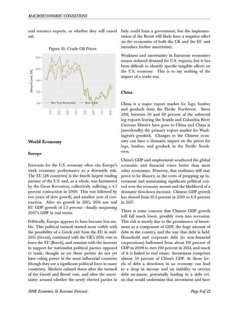
Crude oil and its derivatives strongly affect produc-tion, transportation, and consumption in the worldand U.S. domestic economies. Prices for Brentcrude oil plummeted from $108/barrel in January2014 to $30/barrel in January 2016, a 70 percentdrop. After falling from 2016 highs, prices spikedin late 2017 to $64/barrel - it’s highest price sinceJanuary 2015. Prices have continued to climb andwere $72/barrel in April.

Broadly, a drop in oil prices acts like a tax cut forconsumers and can encourage consumption. How-ever, data suggest that households initially savedthe windfall or paid down debt instead of spendingit, with no noticeable increase in consumption. Ad-ditionally, the drop was sudden and severe enoughthat it undermined business investment in oil pro-duction for a time, creating another drag on eco-nomic growth.

All other things being equal, higher petroleumprices will increase diesel fuel prices and will maketransportation-sensitive industries—such as PNWlogging and agriculture—less competitive in inter-national markets. However, all other things arenot equal: as discussed above, the U.S. dollar hasstarted falling again, which will make PNW timberless expensive internationally, while tariffs are be-ing introduced. These forces are opposing and it isunclear which will be more influential on PNW nat-

2There is very little information about the geoduck market, so much of our understanding is anecdotal.

Page 5 of 22 DNR Economic & Revenue Forecast

MACROECONOMIC CONDITIONS

ural resource exports, or whether they will cancelout.

Figure 10: Crude Oil Prices

$40

$60

$80

$100

$120

2011

2012

2013

2014

2015

2016

2017

2018

$/barrel

(real,SA

)

West Texas Intermediate Brent Crude

World Economy

Europe

Forecasts for the U.S. economy often cite Europe’sweak economic performance as a downside risk.The EU (28 countries) is the fourth largest tradingpartner of the U.S. and, as a whole, was hammeredby the Great Recession, collectively suffering a 4.5percent contraction in 2009. This was followed bytwo years of slow growth, and another year of con-traction. After no growth in 2013, 2014 saw realEU GDP growth of 1.3 percent—finally surpassing2007’s GDP in real terms.

Politically, Europe appears to have become less sta-ble. This political turmoil started most visibly withthe possibility of a Greek exit from the EU in mid-2015 (Grexit), continued with the UK’s 2016 vote toleave the EU (Brexit), and remains with the increasein support for nationalist political parties opposedto trade, thought as yet these parties do not yethave ruling power in the most influential countries(though they are a significant political force in manycountries). Markets calmed down after the turmoilof the Grexit and Brexit vote, and after the uncer-tainty around whether the newly elected parties in

Italy could form a government, but the implemen-tation of the Brexit will likely have a negative effecton the economies of both the UK and the EU andintroduce further uncertainty.

Weakness and uncertainty in Eurozone economiesmeans reduced demand for U.S. exports, but it hasbeen difficult to identify specific tangible effects onthe U.S. economy. This is to say nothing of theimpact of a trade-war.

China

China is a major export market for logs, lumberand geoduck from the Pacific Northwest. Since2011, between 50 and 60 percent of the softwoodlog exports leaving the Seattle and Columbia RiverCustoms District have gone to China and China is(anecdotally) the primary export market for Wash-ington’s geoduck. Changes to the Chinese econ-omy can have a dramatic impact on the prices forlogs, lumber, and geoduck in the Pacific North-west.

China’s GDP and employment weathered the globaleconomic and financial crises better than mostother economies. However, that resilience still mayprove to be illusory, as the costs of propping up in-vestment and maintaining significant political con-trol over the economy mount and the likelihood of adramatic slowdown increase. Chinese GDP growthhas slowed from 10.4 percent in 2010 to 6.9 percentin 2017.

There is some concern that Chinese GDP growthwill fall much lower, possibly even into recession.This risk is mostly due to the prominence of invest-ment as a component of GDP, the huge amount ofdebt in the country, and the way that debt is held.Household and corporate debt (to non-financialcorporations) ballooned from about 110 percent ofGDP in 2008 to over 190 percent in 2014, and muchof it is linked to real estate. Investment comprisesalmost 50 percent of China’s GDP. At those lev-els of debt a slowdown in an economy can leadto a drop in income and an inability to servicedebt en-masse, potentially leading to a debt cri-sis that would undermine that investment and have

DNR Economic & Revenue Forecast Page 6 of 22

MACROECONOMIC CONDITIONS

a tremendous impact on China’s GDP.

Another source of uncertainty is the current U.S.administration, which has been critical of tradewith China. China is particularly vulnerable tochanges in access to international markets, partic-ularly the U.S., with exports making up 25 per-cent of its GDP and a large proportion of employ-ment dependent upon labor-intensive export indus-tries.

Japan

Japan is another major export market for the Pa-cific Northwest—importing around 35 percent ofthe softwood logs exported from the Seattle andColumbia River customs districts since 2012. Un-fortunately, Japan’s growth has stagnated since theearly 1990s after a stock market and property bub-ble bust trapped the economy into a deflationaryspiral. After his election in late 2012, JapanesePrime Minister Shinzo Abe began a fairly boldcombination of economic policy moves, dubbed‘Abenomics’, in an attempt to revitalize Japan’seconomy. However, this effort has yet to be effec-tive.

While the Japanese economy hasn’t pulled out ofslow growth, it does not appear to be in any dangerof a recession, so it is unlikely to be a source of riskfor timber prices.

Page 7 of 22 DNR Economic & Revenue Forecast

WOOD MARKETS

Wood Markets

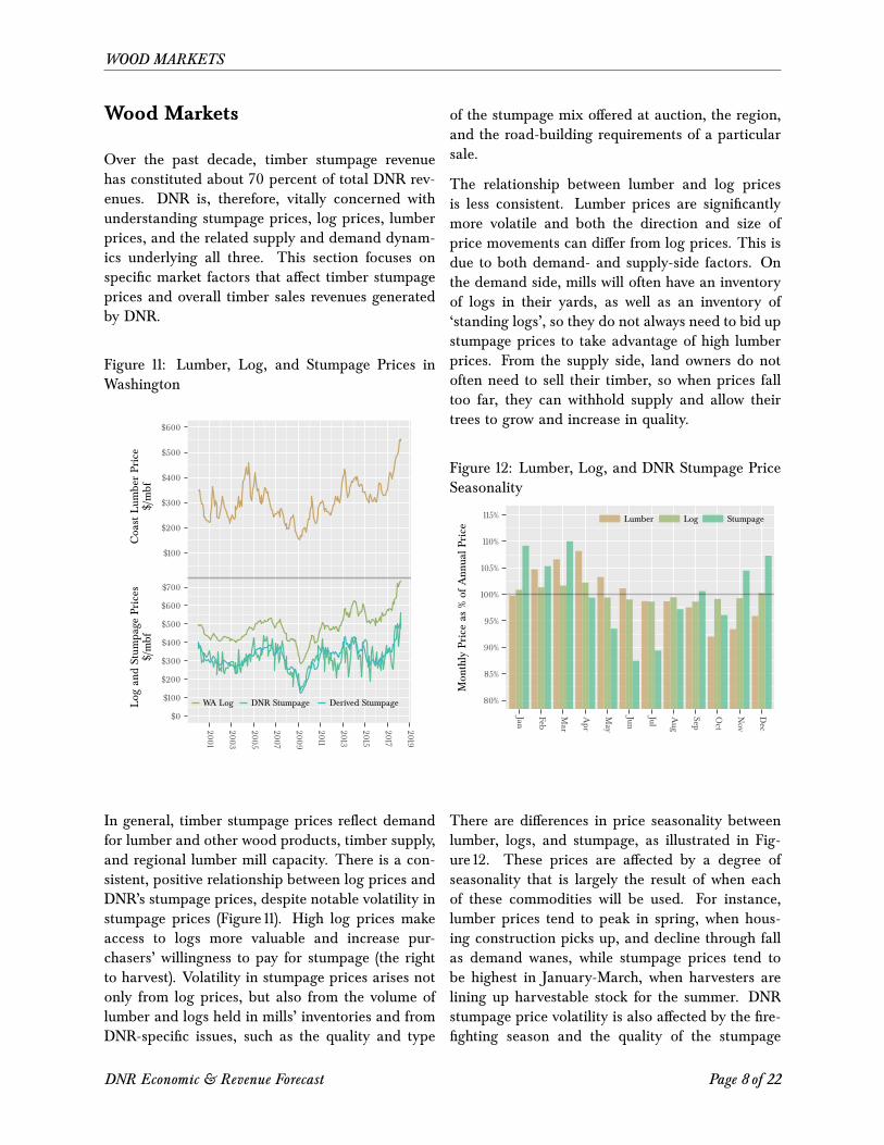
Over the past decade, timber stumpage revenuehas constituted about 70 percent of total DNR rev-enues. DNR is, therefore, vitally concerned withunderstanding stumpage prices, log prices, lumberprices, and the related supply and demand dynam-ics underlying all three. This section focuses onspecific market factors that affect timber stumpageprices and overall timber sales revenues generatedby DNR.

Figure 11: Lumber, Log, and Stumpage Prices inWashington

$100

$200

$300

$400

$500

$600

$0

$100

$200

$300

$400

$500

$600

$700

2001

2003

2005

2007

2009

2011

2013

2015

2017

2019

CoastLum

berPrice

$/mbf

Log

andStum

page

Prices

$/mbf

WA Log DNR Stumpage Derived Stumpage

In general, timber stumpage prices reflect demandfor lumber and other wood products, timber supply,and regional lumber mill capacity. There is a con-sistent, positive relationship between log prices andDNR’s stumpage prices, despite notable volatility instumpage prices (Figure 11). High log prices makeaccess to logs more valuable and increase pur-chasers’ willingness to pay for stumpage (the rightto harvest). Volatility in stumpage prices arises notonly from log prices, but also from the volume oflumber and logs held in mills’ inventories and fromDNR-specific issues, such as the quality and type

of the stumpage mix offered at auction, the region,and the road-building requirements of a particularsale.

The relationship between lumber and log pricesis less consistent. Lumber prices are significantlymore volatile and both the direction and size ofprice movements can differ from log prices. This isdue to both demand- and supply-side factors. Onthe demand side, mills will often have an inventoryof logs in their yards, as well as an inventory of‘standing logs’, so they do not always need to bid upstumpage prices to take advantage of high lumberprices. From the supply side, land owners do notoften need to sell their timber, so when prices falltoo far, they can withhold supply and allow theirtrees to grow and increase in quality.

Figure 12: Lumber, Log, and DNR Stumpage PriceSeasonality

80%

85%

90%

95%

100%

105%

110%

115%

Jan

Feb

Mar

Apr

May

Jun

Jul

Aug

Sep

Oct

Nov

Dec

Mon

thly

Priceas

%of

Ann

ualP

rice

Lumber Log Stumpage

There are differences in price seasonality betweenlumber, logs, and stumpage, as illustrated in Fig-ure 12. These prices are affected by a degree ofseasonality that is largely the result of when eachof these commodities will be used. For instance,lumber prices tend to peak in spring, when hous-ing construction picks up, and decline through fallas demand wanes, while stumpage prices tend tobe highest in January-March, when harvesters arelining up harvestable stock for the summer. DNRstumpage price volatility is also affected by the fire-fighting season and the quality of the stumpage

DNR Economic & Revenue Forecast Page 8 of 22

WOOD MARKETS

mix, which varies throughout the year but tendsto be worse from July through September.

U.S. Housing Market

This section continues with a discussion of the U.S.housing market because it is particularly importantto overall timber demand in the U.S.

New residential construction (housing starts) andresidential improvements are major components ofthe total demand for timber in the U.S. Historically,these sectors have constituted over 70 percent ofsoftwood consumption—45 percent going to hous-ing starts and 25 percent to improvements—withthe remainder going to industrial production andother applications.

Figure 13: Home Sales and Starts as a Percentageof Pre-Recession Peak

0%

10%

20%

30%

40%

50%

60%

70%

80%

90%

100%

2002

2004

2006

2008

2010

2012

2014

2016

2018

%chan

gesincemarketpeak

Existing Home SalesNew Home SalesSingle-Family Starts

The crash in the housing market and the follow-ing recession drastically reduced demand for newhousing, which undermined the total demand forlumber (Figure 13). Since the 2009-11 trough, theincrease in housing starts has driven an increase inlumber demand, though not to nearly the extent ofthe peak. Prolonged growth in starts is essentialfor a meaningful increase in the demand for lum-ber.

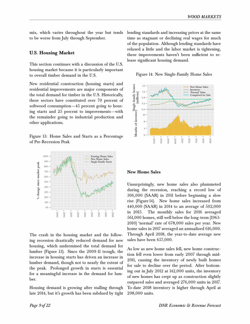
Housing demand is growing after stalling throughlate 2014, but it’s growth has been subdued by tight

lending standards and increasing prices at the sametime as stagnant or declining real wages for muchof the population. Although lending standards haverelaxed a little and the labor market is tightening,these improvements haven’t been sufficient to re-lease significant housing demand.

Figure 14: New Single-Family Home Sales

0.0

0.4

0.8

1.2

1.6

0

4

8

12

2002

2004

2006

2008

2010

2012

2014

2016

2018

Sing

le-fam

ilyho

mes

(millions)

Mon

thsof

inventory

New Home SalesInventory‘Normal’ SalesCompleted for Sale

New Home Sales

Unsurprisingly, new home sales also plummetedduring the recession, reaching a record low of306,000 (SAAR) in 2011 before beginning a slowrise (Figure 14). New home sales increased from440,000 (SAAR) in 2014 to an average of 502,000in 2015. The monthly sales for 2016 averaged561,000 homes, still well below the long-term (1963-2010) ‘normal’ rate of 678,000 sales per year. Newhome sales in 2017 averaged an annualized 616,000.Through April 2018, the year-to-date average newsales have been 657,000.

As low as new home sales fell, new home construc-tion fell even lower from early 2007 through mid-2011, causing the inventory of newly built homesfor sale to decline over the period. After bottom-ing out in July 2012 at 142,000 units, the inventoryof new homes has crept up as construction slightlyoutpaced sales and averaged 276,000 units in 2017.To-date 2018 inventory is higher through April at298,000 units.

Page 9 of 22 DNR Economic & Revenue Forecast

WOOD MARKETS

Household Formation

Household formation (the growth in the number ofhouseholds) is a key component of housing demandand a major driver of U.S. housing starts. Due tothe job and income losses and to the greater fi-nancial precarity that the recession created, house-hold formation fell as people shared housing andmany younger people, who were hit especially hard,moved back in with their parents. Net immigrationfrom Mexico also approached zero following the re-cession, and may have actually been negative, con-tributing to slowing household formation.

The drop in household formation and the conse-quent reduction in demand for homes contributedto the surge in the inventory of available housingunits and significant drop in housing starts. Histori-cally, U.S. household formation has ranged between1.2 and 1.3 million per year; following the recession,household formations dropped dramatically to av-erage 0.7 million per year from 2009-2014.

An important concept frequently discussed in re-lation to household formation is that of ‘pent-up’demand—the demand for housing from those whowish to form households, but are currently unableto because of employment, earnings, or credit el-igibility issues. Much of the discussion from an-alysts in the past several years has been abouta large, and growing, pent-up demand as moreyoung adults want to move out and create theirown households. Analysts have consistently overes-timated its impact on the housing market, repeat-edly predicting a strong rebound in household for-mation and housing starts that has yet to emerge.In other words, pent-up demand has so far failedto become real demand, largely because of issueswith employment, wages, credit requirements, andaffordability.

Forecasts for household formation are for a returnto the 1980-2007 average of a bit over 1.4 millionformations per year. Looking forward, householdformation will depend on both the continued re-covery in the U.S. labor market—more than just jobgrowth, but also real wage growth—improvementsin housing affordability and mortgage access, andnet immigration.

Housing Starts

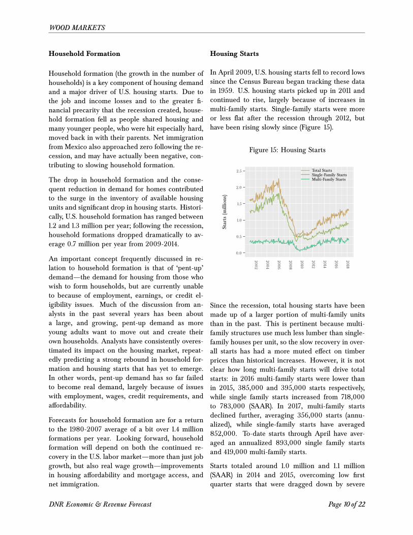
In April 2009, U.S. housing starts fell to record lowssince the Census Bureau began tracking these datain 1959. U.S. housing starts picked up in 2011 andcontinued to rise, largely because of increases inmulti-family starts. Single-family starts were moreor less flat after the recession through 2012, buthave been rising slowly since (Figure 15).

Figure 15: Housing Starts

0.0

0.5

1.0

1.5

2.0

2.5

2002

2004

2006

2008

2010

2012

2014

2016

2018

Starts(m

illions)

Total StartsSingle-Family StartsMulti-Family Starts

Since the recession, total housing starts have beenmade up of a larger portion of multi-family unitsthan in the past. This is pertinent because multi-family structures use much less lumber than single-family houses per unit, so the slow recovery in over-all starts has had a more muted effect on timberprices than historical increases. However, it is notclear how long multi-family starts will drive totalstarts: in 2016 multi-family starts were lower thanin 2015, 385,000 and 395,000 starts respectively,while single family starts increased from 718,000to 783,000 (SAAR). In 2017, multi-family startsdeclined further, averaging 356,000 starts (annu-alized), while single-family starts have averaged852,000. To-date starts through April have aver-aged an annualized 893,000 single family startsand 419,000 multi-family starts.

Starts totaled around 1.0 million and 1.1 million(SAAR) in 2014 and 2015, overcoming low firstquarter starts that were dragged down by severe

DNR Economic & Revenue Forecast Page 10 of 22

WOOD MARKETS

weather in both years. Housing starts in 2016and 2017 totaled 1.2 million (SAAR). Continued im-provements in household formations will increasedemand and drive an increase in starts, though itis unclear how long it will take before formationsincrease. Additionally, a recovery in house pricesshould facilitate the ‘move-up’ market. An increasein the move-up market combined with low total in-ventories constraining the supply of existing hous-ing should start increasing prices and provide in-centives to build more houses; again, this is likelyto be constrained by how much people can afford,so wages and lending standards will play a signifi-cant role.

Builder confidence is no longer an impediment tohousing starts, as estimates of confidence are con-sistent with housing starts of over 1 million. How-ever, there are significant supply impediments, suchas the shortage of buildable lots and permit de-lays. Given the lead time necessary to build houses,these are likely to cause volatility in both prices andsupply.

Housing Prices

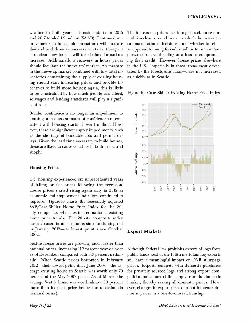
U.S. housing experienced six unprecedented yearsof falling or flat prices following the recession.House prices started rising again only in 2012 aseconomic and employment indicators continued toimprove. Figure 16 charts the seasonally adjustedS&P/Case-Shiller Home Price Index for the 20-city composite, which estimates national existinghome price trends. The 20-city composite indexhas increased in most months since bottoming outin January 2012—its lowest point since October2002.

Seattle house prices are growing much faster thannational prices, increasing 11.7 percent year-on-yearas of December, compared with 6.3 percent nation-ally. When Seattle prices bottomed in February2012—their lowest point since June 2004—the av-erage existing house in Seattle was worth only 70percent of the May 2007 peak. As of March, theaverage Seattle home was worth almost 30 percentmore than its peak price before the recession (innominal terms).

The increase in prices has brought back more nor-mal foreclosure conditions in which homeownerscan make rational decisions about whether to sell—as opposed to being forced to sell or to remain ‘un-derwater’ to avoid selling at a loss or compromis-ing their credit. However, house prices elsewherein the U.S.—especially in those areas most devas-tated by the foreclosure crisis—have not increasedas quickly as in Seattle.

Figure 16: Case-Shiller Existing Home Price Index

100

125

150

175

200

225

250

-30%

-20%

-10%

0%

10%

20%

30%

2001

2003

2005

2007

2009

2011

2013

2015

2017

2019

Hom

ePriceIndex

Ann

ual%

chan

ge

NationwideSeattle

Export Markets

Although Federal law prohibits export of logs frompublic lands west of the 108th meridian, log exportsstill have a meaningful impact on DNR stumpageprices. Exports compete with domestic purchasesfor privately sourced logs and strong export com-petition pulls more of the supply from the domesticmarket, thereby raising all domestic prices. How-ever, changes in export prices do not influence do-mestic prices in a one-to-one relationship.

Page 11 of 22 DNR Economic & Revenue Forecast

WOOD MARKETS

Figure 17: Log Export Prices

$0

$100

$200

$300

$400

$500

$600

$700

$800

$900

2005

2007

2009

2011

2013

2015

2017

$/mbf

(nom

inal)

Export PriceFEA Domestic PriceMill Survey Domestic Price

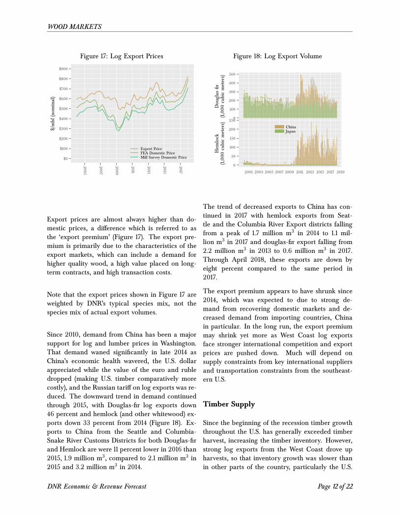
Export prices are almost always higher than do-mestic prices, a difference which is referred to asthe ‘export premium’ (Figure 17). The export pre-mium is primarily due to the characteristics of theexport markets, which can include a demand forhigher quality wood, a high value placed on long-term contracts, and high transaction costs.

Note that the export prices shown in Figure 17 areweighted by DNR’s typical species mix, not thespecies mix of actual export volumes.

Since 2010, demand from China has been a majorsupport for log and lumber prices in Washington.That demand waned significantly in late 2014 asChina’s economic health wavered, the U.S. dollarappreciated while the value of the euro and rubledropped (making U.S. timber comparatively morecostly), and the Russian tariff on log exports was re-duced. The downward trend in demand continuedthrough 2015, with Douglas-fir log exports down46 percent and hemlock (and other whitewood) ex-ports down 33 percent from 2014 (Figure 18). Ex-ports to China from the Seattle and Columbia-Snake River Customs Districts for both Douglas-firand Hemlock are were 11 percent lower in 2016 than2015, 1.9 million m3, compared to 2.1 million m3 in2015 and 3.2 million m3 in 2014.

Figure 18: Log Export Volume

0

100

200

300

400

500

0

50

100

150

200

250

2001 2003 2005 2007 2009 2011 2013 2015 2017 2019

Dou

glas-fir

(1,000

cubicmeters)

Hem

lock

(1,000

cubicmeters)

ChinaJapan

The trend of decreased exports to China has con-tinued in 2017 with hemlock exports from Seat-tle and the Columbia River Export districts fallingfrom a peak of 1.7 million m3 in 2014 to 1.1 mil-lion m3 in 2017 and douglas-fir export falling from2.2 million m3 in 2013 to 0.6 million m3 in 2017.Through April 2018, these exports are down byeight percent compared to the same period in2017.

The export premium appears to have shrunk since2014, which was expected to due to strong de-mand from recovering domestic markets and de-creased demand from importing countries, Chinain particular. In the long run, the export premiummay shrink yet more as West Coast log exportsface stronger international competition and exportprices are pushed down. Much will depend onsupply constraints from key international suppliersand transportation constraints from the southeast-ern U.S.

Timber Supply

Since the beginning of the recession timber growththroughout the U.S. has generally exceeded timberharvest, increasing the timber inventory. However,strong log exports from the West Coast drove upharvests, so that inventory growth was slower thanin other parts of the country, particularly the U.S.

DNR Economic & Revenue Forecast Page 12 of 22

WOOD MARKETS

South. Harvests have rebounded strongly enoughthat at some point in 2017, timber harvest beganto exceed growth, so the standing timber inventoryis beginning to fall. Drawing down the standingtimber inventory will constrain the region’s abilityto expand outputs—although harvests are expectedto continue to increase for several years, they willnot reach the levels of the mid-2000s, nor will theincreased harvest push prices down.

Since the late 1990s British Columbian forests havebeen devastated by the mountain timber beetle,which affected about a third of the province’s timberresources. Typically, timber killed by beetles mustbe harvested within 4 to 10 years so in 2007 thegovernment increased the allowable harvest to en-sure that the dead timber was not wasted, which in-creased British Columbia’s harvestable timber sup-ply. These elevated timber supplies are already de-clining. It’s expected that most of the beetle killwill be unviable by late 2017 and there will be noharvestable beetle kill after 2020. The supply fromCanada will be further diminished by Quebec’s al-lowable annual cut being reduced by Bill 57, whichwas implemented in April 2013, and may be ad-ditionally reduced by the ‘North for All’ plan (for-merly Plan Nord).

Price Outlook

Lumber Prices

As shown in Figure 11, lumber prices dropped pre-cipitously from mid-2014 to mid-2015, before lev-eling off. FEA’s coast lumber price peaked at$402/mbf in May 2014, but fell throughout the restof the year to average $376/mbf. This was largelydue to a bitterly cold winter across much of theU.S. which weakened domestic demand, ample lo-cal timber and lumber inventories, and the drop inexport demand from China. Prices in 2015 contin-ued their general downward trend and ended theyear averaging $317/mbf. Prices increased in 2016to average $341/mbf and increased sharply in 2017to average $425/mbf.

Prices early in 2017 were expected to spike withan anticipated imposition of countervailing and an-tidumping duties on Canadian lumber, which theUS Department of Commerce initiated in April.The additional duties had been expected sincethe end of the Softwood Lumber Agreement (SLA)in October 2015, which governed the quantity ofCanadian lumber imports allowed and duty levelsallowed based on lumber prices. Due to constraintsin the SLA, the U.S. was prevented from bringingany trade action against Canada until 12 October,2016. A petition was filed with the Department ofCommerce and the International Trade Commis-sion in November 2016.

Lumber prices were expected to spike prior to thenew duties, as lumber buyers increased orders toavoid the new taxes, but also increase after the du-ties were in place because they constrained supply.For the rest of 2017, lumber prices were expectedto be somewhat weaker as buyers drew down on in-ventory in anticipation of the slower building sea-son and a ’gap’ in the countervailing duties3. Thisprice weakness did not happened. Instead, pricesrose strongly through 2017 from $351/mbf in Jan-uary to $490/mbf in December.

Prices are expected to continue to increase throughthe second quarter of 2018, before falling back atthe end of the third quarter. Prices are expected todrop then due to the combination of the end of thebuilding season and increased supply from addi-tional capacity being put online. In outlying yearsprices are expected to remain higher than the 2017average, but will not reach the peaks of 2018.

Log Prices

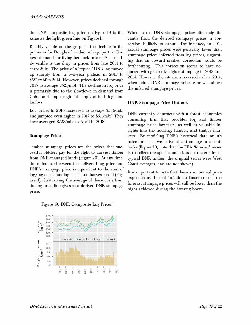
Figure 19 presents prices for Douglas-fir, hemlock,and DNR’s composite log. The latter is calcu-lated from prices for logs delivered to regionalmills, weighted by the average geographic location,species, and grade composition of timber typicallysold by DNR. In other words, it is the price a millwould pay for delivery of the typical log harvestedfrom DNR-managed lands. The dark green line for

3Apparently countervailing duties can only be collected for four months, but the International Trade Commission tookseveral months to make a final determination, meaning that there was a time gap when countervailing duties were not collected.

Page 13 of 22 DNR Economic & Revenue Forecast

WOOD MARKETS

the DNR composite log price on Figure 19 is thesame as the light green line on Figure 11.

Readily visible on the graph is the decline in thepremium for Douglas-fir—due in large part to Chi-nese demand fortifying hemlock prices. Also read-ily visible is the drop in prices from late 2014 toearly 2016. The price of a ‘typical’ DNR log movedup sharply from a two-year plateau in 2013 to$591/mbf in 2014. However, prices declined through2015 to average $521/mbf. The decline in log priceis primarily due to the slowdown in demand fromChina and ample regional supply of both logs andlumber.

Log prices in 2016 increased to average $536/mbfand jumpted even higher in 2017 to $611/mbf. Theyhave averaged $723/mbf to April in 2018.

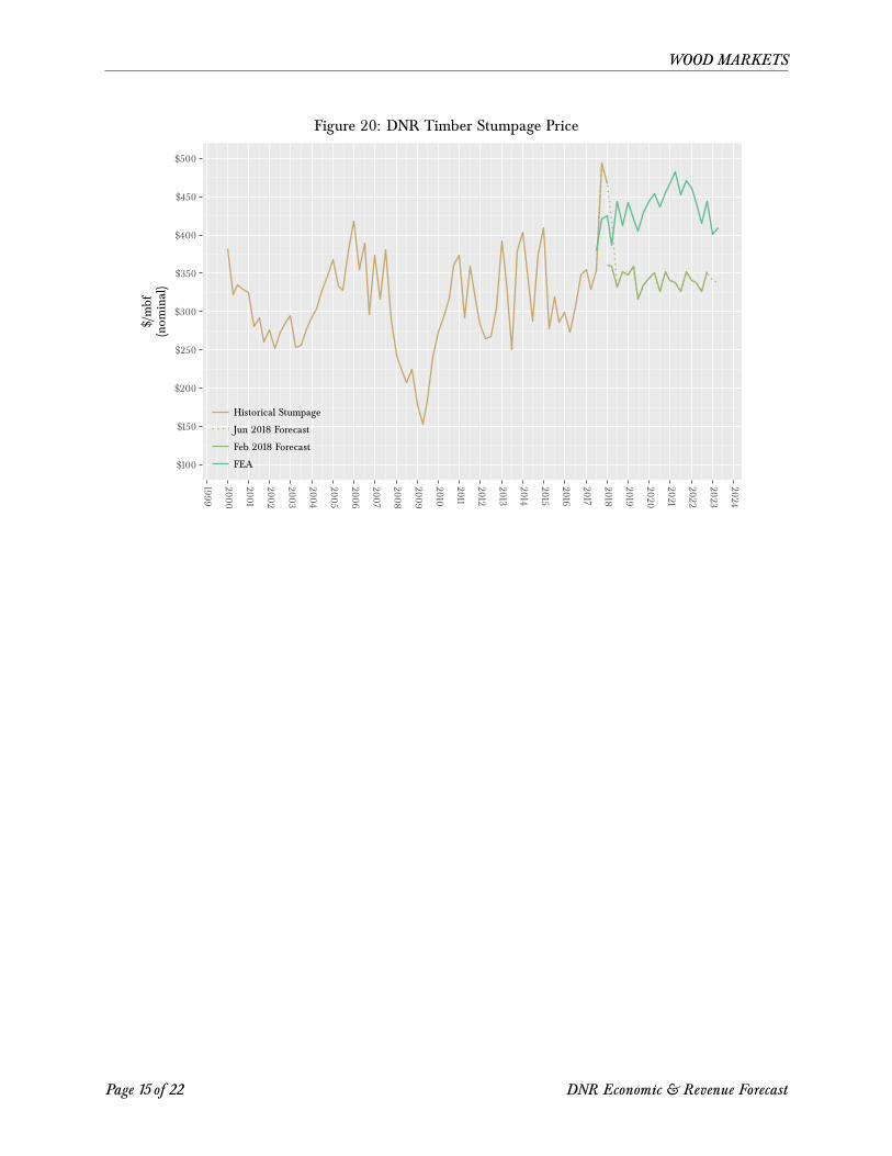
Stumpage Prices

Timber stumpage prices are the prices that suc-cessful bidders pay for the right to harvest timberfrom DNR-managed lands (Figure 20). At any time,the difference between the delivered log price andDNR’s stumpage price is equivalent to the sum oflogging costs, hauling costs, and harvest profit (Fig-ure 11). Subtracting the average of these costs fromthe log price line gives us a derived DNR stumpageprice.

Figure 19: DNR Composite Log Prices

$100$200$300$400$500$600$700

$0

$50

$100

$150

$200

$250

2001

2003

2005

2007

2009

2011

2013

2015

2017

2019

Log

Prices

$/mbf

Dou

glas-firPrem

ium

$/mbf

Douglas-fir Composite DNR Log Hemlock

When actual DNR stumpage prices differ signifi-cantly from the derived stumpage prices, a cor-rection is likely to occur. For instance, in 2012actual stumpage prices were generally lower thanstumpage prices inferred from log prices, suggest-ing that an upward market ‘correction’ would beforthcoming. This correction seems to have oc-curred with generally higher stumpage in 2013 and2014. However, the situation reversed in late 2014,when actual DNR stumpage prices were well abovethe inferred stumpage prices.

DNR Stumpage Price Outlook

DNR currently contracts with a forest economicsconsulting firm that provides log and timberstumpage price forecasts, as well as valuable in-sights into the housing, lumber, and timber mar-kets. By modeling DNR’s historical data on it’sprice forecasts, we arrive at a stumpage price out-looks (Figure 20, note that the FEA ‘forecast’ seriesis to reflect the species and class characteristics oftypical DNR timber; the original series were WestCoast averages, and are not shown).

It is important to note that these are nominal priceexpectations. In real (inflation adjusted) terms, theforecast stumpage prices will still be lower than thehighs achieved during the housing boom.

DNR Economic & Revenue Forecast Page 14 of 22

WOOD MARKETS

Figure 20: DNR Timber Stumpage Price

$100

$150

$200

$250

$300

$350

$400

$450

$500

1999

2000

2001

2002

2003

2004

2005

2006

2007

2008

2009

2010

2011

2012

2013

2014

2015

2016

2017

2018

2019

2020

2021

2022

2023

2024$/mbf

(nom

inal)

Historical Stumpage

Jun 2018 Forecast

Feb 2018 Forecast

FEA

Page 15 of 22 DNR Economic & Revenue Forecast

DNR REVENUE FORECAST

DNR Revenue Forecast

This Revenue Forecast includes revenue generatedfrom timber sales on trust uplands, leases on trustuplands, and leases on aquatic lands. It also fore-casts revenues to individual funds, including DNRmanagement funds, beneficiary current funds, andbeneficiary permanent funds. Caveats about theuncertainty of forecasting DNR-managed revenuesare summarized near the end of this section.

Timber Revenue

DNR sells timber through auctioned contracts thatvary in duration. For instance, contracts for DNRtimber sales sold in FY 2014 needed to be harvestedbetween three months and four and a half yearsfrom the date of sale, with an average (weighted byvolume) of about 25 months. The purchaser deter-mines the actual timing of harvest within the termsof the contract, which is likely based on perceptionsof market conditions. As a result, timber revenuesto beneficiaries and DNR management funds lagbehind sales.

For the purposes of this chapter, timber that is soldbut not yet harvested is referred to as ‘inventory’or ‘under contract’. Timber volume is added to theinventory when it is sold and placed under con-tract, and it is removed from the inventory whenthe timber is harvested.

Figure 21: Forecast Timber Sales Volume

400

500

600

700

800

2008

2010

2012

2014

2016

2018

2020

2022

mmbf,S

cribner

TS Volume FebTS Volume Jun

Timber Sales Volume

The sales volume forecast for FY 18 is reduced to495 mmbf due to some no-bid sales in recent auc-tions. Sales volume forecasts for all outlying yearsare unchanged (Figure 21).

FY 15 was the first year of the new sustainableharvest decade (FY 15 through FY 24) for westernWashington; however, new harvest targets for thissustainable harvest decade have not yet been de-termined or approved by the Board of Natural Re-sources. Without an updated sustainable harvestlimit, annual Westside sales volumes are forecast tobe 450 mmbf for future years. Together with pro-jected Eastside timber sales of 50 mmbf for eachof the next several years, we arrive at a projectedannual timber sales volume of about 500 mmbf forFYs 19-23.

Figure 22: Forecast Timber Removal Volume

0

100

200

300

400

500

600

700

800

900

2008

2009

2010

2011

2012

2013

2014

2015

2016

2017

2018

2019

2020

2021

2022

2023

mmbf,S

cribner

Removals to DateSales Under ContractSales in FY 18Sales in FY 19Sales in FY 20Sales in FY 21Sales in FY 22Sales in FY 23

Timber Removal Volume

For each Forecast, we survey timber sale purchasersto determine their planned harvest timing for thetimber volume they have under contract at the timeof the survey. This Forecast’s survey, conducted inthe first half of May, indicates that purchasers areplanning to harvest 112 mmbf of current inventory(686 mmbf) volume in the remaining two monthsof this fiscal year. This would mean an averageharvest volume of 55 mmbf per month, which is

DNR Economic & Revenue Forecast Page 16 of 22

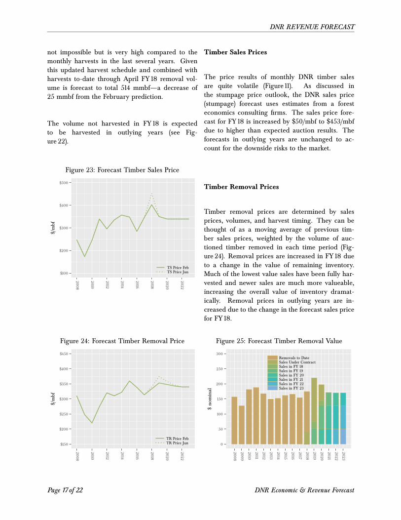
DNR REVENUE FORECAST

not impossible but is very high compared to themonthly harvests in the last several years. Giventhis updated harvest schedule and combined withharvests to-date through April FY 18 removal vol-ume is forecast to total 514 mmbf—a decrease of25 mmbf from the February prediction.

The volume not harvested in FY 18 is expectedto be harvested in outlying years (see Fig-ure 22).

Figure 23: Forecast Timber Sales Price

$100

$200

$300

$400

$500

2008

2010

2012

2014

2016

2018

2020

2022

$/mbf

TS Price FebTS Price Jun

Figure 24: Forecast Timber Removal Price

$150

$200

$250

$300

$350

$400

$450

2008

2010

2012

2014

2016

2018

2020

2022

$/mbf

TR Price FebTR Price Jun

Timber Sales Prices

The price results of monthly DNR timber salesare quite volatile (Figure 11). As discussed inthe stumpage price outlook, the DNR sales price(stumpage) forecast uses estimates from a foresteconomics consulting firms. The sales price fore-cast for FY 18 is increased by $50/mbf to $453/mbfdue to higher than expected auction results. Theforecasts in outlying years are unchanged to ac-count for the downside risks to the market.

Timber Removal Prices

Timber removal prices are determined by salesprices, volumes, and harvest timing. They can bethought of as a moving average of previous tim-ber sales prices, weighted by the volume of auc-tioned timber removed in each time period (Fig-ure 24). Removal prices are increased in FY 18 dueto a change in the value of remaining inventory.Much of the lowest value sales have been fully har-vested and newer sales are much more valueable,increasing the overall value of inventory dramat-ically. Removal prices in outlying years are in-creased due to the change in the forecast sales pricefor FY 18.

Figure 25: Forecast Timber Removal Value

0

50

100

150

200

250

300

2008

2009

2010

2011

2012

2013

2014

2015

2016

2017

2018

2019

2020

2021

2022

2023

$no

minal

Removals to DateSales Under ContractSales in FY 18Sales in FY 19Sales in FY 20Sales in FY 21Sales in FY 22Sales in FY 23

Page 17 of 22 DNR Economic & Revenue Forecast

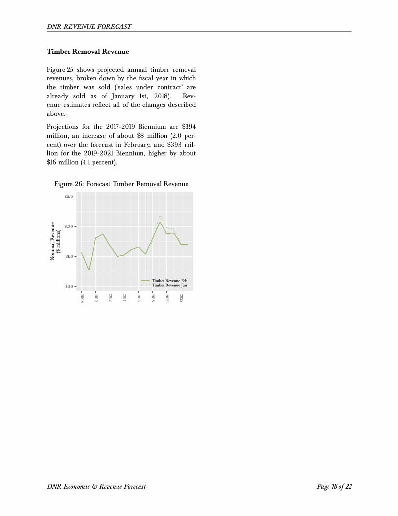
DNR REVENUE FORECAST

Timber Removal Revenue

Figure 25 shows projected annual timber removalrevenues, broken down by the fiscal year in whichthe timber was sold (‘sales under contract’ arealready sold as of January 1st, 2018). Rev-enue estimates reflect all of the changes describedabove.

Projections for the 2017-2019 Biennium are $394million, an increase of about $8 million (2.0 per-cent) over the forecast in February, and $393 mil-lion for the 2019-2021 Biennium, higher by about$16 million (4.1 percent).

Figure 26: Forecast Timber Removal Revenue

$100

$150

$200

$250

2008

2010

2012

2014

2016

2018

2020

2022

Nom

inal

Revenue

($millions)

Timber Revenue FebTimber Revenue Jun

DNR Economic & Revenue Forecast Page 18 of 22

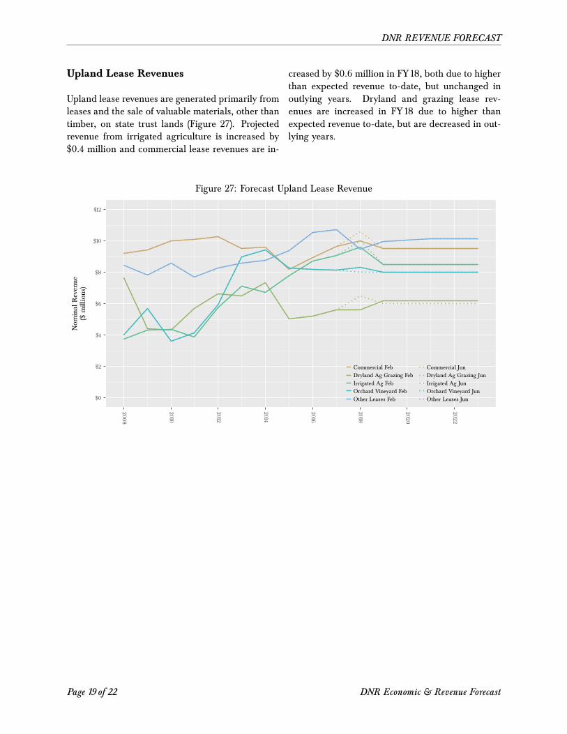
DNR REVENUE FORECAST

Upland Lease Revenues

Upland lease revenues are generated primarily fromleases and the sale of valuable materials, other thantimber, on state trust lands (Figure 27). Projectedrevenue from irrigated agriculture is increased by$0.4 million and commercial lease revenues are in-

creased by $0.6 million in FY 18, both due to higherthan expected revenue to-date, but unchanged inoutlying years. Dryland and grazing lease rev-enues are increased in FY 18 due to higher thanexpected revenue to-date, but are decreased in out-lying years.

Figure 27: Forecast Upland Lease Revenue

$0

$2

$4

$6

$8

$10

$12

2008

2010

2012

2014

2016

2018

2020

2022

Nom

inal

Revenue

($millions)

Commercial Feb Commercial JunDryland Ag Grazing Feb Dryland Ag Grazing JunIrrigated Ag Feb Irrigated Ag JunOrchard Vineyard Feb Orchard Vineyard JunOther Leases Feb Other Leases Jun

Page 19 of 22 DNR Economic & Revenue Forecast

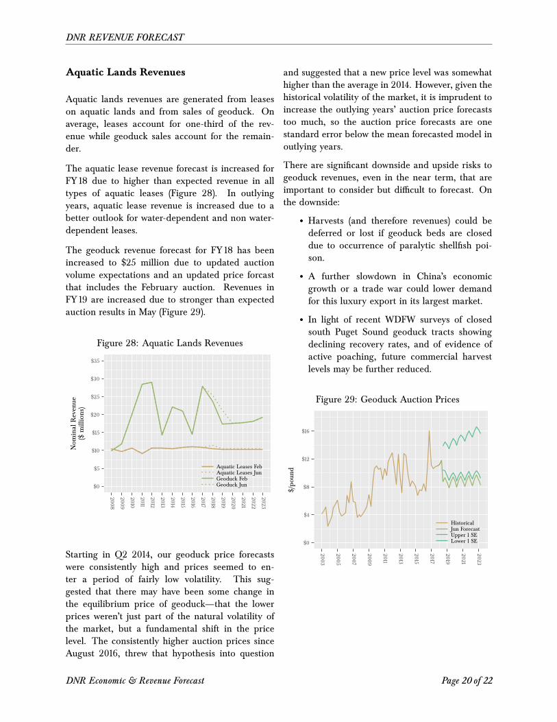
DNR REVENUE FORECAST

Aquatic Lands Revenues

Aquatic lands revenues are generated from leaseson aquatic lands and from sales of geoduck. Onaverage, leases account for one-third of the rev-enue while geoduck sales account for the remain-der.

The aquatic lease revenue forecast is increased forFY 18 due to higher than expected revenue in alltypes of aquatic leases (Figure 28). In outlyingyears, aquatic lease revenue is increased due to abetter outlook for water-dependent and non water-dependent leases.

The geoduck revenue forecast for FY 18 has beenincreased to $25 million due to updated auctionvolume expectations and an updated price forcastthat includes the February auction. Revenues inFY 19 are increased due to stronger than expectedauction results in May (Figure 29).

Figure 28: Aquatic Lands Revenues

$0

$5

$10

$15

$20

$25

$30

$35

2008

2009

2010

2011

2012

2013

2014

2015

2016

2017

2018

2019

2020

2021

2022

2023

Nom

inal

Revenue

($millions)

Aquatic Leases FebAquatic Leases JunGeoduck FebGeoduck Jun

Starting in Q2 2014, our geoduck price forecastswere consistently high and prices seemed to en-ter a period of fairly low volatility. This sug-gested that there may have been some change inthe equilibrium price of geoduck—that the lowerprices weren’t just part of the natural volatility ofthe market, but a fundamental shift in the pricelevel. The consistently higher auction prices sinceAugust 2016, threw that hypothesis into question

and suggested that a new price level was somewhathigher than the average in 2014. However, given thehistorical volatility of the market, it is imprudent toincrease the outlying years’ auction price forecaststoo much, so the auction price forecasts are onestandard error below the mean forecasted model inoutlying years.

There are significant downside and upside risks togeoduck revenues, even in the near term, that areimportant to consider but difficult to forecast. Onthe downside:

• Harvests (and therefore revenues) could bedeferred or lost if geoduck beds are closeddue to occurrence of paralytic shellfish poi-son.

• A further slowdown in China’s economicgrowth or a trade war could lower demandfor this luxury export in its largest market.

• In light of recent WDFW surveys of closedsouth Puget Sound geoduck tracts showingdeclining recovery rates, and of evidence ofactive poaching, future commercial harvestlevels may be further reduced.

Figure 29: Geoduck Auction Prices

$0

$4

$8

$12

$16

2003

2005

2007

2009

2011

2013

2015

2017

2019

2021

2023

$/po

und

HistoricalJun ForecastUpper 1 SELower 1 SE

DNR Economic & Revenue Forecast Page 20 of 22

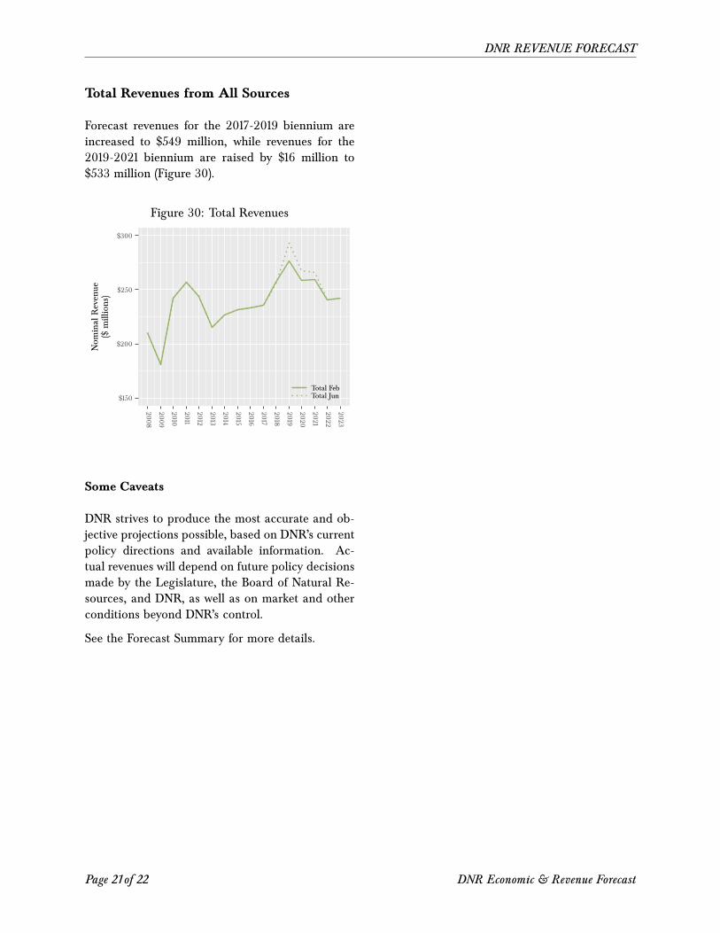
DNR REVENUE FORECAST

Total Revenues from All Sources

Forecast revenues for the 2017-2019 biennium areincreased to $549 million, while revenues for the2019-2021 biennium are raised by $16 million to$533 million (Figure 30).

Figure 30: Total Revenues

$150

$200

$250

$300

2008

2009

2010

2011

2012

2013

2014

2015

2016

2017

2018

2019

2020

2021

2022

2023

Nom

inal

Revenue

($millions)

Total FebTotal Jun

Some Caveats

DNR strives to produce the most accurate and ob-jective projections possible, based on DNR’s currentpolicy directions and available information. Ac-tual revenues will depend on future policy decisionsmade by the Legislature, the Board of Natural Re-sources, and DNR, as well as on market and otherconditions beyond DNR’s control.

See the Forecast Summary for more details.

Page 21 of 22 DNR Economic & Revenue Forecast

DNR REVENUE FORECAST

Distribution of Revenues

The distribution of timber revenues by trust arebased on:

• The volumes and values of timber in the in-ventory (sales sold but not yet harvested) bytrust;

• The volumes of timber in planned sales forFYs 17-18 by trust, and relative historical tim-ber prices by DNR region by trust; and

• The volumes of timber by trust for FYs 19-21 based on provisional output of the sus-tainable harvest model and relative historicaltimber prices by DNR region by trust.

Since a single timber sale can be worth more than$3 million, dropping, adding, or delaying even onesale can represent a significant shift in revenues toa specific trust fund.

Distributions of upland and aquatic lease revenuesby trust are assumed to be proportional to historicdistributions unless otherwise specified.

Management Fee Deduction. The underlyingstatutory management fee deductions to DNR asauthorized by the legislature are 25 percent or less,as determined by the Board of Natural Resources

(Board), for both the Resources Management CostAccount (RMCA) and the Forest Development Ac-count (FDA). In biennial budget bills, the Legisla-ture has authorized a deduction of up to 30 percentto RMCA since July 1, 2005. In 2015, they autho-rized a deduction up to 31 percent.

At its April 2011 meeting, the Board adopted a res-olution to reduce the RMCA deduction from 30 to27 percent and the FDA deduction from 25 to 23percent. At its July 2011 meeting, the Board de-cided to continue the deductions at 27 percent forRMCA (so long as this rate is authorized by the leg-islature) and at 23 percent for FDA. At its October2011 meeting, the Board approved a resolution toreduce the FDA deduction from 23 to 21 percent.The Board decided in July 2013 to raise the FDAdeduction to 25 percent and the RMCA deductionto 29 percent. In August 2015 the Board raised theRMCA deduction up to 31 percent for the 2015-2017biennium.

The Forecast uses the 31 percent deduction for the2017-2019 and 2019-2021 biennia. This assumesthat the Legislature will approve RMCA deductionsof up to 31 percent.

Given this background of official actions by the leg-islature and the Board, the management fee deduc-tions assumed in this Forecast are:

FY 2018 FY 2019 FY 2020 FY 2021 FY 2022 FY 2023FDA 25 25 25 25 25 25RMCA 31 31 31 31 31 31

DNR Economic & Revenue Forecast Page 22 of 22