Department of inorganic technology

Department of inorganic technology

LABORATORY WORK

Hydrocarbon separation on micro-porous membranes

Single gas permeance measurement

Milan Bernauer, Vlastimil Fíla, Vladimír Navara, Bohumil Bernauer and Petr �´astný

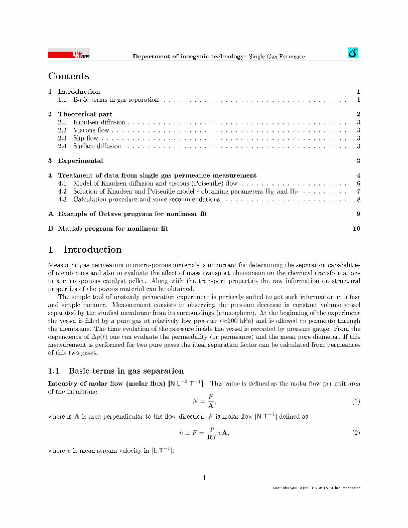
Department of inorganic technology: Single Gas Permeace

Contents

1 Introduction 11.1 Basic terms in gas separation . . . . . . . . . . . . . . . . . . . . . . . . . . . . . . . . . . . . 1

2 Theoretical part 22.1 Knudsen di�usion . . . . . . . . . . . . . . . . . . . . . . . . . . . . . . . . . . . . . . . . . . . 32.2 Viscous �ow . . . . . . . . . . . . . . . . . . . . . . . . . . . . . . . . . . . . . . . . . . . . . . 32.3 Slip �ow . . . . . . . . . . . . . . . . . . . . . . . . . . . . . . . . . . . . . . . . . . . . . . . . 32.4 Surface di�usion . . . . . . . . . . . . . . . . . . . . . . . . . . . . . . . . . . . . . . . . . . . 3

3 Experimental 3

4 Treatment of data from single gas permeance measurement 44.1 Model of Knudsen di�usion and viscous (Poiseuille) �ow . . . . . . . . . . . . . . . . . . . . . 64.2 Solution of Knudsen and Poiseuille model - obtaining parameters ΠK and ΠP . . . . . . . . . 74.3 Calculation procedure and some recommendations . . . . . . . . . . . . . . . . . . . . . . . . 8

A Example of Octave program for nonlinear �t 9

B Matlab program for nonlinear �t 10

1 Introduction

Measuring gas permeation in micro-porous materials is important for determining the separation capabilitiesof membranes and also to evaluate the e�ect of mass transport phenomena on the chemical transformationsin a micro-porous catalyst pellet. Along with the transport properties the raw information on structuralproperties of the porous material can be obtained.

The simple tool of unsteady permeation experiment is perfectly suited to get such information in a fastand simple manner. Measurement consists in observing the pressure decrease in constant volume vesselseparated by the studied membrane from its surroundings (atmosphere). At the beginning of the experimentthe vessel is �lled by a pure gas at relatively low pressure (≈500 kPa) and is allowed to permeate throughthe membrane. The time evolution of the pressure inside the vessel is recorded by pressure gauge. From thedependence of ∆p(t) one can evaluate the permeability (or permeance) and the mean pore diameter. If thismeasurement is performed for two pure gases the ideal separation factor can be calculated from permeancesof this two gases.

1.1 Basic terms in gas separation

Intensity of molar �ow (molar �ux) [N L−2 T−1] This value is de�ned as the molar �ow per unit areaof the membrane

N =F

A, (1)

where is A is area perpendicular to the �ow direction, F is molar �ow [N T−1] de�ned as

n ≡ F =p

RTvA, (2)

where v is mean stream velocity in [L T−1].

Last change: April 17, 2013 Milan Bernauer

1



Permeance [N M−1 T L−1] This value is de�ned as the ratio of the intensity of the molar �ow and thepressure di�erence on both side of the membrane

Π =N

∆p(3)

In conventional units the permeance is usually expressed in mol m−2 s−1 Pa−1.

Permeability [N M−1 T L−2] is a value of permeance related to the thickness of the membrane

β =Π

δ(4)

Ideal separation factor is a dimensionless value expressing the ratio of permeances (or permeabilities)of pure gases

Si,j =Πi

Πj=βiβj

(5)

2 Theoretical part

Permeation of gases through micro-porous solid is a complex phenomena including interactions between thepore wall and di�using molecules as well as interactions between di�using molecules themselves. Mechanismsgoverning the transport of gases in micro-porous media depends of physical properties of the material,experimental conditions and of course on permeating gas.

The micro-porous material can be characterized by the mean pore radius r, porosity ε and tortiuosity τ .The ratio of ε/τ is often expressed as ψ.

Experimental conditions in�uencing the permeation process are mainly temperature and pressure, whichdetermine the mean free path of the molecule λ

λ =RT

πNAdmp√

2, (6)

100200

300400

500

p/kPa

300400

500600

T/K

0

100

200

300

400

500

Kn

Figure 1: Knudsen number in ZSM-5 zeolite (2r =dp = 5.5 · 10−10m) as as function of p and T for N

2

(dm = 3 · 10−10 m).

where dm diameter of permeating molecule and NA

is Avogadro constant. The ratio

Kn =λ

2r, (7)

is called Knudsen number and its value give us theinformation about the nature of the mass transportmechanism inside the porous structure. Dependenceof Knudsen number on pressure and temperaturefor N

2in ZSM-5 zeolite is shown in �gure 1. For

numbers Kn > 1 the Knudsen di�usion is consid-ered to be the dominant contribution to the total�ow. For Kn < 1 the combination of viscous andslip �ow are dominantly responsible for the di�usionprocess. The surface di�usion occurs along all pre-viously transport mechanisms and has to be takeninto account at low temperatures for polar gases.

As evident from above paragraph total �ow of the permeating gas is a linear combination of di�erenttypes of di�usion processes.


2



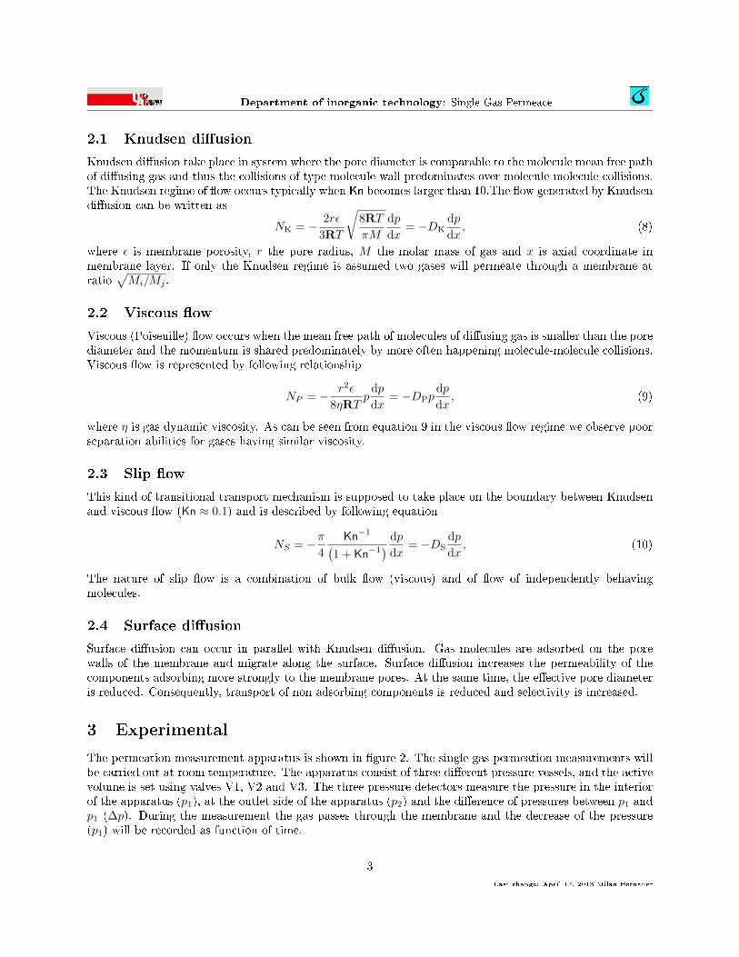
2.1 Knudsen di�usion

Knudsen di�usion take place in system where the pore diameter is comparable to the molecule mean free pathof di�using gas and thus the collisions of type molecule-wall predominates over molecule-molecule collisions.The Knudsen regime of �ow occurs typically when Kn becomes larger than 10.The �ow generated by Knudsendi�usion can be written as

NK = − 2rε

3RT

√8RT

πM

dp

dx= −DK

dp

dx, (8)

where ε is membrane porosity, r the pore radius, M the molar mass of gas and x is axial coordinate inmembrane layer. If only the Knudsen regime is assumed two gases will permeate through a membrane atratio

√Mi/Mj .

2.2 Viscous �ow

Viscous (Poiseuille) �ow occurs when the mean free path of molecules of di�using gas is smaller than the porediameter and the momentum is shared predominately by more often happening molecule-molecule collisions.Viscous �ow is represented by following relationship

NP = − r2ε

8ηRTp

dp

dx= −DPp

dp

dx, (9)

where η is gas dynamic viscosity. As can be seen from equation 9 in the viscous �ow regime we observe poorseparation abilities for gases having similar viscosity.

2.3 Slip �ow

This kind of transitional transport mechanism is supposed to take place on the boundary between Knudsenand viscous �ow (Kn ≈ 0.1) and is described by following equation

NS = −π4

Kn−1(1 + Kn−1

) dp

dx= −DS

dp

dx, (10)

The nature of slip �ow is a combination of bulk �ow (viscous) and of �ow of independently behavingmolecules.

2.4 Surface di�usion

Surface di�usion can occur in parallel with Knudsen di�usion. Gas molecules are adsorbed on the porewalls of the membrane and migrate along the surface. Surface di�usion increases the permeability of thecomponents adsorbing more strongly to the membrane pores. At the same time, the e�ective pore diameteris reduced. Consequently, transport of non adsorbing components is reduced and selectivity is increased.

3 Experimental

The permeation measurement apparatus is shown in �gure 2. The single gas permeation measurements willbe carried out at room temperature. The apparatus consist of three di�erent pressure vessels, and the activevolume is set using valves V1, V2 and V3. The three pressure detectors measure the pressure in the interiorof the apparatus (p1), at the outlet side of the apparatus (p2) and the di�erence of pressures between p1 andp1 (∆p). During the measurement the gas passes through the membrane and the decrease of the pressure(p1) will be recorded as function of time.


3



∆pp2 p1

v1 v2 v3

v6

v5v4

v7 v8

Figure 2: Experimental apparatus for unsteady permeation experiments. Valves v1 to v3 are destined to setthe volume of the vessel, valve v8 serve for �lling up the apparatus by chosen gas and valve v7 is used toopen the interior volume to the atmosphere (through the membrane).

4 Treatment of data from single gas permeance measurement

In our calculations we will consider only Knudsen di�usion and viscous �ow to participate to the total �owof the permeating gas.

As mentioned above, permeance of gas is de�ned as ratio of intensity of molar �ow N and the pressuregradient ∆p over the membrane

Π =N

∆p, (11)

where ∆p = p1(t) − p2, p1(t) is in our case pressure inside the vessel and p2 is atmospheric pressure. Infollowing text we omit (t) for simplicity. Material balance of permeation apparatus (�gure 3) is as follows

dn1

dt= −AN, (12)

where A is membrane cross section area and N is the intensity of molar �ow. For ideal gas we can write

dp1

dt= −ART

VN = QN. (13)

It is obvious thatdp1

dt=

d∆p

dt. (14)

Data obtained on the experimental apparatus are in the form of time dependence of pressure p1 (see �gure3). To obtain the value of N from equation 13 it is necessary to evaluate the derivative dp1/dt. This goalcould be achieved by several ways:


4



F2,iNi =AT

V

p 1

[ ] (t) (t)

(t)

][p(t )

t tx

x

p(t )xd

d tx

1

1

1

4p =p

Figure 3: A schematic picture of the permeation apparatus (left) and a typical output from permeancemeasurement (right).

Numerical di�erentiation Numerical derivation of obtained data can be done by using following rela-tionship

dp1

dt=

d∆p

dt≈p1,(t+∆t) − p1,(t)

∆t. (15)

This approach often fails because of the limited number precision of pressure gauge. This e�ect has an morepronounced impact specially at lower pressure di�erences or slower pressure decrease (see �gure 4). Thisinconvenience hampers the use of equation 15.

p

t

p(t )xd

d tx

tti

pi

p1

p2

t1 t2

< 0t1

p1

> 0t2

p2

Figure 4: A schematic picture of the numerical evaluation of dp/dt.


5



Polynomial representation of data The other way is to represent measured data by adequately chosenpolynomial function

p1(t) =

np∑i=1

aiti−1, (16)

where np is the number of parameters. The derivative dp1/dt is then calculated using following formula

dp1

dt=

d∆p

dt=

np∑i=1

(i− 1)aiti−2. (17)

The advantage of this approach is its simplicity and fast application. The disadvantage is the fact, thatby using an empirical formula (equation 16) we introduce uncertainty1 and by deriving this �uncertain�approximation (equation 17) we enhance this error by order of magnitude.

Using a representative ("real") model The most e�ort end time consuming approach is also the best.We derive a model, which represent the gas transport mechanism in porous media and derived relationship∆p = f(t) will be used to represent measured data. This approach is described in following section.

4.1 Model of Knudsen di�usion and viscous (Poiseuille) �ow

By solving di�erential equation 8 for membrane of thickness δ we obtain

NK = −DK

δ(p2 − p1) = ΠK∆p, (18)

where the parameter ΠK = DK/δ. We keep in mind that we choose in the �rst paragraph ∆p = p1 − p2 andthus the minus sign in equation 18 disappear.

By integration of equation 9 over a membrane of thickness δ we obtain

NP = −DP

2δ(p2

2 − p21) =

ΠP

2(p2

1 − p22) (19)

where the last therm (p21 − p2

2) can be transformed as follows

NP =Πp

2(p1 − p2)(p1 + p2) = ΠP(

∆p2

2+ p2∆p) (20)

This two above mentioned mechanism of gas transport occurs in parallel and their contribution to thetotal �ow can be represented by their linear combination

N = NP +NK = ΠP(∆p2

2+ p2∆p) + ΠK∆p (21)

From equation 11 and equation 23 one can evaluate the permeance as function of the pressure di�erence

Π =1

2ΠP∆p+ ΠPp2 + ΠK (22)

1In other words we are not describing the exact nature of the di�usion process.


6



4.2 Solution of Knudsen and Poiseuille model - obtaining parameters ΠK andΠP

By substituting N in equation 13 by equation 21 we obtain

d∆p

dt= Q(

1

2ΠP∆p2 + (ΠPp2 + ΠK)∆p.) (23)

The solution of di�erential equation 23 is as follows (after subsequent evaluation of ∆p)

∆p = 2Kexp{KQt+ C1}

ΠP −ΠP exp{KQt+ C1}, (24)

where K = ΠPp2 + ΠK. The adjustable parameters are K, ΠP a C1. Their estimation can be obtained fromnonlinear regression procedure of experimental data, i.e. by nonlinear �t of ∆p(t) data by equation 24. Thistask is quite complicated because of strong correlation between unknowns parameters. To avoid unsuccessfulconvergence of nonlinear estimation procedure, we have to rearrange the equation 24 in following way

∆p = Lexp{KQt+ C1}

1− exp{KQt+ C1}, (25)

whereL = 2(p2 + ΠK/ΠP) (26)

For nonlinear regression it is primordial to choose "good" initial estimates of �tted parameters. For parameterL we can calculate the ratio ΠK/ΠP in equation 26 from 8 and 9 as

ΠK/ΠP =32

3

η

r

√2RT

πM. (27)

For temperature around 298.15 K this ratio is approximately equal to

ΠK/ΠP(298 K) = 635.6η

r√M

(28)

This equation provide the initial estimate of parameter L (through equation 26).The initial estimate of C1 parameter is given by

C1 = ln

(∆p0

∆p0 + L

), (29)

where ∆p0 is the initial pressure di�erence.Values of ΠK a ΠP are then computed from parameters obtained from nonlinear regression by following

relationships

ΠK = K

(1− 2p2

L

)(30)

ΠP = 2K

L(31)

The �ux is then evaluated from equation 21 using parameters 30 and 31

N =K

L∆p2 +K∆p. (32)

The permeance as function of pressure di�erence is then calculated from equation 22

Π =K

L∆p+K. (33)


7Last change: April 17, 2013 Milan Bernauer


4.3 Calculation procedure and some recommendations

1. Fitting of measured data

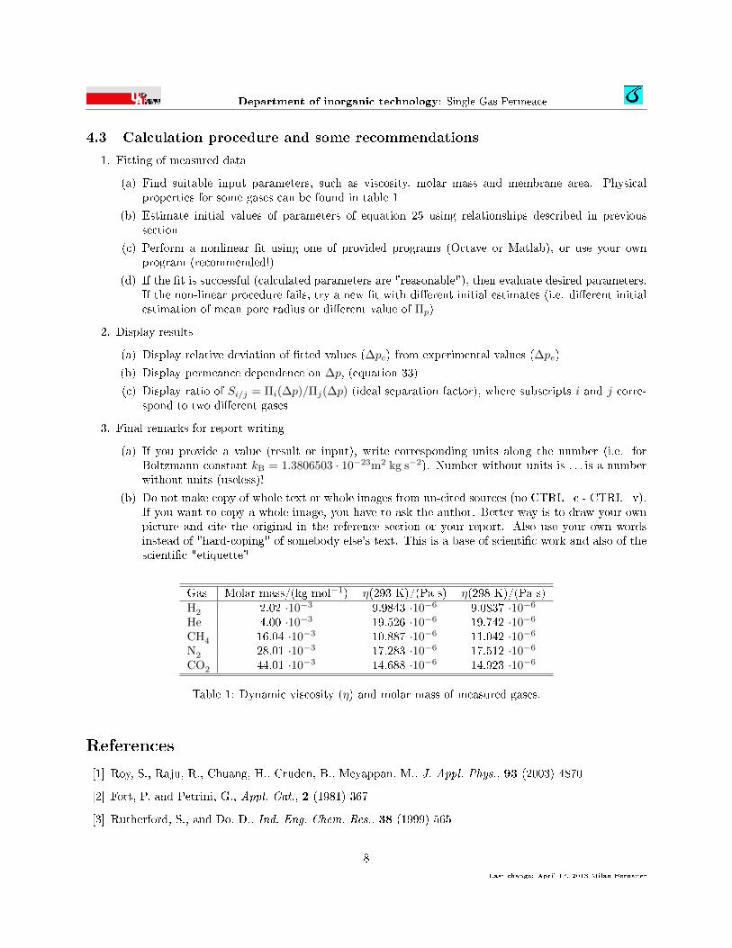
(a) Find suitable input parameters, such as viscosity, molar mass and membrane area. Physicalproperties for some gases can be found in table 1

(b) Estimate initial values of parameters of equation 25 using relationships described in previoussection

(c) Perform a nonlinear �t using one of provided programs (Octave or Matlab), or use your ownprogram (recommended!)

(d) If the �t is successful (calculated parameters are "reasonable"), then evaluate desired parameters.If the non-linear procedure fails, try a new �t with di�erent initial estimates (i.e. di�erent initialestimation of mean pore radius or di�erent value of Πp)

2. Display results

(a) Display relative deviation of �tted values (∆pc) from experimental values (∆pe)

(b) Display permeance dependence on ∆p, (equation 33)

(c) Display ratio of Si/j = Πi(∆p)/Πj(∆p) (ideal separation factor), where subscripts i and j corre-spond to two di�erent gases

3. Final remarks for report writing

(a) If you provide a value (result or input), write corresponding units along the number (i.e. forBoltzmann constant kB = 1.3806503 · 10−23m2 kg s−2). Number without units is . . . is a numberwithout units (useless)!

(b) Do not make copy of whole text or whole images from un-cited sources (no CTRL+c - CTRL+v).If you want to copy a whole image, you have to ask the author. Better way is to draw your ownpicture and cite the original in the reference section or your report. Also use your own wordsinstead of "hard-coping" of somebody else's text. This is a base of scienti�c work and also of thescienti�c "etiquette"

Gas Molar mass/(kg mol−1) η(293 K)/(Pa s) η(298 K)/(Pa s)H2 2.02 ·10−3 9.9843 ·10−6 9.0837 ·10−6

He 4.00 ·10−3 19.526 ·10−6 19.742 ·10−6

CH4 16.04 ·10−3 10.887 ·10−6 11.042 ·10−6

N2 28.01 ·10−3 17.283 ·10−6 17.512 ·10−6

CO2 44.01 ·10−3 14.688 ·10−6 14.923 ·10−6

Table 1: Dynamic viscosity (η) and molar mass of measured gases.

References

[1] Roy, S., Raju, R., Chuang, H., Cruden, B., Meyappan, M., J. Appl. Phys., 93 (2003) 4870

[2] Fott, P. and Petrini, G., Appl. Cat., 2 (1981) 367

[3] Rutherford, S., and Do, D., Ind. Eng. Chem. Res., 38 (1999) 565


8



0.5346

0.5347

0.5348

0.5349

0.535

0.5351

0.5352

0.5353

0.5354

100 150 200 250 300 350 400 450 500

S (

i/j)

∆ p/kPa

Separation factor

S(i/j)

0.4

0.6

0.8

1

1.2

1.4

1.6

100 150 200 250 300 350 400 450 500

Π 1

05/(

mol-1

s-1

m-2

Pa

-1)

∆p/kPa

Permenance

HeH2

-0.015

-0.01

-0.005

0

0.005

0.01

0 200 400 600 800 1000 1200 1400

r d

t / s

Rel. deviation of fit

HeH2

0

200

400

600

800

1000

0 200 400 600 800 1000 1200 1400

p /

kP

a

t / s

Measured data

HeH2

Figure 5: Measured data (∆p(t)), relative deviation of �t (rd = (∆pc − ∆pe)/∆pe), permeance and idealseparation factor of CH4 and H2 as function of pressure di�erence on titanosilicate membrane.

A Example of Octave program for nonlinear �t

%% This program calculates the coefficients p() resulting from

%% non-linear regression fit of data (data.txt) by function F

T = 298.15; % Temperature [K]

R = 8.314; % Univeral gas constant [J/mol/K]

V = 0.544e-3; % Apparatus volume [m3]

A = 0.7274635e-4; % Membrane area (membrane type K) [m2]

eta= 11.042e-6; % Gas dymanic viscosity (CH4) [Pa.s]

Mw = 16e-3; % Molar mass (CH4) [kg/mol]

rp = 1e-7; % Mean pore radius estimate [m]

val= dlmread('data.txt'); % Read input data from file

y = val(:,2)*1e3-val(:,4)*1e3; % Independent variables

x = val(:,1); % Dependent variable

[npts,trash] = size(x); % Read n. of points [npts]

Q = -R*T*A/V; % Q constant


9



%% Intial estimates

p2 = sum(val(:,4))*1e3/npts; % Mean atmospheric pressure [Pa]

dp0= (val(1,2) - val(1,4))*1e3; % Initial pressure difference [Pa]

%% L

pin(1) = 2*p2 + 32*eta/(2*rp)*sqrt(2*R*T/(3.1415926*Mw));

%% K

pin(2) = pin(1)*1.0e-11;

%% C

pin(3) = log(dp0/(dp0+pin(1)));

%% --------

ndf = (npts - 3); % N. deg. of freedom

wt = ones(size(x)); % Weigths

niter = 100; % Max. num. of iteration for non-lin. fit

stol = 1e-9; % Tolerance (stop. criterion)

%

%% Function to fit

F = @(x,p)(p(1).*(exp(p(2).*Q.*x(:,1) + p(3))./( 1 - exp(p(2).*Q.*x(:,1) + p(3))) ));

%% This is the Octave fitting routine for explanation read:

%% http://octave.sourceforge.net/optim/function/leasqr.html

%% [f,p,cvg,iter,corp,covp,covr,stdresid,Z,r2]=

%% leasqr(x,y,pin,F,{stol,niter,wt,dp,dFdp,options})

dFdp = 'dfdp';

dp = [1e-6; 1.e-6; 1.e-6];

[f,p,kvg,iter,corp,covp,covr,stdresid,Z,r2] = leasqr(x, y, pin, F,stol,niter,wt,dp,dFdp);

%% RESULTS

fprintf('L = %12.4e\n', p(1));

fprintf('K = %12.4e\n', p(2));

fprintf('C = %12.4e\n', p(3));

fprintf('iter = %4i\n', iter);

fprintf('ndf = %4i\n', ndf);

fprintf('WSSR = %12.4e\n', sqrt(sum((f(:)-y(:)).^2)./ndf));

fprintf('PIk = %12.4e\n', p(2).*(1-2*p2./p(1)));

fprintf('PIp = %12.4e\n', p(2)/p(1));

fprintf('rp = %12.4e\n', (32/2)/(p(1)-2*p2)*eta*sqrt(2*R*T/3.1415926/Mw));

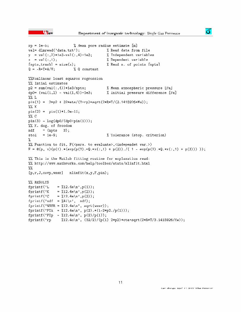
B Matlab program for nonlinear �t

%% This program calculates the coefficients p() resulting from

%% non-linear regression fit of data (data.txt) by function F

T = 298.15; % Temperature [K]

R = 8.314; % Univeral gas constant [J/mol/K]

V = 0.544e-3; % Apparatus volume [m3]

A = 0.7274635e-4; % Membrane area (membrane type K) [m2]

eta= 11.042e-6; % Gas dymanic viscosity (CH4) [Pa.s]

Mw = 16e-3; % Molar mass (CH4) [kg/mol]


10



rp = 1e-5; % Mean pore radius estimate [m]

val= dlmread('data.txt'); % Read data from file

y = val(:,2)*1e3-val(:,4)*1e3; % Independent variables

x = val(:,1); % Dependent variable

[npts,trash] = size(x); % Read n. of points [npts]

Q = -R*T*A/V; % Q constant

%%Nonlinear least squares regression

%% Intial estimates

p2 = sum(val(:,4))*1e3/npts; % Mean atmospheric pressure [Pa]

dp0= (val(1,2) - val(1,4))*1e3; % Initial pressure difference [Pa]

%% L

pin(1) = 2*p2 + 32*eta/(2*rp)*sqrt(2*R*T/(3.1415926*Mw));

%% K

pin(2) = pin(1)*1.0e-11;

%% C

pin(3) = log(dp0/(dp0+pin(1)));

%% N. deg. of freedom

ndf = (npts - 3);

stol = 1e-9; % Tolerance (stop. criterion)

%

%% Function to fit, F(<pars. to evaluate>,<independet var.>)

F = @(p, x)(p(1).*(exp(p(2).*Q.*x(:,1) + p(3))./( 1 - exp(p(2).*Q.*x(:,1) + p(3))) ));

%% This is the Matlab fitting routine for explanation read:

%% http://www.mathworks.com/help/toolbox/stats/nlinfit.html

%%

[p,r,J,covp,wssr] = nlinfit(x,y,F,pin);

%% RESULTS

fprintf('L = %12.4e\n',p(1));

fprintf('K = %12.4e\n',p(2));

fprintf('C = %12.4e\n',p(3));

fprintf('ndf = %4i\n', ndf);

fprintf('WSSR = %12.4e\n', sqrt(wssr));

fprintf('PIk = %12.4e\n', p(2).*(1-2*p2./p(1)));

fprintf('PIp = %12.4e\n', p(2)/p(1));

fprintf('rp = %12.4e\n', (32/2)/(p(1)-2*p2)*eta*sqrt(2*R*T/3.1415926/Mw));


11


Documents

Department of inorganic technology